Spatial Variability of Living Coccolithophore Distribu ... · Bering Sea water as result of an El...

505

Journal of Oceanography, Vol. 60, pp. 505 to 515, 2004

Keywords:⋅ Coccolithophores,⋅ vertical distribu-tion,⋅ western subarcticPacific,⋅ Bering Sea,⋅ calcite.

* Corresponding author. E-mail: [email protected]

† Present address: Aquaculture Department, Southeast Asian FisheriesDevelopment Center, Tigauan, Iloilo, Philippines.

Copyright © The Oceanographic Society of Japan.

Spatial Variability of Living Coccolithophore Distribu-tion in the Western Subarctic Pacific and Western BeringSea

HIROSHI HATTORI1*, MAKOTO KOIKE1, KENICHI TACHIKAWA1, HIROAKI SAITO2

and KAZUYA NAGASAWA3†

1Department of Marine Sciences and Technology, Hokkaido Tokai University, Minamisawa, Minami-ku, Sapporo 005-8601, Japan2Fisheries Oceanography, Tohoku National Fisheries Research Institute, Shinhamamachi, Shiogama 985-0001, Japan3National Research Institute of Far Seas Fisheries, Shimizu-Orido, Shimizu 424-8633, Japan

(Received 21 April 2003; in revised form 29 December 2003; accepted 5 January 2004)

Vertical distributions of coccolithophores were observed in the depth range 0–50 min the western subarctic Pacific and western Bering Sea in summer, 1997. Thirty-fivespecies of coccolithophores were collected. Overall, Emiliania huxleyi var. huxleyi wasthe most abundant taxon, accounting for 82.8% of all coccolithophores, although itwas less abundant in the western Bering Sea. Maximum abundance of this specieswas found in an area south of 41°N and east of 175°E (Transition Zone) reaching>10,000 cells L–1 in the water column. In addition to this species, Coccolithus pelagicusf. pelagicus, which accounted for 4.2% of the assemblage, was representative of thecoccolithophore standing crop in the western part of the subarctic Pacific. Coccolithuspelagicus f. hyalinus was relatively abundant in the Bering Sea, accounting for 2.6%of the assemblage. Coccolithophore standing crops in the top 50 m were high south of41°N (>241 × 106 cells m–2) and east of 170°E (542 × 106 cells m–2) where temperatureswere higher than 12°C and salinities were greater than 34.2. The lowest standing cropwas observed in the Bering Sea and Oyashio areas where temperatures were lowerthan 6–10°C and salinities were less than 33.0. From the coccolithophore volumes,the calcite stocks in the Transition, Subarctic, and the Bering Sea regions were esti-mated to be 73.0, 9.7, and 6.9 mg m–2, respectively, corresponding to calcite fluxes of3.6, 0.5, and 0.3 mg m–2d–1 using Stoke’s Law.

where they have an impact on not only biogeochemicalcycles but also food-web dynamics (Baduini et al., 2001;Olson and Strom, 2002). Due to their biogeochemical andecological significance, coccolithophores have been ex-tensively studied in the regions where these blooms fre-quently occur, e.g., the North Atlantic Ocean (Holliganet al., 1993b) and the Bering Sea (Stockwell et al., 2001).

In comparison with the many studies of the easternBering Sea and northern North Atlantic Ocean, studies inthe North Pacific, especially in the western subarctic Pa-cific, are quite limited. Okada and Honjo (1973) reportedthe spatial distribution and species composition ofcoccolithophores in the North Pacific Ocean. They founda high abundance (>105 cells L–1) of Emiliania huxleyi inthe eastern subarctic Pacific (north of 46°N, along155°W), but reported few data for the western subarcticPacific and the western Bering Sea. Sinking particles col-

1. IntroductionCoccolithophores are found in great abundance in

many marine ecosystems. Because of their high biomassand unique physiology, they are key agents of biologicalforcing of global climate (Westbroek et al., 1993). Pro-duction of calcium carbonate reduces seawater alkalin-ity, which decreases CO2 influx from air to the ocean(Balch et al., 1992; Paasche, 2002). Coccolithophoresemit dimethyl sulfide (DMS) that potentially enhancescloud albedo (e.g., Burkill et al., 2002). Coccolithophoresform “blooms” both in the coastal and oceanic waters,

506 H. Hattori et al.

lected by sediment traps showed large seasonal variabil-i ty in the production of E. huxleyi and othercoccolithophores in the central subarctic Pacific andBering Sea (Takahashi et al., 2000) and in the OkhotskSea (Broerse et al., 2000). In the western subarctic Pa-cific, CaCO3 fluxes are similar to those in the other re-gions of the subarctic Pacific and its adjacent seas buthave a smaller seasonal variability (Noriki and Tsunogai,1986; Honda et al., 2002). Seasonal changes in total al-kalinity suggest that the calcification rate was very lowin the western subarctic Pacific compared with the cen-tral and eastern subarctic Pacific (Wong et al., 2002),which, in turn, suggests a low production rate ofcoccolithophores in this region. Using satellite images,Takahashi et al. (1995) reported coccolithophore blooms(revealed by high reflectance waters) in the area between35°N and 50°N of the western North Pacific. Althoughthese studies indicate the occurrence of coccolithophoresin the western subarctic Pacific and western Bering Sea,we lack direct information of coccolithophore distribu-tion and species composition in these regions.

During September 1997, an extensivecoccolithophore bloom was first observed by satellite inthe southeastern Bering Sea (cf. Stockwell et al., 2001).The concentration of E. huxleyi in this bloom water byAugust/September was reported as 2.95 × 105 cells L–1

(Stockwell et al., 2001). This large-scale bloom in theBering Sea was considered to represent a warming ofBering Sea water as result of an El Niño event (cf. Minobe,2002). Minobe (2002) reported that the temperature in1997 was the warmest it had been over the preceding fewdecades. In the present study we examined the distribu-tion and species composition of coccolithophores in thewestern subarctic Pacific and western Bering Sea to com-pare them with the standing stocks in the eastern part andto estimate the flux of coccolithophores during summerin 1997, just a coincidence in an El Niño/Southern OceanOscillation year.

2. Material and MethodsWater samples were taken for coccolithophore counts

and chlorophyll a measurements during a cruise of the R/V Wakatake Maru conducted between 13 June and 23 July,1997 in the western part of the northern North Pacificand western Bering Sea. Samples were taken at 0, 10, 20,30, and 50 m water depths with Niskin bottles. Observa-tions were made along three transects: a 180° meridiantransect (Stns. 1–21), a 40°N latitude transect (Stns. T1–T26), and a Kuril Islands-Kamchatka transect (KI; Stns.T52–T77) (Fig. 1). Stn. T1 and Stn. T77 were in the samelocation, but observations were made on 13 June at Stn.T1 and on 23 July at Stn. 77. Temperature and salinitywere recorded from the surface to a depth of 100 m withan Alec P-1000 STD.

One liter of the seawater was fixed with 2% (v/v)buffered formalin (pH = 7.8) for coccolithophore counts.A portion of this water (70–100 mL) was filtered througha Nuclepore membrane filter (0.8 µm pore size) using aglass funnel (8 mm in diameter at the base). During fil-tering, the vacuum was kept at approximately 10–20 cmHg. The filter membrane was rinsed with distilled waterto remove all salt and immediately dried for several hoursin an oven at 40–60°C. To count and identify specimens,the whole area of the membrane (>50 mm2) was exam-ined with a scanning electron microscope (JOEL, JMS-840A) at a magnification of about 2,000×. Placolith (frag-ment of cell) was not counted in the cell number. Specieswere identified according to Winter and Siesser (1994).The abundances of coccolithophores at Stns. 18 and 19in the Bering Sea were shown as one station due to con-fusion of the sample water taken at a certain depth.

For chlorophyll a analysis, freshly collected seawaterwas filtered through a Whatman GF/F filter, which wasthen frozen at –50°C until analysis. Chlorophyll a con-centration was determined fluorometrically after extrac-tion by 90% acetone (Parsons et al., 1984).

3. Results and Discussion

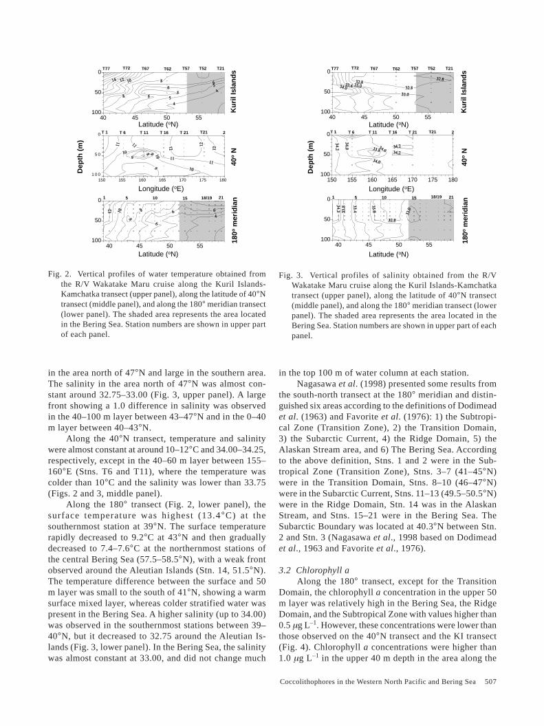
3.1 Temperature and salinityAlong the KI transect, the surface temperature in-

creased from 7–8°C at the northernmost stations locatedbetween 58.5–55.5°N to 21.7°C at the southernmost sta-tion at 40°N (Fig. 2, upper panel). The temperature dif-ference between the surface and the 100 m layer was small

Fig. 1. Sampling locations covered during the R/V WakatakeMaru cruise between 13 June and 23 July, 1997. Along the180° meridian transect, the survey region was divided intofive water masses in the North Pacific by Nagasawa et al.(1998): subtropical North Pacific = Transition Zone (ST:TZ), Transition Domain (TD), Subarctic Current (SC), RidgeDomain (RD), and Alaskan Stream (AS). BS represents theBering Sea.

Coccolithophores in the Western North Pacific and Bering Sea 507

in the area north of 47°N and large in the southern area.The salinity in the area north of 47°N was almost con-stant around 32.75–33.00 (Fig. 3, upper panel). A largefront showing a 1.0 difference in salinity was observedin the 40–100 m layer between 43–47°N and in the 0–40m layer between 40–43°N.

Along the 40°N transect, temperature and salinitywere almost constant at around 10–12°C and 34.00–34.25,respectively, except in the 40–60 m layer between 155–160°E (Stns. T6 and T11), where the temperature wascolder than 10°C and the salinity was lower than 33.75(Figs. 2 and 3, middle panel).

Along the 180° transect (Fig. 2, lower panel), thesurface temperature was highest (13.4°C) at thesouthernmost station at 39°N. The surface temperaturerapidly decreased to 9.2°C at 43°N and then graduallydecreased to 7.4–7.6°C at the northernmost stations ofthe central Bering Sea (57.5–58.5°N), with a weak frontobserved around the Aleutian Islands (Stn. 14, 51.5°N).The temperature difference between the surface and 50m layer was small to the south of 41°N, showing a warmsurface mixed layer, whereas colder stratified water waspresent in the Bering Sea. A higher salinity (up to 34.00)was observed in the southernmost stations between 39–40°N, but it decreased to 32.75 around the Aleutian Is-lands (Fig. 3, lower panel). In the Bering Sea, the salinitywas almost constant at 33.00, and did not change much

in the top 100 m of water column at each station.Nagasawa et al. (1998) presented some results from

the south-north transect at the 180° meridian and distin-guished six areas according to the definitions of Dodimeadet al. (1963) and Favorite et al. (1976): 1) the Subtropi-cal Zone (Transition Zone), 2) the Transition Domain,3) the Subarctic Current, 4) the Ridge Domain, 5) theAlaskan Stream area, and 6) The Bering Sea. Accordingto the above definition, Stns. 1 and 2 were in the Sub-tropical Zone (Transition Zone), Stns. 3–7 (41–45°N)were in the Transition Domain, Stns. 8–10 (46–47°N)were in the Subarctic Current, Stns. 11–13 (49.5–50.5°N)were in the Ridge Domain, Stn. 14 was in the AlaskanStream, and Stns. 15–21 were in the Bering Sea. TheSubarctic Boundary was located at 40.3°N between Stn.2 and Stn. 3 (Nagasawa et al., 1998 based on Dodimeadet al., 1963 and Favorite et al., 1976).

3.2 Chlorophyll aAlong the 180° transect, except for the Transition

Domain, the chlorophyll a concentration in the upper 50m layer was relatively high in the Bering Sea, the RidgeDomain, and the Subtropical Zone with values higher than0.5 µg L–1. However, these concentrations were lower thanthose observed on the 40°N transect and the KI transect(Fig. 4). Chlorophyll a concentrations were higher than1.0 µg L–1 in the upper 40 m depth in the area along the

40 45 50 55100

50

0

150 155 160 165 170 175 1801 0 0

5 0

0

40 45 50 55100

50

0

Dep

th (

m)

Latitude (oN)

180o

mer

idia

n

Longitude (oE)

40o N

Latitude (oN)

Ku

ril I

slan

dsT77 T72 T67 T62 T57 T52 T21

T 1 T 6 T 11 T 16 T 21 T21 2

1 5 10 15 2118/19

Dep

th (

m)

Latitude (oN)

180o

mer

idia

n

Longitude (oE)

40o N

Latitude (oN)

Ku

ril I

slan

ds

40 45 50 55100

50

0

150 155 160 165 170 175 180100

50

0

40 45 50 55100

50

0

T77 T72 T67 T62 T57 T52 T21

T 1 T 6 T 11 T 16 T 21 T21 2

1 5 10 15 2118/19

Fig. 2. Vertical profiles of water temperature obtained fromthe R/V Wakatake Maru cruise along the Kuril Islands-Kamchatka transect (upper panel), along the latitude of 40°Ntransect (middle panel), and along the 180° meridian transect(lower panel). The shaded area represents the area locatedin the Bering Sea. Station numbers are shown in upper partof each panel.

Fig. 3. Vertical profiles of salinity obtained from the R/VWakatake Maru cruise along the Kuril Islands-Kamchatkatransect (upper panel), along the latitude of 40°N transect(middle panel), and along the 180° meridian transect (lowerpanel). The shaded area represents the area located in theBering Sea. Station numbers are shown in upper part of eachpanel.


40°N transect (except at Stn. T21 at 170°E) and the areaalong the KI transect between 44 and 52°N with valuesreaching 2.5 µg L–1 at 47°N.

Although the chlorophyll a concentration in thepresent study area varies interannually (Shiomoto et al.,1999), the concentrations observed in the Transition Do-main (<0.5 µg L–1) in summer were always lower thanthose in other areas (>0.5 µg L–1) as was observed byother studies (Banse and English, 1999; Shiomoto et al.,1999; Hayashi et al., 2001). Shiomoto et al. (1999) sug-gested that this low concentration in the Transition Do-main was due to heavy grazing by zooplankton. We ob-served higher concentrations (0.5 to 2.5 µg L–1) in areasalong the 40°N and KI transects. Similar high concentra-tions were reported by Odate (1996) and Hayashi et al.(2001) in the upper layer of the Western Subarctic Gyreand the Bering Sea during summer.

3.3 CoccolithophoresThree species belonging to the Isochrysidales and

32 species of Coccosphaerales were observed in thepresent study (Table 1: species identification mainly fol-lows that presented in Winter and Siesser, 1994). Recentstudies have found complex life-cycles in some of thesespecies, e.g., Coccolithus pelagicus f. hyalinus is a life-cycle of C. pelagicus f. pelagicus (cf. Geisen et al., 2002)

and Neosphaera coccolithomorpha is a life-cycle ofCeratolithus cristatus (cf. Alcober and Jordan, 1997;Sprengel and Young, 2000). Among the species observedin the present study, Emiliania huxleyi var. huxleyi wasthe most dominant, accounting for 82.8% of thecoccolithophore cells. Coccolithus pelagicus f. pelagicus,Calcidiscus leptoporus f. leptoporus, and Coccolithuspelagicus f. hyalinus were subdominant with percentagecompositions as low as 4.2, 2.8, and 2.5%, respectively.The contribution of Calyptrolithophora papillifera wasmore than 1%, although its abundance was locally lim-ited to a certain depth at one station.

The vertical distribution of total cells L–1 along theKI transect showed relatively high concentrations in thesouthern part (Stn. T77) with more than 1,000 cells L–1

in the middle depths (Fig. 5, upper panel). The abundancedecreased with increasing latitude until 55°N where arelatively high concentration (500 cells L–1) was seen inthe upper 20 m.

The highest concentration in the present study wasfound in the eastern part of the 40°N transect (Stn. T26)reaching 15,000 cells L–1 at 30 m depth at 175°E (Fig. 5,middle panel). The lowest concentration (ca. 0 cells L–1)in this study was seen at the surface between 155o (Stn.6) and 160°E (Stn. T11) along the 40°N transect.

40 45 50 5550403020100

Dep

th (

m)

Latitude (oN)

180o

mer

idia

n

Longitude (oE)

40o N

Latitude (oN)

Ku

ril I

slan

ds

Chlorophyll a (mg m-3)

150 155 160 165 170 175 18050403020100

40 45 50 555040302010

0T77 T72 T67 T62 T57 T52 T21

T 1 T 6 T 11 T 16 T 21 T21 2

1 5 10 15 2118/19

40 45 50 5550403020100

40 45 50 5550403020100

Dep

th (

m)

Latitude (oN)

180o

mer

idia

n

Longitude (oE)

40o N

Latitude (oN)

Ku

ril I

slan

ds

150 155 160 165 170 175 18050403020100

Total cells (x103 cells L-1)

T77 T72 T67 T62 T57 T52 T21

T 1 T 6 T 11 T 16 T 21 T21 2

1 5 10 15 2118/19

Fig. 4. Vertical profiles of chlorophyll a concentration(µg L–1) obtained from the R/V Wakatake Maru cruise alongthe Kuril Islands-Kamchatka transect (upper panel), alongthe latitude of 40°N transect (middle panel), and along the180° meridian transect (lower panel). Station numbers areshown in upper part of each panel.

Fig. 5. Vertical profiles of total cell concentration ofcoccolithophores (×103 cells L–1) obtained from the R/VWakatake Maru cruise along the Kuril Islands-Kamchatkatransect (upper panel), along the latitude of 40°N transect(middle panel), and along the 180° meridian transect (lowerpanel). The shaded area represents the area located in theBering Sea. Station numbers are shown in upper part of eachpanel.


Along the 180° transect, the concentration was highin the Subtropical Zone (Transition Zone, Stns. 1–3)reaching 6,890 cells L–1 at 20 m depth (Fig. 5, lowerpanel). Higher abundances (>1,000 cells L–1) were alsoobserved in the Ridge Domain (Stns. 11–13), in particu-lar 3,100 cells L–1 was observed in the surface at theAlaskan Stream station (Stn. 14). Both in the Bering Seaand the Transition Domain, the concentrations were lowerthan 1,000 cells L–1.

Horizontal and vertical distributions ofcoccolithophores in the North Pacific have been observedby Okada and Honjo (1973) who reported more than 105

cells L–1 in the surface of the eastern subarctic Pacific(north of 46°N at 155°W line), Emiliania huxleyi beingthe most abundant species in this area. The optimal tem-peratures for most coccolithophores are between 12° and27°C (Okada and McIntyre, 1979), and coccolithophorecells in the present study were also abundant in the warmer

Whole study area W.N. Pacific Bering Sea

IsochrysidalesEmiliania huxleyi var. huxleyi 82.84 84.97 49.68Gephyrocapsa muellerae 0.36 0.39 0.00Gephyrocapsa ornata 0.20 0.00 3.24

CoccolithosphaeralesAlisphaera ordinata 0.01 0.01 0.13Anthosphaera fragaria 0.01 0.01 0.00Anthosphaera lafourcadii 0.05 0.05 0.00Calcidiscus leptoporus f. leptoporus 2.77 2.93 0.31Calcidiscus leptoporus f. rigidus 0.50 0.53 0.00Calciopappus rigidus 0.14 0.15 0.35Calyptrolithophora papillifera 1.99 2.12 0.00Ceatolithus cristatus var. telesmus 0.22 0.21 0.35Coccolithaceae sp. 0.01 0.01 0.00Coccolithus pelagicus f. pelagicus 4.16 4.18 3.88Coccolithus pelagicus f. hyalinus 2.48 0.67 30.68Corisphaera tyrrheniensis 0.34 0.37 0.00Florisphaera profunda var. elongata 0.02 0.02 0.00Flosculosphaera calceolariopsis 0.01 0.00 0.09Homozygosphaera spinosa 0.03 0.01 0.35Helicosphaera pavimentum 0.01 0.01 0.09Helicosphaera carteri var. hyalina 0.19 0.06 2.28Michaelsarsia elegans 0.02 0.01 0.18Neosphaera coccolithomorpha 0.55 0.56 0.35Ophiaster reductus 0.16 0.17 0.00Poritectolithus maximus 0.01 0.01 0.00Periphyllophora mirabilis 0.01 0.00 0.09Rhabdosphaera clavigera var. stylifera 0.02 0.01 0.26Rhabdosphaera xiphos 0.01 0.01 0.04Syracolithus bicorius 0.70 0.48 4.10Syracosphaera nodosa 1.48 1.32 3.83Syracosphaera orbiculus 0.03 0.03 0.00Syracosphaera prolongata 0.14 0.15 0.00Syracosphaera pulchra 0.38 0.40 0.00Syracosphaera sp. 0.02 0.02 0.00Umbellosphaera tenuis 0.14 0.15 0.00Umbilicosphaera hulburtiana 0.01 0.00 0.09

Table 1. Species list and average percent composition of coccolithophores observed in the western Subarctic Pacific (wholestudy area), western North Pacific, and Bering Sea. Coccolithus pelagicus f. pelagicus, C. pelagicus f. hyalinus, Ceratolithuscristatus, and Neosphaera coccolithomorpha are listed in this table although former two species are showing a different lifestage of C. pelagicus (Geisen et al., 2002) and N. coccolithomorpha is a life cycle stage of C. cristatus (Alcober and Jordan,1997; Sprengel and Young, 2000).


(>12°C) and more saline (>34.0) water, although cell con-centrations were lower in the western part than the east-ern one.

3.4 Emiliania huxleyi var. huxleyiDue to its dominance, the vertical distribution pat-

tern of Emiliania huxleyi var. huxleyi resembled that ofthe total cells (Fig. 6). This species was abundant (>1,000cells L–1) in the southern part of the 180° transect of theSubtropical Zone (Transition Zone, Stns. 1–3), the RidgeDomain (Stns. 11–13), and the Alaskan Stream station(Stn. 14) as well as the eastern part of the 40°N transect(Stn. T26), particularly at a depth of 30 m where the con-centration reached 13,220 cells L–1. Although it was pre-dominant in this study, it was not observed in the westernpart of the 40°N transect (Stns. T1–T21) nor the middlepart of the KI transect (Stns. T57–T72).

Although Emiliania huxleyi has been shown to havethe widest biogeographical distribution within a watertemperature range of 1–30°C (McIntyre et al., 1970;Okada and Honjo, 1973; Okada and McIntyre, 1979), E.huxleyi var. huxleyi in the present study mainly inhabiteda warmer (>12°C) and more saline (>34.0) water mass(Fig. 7A). This distribution pattern on the T-S diagramwas almost the same as that for the total cells. Calcidiscusleptoporus f. rigidus, Gephyrocapsa muellerae, and

Umbellosphaera tenuis were less abundant but they wereobserved in the same water mass, although at a lowerabundance.

The warmest water temperature in the Bering Seaover the last few decades was reported in 1997 (Minobe,2002). During September 1997, an extensivecoccolithophore bloom was first observed by satellite inthe southeastern Bering Sea (cf. Stockwell et al., 2001).Ground observations of the same bloom were made inAugust/September 1997 (Stockwell et al., 2001). Themaximum E. huxleyi concentration during this period was2.95 × 105 cells L–1. Extensive blooms of E. huxleyi hadpreviously only been observed by satellite in both coastaland oceanic regions of the North Atlantic (Balch et al.,1991; Holligan et al., 1993a). The cell concentration of abloom that occurred in the southeastern Bering Sea in1997 was about three orders of magnitude higher thanthat observed in the surface layers of the 180° transect inthe Bering Sea (80–340 cells L–1, Fig. 6 upper panel).

Dep

th (

m)

Latitude (oN)

180o

mer

idia

n

Longitude (oE)

40o N

Latitude (oN)

Ku

ril I

slan

ds

40 45 50 5550403020100

40 45 50 5550403020100

150 155 160 165 170 175 18050403020100

Emiliania huxleyi var. huxleyi (x103 cells L-1)

T77 T72 T67 T62 T57 T52 T21

T 1 T 6 T 11 T 16 T 21 T21 2

1 5 10 15 2118/19

A

32

32.5

33

33.5

34

34.5

35

3 8 13� 18 23

0

1000

0

2000

0

Emiliania huxeleyi var. huxleyi

32

32.5

33

33.5

34

34.5

3 8 13 18 23

0

1000

2000

Coccolithus pelagicus f. hyalinus

32

32.5

33

33.5

34

34.5

35

3 8 13� 18 23

0

1000

2000

Calcidiscus leptoporus f. leptoporus

B

C

D

Temp. (oC)

Sal.

(ps

u)Sa

l. (

psu)

Sal.

(ps

u)Sa

l. (

psu)

32

32.5

33

33.5

34

34.5

35

3 8 13� 18 23

0

1000

2000

Coccolithus pelagicus f. pelagicus

Fig. 6. Vertical profiles of Emiliania huxleyi var. huxleyi (×103

cells L–1) obtained from the R/V Wakatake Maru cruisealong the Kuril Islands-Kamchatka transect (upper panel),along the latitude of 40°N transect (middle panel), and alongthe 180° meridian transect (lower panel). The shaded arearepresents the area located in the Bering Sea. Station num-bers were shown in upper part of each panel.

Fig. 7. Concentrations of major coccolithophore species plot-ted against ambient temperature and salinity. A: Emilianiahuxleyi var. huxleyi, B: Coccolithus pelagicus f. pelagicus,C: Coccolithus pelagicus f. hyalinus, and D: Calcidiscusleptoporus f. leptoporus.


Even if the highest concentrations in the Transition Zone(6,000–13,000 cells L–1, Fig. 6 middle panel) are com-pared to the southeastern Bering Sea bloom, the bloomconcentration was 20–50 times higher than that found inthe present study. No discoloration of the water could beseen along the 180° transect in the Bering Sea in late July1997 during the R/V Hakuho Maru KH-97-2 Cruise. How-ever, a “chalky”, pale-green belt appeared in the surfacebetween Stn. 10 and Stn. 11 of the KH-97-2 cruise sta-tions in the southeastern part of the Bering Sea (locationsof the stations are reported in Hayashi et al., 2001). Al-though we do not have the concentration data from theKH-97-2 Cruise, we know that the extensivecoccolithophore bloom covered only the southeastern partof the Bering Sea and did not occur in the Aleutian Basinarea.

3.5 Coccolithus pelagicus f. pelagicusAlthough the overall concentration of Coccolithus

pelagicus f. pelagicus was lower than that of E. huxleyivar. huxleyi, the spatial distribution patterns of the twospecies were similar along the 180° transect (Fig. 8). Theconcentration of C. pelagicus f. pelagicus reached 170cells L–1 at the surface at 42°N. However, C. pelagicus f.pelagicus along the 40°N transect and along the KItransect was mainly distributed between 165–170°E (Stns.

Dep

th (

m)

Latitude (oN)

180o

mer

idia

n

Longitude (oE)

40o N

Latitude (oN)

Ku

ril I

slan

ds

Coccolithus pelagicus f. pelagicus (cells L-1)

40 45 50 5550403020100

150 155 160 165 170 175 18050403020100

40 45 50 5550403020100

T77 T72 T67 T62 T57 T52 T21

T 1 T 6 T 11 T 16 T 21 T21 2

1 5 10 15 2118/19

40 45 50 555040302010

0

Dep

th (

m)

Latitude (oN)

180o

mer

idia

n

Longitude (oE)

40o N

Latitude (oN)

Ku

ril I

slan

ds

Coccolithus pelagicus f. hyalinus (cells L-1)

40 45 50 555040302010

0

150 155 160 165 170 175 18050403020100

T77 T72 T67 T62 T57 T52 T21

T 1 T 6 T 11 T 16 T 21 T21 2

1 5 10 15 2118/19

Fig. 8. Vertical profiles of Coccolithus pelagicus f. pelagicus(cells L–1) obtained from the R/V Wakatake Maru cruisealong the Kuril Islands-Kamchatka transect (upper panel),along the latitude of 40°N transect (middle panel), and alongthe 180° meridian transect (lower panel). The shaded arearepresents the area located in the Bering Sea.

Fig. 9. Vertical profiles of Coccolithus pelagicus f. hyalinus(cells L–1) obtained from the R/V Wakatake Maru cruisealong the Kuril Islands-Kamchatka transect (upper panel),along the latitude of 40°N transect (middle panel), and alongthe 180° meridian transect (lower panel). The shaded arearepresents the area located in the Bering Sea. Station num-bers are shown in upper part of each panel.

T16 and T21) and 46–51°N (Stns. T62 and T67), respec-tively, where E. huxleyi var. huxleyi did not occur. Thespatial distribution was different between these two spe-cies along the two transects, suggesting that C. pelagicusf. pelagicus inhabited waters of lower temperature andsalinity than E. huxleyi var. huxleyi (Fig. 7B).

C. pelagicus now has subsp. braarudii (cf. Geisen etal., 2002), although no C. pelagicus subsp. braarudii wasfound in the present study.

3.6 Coccolithus pelagicus f. hyalinusIn contrast to the distribution of E. huxleyi var.

huxleyi and C. pelagicus f. pelagicus, Coccolithuspelagicus f. hyalinus mainly inhabited the Bering Sea(Table 1) reaching 320 and 340 cells L–1 at 10 and 20 mdepths of 57°N, respectively (Fig. 9). C. pelagicus f.hyalinus was observed at 50 m depth at 160°E (Stn. T11)on the 40°N transect and in the upper 30 m layer at 55.5°N(Stn. T52) on the KI transect, where the water was cold(<8°C, Fig. 2) and less saline (<33.0, Fig. 3) (Fig. 7C).Although many species inhabited the warm, saline water,several species were also observed in the cold, less sa-line water. These steno-thermal and haline species in-cluded Syracosphaera nodosa, Gephyrocapsa ornata,Helicosphaera carteri var. hyalina, Homozygosphaeraspinosa, and Syracolithus bicorius (Table 1).


Calciopappus caudatus was not observed in thepresent study: Nishida (1979) reported that Coccolithuspelagicus and C. caudatus were the most common spe-cies in the subarctic North Pacific. C. pelagicus is con-sidered to be a cold-water species within the northern lati-tudes with a temperature range of –1.7–15°C (McIntyreet al., 1970; Braarud, 1979; Okada and McIntyre, 1979).The present results indicate that C. pelagicus f. hyalinusinhabits much colder water than C. pelagicus f. pelagicus.Their distribution areas are clearly different, but C.pelagicus f. hyalinus and C. pelagicus f. pelagicus repre-sent different life cycle stages of C. pelagicus (cf. Geisenet al., 2002). This difference revealed the effect of sea-sonal water movement and/or their different growth ratesunder the different water temperature, nutrient concen-tration, and light condition between the North Pacific andBering Sea.

3.7 Calcidiscus leptoporus f. leptoporusIn the present study, Calcidiscus leptoporus f.

leptoporus was less abundant to the north of 41°N, mainlyappearing in the southernmost two stations (Stns. 1 and2) of the 180° transect (Fig. 10). Along the 40°N transect,the concentration of this species increased with increas-ing longitude reaching 540 cells L–1 at Stn. 26. This spe-cies inhabited only the surface at 53°N (Stn. T57) and 10

m depth at 40°N (Stn. 77) on the KI transect. Among thespecies observed in the present study, this species andCalyptrolithophora papillifera seemed to prefer waterswith higher temperature and higher salinity (Fig. 7D).

Calcidiscus leptoporus subsp. quadriperforatus (cf.Geisen et al., 2002) was not observed in the present study.

3.8 Standing crop and composition of major speciesAlong the KI transect, the standing crop of

coccolithophores in the top 50 m of the water columnwas relatively high at both the southernmost (Stn. T77,47.0 × 106 cells m–2) and northernmost stations (Stn. T52,31.2 × 106 cells m–2). At both Stns. T77 and T52, E.huxleyi var. huxleyi dominated, accounting for 74.6 and96.2% of the population, respectively (Fig. 11, upper).C. pelagicus f. pelagicus was dominant at 50.0°N and46.5°N, accounting for 60.0 and 86.3% of the populations,respectively. At 53°N, Calcidiscus leptoporus f .leptoporus represented 5.0% of the populations, but the

Dep

th (

m)

Latitude (oN)

180o

mer

idia

n

Longitude (oE)

40o N

Latitude (oN)

Ku

ril I

slan

ds

Calcidiscus leptoporus f. leptoporus (cells L-1)

40 45 50 555040302010

0

150 155 160 165 170 175 18050403020100

40 45 50 555040302010

0

T77 T72 T67 T62 T57 T52 T21

T 1 T 6 T 11 T 16 T 21 T21 2

1 5 10 15 2118/19

Fig. 10. Vertical profiles of Calcidiscus leptoporus f. leptoporus(cells L–1) obtained from the R/V Wakatake Maru cruisealong the Kuril Islands-Kamchatka transect (upper panel),along the latitude of 40°N transect (middle panel), and alongthe 180° meridian transect (lower) panel. The shaded arearepresents the area located in the Bering Sea. Station num-bers are shown in upper part of each panel.

Fig. 11. Standing crops of major coccolithophores in the top50 m of the water column (open circles) and species com-positions along the Kuril Islands-Kamchatka transect (up-per panel), along the latitude of 40°N transect (middlepanel), and along the 180° meridian transect (lower). Sta-tion numbers are shown in upper part of each panel.


Table 2. Average standing crop of coccolithophores in the top 50 m of the water column and estimated flux at 50 m depth in theSubtropical Zone and Ridge Domain (8 stations), the Subarctic Zone (17 stations), and the Bering Sea (7 stations). Totalvolumes were calculated assuming a cell diameter of 10 um and the standing crop. Calcite stocks were calculated by density(2.7 g cm3) with 30% of the cell volume. Fluxes were calculated based on the sinking rates estimated by Stoke’s Low. Rangesof each estimates are shown in parentheses.

Area Subtropical + Ridge Subarctic Bering Sea

Number of stations 8 17 7

Standing crop 172.1 22.9 16.2(×106 cells m–2) (6.8–542.1) (0.6–47.7) (5.6–31.2)

Total volume 90.1 12.0 8.5(mm3m–2) (3.6–283.8) (0.3–25.0) (2.9–16.3)

Calcite stock 73.0 9.7 6.9(mg m–2) (2.9–229.9) (0.2–20.2) (2.3–13.2)

Flux(×106 cells m–2d–1) 8.6 1.1 0.8

(0.34–27.1) (0.03–2.4) (0.3–1.6)(mg m–2d–1) 3.7 0.5 0.3

(0.1–11.5) (0.01–1.0) (0.1–0.7)

accounting for 30.7 on average. And it appeared 64.5%of the assemblage at the four stations (Stns. 16, 18/19.20, and 21).

From the distribution patterns of coccolithophorespecies in the eastern Pacific, Okada and Honjo (1973)showed that E. huxleyi was the dominant species in theSubarctic Zone (45–50°N) and E. huxleyi andRhabdosphaera clavigera were the most common spe-cies in the Transition Zone (30–45°N). In the westernNorth Pacific, E. huxleyi var. huxleyi was similarly domi-nant (Table 1 and Fig. 11). However, R. clavigera wasoccasionally recovered from the deeper euphotic layer atStns. 12 and 17. Other than E. huxleyi var. huxleyi, onlyCoccolithus pelagicus f. pelagicus became dominant inthe western North Pacific (Fig. 11), when the water tem-perature and salinity were relatively low compared withambient stations (Figs. 2 and 3). These results reveal thatR. clavigera and C. pelagicus f. pelagicus might repre-sent the east-west difference of the coccolithophore dis-tribution in the North Pacific.

In the present study, the Bering Sea and North Pa-cific were clearly distinguishable by the abundances ofC. pelagicus f. hyalinus and E. huxleyi var. huxleyi, withthe former species abundant in the Bering Sea and thelatter abundant in the North Pacific (Fig. 11 and Table 1).In the North Pacific, higher concentrations (>1,000 cellsL–1) of E. huxleyi var. huxleyi were observed at Stns. 1–3(Subtropical Zone), 11–14 (Ridge domain plus AlaskanStream), and T26 (Fig. 6). In the other stations (Stns. 4–

other three major species were absent. At this station,Neosphaera coccolithomorpha was dominant, account-ing for 90.0% of the populations.

Along the 40°N transect, the standing crop was high-est in the eastern part (Stn. T26) reaching 542.1 × 106

cells m–2, with E. huxleyi var. huxleyi contributing 87%(Fig. 11, middle). Although the percentage compositionof E. huxleyi var. huxleyi was relatively high (24.5–38.8%)at the other stations (Stns. T1, T6 and T21), the averagestanding crop of coccolithophores was as low as 15.7 ×106 cells m–2. Coccolithus pelagicus f. pelagicus wasdominant between 160° and 170°E, where it accountedfor 33.7–74.9% of the population.

The standing crop along the 180° transect was highreaching >200 (213.7–265.8) × 106 cells m–2 in the Sub-tropical Zone (Transition Zone, Stns. 1 and 2, Fig. 11,lower). It decreased with increasing latitude to 14.6 × 106

cells m–2 at Stn. 8 in the Subarctic Current. In the RidgeDomain (Stns. 9–13), the standing crop was high (mean67.2 × 106 cells m–2) compared with adjacent regions.The standing crop was lowest in the Bering Sea (Stns.15–21), with a mean value of 13.7 × 106 cells m–2. In theNorth Pacific along the 180° transect, E. huxleyi var.huxleyi was dominant, reaching more than 80.0% of thestanding crop. However, it was less dominant in the BeringSea, where it accounted for 3.7% of the total standingcrop at Stns, 16, 18/19. 20, and 21, except at 54.5°N (Stn.17, 75.2%) and 52.5°N (Stn. 15, 63.0%). The dominantspecies in the Bering Sea was C. pelagicus f. hyalinus,


8, Stns. T1–T21, and Stns. T52–T77), concentrations ofcoccolithophore were lower than 1,000 cells L–1. Thislower concentration area was tentatively called theSubarctic in the following study.

3.9 Flux of coccolithophoresThe mean standing crops of coccolithophores in the

top 50 m of the water column at the Subtropical and RidgeDomains (8 stations; Stns. 1–3, 11–14, and T26), theSubarctic Zone (16 stations; Stns. 4–10, T1–T21, andT57–T77), and the Bering Sea (8 stations; Stns. 15–21and T52) are summarized in Table 2. The standing cropranged from 16.2 × 106 cells m–2 in the Bering Sea to171.2 × 106 cells m–2 in the Transition Zone. The corre-sponding standing crops (based on a cell diameter of 10µm although that of E. huxleyi var. huxleyi was about 7–8 µm) ranged from 6.9 to 90.1 mm3m–2. Using the cal-cite-to-cell volume ratio proposed by Young (1994), thecalcite stocks ranged from 6.9 to 73.0 mg m–2 (Table 2).Based on Stoke’s Law, the sinking speed ofcoccolithophores was estimated as about 2.5 m d–1 as-suming a 10 µm cell diameter and an excess density of0.5 g cm–3 (Young, 1994). (To simplify, we ignore theeffect of reproduction of cells and turbulent mixing ofthe water on the sinking rate.) Using this sinking rate andassuming a vertically homogeneous distribution, the fall-out ratio of coccolithophore cells from the top 50 m ofthe water column was estimated as 0.05 d–1. Subsequently,sinking fluxes of coccolithophore cells ranged from0.8 × 106 to 8.6 × 106 cells m–2d–1 and sinking flux ofcalcite ranged from 0.3 to 3.6 mg m–2d–1.

Using sediment traps from 1990 to 1995, Tominaga(1998) showed that the maximum sinking fluxes of E.huxleyi and C. pelagicus were 0.8–1.2× 106 cells m–2d–1

in the subarctic Pacific (49°N, 174°W) and 0.6–0.8 × 106

cells m–2d–1 in the Bering Sea (53.3°N, 177°W). Thesevalues coincide with the value estimated in the presentstudy (Table 2).

This paper is the first to present the vertical distri-bution and species composition of coccolithophores inthe western subarctic Pacific and the western Bering Sea.The species composition and abundance in summer var-ied from east to west in the North Pacific. Additionalobservations, such as observations of coccolithophoreseasonal changes, are needed to better understand thebiogeochemical significance of coccolithophores on aglobal scale.

AcknowledgementsWe thank Dr. N. D. Davis, Fisheries Research Insti-

tute, University of Washington and the captain, officers,and crew of the R/V Wakatake Maru for their assistanceduring the cruise. We also thank Dr. Atsushi Tsuda fororganizing the Group 3 of the Carbon Cycle in the west-

ern subarctic Pacific in the SAGE program. We thankanonymous referees for showing us recent taxonomic in-formation on the coccolithophores and Dr. JamesRaymond, University of Nevada, Las Vegas, for criticalreading of the manuscript.

ReferencesAlcober, J. and R. W. Jordan (1997): An interesting association

between Neosphaera coccolithomorpha and Ceratolithuscristatus (Haptophyta). British Phycol. J., 32, 91–93.

Baduini, C. L., K. D. Hyrenback, K. O. Coyle, A. Pinchuk, V.Mendenhall and G. L. Hunt, Jr. (2001): Mass mortality ofshort-tailed shearwaters in the south-eastern Bering Seaduring summer 1997. Fish. Oceanogr., 10, 117–130.

Balch, W. M., P. M. Holligan, S. G. Ackleson and K. J. Voss(1991): Biological and optical properties of mesoscalecoccolithophore blooms in the Gulf of Maine. Limnol.Oceanogr., 36, 629–643.

Balch, W. M., P. M. Holligan and K. A. Kilpatrick (1992): Cal-cification, photosynthesis and growth of the bloom-form-ing coccolithophore, Emiliania huxleyi. Cont. Shelf Res.,12, 1353–1374.

Banse, K. and D. C. English (1999): Comparing phytoplanktonseasonality in the eastern and western subarctic Pacific andthe western Bering Sea. Prog. Oceanogr., 43, 235–288.

Braarud, T. (1979): The temperature range of the non-motilestage of Coccolithus pelagicus in the North Atlantic region.British Phycol. J., 14, 349–352.

Broerse, A. T. C., P. Ziveri and S. Honjo (2000):Coccolithophore (-CaCO3) flux in the Sea of Okhotsk:seasonality, settling and alteration processes. Mar.Micropaleontol., 39, 179–200.

Burkill, P. H., S. D. Archer, C. Robinson, P. D. Nightingale, S.B. Groom, G. A. Tarran and M. V. Zubkov (2002): Dime-thyl sulphide biogeochemistry within a coccolithophorebloom (DISCO): an overview. Deep-Sea Res. II, 49, 2863–2885.

Dodimead, A. J., F. Favorite and T. Hirano (1963): Salmon ofthe North Pacific Ocean. Part II. Review of the oceanogra-phy of the subarctic Pacific region. Int. North Pac. Fish.Comm. Bull., 13, 195 pp.

Favorite, F., A. J. Dodimead and K. Nasu (1976): Oceanogra-phy of the subarctic Pacific region, 1960–1971. Int. NorthPac. Fish. Comm. Bull., 31, 187 pp.

Geisen, M., C. Billard, A. T. C. Broerse, L. Cros, I. Probert andJ. R. Young (2002): Life-cycle associations involving pairsof holococcolithophorid species: intraspecific variation orcryptic speciation? Euro. J. Phycol., 37, 531–550.

Hayashi, M., K. Furuya and H. Hattori (2001): Spatialheterogenieity in distribution of chlorophyll a derivativesin the subarctic North Pacific during summer. J. Oceanogr.,57, 323–331.

Holligan, P. M., S. B. Groom and D. S. Harbour (1993a): Whatcontrols the distribution of the coccolithophore, Emilianiahuxleyi, in the North Sea? Fish. Oceanogr., 2, 175–183.

Holligan, P. M., E. Fernandez, J. Aiken, W. M. Balch, P. Boyd,P. H. Burkill, M. Finch, S. B. Groom, G. Malin, K. Muller,D. A. Purdie, C. Robinson, C. C. Trees, S. M. Turner and P.


van der Wal (1993b): A biogeochemical study of thecoccolithophore, Emiliania huxleyi, in the North Atlantic.Global Biogeochem. Cycles, 7, 879–900.

Honda, M. C., K. Imai, Y. Nojiri, F. Hoshi, T. Sugawara and M.Kusakabe (2002): The biological pump in the northwesternNorth Pacific based on fluxes and major components ofparticulate matter obtained by sediment-trap experiments(1997–2000). Deep-Sea Res. II, 49, 5595–5629.

McIntyre, A., A. W. H. Be and M. B. Roche (1970): ModernPacific Coccolithophorida: a paleontological thermometer.Trans. N.Y. Acad. Sci., Ser. II, 32, 720–731.

Minobe, S. (2002): Interannual to interdecadal changes in theBering Sea and concurrent 1998/99 changes over the NorthPacific. Prog. Oceanogr., 55, 45–64.

Nagasawa, K., N. D. Davis and Y. Uwano (1998): Japan-UScooperative high-seas salmonid research aboard the R/VWakatake Maru from June 11 to July 25, 1997. Salmon Rep.Ser., 45, 161–194, Nat. Res. Inst. Far Seas Fish., Shimizu.

Nishida, S. (1979): Atlas of Pacific Nannoplanktons.Micropaleontol. Soc. Osaka., Spec. Paper No. 3, 1–31 (citedfrom Winter et al., 1994).

Noriki, S. and S. Tsunogai (1986): Particulate fluxes and majorcomponents of settling particles from sediment trap experi-ments in the Pacific Ocean. Deep-Sea Res., 33, 903–912.

Odate, T. (1996): Abundance and size composition of the sum-mer phytoplankton communities in the western North Pa-cific Ocean, the Bering Sea, and the Gulf of Alaska. J.Oceanogr., 52, 335–351.

Okada, H. and S. Honjo (1973): The distribution of oceaniccoccolithophorids in the Pacific. Deep-Sea Res., 20, 355–374.

Okada, H. and A. McIntyre (1979): Modern coccolithophoresof the Pacific and North Atlantic Oceans. Micropalentol.,23, 1–55.

Olson, M. B. and S. L. Strom (2002): Phytoplankton growth,microzooplankton herbivory and community structure in thesoutheast Bering Sea: insight into the formation and tem-poral persistence of an Emiliania huxleyi bloom. Deep-SeaRes. II, 49, 5969–5990.

Paasche, E. (2002): A review of the coccolithophorid Emilianiahuxleyi (Prymnesiophyceae), with particular reference togrowth, coccolith formation, and calcification-photosynthe-sis interactions. Phycologia, 40, 503–529.

Parsons, T. R., Y. Maita and C. M. Lalli (1984): A Manual ofChemical and Biological Methods for Seawater Analysis.Pergamon Press, Oxford, 173 pp.

Shiomoto, A., Y. Ishida, K. Nagasawa, K. Tadokoro, M.Takahashi and K. Monaka (1999): Distribution of chloro-

phyll-a concentration in the Transition Domain and adja-cent regions of the central North Pacific in summer. Plank-ton Biol. Ecol., 46, 30–36.

Sprengel, C. and J. R. Young (2000): First direct documenta-tion of associations of Ceratolithus cristatus ceratoliths,hoop-coccoliths and Neosphaera coccolithomorphaplanoliths. Mar. Micropaleontol., 39, 39–41.

Stockwell, D. A., T. E. Whitledge, S. I. Zeeman, K. O. Coyle,J. M. Napp, R. D. Brodeur, A. I. Pinchuk and G. L. Hunt, Jr.(2001): Anomalous conditions in the south-eastern BeringSea, 1997: nutrients, phytoplankton and zooplankton. Fish.Oceanogr., 10, 99–116.

Takahashi, K., N. Fujitani, M. Yanada and Y. Maita (2000):Long-term biogenic particle fluxes in the Bering Sea andthe central subarctic Pacific Ocean, 1990–1995. Deep-SeaRes. I, 47, 1723–1759.

Takahashi, W., T. Hiwatari, H. Fukushima, M. Toratani and T.Akano (1995): High-reflectance waters of possiblecoccolithophore blooms in NW Pacific—Analysis of 1979–86 Nimbus-7/CZCS data set—. Umi no Kenkyu, 4, 477–486 (in Japanese with English abstract).

Tominaga, T. (1998): Seasonal change in coccolith flux in theBering Sea and the subarctic North Pacific. Master thesis,Hokkaido Tokai University, 21 pp. + 44 tables, figs., andplate (in Japanese).

Westbroek, P., C. W. Brown, J. van Bleijswijk, C. Brownlee,G. J. Brummer, M. Conte, J. Egge, E. Fernandez, R. Jor-dan, M. Knappertsbusch, J. Stefels, M. Beldhuis, P. van derWal and J. Young (1993): A model system approach to bio-logical climate forcing. The example of Emiliania huxleyi.Global and Planetary Change, 8, 27–76.

Winter, A. and W. G. Siesser (1994): Atlas of l ivingcoccolithophores. p. 107–159. In Coccolithophores, ed. byA. Winter and W. G. Siesser, Cambridge Univ. Press.

Winter, A., R. W. Jordan and P. H. Roth (1994): Biogeographyof living coccolitho-hores in ocean waters. p. 161–177. InCoccolithophores, ed. by A. Winter and W. G. Siesser, Cam-bridge Univ. Press.

Wong, C. S., N. A. D. Waser, Y. Nojiri, F. A. Whitney, J. S.Page and J. Zeng (2002): Seasonal cycles of nutrients anddissolved inorganic carbon at high and mid latitudes in theNorth Pacific Ocean during the Skaugran cruises: determi-nation of new production and nutrient uptake ratios. Deep-Sea Res. II, 49, 5317–5338.

Young, J. R. (1994): Functions of coccoliths. p. 63–82. InCoccolithophores, ed. by A. Winter and W. G. Siesser, Cam-bridge Univ. Press.

Spatial Variability of Living Coccolithophore Distribu ... · Bering Sea water as result of an El...

Documents

Transcript of Spatial Variability of Living Coccolithophore Distribu ... · Bering Sea water as result of an El...