1

Spatial temporal analysis of major seaport freight flows in India 1

Prasanta K. Sahu, Ph.D. 2

Corresponding Author 3

Assistant Professor, Department of Civil Engineering 4

Birla Institute of Technology and Science Pilani 5

Pilani, Rajasthan, India – 333031 6

Phone: (91) 962345 1628 7

Email: prasantsahu222@gmail.com 8

Abhishek Padhi, B.E. 9

Former Under Graduate Student, Department of Civil Engineering 10

Birla Institute of Technology and Science Pilani 11

Pilani, Rajasthan, India – 333031 12

Phone: (+91) 97722 2341 13

Email: abkppb@gmail.com 14

Gopal R. Patil, Ph.D. 15

Associate Professor, Department of Civil Engineering 16

Indian Institute of Technology Bombay 17

Powai, Mumbai, India – 400076 18

Phone: (+91) 961958 8606 19

Email: gpatil@iitb.ac.in 20

Gangadhar Mahesh, Ph.D. 21

Assistant Professor, Department of Civil Engineering 22

National Institute of Technology Karnataka 23

Surathkal, Karnataka, India – 575014 24

Phone: (+91) 948312 1039 25

Email: gangadhar.mahesh@gmail.com 26

Ashoke K. Sarkar, Ph.D. 27 Senior Professor, Department of Civil Engineering, 28

Birla Institute of Technology and Science Pilani 29

Pilani, Rajasthan, India – 333031 30

Phone: (+91) 900129 6698 31

Email: aksarkar@pilani.bits-pilani.ac.in 32

Number of Words: 5990 words + 5 Tables + 1 Figures = 7490 words 33

Revision Submitted to Transportation Research Board 96th Annual Meeting and Possible 34

Publication in Transportation Research Record 35

Date of Submission: November 14, 2016 36

37

2

Abstract 1

This paper discusses the space time interactions among the freight flows through major ports in 2

India by applying a spatial temporal model to estimate the freight flows at the study ports. 3

Freight flow data at regular intervals in the form of spatial time series are collected for the twelve 4

major ports located along the east and west coast of India. The system of freight flows is 5

modeled thorough interactions both in time and space dimensions as a multivariate stochastic 6

process. K-nearest neighbor method is used to find the nearest influential port for each port. The 7

effect of the neighbor port freight on a subject port freight was analyzed with two proposed 8

models known as space time autoregressive (STAR) model and space time moving average 9

model. The model performances are checked through the measures of effectiveness such as mean 10

absolute error (MAE) and root mean square error (RMSE). Lower MAE and RMSE values from 11

STAR (1,1) model suggested better performance. This model was further utilized for demand 12

elasticity analysis. The demand elasticities were used to understand the degree of dependency 13

among the competing/non-competing ports. The elasticity analysis revealed that all the ports are 14

more sensitive to changes in their own demand over time than the corresponding spatial changes 15

indicating bulk of the demand dependency on hinterland economic activity. The crossed 16

elasticity values are positive for all the ports except Mormugao and Mangalore. The negative 17

demand elasticity between these ports suggested that these two ports are competing with each 18

other as they share common hinterland in two coastal states: Goa and Karnataka. The proposed 19

models can be used for short-term forecasting of freight flows through the major ports and 20

assessing the impact of freight flow changes from one port to the nearest neighboring port. It is 21

expected that this study will help port authorities and policy makers for holistic development of 22

port system by making right investments in required locations to promote balanced development. 23

It has also implications towards formulating policies on port development considering the 24

importance of PPP mode of infrastructure development. 25

1. Introduction 26

Seaports are the most important hubs for transporting domestic and international freight in any 27

nation across the world. There are 13 major ports, and 200 non-major ports along the 7517 28

kilometers’ coast line in India. Most of the overseas commercial trade (95% in terms of value) 29

takes place through the Indian port system (1). In fiscal year (FY)2014–15, the total traffic 30

volume handled by the Indian ports was 1052.1 million tons, out of which 55.25% (581.3 million 31

tons) of total traffic was handled by major ports and the remaining 44.75% (470.9 million tons) 32

was handled by non-major ports. The overall annual growth rate of freight traffic was 7.07% 33

between FY2005–06 and FY2014–15, with traffic at major and non-major ports grew at a rate of 34

3.58% and 13.94%, respectively (2). The foreign trade exchanges have been increasing through 35

the port system in India because of the direct implications from the nation’s foreign policy, in 36

particular large scale investment through foreign direct investment (FDI). Bilateral agreement 37

like Indo-EU Maritime Agreement and recent trilateral agreement between India, Iran and 38

Afghanistan, etc. have been playing an important role in continuously increasing international 39

trade. The ‘Make in India’ initiative aimed to accelerate the manufacturing sector in India, 40

demands better infrastructure for the export of goods manufactured to various parts within the 41

country and outside India. It is expected that by 2025, the ports will be required to handle a cargo 42

of 2500 million tons per annum (MPTA) while the current port capacity in India is 1500 MPTA 43

3

(2). With the increase in the international and domestic trade volume, it is expected that the 1

freight handled by the infrastructure sector, especially the maritime sector, will increase in a 2

significant manner. 3

The increase in international trade and commercialization has put considerable pressure on the 4

ports, operating environment, infrastructure and authorities. It has enhanced competition among 5

the Indian ports to increase their share in the nation’s world trade. For example, acquiring higher 6

capacity vessels with state of the art technology or sophisticated container ships will ensure the 7

port for optimized freight transport operation. The addition of new ports, augmentation of 8

capacity in existing ports, expansion of port associated infrastructure, adaptation of novel, 9

reliable and improved technology, etc., requires huge sunk cost either from the port authorities or 10

government. Therefore, it is crucial to carry out several analyses from various perspectives such 11

as identifying probable interactions between freight flows among neighboring ports, operational-, 12

economic-, and environmental impact analysis. The maiden step in understanding the multiple 13

impacts is to identify the interaction among in port freight flows. The identification of such an 14

interaction will help in estimating the impact of operational changes in the system of ports such 15

as capacity augmentation in one or more ports. In other words, the interaction measured in terms 16

of crossed elasticities can be used to estimate how changes in freight-flow patterns in some 17

specific port locations are affected the freight demand at other ports in the system. Additionally, 18

this study will be helpful for short term forecasting of freight demand. 19

A space time model based on space–time autoregressive moving average (STARMA) processes 20

is used to derive the interaction between freight flows at neighboring ports. The proposed spatial-21

temporal model is further used for elasticity analysis to study the interaction between the Indian 22

ports. The study ports are limited to major port systems due to limitation in data availability. This 23

paper has six sections out of which this is first section: ‘Introduction.’ Section 2 contains the 24

literature review where the past studies in various fields using STARMA model class are briefly 25

discussed. The conceptual theory of the methodology adopted in this study is explained in 26

Section 3. The spatial-temporal model development process is thoroughly discussed in section 4. 27

Section 5 discusses about the elasticity analysis results obtained from the calibrated model. 28

Section 6 concludes the paper. 29

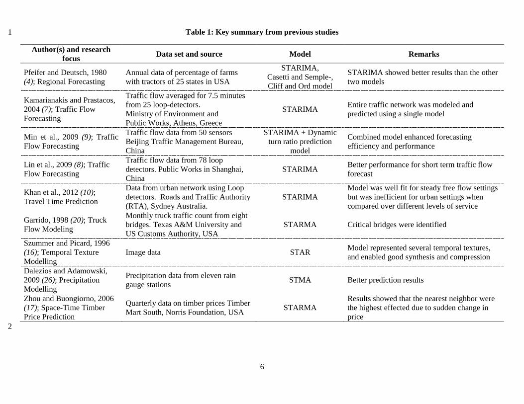
2. Literature Review 30

The space–time autoregressive moving average (STARMA) model class was introduced by 31

Pfeifer and Deutsch (3,4,5) in the early 1980s. This model class in an extension of autoregressive 32

moving average (ARMA) model (6). Later space-time autoregressive integrated moving average 33

(STARIMA) models were developed and used by researchers in their studies for forecasting as 34

well as analysis purposes. These models are used in several research areas such as traffic 35

engineering, economics, agricultural systems, biological system, ecology, neurological science, 36

etc. STARIMA models are used to describe, analyze, and forecast a set of N observable time 37

series. Space-time models best represent interaction among the neighboring regions of a system 38

by considering the spatial correlation among the regions. Such models attempt to describe the 39

dependencies between the regions of a systems across space and time. 40

Studying the relation and influence of neighbors with each other in a defined system has been an 41

important research area for the last two decades. Several studies have been conducted in the past 42

based on space-time modeling of time series data. Pfeifer and Deutsch (4) used the STARIMA 43

model to demonstrate prediction efficiency. Kamarianakis and Prastacos (7) developed 44

4

STARIMA models using traffic data obtained at different places in Athens (Greece) to predict 1

the space-time stationary traffic flow and assess the impact on other regions of the network. Lin 2

et al., (8) conducted similar studies for predicting the short-time interval traffic volume 3

prediction in Shanghai. The study showed that the model can be used to estimate a non-linear 4

function. Min et al., (9) forecasted short-time traffic flow on urban intersections in Beijing, 5

China with a combinations of STARIMA model and dynamic turn ratio prediction model. This 6

combination of models helped in enhancing the efficiency and the forecasting performance. In a 7

recent study, Khan et al., (10) studied the performance of STARIMA models in predicting the 8

travel times for dense and highly varying road traffic networks in Sydney, Australia. The 9

performance of the developed STARMA model was later analyzed for six Levels of Services 10

(LOS) of the roads. 11

Reynolds and Madden (11) summarized the theory of spatial-temporal correlation analysis on a 12

spatial-temporal dataset. The dataset consisted of temporal data of disease spread over a spatial 13

lattice structure, which was used for description of epidemics development. Madden et al., (12) 14

used STARIMA process to model the tobacco virus epidemics across six different fields in 15

Kentucky, USA. Epperson (13) used ecological data to characterize the genetic population and 16

estimate migration rates based on space time correlations. Soni et al., (14) used intervention 17

analysis and STARMA modeling to develop a method to remove the interfering signals present 18

in fetal bio-magnetic signals. 19

STARMA modeling process is also used for water resources planning and management. 20

Dalezios and Adamowski(15) developed a spatio–temporal moving average (STMA) 21

precipitation model to analyze the regional meteorology and hydrology in rural watersheds. The 22

STMA model was identified as the best fit to the hydrology dataset. Szummer and Picard (16) 23

used spatial temporal autoregressive (STAR) model to model the image sequences of temporal 24

textures (i.e., textures with motion). It is used in recognition and synthesis since a pixel can be 25

generated as a combination of its neighbor pixels lagged in space and time. 26

Zhou and Buongiorno(17) developed a space-time econometric model for pine saw timber price 27

predictions for 21 neighboring regions in southern USA. The researchers also performed an 28

impulse response analysis to see if the prices are globally integrated. Niu and Tiao(18) modeled 29

the satellite ozone data using STAR model. The satellite data was analyzed on a fixed latitude, 30

which takes into account the temporal and longitudinal dependence of the observations. The 31

space-time regression models are applied for trend assessment of monthly column ozone for each 32

of the subdivided geographical blocks. Giacinto(19) developed a generalized space-time model 33

to improve the model’s ability to cope with the spatial features of data. It also includes an 34

application to regional unemployment analysis in Italy aimed at evaluating how a shock in a 35

region propagates spatially extent in relation to unemployment and finding the degree of spatial 36

heterogeneity in the process parameters. A summary from some of the above discussed studies is 37

presented in Table 1. 38

Application of spatial temporal modeling mechanism on freight flow is limited to a study 39

conducted by Garrido(20). Garrido analyzed space time interaction between truck flows through 40

eight bridges located on Texas-Mexico Border. Also recent studies related to Indian major port 41

systems are limited to Sahu and Patil(21), Sahu et al.,(22), and Patil and Sahu(1,23). Their study 42

mainly focused on estimating freight demand for Indian ports using regression and time series 43

modeling techniques. Their study models include ARIMA, SARIMA, VAR, and dynamic 44

regression models. However, their models did not consider the effect of neighboring port freight 45

5

demand while estimating the demand for a subject port. In other words, their research did not 1

analyze the spatial interaction between freight flows at the study ports. In the present research, 2

the spatial temporal variation in freight flow at a neighbor port is considered while modeling the 3

freight at a specific port. 4

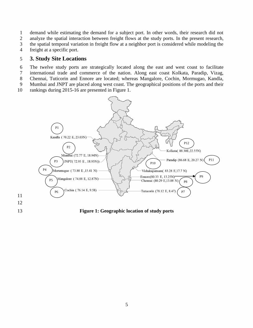
3. Study Site Locations 5

The twelve study ports are strategically located along the east and west coast to facilitate 6

international trade and commerce of the nation. Along east coast Kolkata, Paradip, Vizag, 7

Chennai, Tuticorin and Ennore are located; whereas Mangalore, Cochin, Mormugao, Kandla, 8

Mumbai and JNPT are placed along west coast. The geographical positions of the ports and their 9

rankings during 2015-16 are presented in Figure 1. 10

11

12

Figure 1: Geographic location of study ports13

P1

P11 P3

P2

P10

P12

P8

P7

P5 P9

P6

P4

6

Table 1: Key summary from previous studies 1

Author(s) and research

focus Data set and source Model Remarks

Pfeifer and Deutsch, 1980

(4); Regional Forecasting

Annual data of percentage of farms

with tractors of 25 states in USA

STARIMA,

Casetti and Semple-,

Cliff and Ord model

STARIMA showed better results than the other

two models

Kamarianakis and Prastacos,

2004 (7); Traffic Flow

Forecasting

Traffic flow averaged for 7.5 minutes

from 25 loop-detectors.

Ministry of Environment and

Public Works, Athens, Greece

STARIMA Entire traffic network was modeled and

predicted using a single model

Min et al., 2009 (9); Traffic

Flow Forecasting

Traffic flow data from 50 sensors

Beijing Traffic Management Bureau,

China

STARIMA + Dynamic

turn ratio prediction

model

Combined model enhanced forecasting

efficiency and performance

Lin et al., 2009 (8); Traffic

Flow Forecasting

Traffic flow data from 78 loop

detectors. Public Works in Shanghai,

China

STARIMA Better performance for short term traffic flow

forecast

Khan et al., 2012 (10);

Travel Time Prediction

Data from urban network using Loop

detectors. Roads and Traffic Authority

(RTA), Sydney Australia.

STARIMA

Model was well fit for steady free flow settings

but was inefficient for urban settings when

compared over different levels of service

Garrido, 1998 (20); Truck

Flow Modeling

Monthly truck traffic count from eight

bridges. Texas A&M University and

US Customs Authority, USA

STARMA Critical bridges were identified

Szummer and Picard, 1996

(16); Temporal Texture

Modelling

Image data STAR Model represented several temporal textures,

and enabled good synthesis and compression

Dalezios and Adamowski,

2009 (26); Precipitation

Modelling

Precipitation data from eleven rain

gauge stations STMA Better prediction results

Zhou and Buongiorno, 2006

(17); Space-Time Timber

Price Prediction

Quarterly data on timber prices Timber

Mart South, Norris Foundation, USA STARMA

Results showed that the nearest neighbor were

the highest effected due to sudden change in

price

2

7

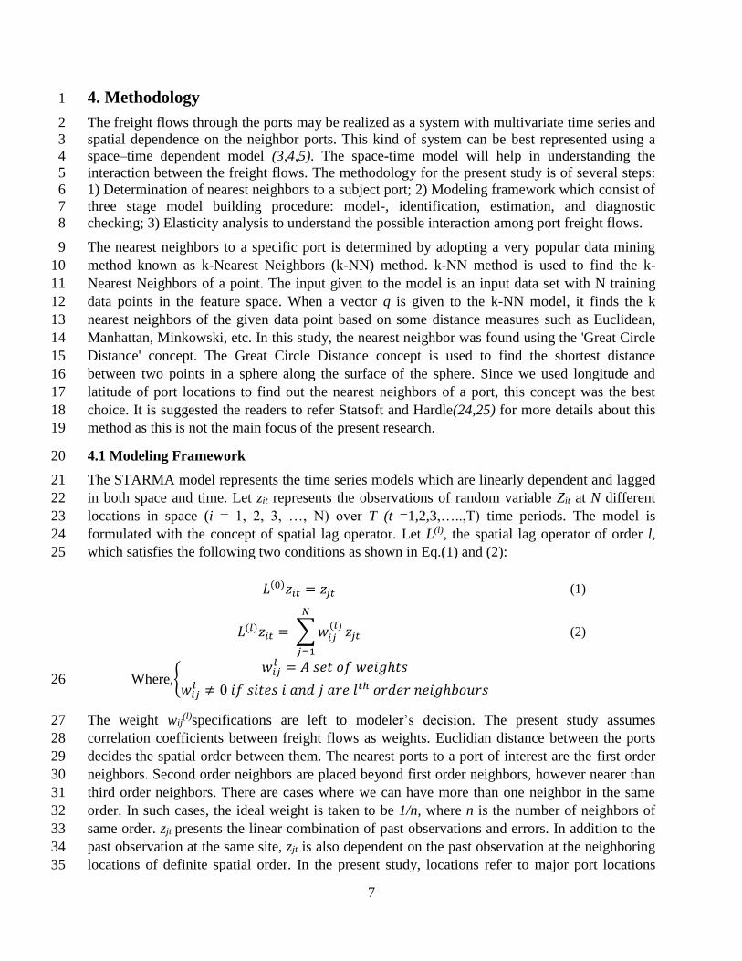
4. Methodology 1

The freight flows through the ports may be realized as a system with multivariate time series and 2

spatial dependence on the neighbor ports. This kind of system can be best represented using a 3

space–time dependent model (3,4,5). The space-time model will help in understanding the 4

interaction between the freight flows. The methodology for the present study is of several steps: 5

1) Determination of nearest neighbors to a subject port; 2) Modeling framework which consist of 6

three stage model building procedure: model-, identification, estimation, and diagnostic 7

checking; 3) Elasticity analysis to understand the possible interaction among port freight flows. 8

The nearest neighbors to a specific port is determined by adopting a very popular data mining 9

method known as k-Nearest Neighbors (k-NN) method. k-NN method is used to find the k-10

Nearest Neighbors of a point. The input given to the model is an input data set with N training 11

data points in the feature space. When a vector q is given to the k-NN model, it finds the k 12

nearest neighbors of the given data point based on some distance measures such as Euclidean, 13

Manhattan, Minkowski, etc. In this study, the nearest neighbor was found using the 'Great Circle 14

Distance' concept. The Great Circle Distance concept is used to find the shortest distance 15

between two points in a sphere along the surface of the sphere. Since we used longitude and 16

latitude of port locations to find out the nearest neighbors of a port, this concept was the best 17

choice. It is suggested the readers to refer Statsoft and Hardle(24,25) for more details about this 18

method as this is not the main focus of the present research. 19

4.1 Modeling Framework 20

The STARMA model represents the time series models which are linearly dependent and lagged 21

in both space and time. Let zit represents the observations of random variable Zit at N different 22

locations in space (i = 1, 2, 3, …, N) over T (t =1,2,3,…..,T) time periods. The model is 23

formulated with the concept of spatial lag operator. Let L(l), the spatial lag operator of order l, 24

which satisfies the following two conditions as shown in Eq.(1) and (2): 25

𝐿(0)𝑧𝑖𝑡 = 𝑧𝑗𝑡 (1)

𝐿(𝑙)𝑧𝑖𝑡 = ∑ 𝑤𝑖𝑗(𝑙)

𝑁

𝑗=1

𝑧𝑗𝑡 (2)

Where,{𝑤𝑖𝑗

𝑙 = 𝐴 𝑠𝑒𝑡 𝑜𝑓 𝑤𝑒𝑖𝑔ℎ𝑡𝑠

𝑤𝑖𝑗𝑙 ≠ 0 𝑖𝑓 𝑠𝑖𝑡𝑒𝑠 𝑖 𝑎𝑛𝑑 𝑗 𝑎𝑟𝑒 𝑙𝑡ℎ 𝑜𝑟𝑑𝑒𝑟 𝑛𝑒𝑖𝑔ℎ𝑏𝑜𝑢𝑟𝑠

26

The weight wij(l)specifications are left to modeler’s decision. The present study assumes 27

correlation coefficients between freight flows as weights. Euclidian distance between the ports 28

decides the spatial order between them. The nearest ports to a port of interest are the first order 29

neighbors. Second order neighbors are placed beyond first order neighbors, however nearer than 30

third order neighbors. There are cases where we can have more than one neighbor in the same 31

order. In such cases, the ideal weight is taken to be 1/n, where n is the number of neighbors of 32

same order. zjt presents the linear combination of past observations and errors. In addition to the 33

past observation at the same site, zjt is also dependent on the past observation at the neighboring 34

locations of definite spatial order. In the present study, locations refer to major port locations 35

8

with respective latitude and longitude. With these definitions, the STARMA (3,7) model is 1

presented in Eq.(3). 2

𝑧𝑖𝑡 = ∑ ∑ 𝜙𝑘𝑙 ∑ 𝑤𝑖𝑗(𝑙)

𝑧𝑗𝑡−𝑘

𝑁

𝑗=1

𝜆𝑘

𝑙=0

+ ∑ ∑ 𝜃𝑘𝑙 ∑ 𝑤𝑖𝑗(𝑙)

𝑎𝑗𝑡−𝑘

𝑁

𝑗=1

𝑚𝑘

𝑙=0

𝑞

𝑘=1

+ 𝑎𝑖𝑡 (3)

𝑝

𝑘=1

(

Where zit is the freight flow through the port i during quarter t, ait is the random normal 3

error associated with port i during quarter t such that the following condition is satisfied as 4

shown in Eq. (4). 5

𝛦[𝑎𝑖𝑡𝑎𝑗𝑡+𝑠] = {𝜎2 𝑖 = 𝑗, 𝑠 = 00 𝑂𝑡ℎ𝑒𝑟𝑤𝑖𝑠𝑒

(4)

Where, E[.] =Expected value 6

p= autoregression order 7

q= moving average order 8

λk= spatial order of the kth autoregressive term 9

mk= spatial order of the kth moving average term 10

N= number of spatial units (ports) 11

ϕkl and θkl are the parameters 12

wij(l)= level of interaction between the ports i and j 13

This model is referred as STARMA (pλ1,λ2,…λp, qm1,m2,…mq). Two special cases of STARMA exists 14

when either p=0 or q=0. The model becomes a STAR model if q=0. 15

𝑧𝑖𝑡 = ∑ ∑ 𝜙𝑘𝑙 ∑ 𝑤𝑖𝑗(𝑙)

𝑧𝑗𝑡−𝑘

𝑁

𝑗=1

𝜆𝑘

𝑙=0

+ 𝑎𝑖𝑡

𝑝

𝑘=1

(5)

The model shown is Eq.(5) is referred to as STAR(pλ1,λ2,…λp) model. Similarly, for p=0, only 16

moving average terms remain and the model becomes STMA(qm1,m2,..,mq) model as presented 17

through Eq.(6). 18

𝑧𝑖𝑡 = 𝑎𝑖𝑡 + ∑ ∑ 𝜃𝑘𝑙 ∑ 𝑤𝑖𝑗(𝑙)

𝑎𝑗𝑡−𝑘

𝑁

𝑗=1

𝑚𝑘

𝑙=0

𝑞

𝑘=1

(6)

4.1.1 Model Identification 19

The first stage of the three-stage model building procedure is the model identification from the 20

dataset. In the case of univariate time series models, we identify the best suited model from 21

autocorrelation and partial-autocorrelation functions. However, in the case of space-time models 22

the N2 possible cross-variances between all possible pairs of locations are combined to obtain 23

proposed models. Analogous to the univariate time series models, the space-time models are 24

identified using two-dimensional space-time autocorrelation function (STACF) and space-time 25

9

partial-autocorrelation function (STPACF). Possible model orders (p,q) for the three subclasses 1

of space-time models (STAR, STMA, STARMA) are determined by checking the pattern of 2

STACF and STPACF. 3

4.1.2 Model Estimation 4

Once the model is identified, then the optimal estimates for AR(ϕ) and MA(θ) is done using 5

maximum likelihood estimation procedure (4). Unlike STMA and STARMA models, the STAR 6

model parameters are estimated on the principle of linear regression theory (i.e., using 7

conditional maximum likelihood estimation to find the least residual sum of squares). However, 8

STMA and STARMA models are non-linear in nature. Hence, a 'gradient method’ is used which 9

uses Taylor’s Expansion to linearize the non-linear model. 10

4.1.3 Diagnostic Checking 11

Once a suitable model is selected and parameters are estimated, diagnostic checks are performed 12

on the model to check if it exemplifies the data. Normally, a model may fail in two ways. Firstly, 13

it has to be checked whether the residual of the fitted model has any significant correlation. Any 14

observed correlation in the residuals is not desired. If the fitted model adequately represents the 15

data should be distributed normally with mean zero, the variance-covariance matrix should be 16

spherical. Secondly, the model can become complex. Hence, it is important to check if the 17

parameters are statistically significant. 18

4.2 Elasticity Analysis 19

After the model is estimated and checked for statistical significance, the freight flows at different 20

ports can be examined through elasticity analysis. In other words, the interaction among ports 21

can be analyzed by determining the cross elasticities. The cross elasticities are used to 22

understand the interaction between a particular port and its’ neighbors. It explains how the 23

freight flow at a port is affected by the changes in freight flows in its neighbor ports. This, in 24

turn, gives us an insight into whether the two nearest ports are competing or complementing. If 25

the cross elasticity between two ports is negative, it means that the two ports are competing with 26

each other to attract freight. If it is positive, it means that the freight volume of the target port 27

increases/decreases with the increase/decrease in the volume of the neighbor port (i.e., they 28

complement each other). Generally, the elasticity function is defined as follows. 29

𝜖𝑙(𝐴 𝐵⁄ ) = (𝜕𝐴 𝜕𝐵)⁄ ∗ (𝐵 𝐴)⁄ ; Where, A, B are two continuous and differential 30

variables. 31

The change in the freight flow of a port i in quarter t when the freight flow at port j is changed in 32

quarter t-q, is given by Eq. (7) 33

𝜖𝑙 (𝑧𝑖𝑡

𝑧𝑗𝑡−𝑞) =

𝜕𝑧𝑖𝑡

𝜕𝑧𝑗𝑡−𝑞

𝑧𝑗𝑡−𝑞

𝑧𝑖𝑡 (7)

Case 1: Direct elasticity: In case i=j, the Eq. (7) referred as direct elasticity. Taking spatial order 34

is taken as 1 (l =1) and applying Eq. (7) is to (3), the Eq.(7) gets converted to Eq.(8): 35

𝜖𝑙 (𝑧𝑖𝑡

𝑧𝑖𝑡−𝑞) = 𝛼𝑠

𝑧𝑖𝑡−𝑞

𝑧𝑖𝑡 (8)

10

Case 2: Cross elasticity: In case i ≠ j, and applying Eq. (7) to (3) with spatial order 1, the Eq. (7) 1

becomes Eq. (9): 2

𝜖𝑙 (𝑧𝑖𝑡

𝑧𝑗𝑡−𝑞) = 𝛼𝑠𝑤𝑖𝑗

𝑧𝑗𝑡−𝑞

𝑧𝑖𝑡 𝑓𝑜𝑟 𝑖 ≠ 𝑗 (9)

4.3 Data 3

This dataset consists of quarterly freight flows for twelve major ports of India between the 4

periods of Quarter – I, 2001-2002 to Quarter – III, 2015-2016. The freight flows considered in 5

this study consist of both inward and outward freight flows. Some key statistics related to port 6

freight flow series are presented in Table 2. The port which handles the highest volume of freight 7

in eastern and western coasts are Vizag and Kandla respectively. Mormugao port has a very high 8

coefficient of variation (around 59%) because of the seasonal variation in the freight handled by 9

the port. The ports in the western coast and eastern coast handle almost equal quarterly freight by 10

volume, accounting for 50.1% (60.067 million tons) and 49.9% (59.817 million tons) 11

respectively. The variability of freight volume for five of the six ports in the western coast lies 12

between 19% and 32%, except for Mormugao whose variability has already been explained. 13

Similarly, the variability for ports in the eastern coast lies between 17% and 34%, except for 14

Ennore which has a high variability of 51.5%. The trend in the freight volume for most of the 15

ports show an increasing trend, though the gradient for each of them varies. 16

Table 2: Basic statistics for the freight flows through major ports in India 17

Port Average 1(tons) Std. Dev. CV 2 Minimum Maximum

Kandla (P1) 17.321 5.399 0.312 9.044 25.767

Mumbai (P2) 10.139 3.151 0.311 5.883 16.335

JNPT (P3) 12.701 3.736 0.294 5.444 16.997

Mormugao (P4) 7.529 4.416 0.587 1.353 19.208

Mangalore (P5) 8.088 1.631 0.202 3.788 10.289

Cochin (P6) 4.289 0.829 0.193 2.547 5.790

Tuticorin (P7) 5.750 1.701 0.296 3.048 9.466

Chennai (P8) 12.515 2.334 0.186 7.846 16.752

Ennore (P9) 3.799 1.955 0.515 1.418 8.25

Vizag (P10) 14.368 1.992 1.992 9.910 17.643

Paradip (P11) 11.935 4.048 0.339 5.419 19.604

Kolkata (P12) 11.450 1.946 0.170 7.320 15.100 1Average quarterly freight flow (million tons) 18 2Coefficient of variation (standard deviation/average) 19

Number of observations: 59 (Quarter – I, 2001-2002 to Quarter – III, 2015-2016) 20

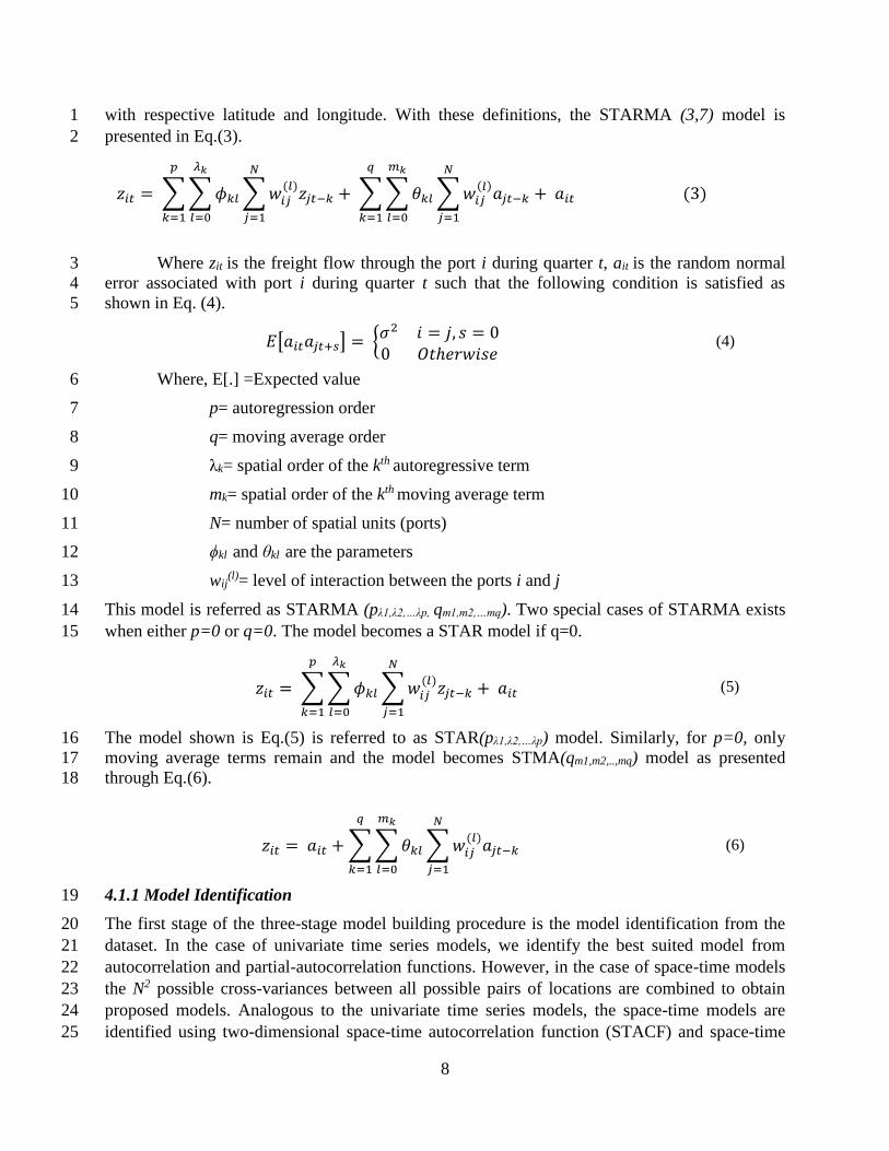
5. Model Development and Estimation Process 21

The spatial-temporal model development and estimation was carried out in several steps using 22

statistical computing language R3.2.3. The model orders were identified using STACF and 23

11

STPACF plots. The STACF plots showed tails cutoff and STPACF appeared to be cut off after 1 1

time lag at 1 spatial lag. Therefore, the model is identified as STARMA (1,0,1) or STAR (1,1). 2

An algorithm was developed to estimate the model using ‘starma’ packages available with R 3

software. The algorithm is explained in the subsequent subsection. 4

4.1 Modeling Algorithm 5

The STARMA model development follows a three-stage iterative model building process 6

consisting of model identification, estimation and diagnostic checking of the selected model. The 7

steps involved in achieving the best fitted model is explained in the following sub-sections. 8

4.2.1 Steps of the Algorithm 9

The model was developed using ‘starma’ and ‘spdep’ package of R program. The ‘starma’ 10

package, developed by Felix Cheysson, helps in identifying, estimating and diagnosing space-11

time dependent STARMA models. 'spdep' package creates spatial weights matrix objects. The 12

several steps in model development are as follows. 13

Step 1: Develop a coordinate matrix: 14

A matrix is developed with each row as a port location consisting of longitude and latitude as 15

columns. Then the point coordinates are plotted. The coordinates for all the major ports have 16

been extracted with the help of Google Map. The longitude and latitude for each port is 17

presented below. 18

Port Longitude Latitude Port Longitude Latitude Port Longitude Latitude

Kandla 70.22oE 23.03oN Mangalore 74.88oE 12.87oN Ennore 80.33oE 13.25oN

Mumbai 72.77oE 18.94oN Cochin 76.14oE 9.58oN Vizag 83.28oE 17.70oN

JNPT 72.95oE 18.95oN Tuticorin 78.12oE 8.47oN Paradip 86.68oE 20.27oN

Mormugao 73.80oE 15.41oN Chennai 80.29oE 13.08oN Kolkata 88.30oE 22.55oN

Step 2: Identify the nearest neighbor: 19

The nearest neighbor for each of the ports is determined using k-nearest neighbor method, where 20

k=1 in this case. The nearest neighbor is then used to give spatial weight in the weight matrix. A 21

matrix showing each of the ports and their respective neighbors is obtained using “knearneigh” 22

function of the ‘spdep’ package. The list of all the ports and their respective nearest neighbor 23

port are shown below. 24

Port Nearest port Port Nearest port Port Nearest port

Kandla Mumbai Mangalore Mormugao Ennore Chennai

Mumbai JNPT Cochin Tuticorin Vizag Paradip

JNPT Mumbai Tuticorin Cochin Paradip Kolkata

Mormugao Mangalore Chennai Ennore Kolkata Paradip

Step 3: Determine correlation coefficient for nearest neighbor ports: 25

Correlation between each of the pair of nearest neighbor ports is obtained using ‘cor’ function of 26

R package. The Pearson correlation coefficients were calculated using the port freight data for all 27

the paired ports. 28

12

Step 4: Create weight matrices: 1

Zeroth order weight matrix is the matrix which shows how a given port is influenced by its zeroth 2

order neighbor (i.e., itself). A diagonal matrix with same size as the number of ports is created. 3

Table 3 shows the first order weight matrix which shows how a given port is influenced by its 4

nearest neighbor. Higher order matrices were also attempted to consider in the modeling process, 5

however, the model statistics were not found to be significant. Therefore, only first order matrix 6

is presented here. The matrix is created with each row consisting of all values as zero except the 7

nearest neighbor column which is filled with correlation coefficient value. Since the spatial order 8

(l) is taken as 1 in our case, only zeroth and first order weight matrix are created. Such weight 9

matrices represent the interaction between the ports according to the modeler’s choice. 10

Correlation matrix was taken to be the first order weight matrix since it gives the linear 11

dependence between the nearest neighbor ports. The spatial lag operator is taken in this study as 12

follows: 13

𝑤𝑖𝑗 = {𝜌𝑖𝑗 ∀ 𝑖 ≠ 𝑗

0 𝑖 = 𝑗

Where, ρij is the Pearson’s correlation coefficient of freight flows at two nearest neighbor ports i 14

and j. 15

Table 3: First order weight matrix (W(1)) 16

P1 P2 P3 P4 P5 P6 P7 P8 P9 P10 P11 P12

P1 0 0.799 0 0 0 0 0 0 0 0 0 0

P2 0 0 0.731 0 0 0 0 0 0 0 0 0

P3 0 0.731 0 0 0 0 0 0 0 0 0 0

P4 0 0 0 0 -0.012 0 0 0 0 0 0 0

P5 0 0 0 -0.012 0 0 0 0 0 0 0 0

P6 0 0 0 0 0 0 0.899 0 0 0 0 0

P7 0 0 0 0 0 0.899 0 0 0 0 0 0

P8 0 0 0 0 0 0 0 0 0.209 0 0 0

P9 0 0 0 0 0 0 0 0.209 0 0 0 0

P10 0 0 0 0 0 0 0 0 0 0 0.631 0

P11 0 0 0 0 0 0 0 0 0 0 0 0.289

P12 0 0 0 0 0 0 0 0 0 0 0.289 0

Step 5: Center and scale the dataset: 17

The data is centered using “stcenter” method of the STARMA package in R. The data is centered 18

and scaled using this method to avoid any intercept tem in the model. In “stcenter” function, the 19

data is centered globally since it is considered all points come from a single process. 20

21

13

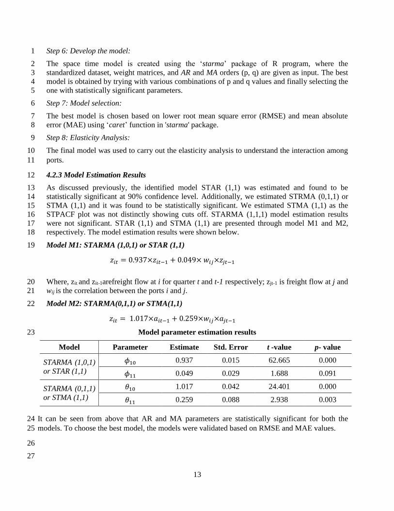
Step 6: Develop the model: 1

The space time model is created using the ‘starma’ package of R program, where the 2

standardized dataset, weight matrices, and AR and MA orders (p, q) are given as input. The best 3

model is obtained by trying with various combinations of p and q values and finally selecting the 4

one with statistically significant parameters. 5

Step 7: Model selection: 6

The best model is chosen based on lower root mean square error (RMSE) and mean absolute 7

error (MAE) using ‘caret’ function in 'starma' package. 8

Step 8: Elasticity Analysis: 9

The final model was used to carry out the elasticity analysis to understand the interaction among 10

ports. 11

4.2.3 Model Estimation Results 12

As discussed previously, the identified model STAR (1,1) was estimated and found to be 13

statistically significant at 90% confidence level. Additionally, we estimated STRMA (0,1,1) or 14

STMA (1,1) and it was found to be statistically significant. We estimated STMA (1,1) as the 15

STPACF plot was not distinctly showing cuts off. STARMA (1,1,1) model estimation results 16

were not significant. STAR (1,1) and STMA (1,1) are presented through model M1 and M2, 17

respectively. The model estimation results were shown below. 18

Model M1: STARMA (1,0,1) or STAR (1,1) 19

𝑧𝑖𝑡 = 0.937×𝑧𝑖𝑡−1 + 0.049× 𝑤𝑖𝑗×𝑧𝑗𝑡−1

Where, zit and zit-1arefreight flow at i for quarter t and t-1 respectively; zjt-1 is freight flow at j and 20

wij is the correlation between the ports i and j. 21

Model M2: STARMA(0,1,1) or STMA(1,1) 22

𝑧𝑖𝑡 = 1.017×𝑎𝑖𝑡−1 + 0.259×𝑤𝑖𝑗×𝑎𝑗𝑡−1

Model parameter estimation results 23

Model Parameter Estimate Std. Error t -value p- value

STARMA (1,0,1)

or STAR (1,1)

𝜙10 0.937 0.015 62.665 0.000

𝜙11 0.049 0.029 1.688 0.091

STARMA (0,1,1)

or STMA (1,1)

𝜃10 1.017 0.042 24.401 0.000

𝜃11 0.259 0.088 2.938 0.003

It can be seen from above that AR and MA parameters are statistically significant for both the 24

models. To choose the best model, the models were validated based on RMSE and MAE values. 25

26

27

14

4.2.4 Model Performance 1

The models performances were validated through RMSE and MAE values. They are defined in 2

Eq.(10) and Eq.(11). 3

𝑀𝐴𝐸 = 1

𝑛∑|𝑌𝑜𝑏𝑠,𝑡 − 𝑌𝑚𝑜𝑑𝑒𝑙,𝑡|

𝑛

𝑡=1

(10)

4

𝑅𝑀𝑆𝐸 = √∑ (𝑌𝑜𝑏𝑠,𝑡 − 𝑌𝑚𝑜𝑑𝑒𝑙,𝑡)2𝑛

𝑡=1

𝑛 (11)

Where, n= number of quarters, Yobs,k and Ymodel,k are the observed and modeled freight flow for 5

the tth quarter, respectively. 6

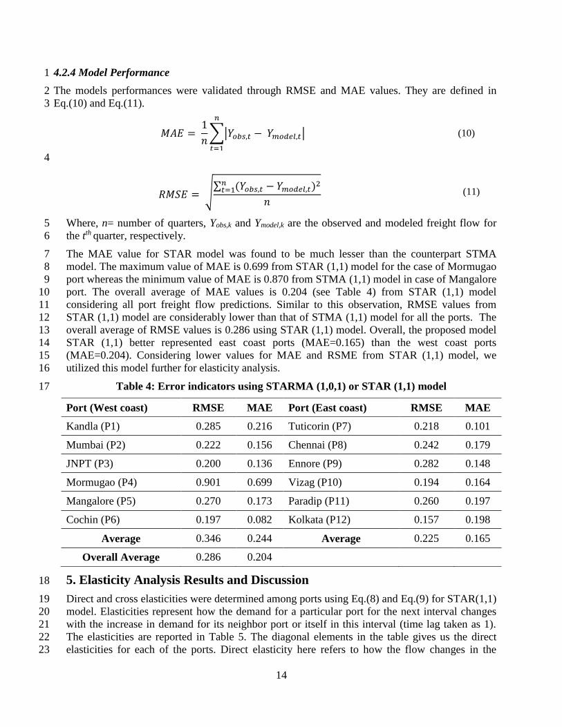
The MAE value for STAR model was found to be much lesser than the counterpart STMA 7

model. The maximum value of MAE is 0.699 from STAR (1,1) model for the case of Mormugao 8

port whereas the minimum value of MAE is 0.870 from STMA (1,1) model in case of Mangalore 9

port. The overall average of MAE values is 0.204 (see Table 4) from STAR (1,1) model 10

considering all port freight flow predictions. Similar to this observation, RMSE values from 11

STAR (1,1) model are considerably lower than that of STMA (1,1) model for all the ports. The 12

overall average of RMSE values is 0.286 using STAR (1,1) model. Overall, the proposed model 13

STAR (1,1) better represented east coast ports (MAE=0.165) than the west coast ports 14

(MAE=0.204). Considering lower values for MAE and RSME from STAR (1,1) model, we 15

utilized this model further for elasticity analysis. 16

Table 4: Error indicators using STARMA (1,0,1) or STAR (1,1) model 17

Port (West coast) RMSE MAE Port (East coast) RMSE MAE

Kandla (P1) 0.285 0.216 Tuticorin (P7) 0.218 0.101

Mumbai (P2) 0.222 0.156 Chennai (P8) 0.242 0.179

JNPT (P3) 0.200 0.136 Ennore (P9) 0.282 0.148

Mormugao (P4) 0.901 0.699 Vizag (P10) 0.194 0.164

Mangalore (P5) 0.270 0.173 Paradip (P11) 0.260 0.197

Cochin (P6) 0.197 0.082 Kolkata (P12) 0.157 0.198

Average 0.346 0.244 Average 0.225 0.165

Overall Average 0.286 0.204

5. Elasticity Analysis Results and Discussion 18

Direct and cross elasticities were determined among ports using Eq.(8) and Eq.(9) for STAR(1,1) 19

model. Elasticities represent how the demand for a particular port for the next interval changes 20

with the increase in demand for its neighbor port or itself in this interval (time lag taken as 1). 21

The elasticities are reported in Table 5. The diagonal elements in the table gives us the direct 22

elasticities for each of the ports. Direct elasticity here refers to how the flow changes in the 23

15

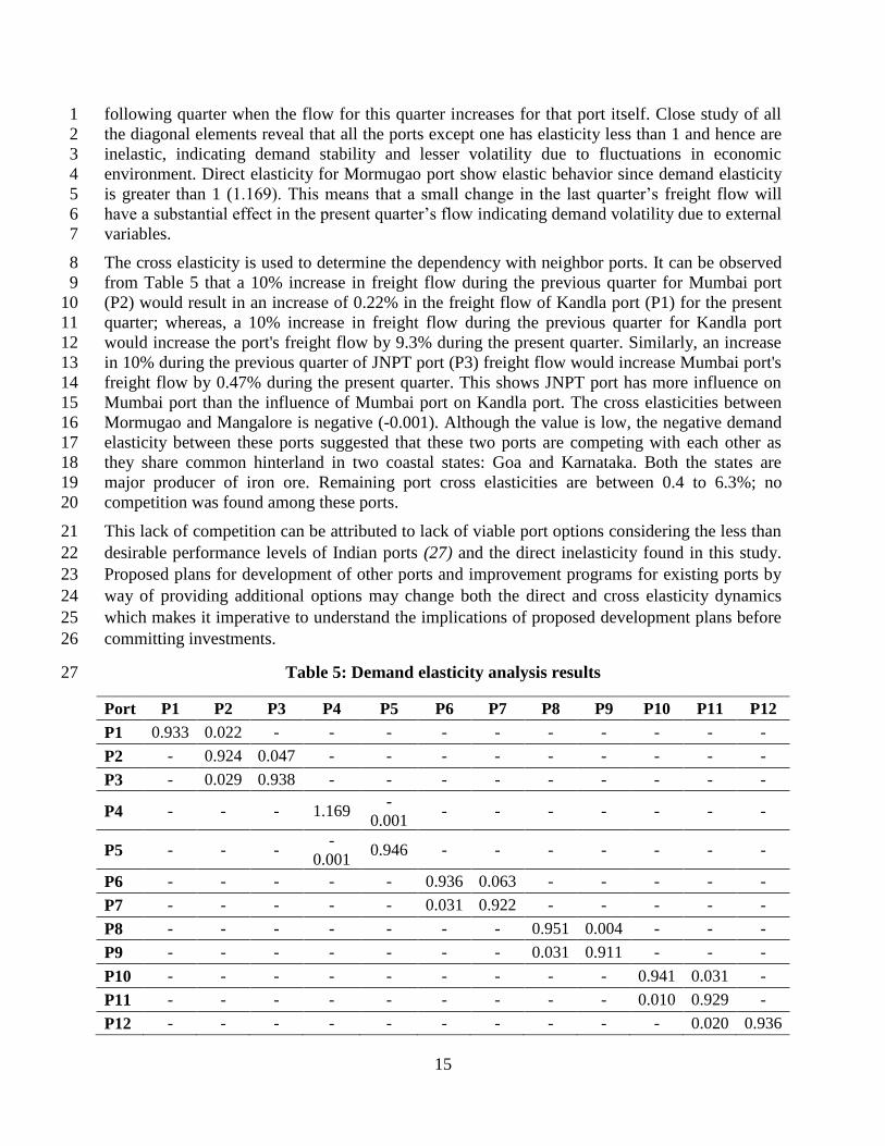
following quarter when the flow for this quarter increases for that port itself. Close study of all 1

the diagonal elements reveal that all the ports except one has elasticity less than 1 and hence are 2

inelastic, indicating demand stability and lesser volatility due to fluctuations in economic 3

environment. Direct elasticity for Mormugao port show elastic behavior since demand elasticity 4

is greater than 1 (1.169). This means that a small change in the last quarter’s freight flow will 5

have a substantial effect in the present quarter’s flow indicating demand volatility due to external 6

variables. 7

The cross elasticity is used to determine the dependency with neighbor ports. It can be observed 8

from Table 5 that a 10% increase in freight flow during the previous quarter for Mumbai port 9

(P2) would result in an increase of 0.22% in the freight flow of Kandla port (P1) for the present 10

quarter; whereas, a 10% increase in freight flow during the previous quarter for Kandla port 11

would increase the port's freight flow by 9.3% during the present quarter. Similarly, an increase 12

in 10% during the previous quarter of JNPT port (P3) freight flow would increase Mumbai port's 13

freight flow by 0.47% during the present quarter. This shows JNPT port has more influence on 14

Mumbai port than the influence of Mumbai port on Kandla port. The cross elasticities between 15

Mormugao and Mangalore is negative (-0.001). Although the value is low, the negative demand 16

elasticity between these ports suggested that these two ports are competing with each other as 17

they share common hinterland in two coastal states: Goa and Karnataka. Both the states are 18

major producer of iron ore. Remaining port cross elasticities are between 0.4 to 6.3%; no 19

competition was found among these ports. 20

This lack of competition can be attributed to lack of viable port options considering the less than 21

desirable performance levels of Indian ports (27) and the direct inelasticity found in this study. 22

Proposed plans for development of other ports and improvement programs for existing ports by 23

way of providing additional options may change both the direct and cross elasticity dynamics 24

which makes it imperative to understand the implications of proposed development plans before 25

committing investments. 26

Table 5: Demand elasticity analysis results 27

Port P1 P2 P3 P4 P5 P6 P7 P8 P9 P10 P11 P12

P1 0.933 0.022 - - - - - - - - - -

P2 - 0.924 0.047 - - - - - - - - -

P3 - 0.029 0.938 - - - - - - - - -

P4 - - - 1.169 -

0.001 - - - - - - -

P5 - - - -

0.001 0.946 - - - - - - -

P6 - - - - - 0.936 0.063 - - - - -

P7 - - - - - 0.031 0.922 - - - - -

P8 - - - - - - - 0.951 0.004 - - -

P9 - - - - - - - 0.031 0.911 - - -

P10 - - - - - - - - - 0.941 0.031 -

P11 - - - - - - - - - 0.010 0.929 -

P12 - - - - - - - - - - 0.020 0.936

16

6. Conclusion 1

The correlation between the freight flows and interaction between the ports was expected to be 2

best represented by a space-time model. The quarterly time-series data obtained from the 12 3

major ports located along the east and west coast of India were used for analysis. The data were 4

analyzed through a newly proposed space-time model STAR (1,1,) with due consideration 5

towards understanding the influence of neighboring ports on a subject port. 6

Elasticity analysis of such a model revealed some interesting insights regarding the space-time 7

dependence of a port freight flow on nearest neighbor port. Direct elasticity analysis suggested 8

how the freight flow of a particular port in the present quarter is affected by the change in freight 9

flow of that port in the previous quarter. The direct elasticity values for all the major ports ranged 10

between 0.911 (Ennore) and 1.169 (Mormugao). This shows that the freight flows during the 11

current quarter are highly dependent on the volume of its earlier quarter period. Higher direct 12

elasticity value for Mormugao (1.169) indicated that the freight handled by the port in the present 13

quarter is significantly affected by the change in the freight handled by the port in the previous 14

quarter. Cross elasticity values on the other hand ranged between -0.001 and 0.063. The variation 15

between the two extremes is almost different by a factor of 6, which is significant. It is quite high 16

when compared to the direct elasticities because cross elasticity, unlike direct elasticity, is 17

influenced by both space and time. Negative values of cross elasticities between Mormugao and 18

Mangalore indicate that these two ports compete with each other for attracting freight from their 19

common hinterland existence in two coastal states: Goa and Karnataka. 20

The freight flow forecasting of ports has been done till now using its past freight flow data 21

without considering the effects of its neighbor ports. When forecasting the freight flows, it is 22

therefore important to know if the past and current freight flow in neighbor ports can help make 23

the forecasting even better. The proposed models can be used for short-term forecasting of 24

freight flows through the major ports and assessing the impact of freight flow changes from one 25

port to the nearest neighboring ports. It is expected that this study will help port authorities and 26

policy makers for holistic development of port system by making right investments in required 27

locations to promote balanced development. It has also implications towards formulating policies 28

on port development considering Government of India's preferred mode of choice for 29

infrastructure development is PPP, and policy formulation for this mode of development is 30

required to address competition concerns considering the high sunk cost associated with ports 31

development. 32

Acknowledgement 33

Thank to Ministry of Shipping, Mumbai Port Trust and Paradip Port Trust for the data used in 34

this study. 35

References 36

1. Patil, G., and Sahu, P. (2016), “Simultaneous dynamic demand estimation models for major 37

seaports in India", Transportation Letters, DOI:10.1080/19427867.2016.1203582 38

2. Maritime India Summit (2016) <http://www.maritimeinvest.in/new-port-development> (last 39

accessed on July 22, 2016) 40

3. Pfeifer P.E., Deutsch S.J.,(1980), "A three stage iterative model building procedure for space-41

time modeling, Technometrics, Vol.22(1):35-47 42

17

4. Pfeifer P.E. and Deutsch S.J., (1980)"A STARIMA model building procedure with application 1

to description and regional forecasting", Transactions of the Institute of British Geographers, 2

New Series, Vol.5( 3): 330-349 3

5. Pfeifer P.E. and Deutsch S.J. (1980), "Identification and interpretation of first order space-time 4

ARMA models", Technometrics, Vol.22(3): 397-408 5

6. Box, G.E.P. and Jenkins, G.M. (1970), "Time series analysis, forecasting and control", San 6

Francisco: Holden-Day 7

7. Kamarianakis Y., Prastacos P., (2005),"Space–time modeling of traffic flow", Computer & 8

Geosciences, Vol.31: 119-133 9

8. Lin, Huang, Zhu, Wang (2009), "The application of space – time ARIMA on traffic flow 10

forecasting", Proceedings of the Eighth International Conference on Machine Learning and 11

Cybernetics, Baoding, China, July, 12-15 12

9. Min X., Hu J., Chen Q., Zhang T., Zhang T., and Zhang Y., (2009),"Short term traffic flow 13

forecasting of urban network based on dynamic STARIMA model", Proceedings of the 12th 14

International IEEE Conference on Intelligent Transportation Systems, St. Louis, USA 15

10. Khan, Landfeldt and Dhamdhere, (2012), "Predicting travel times in dense and highly 16

varying road traffic networks using STARIMA models", Technical Report 685, School of 17

Information Technologies, The University of Sydney 18

11. Reynolds, K. M., and Madden, L. V., (1987), "Analysis of epidemics using spatio-temporal 19

autocorrelation", Phytopathology, Vol.78: 240-246. 20

12. Madden L.V., Reynolds K.M., Pirone T.P. and Raccah B., (1988), "Modeling of tobacco 21

virus epidemics as spatio-temporal autoregressive integrated moving average process", 22

Phytopathology, Vol.78:1361-1366 23

13. Epperson B.K., (2000), "Spatial and space-time correlations in ecological models", 24

Ecological Modeling, Vol.132: 63-76 25

14. Soni P., Chan Y., Eswaran H., Wilson J.D., Murphy P. and Lowery C.L., (2007), "Spatio-26

temporal analysis of fetal bio-magnetic signals", Journal of Neuroscience Methods, Vol.162: 27

333-345 28

15. Dalezios, N. R., and Adamowski, K., (1995), "Spatio-temporal precipitation modelling in 29

rural watersheds", Hydrological Sciences Journal, Vol.40(5):553-568, DOI: 30

10.1080/02626669509491444 31

16. Szummer, M., Picard, R.W., "Temporal texture modelling", Technical Report, http://www-32

white.media.mit.edu/szumer 33

17. Zhou M. and Buongiorno J., (2006), "Space-time modeling of timber prices", Journal of 34

Agricultural and Resource Economics, Vol.31(1):40-56 35

18. Niu, X., Tiao, G. C. (1995), "Modelling satellite ozone data", Journal of the American 36

Statistical Association, Vol.90: 969–983 37

19. Giacinto, V-Di (2006), "A generalized space-time ARMA model with an application to 38

regional unemployment analysis in Italy", International Regional Science Review, Vol.29 (2): 39

159–198, DOI: 10.1177/0160017605279457 40

18

20. Garrido R.A., (2000), "Spatial interaction between the truck flows through the Mexico-Texas 1

border", Transportation Research Part A, Vol.(34): 23-33 2

21. Sahu, P., and Patil, G, (2015) “Handling Short Run Disequilibrium in Freight Demand 3

Forecasting at Major Indian Ports Using Error Correction Approach", European 4

Transport/Transporti Europei, Issue 59, Paper No. 5 5

22. Sahu, P., Sharma, S., and Patil, G. (2014), “Classification of Indian Seaports using 6

Hierarchical Grouping Method”, Journal of Maritime Research, Vol.11 (3): 51-57 7

23. Patil, G.R., and Sahu, P. (2016), “Estimation of Freight Demand at Mumbai Port Using 8

Regression and Time Series Models”, KSCE Journal of Civil Engineering, Vol.20 (2): 2022-9

2031,DOI: 10.1007/s12205-015-0386-0. 10

24. Statsoft (2016), <http://www.statsoft.com/Textbook/k-Nearest-Neighbors#predictions> (last 11

accessed June 25, 2016) 12

25. Hardle, W. (1990), "Applied Nonparametric Regression", Cambridge University Press 13

26. Dalezios N.R. and Adamowski K., (1995), "Spatio-temporal precipitation modeling in rural 14

watersheds", Hydrological Sciences Journal, Vol.40(5): 553-568 15

27. MoS (2016), "Shipping", Ministry of Shipping, Govt. of India, < 16

http://mospi.nic.in/Mospi_New/upload/SYB2016/CH-22-SHIPPING/ch22.pdf> (last accessed on 17

July 27, 2016) 18