Spatial Smoothing in Mass Spectrometry ImagingArijus Pleska (2019828P)

April 20, 2017

ABSTRACTIn this paper, we target a data modelling approach used incomputational metabolomics; to be specific, we assess whetherspatial smoothing improves the topic term and noise identi-fication. By assessing mass spectrometry imaging data, wedesign an enhancement for latent Dirichlet allocation-basedtopic models. For both data pre-processing and topic modeldesign, we survey relevant research. Further, we presentthe proposed methodology in detail providing the prelimi-naries and guiding through the performed topic model en-hancements. To assess the performance, we evaluate thespatial smoothing application on a number of diverse syn-thetic datasets.

1. INTRODUCTIONIn the research project, we assess an application of spa-

tial smoothing in visual data; that is, we induce continuityamong data elements. The spatial smoothing applicationis particularly targeted to be applied for unsupervised pat-tern recognition. To be more specific, our focus is to modelvisual metabolomics data using a particular branch of unsu-pervised machine learning – topic modelling.

The characteristics of the utilised metabolomics data areexpressed in the form of mass spectrometry imaging (MSI).To briefly introduce mass spectrometry, the method cap-tures a biological tissue in the form of mass spectrum: atthe start, the metabolites of a biological tissue are ionised(by metabolites, we refer to the tissue’s contents – the prod-uct of a metabolism chemical process); after the initial step,a mass spectrometer captures the intensity of each ionisedmetabolite; as a result, we obtain information about the tis-sue’s contents and their concentrations.

Relating the latter procedure to MSI, note that we canpartition the tissue into small regions. Effectively, the tis-sue’s partitioning corresponds to a higher granularity of thedata. As a result, we can identify the contents of the tissue’sparticular regions. As an example, we provide Figure 1 il-lustrating the rationale behind MSI: the image is the wholetissue; the image’s pixel is the tissue’s particular region; andeach pixel contains the intensity values of ions (a differention type has a unique mass-to-charge m/z value). In orderto visualise MSI data, we would look into a specific mass-to-charge value. Effectively, the intensity of a pixel would beset to the intensity value of the respective ion type.

Going into the machine learning application, note that weuse topic modelling for the inference of topic distributions;effectively, the inferred topic distributions would be treatedas the underlying semantic structure of a sampled tissue.Since our data is MSI-based, we model the topic distribu-tions over an image and its every pixel; also, we model the

Figure 1: The MSI data structure.

types of ions corresponding to particular topics. Since ourmachine learning application is based on Bayesian methods,we tune the model parameters to reflect the metabolomicsenvironment as realistically as possible. Ultimately, spatialsmoothing is one of such environment settings.

The basis of the project’s research problems comes fromthe limitations of current metabolite sampling techniques.One of the limitations is the presence of noise. For exam-ple, MSI data could be distorted by noise as a result ofmetabolite fragmentation – the ionisation would split themetabolite’s structure causing a faulty mass-to-charge valuecapture. Another limitation is the overlap of the moleculeswith similar structures. Effectively, some of the producedions could have same mass-to-charge values; as a result,the ion possessing a lower intensity value would be over-whelmed and, thus, not reflected in MSI data. A possibleapproach mitigating the issue is direct infusion; however, inthis project, we investigate whether the latter issue could bemitigated using a computational approach.

We contribute to the research in MSI by carrying an ex-tensive assessment of the spatial smoothing application. Theassessment is performed in both quantitative and qualitativemanners: we assess the performance on a number of diversedatasets; also, our experiments are designed to reflect theenvironment settings of computational metabolomics. Fur-thermore, we provide Python implementations of the pro-posed topic model and the experiment settings. Note thatthe experiments are performed in Jupyter notebooks; effec-tively, the practice induces a portable and well-documentedenvironment for initialising and running the experiments.The notebooks are also useful in validating the experimentresults: external parties would be able to re-run the experi-ments in a swift manner.

1

The paper is organised in the following order: in Sec-tion 2, we discuss the background of the research project;in Section 3, we provide a formal definition of the assessedresearch problems; in Section 4, we review the results of therelevant research; in Section 5, we establish the rationaleof the applied methodology; in Section 6, we introduce theexperiments; finally, in Section 7, we conclude the findings.

2. BACKGROUNDThe background section covers the basis of the concepts

used throughout the paper. At the start, we provide a high-level overview of the general topic modelling concepts; then,we define the terminology used throughout the paper; finally,we introduce the characteristic qualities of the MSI data.

2.1 Topic Modelling PreliminariesThe research project targets a specific branch of topic

models. The branch consists of Latent Dirichlet Alloca-tion (LDA) derivatives. Note that the initial LDA modelwas introduced by Blei et al. [4]. One of the model’s keycharacteristics is the three-level hierarchical treatment of thedata. In the context of the utilised MSI data, the hierarchi-cal structure can be perceived as follows: in the highest level,we have an MSI image; in the middle level, we have the pix-els of an MSI image; and in the lowest level, we have theintensities of particular ions in a pixel.

Another model’s key characteristic is the generative treat-ment of the data. By a generative model, we mean that thelatent data instances are treated as a result of a mixtureof underlying parameters. In other words, the generativedata treatment induces randomness in the end product ofthe data generation; however, note that the source of thedata – the lowest level parameters – remain the same. Thekey aspect of the generative model is the degree of freedomin the connections of random variables; this notion allowsmodelling more realistic, thus, more complex data settings.Ultimately, the rationale of a generative machine learningmodel is based on recovering the underlying semantic struc-ture. To do this, we employ the rationale of Bayesian meth-ods.

By applying Bayes’ rule, we can express the underlyingsemantic structure in the form of a posterior probability dis-tribution. Since the posterior expression can not always beanalytically computed, we estimate it using optimisation ordirect sampling. Note that, in this project, we particularlyfocus on the topic inference using direct sampling. Relatingto the attempts for applying the sampling-based inference toLDA-like models, the ground-work was established by Grif-fiths and Steyvers [9]. The authors display an applicationof the collapsed Gibbs sampling – a Markov chain MonteCarlo (MCMC) algorithm. Since the method integrates theuncertainty out, we can sample the data entities without theexplicit notion of the underlying parameters.

Going back to the initial LDA model, the model’s au-thors report on setting the following assumptions: exchange-ability among the inner components of the lower and mid-dle data hierarchy levels; and a discrete treatment of thelower-level data. By exchangeability, it is meant that thecomponents follow the bag-of-words principle; that is, theorder of the data has no correlation with the underlyingsemantic structure. Relating to the rationale behind thediscrete data treatment, it is assumed that the lower-levelcomponents have no spatial connection. With respect to

our project, both assumptions – the exchangeability andthe discreteness – do not correspond to the characteristicsof the metabolomics environment. Therefore, we establish amethodology to relaxing the latter assumptions.

2.2 Topic Modelling TerminologyIn this subsection, we introduce our topic modelling termi-

nology. In order to put the MSI data structure in the topicmodelling context, the components of LDA’s three-level hi-erarchical structure are defined as follows: a corpus is thewhole image of a sample; a document is an MSI image’spixel; and a word is an interval of mass-to-charge valuescorresponding to a particular ion. Note that from now on,we use the latter topic modelling concepts to introduce theLDA model’s architecture and notation.

Since LDA-like models correspond to the branch of graph-ical models, the dependence of random variables can be illus-trated using graphs. In order to familiarise with the architec-ture and the variables of LDA-like models, we provide Figure2 illustrating the initial LDA model in the plate notation.To start with, the circles indicate the model’s variables: the

Figure 2: The initial LDA model’s architecture.

coloured circle corresponds to the observable variable; andthe uncoloured circles correspond to the hidden variables.Effectively, the hidden variables define the model’s underly-ing structure. To introduce the plates, the plate denoted byK corresponds to the number of topics; the plate denoted byT corresponds to the number of documents, and the platedenoted by N corresponds to the number of words. Effec-tively, the letters in the bottom right corners indicate thetotal number of variables. Therefore, a corpus has a T num-ber of documents, and each document has an N number ofwords.

Before providing a listing with the definitions of the LDAvariables, we introduce their purpose. The variables denotedby θ and ϕ correspond to the underlying probability distri-butions (e.g., in the case of the initial LDA model, we useDirichlet distributions). It follows that the variables denotedby α and β act as the parameters of the latter probabilitydistributions; note that in the context of machine learning,such auxiliary parameters are called hyper-parameters. Ef-fectively, a hyper-parameter allows tuning a machine learn-ing model for a particular dataset application. As a sidereference, note that by a vocabulary we refer to a collectionof terms reflecting a fixed range of words. At this point, weprovide the following list containing the definitions of theinitial LDA model’s variables:

• K is the number of topics;

• T is the number of documents;

2

• N is the number of words per document;

• V is the size of a vocabulary;

• w is a word;

• z is a word’s topic assignment;

• θt is the topic distribution over the document t;

• ϕk is the vocabulary term distribution over the topick;

• α is the hyper-parameter for the topic distributions;

• β is the hyper-parameter for the vocabulary term dis-tributions.

2.3 MSI Data CharacteristicsIn this subsection, we introduce the qualities of the MSI

data. Furthermore, we set the requirements for the pre-processing of raw MSI data; note that the pre-processingserves as an auxiliary method making raw MSI data com-patible for a scalable topic modelling application. As a sidenote, the basis of our applied MSI data characteristics isestablished from the mzML data format. Conveniently, weparse mzML data using the pymzml Python library.

Recall that raw MSI data is mass spectra of a tissue’ssample (i.e., the sample’s every pixel is expressed in theform of a mass spectrum); also, every mass spectrum termconveys a particular intensity value. To help organise thedata, we establish a continuous notion by ordering the mass-to-charge values. Further, since the sampling equipment candetect the mass-to-charge values in the millidalton (mDa)precision, the MSI data is sparse (i.e., a large portion ofmass-to-charge values are mapped to the zero intensity).

In the context of topic modelling, raw MSI data possess alarge vocabulary (above 5000 terms). Note that we considerevery mass-to-charge value as a word; whereas every inten-sity value is perceived as a word’s occurrence count. Further,since the intensity values could spike up above 1000, thetime complexity of the latent topic inference would requirepro-longed runs. To overcome the introduced scalability is-sues, we carry data pre-processing (the applied techniquesare discussed in the upcoming methodology section).

3. STATEMENT OF PROBLEMTo start with, we set the hypothesis of this research project

to ‘The spatial smoothing application induces more realis-tic representation of the visual computational metabolomicsdata – MSI’. By spatial smoothing, it is meant that the topicmodel would have an auto-regressive treatment among thenearby MSI instances. As an example, we assume that ad-jacent pixels would have similar latent topic distributions.This assumption corresponds to the nature of our datasets –a metabolite construction (i.e., a topic) is continuous through-out nearby regions (i.e., sets of adjacent pixels).

The impact of proving the hypothesis would bring thefollowing contributions:

• Improve the detection of overlapping topics and vocab-ulary terms;

• Reduce the noisiness of the MSI data;

• Motivate a further research in the spatial smoothingapplication in MSI data.

To expand on the overlapping topic detection, the issuearises when two underlying topics are made of similar vo-cabulary terms: instead of a separate representation, thetopics are merged. We intend to identify the flow of dis-tinct topics by applying spatial smoothing; as a consequence,the spatial smoothing would also impact the data noisinessreduction. Ultimately, if a naive spatial smoothing applica-tion displayed a performance improvement, the contributionwould set a basis to utilise state-of-the-art auto-regressiontechniques in MSI data.

To my knowledge, the impact of applying spatial smooth-ing to MSI data has not yet been thoroughly studied. For thelatter reason, this research project serves as an exploratoryassessment – we introduce the rationale behind the appliedmethodology; also, we clearly define the range of the experi-ment settings. To give a brief intuition about the methodol-ogy, the study assesses the domain-specific parameter tuningand its impact on a range of synthetic datasets.

4. RELEVANT RESEARCHIn this section, we review the ground-work carried on the

following aspects: the pre-processing of MSI data; the ra-tionale of the utilised topic models; and novel approachesexploiting the characteristics of MSI data. Note that thecovered groundwork is selected to reflect the rationale of theutilised techniques. In order to establish the basis of thestate-of-the-art computational metabolomics methodology,we consult the survey carried by Alonso et al. [1]; to in-troduce the key probabilistic topic modelling branches, weconsult the survey carried by Blei [2].

4.1 MSI Data Pre-processingIn order to establish a scalable topic inference, we review

the following MSI data pre-processing techniques: data nor-malisation; feature binning; and noise reduction. To startwith, data normalisation serves as a method establishing anadaptable data structure. Bolstad et al. [5] have proposedthe data normalisation method called linear baseline scal-ing. Note that the method is particularly targeted at sparsedatasets. Effectively, the method is applicable to numeri-cal features; note that the method’s work-flow is carried asfollows: we find the largest numerical feature of all data in-stances; then, we calculate the scaling factors by aligning thelargest values to a pre-set upper threshold; finally, we alignthe remaining numerical features based on the establishedscaling factors. Relating linear baseline scaling to applica-tions on MSI data, Kohl et al. [10] have shown that themethod’s application does not produce a significant loss ofinformation to establish a well-performing MSI data infer-ence.

To introduce feature binning, the technique is used tomerge the instances of a feature space; as a result, fea-ture binning reduces the data dimensionality. Note thatby the MSI data feature space, we refer to distinct m/z val-ues. Since raw MSI data is sparse, a successful applicationof feature binning is based on identifying appropriate m/zboundaries reflecting unique metabolite types. To introducesome examples, the research carried by Craig et al. [6] haveutilised an equally spaced feature binning. Even though theauthors have succeeded to reduce the data dimensionality,they have encountered a loss of information by splitting themetabolite topics into arbitrary regions. As an alternativeapproach, De et al. [7] have performed a feature binning

3

based on the identification of spectral peaks. Effectively,the technique induces a dynamic notion of bin boundarieswhich are based on the identified intensity peak regions. Asa result, the merged m/z values serve as a better represen-tation of metabolite terms.

The last reviewed MSI data pre-processing techniques ad-dresses the MSI data noisiness. Even though the MSI datanoise reduction is an open research problem utilising tech-niques beyond data pre-processing, Smith et al. [12] haveshown that the application of a general data pre-processingroutine displays performance improvements. For example,the authors have induced a lower intensity bound. Effec-tively, the intensity values below the intensity threshold wouldbe treated as insignificant and/or as a product of data cap-turing device imperfections. By applying this procedure,the authors have successfully reduced the data dimensional-ity and, thus, increased the data scalability.

4.2 Prospective Topic ModelsIn this subsection, we review the key characteristics of the

prospective topic modelling inference techniques and modelvariations. To apply the inference techniques, we employthe rationale of a sampling-based LDA model. Griffiths andSteyvers [9] have displayed a successful application of thecollapsed Gibbs sampler for the topic inference of both tex-tual and visual data. To expand on the collapsed sampling,the technique allows skipping the estimation of the θ andϕ values; instead, the inference is based on the notion ofthe assignment counts. In order to estimate a topic assign-ment’s probability, the authors suggest using the followingexpression:

P (zi = k|z−i, w) ∝n(wi)−i,k + β

n(·)−i,k + V β

·n(ti)−i,k + α

n(ti)−i,· +Kα

.

Note that i refers to the current iteration (−i refers to theprevious iteration); k refers to a particular topic; and n refersto the count of the instances indicated by the term’s su-perscript. If required, θ and ϕ can be sampled from thefollowing distributions:

ϕk,w ∼ Dirichlet

(n(w)k + β

n(·)k +Wβ

),

θt,k ∼ Dirichlet

(n(t)k + α

n(t) +Kα

).

Essentially, more accurate representations of θ and ϕ are ob-tained by running the Gibbs sampler until a sufficient con-vergence: we preserve the θ and ϕ values of each iteration;when the sampling is finished, the average of the preservedvalues is an accurate approximation of the underlying θ andϕ values.

In order to relax the topic modelling assumptions of theinitial LDA model, we review the model’s derivatives. Oneof the assumptions – word exchangeability – is addressed byBlei and Lafferty [3]. The authors have proposed dynamictopic model (DTM) inducing the notion of change in thetopic and vocabulary distributions; the model’s architectureis illustrated in Figure 3. Ultimately, the documents of acorpus are assigned to segments with unique θ and ϕ values.Note that the changes in the θ and ϕ values are impacted bytheir hyper-parameter updates. Since, in the DTM paper,the authors use variational inference, we provide a reference

Figure 3: The DTM architecture.

for an alternative dynamic topic modelling variation – se-quential LDA – proposed by Du et al. [8]. Note that inthe sequential LDA paper, the authors display a rigorousapplication of the collapsed Gibbs sampler.

4.3 Prospective Characteristics of MSI DataAt this point, we look into the prospective topic modelling

applications exploiting the characteristics of MSI data andemploying spatial smoothing. To start with, Hooft et al.[13] have utilised an LDA-like model to infer metabolite sub-structures from MSI data. The authors have established anovel approach utilising a favourable LDA’s property – theoption to assign a unique vocabulary term to multiple top-ics. Effectively, this approach allows identifying metabolitesubstructures which are made of overlapping elements.

Relating to the spatial smoothing application, to my knowl-edge, the idea has not yet been widely spread among thecomputational metabolomics community. Nevertheless, arecent study by Palmer et al. [11] have attempted to quan-tify spatial chaos among the partitions of MSI data. Theauthors have reported that the established notion of spatialchaos has improved the speed and accuracy of continuousmetabolite pattern identification.

5. METHODOLOGYIn this section, we cover the rationale of the topic model

tuned for the spatial smoothing application. To start with,we provide details on how to establish the auto-regressivenotion among MSI data; then, we show how to apply theauto-regression to the topic inference based on the collapsedGibbs sampling. Further, we provide a list of the applieddata pre-processing techniques for MSI data. Finally, con-sidering the data format induced by data pre-preprocessing,we introduce the generative MSI data process. Effectively,we apply the generative process to generate synthetic datafor our experiments.

5.1 Spatial SmoothingWe establish the spatial smoothing among MSI data by

inducing the auto-regressiveness among pixels (documents).Before going into details, note that we cover the establishedmethods using the previously introduced topic modelling no-tation. To start with, recall that by auto-regressiveness werefer to the smooth topic development among the nearby in-stances of an MSI corpus. In our settings, the auto-regressivenessis established by assuming that the joint probability distri-

4

bution of the α priors is given by the following expression:

p(α1, . . . , αT ) = p(α1)

T∏t=2

p(αt|αt−1), where

p(α0) = N (α0; 0, σ20I), and

p(αt) = N (αt;αt−1, σ2I), t > 0.

To introduce the previous expression, note that the index trefers to a particular pixel (a document). This means thatevery pixel of an MSI corpus has a unique underlying topicdistribution induced by a unique α. Further, the variancesσ20 and σ2 correspond to the initialisation variance and the

smoothness variance, respectively. Effectively, σ20 is used to

create larger gaps among different topics, whereas σ2 pre-serves the smoothness. Therefore, we set σ2

0 to possess ahigher value compared to σ2.

The previously introduced α priors serve as the initialpoint in estimating the true α values. To estimate the true αvalues, we utilise the Metropolis–Hastings (MH) algorithm.The work-flow of the MH algorithm is started by drawingthe proposed state:

x′ ∼ q(x, δ2I).

Note that x denotes the current state, q denotes the proposaldistribution, and δ2 denotes the proposal variance; also, notethat if δ2 is large, the proposal state converges to the trueposterior in larger yet random increments; alternatively, if δ2

is small, the convergence is performed in small yet uniformincrements. Note that the settings for an optimal conver-gence are unique for diverse datasets; as an example, we canfind the optimal values using cross validation. Going backto the work-flow, for the second step, we consider the accep-tance distributions (these are denoted by A) and derive theformula for the acceptance rate:

A(x′|x)A(x|x′)

=p(x′|x)p(x|x′)

· q(x′|x)

q(x|x′)=

p(x′, x)

p(x)· p(x′)

p(x, x′)=

p(x′)

p(x).

Note that the proposal distributions cancel out as

q = N =⇒ q(x′|x) = q(x|x′).

For the MH algorithm’s final step, we make sure that the ac-ceptance rate does not overflow the probability boundaries;that is, we obtain the acceptance rate denoted by r usingthe following procedure:

r = min

(1,

p(x′)

p(x)

).

At this point, we apply the rationale of the introduced MHalgorithm to the topic modelling context. Since we utilisethe MH algorithm to update a single value at a time (i.e.,we update αt,k), we make use of the following notation:

α−tk = α \ αt,k.

Having the previous notation in mind, the MH algorithm’sapplication to update α is given as follows:

p(z, α−tk, α′t,k|X)

p(z, α|X)= . . .

. . . =p(X|z, α−tk, α′

t,k)

p(X|z, α) ·p(z|α−tk, α′

t,k)

p(z|α) ·p(α−tk, α′

t,k)

p(α)

· · · =∏K

k=1 π(α′t,k)

zt,k · p(α′t|αt−1) · p(αt+1|α′

t)∏Kk=1 π(αt,k)zt,k · p(αt|αt−1) · p(αt+1|αt)

; t ∈ {1, T}.

For completeness, the expressions at the boundaries take thefollowing form:

t = 1 =⇒p(α−1k, α′

1,k)

p(α)=

p(α′1) · p(α2|α′

1)

p(α1) · p(α2|α1),

t = T =⇒p(α−Tk, α′

T,k)

p(α)=

p(α′T |αT−1)

p(αT |αT−1).

Also, note that by π we denote the softmax function whichis expressed as follows:

π(αt,k) =exp(αt,k)∑K

k′=1 exp(αt,k′)

5.2 Auto-regressive Dynamic Topic ModelOur auto-regressive topic model is based on the rationale

of the reviewed dynamic topic model. However, based onthe MSI data characteristics and the application of spatialsmoothing, the auto-regressive model possesses the followingaspects:

• The static treatment of the β hyper-parameter;

• The Gibbs sampler utilising spatial smoothing;

• The application of logarithmic space to perform calcu-lations.

In the following paragraphs, we introduce each of the previ-ous listings.

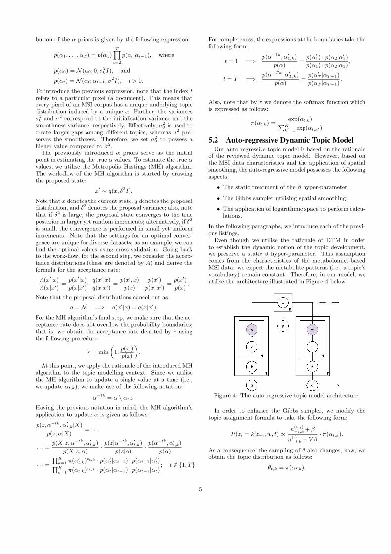
Even though we utilise the rationale of DTM in orderto establish the dynamic notion of the topic development,we preserve a static β hyper-parameter. This assumptioncomes from the characteristics of the metabolomics-basedMSI data: we expect the metabolite patterns (i.e., a topic’svocabulary) remain constant. Therefore, in our model, weutilise the architecture illustrated in Figure 4 below.

Figure 4: The auto-regressive topic model architecture.

In order to enhance the Gibbs sampler, we modify thetopic assignment formula to take the following form:

P (zi = k|z−i, w, t) ∝n(wi)−i,k + β

n(·)−i,k + V β

· π(αt,k).

As a consequence, the sampling of θ also changes; now, weobtain the topic distribution as follows:

θt,k = π(αt,k).

5

Finally, we address the computational stability by per-forming calculations in logarithmic space. Effectively, theapplication of logarithmic space mitigates the susceptibil-ity to numerical underflow. Note that numerical underflowis especially relevant in the context of probabilistic models:calculations involve large products of probabilities. In log-arithmic space, however, the products are transformed intosums. Relating to our model, we apply logarithmic space forboth the auto-regressive α update and the sampling-basedinference. The updated expression for the auto-regressive αupdate is given as follows:

log

[p(z, α−tk, α′

t,k|X)

p(z, α|X)

]= . . .

. . . = log[p(z, α−tk, α′

t,k|X)]− log

[p(z, α|X)

]. . . = zt

K∑k=1

log[π(α′

t,k)]+ log

[p(α′

t|αt−1)]+ log

[p(αt+1|α′

t)]

− zt

K∑k=1

log[π(αt,k)

]+ log

[p(αt|αt−1)

]+ log

[p(αt+1|αt)

].

As a result, the acceptance rate takes the following expres-sion:

rt,k = exp[min

(0, log

[p(z, α−tk, α′

t,k|X)]− log

[p(z, α|X)

])].

To introduce the updated expression for the inference, it isexpressed as follows:

P (zi = k|z−i, w, t) ∝ . . .

. . . ∝ log[n(wi)−i,k + β

]− log

[n(·)−i,k + V β

]+ log

[π(αt,k)

].

5.3 Data Pre-processing and Generative Pro-cess

In this subsection, we introduce the MSI data format usedin the experiments. At the start, we introduce an exampleof real data. Effectively, the example displays an applicationof the pre-processing techniques presented in the literaturereview section. Further, we transfer the qualities of realMSI data into our synthetic data generation module. Tobe more specific, we provide an algorithm for the generativedata process.

Before carrying the experiments, we familiarise with rawMSI data characteristics and assess their scalability. To bemore specific, we define the characteristics of our syntheticdata by pre-processing a real MSI data sample. To introducethe pre-processing details, we dismiss the words below theintensity threshold of 10; then, we apply the following buck-etisation strategy: merge adjacent vocabulary terms whichdiffer less than 7 mDa. Effectively, the bucketisation strat-egy is based on the spectral peak identification. Finally,we apply linear baseline scaling to align the highest inten-sities to 25. Most importantly, note that these settings areunique with every dataset; however, the provided values al-low carrying experiments in a scalable manner (i.e., a singleexperiment run on one dataset would take approximately 60minutes).

At this point, we take an exemplary sample. Note that,in the sample, there are two letters inscribed with the inkcorresponding to a particular mass-to-charge value. In Fig-ure 5, we compare the visualisation of the sample with andwithout the applied pre-processing.

(a) The ‘b and e’ term’s occurrences before linear baseline scaling.

(b) The ‘b and e’ term’s occurrences after linear baseline scaling.

(c) An inferred topic corresponding to the ‘b and e’ pattern.

Figure 5: The comparison of the ‘b and e’ term’s extraction.

Having the basis for a scalable inference, we transfer theidentified data properties into the synthetic corpus genera-tion. Before introducing the generative process, recall thatour dynamic topic treatment is unique with respect to ev-ery document. Therefore, contrary to the reviewed dynamictopic models, our dynamic segment consists of only one doc-ument. Considering the latter aspects, we establish ourutilised generative using Algorithm 1 given below:

Algorithm 1 The generative process for a synthetic corpus.

for t← 1, T do2: N ∼ Poisson(ξ)

for n← 1, N do4: zt,n ∼ Multinomial(π(αt))

k = {i : zt,n,i = 1}6: wt,n ∼ Multinomial(ϕk)

end for8: end for

In practical settings, the rationale of the generative pro-cess is defined as follows: the ξ term represents an approx-imate number of words per document; αt is the pre-definedauto-regressive hyper-parameter for the document t; and ϕk

is the pre-defined vocabulary term distribution for the topick.

6. EXPERIMENTSIn this section, we assess the research problems introduced

in Section 3:

• The spatial smoothing application for recovering theunderlying vocabulary term distributions;

• The auto-regressive model’s performance in terms ofidentifying the noise topic.

At the start of the section, we define the settings for tuningthe topic models; then, we look into the settings for gener-ating the synthetic datasets; afterwards, we introduce the

6

scope of our experiments. Having defined the settings, weprovide several illustrative examples of the experiment ex-ecution; and finally, we show the results of the performedexperiments.

6.1 Pre-experiment SettingsThe performance of the experiments is assessed by running

the auto-regressive and non-auto-regressive topic models inparallel. That is, we run the topic models with and withoutthe pre-set assumption of spatial smoothing. For both mod-els, we tune the variances corresponding to the α updateintroduced in Section 5. Recall that the variance δ2 is usedto propose a new α hyper-parameter’s state; the variance σ2

0

is used to initialise α0; and the variance σ2 controls spatialsmoothing. Effectively, in the non-auto-regressive model, wedo not have the σ2 term as all α terms are initialised usingσ20 (this notion relaxes the assumption of spatial smoothing).In order to run the experiments in an efficient manner, we

identify optimal values of the previously noted variances.One reason behind the variance tuning corresponds to therate of convergence upon the application of the MH algo-rithm. Based on the algorithm’s rationale – a low accep-tance rate indicates a slow and stable convergence, whereasa high acceptance rate indicates a random and unstable con-vergence – we would find the variance δ2 inducing the ac-ceptance rate of around 30%. Another reason behind thevariance tuning is related to the spatial smoothing applica-tion. Most importantly, we keep the variance σ2 in tact withthe rate of change of the topic smoothing throughout thedata. Furthermore, since the topic development is capturedin discrete space, we want to make sure that the discretisa-tion step induced by the generative data process is smallerthan the σ2 variance; otherwise, we would fail to capturethe high rate of change induced by steep topic changes.

To comment on the datasets generated for the experi-ments, these are designed to reflect the three following as-pects: the effect of overlapping topics; the effect of overlap-ping vocabulary terms; and the effect of noise. Note thatour assessment is based on an intuitive 3 topic scenario: 2topics model distinct metabolite entities, and the remainingtopic models the noise topic. To comment on the datasetsize, we set T = 50 for the number of documents per cor-pus and ξ = 100 for the number of words per documents:the choice of T surpasses the discretisation concern; also, assuggested by the generative algorithm given in Subsection5.3, the use of the ξ parameter establishes a slightly varyingnumber of words in each document. However, in order tospeed up the inference, we normalise the number of wordsper document to possess the maximum value of 50.

In the following figures, we illustrate the variations of thedata generation settings: in Figure 6, we display the settingcontrolling the topic overlap; in Figure 7, we display the set-ting controlling the topic term overlap; and in Figure 8, wedisplay the setting controlling the error overlap. Note thatthe red and green colourings indicate the synthetic metabo-lite topics; the green colouring indicates the noise topic; and,for the term names set in the horizontal axes of Figures 7and 8, we use arbitrary, unique numbers.

Relating the latter settings to our experiments, we assesstheir all (eight) possible permutations. To give an exam-ple of a permutation, one of the experiments would assessthe ability to recover the underlying topic term distribu-tions with the enabled topic overlap, the disabled topic term

Figure 6: Controlling the topic overlap.

Figure 7: Controlling the topic term overlap.

Figure 8: Controlling the error overlap.

7

overlap, and the enabled error overlap. Note that the lattersettings directly reflect the θ and ϕ values of the syntheticdatasets (we do not use the α and β hyper-parameters). Byfollowing the latter principle, we establish a clearer represen-tation of the synthetic data; thus, simplify the performanceassessment.

6.2 Experiment executionBefore going into the experiment execution, note that we

assess the performance based on the models’ ability to re-cover the underlying synthetic corpus generation settings.To wrap this assessment into a more concise terminology,the true solution corresponds to the underlying syntheticcorpus generation settings; and the approximate solutioncorresponds to the inference results. As a result, the per-formance is measured by taking the difference between thetrue and approximate solutions.

In order to introduce the rationale behind the perfor-mance assessment, we look into one of the eight experi-ments in more detail. Just like for all our experiments, werun both auto-regressive and non-auto-regressive models for5000 Gibbs sampling iterations, 1000 of which are dedicatedto the burn-in process. For each of the remaining 4000 iter-ations, we sample the corresponding θ and ϕ values; after-wards, in every 100th iteration, we average the stored θ andϕ values, respectively; then, this average is compared to thetrue solution. As an example, in the 1100th iteration, wewould take the average of 100 samples; in the 1200th itera-tion, we would take the average of 200 samples. In a singleexperiment, we would have 40 of such batches indicating theperformance – this is illustrated in Figure 9 and Figure 10.

Figure 9: The θ recovery performance.

Figure 10: The ϕ recovery performance.

Relating to the previous example, the θ and ϕ values cor-responding to the last iteration are illustrated in Figure 11and Figure 12, respectively. Also, note that we relax thecolour coding of our figures as the topics are inferred in un-supervised manner.

Figure 11: The comparison of the θ values.

Figure 12: The comparison of the ϕ values.

8

To assess the auto-regressive model’s performance, we havegenerated 10 distinct datasets for each previously introducedcorpus generation setting. Recall that we assess the fol-lowing conditions: the topic overlap; the vocabulary termoverlap; and the error term overlap. For every setting per-mutation, we perform the two-tailed t-test: the t-statisticsuggests the difference in performance; and the p-value sug-gests whether the result is significant. To be more specific, anegative t-statistic indicates the auto-regressive model’s su-perior performance; whereas the results are determined tobe significant if the p-value is below 0.05. The t-statisticsand p-values of all eight performed experiments are providedin Table 1 below.

Overlap t-statistic p-valueTopic Term Error θ ϕ θ ϕ

False True True −5.41 0.47 0.00 0.65False True False −9.46 −0.38 0.00 0.71False False True 4.74 3.93 0.00 0.00False False False −2.91 −3.24 0.02 0.01True True True −5.99 −1.71 0.00 0.12True True False −1.78 −1.53 0.11 0.16True False True 1.12 1.17 0.29 0.27True False False 0.52 1.10 0.61 0.30

Table 1: The t-test assessing 8 different overlap settings.

Based on the obtained results, the most significant changes(the p-values vary from 0.00 to 0.01) occur upon only switch-ing the error overlap setting (the remaining settings are dis-abled). If the error overlap is disabled, the spatial smooth-ing application displays an improved performance (i.e., 3.24lower error in recovering ϕ); however, if the setting is en-abled, the auto-regressive model performs poorly (i.e., 3.93higher error in recovering ϕ). Further, by relaxing the sig-nificance threshold, we can also consider the experiment in-stances where the p-values vary from 0.12 to 0.16. Conve-niently, in this experiment pair, we again consider only theswitch of the error overlap setting; however, in this case, allother settings are enabled. To comment on the respectiveperformance, the spatial smoothing application is superiorin both cases: 1.71 and 1.53 lower error rates in recoveringϕ.

Interestingly, we can group the experiment listings in fourpairs: the pairs are centred around the ϕ p-values of 0.01,0.16, 0.30, or 0.71. The first two pairs are presented in theprevious paragraph; however, for the last two pairs, the p-values are well beyond the significance threshold. By notingthat, in every pair, only the error setting varies, the insignif-icant results occur when one of the topic and term settingsis disabled and another is enabled. By looking into the ϕrecovery plots related to the insignificant results, we noticedthat both auto-regressive and non-auto-regressive models in-fer similar latent ϕ distributions. Effectively, in the case ofthe enabled error setting, both models simplify the datasetcomplexity; that is, the models assign the overlapping errorterms to the main topics. Alternatively, in the case whenthe error setting is disabled, the problem is too simple –both models recover the ϕ values equally well. To give anexample of a similar performance, the reader can considerthe previously introduced Figure 10 and Figure 12. How-ever, by examining Figure 10, note that the ϕ value of theauto-regressive model converges faster.

7. CONCLUSIONIn this research paper, we reviewed an attempt to induce

spatial smoothing in MSI data: the research problematic wassupported and inspired by covering the relevant literature;the model’s design was introduced by providing the prelim-inary knowledge covering LDA, spatial smoothing, and MSIdata pre-processing; finally, the experiment settings were de-signed to identify both superior and inferior spatial smooth-ing application prospects.

Our main objectives were to identify the spatial smooth-ing application’s prospect in recovering the ϕ values usedupon the generative data process and the ability to separatethe noise topic. We report that only a half of the carried ex-periments displayed a significant performance in recoveringthe ϕ values. To be more specific, we observe an improvedϕ recovery when the synthetic datasets are generated us-ing enabled topic and terms overlap settings; alternatively,when both topic and term overlap settings are disabled, theperformance is superior if the error overlap is disabled andinferior if the error overlap is enabled.

To expand on the overlapping noise topic’s identification(i.e. noise detection), the auto-regressive model – just likethe non-auto-regressive model – assigns the overlapping er-ror terms to the main topics. For this reason, we concludethat the spatial smoothing application is negligible in im-proving the overlapping noise topic term detection. How-ever, looking into the statistical test on the θ values, 6 out 8experiments display a significant performance in recoveringthe θ values. In 5 out 6 cases, the θ values are recovered witha lower error; this result is mostly impacted by the model’sability to reflect the shape of the noise topic with a betteraccuracy.

Since some of the experiment settings display a perfor-mance improvement, the spatial smoothing application couldbe considered for a further research. We would recommendlooking into the application of the undirected graphical model– Markov random field. Effectively, the application wouldestablish more complex spatial smoothing settings: the spa-tial treatment of neighbouring entities could be improvedfrom 1-dimensional to 2- or 3-dimensional. Effectively, thespatial dimensionality escalation would reflect the visual as-pect of MSI data better.

To suggest an alternative research direction in assessingthe spatial smoothing application, we propose a researchproblem on investigating bucketisation enhancements. Inother words, the spatial smoothing application might havean impact upon the feature extraction from MSI data. Tobe more specific, spatial smoothing might establish moreappropriate bucket size ranges in concatenating raw mass-to-charge values. If successful, this application would improvethe quality of MSI data features and, consequently, improvethe performance of the research problems addressed by thisresearch project.

To give the final verdict on the research project’s out-come, we consider the performance obtained using the set-tings reflecting the metabolomics environment the best. Ef-fectively, the more overlap settings are enabled, the betterthe metabolomics environment is represented. As shown byTable 1, the auto-regressive model tends to perform bet-ter when most of the overlap settings are enabled. There-fore, we conclude that spatial smoothing can be indeed ef-fective on improving the assessment of the MSI data withmetabolomics environment characteristics.

9

8. REFERENCES[1] A. Alonso, S. Marsal, and A. Julia. Analytical

methods in untargeted metabolomics: state of the artin 2015. Frontiers in bioengineering and biotechnology,3:23, 2015.

[2] D. M. Blei. Probabilistic topic models.Communications of the ACM, 55(4):77–84, 2012.

[3] D. M. Blei and J. D. Lafferty. Dynamic topic models.In Proceedings of the 23rd international conference onMachine learning, pages 113–120. ACM, 2006.

[4] D. M. Blei, A. Y. Ng, and M. I. Jordan. Latentdirichlet allocation. Journal of machine Learningresearch, 3(Jan):993–1022, 2003.

[5] B. M. Bolstad, R. A. Irizarry, M. Astrand, and T. P.Speed. A comparison of normalization methods forhigh density oligonucleotide array data based onvariance and bias. Bioinformatics, 19(2):185–193,2003.

[6] A. Craig, O. Cloarec, E. Holmes, J. K. Nicholson, andJ. C. Lindon. Scaling and normalization effects in nmrspectroscopic metabonomic data sets. Analyticalchemistry, 78(7):2262–2267, 2006.

[7] T. De Meyer, D. Sinnaeve, B. Van Gasse,E. Tsiporkova, E. R. Rietzschel, M. L. De Buyzere,T. C. Gillebert, S. Bekaert, J. C. Martins, andW. Van Criekinge. Nmr-based characterization ofmetabolic alterations in hypertension using an

adaptive, intelligent binning algorithm. AnalyticalChemistry, 80(10):3783–3790, 2008.

[8] L. Du, W. Buntine, H. Jin, and C. Chen. Sequentiallatent dirichlet allocation. Knowledge and informationsystems, 31(3):475–503, 2012.

[9] T. L. Griffiths and M. Steyvers. Finding scientif ictopics. Proceedings of the National academy ofSciences, 101(suppl 1):5228–5235, 2004.

[10] S. M. Kohl, M. S. Klein, J. Hochrein, P. J. Oefner,R. Spang, and W. Gronwald. State-of-the art datanormalization methods improve nmr-basedmetabolomic analysis. Metabolomics, 8(1):146–160,2012.

[11] A. Palmer, P. Phapale, I. Chernyavsky, R. Lavigne,D. Fay, A. Tarasov, V. Kovalev, J. Fuchser,S. Nikolenko, C. Pineau, et al. Fdr-controlledmetabolite annotation for high-resolution imagingmass spectrometry. Nature Methods, 2016.

[12] R. Smith, A. D. Mathis, D. Ventura, and J. T. Prince.Proteomics, lipidomics, metabolomics: a massspectrometry tutorial from a computer scientist’spoint of view. BMC bioinformatics, 15(7):S9, 2014.

[13] J. J. J. van der Hooft, J. Wandy, M. P. Barrett, K. E.Burgess, and S. Rogers. Topic modeling for untargetedsubstructure exploration in metabolomics. Proceedingsof the National Academy of Sciences, page 201608041,

2016.

10