Spatial Disparities in Developing Countries: Cities...
39
Spatial Disparities in Developing Countries: Cities, Regions and International Trade Anthony J. Venables November 2003
Transcript of Spatial Disparities in Developing Countries: Cities...

Spatial Disparities in Developing Countries: Cities,
Regions and International Trade
Anthony J. Venables
November 2003

Abstract Spatial inequality in developing countries is due to the natural advantages of some regions relative to others and to the presence of agglomeration forces, leading to clustering of activity. This paper reviews and develops some simple models that capture these first and second nature economic geographies. The presence of increasing returns to scale in cities leads to urban structures that are not optimally sized. This depresses the return to job creation, possibly retarding development. Looking at the wider regional structure, development can be associated with large shifts in the location of activity as industry goes from being inward looking to being export oriented. Key Words: cities, spatial disparities, urbanisation, developing countries. JEL classification: R1, R12, O18 This paper was produced as part of the Centre’s Globalisation Programme The Centre for Economic Performance is financed by the Economic and Social Research Council Acknowledgements This paper was produced as part of the UNU-WIDER project on Spatial inequalities in developing countries. Professor Venables is Director of the Globalisation Programme at the Centre for Economic Performance and Professor of International Economics, London School of Economics and Political Science. He is also a Research Fellow at the Centre for Economic Policy Research. Contact details: A.J. Venables, London School of Economics, Houghton Street, London WC2A 2AE, UK. Email: [email protected]; Web information: http://econ.lse.ac.uk/staff/ajv/ Published by Centre for Economic Performance London School of Economics and Political Science Houghton Street London WC2A 2AE All rights reserved. No part of this publication may be reproduced, stored in a retrieval system or transmitted in any form or by any means without the prior permission in writing of the publisher nor be issued to the public or circulated in any form other than that in which it is published. Requests for permission to reproduce any article or part of the Working Paper should be sent to the editor at the above address. A. J. Venables, submitted 2003 ISBN 0 7530 1671 0 Individual copy price: £5

1
1. Introduction
There are now numerous studies charting the evolution of spatial disparities during economic
development. In many countries a subset of regions leads in manufacturing activity, creating
jobs and drawing in population from other regions. This can be seen most clearly in the
experience of some of the large developing countries, such as China, Mexico, Brazil and
India but also occurs in smaller countries. In Mexico manufacturing has become highly
concentrated in regions that border the US, and spatial variation in per capita incomes has
increased dramatically since the mid 1980s (Cikurel 2002). In China, Demurger et al (2002)
chart increasing spatial inequalities in per capita GDP from the mid 1980s: coastal provinces
experienced the greatest decline in the share of agriculture in employment and output, and the
fastest growth of per capita income. In India, southern states have come to prominence in
manufacturing and tradable services (Besley and Burgess 2002).
The spatial concentration of new activities also occurs at a much finer level of
disaggregation than suggested by state or province level data. In virtually all countries
development is associated with urbanisation and the growth of prime cities, often far more
dominant in modern developing countries than are (or were) such cities in the developed
world. The number of cities in the world with a population of more than 1 million went from
115 in 1960 to 416 in 2000; for cities of more than 4 million the increase was from 18 to 53,
and for more than 12 million from 1 to 11 (Henderson and Wang 2003). In some cases the
most successful cities exhibit a high degree of sectoral specialisation -- for example,
Bangalore’s software specialism. The growth of cities tells us that, despite diseconomies
associated with developing country mega-cities, there are even more powerful economies of
scale making it worthwhile for firms to continue to locate in these cities.

2
These changes in spatial structure indicate a ‘lumpiness’ in economic development.
Far from being a process of smooth convergence, development is highly spatially
differentiated. This poses a number of questions for economic theory. The first is, why do
these spatial disparities develop? This question can be addressed by drawing on the
economic geographer’s distinction between first nature and second nature geography. First
nature simply says that some regions are favoured by virtue of endowments or proximity to
rivers, coasts, ports and borders. Evidently, these factors account for much of the success of
coastal China relative to the north-west, or border states of Mexico relative to the south.
Second nature emphasises the interactions between economic agents, and in particular the
increasing returns to scale that can be created by dense interactions. Thus, cities tend to have
high productivity, and agglomeration forces act to generate virtuous circles of self-
reinforcing development. These forces have been extensively researched in recent years
although much remains to be done, particularly in the context of developing countries.1 What
determines the strength of these forces? How do they depend on aspects of the economic
environment such as openness to trade, the stock of labour skills, and the policy
environment?
The second question is: how do spatial disparities evolve during development, and to
what are extent are they self-correcting or persistent? Empirically, we know from the work
of Williamson (1965) and others that there is a tendency for spatial inequalities to increase
and then decrease. But from the standpoint of theory, what factors are conducive to spread of
activity or to persistence of disparities? Is there a ‘normal’ pattern that countries might be
expected to follow? As development proceeds to what extent does activity spread out of
existing agglomerations, and to what extent is labour drawn into these centres? These
questions are particularly important in the context of urbanisation. The development of new

3
urban centres likely involves increasing returns, arising from both infrastructure investments
and clustering externalities between firms. How easy is it for new centres of activity to
become established, or does activity tend to be locked in to existing centres? What
institutional structures are conducive to the birth of new centres and the consequent spread of
activity?
The third set of questions are to do with real income and welfare, in both the short-
and the long-run. Second nature agglomeration forces are inherently associated with market
failure so equilibrium city structures are likely to be inefficient. Are developing county cities
too large or too small, and are there too many or too few of them? Should new city
development be promoted or neglected? Most importantly, just as growth shapes the spatial
structure of the economy, so also the spatial structure shapes the growth process. If a
country’s spatial structures are wrong then this may reduce the returns to modern sector
investment and thereby damage long run growth.
This paper takes some steps towards addressing these issues, investigating the spatial
path that a growth process might take and the welfare properties of this path. We first
(section 2) draw on standard models of urban economics, extending these models to
incorporate both first and second nature geography, and using them to investigate the
consequences of alternative urban institutional structures. We show that market failures lead
to sub-optimal city size structures and, by depressing the return to job creation, can retard
development and perhaps also create the possibility of being stuck in a low level equilibrium
trap. We then (section 3) move on to the broader picture of regional development. Whereas
in the urban models all spatial linkages are within cities, in this section we draw on ‘new
economic geography’ models to capture broader spatial interactions. These models illustrate

4
how there can be dramatic shifts in countries’ internal economic geography during the
process of development.
2. Cities
We start by setting out a simply analytical framork within which the relationship between
city structure and economic growth can be examined. We suppose that, in a given country,
there are a large number of potential city locations, labeled by subscript i. These are not all
‘greenfield’ and may include existing towns or cities which are potential hosts for the
development of modern sector activity.2 The number of workers in such sectors in city i is ni.
These can be thought of as ‘worker-firms’, whose productivity in city i is given by qia(ni) so
the total output of the city is niqia(ni). This productivity function has two components. The
first, qi, captures the ‘first nature’ characteristics of the city. These include city ‘endowments’
– such as location, climate, and business environment -- and also spatial variations in prices.
For example, one way to think of qi is in terms of cities producing an export good, the price
of which (net of trade costs) depends on distance from a coast or border. We order cities such
that i = 1 is the best location and qi is decreasing with i.
The second component, a(ni), captures the idea that productivity depends on the
number of workers in the same city, ni. We generally take a(ni) to be increasing, at least up to
some point, and concave. Thus there are initially increasing returns to expanding each city,
although beyond some point negative externalities may come to dominate so further increases
in city size reduce productivity. Importantly, these returns to scale operate at the city level, so
are external to the actions of individual worker-firms. Whenever a’(n) … 0 externalities are
present, creating market failure, unless some institution exists to internalise them. The source
of the returns to scale may be knowledge spillovers or thick market effects, but in this section

5
(1)
of the paper we will not model the underlying forces driving these returns to scale, simply
taking their presence as a fact.3
Scarcity of land in each location means that land prices are increasing with
population. Drawing on the urban economics tradition to model this, city workers pay a
commuting cost, (linear in distance) to reach the central business district in each city. We
assume that cities occupy a linear space and each worker occupies one unit of land.4 If
commuting costs are 2t per unit distance, then a city with n workers has total commuting
costs of , creates rents of , and has rent plus commuting costs per worker of .
In addition to its cities, each economy has an agricultural sector producing output
where L is the economy’s total labour force, and N is total urban employment,
. The production function Y(.) is strictly concave, so an increase in the total urban
population, N, raises the marginal product and the wage in agriculture, , w’
> 0. The economy is open to trade and faces constant world prices for its output. For
simplicity we assume that consumer goods (apart from land) have the same price (unity) in
all locations. Housing and agricultural rents are distributed equally amongst the population in
a lump sum manner.
The private return to a job in city i will be denoted B(ni , qi ) and takes the form
This is the value of output generated by the job, minus the costs of employment. These are
the agricultural wage, w(N), and the commuting cost plus rent of workers (equal to the
commuting costs of the marginal worker). Our key assumption is that B(ni , qi ) is increasing
in ni up to some value, diminishing thereafter, and concave. This arises as increasing returns
in the technology, a’ > 0, are offset by commuting costs, t; at low values of employment qi a’

6
> t, but concavity of a(ni) means that beyond some point this inequality is reversed. We also
assume that at low values of N there are spatial distributions of ni for which some Bi are
strictly positive – ie, the technology qia(ni) is good enough for this economy to be able to
develop an urban structure.
2.1 First nature, second nature and urban growth
The framework we have set out incorporates both first and second nature geography. What do
these forces imply for the spatial pattern of growth and development? Before turning to a
detailed analysis of the determinants of city structure we motivate the discussion by
illustrating some possible development paths.
As outlined above, locations are ranked according to productivity parameter qi.
Suppose first that there are no increasing returns or externalities, so a’(n) = 0 for all n. With
this assumption B(ni , qi ) is decreasing in ni What does growth look like in this economy?
Figure 1a gives an illustrative example. The horizontal axis is N, the total employment in
manufacturing, and we assume that this increases at a rate that is exogenously given. (We
return to fuller treatment of this in sections 2.3 and 2.4). The vertical axis is employment in
each location, and the curves give employment for the best location, n1, second best, n2 and
so on. Worker-firms are perfectly mobile, and go wherever the returns to a job are highest.
Equilibrium ni is therefore determined by the condition that all active cities have the same
value of B(ni , qi ), a value which exceeds that in any location that is not active.5 The growth
pattern is as would be expected. At any point in time (any value of N) only a subset of
potential locations are active, this determined by their first nature advantage. Increasing N
causes both intensive and extensive growth. Existing cities get larger but they encounter
diminishing returns to scale because of the presence of commuting costs. This reduces the

7
returns to a job in the city, B(ni , qi ), making it worthwhile to start activity in the next city,
and so on.
Evidently, this economy has a spatial structure that evolves during development, and
there is increasing then decreasing spatial disparity as activity is initially concentrated in a
few locations, then spreads out. The spatial structure described is a distribution of
employment, but what about the distribution of income? Urban workers receive a nominal
income greater than the agricultural wage in order to cover their rent and commuting costs,
and, given a value of N, there may also be surplus earned on each urban job, B(ni , qi ) > 0.
Whether urban workers have higher real income than agricultural depends on the distribution
of this surplus between workers and firms, which may in turn depend on local labour market
conditions and the willingness of workers to migrate. We investigate these issues no further
in the present paper, but see Kanbur and Rappoport 2003.
How are things different when second nature geography is also present? A non-
convexity arises because B(ni , qi ) is increasing in employment for small values ni, before it
starts decreasing. The incentive to start a new city now depends on the mass of workers who
can coordinate their decisions. We discuss this in more detail in section 2.2 below, and now
simply assume that active cities expand up to the point at which it becomes profitable for a
single small worker-firm to set up in a new location. Thus, employment levels are such that
each active city has the same return to jobs, B(ni , qi ). Expansion eventually brings a decline
in this return, and a new city is born when it reaches the level at which it equals the return to
establishing a job in a new location. An illustration of the associated growth process is given
in figure 1b.
The growth process is now much ‘lumpier’, with cities developing in sequence, rather
than in parallel. First nature determines the order of development and, at any point in time,
8
predicts which locations are successful and which are not. However, the dependence of
performance on first nature is not continuous. Very small differences in first nature can
translate into large differences in outcomes for locations at the margin of development.
Conversely, improving a location’s first nature does not necessarily confer any immediate
payoff in terms of attracting the activity, as the location may remain below the current
threshold. And amongst the set of active locations, differences in first nature have little effect
on employment, as they are dominated by acquired second nature advantages. Furthermore,
development is more spatially concentrated with (for any given value of N) activity
concentrated in fewer and larger locations. This is consistent with the stylised facts as we
outlined them in the introduction. We should also note that it is likely that at least some of
increasing returns are sector, as well as location specific. Growth is then associated with the
development of sectorally specialised cities, and this too is consistent with evidence. Since
productivity functions are in this case sector specific, quite different city size structures might
be observed (Henderson 1974).
With this overview of the model we now turn to more detailed analysis. We first
(section 2.2) ask the question; what determines the size and number of cities, and what
inefficiencies are present at equilibrium? The answer to this question is sensitive to the
cities’ institutional structure -- the land market and the extent to which agents are able to
internalise the externality. This issue has been addressed in the literature (see Abdel-Rahman
and Anas 2003 for a survey). We argue that some of the institutional assumptions employed
in this literature are inappropriate, particularly for developing countries, and present some
new results. We then turn to a second question (section 2.3); how does urban structure affect
the incentive to create jobs and hence levels of modern sector employment, N? Different
institutional structures imply different values of job creation, B, so if N responds

9
(2)
(3)
endogenously to B, they will also imply different levels of modern sector employment and
wages. While section 2.3 gives a long run analysis, section 2.4 sketches a dynamic version of
the model, in which the market failures associated with urban development can lead to
multiple equilibria and the possibility of an economy being stuck in a low level equilibrium.
2.2 Optimal and equilibrium urban structures
Given the overall level of modern sector employment, N, are equilibrium city sizes larger or
smaller than socially optimal? The answer to this question depends on the extent to which
externalities are internalised, and we compare three different possibilities. The benchmark
case is the socially efficient outcome. For simplicity, we abstract from first nature for the
remainder of this section, making all locations ex ante identical (qi = q) and dropping the
subscript i. To find the socially optimal outcome we maximise the following expression,
in which there are k active cities each with population n. The first term is the value of output
minus resources used in commuting in these k cities, and the second is the value of output in
the agricultural sector. The last term captures the fact that total urban employment is fixed at
N, so 8 is the lagrange multiplier on the constraint that nk should not exceed N. Ignoring
integer constraints, the first order conditions for welfare maximisation with respect to the size
of each city, n, and the number of cities, k, are,
and
10
(4)
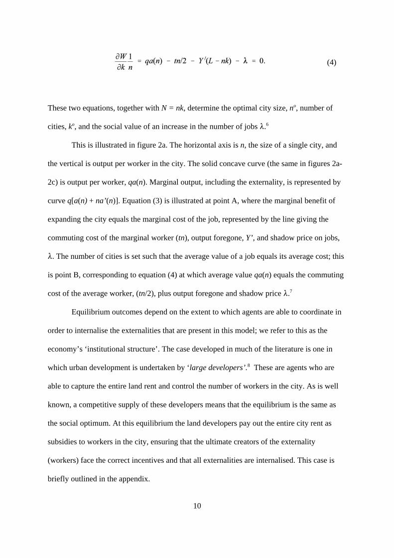
These two equations, together with N = nk, determine the optimal city size, no, number of
cities, ko, and the social value of an increase in the number of jobs 8.6
This is illustrated in figure 2a. The horizontal axis is n, the size of a single city, and
the vertical is output per worker in the city. The solid concave curve (the same in figures 2a-
2c) is output per worker, qa(n). Marginal output, including the externality, is represented by
curve q[a(n) + na’(n)]. Equation (3) is illustrated at point A, where the marginal benefit of
expanding the city equals the marginal cost of the job, represented by the line giving the
commuting cost of the marginal worker (tn), output foregone, Y’, and shadow price on jobs,
8. The number of cities is set such that the average value of a job equals its average cost; this
is point B, corresponding to equation (4) at which average value qa(n) equals the commuting
cost of the average worker, (tn/2), plus output foregone and shadow price 8.7
Equilibrium outcomes depend on the extent to which agents are able to coordinate in
order to internalise the externalities that are present in this model; we refer to this as the
economy’s ‘institutional structure’. The case developed in much of the literature is one in
which urban development is undertaken by ‘large developers’.8 These are agents who are
able to capture the entire land rent and control the number of workers in the city. As is well
known, a competitive supply of these developers means that the equilibrium is the same as
the social optimum. At this equilibrium the land developers pay out the entire city rent as
subsidies to workers in the city, ensuring that the ultimate creators of the externality
(workers) face the correct incentives and that all externalities are internalised. This case is
briefly outlined in the appendix.
11
(5)
(6)
(7)
Despite the widespread use of this as a modelling approach, it seems hard to imagine
that the large developer case is an appropriate description of land markets and city growth in
developing countries, requiring, as it does, that a single developer controls city employment
by subsidising the optimal number of workers to enter. We therefore investigate two
alternatives to the large developer model. In both of these we assume that location decisions
are taken by worker-firms who are not also landowners, so do not capture all the rent
associated with urban development. The two cases differ however, in the extent to which the
worker-firms can coordinate their decisions, so internalising reciprocal externalities in
production.
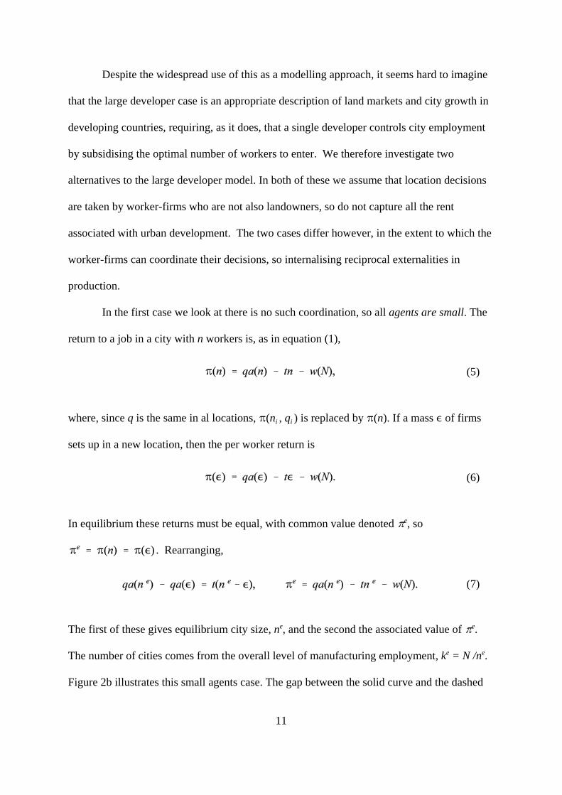
In the first case we look at there is no such coordination, so all agents are small. The
return to a job in a city with n workers is, as in equation (1),
where, since q is the same in al locations, B(ni , qi ) is replaced by B(n). If a mass , of firms
sets up in a new location, then the per worker return is
In equilibrium these returns must be equal, with common value denoted Be, so
. Rearranging,
The first of these gives equilibrium city size, ne, and the second the associated value of Be.
The number of cities comes from the overall level of manufacturing employment, ke = N /ne.
Figure 2b illustrates this small agents case. The gap between the solid curve and the dashed

12
(8)
line is the per worker return, and this equals the common value Be
at points A and B, respectively a city of size ne and a city of size , = 0. Thus, cities expand
upto size ne, beyond which it is profitable to start a new city.
If all agents are small, then , = 0 in the equations above. However, a further
possibility is that a coalition of producers is able to coordinate decisions to start production
in the city, although not able to capture the land rents that are generated by city growth. If a
producer coalition of any size , can form a new city then it will do so if B(,) is greater than
or equal to the return in an established location, B(n). We denote argmax B(,) / nc, and from
inspection of (6) see that the first order condition is The equilibrium city size
and returns to a job are therefore,
To understand this case consider first the vertical line nc on figure 2b. Entry at this scale
would clearly yield returns per job greater than Be. Coalitions are able to exploit this, in a
way that small agents cannot, and bid away this area of surplus. The outcome is as illustrated
in figure 2c, with equilibrium size nc and profit level Bc. This is the highest attainable level
of B by producers faced with given w(N) and for whom the whole of commuting costs plus
rent (tn) is a cost.
Comparison of equilibrium and optimum city size
Two market failures are present, creating the differences between cases. The first is the
externality in production as each worker-firm affects the productivity of all others; since this
is a reciprocal externality it generates a potential coordination failure amongst worker-firms.
The second arises as surplus is divided between worker-firms and landlords; this internal

13
(9)
‘terms of trade’ means that agents do not necessarily receive the full marginal benefit of their
actions.
These failures can be seen by looking at the size of cities when there is a coalition of
producers. It is unambiguously the case that nc < ne (see figures 2b and 2c). The producer
coalition overcomes the coordination failure, making it easier to establish new cities and
hence causing cities to be smaller than in the small agent case. It is also unambiguously the
case that nc < no. Comparing the tangencies at B and C on figures 2a and 2c respectively, the
value of extra output per worker, qa’(n), is equated to the increase in commuting costs plus
rent, t, in the case of the producer coalition, and to the increase in commuting costs, t/2, in the
case of the optimum (this being achieved by subsidising employment if the optimum is
decentralised by large developers). Intuitively, the producer coalition fails to capture the
additional land rent created by city enlargement, so cities are smaller than optimal.
Both market failures come into play in the comparison of the social optimum and the
small agents case. Small agents are not fully rewarded for city enlargement, but also find it
difficult to start a new city. Consequently, the comparison of ne with no is ambiguous. Some
light can be shed by looking at the case where the productivity function is quadratic, given by
Equations (3) – (8) then imply
Comparing the optimum with the small agents case, we see that if $q > 3t/2 then ne > no, the
case illustrated in the figures. In this case large production externalities, $, relative to
commuting costs, t, mean that the coordination failure is large relative to land rents. The

14
large coordination failure gives rise to larger and fewer cities than is socially optimal.
However, if the inequality is reversed then small agents may give rise to a structure with too
many and too small cities.9
2.3 Urbanisation and the rate of development
We saw in the preceding subsection that equilibrium and optimal outcomes differ in the size
and number of cities they support, given the total number of urban jobs, N. They also differ in
the value of job creation, (8 and B). Hence, in a long run equilibrium in which N is a function
of the value of a job, they will differ in the level of urban employment, N, and the wage w(N).
Figures 2a-2c give all the information we need to analyse the value of job creation and hence
compare the effects of different institutional structures on long run modern sector
employment.
The vertical intercepts marked on figures 2 give the wage plus the value (social, 8, or
private, B) of an urban job. Suppose that such a job can be created at constant cost, which can
be set at zero. In the ‘long run’ it will therefore be the case that 8 = Be = Bc = 0, as the
number of jobs is unconstrained and any rent associated with a job is bid down to zero. The
height of the intercept then just measures the equilibrium wage in the economy, Y’(L - N) =
w(N), and hence also indicates the magnitude of total urban employment.
The ranking is unambiguous and, as indicated on figures 2, takes the form w(No) >
w(Nc) > w(Ne ) and hence No > Nc > Ne . The first of these, No > Nc, comes from comparison
of figures 2a and 2c. In each of these figures optimising behaviour gives a tangency between
the marginal productivity gain and the marginal cost of expanding a city. In the case of
coordinated producers marginal commuting cost and rent is perceived as a cost of city
expansion, whereas in the optimum (and the case of large developers) marginal rent nets out.

15
(10)
This increases the return to establishing a city, and hence the return to urban employment.
The ranking of the coordinated producers and small agents cases is also unambiguous, with
Nc > Ne. This is a direct consequence of the fact that returns to job creation is optimised in the
first of these cases, but not in the second. With small agents there is an economic surplus that
is not being exploited, because of coordination failure, and this reduces the value of job
creation.
The implication of these findings are that different institutions affect not only city
sizes, but also the value of creating urban jobs. Failure to internalise the externalities
associated with urban development reduces the returns to job creation, so – depending on the
mechanism determining N – retarding development and lowering the wage.
2.4 Irreversible decisions and forward looking behaviour
So far we have assumed that decisions are made on the basis of instantaneous returns, as will
be the case if all decisions are costlessly reversible. We now briefly explore the polar
opposite case, in which a worker-firm commits to a location in perpetuity.
The number of workers active in a particular city, i, at date z we denote ni(z). The
instantaneous returns to a job in this city are,
where, for simplicity, we now assume that the wage is constant. Worker-firms are created at
constant rate of < per unit time. Consider a new city born at date 0; it receives workers at rate
< until some (endogenously determined) date T, at which point workers instead start to enter
the next city. The time path of returns to jobs in the city is given in figure 3. It rises and then
16
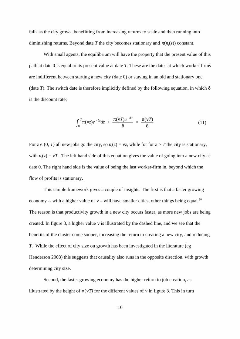
(11)
falls as the city grows, benefitting from increasing returns to scale and then running into
diminishing returns. Beyond date T the city becomes stationary and B(ni(z)) constant.
With small agents, the equilibrium will have the property that the present value of this
path at date 0 is equal to its present value at date T. These are the dates at which worker-firms
are indifferent between starting a new city (date 0) or staying in an old and stationary one
(date T). The switch date is therefore implicitly defined by the following equation, in which *
is the discount rate;
For z , (0, T) all new jobs go the city, so ni(z) = <z, while for for z > T the city is stationary,
with ni(z) = <T. The left hand side of this equation gives the value of going into a new city at
date 0. The right hand side is the value of being the last worker-firm in, beyond which the
flow of profits is stationary.
This simple framework gives a couple of insights. The first is that a faster growing
economy -- with a higher value of < – will have smaller cities, other things being equal.10
The reason is that productivity growth in a new city occurs faster, as more new jobs are being
created. In figure 3, a higher value < is illustrated by the dashed line, and we see that the
benefits of the cluster come sooner, increasing the return to creating a new city, and reducing
T. While the effect of city size on growth has been investigated in the literature (eg
Henderson 2003) this suggests that causality also runs in the opposite direction, with growth
determining city size.
Second, the faster growing economy has the higher return to job creation, as
illustrated by the height of B(<T) for the different values of < in figure 3. This in turn

17
suggests that, if the rate of job creation is an increasing function of the returns to creating a
job, so < = <(B), <’ > 0, then there may be multiple equilibria. In a slow growing economy it
is relatively difficult to start new cities; this reduces the return to job creation, B, reducing <,
and confirming the slow growth of the economy. Conversely, fast growing economies can
develop an urban structure that offers higher returns to job creation, confirming the rapid
growth of the economy.
3. Regions (and International Trade)
The models developed above imply that development is spatially concentrated, but the real
geographical structure of the models is rather weak, essentially because all the linkages
happen within cities. The only interaction between these locations is through markets which
are perfectly competitive and perfectly frictionless. To get a richer story of regional
disparities interactions between as well as within cities need to be added. One approach to
this is to work with a class of models in which the agglomeration force is transport costs on
goods which are produced subject to increasing returns to scale (internal to the firm).
Increasing returns means that a particular variety of good will typically only be produced in a
single place, and transport costs mean that there are gains to producing close to large
markets. Agglomeration can arise if there is labour mobility (so a large market creates jobs
and the expenditure of these workers makes the market large, Krugman 1991) or input-output
linkages, so firms create the market for other firms, (Venables 1996).
A model of this is sketched in the appendix (it draws on Fujita et al 1999), and we do
not elaborate it in the text. However, the key to understanding the forces operating in this
framework can be understood by looking at the wage equation – the maximum wage that a
firm can afford to pay in location i and break even. This wage, wi, is implicitly defined by

18
(12)
(13)
where Gi is a price index at location i, defined as
The right hand side of (12) is the ‘market access’ of location i, and is a theoretically well
founded version of market potential. It is the sum of expenditures, Ej, in all locations,
weighted by a trade cost factor and deflated by a price index. The trade cost factor, Tij, is a
measure of the cost faced by country i producers in selling in market j. The cost of living
index, Gi is defined in (13) as a CES aggregator (with elasticity of substitution F) of the
prices pi (trade cost adjusted) of each of the ni varieties of goods produced in each location.
Cross country variation in Gi arises as countries close to large sources of supply have lower
value of the price index.
The left hand side of (12) is the unit costs of a representative firm at location i. " and
$ are input shares, so if labour is the only input to production " = 0 and $ = 1. If
intermediates are used then " > 0 measures their share, and the price of a representative
bundle of intermediates is measured by the price index. This price index can also be
interpreted as the ‘supplier access’ of location i, taking a low value at locations that are close
to sources of supply of manufactured intermediates.
Pulling this together, we see that the maximum wage that a firm can afford to pay and
break even is greater the better its market access – the closer it is to sources of demand – and
the better its supplier access – lower G meaning cheaper inputs. This is a force for spatial

19
clustering of activity, and pulling against this is some dispersion force, such as land rents.
What light can this framework shed on spatial inequalities in developing countries?
3.1 2 region models
Puga (1998), using a framework similar to that outlined above, considered two regions in a
closed economy. He showed that if transport costs are high, there must be a ‘balanced’ urban
system, with a city in each region. The intuition comes from thinking of regional autarky, in
which each region has to produce all goods to meet local demand. However, at lower
transport costs consumer demands can be met by imports, so agglomeration forces give rise
to a primate-city structure. Manufacturing employment concentrates in a single city, which is
able to pay high wages because of its good market access (high value of the right-hand side
of (12)). Puga argues that this is one of the reasons why developing countries – urbanising
later and with better transport technologies – have a less balanced urban structure than do
present developed countries.
Working in a similar framework, Krugman and Livas (1996) show how openness to
international trade makes a more balanced city structure more likely. The intuition is that in a
more open economy firms are less dependent on local markets and local sources of supply, so
within city agglomeration forces are weaker. Given the presence of some dispersion forces,
trade can lead to a deconcentration of activity.
3.2 A multi-region model
Further insights can be gained by moving to a multi-region environment. A full version of
such a model could be calibrated to a particular country in order to show how the incentives
to locate in different regions evolves. Here we continue to operate with something more

20
stylised, and analyse a linear economy with a well defined mid-point and two end-points. In
line with the modeling of section 2, we continue to assume an exogenous growth process;
with the total number of manufacturing jobs, N, increasing through time. Where, in such an
economy, do they locate?
Industrialisation under autarky: We use numerical methods to explore equilibria of this
model, and present results in a series of contour plots.11 In figure 4a and subsequent figures
the vertical axis represents locations in the economy; thus, the top and bottom of the vertical
axis are the two ends of the linear economy. The horizontal axis is the share of the labour
force that is in manufacturing (N), varying from 1% to 30%. The contour lines on the figures
give manufacturing activity levels in each location.
Each point on the horizontal axis corresponds to an exogenously given number of
manufacturing firms in the country as a whole, and the model computes the equilibrium
location of these firms. Models of this type typically exhibit path dependence, so the process
by which more firms are added to the economy needs to be specified. In the results shown we
compute an initial equilibrium (at the left hand end of each figure). New firms are then
added to all locations, on top of the previous equilibrium pattern. Firms may relocate to the
most profitable locations, giving the new equilibrium. The process is repeated, moving to the
right along the figure.
The closed economy is illustrated in figure 4a. At low levels of manufacturing
development there are two manufacturing regions, located approximately 1/3 and 2/3 of the
way along the length of the economy. This locational pattern exhibits clustering, because of
the demand and cost linkages in the model. However, working against clustering is the
presence of demand for manufactures in all locations. The distribution of land across

21
locations means that income and expenditure on manufactures occurs everywhere, and
complete agglomeration of manufacturing in a single central cluster would leave
opportunities to profit from entry in peripheral regions. At low levels of overall
manufacturing activity the tension between the agglomeration and dispersion forces produces
an outcome with two distinct manufacturing regions.
As the economy becomes more developed, so we see that the two manufacturing
region structure breaks down and a single region forms, making the spatial distribution of
activity more concentrated. Why does this happen? The two region structure becomes
unstable because as the economy becomes more industrialised so agglomeration forces
become stronger. In particular, as manufacturing grows relative to agriculture the proportion
of demand for manufactures coming from the industrial regions becomes greater. This is a
force for moving the industrial centres inwards and away from the edges of the economy.
However, because of the lock-in effect created by agglomeration, this does not happen
smoothly. Instead, the two-centre structure remains an equilibrium up to some point at which
there is a bifurcation in the system, and a new structure develops, with a single central
industrial region. Further growth of manufacturing increases the number of firms in this
region and also (because of the diseconomies to city size that are present in the model) causes
some spread of the region to either side of the central location. What we see then, is the
closed economy developing a monocentric structure, with a large central manufacturing
region.
Industrialisation with two ports. How do things differ in a more open economy? Suppose
that the geography of the economy remains symmetric, with one port at each end of the
country. Outcomes are illustrated in figure 4b.
22
At low levels of industrialisation, there is now a single industrial region, located in
the centre of the economy. The reason is the presence of foreign competition, making
peripheral locations unprofitable. Firms derive natural protection from locating in the centre
of the economy. As the number of firms increases, so two things happen. First, central
regions of the economy become increasing well supplied with manufactures, driving down
their prices. And second, cost linkages strengthen, reducing costs and making manufacturing
better able to compete with rest of the world production. Both of these forces encourage a
dispersion of activity from the central region towards the edges of the economy. Once again,
there is a bifurcation point, but now the single cluster of activity divides into two clusters
closer to the ports. Despite the lock-in forces due to agglomeration, these centres exhibit
some movement towards the edge of the economy, becoming more dependent on export
markets as a destination for the growing volume of output. At some point the clusters reach
and concentrate at the port locations.
The broad picture is therefore one in which industrial development in the open
economy is associated with transition from a small centrally located and inwards oriented
manufacturing sector to its replacement by large export oriented clusters at the ports -- the
opposite of the autarky case. Two qualifications need to be made to this. If the domestic
economy were made a good deal larger, then the central cluster devoted largely to supplying
the domestic market could also survive, giving three manufacturing regions. And if returns
to clustering were made stronger then it is possible that manufacturing would agglomerate at
a single port. The gains to agglomeration at just one of the ports would outweigh any
diseconomies due to congestion or costs of supplying domestic consumers on the other side
of the economy.

23
Industrialisation with a single port. Finally we look at a case where geography is such that
trade can occur only through one end of the economy – a port located at the bottom edge of
figure 4c.
Like the previous case, at low levels of industrialisation there is a single industrial
cluster. This is now located more than half the length of the economy away from the port, in
order to benefit from the natural protection of distance. Industrialisation makes industry more
outward oriented and causes movement of this cluster towards the port. This movement
means that interior regions of the economy become progressively less well served by
manufacturing industry, and the economy reaches a bifurcation point at which a new spatial
structure emerges. A new industrial cluster forms in the interior of the economy, oriented
towards meeting local demands, and the original cluster is replaced by a cluster of
manufacturing in the port city. There is therefore a radical change in internal economic
geography, with the original monocentric structure being replaced by two industrial clusters,
one export oriented and the other predominantly supplying the domestic market.
Further growth in the number of firms is concentrated in the export oriented cluster,
as diminishing returns (in the product market) are encountered less rapidly in export sales
than in domestic sales. But as this occurs, so the coastal cluster gains an increasing cost
advantage, due to the deepening of cost linkages. This undermines the competitiveness of the
internal cluster which – in this example – starts to decline and eventually disappears.
Comparison. These cases are suggestive of the forces at work in determining the changing
pattern of industrial location during development. They show how – in open economies –
development can be associated with a deconcentration of activity. And in a cross-section of

24
countries, they are consistent with the Ades and Glaeser (1995) finding that more open
economies have less spatially concentrated economic activity.
Of course, the cases given here are examples rather than general findings, and the
literature remains short of having findings that are robust enough to be the basis for policy
advice. Results are sensitive to details of the geography of countries, including both external
trade opportunities and internal infrastructure (the example here holds transport costs
constant). Results also depend on the strengths of linkages within industries and – with many
manufacturing sectors – the strength of linkages between industries. The model outlined here
is static, and while agglomeration tends to lock-in an existing industrial structure, other
forces for lock-in, such as sunk costs, are ignored. Thus, while some of the cases outlined
above had the property that industrial structure only changed through the birth and death of
industrial centres, others had the less satisfactory property of industrial centres moving
continuously with parameters of the model. All of this points to the need for further work,
both theoretical and empirical, to pin down these effects.
4. Concluding Comments
This paper has outlined some simple models that seek to illuminate spatial patterns of
development. The models demonstrate how first and second nature geographies interact in
determining the location of activity, and they capture some of the stylised facts about the
evolution of spatial disparities in developing countries.
One important message from this modeling exercise is that market failures associated
with city development can be damaging for real income in both the short-run and the long-
run. The market failures create city structures that are less than socially efficient. However,
the implications of this depend on the extent to which economic agents – be they producer

25
coalitions, large developers or city governments – are able to internalise some of the
externalities. Given a level of modern sector employment, it is not a priori clear whether
cities are larger or smaller than is optimal. More important however, is the fact that these
externalities unambiguously reduce the returns to job creation and thereby may retard
growth. Low level equilibrium traps are possible; low rates of job creation reduce the
incentives to create new cities, this in turn giving a city structure in which returns to job
creation are depressed.
The ultimate objective of this line of research must be to inform and improve policy
formulation. The rapid pace of urbanisation and of changing economic geographies in
developing countries give this task some urgency. If it is accepted that cities are associated
with ‘second nature’ increasing returns to scale then it is possible, as we saw in section 3, that
there may be radical shifts in countries’ geographies. Policy interventions gain a particular
importance as they can shift development onto alternative paths. Understanding the forces
shaping countries’ economic geography and the market failures associated with them is a
necessary, if very preliminary, step to formulation of such policies.

26
Appendix 1
A representative developer maximises the total city rent net of any per worker subsidies (at
rate s), so has maximand . He faces the constraint that, to attract workers,
earnings net of commuting costs and rent, tn, and inclusive of any subsidy payment, s, must
be at least as great as some outside option u, so . Maximising this and
setting R = 0, (free entry of large developers) gives the same outcome as the welfare
maximum, providing the outside value of a job is the same in both cases (v = Y’ + 8). This
large developer outcome involves paying a subsidy to workers to enter the city, since R = 0.
This is the ‘Henry George theorem’, saying that all the rents earned in the city must be
transferred to the agents who create the externality.
Appendix 2
A fixed fraction of income is spent on industry, the remainder on agriculture. Demand for a
single industrial product produced in location i and sold in j is
Price is a fixed park up k over marginal cost, which is a Cobb-Douglas function of wage and
price index of intermediates, so , " + $ = 1. Firms have a fixed cost, so they
break even when total sales (summed over all markets) reach a level that depend just on
parameters of technology and the mark up), ie. when
The term is the ‘market access’ of country i. Using the pricing equation in
this break even expression gives the wage equation (12) of the text.

27
1. See Duranton and Puga (2003) and Rosenthal and Strange (2003) for surveys of theory andempirics respectively. These surveys are both contained in the latest Handbook of Urban andRegional Economics. It is noteworthy that this twenty-one chapter volume does not contain asingle chapter devoted to developing country issues.
2. We concentrate on ‘modern sector’ employment; adding other urban activities makes noqualitative difference.
3. The survey of Rosenthal and Strange (2003) suggests that the elasticity of .productivity withrespect to employment is in the range 0.04-0.11.
4. Equivalently, the city occupies a two-dimensional space and land occupied by each worker(ie, lot size) increases with the square of distance from the centre.
5. This equilibrium is Pareto efficient, since there are no market failures in this benchmark case.
6. Instead of setting up the Lagrangean, the constraint could have been used to substitute out oneof the choice variables. However, the value of the Lagrange multiplier turns out to be of interestin the next sub-section.
7. Equations (3) and (4) imply the tangency qa’(n) = t/2. 8 is endogenous allowing both A andB to occur at the same value of n.
8. The large developer case is frequently employed in the literature, see eg Black and Henderson(1999), Eaton and Eckstein (1997), Henderson and Wang (2003).
9. This result is in contrast to that in a number of papers in the literature (for example, Anas1992, Henderson and Becker 2000). These papers assume that in the small agents case the wholeof city rents are divided between worker-firms, and entitlement to these rents is forfeit bymoving to a new city. The reason why they are forfeit is not always clear. One mechanismwould be that a city government collects rents and redistributes them as a lump sum subsidy toinhabitants; this seems implausible, particularly in the developing country context. If thisassumption is made then the small-agent case produces relatively large cities; city size in thiscase is [$ - t/2q]/(.
10. Differentiating equation (11), dT/d< < 0.
11. Details of the simulations are available from the author on request.
Endnotes
References
Abdel-Rahman, H.M. and A. Anas (2003), ‘Theories of systems of cities’ in Handbook of
Urban and Regional Economics, eds J.V. Henderson and J-F Thisse, forthcoming.

28
Abdel-Rahman, H.M. and P. Wang (1995), ‘Toward a general equilibrium theory of a core-
periphery system of cities’, Regional Science and Urban Economics, 25, 529-546.
Ades, A.F. and E.L. Glaeser (1995), ‘Trade and Circuses: Explaining Urban Giants,’
Quarterly Journal of Economics, 110, 195-227.
Anas, A. (1992) ‘On the birth and growth of cities; laissez-faire and planning compared’,
Regional Science and Urban Economics, 22, 243-258.
Becker, R. and J.V. Henderson, (2000) ‘Intra Industry Specialization and Urban
Development’in The Economics of Cities, J-M Huriot and J. Thisse (eds.), Cambridge
University Press.
Besley, T. and R. Burgess (2002) ‘Can labour regulation hinder economic performance;
evidence from India’, CEPR dp no 3260.
Black, D. and V. Henderson (1999) ‘A theory of urban growth’, Journal of Political
Economy, 107, 252-284.
Cikurel, D, (2002), ‘Why Mexico’s regional convergence broke down’, processed University
of California, San Diego and at, http://www.wider.unu.edu/conference/conference-
2002-5/conference2002-5.htm.
Demurger, S, J. Sachs, W.Woo, S. Bao, G. Change and A. Mellinger, ‘Geography, Economic
Policy and regional development in China’ processed University of California, Davis
and at http://www.wider.unu.edu/conference/conference-2002-2/conference2002-
2.htm
Duranton G. and D. Puga, (2003). ‘Micro-foundations of Urban Agglomeration Economies’
in Handbook of Urban and Regional Economics, eds J.V. Henderson and J-F Thisse,
forthcoming.
29
Eaton, J. and Z. Eckstein, (1997) ‘Cities and growth; theory and evidence from France and
Japan’, Regional Science and Urban Economics, 27, 443-474.
Fujita, M, Krugman, P, and Venables, A.J. (1999) The Spatial Economy: Cities, Regions, and
International Trade, MIT Press.
Fujita, M, and Thisse, J. (2001) Economics of agglomeration, Cambridge University Press.
Henderson, J.V. (1974) ‘The sizes and types of cities’, American Economic Review, 64, 640-
656.
Henderson, J.V. (2003) ‘The Urbanization Process and Economic Growth: The So-What
Question’, Journal of Economic Growth, 8, 47-71.
Henderson, J.V. and R. Becker, (2000) ‘Political Economy of city sizes and formation’,
Journal of Urban Economics, 48, 453-484.
Henderson, J.V. and H.G. Wang (2003) ‘Urbanization and city growth’, processed, Brown
University.
Henderson J.V., Z. Shalizi and A.J. Venables (2001) ‘Geography and development’ Journal
of Economic Geography, 1, 81-105.
Krugman, P. (1991) ‘Increasing Returns and Economic Geography’, Journal of Political
Economy, 99(3), 483-99.
Krugman, P.R. and R. Livas Elizondo (1996) ‘Trade policy and the third world metropolis’,
Journal of Development Economics, 49, 137-50.
Krugman, P.R. and Venables, A.J. (1995) ‘Globalisation and the Inequality of Nations’,
Quarterly Journal of Economics, 110(4), 857-80.
Overman, H G, Redding, S, and Venables, A J (2001) ‘The Economic Geography of Trade,
Production, and Income: A Survey of Empirics’, CEP Discussion Paper, 508,
forthcoming in (ed) Harrigan, J, Handbook of International Trade, Basil Blackwell.

30
Puga, D. (1998) ‘Urbanization patters; European versus less developed countries’, Journal of
Regional Science, 38, 231-252.
Rosenthal, S.S. and W.C. Strange (2003). ‘Evidence on the Nature and Sources of
Agglomeration Economics’ in Handbook of Urban and Regional Economics, eds J.V.
Henderson and J-F Thisse, forthcoming.

Figure 1a: City growth with first advantage
N
n6
City employment,ni n1
n2
Figure 1b: Equilibrium with 1st and 2nd nature
N
n6
City employment,ni
n1n2

q[a(n) + na’(n)]
qa(n)
nt + Y’ + 8
Y’ + 8
no
Output
n
nt/2 + Y’ + 8
A
B
Figure 2a: Optimum and large developers
qa(n)
nt + w + Be
w + Bene
Output
n
Figure 2b: Small agents
C
B nc
A

qa(n)
nt + w + Bc
nc
Output
n
w + Bc
Figure 2c: Producer coalitions
C
T
B(ni(z)) = B(<z)
B(ni(z)) = B(<T)
Time, z
B
Figure 3: Profit flows

Figure 4a: Location of industry under autarky
Manufacturing regions
Level of industrialization
Internal locations
Centre
Figure 4b: Location of industry with two ports
Internal locations
Level of industrialization
Centre
Port
Manufacturing regions
Port

Figure 4c: Location of industry with one port
Internal locations
Level of industrialization
Centre
Port
Manufacturing regions

CENTRE FOR ECONOMIC PERFORMANCE Recent Discussion Papers
592 Sylvie Charlot
Gilles Duranton Communication Externalities in Cities
591 Paul Willman Alex Bryson Rafael Gomez
Why Do Voice Regimes Differ?
590 Marco Manacorda Childcare and the Labour Supply of Other Household Members: Evidence from 1920s America
589 Alex Bryson Rafael Gomez
Why Have Workers Stopped Joining Unions?
588 Henry G. Overman L. Alan Winters
Trade Shocks and Industrial Location: the Impact of EEC Accession on the UK
587 Pierre-Philippe Combes Henry G. Overman
The Spatial Distribution of Economic Activities in the European Union
586 Henry G. Overman Can We Learn Anything from Economic Geography Proper?
585 A. B. Bernard J. Bradford Jensen P. K. Schott
Falling Trade Costs, Heterogeneous Firms and Industry Dynamics
584 A. B. Bernard J. Bradford Jensen P. K. Schott
Survival of the Best Fit: Exposure to Low-Wage Countries and the (Uneven) Growth of U.S. Manufacturing Plants
583 S. Wood S. Moore
Reviewing the Statutory Union Recognition (ERA 1999)
582 T. Kirchmaier Corporate Restructuring and Firm Performance of British and German Non-Financial Firms
581 C. Dougherty Why Is the Rate of Return to Schooling Higher for Women than for Men?
580 S. Burgess D. Mawson
Aggregate Growth and the Efficiency of Labour Reallocation

579 S. Nickell Poverty and Worklessness in Britain
578 D. Marsden Renegotiating Performance: the Role of Performance Pay in Renegotiating the Effort Bargain
577 S. Nickell A Picture of European Unemployment: Success and Failure
576 A. de Coulon M. Piracha
Self-Selection and the Performance of Return Migrants: the Source Country Perspective
575 H. Steedman K. Wagner J. Foreman
The Impact on Firms of ICT Skill-Supply Strategies: An Anglo-German Comparison
574 S. Gibbons The Costs of Urban Property Crime
573 R. Griffith S. Redding H. Simpson
Productivity Convergence and Foreign Ownership at the Establishment Level
572 S. Redding P. K. Schott
Distance, Skill Deepening and Development: Will Peripheral Countries Ever Get Rich?
571 B. Petrongolo C. A. Pissarides
Scale Effects in Markets with Search
570 M. Coles B. Petrongolo
A Test Between Unemployment Theories Using Matching Data
569 A. Bryson L. Cappellari C. Lucifora
Does Union Membership Really Reduce Job Satisfaction?
568 A. Bryson R. Gomez
Segmentation, Switching Costs and the Demand for Unionization in Britain
To order a discussion paper, please contact the Publications Unit Tel 020 7955 7673 Fax 020 7955 7595 Email [email protected]
Web site http://cep.lse.ac.uk