Revista Brasileira de Recursos HídricosBrazilian Journal of Water ResourcesVersão On-line ISSN 2318-0331RBRH, Porto Alegre, v. 24, e16, 2019Scientific/Technical Article

https://doi.org/10.1590/2318-0331.241920180143

1/12

This is an Open Access article distributed under the terms of the Creative Commons Attribution License, which permits unrestricted use, distribution, and reproduction in any medium, provided the original work is properly cited.

Spatial discretization influence on flood modeling using unit hydrograph theory

Influência da discretização espacial na modelagem de cheia utilizando a teoria do hidrograma unitário

Alice Alonzo Steinmetz1, Samuel Beskow1 , Fabrício da Silva Terra2 , Maria Cândida Moitinho Nunes1 , Marcelle Martins Vargas1 and João Francisco Carlexo Horn3

1Universidade Federal de Pelotas, Pelotas, RS, Brasil 2Universidade Federal dos Vales do Jequitinhonha e Mucuri, Unaí, MG, Brasil

3Universidade Federal de Santa Maria, Santa Maria, RS, Brasil E-mails: alicesteinmetz@gmail.com (AAS), samuel.beskow@ufpel.edu.br (SB), fabricio.terra@ufvjm.edu.br (FST),

candida.nunes@ufpel.edu.br (MCMN), marcellevarg@gmail.com (MMV), jfchorn@gmail.com (JFCH)

Received: August 22, 2018 - Revised: October 31, 2018 - Accepted: February 11, 2019

ABSTRACT

The Unit Hydrograph (UH) is the most popular method for flood related applications. There are several conceptual and geomorphological models based on UH and coupled with different spatial discretizations. However, there are few studies concerning the evaluation of UH models according to semi-distributed approaches. This study aimed to assess the influence of lumped and semi-distributed modeling on the applicability of Soil Conservation Service UH (SCS UH) and Clark’s Instantaneous UH (Clark’s IUH) for estimation of flood hydrographs. The methodological procedures were conducted in the Hydrological Modeling System (HEC-HMS) using rainfall-runoff events of a gauged watershed in Southern Brazil. The main conclusions were: a) CIUH under the semi-distributed approach provided slightly superior performance; b) CIUH was able to effectively estimate the direct surface runoff hydrographs even for long duration rainfall events; c) SCS UH presented more accurate hydrographs for lumped modeling; d) the Nelder and Mead algorithm may have limited application.

Keywords: Direct surface runoff; Hydrological monitoring; Lumped modeling; Semi-distributed modeling; HEC-HMS.

RESUMO

O Hidrograma Unitário (HU) é o método mais popular para aplicações relacionadas a cheias. Existem vários modelos conceituais e geomorfológicos baseados no HU e acoplados a diferentes discretizações espaciais. No entanto, existem poucos estudos sobre a avaliação de modelos de HU de acordo com abordagens semi-distribuídas. O objetivo deste estudo foi avaliar a influência da modelagem concentrada e semi-distribuída na aplicabilidade do HU do Soil Conservation Service (HU SCS) e do HU Instantâneo de Clark (HUI de Clark) na estimativa de hidrogramas de cheias. Os procedimentos metodológicos foram conduzidos no Hydrologic Modeling System (HEC-HMS) utilizando os eventos chuva-vazão de uma bacia hidrográfica monitorada no sul do Brasil. As principais conclusões foram: a) o HUIC na abordagem semi-distribuída proporcionou desempenho ligeiramente superior; b) o HUIC foi capaz de estimar efetivamente os hidrogramas de escoamento superficial direto mesmo para eventos de chuva de longa duração; c) o HU SCS apresentou hidrogramas mais precisos para modelagem concentrada; d) o algoritmo de Nelder e Mead pode ter aplicação limitada.

Palavras-chave: Escoamento superficial direto; Monitoramento hidrológico; Modelagem concentrada; Modelagem semi-distribuída, HEC-HMS.

RBRH, Porto Alegre, v. 24, e16, 2019

Spatial discretization influence on flood modeling using unit hydrograph theory

2/12

INTRODUCTION

Natural disasters have been mainly related to population growth, occupation of risk areas and climate change effects on hydrological cycle. Among the natural disasters, flood is one of the most common types (BRUNDA; NYAMATHI, 2015), which is influenced by extreme rainfall events. The success of both flood management implementation and its mitigation in watersheds depends on the awareness of runoff in water courses, especially in terms of their water levels and streamflows (HAO et al., 2015). Future climate projections and soil management changes must be taken into account in order to get a sustainable watershed management. Accordingly, rainfall-runoff models are broadly used worldwide for a number of applications including flood forecasting and hydraulic structure conceiving (DARIANE; JAVADIANZADEH; JAMES, 2016).

When the watershed flood analysis is conducted based on limited data sets, the choice for a model and its parameters become an important step for direct surface runoff (DSR) estimation (AHMAD et al., 2010). Thus, the use of rainfall-runoff hydrological models to better estimate streamflows can be considered a common aim to most hydrologists (HAO et al., 2015). Unit hydrograph (UH) is the most usual method to estimate DSR hydrographs, besides being widely used, primarily in developing countries (GHORBANI et al., 2017).

Among other models, it is worth highlighting the Clark’s Instantaneous Unit Hydrograph method (Clark’s IUH). Clark’s IUH is a valuable analytical technique for flood hydrology, since the hydrograph’s form and peak streamflow are related to watershed characteristics, e.g. time-area histograms, time of concentration and storage (AHMAD; GHUMMAN; AHMAD, 2009; SADEGHI; ASADI 2010; RIVARD; LEFEBVRE; PARADIS, 2014). Scientific studies have demonstrated the potential of Clark’s IUH to estimate watershed floods around the world (SILVA; WEERAKOON; HERATH, 2014; DU et al., 2015; DARIANE; JAVADIANZADEH; JAMES, 2016; BESKOW et al., 2018).

The SCS UH (SCS, 1971), developed by the Natural Resources Conservation Services (NRCS) of the United States Department of Agriculture (USDA), is a geomorphological method widely used due to its easiness of application to estimate peak streamflows and design hydrographs. Some researchers have found good results when assessing its applicability in different regions (MAJIDI; MORADI; VAGHARFARD, 2012; LUXON; CHRISTOPHER; PIUS, 2013; SULE; ALABI, 2013; SILVA; WEERAKOON; HERATH, 2014; BESKOW et al., 2018).

There are models dealing with the definition of parameters in a determined area according to a lumped form (lumped models). Lumped models are more frequently applied in hydrology, since they make use of simplified representation for rainfall-runoff transformation and, as consequence, usually require lower amount of input information (LAMPERT; WU, 2015). Semi-distributed models are capable of providing a more detailed characterization of watersheds as well as better water balance estimates, especially at their outlet (SMITH et al., 2004). The use of SCS UH and Clark’s IUH, based on lumped modeling, can be found in some studies at the watershed level in different regions worldwide (WAŁĘGA, 2013; SILVA; WEERAKOON; HERATH, 2014; DU et al., 2015; DARIANE; JAVADIANZADEH; JAMES,

2016; FOULI et al., 2016; IBRAHIM-BATHIS; AHMED, 2016; MASOUD, 2016; BESKOW et al., 2018). On the other hand, there are few studies intended for evaluation of such models according to a semi-distributed approach (GONZALO; ROBREDO; MINTEGUI, 2012; JOO et al., 2014).

There is a lack of researches comparing the lumped and semi-distributed approaches with respect to the Clark’s IUH and SCS models and, depending on the watershed’s characteristics, insights associated with these concerns might be relevant to engineers. Another interesting aspect that needs to be considered is the duration of rainfall events, as single short rainfall events are generally found, while rarely rainfall events of longer durations are assessed in conjunction with rainfall-runoff modeling through UH theory.

Under this context, our study aimed to: (i) assess the influence of the spatial discretization (lumped and semi-distributed approaches) on the applicability of SCS UH and Clark’s IUH for flood hydrograph estimation in HEC-HMS; (ii) evaluate the difficulties associated with the different spatial approaches for calibrating the Clark’s IUH model.

MATERIAL AND METHODS

Data

Study area

The study area corresponds to the Cadeia river watershed (CRW), located in Southern Rio Grande do Sul State (Brazil) between latitudes 31°28’ and 31°37’ S and longitudes 52°32’ and 52°42’ W (Figure 1). The CRW covers a 121.2 km2 area and is within the Mirim-São Gonçalo transboundary watershed. Its main river is one of the main tributaries of Pelotas river, which provides water for human consumption. The average annual rainfall in the CRW is approximately 1,367mm (EMBRAPA 2015), and the predominant climate is humid temperate without dry season (SPAROVEK; VAN LIER; DOURADO NETO, 2007). The main characteristics of the watershed and sub-watersheds can be found in Table 1.

Relief

Topographical information (contour lines, altitude points, and vectorized hydrography) were derived from the cartographic base developed by Hasenack and Weber (2010) at 1:50,000 scale. These layers were used as input data in ArcGIS 10.1 (ESRI, 2017) to elaborate the digital elevation model (DEM) at 30-m resolution employing the “Topo to Raster” interpolator (HUTCHINSON; XU; STEIN, 2011). The watershed and sub-watersheds were delineated from DEM.

Land use and soil classes

According Steinmetz (2017), the land uses in the CRW were classified as follows: i) “Forest” corresponding to large-sized native vegetation and to reforestation areas (31%); ii) “Bare Soil” relating to dirt roads and plowed lands (25%); iii) “Cultivated” (13.9%)

RBRH, Porto Alegre, v. 24, e16, 2019

Steinmetz et al.

3/12

and “Non-Cultivated” (30%); and iv) water (0.1%). According to the same author, the main soil classes in the CRW were Grayish Brown Argisol (58.4%) and Red-Yellow Argisol (41.6%).

Hydrological data

Rainfall data were acquired from six automatic rain gages (Figure 1), including one installed near the outlet, which belong to the hydrological monitoring network controlled by the Research Group on Hydrology and Hydrological Modeling in Watersheds from the Federal University of Pelotas (http://wp.ufpel.edu.

br/hidrologiaemodelagemhidrologica/). The mean rainfall was calculated according to the Thiessen’s Polygon method, since it has been frequently used in similar studies (GONZALO; ROBREDO; MINTEGUI, 2012; YOO; KIM; YOON, 2012). Water levels were collected in the automatic monitoring station (Figure 1) located at CRW outlet. The stage-discharge rating curve was adjusted using water level versus discharge measurements from hydrological field campaigns.

Eight rainfall events with different durations, total rainfall, and mean intensity were selected. The rainfall data from each event were represented by a hyetograph at a 30-minute time step, whereas their resulting streamflows observed at the outlet were

Figure 1. Location of the Cadeia river watershed (CRW) and its sub-watersheds (S1 to S7) delimitation, as well as identification of the hydrography, outlet and automatic rain gauges used in modeling including one installed near the outlet (EH-H02).

Table 1. Physiographic characteristics of the Cadeia river watershed (CRW) and its sub-watersheds, including area, slope, river length and variation in altitudes, characterization of the flood events used in this study, as well as climate characteristics in the study region.

Watershed Area (km2)

Average slope (%)

Length of the main

watercourse (km)

Altitude (m)General characteristics

Maximum Minimum

CRW 121.2 11% 24.7 351.0 39.1 Streamflow observed in the events

(m3/s)

Maximum 79.7Minimum 1.0

S1 22.1 9.5 9.1 351.0 179.0 Mean 16.1

S2 18.8 7.9 8.9 341.2 179.0 Average annual rainfall

(mm)

1,367S3 4.7 13.2 4.1 337.4 159.5S4 14.3 10.6 5.8 321.1 159.5S5 41.4 12.2 15.2 301.7 52.1 Climate Humid temperateS6 19.3 13.2 11.2 322.6 52.1S7 0.7 11.0 1.3 142.6 39.1

RBRH, Porto Alegre, v. 24, e16, 2019

Spatial discretization influence on flood modeling using unit hydrograph theory

4/12

represented at the same time interval by a hydrograph. The DSR separation was performed according to the methodology described by Chow, Maidment and Mays (1988), which allowed setting the DSR hydrograph of each event.

Methods

Effective rainfall hyetograph estimation

The Curve Number method of the Natural Resources Conservation Service (CN-NRCS) (SCS, 1971) enables to estimate the effective rainfall and its hyetograph from the characterization of accumulated rainfall, land use, hydrologic soil group, and antecedent moisture content (Equation 1). Ajmal et al. (2015) pointed out that this is the most usual method for rainfall-effective rainfall transformation due to its practicality, input data easy-obtainment, and feasibility to small ungauged watersheds.

( ) ²a

a

P IQ

P I S−

=− + (1)

Where: Q is the direct surface runoff depth which is numerically equal to Pe (mm), P refers to the total rainfall (mm), Ia corresponds to the initial abstraction (mm), and S is the potential soil water storage (mm).

Initial abstractions (Ia) are related to water losses before DSR generation begins and can be associated with interception, storage on the soil surface, and infiltration (JIAO et al., 2015). The CN-NRCS method has considered Ia equal to 20% of S; however, due to the existence of observed rainfall data in this study, the Ia value was set for each event (CHOW; MAIDMENT; MAYS, 1988). Therefore, the observed Ia value of each event was taken into account according to the procedures suggested by Viessman and Lewis (2014), which considers Ia as the cumulative rainfall until the start time of the DSR observed on the hydrograph for both scenarios. The potential soil water storage (S) results from the curve number (CN). Considering the two adopted scenarios, CN was determined for each rainfall-runoff event according to two procedures: (i) scenario 1 – CN value was calculated such that the sum of all Pes over time (hyetograph) would be quantitatively equal to the observed DSR, which was derived from information resulting from the automatic monitoring station located at the outlet; (ii) scenario 2 - CN was calibrated in HEC-HMS for each sub-watershed.

Unit hydrograph modeling

SCS unit hydrograph

This model was based on a dimensionless hydrograph, which relates time ratios to streamflow ratios (VIESSMAN; LEWIS, 2014). The SCS UH rising time (ta) is found by summing half of the duration time (D) of the unit effective rainfall (Pu) to the basin lag time (tlag). Viessman and Lewis (2014) stated the existence of different concepts concerning tlag determination. Given the need

of finding observed tlag in the present study, tlag was considered to be the time between the effective rainfall hyetograph centroid and the peak streamflow on the hydrograph. Thus, a 1 mm Pu, evenly distributed throughout the time interval (D) – 30 minutes –, was taken into account. Estimated tlag were determined by applying the following empirical equation suggested by SCS (1971):

..

.

. . ..

.

0 700 8

lag 0 5

S2 6 L 125 4t

1900 X

+ = (2)

Where: tlag is given in hours, L refers to the length of the main watercourse (m), S is the potential soil water storage (mm), according to the CN-NRCS method, and X corresponds to the mean slope of the watershed (%).

The unit peak streamflow (qp) generated by a Pu of duration D was estimated as follows:

. up

a

0 208 P Aqt× ×

= (3)

Where: qp, Pu, and ta are obtained in m3s-1, mm, and hours, respectively, whereas A corresponds to the watershed area (km2).

The SCS UH ordinates were derived from the ratio between streamflow and peak streamflow (q/qp) (Equation 4) by considering a number of ratios between time and rising time (t/ta):

X

p a a

q t texp 1q t t

= ⋅ −

(4)

Where: X corresponds to the Gamma function of the peak factor (PF), commonly set at 484 (FOLMAR; MILLER; WOODWARD, 2007).

Clark’s instantaneous unit hydrograph

This model addresses two important processes in the transformation of Pe into DSR (CLARK, 1945): attenuation, which takes into account the reduction of streamflows generated by Pe due to storage in the watershed and translation, which considers the time lag between Pe in the watershed and its contribution to streamflow at the outlet. According to Che, Nangare and Mays (2014), the model requires the definition of the following parameters: time of concentration (tc) of the watershed and storage coefficient (R). Thus, its equation is given by:

( ) . . .i 1 0 1 iE iu 2 C R C u+ = + (5)

Where: u is the ordinate of the Clark’s IUH, i refers to time (hours); RE is the effective rainfall evenly distributed (mm) and depends on the Time-area Histogram (TAH), and C0 and C1 correspond to the weighting coefficients (Equations 6 and 7).

. .. .0

0 5 tCR 0 5 t

=+

(6)

. .

. .1R 0 5 tCR 0 5 t−

=+

(7)

RBRH, Porto Alegre, v. 24, e16, 2019

Steinmetz et al.

5/12

Where: R is the storage coefficient (hours) and t refers to the simulation interval (hours).

Therefore, the attenuation effect in Clark’s IUH is implicitly represented by R (RAGHUNATH, 2006). The TAH defines the fraction of area in the watershed contributing to DSR at its outlet as a function of the time in which Pe begins (STRAUB; MELCHING; KOCHER, 2000; WILKERSON; MERWADE, 2010). The basic idea of TAH results from a time contour (isochrone), i.e. the division of the watershed into zones representing the time needed by water to flow towards the watershed outlet (SADEGHI; ASADI, 2010; ODEH et al., 2015).

Hydrologic Modeling System (HEC-HMS)

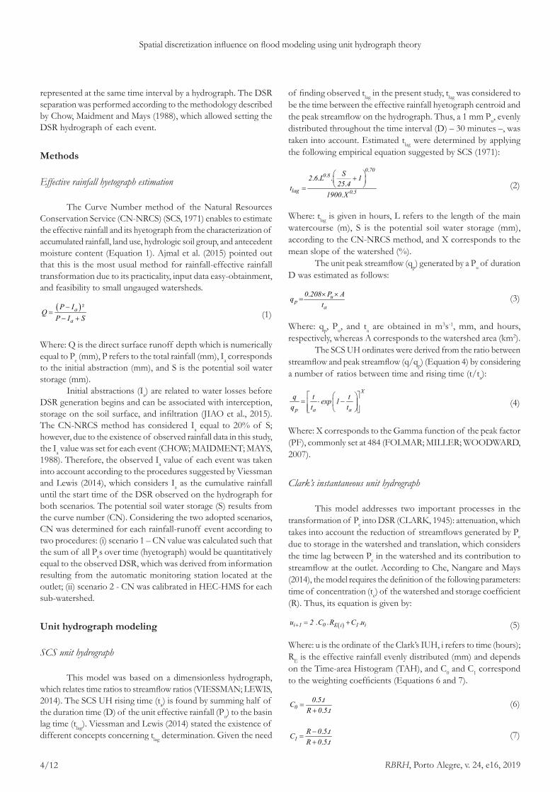
The CN-NRCS method, applied to convert rainfall into effective rainfall, and the two effective rainfall – streamflow transformation methods (SCS UH and Clark’s IUH) were herein assessed by considering two spatial discretization scenarios (Figure 2). All the procedures were carried out with the aid of the Hydrologic Modeling System (HEC-HMS), developed by the Hydrologic Engineering Center (HEC) of the Army Corps of Engineers (USACE, 2015).

Scenario 1 consists of the lumped modeling and scenario 2 follows a semi-distributed modeling approach (Figure 2). For the latter scenario, CRW was discretized into seven sub-watersheds (S1, S2, S3, S4, S5, S6, and S7) (Figure 1) in agreement with its drainage network. The parameters calibrated for both scenarios were tc and R (Clark’s IUH), while tlag and qp (SCS UH) were calculated according to equations 2 and 3, respectively. The calibration was intrinsic in HEC-HMS model structure for Clark’s IUH according to both scenarios and was similar to the one adopted by Joo et al. (2014), i.e. the Nelder and Mead algorithm (USACE, 2015) was employed

and assessed by an objective function named as root mean square error (RMSE).

Nelder and Mead algorithm

The HEC-HMS was calibrated by identifying optimal values for the Clark’s IUH parameters through minimization of the sum of squared residuals between observed and estimated hydrologic data (JOO et al., 2014). The Nelder and Mead algorithm searches for optimal values of these unknown parameters without using derivatives of the objective function to guide the search (USACE, 2015); instead, this algorithm relies on a simpler direct search. The Nelder and Mead search uses a simplex, in other words, a set of alternative parameters values (USACE, 2015). Lagarias et al. (1998) reported that the algorithm evolves a nondegenerate simplex, a geometric figure in n dimensions of nonzero volume and each iteration of a simplex based direct search method begins with a simplex to find vertex at which the value of the objective function is minimum.

Performance of the models

The performance of the models was quantified by application of the Nash-Sutcliffe coefficient (CNS) (NASH; SUTCLIFFE, 1970) (Equation 8), root mean square error (RMSE) (Equation 9), and percent mean relative error (PMRE) (Equation 10).

( )²

( )²obs est

obs obs

ni ii 1

NS ni ii 1

Q QC 1

Q Q=

=

−= −

−

∑∑

(8)

RMSE = ( )²obs est

ni ii 1 Q Qn

= −∑ (9)

Figure 2. Representation of the modeling elements in the HEC-HMS for the Cadeia river watershed (CRW) according to (a) scenario 1 (lumped approach) and (b) scenario 2 (semi-distributed approach) where the watershed was divided into seven sub-watersheds.

RBRH, Porto Alegre, v. 24, e16, 2019

Spatial discretization influence on flood modeling using unit hydrograph theory

6/12

PMRE = ( )est obs

obs

n i i

i 1 i

Q Q100n Q=

−∑ (10)

Where: obsiQ and estiQ are the observed and estimated streamflow

of the ith observation, respectively, Q is the average value of the observed streamflow, and n is the total number of observations.

RESULTS AND DISCUSSION

Scenario 1 (lumped approach)

The main characteristics of the eight rainfall-runoff events used for the scenario 1 are summarized in Table 2. Total rainfall ranged from 18.7 mm to 49.4 mm with duration of 18.0 h to 32.5 h; mean intensity varied between 0.8 mm h-1 and 1.9 mm h-1; effective rainfall had values from 2.1 mm to 12 mm with duration from 12.0 h to 25.5 h; and the 5-day antecedent rainfall presented values from 4.5 mm to 127.3 mm. Considering assessments associated with flood modeling, rainfall events with variable amounts have been used for analyses performed by various researchers over the world (GONZALO; ROBREDO; MINTEGUI, 2012; SADEGHI; MOSTAFAZADEH; SADODDIN, 2015; GHORBANI et al., 2017). Gonzalo, Robredo and Mintegui (2012) evaluated rainfall events with amounts ranging from 23.9 mm to 57.4 mm for a 131.4 km2 watershed, whereas, Sadeghi, Mostafazadeh and Sadoddin (2015) used events with depths from 2.4 mm to 33.11 in a drainage area of 103 km2. Ghorbani et al. (2017) made their analysis based on events with effective rainfall depths ranging from 0.04 mm to 1.35 mm. These authors employed events with magnitudes similar to those applied in this study or even with lower effective rainfall.

Although SCS (1971) recommends using tables to frame the CN (e.g. AHMAD; GHUMMAN; AHMAD, 2009; NGUYEN; MAATHUIS; RIENTJES, 2009; ŠRAJ; DIRNBEK; BRILLY, 2010), the methodology considered in the present study was to determine a CN for each event. These values varied considerably (from 61 to 97) among rainfall events, as well as Ia (from 3.9 to 28.9 mm), whereas, tabulated CN assumed the values of 53, 72 or 86 (Table 2). Considering estimated and tabulated CN

per event, its average value was similar between these approaches when evaluating all the events. However, estimated CN were different from those tabulated if analyzed per event (Table 2).

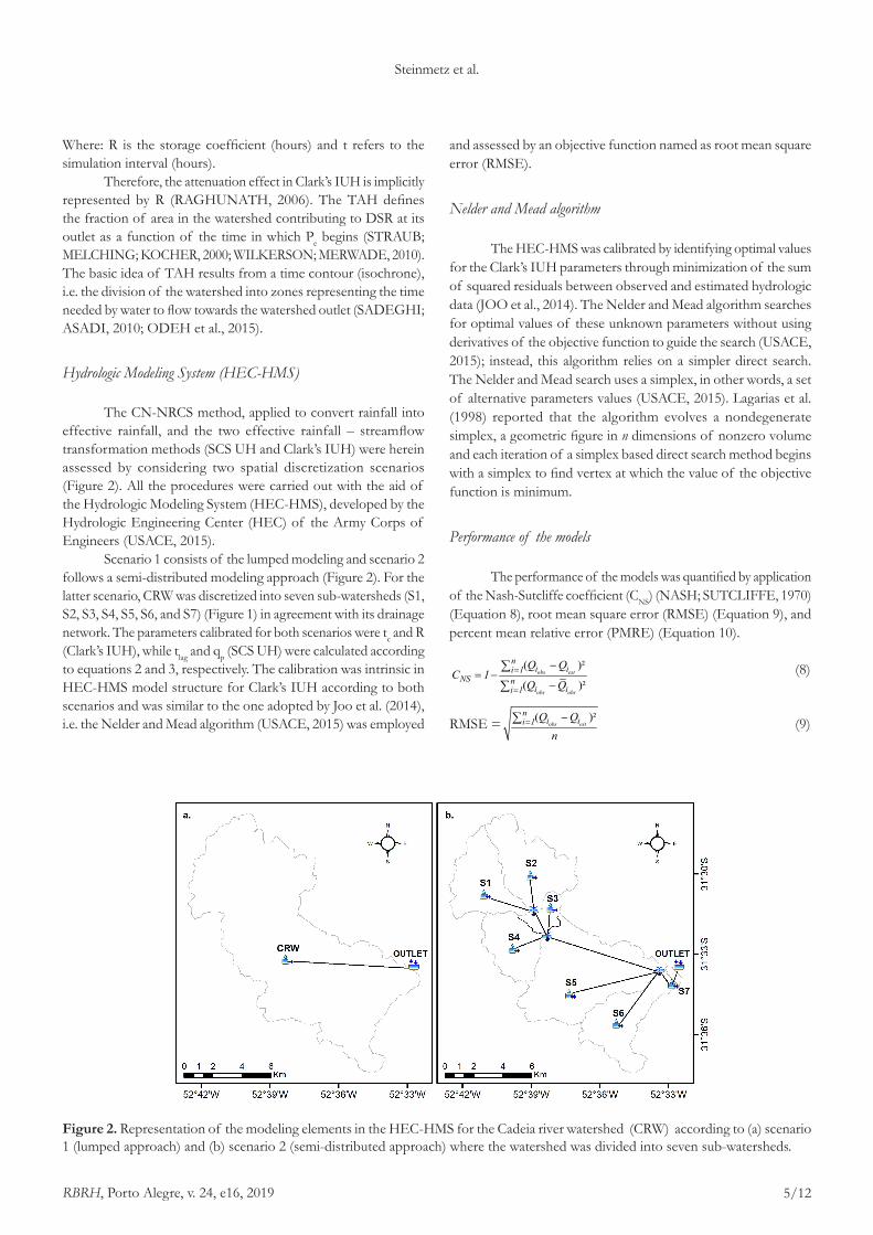
Since only one CN value is needed for each event in the lumped modeling (scenario 1), the same CN value was used for Clark’s IUH and SCS UH (Table 2). It is worth emphasizing that the adoption of the CN estimated per event assures that the total Pe will be numerically equal to the DSR monitored for the rainfall-runoff event. The use of tabulated CN would result in different values between Pe and the observed DSR, thereby causing errors in the UH model analyses. Thus, we analyzed the effective rainfall – streamflow transformation models and the influence exerted by the spatial discretization approach on their applicability. The estimated hydrographs using SCS UH and Clark’s IUH models, as well as the respective observed hydrograph of each event and analyzed scenario, are shown in Figure 3. In order to simplify the understanding and to provide a comparison between the assessed models, their precision statistics are compiled in Table 3.

It is possible to assume that the Clark’s IUH model outperformed SCS UH regarding the estimation of hydrographs for all the events in both scenarios (Figure 3). For both scenarios, peak streamflow was overestimated and anticipated in most events when derived from SCS UH. The PMRE (Table 3) was considerable high for the hydrographs estimated by SCS UH (34.4% to 137.1%) and for some events in the case of hydrographs derived from Clark’s IUH (26.8% to 85.1%). These high PMREs in events estimated by Clark’s IUH can be justified by the delay or anticipation of the estimated hydrographs in relation to the respective observed ones, thus generating errors in a couple of initial and final time steps. However, Clark’s IUH was able to adequately estimate the magnitude and timing of peak streamflows and of rising and recession limbs for all the hydrographs. In other words, PMRE was low for these situations, and such model could be therefore successfully used as a simplified tool for monitoring and early warning systems related to floods.

Relative to the Clark’s IUH parameters (tc and R), their fitted values to each analyzed event had a noticeable variation, e.g. tc ranged from 2.91 to 5.79 h and R presented values between 1.99 and 5.05 h (Table 4). Other studies have also evidenced a

Table 2. Characterization of the events applied to the flood modeling in scenario 1, with emphasis to the total rainfall for each event, total duration of rainfall event, mean intensity, effective rainfall, duration of effective rainfall, initial abstractions obtained by cumulative rainfall until the start time of the DSR observed on the hydrograph, 5-day antecedent rainfall, estimated Curve Number from Clark’s UH and tabulated Curve Number to determine the effective rainfall hyetographs according to CN-NRCS method (SCS, 1971).

Event PTOTAL (mm) DP (h) im (mm.h-1) Pe (mm) DPe (h) P5 (mm) Ia (mm) CN

estimated tabulated1 40.0 32.5 1.2 5.1 25.5 93.9 7.5 61 862 35.3 21.5 1.6 9.1 16.5 86.5 12.6 88 863 35.6 20.0 1.8 12.0 15.0 127.3 7.1 88 864 31.0 18.5 1.7 6.6 16.5 62.6 3.9 76 865 18.7 23.0 0.8 2.5 19.0 45.4 4.7 81 726 28.8 22.0 1.3 2.7 16.0 50.8 14.3 82 727 49.4 30.5 1.6 2.1 18.5 4.5 28.9 60 538 34.4 18.0 1.9 5.6 12.0 73.5 24.1 97 86

Average 34.2 23.3 1.5 5.7 17.4 68.1 12.9 79.4 78Note: PTOTAL = total rainfall; DP = total duration of rainfall event; im = mean intensity; Pe = effective rainfall; DPe = duration of effective rainfall; Ia = initial abstraction; P5 = 5-day antecedent rainfall; CN = Curve Number.

RBRH, Porto Alegre, v. 24, e16, 2019

Steinmetz et al.

7/12

Figure 3. Direct surface runoff hydrographs estimated from the SCS UH and Clark’s IUH models and the direct surface runoff hydrograph monitored at the Cadeia river watershed’s outlet for each analyzed event according to scenario 1 (lumped approach) and scenario 2 (semi-distributed approach).

Table 3. Values of the Nash-Sutcliffe, root mean square error (RMSE) and percent mean relative error (PMRE) statistics for each rainfall-runoff event analysed in this study, considering the unit hydrograph and instantaneous unit hydrograph models according to scenarios 1 and 2.

Event

Scenario 1

Event

Scenario 2Clark’s IUH SCS UH Clark’s IUH SCS UH

CNS

RMSE (m3.s-1)

PMRE (%) CNS

RMSE (m3.s-1)

PMRE (%) CNS

RMSE (m3.s-1)

PMRE (%) CNS

RMSE (m3.s-1)

PMRE (%)

1 0.96 1.12 69.1 0.83 2.40 77.3 1 0.97 0.97 71.7 -0.22 6.33 76.22 0.99 1.64 26.8 0.55 11.07 64.5 2 0.98 2.14 21.4 -1.07 23.61 142.53 0.98 3.00 59.5 -0.06 22.53 137.1 3 0.99 2.02 39.8 -3.11 44.32 594.34 0.98 1.67 35.4 0.86 4.27 34.4 4 0.99 1.18 23.0 -1.94 19.71 285.35 0.98 0.60 70.9 0.09 3.61 79.2 5 0.98 0.47 65.9 -2.65 7.21 174.86 0.96 0.96 85.1 0.66 2.74 112.3 6 0.97 0.83 67.2 -1.91 7.99 195.07 0.99 0.30 49.7 0.79 1.47 77.2 7 0.98 0.41 61.5 -1.12 4.68 178.68 0.96 2.67 62.9 0.50 9.14 81.6 8 0.99 1.55 103.0 -2.34 23.57 239.3

Note: CNS = Nash-Sutcliffe coefficient; RMSE = root mean square error; PMRE = percent mean relative error.

RBRH, Porto Alegre, v. 24, e16, 2019

Spatial discretization influence on flood modeling using unit hydrograph theory

8/12

notable variation (KUMAR et al., 2002; SAHOO et al., 2006; AHMAD; GHUMMAN; AHMAD, 2009; ADIB et al., 2010; YOO; KIM; YOON, 2012). Although equations often take fixed parameters into account to estimate tc, its value changes among events since it depends on characteristics that are not commonly included in these equations, such as magnitudes associated with rainfall and antecedent soil moisture. The parameter R represents a measure of Pe temporary storage in the watershed, before it reaches the outlet (YOO; KIM; YOON, 2012). The greater the R value in relation to tc, the stronger the effect of the temporary storage (detention) within the watershed (SABOL, 1988).

It is important to point out that the SCS UH application is considerably less complex, because it requires a smaller number of parameters which are easily acquired. As a result, SCS UH has been frequently adopted in hydrological engineering peak flood design (MAJIDI; MORADI; VAGHARFARD, 2012; LUXON; CHRISTOPHER; PIUS, 2013; SULE; ALABI, 2013; SILVA; WEERAKOON; HERATH, 2014; BESKOW et al., 2018). The tlag values were obtained by the SCS equation (Equation 2) based on watershed’s physiographic characteristics (Table 4) and on CN estimated per event (Table 2), taking the potential soil water storage (S) as variable. This procedure was also used by Soulis and Valiantzas (2012) and resulted in this study in tlag ranging from 1.62 to 5.60h (Table 4). It should be mentioned that Pus with the same intensity and duration culminated in discrepant tlag values; however, greater CN resulted in lower tlag and vice-versa. The aforementioned aspects resulted in poor performances of SCS UH model, suggesting that tlag may not have been adequately defined for this watershed. It should be also mentioned that CRW has a drainage area of approximately 120 km2, so considerable values of tlag are expected. In addition, it seems that tlag was in general underestimated, as the hydrographs estimated from SCS UH were anticipated in most of the events when compared to the observed hydrographs. We consider that the definition of tlag was the main reason that led to poor performances of the SCS UH model in this study.

The qp, which corresponds to the maximum unit streamflow of UH resulting from a Pu of duration D, varied from 4.20 to 12.61 m3.s-1 (Table 4). This parameter is also directly related to CN value. One can notice that the greatest qp and CN were observed in the same event, as well as the lowest qp and CN (Table 4). Accordingly, the lower the tlag, the greater the qp; thus, they are inversely proportional. For heavy rainfall, Costache (2014) stated that the lowest tlag showed that the accelerated flow and the water concentration would cause rapid routing of the flood downstream and an exponential increase in streamflow in the

short-term. Thus, lower tlag have indicated higher flood vulnerability in downstream areas within the watershed (MERAJ et al., 2015).

Besides the tlag, the accurate determination of peak streamflow of a watershed also depends on the peak factor and it is important for studies that employ SCS UH. According to Folmar, Miller and Woodward (2007), this factor can range from 300 (flat wetlands) to 600 (steep areas). The peak factor used in this study (Equation 4) was 484. This value is considered representative, but such choice may have impacted the SCS UH performance. We consider that the SCS UH can be further improved by considering different peak factors for CRW derived from a calibration procedure. Although the results found in this research have indicated that in-depth assessments regarding peak factor application are relevant, this analysis is beyond the scope of our study.

Scenario 2 (semi-distributed approach)

Results from the scenario 2 (Table 3) elucidate that the CIUH performance was slightly better than that found for scenario 1 in which the hydrographs estimated for all the events presented a good fit. This finding can be reinforced by the lower values of PMRE. However, different from scenario 1, the CNS and PMRE (76.2%-594.3%) results from the SCS UH showed worse performance. Similar to scenario 1, the CN calibration per sub-watershed was conducted along with the calibration of Clark’s IUH parameters for each event analyzed in the scenario 2, and the CN values were directly used to assess the SCS UH. It was possible to assume that Clark’s IUH superiority was likely associated with the use of observed rainfall and streamflow data sets during the calibration process, in agreement with Bhaskar, Parida and Nayak (1997), Adib et al. (2010), and Ahmad, Ghumman and Ahmad (2009).

Besides the considerable variation among sub-watersheds, scenario 2 suggested that CN values were also contrasting when evaluating different events for the same sub-watershed. Likewise, the Ia values were highly variable when they were analyzed among sub-watersheds, as well as in the same sub-watershed. However, this behavior was expected since Ia values were acquired from the average hyetograph of each sub-watershed. The differences between the tabulated and estimated CN in the scenario 2 were comparatively greater than those found in the scenario 1.

The Clark’s IUH parameters resulting from the calibration process for the scenario 2 made it possible to infer that tc and R values had considerable variation among sub-watersheds and events. On average, the greatest tc and R were found in S7, whereas the lowest values were verified in S4. Despite the excellent calibration

Table 4. Parameterization of Clark’s Instantaneous Unit Hydrograph and SCS Unit Hydrograph models in each analyzed event according to scenario 1 (lumped approach).

EventClark’s IUH SCS UH

EventClark’s IUH SCS UH

tc (h) R (h) tlag (h) qp (m3.s-1) tc (h) R (h) tlag (h) qp (m

3.s-1)1 2.91 5.05 5.39 4.20 5 5.79 4.05 3.13 6.302 4.07 3.13 2.46 8.41 6 5.19 2.86 3.03 7.213 4.42 3.77 2.48 8.41 7 3.99 4.44 5.60 4.204 4.98 3.56 3.65 6.30 8 2.95 1.99 1.62 12.61

Note: Clark’s IUH = Clark’s Instantaneous Unit Hydrograph; SCS UH = SCS Unit Hydrograph; tc = time of concentration; R = storage coefficient; tlag = basin lag time; qp = unit peak streamflow.

RBRH, Porto Alegre, v. 24, e16, 2019

Steinmetz et al.

9/12

in the scenario 2 through the Clark’s IUH, the model parameters often do not capture the hydrological behavior of the watershed. Therefore, it is recommended attention when calibrating this model for semi-distributed modeling purposes.

Considering SCS UH parameters in the scenario 2, S5 presented the greatest tlag in most of the events. This result can be explained by the fact that this sub-watershed has the longest main water course (15.2 km) and the largest drainage area (41.5 km2). Similarly, S7 presented the shortest main water course (1.3 km) and the smallest drainage area (0.7 km2), which justifies its lower tlag. These results are in agreement with Zhang et al. (2013), who mentioned that tlag increases proportionally as the watershed area increases. The greatest qp were identified in S5 in most of the events. Because qp is related to drainage area, such assumption is ratified by the fact that S5 has the largest area among the sub-watersheds. The same assumption about the lowest qp could be analyzed in S7, which presents the smallest drainage area. It is also important to point out the association between rising time (ta) and tlag and their relationship with qp, such that the lower the tlag, the lower the ta and the greater the qp.

Comparing scenarios (lumped approach versus semi-distributed approach)

It is worth highlighting that the SCS UH application for the scenario 1 led to good performance in 50% of the events. Other studies about SCS UH in the HEC-HMS have reported satisfactory results for the same spatial approach (ABUSHANDI; MERKEL, 2013; FOULI et al., 2016; IBRAHIM-BATHIS; AHMED, 2016; MASOUD, 2016). Researches approaching the semi-distributed modeling are rare. However, depending on the size of the watershed under analysis and on the rainfall spatial variation, this approach can be meaningful for water resources management.

Gonzalo, Robredo and Mintegui (2012) assessed the semi-distributed approach for flood analysis in a watershed in Costa Rica using the Clark’s IUH and SCS UH with the aid of HEC-HMS. Their results evidenced that Clark’s IUH generated more accurate hydrographs; however, the authors found that the application difficulties of this approach are related to the need of calibrating the parameters.

It is noticeable that SCS UH had worse performance in the scenario 2 (Table 3) and this behavior was expected. The uncertainty involved in CN determination in the scenario 2 was an aspect that might have influenced this behavior since the NRCS-CN method was not developed to consider time (WOODWARD et al., 2002). The method was thought to compute the total runoff volume from a watershed and this may be a reason of why it does not adjust easily to particular temporal rainfall patterns, or to watersheds which have a significant evolution of direct surface runoff in time (CAVIEDES-VOULLIÈME et al., 2012). Although NRCS-CN method has been developed for estimating direct surface runoff from single rainfall events, Woodward et al. (2002) stated that in practice it is frequently applied for daily rainfalls. Yet, these researchers mentioned that this method can be used for a continuous rainfall to compute the accumulated direct surface runoff. The aforementioned discussion provides a basis for justifying why the effective rainfall events normally had

long durations in this study. This can be attributed primarily to the long duration rainfall events; and secondly to the way how the NRCS-CN method determines the distribution of effective rainfalls over time, as it considers that any amount of rainfalls is able to generate effective rainfall after the moment that the initial abstractions are satisfied.

Differently from the scenario 2, CN value was estimated to have estimated Pe coincident with that observed for the scenario 1. Moreover, the number of calibration parameters per event is 2 and 21 for the lumped and semi-distributed scenarios, respectively. Therefore, it is evident the greater difficulties of the calibration process in the scenario 2. The calibration of CN per sub-watersheds may have increased the uncertainty level, thereby exerting negative impact on both tlag and model performance.

The Clark’s IUH parameters (tc and R) were estimated in each event as well. Thus, it is likely that the CN errors have been compensated by tc and R estimates, resulting in good performances in terms of DSR hydrograph estimates. Some difficulties observed during the HEC-HMS application are related to the calibration of model’s parameters. This can be attributed to the optimization algorithm, which has high sensitivity associated with initial values, and to the considerable number of calibration parameters for the scenario 2. This statement corroborates the assumptions by Abushandi and Merkel (2013), Laouacheria and Mansouri (2015) and Masoud (2016).

Regarding model calibration, there may not be even a unique set of parameters capable of representing the hydrological processes due to the uncertainties inherent to data, model simplification, and parameter representativeness. Under this context, the NM algorithm is somehow quite limited, so the researchers are encouraged to apply algorithms more appropriate to manage these issues. The results found in our study for the scenario 1 suggest that the NM algorithm in HEC-HMS culminated in coherent results under the hydrological point of view to the analyzed watershed. However, sometimes the results for the scenario 2 did not meet the reality in the watershed.

CONCLUSION

The main conclusions are:

• The Clark’s IUH was able to adequately estimate DSR hydrographs originated from intense rainfall, even for long duration rainfall events in the CRW;

• The spatial discretization in sub-watersheds generally did not lead to significant improvement in estimating DSR hydrographs in the CRW;

• In the semi-distributed approach, parameters were discretized and related to the physical reality of the watershed, providing awareness of the contribution from each sub-watershed;

• With regard to Clark’s IUH, the semi-distributed modeling resulted in slightly superior performance;

• The NM calibration algorithm may have limited application, mainly when it is applied to discretization by sub-watershed.

RBRH, Porto Alegre, v. 24, e16, 2019

Spatial discretization influence on flood modeling using unit hydrograph theory

10/12

ACKNOWLEDGEMENTS

The authors wish to thank Coordenação de Aperfeiçoamento de Pessoal de Nível Superior (CAPES) – Finance Code 001 for scholarship to the first author, Conselho Nacional de Desenvolvimento Científico e Tecnológico (CNPq) for financial support of this research and scholarship to the second author, and Fundação de Amparo à Pesquisa do Estado do Rio Grande do Sul (FAPERGS) for financial support of this research.

REFERENCES

ABUSHANDI, E.; MERKEL, B. Modelling rainfall runoff relations using HEC-HMS and IHACRES for a single rain event in an arid region of Jordan. Water Resources Management, v. 27, n. 7, p. 2391-2409, 2013. http://dx.doi.org/10.1007/s11269-013-0293-4.

ADIB, A.; SALARIJAZI, M.; VAGHEFI, M.; SHOOSHTARI, M. M.; AKHONDALI, A. M. Comparison between GcIUH-Clark, GIUH-Nash, Clark-IUH, and Nash-IUH models. Turkish Journal of Engineering and Environmental Sciences, v. 34, n. 2, p. 91-104, 2010.

AHMAD, M. M.; GHUMMAN, A. R.; AHMAD, S. Estimation of Clark’s instantaneous unit hydrograph parameters and development of direct surface runoff hydrograph. Water Resources Management, v. 23, n. 12, p. 2417-2435, 2009. http://dx.doi.org/10.1007/s11269-008-9388-8.

AHMAD, M. M.; GHUMMAN, A. R.; AHMAD, S.; HASHMI, H. N. Estimation of a unique pair of Nash model parameters: an optimization approach. Water Resources Management, v. 24, n. 12, p. 2971-2989, 2010. http://dx.doi.org/10.1007/s11269-010-9590-3.

AJMAL, M.; WASEEM, M.; AHN, J. H.; KIM, T. W. Improved runoff estimation using event-based rainfall-runoff models. Water Resources Management, v. 29, n. 6, p. 1995-2010, 2015. http://dx.doi.org/10.1007/s11269-015-0924-z.

BESKOW, S.; NUNES, G. S.; MELLO, C. R.; CALDEIRA, T. L.; NORTON, L. D.; STEINMETZ, A. A.; VARGAS, M. M.; ÁVILA, L. F. Geomorphology-based unit hydrograph models for flood risk management: case study in Brazilian watersheds with contrasting physiographic characteristics. Anais da Academia Brasileira de Ciências, v. 90, n. 2, p. 1873-1890, 2018. http://dx.doi.org/10.1590/0001-3765201820170430. PMid:29791526.

BHASKAR, N. R.; PARIDA, B. P.; NAYAK, A. K. Flood estimation for ungauged catchments using the GIUH. Journal of Water Resources Planning and Management, v. 123, n. 4, p. 228-238, 1997. http://dx.doi.org/10.1061/(ASCE)0733-9496(1997)123:4(228).

BRUNDA, G. S.; NYAMATHI, S. J.. Derivation and analysis of dimensionless hydrograph and S curve for cumulative watershed area. Aquatic Procedia, v. 4, p. 964-971, 2015. http://dx.doi.org/10.1016/j.aqpro.2015.02.121.

CAVIEDES-VOULLIÈME, D.; GARCÍA-NAVARRO, P.; MURILLO, J. Influence of mesh structure on 2D full shallow

water equations and SCS Curve Number simulation of rainfall/runoff events. Journal of Hydrology (Amsterdam), v. 448, p. 39-59, 2012. http://dx.doi.org/10.1016/j.jhydrol.2012.04.006.

CHE, D.; NANGARE, M.; MAYS, L. Determination of Clark’s Unit Hydrograph parameters for watersheds. Journal of Hydrologic Engineering, v. 19, n. 2, p. 384-387, 2014. http://dx.doi.org/10.1061/(ASCE)HE.1943-5584.0000796.

CHOW, V.; MAIDMENT, D.; MAYS, L. Applied hydrology. New York: McGraw-Hill, 1988.

CLARK, C. O. Storage and the unit hydrograph. Transactions of the American Society of Civil Engineers, v. 110, p. 1419-1488, 1945.

COSTACHE, R. Using GIS techniques for assessing lag time and concentration time in small river basins. Case study: Pecineaga river basin, Romania. Geographia Technica, v. 9, n. 1, p. 31-38, 2014.

DARIANE, A. B.; JAVADIANZADEH, M. M.; JAMES, L. D. Developing an efficient auto-calibration algorithm for HEC-HMS program. Water Resources Management, v. 30, n. 6, p. 1923-1937, 2016. http://dx.doi.org/10.1007/s11269-016-1260-7.

DU, S.; SHI, P.; VAN ROMPAEY, A.; WEN, J. Quantifying the impact of impervious surface location on flood peak discharge in urban areas. Natural Hazards, v. 76, n. 3, p. 1457-1471, 2015. http://dx.doi.org/10.1007/s11069-014-1463-2.

EMBRAPA – EMPRESA BRASILEIRA DE PESQUISA AGROPECUÁRIA. Estação Agroclimatológica de Pelotas. Pelotas: Convênio Embrapa/UFPEL, 2015.

ESRI – ENVIRONMENTAL SYSTEMS RESEARCH. ArcGIS DESKTOP 10.1. Redlands: Environmental Systems Research Institute, Inc., 2017. CD-ROM.

FOLMAR, N. D.; MILLER, A. C.; WOODWARD, D. E. History and development of the NRCS lag time equation. Journal of the American Water Resources Association, v. 43, n. 3, p. 829-838, 2007. http://dx.doi.org/10.1111/j.1752-1688.2007.00066.x.

FOULI, H.; AL-TURBAK, A. S.; BASHIR, B.; LONI, O. A. Assessment of a water-harvesting site in Riyadh Region of Kingdom of Saudi Arabia using hydrological analysis. Arabian Journal of Geosciences, v. 9, n. 5, p. 387, 2016. http://dx.doi.org/10.1007/s12517-016-2410-1.

GHORBANI, M. A.; SINGH, V. P.; SIVAKUMAR, B.; H. KASHANI, M.; ATRE, A. A.; ASADI, H. Probability distribution functions for unit hydrographs with optimization using genetic algorithm. Applied Water Science, v. 7, n. 2, p. 663-676, 2017. http://dx.doi.org/10.1007/s13201-015-0278-y.

GONZALO, C.; ROBREDO, J. C.; MINTEGUI, J. Á. Semidistributed hydrologic model for flood risk assessment in the Pejibaye River Basin, Costa Rica. Journal of Hydrologic Engineering, v. 17, n. 12, p.

RBRH, Porto Alegre, v. 24, e16, 2019

Steinmetz et al.

11/12

1333-1344, 2012. http://dx.doi.org/10.1061/(ASCE)HE.1943-5584.0000568.

HAO, F.; SUN, M.; GENG, X.; HUANG, W.; OUYANG, W. Coupling the Xinanjiang model with geomorphologic instantaneous unit hydrograph for flood forecasting in northeast China. International Soil and Water Conservation Research, v. 3, n. 1, p. 66-76, 2015. http://dx.doi.org/10.1016/j.iswcr.2015.03.004.

HASENACK, H.; WEBER, E. Base cartográfica vetorial continua do Rio Grande do Sul – escala 1:50.000. Porto Alegre: UFRGS/Centro de Ecologia, 2010. CD-ROM.

HUTCHINSON, M. F.; XU, T.; STEIN, J. A. Recent Progress in the ANUDEM Elevation Gridding Procedure. In: HENGEL, T., EVANS, I. S., WILSON, J. P., GOULD, M. (Ed.). Geomorphometry. California: Redlands, 2011. p. 19-22.

IBRAHIM-BATHIS, K.; AHMED, S. A. Rainfall-runoff modelling of Doddahalla watershed—an application of HEC-HMS and SCN-CN in ungauged agricultural watershed. Arabian Journal of Geosciences, v. 9, n. 3, p. 170, 2016. http://dx.doi.org/10.1007/s12517-015-2228-2.

JIAO, P.; XU, D.; WANG, S.; YU, Y.; HAN, S. Improved SCS-CN method based on storage and depletion of antecedent daily precipitation. Water Resources Management, v. 29, n. 13, p. 4753-4765, 2015. http://dx.doi.org/10.1007/s11269-015-1088-6.

JOO, J.; KJELDSEN, T.; KIM, H. J.; LEE, H. A comparison of two event-based flood models (ReFH-rainfall runoff model and HEC-HMS) at two Korean catchments, Bukil and Jeungpyeong. KSCE Journal of Civil Engineering, v. 18, n. 1, p. 330-343, 2014. http://dx.doi.org/10.1007/s12205-013-0348-3.

KUMAR, R.; CHATTERJEE, C.; LOHANI, A. K.; KUMAR, S.; SINGH, R. D. Sensitivity analysis of the GIUH based Clark model for a catchment. Water Resources Management, v. 16, n. 4, p. 263-278, 2002. http://dx.doi.org/10.1023/A:1021920717410.

LAGARIAS, J. C.; REEDS, J. A.; WRIGHT, M. H.; WRIGHT, P. E. Convergence properties of the Nelder--Mead simplex method in low dimensions. SIAM Journal on Optimization, v. 9, n. 1, p. 112-147, 1998. http://dx.doi.org/10.1137/S1052623496303470.

LAMPERT, D. J.; WU, M. Development of an open-source software package for watershed modeling with the Hydrological Simulation Program in Fortran. Environmental Modelling & Software, v. 68, p. 166-174, 2015. http://dx.doi.org/10.1016/j.envsoft.2015.02.018.

LAOUACHERIA, F.; MANSOURI, R. Comparison of WBNM and HEC-HMS for runoff hydrograph prediction in a small urban catchment. Water Resources Management, v. 29, n. 8, p. 2485-2501, 2015. http://dx.doi.org/10.1007/s11269-015-0953-7.

LUXON, N.; CHRISTOPHER, M.; PIUS, C. Validating the Soil Conservation Service triangular unit hydrograph (SCS-TUH) model in estimating runoff peak discharge of a catchment in Masvingo,

Zimbabwe. International Journal of Water Resources and Environmental Engineering, v. 5, n. 3, p. 157-162, 2013.

MAJIDI, A.; MORADI, M.; VAGHARFARD, H. Evaluation of Synthetic Unit Hydrograph (SCS) and Rational Methods in Peak Flow Estimation (case study: Khoshehaye Zarrin Watershed, Iran). International Journal of Hydraulic Engineering, v. 1, n. 5, p. 43-47, 2012.

MASOUD, M. H. Geoinformatics application for assessing the morphometric characteristics’ effect on hydrological response at watershed (case study of Wadi Qanunah, Saudi Arabia). Arabian Journal of Geosciences, v. 9, n. 4, p. 280, 2016. http://dx.doi.org/10.1007/s12517-015-2300-y.

MERAJ, G.; ROMSHOO, S. A.; YOUSUF, A. R.; ALTAF, S.; ALTAF, F. Assessing the influence of watershed characteristics on the flood vulnerability of Jhelum basin in Kashmir Himalaya. Natural Hazards, v. 77, n. 1, p. 153-175, 2015. http://dx.doi.org/10.1007/s11069-015-1605-1.

NASH, J. E.; SUTCLIFFE, J. V. River flow forecasting through conceptual models part I—A discussion of principles. Journal of Hydrology (Amsterdam), v. 10, n. 3, p. 282-290, 1970. http://dx.doi.org/10.1016/0022-1694(70)90255-6.

NGUYEN, H. Q.; MAATHUIS, B. H. P.; RIENTJES, T. H. M. Catchment storm runoff modelling using the geomorphologic instantaneous unit hydrograph. Geocarto International, v. 24, n. 5, p. 357-375, 2009. http://dx.doi.org/10.1080/10106040802677011.

ODEH, T.; RÖDIGER, T.; GEYER, S.; SCHIRMER, M. Hydrological modelling of a heterogeneous catchment using an integrated approach of remote sensing, a geographic information system and hydrologic response units: the case study of Wadi Zerka Ma’in catchment area, north east of the Dead Sea. Environmental Earth Sciences, v. 73, n. 7, p. 3309-3326, 2015. http://dx.doi.org/10.1007/s12665-014-3627-5.

RAGHUNATH, H. M. Hydrology: principles, analyses and design. New Delhi: New Age International, 2006.

RIVARD, C.; LEFEBVRE, R.; PARADIS, D. Regional recharge estimation using multiple methods: an application in the Annapolis Valley, Nova Scotia (Canada). Environmental Earth Sciences, v. 71, n. 3, p. 1389-1408, 2014. http://dx.doi.org/10.1007/s12665-013-2545-2.

SABOL, G. V. Clark unit hydrograph and R-parameter estimation. Journal of Hydraulic Engineering, v. 114, n. 1, p. 103-111, 1988. http://dx.doi.org/10.1061/(ASCE)0733-9429(1988)114:1(103).

SADEGHI, S. H. R.; ASADI, H. Importance of travel time duration between isochrones in estimation of flood resulting from Clark instantaneous unit hydrograph. Journal of Water and Soil, v. 24, n. 4, p. 625-635, 2010.

SADEGHI, S. H. R.; MOSTAFAZADEH, R.; SADODDIN, A. Changeability of simulated hydrograph from a steep watershed resulted from applying Clark’s IUH and different time–area

RBRH, Porto Alegre, v. 24, e16, 2019

Spatial discretization influence on flood modeling using unit hydrograph theory

12/12

histograms. Environmental Earth Sciences, v. 74, n. 4, p. 3629-3643, 2015. http://dx.doi.org/10.1007/s12665-015-4426-3.

SAHOO, B.; CHATTERJEE, C.; RAGHUWANSHI, N. S.; SINGH, R.; KUMAR, R. Flood estimation by GIUH-based Clark and Nash models. Journal of Hydrologic Engineering, v. 11, n. 6, p. 515-525, 2006. http://dx.doi.org/10.1061/(ASCE)1084-0699(2006)11:6(515).

SCS – SOIL CONSERVATION SERVICE. Hydrology. National Engineering Handbook. Washington : U.S. Dept. of Agriculture, 1971. Suppl A, section 4, chap. 10.

SILVA, M. M. G. T.; WEERAKOON, S. B.; HERATH, S. Modeling of event and continuous flow hydrographs with HEC–HMS: Case study in the Kelani River Basin, Sri Lanka. Journal of Hydrologic Engineering, v. 19, n. 4, p. 800-806, 2014. http://dx.doi.org/10.1061/(ASCE)HE.1943-5584.0000846.

SMITH, M. B.; KOREN, V. I.; ZHANG, Z.; REED, S. M.; PAN, J. J.; MOREDA, F. Runoff response to spatial variability in precipitation: an analysis of observed data. Journal of Hydrology (Amsterdam), v. 298, n. 1-4, p. 267-286, 2004. http://dx.doi.org/10.1016/j.jhydrol.2004.03.039.

SOULIS, K. X.; VALIANTZAS, J. D. SCS-CN parameter determination using rainfall-runoff data in heterogeneous watersheds-the two-CN system approach. Hydrology and Earth System Sciences, v. 16, n. 3, p. 1001-1015, 2012. http://dx.doi.org/10.5194/hess-16-1001-2012.

SPAROVEK, G.; VAN LIER, Q.; DOURADO NETO, D. Computer assisted Koeppen climate classification: a case study for Brazil. International Journal of Climatology, v. 27, n. 2, p. 257-266, 2007. http://dx.doi.org/10.1002/joc.1384.

ŠRAJ, M.; DIRNBEK, L.; BRILLY, M. The influence of effective rainfall on modeled runoff hydrograph. Journal of Hydrology and Hydromechanics, v. 58, n. 1, p. 3-14, 2010. http://dx.doi.org/10.2478/v10098-010-0001-5.

STEINMETZ, A. Estimativa de cheias aplicando a técnica de hidrograma unitário com diferentes abordagens de Discretização espacial em uma sub-bacia do arroio Pelotas. 2017. 109 f. Dissertação (Mestrado em Recursos Hídricos) - Universidade Federal de Pelotas, Pelotas, 2017.

STRAUB, T. D.; MELCHING, C. S.; KOCHER, K. E. Equations for estimating Clark unit-hydrograph parameters for small rural watersheds in Illinois. USA: USGS, 2000. U.S. Geological Survey Publication. https://doi.org/10.3133/wri004184.

SULE, B. F.; ALABI, S. A. Application of synthetic unit hydrograph methods to construct storm hydrographs. International Journal of Water Resources and Environmental Engineering, v. 5, n. 11, p. 639-647, 2013.

USACE – US ARMY CORPS OF ENGINEERS. Hydrologic Modeling System HEC-HMS Version 4.1. Washington: U. S. Army Corps of Engineers, 2015. Release Notes.

VIESSMAN, W.; LEWIS, G. L. Introduction to hydrology. New York: Thomas Y. Crowell Company Inc., 2014.

WAŁĘGA, A. Application of HEC-HMS programme for the reconstruction of a flood event in an uncontrolled basin/Zastosowanie programu HEC-HMS do odtworzenia wezbrania powodziowego w zlewni niekontrolowanej. Journal of Water and Land Development, v. 18, n. 9, p. 13-20, 2013. http://dx.doi.org/10.2478/jwld-2013-0002.

WILKERSON, J.; MERWADE, V. Incorporating surface storage and slope to estimate Clark unit hydrographs for ungauged Indiana watersheds. Journal of Hydrologic Engineering, v. 15, n. 11, p. 918-930, 2010. http://dx.doi.org/10.1061/(ASCE)HE.1943-5584.0000270.

WOODWARD, D.; HAWKINGS, R.; HJELMFELT, A.; VAN MULLEN, J.; QUAN, Q. Curve Number method: origins, applications and limitations. In: FEDERAL INTERAGENCY HYDROLOGIC MODELING CONFERENCE, 2., 2002, Las Vegas, Nevada. Proceedings… USA: ACWI, 2002.

YOO, C.; KIM, J.; YOON, J. Uncertainty of areal average rainfall and its effect on runoff simulation: a case study for the Chungju Dam Basin, Korea. KSCE Journal of Civil Engineering, v. 16, n. 6, p. 1085-1092, 2012. http://dx.doi.org/10.1007/s12205-012-1646-x.

ZHANG, H. L.; WANG, Y. J.; WANG, Y. Q.; LI, D. X.; WANG, X. K. The effect of watershed scale on HEC-HMS calibrated parameters: a case study in the Clear Creek watershed in Iowa, US. Hydrology and Earth System Sciences, v. 17, n. 7, p. 2735-2745, 2013. http://dx.doi.org/10.5194/hess-17-2735-2013.

Authors contributions

Alice Alonzo Steinmetz: Research, paper conception, data processing, data analysis, preparation of figures, literature review, discussion of results, paper writing.

Samuel Beskow: Paper conception, advisor professor, discussion of results, paper writing.

Fabrício da Silva Terra: Advisor researcher, discussion of results, manuscript revision.

Maria Cândida Moitinho Nunes: Advisor researcher, discussion of results, manuscript revision.

Marcelle Martins Vargas: Data processing, data analysis, preparation of graphs and figures, discussion of results, manuscript revision.

João Francisco Carlexo Horn: Advisor researcher, discussion of results, manuscript revision.