SPATIAL CONDITIONAL QUANTILE REGRESSION: WEAK CONSISTENCY ...€¦ · SPATIAL CONDITIONAL QUANTILE...
29
SPATIAL CONDITIONAL QUANTILE REGRESSION: WEAK CONSISTENCY OF A KERNEL ESTIMATE SOPHIE DABO-NIANG, ZOULIKHA KAID and ALI LAKSACI We consider a conditional quantile regression model for spatial data. More pre- cisely, given a strictly stationary random field Z i =(X i ,Y i ) i∈N N , we investigate a kernel estimate of the conditional quantile regression function of the univariate response variable Y i given the functional variable X i . The main purpose of the paper is to prove the convergence (with rate) in L p norm and the asymptotic normality of the estimator. AMS 2010 Subject Classification: 62M30, 62M20, 62G08, 62G05. Key words: Kernel conditional quantile estimation, Kernel regression estimation, spatial process. 1. INTRODUCTION Conditional quantile estimation is an important field in statistics which dates back to Stone (1977) and has been widely studied in the non-spatial case. It is useful in all domain of statistics, such as time series, survival ana- lysis and growth charts, among others, see Koenker ([20], [21]) for a review. There exist an extensive literature and various nonparametric approaches in conditional quantile estimation in the non spatial case for independent samples and dependent non-functional or functional observations. Among the many papers dealing with conditional quantile estimation in finite dimension, one can refer, for example, to key works of Portnoy [27], Koul and Mukherjee [23], Honda [19]. Potential applications of quantile regression to spatial data are number less. Indeed, there is an increasing number of situations coming from different fields of applied sciences (soil science, geology, oceanography, econometrics, epidemiology, environmental science, forestry, etc.), where the influence of a vector of covariates on some response variable is to be studied in a context of spatial dependence. The literature on spatial models is relatively abundant, see for example, Guyon [15], Anselin and Florax [3], Cressie [7] or Ripley [29] for a list of references. REV. ROUMAINE MATH. PURES APPL., 57 (2012), 4, 311-339
Transcript of SPATIAL CONDITIONAL QUANTILE REGRESSION: WEAK CONSISTENCY ...€¦ · SPATIAL CONDITIONAL QUANTILE...

SPATIAL CONDITIONAL QUANTILE REGRESSION:WEAK CONSISTENCY OF A KERNEL ESTIMATE
SOPHIE DABO-NIANG, ZOULIKHA KAID and ALI LAKSACI
We consider a conditional quantile regression model for spatial data. More pre-cisely, given a strictly stationary random field Zi = (Xi, Yi)i∈NN , we investigatea kernel estimate of the conditional quantile regression function of the univariateresponse variable Yi given the functional variable Xi. The main purpose of thepaper is to prove the convergence (with rate) in Lp norm and the asymptoticnormality of the estimator.
AMS 2010 Subject Classification: 62M30, 62M20, 62G08, 62G05.
Key words: Kernel conditional quantile estimation, Kernel regression estimation,spatial process.
1. INTRODUCTION
Conditional quantile estimation is an important field in statistics whichdates back to Stone (1977) and has been widely studied in the non-spatialcase. It is useful in all domain of statistics, such as time series, survival ana-lysis and growth charts, among others, see Koenker ([20], [21]) for a review.There exist an extensive literature and various nonparametric approaches inconditional quantile estimation in the non spatial case for independent samplesand dependent non-functional or functional observations. Among the manypapers dealing with conditional quantile estimation in finite dimension, onecan refer, for example, to key works of Portnoy [27], Koul and Mukherjee [23],Honda [19].
Potential applications of quantile regression to spatial data are numberless. Indeed, there is an increasing number of situations coming from differentfields of applied sciences (soil science, geology, oceanography, econometrics,epidemiology, environmental science, forestry, etc.), where the influence of avector of covariates on some response variable is to be studied in a context ofspatial dependence. The literature on spatial models is relatively abundant,see for example, Guyon [15], Anselin and Florax [3], Cressie [7] or Ripley [29]for a list of references.
REV. ROUMAINE MATH. PURES APPL., 57 (2012), 4, 311-339
312 Sophie Dabo-Niang, Zoulikha Kaid and Ali Laksaci 2
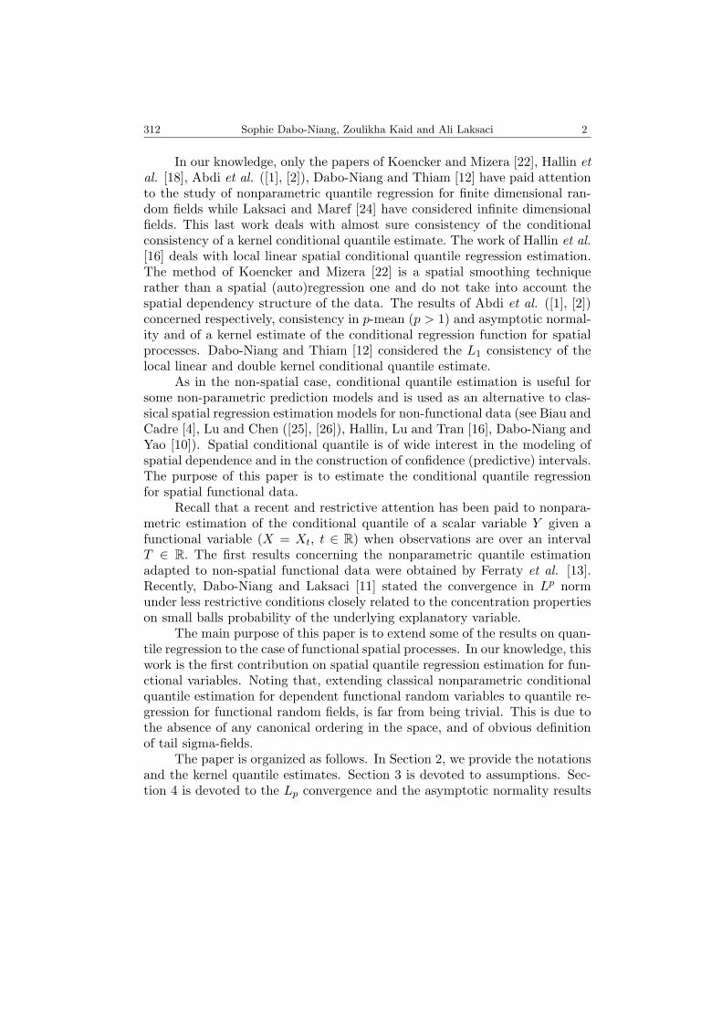
In our knowledge, only the papers of Koencker and Mizera [22], Hallin etal. [18], Abdi et al. ([1], [2]), Dabo-Niang and Thiam [12] have paid attentionto the study of nonparametric quantile regression for finite dimensional ran-dom fields while Laksaci and Maref [24] have considered infinite dimensionalfields. This last work deals with almost sure consistency of the conditionalconsistency of a kernel conditional quantile estimate. The work of Hallin et al.[16] deals with local linear spatial conditional quantile regression estimation.The method of Koencker and Mizera [22] is a spatial smoothing techniquerather than a spatial (auto)regression one and do not take into account thespatial dependency structure of the data. The results of Abdi et al. ([1], [2])concerned respectively, consistency in p-mean (p > 1) and asymptotic normal-ity and of a kernel estimate of the conditional regression function for spatialprocesses. Dabo-Niang and Thiam [12] considered the L1 consistency of thelocal linear and double kernel conditional quantile estimate.
As in the non-spatial case, conditional quantile estimation is useful forsome non-parametric prediction models and is used as an alternative to clas-sical spatial regression estimation models for non-functional data (see Biau andCadre [4], Lu and Chen ([25], [26]), Hallin, Lu and Tran [16], Dabo-Niang andYao [10]). Spatial conditional quantile is of wide interest in the modeling ofspatial dependence and in the construction of confidence (predictive) intervals.The purpose of this paper is to estimate the conditional quantile regressionfor spatial functional data.
Recall that a recent and restrictive attention has been paid to nonpara-metric estimation of the conditional quantile of a scalar variable Y given afunctional variable (X = Xt, t ∈ R) when observations are over an intervalT ∈ R. The first results concerning the nonparametric quantile estimationadapted to non-spatial functional data were obtained by Ferraty et al. [13].Recently, Dabo-Niang and Laksaci [11] stated the convergence in Lp normunder less restrictive conditions closely related to the concentration propertieson small balls probability of the underlying explanatory variable.
The main purpose of this paper is to extend some of the results on quan-tile regression to the case of functional spatial processes. In our knowledge, thiswork is the first contribution on spatial quantile regression estimation for fun-ctional variables. Noting that, extending classical nonparametric conditionalquantile estimation for dependent functional random variables to quantile re-gression for functional random fields, is far from being trivial. This is due tothe absence of any canonical ordering in the space, and of obvious definitionof tail sigma-fields.
The paper is organized as follows. In Section 2, we provide the notationsand the kernel quantile estimates. Section 3 is devoted to assumptions. Sec-tion 4 is devoted to the Lp convergence and the asymptotic normality results

3 Spatial conditional quantile regression 313
of the kernel quantile regression estimate, under mixing assumptions. Proofsand technical lemmas are given in Section 5.
2. THE MODEL
Consider Zi = (Xi, Yi), i ∈ NN be a F × R-valued measurable strictlystationary spatial process, defined on a probability space (Ω, A,P), where(F , d) is a semi-metric space. Let d denotes the semi-metric and N ≥ 1. Apoint i = (i1, . . . , iN ) ∈ NN will be referred to as a site. We assume that theprocess under study (Zi) is observed over a rectangular domain In = i =(i1, . . . , iN ) ∈ ZN , 1 ≤ ik ≤ nk, k = 1, . . . , N, n = (n1, . . . , nN ) ∈ NN . Apoint i will be referred to as a site. We will write n → ∞ if minnk → ∞and |nj
nk| < C for a constant C such that 0 < C < ∞, for all j, k such that
1 ≤ j, k ≤ N . For n = (n1, . . . , nN ) ∈ NN , we set n = n1 × · · · × nN .We assume that the Zi’s have the same distribution as (X,Y ) and the
regular version of the conditional probability of Y given X exists and admitsa bounded probability density. For all x ∈ F , we denote respectively by F x
and fx the conditional distribution function and density of Y given X = x.Let α ∈ ]0, 1[, the αth conditional quantile noted qα(x) is defined by
F x(qα(x)) = α.
To insure existence and unicity of qα(x), we assume that F x is strictlyincreasing. This last is estimated by
(1) F xn (y) =
∑i∈In
K1
(d(x,Xi)
an
)K2
(y−Yibn
)∑
i∈InK1
(d(x,Xi)
an
) if∑
i∈InK1
(d(x,Xi)
an
)6= 0,
0 else,
where K1 is a kernel, K2 is a distribution function, an (resp. bn) is a sequenceof real numbers which converges to 0 when n →∞.
The kernel estimate qα(x) of the conditional quantile qα(x) defined by
F x(qα(x)) = α.
One can also use other methods to estimate qα, such as the local linearmethod or the reproducing kernel Hilbert spaces method (see Preda, [28]).
In the following, we fix a point x in F such that
P (X ∈ B(x, r)) = φx(r) > 0,
where B(x, h) = x′ ∈ F | d(x′, x) < h.
314 Sophie Dabo-Niang, Zoulikha Kaid and Ali Laksaci 4
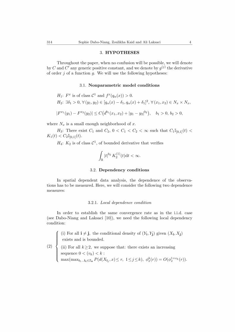
3. HYPOTHESES
Throughout the paper, when no confusion will be possible, we will denoteby C and C ′ any generic positive constant, and we denote by g(j) the derivativeof order j of a function g. We will use the following hypotheses:
3.1. Nonparametric model conditions
H1: F x is of class C1 and fx(qα(x)) > 0.
H2: ∃δ1 > 0, ∀ (y1, y2) ∈ [qα(x)− δ1, qα(x) + δ1]2, ∀ (x1, x2) ∈ Nx ×Nx,
|F x1(y1)− F x2(y2)| ≤ C(db1(x1, x2) + |y1 − y2|b2
), b1 > 0, b2 > 0,
where Nx is a small enough neighborhood of x.
H3: There exist C1 and C2, 0 < C1 < C2 < ∞ such that C1I[0,1](t) <K1(t) < C2I[0,1](t).
H4: K2 is of class C1, of bounded derivative that verifies∫R|t|b2 K(1)
2 (t)dt <∞.
3.2. Dependency conditions
In spatial dependent data analysis, the dependence of the observa-tions has to be measured. Here, we will consider the following two dependencemeasures:
3.2.1. Local dependence condition
In order to establish the same convergence rate as in the i.i.d. case(see Dabo-Niang and Laksaci [10]), we need the following local dependencycondition:
(2)
(i) For all i 6= j, the conditional density of (Yi, Yj) given (Xi, Xj)exists and is bounded.
(ii) For all k≥2, we suppose that: there exists an increasingsequence 0 < (vk) < k :max(maxi1...ik∈In P (d(Xij , x)≤ r, 1≤j≤k), φk
x(r)) = O(φ1+vkx (r)).

5 Spatial conditional quantile regression 315
3.2.2. Mixing condition
The spatial dependence of the process will be measured by means of α-mixing. Then, we consider the α-mixing coefficients of the field (Zi, i ∈ NN ),defined by: there exists a function ϕ(t) ↓ 0 as t→∞, such that whenever E,E′ subsets of NN with finite cardinals,
α(B(E), B(E′)) = supB∈B(E), C∈B(E′)
|P(B ∩ C)−P(B)P(C)|(3)
≤ ψ(Card(E),Card(E′))ϕ(dist(E,E′)),
where B(E) (resp. B(E′)) denotes the Borel σ-field generated by (Xi, i ∈ E)(resp. (Xi, i ∈ E′)), Card(E) (resp. Card(E′)) the cardinality of E (resp. E′),dist(E,E′) the Euclidean distance between E and E′ and ψ : N2 → R+ is asymmetric positive function nondecreasing in each variable.
Throughout the paper, it will be assumed that ψ satisfies either
(4) ψ(n,m) ≤ Cmin(n,m), ∀n,m ∈ N
or
(5) ψ(n,m) ≤ C(n+m+ 1)β, ∀n,m ∈ N
for some β ≥ 1 and some C > 0. In the following, we will only considerCondition (4), one can extend easily the asymptotic results proved here in thecase of (5).
We assume also that the process satisfies the following mixing condition:the process satisfies a polynomial mixing condition
(6)∞∑i=1
iδϕ(i) <∞, δ > N(p+ 2), p ≥ 1.
If N = 1, then Xi is called strongly mixing. Many stochastic processes,among them various useful time series models, satisfy strong mixing properties,which are relatively easy to check. Conditions (4)–(5) are used in Tran [30],Carbon et al. [5], and are satisfied by many spatial models (see Guyon [14] forsome examples). In addition, we assume that
H5: ∃0 < τ < (δ − 5N)/2N , η0, η1 > 0, such that nτ bn →∞ and
Cn(5+2τ)N−δ
δ+η0 ≤ φx(an),
where δ is introduced in (6).
Remark 1. If (6) is satisfied, then ϕ(i) ≤ Ci−δ.

316 Sophie Dabo-Niang, Zoulikha Kaid and Ali Laksaci 6
4. MAIN RESULTS
4.1. Weak consistency
This section contains results on pointwise consistency in p-mean. Let xbe fixed, we give a rate of convergence of qα (x) to qα (x) under some generalconditions.
Theorem 1. Under the hypotheses H1–H5, (4), then, for all p ≥ 1,we have
‖qα(x)− qα(x)‖p = (E|qα(x)− qα(x)|p)1/p =
= O((an)b1 + (bn)b2
)+O
((1
nφx(an)
) 12
).
Let
Ki = K1
(d(x,Xi)an
), Hi(y) = K2
(y − Yi
bn
), Wni = Wni(x) =
Ki∑i∈In Ki
,
F xN (y) =
1nEK1
∑i∈In
KiHi(y), F xD =
1nEK1
∑i∈In
Ki.
By hypothesis H4, F xN (y) is of class C1; then, we can write the following Taylor
development
F xN (qα(x)) = F x
N (qα(x)) + F x(1)
N (q∗α(x)) (qα(x)− qα(x)) ,
where q∗α(x) is in the interval of extremities qα(x) and qα(x). Thus,
qα(x)− qα(x) =1
F x(1)
N
(q∗α(x)
) (F xN
(qα(x)
)− F x
N
(qα(x)
))=
1
F x(1)
N
(q∗α(x)
) (αF xD − F x
N
(qα(x)
)).
It is shown in Laksaci and Maref (2009) that under (H1)–(H5), (2) and (6) that
qα(x)− qα(x) → 0, almost completely (a.co).
So, by combining this consistency and the result of Lemma 11.17 inFerraty and Vieu ([13], p. 181), together with the fact that q∗α(x) is lyingbetween qα(x) and qα(x), it follows that
(7) F x(1)
N (q∗α(x))− fx(qα(x)) → 0. a.co.

7 Spatial conditional quantile regression 317
Since fx(qα(x)) > 0, we can write
∃C > 0 such that
∣∣∣∣∣ 1
F x(1)
N (q∗α(x))
∣∣∣∣∣ ≤ C a.s.
It follows that
‖qα(x)− qα(x)‖p ≤ C∥∥αF x
D − F xN (qα(x))
∥∥p+(P (F x
D = 0))1/p
.
So, the rest of the proof is deduce from the following three lemmas.
Lemma 1. Under H2 −H4, we have
E[αF x
D − F xN (qα(x))
]= O
(ab1n + bb2n
).
Lemma 2. Under the hypotheses of Theorem 1, we have∥∥∥αF xD − F x
N (qα(x))− E[αF x
D − F xN (qα(x))
]∥∥∥p
= o
((1
nφx(an)
) 12
).
Lemma 3. Under the hypotheses of Lemma 2, we have(P(F x
D = 0))1/p
= o
((1
nφx(an)
) 12
).
4.2. Asymptotic normality
This section contains results on the asymptotic normality of the quan-tile estimator. For that we replace, respectively H2 and H4 by the followinghypotheses.
H ′2: F
x satisfies H2 and ∀z ∈ Nx, F z is of class C1 with respect to y,the conditional density fx is such that fx(qα) > 0 and ∀(x1, x2) ∈ Nx × Nx,∀(y1, y2) ∈ R2
|fx1(y1)− fx2(y2)| ≤(‖x1 − x2‖d1 + |y1 − y2|d2
), d1, d2 > 0.
H ′4: K2 satisfies H4 and∫
|t|d2K(1)2 (t)dt <∞.
Theorem 2. Under the hypotheses of Theorem 1 and H ′2, H
′4, (4) then,
for any x ∈ A, we have((fx(qα(x)))2n(ψK1(an))2
ψK21(an)(α(1− α))
)(1/2)
(qα(x)− qα(x)− Cn(x)) →n→+∞ N(0, 1),
318 Sophie Dabo-Niang, Zoulikha Kaid and Ali Laksaci 8
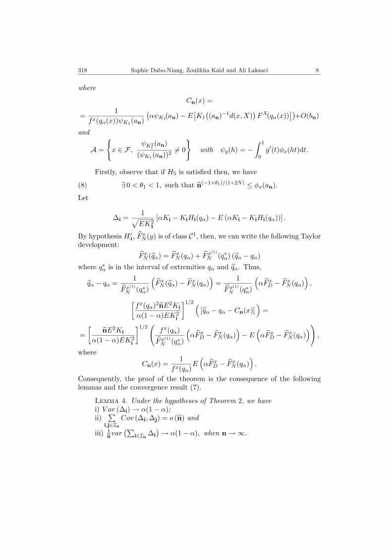
where
Cn(x) =
=1
fx(qα(x))ψK1(an)(αψK1(an)− E
[K1
((an)−1d(x,X)
)FX(qα(x))
])+O(bn)
and
A =
x ∈ F ,
ψK21(an)
(ψK1(an))26= 0
with ψg(h) = −
∫ 1
0g′(t)φx(ht)dt.
Firstly, observe that if H5 is satisfied then, we have
(8) ∃ 0 < θ1 < 1, such that n(−1+θ1)/(1+2N) ≤ φx(an).
Let
∆i =1√EK2
1
[αKi −KiHi(qα)− E (αKi −KiHi(qα))] .
By hypothesis H ′4, F
xN (y) is of class C1, then, we can write the following Taylor
development:
F xN (qα) = F x
N (qα) + F x(1)
N (q∗α) (qα − qα)
where q∗α is in the interval of extremities qα and qα. Thus,
qα − qα =1
F x(1)
N (q∗α)
(F x
N (qα)− F xN (qα)
)=
1
F x(1)
N (q∗α)
(αF x
D − F xN (qα)
),
[fx(qα)2nE2Ki
α(1− α)EK2i
]1/2 ([qα − qα − Cn(x)]
)=
=[
nE2Ki
α(1− α)EK2i
]1/2(
fx(qα)
F x(1)
N (q∗α)
(αF x
D − F xN (qα)
)− E
(αF x
D − F xN (qα)
)),
where
Cn(x) =1
fx(qα)E(αF x
D − F xN (qα)
).
Consequently, the proof of the theorem is the consequence of the followinglemmas and the convergence result (7).
Lemma 4. Under the hypotheses of Theorem 2, we havei) V ar (∆i) → α(1− α);ii)
∑i,j∈In
Cov (∆i,∆j) = o (n) and
iii) 1nvar
(∑i∈In ∆i
)→ α(1− α), when n →∞.

9 Spatial conditional quantile regression 319
Lemma 5. Under the hypotheses of Theorem 2 we have[nE2Ki
α(1− α)EK2i
]1/2 ([αF x
D − F xN (qα)
]− E
[αF x
D − F xN (qα)
])→ N(0, 1).
Lemma 6. Under the hypotheses H ′2 and H ′
4, we have
E[αF x
D − F xN (qα)
]= α− 1
EKiE
[K
(d, x−X
an
)FX(qα)
]+O
(bb2n
)and
E[αF x
D − F xN (qα)
]= O
(ab1n + bb2n
).
It is easy to see that, if one imposes some additional assumptions on thefunction φx(·) and the bandwidth parameters (an and bn) we can improved ourasymptotic normality by explicit asymptotic expressions of dispersion termsor by removing the bias term Cn(x).
Corollary 1. Under the hypotheses of Theorem 2 and if the bandwidthparameters (an and bn) and if the function φx(an) satisfies
limn→∞
(anb1 + bnb2)√
nφx(an) = 0 and limn→∞
φx(tan)φx(an)
= β(t), ∀t ∈ [0, 1],
we have((fx(tα(x)))2δ21δ2(α(1− α))
)(1/2)√nφx(an)
(tα(x)− tα(x)
)→n→+∞ N(0, 1),
where δj = −∫ 10 (Kj)′(s)β(s)ds, for, j = 1, 2.
Remark 2. If we assume that (5) is satisfied instead of (4) then it issimple to have the results of Theorems 1 and 2, the only thing that changes iscondition (H5) which will be replaced by some assumption that depend on β.
5. APPENDIX
We first state the following lemmas which are due to Carbon et al. [6].They are needed for the convergence of our estimates. Their proofs will thenbe omitted.
Lemma 7. Suppose E1, . . . , Er be sets containing m sites each withdist(Ei, Ej) ≥ γ for all i 6= j, where 1 ≤ i ≤ r and 1 ≤ j ≤ r. Sup-pose Z1, . . . , Zr is a sequence of real-valued r.v.’s measurable with respect toB(E1), . . . ,B(Er) respectively, and Zi takes values in [a, b]. Then, there ex-ists a sequence of independent r.v.’s Z∗
1 , . . . , Z∗r independent of Z1, . . . , Zr such

320 Sophie Dabo-Niang, Zoulikha Kaid and Ali Laksaci 10
that Z∗i has the same distribution as Zi and satisfies
r∑i=1
E|Zi − Z∗i | ≤ 2r(b− a)ψ((r − 1)m,m)ϕ(γ).
Lemma 8. (i) Suppose that (3) holds. Denote by Lr(F) the class ofF-measurable r.v.’s X satisfying ‖X‖r = (E|X|r)1/r < ∞. Suppose X ∈Lr(B(E)) and Y ∈ Ls(B(E′)). Assume also that 1 ≤ r, s, t < ∞ andr−1 + s−1 + t−1 = 1. Then,
|EXY − EXEY | ≤(9)
≤ C‖X‖r‖Y ‖sψ(Card(E), Card(E′))ϕ(dist(E,E′))1/t.
(ii) For r.v.’s bounded with probability 1, the right-hand side of (9) canbe replaced by Cψ(Card(E), Card(E′))ϕ(dist(E,E′)).
Proof of Lemma 1. We have
E[αF xD − F x
N (qα(x))] = α− 1EK1
(E [K1E [H1(qα(x)) | X1]]) .
We shall use the integration by parts and the usual change of variables t = y−zbn
,to show that
E[αF xD − F x
N (qα(x))] = α− 1EK1
(EK1
∫K
(1)2 (t)FX1((qα(x))− bnt)dt
).
Hypotheses (H2) and (H4) allow to get
E[αF xD − F x
N (qα(x))] ≤1
EK1E
[K1
∫K
(1)2 (t)
∣∣F x((qα(x))− FX1((qα(x))− bnt)dt∣∣] ≤ C
(ab1n + bb2n
).
Proof of Lemma 2. We have∥∥∥αF xD − F x
N (qα(x))− E[αF x
D − F xN (qα(x))
]∥∥∥p
=1
nEK1
∥∥∥∥∑i∈In
θi
∥∥∥∥p
,
whereθi = Ki(α−Hi(qα(x)))− E [Ki(α−Hi(qα(x)))] .
We have EK1 = O(φx(hK)), (because of H3), so it remains to show that∥∥∥∥∑i∈In
θi
∥∥∥∥p
= O(√
nφx(an)).
The evaluation of this quantity is based on ideas similar to that used by Gaoet al. (2008), see also Abdi et al. (2010). More preciously, we prove the case
11 Spatial conditional quantile regression 321
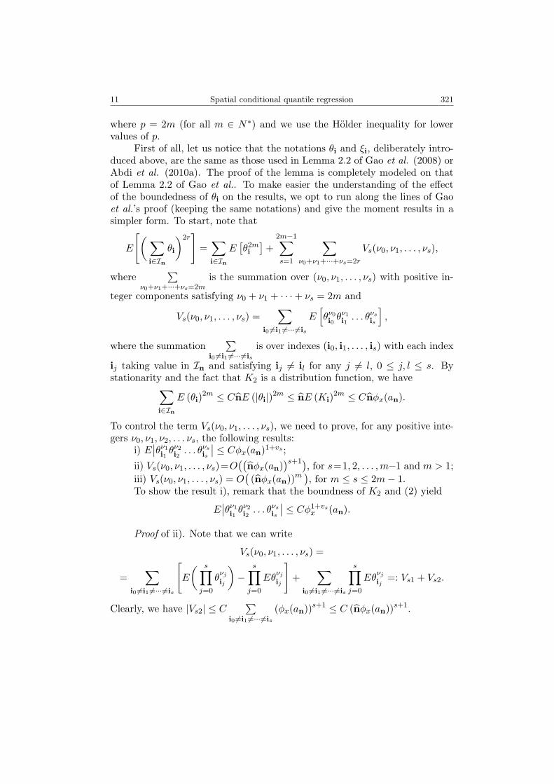
where p = 2m (for all m ∈ N∗) and we use the Holder inequality for lowervalues of p.
First of all, let us notice that the notations θi and ξi, deliberately intro-duced above, are the same as those used in Lemma 2.2 of Gao et al. (2008) orAbdi et al. (2010a). The proof of the lemma is completely modeled on thatof Lemma 2.2 of Gao et al.. To make easier the understanding of the effectof the boundedness of θi on the results, we opt to run along the lines of Gaoet al.’s proof (keeping the same notations) and give the moment results in asimpler form. To start, note that
E
[(∑i∈In
θi
)2r]
=∑i∈In
E[θ2mi
]+
2m−1∑s=1
∑ν0+ν1+···+νs=2r
Vs(ν0, ν1, . . . , νs),
where∑
ν0+ν1+···+νs=2mis the summation over (ν0, ν1, . . . , νs) with positive in-
teger components satisfying ν0 + ν1 + · · ·+ νs = 2m and
Vs(ν0, ν1, . . . , νs) =∑
i0 6=i1 6=···6=is
E[θν0i0θν1i1. . . θνs
is
],
where the summation∑
i0 6=i1 6=···6=is
is over indexes (i0, i1, . . . , is) with each index
ij taking value in In and satisfying ij 6= il for any j 6= l, 0 ≤ j, l ≤ s. Bystationarity and the fact that K2 is a distribution function, we have∑
i∈In
E (θi)2m ≤ CnE (|θi|)2m ≤ nE (Ki)
2m ≤ Cnφx(an).
To control the term Vs(ν0, ν1, . . . , νs), we need to prove, for any positive inte-gers ν0, ν1, ν2, . . . νs, the following results:
i) E∣∣θν1
i1θν2i2. . . θνs
is
∣∣ ≤ Cφx(an)1+vs ;
ii) Vs(ν0, ν1, . . . , νs)=O((
nφx(an))s+1), for s=1, 2, . . . ,m−1 and m > 1;
iii) Vs(ν0, ν1, . . . , νs) = O((nφx(an))m ), for m ≤ s ≤ 2m− 1.
To show the result i), remark that the boundness of K2 and (2) yield
E∣∣θν1
i1θν2i2. . . θνs
is
∣∣ ≤ Cφ1+vsx (an).
Proof of ii). Note that we can write
Vs(ν0, ν1, . . . , νs) =
=∑
i0 6=i1 6=···6=is
[E
( s∏j=0
θνj
ij
)−
s∏j=0
Eθνj
ij
]+
∑i0 6=i1 6=···6=is
s∏j=0
Eθνj
ij=: Vs1 + Vs2.
Clearly, we have |Vs2| ≤ C∑
i0 6=i1 6=···6=is
(φx(an))s+1 ≤ C (nφx(an))s+1.
322 Sophie Dabo-Niang, Zoulikha Kaid and Ali Laksaci 12
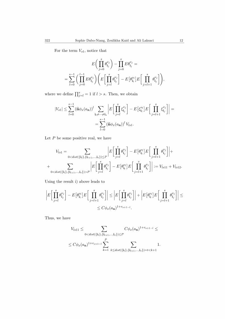
For the term Vs1, notice that
E
( s∏j=0
θνj
ij
)−
s∏j=0
Eθνj
ij=
=s−1∑l=0
( l−1∏j=0
Eθνj
ij
)(E
[ s∏j=l
θνj
ij
]− E
[θνlil
]E
[ s∏j=l+1
θνj
ij
]),
where we define∏s
j=l = 1 if l > s. Then, we obtain
|Vs1| ≤s−1∑l=0
(nφx(an))l∑
il 6=···6=is
∣∣∣∣E[ s∏j=l
ξνj
ij
]− E
[ξνlil
]E
[ s∏j=l+1
ξνj
ij
]∣∣∣∣ ==
s−1∑l=0
(nφx(an))l Vls1.
Let P be some positive real, we have
Vls1 =∑
0<dist(il,il+1,...,is)≤P
∣∣∣∣E[ s∏j=l
θνj
ij
]− E
[θνlil
]E
[ s∏j=l+1
θνj
ij
]∣∣∣∣++
∑0<dist(il,il+1,...,is)>P
∣∣∣∣E[ s∏j=l
θνj
ij
]− E
[θνlil
]E
[ s∏j=l+1
θνj
ij
]∣∣∣∣ := Vls11 + Vls12.
Using the result i) above leads to∣∣∣∣E[ s∏j=l
θνj
ij
]− E
[θνlil
]E
[ s∏j=l+1
θνj
ij
]∣∣∣∣ ≤ ∣∣∣∣E[ s∏j=l
θνj
ij
]∣∣∣∣+ ∣∣∣∣E[θνlil
]E
[ s∏j=l+1
θνj
ij
]∣∣∣∣ ≤≤ Cφx(an)1+vs+1−l .
Thus, we have
Vls11 ≤∑
0<dist(il,il+1,...,is)≤P
Cφx(an)1+vs+1−l ≤
≤ Cφx(an)1+vs+1−l
P∑k=1
∑k≤dist(il,il+1,...,is)=t<k+1
1.
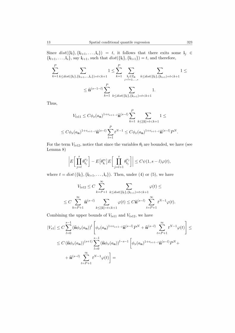
13 Spatial conditional quantile regression 323
Since dist(il, il+1, . . . , is) = t, it follows that there exits some ij ∈il+1, . . . , is, say il+1, such that dist(il, il+1) = t, and therefore,
P∑k=1
∑k≤dist(il,il+1,...,is)=t<k+1
1 ≤P∑
k=1
∑ij∈In
j=l+2,...,s
∑k≤dist(il,il+1)=t<k+1
1 ≤
≤ n(s−1−l)P∑
k=1
∑k≤dist(il,il+1)=t<k+1
1.
Thus,
Vls11 ≤ Cφx(an)1+vs+1−ln(s−l)P∑
k=1
∑k≤‖i‖=t<k+1
1 ≤
≤ Cφx(an)1+vs+1−ln(s−l)P∑
t=1
tN−1 ≤ Cφx(an)1+vs+1−ln(s−l)PN .
For the term Vls12, notice that since the variables θi are bounded, we have (seeLemma 8) ∣∣∣∣E[ s∏
j=l
θνj
ij
]− E
[θνlil
]E
[ s∏j=l+1
θνj
ij
]∣∣∣∣ ≤ Cψ(1, s− l)ϕ(t),
where t = dist (il, il+1, . . . , is). Then, under (4) or (5), we have
Vls12 ≤ C∞∑
k=P+1
∑k≤dist(il,il+1)=t<k+1
ϕ(t) ≤
≤ C
∞∑k=P+1
n(s−l)∑
k≤‖i‖=t<k+1
ϕ(t) ≤ Cn(s−l)∞∑
t=P+1
tN−1ϕ(t).
Combining the upper bounds of Vls11 and Vls12, we have
|Vs1| ≤ Cs−1∑l=0
(nφx(an))l
[φx(an)1+vs+1−ln(s−l)PN + n(s−l)
∞∑t=P+1
tN−1ϕ(t)
]≤
≤ C (nφx(an))(s+1)s−1∑l=0
(nφx(an))l−s−1
[φx(an)1+vs+1−ln(s−l)PN+
+ n(s−l)∞∑
t=P+1
tN−1ϕ(t)]
=

324 Sophie Dabo-Niang, Zoulikha Kaid and Ali Laksaci 14
= C (nφx(an))(s+1)s−1∑l=0
[n−1PNφx(an)1+vs+1−lφx(an)l−s−1+
+ n−1φx(an)(l−s−1)∞∑
t=P+1
tN−1ϕ(t)]≤
≤ C (nφx(an))(s+1)s−1∑l=0
[n−1PNφx(an)1+vs+1−lφx(an)l−s−1+
+ n−1φx(an)(l−s−1)P−sN∞∑
t=P+1
tsN+N−1ϕ(t)].
Taking P = φx(an)−1/N , we obtain
|Vs1| ≤ C (nφx(an))(s+1)s−1∑l=0
[1
nφx(an)φx(an)1+vs+1−lφx(an)l−s−1+
+1
nφx(an)(φx(an)l)
∞∑t=P+1
tsN+N−1−δ
]≤ C (nφx(an))(s+1)
since δ > N(p+ 2).
Proof of iii). As indicated in Gao et al. (2008), since the arguments aresimilar for any m ≤ s ≤ 2m − 1, the proof is given only for s = 2m − 1 andN = 2 for simplicity. In this case, V2m−1(ν0, ν1, . . . , ν2m−1) is denoted W . Tosimplify the notations, we write i = (i, j) ∈ Z2 and ik = (ik, jk) ∈ Z2. Themain difficulty is to cope with the summation∑
i0 6=i1 6=...i2m−1
E[θi0θi1 . . . θi2m−1
]=
=∑
(i0,j0) 6=(i1,j1) 6=···6=(i2m−1,j2m−1)
E[θi0j0θi1j1 . . . θi2m−1j2m−1
].
To this end, a novel ordering in Z2 (see Gao et al. (2008)), makes possibleto separate the indexes into two (or more) sets whose distance is greater orsmaller than P (usually larger than 1) is considered. Arrange each of theindex sets i0, i1, . . . , i2m−1 and j0, j1, . . . , j2m−1 in ascending orders as(retaining the same notation for the first ordered index set for simplicity)i0 ≤ i1 ≤ · · · ≤ i2m−1 and jl0 ≤ jl1 ≤ · · · ≤ jl2m−1 , where lk is to indicate thatlk may not be equal to k. The number of such arrangements is at most (2m)!.Let ∆ik = ik− ik−1 and ∆jk = jlk − jlk−1 and arrange ∆i1, . . . ,∆i2m−1 and∆j1, . . . ,∆j2m−1 in decreasing orders, respectively as ∆ia1 ≥ · · · ≥ ∆ia2m−1
and ∆jb1 ≥ · · · ≥ ∆jb2m−1 . Let t1 = ∆iam , t2 = ∆jbm and t = maxt1, t2. If

15 Spatial conditional quantile regression 325
t1 ≥ t2 then t = t1, and 0 ≤ iak− iak−1
≤ t1 ≤ n1 for k = m+ 1, . . . , 2m− 1,0 ≤ jlbk
− jlbk−1≤ t ≤ n2 for k = m,m+ 1, . . . , 2m− 1. Therefore,
(10) iak−1≤ iak
≤ iak−1+t, jlbk−1
≤ jbk≤ jlbk−1
+t for k = m+1, . . . , 2m−1.
We arrange i0 6= i1 6= · · · 6= i2m−1 according to the order of i0 ≤ i1 ≤ · · · ≤i2m−1. If t1 < t2, arrange according to the order of jl0 ≤ jl1 ≤ · · · ≤ jl2m−1 andthe proof is similar.
Let I = i1, . . . , i2m−1, Ia = ia1 , . . . , iam, Ica = I − Ia =
iam+1 , . . . , ia2m−1, J = jl1 , . . . , jl2m−1, Jb = jlb1 , . . . , jlbm and J c
b = J −Jb = jlbm+1
, . . . , jlb2m−1. Remark that (ia1 , . . . , ia2m−1) and (jlb1 , . . . , jlb2m−1
)are permutations of respectively I and J . Then, from (10), t = iam − iam−1
and t ≥ jlbm− jlbm−1
, we deduce that
W =∑
i0 6=i1 6=...i2m−1
E[θi0θi1 . . . θi2m−1
]≤ C
∑1≤i0≤i1≤···≤i2m−1≤n1
∑1≤jl0
≤jl1≤···≤jl2m−1
≤n2
∣∣E [θi0j0θi1j1 . . . θi2m−1j2m−1
]∣∣≤ C
max(n1,n2)∑t=1
n1∑i0=1
n1∑i=1
i∈Ia−iam
iak−1+t∑iak
=iak−1k=m+1,...,2m−1
n2∑jl0
=1
n2∑j=1
j∈Jb−jlbm
jlbk−1+t∑
jlbk=jlbk−1
k=m,m+1,...,2m−1
·
·∣∣E [θi0θi1 . . . θi2m−1
]∣∣ .Take a positive constant P such that 1 ≤ P ≤ max(n1, n2) and divide theright hand side of the previous inequality into two parts denoted by W1 andW2 according to 1 ≤ t ≤ P and t > P . Then, W ≤ W1 +W2. In one hand,use the result i) with s = 2m, and get
W1 = CP∑
t=1
n1∑i0=1
n1∑i=1
i∈Ia−iam
iak−1+t∑
iak=iak−1
k=m+1,...,2m−1
n2∑jl0
=1
n2∑j=1
j∈Jb−jlbm
jlbk−1+t∑
jlbk=jlbk−1
k=m,m+1,...,2m−1
·
·∣∣E [θi0θi1 . . . θi2m−1
]∣∣≤ C
P∑t=1
n1∑i0=1
n1∑i=1
i∈Ia−iam
iak−1+t∑
iak=iak−1
k=m+1,...,2m−1
n2∑jl0
=1
n2∑j=1
j∈Jb−jlbm
jlbk−1+t∑
jlbk=jlbk−1
k=m,m+1,...,2m−1
φx(an)1+v2m
≤ C(n1n2)mP∑
t=1
t2m−1φx(an)1+v2m ≤ C(n1n2)mP 2mφx(an)1+v2m .
326 Sophie Dabo-Niang, Zoulikha Kaid and Ali Laksaci 16
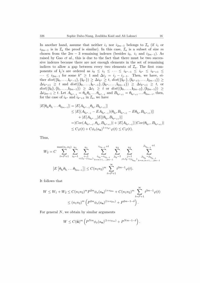
In another hand, assume that neither i1 nor i2m−1 belongs to Ia (if i1 ori2m−1 is in Ia the proof is similar). In this case, Ia is a subset of size mchosen from the 2m − 3 remaining indexes (besides i0, i1 and i2m−1). Asraised by Gao et al., this is due to the fact that there must be two succes-sive indexes because there are not enough elements in the set of remainingindices to allow a gap between every two elements of Ia. The first com-ponents of ij ’s are ordered as i0 ≤ i1 ≤ · · · ≤ ik∗−1 ≤ ik∗ ≤ ik∗+1 ≤· · · ≤ i2m−1 for some k∗ ≥ 1 and ∆ij = ij − ij−1. Then, we have, ei-ther dist(i0, . . . , ik∗−1, ik∗) ≥ ∆ik∗ ≥ t, dist(ik∗, ik∗+1, . . . , i2m−1) ≥∆ik∗+1 ≥ t and dist(i0, . . . , ik∗−1, ik∗ , . . . , i2m−1) ≥ ∆ik∗+1 ≥ t, ordist(i0, i1, . . . , i2m−1) ≥ ∆i1 ≥ t or dist(i0, . . . , i2m−2, i2m−1) ≥∆i2m−1 ≥ t. Let Aik∗−1
= θi0θi1 . . . θik∗−1and Bik∗+1
= θik∗+1. . . θi2m−1 , then,
for the case of ik∗ and ik∗+1 in Ia, we have
|E[θi0θi1 . . . θi2m−1 ]| = |E[Aik∗−1θik∗Bik∗+1
]|≤ |E[(Aik∗−1
− EAik∗−1)(θik∗Bik∗+1
− Eθik∗Bik∗+1)]|
+ |E[Aik∗−1]E[(θik∗Bik∗+1
)]|= |Cov(Aik∗−1
, θik∗Bik∗+1)|+ |E[Aik∗−1
]| |Cov(θik∗ , Bik∗+1)|
≤ Cϕ(t) + Cφx(an)1+vk∗ϕ(t) ≤ Cϕ(t).
Thus,
W2 = C
max(n1,n2)∑t=P+1
n1∑i0=1
n1∑i=1
i∈Ia−iam
iak−1+t∑
iak=iak−1
k=m+1,...,2m−1
n2∑jl0
=1
n2∑j=1
j∈Jb−jlbm
jlbk−1+t∑
jlbk=jlbk−1
k=m,m+1,...,2m−1∣∣E [θi0θi1 . . . θi2m−1
]∣∣ ≤ C(n1n2)m∞∑
t=P+1
t2m−1ϕ(t).
It follows that
W ≤W1 +W2 ≤ C(n1n2)mP 2mφx(an)1+v2m + C(n1n2)m∞∑
t=P+1
t2m−1ϕ(t)
≤ (n1n2)m(P 2mφx(an)(1+v2m) + P 2m−1−δ
).
For general N , we obtain by similar arguments
W ≤ C(n)m(PNmφx(an)(1+vNm) + PNm−1−δ
).

17 Spatial conditional quantile regression 327
Taking P = φx(an)−(1+vNm)/1+δ), we get
W ≤ C(nφx(an))m
(n−1φx(an)−Nm−1+(1+vNm)+(nφx(an))−1
∞∑t=P+1
tNm−1−δ
)≤ C(nφx(an))m
because δ > N(p+ 2). This ends the proof of the lemma.
Proof of Lemma 3. We have for all ε < 1,
P(F x
D = 0)≤ P
(F x
D ≤ 1− ε)≤ P
(|F x
D − E[F xD]| ≥ ε
).
Markov’s inequality allows to get, for any p > 0,
P(|F x
D − E[F xD]| ≥ ε
)≤E[|F x
D − E[F xD]|p
]εp
.
So, (P(F x
D = 0))1/p
= O(∥∥F x
D − E[F xD]∥∥
p
).
The computation of∥∥F x
D −E[F xD]∥∥
pcan be done by following the same argu-
ments as those used to prove Lemma 2. This yields the proof.
Proof of Lemma 4. Let us calculate the variance V ar(∆i). We have
V ar(∆i) =1
EK2i
[EK2
i (α−Hi(qα))2 − (EKi (α−Hi(qα)))2]
=1
EK2i
EK2i (α−Hi(qα))2 − (EKi)
2
EK2i
[EKi (Hi(qα)−α)
EKi
]2
= A1−A2.
Let us first consider A2. We deduce from the hypothesis H3 that thereexist two positive constants C and C ′ such that Cφx(an) ≤ EKr
i ≤ C ′φx(an),
r > 1, thus, (EKi)2
EK2i
= o(1). If we take the conditional expectation with respectto X, we get∣∣∣∣E[Ki(Hi(qα)−α)
EKi
]∣∣∣∣= ∣∣∣∣E Ki
EKi[E(Hi(qα)|X)−α]
∣∣∣∣≤E Ki
EKi|E(Hi(qα)|Xi)−α|.
It is easy to see that by hypothesis H ′4 (ii)
|E (Hi(qα)|X)− α| = |E (Hi(qα)|X)− F x(qα)|
≤ C
(ab1n + bb2n
∫R|t|b2
∣∣K(1)2 (t)
∣∣dt) ,∣∣∣∣EKi (Hi(qα)− α)
EKi
∣∣∣∣ = O(ab1n + bb2n
).

328 Sophie Dabo-Niang, Zoulikha Kaid and Ali Laksaci 18
Then, we deduce that A2 tends to 0. Concerning A1, we have
(α−Hi(qα))2 =(H2
i (qα)− α)− 2α (Hi(qα)− α) + α− α2.
Then, we can write
A1 =1
EK2i
[EK2
i
(H2
i (qα)− α)− 2αEK2
i (Hi(qα)− α)]+ α (1− α) .
The conditional expectation with respect to Xi, permits to obtain
A1 = EK2
i
EK2i
[E(H2
i (qα)|Xi
)− α
]−2αE
K2i
EK2i
[E (Hi(qα)|Xi)− α]+α (1− α) .
The same argument as above, gives∣∣∣∣E K2i
EK2i
[E (Hi(qα)|Xi)− α]∣∣∣∣ = O
(ab1n + bb2n
).
It remains to show that∣∣E (H2i (qα)|Xi
)− α
∣∣ = O(ab1n + bb2n
).
By an integration by part and hypotheses H ′2 and H ′
4, we have
∣∣E (H2i (qα)|Xi
)− α
∣∣ = ∣∣∣∣∫RK2
2
(qα − z
bn
)fXi(z)dz − F x(qα)
∣∣∣∣=∣∣∣∣∫
R2K2(t)K
(1)2 (t)
(FXi(qα − bnt)− F x(qα)
)dt∣∣∣∣
≤ ab1n
∫R
2K2(t)K(1)2 (t)dt+ bb2n
∫R
2K2(t)|t|b2K(1)2 (t)dt
≤ Cab1n + bb2n
∫R
2|t|b2K(1)2 (t)dt = O
(ab1n + bb2n
).
We deduce from above that A1 converges to α (1− α); then,
V ar (∆i) → α (1− α) .
Let us focus now on the covariance term. We consider
E1 = i, j ∈ In : 0 < ‖i− j‖ ≤ cn,
E2 = i, j ∈ In : ‖i− j‖ > cn.
19 Spatial conditional quantile regression 329
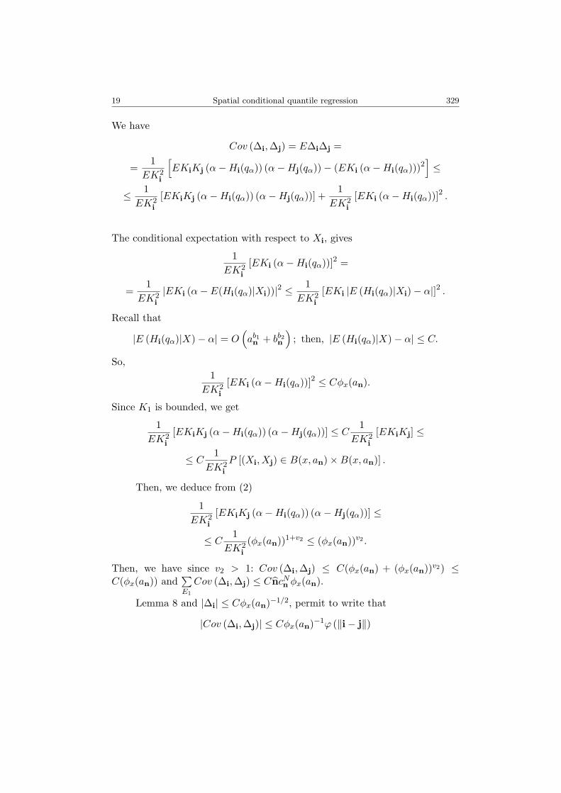
We have
Cov (∆i,∆j) = E∆i∆j =
=1
EK2i
[EKiKj (α−Hi(qα)) (α−Hj(qα))− (EKi (α−Hi(qα)))2
]≤
≤ 1EK2
i
[EKiKj (α−Hi(qα)) (α−Hj(qα))] +1
EK2i
[EKi (α−Hi(qα))]2 .
The conditional expectation with respect to Xi, gives
1EK2
i
[EKi (α−Hi(qα))]2 =
=1
EK2i
|EKi (α− E(Hi(qα)|Xi))|2 ≤1
EK2i
[EKi |E (Hi(qα)|Xi)− α|]2 .
Recall that
|E (Hi(qα)|X)− α| = O(ab1n + bb2n
); then, |E (Hi(qα)|X)− α| ≤ C.
So,1
EK2i
[EKi (α−Hi(qα))]2 ≤ Cφx(an).
Since K1 is bounded, we get
1EK2
i
[EKiKj (α−Hi(qα)) (α−Hj(qα))] ≤ C1
EK2i
[EKiKj] ≤
≤ C1
EK2i
P [(Xi, Xj) ∈ B(x, an)×B(x, an)] .
Then, we deduce from (2)
1EK2
i
[EKiKj (α−Hi(qα)) (α−Hj(qα))] ≤
≤ C1
EK2i
(φx(an))1+v2 ≤ (φx(an))v2 .
Then, we have since v2 > 1: Cov (∆i,∆j) ≤ C(φx(an) + (φx(an))v2) ≤C(φx(an)) and
∑E1
Cov (∆i,∆j) ≤ CncNn φx(an).
Lemma 8 and |∆i| ≤ Cφx(an)−1/2, permit to write that
|Cov (∆i,∆j)| ≤ Cφx(an)−1ϕ (‖i− j‖)

330 Sophie Dabo-Niang, Zoulikha Kaid and Ali Laksaci 20
and∑E2
Cov (∆i,∆j) ≤ Cφx(an)−1∑
(i,j)∈E2
ϕ (‖i− j‖) ≤ Cnφx(an)−1∑
i:‖i‖>cn
ϕ (‖i‖)
≤ Cnφx(an)−1c−δn
∑i:‖i‖>cn
‖i‖δϕ (‖i‖) .
Finally, for δ > 0 we have∑Cov (∆i,∆j) ≤
(CncNn φx(an) + Cnφx(an)−1c−δ
n
∑i:‖i‖>cn
‖i‖δϕ (‖i‖)).
Let cn = φx(an)−1/N , then, we have∑Cov (∆i,∆j) ≤
(Cn + Cnφx(an)δ/N−1
∑i:‖i‖>cn
‖i‖δϕ (‖i‖)).
Hence, we obtain that ∑Cov (∆i,∆j) = o (n) .
In conclusion, we have
1nvar
(∑i∈In
∆i
)=(var (∆i)+
1n
∑i,j∈In
Cov (∆i,∆j))→α(1−α) when n→∞.
This yields the proof.
Proof of Lemma 5. Let
Sn =nk∑
jk=1k=1,...,N
∆j
with
∆j =1√EKi
[αKi −KiHi(qα)− E (αKi −KiHi(qα))] .
Then, we can write[nE2Ki
α(1− α)EK2i
]1/2 ([αF x
D − F xN (qα)
]− E
[αF x
D − F xN (qα)
])=
= (nα(1− α))−1/2 Sn.
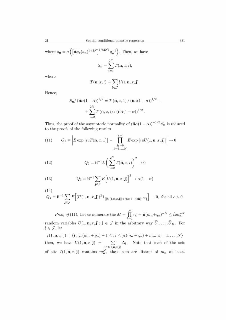
Consider the same spatial block decomposition (due to Tran (1990)) asLemma 2, with qn = o
([nφx(an)(1+2N)
]1/(2N)), mn =
[(nφx(an))1/(2N)/sn
]
21 Spatial conditional quantile regression 331
where sn = o([
nφx(an)1+2N]1/(2N)
q−1n
). Then, we have
Sn =2N∑i=1
T (n, x, i),
whereT (n, x, i) =
∑j∈J
U(i,n, x, j).
Hence,
Sn/ (nα(1− α))1/2 = T (n, x, 1) / (nα(1− α))1/2 +
+2N∑i=2
T (n, x, i) / (nα(1− α))1/2 .
Thus, the proof of the asymptotic normality of (nα(1− α))−1/2 Sn is reducedto the proofs of the following results
(11) Q1 ≡∣∣∣∣E exp
[iuT (n, x, 1)
]−
rk−1∏jk=0
k=1,...,N
E exp[iuU(1,n, x, j)
]∣∣∣∣→ 0
(12) Q2 ≡ n−1E
( 2N∑i=2
T (n, x, i))2
→ 0
(13) Q3 ≡ n−1∑j∈J
E[U(1,n, x, j)
]2→ α(1− α)
(14)Q4 ≡ n−1
∑j∈J
E[(U(1,n, x, j))21|U(1,n,x,j)|>ε(α(1−α)n)1/2
]→ 0, for all ε > 0.
Proof of (11). Let us numerate theM =N∏
k=1
rk = n(mn+qn)−N ≤ nm−Nn
random variables U(1,n, x, j); j ∈ J in the arbitrary way U1, . . . , UM . Forj ∈ J , let
I(1,n, x, j) = i : jk(mn + qn) + 1 ≤ ik ≤ jk(mn + qn) +mn; k = 1, . . . , N
then, we have U(1,n, x, j) =∑
i∈I(1,n,x,j)
∆i. Note that each of the sets
of site I(1,n, x, j) contains mNn , these sets are distant of mn at least.
332 Sophie Dabo-Niang, Zoulikha Kaid and Ali Laksaci 22
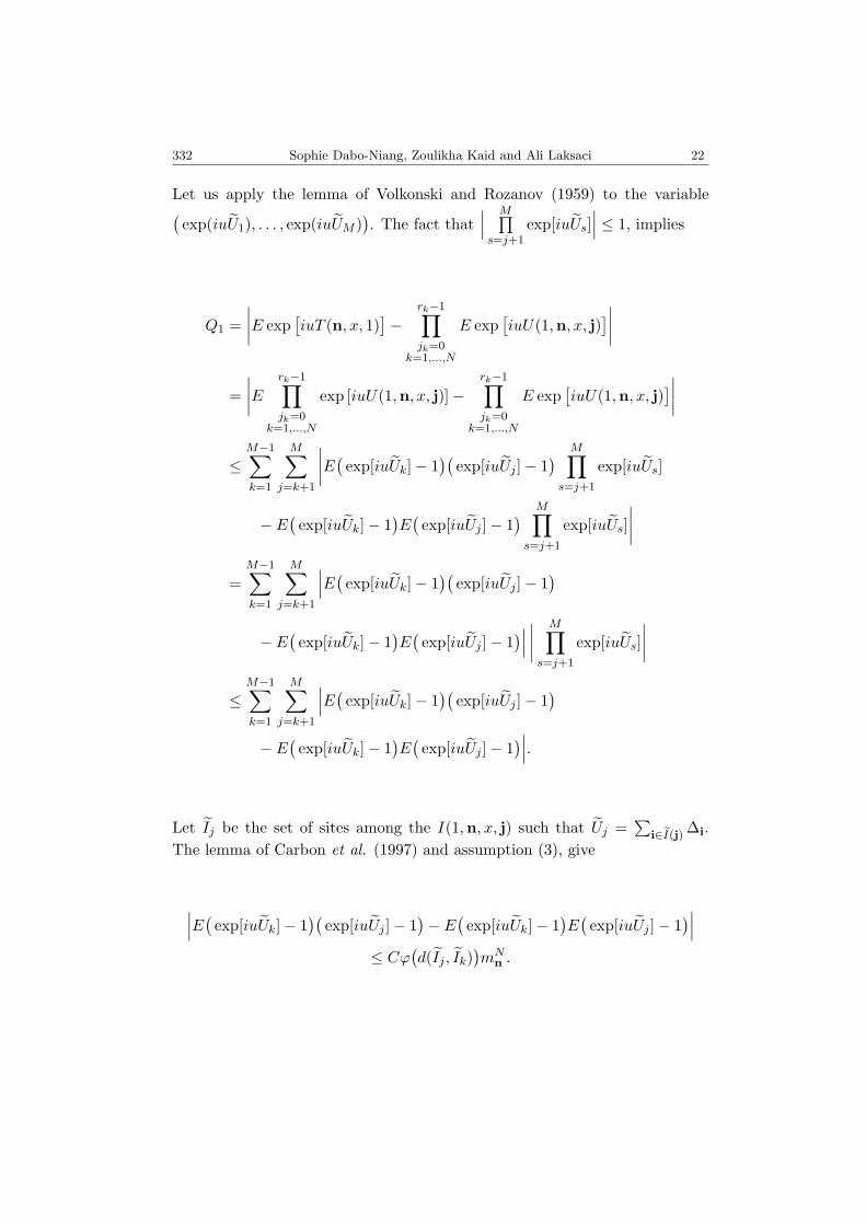
Let us apply the lemma of Volkonski and Rozanov (1959) to the variable(exp(iuU1), . . . , exp(iuUM )
). The fact that
∣∣∣ M∏s=j+1
exp[iuUs]∣∣∣ ≤ 1, implies
Q1 =∣∣∣∣E exp
[iuT (n, x, 1)
]−
rk−1∏jk=0
k=1,...,N
E exp[iuU(1,n, x, j)
]∣∣∣∣=∣∣∣∣E rk−1∏
jk=0k=1,...,N
exp [iuU(1,n, x, j)]−rk−1∏jk=0
k=1,...,N
E exp[iuU(1,n, x, j)
]∣∣∣∣≤
M−1∑k=1
M∑j=k+1
∣∣∣∣E( exp[iuUk]− 1)(
exp[iuUj ]− 1) M∏
s=j+1
exp[iuUs]
− E(exp[iuUk]− 1
)E(exp[iuUj ]− 1
) M∏s=j+1
exp[iuUs]∣∣∣∣
=M−1∑k=1
M∑j=k+1
∣∣∣E( exp[iuUk]− 1)(
exp[iuUj ]− 1)
− E(exp[iuUk]− 1
)E(exp[iuUj ]− 1
)∣∣∣ ∣∣∣∣ M∏s=j+1
exp[iuUs]∣∣∣∣
≤M−1∑k=1
M∑j=k+1
∣∣∣E( exp[iuUk]− 1)(
exp[iuUj ]− 1)
− E(exp[iuUk]− 1
)E(exp[iuUj ]− 1
)∣∣∣.
Let Ij be the set of sites among the I(1,n, x, j) such that Uj =∑
i∈I(j)∆i.
The lemma of Carbon et al. (1997) and assumption (3), give
∣∣∣E( exp[iuUk]− 1)(
exp[iuUj ]− 1)− E
(exp[iuUk]− 1
)E(exp[iuUj ]− 1
)∣∣∣≤ Cϕ
(d(Ij , Ik)
)mN
n .

23 Spatial conditional quantile regression 333
Then,
Q1 ≤ CmNn
M−1∑k=1
M∑j=k+1
ϕ(d(Ij , Ik)
)≤ CmN
n MM∑
k=2
ϕ(d(I1, Ik)
)≤ CmN
n M
∞∑i=1
∑k:iqn≤d(I1,Ik)<(i+1)qn
ϕ(d(I1, Ik)
)
≤ CmNn M
∞∑i=1
iN−1ϕ(iqn) ≤ Cnq−Nδn
∞∑i=1
iN−1−Nδ,
by (6). This last tends to zero by the fact that nq−Nδn → 0 (see (H5)).
Proof of (12). We have
Q2 ≡ n−1E
( 2N∑i=2
T (n, x, i))2
=
= n−1
( 2N∑i=2
E [T (n, x, i)]2 +∑
i,j=2,...,2N
i6=j
E [T (n, x, i)] [T (n, x, j)]).
By Cauchy-Schwartz inequality, we get ∀ 2 ≤ i ≤ 2N :
n−1E [T (n, x, i)] [T (n, x, j)] ≤(n−1E [T (n, x, i)]2
)1/2(n−1E [T (n, x, j)]2
)1/2.
Then, it suffices to prove that
n−1E [T (n, x, i)]2 → 0, ∀ 2 ≤ i ≤ 2N .
We will prove this for i = 2, the case where i 6= 2 is similar. We have
T (n, x, 2) =∑j∈J
U(2,n, x, j) =M∑
j=1Uj , where we enumerate the U(2,n, x, j)
in the arbitrary way U1, . . . , UM . Then,
E [T (n, x, 2)]2 =M∑i=1
V ar(Ui
)+
M∑i=1
M∑j=1i6=j
Cov(Ui, Uj
)= A1 +A2.

334 Sophie Dabo-Niang, Zoulikha Kaid and Ali Laksaci 24
The stationarity of the process (Xi, Yi)i∈ZN , implies that
V ar(Ui) = V ar
( mn∑ik=1
k=1,...,N−1
qn∑iN=1
∆i
)2
= mN−1n qn V ar (∆i) +
mn∑ik=1
k=1,...,N−1
qn∑iN=1
mn∑jk=1
k=1,...,N−1i 6=j
qn∑jN=1
E∆i∆j.
We proved above that V ar (∆i) < C. By Lemma 8, we have
(15) |E∆i(x)∆j(x)| ≤ Cφx(an)−1ϕ (‖i− j‖) .
Then, we deduce that
V ar(Ui) ≤ CmN−1n qn
(1 + φx(an)−1
mn∑ik=1
k=1,...,N−1
qn∑iN=1
(ϕ (‖i‖)))
≤ CmN−1n qnφx(an)−1
mn∑ik=1
k=1,...,N−1
qn∑iN=1
(ϕ(‖i‖) .
Consequently, we have
A1 ≤ CMmN−1n qnφx(an)−1
∞∑i=1
iN−1 (ϕ(i)) .
Let
I (2,n, x, j) =i : jk(mn + qn) + 1 ≤ ik ≤ jk(mn + qn) +mn, 1 ≤ k ≤ N − 1;
+jN (mn + qn) +mn + 1 ≤ iN ≤ (JN + 1)(mn + qn).
The variable U (2,n, x, j) is the sum of the ∆i such that i is in I (2,n, x, j).Since mn > qn, if i and i′ are respectively in the two different sets I (2,n, x, j)and I (2,n, x, j′); then, ik 6= i′k, for a certain k such that 1 ≤ k ≤ N and‖i− i′‖ > qn.
By using the definition of A2, the stationarity of the process and (15),we have
A2 ≤
nk∑jk=1
k=1,...,N
nk∑ik=1
k=1,...,N‖i−j‖>qn
E∆i∆j ≤ Cφx(an)−1nnk∑
ik=1k=1,...,N‖i‖>qn
(ϕ(‖i‖))
25 Spatial conditional quantile regression 335
and
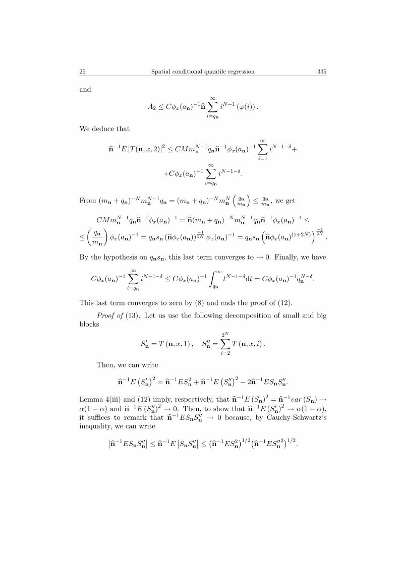
A2 ≤ Cφx(an)−1n∞∑
i=qn
iN−1 (ϕ(i)) .
We deduce that
n−1E [T (n, x, 2)]2 ≤ CMmN−1n qnn−1φx(an)−1
∞∑i=1
iN−1−δ+
+Cφx(an)−1∞∑
i=qn
iN−1−δ.
From (mn + qn)−NmN−1n qn = (mn + qn)−NmN
n
(qnmn
)≤ qn
mn, we get
CMmN−1n qnn−1φx(an)−1 = n(mn + qn)−NmN−1
n qnn−1φx(an)−1 ≤
≤(qnmn
)φx(an)−1 = qnsn (nφx(an))
−12N φx(an)−1 = qnsn
(nφx(an)(1+2N)
)−12N.
By the hypothesis on qnsn, this last term converges to → 0. Finally, we have
Cφx(an)−1∞∑
i=qn
iN−1−δ ≤ Cφx(an)−1
∫ ∞
qn
tN−1−δdt = Cφx(an)−1qN−δn .
This last term converges to zero by (8) and ends the proof of (12).
Proof of (13). Let us use the following decomposition of small and bigblocks
S′n = T (n, x, 1) , S′′n =2N∑i=2
T (n, x, i) .
Then, we can write
n−1E(S′n)2 = n−1ES2
n + n−1E(S′′n)2 − 2n−1ESnS
′′n.
Lemma 4(iii) and (12) imply, respectively, that n−1E (Sn)2 = n−1var (Sn) →α(1 − α) and n−1E (S′′n)2 → 0. Then, to show that n−1E (S′n)2 → α(1 − α),it suffices to remark that n−1ESnS
′′n → 0 because, by Cauchy-Schwartz’s
inequality, we can write∣∣n−1ESnS′′n
∣∣ ≤ n−1E∣∣SnS
′′n
∣∣ ≤ (n−1ES2n
)1/2(n−1ES′′n2)1/2
.
336 Sophie Dabo-Niang, Zoulikha Kaid and Ali Laksaci 26
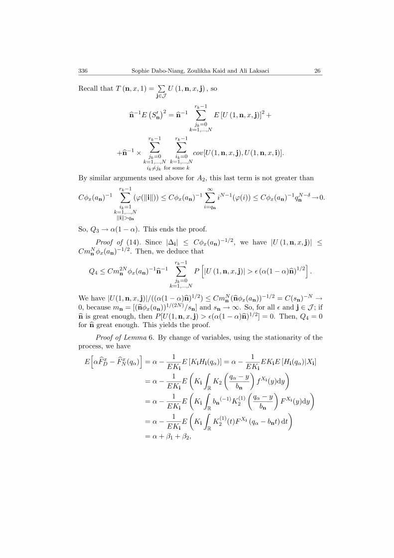
Recall that T (n, x, 1) =∑j∈J
U (1,n, x, j) , so
n−1E(S′n)2 = n−1
rk−1∑jk=0
k=1,...,N
E [U (1,n, x, j)]2 +
+n−1 ×
rk−1∑jk=0
k=1,...,N
rk−1∑ik=0
k=1,...,Nik 6=jk for some k
cov[U(1,n, x, j), U(1,n, x, i)].
By similar arguments used above for A2, this last term is not greater than
Cφx(an)−1rk−1∑ik=1
k=1,...,N‖i‖>qn
(ϕ(‖i‖)) ≤ Cφx(an)−1∞∑
i=qn
iN−1(ϕ(i)) ≤ Cφx(an)−1qN−δn →0.
So, Q3 → α(1− α). This ends the proof.
Proof of (14). Since |∆i| ≤ Cφx(an)−1/2, we have |U (1,n, x, j)| ≤CmN
n φx(an)−1/2. Then, we deduce that
Q4 ≤ Cm2Nn φx(an)−1n−1
rk−1∑jk=0
k=1,...,N
P[|U (1,n, x, j)| > ε (α(1− α)n)1/2
].
We have |U(1,n, x, j)|/((α(1− α)n)1/2) ≤ CmNn (nφx(an))−1/2 = C(sn)−N →
0, because mn = [(nφx(an))1/(2N)/sn] and sn →∞. So, for all ε and j ∈ J ; ifn is great enough, then P [U(1,n, x, j) > ε(α(1− α)n)1/2] = 0. Then, Q4 = 0for n great enough. This yields the proof.
Proof of Lemma 6. By change of variables, using the stationarity of theprocess, we have
E[αF x
D − F xN (qα)
]= α− 1
EKiE [KiHi(qα)] = α− 1
EKiEKiE [Hi(qα)|Xi]
= α− 1EKi
E
(Ki
∫RK2
(qα − y
bn
)fXi(y)dy
)= α− 1
EKiE
(Ki
∫Rbn
(−1)K(1)2
(qα − y
bn
)FXi(y)dy
)= α− 1
EKiE
(Ki
∫RK
(1)2 (t)FXi (qα − bnt) dt
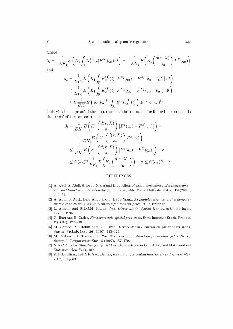
)= α+ β1 + β2,
27 Spatial conditional quantile regression 337
where
β1 =− 1EKi
E
(Ki
∫RK
(1)2 (t)FXi(qα)dt
)= − 1
EKiE
(K1
(d(x,X)an
)FX(qα)
)and
β2 =1
EKiE
(Ki
∫RK
(1)2 (t)
[FXi(qα)− FXi (qα − bnt)
]dt)
≤ 1EKi
E
(Ki
∫RK
(1)2 (t)
∣∣FXi(qα)− FXi (qα − bnt)∣∣ dt)
≤ C1
EKiE
(Ki(bn)b2
∫R|t|b2K(1)
2 (t))
dt ≤ C(bn)b2 .
This yields the proof of the first result of the lemma. The following result endsthe proof of the second result
β1 =1
EKiE
(K1
(d(x,X)an
)[F x(qα)− FX(qα)
])−
− 1EKi
E
(K1
(d(x,X)an
)F x(qα)
)≤ 1EKi
E
(K1
(d(x,X)an
) ∣∣F x(qα)− FX(qα)∣∣)− α
≤ C(an)b1 1EKi
E
(K1
(d(x,X)an
))− α ≤ C(an)b1 − α.
REFERENCES
[1] A. Abdi, S. Abdi, S. Dabo-Niang and Diop Aliou, P -mean consistency of a nonparamet-
ric conditional quantile estimator for random fields. Math. Methods Statist. 19 (2010),
1, 1–21.
[2] A. Abdi, S. Abdi, Diop Aliou and S. Dabo-Niang, Asymptotic normality of a nonpara-
metric conditional quantile estimator for random fields. 2010, Preprint.
[3] L. Anselin and R.J.G.M. Florax, New Directions in Spatial Econometrics. Springer,
Berlin, 1995.
[4] G. Biau and B. Cadre, Nonparametric spatial prediction. Stat. Inference Stoch. Process.
7 (2004), 327–349.
[5] M. Carbon, M. Hallin and L.T. Tran, Kernel density estimation for random fields.
Statist. Probab. Lett. 36 (1996), 115–125.
[6] M. Carbon, L.T. Tran and B. Wu, Kernel density estimation for random fields: the L1
theory. J. Nonparametr Stat. 6 (1997), 157–170.
[7] N.A.C. Cressie, Statistics for spatial Data. Wiley Series in Probability and Mathematical
Statistics, New York, 1991.
[8] S. Dabo-Niang and A.F. Yao, Density estimation for spatial functional random variables.
2007, Preprint.

338 Sophie Dabo-Niang, Zoulikha Kaid and Ali Laksaci 28
[9] S. Dabo-Niang and N. Rhomari. Estimation non parametrique de la regression avec
variable explicative dans un espace metrique. C.R. Acad. Sci. Paris Ser. I 336 (2003),
75–80.
[10] S. Dabo-Niang and A. Laksaci, Nonparametric estimation of conditional quantiles when
the regressor is valued in a semi-metric space. 2007, submitted.
[11] S. Dabo-Niang and A. Laksaci, Nonparametric quantile regression estimation for func-
tional dependent data. Math. Methods Statist., 2011, To appear.
[12] S. Dabo-Niang et B. Thiam, L1 consistency of a kernel estimate of spatial conditional
quantile. Statist. Probab. Lett. 80 (2010), 17–18, 1447–1458.
[13] F. Ferraty and Ph. Vieu, Nonparametric Functional Data Analysis. Springer-Verlag,
New York, 2006.
[14] X. Guyon, Estimation d’un champ par pseudo-vraisemblance conditionnelle: Etude
asymptotique et application au cas Markovien. Proceedings of the Sixth Franco-Belgian
Meeting of Statisticia, 1987.
[15] X. Guyon, Random Fields on a Network – Modeling, Statistics, and Applications.
Springer, New York, 1995.
[16] M. Hallin, Z. Lu and L.T. Tran, Kernel density estimation for spatial processes: the L1
theory. J. Multivariate Anal. 88 (2004), 1, 61–75.
[17] M. Hallin, Z. Lu and L.T. Tran, Local linear spatial regression. Ann. Statatist. 32 (2004),
6, 2469–2500.
[18] M. Hallin, Z. Lu and K. Yu, Local linear spatial quantile regression. Bernoulli 15 (2009),
3, 659–686.
[19] T. Honda, Nonparametric estimation of a conditional quantile for a mixing processes.
Ann. Inst. Statist. Math. 52 (2000), 459–470.
[20] R. Koenker, Galton, Edgrworth, Frish and prospect for quantile regression in economet-
rics. J. Econometrics 95 (2000), 347–374.
[21] R. Koenker, Quantile Regression, Cambridge University Press in econometrics. Cam-
bridge, U.K., 2005.
[22] R. Koenker and I. Mizera, Penalized triograms: total variation regularization for bivari-
ate smoothing. J. Roy. Statist. Soc. Ser. B 66 (2004), 145–164.
[23] H.L. Koul and K. Mukherjee, Regression quantiles and related processes under long
range dependence. J. Multivariate Anal. 51 (1994), 318–337.
[24] A. Laksaci and F. Maref, Estimation non parametrique de quantiles conditionnels pour
des variables fonctionnelles spatialement dependantes. C.R. Acad. Sci. Paris Ser. I Math.
347 (2009), 1075–1080.
[25] Z. Lu and X. Chen, Spatial nonparametric regression estimation: Non-isotropic Case
Acta Math. Appl. Sin. 18 (2002), 4, 641–656.
[26] Z. Lu and X. Chen, Spatial kernel regression estimation: weak concistency. Statist.
Probab. Lett. 68 (2004), 125–136.
[27] S.L. Portnoy, Asymptotic behavior of regression quantiles in nonstationary dependent
cases. J. Multivariate Anal. 38 (1991), 100–113.
[28] C. Preda, Regression models for functional data by reproducing kernel Hilbert spaces
methods. J. Statist. Plann. Inference 137 (2007), 829–840.
[29] B. Ripley, Spatial Statistics. Wiley, New York, 1981.

29 Spatial conditional quantile regression 339
[30] L.T. Tran, Kernel density estimation on random fields. J. Multivariate Anal. 34 (1990),
37–53.
[31] L.T. Tran and S. Yakowitz, Nearest neighbor estimators for random fields. J. Multivari-
ate Anal. 44 (1993), 23–46.
Received 14 April 2011 Universite Lille 3
Labo. EQUIPPE, Maison de la Recherche
BP 60149
59653 Villeneuve d’Ascq Cedex, France
Universite Djillali Liabes
Laboratoire de Statistique et Processus Stochastiques
BP 89, 22000 Sidi Bel Abbes, Algeria