Spatial Analysis of Solar Potential in Canberra Prepared for the Australian PV Institute by Jessie Copper, Mike Roberts and Anna Bruce, UNSW Sydney - November 2017

Summary

There is significant potential for rooftop solar PV in Australia. Rooftop solar PV is a key energy technology because it is leading the transition to consumer uptake of low-carbon demand-side energy technologies, which are providing new opportunities for consumer engagement and new clean energy business models to emerge. However, there is a lack of good information in the public domain about the potential for rooftop solar to contribute to low-carbon electricity generation in Australia’s cities. This type of information is important for policymakers and planners, and to encourage public support for rooftop solar.

This research uses the data and methodologies behind the APVI Solar Potential Tool http://pv-map.apvi.org.au/potential, developed by researchers at UNSW, to estimate the Solar Potential in the Canberra CBD. The report includes:

1. An assessment of PV Potential in Canberra CBD 2. An estimate of the potential impact of rooftop PV on local electricity consumption and emissions 3. Identification of rooftops with the largest PV potential (area available) in the CBD 4. Three case studies of PV Potential on landmark buildings in Canberra

The useable area suitable for PV deployment across Canberra’s CBD was calculated using two different methods. The most conservative estimate of the two suggests the useable area suitable for rooftop PV deployment (the ratio between the area of PV panels that could be accommodated and the total roof area) is 34% corresponding to 46 MW of PV potential with an expected annual yield of 67.6 GWh. The equivalent CO2 emission savings are 53 kt per year.

The average of the two methods indicated that an area equal to 50% of the available roof surfaces could be used to accommodate PV, corresponding to 68 MW of potential PV capacity with an expected annual yield of 98 GWh. This equates to 17% of the 560 GWh of load seen by all of the zone substations within or near the CBD area (560 GWh is an overestimate of the CBD load, since these substations also serve loads outside of the CBD area). This average figure of 98GWh is equivalent to the average load of 13,000 ACT households. The potential CO2-equivalent emission savings from PV based on the average of the two PV potential estimation methods are 77 kt per year. There is an estimated 1.3MW of existing PV capacity installed on Canberra CBD rooftops, approximately 2% of the potential capacity. Almost all of the electricity generation and emissions savings calculated would therefore be additional.

The rooftops with the largest PV potential in Canberra have been mapped (Figure 1 below). More detailed images appear in Appendix C.

large - med - small Figure 1: Rooftops with Largest PV Potential in Canberra CBD

Case studies of specific landmark buildings including the ACT Legislative Assembly, the Australian War Memorial and the Canberra Convention Centre have been conducted.

Table 1 shows the potential roof area available for PV installation on each building, based on the data and visual imagery available.

Table 1: Available roof areas on the Case Study Buildings

Site Building

Footprint (m2)

Total Roof Area (m2)

Developable Planes (m2)

Array Area (m2)

Array Area / Roof Area

ACT Legislative Assembly 3,247 2,615 2,346 1,664 64%

Australian War Memorial 15,572 13,343 10,813 7,682 58%

Canberra Convention Centre 10,160 10,160 7,762 4,554 45%

Table 2 shows the projected array capacity and expected annual energy production. The proposed PV arrays are illustrated in Figure 22 -Figure 24 below.

Table 2: Expected Annual Energy Production

Site

PV Capacity Annual Energy

Production (w/o shading)

Average Yield per kW PV installed

Expected Annual Energy

Production (adjusted)

(kWpeak) (MWh/year) (kWh/kW/day) (MWh/year) ACT Legislative Assembly 260 360 3.78 360

Australian War Memorial 1200 1682 3.84 1653 Canberra Convention Centre 712 1005 3.87 981

Table 3 presents the estimated carbon offsets for each system and shows that these three buildings could save an estimated 2.4 kilotonnes of carbon emissions each year and could supply the equivalent of 400 households, based on the average 2014 electricity demand of a Queensland household being 7470 kWh [1].

Table 3: Carbon offset and household energy equivalents

Site Expected Annual

Energy Production Emissions Offset Average ACT household

equivalent (MWh/year) (Tonnes CO2-e / year)

ACT Legislative Assembly 360 283 48 Australian War Memorial 1653 1298 221 Canberra Convention Centre 981 770 131

Totals 2995 2351 401

Array Illustrations

Figure 2: Potential PV Array on the ACT Legislative Assembly

Figure 3: Potential PV Array on the Australian War Memorial

Figure 4: Potential PV Array on Canberra Convention Centre

Introduction to the Solar Potential Tool

The APVI Solar Potential Tool (SPT) is an online tool to allow electricity consumers, solar businesses, planners and policymakers to estimate the potential for electricity generation from PV on building roofs. The tool accounts for solar radiation and weather at the site; PV system area, tilt, orientation; and shading from nearby buildings and vegetation.

The data behind the APVI SPT were generated as follows:

1. Three types of digital surfaces models (DSMs)1 (3D building models, XYZ vegetation points and 1m ESRI Grids), supplied by geospatial company AAM, were used to model the buildings and vegetation in the areas covered by the map.

2. These DSMs were used as input to ESRI’s ArcGIS tool to evaluate surface tilt, orientation and the annual and monthly levels of solar insolation falling on each 1m2 unit of surface.

3. Insolation values output by the ArcGIS model were calibrated2 to Typical Meteorological Year (TMY) weather files for each of the capital cities and against estimates of insolation at every 1 degree tilt and orientation from NREL’s System Advisor Model (SAM).

At a city level, an insolation heatmap layer (Figure 5b) allows identification of the best roofs, while the shadow layer (Figure 5c) allows the user to locate an unshaded area on a rooftop. On a specific roof surface, an estimate of annual electricity generation, financial savings and emissions offset from installing solar PV can be obtained.

Figure 5: (a) Aerial photograph (b) Insolation heat map, (c) Winter shadow layer

This project expanded the data and methodologies behind the Solar Potential in order to estimate the Solar Potential in the Canberra CBD region.

1 Digital surface models provide information about the earth’s surface and the height of objects. 3D building models and vegetation surface models have been used in this work. The ESRI Grid is a GIS raster file format developed by ESRI, used to define geographic grid space. 2 Calibration was required in order to obtain good agreement NREL’s well-tested SAM model and measured PV data.

Assessment of the PV Potential in Canberra CBD

This section of the report details the methodology and the results of the geospatial analysis of PV potential across Canberra CBD.

Methodology

The assessment of the PV potential in Canberra’s CBD, expanded on the initial work undertaken for the Canberra region of APVI’s SPT. The analysis made use of the following data sources:

1. The three sources of input DSMs data from AAM; and 2. City of Canberra LiDAR data – 2015 dataset sourced from the Geoscience Australia’s

Elevation Information System (ELVIS)

The general steps in the methodology are illustrated in Figure 6. To test the sensitivity of the estimated PV potential two input data sources and two rooftop suitability methods were assessed. The two input data sources used to calculate the tilt, aspect, solar insolation and determine suitable roof planes were 1) the DSM and 3D building models from AAM and 2) the 2015 Goescience Australia LiDAR data covering Canberra CBD. The two methods utilised to determine suitable rooftops were 1) based on a minimal level of surface insolation and 2) NREL’s PV rooftop suitability method based on hillshade and surface orientation. Both methods also required a minimum contiguous surface area of 10m2 for a roof plane to be determined suitable. This limit was defined to ensure a minimum 1.5kW PV system for any plane defined as suitable.

Figure 6: Major process steps for the calculation of rooftop PV potential

Input Data Source: AAM or LiDAR

Calculation of roof surface Tilt and Aspect Calculation of Hillshades

Calculation of surface Insolation

Identification of Unique roof surfaces

Assessment of rooftop suitability:

a) Insolation b) NREL Hillshade & aspect

Minimum criteria of 10m2 of contigous area

Calculation of PV Capacity and Yield per suitable roof

plane

Region aggregation to Sydney City Suburbs

Assessment of Rooftop Suitability - Methods

Method 1: Insolation Limit

The first method utilised to determine suitable roof planes was based on a minimum level of insolation. The minimum value was set at an annual average insolation of 3.93 kWh/m2/day. This limit was calculated as 80% of the expected level of annual insolation for a horizontal surface in Canberra, calculated as 4.91 kWh/m2/day, using the default TMY weather file for Canberra contained within the National Renewable Energy Laboratories (NREL) System Advisor Model (SAM). This limit was applied to the Solar Insolation Heat Map which was developed and calibrated as part of the APVI SPT methodology [2, 3].

Figure 8 presents an example application of the insolation limit in practice, displaying an aerial image (left), the insolation heat map (centre) and the classified insolation layer (right); classified as either above (white) or below (black) the insolation limit. As for each method in this report, a 10m2 contiguous area was required for a roof plane to be determined suitable. Figure 9 presents the roof planes that were identified to meet both the insolation and 10m2 contiguous area criteria for the example presented in Figure 8.

Figure 7 - Minimum distance from rooftop obstruction for 80% annual output

Figure 8: Example application of the Insolation limit. Areal image (left); Insolation heat map

(centre); and classified Insolation layer (right)

Figure 9: Example application of suitable planes (hatched areas) by the Insolation limit method.

Method 2: NREL’s Hillshade and Orientation

The second method utilised to determine suitable roof planes was the method developed by NREL to assess the technical potential for rooftop PV in the United States [4]. NREL’s method makes use of ArcGIS’s hillshade function to determine the number of hours of sunlight received on each 1m2 of roof surface, across 4 representative days within a year i.e. the winter and summer solstices and the two equinoxes; similar to the shadow layers of APVI’s SPT as illustrated in Figure 5.

To determine which areas met the shading criteria, NREL’s method defines that roof surfaces must meet a minimum number of hours of sunlight. The limit for any location can be determined by calculating the number of hours a rooftop would need to be in sunlight to produce 80% of the energy produced by an unshaded system of the same orientation [4]. For the location of Canberra the value was determined to be 14.04 hours across the 4 representative days.

In addition to the hillshade limit, NREL’s method also excludes roof planes based on orientation. In NREL’s method all roof planes facing northwest through northeast (i.e. 292.5 - 67.5 degrees for northern hemisphere locations) were considered unsuitable for PV. For southern hemisphere locations the equivalent exclusion would be orientations southeast through southwest (i.e. 112.5 – 247.5 degrees) as per Figure 10. Again, as for each method in this report, a 10m2 contiguous area is also required by NREL’s methodology.

Figure 10: Rooftop azimuths included in final suitable planes for the Southern Hemisphere

Figure 11 presents an example application of NREL’s hillshade and orientation limit in practice. For this particular example there is reasonable agreement between the surfaces determined as suitable for PV deployment from the two methods i.e. Figure 9 vs Figure 11. This is not always the case as evident in the example presented in Figure 12, which illustrates how the insolation limit method can define roof planes orientated southeast through southwest as suitable planes if the annual insolation meets the limit requirement.

Figure 11: Example application of the hillshade limit (left) with the suitable planes overlayed (right)

Figure 12: Comparison between roof planes defined as suitable by the insolation method (both - yellow) and NREL’s hillshade and orientation method (Left – orange)

Input Data Source: AAM 3D Building Model vs. LiDAR data

The other variable that affected the sensitivity of the estimated PV potential was the input data source. Two input data sources were available for use in this analysis:

1. The DSMs and 3D building models from AAM, which were utilised to generate the APVI SPT, 2. City of Canberra LiDAR data – 2015 dataset sourced from the Geoscience Australia’s

Elevation Information System (ELVIS).

The application of the PV potential analysis was applied identically to both input data sources.

Generally, Figure 13 demonstrates that there is general agreement between the roof planes identified as suitable via the two input data sources. However, the figure also illustrates how the analyses undertaken with the LiDAR data set excludes a greater proportion of roof surfaces.

Figure 13: Example of good agreement between the two input data source for large buildings. Aerial image (Left), AAM 3D buildings with Insolation limit method (centre); Canberra LiDAR with

Insolation limit method (Right)

Calculation of PV Capacity, Annual Yield and CO2-e Emission Reductions

After suitable roof planes have been identified, the PV capacity and annual yield for each roof surface can be calculated. The DC PV capacity (otherwise known as system size) was calculated as per APVI’s SPT methodology [2] using the DC size factor and array spacing methodologies [5]. The relevant equations for this method can be found here.

Generally, the method assumes a fixed DC size factor of 156.25 W/m2 (i.e. a 250W module with dimensions of 1m x 1.6m) for flush mounted arrays, and a variable DC size factor for rack mounted PV arrays. For rack mounted arrays, the DC size factor is a function of the PV array tilt and orientation and the tilt and orientation of the underlying roof surface. Figure 14 presents the equivalent useable roof area, which is analogous to the DC size factor, for a 15 degree tilted north facing PV array in Canberra, as a function of the tilt and orientation of the underlying roof surface. For an absolutely flat roof, Figure 14 indicates a useable area of 69%, analogous to a DC size factor of 108 W/m2. In comparison, NREL’s method assumes a fixed ratio of module to roof area of 70% for flat roof surfaces.

As per NREL’s method to calculate the PV potential in the United States [4], this analysis has assumed that rack mounted arrays will be installed on flat and relatively flat roof surfaces. For consistency with NREL’s method, flat roofs have been defined as roof surfaces with a tilt <= 9.5 degrees and the tilt angle of the rack mounted arrays were defined as 15 degrees.

Similarly, for tilted roof surfaces > 9.5 degrees, an additional module to roof area ratio of 0.98 was assumed in the NREL method to reflect 1.27cm of spacing between each module for racking clamps. This assumption was also applied in this study.

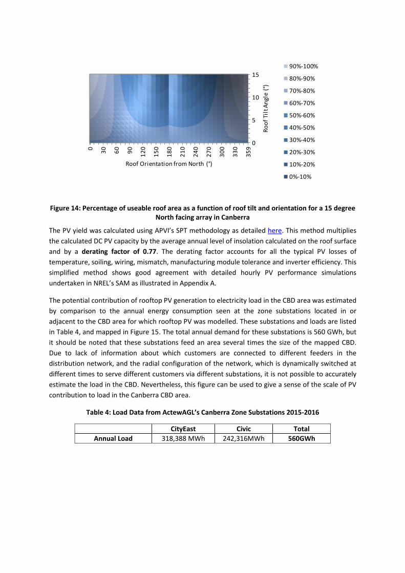
Figure 14: Percentage of useable roof area as a function of roof tilt and orientation for a 15 degree North facing array in Canberra

The PV yield was calculated using APVI’s SPT methodology as detailed here. This method multiplies the calculated DC PV capacity by the average annual level of insolation calculated on the roof surface and by a derating factor of 0.77. The derating factor accounts for all the typical PV losses of temperature, soiling, wiring, mismatch, manufacturing module tolerance and inverter efficiency. This simplified method shows good agreement with detailed hourly PV performance simulations undertaken in NREL’s SAM as illustrated in Appendix A.

The potential contribution of rooftop PV generation to electricity load in the CBD area was estimated by comparison to the annual energy consumption seen at the zone substations located in or adjacent to the CBD area for which rooftop PV was modelled. These substations and loads are listed in Table 4, and mapped in Figure 15. The total annual demand for these substations is 560 GWh, but it should be noted that these substations feed an area several times the size of the mapped CBD. Due to lack of information about which customers are connected to different feeders in the distribution network, and the radial configuration of the network, which is dynamically switched at different times to serve different customers via different substations, it is not possible to accurately estimate the load in the CBD. Nevertheless, this figure can be used to give a sense of the scale of PV contribution to load in the Canberra CBD area.

Table 4: Load Data from ActewAGL’s Canberra Zone Substations 2015-2016

0

5

10

15

0 30 60 90 120

150

180

210

240

270

300

330

359

Roof

Tilt

Ang

le (°

)

Roof Orientation from North (°)

90%-100%

80%-90%

70%-80%

60%-70%

50%-60%

40%-50%

30%-40%

20%-30%

10%-20%

0%-10%

CityEast Civic Total Annual Load 318,388 MWh 242,316MWh 560GWh

Figure 15 ActewAGL CBD Zone Substations [6] In order to assess the potential for additional rooftop PV in the Canberra CBD, and associated emissions reductions and electricity savings, existing PV capacity in the area was estimated. The CBD area covered by this assessment falls within the postcode areas 2601 and 2612 (see Figure 16 ). Using the Clean Energy Regulator’s database of PV systems registered under the Renewable Energy Target scheme (accessed via the APVI’s Solar Map[7]), which is a near complete record of PV systems installed in Australia, the installed PV capacity in these postcodes is listed in Table 5. It was assumed that 90% of the PV systems in 2601 and 50% of the PV systems in 2612 are installed on buildings within the CBD study area. The total existing PV capacity is therefore estimated to be around 1.3 MW.

Figure 16 Canberra CBD Postcode Areas

Table 5: Existing PV Capacity in Canberra CBD Postcodes

POA Total PV Capacity

(kW)

PV less than 10kW

(kW)

PV 10kW to 100kW

(kW)

PV bigger than 100kW

(kW)

Estimated % PV in CBD%

Estimated PV in CBD

(kW)

2601 882 5 474 402 90% 794 2612 1018 829 189 0 50% 509

Totals 1900 834 663 402

1303

Finally, the annual CO2-equivalent emission reductions are calculated by multiplying the estimated annual yield by an appropriate emissions factor for Victoria as sourced from the 2017 National Greenhouse Account Factors[8]. The relevant value for the Australian Capital Territory was 0.83 kg CO2-e/kWh which is reduced by 0.045 kg CO2-e/kWh to account for the embodied carbon emissions from the manufacture, installation, operation and decommissioning of the PV systems. The value of 45 g CO2-e/kWh of electricity produced was sourced from the PV LCA Harmonization Project results found in [9], which standardised the results from 13 life cycle assessment studies of PV systems with crystalline PV modules, assuming system lifetimes of 30 years.

Results

Table 6 presents a summary of the results of the rooftop suitability assessment for the Canberra CBD. Results are presented for the average and standard deviation (Std) of the sensitivity analysis undertaken by assessing the two input data sources and the two calculation methodologies. A comprehensive breakdown of the results by method and input data source are presented in Appendix B.

The conservative estimate suggests the useable area suitable for rooftop PV deployment (the ratio between the area of PV panels that could be accommodated and the total roof area) is 34% corresponding to 46 MW of PV potential with an expected annual yield of 68 GWh. The equivalent CO2 emission savings are 53 kt per year. These values were calculated using the LiDAR data as the input data source in conjunction with NREL’s hillshade and orientation method.

The average of the two methods indicated that an area equal to 50% of the available roof surfaces could be used to accommodate PV, corresponding to 68 MW of PV potential with an expected annual yield of 98 GWh, with corresponding potential CO2-equivalent emission savings of 77 kt per year.

Comparing the potential annual PV yield (from the average of the 2 methods) to the average 2014 annual load of an ACT household of 6470kWh [1], suggests that rooftop PV in Canberra CBD could supply the equivalent of 13,000 households.

The average estimate of PV generation (98 GWh) equates to around 17% of the 560 GWh of load seen by the two zone substations nearest to the CBD area. Note that this is a likely overestimate of the CBD load, since these substations also serve loads outside of the CBD area. There is an estimated 1.3 MW of existing PV capacity installed on Canberra CBD rooftops, approximately 2% of the potential capacity. The electricity generation and emissions savings calculated would therefore be almost all additional.

The rooftops with the largest PV potential in Canberra have been mapped (Figure 16 below).

Table 6: Summary of results for Canberra CBD

Canberra Percentage Useable Area Capacity (MW) Yield (GWh)

Average Std Average Std Average Std CBD 49.8% 16.3% 68.0 22.3 98.4 31.0

large - med - small Figure 17: Rooftops with Largest PV Potential in Canberra CBD

Case Studies of Landmark Buildings

This section of the report details the methodology and the results for a detailed assessment of the PV potential for 3 landmark Canberra buildings, ACT Legislative Assembly, the Australian War Memorial and the Canberra Convention Centre.

Methodology

The case studies were assessed by combining the GIS analysis used to assess the PV potential of Canberra CBD with a visual assessment of the building roof profiles using aerial imagery.

Assessment of Roof Area

Firstly, Method 1 above was used to identify developable roof planes: continuous areas greater than 10m2 receiving 80% of the annual insolation for an unshaded horizontal surface (3.93 kWh/m2/day).

Figure 18: Developable Planes with > 3.93kWh/m2/day

The roof surfaces were then assessed visually, using imagery from multiple sources: aerial plan view images from Nearmap and Google Earth, multiple viewpoint aerial imagery from Nearmap, and photographs sourced from the internet. Unsuitable surfaces, including staircases, temporary structures, and public spaces (roof terraces, platforms, etc.), were identified and excluded from the usable roof area.

Figure 19: Examples of unsuitable surfaces (a) rooftop terrace, (b) temporary structure, (c) staircase

Small rooftop obstructions and perimeter walls below the resolution of the GIS data were also identified and their height was estimated using multiple viewpoint aerial imagery. (see Figure 20)

Figure 20: Estimation of rooftop obstructions

The shading on a PV module at a range of distances from obstructions of different heights was modelled using the 3D shading calculator in NREL’s System Advisor Model (SAM) and the impact on annual output for a horizontal PV panel in Canberra (using the Canberra RMY weather file from Energy Plus[10]) was calculated. Figure 21 shows the results for a small range of distances and wall heights. Using this data, additional roof area proximate to rooftop obstructions was excluded if estimated annual output was less than 80% of an unshaded horizontal panel.

Figure 21: Nearest distance to obstruction to give 80% annual output

Nearmap’s Solar Tool was then used to arrange 1.6m x 1.0m PV panels on the usable roofspace, with the roof slope determined from the GIS building slope layer. For sloping roofs, the panels were positioned flush with the roof in order to avoid self-shading and maximise generation. For flat roofs, panels were orientated towards North (i.e. between 045°and 315°) at a tilt angle of 5°.

As the assessment was carried out remotely, there may be additional physical constraints on the available roof area as well as structural restrictions on the potential array size that have not been considered here.

Calculation of PV Capacity and Annual Yield

The power capacity of the array was calculated using a nominal output of 250W per module (equivalent to a DC size factor of 156.25 W/m2), and an initial value for the predicted annual energy output (without accounting for shading losses) was calculated for each orientation and tilt using SAM’s PVWatts model and a derate factor of 0.77.

To account for shading losses, the average yield (in kWh/kW/day) was calculated using the APVI SPT method, averaged across all developable roof planes within the building footprint. This yield was then applied to the calculated array size to give a predicted annual generation accounting for shading losses. As it is outside the area of the APVI solar potential map, shading losses for Suncorp stadium were modelled using SAM’s 3D Shading Model.

Calculation of Emissions Offset

The potential CO2-e emissions reductions from the modelled PV systems on the 3 landmark buildings were calculated by multiplying the indirect (Scope 2) emissions factor for consumption of electricity purchased from the grid in ACT (0.83 kg CO2-e/kWh[8]) by the expected annual energy generation from the system, and subtracting the estimated embodied carbon emissions from the manufacture, installation, operation and decommissioning of the PV system (0.045kg CO2-e /kW[9])

Results

Table 7 shows the potential roof area available for PV installation on each building, based on the data and visual imagery available.

Table 7: Available roof areas

Site Building

Footprint (m2)

Roof Area (m2)

Developable Planes (m2)

Array Area (m2)

Array Area / Roof Area

ACT Legislative Assembly 3,247 2,615 2,346 1,664 64%

Australian War Memorial

15,572 13,343 10,813 7,682 58%

Canberra Convention Centre. 10,160 10,160 7,762 4,554 45%

Table 8 shows the projected array capacity and expected annual energy production. The proposed PV arrays are illustrated in Figure 22 -Figure 24 below.

Table 8: Expected Annual Energy Production

Site PV

Capacity

Annual Energy Production

(w/o shading)

Average Yield per kW PV installed

Expected Annual Energy Production

(adjusted) (kWpeak) (MWh/year) (kWh/kW/day) (MWh/year) ACT Legislative Assembly 260 359 3.78 360 Australian War Memorial 1200 1682 3.84 1653 Canberra Convention Centre

712 1005 3.87 981

Table 9 presents the estimated carbon offsets for each system and shows that these three buildings could save an estimated 2.4 kilotonnes of carbon emissions each year and could supply the equivalent of 400 households, based on the average 2014 electricity demand of an ACT household being 7470 kWh [1].

Table 9: Carbon offset and household energy equivalents

Site Expected Annual Energy Production Emissions Offset

Average ACT household equivalent

(MWh/year) (Tonnes CO2-e / year)

ACT Legislative Assembly 360 283 48

Australian War Memorial 1653 1298 221 Canberra Convention Centre 981 770 131

Totals 2995 2351 401

Before & After Illustrations

Figure 22: ACT Legislative Assembly, now and with potential 260kW PV Array

Figure 23: Australian War Memorial, now and with potential 1.2MW PV Array

Figure 24: Canberra Convention Centre, now and with potential 712kW PV array

References

1. Acil Allen Consulting, Electricity Benchmarks final report v2 - Revised March 2015. 2015, Australian Energy Regulator.

2. Copper, J.K. and A.G. Bruce. APVI Solar Potential Tool - Data and Calculations. 2014; Available from: http://d284f79vx7w9nf.cloudfront.net/assets/solar_potential_tool_data_and_calcs-2dc0ced2b70de268a29d5e90a63432d7.pdf.

3. Copper, J.K. and A.G. Bruce. Validation of Methods Used in the APVI Solar Potential Tool. 2014; Available from: http://apvi.org.au/solar-research-conference/wp-content/uploads/2015/04/1-Copper_APVI_PVSystems_PeerReviewed.pdf.

4. Gagnon, P., et al. Rootop Solar Photovoltaic Technical Potential in the United States: A Detailed Assessment. NREL/TP-6A20-65298 2016; Available from: http://www.nrel.gov/docs/fy16osti/65298.pdf.

5. Copper, J.K., A.B. Sproul, and A.G. Bruce, A method to calculate array spacing and potential system size of photovoltaic arrays in the urban environment using vector analysis. Applied Energy, 2016. 161: p. 11-23.

6. ActewAGL. ActewAGL Annual Planning Report. 2015; Available from: https://www.google.com.au/url?sa=t&rct=j&q=&esrc=s&source=web&cd=1&ved=0ahUKEwihpaDzu-_XAhVDkJQKHSaLB54QFggpMAA&url=https%3A%2F%2Fwww.actewagl.com.au%2F~%2Fmedia%2FActewAGL%2FActewAGL-Files%2FAbout-us%2FElectricity-network%2FAnnual-planning-report%2FActewAGL-APR-2015.ashx%3Fla%3Den&usg=AOvVaw3pjL_C5NMlW-W5Z_QbayU3.

7. Australian Photovoltaic Institute. Australian PV Institute (APVI) Solar Map, funded by the Australian Renewable Energy Agency. 2017 8/12/2017]; Available from: http://pv-map.apvi.org.au/postcode.

8. Department of Environment and Energy, National Greenhouse Accounts Factors July 2017. 2017, Commonwealth of Australia.

9. Hsu, D.D., et al., Life Cycle Greenhouse Gas Emissions of Crystalline Silicon Photovoltaic Electricity Generation. Journal of Industrial Ecology, 2012. 16: p. S122-S135.

10. Energy Plus Weather Data - Southwest Pacific Region. Available from: https://energyplus.net/weather-region/southwest_pacific_wmo_region_5/AUS%20%20.

Appendix A – Comparison between APVI SPT Simple PV Performance Method vs. Detail Hourly Simulation of PV Performance in NREL’s System Advisor Model

Figure 25 presents a comparison between the calculated annual yields using APVI SPT simplified method versus detailed hourly simulations of PV performance using NREL’s SAM PVWatts module with default settings. The results highlight the similarity in the calculated values, and demonstrate how the annual yield can be calculated using a simplified methodology, which requires as input only the annual or monthly averages of surface insolation in kWh/m2/day. The simplified APVI SPT methodology enables geospatial calculation of yield for each identified roof surface.

Figure 25: Correlation between APVI SPT simplified method to calculate annual yield from annual average insolation vs. detailed hourly simulations of PV performance from NREL’s SAM. Results

presented for each 1 degree combination of tilt (0-90°) and orientation (0-360°).

y = 0.9965x + 11.166R² = 0.9997

0

200

400

600

800

1000

1200

1400

1600

1800

0 500 1000 1500 2000

APVI

SPT

Ann

ual Y

eild

(kW

h/kW

p)

SAM Detailed Hourly Annual Yeild (kWh/kWp)

Appendix B – Assessment of Rooftop Suitability – Detailed Results

Table 10: Detailed results of rooftop suitability calculated using AAM DSM and 3D buildings

Canberra Suburb

Method 1 - Insolation Limit (3.93 kWh/m2/day) - 3D

Buildings Method 2: NREL Hillshade E/NE/N/NW/W (14.04) - 3D

Buildings Total Area

(ha) Developable

(ha) %

Useable Capacity

(MW) Yield

(GWh) Developable

(ha) %

Useable Capacity

(MW) Yield

(GWh) All 58.15 66.6% 90.86 129.86 53.16 60.9% 83.06 119.81 58.15

Table 11: Detailed results of rooftop suitability calculated using Canberra North 2013 LiDAR dataset from NSW LPI

Canberra Suburb Method 1 - Insolation Limit (3.93 kWh/m2/day) - LiDAR Method 2: NREL Hillshade E/NE/N/NW/W (14.04) - LiDAR Developable (ha) % Useable Capacity (MW) Yield (GWh) Developable (ha) % Useable Capacity (MW) Yield (GWh)

All 33.59 38.5% 52.48 76.15 29.21 33.5% 45.65 67.62

Appendix C – Detailed Maps of Rooftops with Large Solar Potential

high - med - low

high - med - low

high - med - low