E C O L O G I C A L I N F O R M A T I C S 1 ( 2 0 0 6 ) 3 9 1 – 4 0 6

ava i l ab l e a t www.sc i enced i rec t . com

www.e l sev i e r. com/ loca te /eco l i n f

Spatial analysis of marine categorical information usingindicator kriging applied to georeferenced video mosaics of thedeep-sea Håkon Mosby Mud Volcano

Kerstin Jeroscha,⁎, Michael Schlütera, Roland Peschb

aAlfred Wegener Institute for Polar and Marine Research, Am Handelshafen 12, 27570 Bremerhaven, GermanybInstitute for Environmental Science, University of Vechta, Oldenburger Str. 97, 49377 Vechta, Germany

A R T I C L E I N F O

⁎ Corresponding author.E-mail address: kjerosch@awi-bremerhave

1574-9541/$ - see front matter © 2006 Elsevidoi:10.1016/j.ecoinf.2006.05.003

A B S T R A C T

Article history:Received 2 February 2006Received in revised form 8 May 2006Accepted 20 May 2006

The exact area calculation of irregularly distributed data is in the focus of all territorialgeochemical balancingmethods or definition of protection zones. Especially in the deep-seaenvironment the interpolation ofmeasurements into surfaces represents an important gainof information, because of cost- and time-intensive data acquisition. The geostatisticalinterpolation method indicator kriging therefore is applied for an accurate mapping of thespatial distribution of benthic communities following a categorical classification scheme atthe deep-sea submarine Håkon Mosby Mud Volcano. Georeferenced video mosaics wereobtained during several dives by the Remotely Operated Vehicle Victor6000 in a water depthof 1260 m. Mud volcanoes are considered as significant source locations for methaneindicated by unique chemoautotrophic communities as Beggiatoa mats and pogonophorantube worms. For the detection and quantification of their spatial distribution 2840georeferenced video mosaics were analysed by visual inspection. Polygons, digitised onthe georeferenced images within a GIS, build the data basis for geostatistically interpolatedmono-parametric surface maps. Indicator kriging is applied to the centroids of the polygonscalculating surface maps. The quality assessment of the surface maps is conducted byleave-one-out cross-validation evaluating the fit of the indicator kriging variograms byusing statistical mean values. Furthermore, the estimate was evaluated by a validationdataset of the visual inspection of 530 video mosaics not included within the interpolation,thus, proving the interpolated surfaces independently. With regard to both validatingmechanisms, we attained satisfying results and we provided each category applied for theidentification of biogeochemical habitats with a percentage probability value of occurrence.

© 2006 Elsevier B.V. All rights reserved.

Keywords:GeostatisticsIndicator krigingCross-validationEstimate qualityMono-parametric habitat mapsHåkon Mosby Mud VolcanoGeographical Information System(GIS)

1. Introduction

In limnology and marine research, environmental and eco-logical studies are mainly based on datasets obtained atdistinct sites (points) or along track lines gathered duringcruises by research vessels. Examples for data collection atdistinct sites arewater samples acquired for chemical analysisof nutrients or pollutants, plankton samples, or geochemical

n.de (K. Jerosch).

er B.V. All rights reserved

analysis of sediment cores (Fig. 1). From a geoinformaticalperspective these data are of the type point (x1, y1, z1) or multi-point (x1, y1, z1…zn). Sampling by bottom trawls or dredges forfishery or petrography are examples for line features (x1…xn,y1,…yn, z1…zn). Only, investigations by multi-beam systems(e.g., applied for bathymetric mapping), by side scan sonar, orvideo surveys are able to cover strips (polygons) of the seafloorwith a width of a few meters to a few hundred meters. Even

.

Fig. 1 –Examples for sampling methods and data types used in marine research. New techniques as AUVs, ROVs, Crawlers. ormoorings (the two latter from MARUM, Univ. Bremen) provide underwater platforms for in situ analysers, acoustic sensors orvideo systems and for mapping of the seafloor. AUVs are unmanned, self-propelled vehicles designed to carry outmeasurements along pre-programmed courses and water depths, generally launched and recovered by a surface vessel. ROVsare connected by a cable to a surface vessel and are usually equipped with manipulators (robot arms) for sampling andexperiments at the seafloor.

392 E C O L O G I C A L I N F O R M A T I C S 1 ( 2 0 0 6 ) 3 9 1 – 4 0 6

such surveys are unable to provide a dense coverage of largerareas of the coastal zone or the ocean due to time andfinancial restrictions.

Newunderwater technologies, as “AutonomousUnderwaterVehicles” (AUVs), “Remotely Operated Vehicles” (ROVs) orCrawlers (Fig. 1), operated by offshore industry and a fewresearch institutes, provides a step towards a refined spatialcoverage of sampling sites andmulti-parametermapping of theseafloor. These underwater vehicles serve as platforms for insitu analysers (chemical and biological), for acoustic sensors,and underwater imagery by e.g., high resolution video cameras.A major advantage for multi-parameter mapping by ROVs andAUVs is the very accurate navigation by Ultra Short Base Line(USBL) or inertial navigation during the dives.

Due to the large amount of geodata compiled during cruisesand dives by ROVs and AUVs marine environmental and

ecological studies require concepts for data management oflargevolumesofheterogeneousdatasets. Spatial analysis has toconsider and to combine different types of geodata (point, line,and polygon features or time series) and scales. This includesmetric scales as measurements of temperature or chemicalconcentrations, relative scales derived by acoustic mappingtechniques, or categorical data associated to the occurrence/absence of benthic organisms or geological features. Geostatis-tical techniques for neighbourhood analysis as well as forcomputation of spatial distributions and maps are applied.

Especially for mapping of geological or biological data, asoccurrence of different rocks or sediment types or of benthicorganisms and habitats, visual observations by underwaterstill photography or video imagery are very promisingtechniques. For example, video surveys by an ROV provides,in contrast to most towed systems, accurately georeferenced

Fig. 2 –Worldwide distribution of onshore and offshore submarine mud volcanoes (modified after Milkov, 2000) andgeographical location of the HMMV, the only well know mud volcano in polar regions.

393E C O L O G I C A L I N F O R M A T I C S 1 ( 2 0 0 6 ) 3 9 1 – 4 0 6

images and video sequences. The later can be converted togeoreferenced video mosaics (GVM) by mosaicing algorithms(Allais et al., 2004). Visual inspection of GVMs allows toidentify specific morphological, geological and biologicalfeatures and to classify different subregions at the seafloor.

This study is focused to the application of geostatisticaltechniques and a geographical information system (GIS) togeoreferenced video mosaics for computation of spatialdistributions of ecological entities at the seafloor. For thispurpose video mosaics derived during several dives by theROV Victor6000 at the Håkon Mosby Mud Volcano (HMMV)were considered. The HMMV is located in a water depth of1265m at the continental margin of the Barents Sea (NorthernNorth Atlantic). The very dense data coverage, compared tothe majority of related marine investigations, and theaccuracy of navigation data supports the application ofvariogram analysis and kriging. At marine mud volcanoesseafloor ecology is characterised by specific chemoautotrophicorganisms associate to high methane concentrations derivedby mud flows ascending from deeper subsurface strata.

2. Area of investigation and geochemical andecological background

Worldwide more than 1700 mud volcanoes (MV) are reportedfor onshore and offshore environments (Milkov, 2000). It isestimated that more than 10,000 exist in deep marine waters

(Dimitrov, 2002; Fleischer et al., 2001; Kopf, 2002). They aremajor locations of mud and fluid flow (water, brine, gas, or oil)or erupt from deeper strata to the earth's surface. SubmarineMVs are generally confined to shelves, continental and insularslopes and to the abyssal part of inland seas. They are closelylinked to high sedimentation rates and tectonic compression,dehydration of clay minerals at depth, or rapid deposition ofmass flows. Frequently they form mud domes with diametersof up to a few kilometres and heights of several tens of metersabove adjacent seafloor.

MVs are significant sources for the transfer of methanefrom the geosphere to the hydro- and biosphere. Thus,investigations of MV and cold seeps are in the focus ofongoing geological, biological, and geochemical studies due totheir significance as considerable source locations for thetransfer of methane and trace elements to the ocean, asindicators for active transport pathways linking deepergeological strata with the surface, and as environmentssettled by unique chemosynthetic benthic consortia (e.g.Sibuet and Olu, 1998; Pimenov et al., 1999; Sahling et al.,2002; Levin et al., 2003; De Beer et al., in press). Based on thesestudies the link between the occurrence of macrobenthos andbacterial mats and geochemical environments, with respect toconsumption and release of methane or the sulphur cycle, iswell documented. A microbial symbiosis has been detected(Boetius et al., 2000), which is able to consume methane(anaerobic oxidation of methane, AOM). Sulphide, as one ofthe products of this reaction, is used as energy source by the

394 E C O L O G I C A L I N F O R M A T I C S 1 ( 2 0 0 6 ) 3 9 1 – 4 0 6

chemosynthetic organisms as giant sulphide-oxidising bacte-ria like genus Beggiatoa (Boetius et al., 2004; De Beer et al., inpress), and symbiotrophic pogonophoran tube worms Sclero-linum sp. and Oligobrachia sp. (e.g. Gebruk et al., 2003; Pimenovet al., 1999; Smirnov, 2000). Due to this “biofilter”, related to themicrobial consumption of methane, only a certain fraction ofthe methane is transferred through the sediment–waterinterface. In order to gain a better understanding of the globalmethane budget it is of relevance to quantify the amount ofCH4 and other greenhouse gas which enters the ocean. Thesulphide-oxidising communities Beggiatoa and pogonophor-ans, in the following also referred as chemoautotrophiccommunities, indicating methane consumption are thus theobjects of interest applying geostatistical techniques.

The HMMV is located at the Norwegian–Barents–Svalbardcontinentalmargin (∼ 72°00.3′N and 14°44.0′E) (Fig. 2), which ischaracterised by major submarine slides, large-scale masswasting, gas hydrates and smaller seafloor features (Vogtet al., 1999). It is situated in a submarine valley on the BearIsland submarine fan, a large complex composed of glacialsediments, covering the entire continental slope and reaches athickness of more than 3 km beneath the mud volcano(Hjelstuen et al., 1999). The HMMV is about 1.4 km in diameterand rises up to 10 m above the seafloor, to water depths of1250–1266 m (Jerosch et al., in press). It is a concentricmorphologic structure with highly gas-saturated sediments.A flat central zone of grey fluid sediments with a highgeothermal gradient (Eldholm et al., 1999) is surrounded byan area with bacterial mats. This central region (crater) issurrounded by elevated sediment features (hummocky pe-riphery) populated by pogonophorans (Pimenov et al., 1999).

3. Basic principals of interpolation usingindicator kriging and estimate quality

Kriging is a geostatistical method that has been successfullyapplied to several fields of research. This method, termed byMatheron (1963) and designated after the mining engineerD. G. Krige, was developed and is applied to compute maps

Fig. 3 –Schematic description o

from regularly and irregularly distributed data. Since thendifferent types of kriging as ordinary, block or indicator krigingwere developed, which allows considering trends or categor-ical data types ( Isaaks and Srivastava, 1992; Davis, 2002; Olea,1999).

All kriging types depend on mathematical and statisticalmodels and predict values at non-sampled sites. The additionof a statistical model that includes probability separateskriging methods from deterministic interpolation methods.The Inversed DistanceWeight (IDW)method for example usesa simple algorithm based only on the distances betweensampling points. Kriging uses a semivariogram model devel-oped by analysing the spatial structure of the data.

Kriging procedures transform data measured or observedat discrete sites to continuous distributions maps. Basicallythe procedure consists of four steps: 1. statistical dataexploration, 2. variogram analyses, 3. kriging and 4. evaluationof results.

In a first step the dataset is examined with regard tooutliers, type of statistical distribution and trends. Foridentification of outliers, descriptive statistics and statisticaltests as well as expert knowledge may be applied. Byvariogram analyses distance and direction-controlled spatialautocorrelation structures can be examined and modelled.Anisotropies or direction structures may be identified usingvariogram maps and can be integrated into the interpolationprocess.

Different variogram models using different settings interms of the range, the sill and the nugget effect have to becompared to each other by help of cross-validation (seebelow). The range equals the maximum separation distancewithin which a distinct increase of semivariogram values canbe observed. This is indicative of spatial autocorrelation. Thesill corresponds to the semivariance assigned to the range. Ifanisotropies can be detected, both sill and range can vary withrespect to direction. Small-scale variability or measurementerrorsmay lead to high semivariances at nearby locations. Thevariogrammodel refers to this in terms of the so-called nuggeteffect. A pure nugget effect indicates a complete lack of spatialautocorrelation. Further mathematical details are described

f the GIS based work flow.

395E C O L O G I C A L I N F O R M A T I C S 1 ( 2 0 0 6 ) 3 9 1 – 4 0 6

e.g. by Akin and Siemens (1988), Isaaks and Srivastava (1992),Olea (1999) or Webster and Oliver (2001).

In this study cross-validation (a procedure where mea-sured values are removed from the entire dataset and to thisreduced dataset variogram analysis and kriging is applied tocompute estimates for sites were values were removed) wasapplied to improve and to control the quality of the appliedgeostatistical model and thus the results of the spatialanalysis. The differences between measured and predictedvalues, summarised in terms of percentages and statisticalmean values, provide a quality control for the model ofcomputation for the habitat map covering the entire HMMVstructure.

Characteristic key values were derived from the differencebetween measured and estimated values obtained by cross-

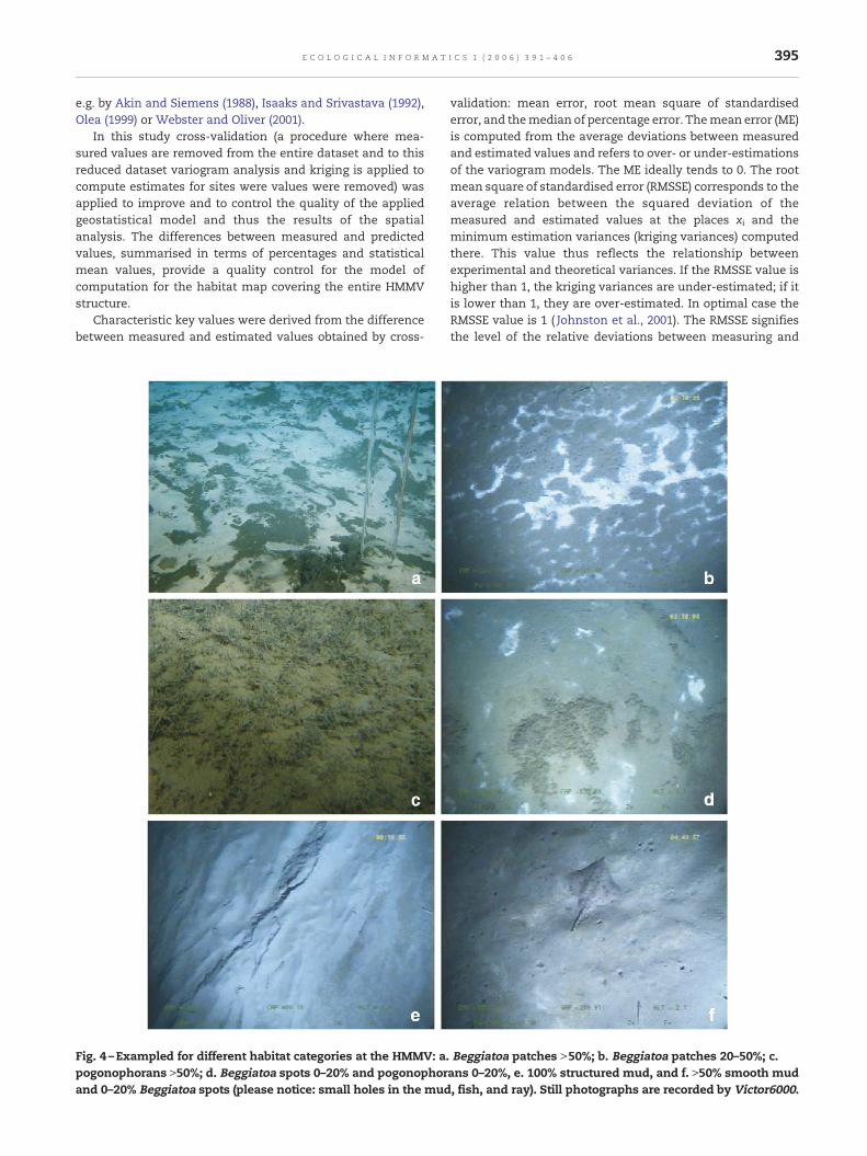
Fig. 4 –Exampled for different habitat categories at the HMMV: a.pogonophorans N50%; d. Beggiatoa spots 0–20% and pogonophorand 0–20% Beggiatoa spots (please notice: small holes in the mud

validation: mean error, root mean square of standardisederror, and themedian of percentage error. Themean error (ME)is computed from the average deviations between measuredand estimated values and refers to over- or under-estimationsof the variogram models. The ME ideally tends to 0. The rootmean square of standardised error (RMSSE) corresponds to theaverage relation between the squared deviation of themeasured and estimated values at the places xi and theminimum estimation variances (kriging variances) computedthere. This value thus reflects the relationship betweenexperimental and theoretical variances. If the RMSSE value ishigher than 1, the kriging variances are under-estimated; if itis lower than 1, they are over-estimated. In optimal case theRMSSE value is 1 ( Johnston et al., 2001). The RMSSE signifiesthe level of the relative deviations between measuring and

Beggiatoa patches N50%; b. Beggiatoa patches 20–50%; c.ans 0–20%, e. 100% structured mud, and f. N50% smooth mud, fish, and ray). Still photographs are recorded by Victor6000.

Table 1 – Categories applied formapping of biogeochemicalhabitats of the HMMV

Beggiatoa 0–20% Pogonophorans 0–20%

Mud smooth N50%

Beggiatoa 20–50% Pogonophorans 20–50%

Mud structuredN50%

Beggiatoa spots 20–50% PogonophoransN50%

Mud smooth 100%

Beggiatoa patches 20–50%

Mud structured100%

Beggiatoa spots N50%Beggiatoa patchesN50%

396 E C O L O G I C A L I N F O R M A T I C S 1 ( 2 0 0 6 ) 3 9 1 – 4 0 6

estimated values. If the respective measured value is definedas 100%, the difference between measured and estimatedvalue can be indicated in percent by the median of percentageerror (MPE). A low MPE generally indicates a low deviationbetween measured and predicted values and therefore areliable estimation model.

Based on the results of the data exploration and thevariogramanalyses, themeasured data are converted to surfacemaps. The suitable kriging method depends on the data type,the data distribution, the data properties, and the scientificquestion. Universal kriging for example is to be applied ifcomprehensible deterministic trends can be detected.

Indicator kriging (IK) is derived from ordinary kriging andusually used to divide values at locations to two categories bymeans of a threshold (cutoff) value (or multiple cutoff values):smaller than and larger than the threshold (converting the datafromametric scale intoanordinal scale).But IK isalsoperformedfor the spatial generalisation of geological or biological informa-tion,when categorical data as the occurrence/absence of benthicepifauna (e.g. Rivoirard et al., 2000) is studied.

In this study several coverage degrees of occurrences orabsence of chemoautotrophic communities (categories) areextracted from video material as polygons, which are used atthe outset. Each of the polygons is at a time selected for binaryinspection relating to the categories. In case of the occurrence ofthe certainspeciesor sediment type thevalue 1, and incaseof itsabsence the value 0 is assigned to the measuring location.Categorical data are thus converted into binary data before theinterpolation of the centroids of the polygons. With IK spatialprobability maps (one for each category) are computed for theoccurrence of the respective species or sediment type. Theinterpolation results can also be interpreted as the percentageprobabilities; for example: “with a probability of 85% muddysediment will occur”.

The combination of the categorymapswithin the GIS allowsthecomprehensiveviewongraduatedoccurrenceof e.g. bacterianot only onto one category provided typically by IK maps.

Fig. 5 –GIS-based overlay technique producing multi-parametric surfaces.

4. Material and methodical realisation

4.1. Data acquisition: georeferenced video mosaicing

During theRVPolarstern expeditionArcXIX3b (Klages et al., 2004) avideo system was attached at the bottom of the ROV Victor6000

(Ifremer) (Fig. 1). During the dives the position of the ROV wasdetermined by highly accurate Ultra Short Base Line (USBL)navigation system (Jouffroy andOpderbecke, 2004). The ROVwasoperated at amaximumaltitude of 3mabove seafloor (in awaterdepth of 1255 m to 1265 m) with a speed of 0.3 m s−1. The videosystemhad an optical aperture of 60°. At an altitude of 3maboveseafloor the video observations by the ROV has a width of 3 m,therefore. This ensured a high image quality and allowed real-time video mosaicing of the seafloor by the software MATISSE(Mosaicing Advanced Technologies Integrated in a Single Soft-wareEnvironment),whichwasdevelopedby theFrenchResearchInstitute for Exploitation of the Sea (Ifremer). During themosaicingprocess, onemosaic arises eachhalf aminutemergingabout 500 images recorded by the video camera. Each mosaiccovers an area of about 3 m of width and 6–7 m of length (pixelwidth 8.3 mm).

In total about 24 km of videomosaicingwere recorded duringsix ROV dives (35 hours dive time). MATISSE (Allais et al., 2004;Vincent et al., 2003) produces online digital merging georefer-enced mosaics (geotiffs) using the video input and the highprecision underwater navigation. A small displacement betweentwo consecutive images is required by the video mosaicingalgorithms based either on feature tracking (Shi and Tomasi,1994) or robust optic flowmethods (OdobezandBouthémy, 1994).The georeferencedmosaics are visualised and analysedwithin aGeographical Information System (GIS).

A total amount of 2840 mosaics was visually inspected; thedifferent biogeochemical habitats were identified and mappedas polygons on the video mosaics with the GIS. Variogramanalysis and kriging was applied to a so-called working datasetconsisting of 2310 images. The remaining 530 mosaics wereused for validation purpose which allows comparing theestimates derived by the geostatistical analysis with anadditional independent dataset.

4.2. Data analysis

The work flow for the development of three mono-parametricmaps (MPM) from image datawhich form the basis for a detailedhabitat map of the HMMV is represented in Fig. 3. As a first stepthe raster data consisting of 2840 georeferenced video mosaicsare imported into the GIS and areas of Beggiatoa, pogonophoransand uncovered mud are digitised as polygons (regionalisation).

Fig. 6 –GIS-based data simplification and data management.

397E C O L O G I C A L I N F O R M A T I C S 1 ( 2 0 0 6 ) 3 9 1 – 4 0 6

To each polygon the attribute (category) according to theclassification scheme (see below) was assigned. For a transfor-mation of polygons to point data the centroids coordinates of thepolygons and the assigned attributes are used for the interpo-lation by means of indicator kriging. By these means one rastermap was generated for each classification category (cell size3×3m). Finally, amono-parametricmap is createdwith the helpof GIS techniques, by a combination of all category maps of oneparameter (e.g. Beggiatoa). A further overlay of the mono-parametric maps (Beggiatoa, pogonophorans and uncoveredmud) can result in a detailed predictivemulti-parametric habitatmap for theHMMV. TheMPMs are used for an overlay to amulti-parametric habitat map, and area computations are conductedwith respect to the source location of mud flows and pattern ofbiogeochemical habitats allowing conclusions on the biogeo-chemistry of the HMMV (Jerosch et al., in press).

4.3. Habitat indicator coding and GIS implementation

By the video surveys a significant part of HMMV was coveredwhich allowed to identify and map sedimentological and biolog-ical features at the seafloor and the distribution of different bio-geochemical habitats as Beggiatoa, pogonophorans or mud flows.

Basically, the HMMV can be grouped into three majorspatial entities according to the habitat indicators: (i) uncov-eredmud of either a very youngmud flow, not yet inhabited byBeggiatoa, or old mud flow; (ii) occurrences of Beggiatoa whichindicates intense methane consumption (anaerobe oxidationof methane – AOM) taking place beneath the seafloor; (iii)pogonophorans indicating a lower CH4 consumption and oldermud flow. For the uncovered mud highest methane releaseinto the bottomwater is expected due to themissing “biofilter”by indicating Beggiatoa or pogonophoran population.

These three parameters determine the biogeochemicalhabitats at the HMMV. In addition Beggiatoa and pogonophor-ans occur together and form transition zones covered by e.g.Beggiatoa (coverage of 0–20%) and pogonophorans (coverageof N50%). The attribution for example assigning only thecategory pogonophorans 20–50% to an area, signifies automat-ically a 50 –80% uncovered mud fraction. Non-colonised mud,Beggiatoa, and pogonophorans (examples are shown in Fig. 4)were classified based on their degree of coverage (Table 1).

About 24 km (17 km working dataset and 7 km validationdataset) on 2840 georeferenced video mosaics were analysedby visual inspection loaded at a time into a GIS (ArcGIS 9.1,ESRI). The digitisation of the mosaic contents produces anenormous data reduction from raster data to vector datawhich is required for a further analysis.

The resulting 1578 polygons were featured with thecontents of the mosaics concerning the classification schemein Table 1. All categories given there are coded binary relatedto their occurrence in the dataset and surface maps arecalculated using the centroids of the polygons by means of IKfor all 13 categories. The combination of the category maps ofone parameter (e.g. Beggiatoa) yields into a mono-parametricmap. The MPMs in general are the basis for multi-parametricoverlay maps. Two or more spatially overlapping input datalayers of geometrical type polygon, line or point will beoverlaid geometrically producing a new multi-parametricdata layer (Fig. 5). A GIS-based overlay of all MPMs wouldreveal e.g. in a transition zone of Beggiatoa and pogonophoransand thus in a complex view of the habitat distribution of theHMMV.

The analysis of the imageswas done bymeasuring the extentof specific items as spots (b30 cm) and patches (N30 cm) ofbacteria, pogonophorans or mud within the GIS. Areas are

Fig. 7 –Data distribution of the parameters Beggiatoa, pogonophorans and uncovered mud corresponding to polygons of theworking datasets (Fig. 8d). The number of polygons (n), the area (A) which is covered by the parameter, the averaged area of onepolygon (MA), and the ratio areas of coverage to the total area of investigation (A/TA) with regard to the parameter. Areas aregiven in m2.

398 E C O L O G I C A L I N F O R M A T I C S 1 ( 2 0 0 6 ) 3 9 1 – 4 0 6

digitisedaspolygons (Fig. 6)with respect to thedefinedcategories,and are provided with keywords concerning their habitatindicating characteristics andmetadata. For the indicator krigingprocedure each category is to be coded binary regarding to itsoccurrence (yes=1 or no=0). All the information was storedwithin a relational geodatabase system (Fig. 6).

5. Results

The results of this study are presented in two steps: first thepresentation of the resulting working dataset, the generatedMPMs including variogram analysis and the visual control of

Fig. 8 – (a–d) Distribution of analysed polygons and predictive surfaces after indicator kriging: (a) Beggiatoa, (b) pogonophorans, and (c) uncovered mud. Colours are arrangedgradually concerning their probability of occurrence (Table 2). Polygons appear as lines with respect to the scale of the map. If no significant differences can be recognisedbetween the appearing lines and the interpolated surfaces, the variogrammodel fits well. Blank areas indicate a probability of occurrence less than the lowest probability valuegiven in the legend. (d) Data distribution of the entire working dataset. The encircled area provides an example for a reliable fit, whereas within the rectangles thecorrespondence between observed and predicted categories is weaker (for details see text).

399EC

OLO

GIC

AL

IN

FO

RM

AT

IC

S1

(2006)

391–406

Table 2 – Absolute and relative values of the interpolated surfaces at the HMMV

HI coverage degree Interpolatedareas [m2]

Percentof

coverage

Probability of occurrence in %

User defined GIS calculated

Min Max Mean

Pogon. Pogonophorans no 297,746 24.49 70 100 92Pogonophorans 0–20% 36,649 3.01 70 100 90Pogonophorans 20–50% 43,295 3.56 70 100 84Pogonophorans N50% 276,121 22.71 70 100 93

Beggiatoa Beggiatoa not predicted 304,424 26.68Beggiatoa no 318,745 27.93 70 100 87Beggiatoa 0–20% 250,200 21.92 70 100 80Beggiatoa 20–50% 163,077 14.29 70 100 83Beggiatoa spots 20–50% 43,815 3.84 70 96 76Beggiatoa patches 20–50% 22,699 1.99 70 100 76Beggiatoa N50% 29,078 2.55 40 86 69Beggiatoa spots N50% 2357 0.21 40 50 41Beggiatoa patches N50% 6809 0.60 40 100 44

Mud Mud all N50% 689,563 58.39 70 100 96Mud smooth N50% 276,917 17.02 70 100 85Mud structured N50% 12,256 23.45 70 100 92Mud smooth 100% 200,974 0.10 40 45 41Mud structured 100% 1182 1.04 70 99 76

The mean probability of occurrence of each parameter category is calculated by the GIS. The minimum and maximum thresholds are userdefined and correspond to the areas shown in the Fig. 8a–c. The deviating total areas are caused by the individual category variograms used forthe interpolation.

Table 3 – Quality of estimation by means of statisticalaverage values resulting from cross-validation

Parameter ME⁎10−3 RMSSE MPE

Beggiatoa no −1.588 1.009 16.12Beggiatoa 0–20% −0.354 1.004 36.52Beggiatoa 20–50% 0.184 0.998 8.02Beggiatoa spots N50% 0.080 1.090 2.11Beggiatoa patches N50% −0.014 1.047 0.00Pogonophorans no 0.145 0.990 4.85Pogonophorans 0–20% −2.880 1.001 9.56Pogonophorans 20–50% −5.836 0.997 30.34Pogonophorans N50% 0.618 1.008 30.17Mud all N50% −1.681 1.038 31.16Mud smooth N50% −2.044 1.002 35.85Mud structured N50% −0.572 0.986 0.00Mud smooth 100% 0.029 0.989 0.00Mud structured 100% 0.074 0.973 0.00

400 E C O L O G I C A L I N F O R M A T I C S 1 ( 2 0 0 6 ) 3 9 1 – 4 0 6

the interpolated surfaces using the working datasets. Thesecond step consists of a validation of the quality of the MPMswhich is performed by cross-validation of the indicator krigingmodels and visual inspection using a validation dataset offurther analysed video mosaics.

5.1. Predictive mono-parametric habitat maps at theHMMV

The working dataset is made up by 2310 of the 2840 visuallyinspected video mosaics. They are analysed with regard to thecoveragedegree of theparametersBeggiatoa, pogonophoransanduncovered mud. The resulting dataset consisting of 1578polygons is used for the compilation of the three mono-parametric maps within GIS. The working dataset correspondsto a total area of investigation (TA) of 45,790 m2 (15.3 km ROVtransect×3m imagewidth). Thedistributionof thedata assignedto the respective parameter categories is given in Fig. 7. Forexample, the category Beggiatoa spots 0–20% is representedmostfrequently (number of polygons (n) is 595) covering an area of6751m2 (A). Theaveragearea (MA)of onepolygonof this categorycovers an average area of 28 m2 (Beggiatoa spots, defined asb30 cm, are clustered into areas). Furthermore, this category isassigned to 36% (A/TA=0.36) of the total area of investigation.Including the categories “no Beggiatoa” (33%) and Beggiatoapatches 0–20% (15%) these three categories represent themajority (84%) of the analysed surface. The spatial distributionof the working dataset is shown in Fig. 8. The polygons,representing the video mosaicing tracks as shown in Fig. 6,there appear as lines with respect to the scale of the map.

According to Journel and Huijbregts (1978) the variogramcalculations were performed exclusively for distances belowhalf of the maximum horizontal extension of the area underinvestigation (here ∼0.7 km). Cross-validation was used as the

method toselect theoptimumvariogrammodel: itwas intendedto minimise MPE and concomitantly approximate ME toward 0and RMSSE toward 1. For the surface calculations the meandistance of each observation site to its nearest neighbour wasused as the cell (lag) size. The number of lags allocated to eachlag size was adjusted to ensure that significant autocorrelation(range) became clearly visible in the variogram window. If thesemivariances displayed on the variogram map indicatedanisotropies in the data field, different ranges for differentdirections (to account for anisotropies) were compared witheach other.

For the kriging calculations the raster was set according totheaveragemeandistance of eachmeasurement site in relationto its nearest neighbour. The searching or variogram windowwithin measured values were included to estimate a certain

Fig. 9 – (a–c) Results computed by cross-validation: visualisation of percentage errors and median percentage errors (MPE). Theabscissa gives number of polygons and the ordinate the conformance betweenmeasured and predicted values after a full cross-validation of 1578 polygons (note the scale of the ordinate is inverted).

401E C O L O G I C A L I N F O R M A T I C S 1 ( 2 0 0 6 ) 3 9 1 – 4 0 6

point was adjusted to the range of the variogrammodel. A four-sector neighbourhood was defined to avoid directional bias.

After the IK interpolation the combination of the categorymaps results in three MPMs (Fig. 3). The MPMs contain the pre-dictive surfaces at the HMMV that are covered by the parameter,respectively (Fig. 8a–c). Each MPM is colour coded distinctivelyaccording to the different categories (e.g. yellow: Beggiatoa 0–20%coverage, orange: Beggiatoa 20–50% coverage and red: Beggiatoa50% coverage). The degrees of occurrence probability is thengradually arranged (light yellow corresponds to a smallerprobability than dark yellow, etc.). Blank areas do not imply nooccurrence of the parameter, but a probability occurrence less

than e.g. 70%, respectively to the minimum thresholds given inTable 2. No occurrence areas are indicated apart.

Visual controlof the interpolatedsurfacescanbeperformedbyoverlaying the polygons of the working dataset with the rastermaps. For this purpose, theworkingdataset is coloured equally tothe parameter categories (Fig. 8a–c). If no significant differencescan be recognised between the appearing lines and the interpo-lated surfaces, the variogram model is well fitted to the data(encircledarea inFig. 8a).Atothersites–apparentlyatallMPMs–avisual impressionofunderestimatearises,and it seemsthatblankregions should have been assigned to a parameter category. Thisimpression results from the ambitious defined minimum

Fig. 10 – (a–d) Validation dataset combined with simplified mono-parametric maps. (a) Beggiatoa, (b) pogonophorans and (c) uncovered mud. (d) distribution of the entirevalidation dataset. Significant deviations of the validation polygons to the MPMs are highlighted by rectangles.

402EC

OLO

GIC

AL

IN

FO

RM

AT

IC

S1

(2006)

391–406

403E C O L O G I C A L I N F O R M A T I C S 1 ( 2 0 0 6 ) 3 9 1 – 4 0 6

threshold of occurrence probability (Table 2). Blank area are thusnot assigned to no category but to a probability of occurrence lessthan a 70%, for example, for themud classes (note legends in Fig.8).

The IK interpolation produces probability values for theoccurrence of a feature between 0 and 1. They weretransformed into percentages (Table 2). Both surfaces withhigh probability of occurrence as well as surfaces with highprobability of exclusion of the parameter category can beassigned. Minimum and maximum threshold values aredefined manually oriented on the calculated mean probabil-ity values. The average value gives the overviewof the generalestimation quality; the minimum and maximum thresholdvalues are important because they correspond directly withthe areas and their graduated colours in the MPM (Fig. 8a–c).Table 2 contains the three values associated to eachparameter category and gives, therefore, information aboutthe interpolated surfaces.

In general reasonable results in nearly all analysed para-meter categories were achieved, except in the categories of,“Beggiatoa N50%” and “smooth mud 100%”. Here the resultscontain a certain degree of uncertainty.

5.2. Validation of the results applying cross-validationand a validation dataset

When performing validation, two datasets are used: a workingand a validation dataset. The working dataset contains themeasured locations on which the variogram analysis appliedfor prediction is based. Calculated statistics, resulting fromleave-one-out cross-validation, serve as diagnostics thatindicate whether the model and its associated parametervalue are reasonable.

The validation dataset is used to prove the interpolatedpredictions independently from the variogram analysis by theresults of the visual inspection of further 530 video mosaics.

5.2.1. Evaluation of the prediction models (variograms)derived from cross-validationThe so-called leave-one-out cross-validation involves sub-tracting a single observation from the working dataset andcalculating this single observation from the remaining obser-vations. This is repeated such that each observation in theworking dataset is used once as the single observation. Such across-validation was applied for each of the 13 binary codedcategories (Table 1) predicting each of the polygons of theworking dataset by using the specific variograms. This allowscomparison of results derived by the reduced dataset with theresults derived by the complete working dataset. From thecross-validation errors the percentage conformance (and/ordeviation) were expressed as single values for each parametercategory; their median value is defined as the medianpercentage error (MPE). Furthermore, three averaged keyparameters are calculated from the distribution to character-ise the quality of the chosen variogram models (Table 3).

The graphs in Fig. 9a–c show the percentage error of thesingle values for selected categories grouped by parameter.These single values result from a full cross-validation,predicting each of the 1578 polygons (X-axis) by the help ofthe reduced dataset and the percentage differences between

measured and predicted values. The percentage of confor-mance is given then on the y-axis. For instance, 1361 of the1578 polygons of the category Beggiatoa spots N50% (blue line)are forecast accurately (100%). The graph intersects theordinate at an x-value of 1545 polygons, signifying a confor-mance of these polygons of 80% with the variogram model.

Considering graphs in Fig. 9a–c the variograms fit partic-ularly well with the categories Beggiatoa N50% and mud 100%coverage. In these categories the majority of the polygons(more than 1000 of 1578) coincide to 100% comparingexamined and predicted values: 1361 polygons of the categoryBeggiatoa spots N50% are predicted precisely, as well as 1033polygons of Beggiatoa patches N50%, 1030 polygons of mud all100%, 1085 polygons of smooth mud 100%, and 1435 polygons ofstructured mud 100%. For the category Beggiatoa spots N50%further 71 polygons are predictedwith up to 90% conformance,i.e. 1432 of 1578 polygons (90.8%) are well determined (Fig. 9a).Furthermore, the quality of the tube worm estimation modelappears visibly in a reliable way for the categories “nooccurrence of pogonophorans” and “pogonophoran coverage0–20%”, while the other two categories (20–50% and 50%) arerepresented rather moderately (Fig. 9b).

The performed averaged key values are summarised inTable 3, which demonstrates among others the ME, RMSSEand the MPE values. Both the ME and the RMSSE indicateneither crucial under- nor over-estimation and, therefore, nobias in the surface estimations: ME shows that the averagecross-validation errors equal almost zero and RMSSE equalsalmost 1 in all cases. TheMPE can be observed to be low for thecategories: mud structured N50%; mud smooth 100%; mudstructured 100%; Beggiatoa 20–50%; Beggiatoa spots N50%, andBeggiatoa patches N50%. Highest MPE are found for Beggiatoa0–20% and mud smooth N50%.

5.2.2. Estimation of the predictive mono-parametric mapsusing a validation datasetSubsequent to the statistic estimate of the quality of therespective IK model, the final control of the resulting IKsurfaces follows with help of a validating dataset. This datasetwas not used for the determination of the geostatistical datastructure and thus gives pure information whether theinterpolated surfaces approximate to further analysed data.

The validating dataset consists of an examined surface of9358m2, which is transformed into 675 polygons, resulting fromthe visual analysis of 530 videomosaics. Therefore, a fifth of the2840 examined mosaics were used as controlling dataset. InFig. 10a–c the results of this investigation are intersected withthe kriged surfaces of the MPM enabling a direct comparison.Fig. 10d shows the spatial distribution of the working dataset inblack and the validation dataset in white colours.

Deviations become visible for all three parameters, but theagreements outweigh and confirm the general spatial struc-ture of the data, and/or the spatial distribution of theprobability of occurrence. In case of Beggiatoa it is noticeablethat particularly in the north and north-east of the HMMVcentre (see rectangles in Fig. 10a) the interpolated surfacesrepresent rather an over-estimation of the bacteria occur-rence. In these areas it becomes clear – on the basis of thevalidating data record – that pogonophorans are certainlyoutbalanced there (rectangles Fig. 10b). However, the

404 E C O L O G I C A L I N F O R M A T I C S 1 ( 2 0 0 6 ) 3 9 1 – 4 0 6

exclusion surfaces of these two parameters are predictedparticularly well. The validation polygons of the parametermud (Fig. 10c) particularly underline occurrences of uncoveredsurfaces in the centre of the HMMV. Here, the polygons clarifythat an underestimation of this parameter is probably thecase. Note that at the blank areas the mud categories are notexcluded, but attributed to a probability of occurrence of lessthan 70%.

6. Discussion

The representation and area calculation of irregularly distrib-uted data is in the focus of all territorial geochemicalbalancing methods or definition of protection zones. Thesurface exactness of specific oceanic regions, as the estimateof global marine primary production (Longhurst, 1998),benthic material flux (Zabel et al., 2000), or the distributionof chemoautotrophic organism is always related to surfaceareas. Therefore, the interpolation of points into surfacesrepresents an important gain of information. Resulting mono-parametric maps are the basis for complex multi-parametricmaps. For this purpose the quality assessment of the MPMs isan important factor.Within this study statistical (IK and cross-validation) and visual (working and validation polygons)methods were used to generate surface maps describing thespatial distribution of three parameters occurring at theHMMV. These methods enable to evaluate the quality of themono-parametric maps with regard to the Tables 2 and 3 aswell as in the Figs. 8–10.

The average probability values in Table 2, calculated withinthe GIS, describe very credible values for all Beggiatoacategories except for “spots and patches N50%”. Fig. 8 corre-lates directly with Table 2, i.e. all represented Beggiatoasurfaces (Fig. 8a) except “spots and patches N50%” arepredicted with high values and thus with high probability ofoccurrence. “Spots and patches 50%” surfaces represented inFig. 8a are predicted with less probability than the remainingBeggiatoa categories. Even these surfaces are provided withreliable MPE values indicating high conformance betweenmeasured and predicted values (Table 3 and Fig. 9a) and a highquality of the applied IK models. This combination suggeststhat the prediction of these surfaces is limited regionally;assigning a colonisation density closely related to certaingeochemical conditions. This assumption is confirmed by theregional distribution of the Beggiatoa categories N50% alsowithin the validation dataset illustrated in Fig. 10a.

On the basis of the graphs in Fig. 9a the quality of theestimation model appears for each category. It can bedetermined which of the IK models worked in a confidentialway by the percentage errors derived from cross-validation.Such a representation of the single percentage errors helps tomake the interpolated maps more transparent. All Beggiatoacategories achieve satisfying MPE values, only the MPE for thecategory 20–50% coverage turned out comparatively high(Table 3). This class is the most frequently occurring classwithin the working dataset (Fig. 7), which is spatially distrib-uted on a large area. This could explain the high probabilityaverage valueof occurrence (Table 2) for the areas in Fig. 8a, butalso the fuzziness of the IK of model for that category.

The distribution of the forecast surfaces which are notcovered by the bacteria is limited to the region outside of theHMMV. This could be confirmed neither by visual videomosaic analysis (concerned surface are highlighted by arectangle in Fig. 8a) nor during the ROV dive experiences ofscientists. It is known that in the centre of the HMMV a surfaceexists completely uncovered by Beggiatoa or pogonophorans.On the result map Beggiatoa are not excluded which would bethen assigned by shaded surfaces (rectangle Fig. 8a). Never-theless, areas are blank resulting from the adjusted minimumthreshold in Table 2. Regarding to this region concerning thetwo other parameters, pogonophorans are also excluded there(rectangle Fig. 8b), but for mud a probability of over 70% iscalculated (rectangle Fig. 8c). Concluding reversely, theprobability of occurrence for Beggiatoa is only 30% maximum.

The category Beggiatoa 20–50% attains both a good estimatefor the interpolated probability of occurrence values and forthe cross-validation average values. Furthermore, this cate-gory achieves applicable results also after the control usingthe validation polygons.

For all pogonophoran surfaces in Fig. 8b reliable probabilityof occurrence average values could be determined with thehelp of cross-validation procedures (Table 2). However, the IKmodel is of a better quality in the categories no pogonophor-ans and 0–20% coverage than for the other two classes (20–50%and N50%). Thus, the surfaces of the two latter categories arepredicted more uncertainly than those of the first mentioned.Regarding the pogonophoran distribution within the workingdataset, a conspicuous region is observed in the northwest ofthe HMMV where a too small spreading of the interpolatedsurface is probable. This impression is affirmed by thevalidating dataset (rectangles Figs. 8b and 10b).

The validating dataset shows that the data distribution ofthe working dataset used for IK led to further insufficientestimates in the interpolated surfaces northeast of the mudvolcano centre (rectangles Figs. 8b and 10b). There, it becomesapparent that the pogonophoran surfaces N50% shouldprobably have been predicted more extensively to the centreof the mud volcano, while the Beggiatoa 20–50% surfaces wereprobably computed too expanded.

Evaluating all applied control mechanisms (visually pre-dicted on the basis the Figs. 8b and 10b and statistically on thebasis the Tables 2 and 3), the kriged surfaces which are notcolonised by pogonophorans are predicted reliably: bothoutside of the HMMV (reasonable by missing geochemicalcharacteristics of the sediment pore water) and in the centralmud volcano area (justified by high temperatures, fresh mudflows and a temporal hierarchy in the colonisation structure ofthe chemoautotrophic organisms Beggiatoa and pogonophor-ans) (Jerosch et al., in press).

A special ecological meaning is attached to the uncoveredand almost uncovered surfaces in the active centre of themudvolcano, because the highest methane release into thehydrosphere is expected due to the absence of biofilterindicating chemoautotrophic communities (Boetius et al.,2000; Damm and Budéus, 2003; De Beer et al., in press). Thedata distribution of the completely uncovered mud surfaces(mud 100%), in addition, the category mud all 50% is wellconverted into the IK models (Table 2), while the lowprobability of occurrence does not permit a supra-regional

405E C O L O G I C A L I N F O R M A T I C S 1 ( 2 0 0 6 ) 3 9 1 – 4 0 6

interpretation of surfaces in the MPM (similar to the Beggiatoacategories N50%). Also the graphs of the percentage errors ofthese five classes are quite similar (Fig. 9a and c). The mudcategories show that the MPE is not always meaningfulenough, as to be seen by the example of the comparison ofthe categories “50% structured, 100% smooth, and 100%structured”. All three MPEs are 0 (Table 2); only the individualpercentage error values classify a qualitative order, which isalso reflected in the ME values. Hence, the IK model of thecategory smooth mud 100% is adapted best to the datadistribution.

The data density (high and sporadically arising) hasdifferent weight of impact due to the IK function in the area(e.g. Richmond, 2005; Webster and Oliver, 2001). According tovisual impressions of the validating evaluation, the mudsurfaces seem to be slightly underestimated in the centre ofthe HMMV (see rectangle in Fig. 10c). Conducting an interpo-lation with both datasets would probably be more expandedand the individual central mud surfaces would be thenconnected to one large area as, for instance the polygondrawn manually in Fig. 10c.

7. Conclusions

Based on a rather dense dataset information about non-sampled seafloor areas is predicted with the help of thegeostatistical method indicator kriging. This could be con-ducted successfully due to a large amount of exclusive videomosaics taken up with the ROV Victor6000, which wereprovided furthermore with geographical coordinates. Dataacquisition with a ROV is a time- and cost-intensive work. Theapproach was to extract categorical information from imagedata, to transform them into binary coded (0/1) discretevariables and to extrapolate them GIS-based into mono-parametric surface maps.

Interpolationprocedure represents again in informationoverunsampled areas, however, with the restriction that the resultsalways remain a degree of uncertainty; therefore interpolationcannot replace real measured values and the result of aninterpolation becomes ever better, the more largely the useddata density. However, this uncertainty can be made moretransparent by the presented approach identifying the weakpoints but also the strengths of interpolatedmaps (Atkinson andLloyd, 1998; Rufino et al., 2005). Recapitulatory, the quantity ofthe analysed data allows the partitioning into a working and avalidating dataset and bears a cross-validation. We achievedreliable results andevaluatedonly smalldeviations inour resultsusing sophisticated high minimum probability values.

Even the refined analysis procedure (transforming rasterdata into regionalisation polygons and points, use of geostatis-tics, and the GIS overlay technique) contains acceptabledeviations the results supply the first surface maps of theHMMV. They are used in Jerosch et al. (in press) in form of apredictive multi-parametric map after a GIS-based overlay ofBeggiatoa, pogonophorans and uncovered mud. This map isused for area computations with respect to the source locationof mud flows and pattern of biogeochemical habitats. Discuss-ing the quality of surface maps is thus also tool to evaluatefollowing continuative studies.

The maps developed in this study are considered as aguideline for further expeditions to the HMMV. For earlierhabitat studies at the HMMV please refer to e.g. Gebruk et al.(2003) and Milkov et al. (1999, 2004).

Submarinemud volcanoes occur worldwide. Together withsubmarine asphalt volcanism sites (MacDonald et al., 2004)they provide the geochemical conditions (e.g. gas hydrates,methane release) creating habitats for chemosynthetic life(bacteria and tube worms). For example the Milano MudVolcano of the Central Mediterranean Ridge (Huguen et al.,2005) and the Chapopote Asphalt Volcano in the CampecheKnolls, Gulf of Mexico, (Hovland et al., 2005; MacDonald et al.,2004) are potential study areas for similar evaluation proce-dures as conducted at the HMMV.

Acknowledgements

The authors thank all crew members and scientists onboardRV Polarstern and the Genavir team of ROV Victor6000 fortheir unremitting assistance. We are grateful to the Ifremercolleagues A.G. Allais, P. Siméoni, L. Méar for the technicalsupport during the video mosaicing surveys. This study wasperformed in the framework of the R&D-Programme GEO-TECHNOLOGIEN funded by the German Ministry of Educationand Research (BMBF) and German Research Foundation (DFG)as well as the AWI-Ifremer bilateral collaboration programme.This is publication no. GEOTECH-204.

R E F E R E N C E S

Akin, H., Siemens, H., 1988. Praktische Geostatistik. Springer-Verlag, Berlin-Heidelberg. 304 pp.

Allais, A.-G., Borgetto, M., Opderbecke, J., Pessel, N., Rigaud, V., 2004.SeabedvideomosaicingwithMATISSE: a technical overviewandcruise results. Proceedings of 14th International Offshore andPolar Engineering Conference, ISOPE-2004, Toulon, France, May23–28 2004, vol. 2, pp. 417– 421.

Atkinson, P.M., Lloyd, C.D., 1998. Mapping precipitation inSwitzerland with ordinary and indicator kriging. Journalof Geographic Information and Decision Analysis 2 (2),65–76.

Boetius, A., Ravenschlag, K., Schubert, C.J., Rickert, D., Widdel, F.,Gieseke, A., Amann, R., Jørgensen, B.B., Witte, U.,Pfannkuche, O., 2000. A marine microbial consortiumapparently mediating anaerobic oxidation of methane.Nature 407, 623 – 626.

Boetius, A., Beier, V., Niemann, H., Müller, I., Heinrich, F., Feseker, T.,2004. Geomicrobiology of sediments and bottom waters of theHåkonMosbyMudVolcano. In:Klages,M., Thiede, J., Foucher, J.-P.(Eds.), The Expedition ARK XIX/3 of the Research Vessel“Polarstern” in 2003. Reports on Polar and Marine Research,vol. 488, pp. 190–199.

Damm, E., Budéus, G., 2003. Fate of vent-derived methane inseawater above the Håkon Mosby Mud Volcano (NorwegianSea). Marine Chemistry 82, 1–11.

Davis, J.C., 2002. Statistics and Data Analysis in Geology, 3rd ed.John Wiley and Sons, New York. 638 pp.

DeBeer,D., Sauter, E.,Niemann,H.,Witte,U., Schlüter,M., Boetius,A.,in press. In situ fluxes and zonation of microbial activity insurface sediments of the Håkon Mosby Mud Volcano. Limnologyand Oceanography.

406 E C O L O G I C A L I N F O R M A T I C S 1 ( 2 0 0 6 ) 3 9 1 – 4 0 6

Dimitrov, L.I., 2002. Mud volcanoes—themost important pathwayfor degassing deeply buried sediments. Earth-Science Reviews59, 49–76.

Eldholm,O., Sundvor, E., Vogt, P.R., Hjelstuen, B.O., Crane, K., Nilsen,A.K., Gladczenko, T.P., 1999. SW Barents Sea continental marginheat flowandHåkonMosbyMudVolcano.Geo-Marine Letters 19,29–37.

Fleischer, P., Orsi, T.H., Richardson, M.D., Anderson, A.L., 2001.Distribution of free gas inmarine sediments: a global overview.Geo-Marine Letters 21, 103–122.

Gebruk,A.V., Krylova, E.M., Lein,A.Y.,Vinogradov,G.M.,Anderson, E.,Pimenov, N.V., Cherkashev, G.A., Crane, K., 2003. Methaneseep community of the Håkon Mosby Mud Volcano (theNorwegian Sea): composition and trophic aspects. Sarsia 88,394–403.

Hjelstuen, B.O., Eldholm, O., Faleide, J.I., Vogt, P.R., 1999. Regionalsetting of Håkon Mosby Mud Volcano, SW Barents Sea margin.Geo-Marine Letters 19, 22–28.

Hovland, M., MacDonald, I.R., Rueslâtten, Johnsen, H.K., Naehr, T.,Bohrmann, G., 2005. Chapopote Asphalt Volcano may havebeen generated by supercritical water. EOS 86 (42), 397–399.

Huguen, C., Mascle, J., Woodside, J., Zitter, T., Foucher, J.P., 2005.Mud volcanoes and mud domes of the Central MediterraneanRidge: near-bottom and in situ observations. Deep-Sea Re-search. Part 1. Oceanographic Research Papers 52, 1011–1931.

Isaaks, E.H., Srivastava, R.M., 1992. An Introduction to AppliedGeostatistics. Oxford University Press. 561 pp.

Jerosch, K., Schlüter, M., Foucher, J., Allais, A., Klages, M., Edy, C.,in press. Spatial distribution of mud flows, chemoautotrophiccommunities, and biogeochemical habitats at Håkon MosbyMud Volcano. Marine Geology.

Johnston, K., Ver Hoef, J.M., Krivoruchko, K., Lucas, N., 2001. UsingArcGIS Geostatistical Analyst. ESRI, Redlands, USA. 40 pp.

Jouffroy, J., Opderbecke, J., 2004. Underwater vehicle trajectoryestimation using contracting PDE-based observers. AmericanControl Conference (ACC 2004), Boston.

Journel, A.G., Huijbregts, C.J., 1978. Mining Geostatistics. AcademicPress, London. 600 pp.

Klages, M., Thiede, J., Foucher, J.-P., 2004. The Expedition ARK XIX/3 of the Research Vessel “Polarstern” in 2003. Reports on Polarand Marine Research, vol. 488. 346 pp.

Kopf, A.J., 2002. Significance of mud volcanism. Reviews ofGeophysics 40 (2), 1005. doi:10.1029/2000RG000093.

Levin, L.A., Ziebis, W., Mendoza, G.F., Growney, V.A., Tryon, M.D.,Brown, K.M., Mahn, C., Gieskes, J.M., Rathburn, A.E., 2003.Spatial heterogeneity of macrofauna at northern Californiamethane seeps: influence of sulphide concentration and fluidflow. Marine Ecology. Progress Series 265, 123–139.

Longhurst, A., 1998. Longhurst Areas: Ecological Geography of theSea. Academic Press. 398 pp.

MacDonald, I.R., Bohrmann, G., Escobar, E., Abegg, F., Blanchon, P.,Blinova, V., Brückmann, W., Drews, M., Eisenhauer, A., Han, X.,Heeschen, K., Meier, F., Mortera, C., Naehr, T., Orcutt, B.,Bernard, B., Brooks, J., De Faragó, M., 2004. Asphalt volcarismand chemosysthetic life in the Campeche Knolls, Gulf ofMexico. Science 304, 999–1002.

Matheron, G., 1963. Principles of geostatistics. Economic Geology58, 1246–1266.

Milkov, A.V., 2000. Worldwide distribution of submarine mud vol-canoes and associated gas hydrates. Marine Geology 167, 29–42.

Milkov, A.V., Vogt, P.R., Cherkashev, G., 1999. Sea-floor terrains ofHåkonMosby Mud Volcano as surveyed by deep-tow video andstill photography. Geo-Marine Letters 19, 38–47.

Milkov, A.V., Vogt, P.R., Crane, K., Lein, A.Y., Sassen, R., Cherka-shev, G.A., 2004. Geological, geochemical, and microbialprocesses at the hydrate-bearing Håkon Mosby mud volcano: areview. Chemical Geology 205, 347–366.

Odobez, J.M., Bouthémy, P., 1994. Robust multi-resolution esti-mation of parametric motion models applied to complexscenes. IRISA Intern Report. 788 pp.

Olea, R.A., 1999. Geostatistics for Engineers and Earth Scientists.Kluwer Academic Publishers, Boston. 328 pp.

Pimenov, N., Savvichev, A., Rusanov, I., Lein, A., Egorov, A., Gebruk, A.,Moskalev, L., Vogt, P., 1999. Microbial processes of carbon cycle asthe base of food chain of Håkon Mosby Mud Volcano benthiccommunity. Geo-Marine Letters 19, 89–96.

Richmond, A., 2005. An alternative implementation of indicatorkriging. Computers and Geosciences 28, 555–565.

Rivoirard, J., Simmonds, E.J., Foote, K., Fernandes, P., Bez, N., 2000.Geostatistics for Estimating Fish Abundance. BlackwellScience, UK. 216 pp.

Rufino, M.M., Maynou, F., Abelló, P., Gil de Sola, L., Yule, A.B., 2005.The effect of methodological options on geostatistical model-ling of animal distribution: a case study with Liocarcinusdepurator (Crustacea: Brachyura) trawl survey data. FisheriesResearch 76, 252–265.

Sahling, H., Rickert, D., Lee, R.W., Linke, P., Suess, E., 2002.Macrofaunal community structure and sulfide flux at gashydrate deposits from the Cascadia convergent margin, NEPacific. Marine Ecology. Progress Series 231, 121–138.

Shi, J., Tomasi, C., 1994. Good features to track. Proceedings of theIEEE Conference on Computer Vision and Pattern Recognition(CVPR94), Seattle, WA, pp. 593–600.

Sibuet, M., Olu, K., 1998. Biogeography, biodiversity and fluiddependence of deep-sea cold-seep communities at active andpassive margins. Deep-Sea Research. Part 2. Topical Studies inOceanography 45, 517–567.

Smirnov, R.V., 2000. Two new species of pogonophoran from theArctic mud volcano off northwestern Norway. Sarsia 85,141–150.

Vincent, A.G., Jouffroy, J., Pessel, N., Opderbecke, J., Borgetto, M.,Rigaud, V., 2003. Real-time georeferenced videomosaicingwiththe MATISSE system. Proceedings of the Oceans 2003 MarineTechnology and Ocean Science Conference, MTS/IEEEOCEANS’03, San Diego, USA, September 22–26 2003, vol. 4,pp. 2319–2324.

Vogt, P.R., Gardner, J., Crane, K., 1999. The Norwegian–Barents–Svalbard (NBS) continental margin: introducing a naturallaboratory of mass wasting, hydrates and ascent of sedimentpore water and methane. Geo-Marine Letters 19, 2–21.

Webster, R., Oliver, M.A., 2001. Geostatistics for EnvironmentalScientists. John Wiley and Sons. Ltd, Chichester, New York.286 pp.

Zabel, M., Hensen, C., Schlüter, M., 2000. Back to the ocean cycles:benthic fluxes and their distribution patterns. In: Schulz, H.D.,Zabel, M. (Eds.), Marine Geochemistry. Springer–Verlag, Berlin–Heidelberg. 455 pp.