Spatial aggregation Data model and implementation · Spatial aggregation: Data model and...

ARTICLE IN PRESS

Contents lists available at ScienceDirect

Information Systems

Information Systems 34 (2009) 551–576

0306-43

doi:10.1

� Cor

Tel./fax:

E-m

sofie.ha

(B. Kuij

journal homepage: www.elsevier.com/locate/infosys

Spatial aggregation: Data model and implementation

Leticia Gomez c, Sophie Haesevoets a, Bart Kuijpers b, Alejandro A. Vaisman b,d,�

a Luciad NV, Belgiumb Hasselt University and Transnational University of Limburg, Belgiumc Instituto Tecnologico de Buenos Aires, Argentinad Universidad de Buenos Aires, Argentina

a r t i c l e i n f o

Article history:

Received 25 May 2008

Received in revised form

13 December 2008

Accepted 11 March 2009

Recommended by: L. Wongthe GIS. This approach allows both aggregation of geometric components and

Keywords:

Data warehousing

OLAP

GIS

Aggregation

79/$ - see front matter & 2008 Elsevier B.V. A

016/j.is.2009.03.002

responding author at: Universidad de Bueno

+54114902 0421.

ail addresses: [email protected] (L. Gomez),

[email protected] (S. Haesevoets), bart.ku

pers), [email protected] (A.A. Vaisman).

a b s t r a c t

Data aggregation in Geographic Information Systems (GIS) is a desirable feature, only

marginally present in commercial systems nowadays, mostly through ad hoc solutions.

We address this problem introducing a formal model that integrates, in a natural way,

geographic data and non-spatial information contained in a data warehouse external to

aggregation of measures associated to those components, defined in GIS fact tables.

We define the notion of geometric aggregation, a general framework for aggregate

queries in a GIS setting. Although general enough to express a wide range of (aggregate)

queries, some of these queries can be hard to compute in a real-world GIS environment

because they involve computing an integral over a certain area. Thus, we identify the

class of summable queries, which can be efficiently evaluated replacing this integral with

a sum of functions of geometric objects. Integration of GIS and OLAP (On Line Analytical

Processing) is supported also through a language, GISOLAP-QL. We present an

implementation, denoted Piet, which supports four kinds of queries: standard GIS,

standard OLAP, geometric aggregation (like ‘‘total population in states with more than

three airports’’), and integrated GIS-OLAP queries (‘‘total sales by product in cities

crossed by a river’’, also allowing navigation of the results). Further, Piet implements a

novel query processing technique: first, a process called subpolygonization decomposes

each thematic layer in a GIS, into open convex polygons; then, another process (the

overlay precomputation) computes and stores in a database the overlay of those layers for

later use by a query processor. Experimental evaluation showed that for a wide class of

geometric queries, overlay precomputation outperforms R-tree-based techniques,

suggesting that it can be an alternative for GIS query processing.

& 2008 Elsevier B.V. All rights reserved.

1. Introduction

Geographic Information Systems (GIS) have beenextensively used in various application domains, rangingfrom economical, ecological and demographic analysis, tocity and route planning [41,49]. Spatial information in a

ll rights reserved.

s Aires, Argentina.

[email protected]

GIS is typically stored in different so-called thematic layers

(or themes). Information in themes is generally stored inObject-Relational databases, where spatial data (i.e.,geometric objects) are associated to attribute information,of numeric or string type. Spatial data in the differentthematic layers of a GIS system can be mapped univocallyto each other using a common frame of reference, like acoordinate system. These layers can be overlapped oroverlayed to obtain an integrated spatial view.

OLAP (On Line Analytical Processing) [24] comprises aset of tools and algorithms that allow efficiently queryingmultidimensional databases, containing large amounts of

www.sciencedirect.com/science/journal/is

www.elsevier.com/locate/infosys

dx.doi.org/10.1016/j.is.2009.03.002

mailto:[email protected]





ARTICLE IN PRESS

L. Gomez et al. / Information Systems 34 (2009) 551–576552

data, usually called data warehouses. In OLAP, data areorganized as a set of dimensions and fact tables. In thismultidimensional model, data can be perceived as a data

cube, where each cell contains a measure or set of(probably aggregated) measures of interest. OLAP dimen-sions are further organized in hierarchies that favor thedata aggregation process [4]. Several techniques andalgorithms have been developed for query processing,most of them involving some kind of aggregate precom-putation [19] (an idea we will use later in this paper).

1.1. Problem statement

Nowadays, organizations need sophisticated GIS-baseddecision support system (DSS) to analyze their data withrespect to geographic information, represented not only asattribute data, but also in maps, probably in differentthematic layers. In this sense, OLAP and GIS vendors areincreasingly integrating their products.1 Aggregate queriesare central to DSSs. Thus, classical aggregate queries (like‘‘total sales of cars in California’’), and aggregationcombined with complex queries involving geometriccomponents (‘‘total sales in all villages crossed by theMississippi river within a radius of 100 km around NewOrleans’’) must be efficiently supported. Moreover, navi-gation of the results using typical OLAP operations likeroll-up or drill-down is also required. These operations arenot supported by commercial GIS in a straightforwardway. First, GIS data models were developed with ‘‘transac-tional’’ queries in mind. Thus, the databases storing non-spatial attributes or objects are designed to support those(non-aggregate) kinds of queries. DSSs need a differentdata model, where non-spatial data, consolidated fromdifferent sectors in an organization, is stored in a datawarehouse. Here, numerical data are stored in fact tablesbuilt along several dimensions. For instance, if we areinterested in the sales of certain products in stores in agiven region, we may consider the sales amounts in a facttable over the dimensions Store, Time and Product.Moreover, in order to guarantee summarizability [28],dimensions are organized into aggregation hierarchies.For example, stores can aggregate over cities which in turncan aggregate into regions and countries. Each of theseaggregation levels can also hold descriptive attributes likecity population, the area of a region, etc. To fulfill therequirements of integrated GIS-DSS, warehouse data mustbe linked to geographic data. For instance, a polygonrepresenting a region must be associated to the regionidentifier in the warehouse. Second, system integration incommercial GIS is not an easy task. The GIS and OLAPworlds must be integrated in an ad hoc fashion, in adifferent way each time an implementation is required. Inthis paper we address this problem, and introduce aframework which naturally integrates the GIS and OLAPworlds. We also describe an implementation of thisproposal, denoted Piet, and show the advantages of thisapproach.

1 See Microstrategy and MapInfo integration in http://www.micros-

trategy.com/, http://www.mapinfo.com/.

1.2. An introductory example

Consider the following real-world example, which wealso use in our experiments. We selected four layers withgeographic and geological features obtained from theNational Atlas Website.2 These layers contain states, cities,and rivers in North America, and volcanoes in thenorthern hemisphere (published by the Global VolcanismProgram—GVP). Cities and volcanoes are represented aspoints, rivers as polylines, and states as polygons. There isalso non-spatial information stored in a conventional datawarehouse, where dimension tables contain customer,stores and product information, and a fact table containsstores sales across time. Also numerical and textualinformation on the geographic components exist (e.g.,population, area), stored as usual in a GIS. In this scenario,conventional GIS and organizational data can be inte-grated for decision support analysis. Sales informationcould be analyzed in the light of geographical features,conveniently displayed in maps. We show that thisanalysis could benefit from the integration of both worldsin a single framework. Even though this integration couldbe possible with existing technologies, ad hoc solutionsare expensive because, besides requiring lots of complexcoding, their are hardly portable. To make things moredifficult, ad hoc solutions require data exchange betweenGIS and OLAP applications to be performed. This impliesthat the output of a GIS query must be exported as adimension of a data cube, and merged for further analysis.For example, suppose that a business analyst is interestedin studying the sales of nautical goods in stores located incities crossed by rivers. She has a map that comprises twolayers, one for rivers (represented as polylines) and otherfor cities (represented as polygons). She also has storedsales in a data cube, containing a dimension Store orGeography with city as a dimension level. She would firstquery the GIS, to obtain the cities of interest. Then, shewould need to ‘manually’ select in the data cube the citiesof interest, and export them to a spreadsheet, to be able togo on with the analysis (in the best case, an ad hoccustomized middleware could help her). Of course, shemust repeat this for each query involving a (geographic)dimension in the data cube. On the contrary, usingPiet (the system we propose in this paper), she only needsto bind geographic elements in the maps, to the existingdata cube(s) that integrate organizational information,and the system is ready to receive her queries. Theresults are displayed for further drilling down/rolling up(see Figs. 9 and 10 in Section 6 which discusses thesekinds of queries in detail). Further, ad hoc improvementscould be also performed during the Extraction, Transfor-mation, and Loading (ETL) stage, like, for instance, addingan attribute indicating if the city is crossed by a river,avoiding computing the intersection each time a query isposed.

2 http://www.nationalatlas.gov

http://www.microstrategy.com/

http://www.microstrategy.com/

http://www.mapinfo.com/

http://www.nationalatlas.gov

ARTICLE IN PRESS

L. Gomez et al. / Information Systems 34 (2009) 551–576 553

1.3. Contributions and paper organization

After providing a brief background on previousapproaches to the interaction between GIS and OLAP(Section 2), we propose a formal model for spatialaggregation that supports efficient evaluation of aggregatequeries in spatial databases based on the OLAP paradigm(Section 3). This model is aimed at integrating GIS andOLAP in a unique framework for decision support. Weassume that non-spatial data are stored in data ware-houses [24], created and maintained separately from theGIS, a so-called loosely coupled approach. We formallydefine the notion of geometric aggregation that charac-terizes a wide range of aggregate queries over regionsdefined as semi-algebraic sets. We show that our proposalsupports aggregation of geometric components, aggrega-tion of measures associated with these components, andaggregation of measures defined in data warehouses,external to the GIS. Although this theoretical framework isgeneral enough to express many interesting queries,practical problems can be solved without the need ofdealing with geometries and semi-algebraic sets, whichcan be difficult and computationally expensive. Thus, asour second contribution, we identify a class of queries thatwe denote summable (Section 4), allowing geometricaggregation to be performed without resorting to co-ordinates and geometric union algorithms. We formallystudy summable queries, and define when a geometricaggregate query is or is not summable.3 Usually, summa-ble queries involve overlapping thematic layers. We showthat summable queries can be efficiently evaluated over anew layer that contains the pre-computation of theoverlay (i.e., the spatial join) of the individual thematiclayers that are involved in a query, following the paradigmof view materialization in OLAP [19] (Section 5). We callthis subdivision the common subpolygonization of theplane. Our ultimate idea is to provide a workingalternative to standard R-tree-based query processingthat could be included in a query processor as anotherstrategy for performing spatial joins with or withoutaggregation. As a particular application of these ideas, wediscuss topological aggregation queries, and sketch howthey can be efficiently evaluated using a topologicalinvariant instead of geometric elements.

We also present Piet, an open source implementationof our proposal (named after the Dutch painter PietMondrian), along with experimental results showing that,contrary to the usual belief [18], precomputing thecommon subpolygonization can successfully compete withtypical R-tree-based solutions used in most commercialGIS (Section 7). The Piet software architecture is preparedto support not only overlay precomputation for queryprocessing, but R-Trees and aR-Trees [33] as well. Ourimplementation provides a smooth integration betweenOLAP and GIS applications. Of course, this integration

3 It will become clear that the notion of summability differs from the

concept of summarizability studied in [28,44]. Summability allows

replacing an integral by a sum. However, summarizability must be

preserved for a query to be summable.

cannot prevent that queries are executed by two engines:a GIS engine, and an OLAP one (there is no way to avoidthis with existing technology). Integration is thus pro-vided at a higher abstraction level. Piet supports fourkinds of queries: (a) standard GIS queries; (b) standardOLAP queries; (c) geometric aggregation queries (‘‘totalpopulation in states with more than three airports’’); (d)integrated GIS-OLAP queries (‘‘total sales by product incities crossed by a river’’). OLAP-style navigation is alsosupported in the latter case. Queries can be submittedfrom a graphical interface, or written in GISOLAP-QL, alanguage sketched in Section 6. We finally report experi-mental results (Section 8). Piet software, query demon-strations, and experiments over other maps, not shownhere, are available on the project’s Web site.4

Remark 1. An extended abstract describing the imple-mentation of Piet appeared in [10]. The present papersubstantially extends the former one, by adding a detaileddescription of the formal model (only an overview wasprovided in [10]) and of the implementation, a more indepth analysis related work, and a different set ofexperiments. The latter is relevant to the validation ofthe approach, given the different characteristics of bothsets of maps.

2. Background and related work

In the last five years, the topic of spatial OLAP andspatio-temporal OLAP, has been attracting the attention ofthe database and GIS communities. In this section weprovide a short background on the notion of Spatial OLAP(SOLAP), and review previous work on conceptual model-ing and implementation, comparing this existing ap-proaches to our proposal.

The concept of SOLAP. Vega Lopez et al. [48] present acomprehensive survey on spatiotemporal aggregation.Also, Bedard et al. [2] present a review of the efforts forintegrating OLAP and GIS. Rivest et al. [42] introduced theconcept of Spatial OLAP, a paradigm aimed at being able toexplore spatial data by drilling on maps, as it is performedin OLAP with tables and charts. They describe thedesirable features and operators a SOLAP system shouldhave. Although they do not present a formal model forthis, SOLAP concepts and operators have been implemen-ted in a commercial tool called JMAP.5Related to theconcept of SOLAP, Shekhar et al. [43] introduced MapCube,a visualization tool for spatial data cubes. MapCube is anoperator that, given a so-called base map, cartographicpreferences and an aggregation hierarchy, produces analbum of maps that can be navigated via roll-up and drill-down operations.

Conceptual modeling. Stefanovic et al. [45] and Bedardet al. classify spatial dimension hierarchies according totheir spatial references in: (a) non-geometric; (b) geo-metric to non-geometric; and (c) fully geometric. Dimen-sions of type (a) can be treated as any descriptive

4 http://piet.exp.dc.uba.ar/piet/index.jsp.5 http://www.kheops-tech.com/en/jmap/solap.jsp.

http://www.piet.exp.dc.uba.ar/piet/index.jsp

http://www.kheops-tech.com/en/jmap/solap.jsp

ARTICLE IN PRESS


dimension. In dimensions of types (b) and (c), a geometryis associated to members of the hierarchies. Malinowskiand Zimanyi [30], in the Multidim model, extend thisclassification to consider that even in the absence ofseveral related spatial levels, a dimension can be con-sidered spatial. Here, a dimension level is spatial if it isrepresented as a spatial data type (e.g., point, region),allowing them to link spatial levels through topologicalrelationships (e.g., contains, overlaps). Thus, a spatialdimension is a dimension that contains at least one spatialhierarchy. This model is an extension of previousconceptual model for OLAP introduced by the sameauthors, based on the well-known Entity-Relationshipmodel [29]. In the models above, spatial measures arecharacterized in two ways, namely: (a) measures repre-senting a geometry, which can be aggregated along thedimensions; (b) a numerical value, using a topological ormetric operator. Most proposals support option (a), eitheras a set of coordinates [1,3,30,42], or a set of pointers togeometric objects [45]. In particular, in [30], the authorsdefine measures as attributes of an n-ary fact relationshipbetween dimensions. Further on, the same authorspresent a method to transform a conceptual schema to alogical one, expressed in the Object-Relational paradigm[31]. Fidalgo et al. [11] and da Silva et al. [46] introducedGeoDWFrame, a framework for spatial OLAP, whichclassifies dimensions as geographic and hybrid, if theyrepresent only geographic data, or geographic and non-spatial data, respectively. Over this framework, da Silvaet al. [47] propose GeoMDQL, a query language based onMDX and OGC6 simple features, for querying spatial datacubes. It is worth noting that all these conceptual modelsfollow what we can denote a tightly coupled approachbetween the GIS and OLAP components, given that thespatial objects are included in the data warehouse. On thecontrary, we follow a loosely coupled approach, where GISmaps and data warehouses are maintained in a separatefashion, and bound by a matching function. We believethat this approach favors autonomy, updating and main-tenance of the databases. Pourabas [39] introduced aconceptual model that uses binding attributes to bridgethe gap between spatial databases and a data cube. Noimplementation of the proposal is discussed. Besides, thisapproach relies on the assumption that all the cells in thecube contain a value, which is not the usual case inpractice, as the author expresses. Moreover, the approachalso requires modifying the structure of the spatial data.This is not the case in our proposal, which does notrequire to modify existing data structures.

Implementation. Han et al. [17] use OLAP techniques formaterializing selected spatial objects, and proposed a so-called spatial data cube. This model only supportsaggregation of such spatial objects. Pedersen and Tryfona[38] propose pre-aggregation of spatial facts. First, theypre-process these facts, computing their disjoint parts inorder to be able to aggregate them later, given that pre-aggregation works if the spatial properties of the objectsare distributive over some aggregate function. This

6 Open Geospatial Consortium, http://www.opengeospatial.org.

proposal ignores the geometry. Thus, queries like ‘‘Giveme the total population of cities crossed by a river’’ are notsupported. The paper does not address forms other thanpolygons, although the authors claim that other morecomplex forms are supported by the method. No experi-mental results are reported. Extending this model withthe ability to represent partial containment hierarchies(useful for a location-based services environment), Jensenet al. [23] proposed a multidimensional data model formobile services, i.e., services that deliver content to users,depending on their location. This model also omitsconsidering the geometry, limiting the set of queries thatcan be addressed. With a different approach, Rao et al.[40], and Zang et al. [50] combine OLAP and GIS forquerying so-called spatial data warehouses, using R-treesfor accessing data in fact tables. The data warehouse isthen evaluated in the usual OLAP way. Thus, they takeadvantage of OLAP hierarchies for locating information inthe R-tree which indexes the fact table. Here, although themeasures are not spatial objects, they also ignore thegeometric part, limiting the scope of the queries they canaddress. It is assumed that some fact table, containing theids of spatial objects exists. Moreover, these objectshappen to be just points, which is quite unrealistic in aGIS environment, where different types of objects appearin the different layers. Other proposals in the area ofindexing spatial and spatio-temporal data warehouses[33,34] combine indexing with pre-aggregation, resultingin a structure denoted aggregation R-tree (aR-tree), anR-tree that annotates each MBR (minimum boundingrectangle) with the value of the aggregate function for allthe objects that are enclosed by it. We implemented anaR-tree for experimentation (see Section 8). This is a veryefficient solution for some particular cases, specially whena query is posed over a query region whose intersectionwith the objects in a map must be computed on-the-fly.However, problems may appear when leaf entries partiallyoverlap the query window. In this case, the result must beestimated, or the actual results computed using the basetables. Kuper and Scholl [27] suggest the possiblecontribution of constraint database techniques to GIS.Nevertheless, they do not consider spatial aggregation,nor OLAP techniques.

In summary, although the proposals above addressparticular problems, as far as we are aware of this isthefirst work to address the problem as a whole, from theformal study of the problem of integrating spatial andwarehousing information in a single framework thatallows to obtain the full potential of this integration,discussed in the first part of this paper, to the implemen-tation of the proposal, presented in the second part, alongwith the discussion of practical and implementationissues, together with experimental results that validateour approach.

3. Spatial aggregation

Our proposal is aimed at integrating, in a single model,spatial and non-spatial information, probably producedindependently from each other. We assume, without loss

http://www.opengeospatial.org

ARTICLE IN PRESS

point point point

linenode

polyline

All All All

Geometric part

Algebraic part

polygon

All

river

month

year

All

A Time Dimension

All

region

state

OLAP part

OLAP part

hour

week

day

minute

second

Lr (rivers) Ls (schools) Le (states)

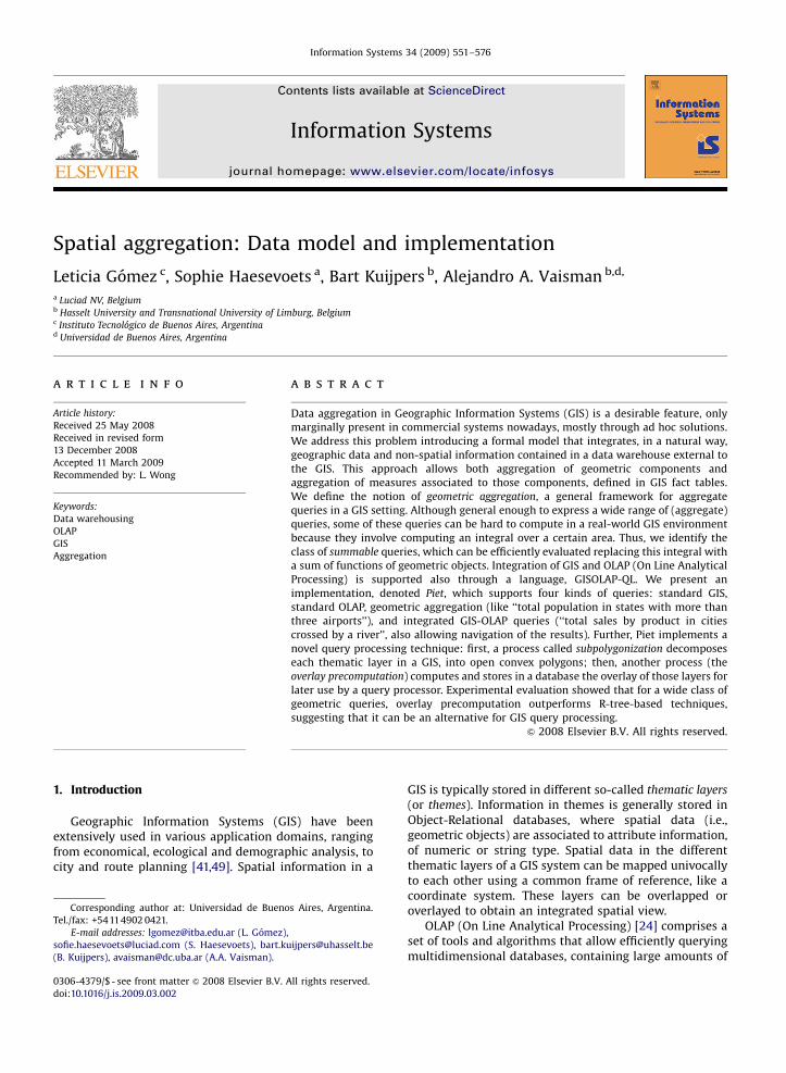
Fig. 1. An example of a GIS dimension schema.


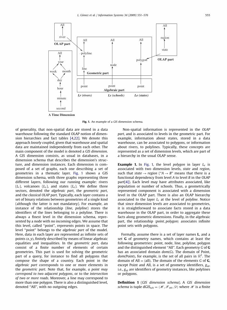
of generality, that non-spatial data are stored in a datawarehouse following the standard OLAP notion of dimen-sion hierarchies and fact tables [4,22]. We denote thisapproach loosely coupled, given that warehouse and spatialdata are maintained independently from each other. Themain component of the model is denoted a GIS dimension.A GIS dimension consists, as usual in databases, in adimension schema that describes the dimension’s struc-ture, and dimension instances. Each dimension is com-posed of a set of graphs, each one describing a set ofgeometries in a thematic layer. Fig. 1 shows a GISdimension schema, with three graphs representing threedifferent layers, following our running example: rivers(Lr), volcanoes (Lv), and states (Le). We define threesectors, denoted the algebraic part, the geometric part,and the classical OLAP part. Typically, each layer contains aset of binary relations between geometries of a single kind(although the latter is not mandatory). For example, aninstance of the relationship (line, polyline) stores theidentifiers of the lines belonging to a polyline. There isalways a finest level in the dimension schema, repre-sented by a node with no incoming edges. We assume thatthis level, called ‘‘point’’, represents points in space. Thelevel ‘‘point’’ belongs to the algebraic part of the model.Here, data in each layer are represented as infinite sets ofpoints ðx; yÞ, finitely described by means of linear algebraicequalities and inequalities. In the geometric part, dataconsist of a finite number of elements of certaingeometries. This part is used for solving the geometricpart of a query, for instance to find all polygons thatcompose the shape of a country. Each point in thealgebraic part corresponds to one or more elements inthe geometric part. Note that, for example, a point may

correspond to two adjacent polygons, or to the intersection

of two or more roads. Moreover, a line may correspond tomore than one polygon. There is also a distinguished level,denoted ‘‘All’’, with no outgoing edges.

Non-spatial information is represented in the OLAP

part, and is associated to levels in the geometric part. Forexample, information about states, stored in a datawarehouse, can be associated to polygons, or informationabout rivers, to polylines. Typically, these concepts arerepresented as a set of dimension levels, which are part ofa hierarchy in the usual OLAP sense.

Example 1. In Fig. 1, the level polygon in layer Le isassociated with two dimension levels, state and region,such that state! region (‘‘A! B’’ means that there is afunctional dependency from level A to level B in the OLAPpart[4]). Each level may have attributes associated, likepopulation or number of schools. Thus, a geometricallyrepresented component is associated with a dimensionlevel in the OLAP part. There is also an OLAP hierarchyassociated to the layer Lr at the level of polyline. Noticethat since dimension levels are associated to geometries,it is straightforward to associate facts stored in a datawarehouse in the OLAP part, in order to aggregate thesefacts along geometric dimensions. Finally, in the algebraicpart, the relationship hpoint; polygoni associates infinitepoint sets with polygons.

Formally, assume there is a set of layer names L, and aset G of geometry names, which contains at least thefollowing geometries: point, node, line, polyline, polygonand the distinguished element ‘‘All’’. Each geometry G of Ghas an associated domain domðGÞ. The domain of Point,domðPointÞ, for example, is the set of all pairs in R2. Thedomain of All ¼ fallg. The domain of the elements G of G,except Point and All, is a set of geometry identifiers, gid,i.e., gid are identifiers of geometry instances, like polylinesor polygons.

Definition 1 (GIS dimension schema). A GIS dimension

schema is tuple dGISsch ¼ hH;Fatt ;Di where H is a finite

ARTICLE IN PRESS

all

x1,y1

x2,y2

x3,y3

x4,y4

l1l2

pl1

Layer Lr

Colorado

r (Lr, line, polyline, lid, plid)

ralg (Lr, line, x, y, lid)

α (Lr, Rivers, Ri, polyline, ’Colorado’)

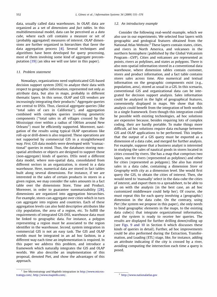
Fig. 2. A portion of a GIS dimension instance in Fig. 1.


set of graphs, Fatt a set of functions, and D a set of OLAPdimension schemas. We define these sets below.

Given a layer L 2 L, HðLÞ, is a graph where: (a) there is a

node for each kind of geometry G 2 G in L; (b) there is an

edge between two nodes Gi and Gj if Gj is composed of

geometries of type Gi (i.e., the granularity of Gj is coarser

than that of Gi); (c) there is a distinguished member All

that has no outgoing edges; (d) there is exactly one node

representing the geometry hpointi with no incoming

edges. The dimension schemas D 2 D are tuples of the

form hdname; Levels;�i , such that dname is the name of

the dimension, Levels is a set of dimension level

names, and � is a partial order between levels (see

[22]). Finally, Fatt contains partial functions (denoted Att)

mapping attributes in OLAP dimensions to geometries in

the layers.

Example 2. The GIS dimension depicted in Fig. 1 has theschema: dGISsch ¼ hfðH1ðLrÞ, ðH2ðLvÞ, H3ðLeÞg, fAttðstateÞ,AttðriverÞ, fRivers; Statesgi. In this schema, for example,H1ðLrÞ ¼ ðfpoint, line, polyline;Allg, fðpoint; lineÞ, ðline,polylineÞ, ðpolyline;AllÞgÞ. For the OLAP dimensionsRivers and States, the Att functions in Fatt are:Attðstate; StatesÞ ¼ ðpolygon; LeÞ (meaning that the attri-bute states maps to polygons in layer Le), and Attðriver,RiversÞ ¼ ðpolyline; LrÞ (i.e., the attribute river maps topolylines in the layer Lr).

Definition 2 (GIS dimension instance). Let dGISsch ¼

hH;Fatt ;Di be a GIS dimension schema. A GIS dimension

instance is a tuple hdGISsch; ralg ; r;a; Dinsti; where (a) ralg isa 5-ary relation representing the rollup between thealgebraic and geometric parts. Thus, it is of the formhLi;Gj; x; y; gidi; where Li is a layer name, Gj is the geometryin the geometric part to which point rolls up, x; y are thecoordinates of a point, and gid is the identifier of the objectassociated to x; y in the geometric part; (b) r is a 5-ary

relation representing the rollup between objects in thegeometric part. It is of the form hLi;Gi;Gj; gidi

; gidji;where Li

is a layer name, Gi and Gj are geometries in the geometricpart such that the former rolls up to the latter (i.e., there isan edge Gi ! Gj in HðLiÞ in dGISsch), and gidi

and gidjare

instances of these geometries. We denote ralg and r rollup

relations. The function a maps a member in a level level inan OLAP dimension D; to an object gid in a geometry G in alayer L: This mapping corresponds to the functions in Fatt :

Intuitively, a provides a link between a data warehouseinstance and an instance of the hierarchy graph. Finally,for each dimension schema D 2 D there is a dimensioninstance in Dinst , composed of a set of rollup functions[22] that relate elements in the different dimension levels(intuitively, these functions indicate how dimension levelmembers are aggregated).

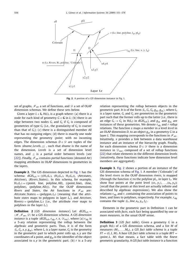
Example 3. Fig. 2 shows a portion of an instance of theGIS dimension schema of Fig. 1. A member (‘Colorado’) ofthe level rivers in the OLAP dimension rivers, is mapped(through the function a) to the polyline pl1; in layer Lr. Weshow four points at the point level fðx1; y1Þ; . . . ; ðx4; y4Þg

(recall that the points at this level are actually infinite anddescribed by algebraic expressions). We also show therelations ralg and r; containing the association of points tolines, and lines to polylines, respectively. For example, ralg

contains the tuple hLr ; line; x4; y4; l2i.

Elements in the geometric part in Definition 1 can beassociated with facts, each fact being quantified by one ormore measures, in the usual OLAP sense.

Definition 3 (GIS fact table). Given a geometry G in agraph HðLÞ of a GIS dimension schema, and a list M ofmeasures ðM1; . . . ;MkÞ; a GIS fact table schema is a tupleFT ¼ ðG; L;MÞ. A base GIS fact table schema is a tuple BFT ¼

ðpoint; L; MÞ that means, a fact table with the finestgeometric granularity. A GIS fact table instance is a function

ARTICLE IN PRESS


ft mapping values in domðGÞ � L to values in domðM1Þ �

� � � � domðMkÞ: A base GIS fact table instance maps values inR2� L to values in domðM1Þ � � � � � domðMkÞ:

Example 4. Consider a fact table containing state popula-tions in our running example, stored at the polygon level.The fact table schema would be ðpolyId; Le; populationÞ;

where population is the measure. If information about, forexample, temperature data, is stored at the point level, wewould have a base fact table with schema ðpoint;

Le; temperatureÞ; with instances like ðx1; y1; Le;25Þ: Notethat temporal information could be also stored in thesefact tables, by simply adding the time dimension to thefact table. This would allow to store temperatureinformation across time.

Basically, a GIS fact table is a standard OLAP fact tablewhere one of the dimensions is composed of geometricobjects in a layer. Classical fact tables in the OLAP part,defined in terms of the OLAP dimension schemas can alsoexist. For instance, instead of storing the populationassociated to a polygon identifier, as in Example 4, thisinformation may reside in a data warehouse.

3.1. Geometric aggregation

We now give a precise definition of the kinds ofaggregate queries we deal with.

Definition 4 (Geometric aggregation). Given a GIS dimen-sion as introduced in Definitions 1 and 2, a geometric

aggregation is the expressionZZ

R2dCðx; yÞhðx; yÞdx dy,

where C ¼ fðx; yÞ 2 R2j jðx; yÞg,7 and dC is defined as

follows:

dCðx; yÞ ¼ 1 on the two-dimensional parts of C is a Dirac

delta function [8] on the zero-dimensional parts of C; and it

is the product of a Dirac delta function with a combination

of Heaviside step functions [21] for the one-dimensional

parts of C (see Appendix A for details). Also, j is a first-

order (FO) formula in a multi-sorted logic L over the

reals, geometric objects, and dimension level members.

The vocabulary of L contains the relations r; ralg ; and the

function a, together with the binary functions þ and � on

real numbers, the binary predicate o on real numbers and

the real constants 0 and 1.8 Also constants for layers,

dimension names, dimension level names, and geometry

names may appear in L.9 Atomic formulas in L are

combined with the standard logical operators^, _ and :

7 The sets C in Definition 4 are known in mathematics as semi-

algebraic sets. In the GIS practice, only linear sets (points, polylines and

polygons) are used. Therefore, it could suffice to work with addition over

the reals only, leaving out multiplication.8 The FO logic over the structure ðR;þ;�;o;0;1Þ is well-known as

the FO logic with polynomial constraints over the reals. This logic is well-

studied as a data model and query language in the field of constraint

databases [37].9 We may also quantify over layer variables, dimension level

variables, etc., but we have chosen not to do this, for the sake of clarity.

and existential and universal quantifiers over real vari-

ables, variables for geometric objects identifiers, and

variables for dimension level members. Finally, h is an

integrable function constructed from elements of f1; ftg (ft

stands for fact table), using arithmetic operations.

Note that this definition gives the basic construct for

geometric aggregation queries. More involved queries can

be written as combinations of this construct (e.g., ‘‘total

number of airports per square kilometer’’ would require

dividing the geometric aggregation that computes the

number of airports in the query region, by the aggregation

computing the area of such region).10

Example 5. The following queries refer to the exampleintroduced in Section 1. The layers containing cities andrivers are labeled Lc and Lr ; respectively, although in orderto make the queries more interesting, we define cities aspolygons instead of points. The population density foreach coordinate in Lc is stored in a base fact table ftpop (weassume it is stored in some finite way, i.e., usingpolynomial equations over the real numbers). In whatfollows, we abbreviate Point, Polygon and PolyLine by Pt,Pg and Pl, respectively. Also, Ci and Ri stand for theattributes city and river; respectively. Further, all con-stants are capitalized, to distinguish them from variablesin our expressions. Finally, note that in the queries below,the Dirac delta function is such that dCðx; yÞ ¼ 1; inside theregion C; and dCðx; yÞ ¼ 0; outside this region.

Q1: Total population of cities within 100 km from San

Francisco:

Q1 �

ZZC1

ftpopðx; y; LcÞdx dy,

where C1 is defined by the expression:

C1 ¼ fðx; yÞ 2 R2jð9x0Þð9y0Þð9x00Þð9y00Þð9pg1Þð9pg2Þð9cÞ

ðaðLc ;Cities;Ci;Pg; San FranciscoÞ

¼ pg1 ^ ralgðLc;Pg; x0; y0; pg1Þ ^ aðLc ;Cities;Ci;Pg; cÞ

¼ pg2 ^ ralgðLc;Pg; x00; y00; pg2Þ ^ pg2apg1 ^ ððx00 � x0Þ2

þ ðy00 � y0Þ2p1002Þ ^ ralgðLc ;Pg; x; y; pg2ÞÞg.

Here, aðLc;Cities;Ci;Pg; San FranciscoÞ maps the city of

San Francisco (an instance of the level Ci in dimension

Cities), to a polygon pg1 in layer Lc. The third and fourth

lines find the cities within 100 km of San Francisco, and

the relation ralgðLc;Pg; x; y; pg2Þ;with the mapping between

the points and the polygons that satisfy the condition. We

are interested in the points that belong to pg2:

Q2: Total population of the cities crossed by the

Colorado river:

Q2 �

ZZC2

ftpopðx; y; LcÞdx dy,

10 For the language L; as usual in relational database theory, we

assume set semantics, while in Section 8, set, bag, and mixed bag-set

semantics [6] are supported through the SQL-like query languages.

ARTICLE IN PRESS

11 This can be extended to support bag semantics [13,25], at the


C2 ¼ fðx; yÞ 2 R2jð9x0Þð9y0Þð9pg1Þð9cÞ

ðralgðLc ;Pl; x0; y0;aðLr ;Rivers;Ri;Pl;ColoradoÞÞ

^ aðLc ;Cities;Ci;Pg; cÞ ¼ pg1 ^ ralgðLc ;Pg; x0; y0; pg1Þ

^ ralgðLc ;Pg; x; y; pg1ÞÞg.

4. Summable queries

The framework we presented in the previous section isgeneral enough to allow expressing complex geometricaggregation queries (Definition 4) over a GIS in a formalway. However, computing these queries within thisframework can be extremely costly, as the followingdiscussion shows. Let us consider again Example 5. Hereftpop is a density function. This could be a constantfunction over cities, e.g., the density in all points of SanFrancisco, say, 1000 people per square kilometer. But ftpop

is allowed to be more complex too, like for instance apiecewise constant density function or even a veryprecise function describing the true density at any point.Moreover, just computing the expression ‘‘C’’ of Definition4 could be practically infeasible. In Example 5, queryQ2; computing on-the-fly the intersection (overlay)of the cities and rivers is likely to be very expensive.Therefore, we identify a subclass of geometric aggregatequeries that simplifies the computation of the integral ofthe functions hðx; yÞ of Definition 4. Specifically, we showthat storing less precise information (for instance, havinga simpler function ftpop in Example 5) results in a moreefficient computation of the integral. There are querieswhere even if the function ftpop is piecewise constant overthe cities, there is no other way of computing thepopulation over the region defined by j than taking theintegral, as j can define any semi-algebraic set. Anexample of a query of this kind is: ‘‘Total populationendangered by a poisonous cloud described by j; aformula in FO logic over ðR;þ;�;o;0;1Þ)’’. Further, justcomputing the population within an arbitrarily givenregion cannot be performed. However, for queries Q1 andQ2 the situation is different. Indeed, the sets C1 and C2

return a finite set of polygons, representing cities. If thefunction ftpop is constant for each city, it suffices tocompute ftpop once for each polygon, and then multiplythis value with the area of the polygon. Summing up theproducts would yield the correct result, without the needof integrating ftpop over the area C1 or C2. This is exactlythe subclass of queries we want to propose, those that canbe rewritten as sums of functions of geometric objectsreturned by condition ‘‘C’’. We denote these queriessummable.

Definition 5 (Summable query). A geometric aggregationquery Q ¼

RRR2dCðx; yÞhðx; yÞdx dy is summable if and only

if:

expense of increasing the presentation formal overload, and we chose to

avoid this. Moreover, queries requiring bag semantics, like ‘‘Total number
(1) of rivers in California and Nevada’’ (where, if a river crosses both states
must be counted twice), can be written using combinations of the basic

construct (splitting the query and adding the results), as we commented

in Section 3.1.

C ¼S

g2G extðgÞ; where G is a set of geometric objects,and extðgÞ means the geometric extension of g, that is,the subset of R2 that g occupies (e.g., a polygon or apolyline, as a subset of R2).

(2)
There exists h0; constructed using f1; f tg and arith-metic operators, such that
Q ¼Xg2S

h0ðgÞ with h0ðgÞ ¼

ZZR2dextðgÞðx; yÞhðx; yÞdx dy.

Working with less accurate functions for this type ofqueries means that the base GIS fact table instances ofDefinition 3 will be defined as mappings from values indomðGÞ � L to values in domðM1Þ � � � � � domðMkÞ (wherethe elements in domðGÞ are the geometric objects g 2 G

such that ralgðL;G; x; y; gÞÞ; instead of mappings from valuesin R2

� L to values in domðM1Þ � � � � � domðMkÞ:

Note that Definition 5 implies that the three summar-izability conditions defined by Lenz et al. [28] must bepreserved. The first two conditions (disjointness ofcategorical attributes, and completeness, respectively)are satisfied by our definition of a GIS dimension. Thethird condition requires function h0ðgÞ to be summarizableover g: The functions we use in this paper (typically sums,averages and maximum/minimum) satisfy the thirdcondition in [28]. We remark that in this section (like inthe previous one) we work with set semantics. Since theintegration region is replaced by geometric identifiers, setsemantics expresses correctly the most usual summablequeries of interest.11

Example 6. Let us reconsider query Q2 from Example 5.The function ftpop (i.e., the fact table) now maps elementsof domðPolygonÞ to populations. Note that C02returns afinite set of polygons, indicated by their ids (denoted gid).

Q2: Total population of the cities crossed by the Colorado

river:

Q2 �X

gid2C02

ftpopðgid; LcÞ.

C02 ¼ fgidjð9xÞð9yÞð9cÞ

ðralgðLr ;Pl; x; y;aðLr ;Rivers;Ri;Pl;ColoradoÞÞ

^ aðLc ;Cities;Ci;Pg; cÞ ¼ gid ^ ralgðLc ;Pg; x; y; gidÞÞg.

Queries aggregating over zero or one-dimensionalregions (like, for instance, queries requiring counting thenumber of occurrences of some phenomena) can also besummable. For example, counting the number of airportsover a certain region, can be expressed as Q �

Pgid2C1:

Moreover, the aggregation can also be expressed over afact table in the application part of the model, like in thequery ‘‘Total number of students in cities crossed by theColorado river’’. This query is expressed asP

Ci2C0 ft#studentscities ðCiÞ; where the sum is performed over a

set of city identifiers (the integration region C0, which we

ARTICLE IN PRESS

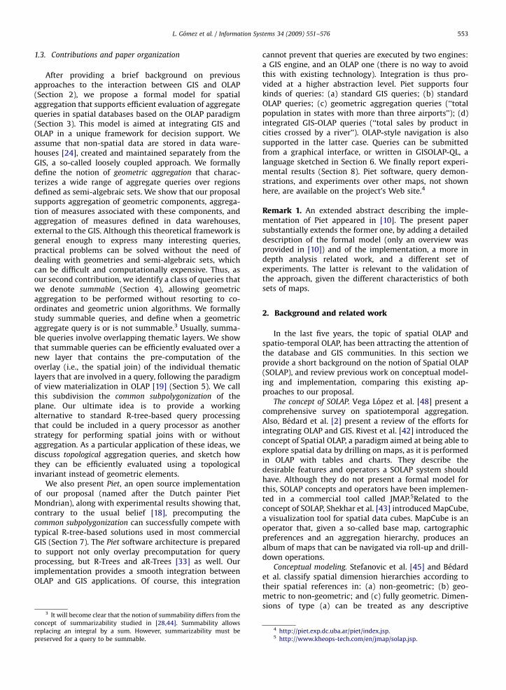
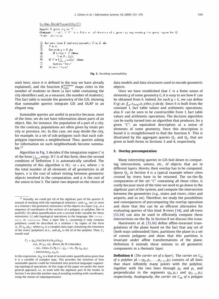
Fig. 3. Deciding summability.


omit here, since it is defined in the way we have alreadyexplained), and the function ft#students

cities maps cities to thenumber of students in them (a fact table containing thecity identifiers and, as a measure, the number of students).This fact table is outside the geometry of the GIS, showingthat summable queries integrate GIS and OLAP in anelegant way.

Summable queries are useful in practice because, mostof the time, we do not have information about parts of anobject, like, for instance, the population of a part of a city.On the contrary, populations are often given by totals percity or province, etc. In this case, we may divide the city,for example, in a set of sub-polygons such that each sub-polygon represents a neighborhood. Thus, queries askingfor information on such neighborhoods become summa-ble.12

Algorithm in Fig. 3 decides if the integration region C isof the form

Sg2G extðgÞ: If C is of this form, then the second

condition of Definition 5 is automatically satisfied. Thecomplexity of this algorithm is Oðg � ðsþcÞÞ; where g isthe total number of all elements of all geometries in alllayers, s is the cost of subset testing between geometricobjects involved in the computation, and c is the cost ofthe union in line 5. The latter two depend on the choice of

12 Actually, we could get rid of the algebraic part of the queries if,

instead of working with the topological relations r and ralg ; we (a) store

in a relation r the geometric extension e of the objects in a layer (e.g., as a

sequence of coordinates of the vertices of a polygon, or polyline, like in

postGIS); (b) allow quantification over a second-order variable for these

extensions; (c) add topological operations to the language, like inter-

sect, or contains. Thus, a layer like Lr (assuming it only contains

polylines) could be described in a relation r by tuples of the form

hLr ; Pl; epl; plidi; where epl is a complex data type containing the extension

of the rivers (polylines) in Lr ; and plid is the id of the polyline. Then, C02would read

C02 ¼ fgidjð9xÞð9yÞð9cÞð9eplÞð9epg Þ

ðrðLr ;Pl; epl;aðLr ;Rivers;Ri; Pl;ColoradoÞÞ

^ aðLc ;Cities;Ci; Pg; cÞ ¼ gid ^ rðLc ;Pg; epg ; gidÞ

^ intersectsðepl; epg ÞÞg.

In this expression, 9epg is a kind of second-order quantification given that

it is a variable of complex type. This provides the intuition of how

summable queries could be translated into practical languages support-

ing topological operations. At this stage of the paper we prefer the more

general approach, i.e., to work with the algebraic part of the model. In

Section 5 we describe another way of avoiding working with coordinates,

using the notion of subpolygonization.

data models and data structures used to encode geometricobjects.

Once we have established that C is a finite union ofelements g of some geometry G, it is easy to see how h0 canbe obtained from h. Indeed, for each g 2 G, we can defineh0ðgÞ as

RRR2dextðgÞðx; yÞhðx; yÞdx dy. Since h is built from the

constant 1, fact table values and arithmetic operations,also h0 can be seen to be constructible from 1, fact tablevalues and arithmetic operations. The decision algorithmcan be easily turned into an algorithm that produces, for agiven ‘‘C’’, an equivalent description as a union ofelements of some geometry. Once this description isfound it is straightforward to find the function h0: This isillustrated by the aggregate queries Q1 and Q2 that aregiven in both forms in Sections 3 and 4, respectively.

5. Overlay precomputation

Many interesting queries in GIS boil down to comput-ing intersections, unions, etc., of objects that are indifferent layers. Hereto, their overlay has to be computed.Query Q2 in Section 4 is a typical example where citiescrossed by rivers have to be returned. The on-the-flycomputation of the set ‘‘C’’ containing all those cities, iscostly because most of the time we need to go down to thealgebraic part of the system, and compute the intersectionbetween the geometries (e.g., states and rivers, cities andairports, and so on). Therefore, we study the possibilitiesand consequences of precomputing the overlay operationand show that this can be an efficient alternative forevaluating queries of this kind. R-trees [14], and aR-trees[33,34] can also be used to efficiently compute theseintersections on-the-fly. In Section 8 we discuss this issue.

Haesevoets et al. [15,16] define affine-invariant trian-gulations of the plane based on the fact that any set of(both ways unbounded) lines, partitions the plane in a setof convex polygons and show that this partition isinvariant under affine transformations of the plane.Definition 6 extends these notions to all geometriccomponents in a thematic layer.

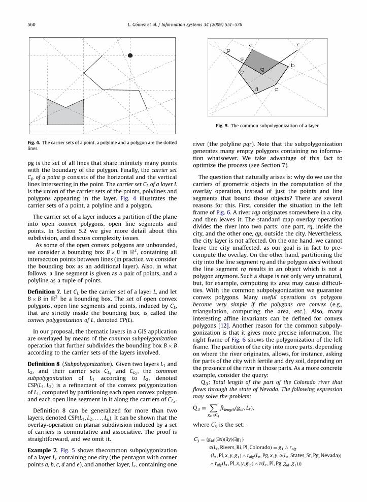
Definition 6 (The carrier set of a layer). The carrier set Cpl

of a polyline pl ¼ ðp0; p1; . . . ; pðl�1Þ; plÞ consists of all linesthat share infinitely many points with the polyline,together with the two lines through p0 and pl; andperpendicular to the segments ðp0; p1Þ and ðpðl�1Þ; plÞ,respectively. Analogously, the carrier set Cpg of a polygon

ARTICLE IN PRESS

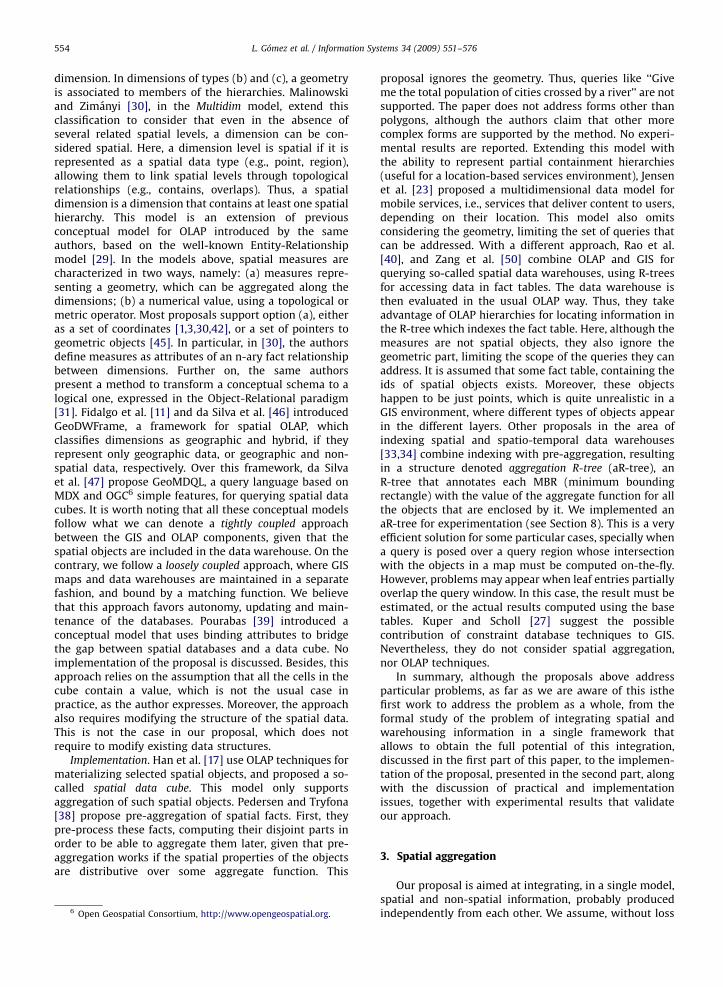
Fig. 4. The carrier sets of a point, a polyline and a polygon are the dotted

lines.

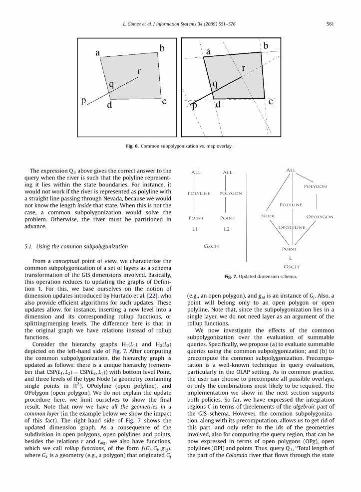
Fig. 5. The common subpolygonization of a layer.


pg is the set of all lines that share infinitely many pointswith the boundary of the polygon. Finally, the carrier set

Cp of a point p consists of the horizontal and the verticallines intersecting in the point. The carrier set CL of a layer L

is the union of the carrier sets of the points, polylines andpolygons appearing in the layer. Fig. 4 illustrates thecarrier sets of a point, a polyline and a polygon.

The carrier set of a layer induces a partition of the planeinto open convex polygons, open line segments andpoints. In Section 5.2 we give more detail about thissubdivision, and discuss complexity issues.

As some of the open convex polygons are unbounded,we consider a bounding box B� B in R2, containing allintersection points between lines (in practice, we considerthe bounding box as an additional layer). Also, in whatfollows, a line segment is given as a pair of points, and apolyline as a tuple of points.

Definition 7. Let CL be the carrier set of a layer L, and letB� B in R2 be a bounding box. The set of open convexpolygons, open line segments and points, induced by CL,that are strictly inside the bounding box, is called theconvex polygonization of L, denoted CPðLÞ.

In our proposal, the thematic layers in a GIS applicationare overlayed by means of the common subpolygonization

operation that further subdivides the bounding box B� B

according to the carrier sets of the layers involved.

Definition 8 (Subpolygonization). Given two layers L1 andL2; and their carrier sets CL1

and CL2; the common

subpolygonization of L1 according to L2, denotedCSPðL1; L2Þ is a refinement of the convex polygonizationof L1, computed by partitioning each open convex polygonand each open line segment in it along the carriers of CL2

.

Definition 8 can be generalized for more than twolayers, denoted CSPðL1; L2; . . . ; LkÞ: It can be shown that theoverlay-operation on planar subdivision induced by a setof carriers is commutative and associative. The proof isstraightforward, and we omit it.

Example 7. Fig. 5 shows thecommon subpolygonizationof a layer Lc containing one city (the pentagon with cornerpoints a, b, c, d and e), and another layer, Lr , containing one

river (the polyline pqr). Note that the subpolygonizationgenerates many empty polygons containing no informa-tion whatsoever. We take advantage of this fact tooptimize the process (see Section 7).

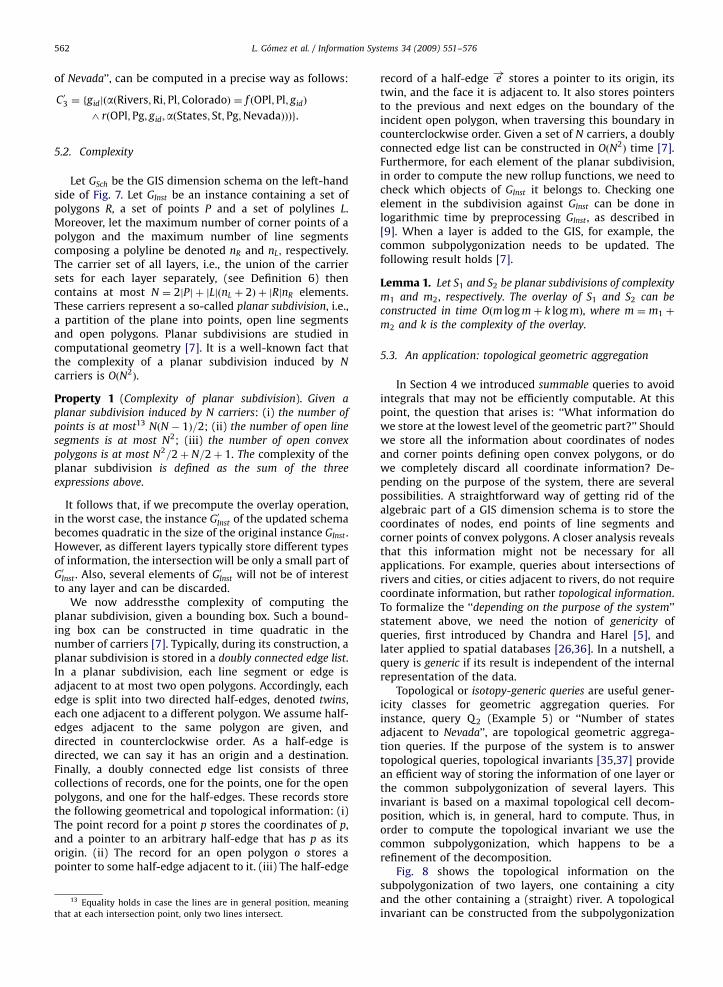
The question that naturally arises is: why do we use thecarriers of geometric objects in the computation of theoverlay operation, instead of just the points and linesegments that bound those objects? There are severalreasons for this. First, consider the situation in the leftframe of Fig. 6. A river rqp originates somewhere in a city,and then leaves it. The standard map overlay operationdivides the river into two parts: one part, rq, inside thecity, and the other one, qp, outside the city. Nevertheless,the city layer is not affected. On the one hand, we cannotleave the city unaffected, as our goal is in fact to pre-compute the overlay. On the other hand, partitioning thecity into the line segment rq and the polygon abcd withoutthe line segment rq results in an object which is not apolygon anymore. Such a shape is not only very unnatural,but, for example, computing its area may cause difficul-ties. With the common subpolygonization we guaranteeconvex polygons. Many useful operations on polygons

become very simple if the polygons are convex (e.g.,triangulation, computing the area, etc.). Also, manyinteresting affine invariants can be defined for convexpolygons [12]. Another reason for the common subpoly-gonization is that it gives more precise information. Theright frame of Fig. 6 shows the polygonization of the leftframe. The partition of the city into more parts, dependingon where the river originates, allows, for instance, askingfor parts of the city with fertile and dry soil, depending onthe presence of the river in those parts. As a more concreteexample, consider the query:

Q3: Total length of the part of the Colorado river that

flows through the state of Nevada. The following expression

may solve the problem:

Q3 �X

gid2C04

ftlengthðgid; LrÞ,

where C03 is the set:

C03 ¼ fgidjð9xÞð9yÞð9g1Þ

aðLr ;Rivers;Ri;Pl;ColoradoÞ ¼ g1 ^ ralg

ðLr ;Pl; x; y; g1Þ ^ ralgðLe;Pg; x; y;aðLe; States; St;Pg;NevadaÞÞ

^ ralgðLr ;Pl; x; y; gidÞ ^ rðLr ;Pl;Pg; gid; g1ÞÞg

ARTICLE IN PRESS

Fig. 6. Common subpolygonization vs. map overlay.


The expression Q3 above gives the correct answer to thequery when the river is such that the polyline represent-ing it lies within the state boundaries. For instance, itwould not work if the river is represented as polyline witha straight line passing through Nevada, because we wouldnot know the length inside that state. When this is not thecase, a common subpolygonization would solve theproblem. Otherwise, the river must be partitioned inadvance.

Fig. 7. Updated dimension schema.

5.1. Using the common subpolygonization

From a conceptual point of view, we characterize thecommon subpolygonization of a set of layers as a schematransformation of the GIS dimensions involved. Basically,this operation reduces to updating the graphs of Defini-tion 1. For this, we base ourselves on the notion ofdimension updates introduced by Hurtado et al. [22], whoalso provide efficient algorithms for such updates. Theseupdates allow, for instance, inserting a new level into adimension and its corresponding rollup functions, orsplitting/merging levels. The difference here is that inthe original graph we have relations instead of rollupfunctions.

Consider the hierarchy graphs H1ðL1Þ and H2ðL2Þ

depicted on the left-hand side of Fig. 7. After computingthe common subpolygonization, the hierarchy graph isupdated as follows: there is a unique hierarchy (remem-ber that CSPðL1; L2Þ ¼ CSPðL2; L1Þ) with bottom level Point,and three levels of the type Node (a geometry containingsingle points in R2), OPolyline (open polyline), andOPolygon (open polygon). We do not explain the updateprocedure here, we limit ourselves to show the finalresult. Note that now we have all the geometries in a

common layer (in the example below we show the impactof this fact). The right-hand side of Fig. 7 shows theupdated dimension graph. As a consequence of thesubdivision in open polygons, open polylines and points,besides the relations r and ralg ; we also have functions,which we call rollup functions, of the form f ðGj;Gk; gidÞ;

where Gk is a geometry (e.g., a polygon) that originated Gj

(e.g., an open polygon), and gid is an instance of Gj. Also, apoint will belong only to an open polygon or openpolyline. Note that, since the subpolygonization lies in asingle layer, we do not need layer as an argument of therollup functions.

We now investigate the effects of the commonsubpolygonization over the evaluation of summablequeries. Specifically, we propose (a) to evaluate summablequeries using the common subpolygonization; and (b) toprecompute the common subpolygonization. Precompu-tation is a well-known technique in query evaluation,particularly in the OLAP setting. As in common practice,the user can choose to precompute all possible overlays,or only the combinations most likely to be required. Theimplementation we show in the next section supportsboth policies. So far, we have expressed the integrationregions C in terms of theelements of the algebraic part ofthe GIS schema. However, the common subpolygoniza-tion, along with its precomputation, allows us to get rid ofthis part, and only refer to the ids of the geometriesinvolved, also for computing the query region, that can benow expressed in terms of open polygons (OPg), openpolylines (OPl) and points. Thus, query Q3, ‘‘Total length ofthe part of the Colorado river that flows through the state

ARTICLE IN PRESS


of Nevada’’, can be computed in a precise way as follows:

C03 ¼ fgidjðaðRivers;Ri;Pl;ColoradoÞ ¼ f ðOPl;Pl; gidÞ

^ rðOPl;Pg; gid;aðStates; St;Pg;NevadaÞÞÞg.

5.2. Complexity

Let GSch be the GIS dimension schema on the left-handside of Fig. 7. Let GInst be an instance containing a set ofpolygons R, a set of points P and a set of polylines L.Moreover, let the maximum number of corner points of apolygon and the maximum number of line segmentscomposing a polyline be denoted nR and nL; respectively.The carrier set of all layers, i.e., the union of the carriersets for each layer separately, (see Definition 6) thencontains at most N ¼ 2jPj þ jLjðnL þ 2Þ þ jRjnR elements.These carriers represent a so-called planar subdivision, i.e.,a partition of the plane into points, open line segmentsand open polygons. Planar subdivisions are studied incomputational geometry [7]. It is a well-known fact thatthe complexity of a planar subdivision induced by N

carriers is OðN2Þ.

Property 1 (Complexity of planar subdivision). Given a

planar subdivision induced by N carriers: (i) the number of

points is at most13 NðN � 1Þ=2; (ii) the number of open line

segments is at most N2; (iii) the number of open convex

polygons is at most N2=2þ N=2þ 1. The complexity of theplanar subdivision is defined as the sum of the three

expressions above.

It follows that, if we precompute the overlay operation,in the worst case, the instance G0Inst of the updated schemabecomes quadratic in the size of the original instance GInst .However, as different layers typically store different typesof information, the intersection will be only a small part ofG0Inst . Also, several elements of G0Inst will not be of interestto any layer and can be discarded.

We now addressthe complexity of computing theplanar subdivision, given a bounding box. Such a bound-ing box can be constructed in time quadratic in thenumber of carriers [7]. Typically, during its construction, aplanar subdivision is stored in a doubly connected edge list.In a planar subdivision, each line segment or edge isadjacent to at most two open polygons. Accordingly, eachedge is split into two directed half-edges, denoted twins,each one adjacent to a different polygon. We assume half-edges adjacent to the same polygon are given, anddirected in counterclockwise order. As a half-edge isdirected, we can say it has an origin and a destination.Finally, a doubly connected edge list consists of threecollections of records, one for the points, one for the openpolygons, and one for the half-edges. These records storethe following geometrical and topological information: (i)The point record for a point p stores the coordinates of p,and a pointer to an arbitrary half-edge that has p as itsorigin. (ii) The record for an open polygon o stores apointer to some half-edge adjacent to it. (iii) The half-edge

13 Equality holds in case the lines are in general position, meaning

that at each intersection point, only two lines intersect.

record of a half-edge e!

stores a pointer to its origin, itstwin, and the face it is adjacent to. It also stores pointersto the previous and next edges on the boundary of theincident open polygon, when traversing this boundary incounterclockwise order. Given a set of N carriers, a doublyconnected edge list can be constructed in OðN2

Þ time [7].Furthermore, for each element of the planar subdivision,in order to compute the new rollup functions, we need tocheck which objects of GInst it belongs to. Checking oneelement in the subdivision against GInst can be done inlogarithmic time by preprocessing GInst , as described in[9]. When a layer is added to the GIS, for example, thecommon subpolygonization needs to be updated. Thefollowing result holds [7].

Lemma 1. Let S1 and S2 be planar subdivisions of complexity

m1 and m2, respectively. The overlay of S1 and S2 can be

constructed in time Oðm log mþ k log mÞ, where m ¼ m1 þ

m2 and k is the complexity of the overlay.

5.3. An application: topological geometric aggregation

In Section 4 we introduced summable queries to avoidintegrals that may not be efficiently computable. At thispoint, the question that arises is: ‘‘What information dowe store at the lowest level of the geometric part?’’ Shouldwe store all the information about coordinates of nodesand corner points defining open convex polygons, or dowe completely discard all coordinate information? De-pending on the purpose of the system, there are severalpossibilities. A straightforward way of getting rid of thealgebraic part of a GIS dimension schema is to store thecoordinates of nodes, end points of line segments andcorner points of convex polygons. A closer analysis revealsthat this information might not be necessary for allapplications. For example, queries about intersections ofrivers and cities, or cities adjacent to rivers, do not requirecoordinate information, but rather topological information.To formalize the ‘‘depending on the purpose of the system’’statement above, we need the notion of genericity ofqueries, first introduced by Chandra and Harel [5], andlater applied to spatial databases [26,36]. In a nutshell, aquery is generic if its result is independent of the internalrepresentation of the data.

Topological or isotopy-generic queries are useful gener-icity classes for geometric aggregation queries. Forinstance, query Q2 (Example 5) or ‘‘Number of statesadjacent to Nevada’’, are topological geometric aggrega-tion queries. If the purpose of the system is to answertopological queries, topological invariants [35,37] providean efficient way of storing the information of one layer orthe common subpolygonization of several layers. Thisinvariant is based on a maximal topological cell decom-position, which is, in general, hard to compute. Thus, inorder to compute the topological invariant we use thecommon subpolygonization, which happens to be arefinement of the decomposition.

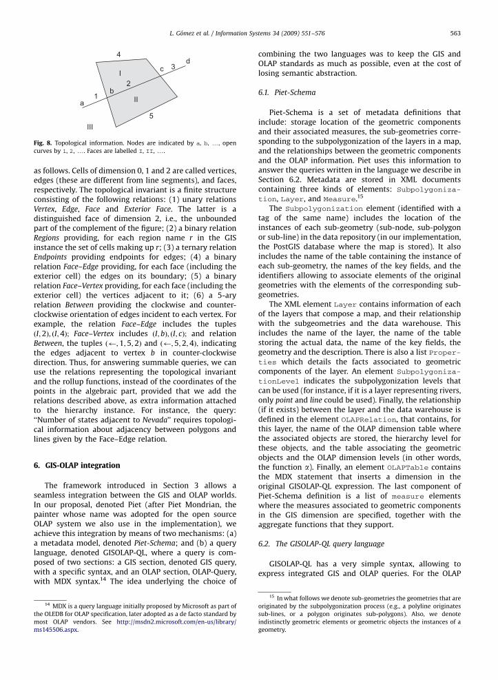
Fig. 8 shows the topological information on thesubpolygonization of two layers, one containing a cityand the other containing a (straight) river. A topologicalinvariant can be constructed from the subpolygonization

ARTICLE IN PRESS

ab

cd

I

II

III

1

2

3

4

5

Fig. 8. Topological information. Nodes are indicated by a, b, y, open

curves by 1, 2, y. Faces are labelled I, II, y.


as follows. Cells of dimension 0, 1 and 2 are called vertices,edges (these are different from line segments), and faces,respectively. The topological invariant is a finite structureconsisting of the following relations: (1) unary relationsVertex, Edge, Face and Exterior Face. The latter is adistinguished face of dimension 2, i.e., the unboundedpart of the complement of the figure; (2) a binary relationRegions providing, for each region name r in the GISinstance the set of cells making up r; (3) a ternary relationEndpoints providing endpoints for edges; (4) a binaryrelation Face–Edge providing, for each face (including theexterior cell) the edges on its boundary; (5) a binaryrelation Face–Vertex providing, for each face (including theexterior cell) the vertices adjacent to it; (6) a 5-aryrelation Between providing the clockwise and counter-clockwise orientation of edges incident to each vertex. Forexample, the relation Face–Edge includes the tuplesðI;2Þ; ðI;4Þ; Face–Vertex includes ðI; bÞ; ðI; cÞ; and relationBetween, the tuples ð ;1;5;2Þ and ð ;5;2;4Þ; indicatingthe edges adjacent to vertex b in counter-clockwisedirection. Thus, for answering summable queries, we canuse the relations representing the topological invariantand the rollup functions, instead of the coordinates of thepoints in the algebraic part, provided that we add therelations described above, as extra information attachedto the hierarchy instance. For instance, the query:‘‘Number of states adjacent to Nevada’’ requires topologi-cal information about adjacency between polygons andlines given by the Face–Edge relation.

6. GIS-OLAP integration

The framework introduced in Section 3 allows aseamless integration between the GIS and OLAP worlds.In our proposal, denoted Piet (after Piet Mondrian, thepainter whose name was adopted for the open sourceOLAP system we also use in the implementation), weachieve this integration by means of two mechanisms: (a)a metadata model, denoted Piet-Schema; and (b) a querylanguage, denoted GISOLAP-QL, where a query is com-posed of two sections: a GIS section, denoted GIS query,with a specific syntax, and an OLAP section, OLAP-Query,with MDX syntax.14 The idea underlying the choice of

14 MDX is a query language initially proposed by Microsoft as part of

the OLEDB for OLAP specification, later adopted as a de facto standard by

most OLAP vendors. See http://msdn2.microsoft.com/en-us/library/

ms145506.aspx.

combining the two languages was to keep the GIS andOLAP standards as much as possible, even at the cost oflosing semantic abstraction.

6.1. Piet-Schema

Piet-Schema is a set of metadata definitions thatinclude: storage location of the geometric componentsand their associated measures, the sub-geometries corre-sponding to the subpolygonization of the layers in a map,and the relationships between the geometric componentsand the OLAP information. Piet uses this information toanswer the queries written in the language we describe inSection 6.2. Metadata are stored in XML documentscontaining three kinds of elements: Subpolygoniza-

tion, Layer, and Measure.15

The Subpolygonization element (identified with atag of the same name) includes the location of theinstances of each sub-geometry (sub-node, sub-polygonor sub-line) in the data repository (in our implementation,the PostGIS database where the map is stored). It alsoincludes the name of the table containing the instance ofeach sub-geometry, the names of the key fields, and theidentifiers allowing to associate elements of the originalgeometries with the elements of the corresponding sub-geometries.

The XML element Layer contains information of eachof the layers that compose a map, and their relationshipwith the subgeometries and the data warehouse. Thisincludes the name of the layer, the name of the tablestoring the actual data, the name of the key fields, thegeometry and the description. There is also a list Proper-ties which details the facts associated to geometriccomponents of the layer. An element Subpolygoniza-

tionLevel indicates the subpolygonization levels thatcan be used (for instance, if it is a layer representing rivers,only point and line could be used). Finally, the relationship(if it exists) between the layer and the data warehouse isdefined in the element OLAPRelation, that contains, forthis layer, the name of the OLAP dimension table wherethe associated objects are stored, the hierarchy level forthese objects, and the table associating the geometricobjects and the OLAP dimension levels (in other words,the function a). Finally, an element OLAPTable containsthe MDX statement that inserts a dimension in theoriginal GISOLAP-QL expression. The last component ofPiet-Schema definition is a list of measure elementswhere the measures associated to geometric componentsin the GIS dimension are specified, together with theaggregate functions that they support.

6.2. The GISOLAP-QL query language

GISOLAP-QL has a very simple syntax, allowing toexpress integrated GIS and OLAP queries. For the OLAP

15 In what follows we denote sub-geometries the geometries that are

originated by the subpolygonization process (e.g., a polyline originates

sub-lines, or a polygon originates sub-polygons). Also, we denote

indistinctly geometric elements or geometric objects the instances of a

geometry.

http://msdn2.microsoft.com/en-us/library/ms145506.aspx

http://msdn2.microsoft.com/en-us/library/ms145506.aspx

ARTICLE IN PRESS


part of the query we keep the syntax and semantics ofMDX. A GISOLAP-QL query is of the form:

wo

GIS-Query j OLAP-Query

A pipe (‘‘j’’) separates two query sections: a GIS queryand an OLAP query. The OLAP section of the query appliesto the OLAP part of the data model (namely, the datawarehouse) and is written in MDX. The GIS part of thequery has the typical SELECT FROM WHERE SQL form,except for a separator (‘‘;’’) at the end of each clause:

SELECT list of layers and/or measures;FROM Piet-Schema;WHERE geometric operations;

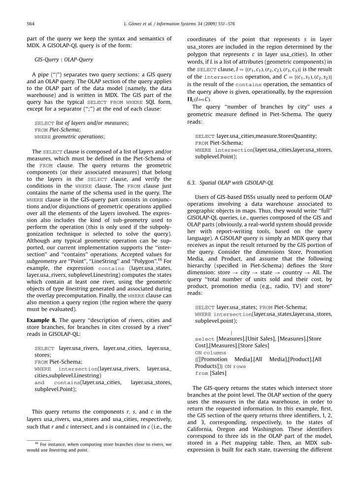
The SELECT clause is composed of a list of layers and/ormeasures, which must be defined in the Piet-Schema ofthe FROM clause. The query returns the geometriccomponents (or their associated measures) that belongto the layers in the SELECT clause, and verify theconditions in the WHERE clause. The FROM clause justcontains the name of the schema used in the query. TheWHERE clause in the GIS-query part consists in conjunc-tions and/or disjunctions of geometric operations appliedover all the elements of the layers involved. The expres-sion also includes the kind of sub-geometry used toperform the operation (this is only used if the subpoly-gonization technique is selected to solve the query).Although any typical geometric operation can be sup-ported, our current implementation supports the ‘‘inter-section’’ and ‘‘contains’’ operations. Accepted values forsubgeometry are ‘‘Point’’, ‘‘LineString’’ and ‘‘Polygon’’.16 Forexample, the expression contains (layer.usa_states,layer.usa_rivers, subplevel.Linestring) computes the stateswhich contain at least one river, using the geometricobjects of type linestring generated and associated duringthe overlay precomputation. Finally, the WHERE clause canalso mention a query region (the region where the querymust be evaluated).

Example 8. The query ‘‘description of rivers, cities andstore branches, for branches in cites crossed by a river’’reads in GISOLAP-QL:

SELECT layer.usa_rivers, layer.usa_cities, layer.usa_stores;FROM Piet-Schema;WHERE intersection(layer.usa_rivers, layer.usa_cities,subplevel.Linestring)and contains(layer.usa_cities, layer.usa_stores,subplevel.Point);

This query returns the components r; s; and c in the

layers usa_rivers, usa_stores and usa_cities, respectively,

such that r and c intersect, and s is contained in c (i.e., the

16 For instance, when computing store branches close to rivers, we

uld use linestring and point.

coordinates of the point that represents s in layer

usa_stores are included in the region determined by the

polygon that represents c in layer usa_cities). In other

words, if L is a list of attributes (geometric components) in

the SELECT clause, I ¼ fðr1; c1Þ; ðr2; c2Þ; ðr3; c3Þg is the result

of the intersection operation, and C ¼ fðc1; s1Þ; ðc2; s2Þg

is the result of the contains operation, the semantics of

the query above is given, operationally, by the expression

PLðItCÞ:

The query ‘‘number of branches by city’’ uses a

geometric measure defined in Piet-Schema. The query

reads:

SELECT layer.usa_cities,measure.StoresQuantity;FROM Piet-Schema;WHERE intersection(layer.usa_cities,layer.usa_stores,subplevel.Point);

6.3. Spatial OLAP with GISOLAP-QL

Users of GIS-based DSSs usually need to perform OLAPoperations involving a data warehouse associated togeographic objects in maps. Thus, they would write ‘‘full’’GISOLAP-QL queries, i.e., queries composed of the GIS andOLAP parts (obviously, a real-world system should provideher with report-writing tools, based on the querylanguage). A GISOLAP query is simply an MDX query thatreceives as input the result returned by the GIS portion ofthe query. Consider the dimensions Store, PromotionMedia, and Product, and assume that the followinghierarchy (specified in Piet-Schema) defines the Store

dimension: store ! city ! state ! country ! All. Thequery ‘‘total number of units sold and their cost, byproduct, promotion media (e.g., radio, TV) and store’’reads:

SELECT layer.usa_states; FROM Piet-Schema;WHERE intersection(layer.usa_states,layer.usa_stores,subplevel.point);

j

select [Measures].[Unit Sales], [Measures].[StoreCost],[Measures].[Store Sales]ON columns

f([Promotion Media].[All Media],[Product].[AllProducts])g ON rows

from [Sales]

The GIS-query returns the states which intersect storebranches at the point level. The OLAP section of the queryuses the measures in the data warehouse, in order toreturn the requested information. In this example, first,the GIS section of the query returns three identifiers, 1, 2,and 3, corresponding, respectively, to the states ofCalifornia, Oregon and Washington. These identifierscorrespond to three ids in the OLAP part of the model,stored in a Piet mapping table. Then, an MDX sub-expression is built for each state, traversing the different

ARTICLE IN PRESS

Fig. 9. Query result for the full GISOLAP-QL example query.


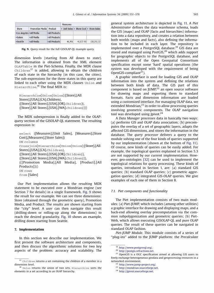
dimension levels (starting from All down to state).The information is obtained from the XML elementOLAPTable in the Piet-Schema. Finally, the MDX clauseChildren17 is added, allowing to obtain the childrenof each state in the hierarchy (in this case, the cities).The sub-expressions for the three states in this query arelinked to each other using the MDX clauses Union andHierarchize.18 The final MDX is:

dim

elem

Hierarchize(Union(Union(f[Store].[AllStores].[USA].[CA].Childreng,f[Store].[All Stores].[USA].[OR].Children)g;f[Store].[All Stores].[USA].[WA].Childreng)))

19 http://www.postgresql.org/.20 http://postgis.refractions.net.

The MDX subexpression is finally added to the OLAP-query section of the GISOLAP-QL statement. The resultingexpression is:

select f[Measures].[Unit Sales], [Measures].[StoreCost],[Measures].[Store Sales]gON columns

Crossjoin(Hierarchize(Union(Union(f[Store].[AllStores].[USA].[CA].Childreng,f[Store].[All Stores].[USA].[OR].Childreng),f[Store].[All Stores].[USA].[WA].Childreng)),f([Promotion Media].[All Media], [Product].[AllProducts])g)ON rows

from [Sales]

Our Piet implementation allows the resulting MDXstatement to be executed over a Mondrian engine (seeSection 7 for details) in a single framework. Fig. 9 showsthe result for our example. We can see three dimensions:Store (obtained through the geometric query), PromotionMedia, and Product. The results are shown starting fromthe ‘‘city’’ level. A user can then navigate this result(drilling-down or rolling-up along the dimensions) toreach the desired granularity. Fig. 10 shows an example,drilling down starting from Seattle.

7. Implementation

In this section we describe our implementation. Wefirst present the software architecture and components,and then discuss the algorithmic solutions for two keyaspects of the problem: accuracy and scalability. The

17 Children returns a set containing the children of a member in a

ension level.18 Union returns the union of two sets, Hierarchize sorts the

ents in a set according to an OLAP hierarchy.

general system architecture is depicted in Fig. 11. A Piet

Administrator defines the data warehouse schema, loadsthe GIS (maps) and OLAP (facts and hierarchies) informa-tion into a data repository, and creates a relation betweenboth worlds (maps and facts), also defining the informa-tion to be included in each layer. The repository isimplemented over a PostgreSQL database.19 GIS data arestored and managed using PostGIS,20 which adds supportfor geographic objects to the PostgreSQL database, andimplements all of the Open Geospatial Consortiumspecification except some ‘hard’ spatial operations (thesystem was developed with the requirement of beingOpenGIS-compliant21).

A graphic interface is used for loading GIS and OLAPinformation into the system and defining the relationsbetween both kinds of data. The GIS part of thiscomponent is based on JUMP,22 an open source softwarefor drawing maps and exporting them to standardformats. Facts and dimension information are loadedusing a customized interface. For managing OLAP data, weextended Mondrian,23 in order to allow processing queriesinvolving geometric components. The OLAP navigationtool was developed using Jpivot.24

A Data Manager processes data in basically two ways:(a) performs GIS and OLAP data association; (b) precom-putes the overlay of a set of geographic layers, adapts theaffected GIS dimensions, and stores the information in thedatabase. The query processor delivers a query to themodule solving one of the four kinds of queries supportedby our implementation (shown at the bottom of Fig. 11).Of course, new kinds of queries can be easily added. Forexample, the topological queries explained in Section 5.3are not supported by our current implementation. How-ever, geo-ontologies [32] can be used to implement thetopological relations for query processing. These kinds ofqueries, introduced in Section 1, are: (a) standard GISqueries; (b) standard OLAP queries; (c) geometric aggre-gation queries; (d) integrated GIS-OLAP queries. We giveexamples of each one of them in Section 8.

7.1. Piet components and functionality

The Piet implementation consists of two main mod-ules: (a) Piet-JUMP, which includes (among other utilities)a graphic interface for drawing and displaying maps, and aback-end allowing overlay precomputation via the com-mon subpolygonization and geometric queries; (b) Piet-Web, which allows executing GISOLAP-QL and pure OLAPqueries. The result of these queries can be navigated instandard OLAP fashion.

Piet-JUMP Module. This module consists of a series of‘‘plug-ins’’ added to the JUMP platform: the Precalculate

21 OpenGIS is a OGC specification aimed at allowing GIS users to

freely exchange heterogeneous geodata and geoprocessing resources in a

networked environment.22 http://www.jump-project.org/.23 http://mondrian.sourceforge.net.24 http://jpivot.sourceforge.net.

http://www.postgresql.org/

http://postgis.refractions.net

http://www.jump-project.org/

http://mondrian.sourceforge.net

http://jpivot.sourceforge.net

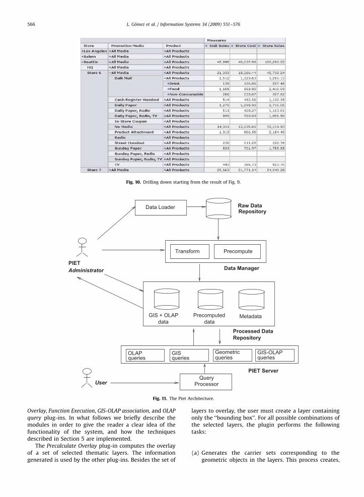
ARTICLE IN PRESS

Fig. 10. Drilling down starting from the result of Fig. 9.

Geometric

User

datadataMetadataPrecomputedGIS + OLAP

Data Loader

queriesqueries queriesGISOLAP

queriesGIS-OLAP

PIETAdministrator

PIET Server

RepositoryProcessed Data

Data Manager

Raw DataRepository

Transform

ProcessorQuery

Precompute

Fig. 11. The Piet Architecture.


Overlay, Function Execution, GIS-OLAP association, and OLAP

query plug-ins. In what follows we briefly describe themodules in order to give the reader a clear idea of thefunctionality of the system, and how the techniquesdescribed in Section 5 are implemented.

The Precalculate Overlay plug-in computes the overlayof a set of selected thematic layers. The informationgenerated is used by the other plug-ins. Besides the set of

layers to overlay, the user must create a layer containingonly the ‘‘bounding box’’. For all possible combinations ofthe selected layers, the plugin performs the followingtasks:

(a)
Generates the carrier sets corresponding to thegeometric objects in the layers. This process creates,

ARTICLE IN PRESS

2

supp


for each possible combination, a table containing thegenerated carrier lines.

(b)
Computes the common subpolygonization of the layer
combination. In this step, the new geometry levels inthe schema are obtained, namely: nodes, open poly-lines, and open polygons. This information is stored ina different table for each geometry, and each element isassigned a unique identifier.

(c)
Associates the original geometric objects to the newlygenerated ones. This is the most computationallyexpensive process. The JTS Topology Suite25 wasextended and improved (see below) for this task.The information obtained is stored in the database (inone table for each level, for each layer combination) inthe form hid of an element of the subpolygonization, id of
the original geometric elementi pairs.
(d) Propagates the values of the density functions to the
objects in the subpolygonization. This is performed inparallel with the association process explained above.

Finally, for each combination of layers, we find all theelements in the subpolygonization that are common tomore than one original geometric object. In the database,a table is generated for each layer combination, and foreach geometry in the subpolygonization (i.e., node, openline, open polygon). A tuple in each table contains theunique identifier of a geometric object, and the uniqueidentifier of the object in the subpolygonization.

The Function Execution plug-in computes a densityfunction defined in a thematic layer, within a query region

(or the entire bounding box if the query region is notdefined). The result is a new layer with the geometricobjects in the subpolygonization and their correspondingfunction values. Along with the selected query region, adensity function is also defined. Two kinds of subpolygo-nizations can be used: full subpolygonization (when all

the layers are overlayed) or partial subpolygonization(when the overlay involves only a subset of the layers). Inthe second case the process is faster, but precision may beunacceptable, depending on how well the polygons fit thequery region.

The GIS-OLAP association plug-in associates spatialinformation to information in a data warehouse. Thisinformation is used by the ‘‘OLAP query’’ plugin and thePiet-Web module. A table contains the unique identifier ofthe geometric object, the unique identifier of the corre-sponding object in the data warehouse, and, optionally, adescription of such object.

The OLAP query plug-in joins the two modules thatcompose the implementation. For a given spatial queryand an OLAP model, the plugin generates and executes anMDX query that merges both kinds of data, and is thenpassed on to an OLAP tool.

Piet-Web Module. This module handles GISOLAP-QLqueries, spatial aggregation queries, and even pure OLAPqueries. In all cases, the result is a dataset that can benavigated using any OLAP tool. This module includes: (a)

5 JTS is an API providing fundamental geometric functions,

orting the OCG model. See http://www.vividsolutions.com/jcs/.

the GISOLAP-QL parser; (b) a translator to SQL; (c) amodule for merging spatial and MDX queries throughquery re-writing, as explained in Section 6.

7.2. Robustness and scalability issues

As with all numerical computation using finite-preci-sion numbers, geometric algorithms included in Piet maypresent problems of robustness, i.e., incorrect results dueto round-off errors. Many basic operations in the JTSlibrary used in the Piet implementation have not yet beenoptimized and tuned. Thus, we extended and improvedthis library, resulting in the so-called Piet-Utils library.Additionally, the subpolygonization of the overlayedlayers generates a huge number of geometric elements.In this setting, scalability issues must be addressed, toguarantee performance in practical real-world situations.Thus, we propose a partition of the map using a grid,which optimizes the computation of the subpolygoniza-tion while preserving its geometric properties.

7.2.1. Robustness

We address separately the computation of the carrierlines and the subpolygonization process.

Computation of carrier lines. In a Piet environment,geometric elements are internally represented using thevector model. The JTS library is composed of objects oftype geometry. Some examples of instances of theseobjects are: POINT (378 145), LINESTRING (191 300, 280319, 350 272, 367 300), and POLYGON (83 215, 298 213,204 74, 120 113, 83 215). Each geometric componentincludes the name and a list of vertices, as pairs of ðX;YÞcoordinates.

The first step of the subpolygonization process is thegeneration of a list containing the carrier lines producedby the carrier sets of the geometric components of eachlayer. The original JTS functions may produce duplicatedcarrier lines, arising from the incorrect overlay of(apparently) similar geometric objects. For instance, if ariver in one layer coincides with a state boundary inanother layer, duplicated carrier lines may appear due tomathematical errors, and propagate to the polygonizationstep. The algorithm used in Piet eliminates these dupli-cated carrier lines after the carrier set is generated.

We also address the problem of minimizing themathematical errors that may appear in the computationof the intersection between carrier lines in differentlayers. First, given a set of carrier lines L1; L2; . . . ; Ln; theintersection between them is computed one line at a time,picking a line Li; i ¼ 1;n� 1; and computing its intersec-tion with Liþj; jX1: Thus, the intersection between twolines Lk; Ls is always computed only once. However, it isstill possible that three or more lines intersect in pointsvery close to each other. In this case, we use a booleanfunction called isSimilarPoint, which, given twopoints and an error bound (set by the user), decides ifthe points are or are not the same (if the points aredifferent they will generate new polygons). There is also afunction addCutPoint which receives a point p and a listP of points associated to a carrier line L: This function is

http://www.vividsolutions.com/jcs/

ARTICLE IN PRESS


used while computing the intersection of L with the rest ofthe carrier lines. If there is a point in P, ‘‘similar’’ to p; thenp is not added to P (i.e., no new cut point is generated).The points are stored sorted according to their distance tothe origin, in order to speed-up the similarity search.

As an example, consider three carrier lines: L1; L2 andL3: P1 is the point where L1 intersects L2 and L3. Alsoassume that the algorithm that generates the sub-nodes iscurrently usingL2 as pivot line (i.e., L1 was already used,and L3 is still waiting). The algorithm computes theintersection between L2 and L3; which happens to be apoint P3 very close to P1: If the difference is less than agiven threshold, P3 will not be added to the list ofcutpoints for L2: The same will happen for L3:

Subpolygonization: The points where the carrier setsintersect each other generate objects denoted sub-lines.From these sub-lines, sub-polygons are computed. Thisinformation is stored in the postGIS database. The sub-polygons are produced using a JTS class called Polygonizer.Our improvements to the JTS library ensure that noduplicated sub-lines will be used to generate the sub-polygons. Further, the sub-lines that the Polygonizerreceives do not include the lines generated by thebounding box.

The most costly process is the association of the sub-geometries to the original geometries. For this computa-tion we also devised some techniques to improve thefunctions provided by the JTS library. For instance, due tomathematical errors, two adjacent sub-polygons mayappear as overlapping geometries. As a consequence, theJTS intersection function provided by JTS would, erro-neously, return True. We replaced this function with a newone, a boolean function denoted OverlapPg (again,‘‘error’’ is defined by the user), which receives twoobjects and a given error threshold, and returns True iftheir overlapping area is larger than such threshold.

7.2.2. Scalability

The subpolygonization process is a huge CPU andmemory consumer. Even though Property 1 shows thatthe planar subdivision is quadratic in the worst case, forlarge maps, the number of sub-geometry elementsproduced may be unacceptable for some hardwarearchitectures. This becomes worse for a high number oflayers involved in the subpolygonization. In order toaddress this issue, we do not compute the commonsubpolygonization over an entire map. Instead, we furtherdivide the map into a grid, and compute separately thesubpolygonization within each rectangle in the grid. Thisscheme produces sub-polygons only where they areneeded. For instance, in our running example, we have alayer with volcanoes in the northern hemisphere. Thedensity of the volcanoes is higher in the western region,and decreases toward the east. Therefore, a huge portionof the map, without any object of interest, would beaffected by the carrier lines generated by the subpolygo-nization. Besides, a carrier line generated by a volcano inthe west would impact a region in the east. It would bemore natural that the influence of a carrier line remainswithin the ‘‘neighborhood’’ of the geometric object thatgenerates it. The grid subdivision solves these problems.

Reducing the number of geometric objects generated bythe subpolygonization, of course, also reduces the size ofthe final database. Also note that the squares in the gridcould be of different sizes. In addition, it would bepossible to compute the polygonization of the squares inthe grid in parallel, provided the necessary hardware isavailable. As a remark, note that the grid partition alsoallows the refinement of a particular rectangle, if, forinstance, this rectangle is overloaded with geometricobjects. Finally, note that geographies can be updated.For instance, a city may grow, a country may be split oreven integrated with another one. Since these changes, ingeneral, only affect a portion of a map, only the commonsubpolygonization for the affected rectangles must berecomputed, and the rest of the map would remainunchanged.

Implementing and using the grid. The grid partition isimplemented as a relational table, denoted gis_quadrant,containing the geometry and identifier of each rectangle(i.e., the table contains as many tuples as rectangles are inthe grid). In addition, a table is generated for each layer,containing only the non-empty grid partitions. In ourrunning example, we have a table volcanoes_grid, whereonly the squares containing a volcano are stored (about10% of the total grid). This dramatically reduces thesubpolygonization time (which uses these tables, insteadof the original ones), as we report in Section 8. The gridpartitioning improves, in many cases, query processing.Since the map overlays are precomputed, query evaluationreduces to compute aggregations over the tables containing

these overlays. When attribute information is needed, ajoin with the tables storing the result of the subpolygo-nization process is also needed. Due to grid partitioning,these tables only contain the subpolygons of interest,

speeding up query execution time. When a query mustbe executed constrained to a query region defined atrunning time (Fig. 12), the intersection between the gridand the query region must becomputed on-the-fly, whichimpacts in the query execution times, as we show inSection 8. Nevertheless, the grid partitioning allows thatto just compute the intersection for the affected rectan-gles, obtaining an important improvement in the perfor-mance of these queries.

The size of the grid is defined in a trial-and-erroriterative process. This process starts with a size that ischosen according to the kinds of maps at hand, until weobtain a grid that results in an acceptable subpolygoniza-tion time (of course, the available hardware plays animportant role here). As an example, in our experiments ofSection 8, we used a grid has one thousand squares(20� 50), having started from a grid of four squares(2� 2).

8. Experimental evaluation

We discuss the results of a set of tests, aimed atproviding evidence that the overlay precomputationmethod, for a wide class of geometric queries (with orwithout aggregation), outperforms other well-establishedmethods like R-tree [14] and aggregation R-tree (aR-tree)

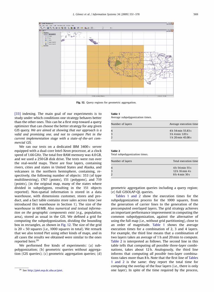
ARTICLE IN PRESS

Fig. 12. Query regions for geometric aggregation.

Table 1Average subpolygonization times.

Number of layers Average execution time

4 4 h 54 min 55.83 s

3 3 h 4 min 1.03 s

2 1 h 20 min 45.08 s

Table 2Total subpolygonization times.

Number of layers Total execution time

4 4 h 54 min 55 s

3 12 h 16 min 4 s

2 8 h 4 min 30 s


[33] indexing. The main goal of our experiments is tostudy under which conditions one strategy behaves betterthan the other ones. This can be a first step toward a queryoptimizer that can choose the better strategy for any givenGIS query. We are aimed at showing that our approach is a

valid and promising one, and not to compare Piet in the

current implementation stage with a state-of-the-art com-

mercial GIS.

We ran our tests on a dedicated IBM 3400� serverequipped with a dual-core Intel-Xeon processor, at a clockspeed of 1.66 GHz. The total free RAM memory was 4.0 GB,and we used a 250 GB disk drive. The tests were run overthe real-world maps. There are four layers, containingrivers, cities and states in United States and Alaska, andvolcanoes in the northern hemisphere, containing, re-spectively, the following number of objects: 353 (of typemultilinestring), 1767 (points), 151 (polygons), and 719(points), (in the original map, many of the states wheredivided in subpolygons, resulting in the 151 objectsreported). Non-spatial information is stored in a datawarehouse, with dimensions customer, stores and pro-duct, and a fact table contains store sales across time (weintroduced this warehouse in Section 1). The size of thewarehouse in 60 MB. Also numerical and textual informa-

tion on the geographic components exist (e.g., population,area), stored as usual in the GIS. We defined a grid forcomputing the subpolygonization, dividing the boundingbox in rectangles, as shown in Fig. 12. The size of the gridis 20� 50 squares (i.e., 1000 squares in total). We remarkthat we also tested Piet using other kinds of maps, and inall cases the results we obtained were similar to the onesreported here.26

We performed five kinds of experiments: (a) sub-polygonization; (b) geometric queries without aggrega-tion (GIS queries); (c) geometric aggregation queries; (d)

26 See http://piet.exp.dc.uba.ar/piet.

geometric aggregation queries including a query region;(e) full GISOLAP-QL queries.

Tables 1 and 2 show the execution times for thesubpolygonization process for the 1000 squares, fromthe generation of carrier lines to the generation of theprecomputed overlayed layers. The grid strategy achievesan important performance improvement in computing thecommon subpolygonization, against the alternative ofusing the full map (i.e., without grid partitioning), close toan order of magnitude. Table 1 shows the averageexecution times for a combination of 2, 3 and 4 layers.For example, the third line means that a combination oftwo layers takes an average of 1 h and 20 min to compute.Table 2 is interpreted as follows. The second line in thistable tells that computing all possible three-layer combi-nations, takes about 12 h. Analogously, the third lineinforms that computing all possible two-layer combina-tions takes more than 8 h. Note that the first line of Tables1 and 2 is the same: they report the total time forcomputing the overlay of the four layers (i.e., there is onlyone layer). In spite of the time required by the process,

http://piet.exp.dc.uba.ar/piet

ARTICLE IN PRESS


note that precomputing the subpolygonization is per-formed off-line, in the same way view materialization iscomputed usually in OLAP. Also, since we use the gridpartitioning strategy, updates are likely to be performedwithin a reasonable time window (see discussion inSection 7). Table 3 reports the maximum, minimum, andaverage number of elements in the sub-geometries in thegrid rectangles, for the combination of the four layers. Wealso compared the sizes of the database before and aftercomputing the subpolygonization: the initial size of thedatabase is 166 MB. After the precomputation of theoverlay of the four layers, the database occupies 621 MB.Although this seems to be an important increase indatabases size, all possible layer overlay combinationswere materialized, with no compression of any kind (i.e.,the worst case). If needed, a partial materializationstrategy (along the lines of [19]) can be applied. Notethat even though the size of the database is moderate, webelieve that the maximum number of sub-geometries perrectangle is high enough for making the experiments

Table 3Number of sub-geometries in the grid for the 4-layers overlay.

Sub-geometry Max. Min. Avg.

# of carrier lines per rectangle 616 4 15

# of points per rectangle

(carrier lines intersection in a rectangle) 107 880 4 452

# of segment lines per rectangle

(segments of carrier lines in a rectangle) 212 256 4 868

# of polygons per rectangle 104 210 1 396

Table 4Geometric queries.

Query Method Code

Q1: List the states that

contain at least one volcano

PostGIS without spatial

indexing

SELECT DIS

volcano.ge

PostGIS with spatial

indexing

SELECT DIS

&& volcano

Piet SELECT DIS

Q2: List the states and the

cities within them


indexing

SELECT sta

city.geome


indexing

SELECT sta

city.geome

Piet SELECT p1.

Q3: List states and the cities

within them, only for states

crossed by at least one river


indexing

SELECT DIS

contains(st

river WHE


indexing

SELECT DIS

&& city.geo

(SELECT st

AND inters

Piet SELECT DIS

(SELECT p2

Q4: List states crossed by al

least ten rivers


indexing

SELECT p1.

p2.geomet


indexing

SELECT p1.

AND inters

count(p2.p

Piet SELECT p1.

count(disti

significant, also considering that we work with real-worldmaps.

For tests of type (b), we selected four geometric queriesthat compute the intersection between different combi-nations of layers, without aggregation. The queries wereevaluated over the entire map (i.e., no query region wasspecified). Table 4 shows the queries and their expressionsin the three query languages. Note that we have chosen toshow, in Tables 4 and 5, the SQL translations of the Pietqueries. In this way, the tables containing the overlayprecomputation (with prefix gis_pre_), and the subpoly-gonization tables (with prefix gis_subp_) are displayed.We first ran the queries generated by Piet against thePostgreSQL database. We then ran equivalent queries withPostGIS, which uses an R-tree implemented using GiST—

Generalized index search tree—[20]. Finally, we ran thepostGIS queries without indexing for the postGIS queries.

Remark 2. Although we cannot claim that PostGIS is thebest implementation of R-trees, we believe that it isappropriate to compare it against our implementation. Itis a well-established and recognized product, and profes-sional developers have participated in its implementation.On the contrary, Piet is still at a proof-of-concept stage.Thus, we believe this is a fair comparison.

The following are the conditions under which the testswere run: (a) all the layers were indexed (see Fig. 17 forindex sizes); (b) all PostGIS queries have been optimizedanalyzing the generated query plans in order to obtain thebest possible performance; (c) all Piet tables have beenindexed over attributes that participate in a join or in a

TINCT state.piet_id FROM state, volcano WHERE contains(state.geometry,

ometry)

TINCT state.piet_id FROM state, volcano WHERE state.geometry

.geometry AND contains(state.geometry, volcano.geometry)

TINCT p1.state FROM gis_pre_point_9 p1

te.id, city.id FROM state, city WHERE contains(state.geometry,

try)

te.piet_id, city.piet_id FROM state, city WHERE state.geometry &&

try AND contains(state.geometry, city.geometry)

state, p1.city FROM gis_pre_point_11 p1

TINCT state.piet_id , city.piet_id FROM state, city WHERE

ate.geometry, city.geometry) AND state.id in (SELECT state.id FROM state,

RE intersects(state.geometry, river.geometry))

TINCT state.piet_id , city.piet_id FROM state, city WHERE state.geometry

metry AND contains(state.geometry, city.geometry) AND state.piet_id in

ate.piet_id FROM state, river WHERE state.geometry && river.geometry

ects(state.geometry, river.geometry))

TINCT p1.state, p1.city FROM gis_pre_point_11 p1 WHERE p1.state IN

.state FROM gis_pre_linestring_7 p2)

piet_id FROM state p1, river p2 WHERE intersects(p1.geometry,

ry) GROUP BY p1.piet_id HAVING count(p2.piet_id) 4 ¼ 10

piet_id FROM state p1, river p2 WHERE p1.geometry && p2.geometry

ects(p1.geometry, p2.geometry) GROUP BY p1.piet_id HAVING

iet_id) 4 ¼ 10

state FROM gis_pre_linestring_7 p1 GROUP BY p1.state HAVING

nct p1.river) 4 ¼ 10

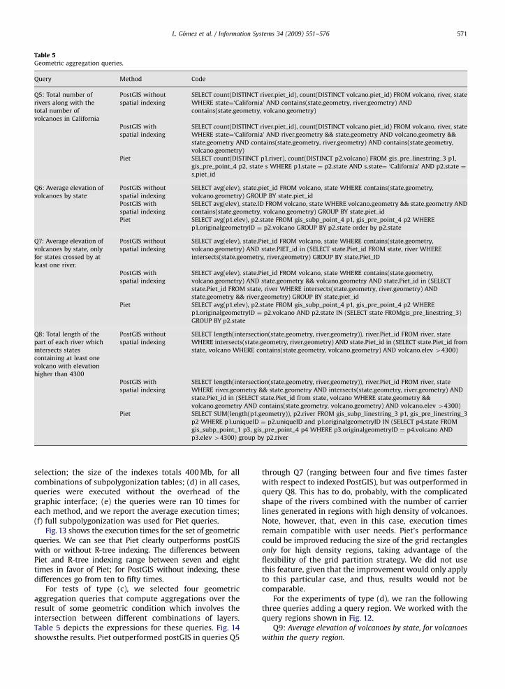
ARTICLE IN PRESS

Table 5Geometric aggregation queries.

Query Method Code

Q5: Total number of

rivers along with the

total number of

volcanoes in California

PostGIS without

spatial indexing

SELECT count(DISTINCT river.piet_id), count(DISTINCT volcano.piet_id) FROM volcano, river, state

WHERE state¼‘California’ AND contains(state.geometry, river.geometry) AND

contains(state.geometry, volcano.geometry)

PostGIS with

spatial indexing

SELECT count(DISTINCT river.piet_id), count(DISTINCT volcano.piet_id) FROM volcano, river, state

WHERE state¼‘California’ AND river.geometry && state.geometry AND volcano.geometry &&

state.geometry AND contains(state.geometry, river.geometry) AND contains(state.geometry,

volcano.geometry)

Piet SELECT count(DISTINCT p1.river), count(DISTINCT p2.volcano) FROM gis_pre_linestring_3 p1,

gis_pre_point_4 p2, state s WHERE p1.state ¼ p2.state AND s.state¼ ‘California’ AND p2.state ¼

s.piet_id

Q6: Average elevation of

volcanoes by state

PostGIS without

spatial indexing

SELECT avg(elev), state.piet_id FROM volcano, state WHERE contains(state.geometry,

volcano.geometry) GROUP BY state.piet_id

PostGIS with

spatial indexing

SELECT avg(elev), state.ID FROM volcano, state WHERE volcano.geometry && state.geometry AND

contains(state.geometry, volcano.geometry) GROUP BY state.piet_id

Piet SELECT avg(p1.elev), p2.state FROM gis_subp_point_4 p1, gis_pre_point_4 p2 WHERE

p1.originalgeometryID ¼ p2.volcano GROUP BY p2.state order by p2.state

Q7: Average elevation of

volcanoes by state, only

for states crossed by at

least one river.

PostGIS without

spatial indexing

SELECT avg(elev), state.Piet_id FROM volcano, state WHERE contains(state.geometry,

volcano.geometry) AND state.PIET_id in (SELECT state.Piet_id FROM state, river WHERE

intersects(state.geometry, river.geometry) GROUP BY state.Piet_ID

PostGIS with

spatial indexing

SELECT avg(elev), state.Piet_id FROM volcano, state WHERE contains(state.geometry,

volcano.geometry) AND state.geometry && volcano.geometry AND state.Piet_id in (SELECT

state.Piet_id FROM state, river WHERE intersects(state.geometry, river.geometry) AND

state.geometry && river.geometry) GROUP BY state.piet_id

Piet SELECT avg(p1.elev), p2.state FROM gis_subp_point_4 p1, gis_pre_point_4 p2 WHERE

p1.originalgeometryID ¼ p2.volcano AND p2.state IN (SELECT state FROMgis_pre_linestring_3)

GROUP BY p2.state

Q8: Total length of the

part of each river which

intersects states

containing at least one

volcano with elevation

higher than 4300

PostGIS without

spatial indexing

SELECT length(intersection(state.geometry, river.geometry)), river.Piet_id FROM river, state

WHERE intersects(state.geometry, river.geometry) AND state.Piet_id in (SELECT state.Piet_id from

state, volcano WHERE contains(state.geometry, volcano.geometry) AND volcano.elev 44300)

PostGIS with

spatial indexing

SELECT length(intersection(state.geometry, river.geometry)), river.Piet_id FROM river, state

WHERE river.geometry && state.geometry AND intersects(state.geometry, river.geometry) AND

state.Piet_id in (SELECT state.Piet_id from state, volcano WHERE state.geometry &&

volcano.geometry AND contains(state.geometry, volcano.geometry) AND volcano.elev 44300)

Piet SELECT SUM(length(p1.geometry)), p2.river FROM gis_subp_linestring_3 p1, gis_pre_linestring_3

p2 WHERE p1.uniqueID ¼ p2.uniqueID and p1.originalgeometryID IN (SELECT p4.state FROM

gis_subp_point_1 p3, gis_pre_point_4 p4 WHERE p3.originalgeometryID ¼ p4.volcano AND

p3.elev 44300) group by p2.river


selection; the size of the indexes totals 400 Mb, for allcombinations of subpolygonization tables; (d) in all cases,queries were executed without the overhead of thegraphic interface; (e) the queries were ran 10 times foreach method, and we report the average execution times;(f) full subpolygonization was used for Piet queries.

Fig. 13 shows the execution times for the set of geometricqueries. We can see that Piet clearly outperforms postGISwith or without R-tree indexing. The differences betweenPiet and R-tree indexing range between seven and eighttimes in favor of Piet; for PostGIS without indexing, thesedifferences go from ten to fifty times.

For tests of type (c), we selected four geometricaggregation queries that compute aggregations over theresult of some geometric condition which involves theintersection between different combinations of layers.Table 5 depicts the expressions for these queries. Fig. 14showsthe results. Piet outperformed postGIS in queries Q5

through Q7 (ranging between four and five times fasterwith respect to indexed PostGIS), but was outperformed inquery Q8. This has to do, probably, with the complicatedshape of the rivers combined with the number of carrierlines generated in regions with high density of volcanoes.Note, however, that, even in this case, execution timesremain compatible with user needs. Piet’s performancecould be improved reducing the size of the grid rectanglesonly for high density regions, taking advantage of theflexibility of the grid partition strategy. We did not usethis feature, given that the improvement would only applyto this particular case, and thus, results would not becomparable.

For the experiments of type (d), we ran the followingthree queries adding a query region. We worked with thequery regions shown in Fig. 12.

Q9: Average elevation of volcanoes by state, for volcanoes

within the query region.

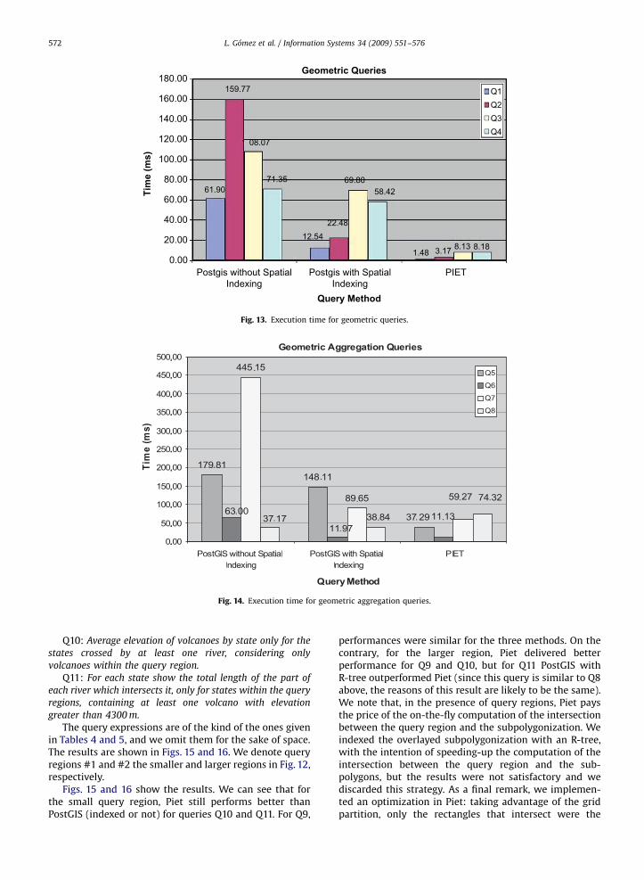
ARTICLE IN PRESS

180.00

160.00

140.00

120.00

100.00

80.00

60.00

40.00

20.00

0.00Postgis without Spatial

IndexingPostgis with Spatial

IndexingPIET

Query Method

Tim

e (m

s)

159.77

08.07

71.3561.90

69.8058.42

22.4812.54

1.48 3.17 8.13 8.18

Q1Q2Q3Q4

Geometric Queries

Fig. 13. Execution time for geometric queries.

Fig. 14. Execution time for geometric aggregation queries.


Q10: Average elevation of volcanoes by state only for the

states crossed by at least one river, considering only

volcanoes within the query region.

Q11: For each state show the total length of the part of

each river which intersects it, only for states within the query

regions, containing at least one volcano with elevation

greater than 4300 m.

The query expressions are of the kind of the ones givenin Tables 4 and 5, and we omit them for the sake of space.The results are shown in Figs. 15 and 16. We denote queryregions #1 and #2 the smaller and larger regions in Fig. 12,respectively.

Figs. 15 and 16 show the results. We can see that forthe small query region, Piet still performs better thanPostGIS (indexed or not) for queries Q10 and Q11. For Q9,

performances were similar for the three methods. On thecontrary, for the larger region, Piet delivered betterperformance for Q9 and Q10, but for Q11 PostGIS withR-tree outperformed Piet (since this query is similar to Q8above, the reasons of this result are likely to be the same).We note that, in the presence of query regions, Piet paysthe price of the on-the-fly computation of the intersectionbetween the query region and the subpolygonization. Weindexed the overlayed subpolygonization with an R-tree,with the intention of speeding-up the computation of theintersection between the query region and the sub-polygons, but the results were not satisfactory and wediscarded this strategy. As a final remark, we implemen-ted an optimization in Piet: taking advantage of the gridpartition, only the rectangles that intersect were the

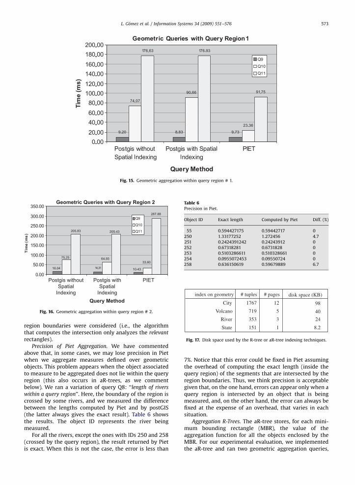
ARTICLE IN PRESS

Fig. 15. Geometric aggregation within query region # 1.

Fig. 16. Geometric aggregation within query region # 2.

Table 6Precision in Piet.

Object ID Exact length Computed by Piet Diff. (%)

55 0.594427175 0.59442717 0

250 1.33177252 1.272456 4.7

251 0.2424391242 0.24243912 0

252 0.67318281 0.6731828 0

253 0.5103286611 0.510328661 0

254 0.0955072453 0.09550724 0

258 0.636150619 0.59679889 6.7

index on geometry # tuples # pages disk space (KB)

City 1767 12 98

Volcano 719 5 40

River 353 3 24

State 151 1 8.2

Fig. 17. Disk space used by the R-tree or aR-tree indexing techniques.


region boundaries were considered (i.e., the algorithmthat computes the intersection only analyzes the relevant

rectangles).Precision of Piet Aggregation. We have commented

above that, in some cases, we may lose precision in Pietwhen we aggregate measures defined over geometricobjects. This problem appears when the object associatedto measure to be aggregated does not lie within the queryregion (this also occurs in aR-trees, as we commentbelow). We ran a variation of query Q8: ‘‘length of rivers

within a query region’’. Here, the boundary of the region iscrossed by some rivers, and we measured the differencebetween the lengths computed by Piet and by postGIS(the latter always gives the exact result). Table 6 showsthe results. The object ID represents the river beingmeasured.

For all the rivers, except the ones with IDs 250 and 258(crossed by the query region), the result returned by Pietis exact. When this is not the case, the error is less than

7%. Notice that this error could be fixed in Piet assumingthe overhead of computing the exact length (inside thequery region) of the segments that are intersected by theregion boundaries. Thus, we think precision is acceptablegiven that, on the one hand, errors can appear only when aquery region is intersected by an object that is beingmeasured, and, on the other hand, the error can always befixed at the expense of an overhead, that varies in eachsituation.

Aggregation R-Trees. The aR-tree stores, for each mini-mum bounding rectangle (MBR), the value of theaggregation function for all the objects enclosed by theMBR. For our experimental evaluation, we implementedthe aR-tree and ran two geometric aggregation queries,

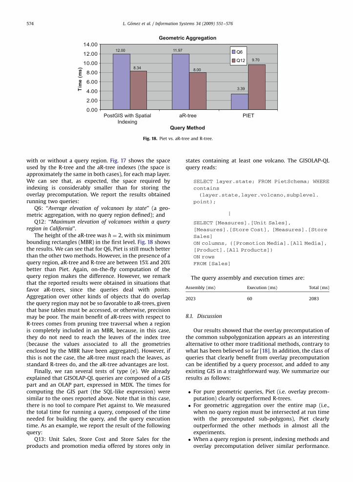
ARTICLE IN PRESS

Fig. 18. Piet vs. aR-tree and R-tree.


with or without a query region. Fig. 17 shows the spaceused by the R-tree and the aR-tree indexes (the space isapproximately the same in both cases), for each map layer.We can see that, as expected, the space required byindexing is considerably smaller than for storing theoverlay precomputation. We report the results obtainedrunning two queries:

Q6: ‘‘Average elevation of volcanoes by state’’ (a geo-metric aggregation, with no query region defined); and

Q12: ‘‘Maximum elevation of volcanoes within a query

region in California’’.The height of the aR-tree was h ¼ 2, with six minimum

bounding rectangles (MBR) in the first level. Fig. 18 showsthe results. We can see that for Q6, Piet is still much betterthan the other two methods. However, in the presence of aquery region, aR-tree and R-tree are between 15% and 20%better than Piet. Again, on-the-fly computation of thequery region makes the difference. However, we remarkthat the reported results were obtained in situations thatfavor aR-trees, since the queries deal with points.Aggregation over other kinds of objects that do overlapthe query region may not be so favorable to aR-trees, giventhat base tables must be accessed, or otherwise, precisionmay be poor. The main benefit of aR-trees with respect toR-trees comes from pruning tree traversal when a regionis completely included in an MBR, because, in this case,they do not need to reach the leaves of the index tree(because the values associated to all the geometriesenclosed by the MBR have been aggregated). However, ifthis is not the case, the aR-tree must reach the leaves, asstandard R-trees do, and the aR-tree advantages are lost.

Finally, we ran several tests of type (e). We alreadyexplained that GISOLAP-QL queries are composed of a GISpart and an OLAP part, expressed in MDX. The times forcomputing the GIS part (the SQL-like expression) weresimilar to the ones reported above. Note that in this case,there is no tool to compare Piet against to. We measuredthe total time for running a query, composed of the timeneeded for building the query, and the query executiontime. As an example, we report the result of the followingquery:

Q13: Unit Sales, Store Cost and Store Sales for theproducts and promotion media offered by stores only in

states containing at least one volcano. The GISOLAP-QLquery reads:

SELECT layer.state; FROM PietSchema; WHERE

contains

(layer.state,layer.volcano,subplevel.

point);

j

SELECT [Measures].[Unit Sales],

[Measures].[Store Cost], [Measures].[Store

Sales]

ON columns, ([Promotion Media].[All Media],

[Product].[All Products])

ON rows

FROM [Sales]

The query assembly and execution times are:

Assembly (ms)
Execution (ms) Total (ms)
2023
60 2083
8.1. Discussion

Our results showed that the overlay precomputation ofthe common subpolygonization appears as an interestingalternative to other more traditional methods, contrary towhat has been believed so far [18]. In addition, the class ofqueries that clearly benefit from overlay precomputationcan be identified by a query processor, and added to anyexisting GIS in a straightforward way. We summarize ourresults as follows:

�
For pure geometric queries, Piet (i.e. overlay precom-putation) clearly outperformed R-trees. � For geometric aggregation over the entire map (i.e.,
when no query region must be intersected at run timewith the precomputed sub-polygons), Piet clearlyoutperformed the other methods in almost all theexperiments.
� When a query region is present, indexing methods and
overlay precomputation deliver similar performance.

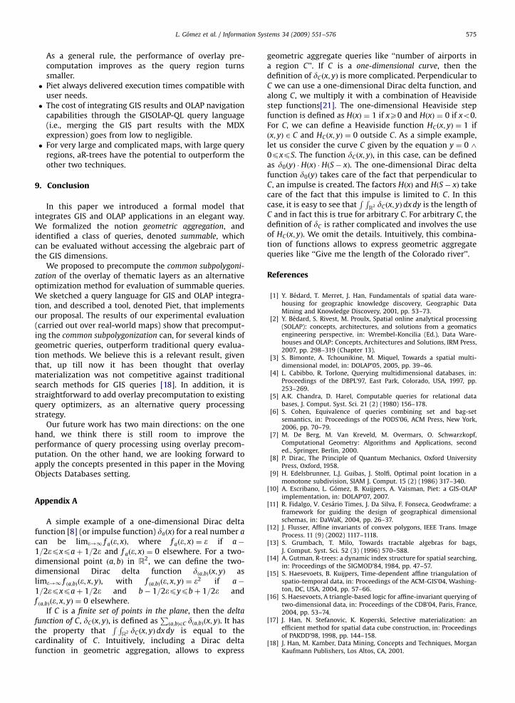
ARTICLE IN PRESS


As a general rule, the performance of overlay pre-computation improves as the query region turnssmaller.
� Piet always delivered execution times compatible with
user needs.
� The cost of integrating GIS results and OLAP navigation
capabilities through the GISOLAP-QL query language(i.e., merging the GIS part results with the MDXexpression) goes from low to negligible.
� For very large and complicated maps, with large query
regions, aR-trees have the potential to outperform theother two techniques.

9. Conclusion

In this paper we introduced a formal model thatintegrates GIS and OLAP applications in an elegant way.We formalized the notion geometric aggregation, andidentified a class of queries, denoted summable, whichcan be evaluated without accessing the algebraic part ofthe GIS dimensions.

We proposed to precompute the common subpolygoni-

zation of the overlay of thematic layers as an alternativeoptimization method for evaluation of summable queries.We sketched a query language for GIS and OLAP integra-tion, and described a tool, denoted Piet, that implementsour proposal. The results of our experimental evaluation(carried out over real-world maps) show that precomput-ing the common subpolygonization can, for several kinds ofgeometric queries, outperform traditional query evalua-tion methods. We believe this is a relevant result, giventhat, up till now it has been thought that overlaymaterialization was not competitive against traditionalsearch methods for GIS queries [18]. In addition, it isstraightforward to add overlay precomputation to existingquery optimizers, as an alternative query processingstrategy.

Our future work has two main directions: on the onehand, we think there is still room to improve theperformance of query processing using overlay precom-putation. On the other hand, we are looking forward toapply the concepts presented in this paper in the MovingObjects Databases setting.

Appendix A

A simple example of a one-dimensional Dirac deltafunction [8] (or impulse function) daðxÞ for a real number a

can be lime!1 f aðe; xÞ; where f aðe; xÞ ¼ e if a�

1=2epxpaþ 1=2e and f aðe; xÞ ¼ 0 elsewhere. For a two-dimensional point ða; bÞ in R2, we can define the two-dimensional Dirac delta function dða;bÞðx; yÞ aslime!1 f ða;bÞðe; x; yÞ, with f ða;bÞðe; x; yÞ ¼ e2 if a�

1=2epxpaþ 1=2e and b� 1=2epypbþ 1=2e andf ða;bÞðe; x; yÞ ¼ 0 elsewhere.

If C is a finite set of points in the plane, then the delta

function of C, dCðx; yÞ, is defined asPða;bÞ2C dða;bÞðx; yÞ. It has

the property thatR R

R2 dCðx; yÞdx dy is equal to thecardinality of C. Intuitively, including a Dirac deltafunction in geometric aggregation, allows to express

geometric aggregate queries like ‘‘number of airports ina region C’’. If C is a one-dimensional curve, then thedefinition of dCðx; yÞ is more complicated. Perpendicular toC we can use a one-dimensional Dirac delta function, andalong C, we multiply it with a combination of Heavisidestep functions[21]. The one-dimensional Heaviside stepfunction is defined as HðxÞ ¼ 1 if xX0 and HðxÞ ¼ 0 if xo0.For C, we can define a Heaviside function HCðx; yÞ ¼ 1 ifðx; yÞ 2 C and HCðx; yÞ ¼ 0 outside C. As a simple example,let us consider the curve C given by the equation y ¼ 0 ^0pxpS. The function dCðx; yÞ, in this case, can be definedas d0ðyÞ � HðxÞ � HðS� xÞ. The one-dimensional Dirac deltafunction d0ðyÞ takes care of the fact that perpendicular toC, an impulse is created. The factors HðxÞ and HðS� xÞ takecare of the fact that this impulse is limited to C. In thiscase, it is easy to see that

R RR2 dCðx; yÞ dx dy is the length of

C and in fact this is true for arbitrary C. For arbitrary C, thedefinition of dC is rather complicated and involves the useof HCðx; yÞ. We omit the details. Intuitively, this combina-tion of functions allows to express geometric aggregatequeries like ‘‘Give me the length of the Colorado river’’.

References

[1] Y. Bedard, T. Merret, J. Han, Fundamentals of spatial data ware-housing for geographic knowledge discovery, Geographic DataMining and Knowledge Discovery, 2001, pp. 53–73.

[2] Y. Bedard, S. Rivest, M. Proulx, Spatial online analytical processing(SOLAP): concepts, architectures, and solutions from a geomaticsengineering perspective, in: Wrembel-Koncilia (Ed.), Data Ware-houses and OLAP: Concepts, Architectures and Solutions, IRM Press,2007, pp. 298–319 (Chapter 13).

[3] S. Bimonte, A. Tchounikine, M. Miquel, Towards a spatial multi-dimensional model, in: DOLAP’05, 2005, pp. 39–46.

[4] L. Cabibbo, R. Torlone, Querying multidimensional databases, in:Proceedings of the DBPL’97, East Park, Colorado, USA, 1997, pp.253–269.

[5] A.K. Chandra, D. Harel, Computable queries for relational databases, J. Comput. Syst. Sci. 21 (2) (1980) 156–178.

[6] S. Cohen, Equivalence of queries combining set and bag-setsemantics, in: Proceedings of the PODS’06, ACM Press, New York,2006, pp. 70–79.

[7] M. De Berg, M. Van Kreveld, M. Overmars, O. Schwarzkopf,Computational Geometry: Algorithms and Applications, seconded., Springer, Berlin, 2000.

[8] P. Dirac, The Principle of Quantum Mechanics, Oxford UniversityPress, Oxford, 1958.

[9] H. Edelsbrunner, L.J. Guibas, J. Stolfi, Optimal point location in amonotone subdivision, SIAM J. Comput. 15 (2) (1986) 317–340.

[10] A. Escribano, L. Gomez, B. Kuijpers, A. Vaisman, Piet: a GIS-OLAPimplementation, in: DOLAP’07, 2007.

[11] R. Fidalgo, V. Cesario Times, J. Da Silva, F. Fonseca, Geodwframe: aframework for guiding the design of geographical dimensionalschemas, in: DaWaK, 2004, pp. 26–37.

[12] J. Flusser, Affine invariants of convex polygons, IEEE Trans. ImageProcess. 11 (9) (2002) 1117–1118.

[13] S. Grumbach, T. Milo, Towards tractable algebras for bags,J. Comput. Syst. Sci. 52 (3) (1996) 570–588.

[14] A. Gutman, R-trees: a dynamic index structure for spatial searching,in: Proceedings of the SIGMOD’84, 1984, pp. 47–57.

[15] S. Haesevoets, B. Kuijpers, Time-dependent affine triangulation ofspatio-temporal data, in: Proceedings of the ACM-GIS’04, Washing-ton, DC, USA, 2004, pp. 57–66.

[16] S. Haesevoets, A triangle-based logic for affine-invariant querying oftwo-dimensional data, in: Proceedings of the CDB’04, Paris, France,2004, pp. 53–74.

[17] J. Han, N. Stefanovic, K. Koperski, Selective materialization: anefficient method for spatial data cube construction, in: Proceedingsof PAKDD’98, 1998, pp. 144–158.

[18] J. Han, M. Kamber, Data Mining, Concepts and Techniques, MorganKaufmann Publishers, Los Altos, CA, 2001.

ARTICLE IN PRESS


[19] V. Harinarayan, A. Rajaraman, J. Ullman, Implementing data cubesefficiently, in: Proceedings of the SIGMOD’96, Montreal, Canada,1996, pp. 205–216.

[20] J. Hellerstein, J. Naughton, A. Pfeffer, Generalized search trees fordatabase systems, in: VLDB, 1995, pp. 562–573.

[21] R. Hoskins, Generalised Functions, Ellis Horwood Series: Mathe-matics and its Applications, Wiley, New York, 1979.

[22] C. Hurtado, A. Mendelzon, A. Vaisman, Maintaining data cubesunder dimension updates, in: Proceedings of the IEEE/ICDE’99,1999, pp. 346–355.

[23] C. Jensen, A. Kligys, T. Pedersen, I. Timko, Multidimensional datamodeling for location-based services, VLDB J. 13 (1) (2004) 1–21.

[24] R. Kimball, The Data Warehouse Toolkit, Wiley, New York, 1996.[25] A. Klug, Equivalence of relational algebra and relational calculus query

languages having aggregate functions, J. ACM 29 (3) (1982) 699–717.[26] B. Kuijpers, D.V. Gucht, Genericity in spatial databases, in: J.

Paredaens, G. Kuper, L. Libkin (Eds.), Constraint Databases, Springer,Berlin, 2000, pp. 293–304 (Chapter 12).

[27] G. Kuper, M. Scholl, Geographic information systems, in: J.Paredaens, G. Kuper, L. Libkin (Eds.), Constraint Databases, Springer,Berlin, 2000, pp. 175–198 (Chapter 12).

[28] H. Lenz, A. Shoshani, Summarizability in OLAP and statistical databases, in: Proceedings of the Ninth International Conference onScientific and Statistical Database Management, August 11–13, 1997,Olympia, Washington, USA, IEEE Computer Society, 1997, pp. 132–143.

[29] E. Malinowski, E. Zimanyi, OLAP hierarchies: a conceptual perspec-tive, in: CAiSE, 2004, pp. 477–491.

[30] E. Malinowski, E. Zimanyi, Representing spatiality in a conceptualmultidimensional model, in: GIS, 2004, pp. 12–22.

[31] E. Malinowski, E. Zimanyi, Logical representation of a conceptualmodel for spatial data warehouses, Geoinformatica 11 (4) (2007)431–457.

[32] O. Nigro, S.G. Cisaro, D. Xodo, Data Mining with Ontologies:Implementations, Findings and Frameworks, Idea Group, 2007.

[33] D. Papadias, P. Kalnis, J. Zhang, Y. Tao, Efficient OLAP operations inspatial data warehouses, in: Proceedings of the SSTD’01, 2001,pp. 443–459.

[34] D. Papadias, Y. Tao, P. Kalnis, J. Zhang, Indexing spatio-temporaldata warehouses, in: Proceedings of the ICDE’02, 2002, pp. 166–175.

[35] C.H. Papadimitriou, D. Suciu, V. Vianu, Topological queries in spatialdatabases, in: Proceedings of the PODS’96, ACM Press, New York,1996, pp. 81–92.

[36] J. Paredaens, J.V. den Bussche, D.V. Gucht, Towards a theory ofspatial database queries, in: Proceedings of the PODS’94, New York,1994, pp. 279–288.

[37] J. Paredaens, G. Kuper, L. Libkin (Eds.), Constraint databases,Springer, Berlin, 2000.

[38] T. Pedersen, N. Tryfona, Pre-aggregation in spatial data warehouses,in: Proceedings of the SSTD’01, 2001, pp. 460–480.

[39] E. Pourabas, Cooperation with geographic databases, in: M.Raffanelli (Ed.), Multidimensional Databases, Idea Group, 2003,pp. 166–199 (Chapter 13).

[40] F. Rao, L. Zang, X. Yu, Y. Li, Y. Chen, Spatial hierarchy and OLAP-favored search in spatial data warehouse, in: Proceedings of theDOLAP’03, Louisiana, USA, 2003, pp. 48–55.

[41] P. Rigaux, M. Scholl, A. Voisard, Spatial Databases, MorganKaufmann, Los Altos, CA, 2002.

[42] S. Rivest, Y. Bedard, P. Marchand, Toward better support forspatial decision making: defining the characteristics of spatial,on-line analytical processing (SOLAP), Geomatica 55 (4) (2001)539–555.

[43] S. Shekhar, C. Lu, X. Tan, S. Chawla, R. Vatsavai, Mapcube: avisualization tool for spatial data warehouses, in: H. Miller, J. Han(Eds.), Geographic Data Mining and Knowledge Discovery (GKD),Taylor & Francis, London, 2001, pp. 74–109.

[44] A. Shoshani, OLAP and statistical databases: similarities anddifferences, in: Proceedings of the ACM TODS, 1997.

[45] N. Stefanovic, J. Han, K. Koperski, Object-based selective materi-alization for efficient implementation of spatial data cubes, IEEETrans. Knowl. Data Eng. 12 (6) (2000) 938–958.

[46] J.d. Silva, A. Cesario Times, V. Salgado, An open source and webbased framework for geographic and multidimensional processing,in: SAC, 2006, pp. 63–67.

[47] J.d. Silva, A.S. Castro Vera, A. Oliveira, R. Fidalgo, A. Salgado, V.Times, Querying geographical data warehouses with GEOMDQL, in:SBBD, 2007, pp. 223–237.

[48] I. Vega Lopez, R. Snodgrass, B. Moon, Spatiotemporal aggregatecomputation: a survey, IEEE Trans. Knowl. Data Eng. 17 (2) (2005)271–286.

[49] M.F. Worboys, GIS: A Computing Perspective, Taylor & Francis,London, 1995.

[50] L. Zang, Y. Li, F. Rao, X. Yu, Y. Chen, An approach to enabling spatialOLAP by aggregating on spatial hierarchy, in: Proceedings of theDaWak’03, Prague, Czech Republic, 2003, pp. 35–44.

Spatial aggregation Data model and implementation · Spatial aggregation: Data model and...

Documents

Transcript of Spatial aggregation Data model and implementation · Spatial aggregation: Data model and...