Sparse Discriminant Analysis

Line Clemmensen∗ Trevor Hastie∗∗ Daniela Witten+ Bjarne Ersbøll∗

∗Department of Informatics and Mathematical Modelling,

Technical University of Denmark, Kgs. Lyngby, Denmark

∗∗Department of Statistics, Stanford University, Stanford CA, U.S.A.

+Department of Biostatistics, University of Washington, Seattle WA, U.S.A.

April 16, 2011

Abstract

We consider the problem of performing interpretable classification in the

high-dimensional setting, in which the number of features is very large and the

number of observations is limited. This setting has been studied extensively

in the chemometrics literature, and more recently has become commonplace

in biological and medical applications. In this setting, a traditional approach

involves performing feature selection before classification. We propose sparse

discriminant analysis, a method for performing linear discriminant analysis

with a sparseness criterion imposed such that classification and feature selec-

tion are performed simultaneously. Sparse discriminant analysis is based on

the optimal scoring interpretation of linear discriminant analysis, and can be

extended to perform sparse discrimination via mixtures of Gaussians if bound-

aries between classes are non-linear or if subgroups are present within each

class. Our proposal also provides low-dimensional views of the discriminative

directions.

1

1 Introduction

Linear discriminant analysis (LDA) is a favored tool for supervised classification in

many applications, due to its simplicity, robustness, and predictive accuracy (Hand,

2006). LDA also provides low-dimensional projections of the data onto the most

discriminative directions, which can be useful for data interpretation. There are

three distinct arguments that result in the LDA classifier: the multivariate Gaussian

model, Fisher’s discriminant problem, and the optimal scoring problem. These are

reviewed in Section 2.1.

Though LDA often performs quite well in simple, low-dimensional settings, it is

known to fail in the following cases:

• When the number of predictor variables p is large relative to the number of

observations n. In this case, LDA cannot be applied directly because the within-

class covariance matrix of the features is singular.

• When a single prototype per class is insufficient.

• When linear boundaries cannot separate the classes.

Moreover, in some cases where p n, one may wish for a classifier that performs

feature selection - that is, a classifier that involves only a subset of the p features.

Such a sparse classifier ensures easier model interpretation and may reduce overfitting

of the training data.

In this paper, we develop a sparse version of LDA using an `1 or lasso penalty

(Tibshirani, 1996). The use of an `1 penalty to achieve sparsity has been studied

extensively in the regression framework (Tibshirani, 1996; Efron et al., 2004; Zou

and Hastie, 2005; Zou et al., 2006). If X is a n× p data matrix and y is an outcome

vector of length n, then the lasso solves the problem

minimizeβ||y −Xβ||2 + λ||β||1 (1)

2

and the elastic net (Zou and Hastie, 2005) solves the problem

minimizeβ||y −Xβ||2 + λ||β||1 + γ||β||2 (2)

where λ and γ are nonnegative tuning parameters. When λ is large, then both

the lasso and the elastic net will yield sparse coefficient vector estimates. Through

the additional use of an `2 penalty, the elastic net provides some advantages over

the lasso: correlated features tend to be assigned similar regression coefficients, and

more than min(n, p) features can be included in the model. In this paper, we apply

an elastic net penalty to the coefficient vectors in the optimal scoring interpretation

of LDA in order to develop a sparse version of discriminant analysis. This is related

to proposals by Grosenick et al. (2008) and Leng (2008). Since our proposal is based

on the optimal scoring framework, we are able to extend it to mixtures of Gaussians

(Hastie and Tibshirani, 1996).

There already exist a number of proposals to extend LDA to the high-dimensional

setting. Some of these proposals involve non-sparse classifiers. For instance, within

the multivariate Gaussian model for LDA, Dudoit et al. (2001) and Bickel and Levina

(2004) assume independence of the features (naive Bayes), and Friedman (1989) sug-

gests applying a ridge penalty to the within-class covariance matrix. Other positive

definite estimates of the within-class covariance matrix are considered by Krzanowski

et al. (1995) and Xu et al. (2009). Some proposals that lead to sparse classifiers have

also been considered: Tibshirani et al. (2002) adapt the naive Bayes classifier by soft-

thresholding the mean vectors, and Guo et al. (2007) combine a ridge-type penalty

on the within-class covariance matrix with a soft-thresholding operation. Witten

and Tibshirani (2011) apply `1 penalties to Fisher’s discriminant problem in order

to obtain sparse discriminant vectors, but this approach cannot be extended to the

Gaussian mixture setting and lacks the simplicity of the regression-based optimal

3

scoring approach that we take in this paper.

The rest of this paper is organized as follows. In Section 2, we review LDA and

we present our proposals for sparse discriminant analysis and sparse mixture discrim-

inant analysis. Section 3 briefly describes three methods to which we will compare

our proposal: shrunken centroids regularized discriminant analysis, sparse partial

least squares, and elastic net regression of dummy variables. Section 4 contains

experimental results, and the discussion is in Section 5.

2 Methodology

2.1 A review of linear discriminant analysis

Let X be a n× p data matrix, and suppose that each of the n observations falls into

one of K classes. Assume that each of the p features has been centered to have mean

zero, and that the features have been standardized to have equal variance if they are

not measured on the same scale. Let xi denote the ith observation, and let Ck denote

the indices of the observations in the kth class. Consider a very simple multivariate

Gaussian model for the data, in which we assume that an observation in class k is

distributed N(µk,Σw) where µk ∈ Rp is the mean vector for class k and Σw is a p×p

pooled within-class covariance matrix common to all K classes. We use 1|Ck|∑

i∈Ckxi

as an estimate for µk, and we use 1n

∑Kk=1

∑i∈Ck

(xi − µk)(xi − µk)T as an estimate

for Σw (see e.g. Hastie et al., 2009). The LDA classification rule then results from

applying Bayes’ rule to estimate the most likely class for a test observation.

LDA can also be seen as arising from Fisher’s discriminant problem. Define the

between-class covariance matrix Σb =∑K

k=1 πkµkµTk , where πk is the prior probabil-

ity for class k (generally estimated as the fraction of observations belonging to class

k). Fisher’s discriminant problem involves seeking discriminant vectors β1, . . . ,βK−1

4

that successively maximize

maximizeβkβT

kΣbβk subject to βTkΣwβk = 1,βT

kΣwβl = 0 ∀l < k. (3)

Since Σb has rank at most K−1, there are at most K−1 non-trivial solutions to the

generalized eigen problem (3), and hence at most K − 1 discriminant vectors. These

solutions are directions upon which the data has maximal between-class variance rel-

ative to its within-class variance. One can show that nearest centroid classification

on the matrix

(Xβ1 · · ·XβK−1

)yields the same LDA classification rule as the mul-

tivariate Gaussian model described previously (see e.g. Hastie et al., 2009). Fisher’s

discriminant problem has an advantage over the multivariate Gaussian interpretation

of LDA, in that one can perform reduced-rank classification by performing nearest

centroid classification on the matrix

(Xβ1 · · ·Xβq

)with q < K − 1. One can show

that performing nearest centroid classification on this n× q matrix is exactly equiv-

alent to performing full-rank LDA on this n × q matrix. We will make use of this

fact later. Fisher’s discriminant problem also leads to a tool for data visualization,

since it can be informative to plot the vectors Xβ1, Xβ2, and so on.

In this paper, we will make use of optimal scoring, a third formulation that yields

the LDA classification rule and is discussed in detail in Hastie et al. (1995). It involves

recasting the classification problem as a regression problem by turning categorical

variables into quantitative variables, via a sequence of scorings. Let Y denote a

n×K matrix of dummy variables for the K classes; Yik is an indicator variable for

whether the ith observation belongs to the kth class. The optimal scoring criterion

takes the form

minimizeβk,θk||Yθk −Xβk||2 subject to

1

nθTkYTYθk = 1,θTkYTYθl = 0 ∀l < k,

(4)

where θk is a K-vector of scores, and βk is a p-vector of variable coefficients. Since

5

the columns of X are centered to have mean zero, we can see that the constant score

vector 1 is trivial, since Y1 = 1 is an n-vector of 1’s and is orthogonal to all of the

columns of X. Hence there are at most K − 1 non-trivial solutions to (4). Letting

Dπ = 1nYTY be a diagonal matrix of class proportions, the constraints in (4) can be

written as θTkDπθk = 1 and θTkDπθl = 0 for l < k. One can show that the p-vector

βk that solves (4) is proportional to the solution to (3), and hence we will also refer

to the vector βk that solves (4) as the kth discriminant vector. Therefore, performing

full-rank LDA on the n × q matrix

(Xβ1 · · ·Xβq

)yields the rank-q classification

rule obtained from Fisher’s discriminant problem.

2.2 Sparse discriminant analysis

Since Σw does not have full rank when the number of features is large relative to the

number of observations, LDA cannot be performed. One approach to overcome this

problem involves using a regularized estimate of the within-class covariance matrix

in Fisher’s discriminant problem (3). For instance, one possibility is

maximizeβkβT

kΣbβk subject to βTk (Σw + Ω)βk = 1,βT

k (Σw + Ω)βl = 0 ∀l < k

(5)

with Ω a positive definite matrix. This approach is taken in Hastie et al. (1995).

Then Σw + Ω is positive definite and so the discriminant vectors in (5) can be

calculated even if p n. Moreover, for an appropriate choice of Ω, (5) can result

in smooth discriminant vectors. However, in this paper, we are instead interested

in a technique for obtaining sparse discriminant vectors. One way to do this is by

applying a `1 penalty in (5), resulting in the optimization problem

maximizeβkβTkΣbβk−γ||βk||1 subject to βTk (Σw+Ω)βk = 1,βTk (Σw+Ω)βl = 0 ∀l < k.

(6)

6

Indeed, this approach is taken in Witten and Tibshirani (2011). Solving (6) is chal-

lenging, since it is not a convex problem and so specialized techniques, such as the

minorization-maximization approach pursued in Witten and Tibshirani (2011), must

be applied. In this paper, we instead apply `1 penalties to the optimal scoring for-

mulation for LDA (4).

Our sparse discriminant analysis (SDA) criterion is defined sequentially. The kth

SDA solution pair (θk,βk) solves the problem

minimizeβk,θk||Yθk −Xβk||2 + γβT

kΩβk + λ||βk||1

subject to1

nθTkYTYθk = 1,θTkYTYθl = 0 ∀l < k, (7)

where Ω is a positive definite matrix as in (5), and λ and γ are nonnegative tuning

parameters. The `1 penalty on βk results in sparsity when λ is large. We will refer

to the βk that solves (7) as the kth SDA discriminant vector. It is shown in Witten

and Tibshirani (2011) that critical points of (7) are also critical points of (6). Since

neither criterion is convex, we cannot claim these are local minima, but the result

does establish an equivalence at this level.

We now consider the problem of solving (7). We propose the use of a simple

iterative algorithm for finding a local optimum to (7). The algorithm involves holding

θk fixed and optimizing with respect to βk, and holding βk fixed and optimizing with

respect to θk. For fixed θk, we obtain

minimizeβk||Yθk −Xβk||2 + γβT

kΩβk + λ||βk||1, (8)

which is an elastic net problem if Ω = I and a generalized elastic net problem for

an arbitrary symmetric positive semidefinite matrix Ω. (8) can be solved using the

algorithm proposed in Zou and Hastie (2005), or using a coordinate descent approach

7

(Friedman et al., 2007). For fixed βk, the optimal scores θk solve

minimizeθk||Yθk −Xβk||2 subject to θTkDπθk = 1,θTkDπθl = 0 ∀l < k (9)

where Dπ = 1nYTY. Let Qk be the K × k matrix consisting of the previous k − 1

solutions θk, as well as the trivial solution vector of all 1’s. One can show that the

solution to (9) is given by θk = s·(I−QkQTkDπ)D−1

π YTXβk, where s is a proportion-

ality constant such that θTkDπθk = 1. Note that D−1π YTXβk is the unconstrained

estimate for θk, and the term (I − QkQTkDπ) is the orthogonal projector (in Dπ)

onto the subspace of RK orthogonal to Qk.

Once sparse discriminant vectors have been obtained, we can plot the vectors

Xβ1, Xβ2, and so on in order to perform data visualization in the reduced subspace.

The classification rule is obtained by performing standard LDA on the the n × q

reduced data matrix

(Xβ1 · · ·Xβq

)with q < K. In summary, the SDA algorithm

is given in Algorithm 1.

2.3 Sparse mixture of Gaussians

2.3.1 A review of mixture discriminant analysis

LDA will tend to perform well if there truly are K distinct classes separated by

linear decision boundaries. However, if a single prototype per class is insufficient for

capturing the class structure, then LDA will perform poorly. Hastie and Tibshirani

(1996) proposed mixture discriminant analysis (MDA) to overcome the shortcomings

of LDA in this setting. We review the MDA proposal here.

Rather than modeling the observations within each class as multivariate Gaussian

with a class-specific mean vector and a common within-class covariance matrix, in

MDA one instead models each class as a mixture of Gaussians in order to achieve

increased flexibility. The kth class, k = 1, . . . , K, is divided into Rk subclasses,

8

Algorithm 1 Sparse Discriminant Analysis

1. Let Y be a n×K matrix of indicator variables, Yij = 1i∈Ck.

2. Let Dπ = 1nYTY.

3. Initialize k = 1, and let Q1 be a K × 1 matrix of 1’s.

4. For k = 1, . . . , q, compute a new SDA direction pair (θk,βk) as follows:

(a) Initialize θk = (I − QkQTkDπ)θ∗, where θ∗ is a random K-vector, and

then normalize θk so that θTkDπθk = 1.

(b) Iterate until convergence or until a maximum number of iterations isreached:

i. Let βk be the solution to the generalized elastic net problem

minimizeβk 1

n||Yθk −Xβk||2 + γβT

kΩβk + λ||βk||1. (10)

ii. For fixed βk let

θk = (I−QkQTkDπ)D−1

π YTXβk, θk = θk/

√θT

kDπθk. (11)

(c) If k < q, set Qk+1 =(Qk : θk

).

5. The classification rule results from performing standard LDA with the n × qmatrix

(Xβ1 Xβ2 · · · Xβq

).

and we define R =∑K

k=1Rk. It is assumed that the rth subclass in class k, r =

1, 2, . . . , Rk, has a multivariate Gaussian distribution with a subclass-specific mean

vector µkr ∈ Rp and a common p × p covariance matrix Σw. We let Πk denote

the prior probability for the kth class, and πkr the mixing probability for the rth

subclass, with∑Rk

r=1 πkr = 1. The Πk can be easily estimated from the data, but the

πkr are unknown model parameters.

Hastie and Tibshirani (1996) suggest employing the expectation-maximization

(EM) algorithm in order to estimate the subclass-specific mean vectors, the within-

class covariance matrix, and the subclass mixing probabilities. In the expectation

step, one estimates the probability that the ith observation belongs to the rth sub-

9

class of the kth class, given that it belongs to the kth class:

p(ckr|xi, i ∈ Ck) =πkr exp(−(xi − µkr)

TΣ−1w (xi − µkr)/2)∑Rk

r′=1 πkr′ exp(−(xi − µkr′)TΣ−1

w (xi − µkr′)/2), r = 1, . . . , Rk.

(12)

In (12), ckr is shorthand for the event that the observation xi is in the rth subclass

of the kth class. In the maximization step, estimates are updated for the subclass

mixing probabilities as well as the subclass-specific mean vectors and the pooled

within-class covariance matrices:

πkr =

∑i∈Ck

p(ckr|xi, i ∈ Ck)∑Rk

r′=1

∑i∈Ck

p(ckr′ |xi, i ∈ Ck), (13)

µkr =

∑i∈Ck

xip(ckr|xi, i ∈ Ck)∑i∈Ck

p(ckr|xi, i ∈ Ck), (14)

Σw =1

n

K∑k=1

∑i∈Ck

Rk∑r=1

p(ckr|xi, i ∈ Ck)(xi − µkr)(xi − µkr)T . (15)

The EM algorithm proceeds by iterating between equations (12)-(15) until conver-

gence. Hastie and Tibshirani (1996) also present an extension of this EM approach

to accommodate a reduced-rank LDA solution via optimal scoring, which we extend

in the next section.

2.3.2 The sparse mixture discriminant analysis proposal

We now describe our sparse mixture discriminant analysis (SMDA) proposal. We

define Z, a n×R blurred response matrix, which is a matrix of subclass probabilities.

If the ith observation belongs to the kth class, then the ith row of Z contains the

values p(ck1|xi, i ∈ Ck), . . . , p(ckRk|xi, i ∈ Ck) in the kth block of Rk entries, and 0’s

elsewhere. Z is the mixture analog of the indicator response matrix Y. We extend

the MDA algorithm presented in Section 2.3.1 by performing SDA using Z, rather

than Y, as the indicator response matrix. Then rather than using the raw data X

10

in performing the EM updates (12)-(15), we instead use the transformed data XB

where B =

(β1 · · ·βq

)and where q < R. Details are provided in Algorithm 2.

This algorithm yields a classification rule for assigning class membership to a test

observation. Moreover, the matrix XB serves as a q-dimensional graphical projection

of the data.

3 Methods for comparison

In Section 4, we will compare SDA to shrunken centroids regularized discriminant

analysis (RDA; Guo et al., 2007), sparse partial least squares regression (SPLS; Chun

and Keles, 2010), and elastic net (EN) regression of dummy variables.

3.1 Shrunken centroids regularized discriminant analysis

Shrunken centroids regularized discriminant analysis (RDA) is based on the same

underlying model as LDA, i.e. normally distributed data with equal dispersion (Guo

et al., 2007). The method regularizes the within-class covariance matrix used by

LDA,

Σw = αΣw + (1− α)I (21)

for some α, 0 ≤ α ≤ 1, where Σw is the standard estimate of the within-class

covariance matrix used in LDA. In order to perform feature selection, one can perform

soft-thresholding of the quantity Σ−1w µk, where µk is the observed mean vector for

the kth class. That is, we compute

sgn(Σ−1w µk)(|Σ−1

w µk| −∆)+, (22)

and use (22) instead of Σ−1w µk in the Bayes’ classification rule arising from the

multivariate Gaussian model. The R package rda is available from CRAN (2009).

11

Algorithm 2 Sparse Mixture Discriminant Analysis

1. Initialize the subclass probabilities, p(ckr|xi, i ∈ Ck), for instance by performingRk-means clustering within the kth class.

2. Use the subclass probabilities to create the n×R blurred response matrix Z.

3. Iterate until convergence or until a maximum number of iterations is reached:

(a) Using Z instead of Y, perform SDA in order to find a sequence of q < Rpairs of score vectors and discriminant vectors, θk,βk

qk=1.

(b) Compute X = XB, where B =(β1 · · ·βq

).

(c) Compute the weighted means, covariance, and mixing probabilities usingequations (13)-(15), substituting X instead of X. That is,

πkr =

∑i∈Ck

p(ckr|xi, i ∈ Ck)∑Rk

r′=1

∑i∈Ck

p(ckr′ |xi, i ∈ Ck), (16)

µkr =

∑i∈Ck

xip(ckr|xi, i ∈ Ck)∑i∈Ck

p(ckr|xi, i ∈ Ck), (17)

Σw =1

n

K∑k=1

∑i∈Ck

Rk∑r=1

p(ckr|xi, i ∈ Ck)(xi − µkr)(xi − µkr)T . (18)

(d) Compute the subclass probabilities using equation (12), substituting Xinstead of X and using the current estimates for the weighted means,covariance, and mixing probabilities, as follows:

p(ckr|xi, i ∈ Ck) =πkr exp(−(xi − µkr)

T Σ−1w (xi − µkr)/2)∑Rk

r′=1 πkr′ exp(−(xi − µkr′)T Σ−1

w (xi − µkr′)/2). (19)

(e) Using the subclass probabilities, update the blurred response matrix Z.

4. The classification rule results from assigning a test observation xtest ∈ Rp tothe class for which

Πk

Rk∑r=1

πkr exp(−(xi − µkr)T Σ−1

w (xi − µkr)/2) (20)

is largest.

3.2 Sparse partial least squares

In the chemometrics literature, partial least squares (PLS) is a widely used regression

method in the p n setting (see for instance Indahl et al., 2009; Barker and Rayens,

12

2003; Indahl et al., 2007). Sparse PLS (SPLS) is an extension of PLS that uses the

lasso to promote sparsity of a surrogate direction vector c instead of the original

latent direction vector α, while keeping α and c close (Chun and Keles, 2010). That

is, the first SPLS direction vector solves

minimizeα∈Rp,c∈Rp −καTMα+(1−κ)(c−α)TM(c−α)+λ||c||1+γ||c||2 subject to αTα = 1

(23)

where M = XTYYTX, κ is a tuning parameter with 0 ≤ κ ≤ 1, and γ and λ

are nonnegative tuning parameters. A simple extension of (23) allows for the com-

putation of additional latent direction vectors. Letting c1, . . . , cq ∈ Rp denote the

sparse surrogate direction vectors resulting from the SPLS method, we obtained a

classification rule by performing standard LDA on the matrix

(Xc1 · · ·Xcq

). The

R package spls is available from CRAN (2009).

3.3 Elastic net regression of dummy variables

As a simple alternative to SDA, we consider performing an elastic net (EN) regression

of the matrix of dummy variables Y onto the data matrix X, in order to compute a

n×K matrix of fitted values Y. This is followed by a (possibly reduced-rank) LDA,

treating the fitted value matrix Y as the predictors. The resulting classification rule

involves only a subset of the features if the lasso tuning parameter in the elastic net

regression is sufficiently large. If the elastic net regression is replaced with standard

linear regression, then this approach amounts to standard LDA (see for instance

Indahl et al., 2007).

13

4 Experimental results

This section illustrates results on a number of data sets. In these examples, SDA

arrived at a stable solution in fewer than 30 iterations. The tuning parameters for

all of the methods considered were chosen using leave-one-out cross-validation on

the training data (Hastie et al., 2009). Subsequently, the models with the chosen

parameters were evaluated on the test data. Unless otherwise specified, the features

were centered to have mean zero and standard deviation one, and the penalty matrix

Ω = I was used in the SDA formulation.

4.1 Female and male silhouettes

In order to illustrate the sparsity of the SDA discriminant vectors, we consider a

shape-based data set consisting of 20 male and 19 female adult face silhouettes. A

minimum description length (MDL) approach to annotate the silhouettes was used

(Thodberg and Olafsdottir, 2003), and Procrustes’ alignment was performed on the

resulting 65 MDL (x, y)-coordinates. The training set consisted of 22 silhouettes (11

female and 11 male), and there were 17 silhouettes in the test set (8 female and 9

male). Panels (a) and (b) of Figure 1 illustrate the two classes of silhouettes.

(a) Female (b) Male (c) Model

Figure 1: (a) and (b): The silhouettes and the 65 (x, y)-coordinates for the twoclasses. (c): The mean shape of the silhouettes, and the 10 (x, y)-coordinates in theSDA model. The arrows illustrate the directions of the differences between male andfemale observations.

We performed SDA in order to classify the observations into male versus female.

14

Leave-one-out cross validation on the training data resulted in the selection of 10

non-zero features. The SDA results are illustrated in Figure 1(c). Since there are

two classes in this problem, there was only one SDA discriminant vector. Note that

the non-zero features included in the model were placed near high curvature points

in the silhouettes. The training and test classification rates (fraction of observations

correctly classified) were both 82%. In the original paper, a logistic regression was

performed on a subset of the principal components of the data, where the subset was

determined by backwards elimination using a classical statistical test for significance.

This resulted in an 85% classification rate on the test set (Thodberg and Olafsdottir,

2003). The SDA model has an interpretational advantage, since it reveals the exact

locations of the main differences between the two genders.

4.2 Leukemia microarray data

We now consider a leukemia microarray data set published in Yeoh et al. (2002) and

available at http://sdmc.i2r.a-star.edu.sg/rp/. The study aimed to classify

subtypes of pediatric acute lymphoblastic leukemia. The data consisted of 12,558

gene expression measurements for 163 training samples and 85 test samples belong-

ing to 6 cancer classes: BCR-ABL, E2A-PBX1, Hyperdiploid (>50 chromosomes),

MLL rearrangement, T-ALL, and TEL-AML1. Analyses were performed on non-

normalized data for comparison with the original analysis of Yeoh et al. (2002). In

Yeoh et al. (2002), the data were analyzed in two steps: a feature selection step was

followed by a classification step, using a decision tree structure such that one group

was separated using a support vector machine at each tree node. On this data, SDA

resulted in a model with only 30 non-zero features in each of the SDA discriminant

vectors. The classification rates obtained by SDA were comparable to or slightly

better than those in Yeoh et al. (2002). The results are summarized in Table 1. In

comparison, EN resulted in overall classification rates of 98% on both the training

15

and test sets, with 20 features in the model. Figure 2 displays scatter plots of the

six groups projected onto the SDA discriminant vectors.

Table 1: Training and test classification rates using SDA with 30 non-zero featureson the leukemia data.

Group Train TestAll groups 99% 99%BCR-ABL 89% 83%E2A-PBX1 100% 100%Hyperdiploid 100% 100%T-ALL 100% 100%TEL-AML1 100% 100%MLL 100% 100%

Figure 2: SDA discriminant vectors for the leukemia data set.

4.3 Spectral identification of fungal species

Next, we consider a high-dimensional data set consisting of multi-spectral imaging

of three Penicillium species: Melanoconodium, polonicum, and venetum. The three

species all have green/blue conidia (spores) and are therefore visually difficult to

distinguish. For each of the three species, four strains were injected onto yeast extract

sucrose agar in triplicate, resulting in 36 samples. 3,542 variables were extracted from

multi-spectral images with 18 spectral bands – ten in the visual range, and eight in

the near infrared range. More details can be found in Clemmensen et al. (2007). The

data was partitioned into a training set (24 samples) and a test set (12 samples); one

16

of the three replicates of each strain was included in the test set. Table 2 summarizes

the results. The SDA discriminant vectors are displayed in Figure 3.

Table 2: Classification rates on the Penicillium data.Method Train Test Nonzero loadings

RDA 100% 100% 3502SPLS 100% 100% 3810EN 100% 100% 3

SDA 100% 100% 2

Figure 3: The Penicillium data set projected onto the SDA discriminant vectors.

4.4 Classification of fish species based on shape and texture

Here we consider classification of three fish species – cod, haddock, and whiting –

on the basis of shape and texture features. The data were taken from Larsen et al.

(2009), and consist of texture and shape measurements for 20 cod, 58 haddock, and

30 whiting. The shapes of the fish are represented with coordinates based on MDL.

There were 700 coordinates for the contours of the fish, 300 for the mid line, and one

for the eye. The shapes were Procrustes aligned to have full correspondence. The

17

texture features were simply the red, green, and blue intensity values from digitized

color images taken with a standard camera under white light illumination. They

were annotated to the shapes using a Delauney triangulation approach. In total,

there were 103,348 shape and texture features. In Larsen et al. (2009), classification

was performed via principal components analysis followed by LDA; this led to a 76%

leave-one-out classification rate. Here, we split the data in two: 76 fish for training,

and 32 fish for testing. The results are listed in Table 3. In this case, SDA gives the

Table 3: Classification rates for the fish data. RDA (n) and (u) indicate the pro-cedure applied to the normalized and unnormalized data. SPLS was excluded fromcomparisons for computational reasons.

Method Train Test Nonzero loadingsRDA(n) 100% 41% 103084RDA(u) 100% 94% 103348EN 100% 94% 90SDA 100% 97% 60

most sparse solution and the best test classification rate. Only one of the whiting

was misclassified as haddock.

The SDA discriminant vectors are displayed in Figure 4. The first SDA discrim-

inant vector is mainly dominated by blue intensities, and reflects the fact that cod

are in general less blue than haddock and whiting around the mid line and mid fin

(Larsen et al., 2009). The second SDA discriminant vector suggests that relative to

cod and whiting, haddock tends to have more blue around the head and tail, less

green around the mid line, more red around the tail, and less red around the eye,

the lower part, and the mid line.

5 Discussion

Linear discriminant analysis is a commonly-used method for classification. However,

it is known to fail if the true decision boundary between the classes is nonlinear, if

18

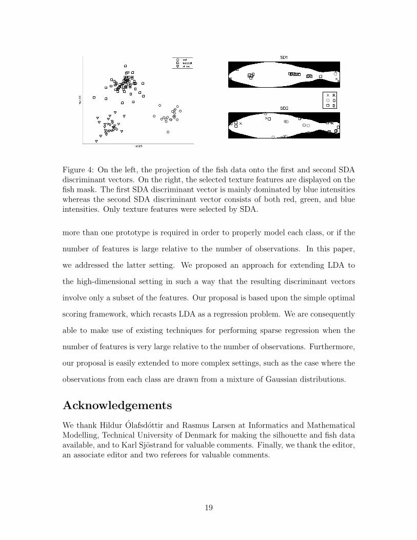
Figure 4: On the left, the projection of the fish data onto the first and second SDAdiscriminant vectors. On the right, the selected texture features are displayed on thefish mask. The first SDA discriminant vector is mainly dominated by blue intensitieswhereas the second SDA discriminant vector consists of both red, green, and blueintensities. Only texture features were selected by SDA.

more than one prototype is required in order to properly model each class, or if the

number of features is large relative to the number of observations. In this paper,

we addressed the latter setting. We proposed an approach for extending LDA to

the high-dimensional setting in such a way that the resulting discriminant vectors

involve only a subset of the features. Our proposal is based upon the simple optimal

scoring framework, which recasts LDA as a regression problem. We are consequently

able to make use of existing techniques for performing sparse regression when the

number of features is very large relative to the number of observations. Furthermore,

our proposal is easily extended to more complex settings, such as the case where the

observations from each class are drawn from a mixture of Gaussian distributions.

Acknowledgements

We thank Hildur Olafsdottir and Rasmus Larsen at Informatics and MathematicalModelling, Technical University of Denmark for making the silhouette and fish dataavailable, and to Karl Sjostrand for valuable comments. Finally, we thank the editor,an associate editor and two referees for valuable comments.

19

References

Barker, M., Rayens, W., 2003. Partial least squares for discrimination. Journal ofChemometrics 17, 166–173.

Bickel, P., Levina, E., 2004. Some theory for Fisher’s linear discriminant function,’naive Bayes’, and some alternatives when there are many more variables thanobservations. Bernoulli 6, 989–1010.

Chun, H., Keles, S., 2010. Sparse partial least squares regression for simultaneousdimension reduction and variable selection. Journal of the Royal Statistical Society- Series B 72 (1), 3–25.

Clemmensen, L., Hansen, M., Ersbøll, B., Frisvad, J., Jan 2007. A method for com-parison of growth media in objective identification of penicillium based on multi-spectral imaging. Journal of Microbiological Methods 69, 249–255.

CRAN, 2009. The comprehensive r archive network.URL http://cran.r-project.org/

Dudoit, S., Fridlyand, J., Speed, T., 2001. Comparison of discrimination methods forthe classification of tumors using gene expression data. J. Amer. Statist. Assoc.96, 1151–1160.

Efron, B., Hastie, T., Johnstore, I., Tibshirani, R., 2004. Least angle regression.Annals of Statistics 32, 407–499.

Friedman, J., 1989. Regularized discriminant analysis. Journal of the American Sta-tistical Association 84, 165–175.

Friedman, J., Hastie, T., Hoefling, H., Tibshirani, R., 2007. Pathwise coordinateoptimization. Annals of Applied Statistics 1, 302–332.

Grosenick, L., Greer, S., Knutson, B., December 2008. Interpretable classifiers forfMRI improve prediction of purchases. IEEE transactions on neural systems andrehabilitation engineering 16 (6), 539–548.

Guo, Y., Hastie, T., Tibshirani, R., 2007. Regularized linear discriminant analysisand its applications in microarrays. Biostatistics 8 (1), 86–100.

Hand, D. J., 2006. Classifier technology and the illusion of progress. Statistical Sci-ence 21 (1), 1–15.

Hastie, T., Buja, A., Tibshirani, R., 1995. Penalized discriminant analysis. The An-nals of Statistics 23 (1), 73–102.

Hastie, T., Tibshirani, R., 1996. Discriminant analysis by Gaussian mixtures. Journalof Royal Statistical Society - Series B 58, 158–176.

20

Hastie, T., Tibshirani, R., Friedman, J., 2009. The Elements of Statistical Learning,2nd Edition. Springer.

Indahl, U., Liland, K., Naes, T., 2009. Canonical partial least squares – a unifiedPLS approach to classification and regression problems. Journal of Chemometrics23, 495–504.

Indahl, U., Martens, H., Naes, T., 2007. From dummy regression to prior probabilitiesin PLS-DA. Journal of Chemometrics 21, 529–536.

Krzanowski, W., Jonathan, P., McCarthy, W., Thomas, M., 1995. Discriminant anal-ysis with singular covariance matrices: methods and applications to spectroscopicdata. Journal of the Royal Statistical Society, Series C 44, 101–115.

Larsen, R., Olafsdottir, H., Ersbøll, B., 2009. Shape and texture based classifica-tion of fish species. In: 16th Scandinavian conference on image analysis. SpringerLecture Notes in Computer Science.

Leng, C., 2008. Sparse optimal scoring for multiclass cancer diagnosis and biomarkerdetection using microarray data. Computational biology and chemistry 32, 417–425.

Thodberg, H. H., Olafsdottir, H., sep 2003. Adding curvature to minimum descriptionlength shape models. In: British Machine Vision Conference, BMVC.

Tibshirani, R., 1996. Regression shrinkage and selection via the lasso. Journal ofRoyal Statistical Society - Series B 58 (No. 1), 267–288.

Tibshirani, R., Hastie, T., Narasimhan, B., Chu, G., 2002. Diagnosis of multiplecancer types by shrunken centroids of gene expression. Proc. Natl. Acad. Sci. 99,6567–6572.

Witten, D., Tibshirani, R., 2011. Penalized classification using fisher’s linear discrim-inant. Journal of the Royal Statistical Society, Series B.

Xu, P., Brock, G., Parrish, R., 2009. Modified linear discriminant analysis approachesfor classification of high-dimensional microarray data. Computational Statisticsand Data Analysis 53, 1674–1687.

Yeoh, E.-J., , et. al, March 2002. Classification, subtype discovery, and prediction ofoutcome in pediatric acute lymphoblastic leukemia by gene expression profiling.Cancer Cell 1, 133–143.

Zou, H., Hastie, T., 2005. Regularization and variable selection via the elastic net.Journal of Royal Statistical Society - Series B 67 (Part 2), 301–320.

Zou, H., Hastie, T., Tibshirani, R., June 2006. Sparse principal component analysis.Journal of Computational and Graphical Statistics 15, 265–286.

21