Span-program-based quantum algorithm for evaluating formulas

Ben W. Reichardt∗ Robert Spalek†

Abstract

We give a quantum algorithm for evaluating formulas over an extended gate set, including all two-and three-bit binary gates (e.g., NAND, 3-majority). The algorithm is optimal on read-once formulasfor which each gate’s inputs are balanced in a certain sense.

The main new tool is a correspondence between a classical linear-algebraic model of computation,“span programs,” and weighted bipartite graphs. A span program’s evaluation corresponds to aneigenvalue-zero eigenvector of the associated graph. A quantum computer can therefore evaluate thespan program by applying spectral estimation to the graph.

For example, the classical complexity of evaluating the balanced ternary majority formula is unknown,and the natural generalization of randomized alpha-beta pruning is known to be suboptimal. In contrast,our algorithm generalizes the optimal quantum AND-OR formula evaluation algorithm and is optimalfor evaluating the balanced ternary majority formula.

1 Introduction

A formula ϕ on gate set S and of size N is a tree with N leaves, such that each internal node is a gatefrom S on its children. The read-once formula evaluation problem is to evaluate ϕ(x) given oracle accessto the input string x = x1x2 . . . xN . An optimal, O(

√N)-query quantum algorithm is known to evaluate

“approximately balanced” formulas over the gates S = AND, OR, NOT [ACR+07]. We extend the gateset S. We develop an optimal quantum algorithm for evaluating balanced, read-once formulas over a gateset S that includes arbitrary three-bit gates, as well as bounded fan-in EQUAL gates and bounded-sizeAND, OR, NOT, PARITY formulas considered as single gates. The correct notion of “balanced” for aformula including different kinds of gates turns out to be “adversary-balanced,” meaning that the inputs toa gate must have exactly equal adversary lower bounds. The definition of “adversary-balanced” formulasalso includes as a special case layered formulas in which all gates at a given depth from the root are of thesame type.

The idea of our algorithm is to consider a weighted graph G(ϕ) obtained by replacing each gate of theformula ϕ with a small gadget subgraph, and possibly also duplicating subformulas. Figure 1 has severalexamples. We relate the evaluation of ϕ to the presence or absence of small-eigenvalue eigenvectors of theweighted adjacency matrix AG(ϕ) that are supported on the root vertex of G(ϕ). The quantum algorithmruns spectral estimation to either detect these eigenvectors or not, and therefore to evaluate ϕ.

As a special case, for example, our algorithm implies:

Theorem 1.1. A balanced ternary majority (MAJ3) formula of depth d, on N = 3d inputs, can be evaluatedby a quantum algorithm with bounded error using O(2d) oracle queries, which is optimal.

The classical complexity of evaluating this formula is known only to lie between Ω((7/3)d) and o((8/3)d),and the previous best quantum algorithm, from [ACR+07], used O(

√5d) queries.

∗School of Computer Science and Institute for Quantum Computing, University of Waterloo. Part of the work conductedwhile at the Institute for Quantum Information, California Institute of Technology, supported by NSF Grants CCF-0524828and PHY-0456720, and by ARO Grant W911NF-05-1-0294. Email: breic@uwaterloo.ca†Google, Inc. Part of the work conducted while at the University of California, Berkeley, supported by NSF Grant CCF-

0524837 and ARO Grant DAAD 19-03-1-0082. Email: spalek@google.com

1

arX

iv:0

710.

2630

v3 [

quan

t-ph

] 1

8 N

ov 2

008

NOT

G(!)!

G(!1)!1 G(¬!1). . . !k . . . . . .G(!k) G(¬!k)

EQUALk

. . .

. . .G(!1) G(!k)!1 !k

ORk MAJ3

!1 !2 !3 G(!3)G(!2)G(!1)

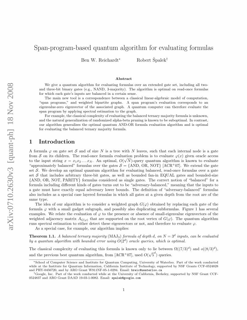
Figure 1: To convert a formula ϕ to the corresponding graph G(ϕ), we recursively apply substitution rulesstarting at the root to convert each gate into a gadget subgraph. Some of the rules are shown here, exceptwith the edge weights not indicated. The dangling edges at the top and bottom of each gadget are the inputedges and output edge, respectively. To compose two gates, the output edge of one is identified with aninput edge of the next (see Figure 4).

The graph gadgets themselves are derived from “span programs” [KW93]. Span programs have been usedin classical complexity theory to prove lower bounds on formula size [KW93, BGW99] and monotone spanprograms are related to linear secret-sharing schemes [BGP96]. (Most, though not all [ABO99], applicationsare over finite fields, whereas we use the definition over C.) We will only use compositions of constant-sizespan programs, but it is interesting to speculate that larger span programs could directly give useful newquantum algorithms.

Classical and quantum background The formula evaluation problem has been well-studied in theclassical computer model. Classically, the case S = NAND is best understood. A formula with only NANDgates is equivalent to one with alternating levels of AND and OR gates, a so-called “AND-OR formula,”also known as a two-player game tree. One can compute the value of a balanced binary AND-OR formulawith zero error in expected time O(N log2[(1+

√33)/4]) = O(N0.754) [Sni85, SW86], and this is optimal even

for bounded-error algorithms [San95]. However, the complexity of evaluating balanced AND-OR formulasgrows with the degree of the gates. For example, in the extreme case of a single OR gate of degree N ,the complexity is Θ(N). The complexity of evaluating AND-OR formulas that are not “well-balanced” isunknown.

If we allow the use of a quantum computer with coherent oracle access to the input, however, then thesituation is much simpler; between Ω(

√N) and N

12 +o(1) queries are necessary and sufficient to evaluate

any AND, OR, NOT formula with bounded error. In one extreme case, Grover search [Gro96, Gro02]evaluates an OR gate of degree N using O(

√N) oracle queries and O(

√N log logN) time. In the other

extreme case, Farhi, Goldstone and Gutmann recently devised a breakthrough algorithm for evaluatingthe depth-log2N balanced binary AND-OR formula in O(

√N) time in the unconventional Hamiltonian

oracle model [FGG07]. Ambainis [Amb07] improved this to O(√N)-queries in the standard query model.

Childs, Reichardt, Spalek and Zhang [CRSZ07] gave an O(√N)-query algorithm for evaluating balanced or

“approximately balanced” formulas, and extended the algorithm to arbitrary AND, OR, NOT formulaswith N

12 +o(1) queries, and also N

12 +o(1) time after a preprocessing step. (Ref. [ACR+07] contains the merged

results of [Amb07, CRSZ07].)This paper shows other nice features of the formula evaluation problem in the quantum computer model.

Classically, with the exception of NAND, NOR and a few trivial cases like PARITY, most gatesets are poorly understood. In 1986, Boppana asked the complexity of evaluating the balanced, depth-dternary majority (MAJ3) function [SW86], and today the complexity is only known to lie between Ω((7/3)d)and O((2.6537 . . .)d) [JKS03]. In particular, the naıve generalization of randomized alpha-beta pruning—recursively evaluate two random immediate subformulas and then the third if they disagree—runs in expectedtime O((8/3)d) and is suboptimal. This suggests that the balanced ternary majority function is significantlydifferent from the balanced k-ary NAND function, for which randomized alpha-beta pruning is known tobe optimal. In contrast, we show that the optimal quantum algorithm of [CRSZ07] does extend to givean optimal O(2d)-query algorithm for evaluating the balanced ternary majority formula. Moreover, thealgorithm also generalizes to a significantly larger gate set S.

2

Organization We introduce span programs and explain their correspondence to weighted bipartite graphsin Section 2. The correspondence involves considering parts of a span program P as the weighted adjacencymatrix for a corresponding graph GP . We prove that the eigenvalue-zero eigenvectors of this adjacencymatrix evaluate P (Theorem 2.5). This theorem provides useful intuition.

We develop a quantitative version of Theorem 2.5 in Section 3. We lower-bound the overlap of theeigenvalue-zero eigenvector with a known starting state. This lower-bound will imply completeness of ourquantum algorithm. To show soundness of the algorithm, we also analyze small-eigenvalue eigenvectorsin order to prove a spectral gap around zero. Essentially, we solve the eigenvalue equations in terms ofthe eigenvalue λ, and expand a series around λ = 0. The results for small-eigenvalue and eigenvalue-zeroeigenvectors are closely related, and we unify them using a measure we term “span program witness size.”The details of the proofs from this section are in Appendix A.

Section 4 applies the span program framework to the formula evaluation problem. Theorem 4.7 isour general result, an optimal quantum algorithm for evaluating formulas that are over the gate set S ofDefinition 4.1, and that are adversary-balanced (Definition 4.5). The proof of Theorem 4.7 has three parts.First, in Section 4.2, we display an optimal span program for each of the gates in S. Second, we compose thespan programs for the individual gates to obtain a span program for the full formula ϕ. This is equivalent tojoining together the gadget graphs described in Figure 1 to obtain a graph G(ϕ). We combine the spectralanalyses of the individual span programs to analyze the spectrum of G(ϕ) (Theorem 4.16). Finally, thisanalysis straightforwardly leads to a quantum algorithm based on phase estimation of a quantum walk onG(ϕ), in Section 4.4.

Section 5 concludes with a discussion of some extensions to the algorithm.

2 Span programs and eigenvalue-zero graph eigenvectors

A span program P is a certain linear-algebraic way of specifying a function fP . For details on span programsapplied in classical complexity theory, we can still recommend the original reference [KW93] as well as, e.g.,the more recent [GP03].

Definition 2.1 (Span program). A span program P consists of a nonzero “target” vector t in a vector spaceover C, together with “grouped input” vectors vj : j ∈ J. Each vj is labeled with a subset Xj of the literalsx1, x1, . . . , xn, xn. To P corresponds a boolean function fP : 0, 1n → 0, 1; defined by fP (x) = 1 (i.e.,true) if and only if there exists a linear combination

∑j ajvj = t such that aj = 0 if any of the literals in

Xj evaluates to zero (i.e., false).

Example 2.2. For example, the span program

XJ = (x1 x2 x3 )

t =

(1), vJ =

(1√3

1√3

1√3

)0 1 e2πi/2 e−2πi/3

computes the MAJ3 function. Indeed, at least two of the vj must have nonzero coefficient in any linearcombination equaling the target t. Of course, the second row of (v1 v2 v3) could be any (α β γ) withα, β, γ distinct and nonzero, and the span program would still compute MAJ3. This specific setting is usedto optimize the running time of the quantum algorithm (Claim 4.9).

In this section, we will show that by viewing a span program P as the weighted adjacency matrix AGP ofa certain graph GP , the true/false evaluation of P on input x corresponds to the existence or nonexistenceof an eigenvalue-zero eigenvector of AGP (x) supported on a distinguished output node (Theorem 2.5).

In turn, this will imply that writing a span program P for a function f immediately gives a quantumalgorithm for evaluating f , or for evaluating formulas including f as a gate (Section 4). The algorithmworks by spectral estimation on AGP (x). Its running time depends on the span program’s “witness size”(Section 3). For example, if fP (x) is true, then the witness size is essentially the shortest squared length ofany witness vector (aj)j∈J in Definition 2.1.

3

bI|J|

a|J|. . .

. . .

a1

bI1

bCaO

bO

!"#$ !"#$

! "# $

. . . . . .

AGP =

aO aJ︷︸︸︷1 AOJ

bO

0:0

ACJ

bC

0:0

AIJ

bI

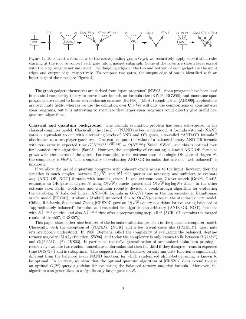
Figure 2: The bipartite graph GP corresponding to span program P (the output edge is (aO, bO), while thegrouped inputs are a1, . . . , a|J|).

Remark 2.3. Let us clarify a few points in Definition 2.1.

1. It is convenient, but nonstandard, to allow grouped inputs, i.e., literal subsets Xj possibly with |Xj | > 1,instead of just single literals, to label the columns. A grouped input j can be thought of as evaluatingthe AND of all literals in Xj. A span program P with some |Xj | > 1 can be expanded out so that all|Xj | ≤ 1, without increasing

∑j |Xj |, known as the size of P .

2. It is sometimes convenient to allow Xj = ∅. In this case, vector vj is always available to use in thelinear combination; grouped input j evaluates to true always. However, such vectors can be eliminatedfrom P without increasing the size [KW93, Theorem 7].

3. By a basis change, one can always adjust the target vector t to (1, 0, 0, . . . , 0).

2.1 Span program as an adjacency matrix

A span program P with target vector t = (1, 0, . . . , 0) corresponds to a certain weighted bipartite graph.Notation: For an index sequence H = (h1, . . . , h|H|) and a set of variables ah, let aH = (ah1 , . . . , ah|H|).

For example, vJ denotes the sequence of grouped input vectors. It will be convenient to define several moreindex sequences: O (“output”), C (“constraints”) and I (“inputs”). Let O and C together index thecoordinates of the vector space, with O = 1 being the first coordinate, and C the remainder. Let Ij indexXj for each j ∈ J , and let I =

⋃j∈J Ij a disjoint union so |I| = size(P ).

We will construct a graph GP on |I| + |J | + |C| + 2|O| vertices. Writing the grouped input vectors outas the columns of a matrix, let

(AOJACJ

)=∑j∈J |vj〉〈j|; AOJ is a 1 × |J | matrix row, and ACJ is a |C| × |J |

matrix. Let AIJ =∑j∈J,i∈Ij |i〉〈j|; AIJ encodes P ’s grouped inputs. Now consider the bipartite graph GP

of Figure 2, the upper right block of whose weighted Hermitian adjacency matrix is AGP . (The adjacencymatrix is block off-diagonal because the graph is bipartite.) The edges (aj , bi) for j ∈ J and i ∈ Ij are “inputedges,” while (aO, bO) is the “output edge.” The input and output edges all have weight one. The weightsof edges (bO, aj) for j ∈ J are given by AOJ (the first coordinates of the grouped input vectors vJ), whilethe weights of edges (bc, aj) for c ∈ C, j ∈ J are given by ACJ (the remaining coordinates of vJ).

Example 2.4. For the MAJ3 span program of Example 2.2, |C| = 1, |I| = |J | = 3, the graph GP is shownin Figure 1, and the matrix AGP is

1 1√3

1√3

1√3

0 1 e2πi/3 e−2πi/3

0 1 0 00 0 1 00 0 0 1

.

4

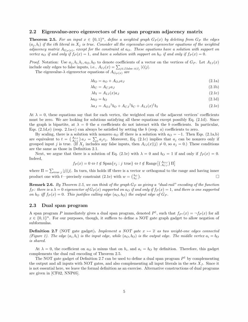
2.2 Eigenvalue-zero eigenvectors of the span program adjacency matrix

Theorem 2.5. For an input x ∈ 0, 1n, define a weighted graph GP (x) by deleting from GP the edges(aj , bi) if the ith literal in Xj is true. Consider all the eigenvalue-zero eigenvector equations of the weightedadjacency matrix AGP (x), except for the constraint at aO. These equations have a solution with support onvertex aO if and only if fP (x) = 1, and have a solution with support on bO if and only if fP (x) = 0.

Proof. Notation: Use aj , bi, bc, aO, bO to denote coefficients of a vector on the vertices of GP . Let AIJ(x)include only edges to false inputs, i.e., AIJ(x) =

∑j∈J,false i∈Ij |i〉〈j|.

The eigenvalue-λ eigenvector equations of AGP (x) are

λbO = aO +AOJaJ (2.1a)λbC = ACJaJ (2.1b)λbI = AIJ(x)aJ (2.1c)λaO = bO (2.1d)

λaJ = AOJ†bO +ACJ

†bC +AIJ(x)†bI (2.1e)

At λ = 0, these equations say that for each vertex, the weighted sum of the adjacent vertices’ coefficientsmust be zero. We are looking for solutions satisfying all these equations except possibly Eq. (2.1d). Sincethe graph is bipartite, at λ = 0 the a coefficients do not interact with the b coefficients. In particular,Eqs. (2.1d,e) (resp. 2.1a-c) can always be satisfied by setting the b (resp. a) coefficients to zero.

By scaling, there is a solution with nonzero aO iff there is a solution with aO = −1. Then Eqs. (2.1a,b)are equivalent to t =

(AOJACJ

)aJ =

∑j ajvj . Moreover, Eq. (2.1c) implies that aj can be nonzero only if

grouped input j is true. (If Xj includes any false inputs, then AIJ(x)|j〉 6= 0, so aj = 0.) These conditionsare the same as those in Definition 2.1.

Next, we argue that there is a solution of Eq. (2.1e) with λ = 0 and bO = 1 if and only if fP (x) = 0.Indeed,

fP (x) = 0⇔ t /∈ Spanvj : j true ⇔ t /∈ Range[(AOJACJ

)Π]

where Π =∑

true j |j〉〈j|. In turn, this holds iff there is a vector w orthogonal to the range and having innerproduct one with t—precisely constraint (2.1e) with w =

(bObC

).

Remark 2.6. By Theorem 2.5, we can think of the graph GP as giving a “dual-rail” encoding of the functionfP : there is a λ = 0 eigenvector of GP (x) supported on aO if and only if fP (x) = 1, and there is one supportedon bO iff fP (x) = 0. This justifies calling edge (aO, bO) the output edge of GP .

2.3 Dual span program

A span program P immediately gives a dual span program, denoted P †, such that fP †(x) = ¬fP (x) for allx ∈ 0, 1n. For our purposes, though, it suffices to define a NOT gate graph gadget to allow negation ofsubformulas.

Definition 2.7 (NOT gate gadget). Implement a NOT gate x 7→ x as two weight-one edges connected(Figure 1). The edge (ai, bi) is the input edge, while (aO, bO) is the output edge. The middle vertex ai = bOis shared.

At λ = 0, the coefficient on aO is minus that on bi, and ai = bO by definition. Therefore, this gadgetcomplements the dual rail encoding of Theorem 2.5.

The NOT gate gadget of Definition 2.7 can be used to define a dual span program P † by complementingthe output and all inputs with NOT gates, and also complementing all input literals in the sets XJ . Since itis not essential here, we leave the formal definition as an exercise. Alternative constructions of dual programsare given in [CF02, NNP05].

5

x4x1 x2 x3 x5

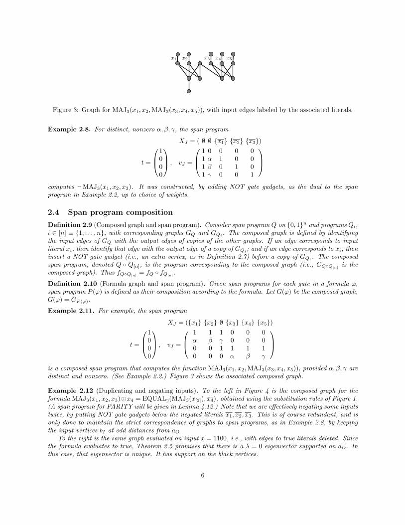
Figure 3: Graph for MAJ3(x1, x2,MAJ3(x3, x4, x5)), with input edges labeled by the associated literals.

Example 2.8. For distinct, nonzero α, β, γ, the span program

XJ = ( ∅ ∅ x1 x2 x3)

t =

1 , vJ =

1 0 0 0 0 0 1 α 1 0 00 1 β 0 1 00 1 γ 0 0 1

computes ¬MAJ3(x1, x2, x3). It was constructed, by adding NOT gate gadgets, as the dual to the spanprogram in Example 2.2, up to choice of weights.

2.4 Span program composition

Definition 2.9 (Composed graph and span program). Consider span program Q on 0, 1n and programs Qi,i ∈ [n] ≡ 1, . . . , n, with corresponding graphs GQ and GQi . The composed graph is defined by identifyingthe input edges of GQ with the output edges of copies of the other graphs. If an edge corresponds to inputliteral xi, then identify that edge with the output edge of a copy of GQi ; and if an edge corresponds to xi, theninsert a NOT gate gadget (i.e., an extra vertex, as in Definition 2.7) before a copy of GQi . The composedspan program, denoted Q Q[n], is the program corresponding to the composed graph (i.e., GQQ[n] is thecomposed graph). Thus fQQ[n] = fQ fQ[n] .

Definition 2.10 (Formula graph and span program). Given span programs for each gate in a formula ϕ,span program P (ϕ) is defined as their composition according to the formula. Let G(ϕ) be the composed graph,G(ϕ) = GP (ϕ).

Example 2.11. For example, the span program

XJ = (x1 x2 ∅ x3 x4 x5)

t =

1 , vJ =

1 1 1 0 0 0 0 α β γ 0 0 0

0 0 0 1 1 1 10 0 0 0 α β γ

is a composed span program that computes the function MAJ3(x1, x2,MAJ3(x3, x4, x5)), provided α, β, γ aredistinct and nonzero. (See Example 2.2.) Figure 3 shows the associated composed graph.

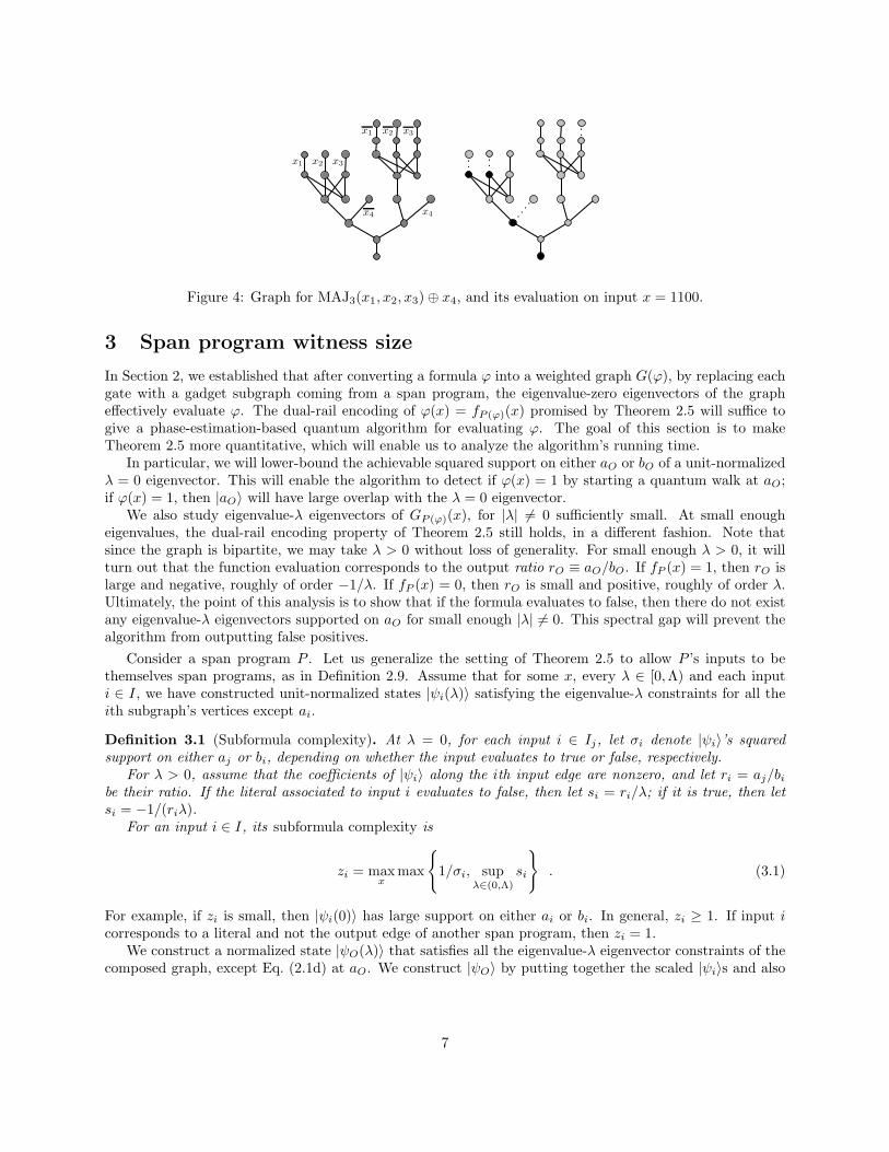
Example 2.12 (Duplicating and negating inputs). To the left in Figure 4 is the composed graph for theformula MAJ3(x1, x2, x3)⊕x4 = EQUAL2(MAJ3(x[3]), x4), obtained using the substitution rules of Figure 1.(A span program for PARITY will be given in Lemma 4.12.) Note that we are effectively negating some inputstwice, by putting NOT gate gadgets below the negated literals x1, x2, x3. This is of course redundant, and isonly done to maintain the strict correspondence of graphs to span programs, as in Example 2.8, by keepingthe input vertices bI at odd distances from aO.

To the right is the same graph evaluated on input x = 1100, i.e., with edges to true literals deleted. Sincethe formula evaluates to true, Theorem 2.5 promises that there is a λ = 0 eigenvector supported on aO. Inthis case, that eigenvector is unique. It has support on the black vertices.

6

x4

x1 x2 x3

x4

x1 x2 x3

Figure 4: Graph for MAJ3(x1, x2, x3)⊕ x4, and its evaluation on input x = 1100.

3 Span program witness size

In Section 2, we established that after converting a formula ϕ into a weighted graph G(ϕ), by replacing eachgate with a gadget subgraph coming from a span program, the eigenvalue-zero eigenvectors of the grapheffectively evaluate ϕ. The dual-rail encoding of ϕ(x) = fP (ϕ)(x) promised by Theorem 2.5 will suffice togive a phase-estimation-based quantum algorithm for evaluating ϕ. The goal of this section is to makeTheorem 2.5 more quantitative, which will enable us to analyze the algorithm’s running time.

In particular, we will lower-bound the achievable squared support on either aO or bO of a unit-normalizedλ = 0 eigenvector. This will enable the algorithm to detect if ϕ(x) = 1 by starting a quantum walk at aO;if ϕ(x) = 1, then |aO〉 will have large overlap with the λ = 0 eigenvector.

We also study eigenvalue-λ eigenvectors of GP (ϕ)(x), for |λ| 6= 0 sufficiently small. At small enougheigenvalues, the dual-rail encoding property of Theorem 2.5 still holds, in a different fashion. Note thatsince the graph is bipartite, we may take λ > 0 without loss of generality. For small enough λ > 0, it willturn out that the function evaluation corresponds to the output ratio rO ≡ aO/bO. If fP (x) = 1, then rO islarge and negative, roughly of order −1/λ. If fP (x) = 0, then rO is small and positive, roughly of order λ.Ultimately, the point of this analysis is to show that if the formula evaluates to false, then there do not existany eigenvalue-λ eigenvectors supported on aO for small enough |λ| 6= 0. This spectral gap will prevent thealgorithm from outputting false positives.

Consider a span program P . Let us generalize the setting of Theorem 2.5 to allow P ’s inputs to bethemselves span programs, as in Definition 2.9. Assume that for some x, every λ ∈ [0,Λ) and each inputi ∈ I, we have constructed unit-normalized states |ψi(λ)〉 satisfying the eigenvalue-λ constraints for all theith subgraph’s vertices except ai.

Definition 3.1 (Subformula complexity). At λ = 0, for each input i ∈ Ij, let σi denote |ψi〉’s squaredsupport on either aj or bi, depending on whether the input evaluates to true or false, respectively.

For λ > 0, assume that the coefficients of |ψi〉 along the ith input edge are nonzero, and let ri = aj/bibe their ratio. If the literal associated to input i evaluates to false, then let si = ri/λ; if it is true, then letsi = −1/(riλ).

For an input i ∈ I, its subformula complexity is

zi = maxx

max

1/σi, sup

λ∈(0,Λ)

si

. (3.1)

For example, if zi is small, then |ψi(0)〉 has large support on either ai or bi. In general, zi ≥ 1. If input icorresponds to a literal and not the output edge of another span program, then zi = 1.

We construct a normalized state |ψO(λ)〉 that satisfies all the eigenvalue-λ eigenvector constraints of thecomposed graph, except Eq. (2.1d) at aO. We construct |ψO〉 by putting together the scaled |ψi〉s and also

7

assigning coefficients to the vertices in GP . Similarly to Eq. (3.1), define

zO(x) = max

1/σO, sup

λ∈(0,Λ)

sO

, (3.2)

where σO is the squared support of |ψO(0)〉 on aO or bO, and, for λ > 0, sO is −1/(rOλ) or rO/λ if f(x) istrue or false, respectively. We will relate zO = maxx zO(x) to the input complexities zI (Theorem 3.7).

First of all, notice that if |Ij | > 1, then several of the input subgraphs share the vertex aj . They mustbe scaled so that their coefficients at aj all match, motivating the following definition.

Definition 3.2. The grouped input complexity of j ∈ J on input x is

zj(x) =

max∑

i∈Ij zi, 1

if j evaluates to true(∑false i ∈ Ij z

−1i

)−1

otherwise(3.3)

Recall that grouped input j evaluates to true iff all inputs in Ij are true. (In the first case, we take themaximum with 1 to handle the case Ij = ∅.)

When j is false, some input i ∈ Ij is false, so the coefficient at aj must be set to zero at λ = 0. However, foreach false i ∈ Ij , |ψi〉 can be scaled arbitrarily. The definition in Eq. (3.3) comes from choosing scale factorsfi in order to maximize the sum of the scaled coefficients on the vertices bi, under the constraint that thetotal norm be one,

∑i∈Ij |fi|

2 = 1.A few more definitions are needed to state Theorem 3.7.

Definition 3.3 (Asymptotic notation). Let a . b mean that there exist constants c1, c2 such that a ≤c1 + b(1 + c2|λ|maxi zi).

Definition 3.4 (Matrix notations). For a given input x, let Π(x) =∑

true j |j〉〈j| a projection onto thetrue grouped inputs, Π(x) = 1 − Π(x), and z(x) =

∑j zj(x)|j〉〈j| a diagonal matrix of the grouped input

complexities. To simplify equations, we will generally leave implicit the dependence on x, writing Π, Π andz. Let A =

(AOJACJ

)=∑j |vj〉〈j| with columns the vectors |vj〉.

Definition 3.5 (Moore-Penrose pseudoinverse). For a matrix M , let M+ denote its Moore-Penrose pseu-doinverse. If the singular-value decomposition of M is M =

∑kmk|k〉〈k′| with all mk > 0 and for sets

of orthonormal vectors |k〉 and |k′〉, then M+ =∑km−1k |k′〉〈k|. Note that MM+ =

∑k |k〉〈k| is the

projection onto M ’s range.

Definition 3.6 (Span program witness size). For span program P and input subformula complexities zI ,the witness size of P is wsize(P ) = maxx wsize(P, x), where for an input x, wsize(P, x) is defined as follows:

• If fP (x) = 1, then |t〉 ∈ Range(AΠ), so there is a witness |w〉 ∈ C|J| satisfying AΠ|w〉 = |t〉. Thenwsize(P, x) is the minimum squared length, weighted by z(x)1/2, of any such witness:

wsize(P, x) = min|w〉:AΠ|w〉=|t〉

‖z1/2|w〉‖2 (3.4)

= ‖(AΠz−1/2)+|t〉‖2 .

• If fP (x) = 0, then |t〉 /∈ Range(AΠ). Therefore there is a witness |w′〉 ∈ C|C|+1 satisfying 〈t|w′〉 = 1and ΠA†|w′〉 = 0. Then

wsize(P, x) = min|w′〉:〈t|w′〉=1

ΠA†|w′〉=0

‖z1/2A†|w′〉‖2 (3.5)

= ‖(1 + (Π(Az1/2)+Az1/2 − 1)+Π

)(Az1/2)+|t〉‖−2 ,

the inverse squared length of the projection of (Az1/2)+|t〉 onto the intersection of Π and Range(z1/2A†).

8

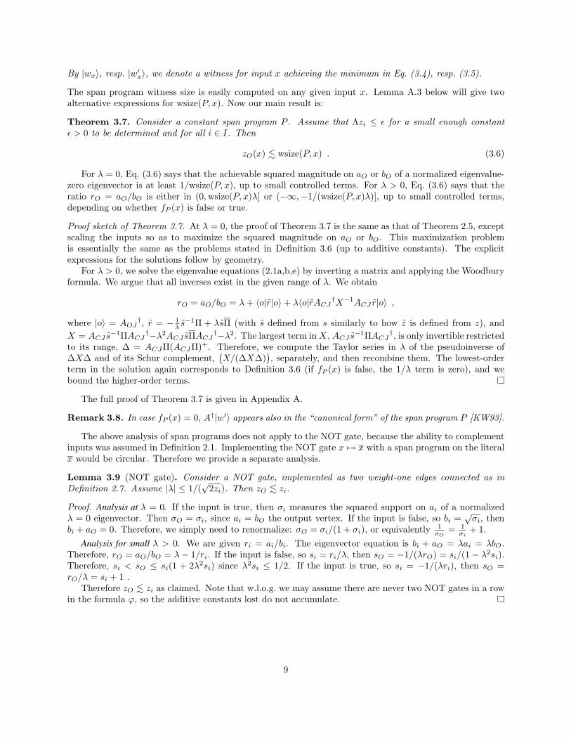
By |wx〉, resp. |w′x〉, we denote a witness for input x achieving the minimum in Eq. (3.4), resp. (3.5).

The span program witness size is easily computed on any given input x. Lemma A.3 below will give twoalternative expressions for wsize(P, x). Now our main result is:

Theorem 3.7. Consider a constant span program P . Assume that Λzi ≤ ε for a small enough constantε > 0 to be determined and for all i ∈ I. Then

zO(x) . wsize(P, x) . (3.6)

For λ = 0, Eq. (3.6) says that the achievable squared magnitude on aO or bO of a normalized eigenvalue-zero eigenvector is at least 1/wsize(P, x), up to small controlled terms. For λ > 0, Eq. (3.6) says that theratio rO = aO/bO is either in (0,wsize(P, x)λ] or (−∞,−1/(wsize(P, x)λ)], up to small controlled terms,depending on whether fP (x) is false or true.

Proof sketch of Theorem 3.7. At λ = 0, the proof of Theorem 3.7 is the same as that of Theorem 2.5, exceptscaling the inputs so as to maximize the squared magnitude on aO or bO. This maximization problemis essentially the same as the problems stated in Definition 3.6 (up to additive constants). The explicitexpressions for the solutions follow by geometry.

For λ > 0, we solve the eigenvalue equations (2.1a,b,e) by inverting a matrix and applying the Woodburyformula. We argue that all inverses exist in the given range of λ. We obtain

rO = aO/bO = λ+ 〈o|r|o〉+ λ〈o|rACJ †X−1ACJ r|o〉 ,

where |o〉 = AOJ†, r = − 1

λ s−1Π + λsΠ (with s defined from s similarly to how z is defined from z), and

X = ACJ s−1ΠACJ †−λ2ACJ sΠACJ †−λ2. The largest term inX, ACJ s−1ΠACJ †, is only invertible restricted

to its range, ∆ = ACJΠ(ACJΠ)+. Therefore, we compute the Taylor series in λ of the pseudoinverse of∆X∆ and of its Schur complement,

(X/(∆X∆)

), separately, and then recombine them. The lowest-order

term in the solution again corresponds to Definition 3.6 (if fP (x) is false, the 1/λ term is zero), and webound the higher-order terms.

The full proof of Theorem 3.7 is given in Appendix A.

Remark 3.8. In case fP (x) = 0, A†|w′〉 appears also in the “canonical form” of the span program P [KW93].

The above analysis of span programs does not apply to the NOT gate, because the ability to complementinputs was assumed in Definition 2.1. Implementing the NOT gate x 7→ x with a span program on the literalx would be circular. Therefore we provide a separate analysis.

Lemma 3.9 (NOT gate). Consider a NOT gate, implemented as two weight-one edges connected as inDefinition 2.7. Assume |λ| ≤ 1/(

√2zi). Then zO . zi.

Proof. Analysis at λ = 0. If the input is true, then σi measures the squared support on ai of a normalizedλ = 0 eigenvector. Then σO = σi, since ai = bO the output vertex. If the input is false, so bi =

√σi, then

bi + aO = 0. Therefore, we simply need to renormalize: σO = σi/(1 + σi), or equivalently 1σO

= 1σi

+ 1.Analysis for small λ > 0. We are given ri = ai/bi. The eigenvector equation is bi + aO = λai = λbO.

Therefore, rO = aO/bO = λ− 1/ri. If the input is false, so si = ri/λ, then sO = −1/(λrO) = si/(1− λ2si).Therefore, si < sO ≤ si(1 + 2λ2si) since λ2si ≤ 1/2. If the input is true, so si = −1/(λri), then sO =rO/λ = si + 1 .

Therefore zO . zi as claimed. Note that w.l.o.g. we may assume there are never two NOT gates in a rowin the formula ϕ, so the additive constants lost do not accumulate.

9

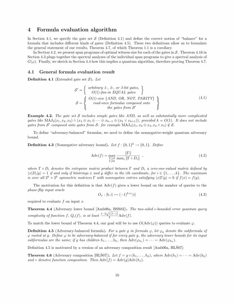
4 Formula evaluation algorithm

In Section 4.1, we specify the gate set S (Definition 4.1) and define the correct notion of “balance” for aformula that includes different kinds of gates (Definition 4.5). These two definitions allow us to formulatethe general statement of our results, Theorem 4.7, of which Theorem 1.1 is a corollary.

In Section 4.2, we present span programs of optimal witness size for each of the gates in S. Theorem 4.16 inSection 4.3 plugs together the spectral analyses of the individual span programs to give a spectral analysis ofG(ϕ). Finally, we sketch in Section 4.4 how this implies a quantum algorithm, therefore proving Theorem 4.7.

4.1 General formula evaluation result

Definition 4.1 (Extended gate set S). Let

S ′ =

arbitrary 1-, 2-, or 3-bit gates,O(1)-fan-in EQUAL gates

S =

O(1)-size AND, OR, NOT, PARITYread-once formulas composed onto

the gates from S ′

(4.1)

Example 4.2. The gate set S includes simple gates like AND, as well as substantially more complicatedgates like MAJ3(x1, x2, x3) ∧ (x4 ⊕ x5 ⊕ · · · ⊕ xk−1 ⊕ (xk ∨ xk+1)), provided k = O(1). It does not includegates from S ′ composed onto gates from S: for example MAJ3(x1, x2 ⊕ x3, x4 ∧ x5) /∈ S.

To define “adversary-balanced” formulas, we need to define the nonnegative-weight quantum adversarybound.

Definition 4.3 (Nonnegative adversary bound). Let f : 0, 1k → 0, 1. Define

Adv(f) = maxΓ≥0Γ6=0

‖Γ‖maxi ‖Γ Di‖

, (4.2)

where Γ Di denotes the entrywise matrix product between Γ and Di a zero-one-valued matrix defined by〈x|Di|y〉 = 1 if and only if bitstrings x and y differ in the ith coordinate, for i ∈ 1, . . . , k. The maximumis over all 2k × 2k symmetric matrices Γ with nonnegative entries satisfying 〈x|Γ|y〉 = 0 if f(x) = f(y).

The motivation for this definition is that Adv(f) gives a lower bound on the number of queries to thephase-flip input oracle

Ox : |b, i〉 7→ (−1)b·xi |i〉 (4.3)

required to evaluate f on input x.

Theorem 4.4 (Adversary lower bound [Amb06a, BSS03]). The two-sided ε-bounded error quantum query

complexity of function f , Qε(f), is at least 1−2√ε(1−ε)2 Adv(f).

To match the lower bound of Theorem 4.4, our goal will be to use O(Adv(ϕ)) queries to evaluate ϕ.

Definition 4.5 (Adversary-balanced formula). For a gate g in formula ϕ, let ϕg denote the subformula ofϕ rooted at g. Define ϕ to be adversary-balanced if for every gate g, the adversary lower bounds for its inputsubformulas are the same; if g has children h1, . . . , hk, then Adv(ϕh1) = · · · = Adv(ϕhk).

Definition 4.5 is motivated by a version of an adversary composition result [Amb06a, HLS07]:

Theorem 4.6 (Adversary composition [HLS07]). Let f = g (h1, . . . , hk), where Adv(h1) = · · · = Adv(hk)and denotes function composition. Then Adv(f) = Adv(g)Adv(h1).

10

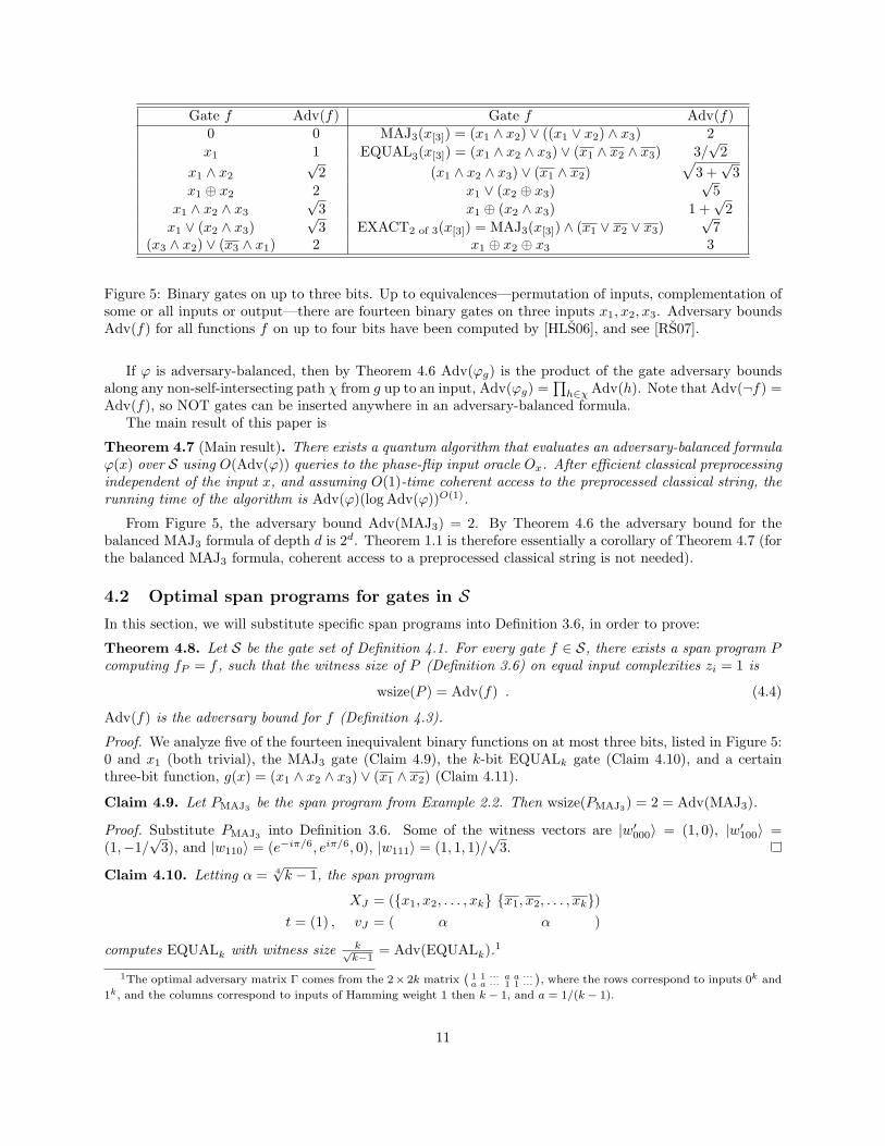
Gate f Adv(f) Gate f Adv(f)0 0 MAJ3(x[3]) = (x1 ∧ x2) ∨ ((x1 ∨ x2) ∧ x3) 2x1 1 EQUAL3(x[3]) = (x1 ∧ x2 ∧ x3) ∨ (x1 ∧ x2 ∧ x3) 3/

√2

x1 ∧ x2

√2 (x1 ∧ x2 ∧ x3) ∨ (x1 ∧ x2)

√3 +√

3x1 ⊕ x2 2 x1 ∨ (x2 ⊕ x3)

√5

x1 ∧ x2 ∧ x3

√3 x1 ⊕ (x2 ∧ x3) 1 +

√2

x1 ∨ (x2 ∧ x3)√

3 EXACT2 of 3(x[3]) = MAJ3(x[3]) ∧ (x1 ∨ x2 ∨ x3)√

7(x3 ∧ x2) ∨ (x3 ∧ x1) 2 x1 ⊕ x2 ⊕ x3 3

Figure 5: Binary gates on up to three bits. Up to equivalences—permutation of inputs, complementation ofsome or all inputs or output—there are fourteen binary gates on three inputs x1, x2, x3. Adversary boundsAdv(f) for all functions f on up to four bits have been computed by [HLS06], and see [RS07].

If ϕ is adversary-balanced, then by Theorem 4.6 Adv(ϕg) is the product of the gate adversary boundsalong any non-self-intersecting path χ from g up to an input, Adv(ϕg) =

∏h∈χ Adv(h). Note that Adv(¬f) =

Adv(f), so NOT gates can be inserted anywhere in an adversary-balanced formula.The main result of this paper is

Theorem 4.7 (Main result). There exists a quantum algorithm that evaluates an adversary-balanced formulaϕ(x) over S using O(Adv(ϕ)) queries to the phase-flip input oracle Ox. After efficient classical preprocessingindependent of the input x, and assuming O(1)-time coherent access to the preprocessed classical string, therunning time of the algorithm is Adv(ϕ)(log Adv(ϕ))O(1).

From Figure 5, the adversary bound Adv(MAJ3) = 2. By Theorem 4.6 the adversary bound for thebalanced MAJ3 formula of depth d is 2d. Theorem 1.1 is therefore essentially a corollary of Theorem 4.7 (forthe balanced MAJ3 formula, coherent access to a preprocessed classical string is not needed).

4.2 Optimal span programs for gates in SIn this section, we will substitute specific span programs into Definition 3.6, in order to prove:

Theorem 4.8. Let S be the gate set of Definition 4.1. For every gate f ∈ S, there exists a span program Pcomputing fP = f , such that the witness size of P (Definition 3.6) on equal input complexities zi = 1 is

wsize(P ) = Adv(f) . (4.4)

Adv(f) is the adversary bound for f (Definition 4.3).

Proof. We analyze five of the fourteen inequivalent binary functions on at most three bits, listed in Figure 5:0 and x1 (both trivial), the MAJ3 gate (Claim 4.9), the k-bit EQUALk gate (Claim 4.10), and a certainthree-bit function, g(x) = (x1 ∧ x2 ∧ x3) ∨ (x1 ∧ x2) (Claim 4.11).

Claim 4.9. Let PMAJ3 be the span program from Example 2.2. Then wsize(PMAJ3) = 2 = Adv(MAJ3).

Proof. Substitute PMAJ3 into Definition 3.6. Some of the witness vectors are |w′000〉 = (1, 0), |w′100〉 =(1,−1/

√3), and |w110〉 = (e−iπ/6, eiπ/6, 0), |w111〉 = (1, 1, 1)/

√3.

Claim 4.10. Letting α = 4√k − 1, the span program

XJ = (x1, x2, . . . , xk x1, x2, . . . , xk)t = (1) , vJ = ( α α )

computes EQUALk with witness size k√k−1

= Adv(EQUALk).1

1The optimal adversary matrix Γ comes from the 2× 2k matrix`

1 1 ··· a a ···a a ··· 1 1 ···

´, where the rows correspond to inputs 0k and

1k, and the columns correspond to inputs of Hamming weight 1 then k − 1, and a = 1/(k − 1).

11

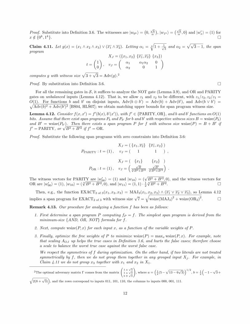
Proof. Substitute into Definition 3.6. The witnesses are |w0k〉 =(0,√kα

), |w1k〉 =

(√kα , 0

)and |w′x〉 = (1) for

x /∈ 0k, 1k.

Claim 4.11. Let g(x) = (x1 ∧ x2 ∧ x3) ∨ (x1 ∧ x2). Letting α1 = 4

√1 + 1√

3and α2 =

√√3− 1, the span

programXJ = (x1, x2 x1, x2 x3)

t =(

1), vJ =

(α1 α1α2 0

)0 α2 0 1

computes g with witness size√

3 +√

3 = Adv(g).2

Proof. By substitution into Definition 3.6.

For all the remaining gates in S, it suffices to analyze the NOT gate (Lemma 3.9), and OR and PARITYgates on unbalanced inputs (Lemma 4.12). That is, we allow z1 and z2 to be different, with z1/z2, z2/z1 =O(1). For functions b and b′ on disjoint inputs, Adv(b ⊕ b′) = Adv(b) + Adv(b′), and Adv(b ∨ b′) =√

Adv(b)2 + Adv(b′)2 [BS04, HLS07]; we obtain matching upper bounds for span program witness size.

Lemma 4.12. Consider f(x, x′) = f ′(b(x), b′(x′)), with f ′ ∈ PARITY,OR, and b and b′ functions on O(1)bits. Assume that there exist span programs Pb and Pb′ for b and b′ with respective witness sizes B = wsize(Pb)and B′ = wsize(Pb′). Then there exists a span program P for f with witness size wsize(P ) = B + B′ iff ′ = PARITY, or

√B2 +B′2 if f ′ = OR.

Proof. Substitute the following span programs with zero constraints into Definition 3.6:

XJ = ( x1, x2 x1, x2 )PPARITY : t = (1) , vJ = ( 1 1 ) ,

XJ = ( x1 x2 )

POR : t = (1) , vJ =( √

B4√B2+B′2

√B′

4√B2+B′2

).

The witness vectors for PARITY are |w′00〉 = (1) and |w10〉 = (√B2 +B′2, 0), and the witness vectors for

OR are |w′00〉 = (1), |w10〉 = ( 4√B2 +B′2, 0), and |w11〉 = (1, 1) · 1

24√B2 +B′2.

Then, e.g., the function EXACT2 of 3(x1, x2, x3) = MAJ3(x1, x2, x3) ∧ (x1 ∨ x2 ∨ x3), so Lemma 4.12

implies a span program for EXACT2 of 3 with witness size√

7 =√

wsize(MAJ3)2 + wsize(OR3)2.

Remark 4.13. Our procedure for analyzing a function f has been as follows:

1. First determine a span program P computing fP = f . The simplest span program is derived from theminimum-size AND, OR, NOT formula for f .

2. Next, compute wsize(P, x) for each input x, as a function of the variable weights of P .

3. Finally, optimize the free weights of P to minimize wsize(P ) = maxx wsize(P, x). For example, notethat scaling AOJ up helps the true cases in Definition 3.6, and hurts the false cases; therefore choosea scale to balance the worst true case against the worst false case.

We respect the symmetries of f during optimization. On the other hand, if two literals are not treatedsymmetrically by f , then we do not group them together in any grouped input Xj. For example, inClaim 4.11 we do not group x3 together with x1 and x2 in X1.

2The optimal adversary matrix Γ comes from the matrix

1 a√

3

1 a√

3

b 0√

3

!, where a =

“12

(5−p

13− 6√

3)”1/2

, b = 12

“−1−

√3 +q

2(8 +√

3)”

, and the rows correspond to inputs 011, 101, 110, the columns to inputs 000, 001, 111.

12

Remark 4.14. The proof of Theorem 4.8 uses separate analyses for EQUALk, MAJ3 and g because theupper bounds from Lemma 4.12 for these functions do not match the adversary lower bounds. For example,from Figure 5 the smallest AND, OR, NOT formula for MAJ3 has five inputs, MAJ3(x[3]) = (x1 ∧ x2) ∨((x1∨x2)∧x3). Lemma 4.12 therefore gives a span program P for MAJ3 with witness size wsize(P ) =

√5. In

fact, optimizing the weights of this P gives a span program with witness size√

3 +√

2 <√

5; the worst-caseinputs of the read-once formula (x1 ∧ x2)∨ ((x4 ∨ x5)∧ x3) do not arise under the promise that x4 = x1 andx5 = x2. However, this is still worse than the span program PMAJ3 of Example 2.2, with wsize(PMAJ3) = 2.

Remark 4.15. Lemma 4.12 implies that any AND, OR, NOT formula of bounded size has a span programwith witness size the square root of the sum of the squares of the input complexities. We conjecture that thisholds even for formulas with size ω(1); see [Amb06b, ACR+07] for special cases.

4.3 Span program spectral analysis of ϕ

Theorem 4.16. Consider an adversary-balanced formula ϕ on the gate set S, with adversary bound Adv(ϕ).Let P be the composed span program computing fP = ϕ. For an input x ∈ 0, 1N , recall the definition ofthe weighted graph GP (x) from Theorem 2.5; if the literal on an input edge evaluates to true, then deletethat edge from GP . Let GP (x) be the same as GP (x) except with the weight on the output edge (aO, bO) setto w = εw/

√Adv(ϕ) (instead of weight one), where εw > 0 is a sufficiently small constant. Then,

• If ϕ(x) = 1, there exists a normalized eigenvalue-zero eigenvector of the adjacency matrix AGP (x) withΩ(1) support on the output vertex aO.

• If ϕ(x) = 0, then for some small enough constant ε > 0, AGP (x) does not have any eigenvalue-λeigenvectors supported on aO or bO for |λ| ≤ ε/Adv(ϕ).

Proof. The proof of Theorem 4.16 has two parts. First, we will prove by induction that zg = O(Adv(ϕg)).Then, by considering the last eigenvector constraint, λaO = wbO, we either construct the desired eigenvectoror derive a contradiction, depending on whether ϕ(x) is true or false.

Base case. Consider an input xi to the formula ϕ. If xi = 1, then the corresponding input edge (aj , bi) isnot in GP (x). In particular, the input i does not contribute to the expression for zj(x) in Eq. (3.3), so zimay be left undefined. If xi = 0, then the input edge (aj , bi) is in GP (x). The eigenvalue-λ equation at bi isλbi = aj . For λ = 0, this is just aj = 0, so let σi = 1. For λ > 0, this is ri = λsi = aj/bi = λ, so si = zi = 1.

Induction. Assume that |λ| ≤ ε/Adv(ϕ), for some small enough constant ε > 0.Consider a gate g. Let h1, . . . , hk be the inputs to g. Let ϕg denote the subformula of ϕ based at g. By

Theorem 3.7 and Theorem 4.8, the output bound zg satisfies

zg . Adv(g) maxizhi , (4.5)

or equivalentlyzg ≤ c1 + Adv(g)(max

izhi)(1 + c2 · |λ|Adv(ϕg)) (4.6)

for certain constants c1, c2. Different kinds of gates give different constants in Eq. (4.6), but since the gateset is finite, all constants are uniformly O(1).

Since |λ| ≤ ε/Adv(ϕ), the recurrence Eq. (4.6) has solution

zg ≤ O

(maxχ

∏h∈χ

Adv(h)(

1 + ε′Adv(ϕh)Adv(ϕ)

)),

where the maximum is taken over the choice of χ a non-self-intersecting path from g up to an input. Becauseϕ is by assumption adversary balanced (Definition 4.5),

∏h∈χ Adv(h) = Adv(ϕg) (Theorem 4.6). Also,∏

h∈χ(1 + ε′Adv(ϕh)Adv(ϕ) ) = O(1). Therefore, the solution satisfies

zg = O(Adv(ϕg)) . (4.7)

13

Final amplification step. Assume ϕ(x) = 1. Then by Eq. (4.7), there exists a normalized eigenvalue-zero eigenvector of the graph GP (x) with squared amplitude |aO|2 ≥ σO = 1/O(Adv(ϕ)). Recall thatw = εw/

√Adv(ϕ) is the weight of the output edge (aO, bO) of P in GP (x), and let aO = waO. The λ = 0

eigenvector equations for GP (x) are the same as those for GP (x), except with aO in place of aO. Therefore,we may take |aO|2 = 1/O(Adv(ϕ)), so for a normalized eigenvalue-zero eigenvector of GP (x), |aO|2 = Ω(1).By reducing the weight of the output edge from 1 to w, we have amplified the support on aO up to a constant.

Now assume that ϕ(x) = 0. By Theorem 2.5, there does not exist any eigenvalue-zero eigenvectorsupported on aO. Also bO = 0 at λ = 0 by the constraint λaO = wbO. For λ 6= 0, |λ| ≤ ε/Adv(ϕ),Eq. (4.7) implies that in any eigenvalue-λ eigenvector for GP (x), either aO = bO = 0 or the ratio |aO/bO| ≤|λ| ·O(Adv(ϕ)), so

|aO/bO| ≤ c3 ·|λ|w

Adv(ϕ) (4.8)

for some constant c3 that does not depend on w. We have not yet used the eigenvector equation at aO,λaO = wbO. Combining this equation with Eq. (4.8), we get w2 ≤ c3λ2Adv(ϕ) ≤ c3ε2/Adv(ϕ). Substitutingw = εw/

√Adv(ϕ), this is a contradiction provided we set εw so ε2w > c3ε

2. Therefore, the adjacency matrixof GP (x) cannot have an eigenvalue-λ eigenvector supported on aO or bO.

4.4 Quantum algorithm

We apply Theorem 4.16 and the Szegedy correspondence between discrete- and continuous-time quantumwalks [Sze04] to design the optimal quantum algorithm needed to prove Theorem 4.7. The approach is similarto that used for the NAND formula evaluation algorithm of [CRSZ07], with only technical differences. Fulldetails are given in Appendix B.

The main idea is to construct a discrete-time quantum walk Ux = OxU0N on the directed edges of GPwhose spectrum and eigenvectors correspond exactly to those of AGP (x). Here U0N is a fixed unitary operatoronly depending on the formula graph AGP (0N ), which can be implemented efficiently without access to theinput x, and Ox is defined by

Ox|v, w〉 =

(−1)xi(v) |v, w〉 if v is a leaf|v, w〉 otherwise

(4.9)

where i(v) is the index of the input variable corresponding to the leaf v. One call to Ox can be implementedusing one call to the standard phase-flip oracle Ox of Eq. (4.3).

Now starting at the output edge |aO, bO〉, run phase estimation [CEMM98] on Ux with precision δp =O(1/Adv(ϕ)) and error δe a small enough constant. Output “ϕ(x) = 1” iff the output phase is zero.The query complexity of this algorithm is O(1/δp) = O(Adv(ϕ)). The first part of Theorem 4.16 impliescompleteness, because the initial state has constant overlap with an eigenstate of Ux with phase zero. Thesecond part of Theorem 4.16 implies soundness, because the spectral gap away from zero is greater than theprecision δp.

5 Extensions and open problems

Theorem 4.7 can be extended in several directions, and there are many open problems including thosefrom [CRSZ07]. For example, is the eigenvalue-zero eigenstate useful for extracting witness information? Wewould like to raise several other questions.

5.1 Four-bit gates

The gate set S includes all three-bit binary gates. What about four-bit gates? Up to symmetries, there are208 inequivalent binary functions that depend on exactly four input bits x1, . . . , x4. The functions we haveconsidered so far are listed at the webpage [RS07]. To summarize,

14

• Thirty of the functions can be written as a PARITY or OR of two subformulas on disjoint inputs.These functions are already included in the gate set S (Definition 4.1).

• For 25 additional functions, we have found a span program with witness size matching the adversarylower bound. These functions can be added to S without breaking Theorem 4.7.

• For 20 of the remaining functions, we have found a span program with complexity beating the square-root of the minimum AND, OR, NOT formula size, but not matching the adversary lower bound.

Example 5.1 (Threshold 2 of 4). In analogy to Example 2.2, one might consider the span program

XJ = (x1 x2 x3 x4)

t =(

1), vJ =

(1 1 1 1

).

0 1 i −1 −i

This span program computes Threshold2 of 4(x[4])—MAJ3 is Threshold2 of 3—but it is not optimal. Intu-itively, the problem is that the different pairs of inputs are not symmetrical. An optimal span program, withwitness size

√6, is

XJ = (x1 x1 x2 x2 x3 x3 x4 x4)

t =

(1), vJ =

( 1 1 1 1 1 1 1 1 )0 1 1 1 −1 i −i i i0 i −i i i 1 1 1 −1

It was derived by embedding a four-simplex symmetrically in the 2 × 2 unitary matrices, in correct analogyto Example 2.2. This embedding gives a span program over an extension ring of C that, following [KW93,Theorem 12] and [BGW99, Prop. 2.8], can be simulated by a span program over the base ring.

The Hamming-weight threshold functions Thresholdh of k : 0, 1k → 0, 1 defined by

Thresholdh of k(x) =

1 if |x| ≥ h0 if |x| < h

are functions that we currently have an understanding of only for h ∈ 0, 1, k and a partial understanding offor h ∈ 2, k−1. Another function of particular interest is the six-bit Kushilevitz function [HLS07, Amb06a].It seems that k-bit gates are inevitably going to require more involved techniques to evaluate optimally, fork large enough. It may well be that four-bit gates are already interesting in this sense.

5.2 Unbalanced formulas

Can the restriction that the gates have adversary-balanced inputs be significantly weakened? So far, we haveonly analyzed the PARITY and OR gates for unbalanced inputs, in Lemma 4.12. For the MAJ3 gate, wehave found an optimal span program for the case in which only two of the inputs are balanced:

Lemma 5.2. Let f(x, x′, x′′) = MAJ3(b(x), b′(x′), b′′(x′′)) with b, b′, b′′ functions on O(1) bits computedby span programs Pb, Pb′ , Pb′′ with witness sizes B = wsize(Pb) = Adv(b) = wsize(Pb′) = Adv(b′) andB′′ = wsize(Pb′′) = Adv(b′′). Let β = B′′/B and α = 1

2√

2(√

8 + β2 − β)1/2. Then there exists a span

program P for f with wsize(P ) = 12

(√8 + β2 + β

)B = Adv(f):

XJ = (x1 x2 x3 )

t =

(1), vJ =

(α α

√12 + βα2

).

0 i −i 2α

15

Therefore, for example, the four-bit gates MAJ3(x1, x2, x3 ∧x4) and MAJ3(x1, x2, x3⊕x4) can be addedinto S without affecting the correctness of Theorem 4.7 (see Section 5.1). However, we do not have anunderstanding of MAJ3 when all three input complexities differ. In this case, the formula for the adversarylower bound is substantially more complicated, and we do not have a matching span program.

For other gates, with the exception of PARITY and OR, we know similarly little. For a highly unbalancedformula with large depth, there is the further problem of whether the formula can be rebalanced withoutincreasing its adversary lower bound too much [CRSZ07].

5.3 Witness vectors and the adversary bound

The witnesses in Definition 3.6 have an interesting property related to a dual version of the adversarybound [LM04, SS06]: Assume that all |Xj | = 1 and z = 1. For x, y ∈ 0, 1n with fP (x) = 1, fP (y) = 0,consider the witnesses |wx〉, |w′y〉 achieving the minima in Eqs. (3.4), (3.5), and let |wy〉 = A†|w′y〉. Then|wx〉 = Π(x)|wx〉 and Π(y)|wy〉 = |wy〉, so

〈wx|Π(x)Π(y)|wy〉 = 〈wx|A†|w′y〉 = 〈t|w′y〉 = 1 .

Therefore, if we define px(i) = 1‖|wx〉‖2

∑j: Xj=xi∨Xj=xi

|〈j|wx〉|2 for each x (for both true and false fP (x)) and for

i ∈ [n], then we get a feasible set of probability distributions for the minimax formulation of the adversarybound [SS06]. If wsize(P ) = Adv(fP ), then this set of probability distributions is optimal.

In this paper, we only use the adversary bound with nonnegative weights Adv(f). In fact, Hoyer, Lee andSpalek showed that Eq. (4.2) still provides a lower bound on the quantum query complexity even when oneremoves the restriction that the entries of Γ be nonnegative [HLS07]. This more general adversary bound,Adv±(f) is clearly at least Adv(f). Theorem 4.6 is not known to hold for Adv± composition; however, underthe conditions of the theorem, it is known that Adv±(f) ≥ Adv±(g)Adv±(h1). For every three-bit functionf , no advantage is gained by allowing negative weights: Adv±(f) = Adv(f). For most functions f on fourbits, though, Adv±(f) > Adv(f) [HLS06]. Therefore, one gets an asymptotically higher lower bound forformulas with such functions as gates than using Adv. However, for no function f with Adv(f) < Adv±(f)do we have a span program that matches Adv±(f). The dual formulation of Adv± cannot be expressedusing probability distributions and one therefore cannot hope for a simple correspondence with the witnesseslike described above.

Both variants of the adversary bound, Adv and Adv±, can be expressed as optimal solutions of certainsemidefinite programs. Can one find a semidefinite formulation of span program witness size?

5.4 Eliminating the preprocessing

In many cases for ϕ, the preprocessing step of algorithm ALG can be eliminated. Because ϕ is an adversary-balanced formula on a known gateset, a decomposition through Theorem B.4 can be computed separatelyfor each gate of S and then put together at runtime. This decomposition is not the decomposition ofClaim B.2, which involves global properties of ϕ like ‖A′‖. For an example, see the exactly balanced NANDtree algorithm in [CRSZ07].

The decompositions can be combined because all the weights of gate input/output edges are one. Thisis quite different from the case of unbalanced NAND trees considered by [CRSZ07], in which the weight ofan input edge depends on the subformula entering it.

5.5 Arbitrary AND, OR, NOT, PARITY formulas

Some of the conditions on the gates in S (Definition 4.1) can be loosened. For example, S includes as singlegates O(1)-size AND, OR, NOT, PARITY formulas on inputs that are themselves possibly elements of S ′.Let f be such a gate, f = g (h1, . . . , hk) with g an AND, OR, NOT, PARITY formula of size O(1), andeach hi either the identity or a gate from S ′. We have assumed that all the inputs to f have equal adversary

16

bounds. However, the stated proof works equally well if only each hi has inputs with equal adversary bounds,provided the inputs to hi and to hi′ have adversary bounds that differ by at most a constant factor.

We believe that the assumption that g be of size O(1) can also be significantly weakened. A strongeranalysis like that of [CRSZ07] for “approximately balanced” AND, OR, NOT formulas can presumablyalso be applied with PARITY gates. We have avoided this analysis to simplify the proofs, and to focus onthe main novelty of this paper, the extended gate sets.

For AND, OR, NOT, PARITY formulas that are not “approximately balanced,” rebalancing willtypically be required. We have not investigated how the formula rebalancing procedures of [BCE91, BB94]affect the formula’s adversary bound. In [CRSZ07], it sufficed to consider the effect on the formula size,because the adversary bound for any AND, OR, NOT formula on N inputs is always

√N .

5.6 New algorithms based on span programs

We have begun the development of a new framework for quantum algorithms based on span programs. Inthis paper, we have only composed bounded-size span programs evaluating functions each on O(1) bits.An intriguing question is, do there exist interesting quantum algorithms based directly on asymptoticallylarge span programs? Some candidate problems may be found in [BGW99, BGP96], although note that thequantum algorithm works for span programs over C that need not be monotone.

Acknowledgements

We thank Troy Lee for pointing out span programs to us. B.R. would like to thank Andrew Childs, SeanHallgren, Cris Moore, David Yonge-Mallo and Shengyu Zhang for helpful conversations.

References

[ABO99] Eric Allender, Robert Beals, and Mitsunori Ogihara. The complexity of matrix rank and feasiblesystems of linear equations. Computational Complexity, 8:99–126, 1999. Preliminary version inProc. 28th ACM STOC, 1996.

[ACR+07] Andris Ambainis, Andrew M. Childs, Ben W. Reichardt, Robert Spalek, and Shengyu Zhang.Any AND-OR formula of size N can be evaluated in time N1/2+o(1) on a quantum computer.In Proc. 48th IEEE FOCS, pages 363–372, 2007.

[Amb06a] Andris Ambainis. Polynomial degree vs. quantum query complexity. J. Comput. Syst. Sci.,72(2):220–238, 2006. Preliminary version in Proc. 44th IEEE FOCS, 2003.

[Amb06b] Andris Ambainis. Quantum search with variable times. arXiv:quant-ph/0609168, 2006.

[Amb07] Andris Ambainis. A nearly optimal discrete query quantum algorithm for evaluating NANDformulas. arXiv:0704.3628 [quant-ph], 2007.

[BB94] Maria Luisa Bonet and Samuel R. Buss. Size-depth tradeoffs for Boolean formulae. InformationProcessing Letters, 49(3):151–155, 1994.

[BCE91] Nader H. Bshouty, Richard Cleve, and Wayne Eberly. Size-depth tradeoffs for algebraic formulae.In Proc. 32nd IEEE FOCS, pages 334–341, 1991.

[BGP96] Amos Beimel, Anna Gal, and Mike Paterson. Lower bounds for monotone span programs.Computational Complexity, 6:29–45, 1996. Preliminary version in Proc. 36th IEEE FOCS, 1995.

[BGW99] Laszlo Babai, Anna Gal, and Avi Wigderson. Superpolynomial lower bounds for monotone spanprograms. Combinatorica, 19(3):301–319, 1999. Preliminary version in Proc. 28th ACM STOC,1996.

17

[BS04] Howard Barnum and Michael Saks. A lower bound on the quantum query complexity of read-once functions. J. Comput. Syst. Sci., 69(2):244–258, 2004.

[BSS03] Howard Barnum, Michael Saks, and Mario Szegedy. Quantum decision trees and semidefiniteprogramming. In Proc. 18th IEEE Complexity, pages 179–193, 2003.

[CCJY07] Andrew M. Childs, Richard Cleve, Stephen P. Jordan, and David Yeung. Discrete-query quantumalgorithm for NAND trees. arXiv:quant-ph/0702160, 2007.

[CEMM98] Richard Cleve, Artur Ekert, Chiara Macchiavello, and Michele Mosca. Quantum algorithmsrevisited. Proc. R. Soc. London A, 454(1969):339–354, 1998.

[CF02] Ronald Cramer and Serge Fehr. Optimal black-box secret sharing over arbitrary Abelian groups.In Proc. CRYPTO 2002, LNCS vol. 2442, pages 272–287. Springer-Verlag, 2002.

[CRSZ07] Andrew M. Childs, Ben W. Reichardt, Robert Spalek, and Shengyu Zhang. Every NAND formulaof size N can be evaluated in time N1/2+o(1) on a quantum computer. arXiv:quant-ph/0703015,2007.

[FGG07] Edward Farhi, Jeffrey Goldstone, and Sam Gutmann. A quantum algorithm for the HamiltonianNAND tree. arXiv:quant-ph/0702144, 2007.

[GP03] Anna Gal and Pavel Pudlak. A note on monotone complexity and the rank of matrices. Infor-mation Processing Letters, 87(6):321–326, 2003.

[Gro96] Lov K. Grover. A fast quantum mechanical algorithm for database search. In Proc. 28th ACMSTOC, pages 212–219, 1996.

[Gro02] Lov K. Grover. Tradeoffs in the quantum search algorithm. arXiv:quant-ph/0201152, 2002.

[GV96] G. H. Golub and C. F. Van Loan. Matrix Computations. Johns Hopkins, Baltimore, 3rd edition,1996.

[HLS05] Peter Hoyer, Troy Lee, and Robert Spalek. Tight adversary bounds for composite functions.arXiv:quant-ph/0509067, 2005.

[HLS06] Peter Hoyer, Troy Lee, and Robert Spalek. Source codes of semidefinite programs for ADV±.http://www.ucw.cz/~robert/papers/adv/, 2006.

[HLS07] Peter Hoyer, Troy Lee, and Robert Spalek. Negative weights make adversaries stronger. In Proc.39th ACM STOC, pages 526–535, 2007.

[JKS03] T. S. Jayram, Ravi Kumar, and D. Sivakumar. Two applications of information complexity. InProc. 35th ACM STOC, pages 673–682, 2003.

[KW93] Mauricio Karchmer and Avi Wigderson. On span programs. In Proc. 8th IEEE Symp. Structurein Complexity Theory, pages 102–111, 1993.

[LM04] Sophie Laplante and Frederic Magniez. Lower bounds for randomized and quantum query com-plexity using Kolmogorov arguments. In Proc. 19th IEEE Complexity, pages 294–304, 2004.

[MNRS07] Frederic Magniez, Ashwin Nayak, Jeremie Roland, and Miklos Santha. Search via quantumwalk. In Proc. 39th ACM STOC, pages 575–584, 2007.

[NNP05] Ventzislav Nikov, Svetla Nikova, and Bart Preneel. On the size of monotone span programs. InProc. SCN 2004, LNCS vol. 3352, pages 249–262, 2005.

[RS07] Ben W. Reichardt and Robert Spalek. Quantum query complexity of up to 4-bit functions.http://www.ucw.cz/~robert/papers/gadgets/, 2007.

18

[San95] Miklos Santha. On the Monte Carlo decision tree complexity of read-once formulae. RandomStructures and Algorithms, 6(1):75–87, 1995. Preliminary version in Proc. 6th IEEE Structurein Complexity Theory, 1991.

[Sni85] Marc Snir. Lower bounds on probabilistic linear decision trees. Theoretical Computer Science,38:69–82, 1985.

[SS06] Robert Spalek and Mario Szegedy. All quantum adversary methods are equivalent. Theory ofComputing, 2(1):1–18, 2006. Earlier version in ICALP’05.

[SW86] Michael Saks and Avi Wigderson. Probabilistic Boolean decision trees and the complexity ofevaluating game trees. In Proc. 27th IEEE FOCS, pages 29–38, 1986.

[Sze04] Mario Szegedy. Quantum speed-up of Markov chain based algorithms. In Proc. 45th IEEEFOCS, pages 32–41, 2004.

A Proof of Theorem 3.7

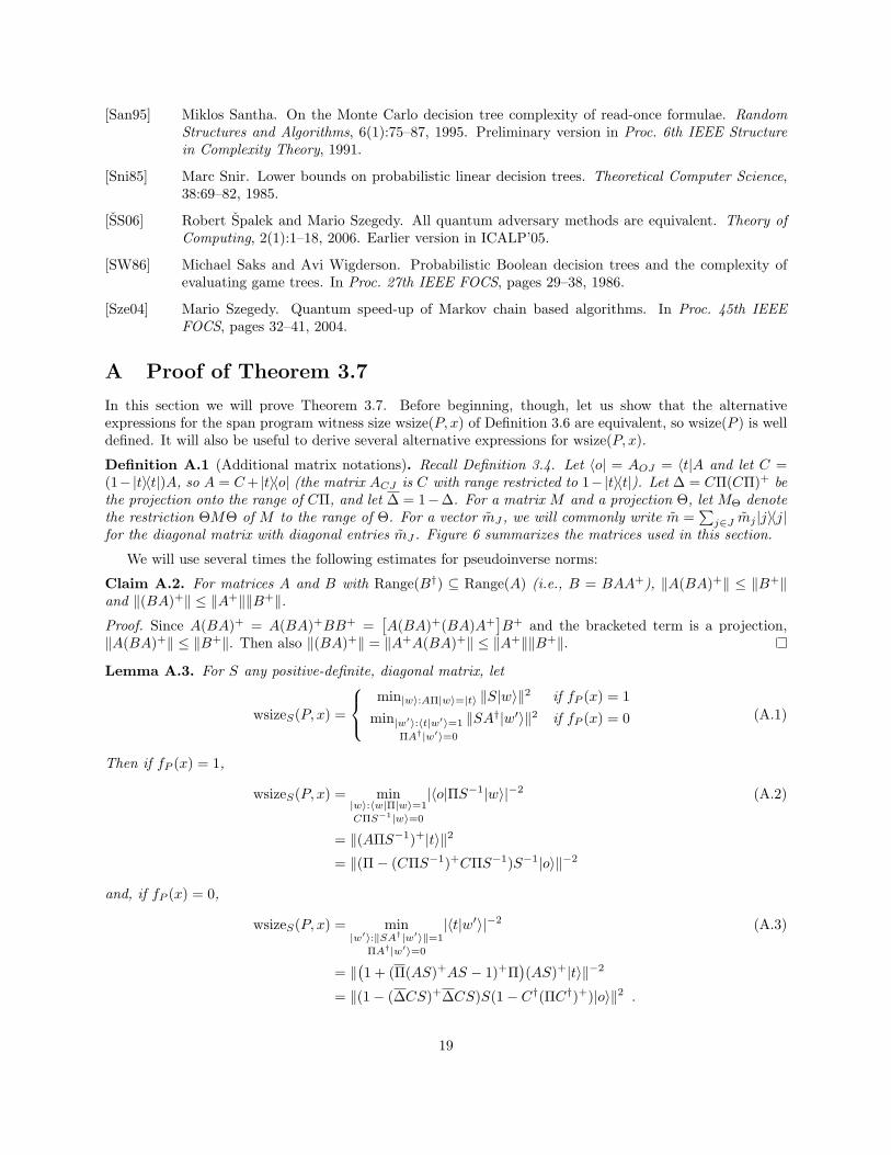
In this section we will prove Theorem 3.7. Before beginning, though, let us show that the alternativeexpressions for the span program witness size wsize(P, x) of Definition 3.6 are equivalent, so wsize(P ) is welldefined. It will also be useful to derive several alternative expressions for wsize(P, x).

Definition A.1 (Additional matrix notations). Recall Definition 3.4. Let 〈o| = AOJ = 〈t|A and let C =(1−|t〉〈t|)A, so A = C+ |t〉〈o| (the matrix ACJ is C with range restricted to 1−|t〉〈t|). Let ∆ = CΠ(CΠ)+ bethe projection onto the range of CΠ, and let ∆ = 1−∆. For a matrix M and a projection Θ, let MΘ denotethe restriction ΘMΘ of M to the range of Θ. For a vector mJ , we will commonly write m =

∑j∈J mj |j〉〈j|

for the diagonal matrix with diagonal entries mJ . Figure 6 summarizes the matrices used in this section.

We will use several times the following estimates for pseudoinverse norms:

Claim A.2. For matrices A and B with Range(B†) ⊆ Range(A) (i.e., B = BAA+), ‖A(BA)+‖ ≤ ‖B+‖and ‖(BA)+‖ ≤ ‖A+‖‖B+‖.Proof. Since A(BA)+ = A(BA)+BB+ =

[A(BA)+(BA)A+

]B+ and the bracketed term is a projection,

‖A(BA)+‖ ≤ ‖B+‖. Then also ‖(BA)+‖ = ‖A+A(BA)+‖ ≤ ‖A+‖‖B+‖.

Lemma A.3. For S any positive-definite, diagonal matrix, let

wsizeS(P, x) =

min|w〉:AΠ|w〉=|t〉 ‖S|w〉‖2 if fP (x) = 1

min|w′〉:〈t|w′〉=1

ΠA†|w′〉=0

‖SA†|w′〉‖2 if fP (x) = 0 (A.1)

Then if fP (x) = 1,

wsizeS(P, x) = min|w〉:〈w|Π|w〉=1

CΠS−1|w〉=0

|〈o|ΠS−1|w〉|−2 (A.2)

= ‖(AΠS−1)+|t〉‖2

= ‖(Π− (CΠS−1)+CΠS−1)S−1|o〉‖−2

and, if fP (x) = 0,

wsizeS(P, x) = min|w′〉:‖SA†|w′〉‖=1

ΠA†|w′〉=0

|〈t|w′〉|−2 (A.3)

= ‖(1 + (Π(AS)+AS − 1)+Π

)(AS)+|t〉‖−2

= ‖(1− (∆CS)+∆CS)S(1− C†(ΠC†)+)|o〉‖2 .

19

Moreover, |w∗S〉 = arg min|w〉:AΠ|w〉=|t〉‖S|w〉‖2 = S−1(AΠS−1)+|t〉 has norm ‖|w∗S〉‖ = O(1) and

|w′∗S 〉 = arg min|w′〉:〈t|w′〉=1

ΠA†|w′〉=0

‖SA†|w′〉‖2 = |t〉 − (ΠC†)+Π|o〉 − (SC†∆)+S(1− C†(ΠC†)+)|o〉

has norm ‖|w′∗S 〉‖ = O(1).In particular, the two different expressions for wsize(P, x) = wsize√z(P, x) in Definition 3.6 are equiva-

lent, so wsize(P, x) and wsize(P ) are well defined.

Proof. Assume fP (x) = 1. That min|w〉:AΠS−1|w〉=|t〉 ‖|w〉‖2 = min|w〉:〈w|Π|w〉=1

CΠS−1|w〉=0

|〈o|ΠS−1|w〉|−2 is immediate.

In general, arg min|x〉:M |x〉=|b〉‖|x〉‖ = M+|b〉; therefore, min|w〉:AΠS−1|w〉=|t〉 ‖|w〉‖2 = ‖(AΠS−1)+|t〉‖2. Bybasic geometry, arg max|w〉:‖Π|w〉‖=1

CΠS−1|w〉=0

|〈o|ΠS−1|w〉| ∝(1 − (CΠS−1)+(CΠS−1)

)ΠS−1|o〉, i.e., is proportional

to the projection of ΠS−1|o〉 onto the space orthogonal to the range of S−1ΠC†. Eq. (A.2) follows.Next assume fP (x) = 0. That min|w′〉:〈t|w′〉=1

ΠA†|w′〉=0

‖SA†|w′〉‖2 = min|w′〉:‖SA†|w′〉‖=1

ΠA†|w′〉=0

|〈t|w′〉|−2 is immediate.

Now, without loss of generality, |t〉 ∈ Range(A) = Range(AS), since otherwise fP is false on every input.Therefore, 〈t|w′〉 = 〈t|(SA†)+(SA†)|w′〉 = 〈t|(SA†)+|w〉 if |w〉 = SA†|w′〉. We want to find the length-onevector |w〉 that is in the range of SA† and also of Π, and that maximizes |〈t|(SA†)+|w〉|2. The answer isclearly the normalized projection of (AS)+|t〉 onto the intersection Range(SA†) ∩ Range(Π). In general,given two projections Π1 and Π2, the projection onto the intersection of their ranges can be written 1 −(Π1Π2 − 1)+(Π1Π2 − 1). Substituting Π1 = Π and Π2 = (AS)+AS gives the second claimed expression.

Finally, we show that min|w′〉:〈t|w′〉=1

ΠA†|w′〉=0

‖SA†|w′〉‖2 = ‖(1 − (∆CS)+∆CS)S(1 − C†(ΠC†)+)|o〉‖2. Since

fP (x) is false, |t〉 does not lie in the span of the true grouped input vectors, |t〉 /∈ Range(AΠ), or equivalentlyΠ|o〉 ∈ Range(ΠC†). Therefore, there exists a vector |w′〉 = |t〉+ |bC〉 that is orthogonal to the span of thetrue columns of A and has inner product one with |t〉. Any such |bC〉 has the form

|bC〉 = −(ΠC†)+Π|o〉+ ∆|v〉 ,

where |v〉 is an arbitrary vector with 〈t|v〉 = 0. We want to choose |v〉 to minimize the squared length of

ΠSA†|w′〉 = SΠ(|o〉+ C†|bC〉)= S(1− C†(ΠC†)+)|o〉+ SC†∆|v〉 . (A.4)

The answer is clearly the squared length of S(1−C†(ΠC†)+)|o〉 projected orthogonal to the range of SC†∆,as claimed. This corresponds to setting |v〉 = −(SC†∆)+S(1− C†(ΠC†)+)|o〉.

The norms of |w∗S〉 and |w′∗S 〉 are bounded using Claim A.2.

Remark A.4. The expressions for witness size in Eqs. (A.2) and (A.3) look quite different depending onwhether fP (x) = 1 or fP (x) = 0, with the latter case being more complicated. It can be seen, though, that|wsize(P, x)−wsize(P †, x)| = O(1) for any fixed span program P , where P † is the dual span program describedin Section 2.3 with fP †(x) = ¬fP (x).

Let us now show that if z′j . zj for all j ∈ J , then wsize√z′(P, x) . wsize(P, x) (Lemma A.6). This willbe useful in showing that wsize(P, x) is a rough upper bound on the exact expressions that we will derive inthe sections below.

Remark A.5. From Definition 3.6, it is immediate that wsize(P, x) is monotone increasing in each inputcomplexity zi.

Lemma A.6. Let S and T be any positive-definite diagonal matrices. Then

wsizeS√1+T (P, x) ≤ wsizeS(P, x) · (1 + ‖T‖) , (A.5)

wsize√S2+T 2(P, x) ≤ wsizeS(P, x) +O(‖T‖2) . (A.6)

In particular, if z′J is such that z′j . zj for all j ∈ J , then wsize√z′(P, x) . wsize√z(P, x) = wsize(P, x).

20

A =∑j |vj〉〈j| = C + |t〉〈o| span program matrix

C = (1− |t〉〈t|)A “constraint” part of the span program〈o| = AOJ = 〈t|A “output” row of the span programΠ =

∑true j |j〉〈j| projection onto true grouped inputs

Π = 1−Π projection onto false grouped inputs

σ =∑j σj |j〉〈j| grouped input squared supports at λ = 0

r =∑i ri|i〉〈i| input ratios ri = aj(i)/bi

r = (AIJ †r−1AIJ − λ)−1 =∑j rj |j〉〈j| grouped input ratios

s = − 1λΠr−1 + 1

λΠr =∑j sj |j〉〈j| grouped input ratio multipliers

z =∑j zj |j〉〈j| grouped input complexities, 1

σj, sj . zj

y = Cs−1/2Π, Y = yy† true constraints scaled down by√s

y = Cs1/2Π, Y = yy† false constraints scaled up by√s

∆ = yy+ = CΠ(CΠ)+ projection onto the range of true constraints∆ = 1−∆ complementary projectionX = −λ2(1 + 1

λCrC†) = Y − λ2(Y + 1) matrix to be inverted

(X/X∆) = X∆ −∆X(X∆)−1X∆ Schur complement of X∆ in X

V = −λ2y†∆X−1∆y = −λ2y†(X/X∆)−1y a part of the inverse of X

V = y†∆(Y∆ + 1)−1∆y a useful O(1) matrix, V − V = O(λ2‖z‖2)

Figure 6: Matrices used in the proof of Theorem 3.7.

Proof. Eq. (A.5) is immediate from the definition in Eq. (A.1). To derive Eq. (A.6), first note that‖√S2 + T 2|v〉‖2 = ‖S|v〉‖2 + ‖T |v〉‖2. Then when fP (x) = 1,

min|w〉:AΠ|w〉=|t〉

(‖S|w〉‖2 + ‖T |w〉‖2) ≤ ‖S|w∗S〉‖2 + ‖T |w∗S〉‖2

= wsizeS(P, x) +O(‖T‖2) ,

where we have used that |w∗S〉 = arg min|w〉:AΠ|w〉=|t〉‖S|w〉‖2 has norm ‖|w∗S〉‖ = O(1) by Lemma A.3. Theargument when fP (x) = 0 is similar:

min|w′〉:〈t|w′〉=1

ΠA†|w′〉=0

(‖SA†|w′〉‖2 + ‖TA†|w′〉‖2) ≤ wsizeS(P, x) + ‖TA†|w′∗S 〉‖2 ,

where |w′∗S 〉 = arg min|w′〉:〈t|w′〉=1

ΠA†|w′〉=0

‖SA†|w′〉‖2 has O(1) norm by Lemma A.3.

A.1 Quantitative eigenvalue-zero spectral analysis of AGP

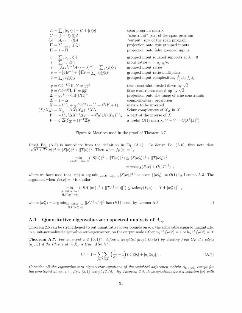
Theorem 2.5 can be strengthened to put quantitative lower bounds on σO, the achievable squared magnitude,in a unit-normalized eigenvalue-zero eigenvector, on the output node either aO if fP (x) = 1 or bO if fP (x) = 0:

Theorem A.7. For an input x ∈ 0, 1n, define a weighted graph GP (x) by deleting from GP the edges(aj , bi) if the ith literal in Xj is true. Also let

W = 1 +∑j∈J

∑i∈Ij

( 1σi− 1)

(|bi〉〈bi|+ |aj〉〈aj |) . (A.7)

Consider all the eigenvalue-zero eigenvector equations of the weighted adjacency matrix AGP (x), except forthe constraint at aO, i.e., Eqs. (2.1) except (2.1d). By Theorem 2.5, these equations have a solution |ψ〉 with

21

〈aO|ψ〉 6= 0 if and only if fP (x) = 1, and have a solution |ψ〉 with 〈bO|ψ〉 6= 0 if and only if fP (x) = 0. Infact, the solution |ψ〉 can be chosen so that the normalized square overlap

σO ≡|(〈aO|+ 〈bO|)|ψ〉|2

〈ψ|W |ψ〉≥ 1

wsize(P, x) + constant, (A.8)

where the constant may depend on P but is independent of the σI , and wsize(P, x) is as defined in Defini-tion 3.6, with 1/σi ≤ zi for all i.

Remark A.8. Note that Theorem A.7 implies the λ = 0 portion of Theorem 3.7. The weights in W meanthat, e.g., setting bi = 1 adds 〈bi|W |bi〉 = 1/σi to the squared normalization factor.

Proof of Theorem A.7. Recall Figure 2. The vertex aj is a shared output node of all the inputs i ∈ Ij . Asin the proof of Theorem 2.5, Eq. (2.1c) implies that aj can be nonzero only if grouped input j is true, i.e.,if all i ∈ Ij evaluate to true.

For j ∈ J , define σj by

σj =

(

1 +∑i∈Ij

(1σi− 1))−1

if j is true∑false i ∈ Ij σi if j is false

(A.9)

From Definition 3.1, 1/σj ≤ zj . Roughly speaking, for each j, the vertices bi for i ∈ Ij can be treated as justa single input vertex with associated weight σj in W . Precisely, if j is true, then 〈aj |W |aj〉 = 1/σj .And if j is false, then the bIj coefficients appear in Eq. (2.1e) only in the quantity 〈j|AIJ(x)†|bIj 〉 =∑

false i ∈ Ij bi. In order to minimize the weighted squared norm 〈bIj |W |bIj 〉 =∑i∈Ij |bi|

2/σi for any fixedvalue of 〈j|AIJ(x)†|bIj 〉, each bi for i false should be set proportional to σi (by Cauchy-Schwarz), so

min|bIj 〉:〈j|AIJ (x)†|bIj 〉=1

〈bIj |W |bIj 〉 =1σj

. (A.10)

Let σ =∑j σj |j〉〈j|.

Case fP (x) = 1: When fP (x) = 1, set aj = 0 for all false grouped inputs j. Set the other aj so asto maximize the magnitude of −aO = AOJ |aJ〉 = 〈o|Π|aJ〉, such that C|aJ〉 = CΠ|aJ〉 = 0 and〈aJ |W |aJ〉 = 〈aJ |Πσ−1|aJ〉 = 1 (Eqs. (2.1b) and (2.1a) at λ = 0). Now, changing variables to|w〉 = σ−1/2|aJ〉,

|aO|2 = max|w〉:〈w|Π|w〉=1

CΠσ1/2|w〉=0

|〈o|Πσ1/2|w〉|2

= 1/wsizeσ−1/2(P, x)≥ 1/wsize(P, x) ,

(A.11)

using Eq. (A.2), 1/σj ≤ zj and the monotonicity of wsize(P, x) (Remark A.5). Finally, dividing by(1 + |aO|2) so that the total norm is one, gives

σO =|aO|2

1 + |aO|2≥ 1

wsize(P, x) + 1. (A.12)

Case fP (x) = 0: When fP (x) = 0, for each true grouped input j set bi = 0 for i ∈ Ij . For each falsej, set bi = 0 for true i ∈ Ij and set bi = fjσi/

∑false i′ ∈ Ij σi′ . Choose |f〉 to maximize |bO|2 such

that 〈f |Πσ−1|f〉 = 1 and, by Eq. (2.1e) at λ = 0, |o〉bO + C†|bC〉 + Π|f〉 = 0. Equivalently, writing

22

|w′〉 =(bObC

)so bO = 〈t|w′〉, we are constrained that Π|f〉 = −A†|w′〉, i.e.,

|bO|2 = max|w′〉:‖σ−1/2A†|w′〉‖=1

ΠA†|w′〉=0

|〈t|w′〉|2

= 1/wsizeσ−1/2(P, x)≥ 1/wsize(P, x)

(A.13)

by Eq. (A.3) and the monotonicity of wsize(P, x). The constructed state has weighted squared norm〈ψ|W |ψ〉 = 1 + ‖|w′∗〉‖2, where |w′∗〉 = arg max|w′〉:‖σ−1/2A†|w′〉‖=1

ΠA†|w′〉=0

|〈t|w′〉|2. Normalizing,

1σO

=1 + ‖|w′∗〉‖2

|bO|2

≤ wsize(P, x) +‖|w′∗〉‖2

|bO|2.

(A.14)

It remains to show that ‖|w′∗〉/bO‖ = O(1). Indeed, 1〈t|w′∗〉 |w

′∗〉 = arg min|w′〉:〈t|w′〉=1

ΠA†|w′〉=0

‖σ−1/2A†|w′〉‖2 =

|w′∗σ−1/2〉 has O(1) norm by Lemma A.3.

A.2 Small-eigenvalue spectral analysis of AGP

Theorem A.9. For a span program P and input x, given sI with 0 < si ≤ zi for all i ∈ I, let s =∑i si|i〉〈i|

and r =∑i ri|i〉〈i| = − 1

λΠs−1 + λΠs. Assume that 0 < λ ≤ ε/si for a small enough constant ε > 0 to bedetermined and for all i ∈ I. Then the equations

bI = r−1AIJaJ (A.15a)λbO = aO +AOJaJ (A.15b)λbC = ACJaJ (A.15c)

λaJ = AOJ†bO +ACJ

†bC +AIJ(x)†bI (A.15d)

have a solution with aO, bO 6= 0. Moreover, if rO = aO/bO and sO is defined as −1/(λrO) or rO/λ if fP (x)is true or false, respectively, then

0 < sO . wsize√z(P, x) , (A.16)

where the grouped input complexities zJ are defined in terms of zI in Definition 3.2.

Proof. Similarly to the argument in Appendix A.1, it will be useful to define a “grouped input ratio” rj sothat, roughly speaking, the vertices bi for i ∈ Ij can be treated as just a single input vertex.

Definition A.10 (Grouped input ratios). For j ∈ J , let rj = (−λ+∑i∈Ij r

−1i )−1, and let r =

∑j rj |j〉〈j| =

(AIJ †r−1AIJ − λ)−1. Like an input ratio ri, rj is large and negative if j is true, and small and positiveif j is false. Therefore let sj = −1/(λrj) if j is true, and sj = rj/λ if j is false. Let s =

∑j sj |j〉〈j| =

− 1λΠr−1 + 1

λΠr, so r = − 1λΠs−1 + λΠs.

Before proceeding, we need to establish that r and s are well defined.

Lemma A.11. Assume that 0 < λ ≤ ε/zi for a small enough constant ε > 0 and for all i ∈ I. Thenr = (AIJ †r−1AIJ − λ)−1 exists, so s exists as well. Moreover, for each grouped input j ∈ J , sj . zj.

23

Proof. By definition,

rj = (−λ+∑i∈Ij

r−1i )−1 =

(− λ− λ

∑true i ∈ Ij

si +1λ

∑false i ∈ Ij

s−1i

)−1

.

If all inputs in Ij are true, then

sj = −1/(λrj) = 1 +∑i∈Ij

si ,

so 1 ≤ sj ≤ 1 +∑i∈Ij zi ≤ 1 + zj .

Now assume at least one input in Ij is false. The true terms can be upper-bounded by λ∑

true i ∈ Ij si ≤λ∑i∈Ij zi ≤ |Ij |ε. On the other hand, if i is false then (λsi)−1 ≥ (λzi)−1 ≥ 1/ε. Therefore, sj > 0, and we

also get sj ≤ zj(1 + ε′λmaxfalse i ∈ Ij zi) for a constant ε′.

Now we will solve for the output ratio rO using Eqs. (A.15b-d). Letting sO = rO/λ in case fP (x) = 0, orsO = −1/(λrO) in case fP (x) = 1, we aim to show that 0 < sO . wsize√s(P, x). This will prove Theorem A.9since, by Lemma A.6, wsize√s(P, x) . wsize√z(P, x) = wsize(P, x). Our proof will follow the sketch belowTheorem 3.7 in Section 3. We start by deriving an exact expression for rO:

Lemma A.12. The solution to Eq. (A.15) has aO = 0 if bO = 0, and otherwise,

rO = λ+ 〈o|(r − 1

λrC†(1 + 1

λCrC†)−1Cr

)|o〉 , (A.17)

provided that r and (1 + 1λCrC

†)−1 exist.

Proof. Recall from Definition A.1 that |o〉 = AOJ† and ACJ is C with range restricted. Substituting

Eqs. (A.15a) and (A.15c) into (A.15d), and rearranging terms gives(λ−AIJ †r−1AIJ −

1λC†C

)|aJ〉 = |o〉bO .

From Eq. (A.15b), if bO 6= 0, then aO/bO = λ− 〈o|aJ〉/bO, so

rO = λ+ 〈o|(r−1 +1λC†C)−1|o〉 (A.18)

= λ+ 〈o|(r − 1

λrC†(1 + 1

λCrC†)−1Cr

)|o〉 ,

by the Woodbury matrix identity [GV96], provided that r and (1 + 1λCrC

†)−1 exist.

Remark A.13 (Form of Eq. (A.17)). Note from Eq. (A.17) that rO is a real number provided that all theinput ratios rI are themselves reals. Also, note that rO depends on C only through C†C (see too Eq. (A.18)in the proof); in particular, left-multiplying C by U where U is any linear isometry (i.e., satisfying U†U = 1)has no effect. Since the grouped input vectors vJ can be arbitrary in Definition 2.1, C†C is in general anarbitrary |J | × |J | positive semidefinite matrix.

Now the main step in simplifying Eq. (A.17) is dividing the matrix we want to invert into a 2× 2 blockmatrix and applying the following well-known claim:

Claim A.14. Let X be an operator, and let ∆ and ∆ = 1−∆ be a projection and its complement. Assumethat X∆ is invertible. Let the “Schur complement” of X be (X/X∆) ≡ X∆ −∆X(X∆)−1X∆. If the Schurcomplement of X is invertible on ∆, then X is invertible, and X−1 is given by:

∆X−1∆ = (X∆)−1 + (X∆)−1X(X/X∆)−1X(X∆)−1 ∆X−1∆ = −(X∆)−1X(X/X∆)−1

∆X−1∆ = −(X/X∆)−1X(X∆)−1 ∆X−1∆ = (X/X∆)−1 (A.19)

24

Proof. Multiply out the matrices.

Lemma A.15. The inverse (1+ 1λCrC

†)−1 exists, provided 0 < λ ≤ ε/zi for a small enough positive constantε and for all i ∈ I.

Proof. Let y = Cs−1/2Π, y = Cs1/2Π, Y = yy† and Y = yy†. We aim to show that X−1 exists, where

X = −λ2(1 +

1λCrC†

)= Y − λ2(Y + 1) .

(A.20)

Let ∆ = yy+ be the projection onto the range of y, and let ∆ = 1−∆. Then

X∆ = Y − λ2∆(Y + 1)∆ ∆X∆ = −λ2∆Y∆

∆X∆ = −λ2∆Y∆ X∆ = −λ2∆(Y + 1)∆ (A.21)

Now since Y is invertible on ∆ (i.e., ∆ = Y Y +), so is X. By the Neumann series,

(X∆)−1 = Y +(1 +O(λ2‖s‖2)) , (A.22)

where we have used that ‖Y ‖ = O(‖s‖) and ‖Y +‖ = O(‖s‖) (Claim A.2), and where we write O(λ2‖s‖2) tomean some matrix with norm so-bounded. In particular, (X∆)−1 is positive definite on ∆.

Let (X/X∆) be the Schur complement of X∆ in X,

(X/X∆) ≡ X∆ −∆X(X∆)−1X∆

= −λ2∆(Y + 1)∆− λ4∆Y (X∆)−1Y∆ . (A.23)

As −(X/X∆) on ∆ is the sum of the positive definite matrix λ2∆ and positive semidefinite matrices, (X/X∆)is negative definite on ∆ and in particular is invertible on ∆.

Since X∆ and (X/X∆) are each invertible, on ∆ and on ∆, respectively, X−1 exists by Claim A.14, asclaimed.

The following discussion will use the notation from the proof of Lemma A.15. It will also be convenientto let S =

√s. We have from Eq. (A.17)

rO = λ+ 〈o|r|o〉+ λ〈o|rC†X−1Cr|o〉 (A.24)

= λ− 1λ〈o|S−2Π|o〉+ λ〈o|S2Π|o〉+

( 1λ〈o|S−1y†X−1yS−1|o〉 +λ3〈o|Sy†X−1yS|o〉−λ(〈o|S−1y†X−1yS|o〉 +〈o|Sy†X−1yS−1|o〉

))

.

Our goal now is to expand the above expression as a series in λ, evaluating the coefficients of 1/λ and of λ,and bounding higher-order terms. In order to expand X−1 as a series, we use the block decomposition of Xand Claim A.14.

Let us start by evaluating two expressions, (X∆)−1 and V = −λ2y†(X/X∆)−1y, that will reappear

frequently in the following analysis.

Claim A.16. (X∆)−1 satisfies

(X∆)−1 = Y + + λ2Y +(Y + 1)Y + + Y +O(λ4‖s‖3)Y + (A.25)

= Y +(1 +O(λ2‖s‖2)) = O(‖s‖) .

Proof. We know that ‖(X∆)−1‖ = O(‖s‖). Note that for matrices A and B, (A + B)−1 = (1 − (A +B)−1B)A−1 = A−1(1 − B(A + B)−1) = A−1 − A−1BA−1 + A−1B(A + B)−1BA−1 provided A and A + Bare invertible. Applying this with A = Y and B = −λ2∆(Y + 1)∆ gives

(X∆)−1 = Y + + λ2Y +(Y + 1)Y + + λ4Y +(Y + 1)(X∆)−1(Y + 1)Y +

= Y + + λ2Y +(Y + 1)Y + + Y +O(λ4‖s‖3)Y + .

25

Claim A.17. Let V = −λ2y†∆X−1∆y = −λ2y†(X/X∆)−1y. Then

V = V +O(λ2‖s‖2) where V = y†∆(Y∆ + 1)−1∆y . (A.26)

In particular, ‖V ‖ < 1 and ‖V ‖ < 1 +O(λ2‖s‖2) = O(1).

Proof. We compute

V = −λ2y†(X∆ −∆X(X∆)−1X∆)−1y

= y†[∆(Y + 1)∆ + λ2∆Y (X∆)−1Y∆

]−1y

= M†[M(1 + λ2y†(X∆)−1y

)M† + 1

]−1M , (A.27)

where M = ∆y. Now λ2y†(X∆)−1y = O(λ2‖s‖2) since y = O(‖√s‖). Therefore, M

(1+λ2y†(X∆)−1y

)M†+1

is the sum of positive-definite and positive-semidefinite matrices, hence is invertible. Again use (A+B)−1 =(1− (A+B)−1B)A−1, now with A = MM† + 1 = Y∆ + 1 and B = λ2My†(X∆)−1yM†, to get

V = V − V (λ2y†(X∆)−1y)V

= V ·[1 + (λ2y†(X∆)−1y)V

]−1

, (A.28)

provided the inverse right-multiplying V exists. Indeed, M†(MM† + 1)−1M < 1 for an arbitrary matrixM and in particular for M = ∆y (if the singular-value decomposition of M is M =

∑imi|i〉〈i′|, then

M†(MM† + 1)−1M =∑i

m2i

m2i+1|i′〉〈i′|). Therefore the inverse does exist, and we obtain Eq. (A.26).

Now, using Claim A.16 and Claim A.17, we find

∆X−1∆ = (X∆)−1 + (X∆)−1X(X/X∆)−1X(X∆)−1

= (X∆)−1 − λ2(X∆)−1yV y†(X∆)−1

= Y + + λ2Y +(Y + 1)Y + + Y +O(λ4‖s‖3)Y +

− λ2Y +(1 +O(λ2‖s‖2))y(V +O(λ2‖s‖2)

)y†(1 +O(λ2‖s‖2))Y +

= Y + + λ2Y +(−yV y† + Y + 1 +O(λ2‖s‖3)

)Y + , (A.29)

and

∆X−1∆y = λ2(X∆)−1Y (X/X∆)−1y

= −(X∆)−1yV

= −Y +(1 +O(λ2‖s‖2))y(V +O(λ2‖s‖2))

= −Y +yV + Y + ·O(λ2‖s‖5/2) . (A.30)

In particular, ‖∆X−1∆‖ = O(‖s‖) and ‖∆X−1∆y‖ = O(‖s‖3/2).Let us now substitute the expressions we have derived into Eq. (A.24) for rO. Consider each of the terms

involving X−1 separately. First of all,

1λ〈o|S−1y†X−1yS−1|o〉 =

1λ〈o|S−1y†(∆X−1∆)yS−1|o〉

=1λ〈o|ΠS−1y+yS−1Π|o〉 (A.31)

+ λ〈o|ΠS−1y+(1 + Y − yV y†

)(y†)+S−1Π|o〉

+O(λ3‖s‖3) ,

26

where we have substituted Eq. (A.29) and applied ‖S−1y†Y +‖ = ‖S−1y+‖ = O(1) (Claim A.2).Also, by Claim A.17 and Eqs. (A.29), (A.30),

λ3〈o|Sy†X−1yS|o〉 = λ3〈o|Sy†(∆ + ∆)X−1(∆ + ∆)yS|o〉= −λ〈o|SV S|o〉+O(λ3‖s‖3) (A.32)

= −λ〈o|ΠSV SΠ|o〉+O(λ3‖s‖3) .

Lastly, by Eqs. (A.29), (A.30),

λ〈o|S−1y†X−1yS|o〉 = λ〈o|S−1y†∆X−1(∆ + ∆)yS|o〉= λ〈o|S−1y†Y +(1 +O(λ2‖s‖2))yS|o〉

− λ〈o|S−1y†Y +[yV +O(λ2‖s‖5/2)

]S|o〉

= λ〈o|ΠS−1y+(y − yV )SΠ|o〉+O(λ3‖s‖3) . (A.33)

Substituting Eqs. (A.31), (A.32), (A.33) into the expression for rO gives

rO = − 1λ‖(1− y+y)S−1Π|o〉‖2 + λ〈v|

(1− V

)|v〉+O(λ+ λ3‖s‖3) , (A.34)

where |v〉 = (SΠ− y†(y†)+S−1)|o〉. From the singular-value decomposition, one infers that (1−M†(MM†+1)−1M)− (1−M+M) = M+(1− (MM† + 1)−1)(M†)+ for any matrix M , and in particular for M = ∆y.Moreover, 〈v|(∆y)

+(1 − (Y∆ + 1)−1)((∆y)

†)+|v〉 = O(1), since ‖S(∆y)

+‖ = O(1) and ‖〈v|S−1‖ = O(1).Therefore the above equation simplifies to

rO = − 1λ‖(1− y+y)S−1Π|o〉‖2 + λ

(‖(1− (∆y)

+(∆y))|v〉‖2 +O(1)

)+O(λ3‖s‖3) . (A.35)

This is as far as we can simplify rO in general. When fP (x) = 1, the first term is −1/(λwsizeS(P, x)),as desired, using the last expression of Eq. (A.2) for wsizeS(P, x). Assume then that fP (x) = 0, i.e.,Π|o〉 ∈ Range(ΠC†). In this case, the first term in Eq. (A.35) is zero, and the second term can be simplifiedslightly further. Using (y†)+S−1|o〉 = (ΠS−1C†)+S−1Π|o〉 = (ΠC†)+|o〉 and ΠC†(ΠC†)+|o〉 = Π|o〉,

|v〉 = (SΠ− y†(ΠC†)+)|o〉= (SΠ− y†(ΠC†)+)|o〉+ SΠ(1− C†(ΠC†)+)|o〉= S(1− C†(ΠC†)+)|o〉 .

(A.36)

Moreover, since ∆CSΠ = 0, ∆y = ∆CSΠ = ∆CS. Therefore, ‖(1 − (∆y)+

(∆y))|v〉‖2 = wsizeS(P, x), asdesired, using the last expression of Eq. (A.3) for wsizeS(P, x). This concludes the proof of Theorem A.9.

Theorem A.9 completes the λ 6= 0 portion of Theorem 3.7, finishing its proof.

B Quantum algorithm

The approach outlined in Section 4.4 is slightly indirect. To motivate it, we begin by briefly consideringin Section B.1 a more direct algorithm ALG′, that runs phase estimation directly on exp(iAGP (x)). ALG

′

is analogous to the algorithm described by Cleve et al. [CCJY07] soon after the original NAND formulaevaluation paper [FGG07]. Algorithm ALG′ is nearly optimal, but not quite. The operator exp(iAGP (x)) isa continuous-time quantum walk, and the overhead can be thought of as coming from simulating continuous-time quantum dynamics with a discrete computational model, in particular with discrete oracle queries. Toavoid this overhead, the proof of Theorem 4.7 in Section B.2 works with a discrete-time quantum walk.

The approach in Section B.1 is optional motivation, and the reader may choose to skip directly toSection B.2.

27

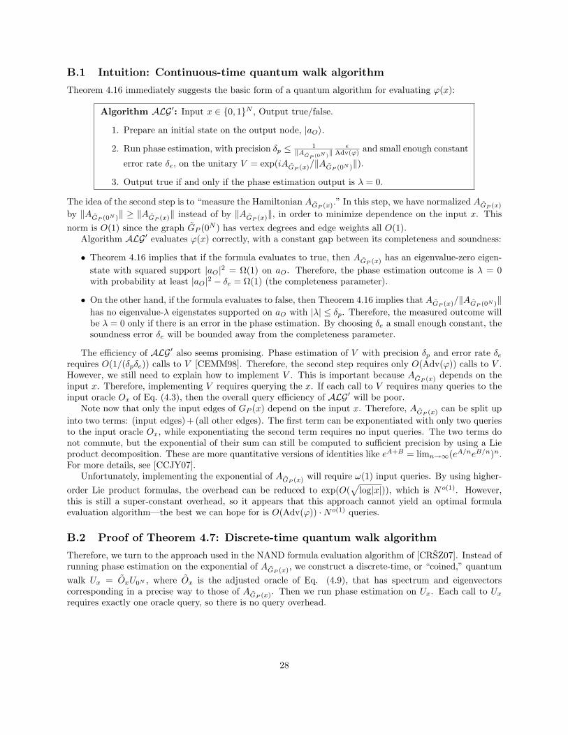
B.1 Intuition: Continuous-time quantum walk algorithm

Theorem 4.16 immediately suggests the basic form of a quantum algorithm for evaluating ϕ(x):

Algorithm ALG′: Input x ∈ 0, 1N , Output true/false.

1. Prepare an initial state on the output node, |aO〉.

2. Run phase estimation, with precision δp ≤ 1‖AGP (0N )‖

εAdv(ϕ) and small enough constant

error rate δe, on the unitary V = exp(iAGP (x)/‖AGP (0N )‖).

3. Output true if and only if the phase estimation output is λ = 0.

The idea of the second step is to “measure the Hamiltonian AGP (x).” In this step, we have normalized AGP (x)

by ‖AGP (0N )‖ ≥ ‖AGP (x)‖ instead of by ‖AGP (x)‖, in order to minimize dependence on the input x. Thisnorm is O(1) since the graph GP (0N ) has vertex degrees and edge weights all O(1).

Algorithm ALG′ evaluates ϕ(x) correctly, with a constant gap between its completeness and soundness:

• Theorem 4.16 implies that if the formula evaluates to true, then AGP (x) has an eigenvalue-zero eigen-state with squared support |aO|2 = Ω(1) on aO. Therefore, the phase estimation outcome is λ = 0with probability at least |aO|2 − δe = Ω(1) (the completeness parameter).

• On the other hand, if the formula evaluates to false, then Theorem 4.16 implies that AGP (x)/‖AGP (0N )‖has no eigenvalue-λ eigenstates supported on aO with |λ| ≤ δp. Therefore, the measured outcome willbe λ = 0 only if there is an error in the phase estimation. By choosing δe a small enough constant, thesoundness error δe will be bounded away from the completeness parameter.

The efficiency of ALG′ also seems promising. Phase estimation of V with precision δp and error rate δerequires O(1/(δpδe)) calls to V [CEMM98]. Therefore, the second step requires only O(Adv(ϕ)) calls to V .However, we still need to explain how to implement V . This is important because AGP (x) depends on theinput x. Therefore, implementing V requires querying the x. If each call to V requires many queries to theinput oracle Ox of Eq. (4.3), then the overall query efficiency of ALG′ will be poor.

Note now that only the input edges of GP (x) depend on the input x. Therefore, AGP (x) can be split upinto two terms: (input edges) + (all other edges). The first term can be exponentiated with only two queriesto the input oracle Ox, while exponentiating the second term requires no input queries. The two terms donot commute, but the exponential of their sum can still be computed to sufficient precision by using a Lieproduct decomposition. These are more quantitative versions of identities like eA+B = limn→∞(eA/neB/n)n.For more details, see [CCJY07].

Unfortunately, implementing the exponential of AGP (x) will require ω(1) input queries. By using higher-order Lie product formulas, the overhead can be reduced to exp(O(

√log|x|)), which is No(1). However,

this is still a super-constant overhead, so it appears that this approach cannot yield an optimal formulaevaluation algorithm—the best we can hope for is O(Adv(ϕ)) ·No(1) queries.

B.2 Proof of Theorem 4.7: Discrete-time quantum walk algorithm

Therefore, we turn to the approach used in the NAND formula evaluation algorithm of [CRSZ07]. Instead ofrunning phase estimation on the exponential of AGP (x), we construct a discrete-time, or “coined,” quantumwalk Ux = OxU0N , where Ox is the adjusted oracle of Eq. (4.9), that has spectrum and eigenvectorscorresponding in a precise way to those of AGP (x). Then we run phase estimation on Ux. Each call to Uxrequires exactly one oracle query, so there is no query overhead.

28

B.2.1 Construction of the coined quantum walk Ux

The first step in constructing Ux is to decompose AGP (0N ) into (constant)·∆†∆, where ∆ is a square matrixwith row norms one, and denotes the entrywise matrix product. We follow [CRSZ07]. One minor technicaldifference, though, is that for us, AGP (x) is a Hermitian matrix with possibly complex entries. In [CRSZ07],the analogous weighted adjacency matrix, for the NAND formula ϕ, is a real symmetric matrix. Therefore,we need to slightly modify the construction of ∆ to obtain the correct phases for the entries of AGP (0N ).

Definition B.1. For notational convenience, let A = AGP (0N ) be the weighted adjacency matrix for GP (0N ).(Recall from Theorem 4.16 that GP (0N ) is the same as GP except with the edge weight on the output edge(aO, bO) reduced.) A =

∑v,w Av,w|v〉〈w| is a Hermitian matrix.

GP (0N ) is a bipartite graph, so we may color each vertex red or black, such that every edge is betweenone red vertex and one black vertex.

Claim B.2. Let A′ =∑v,w|Av,w||v〉〈w| be the entrywise absolute value of A. A′ is a real symmetric

matrix. Let ‖A′‖ be the largest-magnitude eigenvalue of A′. Let |δ〉 be the principle eigenvector of A′, with〈v|δ〉 = δv > 0 for every v, and let

∆ =1√‖A′‖

∑black vred w

((√Av,w

)∗√δwδv|v〉〈w|+

√Av,w

√δvδw|w〉〈v|

). (B.1)

Then ∆ has all row norms one, and A = ‖A′‖ ·∆† ∆.

Proof. Since A′ has nonnegative entries, the principal eigenvector |δ〉 is also nonnegative. Since GP (0N ) isa connected graph, δv > 0 for every v. Hence ∆ is well defined up to choice of sign of the square root, whichdoesn’t matter.

By construction, for all v and w, ∆∗v,w∆w,v = Av,w/‖A′‖, i.e., ‖A′‖ · ∆† ∆ = A. Furthermore, the

squared norm of the v-th row of ∆ is∑w|∆v,w|2 = 1

‖A′‖1δv

∑w A′v,wδw = 1

‖A′‖(A′δ)vδv

= 1.

Remark B.3. In defining ∆, we have evenly divided the complex phases of entries of A between red-blackand black-red terms. However, any division of the phases would have worked. For example, Claim B.2 wouldalso hold with Eq. (B.1) replaced by ∆ = 1√

‖A′‖

∑black vred w

(A∗v,w√|Av,w|

√δwδv|v〉〈w|+

√|Av,w| δvδw |w〉〈v|

).

We can now apply Szegedy’s correspondence theorem [Sze04] to relate the spectrum of AGP to that of adiscrete-time coined quantum walk unitary.

Theorem B.4 ([Sze04]). Let |v〉 : v ∈ V be an orthonormal basis for HV . For each v ∈ V , let |v〉 =|v〉 ⊗

∑w∈V δvw|w〉 ∈ HV ⊗HV , where 〈v|v〉 =

∑w|δvw|2 = 1. Let T =

∑v |v〉〈v| and Π = TT † =

∑v |v〉〈v|

be the projection onto the span of the |v〉s. Let S =∑v,w |v, w〉〈w, v|, a swap. Let U = (2Π − 1)S, a swap

followed by reflection about the span of the |v〉s. Let M = T †ST =∑v,w δ

∗vwδwv|v〉〈w|.

Then the spectral decomposition of U corresponds to that of M as follows: Take |λα〉 a completeset of orthonormal eigenvectors of the Hermitian matrix M with respective eigenvalues λα. Let Rα =SpanT |λα〉, ST |λα〉. Then Ra ⊥ Rα′ for α 6= α′; let R = ⊕αRα. U fixes the spaces Ra and is −S on R⊥.The eigenvalues and eigenvectors of U within Ra are given by βα,± = λα± i

√1− λ2

α and (1 +βα,±S)T |λα〉,respectively.

A proof of Theorem B.4 in the above form is given in [CRSZ07], and see [MNRS07].

Remark B.5 (Coined quantum walks). The operator U = (2Π−1)S in Theorem B.4 is known as a “coinedquantum walk.” S is known as the “step operator,” and the reflection (2Π − 1) is the “coin-flip operator.”On the space R, (2Π− 1) decomposes as

∑v |v〉〈v| ⊗ (reflection about

∑w δvw|w〉).

In a classical random walk on a graph, a coin is flipped between each step to decide which adjacent vertexto step to next. In a coined quantum walk, on the other hand, the coin is maintained as part of the coherentquantum state, and is reflected between steps (also known as “diffusion”).

29

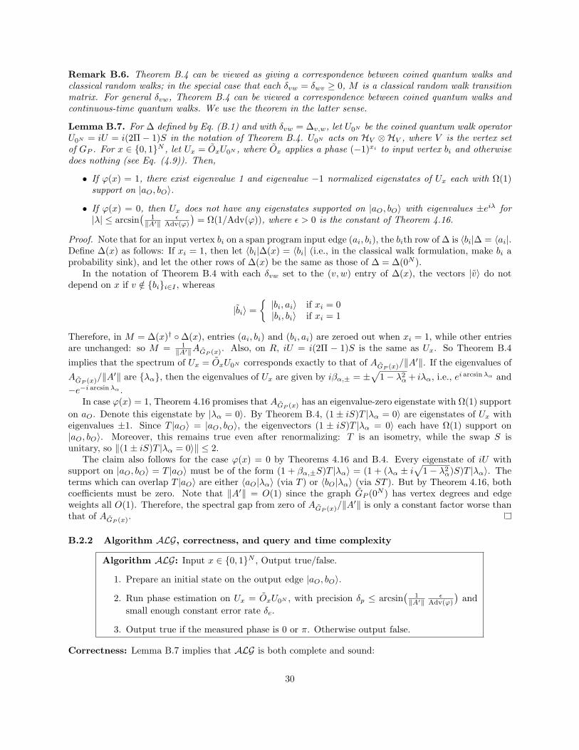
Remark B.6. Theorem B.4 can be viewed as giving a correspondence between coined quantum walks andclassical random walks; in the special case that each δvw = δwv ≥ 0, M is a classical random walk transitionmatrix. For general δvw, Theorem B.4 can be viewed a correspondence between coined quantum walks andcontinuous-time quantum walks. We use the theorem in the latter sense.

Lemma B.7. For ∆ defined by Eq. (B.1) and with δvw = ∆v,w, let U0N be the coined quantum walk operatorU0N = iU = i(2Π− 1)S in the notation of Theorem B.4. U0N acts on HV ⊗HV , where V is the vertex setof GP . For x ∈ 0, 1N , let Ux = OxU0N , where Ox applies a phase (−1)xi to input vertex bi and otherwisedoes nothing (see Eq. (4.9)). Then,

• If ϕ(x) = 1, there exist eigenvalue 1 and eigenvalue −1 normalized eigenstates of Ux each with Ω(1)support on |aO, bO〉.

• If ϕ(x) = 0, then Ux does not have any eigenstates supported on |aO, bO〉 with eigenvalues ±eiλ for|λ| ≤ arcsin

(1‖A′‖

εAdv(ϕ)

)= Ω(1/Adv(ϕ)), where ε > 0 is the constant of Theorem 4.16.

Proof. Note that for an input vertex bi on a span program input edge (ai, bi), the bith row of ∆ is 〈bi|∆ = 〈ai|.Define ∆(x) as follows: If xi = 1, then let 〈bi|∆(x) = 〈bi| (i.e., in the classical walk formulation, make bi aprobability sink), and let the other rows of ∆(x) be the same as those of ∆ = ∆(0N ).

In the notation of Theorem B.4 with each δvw set to the (v, w) entry of ∆(x), the vectors |v〉 do notdepend on x if v /∈ bii∈I , whereas

|bi〉 =|bi, ai〉 if xi = 0|bi, bi〉 if xi = 1

Therefore, in M = ∆(x)† ∆(x), entries (ai, bi) and (bi, ai) are zeroed out when xi = 1, while other entriesare unchanged: so M = 1

‖A′‖AGP (x). Also, on R, iU = i(2Π − 1)S is the same as Ux. So Theorem B.4

implies that the spectrum of Ux = OxU0N corresponds exactly to that of AGP (x)/‖A′‖. If the eigenvalues ofAGP (x)/‖A′‖ are λα, then the eigenvalues of Ux are given by iβα,± = ±

√1− λ2

α + iλα, i.e., ei arcsinλα and−e−i arcsinλα .

In case ϕ(x) = 1, Theorem 4.16 promises that AGP (x) has an eigenvalue-zero eigenstate with Ω(1) supporton aO. Denote this eigenstate by |λα = 0〉. By Theorem B.4, (1± iS)T |λα = 0〉 are eigenstates of Ux witheigenvalues ±1. Since T |aO〉 = |aO, bO〉, the eigenvectors (1 ± iS)T |λα = 0〉 each have Ω(1) support on|aO, bO〉. Moreover, this remains true even after renormalizing: T is an isometry, while the swap S isunitary, so ‖(1± iS)T |λα = 0〉‖ ≤ 2.

The claim also follows for the case ϕ(x) = 0 by Theorems 4.16 and B.4. Every eigenstate of iU withsupport on |aO, bO〉 = T |aO〉 must be of the form (1 + βα,±S)T |λα〉 = (1 + (λα ± i

√1− λ2

α)S)T |λα〉. Theterms which can overlap T |aO〉 are either 〈aO|λα〉 (via T ) or 〈bO|λα〉 (via ST ). But by Theorem 4.16, bothcoefficients must be zero. Note that ‖A′‖ = O(1) since the graph GP (0N ) has vertex degrees and edgeweights all O(1). Therefore, the spectral gap from zero of AGP (x)/‖A′‖ is only a constant factor worse thanthat of AGP (x).

B.2.2 Algorithm ALG, correctness, and query and time complexity

Algorithm ALG: Input x ∈ 0, 1N , Output true/false.

1. Prepare an initial state on the output edge |aO, bO〉.

2. Run phase estimation on Ux = OxU0N , with precision δp ≤ arcsin(

1‖A′‖

εAdv(ϕ)

)and

small enough constant error rate δe.

3. Output true if the measured phase is 0 or π. Otherwise output false.

Correctness: Lemma B.7 implies that ALG is both complete and sound:

30

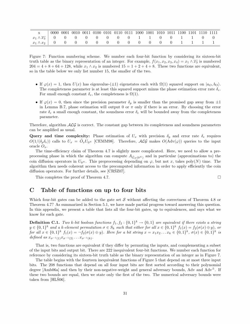
x 0000 0001 0010 0011 0100 0101 0110 0111 1000 1001 1010 1011 1100 1101 1110 1111x1 ∧ x3 0 0 0 0 0 0 0 0 1 1 0 0 1 1 0 0x1 ∧ x2 0 0 0 0 0 0 0 0 0 0 0 0 1 1 1 1

Figure 7: Function numbering scheme. We number each four-bit function by considering its sixteen-bittruth table as the binary representation of an integer. For example, f(x1, x2, x3, x4) = x1 ∧ x3 is numbered204 = 4 + 8 + 64 + 128, while x1 ∧ x2 is numbered 15 = 1 + 2 + 4 + 8. These two functions are equivalent,so in the table below we only list number 15, the smaller of the two.

• If ϕ(x) = 1, then U(x) has eigenvalue-(±1) eigenstates each with Ω(1) squared support on |aO, bO〉.The completeness parameter is at least this squared support minus the phase estimation error rate δe.For small enough constant δe, the completeness is Ω(1).

• If ϕ(x) = 0, then since the precision parameter δp is smaller than the promised gap away from ±1in Lemma B.7, phase estimation will output 0 or π only if there is an error. By choosing the errorrate δe a small enough constant, the soundness error δe will be bounded away from the completenessparameter.

Therefore, algorithm ALG is correct. The constant gap between its completeness and soundness parameterscan be amplified as usual.Query and time complexity: Phase estimation of Ux with precision δp and error rate δe requiresO(1/(δpδe)) calls to Ux = OxU0N [CEMM98]. Therefore, ALG makes O(Adv(ϕ)) queries to the inputoracle Ox.

The time-efficiency claim of Theorem 4.7 is slightly more complicated. Here, we need to allow a pre-processing phase in which the algorithm can compute AGP (0N ) and in particular (approximations to) thecoin diffusion operators in U0N . This preprocessing depending on ϕ, but not x, takes poly(N) time. Thealgorithm then needs coherent access to the precomputed information in order to apply efficiently the coindiffusion operators. For further details, see [CRSZ07].

This completes the proof of Theorem 4.7.

C Table of functions on up to four bits

Which four-bit gates can be added to the gate set S without affecting the correctness of Theorem 4.8 orTheorem 4.7? As summarized in Section 5.1, we have made partial progress toward answering this question.In this appendix, we present a table that lists all the four-bit gates, up to equivalences, and says what weknow for each gate.

Definition C.1. Two k-bit boolean functions f1, f2 : 0, 1k → 0, 1 are equivalent if there exists a stringy ∈ 0, 1k and a k-element permutation σ ∈ Sk such that either for all x ∈ 0, 1k f1(x) = f2(σ(x)⊕ y), orfor all x ∈ 0, 1k f1(x) = ¬f2(σ(x) ⊕ y). Here for a bit string x = x1x2 . . . xk ∈ 0, 1k, σ(x) ∈ 0, 1k isdefined as xσ−1(1)xσ−1(2) . . . xσ−1(k).

That is, two functions are equivalent if they differ by permuting the inputs, and complementing a subsetof the input bits and output bit. There are 222 inequivalent four-bit functions. We number each function forreference by considering its sixteen-bit truth table as the binary representation of an integer as in Figure 7.

The table begins with the fourteen inequivalent functions of Figure 5 that depend on at most three inputbits. The 208 functions that depend on all four input bits are first sorted according to their polynomialdegree [Amb06a] and then by their non-negative-weight and general adversary bounds, Adv and Adv±. Ifthese two bounds are equal, then we state only the first of the two. The numerical adversary bounds weretaken from [HLS06].

31

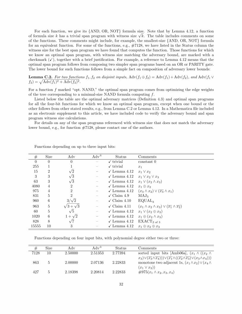
For each function, we give its AND, OR, NOT formula size. Note that by Lemma 4.12, a functionof formula size k has a trivial span program with witness size

√k. The table includes comments on some

of the functions. These comments might include, for example, the smallest-size AND, OR, NOT formulafor an equivalent function. For some of the functions, e.g., #7128, we have listed in the Status column thewitness size for the best span program we have found that computes the function. Those functions for whichwe know an optimal span program, with witness size matching the adversary bound, are marked with acheckmark (X), together with a brief justification. For example, a reference to Lemma 4.12 means that theoptimal span program follows from composing two simpler span programs based on an OR or PARITY gate.The lower bound for such functions follows from a simple fact on composition of adversary lower bounds:

Lemma C.2. For two functions f1, f2 on disjoint inputs, Adv(f1⊕f2) = Adv(f1) +Adv(f2), and Adv(f1∨f2) =

√Adv(f1)2 + Adv(f2)2.

For a function f marked “opt. NAND,” the optimal span program comes from optimizing the edge weightsof the tree corresponding to a minimal-size NAND formula computing f .

Listed below the table are the optimal adversary matrices (Definition 4.3) and optimal span programsfor all the four-bit functions for which we know an optimal span program, except when one bound or theother follows from other stated results, e.g., from Lemma C.2 or Lemma 4.12. In a Mathematica file includedas an electronic supplement to this article, we have included code to verify the adversary bound and spanprogram witness size calculations.

For details on any of the span programs referenced with witness size that does not match the adversarylower bound, e.g., for function #7128, please contact one of the authors.

Functions depending on up to three input bits:

# Size Adv Adv± Status Comments0 0 0 – X trivial constant 0

255 1 1 – X trivial x1

15 2√

2 – X Lemma 4.12 x1 ∨ x2

3 3√

3 – X Lemma 4.12 x1 ∨ x2 ∨ x3

63 3√

3 – X Lemma 4.12 x1 ∨ (x2 ∧ x3)4080 4 2 – X Lemma 4.12 x1 ⊕ x2

975 4 2 – X Lemma 4.12 (x3 ∧ x2) ∨ (x3 ∧ x1)831 5 2 – XClaim 4.9 MAJ3

960 6 3/√

2 – XClaim 4.10 EQUAL3

963 5√

3 +√

3 – XClaim 4.11 (x1 ∧ x2 ∧ x3) ∨ (x1 ∧ x2)60 5

√5 – X Lemma 4.12 x1 ∨ (x2 ⊕ x3)

1020 6 1 +√

2 – X Lemma 4.12 x1 ⊕ (x2 ∧ x3)828 8

√7 – X Lemma 4.12 EXACT2 of 3

15555 10 3 – X Lemma 4.12 x1 ⊕ x2 ⊕ x3

Functions depending on four input bits, with polynomial degree either two or three:

# Size Adv Adv± Status Comments7128 10 2.50000 2.51353 2.77394 sorted input bits [Amb06a], (x1 ∧ ((x2 ∧

x3)∨(x3∧x4)))∨(x1∧((x2∧x3)∨(x3∧x4)))863 5 2.00000 2.07136 2.22833 monotone two adjacent 1s, (x1∧x2)∨(x4∧

(x1 ∨ x3))427 5 2.18398 2.20814 2.22833 #975(x1 ∧ x2, x3, x4)

32

# Size Adv Adv± Status Comments27 5

√5 – X Lemma 4.12 x1 ∧#975(x2, x3, x4)

393 6 4/√

3 – X opt. NAND (x1 ∧ x2 ∧ x3) ∨ (x1 ∧ x2 ∧ x4)383 7 2.30278 2.34406

√4 +√

3 (x1 ∧ x2 ∧ x3) ∨ ((x1 ∨ x2 ∨ x3) ∧ x4)126 7

√11/2 – X Lemma 4.12 x1 ∧ ¬EQUAL3(x2, x3, x4)

24 7√

11/2 – X Lemma 4.12 x1 ∧ EQUAL3(x2, x3, x4)303 6 2.35829 – 1 +

√2 ((x1 ∨ x2) ∧ x3) ∨ ((x1 ∨ x2) ∧ x4), span

program size 5495 6 1 +

√2 – X opt. NAND #975(x1, x2, x3 ∧ x4)

989 6 1 +√

2 – X opt. gadget (x1 ∧ x2 ∧ x3) ∨ (x1 ∧ (x2 ∨ x4))965 7 2.41531 2.42653 2.59234 (x1 ∧ x2 ∧ x3) ∨ (x4 ∧ x3) ∨ (x4 ∧ x2)987 7 2.43128 2.44711424 8

√6 – X opt. NAND EQUAL3(x1, x2, x3 ∧ x4)

2034 7 2.47323 2.48653429 7 2.48837 2.50826490 8 2.52207 2.52326281 8 2.51464 2.540192022 8 2.55719 2.581891968 8 2

√5/3 – X opt. NAND (x1 ∧ x2 ∧ (x3 ∨ x4))∨ (x1 ∧ x2 ∧ (x3 ∨ x4))

1782 7 2.56155 2.59040 2.61804 #975(x1 ⊕ x2, x3, x4)984 8 2.58539 2.602821973 8 2.61704 2.635101910 8

√7 – X opt. NAND (x1 ∧ x2 ∧ x3 ∧ x4) ∨ (x1 ∧ x2) ∨ (x3 ∧ x4)

317 8√

7 – X Lemma 4.12 (x1 ∧ x2 ∧ x3) ∨MAJ3(x2, x3, x4)858 8 2.64575 2.64658

√5 + 2

√2 (x1 ∧ x2 ∧ x3)∨ (x3 ∧ x4)∨ (x1 ∧ (x2 ∨ x3))

300 9 2.69932 2.705956030 10 2.70928 – 3 (x1 ∧ (x2 ∨ x3) ∧ (x2 ∨ x4)) ∨ (x1 ∧ (x2 ∨

x3) ∧ (x2 ∨ x4)), classical three-query alg.894 10 2.70808 2.719821714 10 2.75018 2.759441980 9 2.75779 2.774691719 9 2.76916 2.78319366 10 2.76569 2.803416042 10 2.84104 2.849231716 10 2.86854 2.881861680 12 3 – X opt. NAND EQUAL3(x1, x2, x3 ⊕ x4)1695 10 3 – X opt. NAND #975(x1, x2, x3 ⊕ x4), tight classical alg.5790 10 3 – X opt. NAND (x1 ∧ (x2 ∨ x3) ∧ (x2 ∨ x4)) ∨ (x1 ∧ (x2 ∨

x3) ∧ (x2 ∨ x3)), tight classical alg.7140 10 3 – X Lemma 4.12 x1 ⊕#975(x2, x3, x4), tight classical alg.1683 11 3.00283 3.010095766 12 3.02533 3.035956627 12 3.01470 3.049335783 12 3.03917 3.072946375 14 1 +

√9/2 – X Lemma 4.12 x1 ⊕ EQUAL3(x2, x3, x4)

Functions depending on four input bits, with polynomial degree four:

# Size Adv Adv± Status Comments1 4 2 – X Lemma 4.12 x1 ∧ x2 ∧ x3 ∧ x4

33

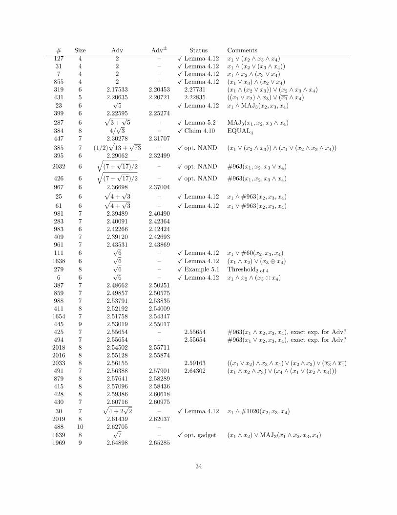
# Size Adv Adv± Status Comments127 4 2 – X Lemma 4.12 x1 ∨ (x2 ∧ x3 ∧ x4)31 4 2 – X Lemma 4.12 x1 ∧ (x2 ∨ (x3 ∧ x4))7 4 2 – X Lemma 4.12 x1 ∧ x2 ∧ (x3 ∨ x4)

855 4 2 – X Lemma 4.12 (x1 ∨ x3) ∧ (x2 ∨ x4)319 6 2.17533 2.20453 2.27731 (x1 ∧ (x2 ∨ x3)) ∨ (x2 ∧ x3 ∧ x4)431 5 2.20635 2.20721 2.22835 ((x1 ∨ x2) ∧ x3) ∨ (x1 ∧ x4)23 6

√5 – X Lemma 4.12 x1 ∧MAJ3(x2, x3, x4)

399 6 2.22595 2.25274287 6

√3 +√

5 – X Lemma 5.2 MAJ3(x1, x2, x3 ∧ x4)384 8 4/

√3 – XClaim 4.10 EQUAL4

447 7 2.30278 2.31707385 7 (1/2)

√13 +

√73 – X opt. NAND (x1 ∨ (x2 ∧ x3)) ∧ (x1 ∨ (x2 ∧ x3 ∧ x4))

395 6 2.29062 2.32499

2032 6√

(7 +√

17)/2 – X opt. NAND #963(x1, x2, x3 ∨ x4)

426 6√

(7 +√

17)/2 – X opt. NAND #963(x1, x2, x3 ∧ x4)967 6 2.36698 2.3700425 6

√4 +√

3 – X Lemma 4.12 x1 ∧#963(x2, x3, x4)61 6

√4 +√

3 – X Lemma 4.12 x1 ∨#963(x2, x3, x4)981 7 2.39489 2.40490283 7 2.40091 2.42364983 6 2.42266 2.42424409 7 2.39120 2.42693961 7 2.43531 2.43869111 6

√6 – X Lemma 4.12 x1 ∨#60(x2, x3, x4)

1638 6√

6 – X Lemma 4.12 (x1 ∧ x2) ∨ (x3 ⊕ x4)279 8

√6 – XExample 5.1 Threshold2 of 4

6 6√

6 – X Lemma 4.12 x1 ∧ x2 ∧ (x3 ⊕ x4)387 7 2.48662 2.50251859 7 2.49857 2.50575988 7 2.53791 2.53835411 8 2.52192 2.540091654 7 2.51758 2.54347445 9 2.53019 2.55017425 7 2.55654 – 2.55654 #963(x1 ∧ x2, x3, x4), exact exp. for Adv?494 7 2.55654 – 2.55654 #963(x1 ∨ x2, x3, x4), exact exp. for Adv?2018 8 2.54502 2.557112016 8 2.55128 2.558742033 8 2.56155 – 2.59163 ((x1 ∨ x2)∧ x3 ∧ x4)∨ (x2 ∧ x3)∨ (x3 ∧ x4)491 7 2.56388 2.57901 2.64302 (x1 ∧ x2 ∧ x3) ∨ (x4 ∧ (x1 ∨ (x2 ∧ x3)))879 8 2.57641 2.58289415 8 2.57096 2.58436428 8 2.59386 2.60618430 7 2.60716 2.6097530 7

√4 + 2

√2 – X Lemma 4.12 x1 ∧#1020(x2, x3, x4)

2019 8 2.61439 2.62037488 10 2.62705 –1639 8

√7 – X opt. gadget (x1 ∧ x2) ∨MAJ3(x1 ∧ x2, x3, x4)

1969 9 2.64898 2.65285

34

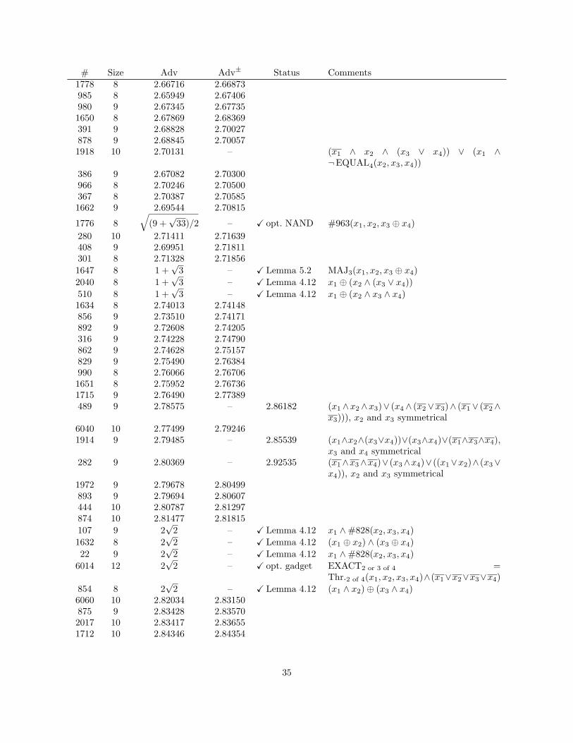
# Size Adv Adv± Status Comments1778 8 2.66716 2.66873985 8 2.65949 2.67406980 9 2.67345 2.677351650 8 2.67869 2.68369391 9 2.68828 2.70027878 9 2.68845 2.700571918 10 2.70131 – (x1 ∧ x2 ∧ (x3 ∨ x4)) ∨ (x1 ∧

¬EQUAL4(x2, x3, x4))386 9 2.67082 2.70300966 8 2.70246 2.70500367 8 2.70387 2.705851662 9 2.69544 2.70815

1776 8√

(9 +√

33)/2 – X opt. NAND #963(x1, x2, x3 ⊕ x4)280 10 2.71411 2.71639408 9 2.69951 2.71811301 8 2.71328 2.718561647 8 1 +

√3 – X Lemma 5.2 MAJ3(x1, x2, x3 ⊕ x4)

2040 8 1 +√

3 – X Lemma 4.12 x1 ⊕ (x2 ∧ (x3 ∨ x4))510 8 1 +

√3 – X Lemma 4.12 x1 ⊕ (x2 ∧ x3 ∧ x4)

1634 8 2.74013 2.74148856 9 2.73510 2.74171892 9 2.72608 2.74205316 9 2.74228 2.74790862 9 2.74628 2.75157829 9 2.75490 2.76384990 8 2.76066 2.767061651 8 2.75952 2.767361715 9 2.76490 2.77389489 9 2.78575 – 2.86182 (x1 ∧x2 ∧x3)∨ (x4 ∧ (x2 ∨x3)∧ (x1 ∨ (x2 ∧

x3))), x2 and x3 symmetrical6040 10 2.77499 2.792461914 9 2.79485 – 2.85539 (x1∧x2∧(x3∨x4))∨(x3∧x4)∨(x1∧x3∧x4),

x3 and x4 symmetrical282 9 2.80369 – 2.92535 (x1∧x3∧x4)∨ (x3∧x4)∨ ((x1∨x2)∧ (x3∨

x4)), x2 and x3 symmetrical1972 9 2.79678 2.80499893 9 2.79694 2.80607444 10 2.80787 2.81297874 10 2.81477 2.81815107 9 2

√2 – X Lemma 4.12 x1 ∧#828(x2, x3, x4)

1632 8 2√

2 – X Lemma 4.12 (x1 ⊕ x2) ∧ (x3 ⊕ x4)22 9 2

√2 – X Lemma 4.12 x1 ∧#828(x2, x3, x4)

6014 12 2√

2 – X opt. gadget EXACT2 or 3 of 4 =Thr.2 of 4(x1, x2, x3, x4)∧(x1∨x2∨x3∨x4)

854 8 2√

2 – X Lemma 4.12 (x1 ∧ x2)⊕ (x3 ∧ x4)6060 10 2.82034 2.83150875 9 2.83428 2.835702017 10 2.83417 2.836551712 10 2.84346 2.84354

35

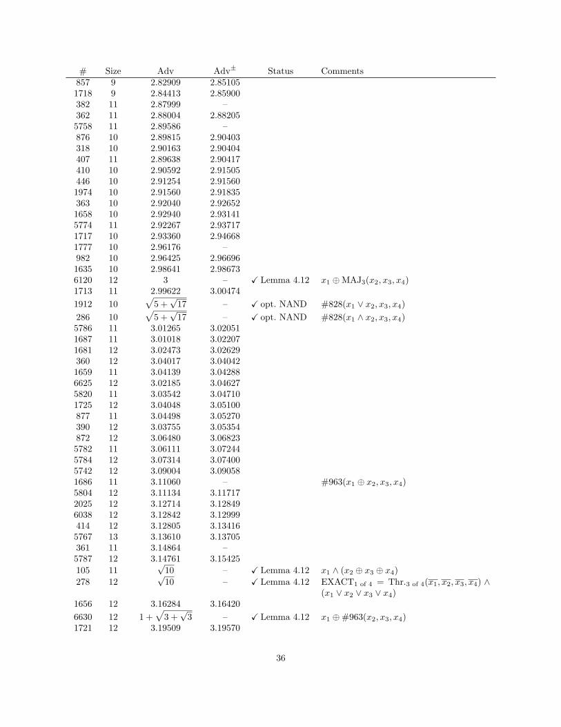
# Size Adv Adv± Status Comments857 9 2.82909 2.851051718 9 2.84413 2.85900382 11 2.87999 –362 11 2.88004 2.882055758 11 2.89586 –876 10 2.89815 2.90403318 10 2.90163 2.90404407 11 2.89638 2.90417410 10 2.90592 2.91505446 10 2.91254 2.915601974 10 2.91560 2.91835363 10 2.92040 2.926521658 10 2.92940 2.931415774 11 2.92267 2.937171717 10 2.93360 2.946681777 10 2.96176 –982 10 2.96425 2.966961635 10 2.98641 2.986736120 12 3 – X Lemma 4.12 x1 ⊕MAJ3(x2, x3, x4)1713 11 2.99622 3.004741912 10

√5 +√

17 – X opt. NAND #828(x1 ∨ x2, x3, x4)286 10

√5 +√

17 – X opt. NAND #828(x1 ∧ x2, x3, x4)5786 11 3.01265 3.020511687 11 3.01018 3.022071681 12 3.02473 3.02629360 12 3.04017 3.040421659 11 3.04139 3.042886625 12 3.02185 3.046275820 11 3.03542 3.047101725 12 3.04048 3.05100877 11 3.04498 3.05270390 12 3.03755 3.05354872 12 3.06480 3.068235782 11 3.06111 3.072445784 12 3.07314 3.074005742 12 3.09004 3.090581686 11 3.11060 – #963(x1 ⊕ x2, x3, x4)5804 12 3.11134 3.117172025 12 3.12714 3.128496038 12 3.12842 3.12999414 12 3.12805 3.134165767 13 3.13610 3.13705361 11 3.14864 –5787 12 3.14761 3.15425105 11

√10 – X Lemma 4.12 x1 ∧ (x2 ⊕ x3 ⊕ x4)

278 12√

10 – X Lemma 4.12 EXACT1 of 4 = Thr.3 of 4(x1, x2, x3, x4) ∧(x1 ∨ x2 ∨ x3 ∨ x4)

1656 12 3.16284 3.164206630 12 1 +

√3 +√

3 – X Lemma 4.12 x1 ⊕#963(x2, x3, x4)1721 12 3.19509 3.19570

36

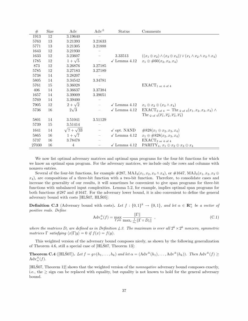
# Size Adv Adv± Status Comments1913 12 3.19640 –5763 13 3.21393 3.216335771 13 3.21305 3.218881643 12 3.21930 –1633 12 3.23607 – 3.33513 ((x1⊕x2)∧ (x3⊕x4))∨ (x1 ∧x2 ∧x3 ∧x4)1785 12 1 +

√5 – X Lemma 4.12 x1 ⊕#60(x2, x3, x4)

873 12 3.26876 3.271855785 12 3.27183 3.271895738 14 3.28207 –5805 14 3.34542 3.347815761 15 3.36028 – EXACT1 or 4 of 4

406 14 3.36637 3.373841657 14 3.39009 3.390515769 14 3.39400 –7905 12 2 +

√2 – X Lemma 4.12 x1 ⊕ x2 ⊕ (x3 ∧ x4)

5736 16 2√

3 – X Lemma 4.12 EXACT2 of 4 = Thr.2 of 4(x1, x2, x3, x4) ∧Thr.2 of 4(x1, x2, x3, x4)

5801 14 3.51041 3.511295739 15 3.51414 –1641 14

√7 +√

33 – X opt. NAND #828(x1 ⊕ x2, x3, x4)5865 16 1 +

√7 – X Lemma 4.12 x1 ⊕#828(x2, x3, x4)

5737 16 3.78478 – EXACT2 or 4 of 4

27030 16 4 – X Lemma 4.12 PARITY4, x1 ⊕ x2 ⊕ x3 ⊕ x4

We now list optimal adversary matrices and optimal span programs for the four-bit functions for whichwe know an optimal span program. For the adversary matrices, we include only the rows and columns withnonzero entries.

Several of the four-bit functions, for example #287, MAJ3(x1, x2, x3 ∧ x4), or #1647, MAJ3(x1, x2, x3 ⊕x4), are compositions of a three-bit function with a two-bit function. Therefore, to consolidate cases andincrease the generality of our results, it will sometimes be convenient to give span programs for three-bitfunctions with unbalanced input complexities. Lemma 5.2, for example, implies optimal span programs forboth functions #287 and #1647. For the adversary lower bound, it is also convenient to define the generaladversary bound with costs [HLS07, HLS05]:

Definition C.3 (Adversary bound with costs). Let f : 0, 1k → 0, 1, and let α ∈ Rn+ be a vector of

positive reals. Define

Adv±α (f) = maxΓ6=0

‖Γ‖maxi 1

αi‖Γ Di‖

, (C.1)

where the matrices Di are defined as in Definition 4.3. The maximum is over all 2k×2k nonzero, symmetricmatrices Γ satisfying 〈x|Γ|y〉 = 0 if f(x) = f(y).

This weighted version of the adversary bound composes nicely, as shown by the following generalizationof Theorem 4.6, still a special case of [HLS07, Theorem 13]:

Theorem C.4 ([HLS07]). Let f = g(h1, . . . , hk) and let α = (Adv±(h1), . . . ,Adv±(hk)). Then Adv±(f) ≥Adv±α (f).

[HLS07, Theorem 12] shows that the weighted version of the nonnegative adversary bound composes exactly,i.e., the ≥ sign can be replaced with equality, but equality is not known to hold for the general adversarybound.

37

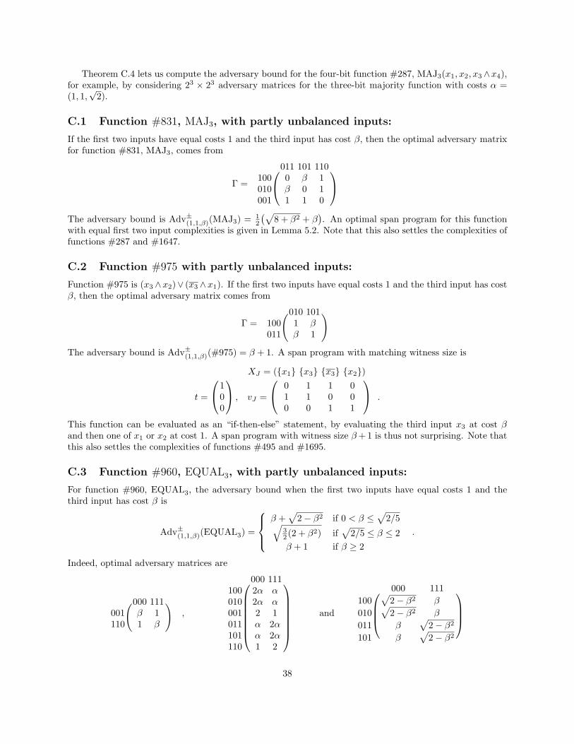
Theorem C.4 lets us compute the adversary bound for the four-bit function #287, MAJ3(x1, x2, x3∧x4),for example, by considering 23 × 23 adversary matrices for the three-bit majority function with costs α =(1, 1,

√2).

C.1 Function #831, MAJ3, with partly unbalanced inputs:

If the first two inputs have equal costs 1 and the third input has cost β, then the optimal adversary matrixfor function #831, MAJ3, comes from

Γ =

011 101 110100 0 β 1010 β 0 1001 1 1 0

The adversary bound is Adv±(1,1,β)(MAJ3) = 12

(√8 + β2 + β

). An optimal span program for this function

with equal first two input complexities is given in Lemma 5.2. Note that this also settles the complexities offunctions #287 and #1647.

C.2 Function #975 with partly unbalanced inputs:

Function #975 is (x3 ∧x2)∨ (x3 ∧x1). If the first two inputs have equal costs 1 and the third input has costβ, then the optimal adversary matrix comes from

Γ =(010 101)

100 1 β011 β 1

The adversary bound is Adv±(1,1,β)(#975) = β + 1. A span program with matching witness size is

XJ = (x1 x3 x3 x2)

t =

1 , vJ =

0 1 1 0 .0 1 1 0 0

0 0 0 1 1

This function can be evaluated as an “if-then-else” statement, by evaluating the third input x3 at cost βand then one of x1 or x2 at cost 1. A span program with witness size β+ 1 is thus not surprising. Note thatthis also settles the complexities of functions #495 and #1695.

C.3 Function #960, EQUAL3, with partly unbalanced inputs:

For function #960, EQUAL3, the adversary bound when the first two inputs have equal costs 1 and thethird input has cost β is

Adv±(1,1,β)(EQUAL3) =

β +

√2− β2 if 0 < β ≤

√2/5√

32 (2 + β2) if

√2/5 ≤ β ≤ 2

β + 1 if β ≥ 2

.

Indeed, optimal adversary matrices are

(000 111)001 β 1110 1 β

,

000 111100 2α α010 2α α001 2 1011 α 2α101 α 2α110 1 2

and

000 111

100√

2− β2 β

010√

2− β2 β

011 β√

2− β2

101 β√

2− β2

38

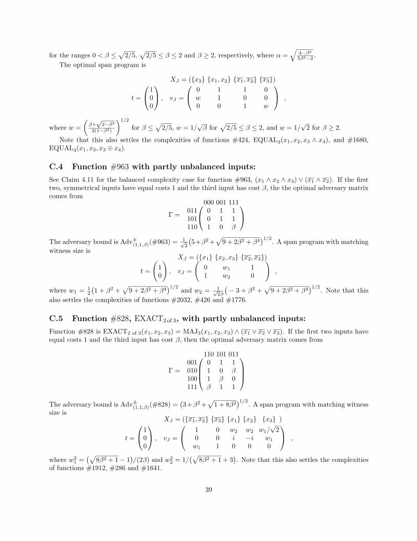
for the ranges 0 < β ≤√

2/5,√

2/5 ≤ β ≤ 2 and β ≥ 2, respectively, where α =√

4−β2

5β2−2 .The optimal span program is

XJ = (x3 x1, x2 x1, x2 x3)

t =

1 , vJ =

0 1 1 0 ,0 w 1 0 0

0 0 0 1 w

where w =(β+√

2−β2

2(1−β2)

)1/2

for β ≤√

2/5, w = 1/√β for

√2/5 ≤ β ≤ 2, and w = 1/

√2 for β ≥ 2.

Note that this also settles the complexities of functions #424, EQUAL3(x1, x2, x3 ∧ x4), and #1680,EQUAL3(x1, x2, x3 ⊕ x4).

C.4 Function #963 with partly unbalanced inputs:

See Claim 4.11 for the balanced complexity case for function #963, (x1 ∧ x2 ∧ x3) ∨ (x1 ∧ x2). If the firsttwo, symmetrical inputs have equal costs 1 and the third input has cost β, the the optimal adversary matrixcomes from

Γ =

000 001 111011 0 1 1101 0 1 1110 1 0 β

The adversary bound is Adv±(1,1,β)(#963) = 1√2

(5+β2 +

√9 + 2β2 + β4

)1/2. A span program with matchingwitness size is

XJ = (x1 x2, x3 x2, x3)

t =

(1), vJ =

(0 w1 1

),

0 1 w2 0

where w1 = 12

(1 + β2 +

√9 + 2β2 + β4

)1/2 and w2 = 1√2β

(− 3 + β2 +

√9 + 2β2 + β4

)1/2. Note that thisalso settles the complexities of functions #2032, #426 and #1776.

C.5 Function #828, EXACT2 of 3, with partly unbalanced inputs:

Function #828 is EXACT2 of 3(x1, x2, x3) = MAJ3(x1, x2, x3) ∧ (x1 ∨ x2 ∨ x3). If the first two inputs haveequal costs 1 and the third input has cost β, then the optimal adversary matrix comes from

Γ =

110 101 011

001 0 1 1010 1 0 β100 1 β 0111 β 1 1

The adversary bound is Adv±(1,1,β)(#828) =(3+β2 +

√1 + 8β2

)1/2. A span program with matching witnesssize is

XJ = (x1, x2 x3 x1 x2 x3 )

t =

1 , vJ =

1 0 w2 w2 w1/√

2 ,0 0 0 i −i w1

0 w1 1 0 0 0

where w21 =

(√8β2 + 1− 1

)/(2β) and w2

2 = 1/(√

8β2 + 1 + 3). Note that this also settles the complexities

of functions #1912, #286 and #1641.

39

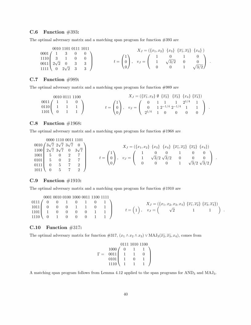
C.6 Function #393:

The optimal adversary matrix and a matching span program for function #393 are

0010 1101 0111 10110001

1 3 0 0

1110 3 1 0 00011 2

√2 0 3 3

1111 0 2√

2 3 3

XJ = (x1, x2 x3 x1, x2 x4 )

t =

1 , vJ =

1 0 1 0 .0 1

√3/2 0 0

0 0 0 1√

3/2

C.7 Function #989:

The optimal adversary matrix and a matching span program for function #989 are

0010 0111 11000011

1 1 00110 1 1 1

1101 0 1 1

XJ = (x1, x2 ∅ x2 x3 x4 x4)

t =

1 , vJ =

0 1 1 1 21/4 1 .0 0 1 2−1/4 2−1/4 1 1

0 21/4 1 0 0 0 0

C.8 Function #1968:

The optimal adversary matrix and a matching span program for function #1968 are

0000 1110 0011 11010010 3

√7 2√

7 3√

7 01100 2

√7 3√

7 0 3√

71001 5 0 2 70101 5 0 2 70111 0 5 7 21011 0 5 7 2

XJ = (x1, x2 x3 x4 x1, x2 x3 x4)

t =

1 , vJ =

1 0 0 1 0 0 .0 1

√3/2√

3/2 0 0 00 0 0 0 1

√3/2√

3/2

C.9 Function #1910:

The optimal adversary matrix and a matching span program for function #1910 are

0001 0010 0100 1000 0011 1100 1111

0111 0 0 1 0 1 0 11011 0 0 0 1 1 0 11101 1 0 0 0 0 1 11110 0 1 0 0 0 1 1

XJ = (x1, x2, x3, x4 x1, x2 x3, x4)t =

(1), vJ =

( √2 1 1

).

C.10 Function #317:

The optimal adversary matrix for function #317, (x1 ∧ x2 ∧ x3) ∨MAJ3(x2, x3, x4), comes from

Γ =

0111 1010 1100

1000 0 1 10011 1 1 00101 1 0 11110 1 1 1

A matching span program follows from Lemma 4.12 applied to the span programs for AND3 and MAJ3.

40

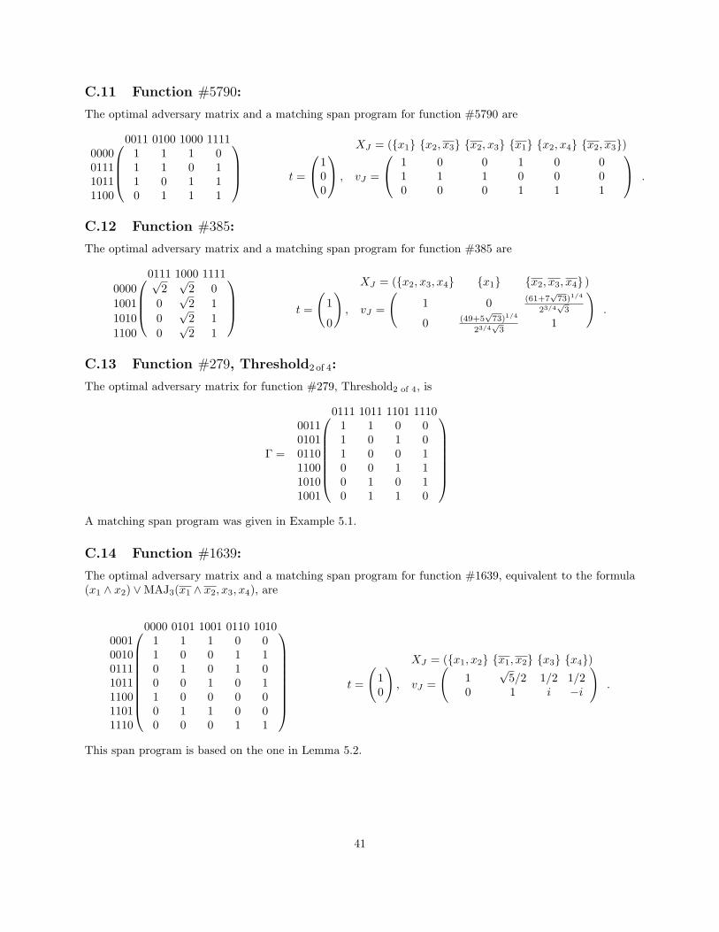
C.11 Function #5790:

The optimal adversary matrix and a matching span program for function #5790 are

0011 0100 1000 1111

0000 1 1 1 00111 1 1 0 11011 1 0 1 11100 0 1 1 1

XJ = (x1 x2, x3 x2, x3 x1 x2, x4 x2, x3)

t =

1 , vJ =

1 0 0 1 0 0 .0 1 1 1 0 0 0

0 0 0 0 1 1 1

C.12 Function #385:

The optimal adversary matrix and a matching span program for function #385 are

0111 1000 1111

0000√

2√

2 01001 0

√2 1

1010 0√

2 11100 0

√2 1

XJ = (x2, x3, x4 x1 x2, x3, x4 )

t =

(1), vJ =

(1 0 (61+7

√73)1/4

23/4√

3

).

0 0 (49+5√

73)1/4

23/4√

31

C.13 Function #279, Threshold2 of 4:

The optimal adversary matrix for function #279, Threshold2 of 4, is

Γ =

0111 1011 1101 11100011 1 1 0 00101 1 0 1 00110 1 0 0 11100 0 0 1 11010 0 1 0 11001 0 1 1 0

A matching span program was given in Example 5.1.

C.14 Function #1639:

The optimal adversary matrix and a matching span program for function #1639, equivalent to the formula(x1 ∧ x2) ∨MAJ3(x1 ∧ x2, x3, x4), are

0000 0101 1001 0110 1010

0001 1 1 1 0 00010 1 0 0 1 10111 0 1 0 1 01011 0 0 1 0 11100 1 0 0 0 01101 0 1 1 0 01110 0 0 0 1 1

XJ = (x1, x2 x1, x2 x3 x4)

t =

(1), vJ =

(1

√5/2 1/2 1/2

).

0 0 1 i −i

This span program is based on the one in Lemma 5.2.

41

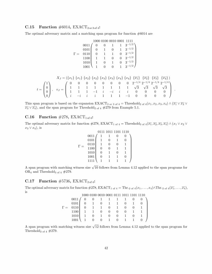
C.15 Function #6014, EXACT2 or 3 of 4:

The optimal adversary matrix and a matching span program for function #6014 are

Γ =

1000 0100 0010 0001 1111 0011 0 0 1 1 3−1/2

0101 0 1 0 1 3−1/2

0110 0 1 1 0 3−1/2

1100 1 1 0 0 3−1/2

1010 1 0 1 0 3−1/2

1001 1 0 0 1 3−1/2

XJ = (x1 x1 x2 x2 x3 x3 x4 x4 x1 x2 x3 x4 )

t =

1 , vJ =

0 0 0 0 0 0 0 0 2−1/4 2−1/4 2−1/4 2−1/4

.0 1 1 1 1 1 1 1 1

√3√

3√

3√

30 1 1 1 −1 i −i i i 0 0 0 00 i −i i i 1 1 1 −1 0 0 0 0

This span program is based on the expansion EXACT2 or 3 of 4 = Threshold2 of 4(x1, x2, x3, x4) ∧ (x1 ∨ x2 ∨x3 ∨ x4), and the span program for Threshold2 of 4 #279 from Example 5.1.

C.16 Function #278, EXACT1 of 4:

The optimal adversary matrix for function #278, EXACT1 of 4 = Threshold3 of 4(x1, x2, x3, x4) ∧ (x1 ∨ x2 ∨x3 ∨ x4), is

Γ =

0111 1011 1101 1110

0011 1 1 0 00101 1 0 1 00110 1 0 0 11100 0 0 1 11010 0 1 0 11001 0 1 1 01111 1 1 1 1

A span program with matching witness size√

10 follows from Lemma 4.12 applied to the span programs forOR4 and Threshold3 of 4 #279.

C.17 Function #5736, EXACT2 of 4:

The optimal adversary matrix for function #278, EXACT1 of 4 = Thr.2 of 4(x1, . . . , x4)∧Thr.2 of 4(x1, . . . , x4),is

Γ =

1000 0100 0010 0001 0111 1011 1101 11100011 0 0 1 1 1 1 0 00101 0 1 0 1 1 0 1 00110 0 1 1 0 1 0 0 11100 1 1 0 0 0 0 1 11010 1 0 1 0 0 1 0 11001 1 0 0 1 0 1 1 0

A span program with matching witness size√

12 follows from Lemma 4.12 applied to the span program forThreshold2 of 4 #279.

42