Spam Filtering based on Naive Bayes Classification

Tianhao Sun

May 1, 2009

Abstract

This project discusses about the popular statistical spam filtering pro-cess: naive Bayes classification. A fairly famous way of implementing thenaive Bayes method in spam filtering by Paul Graham is explored and aadjustment of this method from Tim Peter is evaluated based on applica-tions on real data. Two solutions to the problem of unknown tokens arealso tested on the sample emails. The last part of the project shows how theBayesian noise reduction algorithm can improve the accuracy of the naiveBayes classification.

Declaration

This piece of work is a result of my own work except where it forms anassessment based on group project work. In the case of a group project,the work has been prepared in collaboration with other members of thegroup. Material from the work of others not involved in the project hasbeen acknowledged and quotations and paraphrases suitably indicated.

1

Contents

1 Introduction 3

2 Naive Bayes Classification 52.1 Training data . . . . . . . . . . . . . . . . . . . . . . . . . . . 52.2 Filtering process . . . . . . . . . . . . . . . . . . . . . . . . . 72.3 Application . . . . . . . . . . . . . . . . . . . . . . . . . . . . 10

3 Paul Graham’s Method 123.1 Filtering process . . . . . . . . . . . . . . . . . . . . . . . . . 123.2 Application . . . . . . . . . . . . . . . . . . . . . . . . . . . . 153.3 Tim Peter’s criticism . . . . . . . . . . . . . . . . . . . . . . . 19

4 Unknown Tokens 244.1 Modified sample emails . . . . . . . . . . . . . . . . . . . . . 244.2 Problem . . . . . . . . . . . . . . . . . . . . . . . . . . . . . . 244.3 Solution . . . . . . . . . . . . . . . . . . . . . . . . . . . . . . 254.4 Application . . . . . . . . . . . . . . . . . . . . . . . . . . . . 27

5 Bayesian Noise Reduction 335.1 Introduction . . . . . . . . . . . . . . . . . . . . . . . . . . . . 335.2 Zdziarski’s BNR algorithm . . . . . . . . . . . . . . . . . . . . 335.3 Application . . . . . . . . . . . . . . . . . . . . . . . . . . . . 35

6 Conclusion 39

2

Chapter 1

Introduction

In this project, I investigate one of the widely used statistical spam filters,Bayesian spam filters. The first known mail-filtering program to use a Bayesclassifier was Jason Rennie’s iFile program, released in 1996. The first schol-arly publication on Bayesian spam filtering was by Sahami et al. (1998)[12].A naive Bayes classifier[3] simply apply Bayes’ theorem on the context clas-sification of each email, with a strong assumption that the words included inthe email are independent to each other. In the beginning, we will get twosample emails from the real life data in order to create the training dataset.Then a detailed filtering process of the naive Bayes classification will beexplained and we will apply this method on our sample emails for testing inthe end of the chapter. These sample emails will be tested throughout theproject using the other methods we will discuss about later.

Among all the different ways of implementing naive Bayes classification,Paul Graham’s approach has become fairly famous[2]. He introduced a newformula for calculating token values and overall probabilities of an emailbeing classified as spam. But there is a unrealistic assumption in his formulawhich assume the number of spam and ham are equal in the dataset foreveryone. Where Tim Peter correctly adjust the formula later to make it fitinto all datasets[7], and both methods will be evaluated using our trainingdataset.

Also two different solutions to the problem of unknown tokens will bediscussed in this project, the simple one is introduced by Paul Grahamand the more accurate approach is created by Gary Robinson[10]. WhereRobinson’s method lets us consider both our background knowledge andthe limited data we have got from unknown tokens in the prediction of theirtoken values. Again, their performances will be measured against our sampleemails.

Then, we will discuss about a major improvement on the Bayesian filter-ing process: Bayesian noise reduction. Jonathan A. Zdziarski first discussedabout the Bayesian noise reduction algorithm in 2004[15], and also include

3

this idea in his book later[16, p. 231]. The BNR algorithm is particularlyuseful in making the filtering process more effective and gain a higher levelof confidence in the classification.

4

Chapter 2

Naive Bayes Classification

2.1 Training data

Here I want to introduce some email examples to demonstrate the processof naive Bayes classification. Each of them contains 15 words or tokens inthe filtering way of saying, and all of them will be included in the trainingdata table later on.

• Example for spam:

Paying too much for VIAGRA?

Now,you have a chance to receive a FREE TRIAL!

• Example for ham:

For the Clarins, just take your time. As i have advised her to exerciseregularly.

The following table is made to show the frequency of a token appearin both email groups, the appearances of each token count only once foreach email received. I estimated these word counts based on some previouswork done by Vasanth Elavarasan[1] and the book written by Jonathan A.Zdziarski[16, p. 65]. Due to the email group size for Zdziarski’s word countslist is smaller than Elanvarasan’s, I only took the ratio factor into accountand reproduced the new word counts according to our dataset. For example,tokens such as The, Vehicle and Viagra are not included in Elavarasan’s wordlist. In order to make use of Zdziarski’s data, I simply multiply the ratio inhis dataset by the total number in the new table. Here is how I get the newfrequencies for these three tokens.(Table 2.1) Note the training dataset herehas a total number of 432 spam and 2170 ham.(Table 2.2)

5

The 96/224× 432 ≈ 185 48/112× 2170 ≈ 930Vehicle 11/224× 432 ≈ 21 3/112× 2170 ≈ 58Viagra 20/224× 432 ≈ 39 1/112× 2170 ≈ 19

Table 2.1: Table of estimated data

Feature Appearances in Spam Appearances in HamA 165 1235Advised 12 42As 2 579Chance 45 35Clarins 1 6Exercise 6 39For 378 1829Free 253 137Fun 59 9Girlfriend 26 8Have 291 2008Her 38 118I 9 1435Just 207 253Much 126 270Now 221 337Paying 26 10Receive 171 98Regularly 9 87Take 142 287Tell 76 89The 185 930Time 212 446To 389 1948Too 56 141Trial 26 13Vehicle 21 58Viagra 39 19You 391 786Your 332 450

Table 2.2: Table of training data

6

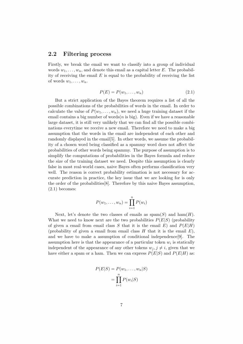
2.2 Filtering process

Firstly, we break the email we want to classify into a group of individualwords w1, . . . , wn, and denote this email as a capital letter E. The probabil-ity of receiving the email E is equal to the probability of receiving the listof words w1, . . . , wn.

P (E) = P (w1, . . . , wn) (2.1)

But a strict application of the Bayes theorem requires a list of all thepossible combinations of the probabilities of words in the email. In order tocalculate the value of P (w1, . . . , wn), we need a huge training dataset if theemail contains a big number of words(n is big). Even if we have a reasonablelarge dataset, it is still very unlikely that we can find all the possible combi-nations everytime we receive a new email. Therefore we need to make a bigassumption that the words in the email are independent of each other andrandomly displayed in the email[5]. In other words, we assume the probabil-ity of a chosen word being classified as a spammy word does not affect theprobabilities of other words being spammy. The purpose of assumption is tosimplify the computations of probabilities in the Bayes formula and reducethe size of the training dataset we need. Despite this assumption is clearlyfalse in most real-world cases, naive Bayes often performs classification verywell. The reason is correct probability estimation is not necessary for ac-curate prediction in practice, the key issue that we are looking for is onlythe order of the probabilities[8]. Therefore by this naive Bayes assumption,(2.1) becomes:

P (w1, . . . , wn) =n∏

i=1

P (wi)

Next, let’s denote the two classes of emails as spam(S) and ham(H).What we need to know next are the two probabilities P (E|S) (probabilityof given a email from email class S that it is the email E) and P (E|H)(probability of given a email from email class H that it is the email E),and we have to make a assumption of conditional independence[9]. Theassumption here is that the appearance of a particular token wi is staticallyindependent of the appearance of any other tokens wj , j 6= i, given that wehave either a spam or a ham. Then we can express P (E|S) and P (E|H) as:

P (E|S) = P (w1, . . . , wn|S)

=n∏

i=1

P (wi|S)

7

and

P (E|H) = P (w1, . . . , wn|H)

=n∏

i=1

P (wi|H)

The reason that we set up a training dataset is to estimate how spammyeach word is, where probabilities P (wi|S)(probability of given a email fromemail class S which it contains the word wi) and P (wi|H)(probability ofgiven a email from email class H which it contains the word wi) are needed.They denote the conditional probability that a given email contains theword wi under the assumption that this email is spam or ham respectively.We estimate these probabilities by calculating the frequencies of the wordsappear in either groups of emails from the training dataset. In the followingformula, P (wi∩S) is the probability that a given email is a spam email andcontains the word wi. Thus, by Bayes theorem:

P (wi|S) =P (wi ∩ S)P (S)

and P (wi|H) =P (wi ∩H)P (H)

For example,the word Free in our training dataset:

P (w8 ∩ S) =253

432 + 2170

and

P (S) =432

432 + 2170

thus, we get

P (w8|S) =253432

The following step is to compute the posterior probability of spam emailgiven the overall probability of the sampling email by Bayes’ rule, this is thecrucial part of the entire classification.

P (S|E) =P (E|S)P (S)

P (E)(2.2)

=P (S)

n∏i=1

P (wi|S)

P (E)

8

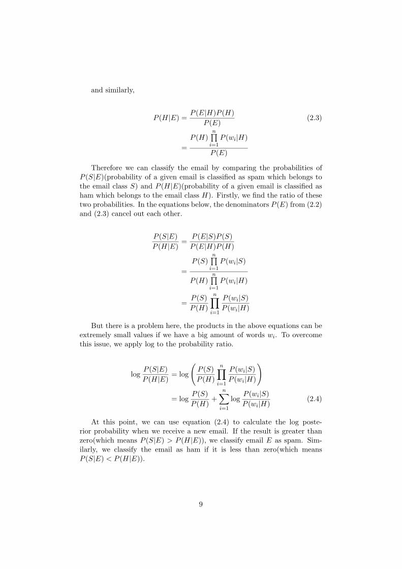
and similarly,

P (H|E) =P (E|H)P (H)

P (E)(2.3)

=P (H)

n∏i=1

P (wi|H)

P (E)

Therefore we can classify the email by comparing the probabilities ofP (S|E)(probability of a given email is classified as spam which belongs tothe email class S) and P (H|E)(probability of a given email is classified asham which belongs to the email class H). Firstly, we find the ratio of thesetwo probabilities. In the equations below, the denominators P (E) from (2.2)and (2.3) cancel out each other.

P (S|E)P (H|E)

=P (E|S)P (S)P (E|H)P (H)

=P (S)

n∏i=1

P (wi|S)

P (H)n∏

i=1P (wi|H)

=P (S)P (H)

n∏i=1

P (wi|S)P (wi|H)

But there is a problem here, the products in the above equations can beextremely small values if we have a big amount of words wi. To overcomethis issue, we apply log to the probability ratio.

logP (S|E)P (H|E)

= log

(P (S)P (H)

n∏i=1

P (wi|S)P (wi|H)

)

= logP (S)P (H)

+n∑

i=1

logP (wi|S)P (wi|H)

(2.4)

At this point, we can use equation (2.4) to calculate the log poste-rior probability when we receive a new email. If the result is greater thanzero(which means P (S|E) > P (H|E)), we classify email E as spam. Sim-ilarly, we classify the email as ham if it is less than zero(which meansP (S|E) < P (H|E)).

9

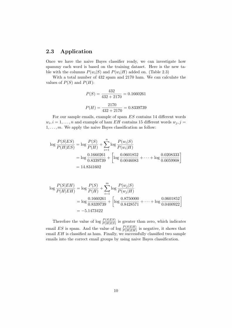
2.3 Application

Once we have the naive Bayes classifier ready, we can investigate howspammy each word is based on the training dataset. Here is the new ta-ble with the columns P (wi|S) and P (wi|H) added on. (Table 2.3)

With a total number of 432 spam and 2170 ham. We can calculate thevalues of P (S) and P (H):

P (S) =432

432 + 2170= 0.1660261

P (H) =2170

432 + 2170= 0.8339739

For our sample emails, example of spam ES contains 14 different wordswi, i = 1, . . . , n and example of ham EH contains 15 different words wj , j =1, . . . ,m. We apply the naive Bayes classification as follow:

logP (S|ES)P (H|ES)

= logP (S)P (H)

+n∑

i=1

logP (wi|S)P (wi|H)

= log0.16602610.8339739

+[log

0.06018520.0046083

+ · · ·+ log0.02083330.0059908

]= 14.8341602

logP (S|EH)P (H|EH)

= logP (S)P (H)

+m∑

i=1

logP (wj |S)P (wj |H)

= log0.16602610.8339739

+[log

0.87500000.8428571

+ · · ·+ log0.06018520.0400922

]= −5.1473422

Therefore the value of log P (S|ES)P (H|ES) is greater than zero, which indicates

email ES is spam. And the value of log P (S|EH)P (H|EH) is negative, it shows that

email EH is classified as ham. Finally, we successfully classified two sampleemails into the correct email groups by using naive Bayes classification.

10

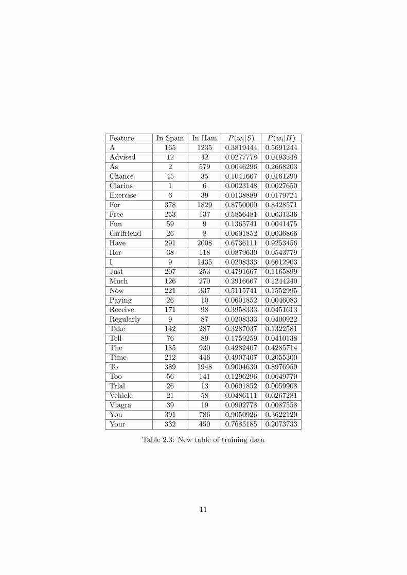
Feature In Spam In Ham P (wi|S) P (wi|H)A 165 1235 0.3819444 0.5691244Advised 12 42 0.0277778 0.0193548As 2 579 0.0046296 0.2668203Chance 45 35 0.1041667 0.0161290Clarins 1 6 0.0023148 0.0027650Exercise 6 39 0.0138889 0.0179724For 378 1829 0.8750000 0.8428571Free 253 137 0.5856481 0.0631336Fun 59 9 0.1365741 0.0041475Girlfriend 26 8 0.0601852 0.0036866Have 291 2008 0.6736111 0.9253456Her 38 118 0.0879630 0.0543779I 9 1435 0.0208333 0.6612903Just 207 253 0.4791667 0.1165899Much 126 270 0.2916667 0.1244240Now 221 337 0.5115741 0.1552995Paying 26 10 0.0601852 0.0046083Receive 171 98 0.3958333 0.0451613Regularly 9 87 0.0208333 0.0400922Take 142 287 0.3287037 0.1322581Tell 76 89 0.1759259 0.0410138The 185 930 0.4282407 0.4285714Time 212 446 0.4907407 0.2055300To 389 1948 0.9004630 0.8976959Too 56 141 0.1296296 0.0649770Trial 26 13 0.0601852 0.0059908Vehicle 21 58 0.0486111 0.0267281Viagra 39 19 0.0902778 0.0087558You 391 786 0.9050926 0.3622120Your 332 450 0.7685185 0.2073733

Table 2.3: New table of training data

11

Chapter 3

Paul Graham’s Method

3.1 Filtering process

Paul Graham has a slightly different way of implementing naive Bayesmethod on spam classifications.[2] His training dataset also contains twogroups of emails, one for spam and the other for ham. The difference is thatthe size of his groups are almost the same, each has about 4000 emails in it.And not like the sample emails I created in the last chapter, which only havemessage bodies, he takes into account the header, javascript and embeddedhtml in each email. For better filtering, he enlarges the domain of tokens byconsidering alphanumeric characters, dashes, apostrophes, and dollar signsas tokens, and all the others as token separators. Of course, more symbolswill be discovered as useful indicators of spam in the future. But at thattime, he ignores purely digits tokens, and html comments.

The filtering process begin with generating the same table as Table 2.2,which states the number of appearance of each token in both email groups.Again, the appearances of each token count only once for each email re-ceived. After that, he calculates the probability of each token that an emailcontaining it is a spam[16, p. 69]. Now, we denote AS and AH as the to-ken’s frequency of appearances in spam and ham respectively. By using ourtraining dataset, the probability P (S|wi) of a token will be computed asfollow:

P (S|wi) =AS/432

AS/432 +AH/2170

For example,the probability of the token Exercise will be:

P (S|w6) =6/432

6/432 + 39/2170= 0.4359180

In this case, the word Exercise is considered as a hammy word whereprobability 0.5 is neutral.

12

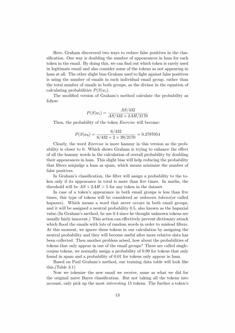
Here, Graham discovered two ways to reduce false positives in the clas-sification. One way is doubling the number of appearances in ham for eachtoken in the email. By doing this, we can find out which token is rarely usedin legitimate email and also consider some of the tokens as not appearing inham at all. The other slight bias Graham used to fight against false positivesis using the number of emails in each individual email group, rather thanthe total number of emails in both groups, as the divisor in the equation ofcalculating probabilities P (S|wi).

The modified version of Graham’s method calculate the probability asfollow:

P (S|wi) =AS/432

AS/432 + 2AH/2170Then, the probability of the token Exercise will become:

P (S|w6) =6/432

6/432 + 2× 39/2170= 0.2787054

Clearly, the word Exercise is more hammy in this version as the prob-ability is closer to 0. Which shows Graham is trying to enhance the effectof all the hammy words in the calculation of overall probability by doublingtheir appearances in ham. This slight bias will help reducing the probabilitythat filters misjudge a ham as spam, which means minimize the number offalse positives.

In Graham’s classification, the filter will assign a probability to the to-ken only if its appearance in total is more than five times. In maths, thethreshold will be AS + 2AH > 5 for any token in the dataset.

In case of a token’s appearance in both email groups is less than fivetimes, this type of tokens will be considered as unknown tokens(or calledhapaxes). Which means a word that never occurs in both email groups,and it will be assigned a neutral probability 0.5, also known as the hapaxialvalue.(In Graham’s method, he use 0.4 since he thought unknown tokens areusually fairly innocent.) This action can effectively prevent dictionary attackwhich flood the emails with lots of random words in order to mislead filters.At this moment, we ignore these tokens in our calculation by assigning theneutral probability and they will become useful after more relative data hasbeen collected. Then another problem arised, how about the probabilities oftokens that only appear in one of the email groups? These are called single-corpus tokens, we normally assign a probability of 0.99 for tokens that onlyfound in spam and a probability of 0.01 for tokens only appear in ham.

Based on Paul Graham’s method, our training data table will look likethis.(Table 3.1)

Now we tokenize the new email we receive, same as what we did forthe original naive Bayes classification. But not taking all the tokens intoaccount, only pick up the most interesting 15 tokens. The further a token’s

13

Feature Appearances in Spam Appearances in Ham P (S|wi)A 165 1235 0.2512473Advised 12 42 0.4177898As 2 579 0.0086009Chance 45 35 0.7635468Clarins 1 6 0.2950775Exercise 6 39 0.2787054For 378 1829 0.3417015Free 253 137 0.8226372Fun 59 9 0.9427419Girlfriend 26 8 0.8908609Have 291 2008 0.2668504Her 38 118 0.4471509I 9 1435 0.0155078Just 207 253 0.6726596Much 126 270 0.5396092Now 221 337 0.6222218Paying 26 10 0.8671995Receive 171 98 0.8142107Regularly 9 87 0.2062346Take 142 287 0.5541010Tell 76 89 0.6820062The 185 930 0.3331618Time 212 446 0.5441787To 389 1948 0.3340176Too 56 141 0.4993754Trial 26 13 0.8339739Vehicle 21 58 0.4762651Viagra 39 19 0.8375393You 391 786 0.5554363Your 332 450 0.6494897

Table 3.1: Training data table with Paul Graham’s method

14

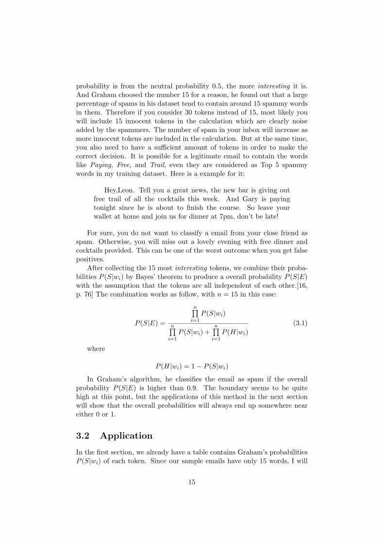
probability is from the neutral probability 0.5, the more interesting it is.And Graham choosed the number 15 for a reason, he found out that a largepercentage of spams in his dataset tend to contain around 15 spammy wordsin them. Therefore if you consider 30 tokens instead of 15, most likely youwill include 15 innocent tokens in the calculation which are clearly noiseadded by the spammers. The number of spam in your inbox will increase asmore innocent tokens are included in the calculation. But at the same time,you also need to have a sufficient amount of tokens in order to make thecorrect decision. It is possible for a legitimate email to contain the wordslike Paying, Free, and Trail, even they are considered as Top 5 spammywords in my training dataset. Here is a example for it:

Hey,Leon. Tell you a great news, the new bar is giving outfree trail of all the cocktails this week. And Gary is payingtonight since he is about to finish the course. So leave yourwallet at home and join us for dinner at 7pm, don’t be late!

For sure, you do not want to classify a email from your close friend asspam. Otherwise, you will miss out a lovely evening with free dinner andcocktails provided. This can be one of the worst outcome when you get falsepositives.

After collecting the 15 most interesting tokens, we combine their proba-bilities P (S|wi) by Bayes’ theorem to produce a overall probability P (S|E)with the assumption that the tokens are all independent of each other.[16,p. 76] The combination works as follow, with n = 15 in this case:

P (S|E) =

n∏i=1

P (S|wi)

n∏i=1

P (S|wi) +n∏

i=1P (H|wi)

(3.1)

where

P (H|wi) = 1− P (S|wi)

In Graham’s algorithm, he classifies the email as spam if the overallprobability P (S|E) is higher than 0.9. The boundary seems to be quitehigh at this point, but the applications of this method in the next sectionwill show that the overall probabilities will always end up somewhere neareither 0 or 1.

3.2 Application

In the first section, we already have a table contains Graham’s probabilitiesP (S|wi) of each token. Since our sample emails have only 15 words, I will

15

Feature In Spam In Ham P (S|wi) InterestingnessPaying 26 10 0.8671995 0.3671995Viagra 39 19 0.8375393 0.3375393Trial 26 13 0.8339739 0.3339739Free 253 137 0.8226372 0.3226372Receive 171 98 0.8142107 0.3142107Chance 45 35 0.7635468 0.2635468A 165 1235 0.2512473 0.2487527Have 291 2008 0.2668504 0.2331496To 389 1948 0.3340176 0.1659824For 378 1829 0.3417015 0.1582985Now 221 337 0.6222218 0.1222218You 391 786 0.5554363 0.0554363Much 126 270 0.5396092 0.0396092Too 56 141 0.4993754 0.0006246

Table 3.2: Ordered training data table for sample spam

Feature In Spam In Ham P (S|wi) InterestingnessAs 2 579 0.0086009 0.4913991I 9 1435 0.0155078 0.4844922Regularly 9 87 0.2062346 0.2937654Have 291 2008 0.2668504 0.2331496Exercise 6 39 0.2787054 0.2212946Clarins 1 6 0.2950775 0.2049225Just 207 253 0.6726596 0.1726596The 185 930 0.3331618 0.1668382To 389 1948 0.3340176 0.1659824For 378 1829 0.3417015 0.1582985Your 332 450 0.6494897 0.1494897Advised 12 42 0.4177898 0.0822102Take 142 287 0.5541010 0.0541010Her 38 118 0.4471509 0.0528491Time 212 446 0.5441787 0.0441787

Table 3.3: Ordered training data table for sample ham

16

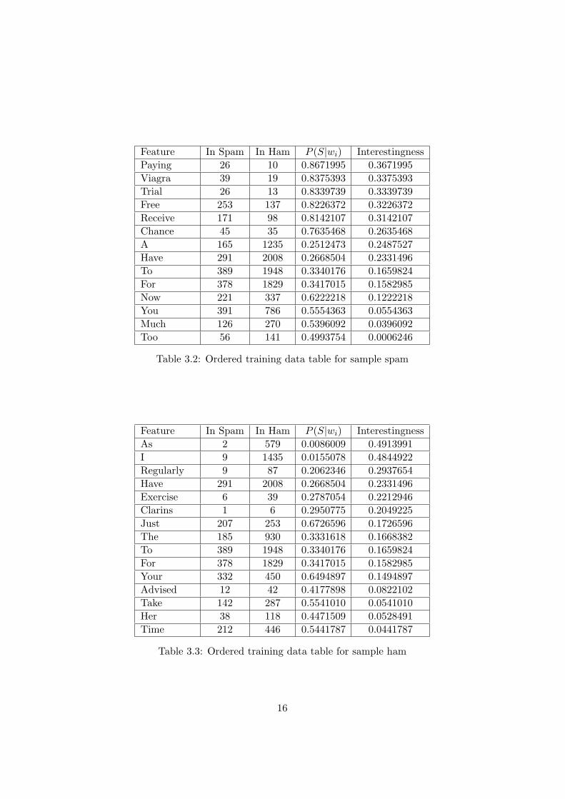
include all the tokens in the calculation first and see how it works. Butin order to attain the best information of the testing email, I decide toadd another column into the table, which measures the Interestingness ofeach token. I rearrange the order of each token by its absolute value ofP (S|wi)− 0.5, which directly shows us how hammy or spammy each tokenis, and how much effect each token contribute to the calculation of the overallprobability. Above is the ordered training data tables for the sample spamand ham: (Table 3.2 and Table 3.3)

Before we do any statistical combination of these token probabilities,let’s have a brief look at the tables first. For the table of sample spam, fiveout of fourteen words are considered hammy words since their probabilitiesare less than 0.5. But at the same time, all of the top five most interestingwords are very spammy with probabilities exceed 0.8. And plus the otherfour spammy words left in the table, we can simply make a decision for theclassification already. Similarly, the sample ham contains only four spammywords in the entire message. And the top six most interesting words are alsohammy words with token probabilities less than 0.3. Therefore it is verystraight forward for a real person to classify the email with these tables, butcomputer needs a more logical way to do that.

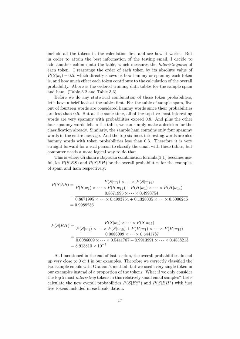
This is where Graham’s Bayesian combination formula(3.1) becomes use-ful, let P (S|ES) and P (S|EH) be the overall probabilities for the examplesof spam and ham respectively:

P (S|ES) =P (S|w1)× · · · × P (S|w14)

P (S|w1)× · · · × P (S|w14) + P (H|w1)× · · · × P (H|w14)

=0.8671995× · · · × 0.4993754

0.8671995× · · · × 0.4993754 + 0.1328005× · · · × 0.5006246= 0.9988236

P (S|EH) =P (S|w1)× · · · × P (S|w15)

P (S|w1)× · · · × P (S|w15) + P (H|w1)× · · · × P (H|w15)

=0.0086009× · · · × 0.5441787

0.0086009× · · · × 0.5441787 + 0.9913991× · · · × 0.4558213= 8.913810× 10−7

As I mentioned in the end of last section, the overall probabilities do endup very close to 0 or 1 in our examples. Therefore we correctly classified thetwo sample emails with Graham’s method, but we used every single token inour examples instead of a proportion of the tokens. What if we only considerthe top 5 most interesting tokens in this relatively small email samples? Let’scalculate the new overall probabilities P (S|ES∗) and P (S|EH∗) with justfive tokens included in each calculation.

17

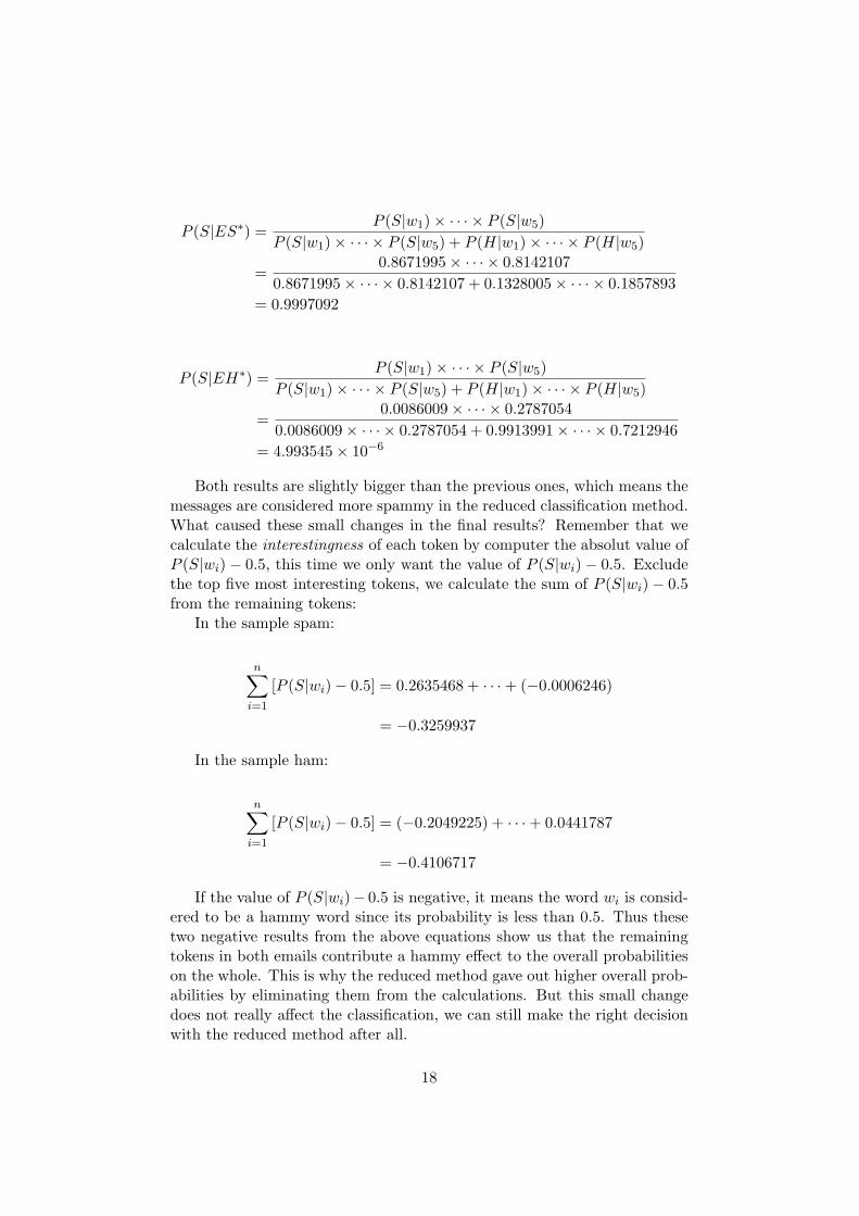
P (S|ES∗) =P (S|w1)× · · · × P (S|w5)

P (S|w1)× · · · × P (S|w5) + P (H|w1)× · · · × P (H|w5)

=0.8671995× · · · × 0.8142107

0.8671995× · · · × 0.8142107 + 0.1328005× · · · × 0.1857893= 0.9997092

P (S|EH∗) =P (S|w1)× · · · × P (S|w5)

P (S|w1)× · · · × P (S|w5) + P (H|w1)× · · · × P (H|w5)

=0.0086009× · · · × 0.2787054

0.0086009× · · · × 0.2787054 + 0.9913991× · · · × 0.7212946= 4.993545× 10−6

Both results are slightly bigger than the previous ones, which means themessages are considered more spammy in the reduced classification method.What caused these small changes in the final results? Remember that wecalculate the interestingness of each token by computer the absolut value ofP (S|wi)− 0.5, this time we only want the value of P (S|wi)− 0.5. Excludethe top five most interesting tokens, we calculate the sum of P (S|wi)− 0.5from the remaining tokens:

In the sample spam:

n∑i=1

[P (S|wi)− 0.5] = 0.2635468 + · · ·+ (−0.0006246)

= −0.3259937

In the sample ham:

n∑i=1

[P (S|wi)− 0.5] = (−0.2049225) + · · ·+ 0.0441787

= −0.4106717

If the value of P (S|wi)− 0.5 is negative, it means the word wi is consid-ered to be a hammy word since its probability is less than 0.5. Thus thesetwo negative results from the above equations show us that the remainingtokens in both emails contribute a hammy effect to the overall probabilitieson the whole. This is why the reduced method gave out higher overall prob-abilities by eliminating them from the calculations. But this small changedoes not really affect the classification, we can still make the right decisionwith the reduced method after all.

18

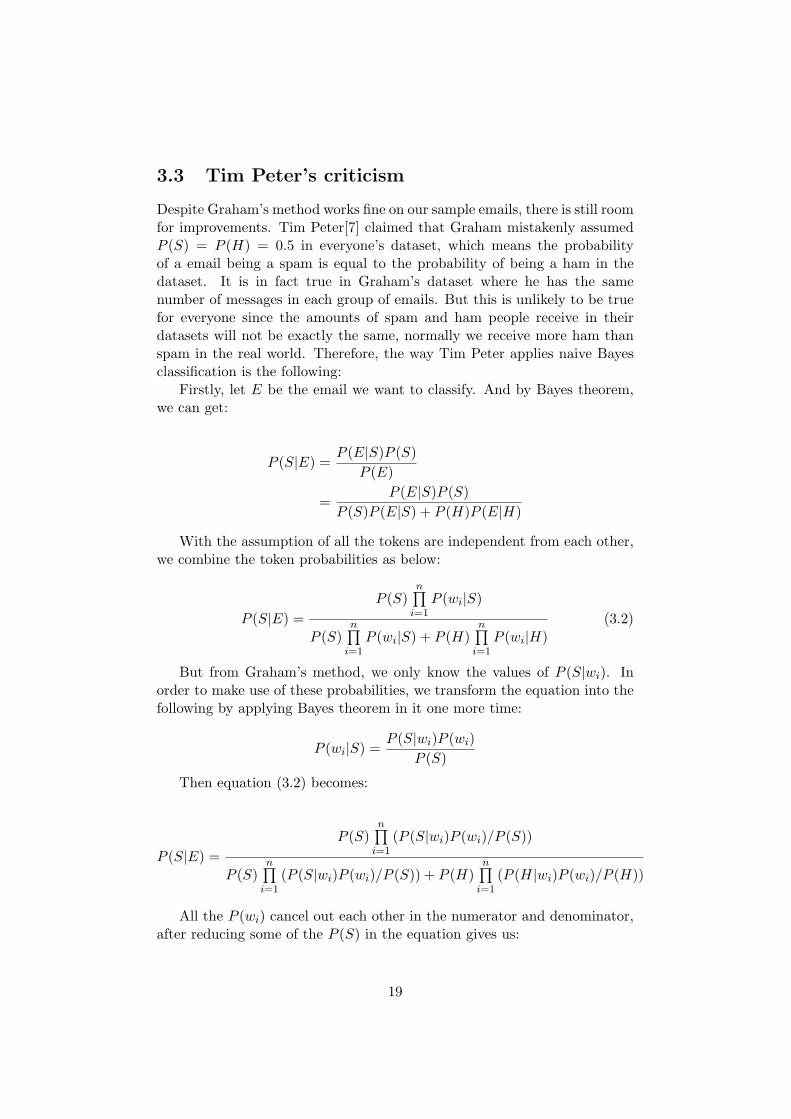
3.3 Tim Peter’s criticism

Despite Graham’s method works fine on our sample emails, there is still roomfor improvements. Tim Peter[7] claimed that Graham mistakenly assumedP (S) = P (H) = 0.5 in everyone’s dataset, which means the probabilityof a email being a spam is equal to the probability of being a ham in thedataset. It is in fact true in Graham’s dataset where he has the samenumber of messages in each group of emails. But this is unlikely to be truefor everyone since the amounts of spam and ham people receive in theirdatasets will not be exactly the same, normally we receive more ham thanspam in the real world. Therefore, the way Tim Peter applies naive Bayesclassification is the following:

Firstly, let E be the email we want to classify. And by Bayes theorem,we can get:

P (S|E) =P (E|S)P (S)

P (E)

=P (E|S)P (S)

P (S)P (E|S) + P (H)P (E|H)

With the assumption of all the tokens are independent from each other,we combine the token probabilities as below:

P (S|E) =P (S)

n∏i=1

P (wi|S)

P (S)n∏

i=1P (wi|S) + P (H)

n∏i=1

P (wi|H)(3.2)

But from Graham’s method, we only know the values of P (S|wi). Inorder to make use of these probabilities, we transform the equation into thefollowing by applying Bayes theorem in it one more time:

P (wi|S) =P (S|wi)P (wi)

P (S)

Then equation (3.2) becomes:

P (S|E) =P (S)

n∏i=1

(P (S|wi)P (wi)/P (S))

P (S)n∏

i=1(P (S|wi)P (wi)/P (S)) + P (H)

n∏i=1

(P (H|wi)P (wi)/P (H))

All the P (wi) cancel out each other in the numerator and denominator,after reducing some of the P (S) in the equation gives us:

19

P (S|E) =P (S)1−n

n∏i=1

P (S|wi)

P (S)1−nn∏

i=1P (S|wi) + P (H)1−n

n∏i=1

P (H|wi)(3.3)

This is obviously different from Graham’s formula (3.1), his formula doesnot include the terms P (S)1−n and P (H)1−n. The reason is that P (S) =P (H) in Graham’s method, they will be canceled out in the equation. Thisis clearly not appropriate for my dataset with 432 spam and 2170 ham,where P (S) = 0.1660261 and P (H) = 0.8339739 in my case. But Peter’smethod is actually equivalent to method we used in the second chapter,where previously P (S|E) is calculated as follow:

P (S|E) =P (E|S)P (S)

P (E)

=P (S)

n∏i=1

P (wi|S)

P (E)

This equation is identical to our formula (3.2), with a substitution of thedenominator P (E):

P (E) = P (S)P (E|S) + P (H)P (E|H)

= P (S)n∏

i=1

P (wi|S) + P (H)n∏

i=1

P (wi|H)

After applying the Bayes theorem to replace P (wi|S) with a function ofP (S|wi):

P (wi|S) =P (S|wi)P (wi)

P (S)

Then we will end up with Peter’s formula (3.3) in the following way:

P (S|E) =P (S)

n∏i=1

P (wi|S)

P (S)n∏

i=1P (wi|S) + P (H)

n∏i=1

P (wi|H)

=P (S)1−n

n∏i=1

P (S|wi)

P (S)1−nn∏

i=1P (S|wi) + P (H)1−n

n∏i=1

P (H|wi)

20

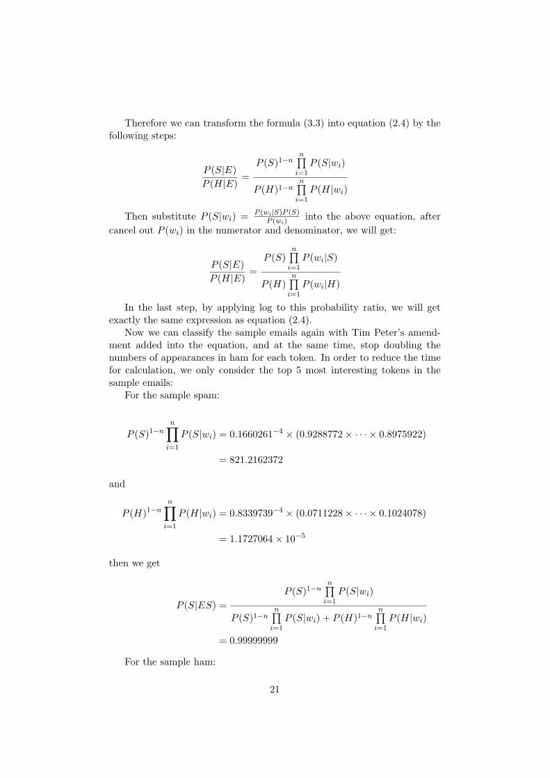
Therefore we can transform the formula (3.3) into equation (2.4) by thefollowing steps:

P (S|E)P (H|E)

=P (S)1−n

n∏i=1

P (S|wi)

P (H)1−nn∏

i=1P (H|wi)

Then substitute P (S|wi) = P (wi|S)P (S)P (wi)

into the above equation, aftercancel out P (wi) in the numerator and denominator, we will get:

P (S|E)P (H|E)

=P (S)

n∏i=1

P (wi|S)

P (H)n∏

i=1P (wi|H)

In the last step, by applying log to this probability ratio, we will getexactly the same expression as equation (2.4).

Now we can classify the sample emails again with Tim Peter’s amend-ment added into the equation, and at the same time, stop doubling thenumbers of appearances in ham for each token. In order to reduce the timefor calculation, we only consider the top 5 most interesting tokens in thesample emails:

For the sample spam:

P (S)1−nn∏

i=1

P (S|wi) = 0.1660261−4 × (0.9288772× · · · × 0.8975922)

= 821.2162372

and

P (H)1−nn∏

i=1

P (H|wi) = 0.8339739−4 × (0.0711228× · · · × 0.1024078)

= 1.1727064× 10−5

then we get

P (S|ES) =P (S)1−n

n∏i=1

P (S|wi)

P (S)1−nn∏

i=1P (S|wi) + P (H)1−n

n∏i=1

P (H|wi)

= 0.99999999

For the sample ham:

21

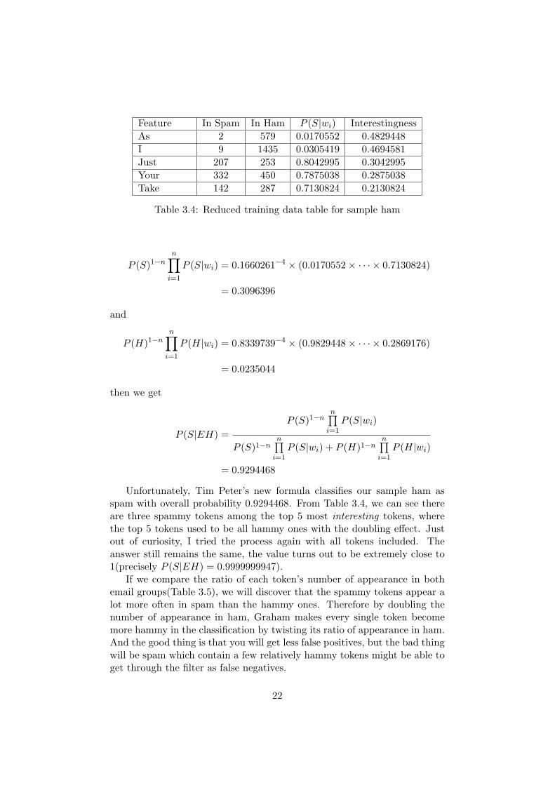
Feature In Spam In Ham P (S|wi) InterestingnessAs 2 579 0.0170552 0.4829448I 9 1435 0.0305419 0.4694581Just 207 253 0.8042995 0.3042995Your 332 450 0.7875038 0.2875038Take 142 287 0.7130824 0.2130824

Table 3.4: Reduced training data table for sample ham

P (S)1−nn∏

i=1

P (S|wi) = 0.1660261−4 × (0.0170552× · · · × 0.7130824)

= 0.3096396

and

P (H)1−nn∏

i=1

P (H|wi) = 0.8339739−4 × (0.9829448× · · · × 0.2869176)

= 0.0235044

then we get

P (S|EH) =P (S)1−n

n∏i=1

P (S|wi)

P (S)1−nn∏

i=1P (S|wi) + P (H)1−n

n∏i=1

P (H|wi)

= 0.9294468

Unfortunately, Tim Peter’s new formula classifies our sample ham asspam with overall probability 0.9294468. From Table 3.4, we can see thereare three spammy tokens among the top 5 most interesting tokens, wherethe top 5 tokens used to be all hammy ones with the doubling effect. Justout of curiosity, I tried the process again with all tokens included. Theanswer still remains the same, the value turns out to be extremely close to1(precisely P (S|EH) = 0.9999999947).

If we compare the ratio of each token’s number of appearance in bothemail groups(Table 3.5), we will discover that the spammy tokens appear alot more often in spam than the hammy ones. Therefore by doubling thenumber of appearance in ham, Graham makes every single token becomemore hammy in the classification by twisting its ratio of appearance in ham.And the good thing is that you will get less false positives, but the bad thingwill be spam which contain a few relatively hammy tokens might be able toget through the filter as false negatives.

22

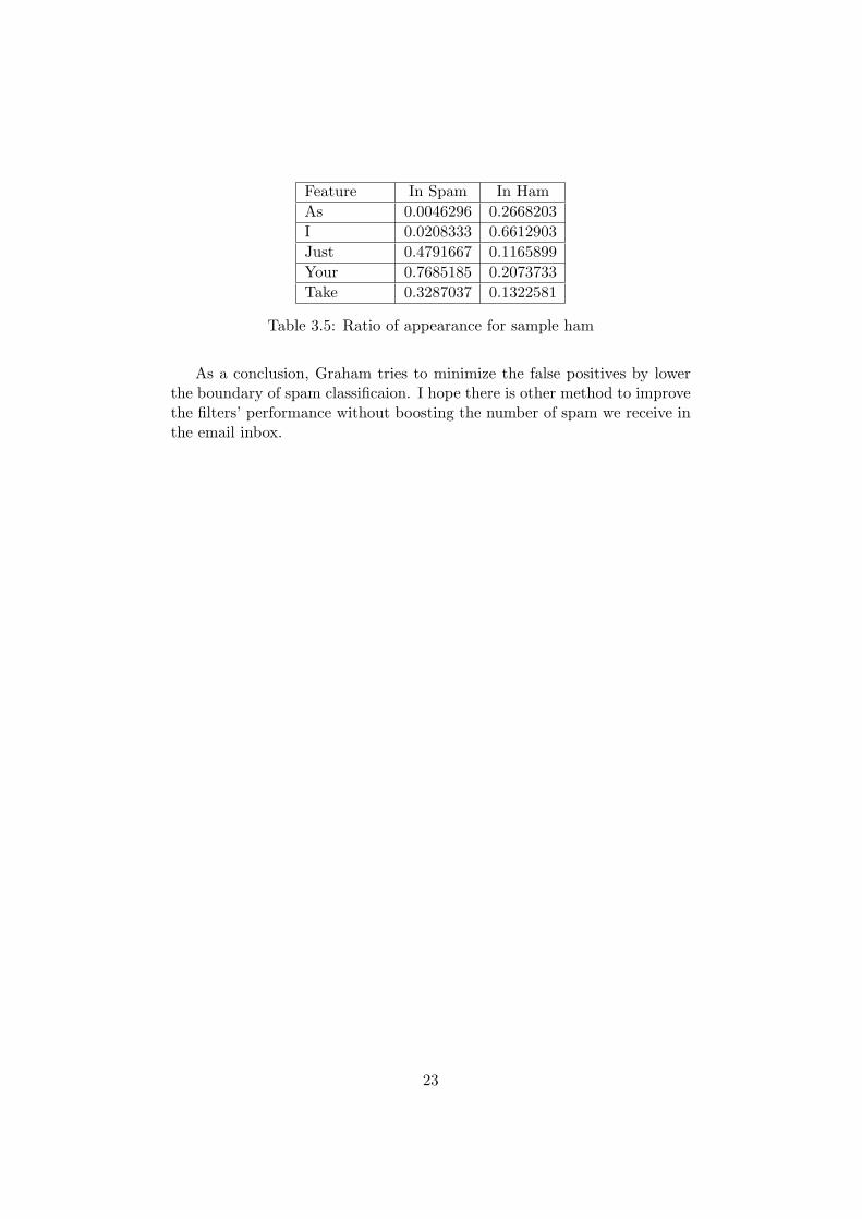
Feature In Spam In HamAs 0.0046296 0.2668203I 0.0208333 0.6612903Just 0.4791667 0.1165899Your 0.7685185 0.2073733Take 0.3287037 0.1322581

Table 3.5: Ratio of appearance for sample ham

As a conclusion, Graham tries to minimize the false positives by lowerthe boundary of spam classificaion. I hope there is other method to improvethe filters’ performance without boosting the number of spam we receive inthe email inbox.

23

Chapter 4

Unknown Tokens

4.1 Modified sample emails

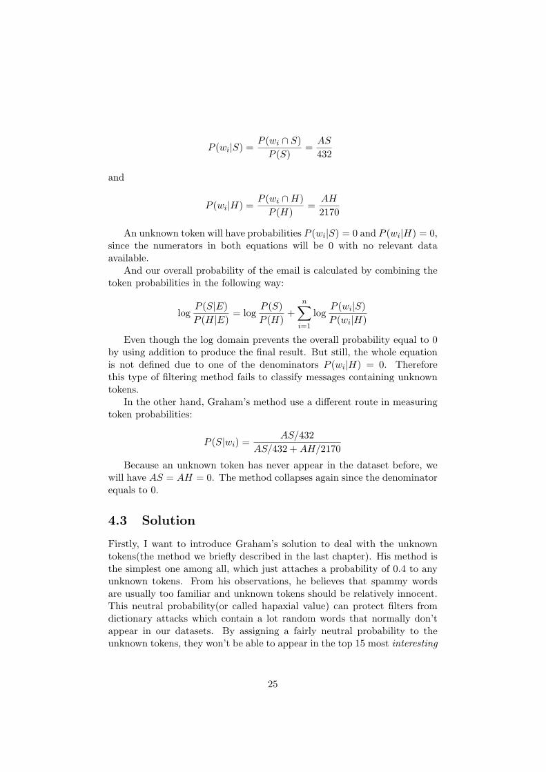
In order to investigate the consequence of containing an unknown token inthe email, I add one extra word into each of the sample emails we had earlier.Word great is added into the sample spam and word do is added into thesample ham, now the messages become:

• Example for spam with one extra word:

Paying too much for VIAGRA?

Now,you have a great chance to receive a FREE TRIAL!

• Example for ham with one extra word:

For the Clarins, just take your time. As i have advised her to doexercise regularly.

And of course, these two extra words are not included in my trainingdataset. The filters will therefore consider them as unknown tokens in theclassification later.

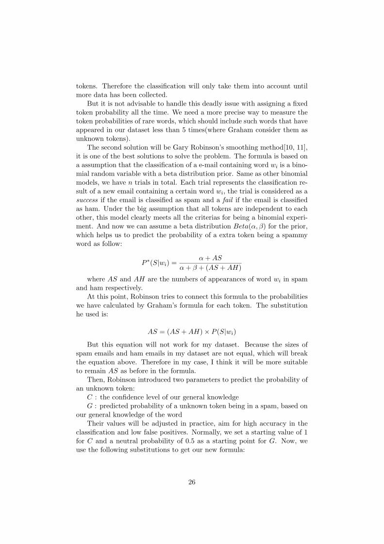
4.2 Problem

These tokens will cause a failure to the entire naive Bayes filtering process.The key factor here is that the overall probability of a email is a product ofall the individual token probabilities, one of them becomes 0 will result inthe overall probability equal to 0. Let’s review the previous two naive Bayesfiltering methods one by one to give us a better understanding of what hasgone wrong.

In the naive Bayes classification, we calculate token probabilities as fol-low, where AS and AH are the number of appearances of each token inspam and ham email groups respectively:

24

P (wi|S) =P (wi ∩ S)P (S)

=AS

432

and

P (wi|H) =P (wi ∩H)P (H)

=AH

2170

An unknown token will have probabilities P (wi|S) = 0 and P (wi|H) = 0,since the numerators in both equations will be 0 with no relevant dataavailable.

And our overall probability of the email is calculated by combining thetoken probabilities in the following way:

logP (S|E)P (H|E)

= logP (S)P (H)

+n∑

i=1

logP (wi|S)P (wi|H)

Even though the log domain prevents the overall probability equal to 0by using addition to produce the final result. But still, the whole equationis not defined due to one of the denominators P (wi|H) = 0. Thereforethis type of filtering method fails to classify messages containing unknowntokens.

In the other hand, Graham’s method use a different route in measuringtoken probabilities:

P (S|wi) =AS/432

AS/432 +AH/2170

Because an unknown token has never appear in the dataset before, wewill have AS = AH = 0. The method collapses again since the denominatorequals to 0.

4.3 Solution

Firstly, I want to introduce Graham’s solution to deal with the unknowntokens(the method we briefly described in the last chapter). His method isthe simplest one among all, which just attaches a probability of 0.4 to anyunknown tokens. From his observations, he believes that spammy wordsare usually too familiar and unknown tokens should be relatively innocent.This neutral probability(or called hapaxial value) can protect filters fromdictionary attacks which contain a lot random words that normally don’tappear in our datasets. By assigning a fairly neutral probability to theunknown tokens, they won’t be able to appear in the top 15 most interesting

25

tokens. Therefore the classification will only take them into account untilmore data has been collected.

But it is not advisable to handle this deadly issue with assigning a fixedtoken probability all the time. We need a more precise way to measure thetoken probabilities of rare words, which should include such words that haveappeared in our dataset less than 5 times(where Graham consider them asunknown tokens).

The second solution will be Gary Robinson’s smoothing method[10, 11],it is one of the best solutions to solve the problem. The formula is based ona assumption that the classification of a e-mail containing word wi is a bino-mial random variable with a beta distribution prior. Same as other binomialmodels, we have n trials in total. Each trial represents the classification re-sult of a new email containing a certain word wi, the trial is considered as asuccess if the email is classified as spam and a fail if the email is classifiedas ham. Under the big assumption that all tokens are independent to eachother, this model clearly meets all the criterias for being a binomial experi-ment. And now we can assume a beta distribution Beta(α, β) for the prior,which helps us to predict the probability of a extra token being a spammyword as follow:

P ∗(S|wi) =α+AS

α+ β + (AS +AH)

where AS and AH are the numbers of appearances of word wi in spamand ham respectively.

At this point, Robinson tries to connect this formula to the probabilitieswe have calculated by Graham’s formula for each token. The substitutionhe used is:

AS = (AS +AH)× P (S|wi)

But this equation will not work for my dataset. Because the sizes ofspam emails and ham emails in my dataset are not equal, which will breakthe equation above. Therefore in my case, I think it will be more suitableto remain AS as before in the formula.

Then, Robinson introduced two parameters to predict the probability ofan unknown token:

C : the confidence level of our general knowledgeG : predicted probability of a unknown token being in a spam, based on

our general knowledge of the wordTheir values will be adjusted in practice, aim for high accuracy in the

classification and low false positives. Normally, we set a starting value of 1for C and a neutral probability of 0.5 as a starting point for G. Now, weuse the following substitutions to get our new formula:

26

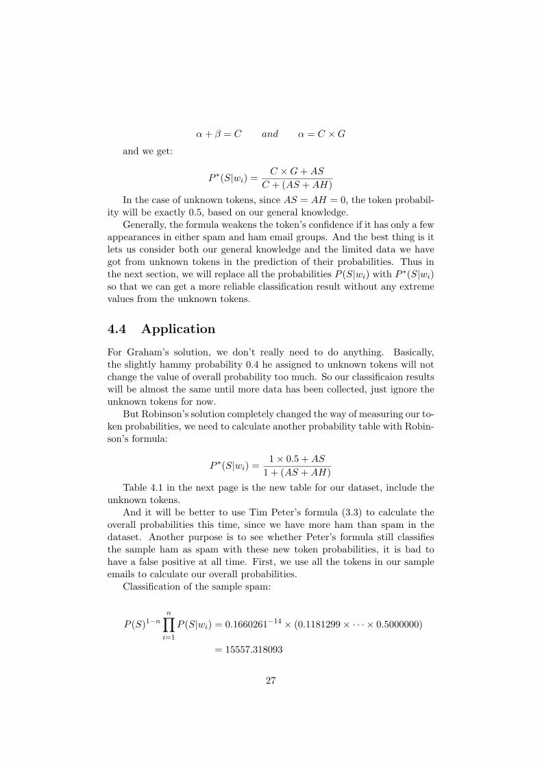
α+ β = C and α = C ×G

and we get:

P ∗(S|wi) =C ×G+AS

C + (AS +AH)

In the case of unknown tokens, since AS = AH = 0, the token probabil-ity will be exactly 0.5, based on our general knowledge.

Generally, the formula weakens the token’s confidence if it has only a fewappearances in either spam and ham email groups. And the best thing is itlets us consider both our general knowledge and the limited data we havegot from unknown tokens in the prediction of their probabilities. Thus inthe next section, we will replace all the probabilities P (S|wi) with P ∗(S|wi)so that we can get a more reliable classification result without any extremevalues from the unknown tokens.

4.4 Application

For Graham’s solution, we don’t really need to do anything. Basically,the slightly hammy probability 0.4 he assigned to unknown tokens will notchange the value of overall probability too much. So our classificaion resultswill be almost the same until more data has been collected, just ignore theunknown tokens for now.

But Robinson’s solution completely changed the way of measuring our to-ken probabilities, we need to calculate another probability table with Robin-son’s formula:

P ∗(S|wi) =1× 0.5 +AS

1 + (AS +AH)

Table 4.1 in the next page is the new table for our dataset, include theunknown tokens.

And it will be better to use Tim Peter’s formula (3.3) to calculate theoverall probabilities this time, since we have more ham than spam in thedataset. Another purpose is to see whether Peter’s formula still classifiesthe sample ham as spam with these new token probabilities, it is bad tohave a false positive at all time. First, we use all the tokens in our sampleemails to calculate our overall probabilities.

Classification of the sample spam:

P (S)1−nn∏

i=1

P (S|wi) = 0.1660261−14 × (0.1181299× · · · × 0.5000000)

= 15557.318093

27

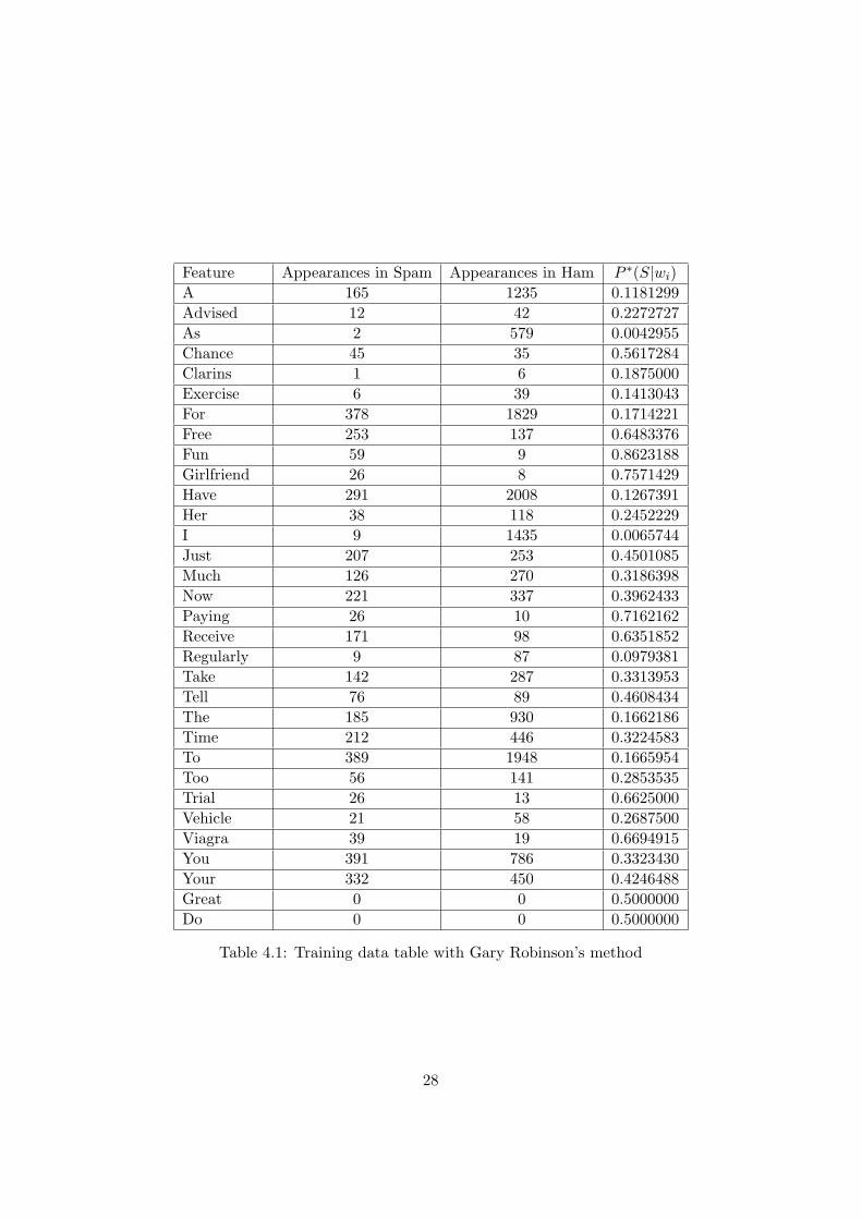
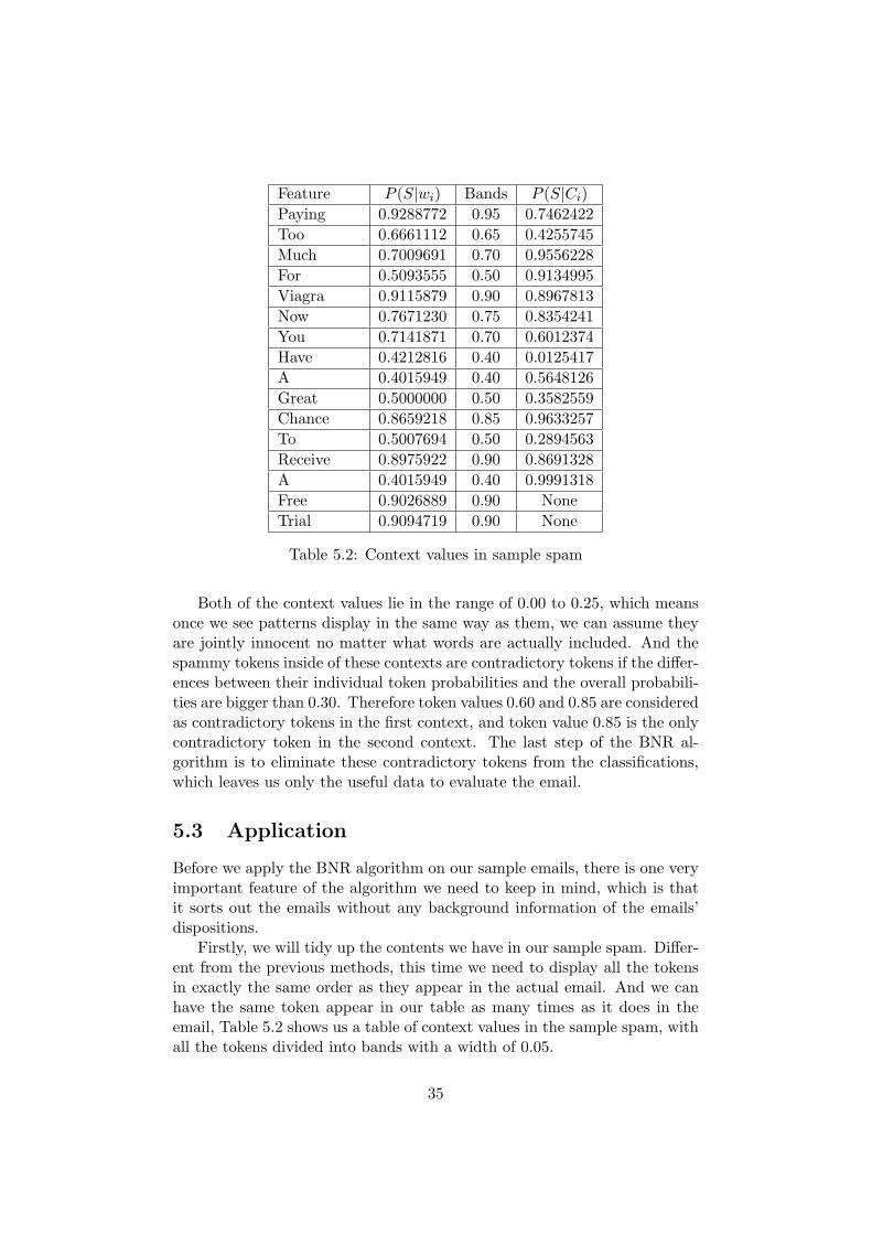
Feature Appearances in Spam Appearances in Ham P ∗(S|wi)A 165 1235 0.1181299Advised 12 42 0.2272727As 2 579 0.0042955Chance 45 35 0.5617284Clarins 1 6 0.1875000Exercise 6 39 0.1413043For 378 1829 0.1714221Free 253 137 0.6483376Fun 59 9 0.8623188Girlfriend 26 8 0.7571429Have 291 2008 0.1267391Her 38 118 0.2452229I 9 1435 0.0065744Just 207 253 0.4501085Much 126 270 0.3186398Now 221 337 0.3962433Paying 26 10 0.7162162Receive 171 98 0.6351852Regularly 9 87 0.0979381Take 142 287 0.3313953Tell 76 89 0.4608434The 185 930 0.1662186Time 212 446 0.3224583To 389 1948 0.1665954Too 56 141 0.2853535Trial 26 13 0.6625000Vehicle 21 58 0.2687500Viagra 39 19 0.6694915You 391 786 0.3323430Your 332 450 0.4246488Great 0 0 0.5000000Do 0 0 0.5000000

Table 4.1: Training data table with Gary Robinson’s method

28

and

P (H)1−nn∏

i=1

P (H|wi) = 0.8339739−14 × (0.8818701× · · · × 0.5000000)

= 0.001179893

then we get

P (S|ES) =P (S)1−n

n∏i=1

P (S|wi)

P (S)1−nn∏

i=1P (S|wi) + P (H)1−n

n∏i=1

P (H|wi)

= 0.999999924

Classification of the sample ham:

P (S)1−nn∏

i=1

P (S|wi) = 0.1660261−15 × (0.2272727× · · · × 0.5000000)

= 0.01249972

and

P (H)1−nn∏

i=1

P (H|wi) = 0.8339739−15 × (0.7727273× · · · × 0.5000000)

= 0.1992480

then we get

P (S|EH) =P (S)1−n

n∏i=1

P (S|wi)

P (S)1−nn∏

i=1P (S|wi) + P (H)1−n

n∏i=1

P (H|wi)

= 0.059031178

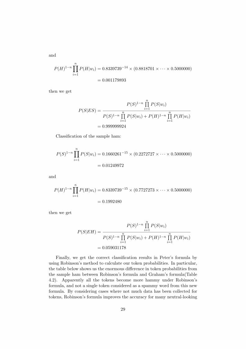
Finally, we get the correct classification results in Peter’s formula byusing Robinson’s method to calculate our token probabilities. In particular,the table below shows us the enormous difference in token probabilities fromthe sample ham between Robinson’s formula and Graham’s formula(Table4.2). Apparently all the tokens become more hammy under Robinson’sformula, and not a single token considered as a spammy word from this newformula. By considering cases where not much data has been collected fortokens, Robinson’s formula improves the accuracy for many neutral-looking

29

Feature In Spam In Ham P ∗(S|wi) P (S|wi)Advised 12 42 0.2272727 0.5893536As 2 579 0.0042955 0.0170552Clarins 1 6 0.1875000 0.4556909Exercise 6 39 0.1413043 0.4359180For 378 1829 0.1714221 0.5093555Have 291 2008 0.1267391 0.4212816Her 38 118 0.2452229 0.6179742I 9 1435 0.0065744 0.0305419Just 207 253 0.4501085 0.8042995Regularly 9 87 0.0979381 0.3419477Take 142 287 0.3313953 0.7130824The 185 930 0.1662186 0.4998070Time 212 446 0.3224583 0.7048131To 389 1948 0.1665954 0.5007694Your 332 450 0.4246488 0.7875038Do 0 0 0.5000000 0.4000000

Table 4.2: Comparison table of token probabilities in sample ham

Feature In Spam In Ham P ∗(S|wi) InterestingnessA 165 1235 0.1181299 0.3818701Have 291 2008 0.1267391 0.3732609To 389 1948 0.1665954 0.3334046For 378 1829 0.1714221 0.3285779Paying 26 10 0.7162162 0.2162162

Table 4.3: New ordered training data table for sample spam

emails. It successfully classified our sample ham as a legitimate email thistime, which reduced the number of false positives.

Next, we consider only the top 5 most interesting tokens in the calcula-tion. Let’s have a table of these tokens for each sample email first. (Table4.3 and Table 4.4)

Surprisingly, the top 4 most interesting tokens in the table for samplespam are all hammy words based on the token probabilities. This makes itdifficult for the formula to classify the message correctly with this misleadinginformation.

The new overall probabilities of the sample emails are calculated as fol-low:

Classification of the sample spam:

30

Feature In Spam In Ham P ∗(S|wi) InterestingnessAs 2 579 0.0042955 0.4957045I 9 1435 0.0065744 0.4934256Regularly 9 87 0.0979381 0.4020619Have 291 2008 0.1267391 0.3732609Exercise 6 39 0.1413043 0.3586957

Table 4.4: New ordered training data table for sample ham

P (S)1−nn∏

i=1

P (S|wi) = 0.1660261−4 × (0.1181299× · · · × 0.7162162)

= 0.4030312

and

P (H)1−nn∏

i=1

P (H|wi) = 0.8339739−4 × (0.8818701× · · · × 0.2837838)

= 0.3119720

then we get

P (S|ES) =P (S)1−n

n∏i=1

P (S|wi)

P (S)1−nn∏

i=1P (S|wi) + P (H)1−n

n∏i=1

P (H|wi)

= 0.5636775

Classification of the sample ham:

P (S)1−nn∏

i=1

P (S|wi) = 0.1660261−4 × (0.0042955× · · · × 0.1413043)

= 0.0000652

and

P (H)1−nn∏

i=1

P (H|wi) = 0.8339739−4 × (0.9957045× · · · × 0.8586957)

= 1.3831702

31

then we get

P (S|EH) =P (S)1−n

n∏i=1

P (S|wi)

P (S)1−nn∏

i=1P (S|wi) + P (H)1−n

n∏i=1

P (H|wi)

= 0.000047129

With a slightly spammy result from the classification of the sample spam,we can still identify the message as a spam. The reason will be that the num-ber of ham in our dataset is roughly five times the amount of spam we havegot. This factor reduces the effect of hammy words in the classification andgive more attention to the spammy ones. We also classify the sample ham asa legitimate email with no doubt. In conclusion, Robinson’s formula solvesthe problem of unknown tokens smoothly and generates a more accurateclassification for emails containing rare words.

32

Chapter 5

Bayesian Noise Reduction

5.1 Introduction

This chapter we are going to look at one of the major improvements inBayesian spam filtering, particularly useful in making the filtering processmore effective and gain more confidence in the classification. Jonathan A.Zdziarski first discussed about the Bayesian noise reduction algorithm in2004[15], and also include this idea in his book later[16, p. 231].

The noise we are talking about here is defined as words inconsistentwith the disposition of the pattern they belong to and can possibly lead toa misclassification of the message if not removed. Generally, the noise wereceive can be divided into two different groups. One group is the noise indaily chatting, it can be one of user’s close friends discuss about girls or anyspammy topics in a email which should indeed be classified as ham. Theother group will be the noise in spam, which normally is a bunch of randomwords with innocent token probabilities. They are added by the spammersin an attempt to flood filters with misleading information. But by applyingthe BNR algorithm before the classification, our filters will get a clearerdisplay of the messages’ original disposition and have a higher confidencelevel in decision making.

5.2 Zdziarski’s BNR algorithm

The Bayesian noise reduction algorithm consists of three stages: patterncontexts learning, identifying interesting contexts and detecting anomaliesin the contexts. In stage one, we sort out all the tokens into a set of patternswhich contains three consecutive tokens each(the size of pattern may vary,normally a window size of 3 is used in the algorithm). In stage two, value ofthe contexts will be measured and only the most interesting contexts will beconsidered into the next stage. In the final stage, we detect the statisticalanomalies in the contexts we get from the previous stage and eliminate them

33

Token P (S|wi) BandAdvised 0.59 0.60Chance 0.87 0.85I 0.03 0.05Regularly 0.34 0.35

Table 5.1: Pattern examples

from the classification.Before we can analyse the contexts, each token value will be assigned to

a band with width 0.05. We try to reduce the number of patterns need tobe identified in our dataset by doing this. For instance, some of the tokensfrom our dataset will fall into the bands shown at Table 5.1.

With a window size of 3, the following patterns will be created from thetokens above:

0.60 0.85 0.05 0.85 0.05 0.35

In practice, we will need to create such patterns for all the words in theemail we receive. A series of these patterns is called artificial contexts, andthey will be treated as individual tokens in the calculation later. Then wecalculate a probability for each pattern by using Graham’s method, but wedo not bias the number of appearances in ham for the BNR algorithm. Thusthe probability of pattern is calculated as follow:

P (S|Ci) =AS/432

AS/432 +AH/2170(5.1)

where in the equation above, AS is the number of appearance of thecontext Ci in spam and similarly AH represents the number of appearancein ham. We will also apply Robinson’s formula in calculating unknowntokens’ probabilities, in this case, both of our unknown tokens will have atoken probability of 0.5 and fall into the band 0.50.

Once we have all the context values, the next step is to find the mostinteresting contexts. This time we require not only the context’s valueneed to be at the two ends(close to 0 or 1), but also contains at least onecontradictory token. In order to be a interesting context in most Bayesianfilters, its value need to be in the range of either 0.00 to 0.25 or 0.75 to1.00. And the context must include at least one token with a relatively bigdifference between its probability and the overall probability of the pattern,normally a threshold of 0.30 will be suitable for the difference.

For the two patterns we created above, the pattern probabilities calcu-lated by equation (5.1) is the following:

0.60 0.85 0.05 [0.0260111] 0.85 0.05 0.35 [0.0956177]

34

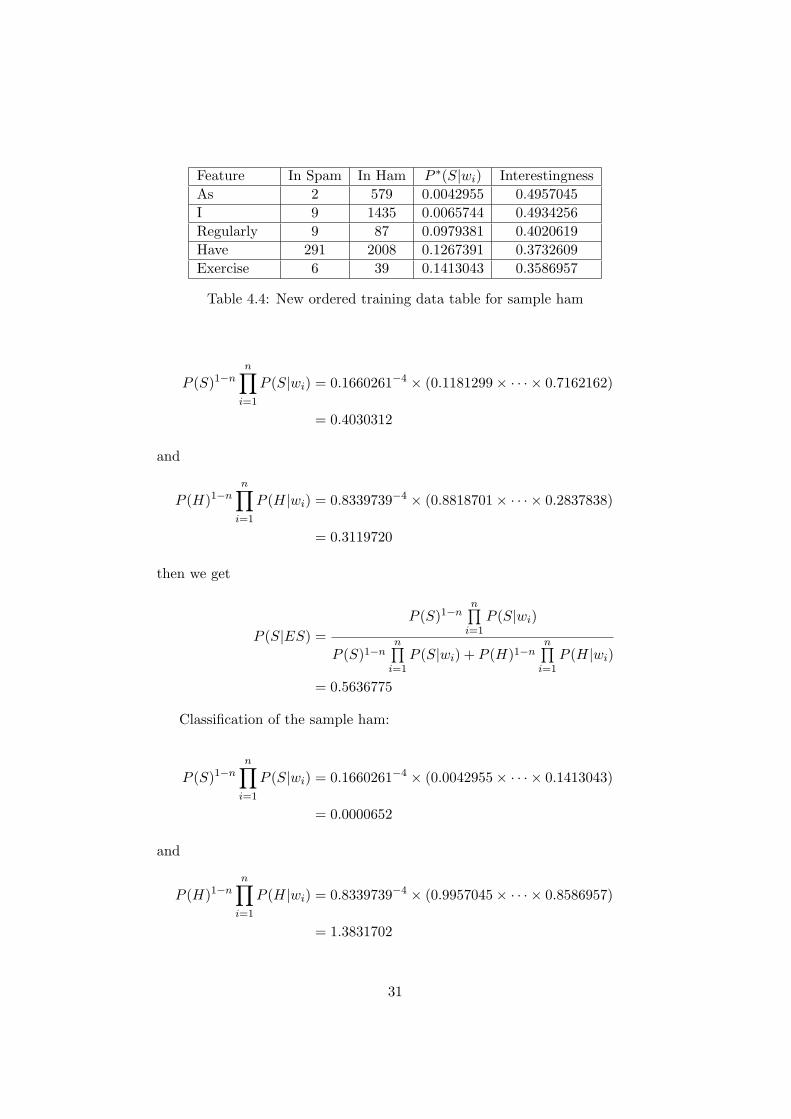
Feature P (S|wi) Bands P (S|Ci)Paying 0.9288772 0.95 0.7462422Too 0.6661112 0.65 0.4255745Much 0.7009691 0.70 0.9556228For 0.5093555 0.50 0.9134995Viagra 0.9115879 0.90 0.8967813Now 0.7671230 0.75 0.8354241You 0.7141871 0.70 0.6012374Have 0.4212816 0.40 0.0125417A 0.4015949 0.40 0.5648126Great 0.5000000 0.50 0.3582559Chance 0.8659218 0.85 0.9633257To 0.5007694 0.50 0.2894563Receive 0.8975922 0.90 0.8691328A 0.4015949 0.40 0.9991318Free 0.9026889 0.90 NoneTrial 0.9094719 0.90 None

Table 5.2: Context values in sample spam

Both of the context values lie in the range of 0.00 to 0.25, which meansonce we see patterns display in the same way as them, we can assume theyare jointly innocent no matter what words are actually included. And thespammy tokens inside of these contexts are contradictory tokens if the differ-ences between their individual token probabilities and the overall probabili-ties are bigger than 0.30. Therefore token values 0.60 and 0.85 are consideredas contradictory tokens in the first context, and token value 0.85 is the onlycontradictory token in the second context. The last step of the BNR al-gorithm is to eliminate these contradictory tokens from the classifications,which leaves us only the useful data to evaluate the email.

5.3 Application

Before we apply the BNR algorithm on our sample emails, there is one veryimportant feature of the algorithm we need to keep in mind, which is thatit sorts out the emails without any background information of the emails’dispositions.

Firstly, we will tidy up the contents we have in our sample spam. Differ-ent from the previous methods, this time we need to display all the tokensin exactly the same order as they appear in the actual email. And we canhave the same token appear in our table as many times as it does in theemail, Table 5.2 shows us a table of context values in the sample spam, withall the tokens divided into bands with a width of 0.05.

35

Based on this table, we identify all the interesting patterns and findout the contradictory tokens in them. For the sample spam, we decide toeliminate the following tokens:

For Have A Great To A

0.50 0.40 0.40 0.50 0.50 0.40

Thus, only the following tokens will be considered in the classification:

Paying Too Much Viagra Now You Chance Receive Free Trial

0.95 0.65 0.70 0.90 0.75 0.70 0.85 0.90 0.90 0.90

As you can see, the noise we removed from the email are the tokenswith neutral probabilities. Now we can classify the sample spam easily withpurely spammy tokens within the email. By using Tim Peter’s formula (3.3),we get a overall probability of 1.0000000 for the sample spam(the value isnot actually equal to 1, but extremely close to). This will be a ideal casefor applying the BNR algorithm to prevent innocent word attacks from thespammers.

Next, we will apply the BNR algorithm in the sample ham, which ismore important since reducing the number of false positives is crucial forall types of filters. Similarly, we will create a table of context values for thesample ham(Table 5.3).

The table of context values is quite different this time, half of the patternprobabilities are less than 0.6. Therefore the dispositions of our patternsfrom this sample email are relatively hammy, which is consistent to thecharacter of a ham. And also we have less interesting patterns but one morecontradictory tokens in the sample ham, the eliminations is as follow:

Clarins Just As I Have Advised Her

0.45 0.80 0.00 0.05 0.40 0.60 0.60

And the remaining tokens is the following:

For The Take Your Time To Do Exercise Regularly

0.50 0.50 0.70 0.80 0.70 0.50 0.50 0.45 0.35

Even three relatively spammy tokens have been removed from the classi-fication, the overall probability of the sample ham still indicates the email asa spam with a very spammy value(0.9999997) under Peter’s method. In thiscase, I decide to enlarge the window size of patterns. Instead of a window

36

Feature P (S|wi) Bands P (S|Ci)For 0.5093555 0.50 0.3699153The 0.4998070 0.50 0.2298456Clarins 0.4556909 0.45 0.8231455Just 0.8042995 0.80 0.6542389Take 0.7130824 0.70 0.7543587Your 0.7875038 0.80 0.9723396Time 0.7048131 0.70 0.9128645As 0.0170552 0.00 0.9988764I 0.0305419 0.05 0.3207863Have 0.4212816 0.40 0.7324567Advised 0.5893536 0.60 0.2378975Her 0.6179742 0.60 0.5156789To 0.5007694 0.50 0.5982764Do 0.5000000 0.50 0.2180439Exercise 0.4359180 0.45 NoneRegularly 0.3419477 0.35 None

Table 5.3: Context values in sample ham

Feature P (S|wi) Bands P (S|Ci)For 0.5093555 0.50 0.8965467The 0.4998070 0.50 0.8145563Clarins 0.4556909 0.45 0.9543357Just 0.8042995 0.80 0.7043126Take 0.7130824 0.70 0.2398641Your 0.7875038 0.80 0.1974217Time 0.7048131 0.70 0.1746881As 0.0170552 0.00 0.7169663I 0.0305419 0.05 0.0965754Have 0.4212816 0.40 0.5524785Advised 0.5893536 0.60 0.6519348Her 0.6179742 0.60 0.4145956To 0.5007694 0.50 NoneDo 0.5000000 0.50 NoneExercise 0.4359180 0.45 NoneRegularly 0.3419477 0.35 None

Table 5.4: New context values in sample ham

37

size of 3, we will create a new table of context values for the sample hamwith a window size of 5(Table 5.4).

Surprisingly, with the same number of interesting patterns(7 patterns,same as the previous case with a window size of 3), we have 10 contradictorytokens under the new criteria for patterns.

Contradictory tokens:

For The Clarins Take Your Time Have Advised Her To

0.50 0.50 0.45 0.70 0.80 0.70 0.40 0.60 0.60 0.50

And we have the following tokens left for classification:

Just As I Do Exercise Regularly

0.80 0.00 0.05 0.50 0.45 0.35

With only one spammy token in our classification, our overall proba-bility for the sample ham decreases to 0.7426067 by using Peter’s formula.Basically, the BNR algorithm will be able to perceive more inconsistenciesby expanding the window size of patterns and improve the accuracy of clas-sification.

Since our filter still classify the sample ham as a spam, I tried the BNRalgorithm again with a window size of 6 for the patterns. And two moretokens are eliminated as contradictory tokens, which are the following:

Just Do

0.80 0.50

These are the top 2 most spammy words in the remaining text we gotpreviously. Finally we have all hammy tokens in the classification, and theresult is very encouraging this time, a overall probability of 0.0270686 forthe sample ham. That means we managed to reduce the amount of falsepositives with bigger window size for the patterns, in a exchange of slightlyhigher false negative rates. This side effect should be acceptable for mostBayesian filters, because reducing the number of false positives is alwaystheir number one priority.

38

Chapter 6

Conclusion

The aim of this project is to demonstrate the high performance of a simplestatistical filtering method: naive Bayes classification.

The project starts with a introduction of the basic naive Bayes classifi-cation in Chapter 2, working along with our two sample emails as trainingdata. The filtering process was quite straightforward, and by applying thelog into the equation overcomes the problem of extremely small value fromthe products. And the application in the end showed that the naive Bayesclassification successfully classified the two sample emails into the correctemail groups.

In Chapter 3, we introduced Paul Graham’s way of implementing thenaive Bayes classification on spam filtering. In Graham’s method, he decidesto calculate the probabilities P (S|wi) and P (H|wi) for each token instead ofprobabilities P (wi|S) and P (wi|H) in the previous chapter. And he doublesthe number of appearance in ham for each token in order to reduce falsepositives in the classification. Another important feature of his method isthat he only consider the top 15 most interesting tokens in the classification.As the sample emails we had only have 15 tokens in each, I applied themethod on the sample emails again with only the top 5 most interestingtokens were considered. Not surprisingly, the results of the classificationwere still correct. But Graham’s method is created based on a dataset withequal amount of spam and ham, which is clearly not suitable for generalcases. Tim Peter’s adjustment for the method sorted out this problem, butunfortunately, his method failed to classify our sample ham correctly in theapplication later.

Chapter 4 discussed the problem of containing unknown tokens in ourclassification and the sample emails were modified for further testing. Twosolutions were introduced in this chapter, where Graham’s solution is simplyassign a neutral probability of 0.4 to all the unknown tokens and GaryRobinson’s smoothing method completely changed the way of calculating thetoken values. By considering cases where not much data has been collected

39

for tokens, Robinson’s formula improves the accuracy for many neutral-looking emails. It successfully classified our sample ham as a legitimateemail in the application later, which reduced the number of false positives.

The last chapter showed us one of the major improvements in Bayesianspam filtering: Bayesian noise reduction. The BNR algorithm was demon-strated in three stages, pattern contexts learning, identifying interestingcontexts and detecting anomalies in the contexts. And we managed to clas-sify our sample emails more effectively in the application section.

But still, there are many other ways of implementing the naive Bayesclassification haven’t been discussed in this project. Such as Multi-variateBernoulli naive Bayes classifier[14, 6], Multinomial naive Bayes classifier[4]and Poisson naive Bayes classifier[13]. All of them have great improvementsbased on the basic naive Bayes classification and works particularly wellunder different circumstances. Spam filtering is a race between spammersand spam filtering programmers, study and research in this field will neverstop as long as the spam still appears in our email inbox.

AcknowledgementI want to give many thanks to my project supervisor, Matthias Trof-

faes. For his superb guidance throughout my project and lots of decentsuggestions during the final stage of this project.

40

Bibliography

[1] Vasanth Elavarasan and Mohamed Gouda. Email filters that usespammy words only, May 2006.

[2] Paul Graham. A plan for spam. In Reprinted in Paul Graham, Hackersand Painters, Big Ideas from the Computer Age, O Really, 2004, 2002.

[3] Konstantinos V. Chandrinos George Paliouras Ion Androutsopoulos,John Koutsias and Constantine D. Spyropoulos. An evaluation of naivebayesian anti-spam filtering. In Workshop on Machine Learning in theNew Information Age, pages 9–17, Jun 2000.

[4] J. Teevan J. Rennie, L. Shih and D. Karger. Tackling the poor assump-tions of naive bayes text classifiers. In ICML, 2003.

[5] David D. Lewis. Naive (bayes) at forty: The independence assumptionin information retrieval. In Proceedings of ECML-98, 10th EuropeanConference on Machine Learning, number 1398, pages 4–15. SpringerVerlag, Heidelberg, DE, 1998.

[6] A. Mccallum and K. Nigam. A comparison of event models for naivebayes text classification, 1998.

[7] Tim Peter, August 2002. http://mail.python.org/pipermail/python-dev/2002-August/028216.html.

[8] Prabhakar Raghavan and Christopher Manning. Text classification:The naive bayes algorithm, 2003.

[9] Peter E. Hart Richard O. Duda and David G. Stork. Pattern Classifi-cation (2nd Edition). Wiley-Interscience, November 2000.

[10] Gary Robinson. A statistical approach to the spam problem. Linux J.,2003(107), March 2003.

[11] Gary Robinson. Spam detection, January 2006.

[12] Mehran Sahami, Susan Dumais, David Heckerman, and Eric Horvitz.A bayesian approach to filtering junk e-mail. In Learning for Text

41

Categorization: Papers from the 1998 Workshop, Madison, Wisconsin,1998. AAAI Technical Report WS-98-05.

[13] Hee C. Seo Sang B. Kim and Hae C. Rim. Poisson naive bayes fortext classification with feature weighting. In Proceedings of the sixthinternational workshop on Information retrieval with Asian languages,pages 33–40, Morristown, NJ, USA, 2003. Association for Computa-tional Linguistics.

[14] Ion Androutsopoulos Vangelis Metsis and Georgios Paliouras. Spamfiltering with naive bayes - which naive bayes?, 2006.

[15] Jonathan A. Zdziarski. Bayesian noise reduction:contextual symmetrylogic utilizing pattern consistency analysis, December 2004.

[16] Jonathan A. Zdziarski. Ending spam:Bayesian content filtering and theart of statistical language classification. No Starch Press, San Francisco,2005.

42