SPACETIME CALCULUS for GRAVITATION THEORY

David HestenesArizona State University

Abstract

A new gauge theory of gravitation on flat spacetime has recently been

developed by Lasenby, Doran, and Gull in the language of Geometric

Calculus. This paper provides a systematic account of the mathemati-

cal formalism to facilitate applications and extensions of the theory. It

includes formulations of differential geometry, Lie derivatives and inte-

grability theorems which are coordinate-free and gauge-covariant. Em-

phasis is on use of the language to express physical and geometrical

concepts.

CONTENTS

Part I. Mathematical Fundamentals

1. Spacetime Algebra2. Vector Derivatives and Differentials3. Linear Algebra4. Tensors and their Classification5. Transformations on Spacetime6. Directed Integrals and the Fundamental Theorem

Part II. Induced Geometry on Flat Spacetime

7. Gauge Tensor and Gauge Invariance8. Covariant Derivatives and Parallel Transport9. From Gauge to Connexion

10. Coderivatives and Integrals11. Curvature

Part III. Spacetime Flows

12. Gauge Covariant Flows and Flow Derivatives13. Integrability and Coordinates14. Flow Dynamics and Deformations

1996 PACS: 04.20.Cv, 11.15.-q, 02.40.-k, 11.30.Cp.

1

Introduction

Lasenby, Doran and Gull have recently created a powerful coordinate-free reformulation,refinement, and extension of general relativity [1,2]. It is a gauge theory on flat spacetime,but it retains the attractive geometric structure of Einstein’s theory. The mathematicalformalism which they employ comes mostly from [3], with additional pieces from [4-8]and elsewhere. It is not easy, however, to assimilate and adapt the formalism from thesereferences. Although much of that has already been done in [1], further discussion andanalysis will help make the whole approach more accessible. Also, the emphasis here ismore strongly focused on notions of differential geometry in formulating the theory. Indeed,the method amounts to a new approach to differential geometry which could fairly be calledgauge geometry.

The general mathematical formalism is called geometric calculus or, when it refers specif-ically to spacetime, spacetime calculus. This paper presents a systematic account of space-time calculus for the purposes of gravitation theory. It is divided into three parts.

Part I reviews the fundamentals of spacetime calculus with emphasis on those relevantto gravitation theory. Many of the proofs are omitted, since they can easily be supplied orfound in the references. Otherwise, the treatment is self-contained.

Part II develops gauge covariant Riemannian geometry on flat spacetime. The mainobjective is to clarify the fundamental ideas and provide a systematic account of the def-initions, theorems, proofs, and computational techniques needed to apply the spacetimecalculus efficiently to any physical problem. Specific physical applications are not ad-dressed here; excellent examples, which amply demonstrate the computational power ofthe calculus, have been worked out in [1,2] and [9–13].

Part III extends the spacetime calculus to deal systematically with congruences of curvesand associated concepts, such as Lie derivatives, Killing vectors and the theorem of Frobe-nius. The gauge covariant formulation of these concepts is a new idea with broad implica-tions for mathematics as well as physics. The treatment here is primarily a translation ofwell known concepts and results into the new formalism; proofs are consequently sketchy oromitted. (For comparison, a standard “modern” approach to the same topics can be foundin [14]). The translation is nontrivial and we concentrate here on consolidating the mainideas and results to facilitate applications. The main applications are likely to involve a“relativistically gauge covariant” continuum mechanics, including gravitational wave prop-agation. As a first step, a general definition and equation of motion for the deformationtensor is presented.

In a lengthy and profound analysis of the relation between physics and geometry, com-posed more than a decade before the advent of Einstein’s General Theory of Relativity(GR), Henri Poincare [15] concluded that: “One geometry cannot be more true than an-other; it can only be more convenient. Now, Euclidean geometry is and will remain, themost convenient.” After more analysis he added: “What we call a straight line in astronomyis simply the path of a ray of light. If, therefore, we were to discover negative parallaxes, orto prove that all parallaxes are higher than a certain limit, we should have a choice betweentwo conclusions: we could give up Euclidean geometry, or modify the laws of optics, andsuppose that light is not rigorously propagated in a straight line. It is needless to add thatevery one would look upon this solution as the more advantageous.” Applied to GR, thisamounts to the claim that any curved-space formulation of the theory can be replaced by

2

an equivalent and simpler flat-space formulation. Ironically, the curved-space formulationhas been preferred by nearly everyone since the inception of GR, and competing flat-spaceformulations certainly have not exhibited any of the simplicity anticipated by Poincare.One wonders if the trend might have been different if Poincare were still alive to promotehis view when GR made its spectacular appearance on the scene.

The situation has been changed dramatically by the new gauge formulation of GR [1,2].In retrospect, the popular “vierbein” approach to GR can be seen as a step toward aflat-space formulation, but it did not exhibit clear theoretical or practical simplificationsuntil it was expressed in the language of geometric calculus (GC) in [5]. The superior-ity of GC in practical calculations involving the curvature tensor was also demonstratedthere. By reinterpreting the GC formulation the new gauge theory has greatly clarifiedGR and produced numerou examples of computational simplifications. All this amounts tocompelling evidence that Poincare was right in the first place.

Part I. MATHEMATICAL FUNDAMENTALS

1. Spacetime Algebra

We represent Minkowski spacetime as a real 4-dimensional vector space M4. The twoproperties of scalar multiplication and vector addition in M4 provide only a partial spec-ification of spacetime geometry. To complete the specification we introduce an associativegeometric product among vectors a, b, c, . . . with the property that the square of any vectoris a (real) scalar. Thus for any vector a we can write

a2 = aa = ε| a |2 , (1.1)

where ε is the signature of a and | a | is a (real) positive scalar. As usual, we say that a istimelike, lightlike or spacelike if its signature is positive (ε = 1), null (ε = 0), or negative(ε = −1). To specify the signature of M4 as a whole, we adopt the axioms: (a) M4 containsat least one timelike vector; and (b) Every 2-plane in M4 contains at least one spacelikevector.

The vector space M4 is not closed under the geometric product just defined. Rather,by multiplication and (distributive) addition it generates a real, associative (but noncom-mutative), geometric algebra of dimension 24 = 16, called the spacetime algebra (STA).The name is appropriate because all the elements and operations of the algebra have ageometric interpretation, and it suffices for the representation of any geometric structureon spacetime.

From the geometric product ab of two vectors it is convenient to define two other products.The inner product a · b is defined by

a · b = 12 (ab + ba) = b · a , (1.2)

and the outer product a ∧ b is defined by

a ∧ b = 12 (ab − ba) = −b ∧ a . (1.3)

3

The three products are therefore related by the important identity

ab = a · b + a ∧ b , (1.4)

which can be seen as a decomposition of the product ab into symmetric and antisymmetricparts.

From (1.1) it follows that the inner product a · b is scalar-valued. The outer product a∧ bis neither scalar nor vector but a new entity called a bivector, which can be interpretedgeometrically as an oriented plane segment, just as a vector can be interpreted as an orientedline segment.

Inner and outer products can be generalized. The outer product and the notion of k-vector can be defined iteratively as follows: Scalars are regarded as 0-vectors, vectors as1-vectors and bivectors as 2-vectors. For a given k-vector K the positive integer k is calledthe grade (or step) of K. The outer product of a vector a with K is a (k +1)-vector definedin terms of the geometric product by

a ∧ K = 12 (aK + (−1)kKa) = (−1)kK ∧ a , (1.5)

The corresponding inner product is defined by

a · K = 12 (aK + (−1)k+1Ka) = (−1)k+1K · a, (1.6)

and it can be proved that the result is a (k − 1)-vector. Adding (1.5) and (1.6) we obtain

aK = a · K + a ∧ K , (1.7)

which obviously generalizes (1.4). The important thing about (1.7) is that it decomposesaK into (k − 1)-vector and (k + 1)-vector parts.

Manipulations and inferences involving inner and outer products are facilitated by a hostof theorems and identities given in [3] of which the most important are recorded here. Theouter product is associative, and

a1 ∧ a2 ∧ . . . ∧ ak = 0 (1.8)

if and only if the vectors a1, a2, . . . , ak are linearly dependent. Since M4 has dimension 4,(1.8) is an identity in STA for k > 4, so the generation of new elements by multiplicationwith vectors terminates at k = 4. A nonvanishing k-vector can be interpreted as a directedvolume element for Mk spanned by the vectors a1, a2, . . . , ak. In STA 4-vectors are calledpseudoscalars, and for any four such vectors we can write

a1 ∧ a2 ∧ a3 ∧ a4 = λi , (1.9)

where i is the unit pseudoscalar and λ is a scalar which vanishes if the vectors are linearlydependent.

The unit pseudoscalar is so important that the special symbol i is reserved for it. It hasthe properties

i2 = −1 , (1.10)

4

and for every vector a in M4

ia = −ai . (1.11)

Of course, i can be interpreted geometrically as the (unique) unit oriented volume elementfor spacetime. A convention for specifying its orientation is given below. Multiplicativeproperties of the unit pseudoscalar characterize the geometric concept of duality. The dualof a k-vector K in STA is the (4 − k)-vector defined (up to a sign) by iK or Ki. Trivially,every pseudoscalar is the dual of a scalar. Every 3-vector is the dual of a vector; for thisreason 3-vectors are often called pseudovectors. The inner and outer products are dualto one another. This is easily proved by using (1.7) to expand the associative identity(aK)i = a(Ki) in two ways:

(a · K + a ∧ K)i = a · (Ki) + a ∧ (Ki) .

Each side of this identity has parts of grade (4−k±1) and which can be separately equated,because they are linearly independent. Thus, one obtains the duality identities

(a · K)i = a ∧ (Ki) , (1.12a)

(a ∧ K)i = a · (Ki) , (1.12b)

Note that (1.12a) can be solved for

a · K = [a ∧ (Ki)]i−1 , (1.13)

which could be used to define the inner product from the outer product and duality.Unlike the outer product, the inner product is not associative. Instead, it obeys various

identities, of which the following involving vectors, k-vector K and s-vector B are mostimportant:

(b ∧ a) · K = b · (a · K) = (K · b) · a = K · (b ∧ a) for grade k ≥ 2 , (1.14)

a · (K ∧ B) = (a · K) ∧ B + (−1)kK ∧ (a · B) . (1.15)

The latter implies the following identity involving vectors alone:

a · (a1 ∧ a2 ∧ . . . ∧ ak) = (a · a1)a2 ∧ . . . ∧ ak − (a · a2)a1 ∧ a3 . . . ∧ ak+· · · + (−1)k−1(a · ak)a1 ∧ a2 . . . ∧ ak−1 . (1.16)

This is called the Laplace expansion, because it generalizes and implies the familiar expan-sion for determinants. The simplest case is used so often that it is worth writing down:

a · (b ∧ c) = (a · b)c − (a · c)b = a · b c − a · c b . (1.17)

Parentheses have been eliminated here by invoking a precedence convention, that in am-biguous algebraic expressions inner products are to be formed before outer products, andboth of those before geometric products. This convention allows us to drop parentheses onthe right side of (1.16) but not on the left.

5

The entire spacetime algebra is generated by taking linear combinations of k-vectorsobtained by outer multiplication of vectors in M4. A generic element of the STA is calleda multivector. Any multivector M can be written in the expanded form

M = α + a + F + bi + βi =4∑

k=0

〈M 〉k , (1.18)

where a and b are scalars, a and b are vectors and F is a bivector. This is a decompositionof M into its “k-vector parts” 〈M 〉k, where

〈M 〉0 = 〈M 〉 = α (1.19)

is the scalar part, 〈M 〉1 = a is the vector part, 〈M 〉2 = F is the bivector part, 〈M 〉3 = biis the pseudovector part and 〈M 〉4 = βi is the pseudoscalar part. Duality has been used tosimplify the form of the trivector part in (1.18) by expressing it as the dual of a vector. Likethe decomposition of a complex number into real and imaginary parts, the decomposition(1.18) is significant because the parts with different grade are linearly independent of oneanother and have distinct geometric interpretations. On the other hand, multivectors ofmixed grade often have geometric significance that transcends that of their graded parts.

Any multivector M can be uniquely decomposed into parts of even and odd grade as

M± = 12 (M ∓ iMi) . (1.20)

In terms of the expanded form (1.18), the even part can be written

M+ = α + F + βi , (1.21)

while the odd part becomesM− = a + bi . (1.22)

The set M+ of all even multivectors forms an important subalgebra of STA called theeven subalgebra. Spinors can be represented as elements of the even subalgebra.

Computations are facilitated by the operation of reversion, defined for arbitrary multi-vectors M and N by

(MN)˜ = NM , (1.23a)

witha = a (1.23b)

for any vector a. For M in the expanded form (1.18), the reverse M is given by

M = α + a − F − bi + βi . (1.24)

Note that bivectors and trivectors change sign under reversion while scalars and pseu-doscalars do not.

This mathematical apparatus makes it possible to formulate and solve fundamental equa-tions without using coordinates. Nevertheless, STA facilitates the manipulation of coordi-nates, as shown below and in later sections of this document. Let γµ;µ = 0, 1, 2, 3 be

6

a right-handed orthonormal frame of vectors in M4 with γ0 in the forward light cone. Inaccordance with (1.2), we can write

ηµν ≡ γµ · γν = 12 (γµγν + γνγµ) . (1.25)

This may be recognized as the defining condition for the “Dirac algebra,” which is a matrixrepresentation of STA over a complex number field instead of the reals. Although thepresent interpretation of the γµ as an orthonormal frame of vectors is quite differentfrom their usual interpretation as matrix componentsof a single vector, it can be shownthat these alternatives are in fact compatible.

The orientation of the unit pseudoscalar i relative to the frame γµ is set by the equation

i = γ0γ1γ2γ3 = γ0 ∧ γ1 ∧ γ2 ∧ γ3 . (1.26)

We shall refer to γµ as a standard frame, without necessarily associating it with thereference frame of a physical observer. For manipulating coordinates it is convenient tointroduce the reciprocal frame γµ defined by the equations

γµ = ηµνγν or γµ · γν = δνµ . (1.27)

(summation convention assumed). “Rectangular coordinates” xν of a spacetime point xare then given by

xν = γν · x and x = xνγν . (1.28)

The γµ generate by multiplication a complete basis for STA, consisting of the 24 = 16linearly independent elements

1, γµ, γµ ∧ γν , γµi, i . (1.29)

Any multivector can be expressed as a linear combination of these elements. For example,a bivector F has the expansion

F = 12Fµνγµ ∧ γν , (1.30)

with its “scalar components” given by

Fµν = γµ · F · γν = γν · (γµ · F ) = (γν ∧ γµ) · F . (1.31)

However, such an expansion is seldom needed.Besides the inner and outer products defined above, many other products can be defined

in terms of the geometric product. The commutator product A × B is defined for any Aand B by

A × B ≡ 12 (AB − BA) = −B × A . (1.32)

Mathematicians classify this product as a “derivation” with respect to the geometric product,because it has the “distributive property”

A × (BC) = (A × B)C + B(A × C) . (1.33)

7

This implies the Jacobi Identity

A × (B × C) = (A × B) × C + B × (A × C) , (1.34)

which is a derivation on the commutator product. The relation of the commutator productto the inner and outer products is grade dependent; thus, for a vector a,

a × 〈M 〉k = a ∧ 〈M 〉k if k is odd , (1.35a)

a × 〈M 〉k = a · 〈M 〉k if k is even . (1.35b)

The commutator product is especially useful in computations with bivectors. With anybivector A this product is grade preserving:

A × 〈M 〉k = 〈A × M 〉k . (1.36)

In particular, this implies that the space of bivectors is closed under the commutatorproduct. It therefore forms a Lie algebra — which is, in fact, the Lie algebra of the Lorentzgroup. The geometric product of bivector A with M has the expanded form

AM = A · M + A × M + A ∧ M for grade M ≥ 2 . (1.37)

This should be compared with the corresponding expansion (1.4) for the product of vectors.For any bivector F , (1.37) assures us that we can write

F 2 = F · F + F ∧ F = | f |2ei2ϕ .

When F 2 = 0, this can be solved for the “invariant angle ϕ,” given by

i tan 2ϕ =F ∧ F

F · F. (1.38)

Then F can be written in the canonical form

F = feiϕ . (1.39)

When F 2 = 0, F can still be written in the form (1.39) with

f = k ∧ e = ke , (1.40)

where k is a null vector and e is spacelike. In this case, the decomposition is not unique,and the exponential factor can always be absorbed in the definition of f . The canonicalbivector decomposition (1.39) is especially useful in treating the electromagnetic field.

2. Vector Derivatives and Differentials

To extend spacetime algebra into a complete spacetime calculus, suitable definitions forderivatives and integrals are required. In terms of the coordinates (1.28), an operator∇ ≡ ∂x interpreted as the derivative with respect to a spacetime point x can be defined by

∇ = γµ∂µ (2.1)

8

where∂µ =

∂

∂xµ= γµ ·∇ . (2.2)

The square of ∇ is the d’Alembertian

∇2 = ηµν∂µ∂ν . (2.3)

The matrix representation of (2.1) can be recognized as the “Dirac operator,” originallydiscovered by Dirac by seeking a “square root” of the d’Alembertian (2.3) in order to finda first order “relativistically invariant” wave equation for the electron. In STA, however,where the γµ are vectors rather than matrices, it is clear that ∇ is a vector operator; indeed,it provides an appropriate definition for the derivative with respect to any spacetime vectorvariable.

Contrary to the impression given by conventional accounts of relativistic quantum the-ory, the operator ∇ is not specially adapted to spin- 1

2 wave equations. It is equally aptfor electromagnetic field equations: in STA an electromagnetic field is represented by abivector-valued function F = F (x) on spacetime. The field produced by a source withspacetime current density J = J(x) is determined by Maxwell’s Equation

∇F = J . (2.4)

Since ∇ is a vector operator the identity (1.7) applies, so that we can write

∇F = ∇ · F + ∇∧ F , (2.5)

where ∇ · F is the divergence of F and ∇∧F is the curl. We can accordingly separate (2.4)into vector and trivector parts:

∇ · F = J , (2.6a)

∇∧ F = 0 . (2.6b)

If F is derived from a vector potential A = A(x) satisfying the “Lorentz condition” ∇ · A =0, then F = ∇∧ A = ∇A and (1.35) becomes the familiar “wave equation”

∇2A = J . (2.7)

This demonstration illustrates the simplicity that the vector derivative ∇ brings to theformulation of basic equations in physics. However, to make it an efficient computationaltool, its properties must be developed more fully.

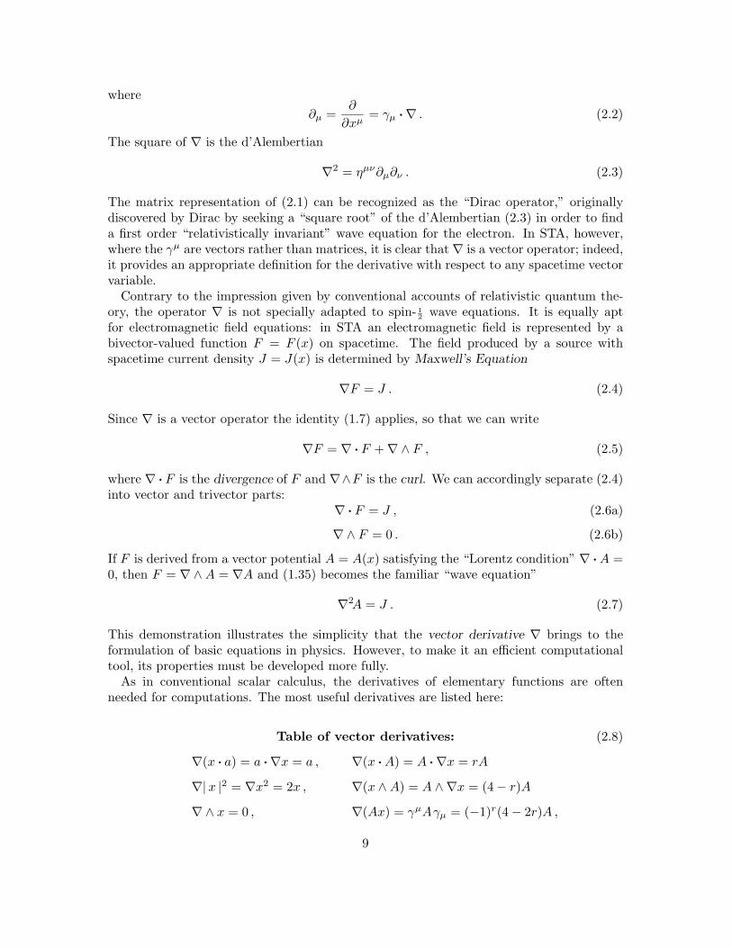
As in conventional scalar calculus, the derivatives of elementary functions are oftenneeded for computations. The most useful derivatives are listed here:

Table of vector derivatives: (2.8)

∇(x · a) = a ·∇x = a , ∇(x · A) = A ·∇x = rA

∇|x |2 = ∇x2 = 2x , ∇(x ∧ A) = A ∧∇x = (4 − r)A

∇∧ x = 0 , ∇(Ax) = γµAγµ = (−1)r(4 − 2r)A ,

9

∇x = ∇ · x = 4

∇|x |k = k|x |k−2x , ∇(

x

|x |k)

=4 − k

|x |k .

In the table, ∇ = ∂x, and obvious singularities at x = 0 are excluded; a is a “free vector”variable (i.e. independent of x), while A is a free r-vector.

The directional derivative a ·∇, that is, the “derivative in the direction of vector a” canbe obtained from ∇ by applying the inner product. Alternatively, the directional derivativecan be defined directly by

a ·∇F = a · ∂xF (x) =d

dτF (x + aτ)

∣∣∣τ=0

= limτ→0

F (x + aτ) − F (x)τ

, (2.9)

where F = F (x) is any multivector valued function. Then the general vector derivative canbe obtained from the directional derivative by using (2.8): thus,

∇F = ∂xF (x) = ∂aa · ∂xF (x) . (2.10)

This relation can serve as an alternative to the partial derivative in (2.1) for defining thevector derivative. Of course, the directional derivative has the same limit properties as thepartial derivative, including the rules for differentiating sums and products, but the explicitdisplay of the vector variable is advantageous in concept and calculation.

Equation (2.10) and the preceding equations above define the derivative ∂a with respectto any spacetime vector a. As already indicated, we reserve the symbol “x” for a vectorrepresenting a position in spacetime, and we use the special symbol ∇ ≡ ∂x for the derivativewith respect to this “spacetime point.” When differentiating with respect to any other vectorvariable a, we indicate the variable explicitly by writing ∂a. Mathematically, there is nodifference between ∇ and ∂a. However, there is often an important difference in physicalor geometrical interpretation associated with these operators.

The directional derivative (2.9) produces from F a tensor field called the differential ofF , denoted variously by

F(a) = Fa ≡ a ·∇F . (2.11)

As explained in the next section, the underbar notation serves to emphasize that F(a) is alinear function of a, though it is not a linear transformation unless it is vector valued. Theargument a may be a free variable or a vector field a = a(x).

The second differential Fb(a) = Fab is defined by

Fb(a) ≡ b ·∇F(a) − F(b ·∇a) = b · ∇F(a) , (2.12)

where the accents over ∇ and F serve to indicate that only F is differentiated and a is not.Of course, the accents can be dropped if a is a free variable. The second differential hasthe symmetry property

Fb(a) = Fa(b) . (2.13)

Using (1.14) and (1.17), this can be expressed as an operator identity:

(a ∧ b) · (∇∧∇) = [a ·∇, b ·∇] = 0 , (2.14)

10

where the bracket denotes the commutator. Differentation by ∂a and ∂b puts this identityin the form

∇∧∇ = 0 . (2.15)

These last three equations are equivalent formulations of the integrability condition forvector derivatives.

Since the derivative ∇ has the algebraic properties of a vector, a large assortment of“differential identities” can be derived by replacing some vector by ∇ in any algebraicidentity. The only caveat is to take proper account of the product rule for differentiation.For example, the product rule gives

∇ · (a ∧ b) = ∇ · (a ∧ b) + ∇ · (a ∧ b) ,

whence the algebraic identity (1.17) yields

a ·∇b − b ·∇a = ∇ · (a ∧ b) + a∇ · b − b∇ · a , (2.16)

The left side of this identity may be identified as a Lie bracket; a more general concept ofthe Lie bracket is introduced later on. Other identities will be derived as needed.

3. Linear Algebra

The computational and representational power of linear algebra is greatly enhanced by in-tegrating it with geometric algebra. In fact, geometric calculus makes it possible to performcoordinate-free computations in linear algebra without resorting to matrices. Integrationof the two algebras can be achieved with the few basic concepts, notations and theoremsreviewed below. However, linear algebra is a large subject, so we restrict our attention tothe essentials needed for gravitation theory.

Though the approach works for vector spaces of any dimension, we will be concernedonly with linear transformations of Minkowski space, which map spacetime vectors intovectors. We need a notation which clearly distinguishes linear operators and their productsfrom vectors and their products. To this end, we distinguish symbols representing a lineartransformation (or operator) by affixing them with an underbar (or overbar). Thus, for alinear operator f acting on a vector a, we write

fa = f(a) . (3.1)

As usual in linear algebra, the parenthesis around the argument of f can be included oromitted, either for emphasis or to remove ambiguity.

Every linear transformation f on Minkowski space has a unique extension to a linear func-tion on the whole STA, called the outermorphism of f because it preserves outer products.It is convenient to use the same notation f for the outermorphism and the operator that“induces” it, distinguishing them when necessary by their arguments. The outermorphismis defined by the property

f(A ∧ B) = (fA) ∧ (fB) (3.2)

for arbitrary multivectors A, B, andfα = α (3.3)

11

for any scalar α. It follows that, for any factoring A = a1 ∧ a2 ∧ . . . ∧ ar of an r-vector Ainto vectors,

f(A) = (fa1) ∧ (fa2) ∧ . . . ∧ (far) . (3.4)

This relation can be used to compute the outermorphism directly from the inducing linearoperator.

Since the outermorphism preserves the outer product, it is grade preserving, that is

f〈M 〉k = 〈 fM 〉k (3.5)

for any multivector M . This implies that f alters the pseudoscalar i only by a scalarmultiple. Indeed

f(i) = (det f)i or det f = −if(i) , (3.6)

which defines the determinant of f . Note that the outermorphism makes it possible todefine (and evaluate) the determinant without introducing a basis or matrices.

The “product” of two linear transformations, expressed by

h = gf , (3.7)

applies also to their outermorphisms. In other words, the outermorphism of a productequals the product of outermorphisms. It follows immediately from (3.6) that

det ( gf) = (det g)(det f) , (3.8)

from which many other properties of the determinant follow, such as

det (f−1) = (det f)−1 (3.9)

whenever f−1 exists.Every linear transformation f has an adjoint transformation f which can be extended

to an outermorphism denoted by the same symbol. The adjoint outermorphism can bedefined in terms of f by

〈Mf N 〉 = 〈N fM 〉 , (3.10)

where M and N are arbitrary multivectors and the bracket as usual indicates “scalar part.”For vectors a, b this can be written

b · f (a) = a · f(b) . (3.11)

Differentiating with respect to b we obtain, with the help of (2.8),

f (a) = ∂b a · f(b) . (3.12)

This is the most useful formula for obtaining f from f . Indeed, it might well be taken asthe preferred definition of f .

Unlike the outer product, the inner product is not generally preserved by outermorphisms.However, it obeys the fundamental transformation law

f [f(A) · B] = A · f (B) (3.13)

12

for (grade A) ≤ (grade B). Of course, this law also holds with an interchange of overbarand underbar. If f is invertible, it can be written in the form

f [A · B] = f−1(A) · f (B) . (3.14)

For B = i, since A · i = Ai, this immediately gives the general formula for the inverseoutermorphism:

f−1A = [f (Ai)](f i)−1 = (det f)−1f (Ai)i−1 . (3.15)

This relation shows explicitly the double duality involved in computing the inverse.Although all linear transformations preserve the outer product (by definition of the outer-

morphism (3.2)), only a restricted class preserves the inner product. This is called theLorentz group, and its members are called Lorentz transformations. The defining propertyfor a Lorentz transformation L is

(La) · (Lb) = a · (LLb) = a · b . (3.16)

This is equivalent to the operator condition

L = L−1 (3.17)

STA makes it possible to express any L in the simple canonical form

L(a) = εLaL−1 , (3.18)

where the multivector L is either even with ε = 1 or odd with ε = −1. This definesa double-valued homomorphism between Lorentz transformations L and multivectors±L, where the composition of two Lorentz transformations L1L2 corresponds to thegeometric product ±L1L2. Thus, the Lorentz group has a double-valued representationas a multiplicative group of multivectors. This multivector representation of the Lorentzgroup greatly facilitates the analysis and application of Lorentz transformations in STA.

From (3.18) it follows immediately that, for arbitrary multivectors A and B,

L(AB) = (LA)(LB) . (3.19)

Lorentz transformations therefore preserve the geometric product. This implies that (3.16)generalizes to

L(A · B) = (LA) · (LB) . (3.20)

in agreement with (3.14) when (3.17) is satisfied.From (3.18) it follows easily that

L(i) = εi , where ε = detL = ±1 . (3.21)

A Lorentz transformation L is said to be proper if ε = 1, and improper if ε = −1. It is saidto be orthochronous if, for any timelike vector v,

v · L(v) > 0 . (3.22)

13

A proper, orthochronous Lorentz transformation is called a Lorentz rotation (or a restrictedLorentz transformation). For a Lorentz rotation R the canonical form can be written

R(a) = RaR , (3.23)

where the even multivector R is called a rotor and is normalized by the condition

RR = 1 . (3.24)

The rotors form a multiplicative group called the Rotor group, which is a double-valuedrepresentation of the Lorentz rotation group (also called the restricted Lorentz group).

The most elementary kind of Lorentz transformation is a reflection n by a (non-null)vector n, according to

n(a) = −nan−1 . (3.25)

This is a reflection with respect to a hyperplane with normal n. A reflection

v(a) = −vav (3.26)

with respect to a timelike vector v = v−1 is called a time reflection. Let n1, n2, n3 bespacelike vectors which compose the trivector

n3n2n1 = iv . (3.27)

A space inversion vs can then be defined as the composite of reflections with respect tothese three vectors, so it can be written

vs(a) = n3n2n1an1n2n3 = ivavi = vav . (3.28)

Note the difference in sign between the right sides of (3.26) and (3.28). Although vs isdetermined by v alone on the right side of (3.28), the multivector representation of vs mustbe the trivector iv in order to agree with (3.18). The composite of the time reflection (3.26)with the space inversion (3.28) is the spacetime inversion

vst(a) = vsv(a) = −iai−1 = −a , (3.29)

which is represented by the pseudoscalar i. Note that spacetime inversion is proper but notorthochronous.

Two basic types of Lorentz rotation can be obtained from the product of two reflections,namely timelike rotations (or boosts) and spacelike rotations. For a boost

V (a) = V aV , (3.30)

the rotor V can be factored into a product

V = v2v1 (3.31)

of two unit timelike vectors v1 and v2. The boost is a rotation in the timelike plane contain-ing v1 and v2. The factorization (3.31) is not unique. Indeed, for a given V any timelike

14

vector in the plane can be chosen as v1, and v2 then computed from (3.31). Similarly, fora spacelike rotation

Q(a) = QaQ , (3.32)

the rotor Q can be factored into a product

Q = n2n1 (3.33)

of two unit spacelike vectors in the spacelike plane of the rotation.Note that the product, say n2v1, of a spacelike vector with a timelike vector is not a

rotor, because the corresponding Lorentz transformation is not orthochronous. Likewise,the pseudoscalar i is not a rotor, even though it can be expressed as the product of twopairs of vectors, for it does not satisfy the rotor condition (3.24).

Any Lorentz rotation R can be decomposed uniquely into the product

R = V Q (3.34)

of a boost V and spacelike rotation Q with respect to a given timelike vector v0 = v−10 . To

compute V and Q from R, first compute the vector

v = Rv0 = Rv0R . (3.35)

The timelike vectors v and v0 determine the timelike plane for the boost, which can thereforebe defined by

v = V v0 = V v0V = V 2v0 . (3.36)

This can be solved forV =

(vv0

) 12 = vw = wv0 , (3.37a)

where the unit vectorw =

v + v0

| v + v0 | =v + v0[

2(1 + v · v0)] 1

2(3.37b)

“bisects the angle” between v and v0. The rotor Q can then be computed from

Q = V R , (3.38)

so that the spacelike rotation satisfies

Qv0 = Qv0Q = v0 . (3.39)

This makes (3.36) consistent with (3.35) by virtue of (3.34).Equations (3.31) and (3.32) show how to parametrize boosts and spacelike rotations

by vectors in the plane of rotation. More specifically, (3.37a,b) parametrizes a boost interms of initial and final velocity vectors. This is especially useful, because the velocityvectors are often given, or are of direct relevance, in a physical problem. Another usefulparametrization is in terms of angle (Appendix B of [4]). Any rotor R can be expressed inthe exponential form

±R = e12 F =

∞∑k=0

1k!

(12F

)k, (3.40)

15

where F is a bivector parametrizing the rotation. The positive sign can always be selectedwhen F 2 = 0, and, according to (1.39), F can be written in the canonical form

F = (α + iβ)f where f2 = 1, (3.41)

α and β being scalar parameters. Since the timelike unit bivector f commutes with itsdual if , which is a spacelike bivector, the rotor R can be decomposed into a product ofcommuting timelike and spacelike rotors. Thus

R = V Q = QV , (3.42)

whereV = e

12 αf = cosh 1

2α + f sinh 12α , (3.43)

andQ = e

12 iβf = cos 1

2β + if sin 12β . (3.44)

The parameter α is commonly called the rapidity of the boost. The parameter β is theusual angular measure of a spatial rotation.

When F 2 = 0, equation (3.40) can be reduced to the form

R = e12 αf = 1 + 1

2αf , (3.45)

where f is a null bivector, and it can be expressed in the factored form (1.40). The twosigns are inequivalent cases. There is no choice of null F which can eliminate the minussign. The lightlike rotor in (3.45) represents a lightlike Lorentz rotation.

The spacelike rotations that preserve a timelike vector v0 are commonly called spatial ro-tations without mentioning the proviso (3.38). The set of such rotations is the 3-parameterspatial rotation group (of v0). More generally, for any given vector n, the subgroup ofLorentz transformations N satisfying

N(n) = NnN = n (3.46)

is called the little group of n. The little group of a lightlike vector can be parametrized asa lightlike rotor (3.40) composed with timelike and spacelike rotors.

The above classification of Lorentz transformations can be extended to more generallinear transformations. For any linear transformation f the composite ff is a symmetrictransformation. If the latter has a well defined square root S = (ff)

12 = S , then f admits

to the polar decompositionf = RS = S ′R , (3.47)

where R is a Lorentz rotation and S ′ = RSR−1. Symmetric transformations are, of course,defined by the condition

S = S . (3.48)

On Euclidean spaces every linear transformation has a polar decomposition, but on Min-kowski space there are symmetric transformations (with null eigenvectors) which do notpossess square roots and so do not admit a polar decomposition. A complete classificationof symmetric transformations is given in the next section.

16

4. Tensors and their classification

Our development of the “tensor concept” is somewhat unconventional, to allow us tointegrate it into the spacetime calculus and take full advantage of the algebra. We beginwith a definition which is more general than the usual one.

A tensor T of degree k is a multilinear, multivector-valued function T (a1, a2, . . . , ak) ofk vectors a1, a2, . . . , ak. This means that it is a linear function of each vector variableseparately. If it is skewsymmetric under interchange of any pair of variables, it can beregarded as a linear function L of a single k-vector variable; thus

L(a1 ∧ a2 ∧ . . . ∧ ak) = T (a1, a2 , . . . , ak) . (4.1)

This kind of function is called a k-form. Ordinarily k-forms are scalar-valued. The termmultiform can be used for the present generalization to multivector-valued functions. Ingeneral, then, a k-form

L(A) = L(〈A 〉k) (4.2)

is a multiform of degree k. This kind of function is fundamental to the theory of integrationset out in Section 6.

In ordinary tensor algebra, tensor addition is defined only for tensors with the same rankand degree. A tensor T of degree k has a definite rank r > k if it is (r − k)-vector valued,that is, if

T (a1, a2, . . . , ak) = 〈T (a1, a2, . . . , ak) 〉r−k . (4.3)

We call this a tensor of type r − k. All the tensors ordinarily considered in physics are ofthis type. Among the tensors to be encountered in later sections, the energy-momentumtensor T (a) and the gauge tensor h(a) are of type 2-1; the connection ω(a) is of type 3-1;and the curvature tensor R(a ∧ b) is of type 4-2. Of course, every multivector is triviallya tensor of degree zero. Every scalar-valued k-form is equivalent to a k-vector, as can beproved using relations laid out below.

Conventional tensor algebra employs the concept of rank alone, while the property ofdegree is attributed to forms alone; moreover, tensors and forms are treated as completelyseparate entities. Geometric algebra brings them under one roof. Two tensors (of degreer and s, say) can be multiplied using any of the various geometric products to form a newtensor of degree r+s. The conventional tensor product of “ranked tensors” is a tensor withrank equal to the sum of the ranks of the multiplicands, without any particular assignment ofdegree. Since the tensor product can always be expressed in terms of the geometric product[3], it need not be introduced as a separate concept. As conceived here a tensor is a purelyalgebraic object, without any of the transformation rules attached to its arguments as inconventional tensor analysis. From the algebraic viewpoint, the linear transformations andoutermorphisms of the preceding section are all tensors. Of course, the “product” of lineartransformations by functional composition is not a tensor product, although construction ofan outermorphism by outer products is. It should also be recognized that the terms “tensor”and “linear transformation” often indicate an important physical distinction when appliedto objects of identical algebraic structure. As a rule, physicists apply the term tensor toquantities representing some property of a physical system, while the term transformationis applied to changes in properties or their representation. For the purely algebraic purposes

17

of this section such a distinction is irrelevant. The coupling of tensors to transformationswill be considered later.

Tensors inherit algebraic properties automatically from their definition in terms of STA.The only problem outstanding is to give suitable names to these properties to facilitatedescription. The inner product a · T (a1, . . .) with a vector a reduces the grade of T butpreserves its rank. In fact, successive inner products with s = r − k vectors produces atensor of grade zero:

(a1, . . . , as) · T (as+1, . . . , ar) . (4.4)

We can regard (4.3) and (4.4) as different forms of one and the same tensor, for (4.3) canbe recovered from (4.4) by successive protractions. The protraction of T (with respect tothe first variable) is defined by

∂a ∧ T (a, . . . ) . (4.5)

Unless the result vanishes, protraction raises the grade but preserves the rank. Contraction,defined by

∂a · T (a, . . . ) , (4.6)

lowers the rank by 2 and the grade by 1. Of course, this operation is not defined if thegrade of T is zero.

It will be recognized that the protraction (4.5) is just a curl while the contraction (4.6) isjust a divergence. This introduction of new names is justified, nevertheless, by their uniqueapplication to multilinear functions. In particular, note that these operations completelyremove a tensor’s functional dependence on one variable. Another type of contraction,which eliminates two explicit variables, is defined by

∂a · ∂bT (. . . a, . . . , b . . . ) = T (. . . ∂a, . . . , a . . . ) = T (. . . γµ, . . . , γµ . . . ) . (4.7)

This is equivalent to the standard definition of contraction in tensor analysis. Note that thecontraction using the derivative is equivalent to the sum over a frame and its reciprocal,as defined by (1.27). In later sections this type of contraction will arise mainly fromcombinations of protractions and contractions of the “divergence type” (4.6), to which it isequivalent in some cases.

We now have enough mathematical apparatus for systematic classification of all tensors.However, we restrict our attention to those tensors of importance in gravitation theory — inparticular, the energy-momentum tensor and the curvature tensor. Algebraic classificationsof these tensors have been thoroughly worked out in the literature [16]. However, it willbe seen that STA brings a new perspective to the subject. The algebraic classification ofcurvature tensors will be discussed in Section 11. The rest of this section is devoted tothe classification of type 2-1 tensors; this includes all linear transformations as well as theenergy-momentum tensor.

For a type 2–1 tensor f , protraction produces an “invariant” bivector

F = ∂a ∧ f(a) , (4.8)

while the contraction produces the trace

f0 ≡ Tr f = ∂a · f(a) . (4.9)

18

The inner product of (4.8) with a vector recovers the skewsymmetric part of f :

f−(a) = 12

[f(a) − f (a)

]= 1

2a · F . (4.10)

From the symmetric partf+(a) = 1

2

[f(a) + f (a)

], (4.11)

we can extract a traceless part

f⊕ = f+ − 1n

f0 1 , (4.12)

where 1 is the identity operator and n = Tr 1. Putting all the parts together, we have thewell known invariant decomposition

f = f⊕ +1n

f0 1 + f− . (4.13)

This kind of decomposition is especially useful when the bivector F in (4.8) and (4.10) hasa direct physical interpretation. An important example, to be considered in Part III, is thedeformation rate tensor, for which the protraction can be identified with vorticity.

As an alternative to the decomposition (4.13), the polar decomposition (3.47) is signifi-cant in other physical problems. In both cases a symmetric tensor appears — additively inone case, and multiplicatively in the other. A complete classification of symmetric tensorsinvolves much more than simply separating off a traceless part as in (4.12). There are threemajor types, as is now described.

Type I

A symmetric tensor S is said to be of type I if it admits to the “spectral decomposition”

S =∑

k

λk ek , (4.14)

where the λk = 〈λk 〉0 are real scalars and the ek are irreducible projection operators withthe properties

Idempotence: e2k = ek, (4.15a)

Orthogonality: ej ek = 0 for j = k, (4.15b)

Completeness:∑

k ek = 1, (4.15c)

Eigenvectors: ej(ek) = δjkek. (4.15d)

Therefore S has a unique set of eigenvectors ek satisfying

Sek = λkek . (4.16)

The eigenvectors compose an orthogonal basis e0, e1, e2, e3 for Minkowski space.

19

Type I tensors S and S ′, related by a Lorentz rotation R according to

S ′ = RSR−1 =∑

k

λk e ′k , (4.17)

are equivalent in the sense that they have the same spectrum of eigenvalues λk. Subtypesare distinguished by special properties of the eigenvalues, such as positivity or degeneracy.This gives a complete classification of type I tensors.

Geometric algebra makes it possible to derive the projection operators from the eigen-vectors; thus,

ek(a) = e−1k ek · a = eke−1

k · a = 12 (a + ekae−1

k ) . (4.18)

Also, outermorphisms facilitate the analysis and applications of symmetric transformations.For example, the bivectors

eij ≡ ei ∧ ej = eiej (4.19)

can be regarded as eigenbivectors of S satisfying (for i = j)

S(eij) = λiλjeij . (4.20)

Similarly, there are eigentrivectors

S(eijk) = λiλjλkeijk . (4.21)

Finally, for the pseudoscalar i we have

S(i) = λ0λ1λ2λ3i , so det S = λ0λ1λ2λ3 . (4.22)

For degenerate eigenvalues λi = λj , the spectral form (4.14) can be simplified by introducingthe bivector projection

e ij(a) ≡ e−1ij (eij · a) = e i(a) + ej(a), (4.23)

so that two terms in the sum are reduced to one according to

λi e i + λj ej = λi e ij , (4.24)

and the arbitrariness in choosing eigenvectors in the eij-plane is eliminated. Note theoutermorphism properties

ek(a ∧ b) = 0 , (4.25)

e ij(a ∧ b) = eij−1eij · (a ∧ b) , (4.26)

e ij(a ∧ b ∧ c) = 0 . (4.27)

For vector spaces with a Euclidean inner product, all symmetric tensors are of type I.However, for spacetime the existence of null vectors leads to other types.

Before continuing the classification, it is convenient to make a short excursion into theproperties of null vectors. Two null vectors k, k∗ are said to be a conjugate pair if

k2 = k∗2 = 0 , k · k∗ = 1 . (4.28)

20

These vectors determine a unique timelike bivector

K ≡ k ∧ k∗ , (4.29)

withK2 = (k · k∗)2 = 1 . (4.30)

Also,Kk = K · k = k and Kk∗ = −k∗ . (4.31)

Therefore k and k∗ are eigenvectors of the tensor

K−(a) ≡ K · a (4.32)

with real eigenvalues ±1, even though K− is a skew symmetric tensor. Relations (4.28)and (4.29) can be combined into

kk∗ = 1 + K , (4.33)

which has the idempotence property

(kk∗)2 = (1 + K)2 = 2kk∗ . (4.34)

All the above relations between k and k∗ are invariant under the rescaling

k → αk , k∗ → 1α

k∗ , (4.35)

by an arbitrary nonzero scalar α.By analogy with the structure of the projection operators ek in (4.18), we can construct

from k and k∗ the elementary tensors

k(a) ≡ kk · a = 12kak and k∗(a) ≡ k∗k∗ · a . (4.36)

These tensors are not projections because, instead of being idempotent, they are nilpotent,satisfying

k2 = 0 = k∗2 . (4.37)

However, they are also symmetric tensors and are obviously not of type I.Two other elementary tensors can be formed from k and k∗, namely

k∗(a) ≡ kk∗ · a (4.38a)

and its adjointk ∗(a) ≡ k∗k · a . (4.38b)

These tensors are idempotent, but they are not symmetric. However, they do have thesymmetric combination

K(a) ≡ KK · a = k∗(a) + k ∗(a) , (4.39)

which is just the projection onto the K-plane.

21

We are now ready to continue the classification of symmetric tensors. To simplify com-parison with type I we identify the K-plane with the e30-plane in the notation of (4.19).

Type II

A symmetric tensor of type II has the canonical form

S = S0 + λ1 e1 + λ2 e2 , (4.40)

where the ek satisfy (4.15a–d) and

S0 ek = ekS0 = 0 . (4.41)

It has an irreducible eigenbivector K satisfying

S(K) = λ20K . (4.42)

In other words, S leaves a timelike plane invariant. The eigenbivector K is irreducible inthe sense that, unlike the eigenbivectors eij of a type I tensor, it cannot be factored intoa product of two eigenvectors. The dual of K is proportional to e12, so it is a reducibleeigenbivector satisfying

S(iK) = λ1λ2iK . (4.43)

The type II tensors fall into three distinct subtypes, which can be characterized by specifyingthe operator S0 in terms of the three distinct elementary symmetric operators defined by(4.36) and (4.39).

Type II±

S0 = K[λ0 ± k] = λ0K ± k . (4.44)

In this case there is exactly one null eigenvector when λ0 = 0,

Sk = S0k = λ0k . (4.45)

If both k and k∗ were eigenvectors we would have a type I tensor. The coefficient of thelast term in (4.44) has been set to unit magnitude without loss of generality, because k canbe rescaled using (4.35) without affecting K in the other term. Because rescaling cannotchange the sign of the coefficient, there are two distinct cases II±.

Type II0

S0 = λ0K + β(k∗ − k) . (4.46)

In this case, with β nonzero, there are no eigenvectors in the K-plane. Rescaling has beenused to set the coefficients of k and k∗ to the same magnitude, but they are necessarilyopposite in sign. The characteristic equation for S0 has complex roots z = λ0 ± iβ, though

22

the unit imaginary here is devoid of geometric meaning and cannot be identified with theunit pseudoscalar. Instead this “imaginary” originates from the combination of nilpotentoperators on the right side of (4.46).

Type III

In this case there is a single irreducible eigentrivector K1, which can be written in theform

K1 = k ∧ k∗ ∧ e1 = Ke1 = −ie2 . (4.47)

Defining

K1(a) ≡ K1K−11 · a , (4.48)

k1(a) ≡ ke−11 · a and k 1(a) ≡ e−1k · a , (4.49)

a type III tensor can be put in the canonical form

S = λ1K1 + k1 + k 1 + λ2 e2 . (4.50)

Here the symmetric tensor k1 + k 1 has been scaled to unity without loss of generality. Itis readily verified that

S(K1) = λ31K1 , (4.51)

and the 3-dimensional hyperplane “spanned” by K1 “contains” exactly one eigenvector

S(k) = λ1k (4.52)

and one eigenbivectorS(k ∧ e1) = λ2

1k ∧ e1 . (4.53)

In addition, there is one other eigenvector

S(e2) = λ2e2 (4.54)

and one other eigenbivectorS(k ∧ e2) = λ1λ2k ∧ e2 . (4.55)

Equations (4.53) and (4.55) characterize two invariant null planes intersecting in the nullline of k.

This completes the classification of the main types of symmetric tensors on Minkowskispace. An important application is to the classification of energy-momentum tensors. Forany nonspacelike vector u, a given energy-momentum tensor T (u) is usually assumed (atleast tacitly) to satisfy the conditions

u · T (u) ≥ 0 , (4.56)

[T (u) ]2 ≥ 0 . (4.57)

The first condition ensures that the energy density is never negative. This is formallyequivalent to the condition (3.22) for a Lorentz transformation to be orthochronous, though

23

equality never occurs in that case. Accordingly, we refer to any tensor T (a) as orthochronousif it satisfies (4.56). The conditions (4.56) eliminate classes II−, II0 and III. Moreover, forclasses I and II+ they require that

λ0 ≥ |λk | (4.58)

for k = 1, 2, 3 in the first case, or k = 1, 2 in the second.As an important example, consider the energy-momentum tensor for an arbitrary elec-

tromagnetic field F , which can be put in the form

T (a) = −12FaF = − 1

2faf , (4.59)

where the last equality arises on using the canonical form (1.39). There are two cases.When f = e3e0 is a timelike bivector, (4.49) has two pairs of doubly degenerate eigenvalues

λ0 = λ3 = 12f2 = −λ1 = −λ2 , (4.60)

so that it is a type I tensor. When f is a null bivector with the form (1.40), (4.59) can bewritten

T (a) = 12ekake = ekk · ae = kk · a , (4.61)

so that it is a type II+ tensor of the most elementary kind (4.36).

5. Transformations on spacetime

This section describes the apparatus of geometric calculus for handling transformationsof spacetime and the induced transformations of multivector fields on spacetime. We con-centrate on the mappings of 4-dimensional regions, including the whole of spacetime, butthe apparatus applies with only minor adjustments to the mapping of any submanifoldin spacetime. Throughout, we assume whatever differentiability is required to performindicated operations, so that we might as well assume that the transformations are diffeo-morphisms and defer the analysis of discontinuities in derivatives. We therefore assumethat all transformations are invertible unless otherwise indicated.

Let f be a diffeomorphism which transforms each point x in some region of spacetimeinto another point x′, as expressed by

f : x → x′ = f(x) . (5.1)

This induces a linear transformation of tangent vectors at x to tangent vectors at x′, givenby the differential

f : a → a′ = f(a) = a ·∇f . (5.2)

More explicitly, it determines the transformation of a vector field a = a(x) into a vectorfield

a′ = a′(x′) ≡ f [a(x); x] = f [a(f−1(x′)); f−1(x′) ] . (5.3)

The outermorphism of f determines an induced transformation of specified multivectorfields. In particular,

f(i) = Jf i, where Jf = det f = −ifi (5.4)

24

is the Jacobian of f .The transformation f also induces an adjoint transformation f which takes tangent

vectors at x′ back to tangent vectors at x, as defined by

f : b′ → b = f (b′) ≡ ∇f · b′ = ∂xf(x) · b′ . (5.5)

More explicitly, for vector fields

f : b′(x′) → b(x) = f [ b′(x′); x ] = f [ b′(f(x)); x ] . (5.6)

The differential is related to the adjoint by

b′ · f(a) = a · f (b′) . (5.7)

According to (3.15), f determines the inverse transformation

f−1(a′) = f (a′i)(Jf i)−1 = a . (5.8)

Also, however,f−1(a′) = a′ · ∂x′f−1(x′) . (5.9)

Thus, the inverse of the differential equals the differential of the inverse.Since the adjoint maps “backward” instead of “forward,” it is often convenient to deal

with its inversef−1 : a(x) → a′(x′) = f−1 [ a(f−1(x′)) ] . (5.10)

This has the advantage of being directly comparable to f . Note that it is not necessary todistinguish between f−1 and f −1.

Thus, we have two kinds of induced transformations for multivector fields: The first, by f ,is commonly said to be contravariant, while the second, by f or f −1, is said to be covariant.The first is said to “transform like a vector,” while the second is said to “transform likea covector.” The term “vector” is thus associated with the differential while “covector” isassociated with the adjoint. This linking of the vector concept to a transformation law isaxiomatic in ordinary tensor calculus. In geometric calculus, however, the two concepts arekept separate. The algebraic concept of vector is determined by the axioms of geometricalgebra without reference to any coordinates or transformations. Association of a vector ora vector field with a particular transformation law is a separate issue.

The transformation of a multivector field can also be defined by the rule of directsubstitution: A field F = F (x) is transformed to

F ′(x′) ≡ F ′(f(x)) = F (x) . (5.11)

Thus, the values of the field are unchanged — although they are associated with differentpoints by changing the functional form of the field. For the purposes of “gauge gravitytheory” discussed in the next section, it is very important to note that the alternativedefinition F ′(x) ≡ F (x′) is adopted in [1]. Each of these two alternatives has something torecommend it.

25

Directional derivatives of the two different functions in (5.11) are related by the chainrule:

a ·∇F = a · ∂xF ′(f(x)) = (a ·∇xf(x)) ·∇x′F ′(x′) = f(a) ·∇′F ′ = a′ ·∇′F ′ . (5.12)

The chain rule is more simply expressed as an operator identity

a ·∇ = a · f (∇′) = f(a) ·∇′ = a′ ·∇′ . (5.13)

Differentiation with respect to the vector a yields the general transformation law for thevector derivative:

∇ = f (∇′) or ∇′ = f −1(∇) . (5.14)

This is the most basic formulation of the chain rule, from which its many implications aremost easily derived. All properties of induced transformations are essentially implicationsof this rule, including the transformation law for the differential, as (5.13) shows.

The rule for the induced transformation of the curl is derived by using the integrabilitycondition (2.15) to prove that the adjoint function has vanishing curl; thus, for the adjointof a vector field,

∇ ∧ f (a′) = ∇b ∧ fb(a′) = ∇b ∧∇cfcb · a′ = ∇∧∇f · a′ = 0 . (5.15)

The transformation rule for the curl of a vector field a = f (a′) is therefore

∇∧ a = ∇∧ f (a′) = f (∇′ ∧ a′) . (5.16)

To extend this to multivector fields, note that the differential of an outermorphism is notitself an outermorphism; rather it satisfies the “product rule”

fb(A′ ∧ B′) = fb(A′) ∧ f (B′) + f (A′) ∧ fb(B′) . (5.17)

Therefore, it follows from (5.15) that the curl of the adjoint outermorphism vanishes, and(5.16) generalizes to

∇∧ A = f (∇′ ∧ A′) or ∇′ ∧ A′ = f −1(∇∧ A) , (5.18)

where A = f (A′). Thus, the outermorphism of the curl is the curl of an outermorphism.The transformation rule for the divergence is more complex, but it can be derived from

that of the curl by exploiting the duality of inner and outer products (1.12) and the trans-formation law (3.14) relating them. Thus,

f (∇′ ∧ (A′i)) = f [ (∇′ · A′)i ] = f −1(∇′ · A′)f (i) .

Then, using (5.18) and (5.4) we obtain

∇∧ f (A′i) = ∇∧ [ f−1(A′)f (i) ] = ∇ · (JfA)i .

For the divergence, therefore, we have the transformation rule

∇′ · A′ = ∇′ · f(A) = Jf−1 f [∇ · (JfA) ] = f [∇ · A + (∇ lnJf ) · A ] , (5.19)

26

where A′ = f(A). This formula can be separated into two parts:

∇′ · f (A) = f [ (∇ ln Jf ) · A ] = (∇′ ln Jf ) · f(A) , (5.20)

∇′ · f(A) = f(∇ · A) . (5.21)

The whole may be recovered from the parts by using the following generalization of (5.13)(which can also be derived from (3.14)):

f(A) ·∇′ = f(A ·∇) . (5.22)

6. Directed Integrals and the Fundamental Theorem

In the theory of integration, geometric calculus absorbs, clarifies and generalizes thecalculus of differential forms. Only the essentials are sketched here; details are given in [3],and [7] discusses the basic concepts at greater length with applications to physics.

The integrand of any integral over a k-dimensional manifold is a differential k-form

L = L(dkx) = L [ dkx; x ], (6.1)

where dkx is a k-vector-valued measure on the manifold. If the surface is not null at x, wecan write

dkx = Ik | dkx | , (6.2)

where Ik = Ik(x) is a unit k-vector field tangent to the manifold at x, and | dkx | is anordinary scalar-valued measure. Thus, dkx describes the direction of the tangent spaceto the manifold at each point. For this reason it is called a directed measure. Since theintegrals are defined from weighted sums, the integrand L(dkx) must be a linear functionof its k-vector argument; accordingly it is a k-form as defined in Section 4. Of course, thevalues of L may vary with x, as indicated by the explicit x-dependence shown on the rightside of (2.17).

The exterior differential of a k-form L is a (k + 1)-form dL defined by

dL = L[ (dk+1x) · ∇ ] = L[ (dk+1x) · ∇; x ] , (6.3)

where the accent indicates that only the implicit dependence of L on x is differentiated.The exterior derivative of any “k-form” which is already the exterior derivative of anotherform necessarily vanishes, as is expressed by

d2L = 0. (6.4)

This is an easy consequence of the integrability condition (2.15); thus,

d2L = dL[ (dk+1x) · ∇ ] = L[ (dk+1x) · (∇ ∧ ∇) ] = 0 .

27

The Fundamental Theorem of Integral Calculus (also known as the “Boundary Theorem”or the “Generalized Stokes’ Theorem”) can now be written in the compact form

∫dL =

∫dL (dk+1x) =

∮L(dkx) =

∮L . (6.5)

This says that the integral of any k-form L over a closed k-dimensional manifold is equalto the integral of its exterior derivative over the enclosed (k + 1)-dimensional manifold. Itfollows from (6.4) that this integral vanishes if L = dN where N is a (k − 1)-form.

To emphasize their dependence on a directed measure, the integrals in (6.5) may becalled directed integrals. In conventional approaches to differential forms this dependenceis disguised and all forms are scalar-valued. For that special case we can write

L = 〈A dkx 〉 = (dkx) · A(x) , (6.6a)

where A = A(x) is a k-vector field. Then

dL = [(dk+1x) ·∇ ] · A = (dk+1x) · (∇∧ A) . (6.6b)

In this case, therefore, the exterior derivative is equivalent to the curl.An alternative form of the Fundamental Theorem called “Gauss’s Theorem” is commonly

used in physics. If L is a 3-form, its 3-vector argument can be written as the dual of avector, and a tensor field T (n) = T [n(x); x] can be defined by

T (n) = L(in) . (6.7)

According to (6.2) we can write

d4x = i | d4x | and d3x = in−1 | d3x | , (6.8)

where n is the outward unit normal defined by the relation I3n = I4 = i. Substitution into(6.5) then gives Gauss’s Theorem:

∫T (∇) | d4x | =

∮T (n−1) | d3x | . (6.9)

where n−1 = εn with signature ε. Though T (∇) may be called the “divergence of the tensorT ,” it is not generally equivalent to the divergence as defined earlier for multivector fields.However, if L is scalar-valued as in (6.6a), then (6.7) implies that

T (n) = n · a , (6.10a)

where a = a(x) = A(x)i is a vector field. In this case, we do have the divergence

T (∇) = ∇ · a . (6.10b)

Note that duality has changed the curl in (6.6b) into the divergence in (6.10b).

28

A change of integration variables in a directed integral is a transformation on a differentialform by direct substitution. Thus, for the k-form defined in (6.1) we have

L′(dkx′) = L(dkx) , (6.11)

wheredkx′ = f(dkx) or dkx = f−1(dkx′) (6.12)

In other words, L′ = Lf−1 or, more explicitly,

L′(dkx′; x′) = L[ f−1(dkx); f−1(x) ] = L(dkx;x) . (6.13)

The value of the integral of (6.11) is thus unaffected by the change of variables,

∫L′(dkx′) =

∫L[ f−1(dkx′) ] =

∫L(dkx) . (6.14)

The exterior derivative and hence the fundamental theorem are likewise unaffected. Inother words,

dL′ = dL . (6.15)

This follows from(dkx′) ·∇′ = f(dkx) · f (∇) = f [ (dkx) ·∇ ] (6.16)

anddf(dkx) = f [ (dkx) · ∇ ] = 0 . (6.17)

Like (6.4), the last equation is a consequence of the integrability condition.

Part II. INDUCED GEOMETRY ON FLAT SPACETIME

7. Gauge Tensor and Gauge Invariance

We shall regard (Minkowski) spacetime as a mathematical device for representing theordering of physical events. A spacetime map represents the ordering of particular eventsby points (vectors) in spacetime. No other physical property is attributed to spacetimeitself. Instead, all other properties of physical entities are represented as fields on spacetimeor as constructs from such fields.

A given ordering of events can be represented by a map in many different ways, just asthe surface of the earth can be represented by Mercator projection, stereographic projectionor many other equivalent maps. As the physical world is independent of the way weconstruct our maps, we seek a physical theory which is equally independent. This idea canbe formulated as a general theoretical principle, which, with deference to Einstein, we dub

29

The Principle of General Invariance (PGI): The equations ofphysics must be invariant under arbitrary smooth remappings of eventsonto spacetime.

The precise mathematical implementation of this principle leads naturally to a geometrictheory of gravitation, as we shall show.

A smooth remapping of spacetime is a diffeomorphism of spacetime onto itself. Themathematical apparatus for handling such transformations was set out in Section 5. Wesaw there that, via the chain rule, differentiation automatically induces transformations ofvectors and covectors. For example, let x = x(τ) be a timelike curve representing a particlehistory. According to (5.2), the diffeomorphism (5.1) induces the transformation

x. =

dx

dτ→ x

.′ = f(x.) . (7.1)

Thus the description of particle velocity by x. is “covariant” under spacetime diffeomor-

phisms. An “invariant” description by a velocity vector v = v(x(τ)) can be achieved byintroducing an invertible tensor field h such that

x. = h(v), (7.2)

while supposing that h undergoes the induced transformation

f : h → h′ = f h , (7.3)

where it is understood that h is a function of x while, using (5.1), h′ is expressed as afunction of x′. Then (7.1) implies that

x.′ = h′(v) (7.4)

where v = v(f−1(x′)) ≡ v(x′) has the same value as in (7.2), but it is taken as a function

of x′(τ) instead of x(τ). To distinguish the velocity representation x. from

v = h−1(x.) , (7.5)

let us refer to x. as the map velocity. Otherwise the term velocity designates v. The

normalizationv2 = 1 (7.6)

fixes the scale on the parameter τ , which can therefore be interpreted as proper time.The transformation of h defined by (7.3) is called a “position gauge transformation,” and

h (or h) is called the “gauge tensor” or simply the “gauge” on spacetime. Actually, theterm “gauge” is more appropriate here than elsewhere in physics, because h does indeeddetermine the “gauging” of a metric on spacetime. To see that, use (7.1) in (7.5) to derivethe following expression for the invariant line element on a timelike particle history:

dτ2 = [ h−1(dx) ]2 = dx · g(dx) , (7.7a)

whereg = h−1h−1 (7.7b)

30

is a symmetric metric tensor. Our formulation indicates the gauge as a more fundamentalgeometric entity than the metric, and this view will be confirmed by developments below.Einstein has taught us to interpret the metric tensor physically as a gravitational potential,making it easy and natural to transfer this interpretation to the gauge tensor. Some readerswill recognize h as equivalent to a “vierbein field,” which has been proposed before torepresent gravitational fields on flat spacetime [17]. However, availability of the spacetimecalculus makes all the difference in turning this idea into a practical reality.

To verify that (7.7a) is equivalent to the standard invariant line element in general rela-tivity, coordinates can be introduced. Let x = x(x0, x1, x2, x3) be a parametrization of thepoints, in some spacetime region, by an arbitrary set of coordinates xµ. Partial deriva-tives then give tangent vectors to the coordinate curves ∂µx, which, in direct analogy to(7.2) and (7.5), determine a set of position gauge invariant vector fields gµ according tothe equation

∂µx =∂x

∂xµ= h(gµ) , (7.8)

or, equivalently, bygµ = h−1(∂µx) . (7.9)

The components for this coordinate system are then given by

gµν = gµ · gν = (∂µx) · g(∂νx) . (7.10)

Therefore, with dx = dxµ∂µx, the line element (7.7a) can be put in the familiar form

dτ2 = gµνdxµdxν . (7.11)

More about coordinates in Part III.The adjoint of (7.3) gives us the transformation rule

h′ = hf . (7.12)

Applying this to the vector derivative ∇ with its transformation rule (5.14), we can definea position gauge invariant derivative by

/ ≡ h(∇) = h′(∇′) . (7.13)

Applied to a gauge invariant field ϕ = ϕ(x) this gives the position gauge invariant gradient

/ϕ ≡ h(∇ϕ) = h′(∇′ϕ′) . (7.14)

where ϕ′ = ϕ(x′) = ϕ(f−1(x′)). From the operator / we obtain a position gauge invariantdirectional derivative

a · / = a · h(∇) = (ha) ·∇ , (7.15)

where a is a “free vector,” which is to say that it can be regarded as constant or astransforming by substitution:

a′ = a′(x′) = a(f−1(x′)) = a(x) = a . (7.16)

31

The transformation rules (7.3) and (7.12) now give us

h′(a′) ·∇′ = [f h(a)] ·∇′ = h(a) · f (∇′) = h(a) ·∇,

which makes the invariance of (7.15) explicit.For any field F = F (x(τ)) defined on a particle history x(τ), the chain rule gives the

operator relationd

dτ= x

. ·∇ = h(v) ·∇ = v · / , (7.17)

so thatdF

dτ= v · /F . (7.18)

For F (x) = x, this givesdx

dτ= v · /x = (hv) ·∇x = hv , (7.19)

recovering (7.2).Besides the gauge transformation (7.3) or (7.12), there is another kind of gauge trans-

formation that leaves invariant the form of the above equations. From the discussion inSection 3, we know that the velocity normalization (7.6) is invariant under the Lorentzrotation

R : v = v(x) → v′ = R v = R (v(x); x) . (7.20)

Here, however, v is a vector field and the rotation R varies smoothly from point to pointbut is otherwise arbitrary. Let us signify this local variability of R by calling it a localLorentz rotation. Since R = R−1, the relation

x. = h(v) = h′(v′)

is left invariant by (7.20) if it is accompanied by the adjoint gauge change

h′ = hR . (7.21)

This kind of gauge transformation leaves the metric tensor (7.7b) invariant, since

(R h)−1(hR)−1 = h−1RR h−1 = h−1h−1 = g .

The gauge change (7.21) does not entail any remapping of spacetime points. Rather, via(7.20), it induces a change of direction at each spacetime point. We express this fact byreferring to (7.21) as a directional gauge change. This name distinguishes it from thepositional gauge change (7.3). Of course, the two kinds are combined in the most generalspacetime gauge change:

h′ = f hR . (7.22)

The idea expressed by (7.2), that the tangent vector x. to a particle history is not generally

collinear with its velocity v, is unfamiliar to most physicists. It may be of some comfort,therefore, to note that if x

. is timelike, as is usual for a material particle except in an extremegravitational field, then it can be aligned with v by a local Lorentz rotation along a segment

32

of the particle history. In that case the gauge is set so that v is an eigenvector of the gaugetensor, and (7.3) reduces to

x. = h(v) = γv . (7.23)

The eigenvalue γ evidently characterizes a gravitationally induced shift in the particle’sproper time rate, as does the equation (7.7a) for the invariant line element.

In general, the noncollinearity of v and x. in (7.2) signifies the presence of a gravitational

field, so it cannot be transformed away globally. A major problem for gravitation theory istherefore to ascertain precisely the global constraints on gauge freedom induced by variousphysical assumptions. Just as positional gauge freedom has been theoretically formalizedby the Principle of General Invariance (PGI), directional gauge freedom can be formalizedby

The Principle of Local Relativity (PLR): The equations of physicsmust be covariant (i.e. form invariant) under local Lorentz rotations.

This principle, first formulated with spacetime calculus in [4], can be interpreted physicallyas asserting that the relative directions of multivector fields representing physical propertiesat each spacetime point have an absolute physical significance, while the comparison ofdirections at different points generally does not. Equation (3.19) tells us that the geometricproduct is preserved by Lorentz rotations at a point, so that relative directions at eachspacetime point are invariant. Obviously, the position dependence of local Lorentz rotationsimplies that this is not so for relative directions at different points — although solutions tothe equations of physics may determine some physical significance for this so-called “distantparallelism,” as in the case of flat spacetime.

An important consequence of local relativity is that, although the operator / defined by(7.13) is positionally gauge invariant, it is not directionally invariant. The gauge change(7.21) induces a transformation of / to

/′= R / . (7.24)

Except when operating on scalars, as in (7.14), / is not directionally covariant. To satisfythe Principle of Local Relativity a directionally covariant differential operator must bedefined. That will be the main task in the next section.

Our two general gauge principles PGI and PLR are obviously closely related to Einstein’sprinciples of general and special relativity. To make the relation definite, let us regard thePGI as a gauge formulation of Einstein’s Principle of General Covariance (PGC). Recallthat Einstein regarded the PGC as a cornerstone of his general theory, but that shortlyafter publication Kretschmann and Cartan argued that it is devoid of physical content.Einstein retreated but continued to assert that the PGC plays an essential heuristic role inhis theory. Precisely what that role might be has remained obscure to this day. Mutuallyincompatible attempts to pin it down by various commentators range as far as outrightrejection of Einstein’s claim. All obscurity is removed, however by the restatement of thePGC as the PGI, with its precise formulation in terms of the spacetime calculus. We haveseen that implementation of the PGI requires the existence of a gauge tensor and of thegeometry it entails. This is a nontrivial heuristic consequence of great importance, for it isthe main idea driving the construction of the whole gauge theory of gravitation in [1]. Thus

33

it provides strong grounds for asserting that: Once again, Einstein’s physical intuition isunerring — outstripping the analysis of his critics.

Another obscure point in Einstein’s work which has been endlessly discussed, is therelation between his Special and General Theories. Gauge theory throws new light on thisissue with its sharp distinctions between positional and directional gauge transformations.Since the latter are Lorentz rotations R, the PLR can be regarded as a generalizationof the Principle of Special Relativity, to which it reduces when each R is a constant. Thejustification for this reduction is that, in the absence of gravity, there is a preferred gaugeh = 1 and all points are geometrically equivalent. From (7.21), therefore, all other gaugesare given by h′ = R. This fact can be interpreted as an expression of the isotropy of thespacetime gauge. Homogeneity of the spacetime gauge is expressed by the existence ofpreferred position gauge changes, called Poincare transformations, with the general form

x′ = f(x) = Rx + c , (7.25)

where R and c are constant. The differential of this transformation is

f = R . (7.26)

Thus, positional and directional gauge changes merge in Special Relativity. Conversely,the Lorentz transformations of Special Relativity are generalized in two distinctly differentways by General Relativity. This fact is obscured in the usual covariant formulation interms of tensor analysis.

8. Covariant Derivative and Parallel Transport

To satisfy the Principle of Local Relativity we construct a new differential operator whichis covariant (i.e. form invariant) under directional gauge transformations. Generalizing(7.20) and using (3.22), the directional gauge change of an arbitrary Multivector fieldA = A(x) can be written

R (A) = RAR (8.1)

where R = R(x) is a rotor field. The directional derivative of the rotor can be written inthe form

a · /R = 12RΩ(a) , (8.2)

where the quantity

Ω(a) = 2R a · /R = −2(a · /R)R = −Ω(a) (8.3)

is a bivector field. Therefore, the directional derivative of R (A) can be written

a · /R (A) = R [Ω(a) × A ] = [R Ω(a) ] × R (A) (8.4)

where × is the commutator product defined by (1.32). According to (1.36), the commutatorproduct with Ω(a) is grade-preserving.

34

A gauge covariant directional derivative can now be defined in a standard way by intro-ducing a so-called gauge field ω(a) = ω(a;x) with the operator definition

a · D ≡ a · / + ω(a) × . (8.5)

Applied to any multivector field A this gives, of course,

a · DA = a · /A + ω(a) × A . (8.6)

The idea is to assign to ω(a) the gauge transformation rule

ω′(a′) = R (ω(a) − Ω(a)) = Rω(a)R − 2(a · /R)R (8.7)

with a′ = Ra, so that its last term cancels (8.4) and a · D satisfies the gauge covariancecondition

a′ · D′R (A) = R (a · DA) (8.8)

witha′ · D′ = a′ · /′

+ ω′(a′)× = a · / + ω′(Ra) × . (8.9)

Clearly the gauge field ω(a) must be bivector-valued to satisfy (8.7).To distinguish a · D from the directional derivative defined by (7.15) we call it the direc-

tional coderivative. A vectorial coderivative D can then be defined by

D = ∂aa · D = / + ∂aω(a)× , (8.10)

where / is given by (7.13). In geometry the gauge field ω(a) is called a linear connectionor connexion. The term “coderivative” can be regarded as short for covariant derivative.

Besides gauge invariance (8.8), the directional coderivative has a number of easily derivedproperties which are listed here for convenience:

(1) Linearity:(a + b) · D = a · D + b · D . (8.11)

a · D(A + B) = a · DA + a · DB . (8.12)

(2) Leibniz: For geometric products,

a · D(AB) = (a · DA)B + A(a · DB) (8.13a)

and for tensor fields,a · Df h = a · Df h + fa · Dh . (8.13b)

(3) Grade-preserving:a · D〈A 〉k = 〈 a · DA 〉k . (8.14)

(4) Gradient: For the scalar field ϕ = ϕ(x),

35

Dϕ = /ϕ = h(∇ϕ) , (8.15)

a · Dϕ = a · /ϕ = h(a) ·∇ϕ (8.16)

(5) Codifferential. The codifferential δaT of a tensor T (a1, a2, . . . , ak) is defined by

δaT (a1, . . . , ak) = a · DT (a1, . . . , ak)

≡ a · DT (a1, . . . , ak) − T (a · Da1, a2, . . . , ak) − T (a1, a · Da2, . . . , ak) − . . . (8.17)

(6) Curvature from commutator:

[δa, δb ]A = [a · D, b · D ]A − [a, b ] · DA = R(a ∧ b) × A , (8.18)

where the commutator of codifferentials is defined by

[ δa, δb ] ≡ δaδb − δbδa , (8.19a)

the Lie bracket is defined by[ a, b ] ≡ a · Db − b · Da , (8.19b)

and the curvature tensor R(a∧ b) is a bivector-valued field of a bivector variable a∧ b givenby

R(a ∧ b) ≡ δaω(b) − δbω(a) + ω(a) × ω(b)

= a · /ω(b) − b · /ω(a) + ω(a) × ω(b) − ω([a, b]) . (8.20)

(7) Spinor derivatives. For a spinor field ψ = ψ(x), the gauge rule (8.1) is replaced by

ψ → Rψ (8.21)

so, to achieve the conditiona · D(Rψ) = Ra · Dψ (8.22)

for gauge invariance, the definition (8.5) must be revised to

a · Dψ = (a · / + 12ω(a))ψ , (8.23)

while (8.7) is retained.

If C is a constant multivector, thenA = ψCψ (8.24)

is a multivector field satisfying (8.1), and differentiation of A by the two different rules (8.6)and (8.23) give the same result. This justifies using the same symbol a · D in both cases.The difference can then be attributed to the different types of quantity being differentiated,the two types being distinguished by two different rules, (8.1) and (8.21), for gauge change.An alternative approach to spinor derivatives is adopted in [1] where (8.23) is regarded

36

as defining a new differential operator, an operator which acts only on spinors — to bedistinguished from the operator defined for multivector fields by (8.6). Spinor fields willnot be considered further in this paper.

The equation for a particle history x = x(τ) generated by a timelike velocity v = v(x(τ))in the presence of an “ambient” gauge tensor h is

x. = h(v) . (8.25)

We have seen that, applied to any field A = A(x(τ)), the derivative

d

dτ= v · / = x

. ·∇ (8.26)

is positionally gauge invariant. Now we can define a directionally gauge invariant coderiva-tive by

δ

δτ= v · D =

d

dτ+ ω(v) × . (8.27)

Obviously, all this applies to arbitrary differentiable curves in spacetime if the requirementthat v be timelike is dropped.

The equation for a geodesic can now be written

δv

δτ= v · Dv = v + ω(v) · v = 0 (8.28)

With ω(v) specified by the “ambient geometry,” this equation can be integrated for v andthen (8.24) solved for the curve x(τ). The solution is facilitated by noting that (8.28)implies

v · v = 12

dv2

dτ= v · ω(v) · v = ω(v) ·(v ∧ v) = 0 .

Therefore v2 is constant on the curve and the value of v at any point on the curve can beobtained from a reference value v0 by a Lorentz rotation. Thus,

v = R v0 = Rv0R , (8.29)

where R = R(x(τ)) is a rotor field on the curve satisfying the differential equation

δR

δτ= v · DR = R + 1

2ω(v)R = 0 . (8.30)

Note that the rotor R submits to the spinor derivative (8.23); it can in fact be regarded asa special kind of spinor. A solution of equation (8.30) gives more than the velocity; it alsodetermines the gravitational precession of a small rigid body, gyroscope or electron spinmoving on the curve [18].

Indeed, the parallel transport of any fixed multivector A0 to a field A = A(x(τ)) definedon the whole curve is given by

A = R A0 = RA0R . (8.31)

37

Of course, it satisfies the differential equation

δA

δτ= A + ω(v) × A = 0 . (8.32)

The similarity of this formulation for parallel transport to a directional gauge transforma-tion is obvious.

With the spinor coderivative defined by (8.30) (and not necessarily vanishing), we canrewrite (8.27) as

δ

δτ= R

d

dτR , (8.33)

or equivalently, as

Rδ

δτ= R v · D = v · /R =

d

dτR . (8.34)

This shows that a coderivative can be locally transformed to an ordinary derivative by asuitable gauge transformation.

The entire gauge covariant geometry on spacetime, including the curvature tensor (8.20),derives from the properties of the coderivative and its connexion ω(a). This Section hasemphasized the directional coderivative ahead of the vector coderivative and consideredonly those properties which do not depend explicitly on the role of the gauge tensor. Thenext three sections derive those properties that do depend on the gauge and show that thevector coderivative demands a more prominent role. All of the results follow from (8.18),which embraces in one equation both the so-called “first and second fundamental forms”of Riemannian geometry.

9. From Gauge to Connexion

A Riemannian geometry on spacetime is completely determined by specifying a definitegauge tensor h or, equivalently, its adjoint h. Although the connexion ω(a) was introducedin the last Section without reference to the gauge, it is in fact related to the gauge by “com-patibility conditions” on the commutator of derivatives. In this section we determine thedependence of ω(a) on h and establish a number of results which are helpful in calculations.Definitions and results from previous sections will be used freely without further comment.

For a scalar field ϕ = ϕ(x) the fundamental equation (8.18) reduces to

(a · Db · D − b · Da · D)ϕ = 0 (9.1)

when a and b satisfy [a, b] = 0. The operator D, however, must be differentiated, becauseit is a function of h, as is now made explicit. Differentiating by ∂a∂b we obtain

D ∧ Dϕ = D ∧ /ϕ = D ∧ h(∇ϕ) = 0 . (9.2)

This is one of the fundamental equations determining the spacetime geometry. Its equivalentin the language of differential forms was dubbed the “first fundamental form” by Cartan.It could have been taken as a defining property for the vector coderivative in place of the

38

scalar equation (9.1) for the directional coderivative. All results in this section and thenext derive from it.

For ϕ = a · x and constant a, (9.2) becomes

D ∧ h(a) = 0 . (9.3)

By (8.10) this can be expanded to

/∧ h(a) + ∂b ∧ [ω(b) · h(a) ] = 0 . (9.4)

This equation can be solved for ω(a). Define

H(a) ≡ −h(∇∧ h−1(a)), (9.5)

and note thatH(a) = −h(∇) ∧ h[ h−1(a) ] = /∧ h[h−1(a) ] , (9.6)

so (7.4) becomesH(a) = ∂b ∧ [a · ω(b) ] . (9.7)

Protraction of this equation gives the position gauge invariant quantity

H ≡ ∂b ∧ ω(b) = − 12∂b ∧ H(b) . (9.8)

It follows thata · H = ω(a) − ∂b ∧ [a · ω(b) ] .

Adding this to (9.7), we obtain the desired result

ω(a) = H(a) + a · H . (9.9)

This formula enables us to calculate ω(a) from a given h by first calculating H(a) from(9.5) and then H from (9.8). The simple functional form (9.5) makes H(a) seem almost asimportant as ω(a) itself; that impression will be reinforced as we learn more about it.

In the absence of gravity we can choose the gauge h = 1, so ω(a) vanishes everywhere,and the coderivative reduces to the derivative. This is most easily proved from (9.5). Everyother h can be generated from 1 by a transformation f(x), so its adjoint h becomes agradient and

h−1(a) = f −1(a) = ∂xf−1(x) · a . (9.10)

Inserted into (9.5), this makes H(a) vanish by (2.15), so ω(a) vanishes by (9.9). Similarly,position gauge invariance of H(a), and hence of ω(a), can be verified directly by substitutingh′ = hf into (9.5).

For the geodesic equation (8.28), we see from (9.8) that

v = v · ω(v) = v · H(v) , (9.11)

so H(v) determines the geodesic directly. Using (9.5) and (3.14) we can write

v · H(v) = h−1(x.) · H(v) = −h[x. · (∇ ∧ h−1(v)) ] ,

39

and consequently (9.11) can be put in the form

h−1(v) = −x. · (∇ ∧ h−1(v)) .

Introducing the metric tensor g defined by (7.7b) and expanding the right hand side alge-braically, we obtain

d

dτg(x.) = 1

2∇[x. · g(x.) ] . (9.12)

Solved for..x, this becomes

..x = g−1

[12∇x

. · g(x.) − g(x.)] . (9.13)

This may be recognized as the standard formulation for the geodesic equation in termsof the “Christoffel connection.” Note how the metric tensor appears when the equation ofmotion is formulated in terms of a particular spacetime map.

For future use, it is convenient to set down the algebraic properties of the connexionsystematically with the help of some definitions. Contraction of (9.9) gives the positiongauge invariant

Γ ≡ ∂a · ω(a) = ∂a · H(a) . (9.14)

The traction ( = contraction + protraction) of ω(a) can therefore be written

∂aω(a) = Γ + H , (9.15)

where the right side can be obtained from H(a) by (9.8) and (9.14).The dependence of ω(a) on Γ and H can be made explicit. The derivatives

∂a · (a ∧ Γ) = 3Γ and ∂a ∧ (a · H) = 3H (9.16)

enable us to define a “tractionless part” of H(a):

H0(a) ≡ H(a) − 13a ∧ Γ + 2

3a · H , (9.17)

so that∂aH0(a) = 0 . (9.18)

Thereforeω(a) = H0(a) + 1

3 (a ∧ Γ + a · H) . (9.19)

Though this is a position gauge invariant decomposition of ω(a), the “less complete” de-composition (9.9) appears to be more useful.

Both H(a) and ω(a) are bivector-valued linear functions of a vector variable, so theyhave adjoints H(B) and ω(B) which are linear vector-valued functions of a bivector B. Asusual, the adjoint can be defined by

H(a) · B = a · H(B) , (9.20)

so thatH(B) = ∂aH(a) · B . (9.21)

40

From (9.6) and (9.9) we find that

H(a ∧ b) = h−1[b · /h(a) − a · /h(b)] = ω(a) · b − a · ω(b) . (9.22)

This is the adjoint counterpart of (9.5). The counterpart of (9.9) is

ω(a ∧ b) = H(a ∧ b) + H · (a ∧ b) . (9.23)

Note that (9.22) involves h while its counterpart (9.5) involves h. Thus, the adjoints ofthe connection reflect adjoints of the gauge. The underbar notations H and ω reflect thiscorrespondence. Using the definitions (9.21) and (9.14), for the contraction of (9.23) wefind

∂b · ω(a ∧ b) = ∂b · H(a ∧ b) = Γ · a . (9.24)

For the protraction, with the help of (9.7) and the definition (9.21), we find

∂b ∧ ω(a ∧ b) = H(a) . (9.25)

This suggests that the adjoint of the connexion may have a deeper significance than theconnexion itself, but that possibility will not be pursued in this paper.

10. Coderivatives and Integrals

The main task of this section is to ascertain the properties of the coderivative D thatderive from the fundamental equation (9.2). In perfect analogy to (2.5), for an arbitrarymultivector field A = A(x), we can write

DA = D · A + D ∧ A . (10.1)

where D · A and D ∧ A are respectively called the codivergence and the cocurl. Theirproperties will be analyzed separately, because their dependence on the gauge is different.

From the field A another field A′ = A′(x) is uniquely determined by writing

A = h(A′) . (10.2)

Supposing, for the moment, that A is a vector field, direct differentiation using the Leibnizrule and (9.3) gives

D ∧ A = h(∇∧ A′ ) . (10.3)

However, this result holds also for multivector fields of arbitrary grade, as is proved easilyfrom the vector case by factoring A and A′ into outer products of vectors and exploitingthe outermorphism property of h.

Employing the integrability condition (2.15), from (10.3) we obtain

D ∧ D ∧ A = h(∇∧∇ ∧ A′) = 0 . (10.4)

Replacing the A in this equation by Ai and using the duality of inner and outer productsto remove the i, we obtain

(D ∧ D) · A = D · (D · A) = 0 for (grade A) ≥ 2 . (10.5)

41

Since D ∧D = D ×D is algebraically a bivector operator, the identity (1.37) enables us tocombine (10.4) and (10.5) into the single equation

D ∧ DA = (D ∧ D) × A . (10.6)

As will be seen in the next section, the value of the right side depends on the curvaturetensor, but for a scalar field it vanishes and we recover (9.2).

The explicit dependence of the codivergence D · A on the gauge can be derived from(10.3) by exploiting duality. The derivation is essentially the same as that for (5.19) andyields the result

D · A = hh−1[∇ · (h−1h(A))] = / · A + Γ(A) , (10.7)

where,Γ(A) ≡ ∂a · Ha(A) − (/ lnh) · A , and h = det h = deth . (10.8)

Some new notation has been introduced here, because it is useful in other contexts. It ismotivated and explained in the next paragraph and is then used to derive more explicitexpressions for Γ.

The position gauge invariant differential a · /h appears so frequently that it is convenientto have more compact notations for it; so write

ha ≡ a · /h = hHa , (10.9)

withHa = h−1ha = −h−1

a h . (10.10)

The operator Ha has already appeared in the important formula (9.22). Here we generalizeit. The problem is that, if (10.10) is defined for operations on vectors, it cannot be extendedto multivectors by an outermorphism, because the differential of an outermorphism is notthe outermorphism of a differential. For example, for h(b ∧ c) = h(b) ∧ h(c), we have

ha(b ∧ c) = ha(b) ∧ h(c) + h(b) ∧ ha(c) . (10.11)

To make the right side an explicit function of b ∧ c and then generalize to an arbitrarymultivector A, we write

ha(A) =[ha h−1(c)

] ∧ [∂c · h(A)

]= Ha(∂c) ∧

[h(c) · h(A) ] . (10.12)

It may be checked that (10.11) is recovered for A = b ∧ c. The important point is thatha(A) denotes the differential of the outermorphism h(A), so (10.9) and (10.10) can beregarded as applicable to outermorphisms, not just to the type 2-1 tensor h(b). The messyexpression (10.12) is cleaned up by operating on it with the outermorphism h−1 and using(3.14), to get

Ha(A) = Ha(∂c) ∧ (c · A) = Ha(c) ∧ (∂c · A) . (10.13)

This expresses the differential of an outermorphism in terms of the differential for a vectorHa(c). A simple but important application of (10.13) with (10.10) is to the outermorphismh(i) = hi. Thus,

Ha(i) = h−1hai = Ha(∂c) · ci ,

42

whencea · /( lnh) = ∂c · Ha(c) = TrHa . (10.14)

The results and notations in this paragraph apply to any type 2-1 tensor field, so (10.14) isa general relation between the derivative of its determinant and the trace of its differential.

In the equationDA = /A + ∂aω(a) × A , (10.15)

the term on the right gives an alternative way to evaluate the operator Γ(A) in (10.7). Justlike Ha(A), the factor ω(a) × A is a “derivation,” so it can be evaluated in much the sameway. Accordingly, we write

ω(a) × A = [ω(a) · ∂b] ∧ (b · A) = [ω(a) · b ] ∧ (∂b · A) . (10.16)

Then∂a · [ω(a) × A] = [ ∂a · ω(a) · ∂b ] ∧ (b · A) − [ω(a) · b ] ∧ [ (∂a ∧ ∂b) · A ]

= Γ · A − 12H(a ∧ b) ∧ [(∂a ∧ ∂b) · A]

= Γ · b(∂b · A) − Ha(b) ∧ [ (∂a ∧ ∂b) · A ]

= (b · / lnh)(∂b · A) + ∂aHa(A) ,

where (9.22), (10.14) and (10.13) have been used, and it has been ascertained that

Γ = ∂a · H(a) = Ha(∂a) − ∂c∂a · Hc(a) = h (∇) − / lnh , (10.17)

where Ha is the vector-valued adjoint of Ha.Finally, we can express Γ(A) in two alternative explicit forms:

Γ(A) = Γ · A + H(a ∧ b) ∧ [ 12 (∂b ∧ ∂a) · A ]

= (/ lnh) · A + ∂a · [Ha(∂b) ∧ (b · A) ] , (10.18)

where it is understood that the last term vanishes for (grade A) < 2. The appearance of Γin (10.18) motivates the notation Γ. Indeed, for a vector field (10.7) reduces to

D · A = h∇ · (h−1h(A)) = / · A + Γ · A . (10.19)

For a bivector field F = F (x), (10.18) puts (10.7) in the form

D · F = / · F + H(F ) + Γ · F . (10.20)

By duality, with N = ai, (10.19) yields

D ∧ N = /∧ N + Γ ∧ N . (10.21)

Of course, this holds for any trivector N .Similar general results can be obtained for the cocurl. From (10.16) with (9.7), we obtain

∂a ∧ [ω(a) × A ] = [ ∂a ∧ (ω(a) · b) ] ∧ (∂b · A) = −H(b) ∧ (∂b · A) . (10.22)

43

Hence (10.15) givesD ∧ A = /∧ A − H(b) ∧ (∂b · A) . (10.23)

For a vector field this reduces to

D ∧ A = /∧ A − H(A) . (10.24)

This result has important consequences.A vector field a = a(x) is said to be constant (independent of x) if b · /a = 0 for all x

and any vector b. It follows that /∧ a = 0, and (10.24) gives

H(a) = −D ∧ a . (10.25)

Of course, this is not a gauge covariant quantity because the assumption that a is constantdoes not allow a to be a gauge covariant field. Combining (10.25) with (10.19) we have

Da = Γ · a − H(a) . (10.26)

Thus, the coderivative of a constant vector is not zero. Indeed, “pure geometry” is generatedby differentiating constant vectors. Equation (10.26) shows the fundamental significance ofH(a) and Γ — though we know that Γ can be derived from H(a). In fact, we could haveadopted (10.25) as a defining property of the coderivative together with

D ∧ H(a) = −D ∧ D ∧ a = 0 , (10.27)

which, instead, we obtain here as a consequence of (9.5) and (10.14). Note that, in effect,the connexion was defined in the preceding section by

b · Da = ω(b) · a . (10.28)

Thus, ω(a) relates to the directional coderivative as H(a) relates to the vector coderivative.If the operator D is regarded as more fundamental than a · D, then H(a) and (10.23) aremore fundamental than ω(a) and (10.28). A reason for starting with H(a) instead of ω(a)is the simplicity of the “integrability condition” (10.27). Of course, (9.9) makes it easy totranslate between H(a) and ω(a), so we have the benefit of both “points of view.”

Another important consequence of (10.24) comes from applying it to a nonconstant vectorfield v = v(x). Using the identity

v · (D ∧ v) = v · Dv − 12Dv2 , (10.29)

and assuming constant v2, we obtain from (10.24)

v · (D ∧ v) = v · Dv = v · /v − v · H(v) . (10.30)

This agrees with (8.28) and (9.11), so it can be used to find the “integral curves” of a givenvector field.

44

The above results have important applications to integral theorems. Putting (10.19) into(6.9), we get the scalar version of Gauss’s Theorem in the manifestly gauge invariant form∫

D · A h−1 | d4x | =∮

A · h(n−1) h−1 | d3x | , (10.31)

where A is a vector field. The explicit appearance of the gauge here comes from puttingthe directed measures (6.8) in the gauge covariant form

h−1(d4x) = ih−1 | d4x | , (10.32)

h−1(d3x) = h−1(in−1) | d3x | = h−1ih(n−1)| d3x | . (10.33)

Of course, the gauge covariant form h(n−1) for the normal is necessary to make the valueof the integral independent of the chosen spacetime map.

To get a version of Gauss’s theorem for a general tensor field T (a) which makes the roleof the connexion explicit, use (10.17) to write

h−1 T h(∇) = h−1 [ T (∇) + T (Γ) ] . (10.34)

By inserting this into (6.9), we get the general Gauss’s theorem in the form∫[ T ( /) + T (Γ)]h−1 | d4x | =

∮T (hn−1) h−1 | d3x | . (10.35)

This formula is position gauge invariant, but it is not rotation gauge covariant althoughit does admit a kind of “asymptotic rotation gauge invariance” where the rotor field isassigned a fixed value on the boundary. Evidently such a condition is essential for a globalenergy-momentum conservation law.

The formula (10.35) can be expressed in terms of the coderivative by using the relation

T ( /) = T (D) − ω(a) × T (∂a) . (10.36)

Remarkably, equation (10.35) is identical in form to a result derived in [3] for vector mani-folds, although the analogue of Γ there is orthogonal to the tangent space of the manifold.

To express the Generalized Stokes’ Theorem (6.5) as an explicit function of the gaugecovariant measure h−1(dkx), we define a gauge invariant k-form M(〈A 〉k) by writing (6.1)in the form

M = L(dkx) = M(h−1dkx) . (10.37)

Sinceh−1((dk+1x) ·∇) = [ h−1dk+1x ] · h(∇) = [ h−1dk+1x ] · / , (10.38)

the exterior differential (6.3) can be written

dM = M [ h−1((dk+1x) · /) ] + M [ h−1((dk+1x) · Γ0) ] , (10.39)

whereΓ0 = h(∇) = Γ + / lnh . (10.40)

45

Consequently Stokes’ Theorem (6.5) retains the same form as before:∫dM =

∮M . (10.41)

When M is scalar-valued there exists a k-vector field A = h(A′) so that

M = (h−1dkx) · A = (dkx) · A′ . (10.42a)

Moreover, by virtue of (10.3), the exterior differential (10.39) simplifies to

dM = (h−1dk+1x) · (D ∧ A) = (dk+1x) · (∇∧ A′) . (10.42b)

This is exactly the result (6.6a,b) obtained before gauge invariance was incorporated inthe formulation. It shows that the cocurl is equivalent to a curl in Stokes’ Theorem forscalar-valued forms, but the role of the gauge should be noted.

The above results enable us to make electrodynamics positionally and directionally gaugeinvariant, and thus to incorporate the influence of gravity on the formation and propa-gation of electromagnetic fields. The generalization is achieved simply by replacing thevector derivative by the coderivative in (2.4). Thus, we obtain the gauge covariant form ofMaxwell’s equation

DF = J . (10.43)

This separates into trivector and vector parts:

D ∧ F = 0 , (10.44a)

D · F = J . (10.44b)

By virtue of (10.19), the latter implies local charge conservation:

D · J = h∇ · (h−1hJ) = 0 . (10.45)

Gauss’s theorem (10.31) puts it in the integral form∮J · h(n−1) | d3x | = 0 . (10.46)

By virtue of (10.4), (10.44a) allows us to derive F from a vector potential:

F = D ∧ A . (10.47)

If we adopt the “Lorentz condition”

D · A = 0 , (10.48)

then F = DA, and Maxwell’s equation (10.42) can be put in the form

D2A = D · DA + R(A) = J , (10.49)

46

where, as will be seen in the next section,

R(A) = D ∧ DA (10.50)

is the Ricci tensor.One interpretation of (10.2) is as describing the effect of the gravitational potential h

acting on a flat space vector potential A′ to produce the “physical field” A. On the otherhand, it describes the relation of a map dependent representation A′ to the position gaugeinvariant representation A, and its only use has been in deriving properties of D fromproperties of ∇. The gravitational field can be regarded as entering entirely through Drather than partially through A.

Evidently D · D is a generalization of the d’Alembertian, so let us call it the co-d’Alem-bertian. This operator can be expressed as an explicit function of the vector derivativeswith the help of (10.7). For example, the scalar wave equation can be written

D · Dϕ = [ / + Γ ] · /ϕ = [ g−1(∇) + Γg ] ·∇ϕ = 0 . (10.51)

where g is the metric tensor and

Γg ≡ h(Γ) + h( /) = g−1 (∇) + g−1(∇ ln h) . (10.52)

Again we see the appearance of the metric tensor when an equation is put in covariantform.

11. Curvature

This section analyzes and summarizes properties of the (Riemann) curvature R(a ∧ b).As defined by (8.20), it is a tensor of type 4-2. It can also be regarded as a linear bivector-valued function of a bivector variable B, as determined by

R(B) ≡ 12B · (∂b ∧ ∂a) R(a ∧ b) . (11.1)

The curvature tensor is related to the directional coderivative by (8.18), which, for vectorfields a and b satisfying [a, b] = 0 reduces to

[a · D, b · D ]A = R(a ∧ b) × A (11.2)

The existence of such fields is established in Section 13. They are employed here to simplifythe derivation of properties of the curvature tensor from the coderivative, after which theresults hold for arbitrary fields.

As was noted in Section 9, (11.2) amounts to the “first fundamental equation” of Rie-mannian geometry when A is a scalar field. When A is not a scalar, it becomes the “secondfundamental equation.” The fact that the right side of (11.2) is a linear function of A showsthat the equation does not depend on whether A is constant; its content depends only onthe grade of A. Recall from (10.26) that the coderivative of a constant vector is not zero.

47

Results of the preceding section which were derived from the “first fundamental equation”imply restrictions on the curvature tensor. These can be readily expressed by reformulating(11.2) as a condition on the vector coderivative D. For a vector c the commutator productis equivalent to the inner product and (11.2) becomes

[a · D, b · D ]c = R(a ∧ b) · c . (11.3)

To reformulate this as a condition on the vector coderivative, we simply eliminate thevariables a and b by traction. Protraction of (11.3) gives

∂b ∧ [ a · D, b · D ]c = ∂b ∧ [R(a ∧ b) · c ] = R(c ∧ a) + c · [ ∂b ∧ R(a ∧ b) ] . (11.4)

Another protraction together with

D ∧ D = 12 (∂b ∧ ∂a)[ a · D, b · D ] (11.5)

givesD ∧ D ∧ c = [ ∂b ∧ ∂a ∧ R(a ∧ b) ] · c + ∂a ∧ R(a ∧ c) . (11.6)

The left side of this equation vanishes by (10.4), and since the terms on the right have dif-ferent functional dependence on the free variable c, they must vanish separately. Therefore

∂a ∧ R(a ∧ b) = 0 . (11.7)

This constraint on the curvature tensor is called the Ricci identity.The requirement (11.7) that the curvature tensor is protractionless has an especially

important consequence. The identity

∂b ∧ [B · (∂a ∧ R(a ∧ b)) ] = ∂b ∧ ∂aB · R(a ∧ b) − B · (∂b ∧ ∂a)R(a ∧ b) (11.8)

vanishes on the left side because of (11.7), and the right side then implies that

A · R(B) = R(A) · B . (11.9)

Thus, the curvature is a symmetric bivector function. This symmetry can be used to recast(11.7) in the equivalent form

e · R((a ∧ b ∧ c) · ∂e

)= 0 . (11.10)

On expanding the inner product in its argument, it becomes

a · R(b ∧ c) + b · R(c ∧ a) + c · R(a ∧ b) = 0 , (11.11)

which is closer to the usual tensorial form for the Ricci identity.Contraction of the curvature tensor defines the Ricci tensor

R(a) ≡ ∂b · R(b ∧ a) . (11.12)

48

The Ricci identity (11.7) implies that we can write

∂b · R(b ∧ a) = ∂bR(b ∧ a) , (11.13)

and also that the Ricci tensor is protractionless:

∂a ∧ R(a) = 0 . (11.14)

This implies the symmetrya · R(b) = R(a) · b . (11.15)

An alternative expression for the Ricci tensor is obtained by operating on (11.3) with (11.5)and establishing the identity

12 (∂a ∧ ∂b) · [R(a ∧ b) · c ] = R(c) . (11.16)

The result isD ∧ D a = (D ∧ D) · a = R(a) . (11.17)

This could be adopted as a definition of the Ricci tensor directly in terms of the coderivative.Equation (11.17) shows the fundamental role of the operator D ∧D, but operating with

it on a vector gives only the Ricci tensor. To get the full curvature tensor from D ∧D, onemust operate on a bivector. To that end, we take A = a∧ b in (11.2) and use (10.6) to putit in the form

D ∧ D(a ∧ b) = D ∧ D × (a ∧ b) = 12 (∂d ∧ ∂c) × [R(c ∧ d) × (a ∧ b) ] .

Although the commutator products make it possible to use the Jacobi identity, a fair amountof algebra is involved in reducing the right side of this equation. The result is

D ∧ D(a ∧ b) = R(a) ∧ b + a ∧ R(b) − 2R(a ∧ b) , (11.18)

or equivalently

2R(a ∧ b) = (D ∧ Da) ∧ b + a ∧ (D ∧ Db) − D ∧ D(a ∧ b) . (11.19)

This is the desired expression of the curvature tensor in terms of D ∧ D.Contraction of the Ricci tensor defines the scalar curvature

R ≡ ∂aR(a) = ∂a · R(a) , (11.20)

where (10.15) has been used. Since R(a ∧ b), R(a), and R can be distinguished by theirarguments, there is no danger of confusion from using the same symbol R for each.

Besides the Ricci identity, there is one further general constraint on the curvature tensor,which can be derived as follows. The commutators of directional coderivatives satisfy theJacobi identity

[a · D, [ b · D, c · D ] ] + [b · D, [c · D, a · D ] ] + [c · D, [a · D, b · D ] ] = 0 . (11.21)

49

By operating with this on an arbitrary nonscalar A and using (11.2), we can translate itinto a condition of the curvature tensor that is known as the Bianchi identity:

a · DR(b ∧ c) + b · DR(c ∧ a) + c · DR(a ∧ b) = 0 . (11.22)

Like the Ricci identity (11.10), this can be expressed more compactly as

R[ (a ∧ b ∧ c) · D ] = 0 . (11.23)

“Dotting” it with a free bivector B, we obtain

R[ (a ∧ b ∧ c) · D · B = (a ∧ b ∧ c) · (D ∧ R(B)) .

Therefore the Bianchi identity can be expressed in the compact form

D ∧ R(a ∧ b) = 0 . (11.24)

This condition on the curvature tensor is the source of general conservation laws in GeneralRelativity.

Contraction of (11.24) with ∂a gives

R(D ∧ b) − D ∧ R(b) = 0 . (11.25)

A second contraction yields

G(D) = R(D) − 12DR = 0 , (11.26)

whereG(a) ≡ R(a) − 1

2aR (11.27)

is the Einstein tensor.In General Relativity, for a given energy-momentum tensor T (a), the spacetime geometry

is determined by Einstein’s equation

G(a) = κT (a) . (11.28)

The contracted Bianchi identity (11.27) implies the generalized energy-momentum conser-vation law

T (D) = 0 . (11.29)

This is not a conservation law in the usual sense, because, as (10.36) explicitly shows, it isnot generally a perfect divergence and so is not convertible to a surface integral by Gauss’stheorem (10.35).

To solve Einstein’s equation (11.28) for a given energy-momentum tensor, Einstein’stensor G(a) must be expressed so as to make (11.28) a differential equation for the gauge.A direct expression for G(a) in terms of the gauge and its derivatives is very complicatedand its structure is not very transparent. A simpler approach has been developed in [1,2].First a gauge is chosen to make the gauge h and its derivatives as simple as possible, inparticular by incorporating symmetries of the given physical situation. Then (9.5) and

50

(9.9) can be used to translate these simplifications into conditions on the functional formof the connexion ω(a). Note that introduction of H(a ∧ b) from (9.22) allows us to expressthe curvature tensor (8.20) in the form

R(a ∧ b) = a · /ω(b) − b · /ω(a) + ω(a) × ω(b) − ω(H(a ∧ b)) , (11.30)

a relation which holds for arbitrary vector fields a and b. Contraction of (11.30) gives theRicci tensor and the Einstein tensor. Then Einstein’s equation and the contracted Bianchiidentity become differential equations for the undetermined functional parameters in theconnexion.

Let us consider an alternative approach. Using (11.17), we can put Einstein’s equation(11.28) in the form.

D ∧ Da = κ(T (a) + 12aTr T ) . (11.31)

Now the gradienta = Dϕ = /ϕ = h(∇ϕ) (11.32)

is a function of the gauge tensor, and let us suppose that ϕ can be chosen to satisfy the“gauge condition”

D · a = D · Dϕ = 0 . (11.33)

ThenDa = D · a + D ∧ a = 0 , (11.34)

so thatD2a = D · Da + D ∧ Da = 0 . (11.35)

That enables us to put (11.31) in the form

D · Da = −κ(T (a) + 12aTr T ) . (11.36)

This appears to be a simplification in the form of Einstein’s equation. Indeed, in the linearapproximation it reduces immediately to the wave equation

∇2a = ∇2h(∇ϕ) = −κ(T (a) + 12aTr T ) (11.37)

for the gauge h. The formulation (11.36) for Einstein’s equation was first derived in [4], butit has never been studied to see if its apparent simplicity leads to any practical advantages.Indeed, there may be some difficulty in satisfying the gauge condition.

We close this section with comments on the algebraic classification of curvature tensors.The curvature tensor can be put in the form

R(a ∧ b) = W (a ∧ b) + 12 [ a ∧ R(b) + b ∧ R(a) ] − 1

6Ra ∧ b , (11.38)

which implicitly defines the Weyl tensor W (a ∧ b) as its “tractionless part”; thus,

∂aW (a ∧ b) = ∂a · W (a ∧ b) + ∂a ∧ W (a ∧ b) = 0 . (11.39)

The complete Petrov classification of Weyl tensors is worked out in language of spacetimecalculus in [3] and adapted in [1]. Together with the classification of symmetric tensors given

51

in Section 4 and applied to the Ricci tensor, this gives a complete algebraic classification ofRiemann curvature tensors for spacetime geometry. Further details will not be presentedhere.

Part III. SPACETIME FLOWS

12. Gauge Covariant Flows and Flow Derivatives

This section extends the theory of spacetime transformations in Section 5 to one-parameterfamilies called flows. Although flows appear in a variety of physical contexts, we will bemost interested in using them to describe the “physical flow (or motion)” through space-time of a material body or some other physical entity such as electromagnetic radiation.The main problem will be to define a suitable “flow derivative” to describe how quantitieschange along a flow.

The method developed here should be of considerable interest to physicists and mathe-maticians, because it enables a complete treatment of transformation group geometry onflat manifolds. In other words, it provides the foundation for a gauge theory of transforma-tion groups. Applications will not be pursued here. Rather, we construct the tools of Liegroup theory within the context of gauge geometry so they are ready to be applied withinthe gauge theory of gravitation.

Let v = v(x) be a vector defined on some region of spacetime, possibly on the whole ofspacetime, or possibly on some k-dimensional submanifold. A curve x(τ) is said to be anintegral curve of the vector field v(x) if

dx(τ)dτ

= hv(x(τ)) . (12.1)

As explained in Section 7, the gauge tensor h appears in this equation to make it gaugecovariant. According to a fundamental theorem in the theory of differential equations, fornonvanishing hv equation (12.1) has the unique solution

x(τ) = f(x, τ) (12.2)

for a given initial value x(0) = f(x, 0). Here x is any convenient vector parametrizationfor the region of interest. The 1-parameter family of transformations f(x, τ) describes acongruence of curves, with a single integral curve through each point of the region. Thiscongruence is called the flow generated by v.

Sometimes it is convenient to identify an arbitrary x in (12.2) with an initial value forthe flow. That choice will be indicated with the subscript notation

fτ (x) = f(x, τ) so that fτ (f(x, t)) = f(x, t + τ) . (12.3)

The function fτ = fτ (x) can be called the relative flow to distinguish it from the flow (12.2),though the difference is usually obvious in context. The relative flows have the followingproperties of a “transformation group”:

52

(a) Composition: fτ ft = ft+τ . (12.4a)

(b) Associativity: (fτ ft) fs = fτ (ft fs), (12.4b)

(c) Identity: f0(x) = x, (12.4c)

(d) Inverse: f−1τ = f−τ . (12.4d)

Generally the inverse is only a “local inverse,” which is to say that, if the parameter τ isrestricted to some finite open interval, then an inverse may not exist for “large” values ofτ . This is sometimes expressed by saying that the relative flows compose a pseudogroup.

Given a vector field u = u(x) defined on the same region as v, the differential fτ of theflow generated by v determines a gauge covariant transformation of u(x) from any chosenpoint x to another point along the flow, as defined by

fτ : hu(x) → fτ h(u(x)) ≡ hu′(fτ (x)) . (12.5)

This transformation is described by saying that u(x) is dragged along or transported by theflow. In this way the vector u(x) at a given point x is extended to a vector field u′(fτ (x))defined on the whole integral curve of v through that point.

The vector field u = u(x) is said to be an invariant of the flow generated by v if its valueat every point along the flow is equal to its “dragged along” value, so that

u(fτ (x)) = h−1 fτ h(u(x)) ≡ u′(fτ (x)) . (12.6)

To measure the deviation from this invariance we define the flow derivative, more commonlyknown as the Lie derivative and denoted by Lv. The definition can be given in the equivalentforms

Lvu ≡ h−1

limτ→0

1τ

[hu(fτ (x)) − fτ h(u(x))

]= h−1

limτ→0

1τ

[f−1

τ hu(fτ (x)) − hu(x)]

= h−1 d

dτf−1

τ hu∣∣∣τ=0

= h−1 fd

dτ

[f−1hu

]. (12.7)

The last form has the advantage of applying to the arbitrary parametrization of pointsby (12.2) and so holds for any value of τ . The second form simplifies evaluation of thederivative. With the help of (7.17), (9.22) and (8.5). we find

Lvu = h−1[(hv) ·∇(hu) − (hu) ·∇(hv)] = h−1[(v · /(hu) − u · /(hv)]= v · /u − u · /v + H(u ∧ v) = v · Du − u · Dv . (12.8)

Recalling the definition (8.19b) for the Lie bracket and introducing the notation

v(u) ≡ u · Dv (12.9)

for the codifferential of a vector field v, we can write

Lvu = [v, u] = v(u) − u(v) . (12.10)

53

The advantage of the codifferential notation (12.9) will appear when its outermorphismsare examined. The Lie derivative can also be expressed in terms of the codivergence usingthe identity

[ v, u ] = D · (v ∧ u) − uD · v + vD · u . (12.11)

The definition (12.7) reduces to the conventional definition of the Lie derivative for con-stant h. Ordinarily the same definition is used for curved and flat manifolds. Here, theincorporation of h into the definition is an alternative to the usual generalization to curvedmanifolds. With (12.7) we have, for the first time, a gauge-invariant formulation of theLie derivative on a flat space. The essential role of the gauge tensor in achieving gaugeinvariance is a new idea for Lie theory. Among its implications is the likelihood that thetheory of manifolds with Lie group structure can be reduced to the study of gauge tensorfields on flat space. In gravitation theory, it is a sharp tool for studying gauge-invariantflows and conserved quantities.

The Lie derivative definition (12.7) generalizes immediately to any k-vector field A =A(x) by interpreting f and h as outermorphisms. Thus,

LvA = h−1 d

dτfτ

−1hA∣∣∣τ=0

= h−1 fd

dτ

[f−1h(A)

], (12.12)

which evaluates toLvA = v · DA − v ∧ (D · A) ≡ [ v, A ] , (12.13)

defining a “generalized Lie-bracket” [v, A]. A further generalization of the bracket to arbi-trary fields is treated in [3]. Equation (12.11) likewise generalizes to

[ v, A ] = D · (v ∧ A) − AD · v + v ∧ (D · A) . (12.14)

For a bivector field A = a ∧ b, we find

[ v, a ∧ b ] = [ v, a ] ∧ b + a ∧ [ v, b ] . (12.15)

This generalizes to the “Leibniz property”

Lv(A ∧ B) = (LvA) ∧ B + A ∧ (LvB) . (12.16)

Therefore the Lie derivative is a derivation with respect to the outer product. This is easilyproved directly from the definition (12.12).

Although the formula (12.13) does not apply to a scalar field, the definition (12.12) doeshold, since outermorphisms do not alter scalars. Thus for a scalar field ϕ = ϕ(x) we find

Lvϕ = v · Dϕ = v · /ϕ . (12.17)

As noted in Section 5, every transformation of spacetime induces two complementarykinds of transformations, contravariant and covariant. The vector u = u(x) is said tobe contravariant, to associate it with the contravariant transformation (12.5). Similarly acovariant vector or covector w = w(x) is associated with the covariant transformation

f τ−1 : h−1w(x) → f −1

τ h−1(w(x)) ≡ h−1w′(fτ (x)) , (12.18)

54

where, the adjoint f τ has been defined by (5.5). Accordingly, the Lie derivative of w isdefined by

Lvw ≡ hd

dτfτh−1w

∣∣∣τ=0

= hf −1 d

dτf h−1w . (12.19)

Evaluating this derivative with the help of (5.5), (7.17) and (7.13), we obtain

Lvw = h[∇( hv) · (h−1w) + v · /(h−1w)]

= h[(∇v · w) + v · /w + h[v · ∇ h−1(w) − ∇v · (h h−1w)]

= /v · w + v · /w + v · h[∇ ∧ h−1(w) ]. (12.20)

Finally, using (9.5) and (9.7), this can be put in the form

Lvw = v · /w + /v · w + H(w) · v = v · Dw + Dv · w = w(v) + v(w) , (12.21)

where the adjoint of the codifferential (12.9) is defined by

v(w) ≡ Dv · w . (12.22)

Recall that the accent is used to distinguish quantities that are differentiated from thosethat are not. In the form (12.21), the Lie derivative of a covector is manifestly gaugecovariant. Note that, although the Lie derivatives of vector v and covector w have differentforms, their coderivatives do not. In other words, contravariant and covariant vectors aredistinguished by their Lie derivatives, but not by their coderivatives.

As in the contravariant case, the covariant transformation rule (12.17) and the Lie deriva-tive definition (12.18) generalize without change from covector field w = w(x) to comulti-vector field W = W (x) simply by interpreting operators as outermorphisms. Likewise, it iseasily proved from the definition that the Leibniz property (12.16) also holds for comulti-vectors. By factoring W into covectors and applying the Leibniz rule, (12.20) can be usedto express its Lie derivative in terms of its coderivative:

LvW = v · DW − D(v · W ) . (12.23)

Considering the identity

v · (D ∧ W ) = v · DW + D ∧ (v · W ) , (12.24)

we observe that if D ∧ W = 0, (12.22) can be put in the form

LvW = D ∧ (v · W ) . (12.25)

This is relevant for Lie derivatives of the electromagnetic field.The Lie derivative of the inner product u · w of a vector with a covector also satisfies the

Leibniz rule. Thus, from (12.10) and (12.21) we find

Lv(u · w) = (Lvu) · w + u · (Lvw) = v · D(u · w) = v · /(u · w) , (12.26)

55

which, for ϕ = u · v, agrees with the formula (12.17) for the Lie derivative of a scalar. Infact, starting from (12.17) and taking Lvu as given by (12.10), (12.16) could be used insteadof (12.19) to define Lvw, with (12.21) as the result. The Leibniz rule (12.26) generalizesin the obvious way to the inner product of a multivector with a comultivector. However, itdoes not in general apply to the inner product of two vectors or two covectors, as is shownbelow.

For fields defined on a 4-dimensional region, the properties of covariant fields can bederived from contravariant fields by duality. Introduce first

ρ ≡ det f−1h = h det f−1 (12.27)

as an (inverse) measure of flow volume. Then note that the definition (12.12) gives

Lvi = i1ρ

dρ

dτ, (12.28)

while (12.13) yieldsLvi = −iD · v . (12.29)

ThereforeD · v = −1

ρ

dρ

dτ= v · / ln ρ−1 = v · D ln ρ−1 (12.30)

can be identified as the volume expansion rate. This implies the familiar “conservationlaw”

D · (ρv) = 0 , (12.31)

and supplies it with a geometrico-physical interpretation.In the preceding paragraph the pseudoscalar i is taken to be contravariant. Accordingly,

any contravariant field A = A(x) can be expressed as the dual of a covariant field W =W (x); that is,

A = Wi = W · i . (12.32)

Inserting this in formula (12.13) for the Lie derivative of A and extracting the i, we obtain

LvW − W (D · v) = v · DW − v · (D ∧ W ) ,

which is indeed equivalent to the formula (12.23) for the Lie derivative of W . As wellas providing an alternative approach, this result establishes the overall consistency of ourvarious definitions.

To complete our catalogue of properties of the Lie derivative, we note that, for anymultivector fields A, B and scalar field ϕ,

Lv(A + B) = LvA + LvB , (12.33)

Lv(ϕA) = (v · /ϕ)A + ϕLvA . (12.34)

Finally, the Lie derivative of a tensor field T (a, b) is defined by

LvT (a, b) ≡ LvT (a, b) = Lv[T (a, b) ] − T (Lva, b) − T (a,Lvb) , (12.35)

56

where the part in square brackets is evaluated as the Lie derivative of a single multivector.This definition preserves tensor type, that is, the rank, grade and degree of a tensor. Thearguments a, b are left unchanged because their derivatives are removed by subtraction, asin the analogous definition for the codifferential of a tensor.

For a given algebraic form of T (a, b), the definition (12.35) will give different Lie deriva-tives, according to the Lie transformation rules for its arguments a and b. For example,for T (u, w) ≡ u · w where u is contravariant and w is covariant, insertion of (12.26) into(12.35) gives

LvT (u, w) = 0 . (12.36)

In general, any tensor T is said to be an invariant of the flow if

LvT = 0 . (12.37)

As another example, consider a tensor T (w) ≡ u · w constructed from the same two con-travariant and covariant vectors. From the definition (12.35), and (12.26),

LvT (w) = v · D[u · w ] − u · (Lvw) = (Lvu) · w , (12.38)

so, in this case, LvT is equivalent to Lvu.Now consider the metric tensor

G(a, b) ≡ a · b , (12.39)

where a and b are both contravariant vectors. This is equivalent to the earlier definition(7.7b) for the metric tensor, but here the tensor is expressed in terms of position gaugeinvariant vectors instead of position gauge dependent ones. For the flow derivative of themetric tensor, we find

LvG(a, b) = a · [ v + v ](b) = a · (b ·Dv) + b · (a · Dv) . (12.40)

This vanishes only in special circumstances, that is, only for special gauge tensors andparticular vector fields. A vector field k = k(x) for which LkG = 0 is called a Killingvector. According to (12.40), this can occur only if k satisfies Killing’s equation

a · (b · Dk) + b · (a · Dk) = 0 (12.41a)

or equivalently,k = −k . (12.41b)

Following Sobczyk [19] and Eisenhart [20], we catalogue properties of Killing vectors in thelanguage of spacetime calculus.

According to (12.41b), the differential k is a skewsymmetric tensor; therefore it is com-pletely determined by its protraction, the cocurl of k. Differentiating (12.41) by ∂b andthen by ∂a, we obtain

a · Dk = a · Ω = −Da · k , (12.42a)

or equivalently,k(a) = a · Ω = −k (a) , (12.42b)

57

whereΩ = 1

2∂a ∧ k(a) = 12D ∧ k . (12.43)

Indeed, we obtain the stronger condition

Dk = ∂a k(a) = 2Ω , (12.44)

since (12.43) implies thatD · k = Tr k = 0 . (12.45)

The result is that the coderivative a · Dk is completely determined by the cocurl D ∧ k.Later it will be seen that, for timelike flows, the bivector Ω can be identified with vorticityand that Killing’s equation (12.41) is the condition that the strain rate vanishes; in otherwords, the strain is constant along the flow. This interpretation can be generalized to applyto any flow.

The existence of a Killing vector indicates a symmetry of the spacetime geometry. Thephysical significance of Killing vectors comes from their association of a conservation lawwith each symmetry. This is established by the following general argument. For the energymomentum tensor T (a) of an isolated physical system, the “generalized conservation law”

T (D) = 0 (12.46)

does not translate to a standard integral conservation law, because the left side is not astrict divergence. However, if there exists a Killing vector k, then the energy-momentumflux along the flow of k

P ≡ T (k) (12.47)

satisfiesD · P = 0 . (12.48)

This translates to an integral conservation law for P by Gauss’s theorem (10.31). The proofof (12.48) rests on the fact that T (a) is a symmetric tensor. Thus,

D · P = D · T (k) = T (D) · k + T (D) · k .

While the first term on the right vanishes by (12.46), the last term vanishes by Killing’sequation.

For a uniform (or constant) gauge on spacetime, the curvature tensor vanishes and everyconstant vector is a Killing vector. Then Γ vanishes in Gauss’s theorem (10.35), and (12.46)integrates directly to the integral energy-momentum conservation law∮

T (n−1) | d3x | = 0 . (12.49)

In this case every constant bivector Ω determines a Killing vector field, since every vectorfield a satisfies a = a · Dx = a · ∂x whence (12.42a) integrates to

k(x) = x · Ω + c , (12.50)

58

where c is an integration constant depending on the choice of origin. The integral curvesof (12.50) are

x(τ) = fτ (x) = R x0R + cτ , (12.51)

where R = R(τ) is the rotorR = e

12Ωτ . (12.52)

This is a spacetime-filling congruence parametrized by the initial position x0. It is a one-parameter family of Poincare transformations parametrized by τ . It can be used to modelcertain physical systems having constant angular momentum.

For any Killing vector k,v · k = constant (12.53)

along any geodesic generated by a vector field v. The proof is direct:

v · D(v · k) = (v · Dv) · k + v · (v · Dk) = v · (v · Ω) = 0 .

If k itself generates geodesics, then

a · Dk2 = 2k · (a · Dk) = 2k · (a · Ω) = a · (k · Dk) = 0 ,

which implies thatk2 = constant (12.54)

throughout the region, and the flow is called a translation by Eisenhart [15]. This gener-alization of the flat-space concept of “translation” is justified by the following facts: fortranslations k1, k2,

k1 · k2 = constant , (12.55a)

so that the angle between k1 and k2 is constant. Also, for constant α and β, the vectorfield

k3 = αk1 + βk2 (12.55b)

is itself a translation, since

Dk23 = D(α2k2

1 + αβk1 · k2 + β2k22) = 0 .

An argument against identifying every geodesic k with a translation is that the relation

k · Dk = k · Ω = 0

allows a nonzero Ω, which may impart a “vorticity” to the congruence. It might be better,therefore, to identify translations with geodesic Killing vectors satisfying

Dk = D ∧ k = 0 . (12.56)

It was found in Section 11 that such vector fields have an especially simple relation to thecurvature tensor.

59

The existence of a Killing vector k puts restrictions on the curvature tensor. Applyingthe “curvature equation” (8.18) to k, we obtain

R(a ∧ b) · k = a · Ω(b) − b · Ω(a) , (12.57)

whereΩ(a) ≡ a · DΩ (12.58)

is the codifferential of Ω. Dotting (12.57) with c and using the symmetry of the curvaturetensor we obtain

(a ∧ b) · R(k ∧ c) = a · Ω(b) · c − b · Ω(a) · c .

Differentiation with 12∂b ∧ ∂a yields

R(k ∧ c) = ∂a ∧ [Ω(a) · c ] = −D ∧ (Ω · c) = −c · DDΩ ,

where the last equality was obtained by using D ∧Ω = D ∧D ∧ k = 0 in (12.24). Thus wehave

R(a ∧ k) = Ω(a) . (12.59)

Contraction gives the Ricci tensor

R(k) = D · Ω = DΩ = D2k . (12.60)

More generally, from (12.59) we find that

R(k ∧ a) · b = a · D(b · W ) = a · D k(b) , (12.61)

which is the second codifferential of k.Finally, we prove that if k1 and k2 are Killing vectors, then (in an obvious notation)

k3 = [ k1, k2 ] = k1 · Ω2 + k2 · Ω1, (12.62)

where k3 is a Killing vector with

Ω3 = Ω1 × Ω2 + 2R(k1 ∧ k2) . (12.63)

The proof is by straightforward differentiation followed by use of the Jacobi identity and(12.61). Thus,

a · Dk3 = (a · Ω1) · Ω2 − (a · Ω2) · Ω1 + k1 · Ω1(a) − k2 · Ω2(a)= a · (Ω1 × Ω2) + k1 · R(a ∧ k2) − k2 · R(a ∧ k1) ,

where the last two terms are both equal to a · R(k1∧k2). The significance of (12.62) is thatthe Killing vector fields for a given geometry form a Lie algebra, with the Lie bracket asproduct. For flat spacetime the curvature tensor vanishes, and we obtain the Lie algebraof the Poincare group. Sobczyk [19] uses geometric algebra to treat the next simplest case,the conformal group.

60

13. Integrability and Coordinates

This section surveys the main integrability theorems relating multivector fields to curvesand surfaces. These theorems are fundamental in the mathematical analysis of fields andfield equations in physics, so it is important to further applications to have them formulatedin the language of geometric calculus.

Continuing the argument at the beginning of the preceding section, let gs be the flowgenerated by the vector field u = u(x), while, as before, fτ is the flow generated by v = v(x).The question is: When are these flows “layered” into surfaces? The answer is given by thefollowing theorem:

fτ gs = gs fτ iff [ v, u ] = 0 . (13.1)

In other words, the differentials of two flows commute if and only if the Lie bracket of theirgenerating fields vanishes. This means that the integral curves of u are “preserved” by fτ ,while the integral curves of v are preserved by gs. More specifically, (13.1) implies that thetwo parameter function

x(s, τ) ≡ fτ gs(x0) = gs fτ (x0) (13.2)

describes a 2-dimensional surface passing through a given point x0. The integral curvesof x(s, τ) sweep out a surface parametrized by “coordinates” s and τ . At each point thetangent vectors to the coordinate curves are given by

∂sx(s, τ) = hu(x(s, τ)), ∂τx(s, τ) = hv(x(s, τ)) . (13.3)

Using this in (12.8) we find that

[ v, u ] = h−1[ (∂τx) ·∇(∂sx) − (∂sx) ·∇(∂τx) ] = h−1[ (∂τ∂s − ∂s∂τ )x(s, τ) ] = 0 . (13.4)

The vanishing of the Lie bracket is therefore a necessary and sufficient condition for thecommutivity of partial derivatives in a (local) parametrization of surfaces swept out byintegral curves of u and v.

The bivector K ′ = K ′(x(s, τ)) ≡ (∂τx) ∧ (∂sx) is everywhere tangent to the surface. Itdetermines a directed area element

d2x = K ′dτds = (dτ ∂τx) ∧ (ds∂sx) . (13.5)

This can be used to express a directed integral over the surface as an iterated integral withrespect to the scalar parameters. The gauge-covariant area element for the surface is

h−1(d2x) = Kdτds = (vdτ) ∧ (uds), (13.6)

where the bivectorK = h−1(K ′) = v ∧ u . (13.7)

is a “gauge-covariant tangent” to the surface. We rely on context to distinguish betweenthe two kinds of tangent K ′ and K. The surface parametrized by (13.2) is said to be anintegral surface of K or of K ′.

The bivector field K = K(x) is well-defined throughout the region of interest. Througheach point there passes a unique integral surface of K, while the entire region is “filled”

61

with such surfaces. Each surface is called a leaf or folium of K, and the region is said tobe foliated by the leaves of K. The foliation of a region by the leaves of a bivector fieldobviously generalizes the foliation (filling) of a region by a congruence of integral curves(leaves) generated by a vector field.

We aim to generalize the concept of an integral curve to a k-dimensional integral surfacegenerated by a k-vector field. To be tangent to a surface a k-vector K = K(x) must besimple or decomposable. This means that there must exist vector fields vi = vi(x) suchthat

K = v1 ∧ v2 ∧ . . . ∧ vk . (13.8)

This decomposition is only local, however. It may not be possible to find a set of suchvector fields covering the whole surface. For example, a 2-sphere has a non-vanishingtangent bivector, but for any two vector fields tangent to it, their outer product v1 ∧ v2

must vanish at some point. This expresses the fact that a 2-sphere cannot be completelycovered by a single coordinate system.

Unlike a vector field, which always has integral curves, a k-vector field may not have anintegral surface. If it does, it is said to be integrable. The general criterion for integrabilityof a simple k-vector field is called the Frobenius Integrability Theorem. We shall presentit in several forms, each of which offers its own insight. To facilitate comparison withstandard treatments [19], it is helpful to adapt some of the nomenclature from the languageof differential forms.

A k-vector field W is said to be closed if D∧W = 0 and exact if there is a field A such thatW = D∧A. According to the Poincare Lemma, if k is differentiable in a simply-connectedregion, then it is closed if and only if it is exact. More generally, subject to the sameconditions, every multivector field M = M(x) has (nonunique) “multivector potentials” Aand B such that

M = D ∧ A + D · B . (13.9)

This generalizes the well known Helmholtz Theorem of vector analysis [3].A scalar field λ = λ(x) is said to be an integrating factor for a field W = W (x) if

D ∧ (λW ) = 0 . (13.10)

A field which has an integrating factor is also said to be integrable; however, as we shallsee, this notion of integrability is dual to the one adopted above. Introducing adjectives todistinguish the two complementary kinds of integrability when necessary, we may say thatK in (13.8) is directly integrable, while W in (13.10) is normally integrable. The reasonfor saying “normally” appears below.

Now we are ready to state and discuss the Frobenius theorem:

A simple k-vector field K = K(x) is integrable if and only if any of the following fourconditions is satisfied:

(1) For every vector field v = v(x) satisfying v ∧ K = 0,

LvK = [ v, K ] = 0 . (13.11a)

(2) If u = u(x) is also a vector field satisfying u ∧ K = 0, then

[ v, u ] ∧ K = 0 . (13.11b)

62

(3) The dual of K has an integrating factor so that

D ∧ (λKi) = 0 . (13.12a)

(4) If w = w(x) is a vector field satisfying w · K = 0, then

K · (D ∧ w) = 0 . (13.12b)

The first two of these integrability critera are “direct versions” of the usual Frobeniustheorem, while the last two are “dual versions.” Accordingly, we discuss them in pairs.

The direct integrability conditions (13.11a) and (13.11b) are essentially the same. Theequation v∧K = 0 can be interpreted as “v is contained in K.” Then (13.11b) can be giventhe reading: “if u and v are contained in K, then so is their Lie bracket.” Alternatively, itmight be better to interpret v∧K = 0 as “v is tangent to K,” because if K is integrable, vis indeed tangent to its integral surfaces. Then (13.11b) can be interpreted as the statement“The tangent vector fields on an integral surface are closed under composition by the Liebracket.” This assertion can be elaborated by noting that the vectors vi in (13.8) form acomplete set of vectors “contained in K,” and therefore the Lie bracket closure condition(13.11b) implies that

[ vi, vj ] = αmij vm , (13.13)

where the αmij are scalar-valued functions with i, j, m = 1, 2, . . . , k (and summation on the

repeated index is understood). Equation (13.13) is a “classical form” for the integrabilitycondition. Its equivalence to (13.11a) is easily proved by inserting (13.8) into (13.11a) andusing properties of the Lie derivative.

To prove that (13.13) or (13.11b) are sufficient conditions for integrability, one can usethem to construct an integral surface through any point x0, using flows through x0 to con-struct a set of coordinate curves for the surface according to the argument at the beginningof this section. To summarize the main idea: the various forms of the integrability condi-tion ensure that Lie transport of “vector fields in K” along “integral curves in K” remaintangent to integral surfaces of K.

It should be remembered that we are dealing with position gauge-invariant tangents Kand vi. As explained before, the ordinary position gauge-dependent tangents h−1(K) andh−1(vi) are contravariant under gauge transformations and Lie transport.

Turn now to the dual versions of the Frobenius theorem (13.12a,b). The conditionw · K = 0 on the vector w in (13.12b) means that w is normal to the integral surfacesof K. The (n − k)-vector

K ≡ Ki (13.14)

is properly regarded as the normal to the integral surfaces, because the condition w · K = 0implies that any normal vector w is “contained in K.” (Of course n = 4 for spacetime,but it costs nothing to keep the dimension unspecified for the sake of generality.) Againit should be recognized that K is the position gauge-invariant normal. The correspond-ing position gauge-dependent normal is h−1(K), and it is covariant under position gaugetransformations and Lie transport.

When k = n−1, so that K is a pseudovector, then the integral surfaces are hypersurfacesand K is a vector, so that every other normal vector w is proportional to it. The condition(13.12b) can then be written (iw) · (D ∧ w) = 0 or, equivalently,

w ∧ D ∧ w = 0 . (13.15)

63

We can write w = K, so that (13.12a) becomes

D ∧ (λw) = D(λ) ∧ w + λD ∧ w = 0 , (13.16)

which is equivalent to (13.15). It is now clear that (13.10) and (13.12a) are called “normalintegrability conditions” because they are conditions on the normals of integral surfaces.The normal integrability condition (13.15) was first formulated for vector fields on Euclidean3-space by Kelvin in 1851, possibly the first published example of an integrability condition.

In the general case, K is simple because K is simple, so locally K can be decomposedinto r = n − k vector fields wi = wi(x):

K = w1 ∧ w2 ∧ . . . ∧ wr . (13.17)

Such a set of linearly independent vector fields is called a Pfaff system of rank r. A set ofvector fields becomes a Pfaff system by requiring normal integrability rather than directintegrability. In terms of the Pfaff system, the integrability condition (13.12b) can bewritten

w1 ∧ w2 ∧ . . . ∧ wr ∧ D ∧ wi = 0 (13.18)

for i = 1, 2, . . . , r. This is an obvious generalization of (13.15).By virtue of the Poincare Lemma, the integrability condition (13.12a) implies that K is

locally exact, so thatλK = D ∧ A , (13.19)

where A is an (r − 1)-vector field. If K = w is a vector, this becomes

λw = Dϕ = /ϕ , (13.20)

where ϕ = ϕ(x) is a scalar field. The equation

ϕ(x) = µ (13.21)

describes a 1-parameter family of hypersurfaces, the leaves of the pseudovector field K =K(x).

In the general case, we say that a scalar field ϕ is a first integral of K if

K · Dϕ = K · /ϕ = 0 , (13.22)

in other words, if Dϕ = /ϕ is normal to K. A set of r = n − k first integrals ϕi = ϕi(x)is said to be maximal if their gradients are linearly independent. Then

(Dϕ1) ∧ (Dϕ2) ∧ . . . ∧ (Dϕr) = λK (13.23)

satisfies the integrability condition (13.12a), and a specific A for (13.19) can easily be writtendown in r different ways. A maximal set of first integrals characterizes each integral surfaceof K as the intersection of r hypersurfaces. The foliation of K is an r-parameter family of(k = n − r)-dimensional surfaces.

Next we turn to a general treatment of frames and coordinates, both as a practical meansto implement integrability conditions, and to clarify points of potential confusion. A set of

64

vector fields eµ = eµ(x); µ = 0, 1, 2, 3 is said to be a frame for a spacetime region if thepseudoscalar field e = e(x), defined by

e ≡ e0 ∧ e1 ∧ e2 ∧ e3, (13.24)

does not vanish at any point of the region. A frame eµ reciprocal to the frame eµ isdetermined by the set of equations

eµ · eν = δµν , (13.25)

where µ, ν = 0, 1, 2, 3. These equations can be explicitly solved for the reciprocal vectorseµ, with the result

eµ = (−1)µ(e0 ∧ . . . ∧ ∨eµ ∧ . . . ∧ e3)e−1 , (13.26)

where∨eµ indicates that eµ is omitted from the product. Moreover,

e−1 =e

e2= e0 ∧ e1 ∧ e2 ∧ e3 . (13.27)

To interrelate derivatives of the frames eµ and eµ, we consider

(eµ ∧ eν) · (D ∧ eα) = eµ · (eµ · Deα) − eν · (eµ · Deα) = [ eµ, eν ] · eα , (13.28)

where the last step involves differentiating (13.25). Solving for the Lie bracket, we obtain

[ eµ, eν ] = eα(eµ ∧ eν) · (D ∧ eα) (13.29)

This is the integrability condition (13.13), and it gives an explicit expression for the scalarcoefficients on the right side of (13.13). Alternatively, (13.28) can be solved for

D ∧ eα = 12eµ ∧ eν [ eµ, eν ] · eα . (13.30)

Since the frames eµ and eµ are dually related, the cocurls of the first should be relatedto codivergences of the second. To derive the relation, note that e = ±| e |i, where the plussign means that e has the same orientation as the unit pseudoscalar i. Since i is constant,the duality relation (1.12a) gives

| e |D · (| e |−1eµ) = [D ∧ (eµe−1) ]e . (13.31)

On the other hand, using (13.27) we obtain

D ∧ (eµe−1) = (D ∧ eν) ∧ (eν ∧ eµe−1) = (D ∧ eν) · (eν ∧ eµ)e−1 .

Inserting this in (13.31), we obtain the desired “duality relations”

| e |D · (| e |−1eµ) = (D ∧ eν) · (eν ∧ eµ) . (13.32)

Using (13.28) to express the right side of this expression in terms of Lie brackets, we findthat

eν · [ eν , eµ ] = D · eµ − eν · (eµ · Deν) , (13.33)

65

whenceeµ · D ln | e | = eν · (eµ · Deν) = −eν · (eµ · Deν) . (13.34)

This completes our collection of “differential identities” for arbitrary frames.A frame eµ is said to be holonomic if

[ eν , eµ ] = 0 (13.35)

for all its vectors. By virtue of (13.29) or (13.40), this is equivalent to the condition

D ∧ eµ = 0 . (13.36)

In standard approaches to differential geometry on curved manifolds, coordinate frames areholonomic. It is therefore important to understand why this is not the case here.

As introduced in (7.8), a coordinate frame is defined by

eµ = ∂µx = hgµ , (13.37)

and its reciprocal frame is given byeµ = ∂xµ , (13.38)

where the xµ = xµ(x) are scalar-valued coordinate functions. Besides being not holonomic,a coordinate frame is not gauge covariant. Nevertheless, it possesses all general propertiesof frames derived above. Also, it is associated with a gauge covariant frame gµ. Thereciprocal of that frame is given by

gµ = heµ = h(∇xµ) = /xµ = Dxµ , (13.39)

from which it follows immediately that

D ∧ gµ = 0 ⇐⇒ [ gν , gµ ] = 0 . (13.40)

Thus, the gauge-covariant frame is holonomic.Why not use gauge-covariant frames exclusively? One answer is that coordinate frames

can simplify calculations by choosing a gauge that takes advantages of symmetries in agiven problem. This is demonstrated conclusively in [2], where the coordinate frame ischosen to exploit spherical symmetry. The best practice is to coordinate the use of bothtypes of frame.

The treatment of coordinate frames is a good place to compare curved-space with flat-space formulations of Riemannian geometry, because coordinates are used in both. Themain difference is that the frames eµ and gν are not distinguished in the curved-spaceapproach, in which

∂µx = gµ . (13.41)

This is perfectly explicit in [5]. Thus, it is gν in (13.37) that corresponds to a coordinateframe in curved space. It appears, therefore, that the operator h in (13.37) describes theeffect of projecting a curved-space frame gν into a flat-space frame eµ, and that gaugeinvariance ensures that the result is independent of how the projection is made. It seems

66

likely that a proof of the equivalence of curved-space to flat-space formulations can be madealong these lines.

14. Flow Dynamics and Deformations

This section extends the treatment of flows in the preceding sections towards physicalapplications. The aim is to show how flows can be used to describe the motions anddeformations of material bodies and fields. The general equation of motion for physicalflows includes both gravitational and non-gravitational effects. This is extended to a generalequation for deformation dynamics.

The location of a material filament at a given instant is described by a spacelike curvex(λ) = gλ(x0). As the filament flows through spacetime, it generates a timelike surface

x = x(τ, λ) = fτ gλ(x0) . (14.1)

The particles of the filament are parametrized by λ, and at any proper time τ , the tangentto the filament is

∂λx = h(n) , (14.2)

where the gauge-covariant tangent n = n(x) satisfies n2 < 0. The velocity field of particlesin the filament is given by

∂τx = h(v) , (14.3)

where the gauge-covariant velocity v = v(x) is normalized to v2 = 1. As explained in thepreceding section the vector fields v(x) and n(x) generate the flow (14.1) if and only if

Lv(n) = [ v, n ] = v · Dn − n · Dv = 0 . (14.4)

Consequently, the coderivative (8.27) of n is given by

δn

δτ= v · Dn = n · Dv = v(n) . (14.5)

This describes the rate of change in n along the flow, including (as explained below) thedeformation rate of the filament.

To get an equation of motion for n, consider the second coderivative

δ2n

δτ2= (v · D)2n = v · D(n · Dv) = n · D(v · Dv) + [ v · D, n · D ]v . (14.6)

According to (8.18),[ v · D, n · D ]v = R(v ∧ n) · v , (14.7)

where R(v ∧ n) is the curvature tensor. For a material point on the filament subject to anet non-gravitational force F , the equation of motion is

δv

δτ= v · Dv = F , (14.8)

67

and the differential of the force along the filament is

F(n) ≡ n · DF = n · D(v · Dv) . (14.9)

Consequently, (14.6) gives us the equation of motion

δ2n

δτ2= (v · D)2n = R(v ∧ n) · v + F(n) . (14.10)

This equation measures the relative acceleration of neighboring points in a filament. For ageodesic flow F vanishes, and (14.10) reduces to the equation for geodesic deviation. Theterm R(v ∧n) · v is a gravitational tidal force, while F(n) is a non-gravitational tidal force.

The right side of (14.10) is a linear function of n, so it is convenient to introduce theoperator notation

Rv(n) ≡ R(v ∧ n) · v , (14.11)

allowing (14.10) to be written in the more compact form

δ2n

δτ2= (Rv + F)n . (14.12)

The linear operators on the right sides of (14.5) and (14.12) suggest the following general-ization.

Introduce a tensor field U defined on the congruence of particle histories such that

v = U(γ0), (14.13a)

n = U(γ⊥) (14.13b)

where γ0 and γ⊥ are constant reference vectors. The tensor U is determined by specifyingits equations of motion:

U ≡ δU

δτ= vU , (14.14)

..U = (Rv + F)U . (14.15)

The tensor U has been defined so that the coderivatives in (14.5) and (14.12) are replacedby ordinary derivatives. These equations can obviously be applied to any material medium,not just the filament that we started out with.

We can adopt (14.14) and (14.15) subject to (14.13a) as defining a deformation tensorU for any material medium. Then (14.14) describes the kinematics of deformation, while(14.15) describes the kinetics of deformation. Kinetics is concerned with the interactionsproducing the deformation while kinematics is not. Together they describe the dynamicsof deformation.

Equation (14.14) conforms to the interpretation of v as the deformation rate tensor. Toderive an equation of motion for the deformation rate, first differentiate (14.14) to get thekinematic equation

..U = ( v + v2)U . (14.16)

68

Then eliminate..UU−1 from (14.16) and (14.15) to get the desired kinetic equation

v + v2 = Rv + F . (14.17)

This equation is analyzed shortly.To solve the kinematic equation (14.14), we must specify the initial conditions

U0 = U∣∣∣τ=0

. (14.18)

We could take U0 = 1, but generally it is better to take γ0 and γ⊥ as generic referencedirections characterizing an undistorted reference configuration for the medium or body,with

γ20 = 1, γ2

⊥ = −1 , γ0 · γ⊥ = 0 . (14.19)

Thenn0 = U0γ⊥, v0 = U0γ0 . (14.20)

In some applications it may be convenient to interpret the tensor U0 as describing a “pre-stressed” medium. As in section 12, we can write

U = UτU0 , (14.21)

where Uτ=0 = 1, so Uτ has the properties of a transformation pseudogroup.The deformation tensor U is closely related to the Lie transport defined by (12.5). It

describes the combined effects of gravitational and “mechanical” stresses, but without sep-arating contributions from the gauge h and the integrable transformation differential f .

Now suppose that the deformation tensor admits to the “polar decomposition”

U = RS = S ′R, (14.22)

where R is a Lorentz rotation and S = S is a symmetric tensor. Anticipating its physicalinterpretation, let us call S the stretch tensor. Then S − 1 can be identified as the straintensor, measuring deviation from an “undeformed” reference shape. On physical groundsit seems reasonable to suppose that

Sγ0 = γ0 ⇐⇒ S ′v = v , (14.23)

but this may not be possible in general. Nevertheless, (14.23) implies that

Uγ0 = Rγ0 = v . (14.24)

Moreover, according to (3.34), R can be decomposed into

R = V Q = Q′, (14.25)

where V is the boost of γ0 to v and Q is a spatial rotation satisfying

Qγ0 = γ0 ⇐⇒ Q′v = v . (14.26)

69

The operator QQ ≡ W can be interpreted physically as a vorticity tensor (see below fora somewhat different approach). Accordingly, it might be better to identify QS as thedeformation rather than its boosted version

U = V QS . (14.27)

The time evolution of QS can be interpreted directly as describing a deforming bodyfixed in one place, or, as viewed by a “comoving observer” flowing with the body. Onthe other hand, the equations of motion (14.14) and (14.15) are very much simpler thancorresponding equations for QS . For that reason it may be better to work with U andintroduce the decomposition (14.27) only at the end to interpret results.

Before analysis of the deformation tensor U, an analysis of the deformation rate v iscalled for. In any case, v is often of greater physical interest than U. The analysis of vbegins with the decomposition

v = v‖ + v⊥ , (14.28a)

v‖(n) ≡ v(v)v · n , (14.28b)

v⊥ ≡ vIv , (14.28c)

where Iv is a projection operator defined by

Iv(n) = v(v ∧ n) = n − vv · n . (14.29)

The tensor v‖ is called the acceleration tensor because v(v) = v · Dv is the gauge-covariantacceleration. The tensor v⊥ has, perhaps, a better claim to the name “deformation tensor”than the whole tensor v. It submits to the further invariant decomposition (13.13). Thus,

v⊥ = θ + W = σ + 13θIv + W , (14.30)

whereθ ≡ 1

2 (v + v)Iv = θ (14.31)

is the (symmetric) strain rate tensor, and

W ≡ 12 (v − v)Iv = −W (14.32)

is the (skewsymmetric) vorticity tensor. The trace of θ is the volume expansion rate

θ ≡ Tr θ = Tr v = D · v . (14.33)

The traceless part of θ is the shear rate tensor

σ ≡ θ − 13θIv . (14.34)

The interpretation of θ in (14.33) has already been justified by (12.30).Note that the flow velocity v is a Killing vector if and only if the strain rate tensor θ

vanishes everywhere along the flow. This follows immediately from (12.41b) and (14.31).

70

The flow velocity cocurl D ∧ v determines the flow vorticity completely, but it impliesnothing about the strain rate. To see this, introduce the vorticity bivector

W ≡ Iv(D ∧ v) = v(v ∧ D ∧ v) = iwv = v · (iw) (14.35)

and the vorticity vector

w ≡ −i(v ∧ D ∧ v) = Wvi = (W ∧ v)i . (14.36)

These satisfy the obvious orthogonality conditions v · W = 0 and v · w = 0. From (14.35),

n · W = Iv[ (Ivn) · Dv − Dv · (Ivn) ] = v(Ivn) − v(Ivn) .

Therefore, the vorticity tensor is related to the vorticity bivector by

W (n) = n · W = i(n ∧ v ∧ v(v)) . (14.37)

Inversely,W = 1

2∂a ∧ W (a) . (14.38)

Noting that D ∧ v = v[v · (D ∧ v) + v ∧D ∧ v) ], recalling (10.29), and inserting (14.35), weobtain

D ∧ v = vv(v) + W = v(v(v) + iw) . (14.39)

This is the desired relation between velocity cocurl and vorticity.From the general kinetic equation (14.17) for v, coupled equations of motion for W , θ, σ

and θ can be derived. Hawking and Ellis [21] took this approach, but they did not emphasiseits general significance. The present formulation in terms of spacetime calculus makes itmore attractive and perhaps even of practical value. We use the operator Iv to project outthe tensor components orthogonal to v from (14.17). First, using (14.28c) and (14.30), weobtain

v2 = v2⊥ = (θ + W )2 = θ2 + θW + W θ + W 2 . (14.40)

Also,Iv vIv = Iv(θ + W )Iv . (14.41)

Therefore (14.17) projects to

Ivθ + W + (θ + W )2Iv = IvRv + FIv . (14.42)

It will be convenient to omit explicit mention of the projection operators in the rest of theargument. Accordingly, (14.42) can be decomposed into a symmetric part

θ = Rv + F+ − θ2 − W 2 (14.43)

and a skewsymmetric partW + θW + W θ = F− , (14.44)

where the obvious decomposition F = F+ + F− has been introduced.

71

The first thing to notice about (14.44) is that curvature affects the vorticity only indirectlythrough its effect on θ in (14.43). More insight is obtained by taking the trace of (14.43),noting that

Tr Rv = ∂a · R(v ∧ a) · v = −v · R(v) (14.45)

Tr W 2 = W · (∂a ∧ (a · W )) = 2W = −2|W |2 ≥ 0 , (14.46)

Tr θ2 = Tr (σ − 13θIv)2 = Tr σ2 − 1

3θ2 . (14.47)

Hence the trace of (14.43) becomes

θ = −v · R(v) + 2|W |2 − Trσ2 − 13θ2 + TrF . (14.48)

This is known as the Raychaudhuri equation [11,16]. Hawking and Ellis use it to provesingularity theorems in General Relativity. They note that, for a perfect fluid with massdensity µ and pressure p,

v · R(v) = 4π(µ + 3p) > 0 , (14.49)

so the first term on the right side of (14.48) induces contraction, as do the third and fourthterms. The second term induces expansion, like a centrifugal force.

The equation (14.44) for vorticity evolution can be simplified by introducing, as an “in-tegrating factor,” a symmetric tensor S = S satisfying

S = θS = Sθ . (14.50)

Accordingly, multiplication of (14.44) on the left and right by S yields the simplified equa-tion

d

dτ(SW S) = SF− S . (14.51)

Of course, the S here is the stretch tensor introduced in (14.22).Alternatively, we can derive an equation of motion for the vorticity bivector by taking

the protraction of (14.44). With (14.38), the first term on the left gives W = 12∂a ∧ W (a),

while the right side becomesF− = 1

2∂a ∧ F−(a). (14.52)

To evaluate the protraction of the other two terms, note that W is a simple bivector, so itcan be written as the product of vectors: W = w1 ∧w2. Using this and introducing S with(14.50), we obtain

12∂a ∧ [ θW (a) + W θ(a) ] = (θw1) ∧ w2 + w1 ∧ (θw2) = (W · ∂a) ∧ θ(a)

= S−1[S(w1) ∧ S(w2) + S(w1) ∧ S(w2) ] = S−1S(W ) . (14.53)

This is recognized as the derivative of the outermorphism S(W ). Assembling the variousterms, we obtain the vorticity equation

W + S−1S(W ) = F− . (14.54)

Equivalently,d

dτ[SW ] = S(F−) . (14.55)

72

Of course, this is equivalent to (14.51), but is simpler.As noted by Hawking and Ellis, for a perfect fluid we have

F− = − 1µ + p

dp

dτW. (14.56)

In this case (14.55) integrates to vorticity conservation:

λS(W ) = constant , (14.57)

wherelnλ =

∫dp

µ + p. (14.58)

When p = 0 there is a relativistic effect: compression does work on the fluid, therebyincreasing mass and inertia, so vorticity increases less under compression than otherwise.

Throughout this section the flow velocity v has been taken as timelike. However, thewhole treatment is readily adapted to lightlike flows [21].

Acknowledgement: I am indebted to Steve Gull, Chris Doran and Anthony Lasenbyfor keeping me informed about their work in progress before publication and to AnthonyGarrett for improving the form of the manuscript.

References

[1] A. Lasenby, C. Doran & S. Gull. Gravity, Gauge Theories and Geometric Algebra.Phil. Trans. R. Soc. Lond. A. (1997).

[2] A. Lasenby, C. Doran & S. Gull. Astrophysical and Cosmological Consequences ofa Gauge Theory of Gravity. In N. Sanchez and A. Zichichi (ed.), Current Topics inAstrofundamental Physics: Erice, 1994, p.359, World Scientific, Singapore (1995).

[3] D. Hestenes and G. Sobczyk. CLIFFORD ALGEBRA to GEOMETRIC CALCU-LUS, A Unified Language for Mathematics and Physics, G. Reidel Publ. Co., Dor-drecht/Boston (1984), paperback (1985). Third printing 1992.

[4] D. Hestenes. Space-Time Algebra. Gordon & Breach, New York, (1966).

[5] D. Hestenes. Curvature Calculations with Spacetime Algebra. Int. J. Theo. Phys., 25,581–88 (1986).

[6] D. Hestenes. The Design of Linear Algebra and Geometry. Acta Applicandae Mathe-maticae 23, 65–93 (1991).

[7] D. Hestenes. Differential Forms in Geometric Calculus. In F. Brackx et al. (eds),Clifford Algebras and their Applications in Mathematical Physics. Kluwer: Dor-drecht/Boston (1993). p. 269–285.

73

[8] D. Hestenes. New Foundations for Classical Mechanics. G. Reidel Publ. Co., Dor-drecht/Boston (1985), paperback (1987). Third printing with corrections (1993).

[9] A. Lasenby, C. Doran, Y. Dabrowski, and A. Challinor. Rotating astrophysical sys-tems and a gauge theory approach to gravity. In N. Sanchez and A. Zichichi, editors,Current Topics in Astrofundamental Physics, Erice 1996, page 380. World Scientific,Singapore, 1997.

[10] C. Doran, A. Lasenby, and S. Gull. Physics of rotating cylindrical strings. Phys. Rev.D, 54(10):6021,1996.

[11] C. Doran, A. Lasenby, A. Challinor, and S. Gull. Effects of spin-torsion in gaugetheory gravity. J. Math. Phys., To appear, 1997.

[12] C. Doran. Integral equations and Kerr-Schild fields I. Spherically-symmetric fields.Submitted to: Class. Quantum Grav., 1997.

[13] C. Doran, A. Lasenby, and S. Gull. Integral equations and Kerr-Schild fields II. TheKerr solution. Submitted to: Class. Quantum Grav., 1997.

[14] Y. Choquet-Bruhat, C. De Witte-Morette & M. Dillard-Bleick. Analysis, Manifoldsand Physics. North-Holland, New York (1977).

[15] H. Poincare. Science and Hypothesis. (English trans. 1905). Dover, New York (1951).

[16] D. Kramer, H. Stephani, E. Herlt & M. MacCallum. E. Schmutzer (Ed.). Exact Solu-tions of Einstein’s Field Equations. Cambridge U. Press, Cambridge (1980).

[17] W. R. Davis. The Role of Tetrad and Flat-Metric Fields in the Framework of theGeneral Theory of Relativity. Nuovo Cimento 43B, 2816–20 (1966).

[18] D. Hestenes. Spinor Approach to Gravitational Motion and Precession. Int. J. Theo.Phys., 25, 589–98 (1986).

[19] G. Sobczyk. Killing Vectors and Embedding of Exact Solutions in General Relativity.In J. Chisholm & A. Common (eds.), Clifford Algebras and their Applications inMathematical Physics. D. Reidel, Dordrecht/Boston, p. 227–244 (1986).

[20] L. Eisenhart, Continuous Groups of Transformations. Dover, New York (1961).

[21] S. Hawking and G. Ellis, The Large Scale Structure of Space-time. Cambridge U.Press, Cambridge (1973).

74