Spaces of Finite Element Differential Forms

Douglas N. Arnold

Abstract We discuss the construction of finite element spaces of differential formswhich satisfy the crucial assumptions of the finite element exterior calculus, namelythat they can be assembled into subcomplexes of the de Rham complex which admitcommuting projections. We present two families of spaces in the case of simplicialmeshes, and two other families in the case of cubical meshes. We make use of theexterior calculus and the Koszul complex to define and understand the spaces. Thesetools allow us to treat a wide variety of situations, which are often treated separately,in a unified fashion.

1 Introduction

The gradient, curl, and divergence are the most fundamental operators of vector cal-culus, appearing throughout the differential equations of mathematical physics andother applications. The finite element solution of such equations requires finite el-ement subspaces of the natural Hilbert space domains of these operators, namelyH 1, H(curl), and H(div). The construction of subspaces with desirable propertieshas been an active research topic for half a century. Exterior calculus provides aframework in which these fundamental operators and spaces are unified and gen-eralized, and their properties and inter-relations clarified. Each of the operators isviewed as a particular case of the exterior derivative operator d = dk taking differ-ential k-forms on some domain Ω ⊂ R

n to differential (k + 1)-forms. We regard dk

as an unbounded operator between the Hilbert spaces L2Λk and L2Λk+1 consistingof differential forms with L2 coefficients. The domain of dk is the Hilbert space

HΛk = {u ∈ L2Λk |du ∈ L2Λk+1 }

, (1.1)

In memory of Enrico Magenes, in gratitude for his deep and elegant mathematics, which taughtus, and his profound humanity, which inspired us.

The work of the author was supported by NSF grant DMS-1115291.

D.N. Arnold (B)School of Mathematics, University of Minnesota, Minneapolis, MN 55455, USAe-mail: arnold@umn.eduurl: http://www.ima.umn.edu/~arnold

F. Brezzi et al. (eds.), Analysis and Numerics of Partial Differential Equations,Springer INdAM Series 4, DOI 10.1007/978-88-470-2592-9_9,© Springer-Verlag Italia 2013

117

118 D.N. Arnold

and all the dk and their domains combine to form the L2 de Rham complex

0 → HΛ0 d0−→ HΛ1 d1−→ · · · dn−1−−→ HΛn → 0.

Differential 0-forms and n-forms may be identified simply with functions on Ω anddifferential 1-forms and (n − 1)-forms may be identified with vector fields. In threedimensions, we may use these proxies to write the de Rham complex as

0 → H 1 grad−−→ H(curl)curl−−→ H(div)

div−→ L2 → 0.

The finite element exterior calculus (FEEC) is a theory developed in the lastdecade [1, 5, 6] which enables the development and analysis of finite element spacesof differential forms. One major part of FEEC is carried out in the framework ofHilbert complexes, of which the L2 de Rham complex is the most canonical exam-ple. One important outcome of FEEC is the realization that the finite dimensionalsubspaces Λk

h ⊂ HΛk used in Galerkin discretizations of a variety of differentialequations involving differential k-forms should satisfy two basic assumptions, be-yond the obvious requirement that the spaces have good approximation properties.The first assumption is that the subspaces form a subcomplex of the de Rham com-plex, i.e., that dΛk

h ⊂ Λk+1h . The second is that there exist projection operators πk

h

from HΛk to Λkh which commute with d in the sense that the following diagram

commutes:

HΛ0d

π0h

HΛ1d

π1h

· · · d

HΛn−1

πn−1h

d

HΛn

πnh

Λ0h

d

Λ1h

d · · · d

Λn−1h

d

Λnh

The second major part of FEEC, into which the present exposition falls, is con-cerned with the construction of specific finite element spaces Λk

h of differentialforms. A special role is played by two families of finite element spaces P−

r Λk(Th)

and PrΛk(Th), defined for any dimension n, any simplicial mesh Th, any polyno-

mial degree r ≥ 1, and any form degree 0 ≤ k ≤ n. Both these spaces are subspacesof HΛk(Ω). The P−

r Λk spaces with increasing k and constant r form a subcomplexof L2 de Rham complex which admits commuting projections. The same is true ofthe PrΛ

k family, except in that case the polynomial degree r decreases as the formdegree k increases.

We also discuss cubical meshes. In this case, there is a well-known family ofelements, denoted by Q−

r Λk in our notation, obtained by a tensor product construc-tion. As for the P−

r Λk family, the Q−r Λk spaces with constant degree r combine

to form a de Rham subcomplex with commuting projections. We also discuss a re-cently discovered second family on cubical meshes, the SrΛ

k family of [3]. Likethe PrΛ

k family, the de Rham subcomplexes for this family are obtained with de-creasing degree. Moreover for large r , the dimSrΛ

k(Th) is much smaller dimension

Spaces of Finite Element Differential Forms 119

than dimQ−r Λk . The finite element subspaces of H 1, H(curl), and H(div) from this

family in three dimensions are new.The remainder of the paper is organized as follows. In the next section we cover

some preliminary material (which the more expert reader may wish to skip). Werecall the construction of finite element spaces from spaces of shape functions andunisolvent degrees of freedom. To illustrate we discuss the Lagrange elements andcarry out the proof of unisolvence in a manner that will guide our treatment ofdifferential form spaces of higher degree. We also give a brief summary of thoseaspects of exterior calculus most relevant to us. In Sect. 3 we discuss the two pri-mary families of finite element spaces for differential forms on simplicial meshesmentioned above. A key role is played by the Koszul complex, which is introducedin this section. Then, in Theorem 3.5, we give a proof of unisolvence for the P−

r

family which we believe to be simpler than has appeared heretofore (a similar proofcould be given for the Pr family as well). In the final section we review the twofamilies mentioned for cubical meshes, including a description, without proofs, ofthe recently discovered Sr family.

2 Preliminaries

2.1 The Assembly of Finite Element Spaces

Recalling the definition of a finite element space [11], we assume that the domainΩ ⊂ R

n is triangulated by finite elements, i.e., its closure is the union of a finite setTh of closed convex polyhedral elements with nonempty interiors such that the in-tersection of any two elements is either empty or is a common face of each of somedimension. We denote by �d(T ) the set of faces of T of dimensions d , so, for ex-ample, �0(T ) is the set of vertices of T , and �n(T ) is the singleton set whose onlyelement is T . We also define �(T ) = ⋃

0≤d≤n �d(T ), the set of all faces of T . Inthis paper we consider the two cases of simplicial elements, in which each elementT of the triangulation is an n-simplex, and cubical elements, in which element is ann-box (i.e., the Cartesian product of n intervals). To define a finite element spaceΛk

h ⊂ HΛk(Ω), we must supply, for each element T ∈ Th,

(1) A finite dimensional space V (T ), called the space of shape functions, consistingof differential k-forms on T with polynomial coefficients. The finite elementspace will consist of functions u which belong to the shape function spacespiecewise in the sense that u|T ∈ V (T ) for all T ∈ Th (allowing the possibilitythat u is multiply-valued on faces of dimension < n).

(2) A set of functionals V (T ) → R, called the degrees of freedom, which are uni-solvent (i.e., which form a basis for the dual space V (T )∗) and such that eachdegree of freedom is associated to a specific face of f ∈ �(T ).

It is assumed that when two distinct elements T1 and T2 intersect in a commonface f , the degrees of freedom of T1 and T2 which are associated to f are in a spe-cific 1-to-1 correspondence. If u is a function which belongs to the shape function

120 D.N. Arnold

spaces piecewise, then we say that the degrees of freedom are single-valued on u

if whenever two elements T1 �= T2 meet in a common face, then the correspondingdegrees of freedom associated to the face take the same value on u|T1 and u|T2 ,respectively. With these ingredients, the finite element space Λk

h associated to thechoice of triangulation Th, the shape function spaces V (T ), and the degrees of free-dom, is defined as the set of all k-forms on Ω which belong to the shape functionspaces piecewise and for which all the degrees of freedom are single-valued.

The choice of the degrees of freedom associated to faces of dimension d < n de-termine the interelement continuity imposed on the finite element subspace. The useof degrees of freedom to specify the continuity, rather than imposing the continuitya priori in the definition of the finite element space, is of great practical significancein that it assures that the finite element space can be implemented efficiently. Thedimension of the space is known (it is just the sum over the faces of the triangula-tion of the number of degrees of freedom associated to the face) and it depends onlyon the topology of the triangulation, not on the coordinates of the element vertices.Moreover, the degrees of freedom lead to a computable basis for Λk

h in which eachbasis element is associated to one degree of freedom. Further, the basis is local, inthat the basis element for a degree of freedom associated to a face f is nonzero onlyon the elements that contain f .

The finite element space so defined does not depend on the specific choice ofdegrees of freedom in V (T )∗, but only on the span of the degrees of freedom asso-ciated to each face f of T , and we shall generally specify only the span, rather thana specific choice of basis for it.

2.2 The Lagrange Finite Element Family

To illustrate these definitions and motivate the constructions for differential forms,we consider the simplest example, the Lagrange family of finite element subspacesof H 1 = HΛ0. The Lagrange space, which we denote PrΛ

0(Th) in anticipation ofits generalization below, is defined for any simplicial triangulation Th in R

n and anypolynomial degree r ≥ 1. The shape function space is V (T ) = Pr (T ), the space ofall polynomial functions on T of degree at most r . For a face f of T of dimensiond , the span of the associated degrees of freedom are the functionals

u ∈Pr (T ) →∫

f

(trf u)q, q ∈Pr−d−1(f ), f ∈ �(T ). (2.1)

In interpreting this, we understand the space Ps(f ) to be the space R of constantsif f is 0-dimensional (a single vertex) and s ≥ 0. Also the space Ps(f ) = 0 if s < 0and f is arbitrary. The notation trf u denotes the trace of u on f , i.e., its restriction.Thus there is one degree of freedom associated to each vertex v, namely the evalua-tion functional u → u(v). For r ≥ 2 there are also degrees of freedom associated to

Spaces of Finite Element Differential Forms 121

Fig. 1 Degrees of freedomfor the Lagrange quarticspace P4Λ

0 in 3 dimensions

the edges e of T , namely the moments of u on the edge of degree at most r − 2:

u →∫

e

(tre u)q, q ∈Pr−2(e).

For r ≥ 3 there are degrees of freedom associated to the 2-faces, namely momentsof degree at most r − 3, etc. This is often indicated in a degree of freedom diagram,like that of Fig. 1, in which the number of symbols drawn in the interior of a face isequal to the number of degrees of freedom associated to the face.

A requirement of the definition of a finite element space is that the degrees offreedom be unisolvent. We present the proof for Lagrange elements in detail, sinceit will guide us when it comes to verifying unisolvence for more complicated spaces.

Theorem 2.1 (Unisolvence for the Lagrange elements) For any r ≥ 1 and any n-simplex T , the degrees of freedom (2.1) are unisolvent on V (T ) = Pr (T ).

Proof It suffices to verify, first, that the number of degrees of freedom proposed forT does not exceed dimV (T ), and, second, that if all the degrees of freedom vanishwhen applied to some u ∈ V (T ), then u ≡ 0. For the first claim, we have by (2.1)that the total number of degrees of freedom is at most

n∑

d=0

#�d(T )dimPr−d−1(R

d) =

n∑

d=0

(n + 1

d + 1

)(r − 1

d

)=

(n + r

n

)= dimPr (T ),

where the second equality is a binomial identity which comes from expanding in theequation (1 + x)n+1(1 + x)r−1 = (1 + x)n+r and comparing the coefficients of xn

on both sides.We prove the second claim by induction on the dimension n, the case n = 0

being trivial. Suppose that u ∈ Pr (T ) for some simplex T of dimension n and thatall the degrees of freedom in (2.1) vanish. We wish to show that u vanishes. LetF ∈ �n−1(T ) be a facet of T , and consider trF u, which is a polynomial function ofat most degree r on the (n − 1)-dimensional simplex F , i.e., it belongs to Pr (F ).Moreover, if we replace T by F and u by trF u in (2.1), the resulting functionalsvanish by assumption (using the obvious fact that trf trF u = trf u for f ⊂ F ⊂ T ).By induction we conclude that trF u vanishes on all the facets F of T . Therefore,u is divisible by the barycentric coordinate function λi which vanishes on F , and,

122 D.N. Arnold

since this holds for all facets, u = (∏n

i=0 λi)p for some p ∈ Pr−n−1(T ). Takingf = T and q = p in (2.1) we conclude that

∫

T

(n∏

i=0

λi

)

p2 = 0,

which implies that p vanishes on T , and so u does as well. �

Let us note some features of the proof, which will be common to the unisolvenceproofs for all of the finite element spaces we discuss here. After a dimension countto verify that the proposed degrees of freedom are correct in number, or at leastno more than required, the proof proceeded by induction on the number of spacedimensions. The inductive step relied on a trace property of the shape function spaceV (T ) = Pr (T ) for the family, namely that trF V (T ) ⊂ V (F). Moreover, it used asimilar trace property for the degrees of freedom: if ξF ∈ V (F)∗ is a degree offreedom for V (F), then the pullback ξF ◦ trF ∈ V (T )∗ is a degree of freedom forV (T ). The induction reduced the unisolvence proof to verifying that if u ∈ V̊ (T ),the space of functions in V (T ) whose trace vanishes on the entire boundary, andif the interior degrees of freedom (those associated to T itself) of u vanish, then u

itself vanishes, which we showed by explicit construction.Finally, we note that the continuity implied by the degrees of freedom is exactly

what is required to insure that the Lagrange finite element space is contained in H 1:

PrΛ0(Th) = {

u ∈ H 1(Ω) | u belongs to Pr (T ) piecewise}. (2.2)

Indeed, a piecewise smooth function belongs to H 1(Ω) if and only if its traces onfaces are single-valued. Thus if a function in H 1(Ω) belongs piecewise to Pr (T ), itstraces are single-valued, so the degrees of freedom are single-valued, and the func-tion belongs to PrΛ

0(Th). On the other hand, if the function belongs to PrΛ0(Th),

its traces on faces are single-valued, since, as we saw in the course of the unisolvenceproof, they are determined by the degrees of freedom. Thus the function belongs toH 1(Ω).

2.3 Exterior Calculus

For the convenience of readers less familiar with differential forms and exterior cal-culus we now briefly review key definitions and properties. We begin with the spaceof algebraic k-forms on V : Altk V = {L : V k → R | k-linear, skew-symmetric},where the multilinear form L is skew-symmetric, or alternating, if it changes signunder the interchange of any two of its arguments. The skew-symmetry conditionis vacuous if k < 2, so Alt1 V = V ∗ and, by convention, Alt0 V = R. If ω is anyk-linear map V k → R, then skwω ∈ Altk V where

(skwω)(v1, . . . , vk) = 1

k!∑

σ

sign(σ )ω(vσ1, . . . , vσk),

Spaces of Finite Element Differential Forms 123

with the sum taken over all the permutations of the integers 1 to k. The wedgeproduct Altk V × Altl V → Altk+l V is defined

ω ∧ μ =(

k + l

k

)skw(ω ⊗ μ), ω ∈ Altk V , μ ∈ Altl V .

Let v1, . . . , vn form a basis for V . Denoting by

Σ(k,n) = {(σ1, . . . , σk) ∈ N

k | 1 ≤ σ1 < · · · < σk ≤ n},

an element of Altk V is completely determined by the values it assigns to the k-tuples (vσ1, . . . , vσk

), σ ∈ Σk . Moreover, these values can be assigned arbitrar-ily. In fact, the k-form μσ1 ∧ · · · ∧ μσk

, where μ1, . . . ,μn is the dual basis tov1, . . . , vn, takes the k-tuple (vσ1, . . . , vσk

) to 1, and the other such k-tuples to 0.Thus dim Altk V = (

nk

), where n = dimV .

We define differential forms on an arbitrary manifold, since we will be usingthem both when the manifold is a domain in R

n and when it is the boundary of sucha domain. A differential k-form on a manifold Ω is a map ω which takes each pointx ∈ Ω to an element ωx ∈ Altk TxΩ , where TxΩ is the tangent space to Ω at x. Inother language, ω is a skew-symmetric covariant tensor field on Ω of order k. Inparticular, a differential 0-form is just a real-valued function on Ω and a differential1-form is a covector field. In the case Ω is a domain in R

n, then each tangent spacecan be identified with R

n, and a differential k-form is simply a map Ω → Altk Rn.In this context, it is common to denote the dual basis to the canonical basis for Rn bydx1, . . . , dxn, so dxk applied to a vector v = (v1, . . . , vn) ∈ R

n is its kth componentvk . With this notation, an arbitrary differential k-form can be written

u(x) =∑

σ∈Σ(k,n)

aσ (x) dxσ1 ∧ · · · ∧ dxσk ,

for some coefficients aσ : Ω →R.Three basic operations on differential forms are the exterior derivative, the form

integral, and the pullback. The exterior derivative dω of a k-form ω is a (k + 1)-form. In the case of a domain in R

n, it is given by the intuitive formula

d(aσ dxσ1 ∧ · · · ∧ dxσk

) =n∑

j=1

∂aσ

∂xj

dxj ∧ dxσ1 ∧ · · · ∧ dxσk .

It satisfies (in general) the identity dk+1 ◦ dk = 0 and the Leibniz rule d(ω ∧ μ) =(dω) ∧ μ + (−1)kω ∧ (dμ) if ω is a k-form.

The definition of the form integral requires that the manifold Ω be oriented. Inthis case we can define

∫Ω

ω ∈ R for ω an n-form with n = dimΩ . The integralchanges sign if the orientation of the manifold is reversed.

Finally, if F : Ω → Ω ′ is a differentiable map, then the pullback F ∗ takes ak-form on Ω ′ to one on Ω by

(F ∗ω

)x(v1, . . . , vk) = ωF(x)(dFxv1, . . . , dFxvk), x ∈ Ω, v1, . . . , vk ∈ TxΩ.

124 D.N. Arnold

The pullback respects the operations of wedge product, exterior derivative, and formintegral:

F ∗(ω ∧ μ) = (F ∗ω

) ∧ (F ∗μ

), F ∗(dω) = d

(F ∗ω

),

∫

Ω

F ∗ω =∫

Ω ′ω,

for ω and μ differential forms on Ω ′. The last relation requires that F be a diffeo-morphism of Ω with Ω ′ which preserves orientation.

An important special case of pullback is when F is the inclusion of a submanifoldΩ into a larger manifold Ω ′. In this case the pullback is the trace operator takinga k-form on Ω ′ to a k-form on the submanifold Ω . All these operations combineelegantly into Stokes’ theorem, which says that, under minimal hypothesis on thesmoothness of the differential (n − 1)-form ω and the n-manifold Ω ,

∫

∂Ω

trω =∫

Ω

dω.

If V is an inner product space, then there is a natural inner product on Altk V .Thus for a Riemannian manifold, such as any manifold embedded in R

n, the in-ner product 〈ωx,μx〉 ∈ R is defined for any k-forms ω, μ and any x ∈ Ω . Anoriented Riemannian manifold also has a unique volume form, vol, a differentialn-form which at each point assigns the value 1 to a positively oriented orthonormalbasis for the tangent space at that point. For a subdomain of Rn the volume formis the constant n-form with the value dx1 ∧ · · · ∧ dxn at each point. Combiningthese notions, we see that on any oriented Riemannian manifold we may define theL2-inner product of k-forms:

〈ω,μ〉L2Λk(Ω) =∫

Ω

〈ωx,μx〉 vol.

The space L2Λk is of course the space of k-forms for which ‖ω‖L2Λk :=√〈ω,ω〉L2Λk < ∞, and then HΛk is defined as in (1.1).

3 Families of Finite Element Differential Forms on SimplicialMeshes

Our goal now is to create finite element subspaces of the spaces HΛk which fit to-gether to yield a subcomplex with commuting projections. In this section the spaceswill be constructed for a simplicial triangulation Th of the domain Ω ⊂ R

n. Thus,for a simplex T , we must specify a space V (T ) of polynomial differential forms anda set of degrees of freedom for it.

Spaces of Finite Element Differential Forms 125

3.1 The Polynomial Space PrΛk

An obvious choice for V (T ) is the space

PrΛk(T ) =

{ ∑

σ∈Σ(k,n)

pσ dxσ∣∣∣ pσ ∈Pr (T )

},

of a differential k-forms with polynomial coefficients of degree at most r . It is easyto compute its dimension:

dimPrΛk(T ) = #Σ(k,n) × dimPr (T ) =

(n

k

)(n + r

n

)=

(n + r

n − k

)(r + k

r

).

(3.1)Note that dPrΛ

k ⊂ Pr−1Λk+1, i.e., the exterior derivative lowers the polynomial

degree at the same time as it raises the form degree. Therefore, for each r we havea subcomplex of the de Rham complex:

PrΛ0 d−→Pr−1Λ

1 d−→ · · · d−→ Pr−nΛn → 0. (3.2)

This complex is exact (we have left off the initial 0 since the first map, d = grad act-ing on PrΛ

0 has a 1-dimensional kernel, consisting of the constant functions). Thatis, if ω ∈ PsΛ

k and dω = 0 then ω = dμ for some μ ∈Ps+1Λk−1. We prove this in

Corollary 3.2 below, using an elementary but powerful tool called the Koszul com-plex. The same tool will also be used to define the degrees of freedom for PrΛ

k(T ),and to define an alternative space of shape functions.

3.2 The Koszul Complex

For a domain in Ω ⊂ Rn (but not a general manifold), the identity map may be

viewed as a vector field. It assigns to an arbitrary point x ∈ Ω ⊂ Rn the point itself

viewed as a vector in Rn and so an element of the tangent space TxΩ . Contracting

a k-form ω with this identity vector field gives a (k − 1)-form κω:

(κω)x(v1, . . . , vk−1) = ωx(x, v1, . . . , vk−1), x ∈ Ω, v1, . . . , vk−1 ∈ Rn.

Since ωx is skew-symmetric, κκω = 0, that is, κ is a differential. It satisfies a Leib-niz rule:

κ(ω ∧ μ) = (κω) ∧ μ + (−1)kω ∧ (κμ),

for a k-form ω and a second form μ. In particular κ(f ω) = f κω if f is a function.

126 D.N. Arnold

Also κdxi = xi . These properties fully determine κ . Thus

κ(dxi ∧ dxj

) = xi dxj − xj dxi,

κ(dxi ∧ dxj ∧ dxk

) = xi dxj ∧ dxk − xj dxi ∧ dxk + xk dxi ∧ dxj ,

and so forth. If we identify 1-forms with vector fields, then κ corresponds to the dotproduct of the vector field with x (or, more properly, with the identity vector field).On 2-forms in 3-D, κ is the cross product with x, and on 3-forms it is the productof a scalar field with x to get a vector field.

The Koszul differential κ maps the space PrΛk of differential k-forms with co-

efficients in Pr (Ω) to Pr+1Λk−1, exactly the reverse of d . Thus both κd and dκ

map PrΛk to itself. The following theorem points to an intimate relation between

κ and d , called the homotopy formula. In it we write HrΛk for the k-forms with

homogeneous polynomial coefficients of degree r .

Theorem 3.1 (Homotopy formula)

(κd + dκ)ω = (k + r)ω, ω ∈ HrΛk.

Remarks on the proof The case k = 0 is Euler’s identity x · gradp = r p for p

a homogeneous polynomial of degree r . Using it, we can verify the theorem bydirect computation. Alternatively, one may use Cartan’s homotopy formula fromdifferential geometry. For details on both proofs, see Theorem 3.1 of [5]. �

Corollary 3.2 The polynomial de Rham complex (3.2) and the Koszul complex

0 → Pr−nΛn κ−→ Pr−n+1Λ

n−1 κ−→ · · · κ−→ PrΛ0

are both exact.

Proof For the de Rham complex, it suffices to establish exactness of the homoge-neous polynomial de Rham complex

HrΛ0 d−→Hr−1Λ

1 d−→ · · · d−→Hr−nΛn → 0,

since then we can then just sum to get the result. We must show that if ω ∈ HsΛk

and dω = 0 then ω is in the range of d . Indeed, by the homotopy formula

ω = (s + k)−1(dκ + κd)ω = (s + k)−1dκω.

A similar proof holds for the Koszul complex. �

Another important consequence is a direct sum decomposition:

Corollary 3.3 For r ≥ 1, 0 ≤ k ≤ n,

HrΛk = κHr−1Λ

k+1 ⊕ dHr+1Λk−1. (3.3)

Spaces of Finite Element Differential Forms 127

Proof By the homotopy formula, any element of HrΛk belongs to κHr−1Λ

k+1 +dHr+1Λ

k−1. Moreover the intersection of these two spaces is zero, since if ω be-longs to the intersection, then dω = 0, κω = 0, so ω = 0 by the homotopy for-mula. �

3.3 The Polynomial Space P−r Λk

We now define a second space of polynomial differential forms which can be usedas shape functions. We have

PrΛk = Pr−1Λ

k ⊕HrΛk = Pr−1Λ

k ⊕ κHr−1Λk+1 ⊕ dHr+1Λ

k−1.

If we drop the last summand, we get a space intermediate between Pr−1Λk and

PrΛk :

P−r Λk := Pr−1Λ

k + κHr−1Λk+1. (3.4)

Note that P−r Λ0 = PrΛ

0 and P−r Λn = Pr−1Λ

n, but for 0 < k < n, P−r Λk is con-

tained strictly between Pr−1Λk and PrΛ

k . We may compute the dimension ofκHrΛ

k , using the exactness of the Koszul complex and induction (see [5, Theo-rem 3.3]). This then yields a formula for the dimension of P−

r Λk :

dimP−r Λk =

(n + r

n − k

)(r + k − 1

k

).

Comparing this with (3.1), we have

dimP−r Λk = r

r + kdimPrΛ

k

(showing again that the spaces coincide for 0-forms).Now

dP−r Λk ⊂ dPrΛ

k ⊂ Pr−1Λk+1 ⊂ P−

r Λk+1,

so we obtain another subcomplex of the de Rham complex:

P−r Λ0 d−→ P−

r Λ1 d−→ · · · d−→P−r Λn → 0. (3.5)

Note that, in contrast to (3.2), in this complex the degree r is held constant. However,like (3.2), the complex (3.5) is exact. Indeed,

dP−r Λk = d

(P−

r Λk + dPr+1Λk−1) = dPrΛ

k

= N(d|Pr−1Λ

k+1) = N(d|P−

r Λk+1),

where the penultimate equality follows from Corollary 3.2 and the last equality is aconsequence of the definition (3.4) and the homotopy formula Theorem 3.1.

128 D.N. Arnold

3.4 The P−r Λk(Th) Family of Finite Element Differential Forms

Let r ≥ 1, 0 ≤ k ≤ n, and let Th be a simplicial mesh of Ω ⊂ Rn. We define a finite

element subspace P−r Λk(Th) of HΛk(Ω). As shape functions on a simplex T ∈ Th

we take V (T ) = P−r Λk(T ). As degrees of freedom we take

u ∈P−r Λk(T ) →

∫

f

(trf u) ∧ q, q ∈Pr+k−d−1Λd−k(f ), f ∈ �d(T ), d ≥ k.

(3.6)Note that, in the case k = 0, V (T ) = Pr (T ) and (3.6) coincides with (2.1), so thespace P−

r Λk(Th) generalizes the Lagrange finite elements to differential forms ofarbitrary form degree. We shall prove unisolvence for arbitrary polynomial degree,form degree, and space dimension at once. The proof will use the following lemma,which is proved via a simple construction using barycentric coordinates.

Lemma 3.4 Let r ≥ 1, 0 ≤ k ≤ n, and let T be an n-simplex. If u ∈ P̊r−1Λk(T )

and∫

T

u ∧ q = 0, q ∈Pr+k−n−1Λn−k(T ), (3.7)

then u ≡ 0.

Proof Any element of Pr−1Λk(T ) can be written in terms of barycentric coordi-

nates as

u =∑

σ∈Σ(k,n)

uσ dλσ1 ∧ · · · ∧ dλσk, uσ ∈Pr−1(T ).

Now let 1 ≤ i ≤ n, and consider the trace of u on the face given by λi = 0. By theassumption that u ∈ P̊r−1Λ

k(T ), the trace vanishes. This implies that λi divides uσ

for any σ ∈ Σ(k,n) whose range does not contain i. Thus

uσ = pσ λσ ∗1· · ·λσ ∗

n−kfor some pσ ∈Pr+k−n−1(T ),

where σ ∗ ∈ Σ(n − k,n) is the increasing sequence complementary to σ . Thus

u =∑

σ∈Σ(k,n)

pσ λσ ∗1· · ·λσ ∗

n−kdλσ1 ∧ · · · ∧ dλσk

, pσ ∈Pr+k−n−1(T ).

Choosing

q =∑

σ∈Σ(k,n)

(−1)sign(σ,σ ∗)pσ dλσ ∗1

∧ · · · ∧ dλσ ∗n−k

in (3.7), we get

0 =∫

T

u ∧ q =∫

T

∑

σ∈Σ(k,n)

p2σ λσ ∗

1· · ·λσ ∗

n−kdλ1 ∧ · · · ∧ dλn.

Spaces of Finite Element Differential Forms 129

However, the λi are positive on the interior of T and the n-form dλ1 ∧ · · · ∧ dλn

is a nonzero multiple of the volume form. Thus each pσ must vanish, and so u

vanishes. �

Theorem 3.5 (Unisolvence for P−r Λk(Th)) For any r ≥ 1, 0 ≤ k ≤ n, and n-

simplex T , the degrees of freedom (3.6) are unisolvent for V (T ) = P−r Λk(T ).

Proof First we do the dimension count. The number of degrees of freedom is atmost

∑

d≥k

#�d(T )dimPr+k−d−1Λk(R

d) =

∑

d≥k

(n + 1

d + 1

)(r + k − 1

d

)(d

k

)

=∑

j≥0

(n + 1

j + k + 1

)(r + k − 1

j + k

)(j + k

j

).

Simplifying with the binomial identities,

(a

b

)(b

c

)=

(a

c

)(a − c

a − b

),

∑

j≥0

(a

b + j

)(c

j

)=

(a + c

a − b

),

the right-hand side becomes

(r + n

r + k

)(r + k − 1

k

)= dimP−

r Λk(T ).

It remains to show that if u ∈ P−r Λk(T ) and the degrees of freedom in (3.6)

vanish, then u vanishes. Since trf P−r Λk(T ) = P−

r Λk(f ), we may use inductionon dimension to conclude that trf u vanishes on each facet f , so u ∈ P̊−

r Λk(T ).Therefore du ∈ P̊r−1Λ

k+1(T ). Moreover,∫

T

du ∧ p = ±∫

T

u ∧ dp = 0, p ∈Pr+k−nΛn−k−1(T ),

where the first equality comes from Stoke’s theorem and the Leibniz rule, and thesecond from the hypothesis that the degrees of freedom for u vanish. We may nowapply the lemma (with k replaced by k + 1) to du to conclude that du vanishes.But the homotopy formula implies that for u ∈ P−

r Λk with du = 0, u ∈ Pr−1Λk .

Using the interior degrees of freedom from (3.6), we may apply the lemma to u, toconclude that u vanishes. �

It is easy to check that the degrees of freedom imply single-valuedness of thetraces of elements of P−

r Λk(Th), so that they indeed belong to HΛk . Moreover, itis easy to see that the complex (3.5) involving the shape functions, leads to a finiteelement subcomplex of the L2 de Rham complex on Ω :

130 D.N. Arnold

P−r Λ0(Th)

d−→P−r Λ1 d−→ (Th)

d−→ · · · d−→P−r Λn(Th).

Using the degrees of freedom to define projection operators πkh into P−

r Λk(Th) (thedomain of πk

h consists of all continuous k-forms in HΛk(Ω)), we obtain projectionsthat commute with d (this can be verified using Stokes’ theorem), which is crucialto the analysis of the element via FEEC.

3.5 The PrΛk(Th) Family of Finite Element Differential Forms

We may also use the full polynomial space PrΛk(T ) as shape functions for a finite

element space. The corresponding degrees of freedom are

u ∈ PrΛk(T ) →

∫

f

(trf u) ∧ q, q ∈P−r+k−dΛd−k(f ), f ∈ �d(T ), d ≥ k.

(3.8)Note that in this case the degrees of freedom involve P−

r spaces, defined throughthe Koszul complex. The analysis of these spaces is very parallel to that of the lastsubsection, and we will not carry it out here. Again, we obtain unisolvence, and afinite element subcomplex of the de Rham complex

PrΛ0(Th)

d−→Pr−1Λ1(Th)

d−→ · · · d−→Pr−nΛn(Th),

which admits a commuting projection defined via the degrees of freedom.

3.6 Historical Notes

In the case k = 0, the two shape function spaces P−r Λk and PrΛ

k coincide, as do thespaces Pr−d−1Λ

d−k(f ) and P−r−dΛd−k(f ), f ∈ �d(T ), entering (3.6) and (3.8).

Thus the two finite element families coincide for 0-forms, and provide two distinctgeneralizations of the Lagrange elements to differential forms of higher degree.

In n dimensions, n-forms may be viewed as scalar functions and the spaceHΛn(Ω) just corresponds to L2(Ω). The finite element subspace PrΛ

n(Th) is sim-ply the space of all piecewise polynomial functions of degree r , with no interelementcontinuity required. The space P−

r Λn(Th) coincides with Pr−1Λn(Th).

In two dimensions, the remaining spaces P−r Λ1(Th) and PrΛ

1(Th) can be iden-tified, via vector proxies, with the Raviart–Thomas spaces [20] and the Brezzi–Douglas–Marini spaces [10]. In three dimensions, the P−

r Λ1(Th) and P−r Λ2(Th)

spaces are the finite element subspaces of H(curl,Ω) and H(div,Ω), respec-tively, called the Nédélec edge and face elements of the first kind [18]. The spacesPrΛ

1(Th) and PrΛ2(Th) are the Nédélec edge and face elements of the second kind

[19]. Diagrams for the two-dimensional and three-dimensional elements are shownin Figs. 2 and 3.

Spaces of Finite Element Differential Forms 131

Fig. 2 The P−r Λk(Th) and PrΛ

k(Th) spaces in two dimensions

The lowest order spaces P−1 Λk(Th) are very geometric, possessing precisely one

degree of freedom per face of dimension k, and no others (see the top rows of Figs. 2and 3). In fact these spaces first appeared in the geometry literature in the work ofWhitney in 1957 [24] long before their first appearance as finite elements. In the1970s, they were used by Dodziuk [13] and Dodziuk and Patodi [14] as a theoret-

132 D.N. Arnold

Fig. 3 The P−r Λk(Th) and PrΛ

k(Th) spaces in three dimensions

ical tool to approximate the eigenvalues of the Hodge Laplacian on a Riemannianmanifold. This then played an essential role in Müller’s proof of the Ray–Singerconjecture [17]. The spaces PrΛ

k(Th) also appeared in the geometry literature, in-troduced by Sullivan [22, 23]. In an early, largely overlooked paper bringing finiteelement analysis techniques to bear on geometry Baker [7] named these Sullivan–Whitney forms, and analyzed their convergence for the eigenvalue problem for theHodge Laplacian. In 1988 Bossavit made the connection between Whitney formsand the mixed finite elements in use in electromagnetics [8], in part inspired by the

Spaces of Finite Element Differential Forms 133

thesis of Kotiuga [16]. The first unified treatment of the P−r Λk spaces, which was

based on exterior calculus and included a unisolvence proof, was in a seminal pa-per of Hiptmair [15] in 1999. In the 2006 paper of Arnold, Falk, and Winther [5],in which the term finite element exterior calculus first appeared, the Koszul com-plex was first applied to finite elements, simplifying many aspects and resulting in asimultaneous treatment of both the P−

r Λk and PrΛk spaces.

4 Families of Finite Element Differential Forms on CubicalMeshes

We now describe two families of spaces of finite element differential forms, whichwe denote Q−

r Λk(Th) and SrΛk(Th), defined for cubical meshes Th, i.e., meshes in

which each element is the Cartesian product of intervals. In some sense, the Q−r Λk

family can be seen as an analogue of the P−r Λk family for simplicial meshes, and the

SrΛk family an analogue of the PrΛ

k family. The Q−r Λk family can be constructed

from the one-dimensional case by a tensor product construction, and is long known.By contrast, the SrΛ

k family first appeared in recent work of Arnold and Awanou[3]. Even in two and three dimensions, the spaces in this family were for the mostpart not known previously.

4.1 The Q−r Λk Family

We describe this family only very briefly. A more detailed description will be in-cluded in a forthcoming study of the approximation properties of these spaces undernon-affine mappings [4]. Suppose we are given a subcomplex of the de Rham com-plex on an element S ⊂ R

m and a second such subcomplex on an element T ⊂ Rn:

V 0(S)d−→ V 1(S)

d−→ · · · d−→ V m(S), V 0(T )d−→ V 1(T )

d−→ · · · d−→ V n(T ).

We may then construct a subcomplex of the de Rham complex on S ×T by a tensorproduct construction which is known in the theory of differential forms; see, e.g.,[21, p. 61]. The canonical projection πS : S × T → S determines a pullback of i-forms on S to i-forms on S × T , so π∗

SV i(S) is a space of i-forms on S × T and,similarly, π∗

T V j (T ) is a space of j -forms on S × T . Thus we may define a space ofk-forms on S × T by

V k(S × T ) =⊕

i+j=k

π∗SV i(S) ∧ π∗

T V j (T ).

We take the space V k(S × T ) as the shape functions for k-forms on S × T . Theconstruction of degrees of freedom for V k(S × T ) is simple. If η ∈ V i(S)∗ is a

134 D.N. Arnold

degree of freedom associated to a face f of S, and ρ ∈ V j (T )∗ is associated to aface g of T , we define

η ∧ ρ ∈ [π∗

SV i(S) ∧ π∗T V j (T )

]∗ ⊂ V k(S × T )∗,

by

(η ∧ ρ)(π∗

s u ∧ π∗T v

) = η(u)ρ(v),

and associate the degree of freedom η ∧ ρ to f × g, which is a face of S × T .The Q−

r family is defined by applying this tensor product repeatedly, startingwith a finite element de Rham complex on an interval in one dimension. In onedimension the P−

r and Pr de Rham subcomplexes coincide. On an interval I , theshape functions for 0-forms are V 0(I ) = Pr (I ) with degrees of freedom at each endpoint, and moments of degree at most r −1 in the interior. The shape function for 1-forms are V 1(I ) = Pr−1(I ) with all degrees of freedom in the interior. Repeatedlyusing the tensor product construction just outlined, we obtain polynomial spacesand degrees of freedom on a box I1 × · · · × In ⊂ R

n. We denote the shape functionspace so obtained by Q−

r Λk(I1 × · · · × In). In n = 2 dimensions, for example,

Q−r Λ0(I1 × I2) = Qr (I1 × I2) = Pr (I1) ⊗Pr (I2),

Q−r Λ1(I1 × I2) = [

Pr−1(I1) ⊗Pr (I2)] × [

Pr (I1) ⊗Pr−1(I2)],

Q−r Λ2(I1 × I2) = Qr−1(I1 × I2).

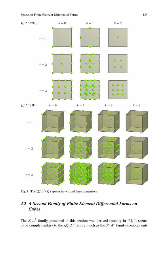
Diagrams for these elements in two and three dimensions are shown in Fig. 4. Thespace Q−

r Λ0(Th) is the standard Qr finite element subspace of H 1(Ω) and the spaceQ−

r Λn(Th) is the discontinuous Qr−1 subspace of L2(Ω). The space Q−r Λ1(Th)

goes back to Raviart and Thomas [20] in two dimensions, and the Q−r Λ1(Th) and

Q−r Λ2(Th) were given by Nédélec in [18]. The spaces with r held fixed combine to

create a finite element de Rham subcomplex,

Q−r Λ0(Th)

d−→Q−r Λ1(Th)

d−→ · · · d−→ Q−r Λn(Th),

and the degrees of freedom determine commuting projections.Recently, Cockburn and Qiu [12] have published a different family of finite el-

ement spaces in two and three dimensions, that seems to be related to these. Theybegin with the complex formed by the full spaces QrΛ

k , which lie between Q−r Λk

and Q−r+1Λ

k . That complex (which was discussed in [19]) does not admit commut-ing projections. Cockburn and Qiu define a small space of bubble functions that canbe added to each of the spaces so that the resulting spaces remain inside Q−

r+1Λk

but also form a de Rham subcomplex (with constant r) which admits commutingprojections.

Spaces of Finite Element Differential Forms 135

Fig. 4 The Q−r Λk(Th) spaces in two and three dimensions

4.2 A Second Family of Finite Element Differential Forms onCubes

The SrΛk family presented in this section was derived recently in [3]. It seems

to be complementary to the Q−r Λk family much as the PrΛ

k family complements

136 D.N. Arnold

the P−r Λk family. To describe the new family we require some notation. A k-form

monomial in n variables is the product of an ordinary monomial and a simple alter-nator:

m = (x1)α1 · · · (xn

)αn dxσ1 ∧ · · · ∧ dxσk ,

where α is a multi-index and σ ∈ Σ(k,n). We define the degree of m to be thepolynomial degree of its coefficient: degm = ∑

i αi . The linear degree of m is morecomplicated:

ldegm = #{i | αi = 1, αi /∈ {σ1, . . . , σk}

},

that is, the number of variables that enter the coefficient linearly, not counting thevariables that enter the alternator. For example, if m = x1x2(x3)5 dx1, then degm =7, ldegm = 1.

We now define the space of shape functions we shall use for k-forms on an n-dimensional box, T . Viewing monomial forms as differential forms on T , we defineHr,lΛ

k(T ) ⊂ HrΛk(T ) to be the span of all monomial k-forms m such that degm =

r and ldegm ≥ l. Using this definition and the Koszul differential, we then define

JrΛk(T ) =

∑

l≥1

κHr+l−1,lΛk+1(T ) ⊂ Pr+n−k−1Λ

k(T ).

Finally, we define the shape functions on T by

SrΛk(T ) = PrΛ

k(T ) +JrΛk(T ) + dJr+1Λ

k−1(T ),

defined for all r ≥ 1, 0 ≤ k ≤ n.As the definition of the shape functions takes a while to absorb, we describe the

spaces in more elementary terms in the case of three dimensions.

• The space SrΛ0, the polynomial shape functions for the H 1 space, consists of

all polynomials u with superlinear degree sdegu ≤ r . The superlinear degree ofa monomial is its degree ignoring any variable that enters to the first power, andthe superlinear degree of a polynomial is the maximum over its monomials. Thecriterion sdegu ≤ r was introduced in [2] to generalize the serendipity elementsfrom 2 to n-dimensions.

• The space SrΛ1, the shape functions for the H(curl) space, consists of vector

fields of the form(v1, v2, v3) + (

x2x3(w2 − w3), x3x1(w3 − w1), x1x2(w1 − w2)) + gradu,

with polynomials vi , wi , and u for which degvi ≤ r , degwi ≤ r − 1, sdegu ≤r + 1, and wi is independent of the variable xi .

• The H(div) space uses shape functions SrΛ2, which are of the form

(v1, v2, v3) + curl

(x2x3(w2 − w3), x3x1(w3 − w1), x1x2(w1 − w2)),

with degvi ≤ r , degwi ≤ r , and wi independent of the variable xi .

Spaces of Finite Element Differential Forms 137

Fig. 5 The SrΛk(Th) spaces in two and three dimensions

• Finally the L2 space SrΛ3 simply coincides with Pr .

In [3] we establish the following properties of these spaces (in any dimension):

• degree property: PrΛk(I n) ⊂ SrΛ

k(In) ⊂ Pr+n−kΛk(In);

• inclusion property: SrΛk(I n) ⊂ Sr+1Λ

k(In);

138 D.N. Arnold

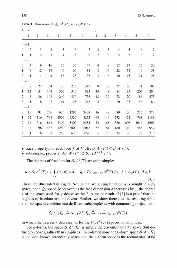
Table 1 Dimension of Q−r Λk(In) and SrΛ

k(In)

k r r

1 2 3 4 5 6 1 2 3 4 5 6

n = 1

0 2 3 4 5 6 7 2 3 4 5 6 7

1 1 2 3 4 5 6 2 3 4 5 6 7

n = 2

0 4 9 16 25 36 49 4 8 12 17 23 30

1 4 12 24 40 60 84 8 14 22 32 44 58

2 1 4 9 16 25 36 3 6 10 15 21 28

n = 3

0 8 27 64 125 216 343 8 20 32 50 74 105

1 12 54 144 300 540 882 24 48 84 135 204 294

2 6 36 108 240 450 756 18 39 72 120 186 273

3 1 8 27 64 125 216 4 10 20 35 56 84

n = 4

0 16 81 256 625 1296 2401 16 48 80 136 216 328

1 32 216 768 2000 4320 8232 64 144 272 472 768 1188

2 24 216 864 2400 5400 10 584 72 168 336 606 1014 1602

3 8 96 432 1280 3000 6048 32 84 180 340 588 952

4 1 16 81 256 625 1296 5 15 35 70 126 210

• trace property: for each face f of I n, trf SrΛk(In) ⊂ SrΛ

k(f );• subcomplex property: dSrΛ

k(I n) ⊂ Sr−1Λk+1(I n).

The degrees of freedom for SrΛk(T ) are quite simple:

u ∈ SrΛk(T ) →

∫

f

(trf u) ∧ q, q ∈Pr−2(d−k)Λd−k(f ), f ∈ �d(T ), d ≥ k.

(4.1)These are illustrated in Fig. 5. Notice that weighting function q is sought in a Ps

space, not a Qs space. Moreover, as the face dimension d increases by 1, the degrees of the space used for q decreases by 2. A major result of [3] is a proof that thedegrees of freedom are unisolvent. Further, we show there that the resulting finiteelement spaces combine into de Rham subcomplexes with commuting projections:

SrΛ0(Th)

d−→ Sr−1Λ1(Th)

d−→ · · · d−→ Sr−nΛn(Th),

in which the degrees r decrease, as for the PrΛK(Th) spaces on simplices.

For n-forms, the space SrΛn(Th) is simply the discontinuous Pr space (but de-

fined on boxes, rather than simplices). In 2-dimensions, the 0-form space SrΛ0(Th)

is the well-known serendipity space, and the 1-form space is the rectangular BDM

Spaces of Finite Element Differential Forms 139

space defined in [10]. Hence these spaces were all known in 2 dimensions. How-ever, in 3 and more dimensions they were not. The 0-form space is the appropriategeneralization of the serendipity space to higher dimensions, a space first defined in2011 [2]. The space SrΛ

2 in 3-D is, we believe, the correct analogue of the BDMelements to cubical meshes. It has the same degrees of freedom as the space in [9]but the shape functions have better symmetry properties. For 1-forms in 3-D, SrΛ

1

is a finite element discretization of H(curl). To the best of our knowledge, neitherthe degrees of freedom nor the shape functions for this space had been proposed pre-viously. Finally, we note that the dimension of S−

r Λk(T ) tends to be much smallerthan that of Q−

r Λk(T ), especially for r large, as can be observed in Table 1.

References

1. Arnold, D.N.: Differential complexes and numerical stability. In: Proceedings of the Inter-national Congress of Mathematicians, vol. I, Beijing, 2002, pp. 137–157. Higher EducationPress, Beijing (2002). MR MR1989182 (2004h:65115)

2. Arnold, D.N., Awanou, G.: The serendipity family of finite elements. Found. Comput. Math.11(3), 337–344 (2011). doi:10.1007/s10208-011-9087-3

3. Arnold, D.N., Awanou, G.: Finite element differential forms on cubical meshes. Preprint(2012). URL: http://arxiv.org/pdf/1204.2595

4. Arnold, D.N., Boffi, D., Bonizzoni, F.: Approximation by tensor product finite element differ-ential forms (2012, in preparation)

5. Arnold, D.N., Falk, R.S., Winther, R.: Finite element exterior calculus, homological tech-niques, and applications. Acta Numer. 15, 1–155 (2006). MR MR2269741 (2007j:58002)

6. Arnold, D.N., Falk, R.S., Winther, R.: Finite element exterior calculus: from Hodge theory tonumerical stability. Bull. Am. Math. Soc. 42(2), 281–354 (2010)

7. Baker, G.A.: Combinatorial Laplacians and Sullivan-Whitney forms. In: Differential Geome-try, College Park, MD, 1981/1982. Progr. Math., vol. 32, pp. 1–33. Birkhäuser, Boston (1983).MR MR702525 (84m:58005)

8. Bossavit, A.: Whitney forms: a class of finite elements for three-dimensional computations inelectromagnetism. IEEE Trans. Magn. 135(Part A), 493–500 (1988)

9. Brezzi, F., Douglas, J. Jr., Durán, R., Fortin, M.: Mixed finite elements for second order ellipticproblems in three variables. Numer. Math. 51, 237–250 (1987). MR MR890035 (88f:65190)

10. Brezzi, F., Douglas, J. Jr., Marini, L.D.: Two families of mixed finite elements for second orderelliptic problems. Numer. Math. 47, 217–235 (1985). MR MR799685 (87g:65133)

11. Ciarlet, P.G.: The Finite Element Method for Elliptic Problems. North-Holland, Amsterdam(1978). MR MR0520174 (58 #25001)

12. Cockburn, B., Qiu, W.: Commuting diagrams for the TNT elements on cubes. Math. Comput.(2012, to appear)

13. Dodziuk, J.: Finite-difference approach to the Hodge theory of harmonic forms. Am. J. Math.98(1), 79–104 (1976). MR MR0407872 (53 #11642)

14. Dodziuk, J., Patodi, V.K.: Riemannian structures and triangulations of manifolds. J. IndianMath. Soc. (N.S.) 40(1–4), 1–52 (1976). MR MR0488179 (58 #7742)

15. Hiptmair, R.: Canonical construction of finite elements. Math. Comput. 68, 1325–1346(1999). MR MR1665954 (2000b:65214)

16. Kotiuga, P.R.: Hodge decompositions and computational electromagnetics. PhD in ElectricalEngineering, McGill University (1984)

17. Müller, W.: Analytic torsion and R-torsion of Riemannian manifolds. Adv. Math. 28(3), 233–305 (1978). MR MR498252 (80j:58065b)

140 D.N. Arnold

18. Nédélec, J.-C.: Mixed finite elements in R3. Numer. Math. 35, 315–341 (1980). MRMR592160 (81k:65125)

19. Nédélec, J.-C.: A new family of mixed finite elements in R3. Numer. Math. 50, 57–81 (1986).MR MR864305 (88e:65145)

20. Raviart, P.-A., Thomas, J.-M.: A mixed finite element method for 2nd order elliptic prob-lems. In: Mathematical Aspects of Finite Element Methods, Proc. Conf., Consiglio Naz.delle Ricerche (C.N.R.), Rome, 1975, pp. 292–315. Lecture Notes in Mathematics, vol. 606.Springer, Berlin (1977). MR MR0483555 (58 #3547)

21. Robin, J.W., Salamon, D.A.: Introduction to differential topology (2011). Lecture notesfor a course at ETH Zürich. URL: http://www.math.ethz.ch/~salamon/PREPRINTS/difftop.pdf

22. Sullivan, D.: Differential forms and the topology of manifolds. In: Manifolds—Tokyo 1973,Proc. Internat. Conf., Tokyo, 1973, pp. 37–49. Univ. Tokyo Press, Tokyo (1975). MRMR0370611 (51 #6838)

23. Sullivan, D.: Infinitesimal computations in topology. Publ. Math. IHÉS 1977(47), 269–331(1978). MR MR0646078 (58 #31119)

24. Whitney, H.: Geometric Integration Theory. Princeton University Press, Princeton (1957). MRMR0087148 (19,309c)