Spaceborne Receiver Design for Scatterometric GNSS...
245
Spaceborne Receiver Design for Scatterometric GNSS Reflectometry Philip Jales Submitted for the Degree of Doctor of Philosophy from the University of Surrey Surrey Space Centre Faculty of Engineering and Physical Science University of Surrey Guildford, Surrey, GU2 7XH, UK July 2012
Transcript of Spaceborne Receiver Design for Scatterometric GNSS...

Spaceborne Receiver Design for Scatterometric GNSS Reflectometry
Philip Jales
Submitted for the Degree of Doctor of Philosophy
from the University of Surrey
Surrey Space Centre Faculty of Engineering and Physical Science
University of Surrey Guildford, Surrey, GU2 7XH, UK
July 2012


1
Spaceborne Receiver Design for Scatterometric GNSS Reflectometry
Global Navigation Satellite System-Reflectometry (GNSS-R) is an innovative technique for
remote sensing. It uses reflected signals from the navigation constellations to determine
properties of the Earth’s surface. The primary focus of this work is the remote sensing of the
ocean by measurement of surface roughness. The most significant unresolved challenge in
spaceborne GNSS-R is to verify the accuracy of surface roughness measurements. Existing
remote sensing techniques have typically relied on extensive data-sets to validate satellite
measurements with the ground truth. This thesis provides a receiver design for collection of
the required validation data-sets which can then form part of an operational system for surface
roughness measurement.
New receiver approaches were investigated through the design of a software receiver to post-
process existing data from the GNSS-R experiment on the UK-DMC satellite. This forms the
reflections into Delay-Doppler Maps (DDMs) from which the surface roughness can be
determined. The software receiver improves on existing implementations by targeting all
available specular reflections using open-loop tracking. A new approach called Stare
processing is analysed, which controls the receiver to remain focused at a fixed point on the
Earth’s surface as the satellites move. This improves the surface resolution over using the full
DDM. Additionally it is shown to be a viable approach for surface roughness measurement
through a scattering model and the first demonstration on data collected from space.
GNSS-R research has primarily focused on the established GPS navigation system. This
research extends the measurement concept to the new Galileo GNSS. A receiver that can
target multiple GNSS constellations will allow greater remote sensing coverage. The primary
differences between Galileo and GPS are analysed and an approach is developed leading to
the first spaceborne demonstration of Galileo-like signals for remote sensing.
The system design for the GNSS-R receiver presented in this thesis was carried out in the
context of Surrey Satellite Technology Ltd developing a GNSS navigation receiver called the
SGR-ReSI, to be launched on the UK Technology Demonstrations Satellite TDS-1. The
critical areas identified in the GNSS-R system design were implemented and tested on this
receiver. The design overcomes the challenging constraints of GNSS-R in a small satellite
platform: principally the mass, power and data downlink capacity. To achieve these, on-board
data compression was developed through real-time DDM processing and reflection tracking.
An algorithm for real-time DDM processing within the mass and power constraints was
designed and demonstrated within the receiver and combined with open-loop reflection
tracking. A ground-based test set-up was developed to test the design on existing spaceborne
data, from the UK-DMC experiment, before the TDS-1 satellite launch.

2
Acknowledgements
This thesis would not have been possible without the valuable guidance and help of a number
of individuals. I would like to express my gratitude for the support of my supervisor Dr. Craig
Underwood. Additionally I would like to thank my industrial supervisor Dr. Martin Unwin
who provided invaluable guidance and practical knowledge.
This research has been supported by the EPSRC, Surrey Satellite Technology Limited and
Surrey Space Centre. I would like to express my sincere gratitude to all my colleagues at
SSTL and SSC for their help and friendship. In particular I would like to thank the GNSS
Receivers Team at SSTL for their help in the design and realisation of the real-time GNSS-R
processor and providing inspiration and motivation. My thanks also go to Scott Gleason who
collected many of the data sets used in this thesis from the UK-DMC GNSS-R experiment.
Finally my greatest thanks go to my family for their love and support over the past years and
my wife Sarah for her patience, encouragement and unfailing support throughout.

3
Table of Contents
Acknowledgements ................................................................................................................... 2
Table of Contents ...................................................................................................................... 3
Chapter 1: Introduction ....................................................................................................... 16
1.1. CASE PhD Studentship at SSTL .............................................................................. 16
1.2. The Motivation for Ocean Remote Sensing with GNSS .......................................... 17
1.3. The Present State of Global Navigation Satellite Systems ....................................... 19
1.4. Bistatic Radar ........................................................................................................... 20
1.5. GNSS Remote sensing.............................................................................................. 21
1.6. Thesis Goals ............................................................................................................. 22
1.7. Outline of Thesis ...................................................................................................... 22
Chapter 2: Background ....................................................................................................... 24
2.1. GNSS-R from Space ................................................................................................. 26
2.2. Bistatic Radar Equation ............................................................................................ 27
2.2.1. GNSS Signal Structure ...................................................................................... 28
2.2.2. Delay and Doppler Spreading ........................................................................... 33
2.2.3. Scattering Models .............................................................................................. 34
2.2.4. Surface Model ................................................................................................... 38
2.3. GNSS-R Receiver ..................................................................................................... 41
2.3.1. Mapping the DDM to the Surface ..................................................................... 45
2.3.2. DDM Sensitivity to Ocean Roughness .............................................................. 46
2.3.3. Coherence Time ................................................................................................ 48
2.3.4. Coherent and Non-Coherent Integration ........................................................... 51
2.3.5. Measurement Inversion ..................................................................................... 52
2.4. UK-DMC and On-Going Work at Surrey ................................................................ 53
2.4.1. SGR-ReSI and TechDemoSat-1 ........................................................................ 55
2.5. Instruments in Development ..................................................................................... 57
2.5.1. ESA: PARIS ...................................................................................................... 57
2.5.2. NASA / JPL ....................................................................................................... 58
2.5.3. UPC, Barcelona ................................................................................................. 59
2.5.4. IEEC .................................................................................................................. 59
2.5.5. Starlab ................................................................................................................ 60
2.5.6. Further Context ................................................................................................. 61
Chapter 3: System Design ................................................................................................... 62
3.1. System Design Concept ............................................................................................ 63
3.2. UK-DMC Parameters ............................................................................................... 64
3.3. Scattering Geometry ................................................................................................. 67
3.4. Receiver Altitude ...................................................................................................... 71
3.5. Modernised and Wide-Band GNSS Signals ............................................................. 74
3.6. Antenna Gain and Coverage ..................................................................................... 81
3.7. Discussion ................................................................................................................. 84
Chapter 4: Tools and Techniques for GNSS-R ................................................................... 86
4.1. MATLAB Software Receiver System Description .................................................. 87
4.2. Reflection Open-loop Tracking ................................................................................ 88

4
4.3. Reprocessing UK-DMC Data ................................................................................... 92
4.4. Calculation of the Specular Point Location .............................................................. 93
4.4.1. Spherical Earth Approximation ......................................................................... 97
4.4.2. Quasi-Spherical Earth ....................................................................................... 98
4.4.3. Ellipsoidal Earth .............................................................................................. 101
4.4.4. Optimisation in Polar Coordinates .................................................................. 107
4.4.5. Error Sources ................................................................................................... 110
4.4.6. Verification on UK-DMC Data ....................................................................... 112
4.4.7. Discussion ....................................................................................................... 115
4.5. Galileo-Reflectometry ............................................................................................ 116
4.5.1. Processing of GIOVE Signals ......................................................................... 117
4.5.2. Signal Combinations ....................................................................................... 122
4.5.3. Coherence Time .............................................................................................. 126
4.5.4. Experimental Verification ............................................................................... 128
4.5.5. Discussion ....................................................................................................... 134
4.6. Stare Processing ...................................................................................................... 135
4.6.1. Stare Geometry ................................................................................................ 136
4.6.2. Scattering Cross Section .................................................................................. 139
4.6.3. Theoretical Model ........................................................................................... 141
4.6.4. The Area Term ................................................................................................ 144
4.6.5. Effective Swath ............................................................................................... 146
4.6.6. Impact On Receiver ......................................................................................... 151
4.6.7. Orbital Results ................................................................................................. 154
4.7. Scattering Cross-Section Measurement .................................................................. 160
4.7.1. Transmitter Terms ........................................................................................... 163
4.7.2. Receiver Terms ............................................................................................... 164
4.7.3. Relative Power Measurement .......................................................................... 165
4.7.4. Power Measurement Through A Coarsely Quantised Analogue To Digital
Converter ........................................................................................................................ 168
4.8. Discussion of the Software Receiver ...................................................................... 176
Chapter 5: Real-Time Processing ..................................................................................... 178
5.1. Motivation .............................................................................................................. 178
5.2. Processing Split Between Satellite and Ground ..................................................... 180
5.2.1. Comparison With a Navigation Receiver “Cold Search” ............................... 182
5.2.2. Sampling Resolution ....................................................................................... 183
5.3. Existing Work ......................................................................................................... 185
5.4. Processing Architecture .......................................................................................... 186
5.5. Time-Domain Techniques ...................................................................................... 188
5.6. Frequency Domain Techniques .............................................................................. 191
5.6.1. Code Correlation in the Frequency Domain ................................................... 192
5.6.2. Doppler Search Using the Frequency Domain ................................................ 195
5.7. DDM Processor Implementation ............................................................................ 201
5.8. Real-Time Tracking ................................................................................................ 205
5.8.1. Real-Time Tracking Implementation .............................................................. 210
5.9. Verification and Demonstration ............................................................................. 212
5.10. Real-time Processing Discussion............................................................................ 215
Chapter 6: Discussion and Conclusions ............................................................................ 217
6.1. Contributions .......................................................................................................... 217

5
6.2. Future Work ............................................................................................................ 219
6.3. Publications and Presentations ............................................................................... 220
References ............................................................................................................................. 222
Appendix A. Example Software Receiver Output .............................................................. 231
Appendix B. Stare Processing Results from UK-DMC Experiment .................................. 233
Appendix C. DC Bias .......................................................................................................... 235
Appendix D. DDM Processor Implementation ................................................................... 239
Appendix E. Catalogue of UK-DMC data collections ....................................................... 240

6
List of Figures
Figure 1.1 Artists rendering of QuikSCAT (Source http://winds.jpl.nasa.gov) ....................... 18
Figure 2.1 Definitions in GNSS-R sensing .............................................................................. 24
Figure 2.2 Photograph of the sun reflecting off the sea. Region of calm water highlighted by
ellipse ....................................................................................................................................... 25
Figure 2.3 Iso-delay ellipses and iso-Doppler hyperbolas segment the surface ...................... 26
Figure 2.4 Overview of remote sensing geometry of GNSS-R. (overlay of Google Earth
imagery) ................................................................................................................................... 27
Figure 2.5 Normalised auto-correlation function for GPS C/A PRN 1. Left: Full code auto-
correlation. Right: zoom to chip range -10 to +10. .................................................................. 31
Figure 2.6 The ambiguity function for the BPSK, GPS C/A code on L1, using a coherent
integration time of 1ms ............................................................................................................ 32
Figure 2.7 Rayleigh criterion between rough and smooth scattering, dependent on elevation
angle from satellite at 700km altitude ...................................................................................... 35
Figure 2.8 Definitions of scattering in model geometry. Adapted from [Bian 2007] ............. 36
Figure 2.9 Elfouhaily surface mss with wind speed (U10) for a well-developed sea and
showing two incidence angles. ................................................................................................. 40
Figure 2.10 Schematic of down-conversion and sampling architecture used to produce an IF
signal ........................................................................................................................................ 41
Figure 2.11 Delay Doppler Map calculation array, showing recovery of the DDM. ............... 42
Figure 2.12 Delay Doppler map, grid of delay and Doppler. Each pixel’s value represents the
correlation power for that delay and Doppler .......................................................................... 43
Figure 2.13 Delay Doppler map showing two chosen correlator channels .............................. 44
Figure 2.14 Mapping from surface scattering locations to the signal space in the delay-
Doppler map ............................................................................................................................. 45
Figure 2.15 DDM models for a UK-DMC-like geometry, for some of the smoothest (A) and
roughest (B) ocean conditions, where both have the same receiver and transmitter locations to
allow comparison. .................................................................................................................... 47
Figure 2.16 Illustration of the lines of iso-delay and iso-Doppler on the surface, defining the
size of the 1st-iso-range ellipse. (A) Perspective view (B) Plan view of surface. ................... 49
Figure 2.17 Schematic of UK-DMC GNSS-R receiver hardware. Courtesy of SSTL. ........... 54
Figure 2.18 Modifications to the SGR-20 GPS receiver to allow connection to the data-logger.
Courtesy of SSTL. .................................................................................................................... 54
Figure 2.19 SGR-ReSI system diagram. Courtesy of SSTL .................................................... 56
Figure 2.20 Rendering of TechDemoSat-1 in orbit. Courtesy of SSTL. ................................. 56
Figure 2.21 Schematic of TOGA instrument. NASA [Meehan, Esterhuizen, et al. 2007] ...... 59
Figure 2.22 GOLD-RTR receiver. IEEC [Nogues-Correig, Cardellach Gali, et al. 2007] ...... 60
Figure 3.1 Image of UK-DMC showing the GNSS-R antenna ................................................ 65
Figure 3.2 UK-DMC antenna pattern cuts through the maximum gain, measured before
satellite launch. Showing: (A) the elevation cut. (B) the azimuth cut. The half-power beam
width is marked. ....................................................................................................................... 65
Figure 3.3 Reflection detectability for variation of antenna gain for all UK-DMC data
collections, based on 10 seconds incoherent accumulation. .................................................... 66
Figure 3.4 Diagram showing the labelling of quantities [adapted from Hajj, Zuffada, et al.
2002] ......................................................................................................................................... 69
Figure 3.5 Change in area of the first iso-range ellipse with receiver altitude......................... 72
Figure 3.6 Free space path loss in comparison to 650km altitude ........................................... 73

7
Figure 3.7 Reflection power change of 1st iso-range ellipse due to altitude ............................ 73
Figure 3.8 Band usage of the modernised GPS (courtesy of [Weiler 2009]) ........................... 74
Figure 3.9 Band usage of Galileo (courtesy of [Weiler 2009]) ................................................ 74
Figure 3.10 Width of the 1st iso-range ellipse, showing the surface resolutions for the L1 C/A
and E5a/b signals. ..................................................................................................................... 76
Figure 3.11 Surface area of 1st iso-range ellipse with varying bandwidth signals .................. 76
Figure 3.12 Reflection power compared to GPS L1 for varying bandwidth signals ............... 77
Figure 3.13 Plan view onto Earth surface of two limiting case geometries for coherence time
determination. ........................................................................................................................... 78
Figure 3.14 Coherence time for L1 and E5 signals with angle of specular point from
receiver’s nadir. (650 km altitude receiver) ............................................................................. 79
Figure 3.15 Processing gain change through exploiting coherence time increase in comparison
to those of 2 MHz bandwidth. Wavelength fixed at 0.19 m. ................................................... 80
Figure 3.16 Reflection power compared to GPS L1 for varying bandwidth signals. Including
processing gain from variation in coherence time. .................................................................. 80
Figure 3.17 Geometry of angles subtended at receiver translated into transmitter position .... 82
Figure 3.18 Average number of simultaneous reflections for nadir pointing antenna with
range of antenna HPBW ........................................................................................................... 83
Figure 3.19 Number of simultaneous reflections with antenna gain for parabolic antenna ..... 84
Figure 4.1 Software receiver schematic representation of the GNSS-R processing flow. ....... 87
Figure 4.2 Timing of signal propagation for direct and reflected rays .................................... 89
Figure 4.3 All UK-DMC data collections where the specular point reflection power is above a
detection threshold ................................................................................................................... 93
Figure 4.4 Difference between direct and reflected path lengths ............................................. 95
Figure 4.5 Monte-Carlo elevation distribution for 10,000 runs. .............................................. 97
Figure 4.6 Spherical Earth approximation. (A) Distance from solution |S – S*| (B) Distance
error in path 𝑹𝑺𝑻 ...................................................................................................................... 98
Figure 4.7 Quasi-spherical approximation for determining the specular point location ......... 99
Figure 4.8 Path-length sensitivity to surface height (Left) and horizontal displacement (Right)
.................................................................................................................................................. 99
Figure 4.9 Quasi-spherical Earth approximation (A) Distance from solution 𝑺 − 𝑺 ∗ (B)
Distance error in path RST ..................................................................................................... 101
Figure 4.10 Convergence using constrained steepest descent................................................ 103
Figure 4.11 Convergence of constrained steepest descent to determine specular point location
K = 1,000,000 ......................................................................................................................... 103
Figure 4.12 Constrained steepest descent, convergence error. Earth flattening exaggerated 104
Figure 4.13 Convergence of improved constrained steepest descent. Using K = 1,000,000 . 105
Figure 4.14 Number of iterations required to converge to E < 3*10-6
................................... 106
Figure 4.15 Specular point calculation geometry using polar coordinates (reproduced from
[Garrison, Komjathy, et al. 2002] ) ........................................................................................ 107
Figure 4.16 Equatorial latitude convergence in polar coordinates ......................................... 109
Figure 4.17 High latitude convergence in polar coordinate system ....................................... 109
Figure 4.18 Minimisation in polar coordinates: Number of iterations until convergence step
size within |fn - fn+1| < 10-9
m .................................................................................................. 110
Figure 4.19 Diagram showing the relationship between geoid and reference ellipsoid (1)
Undisturbed ocean. (2) Reference ellipsoid (3) Local plumb line (4) Continent (5) Geoid.
[Reproduced from Wikipedia:Geoid 2011] ............................................................................ 110

8
Figure 4.20 Deviation of the EGM96 geoid from the WGS-84 reference ellipsoid
[Reproduced from MathWorks Mapping Toolbox 2012] ...................................................... 111
Figure 4.21 Correlation functions generated with open-loop tracking on the direct signal, as
received through the zenith and nadir antennas ..................................................................... 112
Figure 4.22 Power DDM of 'PUR3' data set PRN 1, open-loop tracking aligned to (0,0). 1000
incoherent accumulations of 1 ms coherent correlations ....................................................... 113
Figure 4.23 Determining the open-loop tracking error . Delay cut of the DDM. Upper)
processed delay range. Lower) Zoom in around tracking point showing tracking error ....... 113
Figure 4.24 Convolution of the surface impulse response with the signal ACF .................... 114
Figure 4.25 Histogram of open-loop tracking error in UK-DMC data sets. Using ellipsoidal
Earth model ............................................................................................................................ 115
Figure 4.26 BOC(1,1) modulation components. PRN code c(t) and subcarrier sc(t) ............ 119
Figure 4.27 Correlation function of the BOC(1,1) (blue) and BPSK (red) spreading codes. 119
Figure 4.28 Incoherent addition of the E1B and E1C components ........................................ 122
Figure 4.29 Coherent addition of E1B and E1C components ................................................ 123
Figure 4.30 Coherent addition of E1B and E1C components, with post correlation delay line
................................................................................................................................................ 124
Figure 4.31 Histograms of noise only (n), and signal + noise (s+n). Showing separate E1B and
E1C correlation magnitude compared to L1B+L1C coherent addition ................................. 126
Figure 4.32 Histograms of noise only (n), and signal + noise (s+n). Comparing |E1B|+|E1C| to
|E1B+E1C| .............................................................................................................................. 126
Figure 4.33 The incoming signal is split into 4 sub-blocks and zero-padded. ....................... 127
Figure 4.34 A simulation of the BOC(1,1) frequency spectrum in red, filtered by the IF SAW
filter in the receiver, forming the blue spectrum .................................................................... 129
Figure 4.35 The BOC(1,1) correlation function in red following filtering by the IF SAW filter,
forms the smoothed blue ACF ............................................................................................... 129
Figure 4.36 Enlarged view of the filtered BOC(1,1) ACF ..................................................... 130
Figure 4.37 The geometry of UK-DMC and its receiver antenna pattern in red durign the
Arafua sea data collection. ..................................................................................................... 130
Figure 4.38 The received secondary code, correlated with the published code ..................... 131
Figure 4.39 E1B data, d(t), correlated with the 10 bit SYNC word and circled at 1 second
intervals .................................................................................................................................. 132
Figure 4.40 DDM and delay map of the ocean reflected signal from GIOVE-A, 1 second
integration. Arafura Sea 04/11/2007 ...................................................................................... 132
Figure 4.41 DDM and delay map of the ocean reflected signal from GIOVE-A, 8 second
integration. Arafura Sea 04/11/2007 ...................................................................................... 133
Figure 4.42 Iso-delay and iso-Doppler lines on the surface. There is an ambiguity between the
left and right side of the dotted line ........................................................................................ 136
Figure 4.43 GNSS-R Stare processing geometry at three different times. Left diagram earliest
in time and right diagram being latest. ................................................................................... 138
Figure 4.44 DDM with stare point delay and Doppler plotted. (R12 dataset, PRN15) ......... 138
Figure 4.45 Time series plan view of surface during part of stare observation of point P at
(0,0). The receiver starts above the specular point and as it moves leftwards, the specular
point also moves from (0,0) to the left. (Column A) Projection of the AF magnitude on
surface. (Column B) The iso-Doppler and iso-Delay lines. ................................................... 140
Figure 4.46 Model of the scattering cross-section profile during a Stare processing
measurement for a range of ocean conditions. (A) shows the absolute 𝝈0 (B) shows the
normalised 𝝈0. ........................................................................................................................ 143

9
Figure 4.47 (Above) Area integral, A, with distance of Stare point from specular point.
(Below Left) Plan view of the selected surface for |P-S| = 0 km and (Below Right) |P-S| = 115
km. Where P is at (0,0). ......................................................................................................... 145
Figure 4.48 Time series plan view of surface, whilst staring at fixed point P at (0,0). Views at
4 second intervals through simulated UK-DMC orbit. (Column A) Projection of the AF
magnitude on surface. (Column B) The iso-Doppler and iso-Delay lines ............................. 147
Figure 4.49 Geometry used to parameterise specular point location for investigation of Stare
processing resolution .............................................................................................................. 149
Figure 4.50 Size of the signal AF projected onto the surface, for range of specular point
locations.(A) shows the selected surface area. (B) shows the half-power width of the AF. .. 150
Figure 4.51 Delay and Doppler difference between TSR and TPR paths over time. P=S at 100
seconds. .................................................................................................................................. 151
Figure 4.52 Stare processing surface measurements at surface points P0, P1, P2… Each ray
corresponds to a single 𝝈0 measurement for the corresponding Pi......................................... 152
Figure 4.53 Correspondence between surface and DDM areas ............................................. 153
Figure 4.54 Ground resolution from Stare processing, showing 10 measurements ............... 154
Figure 4.55 Stare processing measurement from a UK-DMC dataset taken over the ocean.
Specular point and stare point coincide at 9 seconds. (Dataset R44, PRN 10). ..................... 156
Figure 4.56 Stare observation using UK-DMC data collection R44, PRN 10. Three stare
points (A), (B) and (C) are processed .................................................................................... 158
Figure 4.57 Scale picture of the scattering geometry of receiver in low-Earth orbit and the
transmitter in medium-Earth-orbit ......................................................................................... 161
Figure 4.58 Angle between direct and reflected rays from transmitter. (A) shows maximal
difference angle, and (B) the extreme cases. .......................................................................... 163
Figure 4.59 Angle between direct and specular rays from the transmitter. Dotted line
corresponds to Earth limb. ..................................................................................................... 164
Figure 4.60 Schematic of receiver architecture to perform relative calibration using a cross-
over switch ............................................................................................................................. 166
Figure 4.61 ADC quantisation input and output values for different ADC accuracies. Output
scaled to the range [–1, +1] .................................................................................................... 169
Figure 4.62 Quantisation model ............................................................................................. 169
Figure 4.63 GNSS signal component power measured across a range of input noise power.
Input noise power is signal and noise combined power P (Equation 4.56) ........................... 172
Figure 4.64 Output noise power from ADC given range of input noise power. Input power is
ratio (expressed in dB) of the ideal RMS noise power for each of the n-bit ADCs. .............. 173
Figure 4.65 Change in measured GNSS component power with measured output power .... 174
Figure 5.1 SSTL supplied 5 multispectral ground-imagery satellites for the RapidEye
constellation in 2008. (Courtesy: Surrey Satellite Technology) ............................................ 179
Figure 5.2 SGR-ReSI flight model ......................................................................................... 180
Figure 5.3 Processing chain for producing surface measurement from DDM of reflected
signal. ..................................................................................................................................... 181
Figure 5.4 A UK-DMC reflection processed using the software receiver. Colour scale is
chosen to provide a measure of reflection detectability. Processing as described in Section 4.1.
................................................................................................................................................ 183
Figure 5.5 FPGA resource utilisation on Virtex-4 series devices from Xilinx for circuits that
perform A*B=C and A+B=C. The number of bits used to represent A and B is varied to show
the influence of the calculation precision. .............................................................................. 187
Figure 5.6 Forming a single pixel in the DDM, using time domain approach ....................... 188

10
Figure 5.7 Correlator array, sized 3x3, made up from multiple discrete, time-domain
correlators ............................................................................................................................... 189
Figure 5.8 Correlator array resource sharing the incoherent accumulations .......................... 190
Figure 5.9 Number of LUTs used for discrete correlator array. (A) The horizontal surface
indicates the capacity of the reference Xilinx Virtex-4 SX35 chip of 30,700 LUTs. (B) Shows
the view of this surface, showing the DDM processor dimensions that would fit within the
device. .................................................................................................................................... 191
Figure 5.10 Computing the DDM by individual pixel computation (A), or by transformation
into the frequency domain for calculation of lines of constant Doppler (B) or delay (C) lines
simultaneously. ....................................................................................................................... 192
Figure 5.11 Frequency domain correlation (adapted from [Pany 2010] ) .............................. 194
Figure 5.12 Computation of DDM row through process of downconversion, modulation
removal followed by spectrum estimation ............................................................................. 197
Figure 5.13 Moving average filter .......................................................................................... 198
Figure 5.14 Frequency response of 1st order CIC filter, with D = 512 and fs=16367 kHz.
Green band is pass-band requirement of 10 kHz. .................................................................. 199
Figure 5.15 Running average filter followed by decimation(A). Rearrangement to reduce
sample rate of comb section (B) ............................................................................................. 200
Figure 5.16 The CIC filter response from Figure 5.14, showing the new sampled bandwidth,
fs,out/2. Signal energy in the red bands will then be aliased into the green pass-band. ........... 200
Figure 5.17 Aliasing into the pass-band (green) .................................................................... 201
Figure 5.18 Block diagram of the real-time DDM processor as implemented in hardware .. 202
Figure 5.19 A result from real-time DDM output from playback of UK-DMC dataset R44
PRN10 direct signal and 500 ms integration .......................................................................... 204
Figure 5.20 Cuts through the real-time DDM processor output compared to software receive.
Data set R44, PRN10 (A) Doppler map. (B) Delay map ....................................................... 204
Figure 5.21 Flow of information from direct signal tracking to reflection tracking, via the
navigation solution ................................................................................................................. 206
Figure 5.22 Interpolation of geometrical state. ...................................................................... 207
Figure 5.23 Extrapolation of geometrical state ...................................................................... 207
Figure 5.24 From orbital simulation: Direct and reflected path lengths ................................ 208
Figure 5.25 From orbital simulation: (A) Rate of change of path length, (B) Rate of path
length acceleration .................................................................................................................. 209
Figure 5.26 From orbital simulation: (A) Rate of change of path length, (B) Rate of path
length acceleration .................................................................................................................. 210
Figure 5.27 Structure and timing of the software control for open-loop tracking ................. 211
Figure 5.28 Schematic of the data flow for the verification of the real-time GNSS-R system
................................................................................................................................................ 213
Figure 5.29 Monitoring the real-time tracking within SGR-PC3 software ............................ 214
11
List of Tables
Table 3.1 GNSS system signal specification ........................................................................... 75
Table 4.1 Comparison of GPS and GIOVE signals centred on 1.57542GHz. (Excluding
secured signals) ...................................................................................................................... 120
Table 4.2 State table for the E1B and E1C modulation states ............................................... 125
Table 4.3 GPS and GIOVE-A minimum received power comparison .................................. 134
Table 4.4 Calibration accuracy achievable due to ADC ........................................................ 174
Table 4.5 Surface reflectance error estimates ........................................................................ 175
Table 5.1 Maximum loss with different sampling resolutions in Doppler dimension ........... 184
Table 5.2 Maximum loss with different sampling resolutions in delay dimension ............... 184
Table 5.3 Reflectometry DDM processor requirements compared to navigation cold search.
................................................................................................................................................ 185
Table 5.4 Resource utilisation for discrete correlator components ........................................ 189

12
List of Symbols
𝑖 - Incidence angle of reflection. Angle between incident ray and surface normal.
휀 - Grazing angle of reflection. Angle between incident ray and surface tangent.
𝜌𝐷, 𝜌𝐷 - Pseudo-range of direct and reflected paths respectively
𝑹 - Receiver position vector
𝑻 - Transmitter position vector
𝑺 - Specular point position vector
𝑷 - Position vector of fixed point on the surface of the Earth
𝝆 - Position vector of point on Earth’s surface
𝜃 - Angle of off pointing from receiver nadir to specular point
𝜃𝑇 - Angle of off pointing from transmitter nadir to specular point
Δ𝜃𝑇 - Difference in angle between the specular point and the receiver from the
transmitter
|𝑹𝑺⃗⃗⃗⃗ ⃗| - Distance from receiver to specular point
|𝑻𝑺⃗⃗⃗⃗ ⃗| - Distance from transmitter to specular point
|𝑻𝑹⃗⃗ ⃗⃗ ⃗| - Distance from transmitter to receiver
|𝑹| - Orbital radius of the receiver
|𝑻| - Orbital radius of the transmitter
Θ - Angle between receiver and transmitter Earth radials
𝛼 - Angle between the transmitter Earth radial and the specular point Earth radial
𝑓𝑐 - Code chip frequency of GNSS signal
𝑓𝐿 - Carrier frequency of the GNSS signal
𝑓𝐼 Carrier frequency of the GNSS signal following down-conversion in receiver,
named the Intermediate Frequency (IF).
𝑓𝑠 - Sample frequency
𝑐 - Speed of light
𝜎0 - Scattering cross-section per unit area
𝜆 - Radio wave-length
𝐴 - Signal amplitude
𝑃 - Signal power
𝑇𝑖𝑛𝑐𝑜ℎ - Incoherent accumulation period
𝑀 - Number of incoherent accumulations
𝑇𝑐𝑜ℎ - Coherent integration time
𝑇𝑐 - Chip period
𝑇𝐷 - Data bit period
𝑁𝑐 - Number of chips in periodic PRN code
𝑵 - Earth surface normal
𝑎 - Earth semi-major axis in WGS-84 ellipsoid
𝑏 - Earth semi-minor axis in WGS-84 ellipsoid
𝑠(𝑡) - GNSS signal as transmitted
𝑢(𝑡) - GNSS signal as received
𝑤 - Correlation integration result
𝑛(𝑡) - Noise at input to receiver

13
𝑛𝑊 - Post correlation noise
𝑃𝑅𝑥𝑅 - Signal power incident on the receiver from the reflection component
𝑃𝑅𝑥𝐷 - Signal power incident on the receiver from the direct signal
𝑃�̂�, 𝑃�̂� - Power measured by the receiver of the reflected and directed signal
respectively
𝐺𝑇𝑥 - Gain of GNSS transmitter antenna
𝐺𝑅𝑥𝐷 - Gain of receiver antenna for the direct signal ray
𝐺𝑅𝑥𝑅 - Gain of receiver antenna for the reflected signal ray
𝑃𝑇𝑥 - Transmitted power
𝐺 - Receiver gain in amplifier stages
𝐺𝑉 - Receiver gain in automatic gain control / variable gain amplifier
𝐺𝑞 - Quantisation gain (from loss in analogue to digital conversion)
𝑇𝑅 - Receiver noise temperature
𝑇𝐴𝐷, 𝑇𝐴
𝑅 - Noise temperature from receiver antennas (Direct and Reflection)
KD, KR - Free space path loss terms grouped together for the direct and reflected rays.
𝑡 - Time
𝜒(Δ𝑡, Δ𝑓) - Ambiguity Function (AF) of GNSS signal, with delay offset 𝛥𝑡, and
frequency offset 𝛥𝑓
𝛬(𝛥𝑡) - Auto-correlation function of GNSS signal with delay offset 𝛥𝑡
𝑡’ - Receiver replica time delay
𝑓’ - Receiver replica carrier frequency
𝑓𝐷 - Difference in carrier frequency due to Doppler shift
𝒗𝑻 - Transmitter velocity vector
𝒗𝑹 - Receiver velocity vector
𝜔 - Orbital angular velocity of satellite
𝑊 - Bandwidth
Γ - Absolute signal to noise ratio as measured by the receiver
Γ0 - Processed signal to noise ratio
𝑁𝑑 - Number of delay pixels in delay Doppler map
𝑁𝑓 - Number of frequency pixels in delay Doppler map
𝑁𝑅 - Number of reflection PRN codes computed by DDM processor

14
List of Abbreviations
ACF - Auto Correlation Function
AF - Ambiguity Function
AGC - Automatic Gain Control
ASIC - Application Specific Integrated Circuit
BOC - Binary Offset Carrier
BPSK - Binary Phase Shift-Keyed
C/A - Course / Acquisition GPS signal
CDMA - Code Division Multiple Access
CIC - Cascaded Integrator Comb
DCO - Digitally Controlled Oscillator
DDM - Delay Doppler Map
DDR2 - Double Data Rate 2 (memory interface standard)
DFT - Discrete Fourier Transform
ECEF - Earth-Centred, Earth-Fixed frame of reference
FDMA - Frequency Division Multiple Access
FFT - Fast Fourier Transform
FIFO - First-In First-Out
FPGA - Field Programmable Gate Array
GIOVE - Galileo In Orbit Validation Experiment
GIOVE - Galileo In Orbit Validation Element satellite
GLONASS - The Russian Global Navigation Satellite System: Globalnaya
Navigatsionnaya Sputnikovaya Sistema
GNSS - Global Navigation Satellite System
GNSS-R - GNSS-Reflectometry
GO - Geometric Optics
GPS - Global Positioning System
GPS - Global Positioning System
HDL - Hardware Description Language
IF - Intermediate Frequency
IFFT - Inverse Fast Fourier Transform
KA - Kirchhoff Approximation
Kibits/s - 210 bits per second
L1 - A carrier frequency of GPS and Galileo systems at 1.57542 GHz
L2 - A carrier frequency of GPS system at 1.2276 GHz
L5 - A carrier frequency of GPS and Galileo in the protected aeronautical band
LNA - Low Noise Amplifier
LEO - Low Earth Orbit
LHCP - Left-Hand Circularly Polarised
LUT - Look Up Table
Mcps - Mega chips per second
MEO - Medium Earth Orbit
Mibits/s - 220 bits per second - 210 bits per second
mss - Mean Square Slope
MUX - Multiplexer
NCO - Numerically Controlled Oscillator
PDF - Probability Density Function

15
PLL - Phase Locked Loop
PO - Physical Optics
PRN - Pseudo Random Noise / Identifier for GPS satellite
RF - Radio Frequency
RHCP - Right-Hand Circularly Polarised
RO - Radio Occultation
Rx - Receiver
SGR - Space GNSS Receiver
SGR-ReSI - Space GNSS Receiver Remote Sensing Instrument
SNR - Signal to Noise Ratio
SP - Specular Point
SSTL - Surrey Satellite Technology Ltd.
TDS-1 - TechDemoSat-1
Tx - GNSS transmitter
UK-DMC - United Kingdom- Disaster Monitoring Constellation satellite
VHDL - VHSIC Hardware Description Language
Z-V - Zavorotny-Voronovich model

16
Chapter 1: Introduction
This chapter introduces the groups that have invested and contributed to this research. A brief
history of the contributing parties is provided to give the context within which the project
developed. Following this, a brief introduction is given, on the present state of satellite
navigation and radar remote sensing. Finally a short description of the content in the
subsequent chapters is given.
1.1. CASE PhD Studentship at SSTL
The CASE PhD is a studentship created by the Electrical and Physical Sciences Research
Council (EPSRC) to promote collaboration between industry and academia. The CASE
studentships provide funding for PhD studentships where a business takes the lead in
arranging a project which combines the shared research goals of both industrial and academic
partners. A bias towards more practical work and development tend to result from this
structure than in a traditional PhD.
The industrial partner in this CASE studentship is Surrey Satellite Technology Limited
(SSTL). SSTL was formed as a spin-off company from the University of Surrey in 1985.
SSTL has since been involved in over 31 satellite missions and become a world-leader in
supplying satellites platforms. SSTL has specialised in applying the technological
developments in telecommunications and consumer electronics to making small and highly
capable optical imaging satellites. SSTL manufactures its own range of GNSS receivers,
which are operated on-board its own satellites and supplied externally as sub-systems. SSTL
has provided GPS receivers for satellite communication constellations such as for
ORBCOMM Generation 2 with over 60 receivers supplied. SSTL have pioneered a number
of novel space applications with their GNSS receivers [SSTL 2011].
SSTL has been working on the European Navigation project, Galileo [Benedicto, Dinwiddy,
et al. 2000]. SSTL constructed and still operates the first satellite in this project, called
GIOVE-A, which was launched in December 2005 [Gatti, Garutti, et al. 2001]. This satellite
was a particular achievement for SSTL considering their size at the time. Since then SSTL
has been contracted to provide the navigation payloads for the next 22 Galileo satellites. The
Introduction
17
components that generate the navigation signals are being procured from external suppliers
but the process has brought a lot of GNSS signal experience into the company.
The academic partner for this PhD is Surrey Space Centre (SSC), part of the Faculty of
Engineering and Physical Sciences at the University of Surrey. The department was the
birthplace of SSTL and works in all areas of space research. There are a number of research
collaborations between the two organisations, including projects on radar remote sensing.
Surrey has had a background in GNSS remote sensing with the launch of a GNSS-R
experimental receiver on the UK-DMC satellite in 2003. This was followed by two PhDs in
the area, during which, [Gleason 2006] principally demonstrated a link between sea state and
the properties of the reflected GNSS signal using data collections from UK-DMC. The ocean
surface models were then improved by [Bian 2007].
1.2. The Motivation for Ocean Remote Sensing with GNSS
Measurements of the wind over the ocean surface are needed for weather forecasting and
climate monitoring. The only routine global measurements are provided by satellite-borne
scatterometers for observation of ocean winds and altimeters for ocean waves. The ocean
winds are of particular importance due to their influence on shipping, coastal communities,
ocean currents and the climate.
Accurate marine weather predictions have far reaching consequences to safety of life and
commercial interests. Satellite measurements of ocean roughness are used for storm detection
to determine the location, direction, structure and strength of storms for early warning of
coastal communities. Knowledge of the wind behaviour enables the routing of ships to avoid
heavy seas that may cause vessel damage or increased fuel consumption.
The prediction and tracking of climate anomalies such as El Niño are largely dependent on
the synoptic measurements from ocean wind scatterometers [Liu 2005].
The sea surface is the boundary between the atmosphere and the ocean and has an important
influence on climate. The interactions at the ocean-atmosphere interface regulate the gas, heat
and momentum transfer between the two masses. In addition, the surface wind stresses are an
important driver of ocean circulation [Marshall & Plumb 2008, chap.10]. An understanding
of the sea surface is therefore a critical factor in understanding and modelling climate change.
18
The measurement of ocean winds is reliant on satellite missions as Michael Freilich, director
of the Earth Science division at NASA Headquarters puts it, “Seventy percent of the Earth's
surface is covered by the ocean, and we actually have very few direct measurements of winds
over the ocean, except for satellites such as QuikSCAT” [Spaceflight Now 2009]. However,
these satellites are a considerable investment and there has historically been a difficulty in
transitioning from technology demonstration missions to operational services. The
climatologist community in particular find continuity of measurements vital in minimising
measurement biases in these long-term comparisons.
Concurrent with the time of this thesis the operating scatterometers were limited to the
American Seawinds on QuikSCAT [Tsai, Spencer, et al. 2000], European ASCAT on MetOp
[Figa-Saldana, Wilson, et al. 2002] and Indian SCAT on Oceansat-2 [Parmar, Arora, et al.
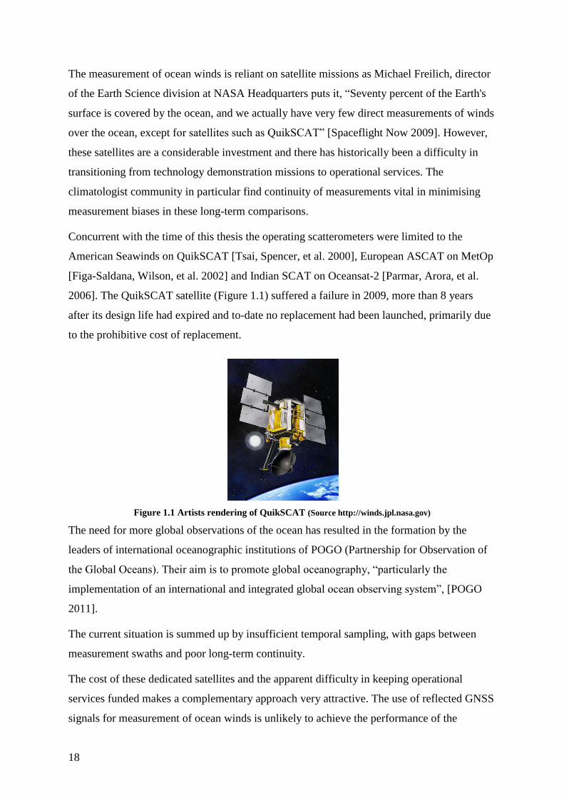
2006]. The QuikSCAT satellite (Figure 1.1) suffered a failure in 2009, more than 8 years
after its design life had expired and to-date no replacement had been launched, primarily due
to the prohibitive cost of replacement.
Figure 1.1 Artists rendering of QuikSCAT (Source http://winds.jpl.nasa.gov)
The need for more global observations of the ocean has resulted in the formation by the
leaders of international oceanographic institutions of POGO (Partnership for Observation of
the Global Oceans). Their aim is to promote global oceanography, “particularly the
implementation of an international and integrated global ocean observing system”, [POGO
2011].
The current situation is summed up by insufficient temporal sampling, with gaps between
measurement swaths and poor long-term continuity.
The cost of these dedicated satellites and the apparent difficulty in keeping operational
services funded makes a complementary approach very attractive. The use of reflected GNSS
signals for measurement of ocean winds is unlikely to achieve the performance of the

Introduction
19
dedicated instruments, as the transmitter properties are tuned for their navigation purpose
rather than for remote sensing. Specifically, the transmission frequencies available with
GNSS limit accuracy of the ionospheric correction to the propagation delay [Fu & Cazenave
2000], the signal bandwidth limits the ranging resolution and the transmission power affects
the statistics of the measurements [Gleason, Gommenginger, et al. 2010]. GNSS-R provides a
promising complimentary role to dedicated systems for filling coverage gaps, increasing
temporal sampling and providing continuity of measurement.
1.3. The Present State of Global Navigation Satellite Systems
To set the background, an overview of the status of the GNSS systems will be given, as this
gives an indication of how the Earth’s surface is being covered with signals from GNSS
satellites and therefore of the opportunities available.
The work done for this thesis was undertaken during a time of significant change in satellite
navigation. The two heritage systems GPS and GLONASS [Polischuk, Kozlov, et al. 2002]
were starting to be significantly improved, a development probably driven by Europe’s heavy
investment in their own independent system, Galileo. A fourth GNSS, a Chinese based
solution has also emerged during the time of this research. The two new systems and the two
heritage systems were all actively improving satellite navigation with the introduction of new
signals and concepts. This global investment in GNSS is producing, as a by-product, a
growing opportunity for remote sensing.
The basic architecture for GPS was approved by the Department of Defence in 1973 [Misra
& Enge 2006, chap.1]. The constellation then reached its operational level of 24 satellites in
1994. During this time the system transitioned from a military service to a dual-use system,
with continuation of the civilian signals protected by law. It was agreed in 2000 that GPS
would be modernised with two additional civil signals, including a new wide bandwidth
signal.
The Russian GLONASS fell into decline in the 1990s; however a reprioritisation has meant
that the system is in resurgence and has again reached a fully-operational constellation. The
operational concept is similar to GPS except the satellites broadcast the same code on a
number of different frequencies to prevent interference. This is a frequency division multiple
access scheme (FDMA) rather than code division multiple access (CDMA), which is used in
GPS. The GLONASS constellation is undergoing modernisation with a new generation of

20
satellites, GLONASS-K, which includes a CDMA signal for civilian applications. The first
GLONASS-K satellite was launched in February 2011 and the modernised service is
proposed to be operational by 2020.
The European Union is progressing with its Galileo GNSS. At the time of this project two
test satellites GIOVE-A and GIOVE-B had been operating in orbit for a number of years and
two of the four In-Orbit Validation (IOV) satellites had been launched. In this context there is
a considerable research interest in the new signal characteristics that are being provided in
this new system.
The Chinese system, BeiDou (Compass) Navigation Satellite System has launched 10
operational satellites as of December 2011. This provides an operational service over China
and is planned to extend into global coverage by 2020. The signal designs were being
finalised only late in the stages of this research. This is a growing system and has many
compatible features to the other GNSS operators, such as modulation type, frequency and
bandwidth [China Satellite Navigation Project Center 2009].
GPS is currently the most widely used GNSS; most of the work in this thesis will refer to
GPS although the work is largely applicable to any GNSS. In specific cases the differences
between systems are highlighted. As the other systems followed GPS, there are certain
conventions, such as the fundamental basis of the clock at 1.023 MHz which is repeated in all
the systems. There is the prospect of four GNSS constellations of between 24 and 32
satellites each and additionally regional overlay services such as WAAS and EGNOS. The
combination creates a large number of sources for a GNSS-R receiver to use in sampling the
Earth’s surface.
1.4. Bistatic Radar
Radars are used for detecting, ranging and measuring characteristics of targets. The most
common radar configuration is monostatic, when the transmitter and receiver are co-located
and they often share the same antenna. In bistatic radar the transmitter and receiver are not
co-located. The receiver may be cooperating with the transmitter, in some bistatic radars, or
operating completely independently and passively using a signal of opportunity.
From the radar surveillance and target identification fields the return from extended surfaces
such as the ocean is known as the clutter and is normally a nuisance return that interferes with
the detection of targets [Skolnik 2008]. However it is actually this clutter response that is of
Introduction
21
interest for ocean remote sensing. Many of the models of ocean surface scattering are based
on the clutter models firstly developed for monostatic radar and then extended to bistatic.
A review of bistatic scattering models and scattering cross-section measurement campaigns
for various surfaces can be found in [Willis, Griffiths, et al. 2007, chap.9]
1.5. GNSS Remote sensing
GNSS has already had considerable impact on remote sensing techniques. The most
successful application can be said to be in Radio Occultation (RO), which is a remote sensing
technique used to measure the physical properties of the planet’s atmosphere [Liou 2010].
This is carried out through detection of a change in the radio signal as it refracts through the
atmosphere. The magnitude of the refraction depends on the gradients of atmospheric density
and water vapour. In the neutral atmosphere information on the atmosphere’s temperature,
pressure and water vapour can be derived. These measurements have had a large impact in
meteorology and are incorporated into numerical weather prediction such as [ECMWF 2007],
which combines about 50,000 soundings per day from multiple satellite constellations
including COSMIC (Constellation Observing System for Meteorology, Ionosphere, and
Climate) [Liou, Pavelyev, et al. 2007] and the GRAS instrument on MetOp-A [Loiselet,
Stricker, et al. 2000].
In contrast to the maturity of atmospheric sensing using GNSS, measurement of the Earth’s
surface is relatively immature despite being proposed as a scatterometric measurement tool
before GPS had even reached its operational capability, [Hall & Cordey 1988]. Once GPS
had become operational in the mid-1990s, further attention was given to applications other
than navigation such as the first published detailed proposal in [Martin-Neira 1993], which
contains a description of an overall system for using these transmitters of opportunity to
characterise the Earth’s surface. Since then a number of research organisations have worked
on theoretical descriptions and experimental realisations such as the early aircraft
experiments by [Garrison, Katzberg, et al. 1998].
Although GNSS remote sensing could be considered as a multi-static system, (multi-
transmitter, one or more receivers) in practice the link margin precludes sensing from
anywhere other than around the point of mirror like reflection (specular point). The location
of one transmitter’s specular point will not typically coincide with that of another transmitter

22
due to their physical separation. This means that only one transmitter is effectively used at a
time and so is normally considered to be a bistatic arrangement.
At this stage GNSS-R has the principal unresolved challenge to verify the accuracy of the
surface characterisation. Existing satellite remote sensing techniques have typically relied on
considerable data sets from the satellite instrument to compare to ground truth and thus build
empirical retrieval models.
The UK’s Technology Strategy Board (TSB) and the South East England Development
Agency (SEEDA) have together provided funding for a technology demonstration satellite
called TechDemoSat-1 (TDS-1). As UK organisations are currently experiencing a huge cost
barrier to a first flight demonstration for satellite equipment, this satellite mission aims to
address this issue by providing an in-orbit test-bed for UK technology. The results of this
thesis contribute to the development a GNSS-R instrument that is scheduled for launch on
TDS-1 during early 2013.
1.6. Thesis Goals
There is a pressing need for more observations of the ocean surface. GNSS-Reflectometry
has shown considerable promise in the measurement of the ocean roughness and is
anticipated to provide a complimentary service to the existing monostatic scatterometers and
ocean altimeters.
The aim of this research is to provide a method of gaining more GNSS-R data to build
empirical models for retrieval of a measure of ocean roughness. This thesis contributes to the
goal of an operational ocean roughness GNSS-R sensor through a system design of a
spaceborne receiver, demonstration of remote sensing techniques by post-processing real data
in a software receiver and a real-time implementation in a receiver that is scheduled for
launch on the UK funded TechDemoSat-1.
1.7. Outline of Thesis
The thesis consists of 6 chapters, with the following content:
Chapter 2 describes the concept of surface measurement with GNSS-R, introduces the
theoretical model of the scattering mechanisms and the receiver processing operations.

Introduction
23
Following this the GNSS-R receivers being proposed or developed at other organisations are
described with their relations to the goals of this research.
Chapter 3 presents a system design trade-off analysis for a remote sensing instrument that is
suited to the constraints of a small satellite platform. A model of the scattering around the
specular point is used to investigate key aspects of the system design of the GNSS-R receiver.
Chapter 4 details the development of a software receiver test-bed, which is then used for
verifying several new GNSS-R techniques. The gathering of the verification and validation
data needed to invert spaceborne GNSS-R observations to ocean roughness measurements
presents the greatest challenge at the time of this research. The post-processing techniques
developed in this chapter work towards a spaceborne GNSS-R sensor that can collect the
required data. The software receiver is used to verify the tracking algorithms for the reflected
signals. Then the software receiver is used to demonstrate new techniques for utilising the
Galileo signals for improved temporal sampling of the Earth’s surface. A new processing
approach called Stare processing is introduced and validated on real data. Finally a method
for calibration of the surface reflectance is developed that overcomes the limitations of using
commercially available radio-frequency components.
Chapter 5 addresses the principle challenges for a satellite based GNSS-R sensor: the
required downlink bandwidth, power and mass. The most flexible approach for a spaceborne
receiver is to downlink to the ground the raw sampled signals, although this produces a data-
rate which is incompatible with the capabilities of a small satellite platform, so on-board
processing is required. An on-board processing approach has been developed that reduces the
data-rate by an order of magnitude. This real-time processing is developed and tested on
simulated reflected signals. To target the on-board processing to the location of the
reflections a real-time tracking approach is developed.
Chapter 6 states the contributions made during this thesis to the advancement of GNSS-R.
Following this, suggestions are made for future research into areas covered by this research.
24
Chapter 2: Background
In oceanographic research the two main applications of GNSS-R sensing are altimetry for
surface height measurement and scatterometry for sea surface roughness measurement.
Considering that GNSS-R is a technique with important differences from the existing radar
altimeter, scatterometer and synthetic aperture radar techniques, this chapter starts with an
attempt to provide the reader with a way of visualising the measurement approach. The
chapter then follows from the simple visualisation to a more in-depth introduction to the
scattering geometry, the bistatic radar equation, scattering model and the quantities
measurable by the receiver. The chapter concludes with a description of the GNSS-R
instruments in development and how this research project extends the field and opens new
opportunities in remote sensing with the design of a new GNSS-R receiver.
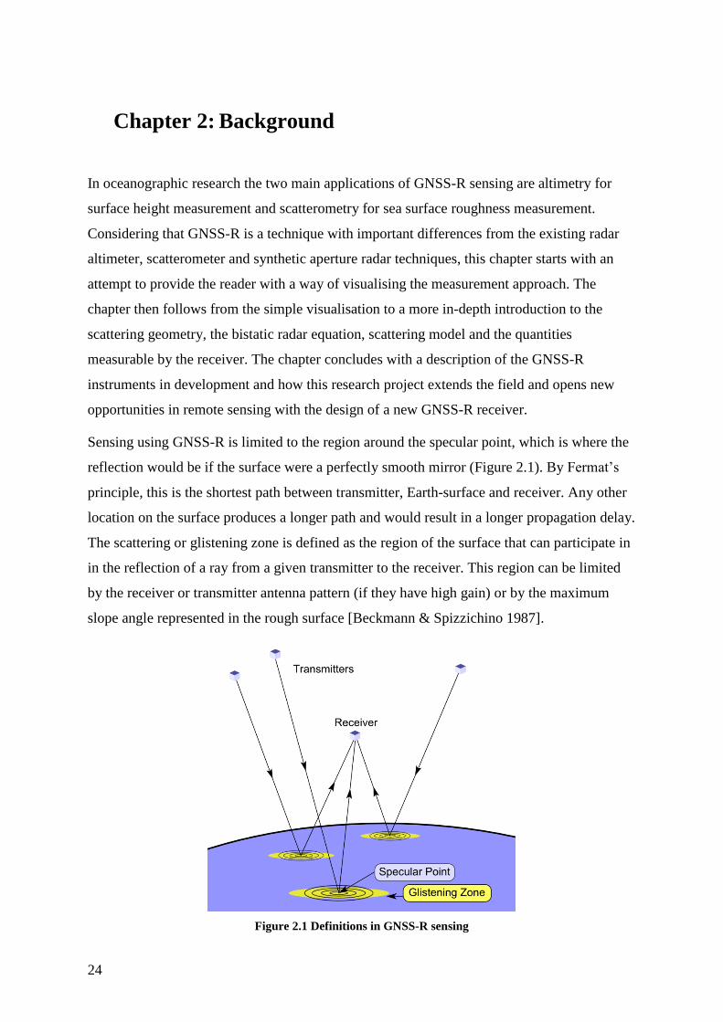
Sensing using GNSS-R is limited to the region around the specular point, which is where the
reflection would be if the surface were a perfectly smooth mirror (Figure 2.1). By Fermat’s
principle, this is the shortest path between transmitter, Earth-surface and receiver. Any other
location on the surface produces a longer path and would result in a longer propagation delay.
The scattering or glistening zone is defined as the region of the surface that can participate in
in the reflection of a ray from a given transmitter to the receiver. This region can be limited
by the receiver or transmitter antenna pattern (if they have high gain) or by the maximum
slope angle represented in the rough surface [Beckmann & Spizzichino 1987].
Figure 2.1 Definitions in GNSS-R sensing

Background
25
To help explain the principal of using scattered GNSS signals for remote sensing of the ocean
it can be helpful to visualize a more familiar scenario, sunlight reflecting from the water. The
reflection from a calm, smooth, pond will be considerably different from that off a stormy
and hence rough sea. Figure 2.2 shows a photograph where the apparent scattering area varies
around a band of calmer water. The calm water is smoother resulting in a reduction of the
scattering zone size. From the extent of the scattering zone the roughness of the surface can
be inferred by a GNSS-R receiver.
Figure 2.2 Photograph of the sun reflecting off the sea. Region of calm water highlighted by ellipse
[from Chapron and Ruffini, GNSS-R workshop, Barcelona 2002]
Unlike in sunlight reflections a receiver will see multiple scattering zones, one for each
GNSS transmitter. The receiver can distinguish between signals using the GNSS transmitter
signal modulation. The inherent difficulty with using the GNSS transmitters is the lack of
control or repeatability of the reflection geometry.
In practice the analogy of sun-light reflections is useful for visualisation of the scattering,
however microwave radar is not a camera-like imaging technique. A GNSS-R receiver,
instead, uses observations of the scattering zone differentiated by signal travel time (reception
delay) and Doppler shift.
The specular point is the shortest path from transmitter to Earth to receiver, around which
surface points with equal propagation delay form iso-delay rings, Figure 2.3. If the Earth is
approximated as a plane surface around the specular point then the iso-delay rings are
ellipses. This shape forms as the surface plane intersects the receiver-transmitter ellipsoid
(the ellipsoid having receiver and transmitter at its foci).

26
The movement of receiver and transmitter relative to the surface cause the propagation delay
to change, causing a Doppler shift on the reflected signal. On the surface, points with equal
rate-of-change of the path delay form iso-Doppler lines, Figure 2.3. If the receiver velocity
dominates (as is the case for a low-Earth-orbit receiver) then the surface of iso-Doppler is a
cone with axis aligned to the receiver velocity. The intersections of the cone and Earth
surface plane results in a hyperbola for each iso-Doppler contour. The iso-range and iso-
Doppler lines deviate from these planar functions if the Earth is modelled more precisely as
spherical or ellipsoidal. The mapping of surface to delay and Doppler is not one-to-one so
imaging is not straightforward.
Figure 2.3 Iso-delay ellipses and iso-Doppler hyperbolas segment the surface
2.1. GNSS-R from Space
Traditional monostatic altimeters are limited to looking in the nadir direction and then
collecting one track of surface height observations. A GNSS-R sensor in low Earth orbit
would be able to track multiple reflections simultaneously and build up coverage enabling
significantly greater temporal and spatial resolution.
In comparison to conventional scatterometers, the sensing geometry is more complex as the
measurement points appear over the ocean not as a swath, or a single point, but as a number

Background
27
of points that travel along the surface with the receiver motion, as illustrated in Figure 2.4.
For a low-Earth-orbit receiver the motion of the specular points is dominated by the motion
of the fast-moving receiver, rather than the high altitude, slower moving, GNSS transmitters.
Figure 2.4 Overview of remote sensing geometry of GNSS-R. (overlay of Google Earth imagery)
Now the foundations of GNSS-R will be introduced, starting with the model for the reflected
signals using the bistatic radar equation. Each part of this is then separated down to form an
understanding of GNSS-R.
2.2. Bistatic Radar Equation
To gain insight into the applications of GNSS-Reflectometry a model of the scattering is
needed. A model is introduced here using the bistatic radar equation, which is followed by
defining the structure of the GNSS signals, and then the scattering is modelled from a rough
surface, finally a model of the ocean surface is provided.
The model uses the Geometric Optics (GO) limit of the Kirchhoff Approximation (KA) for
the short-wave, bistatic, rough-surface scattering problem [Bass & Fuks 1977; Beckmann &
Spizzichino 1987; Voronovich 1999]. This approach is to segment the surface into discrete
scattering facets or planes. Then the received signal is modelled as the sum of returns from
this very large number of independent scatterers. This approach requires that the surface is a
statistically rough surface.
The expectation of the reflected signal power ⟨𝑃𝑅𝑥𝑅 ⟩ arriving at the receiver can be modelled
by the integration over the surface, 𝝆,

28
⟨𝑃𝑅𝑥
𝑅 ⟩ = 𝑇𝑐𝑜ℎ2
λ2 ∙ 𝑃𝑇𝑥
(4π)3∬
𝐺𝑇𝑥(𝝆) ∙ 𝐺𝑅𝑥𝑅 (𝝆) ∙ 𝜎0(𝝆) ∙ 𝜒2(𝑡 − 𝑡′(𝝆), 𝑓 − 𝑓′(𝝆))
|𝑹𝝆⃗⃗ ⃗⃗ ⃗|2∙ |𝑻𝝆⃗⃗⃗⃗ ⃗|
2 d2𝝆
𝝆
(2.1)
This sums the signal responses over all the surface facets, with the contribution of each one
depending on its surface location 𝝆.
The terms are as follows:
𝑇𝑐𝑜ℎ Coherent integration time
𝜆 Radio wavelength
𝑃𝑇𝑥 Transmitted power
𝐺𝑇𝑥 Transmitter antenna gain
𝐺𝑅𝑥𝑅 Receiver’s antenna gain for the reflected ray from 𝝆
𝜎0 Bistatic scattering cross-section normalised to a unit of surface area
𝑹 Position vector of the receiver
𝑻 Position vector of the transmitter
|𝑹𝝆⃗⃗ ⃗⃗ ⃗| Distance from the receiver to 𝝆
|𝑻𝝆⃗⃗⃗⃗ ⃗| Distance from the transmitter to 𝝆
The function, 𝜒 is the Ambiguity Function (AF) of the signal which results from the matched
filtering of the signal for the delay and Doppler frequency of the reflection and depends on
the properties of the signal. The delay and Doppler are represented as 𝑡′and 𝑓′ respectively.
The received power is dependent on the physical properties of the surface through the surface
bistatic radar cross-section (RCS). This abstraction is the area of a hypothetical surface that
isotropically reradiates the incident power and produces the same measurement at the
receiver. The term used here is the bistatic normalised radar cross-section (NRCS), 𝜎0, which
is the RCS per unit surface area.
It can be seen that the main contribution of the integral comes from the intersection of several
spatial zones. These are the transmitter and receiver antenna gains, 𝐺𝑇𝑥 and 𝐺𝑅𝑥𝑅 , the
glistening zone defined by the scattering cross-section 𝜎0 and the zone selected by the GNSS
signals’ ambiguity function 𝜒2 selected by both the delay and frequency. The following
sections further define each of these zones.
2.2.1. GNSS Signal Structure
The properties of the GNSS signal enter the radar equation through the ambiguity function 𝜒.
This will now be defined through exploring the structure of the GNSS signals. A thorough

Background
29
reference for GNSS receiver fundamentals and signal structures is provided by [Kaplan 2006]
and [Tsui 2005].
The signal model for an unperturbed direct signal as transmitted by a GNSS transmitter will
be expressed as a carrier modulated by spreading code 𝑐(𝑡) and data 𝑑(𝑡),
𝑠(𝑡) = √𝑃 𝑑(𝑡) 𝑐(𝑡) exp(𝑗2𝜋𝑓𝑡) (2.2)
It has transmission power 𝑃, and carrier frequency 𝑓. The modulating code 𝑐(𝑡) is a Pseudo-
Random Noise (PRN) sequence 𝑐(𝑡) ∈ (−1,1), so that the modulation is Binary Phase Shift
Keyed (BPSK). In Section 4.5 this will be extended to another class of GNSS modulation,
although for much of the research in this thesis the discussion will relate to the GPS Coarse
Acquisition (C/A) code, which uses BPSK.
The C/A code is a 𝑁𝑐 = 1023 chip long sequence from the Gold code family [Gold 1967].
Each bit or ‘chip’ of the code is 𝑇𝑐 = 1/1.023 μs long so has a chip rate of 1.023 Mcps. The
term 𝑑(𝑡) is the navigation data signal, which is transmitted at a rate of 50 Hz. The
navigation data contains the information necessary for a navigation receiver to compute
position, velocity and time solutions.
Following propagation of the signal to the receiver, the GNSS component, 𝑠(𝑡), is modified
by the channel, becoming the signal as received, 𝑢(𝑡). This is buried in thermal additive
thermal noise 𝑛(𝑡) and has remaining amplitude 𝐴 after attenuations from free-space path
loss, antenna gains, atmospheric losses and other linear scaling. The signal additionally
experiences a time delay,𝜏, and Doppler shift 𝑓𝐷. This results in the GNSS signal component
from equation (2.2) having the general form once received,
𝑢(𝑡) = 𝐴 𝑑(𝑡 − 𝜏) 𝑐(𝑡 − 𝜏) exp(𝑗2𝜋(𝑓 + 𝑓𝐷)𝑡) + 𝑛(𝑡) (2.3)
For the receiver to extract the signal back out of the noise, the signal is frequency translated,
through multiplication by the local oscillator, exp(−𝑗2𝜋𝑓′𝑡 + 𝜙). Then it is cross-correlated
with an internally generated replica, 𝑐(𝑡 − 𝑡′). The cross-correlation result 𝑤 is taken for the
replica with the general time misalignment of 𝑡′, carrier frequency 𝑓′, and a carrier phase
difference of 𝜙,

30
𝑤(𝑡′, 𝑓′) =
𝐴
𝑇𝑐𝑜ℎ∫ [exp(−𝑗2𝜋𝑓′𝑡 + 𝜙) 𝑐(𝑡 − 𝑡′)
𝑇𝑐𝑜ℎ
0
( 𝑑(𝑡 − 𝜏) 𝑐(𝑡 − 𝜏) exp(𝑗2𝜋(𝑓 + 𝑓𝐷)𝑡) + 𝑛(𝑡)) ]𝑑𝑡
(2.4)
There are now two symbols for the time and frequency offsets: the propagation offsets, 𝜏, 𝑓𝐷,
and the offsets of the internal replica signal, 𝑡′, 𝑓′. This integration retains the signal phase so
is called the coherent integration over the time period, 𝑇𝑐𝑜ℎ. The complex formulation is used
here, whereas in a physical receiver the real and imaginary parts are conventionally called the
I and Q channels. The data symbol changes at low rate, so if replica and signal are aligned
and integrated over a time less than the data bit period, then 𝑑(𝑡) can be taken outside of the
integral. Expanding out the terms, the correlation result is,
𝑤(𝑡′, 𝑓′) =
𝐴 𝑑
𝑇𝑐𝑜ℎ∫ 𝑐(𝑡 − 𝜏)𝑐(𝑡 − 𝑡′) exp(𝑗2𝜋(𝑓 + 𝑓𝐷 − 𝑓′)𝑡 + 𝜙)
𝑇𝑐𝑜ℎ
0
+𝑛(𝑡) exp(𝑗2𝜋𝑓′𝑡) 𝑐(𝑡 − 𝑡′)𝑑𝑡
(2.5)
It is helpful to interpret this as a matched filtering process. The thermal noise component
post-correlation becomes the result of filtering the noise by the frequency response of the
modulation code, 𝑐(𝑡). For convenience the noise component post-correlation will be
redefined as the complex vector 𝑛𝑤. The correlation result then becomes,
𝑤(𝑡′, 𝑓′) =
𝐴 𝑑
𝑇𝑐𝑜ℎ∫ 𝑐(𝑡 − 𝜏)𝑐(𝑡 − 𝑡′) exp( 𝑗2𝜋(𝑓 + 𝑓𝐷 − 𝑓′)𝑡 + 𝜙)
𝑇𝑐𝑜ℎ
0
𝑑𝑡 + 𝑛𝑤 (2.6)
As the modulation code 𝑐(𝑡) is a pseudo random sequence, the expectation of the product
⟨𝑐(𝑡 − 𝜏)𝑐(𝑡 − 𝑡′)⟩ can be considered to be time-invariant with minimal error. The
expectation is no longer a function of time and then can be removed from the integral. This
leads to the result that the code and frequency can be held as independent variables.
𝑤(𝑡′, 𝑓′) =
𝐴 𝑑
𝑇𝑐𝑜ℎ ⟨𝑐(𝑡 − 𝜏)𝑐(𝑡 − 𝑡′)⟩
∫ exp(𝑗2𝜋(𝑓 + 𝑓𝐷 − 𝑓′)𝑡 + 𝜙)𝑇𝑐𝑜ℎ
0
𝑑𝑡 + 𝑛𝑤
(2.7)

Background
31
The expectation ⟨𝑐(𝑡 − 𝜏)𝑐(𝑡 − 𝑡′)⟩ is the auto-correlation function (ACF) of the pseudo-
random code. The form of the ACF can be investigated by setting the propagation delay,
𝜏 = 0, the expectation can be expressed in relation to the time delay of the replica 𝑡′. The
GPS C/A code is well-approximated by the function Λ(𝑡′/𝑇𝑐), which is defined,
⟨𝑐(𝑡)𝑐(𝑡 − 𝑡′)⟩ = Λ(𝑡′) = {
−1/𝑁𝑐, |𝑡′/𝑇𝑐| ≥ 1
1 − |𝑡′/𝑇𝑐|, |𝑡′/𝑇𝑐| < 1
(2.8)
where 𝑇𝑐 is the time period of each PRN code chip. In practice the auto-correlation function
for the set of Gold codes used in for GPS C/A codes are not ideal, exhibiting additional cross
correlation amplitudes of {-1/1023, -65/1023, 63/1023}. Outside of the time-aligned interval
the cross-correlation function is almost zero, except due to the odd number of chips it reduces
down to −1/𝑁𝑐. The true auto-correlation of GPS C/A code is calculated for GPS PRN 2 and
shown in Figure 2.5.
Figure 2.5 Normalised auto-correlation function for GPS C/A PRN 1. Left: Full code auto-correlation.
Right: zoom to chip range -10 to +10.
Due to the relatively small errors from the cross correlations, the idealisation Λ is often used
in GNSS-R. The idealised ACF is now substituted into the correlation result of equation
(2.7). The signal propagation delay, 𝜏, causing the time offset of the ACF function,
𝑤(𝑡′, 𝑓′) =
𝐴 𝑑
𝑇𝑐𝑜ℎΛ(𝜏 − 𝑡′)∫ exp(𝑗2𝜋(𝑓 + 𝑓𝐷 − 𝑓′)𝑡 + 𝜙)
𝑇𝑐𝑜ℎ
0
𝑑𝑡 + 𝑛𝑤 (2.9)
-500 0 500-0.2
0
0.2
0.4
0.6
0.8
1
1.2
Time delay [code chips]
Norm
alis
ed a
uto
-corr
ela
tion
-10 -5 0 5 10-0.2
0
0.2
0.4
0.6
0.8
1
1.2
Time delay [code chips]
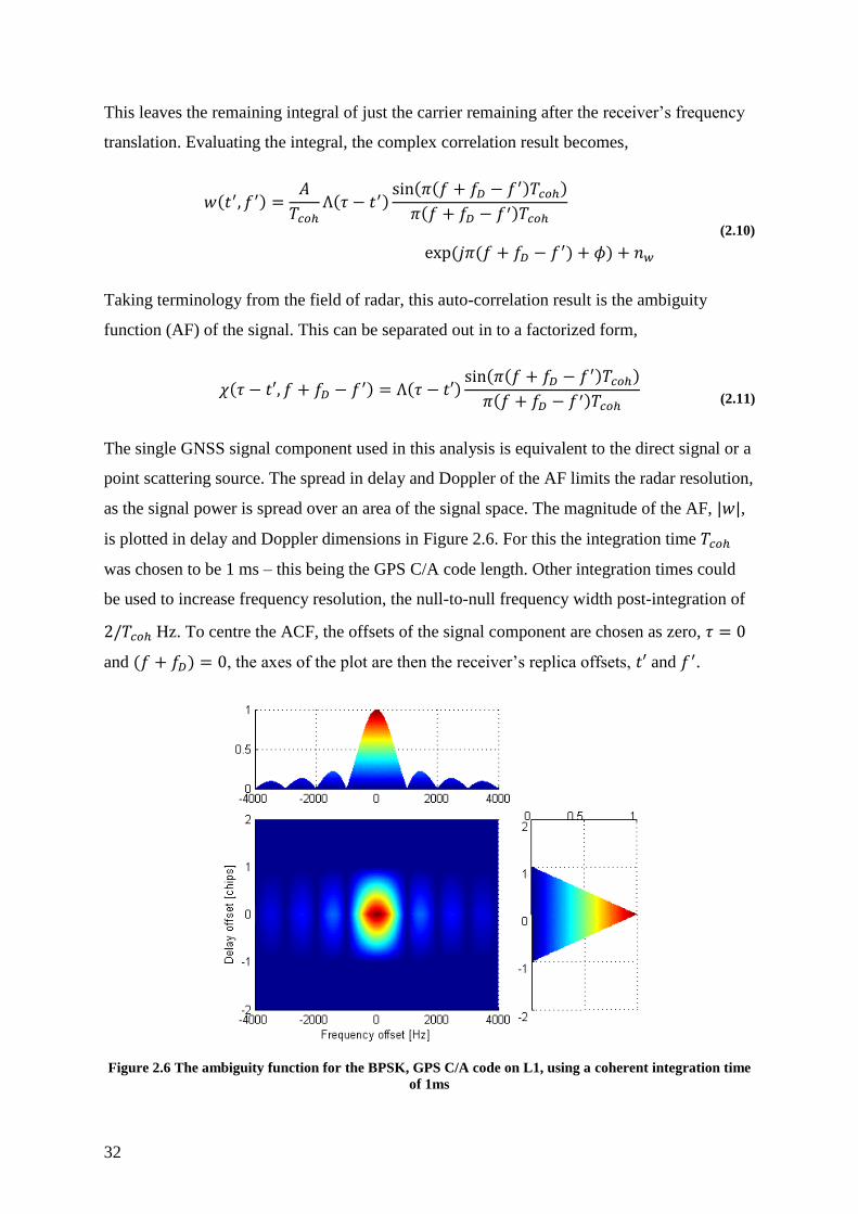
32
This leaves the remaining integral of just the carrier remaining after the receiver’s frequency
translation. Evaluating the integral, the complex correlation result becomes,
𝑤(𝑡′, 𝑓′) =
𝐴
𝑇𝑐𝑜ℎΛ(𝜏 − 𝑡′)
sin(𝜋(𝑓 + 𝑓𝐷 − 𝑓′)𝑇𝑐𝑜ℎ)
𝜋(𝑓 + 𝑓𝐷 − 𝑓′)𝑇𝑐𝑜ℎ
exp(𝑗𝜋(𝑓 + 𝑓𝐷 − 𝑓′) + 𝜙) + 𝑛𝑤
(2.10)
Taking terminology from the field of radar, this auto-correlation result is the ambiguity
function (AF) of the signal. This can be separated out in to a factorized form,
𝜒(𝜏 − 𝑡′, 𝑓 + 𝑓𝐷 − 𝑓′) = Λ(𝜏 − 𝑡′)
sin(𝜋(𝑓 + 𝑓𝐷 − 𝑓′)𝑇𝑐𝑜ℎ)
𝜋(𝑓 + 𝑓𝐷 − 𝑓′)𝑇𝑐𝑜ℎ
(2.11)
The single GNSS signal component used in this analysis is equivalent to the direct signal or a
point scattering source. The spread in delay and Doppler of the AF limits the radar resolution,
as the signal power is spread over an area of the signal space. The magnitude of the AF, |𝑤|,
is plotted in delay and Doppler dimensions in Figure 2.6. For this the integration time 𝑇𝑐𝑜ℎ
was chosen to be 1 ms – this being the GPS C/A code length. Other integration times could
be used to increase frequency resolution, the null-to-null frequency width post-integration of
2/𝑇𝑐𝑜ℎ Hz. To centre the ACF, the offsets of the signal component are chosen as zero, 𝜏 = 0
and (𝑓 + 𝑓𝐷) = 0, the axes of the plot are then the receiver’s replica offsets, 𝑡′ and 𝑓′.
Figure 2.6 The ambiguity function for the BPSK, GPS C/A code on L1, using a coherent integration time
of 1ms
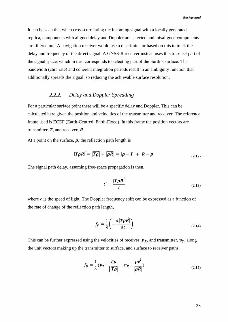
Background
33
It can be seen that when cross-correlating the incoming signal with a locally generated
replica, components with aligned delay and Doppler are selected and misaligned components
are filtered out. A navigation receiver would use a discriminator based on this to track the
delay and frequency of the direct signal. A GNSS-R receiver instead uses this to select part of
the signal space, which in turn corresponds to selecting part of the Earth’s surface. The
bandwidth (chip rate) and coherent integration periods result in an ambiguity function that
additionally spreads the signal, so reducing the achievable surface resolution.
2.2.2. Delay and Doppler Spreading
For a particular surface point there will be a specific delay and Doppler. This can be
calculated here given the position and velocities of the transmitter and receiver. The reference
frame used is ECEF (Earth-Centred, Earth-Fixed). In this frame the position vectors are
transmitter, 𝑻, and receiver, 𝑹.
At a point on the surface, 𝝆, the reflection path length is
|𝑻𝝆𝑹|⃗⃗ ⃗⃗ ⃗⃗ ⃗⃗ ⃗⃗ ⃗⃗ = |𝑻𝝆⃗⃗⃗⃗ ⃗| + |𝝆𝑹⃗⃗ ⃗⃗ ⃗| = |𝝆 − 𝑻| + |𝑹 − 𝝆| (2.12)
The signal path delay, assuming free-space propagation is then,
𝑡′ =
|𝑻𝝆𝑹|⃗⃗ ⃗⃗ ⃗⃗ ⃗⃗ ⃗⃗ ⃗⃗
𝑐 (2.13)
where 𝑐 is the speed of light. The Doppler frequency shift can be expressed as a function of
the rate of change of the reflection path length,
𝑓𝐷 =
1
𝜆(−
𝑑|𝑻𝝆𝑹⃗⃗⃗⃗⃗⃗⃗⃗ ⃗|
𝑑𝑡)
(2.14)
This can be further expressed using the velocities of receiver ,𝒗𝑹, and transmitter, 𝒗𝑻, along
the unit vectors making up the transmitter to surface, and surface to receiver paths.
𝑓𝐷 =
1
𝜆(𝒗𝑻 ∙
𝑻𝝆⃗⃗⃗⃗ ⃗
| 𝑻𝝆⃗⃗⃗⃗ ⃗|− 𝒗𝑹 ⋅
𝝆𝑹⃗⃗ ⃗⃗ ⃗
|𝝆𝑹⃗⃗ ⃗⃗ ⃗|)
(2.15)

34
For the calculation of the Doppler shift the surface is assumed to be stationary in this
reference frame, although surface currents and wave motion will additionally add small
perturbations to the signal through the movement of 𝝆.
2.2.3. Scattering Models
The parameter in the bistatic radar equation (2.1) that relates to the surface properties is the
scattering cross-section, 𝜎0. Determining the scattering cross-section then relating this to the
surface forms the basis of the GNSS-R sensing problem. GNSS-R has been proposed for
sensing of ice, land and ocean surfaces. The focus of this thesis is on the measurement of the
ocean surface roughness for which appropriate models are now introduced.
The scattering cross-section term can be further defined from the standard formulation in the
literature, as derived by [Barrick 1968]. The model is based on the Geometric Optics (GO)
limit to the Kirchhoff Approximation (KA) which is applicable to scattering in the quasi-
specular regime. This is when the radio wavelength is much smaller than the radius of
curvature of the surface, which is further defined in [Bass & Fuks 1977; Beckmann &
Spizzichino 1987].
The approach is based on splitting the surface into individual facets and summing the
contributions from facets that are aligned for specular reflection from receiver to transmitter.
This type of rough surface scattering is commonly referred to as quasi-specular scattering
because the scattering cross-section is directly proportional to the number of specularly
aligned facets on the surface [Brown, 1990]. A good reference for the general theoretical
basis for rough surface scattering is found in [Beckmann & Spizzichino 1987].
The summing of independent scattering elements in this model makes the assumption that the
surface is rough. The criterion for a statistically rough surface is normally expressed by the
Rayleigh criterion [Beckmann & Spizzichino 1987]. This specifies that the surface is rough if
the standard deviation of surface heights Δℎ is large compared to the radio wavelength 𝜆. A
surface is considered smooth under the condition,
Δℎ <
𝜆
8 cos(𝑖)
(2.16)
where 𝑖 is the incidence angle of the ray, (additionally defining the grazing angle as the
complement of the incidence angle, so that, 휀 = 𝜋/2 − 𝑖). Other scaling values are in use as

Background
35
there is a continuum between ‘smooth’ and ‘rough’ surfaces. The criterion from Equation
(2.16) is shown in Figure 2.7 against reflection elevation angle from the receiver for the GPS
L1 signal of wavelength 0.19 cm. The satellite altitude is 700 km and nadir is −90𝑜
elevation. For all reflections except near the Earth limb, the surface height variation would
need to be less than 5 cm for the scattering to be considered that of a smooth surface, which
means that the rough surface model provides a good fit for all ocean conditions. It will be
assumed that specular reflections will be chosen to avoid those near the horizon, otherwise
different scattering models will apply.
Figure 2.7 Rayleigh criterion between rough and smooth scattering, dependent on elevation angle from
satellite at 700km altitude
A review of modelling techniques for GNSS remote sensing of the ocean is provided in
[Ruffini, Cardellach, et al. 1999]. For ocean remote sensing with GNSS, the wavelengths are
long (19 cm at L1) compared to the wind induced ripples on the surface of the waves. The
Physical Optics (PO) or Kirchhoff Approximation (KA) improve on GO models by
modelling the electromagnetic fields with the surface facets being explicit re-radiating
antennas; which also assume that the radio wavelength is smaller than the characteristic
dimensions of the surface. Various approaches have been used to improve on the GO model,
the Integral Equation Method [Zuffada, Fung, et al. 2001], the Two-Scale Model which
models small waves on large swell, the Small-Slope Approximation [Elfouhaily, Thompson,
et al. 2002], and the realisations of explicit sea surfaces [Bian 2007] and [Clarizia, Di
Bisceglie, et al. 2009].
The model used in this research is that developed in [Zavorotny & Voronovich 2000], which
will be referred to as the Z-V model. This is formulated to describe the surface as an array of
facets. Each facet has a slope described by a Gaussian PDF, this effectively reduces the
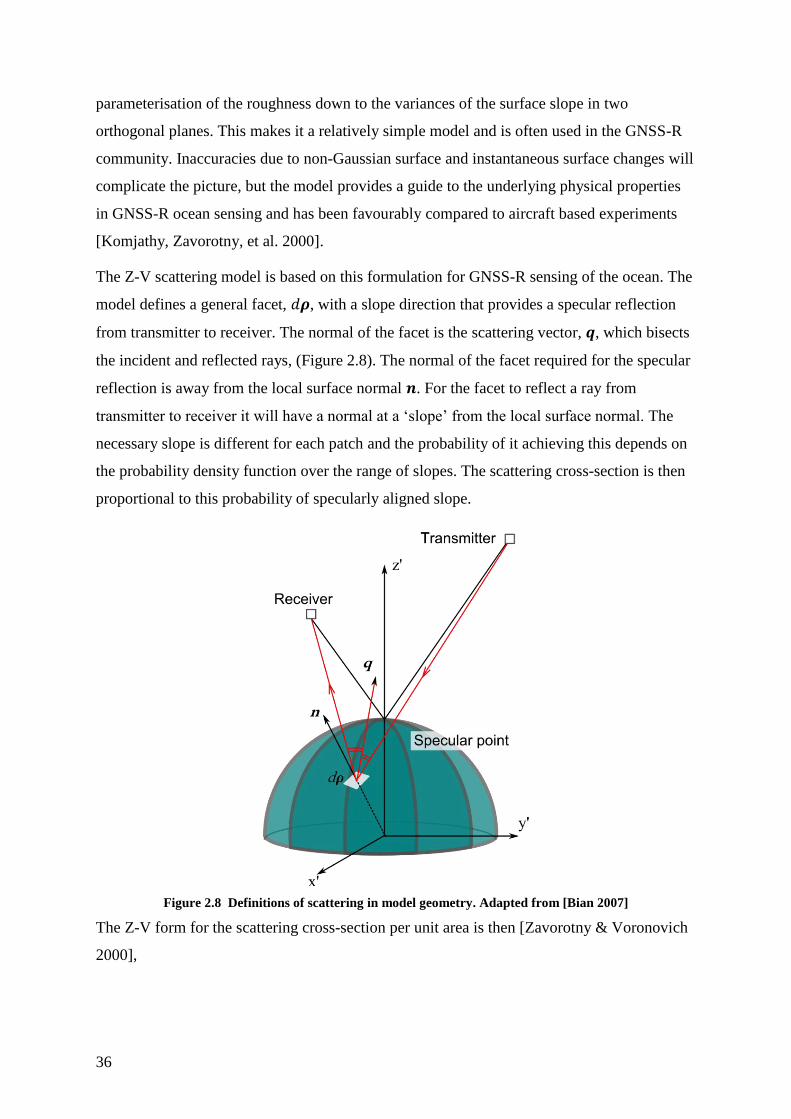
36
parameterisation of the roughness down to the variances of the surface slope in two
orthogonal planes. This makes it a relatively simple model and is often used in the GNSS-R
community. Inaccuracies due to non-Gaussian surface and instantaneous surface changes will
complicate the picture, but the model provides a guide to the underlying physical properties
in GNSS-R ocean sensing and has been favourably compared to aircraft based experiments
[Komjathy, Zavorotny, et al. 2000].
The Z-V scattering model is based on this formulation for GNSS-R sensing of the ocean. The
model defines a general facet, 𝑑𝝆, with a slope direction that provides a specular reflection
from transmitter to receiver. The normal of the facet is the scattering vector, 𝒒, which bisects
the incident and reflected rays, (Figure 2.8). The normal of the facet required for the specular
reflection is away from the local surface normal 𝒏. For the facet to reflect a ray from
transmitter to receiver it will have a normal at a ‘slope’ from the local surface normal. The
necessary slope is different for each patch and the probability of it achieving this depends on
the probability density function over the range of slopes. The scattering cross-section is then
proportional to this probability of specularly aligned slope.
Figure 2.8 Definitions of scattering in model geometry. Adapted from [Bian 2007]
The Z-V form for the scattering cross-section per unit area is then [Zavorotny & Voronovich
2000],
Background
37
𝜎0 = 𝜋|ℜ|2
𝒒4
𝑞𝑧4𝑃 (
−𝒒⊥
𝑞𝑧)
(2.17)
where,
ℜ = The polarisation dependant Fresnel reflection coefficient
𝒒 = The scattering unit vector: bisector of the incident and reflected rays
𝒒⊥ = The horizontal component of 𝒒 (Aligned to tangent of mean surface)
𝑞𝑧 = The vertical component of 𝒒. (Aligned to local surface normal)
𝑃 = The probability density function of the surface slopes
The polarization coefficient ℜ is calculated as a function of the dielectric properties of air and
seawater, wavelength and incidence angle. The surface ‘slope’ which has already been
referred to is now specifically defined as, 𝒒⊥/𝑞𝑧. The slope components are therefore the
horizontal components of the scattering vector divided by the vertical component, the result
of which is dimensionless.
Normally the most probable orientation of the surface facets is parallel to the mean sea
surface so 𝑃 is at is maximum when 𝒒⊥ = 𝟎. The scattering cross-section 𝜎0 has its
maximum at the specular direction of the mean surface, but extends out depending on 𝑃. This
forms the glistening zone around the specular point.
For the ocean surface, the effect of wind speed and direction are manifest in the distribution
of surface slopes, and hence in the slope PDF, P. The stronger the wind speed, the rougher
the surface and then the greater the variance in P. The direction along the maximal slope
variance indicates the wind direction. The scattering cross-section (2.17) does not specify a
particular PDF. It is helpful to link this back to the more general terminology, the slope PDF
is a specific measure of surface roughness.
For the Z-V model the slope PDF is a Gaussian function and the mean square slope (mss, by
convention) is the variance of the slopes. Alternatively, instead of parameterising the slope
PDF as Gaussian, it can be determined directly from a GNSS-R receiver from measurement
of 𝜎0 by substituting (2.17) into the radar Equation (2.1). There has been successful
application of this direct retrieval in aircraft trials [Cardellach & Rius 2007].
It is expected that the successful retrieval /of ocean roughness from GNSS-R will be from a
combination of empirical and theoretical inversion as ‘slope PDF’ does not provide a simple
38
correspondence to ocean conditions such as wind speed. By modelling the surface slopes in a
surface model parameterised by wind-speed it does provide us with an approach to predict the
sensitivity of GNSS-R to meteorological conditions. So a model of the ocean surface will
now be introduced to complete the simulation chain from surface to expected map of the
signal determined by the receiver.
2.2.4. Surface Model
The first relationship between the surface wind speed and the ocean surface slopes was
empirically determined from the analysis of photographs of sun glints by [Cox & Munk
1954]. Later work used scanning lasers, or pictures of sun glint from geostationary satellites
to improve the measurements. In parallel attempts have been made to theoretically reproduce
the experimental wave slope PDFs. A comparison of some of these models with experimental
data has been examined in [Anderson, Macklin, et al. 2000]. All of these have been
conducted at short, visual wavelengths and therefore do not necessarily represent completely
the scattering processes for the longer wavelength GNSS signals.
The model presented here is from [Elfouhaily, Chapron, et al. 1997] and is a commonly used
representation for GNSS bistatic sensing of the ocean, in the original Z-V model [Zavorotny
& Voronovich 2000] and other variations [Zuffada, Elfouhaily, et al. 2003]. This model is
used in Section 4.6 to analyse a new approach of retrieving ocean roughness from GNSS-R.
The Elfouhaily model describes the slope PDF of the ocean gravity-waves as a Gaussian
distribution. The variance in up-wind and cross-wind directions depends on the important
factors in wave generation: wind speed, the fetch and the time duration of that wind speed.
The model is given here for reference but the reader is advised to consult the original work
[Elfouhaily, Chapron, et al. 1997] or [Soulat 2003] for a full explanation. The formulation
here is that provided in [Gleason & Gebre-Egziabher 2009] which has an open-source
software implementation that has been used in this research. The model is developed using a
Cartesian coordinate system centred on the specular point: the x-axis is chosen to lie along
the intersection of the surface and the incidence plane (the plane containing the transmitter,
receiver and specular point 𝝆) and the z axis is the surface normal.
The surface slope of a facet on the surface is defined as 𝒔 = 𝒒⊥/𝑞𝑧, or decomposed into the
surface plane axes (𝑠𝑥, 𝑠𝑦) = (𝑞𝑥/𝑞𝑧, 𝑞𝑦/𝑞𝑧).
The bivariate Gaussian distribution of the slope 𝒔 is
Background
39
𝑃(𝑠𝑥, 𝑠𝑦) =
1
2𝜋√det(𝑀)exp [−
1
2(𝑠𝑥
𝑠𝑦)𝑇
𝑀−1 (𝑠𝑥
𝑠𝑦)]
(2.18)
where the matrix 𝑀 is
𝑀 = (
cos𝜑0 −sin𝜑0
sin 𝜑0 cos𝜑0) ⋅ (
𝜎𝑢2 0
0 𝜎𝑐2) ⋅ (
cos𝜑0 sin𝜑0
−sin𝜑0 cos𝜑0)
(2.19)
The angle 𝜑0 is the angle between the wind direction and the x-axis. The Gaussian shape of
the PDF being parameterised by the mean-square slope (mss) in the up-wind direction, 𝜎𝑢2,
and the cross-wind direction, 𝜎𝑐2. The matrix 𝑀 provides a rotation of the slope PDF into the
scattering coordinate frame, so is called the directional mean-square slope. The total mss is
𝜎𝑠2 = 2𝜎𝑢𝜎𝑐.
The slopes variance of the Gaussian PDF can be determined from the ocean surface elevation
wave-vector spectrum Ψ(𝜅, φ), which is integrated over (surface) wave numbers, 𝜅, and
azimuth angle 𝜑,
𝜎𝑢2 = ∫ ∫ 𝜅2 cos2 𝜑 Ψ(𝜅, φ)𝑑𝜅𝑑𝜑
𝜋
−𝜋
𝜅∗
0
𝜎𝑐2 = ∫ ∫ 𝜅2 sin2 𝜑 Ψ(𝜅, φ)𝑑𝜅𝑑𝜑
𝜋
−𝜋
𝜅∗
0
(2.20)
The KA considers the strong specular-like reflections and not the small-scale features that
would result in diffuse scattering. This means that a wavenumber cut-off is chosen to identify
features that constitute sufficiently large-scale roughness. There have been a number of cut-
off limits proposed in the literature, such as [Thompson, Elfouhaily, et al. 2005]. In this work
the wave number cut-off, 𝜅∗ used to divide the two scales will be that proposed by [Garrison,
Komjathy, et al. 2002], which is 𝜅∗ =2𝜋 cos(𝑖)
3𝜆 (where 𝑖 is the reflection incidence angle).
The variances of the slopes are determined mostly by the low-frequency region of the
spectrum (expressed by the integration limit 𝜅 ≤ 𝜅∗), from which it follows that the radar
cross-section is governed by slope variances associated with relatively long waves (0.5–1 m
scale or longer for L-band signals).
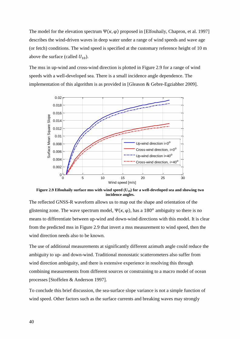
40
The model for the elevation spectrum Ψ(𝜅, φ) proposed in [Elfouhaily, Chapron, et al. 1997]
describes the wind-driven waves in deep water under a range of wind speeds and wave age
(or fetch) conditions. The wind speed is specified at the customary reference height of 10 m
above the surface (called 𝑈10).
The mss in up-wind and cross-wind direction is plotted in Figure 2.9 for a range of wind
speeds with a well-developed sea. There is a small incidence angle dependence. The
implementation of this algorithm is as provided in [Gleason & Gebre-Egziabher 2009].
Figure 2.9 Elfouhaily surface mss with wind speed (U10) for a well-developed sea and showing two
incidence angles.
The reflected GNSS-R waveform allows us to map out the shape and orientation of the
glistening zone. The wave spectrum model, Ψ(𝜅, φ), has a 180𝑜 ambiguity so there is no
means to differentiate between up-wind and down-wind directions with this model. It is clear
from the predicted mss in Figure 2.9 that invert a mss measurement to wind speed, then the
wind direction needs also to be known.
The use of additional measurements at significantly different azimuth angle could reduce the
ambiguity to up- and down-wind. Traditional monostatic scatterometers also suffer from
wind direction ambiguity, and there is extensive experience in resolving this through
combining measurements from different sources or constraining to a macro model of ocean
processes [Stoffelen & Anderson 1997].
To conclude this brief discussion, the sea-surface slope variance is not a simple function of
wind speed. Other factors such as the surface currents and breaking waves may strongly
0 5 10 15 20 25 300
0.002
0.004
0.006
0.008
0.01
0.012
0.014
0.016
0.018
0.02
Wind speed [m/s]
Surf
ace M
ean S
quare
Slo
pe
Up-wind direction i=0o
Cross-wind direction, i=0o
Up-wind direction i=40o
Cross-wind direction, i=40o

Background
41
impact the roughness as well. The wave spectrum models provide a link between wind speed
and the surface roughness that can be used to model a reflected GNSS signal and understand
the sensitivity of the GNSS reflection to the surface.
The following discussion introduces the fundamental GNSS-R receiver techniques for
mapping out the scattering cross-section.
2.3. GNSS-R Receiver
A typical GNSS navigation receiver tracks the PRN code signals through a combination of
delay locked loop for the code tracking and a frequency or phase locked loop for the carrier
Doppler tracking. In contrast a GNSS-R receiver determines surface properties through
mapping the signal delay cross-correlations and Doppler spread around that of the specular
point’s ray. The shape of the spreading can be related to the scattering zone on the surface
which in turn can be used to infer the surface roughness. The following section introduces the
conventional representation of the DDM as a map of the scattered power over delay and
Doppler.
A heterodyne radio receiver architecture is shown in Figure 2.10 which is a practical method
to digitise and subsequently process a radio frequency signal. The antenna is followed by
Low Noise Amplifier (LNA) and band-pass filter, to amplify and select the GNSS band. This
is followed by down conversion from the RF carrier frequency down to an Intermediate
Frequency (IF) by mixing with an oscillator. The IF signal is then further filtered by the anti-
aliasing filter before digital sampling with the Analogue to Digital Converter (ADC).
Figure 2.10 Schematic of down-conversion and sampling architecture used to produce an IF signal
The delay Doppler map is calculated from the IF output using Equation (2.6). The DDM is
formed from an array of these cross-correlations over a range of relative time delay, 𝑡′, and

42
carrier frequency, 𝑓′. Where the primed (′) notation specifies that the variable is locally
generated within the receiver as opposed to a particular quantity of the incoming signal.
Figure 2.11 Delay Doppler Map calculation array, showing recovery of the DDM.
The resulting calculation mapping is shown in Figure 2.11, for a 3 Doppler pixels by 7 delay
pixels realisation. The rows of the DDM have a constant delay offset, Δ𝑡, from each other.
Similarly the columns of the DDM correspond each to a different fixed Doppler frequency
spaced by Δ𝑓.
The DDM is conventionally plotted with the delay and Doppler axes as in Figure 2.12 and the
correlation power indicated by mapping to a colour.

Background
43
Figure 2.12 Delay Doppler map, grid of delay and Doppler. Each pixel’s value represents the correlation
power for that delay and Doppler
A GPS signal is received by multiplying the incoming signal, 𝑢(𝑡), by a replica code and
carrier frequency. For the signal to be received out of the noise the replica code and carrier
must align with that in 𝑢(𝑡).
Revisiting the cross-correlation calculation from Equation (2.6), but explicitly defining the
incoming PRN code chip rate, 𝑓𝑐, as well as the carrier frequency, 𝑓𝐿. Additionally the
propagation delay 𝜏 is set to zero to aid clarity, so that integration becomes,
𝑤(𝑡′, 𝑓′) =
𝐴 𝑑
𝑇𝑐𝑜ℎ∫ 𝑐(𝑓𝑐, 𝑡) 𝑐(𝑓𝑐
′, 𝑡 − 𝑡′) exp( 𝑗2𝜋(𝑓𝐿 − 𝑓𝐿′)𝑡 + 𝜙)
𝑇𝑐𝑜ℎ
0
𝑑𝑡 + 𝑛𝑤 (2.21)
The replica code 𝑐(𝑓𝑐′, 𝑡 + 𝑡′) has a chip frequency, 𝑓𝑐
′, time delay, 𝑡′, and the local carrier is
generated with frequency 𝑓′𝐿.
The code rate is a fixed division of the carrier frequency, so that 𝑓𝐿 = 𝑁 ⋅ 𝑓𝑐. For example the
GPS L1 carrier is exactly 1540 times higher than the C/A code modulation rate, so 𝑁 =
1540. The frequency of the transmitted carrier and the code are linked by this fixed ratio and
therefore the code rate would vary with the Doppler frequency across the DDM. In a DDM
accumulated over a time period a shift in code delay would occur for each column of the
DDM, due to the code rate changing with the Doppler frequency. A long integration would
result in a drift in code phase across the DDM by the end of the integration time.
Taking the Doppler axis: the Doppler effect causes a deviation in carrier frequency of the
received signals. The non-relativistic Doppler equation is
Δ𝑓𝐿 =
−𝑣 𝑓𝐿𝑐
(2.22)
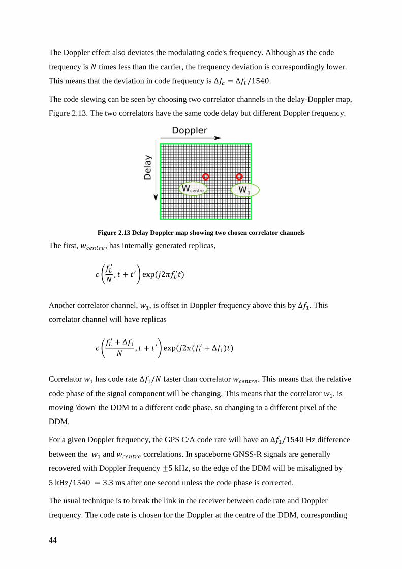
44
The Doppler effect also deviates the modulating code's frequency. Although as the code
frequency is 𝑁 times less than the carrier, the frequency deviation is correspondingly lower.
This means that the deviation in code frequency is Δ𝑓𝑐 = Δ𝑓𝐿/1540.
The code slewing can be seen by choosing two correlator channels in the delay-Doppler map,
Figure 2.13. The two correlators have the same code delay but different Doppler frequency.
Figure 2.13 Delay Doppler map showing two chosen correlator channels
The first, 𝑤𝑐𝑒𝑛𝑡𝑟𝑒, has internally generated replicas,
𝑐 (
𝑓𝐿′
𝑁, 𝑡 + 𝑡′) exp (𝑗2𝜋𝑓𝐿
′𝑡)
Another correlator channel, 𝑤1, is offset in Doppler frequency above this by Δ𝑓1. This
correlator channel will have replicas
𝑐 (
𝑓𝐿′ + Δ𝑓1
𝑁, 𝑡 + 𝑡′) exp (𝑗2𝜋(𝑓𝐿
′ + Δ𝑓1)𝑡)
Correlator 𝑤1 has code rate Δ𝑓1/𝑁 faster than correlator 𝑤𝑐𝑒𝑛𝑡𝑟𝑒. This means that the relative
code phase of the signal component will be changing. This means that the correlator 𝑤1, is
moving 'down' the DDM to a different code phase, so changing to a different pixel of the
DDM.
For a given Doppler frequency, the GPS C/A code rate will have an Δ𝑓1/1540 Hz difference
between the 𝑤1 and 𝑤𝑐𝑒𝑛𝑡𝑟𝑒 correlations. In spaceborne GNSS-R signals are generally
recovered with Doppler frequency ±5 kHz, so the edge of the DDM will be misaligned by
5 kHz/1540 = 3.3 ms after one second unless the code phase is corrected.
The usual technique is to break the link in the receiver between code rate and Doppler
frequency. The code rate is chosen for the Doppler at the centre of the DDM, corresponding

Background
45
to the specular path ray (for 𝑤𝑐𝑒𝑛𝑡𝑟𝑒) then the code rate is fixed for all columns of the DDM.
This does not materially affect the recovery of the signal as the usual coherent integration
time is of the order of milliseconds (as shown in section 2.3.2), so the chip error of 3.2 ⋅ 10−3
chips per millisecond, which will be a fraction of the digitised sample period.
From measurement of the DDM, the reflectivity of the scattering zone can be determined,
however the mapping from delay and Doppler to the surface are complicated by the sensing
geometry around the specular point.
2.3.1. Mapping the DDM to the Surface
The stages of the measurement concept are illustrated in Figure 2.14. The scattering of the
GNSS signal is spread out from the specular point over the scattering zone by the distribution
of the surface slopes (Figure 2.14, Left). Each point on the surface has a corresponding delay
from the specular path marked as rings of the same path length, iso-delay and a
corresponding Doppler frequency marked as curves of equivalent range-rate or iso-Doppler
(Figure 2.14, Centre)
Figure 2.14 Mapping from surface scattering locations to the signal space in the delay-Doppler map
From the GNSS-R receiver it is possible only to take measurements of the reflected signal,
not directly the surface slopes. The receiver can only measure the reflection through mapping
out the reflected power in signal-space. The surface scattering zones from (Figure 2.14,
Centre) are shown with their correspondence to the signal zones in (Figure 2.14, Right).
Positions on the surface (A) to (F) , can be matched up to their corresponding points in the
DDM:

46
(A) → The specular point.
(B), (C) → Positions on the surface ‘in front’ and behind the specular point in
relation to the receiver’s motion.
(D), (E) → Positions either side of the specular point, (in and out of page in Figure
2.14, Left).
(F) → Above the surface.
It is noted that there is an ambiguity, such that spatially separated points (D) and (E)
correspond to the same signal properties. The ambiguous nature of the mapping from spatial
coordinates to DDM coordinates complicates the inversion of the DDM back to the surface
slope distribution.
2.3.2. DDM Sensitivity to Ocean Roughness
There are a number of previous studies into the sensitivity of GNSS-R measurements to sea
state and the surface roughness such as [Bian 2007], [Fung, Zuffada, et al. 2001], [D’Addio
& Buck 2008] and [Elfouhaily, Thompson, et al. 2002]. These generally agree on the DDM
having a good sensitivity to the roughness for wind speeds under about 10 m/s, however a
relatively poor sensitivity to wind direction.
Here the sensitivity analysis will not be repeated, but two example DDMs are modelled using
the roughest and smoothest ocean conditions to give a qualitative analysis of DDM sensitivity
to the waves. The scattering model as set out in this chapter combines the bistatic radar
equation, the Z-V scattering model, and the Elfouhaily surface model. For this work
particular contribution is provided from the work of [Gleason & Gebre-Egziabher 2009] and
[Clarizia, Gommenginger, et al. 2008]. From this model the two extreme case DDMs are
formed for the low-Earth orbit satellite receiver geometry. The chosen receiver, and
transmitter geometry is a receiver at 690 km altitude and the reflection away from the
receiver nadir by 14.8𝑜.
The slope variances for the smoothest and roughest ocean conditions have been taken from
the Elfouhaily surface model shown in Figure 2.9. The up-wind and cross-wind surface slope
variances were chosen to be equal, to exclude wave direction dependence. For smooth
surface DDM in Figure 2.15(A), mss = [0.001, 0.001] and for the roughest surface DDM
in Figure 2.15(B), mss = [0.016, 0.016].
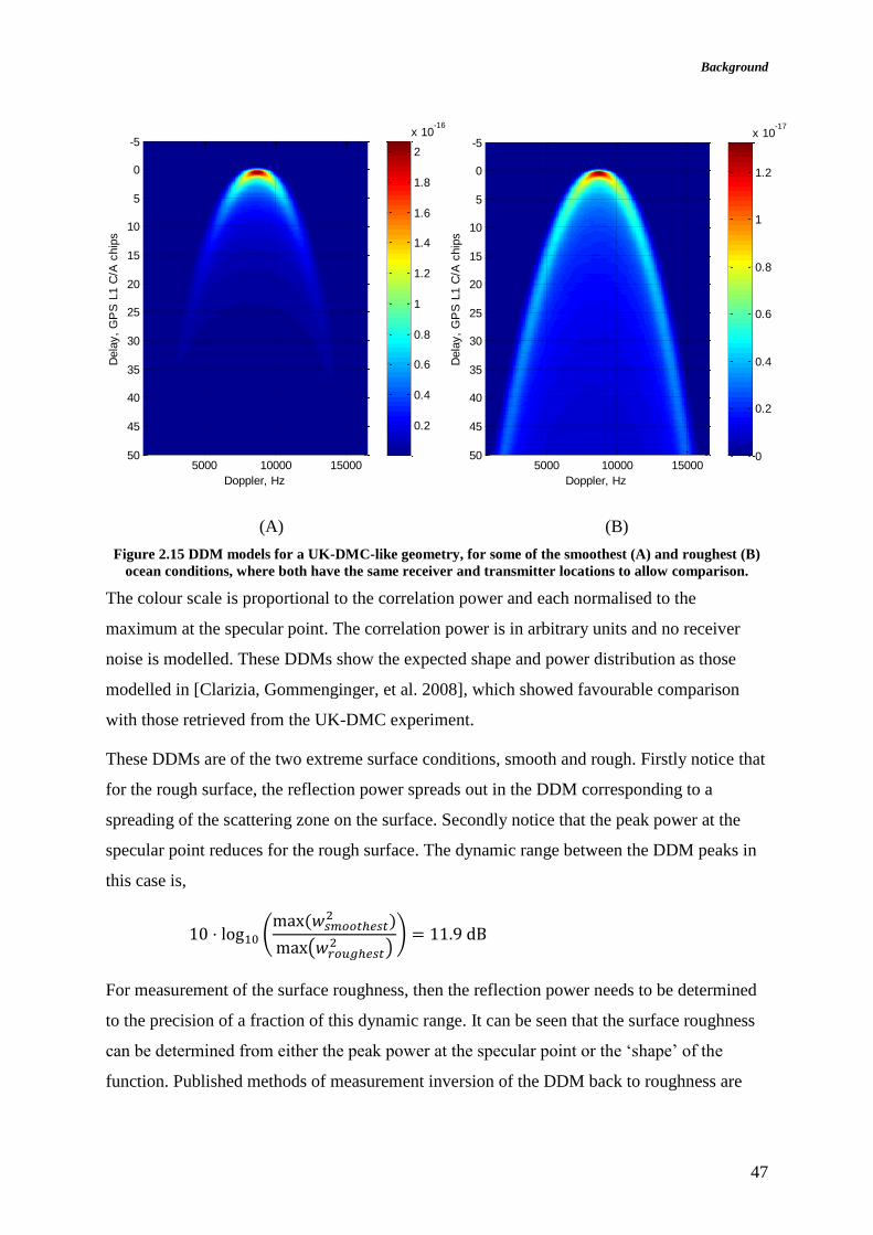
Background
47
(A) (B)
Figure 2.15 DDM models for a UK-DMC-like geometry, for some of the smoothest (A) and roughest (B)
ocean conditions, where both have the same receiver and transmitter locations to allow comparison.
The colour scale is proportional to the correlation power and each normalised to the
maximum at the specular point. The correlation power is in arbitrary units and no receiver
noise is modelled. These DDMs show the expected shape and power distribution as those
modelled in [Clarizia, Gommenginger, et al. 2008], which showed favourable comparison
with those retrieved from the UK-DMC experiment.
These DDMs are of the two extreme surface conditions, smooth and rough. Firstly notice that
for the rough surface, the reflection power spreads out in the DDM corresponding to a
spreading of the scattering zone on the surface. Secondly notice that the peak power at the
specular point reduces for the rough surface. The dynamic range between the DDM peaks in
this case is,
10 ⋅ log10 (max (𝑤𝑠𝑚𝑜𝑜𝑡ℎ𝑒𝑠𝑡
2 )
max(𝑤𝑟𝑜𝑢𝑔ℎ𝑒𝑠𝑡2 )
) = 11.9 dB
For measurement of the surface roughness, then the reflection power needs to be determined
to the precision of a fraction of this dynamic range. It can be seen that the surface roughness
can be determined from either the peak power at the specular point or the ‘shape’ of the
function. Published methods of measurement inversion of the DDM back to roughness are
Dela
y,
GP
S L
1 C
/A c
hip
s
Doppler, Hz
5000 10000 15000
-5
0
5
10
15
20
25
30
35
40
45
50
0.2
0.4
0.6
0.8
1
1.2
1.4
1.6
1.8
2
x 10-16
Dela
y,
GP
S L
1 C
/A c
hip
s
Doppler, Hz
5000 10000 15000
-5
0
5
10
15
20
25
30
35
40
45
50 0
0.2
0.4
0.6
0.8
1
1.2
x 10-17

48
discussed in Section 2.3.5, but first two of the practical receiver challenges in forming the
DDM measurement are discussed.
2.3.3. Coherence Time
When processing the DDM in the GNSS-R receiver, the aim is to extract the maximal signal
power to reduce the variance of the 𝜎0 estimate and hence provide the best estimate of the
surface roughness. To improve the DDM power estimate the coherent integration time needs
to be optimised.
There are two constraints to the length of the receiver’s coherent integration time, 𝑇𝑐𝑜ℎ. Both
constraints occur when the phase of the signal starts to destructively interfere with itself due
to a change in the phase of signal component during the integration time. The first cause is a
movement in the scattering surface. A half-wavelength change in path length would cause
destructive interference. For a nadir reflection, this corresponds to a quarter-wavelength
vertical displacement, which is (0.25 ⋅ 0.19) m for GPS L1. Approximating the surface
waves to the linear (Airy) wave theory in deep water [Holthuijsen 2007] then the vertical
displacement, ℎ, is
ℎ(𝑥, 𝑡) = 𝐴 cos(𝑘𝑥 − 𝜔𝑡) (2.23)
Where 𝐴 is the surface wave amplitude, 𝑘 the angular wave number in radians per metre and
the angular frequency 𝜔 = 2𝜋𝑓 for deep water.
Differentiating (2.23), then the rate of change of vertical displacement is
𝑑ℎ(𝑥, 𝑡)
𝑑𝑡= 𝜔𝐴 sin(𝑘𝑥 − 𝜔𝑡)
(2.24)
which has maximum velocity of 𝜔𝐴. The time taken to move by quarter of the RF
wavelength sets the maximum coherence time, so that
𝑡𝑐𝑜ℎ <
𝜆
4𝜔𝐴
(2.25)
Where 𝜆 is the RF wavelength (as opposed to the surface wave length). From the Pierson-
Moskowitz wave spectrum [Pierson & Moskowitz 1964] a well-developed sea for a 25 m/s
wind speed results in a wave spectrum with peak at wave period 20 seconds and Significant

Background
49
Wave Height (SWH) 15 m. For this rough analysis the SWH can be equated to wave
amplitude, making the coherence time limit 𝑡𝑐𝑜ℎ < 10 ms.
The second limit on coherence time is due to the movement of the receiver over the surface.
For a particular pixel of the delay Doppler map, the surface is selected through the bistatic
radar equation to lie along the chosen iso-Doppler line. This amounts to spatial filtering
described in (2.10) by the sinc term,
𝜒(𝑓 − 𝑓′) = sinc(𝜋(𝑓 + 𝑓𝐷 − 𝑓′)𝑇𝑐𝑜ℎ) (2.26)
From this it can be seen that fixing the integration time is the equivalent of setting the
bandwidth of the receiver and setting the spatial footprint. There is a match in frequency
along the iso-Doppler line, but further from this line, oscillations outside of this bandwidth
are attenuated. The coherent integration time should therefore be set such that the bandwidth
is sufficient for the largest surface zone. The 1st iso-range ellipse which is the surface
corresponding to specular point delay to an additional delay of one code chip, 𝑇𝑐, sets the
limit for the integration time as it is the largest spatial zone selected by the iso-range lines.
(A) (B)
Figure 2.16 Illustration of the lines of iso-delay and iso-Doppler on the surface, defining the size of the 1st-
iso-range ellipse. (A) Perspective view (B) Plan view of surface.
The mean sea surface provides a relatively difficult surface to determine the analytical
functions for understanding the GNSS-R iso-delay and iso-Doppler lines. The geometry can
be simplified using the first-order approach of [Hajj, Zuffada, et al. 2002]. A planar surface is
constructed tangential to the Earth’s surface. This approximation is appropriate for the size of

50
the 1st iso-delay ellipse as the spherical Earth does not have a large departure from the plane
over this distance.
The iso-delay ellipses are found from the intersection of the plane with an ellipsoid having
foci at the transmitter and receiver locations. Without deriving this, but taking the result from
Hajj and Zuffada, the dimensions of the 1st iso-range ellipse are found from the intersection
of the ellipsoid and surface plane. The ellipse on the surface has semi-minor and semi-major
axes,
𝑎 =1
sin 휀(|𝑹𝑺⃗⃗⃗⃗ | |𝑻𝑺⃗⃗⃗⃗ | 𝑇𝑐 𝑐
|𝑹𝑺⃗⃗⃗⃗ | + |𝑻𝑺⃗⃗⃗⃗ |)
12
, 𝑏 = (|𝑹𝑺⃗⃗⃗⃗ | |𝑻𝑺⃗⃗⃗⃗ | 𝑇𝑐 𝑐
|𝑹𝑺⃗⃗⃗⃗ | + |𝑻𝑺⃗⃗⃗⃗ |)
12
(2.27)
where 𝑇𝑐 is the code chip rate, 𝑐 the speed of light and the distances |𝑹𝑺⃗⃗⃗⃗ ⃗|, |𝑻𝑺⃗⃗⃗⃗ ⃗|, as defined in
Figure 2.16.
Taking the same approach as in [Lowe, LaBrecque, et al. 2002a], the field from the specular
point can be approximated to that generated from a uniformly illuminated circular aperture,
with the size corresponding to the 1st iso-range ellipse. A uniformly illuminated aperture has
a first null at 1.22 ⋅ 𝜆/𝐷 rad, where D is the diameter of the aperture. For a receiver moving
through this field with speed 𝑣𝑅, at distance |𝑹𝑺⃗⃗⃗⃗ ⃗| from the specular point, the signal will go
from peak to null in time 𝑇𝑐𝑜ℎ.
𝑇𝑐𝑜ℎ =
1.22 ⋅ 𝜆 ⋅ |𝑹𝑺⃗⃗⃗⃗ |
𝐷 ⋅ 𝑣𝑅
(2.28)
For the geometry of a nadir reflection observed by a low-Earth orbit satellite of altitude
700 km, and orbital velocity 6.5 km/s, then diameter of the iso-range ellipse, D, is 14 km.
This leads to a maximum coherence time of 𝑇𝑐𝑜ℎ = 1.7 ms. This is considerably shorter than
that for an airborne GNSS-R receiver, for example 10 ms coherent integration was used in a
low altitude aircraft experiment, [Ruffini, Soulat, et al. 2004].
The short coherence time available in spaceborne GNSS-R leads to the need for further
averaging of the correlation through non-coherent averaging to bring the signal out of the
noise.

Background
51
2.3.4. Coherent and Non-Coherent Integration
The aim of the scatterometric measurement is to determine the surface roughness from its
reflectance, which means measurement of reflected signal power in relation to incident
power. The processing gain will depend on the length of the coherent integration and the
subsequent averaging.
The coherence time is limited to little more than 1 ms by the geometry of the scattering as
determined in the previous section, it is necessary to average the signal further in incoherent
accumulations (these are known as multiple looks in radar terminology). The coherent
integration 𝑤 from Equation (2.6) is a complex phasor, so the incoherent accumulation over
𝑀 results is the average of the power of these phasors:
�̂�(𝑡′, 𝑓′) =1
𝑀∑|𝑤(𝑡′, 𝑓′)|2𝑀
𝑛=1
(2.29)
where we use the accented notation to mean a measurement output of the receiver. The
summation index is 𝑛, of the total 𝑀 averaged looks, each over the coherent integration time,
𝑇𝑐𝑜ℎ.
Assuming that only white Gaussian noise is present on the I and Q channels of 𝑤, the
probability density function describing the noise power, |𝑤|2, follows a Rayleigh
distribution, then according to the central limit theorem for large 𝑀 the result �̂� yields a
Gaussian distribution.
The standard deviation of the result drops with the square root of the number of independent
looks 𝑀, if it can be assumed that each of the looks is statistically independent [Richards
2009], so that the absolute Signal to Noise Ratio (SNR) is,
Γ = √𝑀 ⋅
𝑇𝑐𝑜ℎ ⋅ �̂�
�̅�
(2.30)
where �̅�, is the mean noise power. Typically for space-borne GNSS-R the reflected signals
are very weak so the focus is on recovering the signal to retrieve the lowest variance in the
estimate of the signal power. The coherent integration time 𝑇𝑐𝑜ℎ would be chosen to be the
maximum for the receiver and transmitter geometry. One limit on the incoherent integration

52
is the rate of the specular point movement, as the specular point moves at around 6.5 km/s
(for a 700 km altitude receiver) a long integration will result in poor surface resolution.
As an example, the UK-DMC GNSS-R experiment would typically use a coherent integration
time, 𝑇𝑐𝑜ℎ, of 1 ms and these were then incoherently accumulated for 𝑀 = 1000 times to total
a 1 second integration. The total integration time will be labelled, 𝑇𝑖𝑛𝑐𝑜ℎ.
As GNSS-R has limits on the coherence time and the total integration time, it is helpful to
express the number of looks as
M =
𝑇𝑖𝑛𝑐𝑜ℎ
𝑇𝑐𝑜ℎ
(2.31)
so that the absolute signal to noise ratio will be,
Γ = 𝑇𝑐𝑜ℎ√𝑇𝑖𝑛𝑐𝑜ℎ
𝑇𝑐𝑜ℎ⋅�̂�
�̅�= √𝑇𝑐𝑜ℎ 𝑇𝑖𝑛𝑐𝑜ℎ ⋅
�̂�
�̅�
(2.32)
It is important to distinguish between the signal to noise ratio at the receiver input and that
determined following receiver processing. Two measures are used in this thesis for the signal
to noise ratio. The first is that of the absolute signal to noise ratio as defined in Equation
(2.32). The second is the processed signal to noise,
Γ0 =
�̂� − �̅�
RMS(�̂�)
(2.33)
where RMS(�̂�) is the Root Mean Squared of the measured noise. Processed signal to noise
ratio gives an indication of the detectability of the signal from the noise. This is a relevant
measurement as it provides a measure of the variance of the signal, which is important in
determining the ability to match the DDM to the scattering model for retrieving the surface
roughness.
2.3.5. Measurement Inversion
The theoretical models provide a tool to recover the sea surface slope from the measurements
of the scattered signal power provided by a GNSS-R sensor. In both studies, [Clarizia,
Gommenginger, et al. 2009] and [Ruffini, Soulat, et al. 2004] the scattered signal power is

Background
53
modelled over a two-dimensional delay-Doppler map and a least-squared fit of the modelled
DDM with the measured DDM is used to estimate the variance of the sea-surface slope. In
addition empirical approaches have been made by [Gleason & Adjrad 2005]
At the present time another PhD student, Maria Paola Clarizia, has been working on GNSS-R
at the National Oceanographic Centre (NOC), Southampton. Analysis of the UK-DMC delay
Doppler maps has been carried out for her masters project [Clarizia, Gommenginger, et al.
2008] and the work is continuing in a PhD focusing on development of a GNSS-R ocean
scattering model. This is distinct from the aims of this research which is focused more
towards the receiver design. There is a strong interdependence between the ocean models and
the receiver design and there is ongoing collaboration.
Most existing work on matching experimental GNSS-R to theoretical descriptions has
concentrated on airborne and ground-based receiving systems [Cardellach, Ruffini, et al.
2003], [Komjathy, Zavorotny, et al. 2000]. The interest in this project is for a spaceborne
system so measurements can reach into less accessible areas such as mid-ocean to provide a
global coverage. From the study of GNSS-R from low altitude receivers, some extrapolation
can be made to the operation of a spaceborne receiver. The spaceborne systems will operate
in a different parameter space however, due to the magnitude of the differences in speed and
distance from the surface. The different receiver geometry may result in sensitivities to
different surface phenomena. The constraints on the hardware design of a spaceborne
receiver are also significantly different from an airborne receiver.
With these differences in mind, the remainder of this chapter will provide a review of the
planned and existing GNSS-R receivers and experiments.
2.4. UK-DMC and On-Going Work at Surrey
With the aim of driving the development and commercial exploitation of GNSS-
Reflectometry from space, SSTL built an experimental GPS reflectometry receiver into its
UK-DMC satellite [Unwin, Gleason, et al. 2003]. In 2003 the UK-DMC satellite was
launched as part of the international disaster monitoring constellation. The satellite is at
nominal altitude about 680 km altitude in a sun-synchronous orbit, carrying a primary
payload of a multispectral optical imager.
The experimental receiver consists of a navigational receiver, with modifications to allow
recording of the raw signal for short periods of time. An 11.6 dBi fixed gain LHCP antenna

54
was accommodated on the nadir-pointing face of the satellite. The radio front-end chipsets
output 2 bit samples to a data logger. Data from both the nadir and zenith antennas are
recorded for 20 seconds. This is then sent down to the ground for post-processing, (Figure
2.17 and Figure 2.18).
Figure 2.17 Schematic of UK-DMC GNSS-R receiver hardware. Courtesy of SSTL.
Figure 2.18 Modifications to the SGR-20 GPS receiver to allow connection to the data-logger. Courtesy of
SSTL.
The experiment was more successful than anticipated given the low link margin in the RF
chain and reflected signals have been detected over the ocean, ice and even dry land.
Researchers at the University of Surrey have analysed the data archive and it has been the
basis of two PhDs. In [Gleason 2006] the data was collected, receiver processing developed
and amongst in-depth analysis of the signal statistics, a correlation was demonstrated between
sea-state and the measured signals. Following from this a refined ocean scattering model and

Background
55
an inversion method from the DDM to ocean-roughness measurement was developed in
[Bian 2007] and [Bian, Pechev, et al. 2006]. The UK-DMC data is still under-utilised with
the potential for further analysis with alternative techniques or the data analysed for other
applications.
The UK-DMC satellite has been used to support this PhD by collecting reflections from the
first Galileo signals and experimentally testing approaches for reflection processing and
tracking. As a result of this the data has been catalogued, which is reproduced in part in
Appendix E.
This mission demonstrated the potential for GPS reflectometry, to be incorporated as a
primary or secondary payload on a small remote sensing satellite. The instrument also
highlighted the benefits of a flexible receiver architecture that would allow processing in a
variety of ways to be tailored to different types of Earth surfaces. The UK-DMC experiment
has allowed a number of lessons to be learnt which can now be used to optimise the design of
the next generation receiver which SSTL is developing, called the SGR-ReSI.
2.4.1. SGR-ReSI and TechDemoSat-1
During the course of this project SSTL has, in parallel, been developing a new GNSS
receiver architecture called the SGR-ReSI (Space GNSS Receiver Remote Sensing
Instrument). It is designed to be multi-frequency, multi-constellation, with additional data
processing capabilities and on board data storage, Figure 2.19. The core of the SGR-ReSI is a
GNSS navigation receiver with 24-channels for GPS L1 and support for up to 4 antennas [De
Vos van Steenwijk, Unwin, et al. 2010]. The SSTL developed GNSS correlators are
implemented alongside a LEON3 soft-core processor in an Actel ProASIC3 FPGA. The
Actel ProASIC3 is a non-volatile Flash-based FPGA that consumes little power, providing a
low-power GNSS receiver for the basic orbit determination and timing functions typically
required of satellite platform GNSS receivers.
Alongside the navigation core is a reconfigurable co-processor that can be configured for
other processing techniques, this has been included with the notion of support for GNSS
radio occultation and GNSS reflectometry.

56
Figure 2.19 SGR-ReSI system diagram. Courtesy of SSTL
The architecture is designed for capturing the data needed for validating the surface
measurement accuracy of spaceborne GNSS-R. This is through both improving the data-
logger functionality equivalent to the experiment on UK-DMC and improving on the volume
of data captured through real-time reflectometry processing. It is the SGR-ReSI and in
particular the reprogrammable co-processor that will form the platform for the developments
in this PhD. This PhD contributes to the development of this receiver for the application of
GNSS-R and improves on the state of the art through real-time GNSS-R processing which is
detailed in Chapter 5.
The SGR-ReSI is currently being integrated into the UK TechDemoSat-1 (TDS-1) funded by
the UK government Technology Steering Board. A rendering of the satellite, including the
GNSS-R antenna is shown in Figure 2.20.
Figure 2.20 Rendering of TechDemoSat-1 in orbit. Courtesy of SSTL.

Background
57
2.5. Instruments in Development
A number of other organisations are developing GNSS-R instruments, which will now be
introduced.
2.5.1. ESA: PARIS
The European Space Agency (ESA) has been developing the principle of GNSS
reflectometry for a number of years as part of their Passive Reflectometry and Interferometry
System (PARIS) concept. It was first proposed in the ESA Journal in 1993 [Martin-Neira
1993] as a tool to study mesoscale ocean altimetry.
One significant difference in the PARIS concept to that used in most other GNSS-R concepts,
is that the reflected signals are correlated against the direct signals, to allow use of the non-
public GNSS signals. This means that a high gain antenna beam needs to be steered to each
of the GNSS transmitters to record the transmitted signal. The zenith pointing antenna would
be made the same size as the nadir antenna to receive a sufficiently strong direct signal and
separate out signals from individual GNSS transmitters. The antenna would consequentially
be considerably larger than that needed if the GPS codes were generated as replicas on-board
and synchronised with a standard GPS navigation receiver. One particular benefit is that the
all GNSS signals can be used, even the encrypted wideband GPS military P(Y) code and the
restricted access Galileo codes. These signals would not be available to a system using a low-
gain zenith antenna.
Astrium UK have built a PARIS airborne demonstrator (PAD) which underwent cliff-top and
airborne trials [Buck & D’Addio 2007]. An in-orbit demonstrator satellite is currently being
proposed [Martín-Neira, D’Addio, et al. 2011]. This would have a 1.1m antenna with up and
down looking elements. Antenna beams will be steered in analogue electronics to four
specular reflections and the associated four GNSS transmitters. The altimetry performance
error budget predicts a 1 standard deviation precision of 17cm. The mass budget for the
payload is 44kg and consuming 46W. The schedule is for a launch in about 5 years subject to
approval of funding [ESA 2008].
58
2.5.2. NASA / JPL
JPL were the first group to detect GPS reflections from space, using an existing data set from
the SAC-C imaging radar experiment carried on-board the U.S. Space Shuttle [Lowe,
LaBrecque, et al. 2002b].
JPL has also been developing its own GNSS reflectometry instrument as part of the NASA
instrument incubator program. The TOGA instrument (Time-shifted Orthometric GNSS-
Array) is designed to address GNSS reflectometry science needs in a flexible prototype
[Meehan, Esterhuizen, et al. 2007]. In some important aspects it is very similar to the PARIS
concept. The development is aimed at providing surface altimetry from Low Earth Orbit
(LEO).
An electronically steerable array antenna is used to target multiple reflections simultaneously
with a high-gain beam. For multiple beam-forming, the RF output of each antenna element is
down-converted and digitised. This is done in a purpose built ASIC called the RF Down
Converter Array (RFDC), Figure 2.21. This stage amplifies and separates the L1, L2 and
L5(E5) signals before digitisation. For each antenna and each frequency an RFDC chip is
needed, so in the prototype system, 48 chips will be tested. To give an idea of scale: the
architecture is designed to accommodate 192 RFDC chips for the full 64 element system.
After digitisation, the following stage is the Reconfigurable Digital Processor (RDP) which
applies the phasing between signals for the beam-forming. This is implemented in digital
logic in Field Programmable Gate Arrays (FPGAs). The GNSS Real-time Receiver (GRR)
then processes the reflected signals. All of these functions are controlled by the Science
Processor (SP) implemented in a Linux based computer.
The prototype version uses a 2m wide antenna array, and consumes around 100 W of power.
The TOGA design approach is focused on achieving altimetry and most of the hardware is in
the large beam-steered antenna. The receiver design has since been transformed into the TriG
receiver, which focuses on Radio Occultation, [Esterhuizen, Franklin, et al. 2009].

Background
59
Antenna:
16-64 antenna elements
2 x 8 elements in prototype
20 dB peak gain at L1 frequency
200 x 50 x 10cm
Figure 2.21 Schematic of TOGA instrument. NASA [Meehan, Esterhuizen, et al. 2007]
2.5.3. UPC, Barcelona
The Passive Advanced Unit (PAU) under development at the Universitat Politecnica de
Catalunya , Barcelona is a suite of instruments that includes an L-band radiometer, an infra-
red radiometer and a GNSS reflectometer. An overview of the instrument concept is given in
[Camps, Bosch-Lluis, et al. 2007]. The PAU instrument shares the same radio hardware
between the L-band radiometer and the GNSS-R instrument.
The GNSS-R component of the system has been developed into a prototype receiver for
airborne trials. This has been developed in two streams. The PAU-OR (Passive advanced unit
one receiver) is a real-time processing receiver with a dual-polarisation 7 patch array antenna
giving a 17.5 dBi gain. The details of the GPS reflectometry part are presented in [Marchan-
Hernandez, Ramos-Perez, et al. 2007] and [Valencia, Camps, et al. 2010].
2.5.4. IEEC
IEEC have built the GOLD-RTR instrument as an airborne demonstrator of GNSS-R.
GOLD-RTR stands for: GPS open-loop differential real-time receiver. The Gold-RTR
instrument is based on commercial parts and FPGAs mounted into a 19 in rack (Figure 2.22).
Only the GPS C/A code is received. The GOLD-RTR receiver processes the signal in real-
time, generating the cross-correlated waveform automatically [Nogues-Correig, Cardellach
Gali, et al. 2007]. The waveform is then parametrised and recorded.
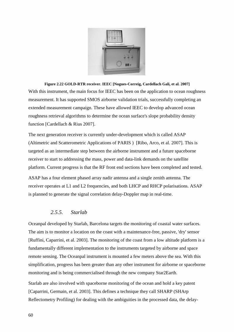
60
Figure 2.22 GOLD-RTR receiver. IEEC [Nogues-Correig, Cardellach Gali, et al. 2007]
With this instrument, the main focus for IEEC has been on the application to ocean roughness
measurement. It has supported SMOS airborne validation trials, successfully completing an
extended measurement campaign. These have allowed IEEC to develop advanced ocean
roughness retrieval algorithms to determine the ocean surface's slope probability density
function [Cardellach & Rius 2007].
The next generation receiver is currently under-development which is called ASAP
(Altimetric and Scatterometric Applications of PARIS ) [Ribo, Arco, et al. 2007]. This is
targeted as an intermediate step between the airborne instrument and a future spaceborne
receiver to start to addressing the mass, power and data-link demands on the satellite
platform. Current progress is that the RF front end sections have been completed and tested.
ASAP has a four element phased array nadir antenna and a single zenith antenna. The
receiver operates at L1 and L2 frequencies, and both LHCP and RHCP polarisations. ASAP
is planned to generate the signal correlation delay-Doppler map in real-time.
2.5.5. Starlab
Oceanpal developed by Starlab, Barcelona targets the monitoring of coastal water surfaces.
The aim is to monitor a location on the coast with a maintenance-free, passive, 'dry' sensor
[Ruffini, Caparrini, et al. 2003]. The monitoring of the coast from a low altitude platform is a
fundamentally different implementation to the instruments targeted by airborne and space
remote sensing. The Oceanpal instrument is mounted a few meters above the sea. With this
simplification, progress has been greater than any other instrument for airborne or spaceborne
monitoring and is being commercialised through the new company Star2Earth.
Starlab are also involved with spaceborne monitoring of the ocean and hold a key patent
[Caparrini, Germain, et al. 2003]. This defines a technique they call SHARP (SHArp
Reflectometry Profiling) for dealing with the ambiguities in the processed data, the delay-

Background
61
Doppler map. The problem they undertake to solve is that the measurement of two points on
the ocean corresponds to one point in the delay-Doppler map (see Section 2.3.1). They
suggest a technique to improve the situation by identifying 'loner' points that are
unambiguous. They also suggest another technique they call Holographic ALtimetry (HAL)
using multiple receiving satellites to remove the ambiguity. These are particularly of interest
and are developed further in this thesis with the Stare Processing approach of Section 4.6.
2.5.6. Further Context
Additional groups are actively researching GNSS-R, including the German Aerospace
Centre, JAVAD and GeoForschungsZentrum Potsdam, who are collaborating on a space
GNSS receiver called GORS [Helm, Beyerle, et al. 2007]. There are also plans to fly a
GNSS-R instrument as part of the ACES mission on the International Space Station (ISS)
[Chao, Lowe, et al. 2011]. At Luleå University, Sweden, research has been carried out in to
GNSS-R receiver design [Junered 2007].
The instrument proposals and designs can be split broadly by their primary targeted
application: scatterometric measurement of surface properties or altimetric surface height
measurement. For example the TOGA and PARIS concepts are targeted at retrieving
altimetric measurements of the Earth. The main focus of this research is instead to use GNSS-
R as a scatterometry instrument for determining surface roughness as this fits better the
receiver constraints for a small satellite in terms of mass, power and antenna accommodation.
The goal in this thesis is principally to target the application of ocean roughness
measurement.
In this chapter we have examined an approach for remote surface measurement using GNSS
Reflectometry. An existing model for scattering from the ocean surface has been presented
which shows that the reflected signal is sensitive to the surface roughness. The GNSS-R
receiver fundamentals for mapping out the distortion of the reflected signal were given based
on forming maps of the power spreading across delay-Doppler. There have been successful
attempts to invert the measured reflection back to surface roughness using airborne and
ground-based receivers but there is currently insufficient data for validation of a spaceborne
receiver. The work in this thesis contributes to the task of collecting the required data through
the design of a GNSS-R receiver to be launched on the TDS-1 satellite.

62
Chapter 3: System Design
GNSS-R can be compared to the early stages of the traditional satellite scatterometers for
ocean wind measurement. The first spaceborne scatterometer was flown on Skylab missions
in 1973 to 1974 [Moore, Claassen, et al. 1974]. The first dedicated scatterometer for
measuring ocean winds was on the pioneering SEASAT launched in 1978 from which the
SASS instrument provided the first demonstration of accurate measurement of ocean wind
using scatterometry [Evans, Alpers, et al. 2005]. The wind vector retrieval algorithms used
with SEASAT SASS were empirically derived from the truth data measured on surface buoys
and ships.
The algorithms developed by [Jones, Schroeder, et al. 1977; Wentz 1991] compared the radar
cross-section measurement with the wind velocity using an extensive set of simultaneous
scatterometer and anemometer measurements at a variety of incidence angles and azimuth
angles and at a wide range of wind speeds. The follow on scatterometers largely base their
wind vector retrievals on empirical fits of data [Liu 2002].
GNSS-Reflectometry is currently at a similar technology readiness level to ocean wind
scatterometers at the time of SEASAT. There have been results showing that spaceborne
GNSS-R measurements are sensitive to ocean surface parameters (such as [Gleason 2006]);
however there has not been enough data collected to determine and then validate an empirical
relationship between GNSS-R measurements and the surface truth.
The number of observations required for building an empirical model for GNSS-R retrievals
is increased from that of the monostatic scatterometers due to the additional dimension of
bistatic scattering angle in addition to the wind speed, incidence and azimuth angles.
The inversion process of determining the ocean roughness from the GNSS-R measurements
is challenging and the process has yet to be validated for a spaceborne receiver due to a lack
of suitable number of data collections with coincident ‘truth’ data. The UK-DMC experiment
contributed, but there are only around 60 data collections. The spaceborne monostatic
scatterometers used thousands of data points to build the empirical inversion algorithms.
Which of the inversion methods mentioned in Section 2.3.5 will be used by an operational
instrument, model fitting to the DDM such as in [Clarizia, Gommenginger, et al. 2009],

System Design
63
taking measurements of the DDM shape [Valencia, Camps, et al. 2010] or by empirical
matching, will only be evaluated as a result of a calibration and validation campaign.
The primary goal of the receiver design in this PhD is to collect sufficient data to the
validation data to allow measurement of ocean roughness using GNSS-R. From this aim,
receiver requirements can be derived, such as the required link margin, then the instrument
performance such as the coverage of the sensor, the temporal and spatial measurement
frequency and the resolution on the surface.
However the receiver must operate within the constraints of the satellite platform: mass,
power, size, cost, and data rate constraints imposed by the satellite platform. Each of which
provides a dimension in the trade-off space of the system design.
The critical system design parameters that provide the greatest challenge are the downlink
data-rate and achieving the RF link margin within the mass, size and power constraints. At
the time of this research, the inversion of the instrument measurement to surface condition is
relatively immature, which leads to difficulty in setting the RF link budget requirement.
In this chapter the measurement aspects of the system design will be investigated, the link
budget and sensor coverage. Later in the thesis (Chapter 5) the receiver system constraints
will be addressed, focusing on the critical aspect which is the rate of production of data that
needs to be sent from the satellite to the ground.
3.1. System Design Concept
Critical to determining the surface roughness from GNSS-R measurements is the margin of
the RF link over the receiver’s thermal noise. The link margin necessary can be determined
through modelling or experimental measurement. The GNSS-R scattering processes have
been explored in various models, although these have typically been normalised due to
uncertainties in the absolute scaling of the scattering cross-section. The models have been
shown to represent the shape of the measured data well, however matching between model
and measurement has also been with amplitude normalisation such as [Clarizia,
Gommenginger, et al. 2009]. On UK-DMC, the RF link margin was relatively small and
calibration was not implemented due to the low budget and complexity of the experiment.

64
The expected signal power received for the GNSS-R demonstrator instrument, SGR-ReSI, is
based on the reference power from the UK-DMC experiment with appropriate scaling terms
to account for the differences in orbital and receiver parameters.
Part of the thesis goal is to provide a system design for a GNSS-R instrument that could be
accommodated on the technology demonstration satellite, TechDemoSat-1 (TDS-1). The
system design is therefore targeted at a demonstration receiver for collecting sufficient data to
validate the surface measurement inversion. The system design will allow compromise on
some aspects required for an operational or commercial system.
The core of the SGR-ReSI is a GNSS navigation receiver which supports other applications
through the use of a built-in reconfigurable coprocessor. The navigation and core receiver is
being developed by SSTL and the reflectometry specific and coprocessor aspects are being
developed as part of this thesis.
The purpose of the following RF link analysis is to determine the relative effect of changing
various parameters from the UK-DMC scenario, particularly a change to receiver altitude and
signal bandwidth to assess the choice of new wider bandwidth signals.
As the system design is for a satellite demonstration of GNSS-R, it is unlikely that the
satellite orbital parameters such as altitude can be chosen, so it is then necessary to determine
the impact on the receiver of the orbit that the launcher is able to provide.
3.2. UK-DMC Parameters
Firstly the instrument parameters of the UK-DMC experiment will be detailed as a starting
point for scaling the link margin estimates to a new receiver design. In Section 2.4 the UK-
DMC experiment was introduced.
The experimental receiver was based on SSTL’s SGR-20 GPS receiver, with modifications to
allow recording of the raw signals for 20 sections to a data recorder. The GNSS-R experiment
was operated during the period from 2004 to 2011, during which time just over 60 data
collections were recorded then sent down to the ground for post-processing. This is the
largest collection of spaceborne GNSS-R data at the time of this research. Most of the
collections were carried out as part of the PhD research of [Gleason 2006].
The experiment used an 11.6 dBi fixed gain antenna, accommodated on the nadir-pointing
face of the satellite, as shown in Figure 3.1.

System Design
65
Figure 3.1 Image of UK-DMC showing the GNSS-R antenna
The three-patch antenna was phased to have a 10 degree off pointing from nadir in and the
three patches gave an elliptical beam of half-power beam width of 24 degrees by 70 degrees.
The gain pattern of the antenna is shown in Figure 3.2, over azimuth and elevation through
the antenna peak gain.
(A) (B)
Figure 3.2 UK-DMC antenna pattern cuts through the maximum gain, measured before satellite launch.
Showing: (A) the elevation cut. (B) the azimuth cut. The half-power beam width is marked.
The antenna choice for UK-DMC experiment was chosen based on the highest gain antenna
that could be physically accommodated on the satellite. To answer the question of whether
this was sufficient, the data collections from UK-DMC were analysed by post-processing the
data collections using the software receiver (for which the details are presented later in
Chapter 4). For the first time, all of the data sets from UK-DMC were analysed. Using all the
-50 0 50-10
-8
-6
-4
-2
0
2
4
6
8
10
12
24o
Elevation [degrees]
Gain
[dB
i]
-50 0 50-10
-8
-6
-4
-2
0
2
4
6
8
10
12
70o
Azimuth [degrees]
Gain
[dB
i]

66
processed data sets, the range of signal to noise ratio can be analysed for ocean reflections
over the determining factors: scattering geometry, ocean roughness, GNSS transmitter power
and nadir antenna gain.
For simplicity the following analysis will compare across data sets the received power
corresponding to the reflection specular point. A total of 44 ocean data collections were
processed, resulted in 295 specular points. The excluded datasets were due to the receiver
being over ice or land surfaces, or the software receiver failing to complete processing due to
consistency checks or programmatic errors. The ice and land data collections were excluded
based on the location of the receiver’s sub-satellite point, but due to the reflection points
being distributed away from satellite nadir, some specular points may have been included
even though not on the ocean.
A measure of the reflection detectability has been plotted against the antenna gain in the
direction of the specular point in Figure 3.3. The detectability measure used is DDM peak
power to RMS noise ratio, Γ0, as defined in Section 2.3.4. This graph is based on DDMs
formed from 1 ms coherent integration, then accumulated for 10 seconds. Here the only
controlled variable of the bistatic radar equation is the receiver antenna gain, but the approach
does exemplify the range of scenarios encountered by an operational receiver. An operational
receiver must have sufficient dynamic range in the link budget to accommodate these
scenarios of transmitter power, geometry and ocean roughness.
Figure 3.3 Reflection detectability for variation of antenna gain for all UK-DMC data collections, based
on 10 seconds incoherent accumulation.
0 2 4 6 8 10 120
50
100
150
200
250
Dete
cta
bili
ty:
Sig
nal to
RM
S N
ois
e R
atio
Antenna gain in specular direction [dBi]

System Design
67
It can be seen that only a few reflections are detectable under around 6 to 8 dBi antenna gain.
For the highest antenna gain of UK-DMC, 11.6 dBi, the range of the specular power over
RMS noise ratio, Γ0, is around 25 to 150. This measure means there is a dynamic range at
worst around 25 and at best around 150 distinguishable levels in the measurement of the
reflection power between the peak and the noise.
The DDMs here have been accumulated for 10 seconds to get a good estimate of the SNR,
which will result in a relatively long specular point motion (at around 6.5 km/s for the
700 km altitude receiver) and therefore a correspondingly poor spatial resolution. A more
appropriate integration time for an operational instrument would be 1 to 2 second as this
would result in a specular point motion comparable to the resolution of the surface footprint
of the 1st iso-range ellipse (around 14 km). According to Equation (2.30), a 1 second
integration would reduce the processed gain, from the 10 second integration presented here,
by 10 ⋅ log10 √1/10 = −5 dB.
The antenna in this system design concept is taken to be a fixed, single beam antenna, so the
specular points will not necessarily coincide with the maximum gain. With a combination of
this and the integration limited to 1 second, it can be seen that there would be considerable
benefit from an increase in the antenna gain over that of the UK-DMC experiment. The
requirement on a follow-on system is therefore to exceed the received reflection power over
that of the UK-DMC experiment.
3.3. Scattering Geometry
The design space will be explored with the goal of determining surface roughness from low
Earth orbit. To do this the bistatic radar equation will be used to determine the effect on the
RF link margin as parameters of the system design are changed. The bistatic radar equation
will be repeated from where it was previously introduced in Equation (2.1),
⟨𝑃𝑅𝑥
𝑅 ⟩ = Tcoh2 λ2 ∙ 𝑃𝑇𝑥
(4π)3∬
𝐺𝑇𝑥(𝝆) ∙ 𝐺𝑅𝑥𝑅 (𝝆) ∙ 𝜎0(𝝆) ∙ 𝜒2(𝑡 − 𝑡′(𝝆), 𝑓 − 𝑓′(𝝆))
|𝑹𝝆⃗⃗⃗⃗ ⃗|2∙ |𝑻𝝆⃗⃗ ⃗⃗ |
2d2𝝆
𝝆
As previously shown, the power incident at the receiver is the coincidence of 3 surface zones:
the scattering zone, 𝜎0(𝝆), the selection of the surface through the delay and Doppler
parameterised AF, 𝜒2(𝑡 − 𝑡′(𝝆), 𝑓 − 𝑓′(𝝆)) and the antenna gains 𝐺𝑇𝑥(𝝆) ∙ 𝐺𝑅𝑥𝑅 (𝝆). In
addition the received power is scaled by the free space path loss from the path ray lengths.

68
To infer the surface roughness from measurement of 𝜎0, the system design can affect the
following components of the received signal power:
1. Free-space path loss from the transmitter to the surface and the surface to the receiver
(By choosing the receiver orbit).
2. The surface area selected by the projection of the signal’s ambiguity function onto the
surface.
3. Receiver antenna gain.
A simple model of the scattering geometry provides a useful basis for understanding these
critical parameters in GNSS-R. The spherical model provided here is based on the work by
[Hajj, Zuffada, et al. 2002]. The Earth is modelled as a sphere which is a sufficiently good
approximation for many applications and has the advantage of being analytically tractable. A
model for specular point location for a non-spherical Earth is developed in Section 4.4.
This model labels the critical dimensions and angles as in Figure 3.4, where the symbols
correspond to:
𝑶 Centre of the Earth
𝑹 Receiver position vector
𝑻 Transmitter position vector
𝑺 Specular point position vector
𝐿 Receiver orbital radius
G Transmitter orbital radius
|𝑹𝑺⃗⃗⃗⃗ ⃗| Distance between points of specular reflection and receiver
|𝑻𝑺⃗⃗⃗⃗ ⃗| Distance between points of specular reflection and transmitter
휀 Grazing angle of incident ray
𝜃 Angle of reflection from receiver nadir
𝑅𝑒 Radius of the Earth
𝑐 Speed of light
|𝑻𝑹⃗⃗ ⃗⃗ ⃗| Distance from transmitter to receiver
Θ Angle between receiver and transmitter Earth radials
𝛼 Angle between the transmitter Earth radial and the specular point
Earth radial

System Design
69
Figure 3.4 Diagram showing the labelling of quantities [adapted from Hajj, Zuffada, et al. 2002]
The orbital radius of the receiver (𝐿) and transmitter (𝐺) will be known for the given GNSS-R
scenario, then a convenient start is from specifying the other geometrical components from
the off-pointing angle, 𝜃, of the specular point from the receiver’s nadir.
So from L, G and off-pointing angle 𝜃 we can calculate the ray path lengths |𝑹𝑺⃗⃗⃗⃗ ⃗|, |𝑻𝑺⃗⃗⃗⃗ ⃗|, |𝑻𝑹⃗⃗ ⃗⃗ ⃗|,
the grazing angle 휀 that is critical to the later models of scattering. The additional quantities
𝛼, Θ, are also calculated as they are referred to later. All quantities are taken to be in SI units.
Firstly applying the cosine rule to the 𝑶𝑹𝑺⃗⃗⃗⃗ ⃗⃗ ⃗⃗ ⃗ triangle,
|𝑹𝑺⃗⃗⃗⃗ |2+ 𝐿 − 2 |𝑹𝑺⃗⃗⃗⃗ | 𝐿 cos 𝜃 = 𝑅𝑒
2
then rearranging for the receiver-specular point distance, |𝑹𝑺⃗⃗⃗⃗ ⃗|,
|𝑹𝑺⃗⃗⃗⃗ ⃗| = 𝐿cosθ − √𝑅𝑒
2 − 𝐿2 sin2 θ (3.1)
Similarly the grazing angle, 휀, can be determined from applying the same approach to the
specular point vertex of 𝑶𝑺𝑹⃗⃗⃗⃗ ⃗⃗ ⃗⃗ ⃗,
|𝑹𝑺⃗⃗⃗⃗ |2+ 𝑅𝑒
2 + 2 |𝑹𝑺⃗⃗⃗⃗ | 𝑅𝑒 sin 휀 = 𝐿2 (3.2)
and rearranging for 휀:
휀 = sin−1 (
𝐿2 − |𝑹𝑺⃗⃗⃗⃗ |2− 𝑅𝑒
2
2 |𝑹𝑺⃗⃗⃗⃗ | 𝑅𝑒
) (3.3)
The angle of incidence (between the surface normal and the incident or reflected ray is,
𝑖 =𝜋
2− 휀

70
The transmitter-specular point distance, |𝑻𝑺⃗⃗⃗⃗ ⃗|, is found by applying this again to the 𝑶𝑺𝑻⃗⃗ ⃗⃗ ⃗⃗ ⃗⃗ triangle,
|𝑻𝑺⃗⃗⃗⃗ |2+ 𝑅𝑒
2 − 2 |𝑻𝑺⃗⃗⃗⃗ | 𝑅𝑒 cos (휀 +𝜋
2) = 𝐺2
|𝑻𝑺⃗⃗⃗⃗ |2+ 𝑅𝑒
2 + 2 |𝑻𝑺⃗⃗⃗⃗ | 𝑅𝑒 sin 휀 = 𝐺2
|𝑻𝑺⃗⃗⃗⃗ |2+ |𝑻𝑺⃗⃗⃗⃗ | 2 𝑅𝑒 sin 휀 + 𝑅𝑒
2 − 𝐺2 = 0
and the solving the quadratic for |𝑻𝑺⃗⃗⃗⃗ ⃗|:
|𝑻𝑺⃗⃗⃗⃗ ⃗| =−2𝑅𝑒 𝑠𝑖𝑛휀 − √4 𝑅𝑒
2 𝑠𝑖𝑛2 휀 − 4 (𝑅𝑒2 − 𝐺2
)
2
|𝑻𝑺⃗⃗⃗⃗ ⃗| = −𝑅𝑒 𝑠𝑖𝑛휀 + √ 𝐺2 − 𝑅𝑒2 cos2 휀
The resulting expression for the transmitter to specular point distance is,
|𝑻𝑺⃗⃗⃗⃗ ⃗| = −𝑅𝑒 sin휀 + √𝐺2 − 𝑅𝑒
2 cos2 휀 (3.4)
Next the angle between the 𝑶𝑺⃗⃗⃗⃗ ⃗ and 𝑶𝑻⃗⃗⃗⃗⃗⃗ radii can be found,
𝑅𝑒2 + 𝐺2 − 2 𝑅𝑒 𝐺 cos 𝛼 = |𝑻𝑺⃗⃗⃗⃗ |
2
(3.5)
and rearranging for α,
𝛼 = cos−1 (
𝑅𝑒2 + 𝐺2 − |𝑻𝑺⃗⃗⃗⃗ |
2
2 𝑅𝑒 𝐺)
(3.6)
The angle between the 𝑶𝑹⃗⃗⃗⃗⃗⃗ and 𝑶𝑻⃗⃗⃗⃗⃗⃗ radii is then,
𝛩 =π
2+ 𝛼 − 𝜃 − 휀
(3.7)
The direct path length between transmitter and receiver, |𝑻𝑹⃗⃗ ⃗⃗ ⃗|
|𝑻𝑹⃗⃗ ⃗⃗ ⃗| = √𝐿2 + 𝐺
2−2 𝐿 𝐺 cos(𝛩)
(3.8)
These relations provide a simplified model of GNSS-R without the complications associated
with modelling the true Earth surface. The relations in this spherical Earth geometrical model
can be applied to the bistatic radar equation to relate the critical parameters in GNSS-R for
the scenario of a receiver on a LEO satellite.

System Design
71
3.4. Receiver Altitude
By changing the receiver altitude the expectation of the reflected power at the receiver, ⟨𝑃𝑅𝑥𝑅 ⟩,
is altered by two terms in the bistatic radar equation, the footprint area and the free-space
path loss. The implication of changing the receiver altitude is now investigated for these two
terms.
As the position of receiver and transmitter changes, so does the ground surface area selected
by the cross-correlation in the receiver. The surface area is proportional to the received power
as according to the rough surface scattering model the reflected power is proportional to the
number of scatterers (Section 2.2).
The area of the 1st iso-range ellipse will be analysed for the modelled reflection power as this
is the surface area selected by the receiver’s correlator when aligned to the specular delay.
This sets the footprint resolution around the specular point and therefore the received power
at the specular point is proportional to this area. This area is the ellipse marked (A) in Figure
2.14.
The dimensions of the 1st iso-range ellipse were shown in Section 2.3.3 from the first-order
approach in [Hajj, Zuffada, et al. 2002]. The dimensions for the semi-major axes (Equation
(2.27)) can be substituted into the formula for the area of an ellipse,
𝐴 = 𝜋𝑎𝑏 (3.9)
giving,
𝐴 = 𝜋
1
sin 휀(|𝑹𝑺⃗⃗⃗⃗ | |𝑻𝑺⃗⃗⃗⃗ | 𝑇𝑐 𝑐
|𝑹𝑺⃗⃗⃗⃗ | + |𝑻𝑺⃗⃗⃗⃗ |),
(3.10)
The area, 𝐴, can be plotted as a function of receiver altitude to determine the change from the
UK-DMC scenario. In Figure 3.5 the receiver altitude has been varied, but the transmitter
moving such that the reflection grazing angle remains fixed. Then four of these fixed grazing
angles have been plotted.
The grazing angle is chosen to be kept constant during the variation in altitude as for a given
grazing angle, 휀, the [Zavorotny & Voronovich 2000] scattering model would have a fixed
scattering coefficient. It can be seen that as the reflection approaches the Earth limb the
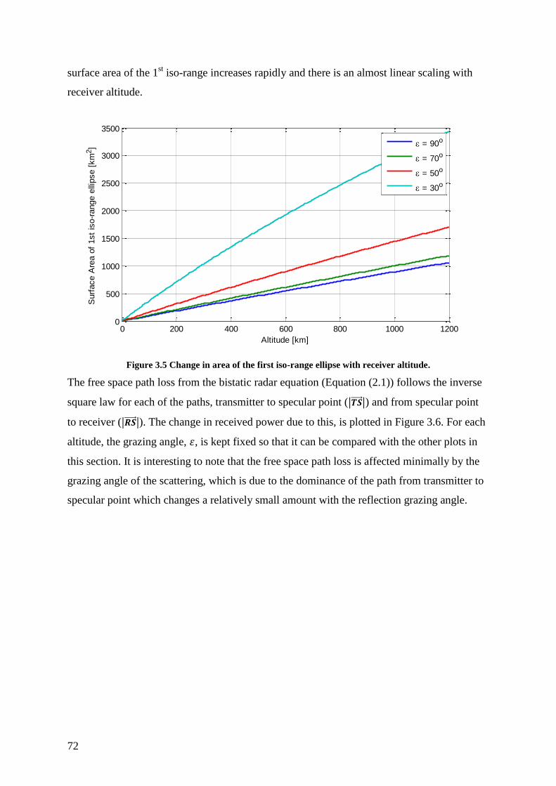
72
surface area of the 1st iso-range increases rapidly and there is an almost linear scaling with
receiver altitude.
Figure 3.5 Change in area of the first iso-range ellipse with receiver altitude.
The free space path loss from the bistatic radar equation (Equation (2.1)) follows the inverse
square law for each of the paths, transmitter to specular point (|𝑻𝑺⃗⃗⃗⃗ ⃗|) and from specular point
to receiver (|𝑹𝑺⃗⃗⃗⃗ ⃗|). The change in received power due to this, is plotted in Figure 3.6. For each
altitude, the grazing angle, 휀, is kept fixed so that it can be compared with the other plots in
this section. It is interesting to note that the free space path loss is affected minimally by the
grazing angle of the scattering, which is due to the dominance of the path from transmitter to
specular point which changes a relatively small amount with the reflection grazing angle.
0 200 400 600 800 1000 12000
500
1000
1500
2000
2500
3000
3500
Altitude [km]
Surf
ace A
rea o
f 1st
iso-r
ange e
llipse [
km
2]
= 90o
= 70o
= 50o
= 30o

System Design
73
Figure 3.6 Free space path loss in comparison to 650km altitude
These terms, the footprint area and the free-space path loss are now combined in Figure 3.7.
The overall gain or loss in reflection power is calculated for the 1st iso-range ellipse and
compared to the reference altitude of UK-DMC at 650 km.
For a rise in altitude the reflected power would decrease due to the free-space path loss, but
this is partially balanced by the increase in the selected surface area contributing a greater
number of scatterers.
Figure 3.7 Reflection power change of 1st iso-range ellipse due to altitude
0 200 400 600 800 1000 1200-10
-5
0
5
10
15
20
Altitude [km]
Fre
e S
pace P
ath
Loss /
Gain
Rela
tive t
o 6
50 k
m a
ltitude [
dB
]
= 90o
= 70o
= 50o
= 30o
0 200 400 600 800 1000 1200-5
-4
-3
-2
-1
0
1
2
3
4
5
Altitude [km]
Radar
equation p
ow
er
com
pare
d t
o 6
50km
altitude[d
B]
= 90o
= 70o
= 50o
= 30o

74
3.5. Modernised and Wide-Band GNSS Signals
An additional parameter in the design space is the choice of GNSS signals. The GPS L1 C/A
signal at 1575.42 MHz has received the focus for most GNSS-R research due to the relative
maturity of the signal, and the wide availability of compatible RF components. Galileo,
GLONASS and GPS are all bringing new wide-band signals into operation which bring the
potential of increased range resolution.
The modernised GPS signals and occupied bands are shown in Figure 3.8, the civilian signals
are shown in blue, with the red and green representing the military P(Y) and M codes
respectively. The GPS C/A signal is the blue signal in the L1 band, with a narrow 2.046 MHz
bandwidth.
The Galileo signals are shown in Figure 3.9. The open service signals in blue, public
regulated service in red and the commercial ones in green. In particular the 51 MHz main-
lobe bandwidth of the E5a/E5b signal would provide a significant increase in range resolution
over the GPS L1 C/A signal. The shape of the spectral density varies between signals
depending on the modulation, and hence the signal AF, although the modulation type will be
ignored at present.
1575.42
MHz
1215
MHz
1237
MHz
L1
1227.6
MHz
L2
1563
MHz
1587
MHz1164
MHz
1189
MHz
L5
1176.45
MHz
Figure 3.8 Band usage of the modernised GPS (courtesy of [Weiler 2009])
1575.42
MHz
1260
MHz
1300
MHz
E2 - L1 - E1
1278.75
MHz
E6
1559
MHz
1591
MHz
1164
MHz
1215
MHz
E5a/E5b
1191.795
MHz
Figure 3.9 Band usage of Galileo (courtesy of [Weiler 2009])

System Design
75
Any radar system strives for the maximum possible bandwidth to achieve the greatest time
resolution, although none of these signals provide the bandwidth of ocean altimeters which
typically have bandwidths in excess of 300 MHz [Zelli & Aerospazio 1999].
The GNSS signals are specified to provide different transmission power. The minimum user
received power is guaranteed in the Interface Control Documents of each of the GNSS. (L1,
L2 in [IS-GPS-200], L5 in [IS-GPS-705] and Galileo in [Galileo OS SIS ICD]).
Table 3.1 GNSS system signal specification
Signal Minimum received
power (dBW) Bandwidth
null to null (MHz)
GPS L1 C/A -158.1 2
GPS L2 -163.1 2
GPS L5 -157.9 40
Galileo E1 B+C -159.1 4
Galileo E5 a+b -155 51
Generally the received power levels of the GPS satellites are between 1 and 5 dB greater than
the specified minimum power levels [Kaplan 2006]. As the power level varies from satellite
to satellite [Fisher & Ghassemi 1999], it can be seen that each of the signals are roughly
equivalent in transmission power, excepting the L2 signal which may be 5 dB weaker than
GPS L1 C/A.
As there are different modulations used in GNSS, here an effective code chip rate will be
used, which is that for an equivalent pseudo-random BPSK signal occupying the same main-
lobe (or null-to-null) bandwidth.
For a BPSK signal, the effective time of a code chip, 𝑇𝑐, is related to the main-lobe
bandwidth 𝑊, by 𝑇𝑐 = 2/𝑊. The wide-bandwidth signals will have a shorter chip time and
therefore the surface resolution will improve, through a reduction in the AF size. The
function 𝜒(𝛥𝑡, 𝛥𝑓), from Equation (2.10), has the width in the delay dimension being a
function of the chip rate 𝑇𝑐.
From our simple model of scattering in the 1st iso-range ellipse, the resolution as a function of
bandwidth can be estimated. The width of the surface ellipse for the 1st code chip is 2 𝑎 and
2 𝑏. The width for a range of scattering geometry is shown in Figure 3.10, which shows the
improvement in ground resolution from 27.4 km with GPS L1 C/A to 5.4 km with Galileo
E5a+b, for a nadir reflection viewed from a 650 km altitude receiver.
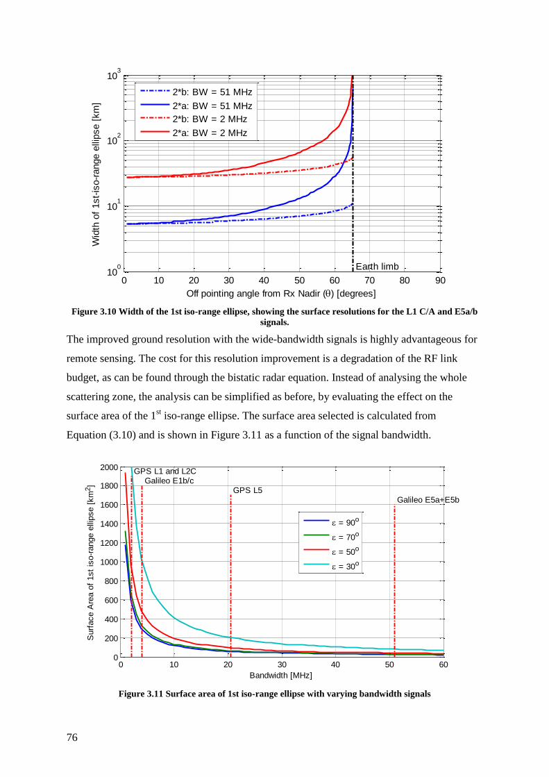
76
Figure 3.10 Width of the 1st iso-range ellipse, showing the surface resolutions for the L1 C/A and E5a/b
signals.
The improved ground resolution with the wide-bandwidth signals is highly advantageous for
remote sensing. The cost for this resolution improvement is a degradation of the RF link
budget, as can be found through the bistatic radar equation. Instead of analysing the whole
scattering zone, the analysis can be simplified as before, by evaluating the effect on the
surface area of the 1st iso-range ellipse. The surface area selected is calculated from
Equation (3.10) and is shown in Figure 3.11 as a function of the signal bandwidth.
Figure 3.11 Surface area of 1st iso-range ellipse with varying bandwidth signals
0 10 20 30 40 50 60 70 80 9010
0
101
102
103
Off pointing angle from Rx Nadir () [degrees]
Wid
th o
f 1st-
iso-r
ange e
llipse [
km
]
Earth limb
2*b: BW = 51 MHz
2*a: BW = 51 MHz
2*b: BW = 2 MHz
2*a: BW = 2 MHz
0 10 20 30 40 50 600
200
400
600
800
1000
1200
1400
1600
1800
2000 GPS L1 and L2C Galileo E1b/c
GPS L5 Galileo E5a+E5b
Bandwidth [MHz]
Surf
ace A
rea o
f 1st
iso-r
ange e
llipse [
km
2]
= 90o
= 70o
= 50o
= 30o
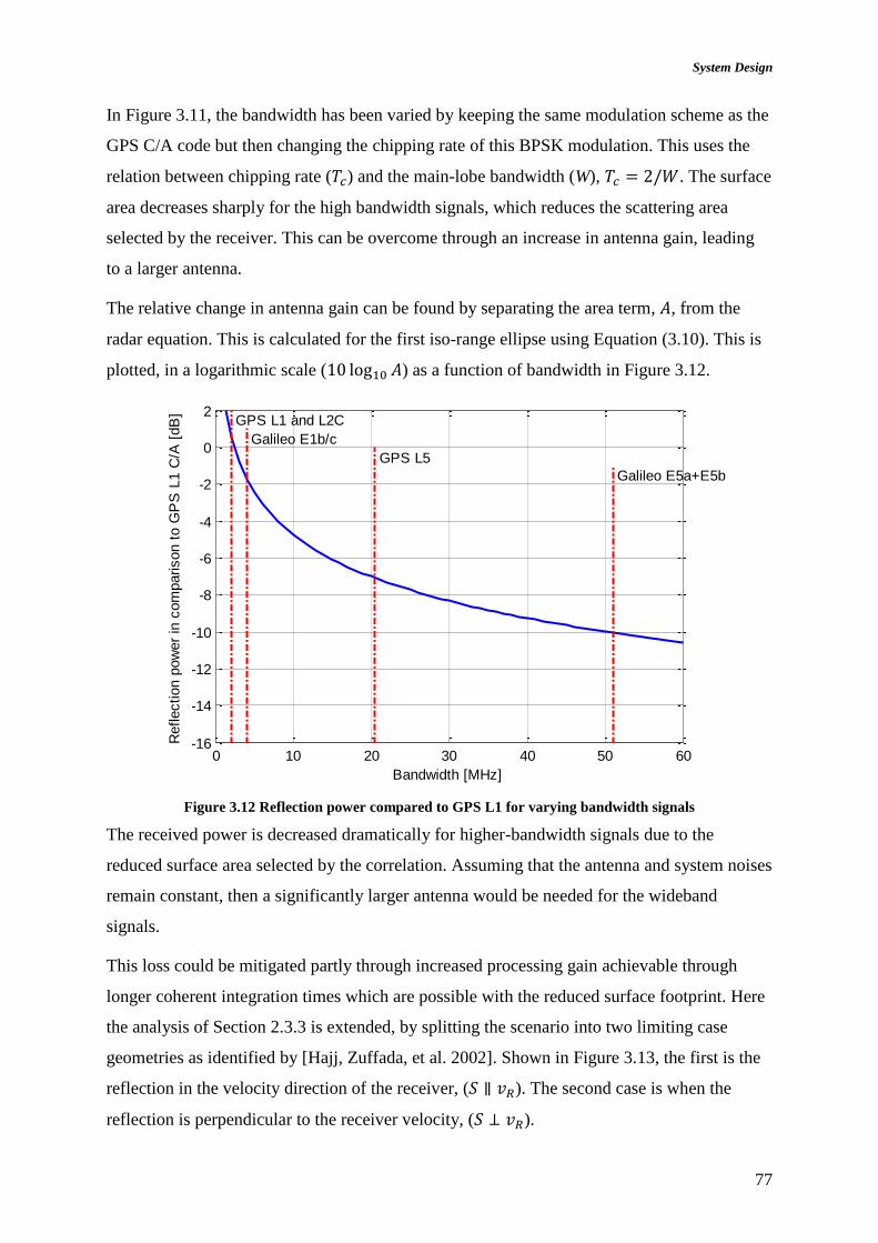
System Design
77
In Figure 3.11, the bandwidth has been varied by keeping the same modulation scheme as the
GPS C/A code but then changing the chipping rate of this BPSK modulation. This uses the
relation between chipping rate (𝑇𝑐) and the main-lobe bandwidth (W), 𝑇𝑐 = 2/𝑊. The surface
area decreases sharply for the high bandwidth signals, which reduces the scattering area
selected by the receiver. This can be overcome through an increase in antenna gain, leading
to a larger antenna.
The relative change in antenna gain can be found by separating the area term, 𝐴, from the
radar equation. This is calculated for the first iso-range ellipse using Equation (3.10). This is
plotted, in a logarithmic scale (10 log10 𝐴) as a function of bandwidth in Figure 3.12.
Figure 3.12 Reflection power compared to GPS L1 for varying bandwidth signals
The received power is decreased dramatically for higher-bandwidth signals due to the
reduced surface area selected by the correlation. Assuming that the antenna and system noises
remain constant, then a significantly larger antenna would be needed for the wideband
signals.
This loss could be mitigated partly through increased processing gain achievable through
longer coherent integration times which are possible with the reduced surface footprint. Here
the analysis of Section 2.3.3 is extended, by splitting the scenario into two limiting case
geometries as identified by [Hajj, Zuffada, et al. 2002]. Shown in Figure 3.13, the first is the
reflection in the velocity direction of the receiver, (𝑆 ∥ 𝑣𝑅). The second case is when the
reflection is perpendicular to the receiver velocity, (𝑆 ⊥ 𝑣𝑅).
0 10 20 30 40 50 60-16
-14
-12
-10
-8
-6
-4
-2
0
2 GPS L1 and L2C
Galileo E1b/c
GPS L5
Galileo E5a+E5b
Bandwidth [MHz]
Reflection p
ow
er
in c
om
parison t
o G
PS
L1 C
/A [
dB
]

78
Figure 3.13 Plan view onto Earth surface of two limiting case geometries for coherence time
determination.
For the receiver to recover all the reflected power from the iso-range ellipse, the coherent
integration time must be set so there is sufficient bandwidth for the range of Doppler
frequencies within the ellipse.
In the 𝑆 ∥ 𝑣𝑅 case the bandwidth of the 1st iso-range ellipse is driven by the major axis size,
2𝑎. In the 𝑆 ⊥ 𝑣𝑅 case the bandwidth of the 1st iso-range ellipse is driven by minor axis size,
2𝑏.
The Doppler shifts are analysed in [Hajj, Zuffada, et al. 2002]. Firstly the 𝑆 ∥ 𝑣𝑅 case, two
points on the surface separated by the distance 2𝑎 will have a Doppler shift separation of
𝐵∥ =
2𝑎
𝜆sin 휀 (
𝑣𝑅 𝑐𝑜𝑠 𝜃
|𝑹𝑺⃗⃗⃗⃗ |−
𝑣𝑇 cos 𝜃𝑇
|𝑻𝑺⃗⃗⃗⃗ | )
(3.11)
For the 𝑆 ⊥ 𝑣𝑅 case, the Doppler shift separation will be
𝐵⊥ =
2𝑏 𝑣𝑅
𝜆 |𝑹𝑺⃗⃗⃗⃗ |
(3.12)
For these, the velocity due to the GPS transmitter motion is minimal so has been ignored. The
coherent integration times to achieve the bandwidth is determined by the relation 𝑇𝑐𝑜ℎ =
2/𝐵, for non-windowed filtering. This results in the coherence time of the 1st iso-range
ellipse shown in Figure 3.14. Both the limiting cases are shown, so that the general geometry
is expected to lie between the two extremes. The widest bandwidth of the GNSS signals

System Design
79
E5a/b is shown alongside the commonly used GPS L1 C/A and the wavelength of these
signals used in the calculation of the coherence times.
Figure 3.14 Coherence time for L1 and E5 signals with angle of specular point from receiver’s nadir. (650
km altitude receiver)
The receiver concept studied here will be targeting reflections away from the Earth limb,
which is the region of validity of the scattering models previously introduced. Effectively the
wide bandwidth E5a+b signal allows an increase in the coherent integration time to 6 ms
under the reasonable assumption that the ocean surface remains essentially static for this
time.
If the receiver will accumulate the signal for a total time 𝑇𝑖𝑛𝑐𝑜ℎ, which is made up of a
number of short coherent integrations, each of duration 𝑇𝑐𝑜ℎ, then the number of coherent
integrations will be 𝑇𝑖𝑛𝑐𝑜ℎ/𝑇𝑐𝑜ℎ. This means that the processing gain has a scaling with
coherence time of
𝐺𝑃 = 𝑇𝑐𝑜ℎ√𝑇𝑖𝑛𝑐𝑜ℎ
𝑇𝑐𝑜ℎ= √𝑇𝑐𝑜ℎ 𝑇𝑖𝑛𝑐𝑜ℎ
(3.13)
0 10 20 30 40 50 60 70 80 900
2
4
6
8
10
12
Off pointing angle from Rx Nadir () [degrees]
Cohere
nce t
ime (
Tcoh)
[ms]
Earth limb
S v, E5, BW = 51 MHz = 0.26 m
S || v, E5, BW = 51 MHz = 0.26 m
S v, L1 C/A, BW = 2 MHz = 0.19 m
S || v, L1 C/A, BW = 2 MHz = 0.19 m

80
The effect of this processing gain is shown in Figure 3.15 for the 650 km satellite with nadir
reflection scenario. This does not take into account the differences in wavelength between the
different GNSS signal options which, additionally affects the coherence time. For L1 to E5
this is 10 log10(𝜆𝐿1/𝜆𝐸5) = 1.3 dB.
Figure 3.15 Processing gain change through exploiting coherence time increase in comparison to those of
2 MHz bandwidth. Wavelength fixed at 0.19 m.
The total reflection power as related to the signal bandwidth is now shown in Figure 3.16.
This includes both the detrimental effect on the surface area when increasing the bandwidth
and the recovery of some of the power through increasing the coherent integration time.
Figure 3.16 Reflection power compared to GPS L1 for varying bandwidth signals. Including processing
gain from variation in coherence time.
0 10 20 30 40 50 600
0.5
1
1.5
2
2.5
3
3.5
4
GPS L1 and L2C Galileo E1b/c
GPS L5 Galileo E5a+E5b
Bandwidth [MHz]
Pro
cessin
g p
ow
er
gain
copm
are
d t
o 2
MH
z B
W [
dB
]
0 10 20 30 40 50 60-16
-14
-12
-10
-8
-6
-4
-2
0
2 GPS L1 and L2C
Galileo E1b/c GPS L5
Galileo E5a+E5b
Bandwidth [MHz]
Pow
er
Gain
/ L
oss in c
om
parison t
o G
PS
L1 C
/A [
dB
]

System Design
81
In conclusion, the L5 and E5, wide-band signals are expected to require an antenna gain
increase of around 6 dB over the baseline receiver specification. The Galileo E1 B and C
signals are good candidate for GNSS-R on a small satellite due to the transmission power and
bandwidth providing a suitable link-margin. The impact of using this signal is investigated in
Section 4.5. By using a suitable antenna gain any of these signals become accessible for
GNSS-R, so the impact of the antenna gain choice is now shown.
3.6. Antenna Gain and Coverage
For a small-satellite launch the orbital altitude may not be within the influence of the receiver
designer. This is particularly the case for technology demonstration or piggy-back missions
that will be likely to share a satellite platform with other payloads. The antenna gain is the
only remaining variable for control of the link budget by the instrument designer.
It is clear that an optimal antenna needs to simultaneously point a high gain directly at each
of the multiple reflection points. This is an ideal application for beam-forming techniques,
although the complexities of the implementation rapidly increase size and cost of the
receiver. In the scope of this project the goal is a demonstration mission, which need only use
a single, fixed beam antenna to accomplish the objectives. If a single fixed antenna is used, as
on UK-DMC and TDS-1, then a higher gain means stronger signals but fewer reflections
enter the beam width. A basic analysis of the trade-off between antenna gain and coverage for
a fixed beam antenna will be carried out.
We will assume that the GNSS satellites are uniformly distributed over the sphere so that the
average number of simultaneous reflections can be determined from the solid angle covered
by the antenna system.
With reference to the geometry described in Figure 3.4, this has been extended in Figure 3.17
to move the transmitter further round its orbit, such that the original specular point, S, moves
further away from nadir so that it becomes S’. This causes a change, at the receiver, of the
off-pointing angle by Δ𝜃. This small change in off-pointing at the receiver corresponds to the
larger change, ΔΘ, in the location of the transmitter (T to T’).

82
Figure 3.17 Geometry of angles subtended at receiver translated into transmitter position
Repeating the work in [Hajj, Zuffada, et al. 2002], the solid angle of transmitters visible to a
nadir pointing antenna subtending Δ𝜃 from nadir, is the integration over all azimuths,
Ω = ∫ ∫ sinΘ𝑑Θ𝑑𝜙
Θ=ΔΘ
Θ=0
2𝜋
𝜙=0
(3.14)
with Θ and ΔΘ found from 𝜃 and Δ𝜃 using Equation (3.7).
Assuming that the GNSS satellites are distributed uniformly over the full sphere, then the
average number of specular points within the receiver’s antenna beam is,
⟨NS⟩ =
NGNSS Ω
4 𝜋
(3.15)
where NGNSS are the total number of GNSS transmitters.
This assumption of uniformly distributed GNSS transmitters is not very good when taken for
an instant in time. This is because the GNSS transmitters have inclined orbits, so do not travel
over the Earth’s poles. (The inclination is 55𝑜 in GPS, 56𝑜 in GALILEO, 64.8𝑜 in
GLONASS, and 55.5𝑜 in COMPASS.) The second issue is that as the GNSS satellites are
arranged in orbital planes, which intersect, causing a greater concentration around the
intersections. The assumption is however useful for determining the average number of
specular reflections over long periods of time.

System Design
83
If we take NGNSS = 32, which has been the reasonably stable number of operational GPS
transmitters during the course of this project, then we can plot ⟨NS⟩ for a range of antenna
beam widths, Figure 3.18. The antenna is characterised by the Half Power Beam Width
(HPBW), where HPBW = 2 Δ𝜃.
Figure 3.18 Average number of simultaneous reflections for nadir pointing antenna with range of
antenna HPBW
To relate antenna gain to HPBW, the relationship for a parabolic antenna will be used as this
has a set of well understood beam and gain characteristics. For other antenna systems suitable
corrections can be applied to these results. The gain of a parabolic antenna [Bakshi, Bakshi,
et al. 2009] is
𝐺 = 10log10 (6 𝑑2
𝜆2 ) dBi (3.16)
where d is the diameter of the reflector, 𝜆 is the RF wavelength. The HPBW is the angular
separation between points in the antenna pattern where the power drops to -3 dB of the
maximum. For parabolic antennas, the HPBW is,
𝐻𝑃𝐵𝑊 = 𝑘𝜆/𝑑 (3.17)
where k is a factor that varies slightly depending on the antenna feed pattern, but for a
‘typical’ parabolic antenna is 70 when the HPBW is expressed in units of degrees.
0 10 20 30 40 50 60 70 80 90 1000
2
4
6
8
10
Antenna HPBW [degrees]
Avera
ge s
imultaneous r
eflections
Receiver altitude = 600 km
Receiver altitude = 700 km
Receiver altitude = 800 km
Receiver altitude = 900 km
Receiver altitude = 1000 km

84
Combining (3.16) and (3.17), then,
𝐻𝑃𝐵𝑊 = 𝑘 √6 (10𝐺/10)⁄ degrees (3.18)
Now the number of reflections with our approximation of the antenna gain can be plotted,
(Figure 3.19). Considering that the antenna gain on the experimental UK-DMC satellite was
11.6 dBi, any increase in antenna gain would adversely affect the coverage.
Figure 3.19 Number of simultaneous reflections with antenna gain for parabolic antenna
By using a fixed antenna beam of 12 dB the system suffers a drop to around 25% of the
ground sampling rate of a multi-beam antenna array, with off-pointing capability of 42o
(equivalent to HPBW of 84o). A simple receiver can make up for the short-fall from the fixed
single-beam antenna by adding the capability to target more GNSS constellations, such as
GLONASS and Galileo as well as GPS. This could approximately triple the average number
of simultaneous reflections from that assumed here. A lower antenna gain would increase the
average number of reflections in view, but with the drawback that the SNR would drop, and
so reduce the accuracy of reflection power measurement..
3.7. Discussion
In conclusion of the system design study, the chosen method for analysis of the link budget
was to make quantified modifications to the scenario used in the UK-DMC GNSS-R
experiment. This provides a greater confidence in the RF link budget by providing scaling of
the received power from the known point of the UK-DMC experiment. By scaling the
5 6 7 8 9 10 11 12 13 14 150
1
2
3
4
5
6
7
8
Antenna Gain [dBi]
Avera
ge s
imultaneous r
eflections
Receiver altitude = 600 km
Receiver altitude = 700 km
Receiver altitude = 800 km
Receiver altitude = 900 km
Receiver altitude = 1000 km

System Design
85
parameters in the link budget using the radar equation model, more confidence can be gained
than relying on the absolute value of the scattering cross-section models.
The effects of the orbital altitude and signal bandwidth has been analysed so that a receiver
can have the antenna gain appropriately scaled to maintain the RF link budget.
The altitude can be varied from 400 km to 1000 km with only a ±2 dB change in antenna
gain. This is due to the change in FSPL being partially cancelled out by the change in the
surface area selected by the ambiguity function.
The change to using different signals from the GPS L1 C/A code used in the UK-DMC
experiment pose a greater effect on the link budget. The wideband signals were found to
reduce the size of the surface footprint and so reduce the received power. This drop in the
received power is not significantly compensated by the processing-gain increase possible
from the increase in coherence time. Therefore a greater antenna gain would be necessary,
which would reduce the coverage. This makes the wideband signals inappropriate for a small
satellite receiver that uses a single, fixed antenna beam.
For the demonstration mission the GPS L1 and Galileo E1 B+C signals shall be the focus of
the system design, as emission power is suitable for the chosen trade-off between coverage
and gain achievable with a fixed-beam antenna.

86
Chapter 4: Tools and Techniques for GNSS-R
From the background and system design a number of critical areas were identified that
required a solution for a spaceborne GNSS-R instrument to be feasible as a secondary
payload or a small satellite payload. These were: improving the link-budget to overcome the
weak GNSS signals, reducing the data rate by on-board processing and the demonstration of
inversion techniques.
To approach these problems a software receiver was developed for post-processing data. This
software receiver provides a test-bench for new receiver techniques which can then be
verified on real data from space, from the UK-DMC GNSS-R experiment. This chapter
describes the design of the software receiver, and some of the techniques that were developed
using it:
Calculation of specular point location
Methods were investigated for the determination of the specular point position
from that of the receiver and transmitter. Particular focus of this section is on
real-time calculation to enable processing GNSS reflections on-board the
receiver. Contributions include improvements to the precision and
computational complexity of calculation.
Modernised signals
Methods developed to use Galileo signal for GNSS-R. New contributions
include overcoming the extended code length and combinations to increase the
received signal power when using combinations of the Galileo sub-codes.
Stare processing
A technique for GNSS-R surface roughness measurement is developed that
does not require calculation of the full DDM. This is applied to the
experimental data from the UK-DMC GNSS-R experiment and the method is
extended to correct for the changing geometry during the measurement period.
Scattering cross-section measurement
A calibration technique is developed for determining absolute scattering cross-
section from a GNSS-R receiver. The method developed is shown to be
suitable for commercial, low cost, GNSS radio down-conversion chips.

Tools and Techniques for GNSS-R
87
4.1. MATLAB Software Receiver System Description
The software receiver was developed within the MATLAB environment and is based on the
book and accompanying software, “A Software-Defined GPS and Galileo Receiver: A
Single-Frequency Approach” [Borre, Akos, et al. 2006]. The software has been extended to
provide a platform for developing GNSS-R processing approaches.
The software receiver flow, as shown in Figure 4.1, uses the direct signals to form a
navigation solution. This is then used to predict the specular point location and steer the
reflection correlators to the predicted delay and Doppler. This is called geometric tracking
and is open-loop as it does not rely on any measure the reflection’s actual tracking offset.
The process flow starts with IF raw samples from an upward (zenith) pointing antenna. The
standard navigation approach of acquisition followed by tracking is performed. The raw files
captured from UK-DMC are only 20 seconds in length, which means that the broadcast
ephemeris is incomplete. The software receiver downloads the missing sub frames from the
International GNSS Service (IGS) [IGS 2010]. This provides the information needed for the
navigation solution.
Figure 4.1 Software receiver schematic representation of the GNSS-R processing flow.

88
From the navigation solution, the receiver position is found and the transmitter position is
determined from the ephemerides and from these the reflection’s specular point is then
calculated using a method from Section 4.4. Then the reflection signal parameters of delay
and carrier frequency are geometrically tracked and passed to the open-loop correlators,
which use the raw IF samples captured from the nadir antenna to either generate DDMs or
perform Stare processing (Section 4.6).
The software receiver has a number of capabilities that distinguish it from previous
realisations of GNSS-R receivers.
Supports variable coherent integration time, to allow investigation of the reflection
coherence properties.
By re-tracking the direct signals, no reliance is made of the data taken at the time of
the collection. Without reliance on a database, the reflection signals are validated for
consistency.
The receiver will track all reflections within a data collection irrespective of the SNR,
through open-loop tracking.
Stare processing, an efficient technique that does not require the whole DDM for
surface measurement.
4.2. Reflection Open-loop Tracking
The software receiver from [Borre, Akos, et al. 2006] already performs the acquisition,
tracking and navigation solution. These steps are additionally documented in GNSS texts
such as [Kaplan 2006]. The following describes the approach for determining the time delay
and frequency of the reflected signal from the outputs of the navigation receiver. These are
then used to perform the geometric-tracking of the reflection for which we need the code
phase, code frequency and carrier frequency.
The receiver clock will typically have a time offset from the GPS system time, and the GNSS
transmitter’s atomic clock will additionally be offset from the system time of the GNSS. The
navigation correlators tracking the direct signal are therefore tracking this time-offset signal.
At any measurement instant the correlator code phase will be a measure of the pseudorange,
so called because it is the range determined by multiplying the signal propagation velocity, 𝑐,
by the time difference between the two, non-synchronised, clocks. The measurement contains
(1) the geometric range, (2) the offset due to the difference in time between system time and

Tools and Techniques for GNSS-R
89
the receiver clock and (3) an offset between system time and the transmitter clock. Due to the
different geometric ranges over the direct and reflected paths, the reflected signal at the
measurement epoch, necessarily departed the transmitter before that of the direct signal.
During this time the satellites will have moved and so the transmitter has two relevant
locations, one for each of the two paths to the receiver. This is as shown in Figure 4.2 against
the system time of the GNSS.
Figure 4.2 Timing of signal propagation for direct and reflected rays
The timing relationships are,
𝑇𝑇𝑥𝐷 = System time at which the signal left the satellite (for direct path)
𝑇𝑇𝑥𝑅 = System time at which the signal left the satellite (for reflected path)
𝑇𝑆 = System time at which the signal reflected from the Earth’s surface
𝑇𝑅𝑥 = System time at which both signals reached the receiver
𝛿𝑡 = Advance of the transmitter clock from system time
𝑡𝑅𝑥 = Offset of the receiver clock from system time
𝑹 = Position of receiver at time of measurement
𝑺 = Position of specular point at time of measured signal’s reflection, 𝑇𝑆
𝑻𝑫, 𝑻𝑹 = Position of transmitter at time of transmission for the direct and reflected
rays respectively
𝒄 = speed of light
For the direct signal the geometric range is,
|𝑹𝑻𝑫⃗⃗ ⃗⃗ ⃗⃗ ⃗⃗ | = 𝑐(𝑇𝑅𝑥 − 𝑇𝑇𝑥𝐷 )
(4.1)
And the pseudorange is formed as in the conventional navigation receiver,

90
𝜌𝐷 = 𝑐((𝑇𝑅𝑥 + 𝑡𝑅𝑥) − (𝑇𝑇𝑥𝐷 + 𝛿𝑡))
= 𝑐(𝑇𝑅𝑥 + 𝑇𝑇𝑥𝐷 ) + 𝑐(𝑡𝑅𝑥 − 𝛿𝑡)
= |𝑹𝑻𝑫⃗⃗ ⃗⃗ ⃗⃗ ⃗⃗ | + 𝑐(𝑡𝑅𝑥 − 𝛿𝑡)
(4.2)
For the reflected signal the geometric range is,
|𝑹𝑺𝑻𝑹⃗⃗ ⃗⃗ ⃗⃗ ⃗⃗ ⃗⃗ ⃗| = 𝑐((𝑇𝑆 − 𝑇𝑇𝑥𝑅 ) + (𝑇𝑅𝑥 − 𝑇𝑆))
= 𝑐(𝑇𝑅𝑥 − 𝑇𝑇𝑥𝑅 )
(4.3)
And the pseudorange of the reflected ray is,
𝜌𝑅 = 𝑐(𝑇𝑆 − (𝑇𝑇𝑥𝑅 + 𝛿𝑡) + (𝑇𝑅𝑥 + 𝑡𝑅𝑥) − 𝑇𝑆)
= 𝑐(𝑇𝑅𝑥 + 𝑇𝑇𝑥𝑅 ) + 𝑐(𝑡𝑅𝑥 − 𝛿𝑡)
= |𝑹𝑺𝑻𝑹⃗⃗ ⃗⃗ ⃗⃗ ⃗⃗ ⃗⃗ ⃗| + 𝑐(𝑡𝑅𝑥 − 𝛿𝑡)
(4.4)
A simplification can be made in the case of the transmission time difference (𝑇𝑇𝑥𝐷 − 𝑇𝑇𝑥
𝑅 )
being small. To test this we take a scenario of receiver and transmitter in circular orbits at
700 km and 20,200 km altitude respectively. The largest range difference (|𝑹𝑺𝑻𝑹⃗⃗ ⃗⃗ ⃗⃗ ⃗⃗ ⃗⃗ ⃗| − |𝑹𝑻𝑫⃗⃗ ⃗⃗ ⃗⃗ ⃗⃗ |)
occurs when the receiver is directly below the transmitter. The maximum specular point to
receiver time (𝑇𝑆 − 𝑇𝑅𝑥) is the time for propagation over the receiver altitude, which is
2.3 ms. The maximum transmitter, specular point to receiver time is twice this, 4.7 ms.
The LEO receiver has speed 7.5 km/s which will cause the specular point to move at a speed
of about 6.5 km/s so will move along the surface by 15 m between the reflection and
measurement time. The GNSS transmitter will have speed 3.8 km/s and travel 18 m between
the transmission and reflection time.
These would be significant if the receiver application were surface altimetry, where the aim is
to measure the surface height to centimetre accuracy. However as the focus of this research is
on scatterometry, these distances are a fraction of a chip length and so we can treat 𝑺 to be at
the measurement time and the transmission times to be the same, 𝑻𝑫 = 𝑻𝑹.
It is therefore possible to set the delay of the reflected signal by applying an offset to the code
phase of the navigation correlator as follows,
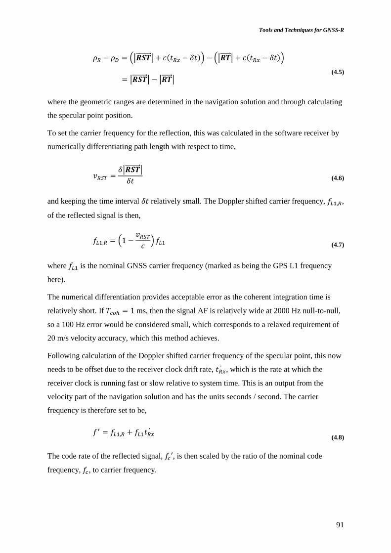
Tools and Techniques for GNSS-R
91
𝜌𝑅 − 𝜌𝐷 = (|𝑹𝑺𝑻⃗⃗ ⃗⃗ ⃗⃗ ⃗⃗ | + 𝑐(𝑡𝑅𝑥 − 𝛿𝑡)) − (|𝑹𝑻⃗⃗ ⃗⃗ ⃗| + 𝑐(𝑡𝑅𝑥 − 𝛿𝑡))
= |𝑹𝑺𝑻⃗⃗ ⃗⃗ ⃗⃗ ⃗⃗ | − |𝑹𝑻⃗⃗ ⃗⃗ ⃗| (4.5)
where the geometric ranges are determined in the navigation solution and through calculating
the specular point position.
To set the carrier frequency for the reflection, this was calculated in the software receiver by
numerically differentiating path length with respect to time,
𝑣𝑅𝑆𝑇 =
𝛿|𝑹𝑺𝑻⃗⃗ ⃗⃗ ⃗⃗ ⃗⃗ |
𝛿𝑡 (4.6)
and keeping the time interval 𝛿𝑡 relatively small. The Doppler shifted carrier frequency, 𝑓𝐿1,𝑅,
of the reflected signal is then,
𝑓𝐿1,𝑅 = (1 −𝑣𝑅𝑆𝑇
𝑐) 𝑓𝐿1
(4.7)
where 𝑓𝐿1 is the nominal GNSS carrier frequency (marked as being the GPS L1 frequency
here).
The numerical differentiation provides acceptable error as the coherent integration time is
relatively short. If 𝑇𝑐𝑜ℎ = 1 ms, then the signal AF is relatively wide at 2000 Hz null-to-null,
so a 100 Hz error would be considered small, which corresponds to a relaxed requirement of
20 m/s velocity accuracy, which this method achieves.
Following calculation of the Doppler shifted carrier frequency of the specular point, this now
needs to be offset due to the receiver clock drift rate, 𝑡𝑅𝑥̇ , which is the rate at which the
receiver clock is running fast or slow relative to system time. This is an output from the
velocity part of the navigation solution and has the units seconds / second. The carrier
frequency is therefore set to be,
𝑓′ = 𝑓𝐿1,𝑅 + 𝑓𝐿1𝑡𝑅𝑥̇ (4.8)
The code rate of the reflected signal, 𝑓𝑐′, is then scaled by the ratio of the nominal code
frequency, 𝑓𝑐, to carrier frequency.

92
𝑓𝑐′ = 𝑓′ ⋅
𝑓𝑐𝑓𝐿1
(4.9)
These code phase, code and carrier frequencies are calculated strictly from the geometry of
receiver, transmitter, and the current clock drift and drift rate in as open-loop tracking and are
calculated periodically steer the DDM processing. The DDM of the reflected signal was then
calculated in the software receiver equivalently to that described in Section 2.3.1.
4.3. Reprocessing UK-DMC Data
The software receiver has been used to re-track all the data-sets that were collected by the
UK-DMC GNSS-R experiment through the work of [Gleason 2006]. Not all of the data-sets
had been processed previously and usually only one reflection per data-set. The geometric
tracking has allowed more reflections to be found in each data set, which greatly increases the
value of the limited number of collections for statistical analysis of the results. An example
set of results has been included in Appendix A for one data collection. This shows how the
reflections are processed through the geometric tracking approach irrespective of the
reflected power level. The value of the barely detectable signals is expected to be in
understanding the detection thresholds rather than determining useful surface measurements.
The work on developing the software receiver has opened the opportunity for new analysis of
these data sets and they are being released for other organisations to analyse. As part of this
process a catalogue of data has been generated from the output of the software receiver. A
shortened version of the catalogue appears in Appendix E.
Most collections were targeted around Hawaii, Figure 4.3, because during the time of the data
collections in 2005 to 2010 there was publically available coincident data from wave buoys
provided by the National Data Buoy Centre [NOAA 2012]. Other areas targeted surfaces
were sea ice in Antarctica and desert in Australia.

Tools and Techniques for GNSS-R
93
Figure 4.3 All UK-DMC data collections where the specular point reflection power is above a detection
threshold
There are 126 specular point tracks where the DDM specular point has a detectable
reflection; this has been defined as a peak power to RMS noise ratio, Equation (2.33), of
greater than 5.
Of particular interest to processing the reflected signals is an effect that was reported in
previous research [Gleason 2006], which was an interference source causing a varying
background noise in the DDM. This was found to be due to a DC bias in the RF front-end and
has been mitigated in the software receiver developed in this work. Further details are given
in Appendix C.
The main focus in this research has been on the processing methods and design of a new
receiver that can collect many times more data than UK-DMC. The software receiver can
also be used to process raw data collections from the SGR-ReSI to verify the new receiver
when it is launched in TDS-1.
Now the remainder of this chapter details the novel contributions to GNSS-R that were
developed with the software receiver. Each part is working towards a critical aspect of the
design of a new real-time instrument for collecting the necessary data for validation of
GNSS-R ocean roughness measurement from space.
4.4. Calculation of the Specular Point Location
Remote sensing for the GNSS-R scatterometry concept tends to focus around the specular
point as this is where the link budget is most favourable for the weak signals. This means that

94
it is necessary to determine the geometric location of the specular point for locating and
tracking the reflected signal in delay and Doppler, and for determining the location of the
targeted area.
Airborne GNSS-R sensors have the advantage that the reflected signal is delayed only by a
few code chips from the direct signal, and the reflected signal is relatively strong. This makes
it relatively easy to locate and track the reflected signals in a similar search approach to that
used for direct signals. The determination of the specular point location is particularly critical
for GNSS-R from space as the reflected signals are weaker and the relative delay is greater.
From the spherical approximation of the geometry in Section 3.3 we can calculate the
difference between the reflected signal path (𝑑 + 𝐷) and the direct path (𝑇𝑅⃗⃗⃗⃗ ⃗), which is
𝑑 + 𝐷 − 𝑇𝑅⃗⃗⃗⃗ ⃗.
To locate the specular point in the signal domain, the delay must be determined to within that
of a single code chip period 𝑇𝑐. The difference in path delay between reflected and direct
paths, in units of code chips is
𝑡 =
𝑑 + 𝐷 − 𝑇𝑅⃗⃗⃗⃗ ⃗
𝑇𝑐 𝑐 (4.10)
where c is the speed of light and 𝑇𝑐 the code chip period.
This can be plotted for the range on grazing angles, 휀, using the geometrical definitions of d,
D and 𝑇𝑅⃗⃗⃗⃗ ⃗ from Section 3.3. The path difference expressed as the number of code chips for a
1.023 MHz chip rate signal and a receiver at 650 km altitude is shown in Figure 4.4. The
grazing angle is plotted between 90 degrees (nadir scattering) and 0 degrees (limb scattering).

Tools and Techniques for GNSS-R
95
Figure 4.4 Difference between direct and reflected path lengths
In this scenario, the search space corresponds to 4300 chips for the GPS L1 C/A code. This
code has PRN length 𝑁𝑐 = 1023 chips, so the search space would fold back to be within
1023 chips. The number of search cells for GPS signal acquisition is 𝑁 = 𝑛 × 𝑁𝑐, where n is
normally 2 [Kaplan 2006] to ensure sufficient sampling density to identify the peak.
As the signals are weak, experience from the UK-DMC experiment tells us that the
integration time for each search cell would be, 𝑁 𝑇𝑐𝑜ℎ where the coherent time of 𝑇𝑐𝑜ℎ ≈
1 𝑚𝑠 and the number of incoherent accumulations N will stretch up-to 1000. This would
result in a dwell time in each search cell of up to 1 second. Without even considering the
additional Doppler search, it is already clear that a ‘cold search’ for the reflected signal is not
practical for over 𝑛 × 1023 search cells with a 1 second dwell. An orbital GNSS-R receiver
would need to calculate the reflection position to aid the search for the reflection.
The purpose of determining the specular point location in the GNSS-R receiver is not just for
initial search for the reflection, but additionally to track the reflection in real-time. In a
conventional navigation receiver the signals are tracked in a closed, delay-locked, loop.
Although a closed loop could be developed for reflection tracking, it was seen as
advantageous to form an open-loop approach which is based on the predicted delay and
Doppler of the calculated specular point location. This allows for tracking to lower signal to
noise ratio levels and resilience to fading which could cause loss-of-lock. Experience has
shown from processing the UK-DMC datasets the occasional occurrence of direct signals
0 10 20 30 40 50 60 70 80 900
500
1000
1500
2000
2500
3000
3500
4000
4500
Angle from incidence vector to surface tangent, [degrees]
Path
diffe
rence:
Reflecte
d -
Direct
[code c
hip
s,
(Tcc
), f
or
GP
S L
1 C
/A]
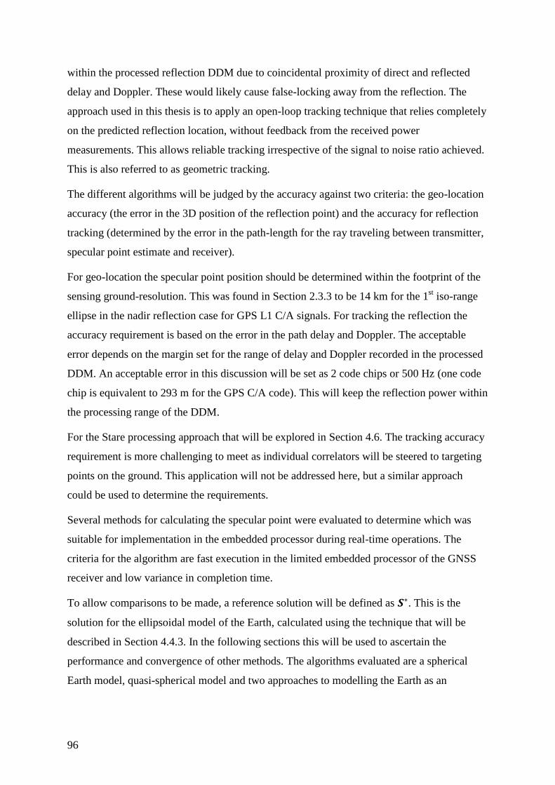
96
within the processed reflection DDM due to coincidental proximity of direct and reflected
delay and Doppler. These would likely cause false-locking away from the reflection. The
approach used in this thesis is to apply an open-loop tracking technique that relies completely
on the predicted reflection location, without feedback from the received power
measurements. This allows reliable tracking irrespective of the signal to noise ratio achieved.
This is also referred to as geometric tracking.
The different algorithms will be judged by the accuracy against two criteria: the geo-location
accuracy (the error in the 3D position of the reflection point) and the accuracy for reflection
tracking (determined by the error in the path-length for the ray traveling between transmitter,
specular point estimate and receiver).
For geo-location the specular point position should be determined within the footprint of the
sensing ground-resolution. This was found in Section 2.3.3 to be 14 km for the 1st iso-range
ellipse in the nadir reflection case for GPS L1 C/A signals. For tracking the reflection the
accuracy requirement is based on the error in the path delay and Doppler. The acceptable
error depends on the margin set for the range of delay and Doppler recorded in the processed
DDM. An acceptable error in this discussion will be set as 2 code chips or 500 Hz (one code
chip is equivalent to 293 m for the GPS C/A code). This will keep the reflection power within
the processing range of the DDM.
For the Stare processing approach that will be explored in Section 4.6. The tracking accuracy
requirement is more challenging to meet as individual correlators will be steered to targeting
points on the ground. This application will not be addressed here, but a similar approach
could be used to determine the requirements.
Several methods for calculating the specular point were evaluated to determine which was
suitable for implementation in the embedded processor during real-time operations. The
criteria for the algorithm are fast execution in the limited embedded processor of the GNSS
receiver and low variance in completion time.
To allow comparisons to be made, a reference solution will be defined as 𝑺∗. This is the
solution for the ellipsoidal model of the Earth, calculated using the technique that will be
described in Section 4.4.3. In the following sections this will be used to ascertain the
performance and convergence of other methods. The algorithms evaluated are a spherical
Earth model, quasi-spherical model and two approaches to modelling the Earth as an

Tools and Techniques for GNSS-R
97
ellipsoid. Finally the analysis will consider the limitations of modelling the real Earth
undulating Earth surface as an ellipsoid.
Monte-Carlo simulations have been performed to determine the performance of the
algorithms. The test cases are created by choosing a random receiver location R, (with
altitude 700 km). A random transmitter location T is then selected (with altitude 20,200 km).
If the transmitter is visible to the receiver (above the Earth limb) then the test case is kept,
otherwise it is replaced with the next generated T.
This creates a scenario with the distribution of transmitter elevation from the receiver as in
Figure 4.5
Figure 4.5 Monte-Carlo elevation distribution for 10,000 runs.
4.4.1. Spherical Earth Approximation
There is a 21 km difference between the Earth’s equatorial and polar radius. The required
accuracy is of the order of one GPS C/A code chip 1 µs (300m). Therefore a better
approximation than spherical will be needed.
If the reflection geometry is simplified to that of a spherical Earth, then the problem can be
specified as that of satisfying the law of reflection, which states that the incident ray and
reflected rays have the same angle to the surface normal. An approach based on the
application of the law of reflection on a spherical earth has been proposed in [Martin-Neira
1993]. The method is used here but not shown and it is suggested that the original work be
-20 0 20 40 60 80 1000
100
200
300
400
500
600
700
800
900
1000Elevation of transmitter from receiver
Elevation (degrees)
His
togra
m f
req.

98
consulted for a thorough explanation. Their method requires solving a quartic polynomial to
determine the specular point position.
The spherical Earth approximation has poor accuracy for locating the reflection, Figure 4.6
(A) shows a maximum of 25 km error in the specular point location for our satellite GNSS-R
scenario. This is calculated at the Euclidean distance between the estimated solution, 𝑺, and
the optimal 𝑺∗. The accuracy is insufficient, particularly, for the tracking of the reflection
delay as the maximum error in path length 𝑅𝑆𝑇⃗⃗⃗⃗⃗⃗ ⃗⃗ is equivalent to 130 times the code ambiguity
function for GPS L1.
(A) (B)
Figure 4.6 Spherical Earth approximation. (A) Distance from solution |S – S*| (B) Distance error in path
𝑹𝑺𝑻⃗⃗ ⃗⃗ ⃗⃗ ⃗⃗
4.4.2. Quasi-Spherical Earth
A quasi-spherical Earth approach can be used to improve the estimate with minimal extra
computation. Using the WGS-84 reference ellipsoid, the Earth is an oblate spheroid with
parameters:
Semi-major axis a = 6,378,137.0 m
Semi-minor axis b ≈ 6,356,752.314245 m
Inverse flattening (1/f) = 298.257223563
An approximation can be made that represents an improvement to the spherical approach.
This manipulation is shown diagrammatically in Figure 4.7.
0 0.5 1 1.5 2 2.5
x 104
0
200
400
600
800
1000
1200Spherical: Euclidean distance between estimates
Distance (m)
His
togra
m f
req.
0 1 2 3 4 5
x 104
0
100
200
300
400
500
600
700
800
900Spherical: Path-length difference
Distance (m)
His
togra
m f
req.
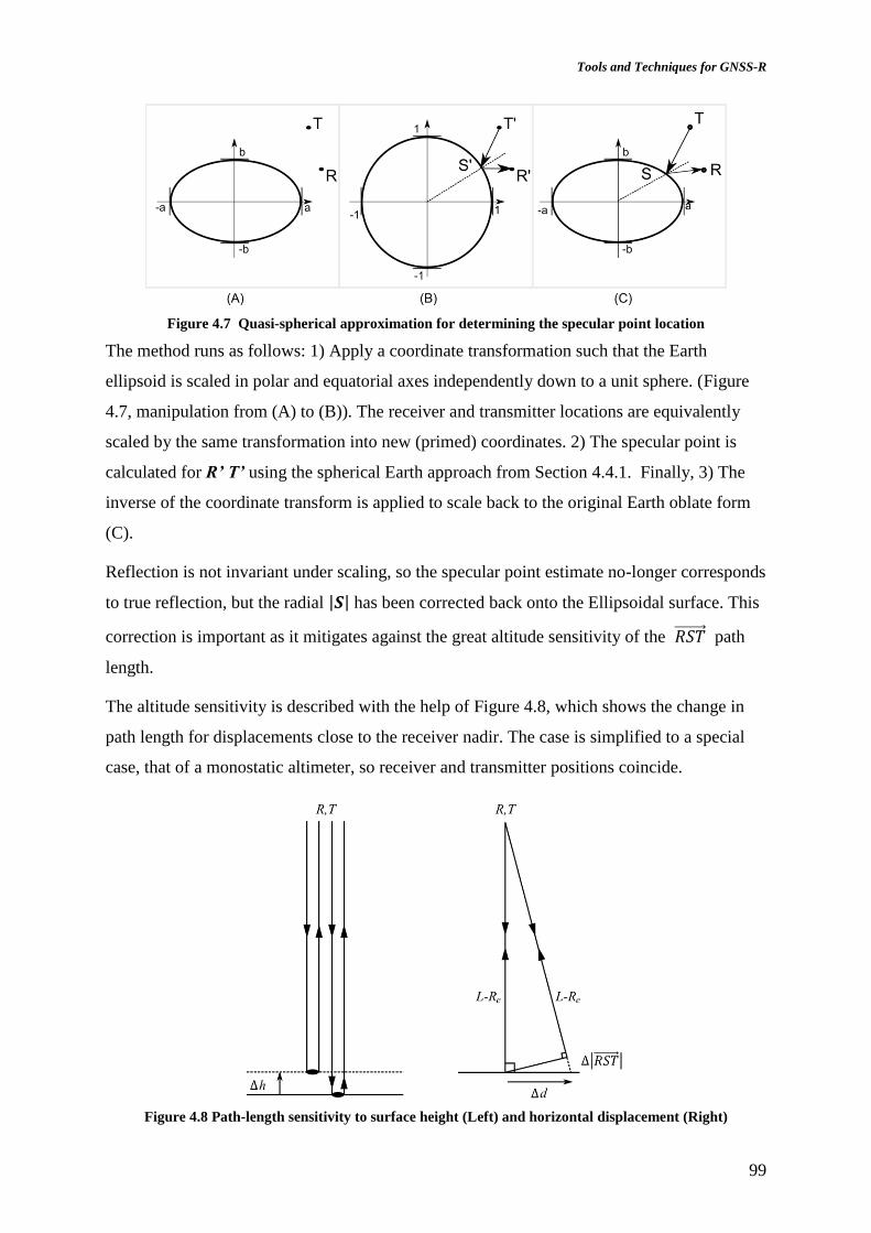
Tools and Techniques for GNSS-R
99
Figure 4.7 Quasi-spherical approximation for determining the specular point location
The method runs as follows: 1) Apply a coordinate transformation such that the Earth
ellipsoid is scaled in polar and equatorial axes independently down to a unit sphere. (Figure
4.7, manipulation from (A) to (B)). The receiver and transmitter locations are equivalently
scaled by the same transformation into new (primed) coordinates. 2) The specular point is
calculated for R’ T’ using the spherical Earth approach from Section 4.4.1. Finally, 3) The
inverse of the coordinate transform is applied to scale back to the original Earth oblate form
(C).
Reflection is not invariant under scaling, so the specular point estimate no-longer corresponds
to true reflection, but the radial |𝑺| has been corrected back onto the Ellipsoidal surface. This
correction is important as it mitigates against the great altitude sensitivity of the 𝑅𝑆𝑇⃗⃗⃗⃗⃗⃗ ⃗⃗ path
length.
The altitude sensitivity is described with the help of Figure 4.8, which shows the change in
path length for displacements close to the receiver nadir. The case is simplified to a special
case, that of a monostatic altimeter, so receiver and transmitter positions coincide.
Figure 4.8 Path-length sensitivity to surface height (Left) and horizontal displacement (Right)
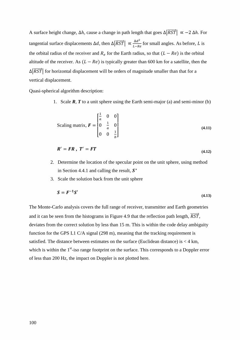
100
A surface height change, Δℎ, cause a change in path length that goes Δ|𝑅𝑆𝑇⃗⃗⃗⃗⃗⃗ ⃗⃗ | ∝ −2 Δℎ. For
tangential surface displacements Δ𝑑, then Δ|𝑅𝑆𝑇⃗⃗⃗⃗⃗⃗ ⃗⃗ | ∝Δ𝑑2
𝐿−𝑅𝑒 for small angles. As before, 𝐿 is
the orbital radius of the receiver and 𝑅𝑒 for the Earth radius, so that (𝐿 − 𝑅𝑒) is the orbital
altitude of the receiver. As (𝐿 − 𝑅𝑒) is typically greater than 600 km for a satellite, then the
Δ|𝑅𝑆𝑇⃗⃗⃗⃗⃗⃗ ⃗⃗ | for horizontal displacement will be orders of magnitude smaller than that for a
vertical displacement.
Quasi-spherical algorithm description:
1. Scale R, T to a unit sphere using the Earth semi-major (a) and semi-minor (b)
Scaling matrix, 𝑭 =
[ 1
𝑎0 0
01
𝑎0
0 01
𝑏]
(4.11)
𝑹′ = 𝑭𝑹 , 𝑻′ = 𝑭𝑻 (4.12)
2. Determine the location of the specular point on the unit sphere, using method
in Section 4.4.1 and calling the result, S’
3. Scale the solution back from the unit sphere
𝑺 = 𝑭−𝟏𝑺′ (4.13)
The Monte-Carlo analysis covers the full range of receiver, transmitter and Earth geometries
and it can be seen from the histograms in Figure 4.9 that the reflection path length, 𝑅𝑆𝑇⃗⃗⃗⃗⃗⃗ ⃗⃗ ,
deviates from the correct solution by less than 15 m. This is within the code delay ambiguity
function for the GPS L1 C/A signal (298 m), meaning that the tracking requirement is
satisfied. The distance between estimates on the surface (Euclidean distance) is < 4 km,
which is within the 1st-iso range footprint on the surface. This corresponds to a Doppler error
of less than 200 Hz, the impact on Doppler is not plotted here.

Tools and Techniques for GNSS-R
101
(A) (B)
Figure 4.9 Quasi-spherical Earth approximation (A) Distance from solution |𝑺 − 𝑺∗| (B) Distance error in
path RST
The localization error is within a fraction of the scale of the ambiguity function in delay and
Doppler so is acceptably small for most needs and has the advantage of being non-iterative
and hence well-suited to a real-time system implementation.
Although this level of accuracy is suitable for meeting the specular point tracking
requirement, it is only just meeting the requirement for the geo-location accuracy. When
additional sources of error are included, such as ephemeris error and atmospheric delays and
deviations from the ellipsoidal surface then the acceptable error will certainly be exceeded
(the additional error sources are quantified in Section 4.4.5). Therefore this accuracy will not
be suitable for all needs so the next section will investigate the improvement through
parameterising the Earth as an Ellipsoid.
4.4.3. Ellipsoidal Earth
To determine the specular point location on the ellipsoidal model of the Earth, the problem
will be expressed as the minimisation of the path length from transmitter to Earth to receiver,
𝑚𝑖𝑛𝑖𝑚𝑖𝑠𝑒 𝑓(𝑺) =∣ 𝑺 − 𝑻 ∣ +∣ 𝑹 − 𝑺 ∣ (4.14)
𝑠𝑢𝑏𝑗𝑒𝑐𝑡 𝑡𝑜 𝑔(𝑺) =
𝑆𝑥2
𝑎2+
𝑆𝑦2
𝑎2+
𝑆𝑧2
𝑏2= 1
(4.15)
0 1000 2000 3000 40000
200
400
600
800
1000
1200
1400Scaled spherical: Euclidean distance between estimates
Distance (m)
His
togra
m f
req.
0 5 10 150
200
400
600
800
1000
1200Scaled spherical: Path-length difference
Distance (m)
His
togra
m f
req.

102
Where a is the equatorial and b the polar radius. The specular point location is S, and the
receiver and transmitter located at R and T respectively. This is a non-linear optimisation
problem with nonlinear constraints. There is not a known analytical solution, although
methods in convex optimisation can be applied to this form of problem [Boyd &
Vandenberghe 2004].
A previous method is given in [Gleason & Gebre-Egziabher 2009] which is based on the
method of steepest descent. This method is analysed here as it is important, but has some
serious short-comings in its present form.
At each iteration, an improved estimate of the specular point location is found along the
direction of the 3D gradient of the path-length function, then constraining the update back
onto the Earth’s surface. From an initial guess of the specular point location 𝑺𝑛, the iterative
procedure is as follows:
1. Take partial differential of path-length function, f(S):
∇𝑓(𝑺𝑛) =
(𝑺𝑛 − 𝑻)
∣ 𝑺𝑛 − 𝑻 ∣−
(𝑹 − 𝑺𝑛)
∣ 𝑹 − 𝑺𝑛 ∣
(4.16)
2. Apply correction to last estimate in direction of derivative, with
update gain K to get a new unconstrained estimate 𝑺′.
𝑺′ = 𝑺𝑛 − 𝐾 ⋅ ∇𝑓(𝑺𝑛) (4.17)
3. Then constrain 𝑺′𝑛+1 to the Earth’s surface, using its radius,
𝑅(𝑺′𝑛+1) beneath the unconstrained solution
𝑺𝑛+1 =
𝑺′
|𝑺′|𝑅(𝑺′)
(4.18)
There are a number of difficulties with this algorithm. The first, as mentioned in [Gleason &
Gebre-Egziabher 2009] is in determining the appropriate update gain K, as the optimum
varies with the geometry of the transmitter and receiver and with the distance of the current
guess away from the correct solution. It is possible to improve on the method by varying K
from iteration to iteration. However this must be carefully done so as not to introduce
unstable limit cycles.

Tools and Techniques for GNSS-R
103
To provide an instance of this algorithm, the value of K has been manually tuned for the
orbital altitudes in the Monte-Carlo test set, and fixed to the value of K = 1,000,000. An
example convergence is given in Figure 4.10. This shows the successive estimates of 𝑺𝒏 as
blue dots plotted with the receiver, R and transmitter, T, sub-satellite points. The contours
show the path length function mapped over the surface. The performance of the algorithm is
shown in Figure 4.11. The solution steps, Sn converge asymptotically.
Figure 4.10 Convergence using constrained steepest descent
Figure 4.11 Convergence of constrained steepest descent to determine specular point location K =
1,000,000
Longitude
Latitu
de
R
T
0 50 100 150 200 250 300 350
-80
-60
-40
-20
0
20
40
60
80
Cost
function:
Path
length
[m
]4.8
5
5.2
5.4
5.6
5.8
6
6.2
6.4x 10
7
5 10 15 20 25 30 35 4010
0
101
102
103
104
105
106
Dis
tance f
rom
S*
[m]
Function Evaluation Number
S

104
The final and most troublesome difficulty is that the method has an intrinsic error introduced
by the process of constraining to the Earth’s surface. This is illustrated in Figure 4.12, where
the flattening of the Earth is exaggerated to demonstrate the problem. In the figure it is
imagined that the correct solution for the location of the specular point has been determined
at 𝑺𝒏. The next iteration will proceed to generate a new unconstrained estimate 𝑺′, which is
then constrained back to the Earth’s surface to create the new estimate 𝑺𝒏+𝟏. The method of
constraining to the ellipsoid surface is to scale back the position vector 𝑺′ to the surface by
the local Earth radial. An error therefore is introduced as a result of the difference between
the surface normal and the radial vectors. This introduces an error unless 𝐾 = 0.
Figure 4.12 Constrained steepest descent, convergence error. Earth flattening exaggerated
The error introduced depends on the magnitude of 𝐾. The error in 𝑺𝒏+𝟏 was found to be up to
60 km for the selected 𝐾. In addition to a position error, this also makes it impossible to set a
reasonable stopping criterion for the iterative algorithm.
The issue can be resolved by projecting the derivative of the cost function ∇𝑓(𝑺𝑛) on to the
constraint surface. This has the effect of linearising the constraints around 𝑺𝑛. Step 2 is
replaced by;
𝑺′ = 𝑺𝑛 − 𝐾 (𝑵 × ∇𝑓(𝑺𝑛)) × 𝑵 (4.19)
Where the surface normal 𝑵 is the derivative of the Earth ellipsoid constraint, ∇𝑔(𝑺𝒏),
defined by the Earth’s equatorial (a) and polar (b)-radii,
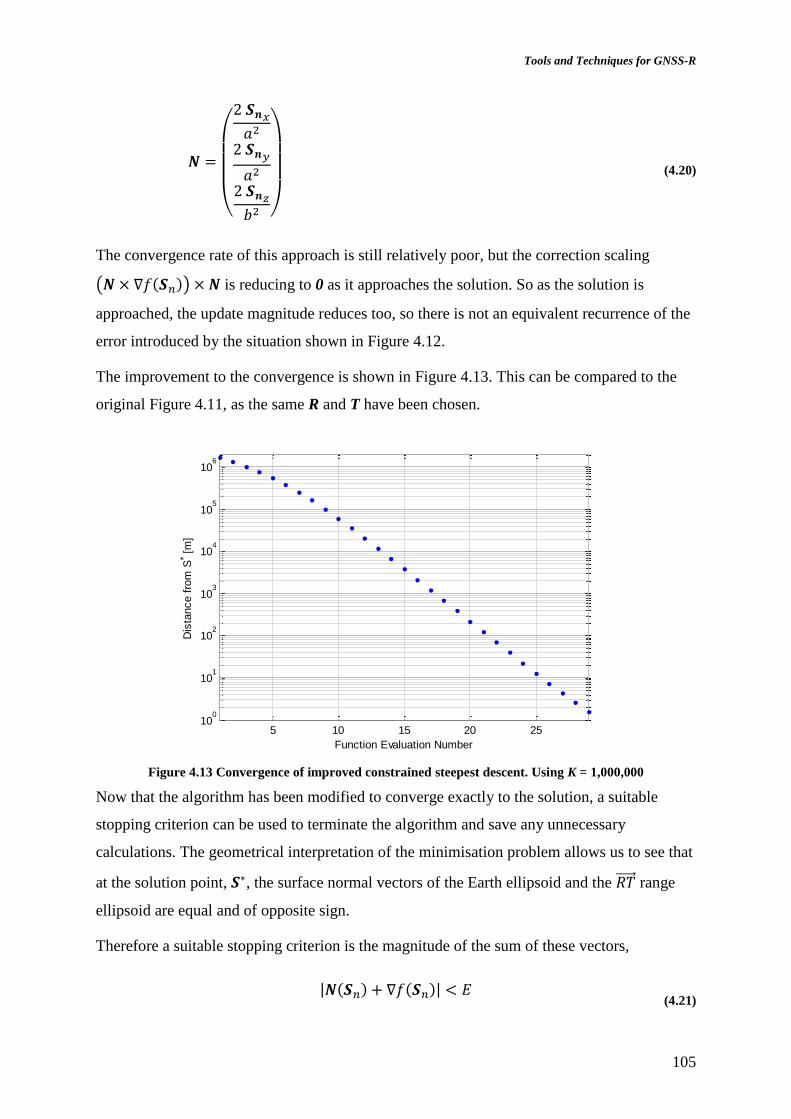
Tools and Techniques for GNSS-R
105
𝑵 =
(
2 𝑺𝒏𝑥
𝑎2
2 𝑺𝒏𝑦
𝑎2
2 𝑺𝒏𝑧
𝑏2 )
(4.20)
The convergence rate of this approach is still relatively poor, but the correction scaling
(𝑵 × ∇𝑓(𝑺𝑛)) × 𝑵 is reducing to 0 as it approaches the solution. So as the solution is
approached, the update magnitude reduces too, so there is not an equivalent recurrence of the
error introduced by the situation shown in Figure 4.12.
The improvement to the convergence is shown in Figure 4.13. This can be compared to the
original Figure 4.11, as the same R and T have been chosen.
Figure 4.13 Convergence of improved constrained steepest descent. Using K = 1,000,000
Now that the algorithm has been modified to converge exactly to the solution, a suitable
stopping criterion can be used to terminate the algorithm and save any unnecessary
calculations. The geometrical interpretation of the minimisation problem allows us to see that
at the solution point, 𝑺∗, the surface normal vectors of the Earth ellipsoid and the 𝑅𝑇⃗⃗⃗⃗ ⃗ range
ellipsoid are equal and of opposite sign.
Therefore a suitable stopping criterion is the magnitude of the sum of these vectors,
|𝑵(𝑺𝑛) + ∇𝑓(𝑺𝑛)| < 𝐸 (4.21)
5 10 15 20 2510
0
101
102
103
104
105
106
Dis
tance f
rom
S*
[m]
Function Evaluation Number

106
Then 𝐸 → 0 as 𝑺𝒏 → 𝑺∗. The value of 𝐸 is not easy to relate to the parameters of interest
either the distance of the location error |𝑺𝒏 − 𝑺∗| or the path length 𝑅𝑆𝑇⃗⃗⃗⃗⃗⃗ ⃗⃗ . It has been found
from analysis of the Monte-Carlo satellite GNSS-R scenario, that if we experimentally
determine a value of 𝐸 such that in the worst case |𝑺𝒏 − 𝑺∗| < 10 m, then some cases will
have been over optimised, and so wasting time, to an accuracy of |𝑺𝒏 − 𝑺∗| < 0.2 m.
To iterate until the worst case error in path-length |𝑅𝑆𝑇⃗⃗⃗⃗⃗⃗ ⃗⃗ | < 1 m, then iteration is required until
𝐸 < 3 ∙ 10−4.
The number of iterations required to reach the stopping criterion of 𝐸 < 3 ∙ 10−6, is shown
for this algorithm in Figure 4.14.
Figure 4.14 Number of iterations required to converge to E < 3*10-6
With minimisation problems, the quality of the initial guess has a great influence on the
number of iterations require to achieve a given accuracy. The simplest initial guess is the
receiver’s sub-satellite point. A better guess is a point 𝑴 which is a weighted distance along
the vector from receiver to transmitter points, this is the approach taken in [Wu, Meehan, et
al. 1997]. This weighted mid-point is then scaled down to the Earth’s surface to get the initial
specular point estimate, 𝑺𝟎.
𝑴 = 𝑹 +
|𝑹|
|𝑹| + |𝑻|(𝑻 − 𝑹)
𝑺𝟎 =𝑴
|𝑴|𝑅𝑒
(4.22)
All the iterative approaches in this section have used this 𝑺𝟎 as the initialisation of the
iterations.
0 20 40 60 80 100 1200
500
1000
1500
2000
2500
3000
Constrained steepest descent: Number of iterations in function minimisation
Number of iterations used
His
togra
m f
req.

Tools and Techniques for GNSS-R
107
4.4.4. Optimisation in Polar Coordinates
A final method will be demonstrated due to its attractive property of being an un-constrained
minimisation. This reduction in complexity is carried out by making the constraint implicit in
the coordinate system. By removing the constraints, it is simple to provide an algorithm to
improve on the asymptotic convergence of the previous methods. Here the polar coordinate
system is used, as first published in [Garrison & Katzberg 1997] and shown in Figure 4.15.
By choosing a polar coordinate system, the position of S can be specified as a pair of angles,
in this case a conventional latitude (𝜙), longitude (𝜆) system.
Figure 4.15 Specular point calculation geometry using polar coordinates (reproduced from [Garrison,
Komjathy, et al. 2002] )
To calculate the path length, the coordinates of S are converted back to the orthogonal basis
𝑺(𝜙, 𝜆) =1
√𝑎2 cos2(𝜙) + 𝑏2 sin2(𝜙)(
𝑎2 ⋅ cos(𝜙) ⋅ cos(𝜆)
𝑎2 ⋅ cos(𝜙) ⋅ sin(𝜆)
𝑏2 ⋅ sin(𝜙)
) (4.23)
This has now changed the problem into one of unconstrained minimisation:
𝑚𝑖𝑛𝑖𝑚𝑖𝑠𝑒 𝑓(𝑺(𝜙, 𝜆)) =∣ 𝑺(𝜙, 𝜆) − 𝑻 ∣ +∣ 𝑹 − 𝑺(𝜙, 𝜆) ∣ (4.24)
which, in general is simpler to solve than a constrained minimisation problem.
There are many computational algorithms for unconstrained minimisation, which are
available from the open literature. Some algorithms are more effective on some problems
than others and some require the gradient ∇𝑓 to be expressible.

108
It is possible to express the gradient of the function, ∇𝑓, however it is computationally
expensive to obtain and needs precision that stretches the standard 64 bit floating point
storage in most modern computers.
A number of algorithms were tested, the results of which are not shown here, but the
conjugate gradient method [Press, Teukolsky, et al. 1992, chap.10.6] was chosen for these
results due to a combination of good convergence performance and relative simplicity. This
approach works on performing minimisation of the cost function over a line from the current
estimate in the direction of steepest descent. After finding the ‘valley floor’ the process
repeats with another line minimisation.
From first inspection it might be thought that the minimisation in polar coordinates may be
unstable due to discontinuities in the coordinate system at the limits of 0 ≤ 𝜙 < 𝜋 and
0 ≤ 𝜆 < 2𝜋, such as when the receiver and transmitter are on different sides of the North or
South pole. The algorithm is stable due to the conversion from polar to linear coordinates
(4.23) being tolerant of overflowing the coordinates thanks to the periodicity of the
trigonometric functions. An iteration step outside of the polar coordinate bounds would still
give a valid conversion to Cartesian. However even though the algorithm is stable
everywhere; it does not have equal performance. This is due to longitude changes subtending
greater surface distances at equatorial latitudes than at high latitudes. This can be seen in the
convergence performance which is better at equatorial latitudes (Figure 4.16) than those
nearer to the poles (Figure 4.17).

Tools and Techniques for GNSS-R
109
Figure 4.16 Equatorial latitude convergence in polar coordinates
Figure 4.17 High latitude convergence in polar coordinate system
Formulation of this method into other coordinate systems is possible, however this method
has the advantage that the derivative of the path length over the coordinate system 𝜕𝑓/𝜕𝜙
and 𝜕𝑓/𝜕𝜆 can be analytically determined. This is not displayed here due to the length of the
resulting expression. The convergence performance has been plotted in Figure 4.18 for the
scenario of receiver and transmitter locations in the Monte-Carlo analysis.
Longitude
Latitu
de
R
T
0 50 100 150 200 250 300 350
-80
-60
-40
-20
0
20
40
60
80
Cost
function:
Path
length
[m
]
4.6
4.8
5
5.2
5.4
5.6
5.8
6
6.2
6.4
6.6x 10
7
Longitude
Latitu
de
R
T
0 50 100 150 200 250 300 350
-80
-60
-40
-20
0
20
40
60
80
Cost
function:
Path
length
[m
]
4.8
5
5.2
5.4
5.6
5.8
6
6.2
6.4x 10
7
S
S
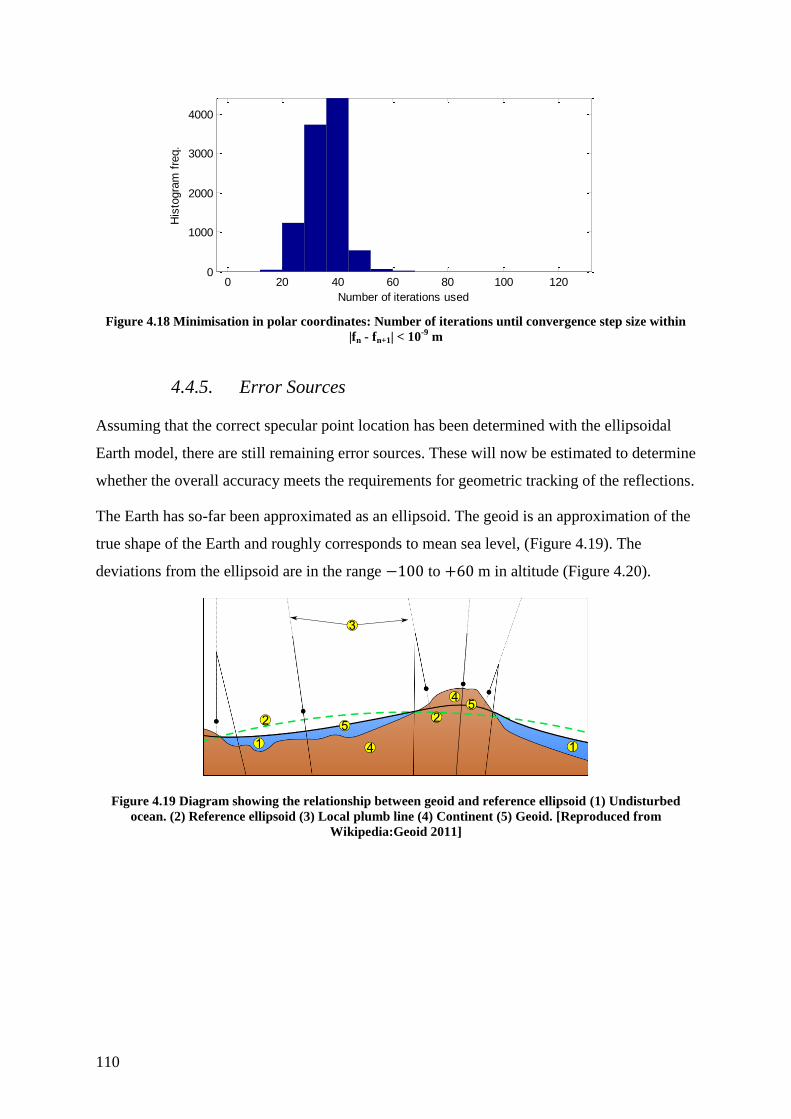
110
Figure 4.18 Minimisation in polar coordinates: Number of iterations until convergence step size within
|fn - fn+1| < 10-9
m
4.4.5. Error Sources
Assuming that the correct specular point location has been determined with the ellipsoidal
Earth model, there are still remaining error sources. These will now be estimated to determine
whether the overall accuracy meets the requirements for geometric tracking of the reflections.
The Earth has so-far been approximated as an ellipsoid. The geoid is an approximation of the
true shape of the Earth and roughly corresponds to mean sea level, (Figure 4.19). The
deviations from the ellipsoid are in the range −100 to +60 m in altitude (Figure 4.20).
Figure 4.19 Diagram showing the relationship between geoid and reference ellipsoid (1) Undisturbed
ocean. (2) Reference ellipsoid (3) Local plumb line (4) Continent (5) Geoid. [Reproduced from
Wikipedia:Geoid 2011]
0 20 40 60 80 100 1200
1000
2000
3000
4000
Conjugate gradient: Number of iterations in function minimisation
Number of iterations used
His
togra
m f
req.

Tools and Techniques for GNSS-R
111
Figure 4.20 Deviation of the EGM96 geoid from the WGS-84 reference ellipsoid [Reproduced from
MathWorks Mapping Toolbox 2012]
Further sources of error include: ephemeris error, tidal movement, delays due to the neutral
and charged atmosphere and receiver hardware delays.
These are covered in standard GNSS texts such as [Kaplan 2006] and are expected to add a
combined error of less than 100 m. The only error term that is not covered sufficiently by
standard texts is the receiver hardware delay.
The path delay within a navigation receiver is commonly ignored as an error source due to
the way in which it self-cancels in the navigation solution. The signal from each GNSS
satellite is delayed as it passes through the receiver components until the point where the
pseudo-range is measured. The absolute group delay may be over 300 ns (corresponding to
90 m) with long antenna cables and or when a SAW (Surface Acoustic Wave) filter is used
[Mitel 1997].
In a navigation receiver, the signal from each transmitting satellite is delayed exactly the
same, as they all pass through the same receiver path, so that when the position solution is
calculated, the common delay comes out in the clock bias term and not the position [Kaplan
2006].
For reflectometry, there is a different path length for the direct and reflected antenna receiver
paths which may need to be calibrated, if the uncertainty is considered too great. The inter-
channel delay can be measured by tracking one signal on both antennas simultaneously. This
calibration was performed using the software receiver on the UK-DMC data to measure the
inter-channel delay. It was found that the delay was smaller than the measurement accuracy
of the software receiver in the UK-DMC experiment, Figure 4.21. This figure shows the
result of running the software receiver in open-loop tracking mode, targeted at the direct
signal from one of the GPS transmitters. The signal is visible in both antennas, from the
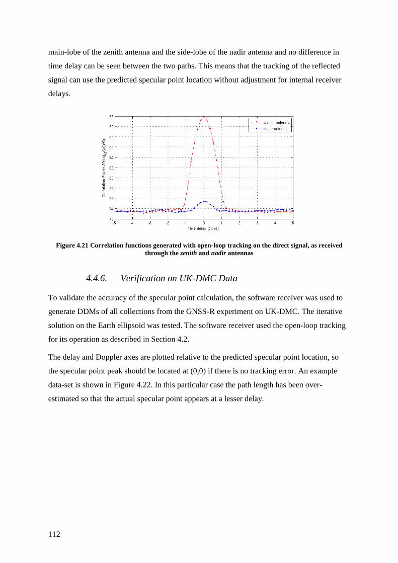
112
main-lobe of the zenith antenna and the side-lobe of the nadir antenna and no difference in
time delay can be seen between the two paths. This means that the tracking of the reflected
signal can use the predicted specular point location without adjustment for internal receiver
delays.
Figure 4.21 Correlation functions generated with open-loop tracking on the direct signal, as received
through the zenith and nadir antennas
4.4.6. Verification on UK-DMC Data
To validate the accuracy of the specular point calculation, the software receiver was used to
generate DDMs of all collections from the GNSS-R experiment on UK-DMC. The iterative
solution on the Earth ellipsoid was tested. The software receiver used the open-loop tracking
for its operation as described in Section 4.2.
The delay and Doppler axes are plotted relative to the predicted specular point location, so
the specular point peak should be located at (0,0) if there is no tracking error. An example
data-set is shown in Figure 4.22. In this particular case the path length has been over-
estimated so that the actual specular point appears at a lesser delay.

Tools and Techniques for GNSS-R
113
Figure 4.22 Power DDM of 'PUR3' data set PRN 1, open-loop tracking aligned to (0,0). 1000 incoherent
accumulations of 1 ms coherent correlations
For each DDM, a cut was taken at 0 Hz Doppler, as shown by the vertical dotted line in
Figure 4.22. This creates a delay map at this constant Doppler frequency. This has been
plotted for the example DDM in Figure 4.23 and from these the timing error 𝛿𝑇 can be
determined.
Figure 4.23 Determining the open-loop tracking error . Delay cut of the DDM. Upper) processed delay
range. Lower) Zoom in around tracking point showing tracking error
Doppler Hz
CA
Code C
hip
s
DDM from: PUR3-Nadir
-1.5 -1 -0.5 0 0.5 1 1.5
x 104
-5
0
5
10
15
20
25
30
35
Sig
nal P
ow
er:
[sta
ndard
devia
tions f
rom
nois
e m
ean]
2
4
6
8
10
12
14
16

114
To measure the tracking timing error, the rising edge of the correlation, the time of half
maximum correlation power, 𝑡𝐸, was used as the reference. This is used rather than the
maximum so that the shortest path delay is measured, incorporating less power leakage from
scatterers in the rest of the 1st iso-range ring. This is shown diagrammatically in Figure 4.24.
This schematic view of the scattering is consistent with the delay maps modelled in
[Zavorotny & Voronovich 2000].
The impulse response of the scattering is expected to be zero for delays before the specular
point delay (physically above) the surface. Following the specular point the impulse function
will depend on surface roughness, so is marked as a number of dotted lines. When the GNSS
signal auto-correlation function, Λ, is convolved with an impulse response, then the best
estimate of the specular point delay corresponds to the rising edge.
Figure 4.24 Convolution of the surface impulse response with the signal ACF
The DDMs produced are power maps rather than magnitude, with AF equal to |Λ|2. So the
half power point corresponds to a delay offset of (1 − √0.5)𝑇𝑐 = 0.3𝑇𝑐, so the timing error in
the open-loop tracking is therefore that read from the delay-map offset by,
𝛿𝑇 = 𝑡𝐸 + 0.3𝑇𝑐
The lower graph enlarges the rising edge, from which the delay of 𝑡𝐸 = −1.8 GPS C/A code
chips is read off. The open-loop tracking error is therefore 𝛿𝑇 = −1.3 chips, or 390 m in this
case.
This procedure for estimating the delay could be used for altimetric measurement of the
surface height, but in this case the aim is validating the specular point calculation and the
open-loop tracking.
For all the UK-DMC data collections the offset of the delay was calculated in this way and
the results are combined in Figure 4.25. For all collections the open-loop tracking used the
ellipsoidal Earth specular point calculation. Some of the datasets included reflections from

Tools and Techniques for GNSS-R
115
the land, which would have a greater surface height. These have not been excluded so will
produce some of the out-lying values. In addition some outliers are due to interference from
the direct signal coinciding within the DDM.
After filtering out the very low reflection SNR data sets, there were 423 remaining DDMs.
These do not all provide independent points, due to the geographical clustering of the data-
sets in the archive and as there will be around 16 DDMs from each data collection (one for
each second of the collection processed).
Figure 4.25 Histogram of open-loop tracking error in UK-DMC data sets. Using ellipsoidal Earth model
The mean path-length error achieved is −444.5 m with standard deviation 664.9 m. This is
1.5 ± 2.2 GPS C/A code chips. The open-loop tracking is meeting the required accuracy to
keep the reflection within the DDM through verification against the true Earth surface and as
real data has been used it includes but does not control all the additional error sources such as
deviation from the ellipsoid, atmospheric delay and satellite ephemeris error.
4.4.7. Discussion
Treating the Earth as a spherical body, the calculation of the specular point location is too
poor for either geo-location or for signal tracking. The spherical approach is still highly
useful for analysis of the general geometry of GNSS-R for analysis of the system design. An
improvement was made in the form of the quasi-spherical Earth approximation. This is fast to
calculate and is non-iterative so has a deterministic calculation time. This new simplification
meets the requirements for tracking the reflection and for DDM processing, as the path-length
-2000 -1000 0 1000 2000 3000 4000 5000 6000 7000 80000
20
40
60
80
100
120
Fre
quency
Path-length error [m]
Histogram of open-loop tracking pathlength error

116
uncertainty is just 15 m from that of the Earth ellipsoid model. The position accuracy at better
than 4 km error also meets the geo-location requirement of 12 km. The quasi-spherical Earth
method is therefore a very good approximation in the case of a LEO receiver.
The two ellipsoidal-Earth methods calculate the correct solution for the specular point on an
ellipsoid, following the improvement to the constrained steepest descent algorithm. The
improvement found in this research improves the geo-location accuracy although there is
further potential to improve the asymptotic convergence rate.
The specular point locations were used for geometric tracking of the reflections on real data
from the UK-DMC GNSS-R receiver. This has verified the specular point calculation
approach and allowed the overall accuracy to be estimated. The geometric tracking allowed
reflections to be tracked reliably even if they are close to the detection limit imposed by
thermal noise.
If the geometric tracking approach were implemented on a real-time GNSS-R receiver then it
would enable on-board processing of the reflections. This was determined as necessary for
the system design to reduce the rate of data to downlink to the ground station. Extension of
the tracking to real-time operation is discussed in Section 5.8.
Through this work many more reflections have been found in the UK-DMC data which allow
better use of the limited data-set available from UK-DMC. For a future instrument more
reflection points results in greater sampling coverage of the Earth’s surface.
4.5. Galileo-Reflectometry
The primary reason for utilising Galileo signals as well as just those available from GPS is
that an increase in the number of transmitters leads to more specular points and greater
coverage available from one receiver.
At the time of this research two test satellites GIOVE-A and GIOVE-B had been operating in
orbit for a number of years and towards the end of the work an additional two In-Orbit
Validation (IOV) satellites were launched, with two more on their way.
The E1 Galileo signals are chosen for investigation as they exhibit some interesting
modulation characteristics that are being introduced in several of the modernised GNSS
signals; also the E1 frequency coincides with GPS L1 so verification is possible using real
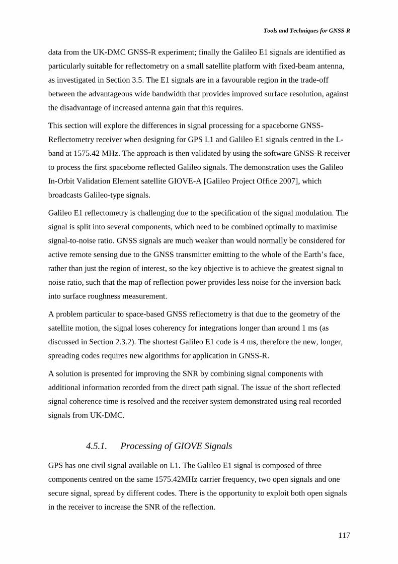
Tools and Techniques for GNSS-R
117
data from the UK-DMC GNSS-R experiment; finally the Galileo E1 signals are identified as
particularly suitable for reflectometry on a small satellite platform with fixed-beam antenna,
as investigated in Section 3.5. The E1 signals are in a favourable region in the trade-off
between the advantageous wide bandwidth that provides improved surface resolution, against
the disadvantage of increased antenna gain that this requires.
This section will explore the differences in signal processing for a spaceborne GNSS-
Reflectometry receiver when designing for GPS L1 and Galileo E1 signals centred in the L-
band at 1575.42 MHz. The approach is then validated by using the software GNSS-R receiver
to process the first spaceborne reflected Galileo signals. The demonstration uses the Galileo
In-Orbit Validation Element satellite GIOVE-A [Galileo Project Office 2007], which
broadcasts Galileo-type signals.
Galileo E1 reflectometry is challenging due to the specification of the signal modulation. The
signal is split into several components, which need to be combined optimally to maximise
signal-to-noise ratio. GNSS signals are much weaker than would normally be considered for
active remote sensing due to the GNSS transmitter emitting to the whole of the Earth’s face,
rather than just the region of interest, so the key objective is to achieve the greatest signal to
noise ratio, such that the map of reflection power provides less noise for the inversion back
into surface roughness measurement.
A problem particular to space-based GNSS reflectometry is that due to the geometry of the
satellite motion, the signal loses coherency for integrations longer than around 1 ms (as
discussed in Section 2.3.2). The shortest Galileo E1 code is 4 ms, therefore the new, longer,
spreading codes requires new algorithms for application in GNSS-R.
A solution is presented for improving the SNR by combining signal components with
additional information recorded from the direct path signal. The issue of the short reflected
signal coherence time is resolved and the receiver system demonstrated using real recorded
signals from UK-DMC.
4.5.1. Processing of GIOVE Signals
GPS has one civil signal available on L1. The Galileo E1 signal is composed of three
components centred on the same 1575.42MHz carrier frequency, two open signals and one
secure signal, spread by different codes. There is the opportunity to exploit both open signals
in the receiver to increase the SNR of the reflection.

118
The three components are each designed to provide a distinct service to the navigational user.
At an application level, the E1A signal will provide a wideband signal for superior precision,
which is secured and unavailable for public use. The open E1B signal provides the navigation
data e.g. ephemeris and satellite status. E1C is also an open signal, providing a pilot tone to
help reception in low signal to noise environments. The E1B and E1C channels are often
known as data and pilot respectively.
The signal definitions for the GIOVE-A signals are specified in the Interface Control
Document (ICD) [Galileo Project Office 2007]. The signals transmitted by the GIOVE-A
satellite are representative of the future Galileo signals with some minor differences.
The design of each GNSS signal has been driven by the aim of best navigational
performance, as GNSS reflectometry is an application distant from the intended use, then
differences between the signals need to be reassessed. The most significant differences when
moving from a GPS L1 receiver to GIOVE-A E1 are the modulation changes from Binary
Phase Shift Keyed (BPSK) to Binary Offset Carrier (BOC), this causes the bandwidth to
almost double. In addition the PRN code length is increased: the GPS C/A code is 1 ms long,
GIOVE-A’s two open codes, E1B and E1C are 4 ms and 8 ms long respectively (the Galileo
full operational constellation has been specified to use 4 ms on both E1B and E1C as well as
some other differences [Galileo Project Office 2010]).
The broadcast signal 𝑠𝐸1(𝑡) is made up of the three sub-signals (E1A, E1B and E1C) and an
intermodulation product, 𝑚𝐸1(𝑡).
𝑠𝐸1(𝑡) = √2 cos(2𝜋𝑓𝐿𝑡) ⋅ (𝑐𝐸1𝐵(𝑡) ⋅ 𝑠𝑐(𝑡) ⋅ 𝑑(𝑡) − 𝑐𝐸1𝐶(𝑡) ⋅ 𝑠𝑐(𝑡) ⋅ 𝑐𝑆(𝑡))
+ 𝑖 √2 sin(2𝜋𝑓𝐿𝑡) ⋅ (2𝑐𝐸1𝐴(𝑡) + 𝑚𝐸1(𝑡)) (4.25)
The carrier at frequency, 𝑓𝐿 = 1.57542 GHz, is modulated with a binary phase shift due to
the modulation terms: 𝑐𝐿1𝐵(𝑡), 𝑐𝐿1𝐶(𝑡), 𝑠𝑐(𝑡), 𝑑(𝑡), 𝑐𝑠(𝑡) ∈ (−1,1).
The E1A component is a secure wideband signal where 𝑐𝐸1𝐴(𝑡) contains its own sub carrier,
data terms and an unpublished code and is on the orthogonal carrier phase to the E1B and
E1C codes. The intermodulation product, 𝑚𝐸1(𝑡), ensures a constant amplitude modulation
before high power amplification on board the satellite.
The open components are modulated using different PRN codes, 𝑐𝐸1𝐵(𝑡) and 𝑐𝐸1𝐶(𝑡), which
for Galileo are stored memory codes, with a sequence specific to each satellite. For the

Tools and Techniques for GNSS-R
119
E1A,B signals the sub carrier term, 𝑠𝑐(𝑡) provides the Binary Offset Carrier (BOC) sub-
modulation. The sine phase BOC(1,1) sub carrier is used, which resembles that shown in the
lower part of Figure 4.26. The effect of the sub-carrier is to broaden the bandwidth of the
signal and thus improve the ranging resolution of the auto-correlation function.
Figure 4.26 BOC(1,1) modulation components. PRN code c(t) and subcarrier sc(t)
In addition to these high-rate modulations, the E1B component is also modulated by the data
bit, 𝑑(𝑡) of 250 symbols per second. The pilot component, E1C, is modulated by a secondary
code 𝑐𝑠(𝑡), which is a 25 chip long sequence that repeats every 200 ms.
The BOC(1,1) modulation has an auto-correlation function compared to GPS L1 is shown in
Figure 4.27. The higher resolution is evident and beneficial in GNSS-R, however the large
side-lobes would usually be considered a problem in radar signal designs.
Figure 4.27 Correlation function of the BOC(1,1) (blue) and BPSK (red) spreading codes.
The code lengths and chipping rates are reproduced here in Table 4.1 for reference, these are
compiled from the GPS and GIOVE-A ICDs [GPS Directorate 2011; Galileo Project Office
2007].

120
Table 4.1 Comparison of GPS and GIOVE signals centred on 1.57542GHz. (Excluding secured signals)
The model of the GNSS-R reflection will be taken from Section 2.2.1 and modified to
represent the E1 signal.
The signal input to the receiver has been distorted by the reflection off the ocean, and is
buried in noise. This shall be modelled as a set of E1 signal sources (𝑠𝐸1(𝑡) from Equation
(4.25)), each distributed over the surface so that they have some phase, 𝜙𝑖, Carrier frequency,
𝑓𝐿, Doppler shift, 𝑓𝐷,𝑖, propagation delay 𝜏𝑖, and amplitude 𝐴𝑖
𝑠𝑟𝑥(𝑡) = ∑ (𝐴𝑖 ∙ 𝑠𝐸1(𝑡 − 𝜏𝑖) ∙ exp(𝑗2𝜋(𝑓𝐿 + 𝑓𝐷,𝑖) + 𝜙𝑖))
𝑖=0,1…
+ 𝑛(𝑡) (4.26)
To bring the signal out from the dominant noise term, n(t), the signal needs to be mixed down
from the Doppler shifted carrier frequency, (𝑓𝐿 + 𝑓𝐷,𝑖), and de-spread by correlating with an
internal replica 𝑠𝐸1. For a navigation receiver, the replica cannot be produced as in Equation
(4.25) for the full 𝑠𝐸1 signal, due to the unknown data bits 𝑑(𝑡) and not necessarily a
synchronised secondary code 𝑐𝑠(𝑡).
The receiver can correlate the combined PRN code and sub-carrier for the B and C channels
separately. This forms the following two correlation results for a ray of the reflected signal,
𝑤𝐸1𝐵(𝑡′, 𝑓′) =
1
𝑇𝑐𝑜ℎ∫ 𝑠𝑟𝑥(𝑡)𝑐𝐸1𝐵(𝑡
𝑇𝑐𝑜ℎ
0
− 𝑡′) 𝑠𝑐(𝑡 − 𝑡′)exp( 𝑗2𝜋(𝑓𝐿 + 𝑓𝐷 − 𝑓′)𝑡 + 𝜙)𝑑𝑡 + 𝑛𝑤,𝐵 (4.27)
Modulation Band-width (null-null)
Code length (chips) Data symbol
rate (bps)
Pilot code rate (Hz)
Power (dBW)
Primary Secondary
GIOVE-A:
E1B BOC(1,1) 4MHz 4092 1 250 N/A 22% of -155.7
E1C BOC(1,1) 4MHz 8184 25 N/A 125 22% of -155.7
GPS:
C/A BPSK 2MHz 1023 1 50 N/A -158.5

Tools and Techniques for GNSS-R
121
𝑤𝐸1𝐶(𝑡′, 𝑓′) =
1
𝑇𝑐𝑜ℎ∫ 𝑠𝑟𝑥(𝑡)𝑐𝐸1𝐶(𝑡 − 𝑡′)𝑠𝑐(𝑡
𝑇𝑐𝑜ℎ
0
− 𝑡′) exp( 𝑗2𝜋(𝑓𝐿 + 𝑓𝐷 − 𝑓′)𝑡 + 𝜙)𝑑𝑡 + 𝑛𝑤,𝐶 (4.28)
using a coherent integration time of 𝑇𝑐𝑜ℎ and trial delay and Doppler of 𝑡′ and 𝑓′
respectively. The post-correlation noises are separated out as 𝑛𝑤,𝐵 and 𝑛𝑤,𝐶 for convenience.
Performing these correlations for a range of trial delays 𝑡’ and Doppler frequencies 𝑓′, builds
up a map of the distortion caused by the reflection and resulting in a coherent DDM as
discussed for the GPS signals in Section 2.3.1. Recovery of the complete signal power from
E1 will be necessary if a GNSS-R receiver is to use Galileo transmitters in addition to GPS to
increase remote sensing coverage.
Focusing in on the modulation terms of the E1B correlation: 𝑠𝑟𝑥(𝑡)𝑐𝐸1𝐵(𝑡 − 𝑡′) 𝑠𝑐(𝑡 − 𝑡′)
and expanding out the received signal,
(𝑐𝐸1𝐵(𝑡 − 𝜏) ⋅ 𝑠𝑐(𝑡 − 𝜏) ⋅ 𝑑(𝑡 − 𝜏) − 𝑐𝐸1𝐶(𝑡 − 𝜏) ⋅ 𝑠𝑐(𝑡 − 𝜏) ⋅ 𝑐𝑆(𝑡 − 𝜏))
⋅ 𝑐𝐸1𝐵(𝑡 − 𝑡′) 𝑠𝑐(𝑡 − 𝑡′) (4.29)
𝑐𝐸1𝐵(𝑡 − 𝜏) ⋅ 𝑠𝑐(𝑡 − 𝜏) ⋅ 𝑑(𝑡 − 𝜏) ⋅ 𝑐𝐸1𝐵(𝑡 − 𝑡′) ⋅ 𝑠𝑐(𝑡 − 𝑡′)
−𝑐𝐸1𝐶(𝑡 − 𝜏) ⋅ 𝑠𝑐(𝑡 − 𝜏) ⋅ 𝑐𝑆(𝑡 − 𝜏) ⋅ 𝑐𝐸1𝐵(𝑡 − 𝑡′) ⋅ 𝑠𝑐(𝑡 − 𝑡′) (4.30)
Inside the integration, we can use the relation that as the E1A, E1B and E1C codes are
different pseudo-random bi-phase sequences, so that for all replica delays, 𝑡′ and propagation
delays 𝜏:
⟨𝑐𝐸1𝐵(𝑡 − 𝜏)𝑐𝐸1𝐶(𝑡 − 𝑡′)⟩ ≅ 0
⟨𝑐𝐸1𝐵(𝑡 − 𝜏)𝑐𝐸1𝐴(𝑡 − 𝑡′)⟩ ≅ 0
⟨𝑐𝐸1𝐶(𝑡 − 𝜏)𝑐𝐸1𝐴(𝑡 − 𝑡′)⟩ ≅ 0
This causes the E1B correlation of Equation (4.30) to simplify down to,
𝑐𝐸1𝐵(𝑡 − 𝜏) ⋅ 𝑠𝑐(𝑡 − 𝜏) ⋅ 𝑑(𝑡 − 𝜏) ⋅ 𝑐𝐸1𝐵(𝑡 − 𝑡′) ⋅ 𝑠𝑐(𝑡 − 𝑡′) (4.31)
The replica E1B signal does not include the data, 𝑑(𝑡), as the bit phase is unknown to the
receiver, so it remains outside the correlation result: 𝑑(𝑡 − 𝜏) ∙ 𝑤𝐸1𝐵(𝑡′, 𝑓′). Equivalently for

122
the E1C cross-correlation, the phase of the secondary code remains unknown, so is left
outside the result: −𝑐𝑠(𝑡) ∙ 𝑤𝐸1𝐶(𝑡′, 𝑓′).
4.5.2. Signal Combinations
In the case of having no a-priori information, which would be common in navigational
receivers, then the two channels cannot be added coherently. The unknown data phase in E1B
and sub carrier in E1C would cause the two components to cancel out. Instead the two
channels must be added by summing the magnitudes, |wE1B|2 + |wE1C|2. This is not optimal
as the magnitude operation loses the signal phase resulting in squaring loss.
A time-domain receiver architecture for this approach is shown in Figure 4.28. The signals
passed between blocks are complex or quadrature signals.
Figure 4.28 Incoherent addition of the E1B and E1C components
Unique in GNSS reflectometry, the direct signal can be used to aid in the processing of the
reflected signal. The data bit, 𝑑(𝑡), and secondary code, 𝑐𝑠(𝑡), can be read out of the tracking
loops processing the direct signals, then delayed to match the path delay of the reflected
signal. Once the phase relation is known to be (𝑤𝐸1𝐵 + 𝑤𝐸1𝐶) or (𝑤𝐸1𝐵 − 𝑤𝐸1𝐶) then they
can be added coherently to increase the signal to noise ratio.
The advantage of this coherent sum is a greater signal power prior to the magnitude
operation. The equivalent time-domain processing receiver architecture is shown in
Figure 4.29. These two options for the processing architecture have both been implemented
in the software receiver for purpose of comparison.

Tools and Techniques for GNSS-R
123
Figure 4.29 Coherent addition of E1B and E1C components
A third option is reported in [Mattos 2005] applied to acquisition in navigation receivers.
This uses two correlator channels 𝐸1𝐵 + 𝐸1𝐶 and 𝐸1𝐵 − 𝐸1𝐶. At all times 𝑑(𝑡) = 𝑐𝑠(𝑡) or
𝑑(𝑡) = −𝑐𝑠(𝑡) so one of the two correlations will have the full signal power and the other
will correlate to zero. Mattos’ method works for the specific combination of E1B and E1C,
but the method presented here provides a more flexible method that can also be applied to
other signals with sub-components.
Implementation of the coherent addition scheme in Figure 4.29 has some serious practical
implementation issues. The data and secondary code need to be estimated in the direct signal
tracking and transferred to the reflection tracking. The delay between direct and reflected
path can vary between 0 seconds for limb scattering to 2(𝐿 − 𝑅𝑒)/𝑐 seconds for nadir
scattering (orbital radius 𝐿, Earth radius 𝑅𝑒, and 𝑐 the speed of light). A 650 km altitude
satellite then has a delay between 0 and 4.35 ms. This delay is plotted against grazing angle
in Figure 4.4.
The data bit detection in the direct tracking channels takes 1 or more milliseconds, so in a
real-time receiver the 0 ms delay between direct and reflected paths would therefore be an
implementation challenge as the data bits would need to be transferred from direct to
reflection channels without any time for the bit detection. It would be possible to simply
delay the reflection signal before processing it. If a delay line were added to the scheme in
Figure 4.29 prior to the first multiplier it would have a very high hardware cost in storage for
the delay-line. If it took 2 ms to estimate the data bit phase: [(2 ms) ∙ 𝑓𝑠] = 32,000 samples
where 𝑓𝑠 = 16 MHz sampling rate.

124
An architecture that solves this issue is shown in Figure 4.30. The E1B and E1C channels are
integrated separately for the time period of one data-bit 𝑇𝑑. (4 ms in Galileo E1B signal).
Then these sub-integrations are summed to the full coherent integration time of 𝑇𝑐𝑜ℎ.
This approach has the practical advantage that buffering or delaying the reflection channel
until the data-bits are measured from the direct path would require buffering of only the
accumulations every 𝑇𝑑 seconds. Thus a sufficient 8 ms delay could be achieved with 2 delay
elements for each of E1B and E1C channels. This delay element is represented in Figure 4.30
by the z−n block.
Figure 4.30 Coherent addition of E1B and E1C components, with post correlation delay line
The difference between the incoherent and coherent receiver architectures is best understood
through an investigation of the probability density functions (PDF) of the signal and the
noise. The PDF of the received signal, buried in noise, is a Gaussian distribution, with a
variance usually held constant by the automatic gain control of the receiver front end. The
incoming signal is multiplied by the code and a sine wave at the trial Doppler frequency,
Equation (4.27) or (4.28). In the case of correlation by E1B, E1C, or the GPS C/A code, the
spreading code c, is in the domain )1,1(c . The code multiplication does not modify the PDF
of the signal. When the signal is coherently accumulated for a block of time 𝑇𝑐𝑜ℎ, and the
modulus taken, the PDF becomes a Rayleigh distribution.
Each block is incoherently accumulated to build up a sufficient integration time (several
hundred of milliseconds typically). The accumulated result is then the addition of Rayleigh
distributed variables, which is a problem normally approached numerically or by
approximation. In this case it has been calculated numerically, as the next case, for the E1B
and E1C additions, becomes more complicated.

Tools and Techniques for GNSS-R
125
For the Galileo E1 signal structure, the coherent addition of the E1B and E1C signals does
not double the signal to noise ratio as one might initially expect. In the transmitter, the two
spreading codes are subtractively combined together then modulated onto the same carrier.
As both codes 𝑐𝐸1𝐵(𝑡), 𝑐𝐸1𝐶(𝑡) ∈ (−1, 1), then the carrier, Equation (4.25), will be
modulated by (−2, 0, 2) as shown in the state table Table 4.2.
Table 4.2 State table for the E1B and E1C modulation states
Signal
E1B 1 1 -1 -1
E1C 1 -1 1 -1
E1B-E1C 0 +2 -2 0
E1B+E1C +2 0 0 -2
The zero is significant as no power is transmitted on E1B/C for 50% of the time. (This time is
effectively spent transmitting the E1A code) The effect of this is that in the receiver, the
replica will blank out the noise for 50% of the time. The remaining 50% of the noise samples
are multiplied by two.
Tests were carried out using a simulated direct signal which included the E1B and E1C
signals. The histogram of the signal and noise magnitude distribution is shown in Figure 4.32.
The direct signal had carrier to noise ratio of -42dB-Hz. The conditions used were 1 ms
coherent combined with 2000 ms of incoherent accumulations. The signal plus noise, ‘s + n’,
is the expected input to the receiver and ‘n’ the simulation of a noise only input.
Firstly comparing the individual correlation channels, Figure 4.31 shows that both E1B and
E1C have nearly identical signal and noise distributions.

126
Figure 4.31 Histograms of noise only (n), and signal + noise (s+n). Showing separate E1B and E1C
correlation magnitude compared to L1B+L1C coherent addition
When the E1B and E1C components are incoherently added, |𝐸1𝐵| + |𝐸1𝐶|, then the
correlation is almost identical to that of the coherent addition |𝐸1𝐵 + 𝐸1𝐶| as shown in
Figure 4.32, however for the coherent addition case the noise power has been reduced by
3 dB, hence increasing the signal to noise ratio by that amount. The absolute signal to noise
ratio, Γ, as defined in Section 2.3.4, is the ‘s+n’ correlation divided by the ‘n’ result. This
shows the benefit of coherent combination.
Figure 4.32 Histograms of noise only (n), and signal + noise (s+n). Comparing |E1B|+|E1C| to |E1B+E1C|
4.5.3. Coherence Time
A GNSS navigation receiver will typically achieve greater sensitivity by increasing the
coherent integration time. One of the problems particular to spaceborne GNSS reflectometry
is that the reflected signal has a relatively short coherency time. The coherence time is limited
due to the motion of the receiver through the scattered field as discussed in more detail in
Section 2.3.3.
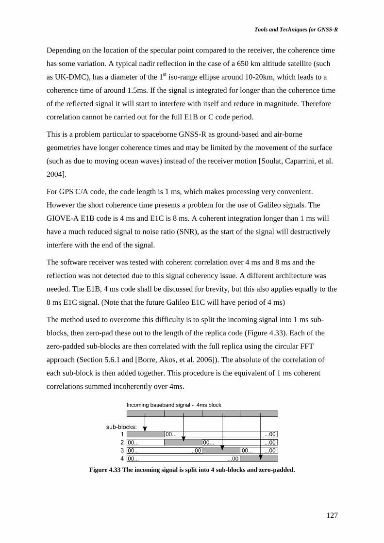
Tools and Techniques for GNSS-R
127
Depending on the location of the specular point compared to the receiver, the coherence time
has some variation. A typical nadir reflection in the case of a 650 km altitude satellite (such
as UK-DMC), has a diameter of the 1st iso-range ellipse around 10-20km, which leads to a
coherence time of around 1.5ms. If the signal is integrated for longer than the coherence time
of the reflected signal it will start to interfere with itself and reduce in magnitude. Therefore
correlation cannot be carried out for the full E1B or C code period.
This is a problem particular to spaceborne GNSS-R as ground-based and air-borne
geometries have longer coherence times and may be limited by the movement of the surface
(such as due to moving ocean waves) instead of the receiver motion [Soulat, Caparrini, et al.
2004].
For GPS C/A code, the code length is 1 ms, which makes processing very convenient.
However the short coherence time presents a problem for the use of Galileo signals. The
GIOVE-A E1B code is 4 ms and E1C is 8 ms. A coherent integration longer than 1 ms will
have a much reduced signal to noise ratio (SNR), as the start of the signal will destructively
interfere with the end of the signal.
The software receiver was tested with coherent correlation over 4 ms and 8 ms and the
reflection was not detected due to this signal coherency issue. A different architecture was
needed. The E1B, 4 ms code shall be discussed for brevity, but this also applies equally to the
8 ms E1C signal. (Note that the future Galileo E1C will have period of 4 ms)
The method used to overcome this difficulty is to split the incoming signal into 1 ms sub-
blocks, then zero-pad these out to the length of the replica code (Figure 4.33). Each of the
zero-padded sub-blocks are then correlated with the full replica using the circular FFT
approach (Section 5.6.1 and [Borre, Akos, et al. 2006]). The absolute of the correlation of
each sub-block is then added together. This procedure is the equivalent of 1 ms coherent
correlations summed incoherently over 4ms.
Figure 4.33 The incoming signal is split into 4 sub-blocks and zero-padded.

128
For a direct signal, this technique reduces the SNR in comparison to the straight forward 4 ms
coherent correlation, due to the squaring loss as the absolute of each sub-block is added
together. For a reflected signal the SNR improves significantly, as the coherent correlation is
kept inside the signal coherence time.
This method increases the processing load over that of GPS delay-Doppler map generation,
as for each 1 ms of input samples, a 4 ms long section of signal must be correlated. The FFT
length could be reduced if there is some a-priori knowledge of the code phase.
4.5.4. Experimental Verification
As well as verification of the concept on simulated signals, the receiver architecture was
demonstrated on real signals from space by collecting data from the UK-DMC GNSS-R
experiment. (See Section 2.4).
The UK-DMC receiver was designed for reception of just the GPS C/A signal at L1 which
have a null-to-null bandwidth of 2 MHz. For this experimental campaign it was necessary to
judge whether the available UK-DMC hardware was capable of receiving the wider
bandwidth GIOVE-A signals. In the experiments here, the receiver is not capable of
distortion-free digital sampling of the wider bandwidth Galileo E1 signal, due to insufficient
sampling rate and a narrow bandwidth IF filter.
The narrowest bandwidth part of the UK-DMC receiver is a SAW filter in the intermediate
frequency (IF) stage. The bandwidth of this part was measured from the flight model before
the satellite’s launch so the effect of the filter can be assessed now in simulation.
A BOC(1,1) signal was passed through a digital filter designed to have the same frequency
response as the SAW filter, Figure 4.34. The receiver bandwidth is smaller than the first lobe
of the signal. The filter has pass band of –5 dB at a width of 2.5 MHz. This acts to smooth
and reduce the peak of the correlation function as shown in Figure 4.35. Reading off from
this, the IF filter distorts the correlation shape reducing the peak correlation power by
20 log10(0.79) = 2.0 dB.
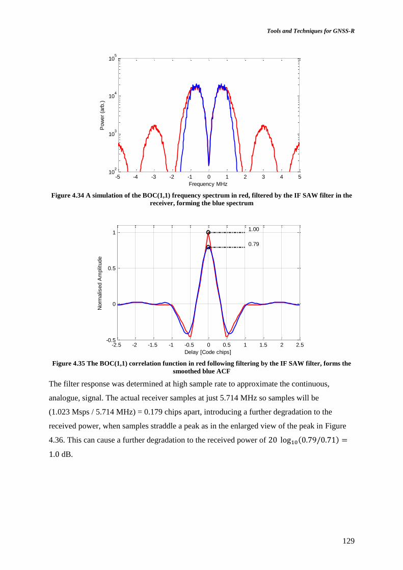
Tools and Techniques for GNSS-R
129
Figure 4.34 A simulation of the BOC(1,1) frequency spectrum in red, filtered by the IF SAW filter in the
receiver, forming the blue spectrum
Figure 4.35 The BOC(1,1) correlation function in red following filtering by the IF SAW filter, forms the
smoothed blue ACF
The filter response was determined at high sample rate to approximate the continuous,
analogue, signal. The actual receiver samples at just 5.714 MHz so samples will be
(1.023 Msps / 5.714 MHz) = 0.179 chips apart, introducing a further degradation to the
received power, when samples straddle a peak as in the enlarged view of the peak in Figure
4.36. This can cause a further degradation to the received power of 20 log10(0.79/0.71) =
1.0 dB.
-5 -4 -3 -2 -1 0 1 2 3 4 510
2
103
104
105
Frequency MHz
Pow
er
(arb
.)
-2.5 -2 -1.5 -1 -0.5 0 0.5 1 1.5 2 2.5-0.5
0
0.5
1
Norm
alis
ed A
mplit
ude
Delay [Code chips]
1.00
0.79
-5 -4 -3 -2 -1 0 1 2 3 4 510
2
103
104
105
Frequency MHz
Pow
er
(arb
.)
-2.5 -2 -1.5 -1 -0.5 0 0.5 1 1.5 2 2.5-0.5
0
0.5
1
Norm
alis
ed A
mplit
ude
Delay [Code chips]
1.00
0.79

130
Figure 4.36 Enlarged view of the filtered BOC(1,1) ACF
The conclusion is that Galileo signals should be detectable, but attenuated with the UK-DMC
receiver. It was considered that it was worthwhile trying to detect a reflection so a collection
was scheduled for a time when GIOVE-A passed over UK-DMC in such a way that the
specular reflection would fall within the nadir antenna beamwidth. The GNSS-R experiment
on UK-DMC has not been routinely targeted at these reflections; however one of these
opportunities was scheduled over for the 4th
November 2007 over the Arafua Sea, North of
Australia. The experiment recorded data for 20 seconds, the geometry was such that two
additional GPS specular reflections were recorded in the field of the receiving antenna,
Figure 4.37.
Figure 4.37 The geometry of UK-DMC and its receiver antenna pattern in red durign the Arafua sea data
collection.
-5 -4 -3 -2 -1 0 1 2 3 4 510
2
103
104
105
Frequency MHz
Pow
er
(arb
.)
-1 -0.8 -0.6 -0.4 -0.2 0 0.2 0.4 0.6 0.8 10.5
0.6
0.7
0.8
0.9
1
1.1
Norm
alis
ed A
mplit
ude
Delay [Code chips]
0.79
0.71
0.179 chips

Tools and Techniques for GNSS-R
131
For the data collection the Arafura Sea was predicted to be relatively calm. The European
Centre for Medium-Range Weather Forecasts, (ECMWF) model for the time predicted wind
speeds of ~15 km/h [ECMWF 2007]. This is a relatively smooth ocean surface, so a
relatively strong reflected signal would be expected.
Despite the difficulties due to the receiver distortions the direct E1B and E1C signals were
tracked to recover data bits and secondary code. Tracking was performed using the Dual-
Estimator tracking loop technique [Hodgart & Blunt 2007] and the prompt E1B and E1C
correlations were read out to measure 𝑑(𝑡) and 𝑐𝑠(𝑡).
Due to the receiver distortions, some effort was put into verifying the data was accurate. The
validity of the E1C secondary code retrieval can be determined by checking the secondary
code is the same as specified in the signal definitions. The detected phase of the E1C signal
has been correlated with the specification code [Galileo Project Office 2007]. The results of
which are shown in Figure 4.38. The secondary code has length 25 chips and repeats every
200 ms, so the correlation of magnitude 25 and repetition 200 ms indicates that the E1C
secondary code was received with no errors.
Figure 4.38 The received secondary code, correlated with the published code
It is considerably more complicated to check the validity of the E1B data retrieval, as it
requires implementation of the Viterbi decoder algorithm. As the data decoding is not
necessary for this test, the data retrieval can instead be checked using the 10 bit SYNC word,
which repeats at exactly 1 second intervals. This was verified to exist every second, or 250
symbols as seen in Figure 4.39. The cross-correlation is noisy as the SYNC word is only 10
bits long and can occur anywhere in the data. The SYNC word was found without error
(correlation magnitude being 10) at 1 second intervals throughout the data, so there is a high
confidence in the correct retrieval of E1B data bits.

132
Figure 4.39 E1B data, d(t), correlated with the 10 bit SYNC word and circled at 1 second intervals
The data and secondary code having been recovered from the direct signal were then
combined to process the reflected signal to map out the DDM. The coherent E1B + E1C
receiver architecture from Figure 4.29 was used.
An ocean reflected signal was successfully detected despite the signal power being less than
that from typical GPS reflections and the RF front end bandwidth significantly degrading the
signal. The reflection DDM has been plotted in Figure 4.40 and Figure 4.41. These used the
sub-block processing architecture to integrate for 1 ms coherently, then combined for
1 second (Figure 4.40) or 8 seconds (Figure 4.41) of incoherent accumulation. The DDM
colour scale is based on the signal power detectability measure Γ0 defined in Section 2.3.4.
Figure 4.40 DDM and delay map of the ocean reflected signal from GIOVE-A, 1 second integration.
Arafura Sea 04/11/2007
0 500 1000 1500 2000 2500 3000 3500 4000 4500-10
-5
0
5
10
15
Time in bit data-bit periods Td
Corr
ela
tion o
f re
ceiv
ed
data
with S
YN
C w
ord
corr( d(t), SYNC )
Marker for 250 symbols
Dela
y [
Code C
hip
s]
Doppler Hz
RGIOVEA-Nadir
-4000 -3000 -2000 -1000 0 1000 2000 3000 4000
0
5
10
15
20
25
30
35
Sta
ndard
devia
tions f
rom
mean
-2
-1
0
1
2
3
4
5
6

Tools and Techniques for GNSS-R
133
Figure 4.41 DDM and delay map of the ocean reflected signal from GIOVE-A, 8 second integration.
Arafura Sea 04/11/2007
The correlation power delay maps, on the right hand side, were produced from a cut through
the DDM at the central Doppler frequency.
The previously discussed receiver approaches were assessed for the received signal. The
coherent combination of L1B and L1C provided the greatest SNR. The UK-DMC
experimental receiver has an unmonitored automatic gain control making it impossible to
determine a radiometric measurement of signal power, although it is possible to make some
comparisons with the SNR of the received GPS signals and the transmission powers. The
signal to noise ratio for the GIOVE-A correlation power DDM is within the range of that seen
for GPS transmitters, which can be seen in the detectability metric explored for the UK-DMC
data collections in Section 3.2.
GPS and Galileo set a guaranteed minimum power for an ideally matched RHCP 0 dBi
polarised user receiver [Galileo Project Office 2007; GPS Directorate 2011] (usually defined
for the transmitter elevation angle higher than 10 degrees from the horizon). For the GPS C/A
code this is -158.5 dBW, although generally the received power levels of the GPS satellites
are between 1 and 5dB greater than the specified minimum power levels [Kaplan 2006]. The
minimum receiver power for a user on the ground for the GIOVE-A E1 band has been
measured as -155.5 dBW [Rooney, Unwin, et al. 2007]. This is split between the three
channels 22% to E1B and 22% to E1C and 44% to E1A. Basic comparing the power level is
carried out in Table 4.3
Dela
y [
Code C
hip
s]
Doppler Hz
RGIOVEA-Nadir
-4000 -2000 0 2000 4000
0
5
10
15
20
25
30
35
Sta
ndard
devia
tions f
rom
mean
-2
0
2
4
6
8
10
12
14
16

134
Table 4.3 GPS and GIOVE-A minimum received power comparison
GPS L1 C/A GIOVE-A:
−158.5 dBW
Separate E1B or E1C components:
22% of -155.5 dBW (or −6.6 dB) = −162 dBW each
Combining E1B an E1C coherently
−162 dBW + 3 dB resulting in−159.1 dBW
Combining E1B and E1C for GIOVE-A would result in an estimated power just 0.6 dB lower
than GPS C/A code power.
4.5.5. Discussion
In this section a signal processing architecture has been developed for optimal processing of
the open-service Galileo E1 signals by combining the sub-signals and processing in such a
way as to match the coherence time of the reflections. From this the first Galileo-type signal
reflection has been detected from orbit.
In addition to the post-processing demonstration, the approach for a practical real-time
architecture has been developed that will allow, future GNSS-R missions to target Galileo
reflections and therefore potentially double the coverage over that of using solely GPS
signals.
For the small satellite approach to GNSS-Reflectometry with a fixed gain antenna there is a
trade-off between antenna gain and sensing coverage, this is discussed in Section 3.6.
Increased SNR could be obtained through a higher-gain antenna, with corresponding smaller
ocean sampling area, or from optimising the receiver and processing techniques. This work
has maximised the received SNR without compromising the coverage.
The work here also presents an opportunity for further study into the advantages of the BOC
modulation in GNSS-R. The wider bandwidth can result in increased ground resolution, but
the large side-lobes in the auto-correlation function would usually be considered a
disadvantage for a radar waveform. A deconvolution approach may need to be used to realise
the advantages of the increased bandwidth.

Tools and Techniques for GNSS-R
135
The wider bandwidth pushed at the limits of the UK-DMC receiver, but the sampled RF
bandwidth can be improved on a new instrument so the results would be at least as good as
presented here. This will become increasingly relevant as the modernised GPS service is
additionally planning on implementing a BOC modulated civil service called L1C.
4.6. Stare Processing
The following section investigates a technique which is closer in concept to the traditional
ocean wind radar scatterometers, such as SeaWinds on the QuikScat satellite and is closely
coupled to that presented in [Jales 2010]. The surface measurement scheme is analysed with a
scattering model and on real data from orbit. It is shown to be a promising approach for
determining the surface roughness from GNSS-R. The impact of this processing scheme on
the instrument and the satellite platform are examined. In addition the receiver developments
required for real-time in-orbit operation, such as geometric tracking are verified on data from
the UK-DMC GNSS-R experiment and results compared to the model.
Stare processing is closely related to a technique originally proposed by Starlab, Barcelona,
which they refer to as SHARP processing. The SHARP approach is mentioned in [Germain
& Ruffini 2002] and the patent [Caparrini, Germain, et al. 2003], although there is little
published analysis and covers additional approaches for combining multiple receivers which
are not considered here. This interpretation of the technique, Stare Processing is based on
processing the reflected signal such that a fixed point on the ocean is measured multiple times
as the receiver moves over the surface. This is different conceptually from the DDM, which
maps the reflected signal's distortion in signal space.
Stare processing relates the reflected signal power back to the scattering point on the ocean
surface and the scattering geometry. This is closer to the operation of a traditional ocean wind
monostatic scatterometer, which measures the radar scattering cross-section at several
incidence angles, then retrieves the wind direction and speed from the inversion of a semi-
empirical model[Stewart 1985, chap.12.3]. Similarly Stare Processing extracts the bistatic
radar scattering cross-section for a range of incidence angles offering potential for a semi-
empirical model inverting measurements to determine a measure of surface roughness. This
mapping of the surface to the scattering geometry is also similar to the work in [Cardellach &
Rius 2007].
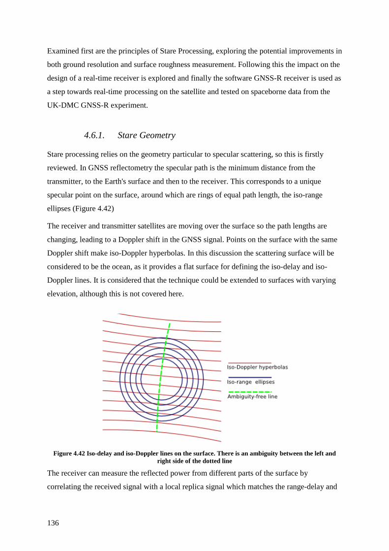
136
Examined first are the principles of Stare Processing, exploring the potential improvements in
both ground resolution and surface roughness measurement. Following this the impact on the
design of a real-time receiver is explored and finally the software GNSS-R receiver is used as
a step towards real-time processing on the satellite and tested on spaceborne data from the
UK-DMC GNSS-R experiment.
4.6.1. Stare Geometry
Stare processing relies on the geometry particular to specular scattering, so this is firstly
reviewed. In GNSS reflectometry the specular path is the minimum distance from the
transmitter, to the Earth's surface and then to the receiver. This corresponds to a unique
specular point on the surface, around which are rings of equal path length, the iso-range
ellipses (Figure 4.42)
The receiver and transmitter satellites are moving over the surface so the path lengths are
changing, leading to a Doppler shift in the GNSS signal. Points on the surface with the same
Doppler shift make iso-Doppler hyperbolas. In this discussion the scattering surface will be
considered to be the ocean, as it provides a flat surface for defining the iso-delay and iso-
Doppler lines. It is considered that the technique could be extended to surfaces with varying
elevation, although this is not covered here.
Figure 4.42 Iso-delay and iso-Doppler lines on the surface. There is an ambiguity between the left and
right side of the dotted line
The receiver can measure the reflected power from different parts of the surface by
correlating the received signal with a local replica signal which matches the range-delay and

Tools and Techniques for GNSS-R
137
Doppler shift of the chosen point. One of the difficulties in sensing around the specular point
is that there is an ambiguity in the signal coming from the ocean, as each iso-Doppler line
intersects the iso-range line in two places. However, there is a line through the specular point
which is ambiguity-free, (Figure 4.42). Using measurements only from this line allows
measurement of the reflectivity of a unique part of the surface, uncorrupted by additional
reflections. Choosing to measure from just this part of the scattering zone improves the
surface resolution, but ignores the ambiguous areas which may still provide valuable surface
measurement.
We are initially considering the case when the specular point moves along the ambiguity-free
line. This is clearly a special case, later this is extended away to more typical reflection
tracks. This is the case when the receiving satellite has a velocity aligned in the plane of the
transmitter, specular point and receiver (𝑻𝑺𝑹⃗⃗ ⃗⃗ ⃗⃗ ⃗⃗ plane) and passes directly over the specular
point. In this circumstance the ambiguity free line is aligned with the path of the specular
point, in which case multiple reflectance measurements are possible, over time, for one point
of the ocean, each with a different scattering angle. This is similar to the monostatic
scatterometers that already routinely retrieve ocean wind observations by inversion of the
measured reflectance at three different scattering angles [Stewart 1985]. The reflectance in
radar terminology is known as the scattering cross-section or 𝜎0 and has been defined for
GNSS-R in Section 2.2.
In contrast, the DDM receiver approach ignores the movement of these iso-lines across the
surface, and instead accumulates the signal power for a fixed grid of delay and Doppler
offsets. Therefore each point on the DDM corresponds to the reflected power from sometimes
two separate points that move across the ocean surface during the integration time.
The special case geometry is shown in Figure 4.43, with a planar surface for ease of
understanding. The transmitter, 𝑻, is drawn to be much further from the surface than the
receiver. As the receiver, 𝑹, moves, the specular point moves with it. A stare point 𝑷 is
chosen such that the specular point passes through it. As the receiver moves, the processing is
set up to stare at 𝑷, so it is able to measure the reflected power from 𝑷 at a range of bistatic
angles, 𝛽. Choice of point 𝑷 is restricted to be within a certain distance of the specular point
by the RF link budget (and constrained to be within the receiver’s antenna footprint).

138
Figure 4.43 GNSS-R Stare processing geometry at three different times. Left diagram earliest in time and
right diagram being latest.
To demonstrate the association of the stare point delay and Doppler with the DDM, an
example DDM was chosen from the UK-DMC data collections and is shown in Figure 4.44.
A point 𝑷 was chosen to coincide with the specular point at 8 seconds progression through
the 16 second data-set (the length being restricted by the data recorded by UK-DMC). The
stare point delay and Doppler of 𝑷 is plotted as a circle on the DDM every 400 ms for the
period 8 seconds before and 8 seconds after the time when 𝑺 = 𝑷. (The DDM corresponds to
the 1 second integration centred on 𝑺 = 𝑷.) The Stare processing approach can be seen to
select only part of the DDM, but these correspond to the greatest reflected signal power.
Figure 4.44 DDM with stare point delay and Doppler plotted. (R12 dataset, PRN15)
The objective is to determine surface roughness, the way in which Stare processing can
achieve this is by measuring how the scattering cross-section (𝜎0) changes with scattering
angle, whilst the receiver stares at the fixed point on the surface.

Tools and Techniques for GNSS-R
139
4.6.2. Scattering Cross Section
To understand measurement of the scattering cross-section in the case of Stare processing we
can use the bistatic radar equation, Equation (2.1). The model of the received power is
formed from the integral over all possible scattering targets with the region reduced to the
convergence of the zones selected by the receiver antenna pattern, the scattering zone, and the
alignment of the receiver selected delay and the Doppler.
An infinitesimal point on the ocean cannot be selected for point 𝑷 as the signal has finite
bandwidth causing a limited resolution in delay determination. In addition there is a limited
resolution to the Doppler frequency determination due to the limited coherent integration
time. These terms result in the signal ambiguity function (AF) as shown in Figure 2.6 for
GPS L1 C/A used throughout this section. The work would apply to other GNSS signals with
appropriate modification to the AF.
During a Stare processing observation the area of the surface selected by the AF will change
as the satellites move. This area can be modelled by projecting the idealised AF onto the
surface as in Figure 4.45 (Column A). Despite the similar appearance to a DDM, these are
plots not of signal space, but a plan view of the ocean surface. The iso-Doppler (red), iso-
delay (blue) and ambiguity-free (green) lines are shown in Figure 4.45 (Column B). The time
series presents part of a Stare processing observation with point 𝑷 fixed to location (0,0). The
receiver starts directly below the transmitter and as it moves leftwards, the specular point also
moves from (0,0) to the left. The time series is plotted at 4 second intervals.
As the receiver moves, it provides measurements of a fixed point on the ocean through
steering the correlators to the delay and Doppler curve. The stare point remains fixed, but due
to the changing geometry the angle the shape and area of the selected area changes. The AF
can be seen as projected on to the surface. The side-lobes of the sinc-shaped Doppler
dimension are visible. This causes some along-track cross-talk and may limit the applicability
of the method to the open ocean as the littoral environment may add significant reflections in
the side-lobes.
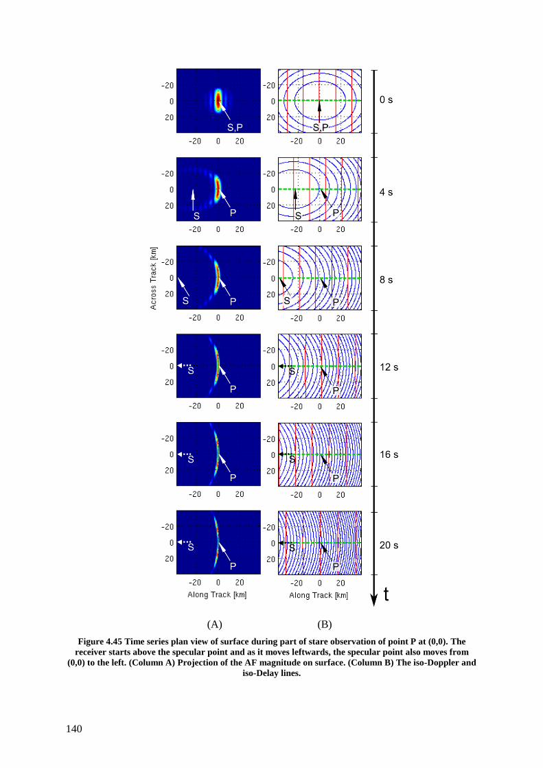
140
(A) (B)
Figure 4.45 Time series plan view of surface during part of stare observation of point P at (0,0). The
receiver starts above the specular point and as it moves leftwards, the specular point also moves from
(0,0) to the left. (Column A) Projection of the AF magnitude on surface. (Column B) The iso-Doppler and
iso-Delay lines.

Tools and Techniques for GNSS-R
141
4.6.3. Theoretical Model
To understand the sensitivity of Stare processing to the surface roughness a model of the
scattering is needed. The Z-V model as introduced in Section 2.2.3 will now be applied to the
Stare processing scenario to gain insight into its sensitivity to surface roughness. The
limitations of the model have been discussed previously with reference to some
improvements, but despite this the Z-V model has become a commonly used model in GNSS-
R due to its relative simplicity.
The Z-V model, bistatic radar equation can be used to separate the influences of the varying
geometry from the measurement of the scattering cross-section. The bistatic radar equation
predicts the received power as an integral over the surface, 𝝆, where the signal correlation
results in a non-zero ambiguity function. We can assume that over the small area selected by
the AF that several of the terms are constant. The modelled expectation of the received power
⟨𝑃𝑅𝑥𝑅 ⟩, then depends on the transmitted power 𝑃𝑇𝑥; the transmitter antenna gain to the stare
point, 𝐺𝑇𝑥(𝑷), receiver antenna gain in direction of the stare point, 𝐺𝑅𝑥𝑅 (𝑷) and the path
lengths from the stare point to receiver and stare point to transmitter, |𝑹𝑷⃗⃗ ⃗⃗ ⃗⃗ ⃗|, |𝑻𝑷⃗⃗ ⃗⃗ ⃗⃗ ⃗| respectively.
The scattering cross-section of the surface is also assumed constant over this small area. This
allows the simplification of using the terms integrated over the scattering area, 𝐺𝑇𝑥, 𝜎0, etc.
(without 𝝆 dependence). So repeating the bistatic radar equation but now for the return when
the correlator is matched to the delay and Doppler of the stare point 𝑷,
⟨𝑃𝑅𝑥
𝑅 ⟩ = Tcoh2 λ2 ∙ 𝑃𝑇𝑥 ⋅ 𝐺𝑇𝑥(𝑷) ∙ 𝐺𝑅𝑥
𝑅 (𝑷) ⋅ 𝜎0(𝑷)
(4π)3 ⋅ |𝑹𝑷⃗⃗⃗⃗⃗⃗ |2∙ |𝑻𝑷⃗⃗ ⃗⃗ ⃗|
𝟐∬𝜒2(𝑡 − 𝑡′(𝝆), 𝑓 − 𝑓′(𝝆))d2𝝆
𝝆
(4.32)
The surface corresponding to that selected by the ambiguity function 𝜒, is separated into an
area, 𝐴, through the integral over the surface,
𝐴 = ∬𝜒2(𝑡 − 𝑡′(𝑷), 𝑓 − 𝑓′(𝑷)) d2𝝆
𝝆
(4.33)
To determine the radar scattering cross-section the integrated bistatic radar equation can be
rearranged to,
𝜎0(𝑷) =(4𝜋)3 ∙ ⟨𝑃𝑅𝑥
𝑅 ⟩ ∙ |𝑹𝑷⃗⃗⃗⃗⃗⃗ |2∙ |𝑻𝑷⃗⃗ ⃗⃗ ⃗|
2
Tcoh2 ⋅ 𝜆2 ∙ 𝑃𝑇𝑥 ∙ 𝐺𝑇𝑥 ∙ 𝐺𝑅𝑥
𝑅 ∙ 𝐴 (4.34)

142
This shows that to measure 𝜎0 the ratio of transmitted to received power must be measured,
𝑃𝑅𝑥𝑅 𝑃𝑇𝑥⁄ . However the measurement is also affected by the geometrical factors which are the
ranges the antenna gains 𝐺𝑇𝑥, 𝐺𝑇𝑥𝑅 , and the AF surface area selected, 𝐴. Absolute radiometric
power measurement of 𝑃𝑇𝑥 and 𝑃𝑅𝑥𝑅 are therefore not needed to determine absolute 𝜎0, but
accurate measurement of the power ratios is needed.
In Stare processing, the value of 𝜎0 is mapped out over the range of incidence angles. By
inspecting the scattering term in Equation (2.17), it can be seen that the value of the slope
PDF could in principle be mapped out without reliance on a model for the surface slopes. The
approach here is instead to apply a model of the surface to an example Stare processing
geometry for a range of ocean roughness conditions to determine the expected sensitivity to
the surface.
For this the ocean surface model of [Elfouhaily, Chapron, et al. 1997], from Section 2.2.4 is
used. This was shown to predict a well-developed smooth ocean of 𝑈10 wind speed 1 m/s to
have mss = 0.0005; a rough sea with 𝑈10 wind speed of 25 m/s results in a mss of 0.016. An
omni-directional mss was used, as Stare processing would be measuring the mss in the 𝑻𝑺𝑹⃗⃗ ⃗⃗ ⃗⃗ ⃗⃗
plane and the measurement of the wave direction is not applied within the scheme.
As the Stare processing concept is measuring the angular distribution of 𝜎0, this is effectively
measuring the size of the scattering zone, which in turn is related to the roughness. The
sensitivity to the roughness through the extent of the scattering zone can be seen in the
modelled response in Figure 4.46. This models a Stare observation where 𝑷 and 𝑺 are chosen
to coincide at 8 seconds.

Tools and Techniques for GNSS-R
143
(A) (B)
Figure 4.46 Model of the scattering cross-section profile during a Stare processing measurement for a
range of ocean conditions. (A) shows the absolute 𝝈0 (B) shows the normalised 𝝈0.
It can be seen that for calm ocean surfaces the cross section profile is a narrower shape, while
for rougher surfaces the profile is flatter. Hence a measure of mss can be taken from the
profile.
The change in profile with mss in Figure 4.46 (B) indicates that absolute calibration of the
received power ratio is not essential as there is still sensitivity to surface roughness with a
normalised scattering cross-section. This is defined as,
normalised 𝜎0 =𝜎0
𝜎0|𝑺=𝑷
(4.35)
The absolute measurement of 𝜎0 is modelled in Figure 4.46 (A) and then normalised 𝜎0 in
Figure 4.46 (B).
From these two graphs it can be seen that the surface roughness sensitivity is in both the
amplitude and the width of the 𝜎0–time profile. The rougher the surface the greater is the
extent of the scattering zone and so the reflection power is reduced and spread out across the
time period of the stare observation.
When using normalised 𝜎0, Figure 4.46 (B), the part of the curve with the greatest SNR
(when 𝐒 = 𝐏) has no sensitivity to surface roughness due to our definition in Equation (4.35).
This shows that by using relative calibration of direct and reflected power (to form Figure
2 4 6 8 10 12 14 16
20
40
60
80
100
120
140
160
180
200
Time [s]
0
0 model for point P with time
mss = 0.0005
mss = 0.0010
mss = 0.0020
mss = 0.0040
mss = 0.0060
mss = 0.0080
mss = 0.0100
mss = 0.0120
mss = 0.0140
mss = 0.0160
2 4 6 8 10 12 14 16
0.3
0.4
0.5
0.6
0.7
0.8
0.9
1
Time [s]
Norm
alis
ed
0
Normalised 0 model for point P with time
mss = 0.0005 mss = 0.0010 mss = 0.0020 mss = 0.0040 mss = 0.0060 mss = 0.0080 mss = 0.0100 mss = 0.0120 mss = 0.0140 mss = 0.0160

144
4.46 (A)) then the expected sensitivity to the surface roughness would be improved.
Additionally it can be seen from the model that the sensitivity of 𝜎0 to the surface mss
decreases for the rougher conditions.
Whether the calibration is needed depends on whether there is sufficient sensitivity to surface
roughness for a specific GNSS-R application. Whilst the method for retrieving a physical
measurement, such as ocean mss, is being developed and validated, the question of whether
there is a requirement for absolute or normalised 𝜎0 is undecided. A calibration approach for
the power ratios is presented later as GNSS-R can use a simpler method than needed by
radiometer instruments. It is important to note that under the proposed scheme, information
on surface roughness should be evident from the width of the normalised 𝜎0 vs. time curve
(as in Figure 4.46 (B)), this means that absolute 𝜎0, would not be required, which would
relax the requirement for calibration of the measured signal power.
The Stare processing technique relies on the radar equation, which is based on the assumption
of returns from a very large number of independent scatterers [Zavorotny & Voronovich
2000]. The scattering surface meets this assumption of the radar equation if the surface is
sufficiently rough. The Rayleigh criterion in Section 2.2.3 showed that this is the case for
reflections away from the Earth’s limb. For the more glancing reflections, the Stare
processing approach would need modifications to the modelled radar equation.
To retrieve a measure of roughness from the 𝜎0 measurements, it is likely that a semi-
empirical model will need to be developed using a combination of models and satellite
measurements tied-up with in-situ data. This has been the case with the existing monostatic
ocean scatterometers [Liu 2002]. It is anticipated that a significant amount of data would
need to be collected as each measurement has a different scattering geometry, an issue that is
less of a problem with the monostatic scatterometers.
4.6.4. The Area Term
To be able to determine either 𝜎0 or normalised 𝜎0, the area that is selected on the ocean
needs to be determined as this changes during the stare observation. This will depend on the
geometry of receiver, transmitter and the Earth's surface, as well as the modulation and
bandwidth of the GNSS signal. The integral in Equation (4.33) needs to be evaluated for each
measurement in the stare observation.

Tools and Techniques for GNSS-R
145
To perform the area calculation, the integration that is implemented uses a spherical Earth, so
that, 𝝆, is constrained to the sphere's surface, although this could later be extended to an
ellipsoidal or undulating model. Taking the approach in [Zavorotny & Voronovich 2000], a
BPSK GNSS signal can be approximated by two independent functions of delay and
frequency offset. The area of the ambiguity function projected onto the ocean surface is
calculated numerically from Equation (4.33).
There is no requirement for real-time calculation of the area correction on the satellite. It can
be applied as a post processing step on the ground as long as the receiver, transmitter, and
stare point positions and velocities are recorded.
The area integral has been calculated to show the trend of area with distance from the
specular point. An example of this where the receiver is directly below the transmitter (𝜃 =
0) is shown in Figure 4.47. The lower figures show the plan view of the Earth’s surface with
the surface colour corresponding to the AF, 𝜒.
Figure 4.47 (Above) Area integral, A, with distance of Stare point from specular point. (Below Left) Plan
view of the selected surface for |P-S| = 0 km and (Below Right) |P-S| = 115 km. Where P is at (0,0).
0 20 40 60 80 100 12040
50
60
70
80
90
100
Distance of Stare point from Specular point [km]
AF
are
a [
km
2]
Area of ocean illuminated by AF
Along Track [km]
Acro
ss T
rack [
km
]
-50 0 50
-50
0
50
Along Track [km]
Acro
ss T
rack [
km
]
-50 0 50
-50
0
50
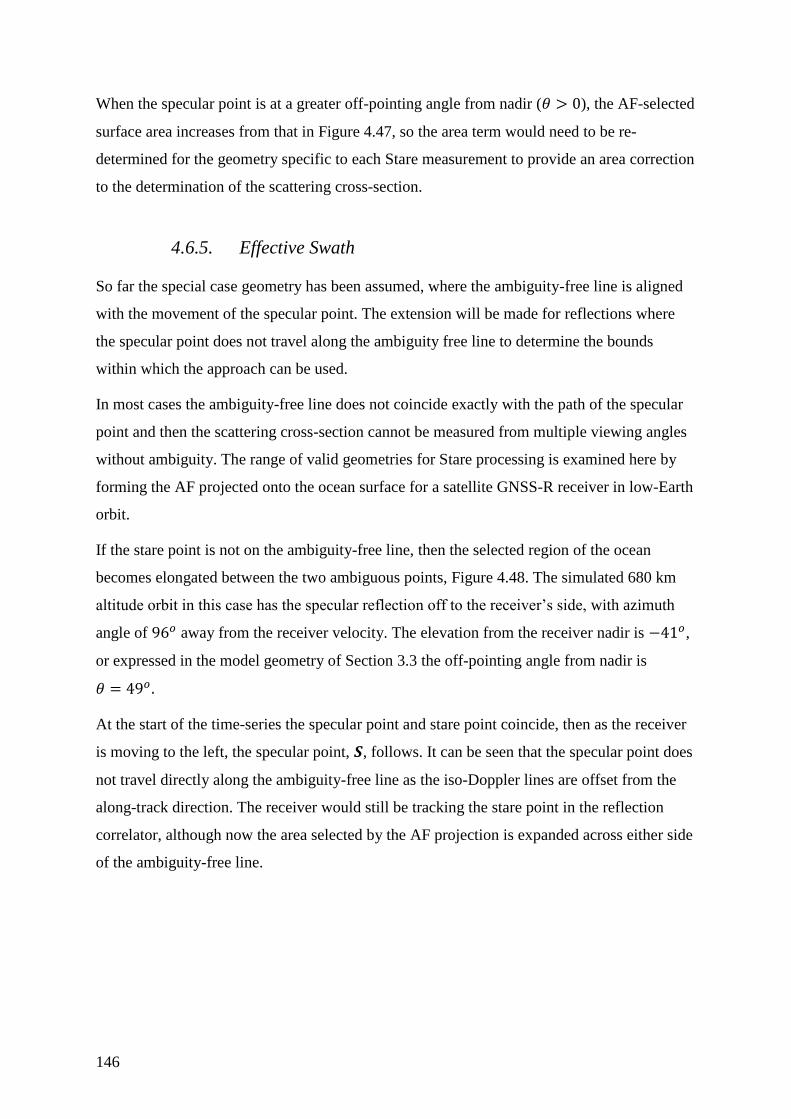
146
When the specular point is at a greater off-pointing angle from nadir (𝜃 > 0), the AF-selected
surface area increases from that in Figure 4.47, so the area term would need to be re-
determined for the geometry specific to each Stare measurement to provide an area correction
to the determination of the scattering cross-section.
4.6.5. Effective Swath
So far the special case geometry has been assumed, where the ambiguity-free line is aligned
with the movement of the specular point. The extension will be made for reflections where
the specular point does not travel along the ambiguity free line to determine the bounds
within which the approach can be used.
In most cases the ambiguity-free line does not coincide exactly with the path of the specular
point and then the scattering cross-section cannot be measured from multiple viewing angles
without ambiguity. The range of valid geometries for Stare processing is examined here by
forming the AF projected onto the ocean surface for a satellite GNSS-R receiver in low-Earth
orbit.
If the stare point is not on the ambiguity-free line, then the selected region of the ocean
becomes elongated between the two ambiguous points, Figure 4.48. The simulated 680 km
altitude orbit in this case has the specular reflection off to the receiver’s side, with azimuth
angle of 96𝑜 away from the receiver velocity. The elevation from the receiver nadir is −41𝑜,
or expressed in the model geometry of Section 3.3 the off-pointing angle from nadir is
𝜃 = 49𝑜 .
At the start of the time-series the specular point and stare point coincide, then as the receiver
is moving to the left, the specular point, 𝑺, follows. It can be seen that the specular point does
not travel directly along the ambiguity-free line as the iso-Doppler lines are offset from the
along-track direction. The receiver would still be tracking the stare point in the reflection
correlator, although now the area selected by the AF projection is expanded across either side
of the ambiguity-free line.

Tools and Techniques for GNSS-R
147
(A) (B)
Figure 4.48 Time series plan view of surface, whilst staring at fixed point P at (0,0). Views at 4 second
intervals through simulated UK-DMC orbit. (Column A) Projection of the AF magnitude on surface.
(Column B) The iso-Doppler and iso-Delay lines
148
The case depicted in Figure 4.48 is typical in that the ambiguity free line is very closely
aligned with the path of the specular point. This is due to the Doppler frequency of the
reflection being dominated by the receiver velocity for a GNSS-R receiver in low-Earth orbit.
The spread of the AF from this skew of the ambiguity-free line results in a spread in the
measurement and a corresponding reduction in resolution. Whether the measurement
resolution is too poor to provide a useful observation will depend on whether the assumptions
used in the bistatic radar equation hold true; in particular, whether the scattering cross-section
is constant over the, AF selected, surface. If we make the estimate that the ocean surface
wind can be considered stationary over scales of up to 100 km, then we can set this as the
maximum allowable resolution cell, then the usable geometries for Stare processing can be
determined.
The surface resolution was investigated for Stare processing over the range of receiver and
transmitter geometries from a 700 km altitude receiver in a circular orbit. The stare point 𝑷 is
chosen so as to coincide with the specular point 𝑺, and the receiver orbit propagated back for
Δ𝑇 = 10 seconds to provide a representative observation period. The AF is then projected
onto the surface to determine the resolution.
With no loss of generality the receiver location 𝑹, is chosen to be on the z-axis, then the
geometry chosen by selecting the specular point location 𝑺 and from this the corresponding
transmitter position 𝑻. To enumerate the possible stare geometries the specular point was
parameterised by two angles: the off-pointing angle between receiver nadir and specular
point, 𝜃 and the azimuth angle 𝜙 of the specular point from the receiver velocity vector.
These are defined in Figure 4.49.

Tools and Techniques for GNSS-R
149
Figure 4.49 Geometry used to parameterise specular point location for investigation of Stare processing
resolution
To determine the transmitter position corresponding to the chosen specular point, the angular
difference, Θ, of the transmitter and receiver radials (as defined in Figure 3.4) was
determined using Equation (3.7). So that the transmitter position is,
𝑻 = (
𝐺 ⋅ cos Θ𝐺 ⋅ sin Θ ⋅ sin(𝜙)𝐺 ⋅ sin Θ ⋅ cos (𝜙)
) (4.36)
where 𝐺 is the orbital radius of the transmitter.
For propagating the circular orbit, the receiver’s velocity is around the x-axis, with angular
speed,
𝜔 = √𝐺𝑀/|𝑹|3 (4.37)
where 𝐺 is the gravitational constant and 𝑀 the mass of the Earth. The transmitter’s angular
velocity is only 13% of that of the receiver so is approximated as stationary, which allows the
geometry to be simplified to depend on only the specular point location defined by 𝜃 and 𝜙.
The receiver location after propagation, 𝑹′ is
𝑹′ = (
0𝐿 ⋅ sin (ω ⋅ Δ𝑇)𝐿 ⋅ cos(𝜔 ⋅ Δ𝑇)
) (4.38)

150
where 𝐿 is the orbital radius of the receiver. From this propagated receiver position and the
original transmitter position the specular point is chosen to be the stare point 𝑷.
The AF can now be projected onto the surface, for a stare point 𝑷, separated from the
specular point 𝑺 by its motion over time period Δ𝑇. Through following this approach, the AF
projected onto the surface can be parameterised to any specular point location relative to the
receiver’s position and velocity.
The area of the AF is calculated numerically from Equation (4.33) which is plotted in
Figure 4.50 (A) over a range of 𝜙 and 𝜃. For this 700 km altitude scenario 𝜃 > 64.3𝑜 is
above the horizon. The more glancing reflections have a greater surface area as the iso-
Doppler and delay regions expand. It was seen previously that the selected AF area tends to
elongate so the extent or width is a better measure for determining if the selected area will
meet the conditions. The width at half-maximum AF (𝜒2) is calculated numerically and
plotted over the range specular point locations in Figure 4.50 (B).
(A) (B)
Figure 4.50 Size of the signal AF projected onto the surface, for range of specular point locations.(A)
shows the selected surface area. (B) shows the half-power width of the AF.
The special case considered has azimuth (𝜙) at 0𝑜 or 180𝑜. It might be expected that specular
points passing either side of the receiver's ground track (𝜙 = ±90o azimuth) would suffer
from a resolution loss due to the ambiguity problem, however the specular point always
moves close to the ambiguity free line. The resolution limit only starts to become a problem
with the more glancing reflections, when the specular point is a large angle from nadir, above
around 𝜃 > 40𝑜. This is when the resolution starts to approach failing the requirement of
sensing the ocean within its stationarity of 100 km resolution.
Specular point azimuth () [Degrees]
Off
-poin
ting f
rom
receiv
er
nadir (
)
[D
egre
es]
0 50 100 150
0
5
10
15
20
25
30
35
40
AF
Surf
ace A
rea [
km
2]
80
100
120
140
160
180
Specular point azimuth () [Degrees]
Off
-poin
ting f
rom
receiv
er
nadir (
)
[D
egre
es]
0 50 100 150
0
5
10
15
20
25
30
35
40
AF
surf
ace e
xte
nt
[km
]30
35
40
45

Tools and Techniques for GNSS-R
151
The result of this is that under the simulated conditions the effective swath of a GNSS-R
sensor in Stare processing mode will be limited by the antenna beam-width rather than the
decrease in resolution from the ambiguity in reflected signals.
4.6.6. Impact On Receiver
One of the key advantages of the Stare processing technique is that a normalised 𝜎0
measurement (Equation 4.35) should be sufficient to retrieve information on the surface
roughness, as suggested by the modelling shown in Figure 4.46, obviating the need for
absolute radiometric calibration. The scattering cross-section is a measure of the ratio of
incident power to transmitted power, so there is no need to measure the absolute radiometric
power from either source. Calibration is discussed in Section 4.7, providing a possible
suitable solution using a cross-over switch.
The stare point, 𝑷, can be targeted in the receiver processing by choosing the corresponding
delay and Doppler shift. This geometric reflection tracking is the same open-loop approach
developed in Section 4.2, although instead of targeting the correlators at the calculated delay
and Doppler of the specular point, the stare point is chosen. The required delay and Doppler
for a stare point is shown in Figure 4.51, showing the difference between the 𝑻𝑺𝑹⃗⃗ ⃗⃗ ⃗⃗ ⃗⃗ and 𝑻𝑷𝑹⃗⃗⃗⃗ ⃗⃗ ⃗⃗ ⃗
paths. This example simulation assumes a UK-DMC-like circular orbit at 680 km altitude.
The receiver velocity is aligned with the 𝑻𝑺𝑹⃗⃗ ⃗⃗ ⃗⃗ ⃗⃗ plane and the 𝑺 and 𝑷 points coincide at 100 s.
Figure 4.51 Delay and Doppler difference between TSR and TPR paths over time. P=S at 100 seconds.

152
4.6.6.1. On-board Processing
The Stare processing technique reduces the data rate that needs to be transmitted to the
ground. If the GNSS-R instrument has a data rate of only a small fraction of the total satellite
downlink capacity then it would be an attractive secondary payload. The reduction in the data
rate is effectively due to only recording the correlation power along the ambiguity-free line,
and discarding the rest of the DDM. This waste can be justified on the basis of the ambiguity
either side of the line distorting measurement of the scattering cross-section.
The saving in data-capacity is substantial, as can be seen from a simple analysis of the
measurements along the track of a specular point, Figure 4.52. Each 𝜎0 measurement is over
the integration duration of the coherent and incoherent accumulations: (𝑇𝑐𝑜ℎ ∙ 𝑀) seconds.
The receiver stares for a total of t seconds at each stare point P0, P1 , P2 .…then the number of
integrations per surface point is 𝑁 = 𝑡/(𝑇𝑐𝑜ℎ 𝑀).
Figure 4.52 Stare processing surface measurements at surface points P0, P1, P2… Each ray corresponds to
a single 𝝈0 measurement for the corresponding Pi
The distance between stare points is chosen so that the surface resolution is d km along the
path of each specular point. The specular point velocity of 𝑣, will cause the receiver to pass
𝑣/𝑑 points per second. This results in a total number of measurements along the path
travelled by the specular point of 𝑁𝑀 𝑣/𝑑 per second.

Tools and Techniques for GNSS-R
153
Taking suitable numbers: 𝑀 = 500, 𝑇𝑐𝑜ℎ = 1 ms, 𝑡 = 20 s, 𝑣 = 6 km/s and a surface
resolution of 𝑑 = 10 km, then with the number of measurements per stare point will be,
𝑁 = 40 and 𝑁 𝑣/𝑑 = 24 simultaneous measurements per specular point per second.
Now to determine the total data rate, assume 𝑄𝑏 bit measurement quantisation, and operated
for 24 hours.
Data rate per channel = 60 ∙ 60 ∙ 24 ∙ 𝑄𝑏 ∙ 𝑁 ∙𝑣
𝑑 bits per day
(4.39)
With the numbers from the example scenario, this is just 10 Mb per reflection channel per
day. This compares very well to the approach of downlinking the raw data at 6000 Gb per
day (Section 5.2), or the full DDM at 16 Gb per reflection channel per day (Section 5.2.2)
4.6.6.2. Resolution
The resolution of Stare processing can be further analysed by comparing it to using the full
DDM for inversion to surface roughness. The current approaches to ocean roughness retrieval
from the DDM generally operate on the whole DDM. This corresponds to something around
25 code chips of delay from the specular point for spaceborne data with a UK-DMC-like
antenna and orbit. In Figure 4.53 an example DDM from a UK-DMC data set is plotted with
the corresponding surface iso-Doppler and iso-delay lines. If the whole DDM is used to
determine one ocean roughness measurement, then the resolution will be 200 km by 200 km
(for the best-case reflections near nadir).
Figure 4.53 Correspondence between surface and DDM areas
The Stare processing approach selects a single, high-resolution, cell that is repeatedly
measured as the receiver moves. The resolution advantage comes as this approach is

154
effectively selecting a single pixel from each of a series of DDMs (where the pixel selected
moves through the DDMs to always corresponds to the same surface point). The
improvement to the resolution can be seen by referring to Figure 4.54, where a series of stare
measurements have been carried out. A set of 10 Stare observations have independently
measured a patches on the surface, 𝑷𝒏. The resolution improvement can be further quantified
with the aid of Figure 4.50(B). It can be seen that the half-power width of the selected stare
point is 25 km for the near nadir-case. This compares very well to the whole-DDM method
that uses all the scattering from with a 200 km x 200 km area.
Figure 4.54 Ground resolution from Stare processing, showing 10 measurements
Additionally the Stare approach gives additional flexibility, as the surface patches 𝑷𝒏 are
independent then spatial averaging can be performed as a trade-off between surface
resolution and measurement variance.
4.6.7. Orbital Results
The Stare processing technique was tested on the limited dataset available from the UK-DMC
GPS-R experiment. Subsets of the data have been analysed using delay map and DDM based
analysis [Gleason & Adjrad 2005], [Clarizia, Gommenginger, et al. 2009]. This is the first
time that the data has been analysed by the Stare processing approach. In addition, previous
implementations of GNSS-R software receivers [Gleason 2006] had used a blind search for
the reflection before processing the DDM. This is the first implementation where the
reflections have been tracked in UK-DMC data from a geometric tracking of the predicted
delay and Doppler.
The structure of the software receiver was shown in Figure 4.1. From the zenith antenna raw
samples a position solution is obtained directly, so that geometric tracking can be used to
Tools and Techniques for GNSS-R
155
track the reflection in the nadir antenna. The data sets are limited each to 20 seconds of raw
samples by the storage space on the satellite. The software receiver uses the first few seconds
to initialise. This is from 2 to 6 seconds depending on the timing of the first data sub-frame,
so leaves 13 to 16 seconds remaining for GNSS-R measurements.
Specular point calculation took into account the WGS-84 ellipsoid with undulations. The
method was based on minimisation of the transmitter, Earth, receiver distance by constrained
optimisation using the projected sub-gradient method as discussed in Section 4.4.3, with the
addition of geoid WGS-84 undulations. The predicted time delay then includes the
atmospheric models that are standard to GNSS navigation receivers, Klobuchar model of the
ionosphere and the wet/dry component model of the neutral atmosphere [Kaplan 2006].
Stare processing relies on sub-chip accuracy of the reflection tracking to steer to the delay
and Doppler of a surface point. The accuracy of the software receiver’s open-loop, geometric
tracking was analysed in Section 4.4.6 and found to have mean delay error of −444.5 m with
standard deviation 664.9 m. To ensure that the Stare processing delay is aligned to sub code
chip accuracy with the reflected signal, the delay offset was measured from the DDM
processing and was applied for each data set, which effectively closes the tracking loop.
The UK-DMC receiver has no measures for calibration, and there is no control over the
Automatic Gain Control so we are limited to a normalised 𝜎0 measurement with this receiver.
A calculation of 𝜎0 was performed for stare points in all the UK-DMC data collections,
taking into account the change in radar equation parameters due to the changing geometry,
using Equation (4.34). Each of the terms of the radar equation vary through the observation
and are plotted individually in Figure 4.55 for an example data collection ‘R44’ for GPS C/A
code PRN 10. The specular point, at the start of this collection, is at 𝜙 = −177𝑜 azimuth and
𝜃 = 20𝑜 elevation from the receiver’s nadir.
Figure 4.55 (A) Shows the measured signal power from the correlator steered to the stare
point chosen to coincide with the specular point at 9 seconds into the data collection (half
way through the file following initialisation time). Figure 4.55 (B) shows the predicted area
of the AF on the surface, 𝐴. Figure 4.55 (C) shows the antenna gain in the direction of the
stare point. (D) Shows the combined range terms of the bistatic radar equation. (E) shows the
scattering cross-section 𝜎0 for a range of mss from the smoothest to roughest ocean
conditions and (F) the normalised 𝜎0.

156
(A) (B)
(C) (D)
(E) (F)
Figure 4.55 Stare processing measurement from a UK-DMC dataset taken over the ocean. Specular point
and stare point coincide at 9 seconds. (Dataset R44, PRN 10).
0 5 10 15 2070
80
90
100
110
120
130
Time [s]
AF
are
a [
km
2]
Area of ocean illuminated by AF
0 5 10 15 200
2
4
6
8
10
12
Time [s]
Ante
nna g
ain
[dB
i]
Antenna gain for point P during stare
0 5 10 15 20
262
263
264
265
Time [s]
10 *
log
10(
RR2 R
T2 )
Range terms of the Bistatic radar equation
2 4 6 8 10 12 14 16
20
40
60
80
100
120
140
160
180
200
Time [s]
0
0 model for point P with time
mss = 0.0005
mss = 0.0010
mss = 0.0020
mss = 0.0040
mss = 0.0060
mss = 0.0080
mss = 0.0100
mss = 0.0120
mss = 0.0140
mss = 0.0160
2 4 6 8 10 12 14 16
0.4
0.5
0.6
0.7
0.8
0.9
1
Time [s]
Norm
alis
ed
0
Normalised 0 model for point P with time
mss = 0.0005 mss = 0.0010 mss = 0.0020
mss = 0.0040 mss = 0.0060 mss = 0.0080
mss = 0.0100 mss = 0.0120 mss = 0.0140 mss = 0.0160

Tools and Techniques for GNSS-R
157
The parameter of interest is the scattering cross section, 𝜎0, as this is the term that has
sensitivity to surface roughness. There is a similar magnitude of variation across the
observation for 𝜎0 as there is for the area term or antenna gain. So it is particularly important
to provide good determination of the antenna gain and the modelled surface area.
Due to the limited duration of the real spaceborne data collections available, the Stare
processing observation is cut short to just 18 seconds in total. To allow observation of the tail
corresponding to large distance between 𝑺 and 𝑷, three stare points were selected at 54 km
steps. For each case, all the terms of the bistatic radar equation are combined to model the
predicted received reflection power. The measured signal power is plotted alongside the
modelled 𝑃𝑅𝑥𝑅 in the left column of Figure 4.56. The right column shows the corresponding
section of the delay Doppler map with a circle every 400 ms. The coherence time used for the
integration in this processing was, 𝑇𝑐𝑜ℎ = 1 ms.
The ocean surface roughness is then a function of the width of the reflection power vs. time
graph. This collection had an estimated ocean mss of 0.0003.The sensitivity to surface
roughness diminishes for the rough ocean conditions. This is in agreement with other
sensitivity analysis work such as [Fung, Zuffada, et al. 2001]. It also shows the advantage
particular to Stare processing which maintains measurement on one fixed surface point
irrespective of the specular point location, so providing a high resolution measurement of a
surface patch. Conversely, inversion of the full DDM has to have a large footprint spread to
include these more sensitive parts of the surface.

158
(A)
(B)
(C)
Figure 4.56 Stare observation using UK-DMC data collection R44, PRN 10. Three stare points (A), (B)
and (C) are processed
Doppler Hz
CA
Code C
hip
s
DDM of PRN:10, from R44-Nadir
-6000 -4000 -2000 0 2000 4000 6000
-5
0
5
10
15
20
25
30
35
Sig
nal P
ow
er:
[sta
ndard
devia
tions f
rom
nois
e m
ean]
0
10
20
30
40
50
60
70
Doppler Hz
CA
Code C
hip
s
DDM of PRN:10, from R44-Nadir
-6000 -4000 -2000 0
-5
0
5
10
15
20
25
30
35
Sig
nal P
ow
er:
[sta
ndard
devia
tions f
rom
nois
e m
ean]
0
10
20
30
40
50
Doppler Hz
CA
Code C
hip
s
DDM of PRN:10, from R44-Nadir
0 2000 4000 6000
-5
0
5
10
15
20
25
30
35
Sig
nal P
ow
er:
[sta
ndard
devia
tions f
rom
nois
e m
ean]
0
10
20
30
40
50
60
70
80
90
100
Tools and Techniques for GNSS-R
159
Further data collections processed using this technique are shown in Appendix B. Both the
model and the measured power were normalised at the time of 𝑺 = 𝑷. This scaling has
variance due to thermal noise of the measurements. The normalisation was taken from
samples around the peak to reduce the sensitivity to the extreme points. This leads in some
cases to the values being higher in the peak measurement than the peak of the model.
The results show a reasonable fit to the model, but there are additional features that are
apparent in the measurements. The first difference is that the power at the specular point
often appears higher than expected from the neighbouring points (Seen in some of the data
sets collected in the Appendix). This may indicate that for the geometry when 𝑺 = 𝑷, that
stronger reflections occur than are predicted. The second difference is that the received power
does not extend away from the specular point as far as predicted for the rough surface
conditions.
A two-fold issue is predicted for the rougher surface conditions: there is a lower reflection
SNR and so a higher measurement variance and secondly the model indicates for rough
conditions a lower sensitivity of the scattering cross-section to the mss. A calibrated measure
of the received power could approach solving this problem by reducing the variance
introduced by the normalisation step and allowing measurement in the region sensitivity to
mss, around the high SNR region when 𝑺 = 𝑷.
The surface roughness sensitivity to the normalised received power was found to be at a
distance from the specular point which agrees with other DDM sensitivity analysis, [Fung,
Zuffada, et al. 2001]. This opens up the opportunity for further research to optimise the
processing for the reflecting areas distant from the specular point.
The work here has extended the existing research of [Caparrini, Germain, et al. 2003] by
modelling the scattering response to the surface, providing a method of correction for the
changing surface area, spatial averaging and the first demonstration on real signals from an
orbiting receiver.
The Stare processing approach exploits the ambiguity free line around the specular point to
provide a new way of determining the surface roughness. The receiver applies a matched
filter to the signal to select out a fixed point on the surface, so improving the surface
resolution to better than 40 km (when limiting specular point geometry to within 35𝑜 from
nadir for a 700 km altitude receiver).
160
It is thought that it will take many more data sets with in-situ results to validate a semi-
empirical model due to the range of geometries and surface conditions needed to cover the
parameter space. The datasets available from UK-DMC have provided the opportunity for a
proof-of-principle demonstration of the processing techniques on real data. In addition this
has verified many of the necessary tools for a real-time receiver through the geometric
tracking and calculation of the bistatic radar corrections. This work provides a GNSS-R
measurements approach which can be used to build an empirical model for retrieving surface
roughness with further data sets as they become available from the forthcoming SGR-ReSI
receiver on TechDemoSat-1. In addition the opportunity arises for further research into
combining stare points with spatial averaging to improve the variance of surface roughness
measurements.
The method is highly suitable for a small satellite or secondary payload GNSS-R receiver as
it is capable of generating a measure of surface roughness with a data-rate of less than a
hundredth of that for an uncompressed DDM recording.
From the results of the Stare processing model it was concluded that it may be advantageous
to have a calibrated measure of the ratio of direct and reflected signal power, so an approach
suitable for GNSS-R is now presented.
4.7. Scattering Cross-Section Measurement
The focus of this thesis is the application of GNSS-R to the measurement of ocean roughness,
to improve the spatial and temporal sampling of the oceans’ meteorology. In a GNSS-R
receiver the surface roughness needs to be determined by inverting back from the receiver’s
measurement of the signals. The requirements for this measurement are fundamentally
different to those of a radiometer, which performs measurement of absolute signal power.
GNSS-R is a scatterometry approach that determines the surface roughness through
measurements of the scattering cross-section, 𝜎0. This is equivalent to the ratio of reflected to
incident signal powers for a patch of the surface. A monostatic scatterometer can control or
measure its own transmission power, but for the bistatic arrangement in GNSS-R the
reflected and incident powers are needed to determine an absolute measure of 𝜎0.
From the measurement inversion approaches discussed in Chapter 2, some show sensitivity to
surface roughness from a relative measure of the scattering cross-section (performing the
inversion through measuring the relative change in 𝜎0 at different distances from the specular

Tools and Techniques for GNSS-R
161
point). This is a simpler method for implementation as calibration of an absolute measure of
𝜎0 is not required. Most methods could benefit from absolute measure of scattering cross-
section, which is shown to be the case through modelling of the Stare processing returns
(Section 4.6).
The modelling results in Section 2.3.2 indicated an 11.9 dB difference in 𝜎0 at the specular
point between the calmest and roughest ocean conditions. The requirement is therefore to
achieve measurement of the surface reflectance to a fraction of this.
Absolute measures of scattering cross-section present a problem to the instrument system
design as this requires the receiver to accurately determine the reflected signal power and the
transmission power from the GNSS transmitter incident on the surface. Well characterised
power measurement is not relevant to navigation and timing applications of GNSS, so there
are no commercial GNSS radio components available that are intended to perform
radiometric measurement. This section presents the factors affecting scattering cross-section
measurement and then a calibration scheme that allows its determination using standard
GNSS radio down-conversion chipsets.
The geometry of the scattering problem is defined in Figure 4.57, which shows to scale a
700 km receiver altitude and 20,200 km transmitter altitude.
Figure 4.57 Scale picture of the scattering geometry of receiver in low-Earth orbit and the transmitter in
medium-Earth-orbit

162
The GNSS-R receiver’s goal is to measure the scattering cross-section, σ0, which can be
obtained from the measure of the received signal power from (D) Direct and (R) Reflected
paths. At the receiver, the signal power from the direct path is dependent on the transmission
power 𝑃𝑇𝑥, and all the path loss terms combined into a term 𝐾𝐷,
𝑃𝑅𝑥𝐷 = 𝑃𝑇𝑥𝐺𝑇𝑥
𝐷 𝐺𝑅𝑥𝐷 𝐾𝐷
(4.40)
The transmitter antenna gain 𝐺Tx𝐷 and receiver antenna gain 𝐺Tx
𝑅 are those along the direct
path ray.
The signal power from one of the reflection paths has been given in full in the Radar
Equation (2.1). This reflection power is simplified here by grouping all the path loss terms
together into 𝐾𝑅, making the reduced,
𝑃𝑅𝑥𝑅 = 𝐺𝑇𝑥
𝑅 𝐺𝑅𝑥𝑅 𝑃𝑇𝑥𝐾
𝑅𝜎0𝐴 (4.41)
including terms for the radar cross-section σ0, the scattering area 𝐴 and the antenna gains
along the reflection path.
The radar cross section can then be determined from the measurements of signal power by
the receiver, by firstly rearranging Equation (4.40)
𝑃𝑇𝑥 =
𝑃𝑅𝑥𝐷
𝐺𝑇𝑥𝐷 𝐺𝑅𝑥
𝐷 𝐾𝐷
(4.42)
and substituting into (4.41)
𝑃𝑅𝑥
𝑅 =𝐺𝑇𝑥
𝑅 𝐺𝑅𝑥𝑅 𝑃𝑅𝑥
𝐷 𝐾𝑅𝜎0𝐴
𝐺𝑇𝑥𝐷 𝐺𝑅𝑥
𝐷 𝐾𝐷
(4.43)
By rearranging this, the receiver can determine the scattering cross-section,
𝜎0 =
𝐺𝑇𝑥𝐷 𝐺𝑅𝑥
𝐷 𝑃𝑅𝑥𝑅 𝐾𝐷𝐴
𝐺𝑇𝑥𝑅 𝐺𝑅𝑥
𝑅 𝑃𝑅𝑥𝐷 𝐾𝑅
(4.44)
The measurement is seen to depend on the signal power ratio between the reflected and direct
paths and not an absolute, radiometric, signal power. It requires knowledge of the transmitter
antenna gain along each of the direct and reflected rays, 𝐺𝑇𝑥𝐷 , 𝐺𝑇𝑥
𝑅 , the antenna gains of the
receiver for the direct path, 𝐺𝑅𝑥𝐷 , and for the reflected, 𝐺𝑅𝑥
𝑅 .

Tools and Techniques for GNSS-R
163
The surface area term will depend on the geometry through the selection of the surface by the
signal ambiguity function. The path loss terms will depend on the free-space path loss and
additional atmospheric attenuation.
4.7.1. Transmitter Terms
This method has proposed that the receiver determines the transmission power 𝑃𝑇𝑥. The
measurement of which is combined into the scattering cross-section measure in Equation
(4.44). Unfortunately the GNSS transmitters are not designed to transmit precise power levels
so they vary from satellite to satellite and may vary with time. Measurement by the receiver
is one suitable approach because from the GNSS transmitter’s view point, the angle between
the receiver and the reflection incidence (Δ𝜃𝑇) is small for our scenario of a low-Earth-orbit
satellite. A scale drawing of the geometry is shown in Figure 4.58(A) and (B), for a 700 km
altitude receiver and 20,200 km altitude GNSS transmitter. The worst case Δ𝜃𝑇 is shown in
(A) and the extremes of a nadir and limb reflection are shown in (B).
Figure 4.58 Angle between direct and reflected rays from transmitter. (A) shows maximal difference
angle, and (B) the extreme cases.

164
By applying the spherical model of the geometry as defined in Section 3.3, then the
difference angle Δ𝜃𝑇 can be plotted against the reflection off-pointing angle from the
receiver, 𝜃. For the same receiver and transmitter altitudes as previously, this has been plotted
in Figure 4.59. The nadir reflection is then 𝜃 = 0𝑜 and the Earth limb for the receiver is at
𝜃 = 64.3𝑜. The maximum Δ𝜃𝑇 is just 2.64𝑜.
Off pointing angel from receiver of the specular point 𝜃 [degrees]
Figure 4.59 Angle between direct and specular rays from the transmitter. Dotted line corresponds to
Earth limb.
From available publications on antenna patterns for GPS satellites [Czopek & Shollenberger
1993], the maximum gradient of antenna pattern is < 0.1 dB/degree. Thus we can assume
within small tolerances that the GNSS transmitter antenna gain will be the same for the direct
and reflected paths, GTx𝑅 ≅ GTx
𝐷 .
4.7.2. Receiver Terms
The gain pattern of the receiving antennas needs to be known, which could be determined
prior to launch. In operation, the attitude monitoring would then be used to determine the
antenna gain pointed in the direction of both the direct and reflected signals.
The requirement for knowledge of the satellite attitude relates to the rate of change of antenna
gain. The antenna proposed in the system design is broadly similar to that used on UK-DMC,
but with marginally greater gain. The nadir antenna pattern for UK-DMC is shown in Section
3.2. The antenna pattern for UK-DMC had a gain change of 0.2 dB per degree within
10 degrees of the maximal gain direction. This then rises to 0.6 dB per degree for the next
0 10 20 30 40 50 60 70 80 900
0.5
1
1.5
2
2.5
3
Elevation angle of reflection from receiver () [degrees]
Angle
betw
een r
eceiv
er
and
specula
r poin
t fr
om
tra
nsm
itte
r ( )
[degre
es]
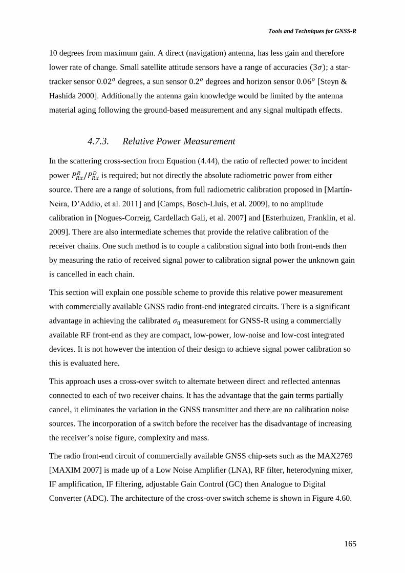
Tools and Techniques for GNSS-R
165
10 degrees from maximum gain. A direct (navigation) antenna, has less gain and therefore
lower rate of change. Small satellite attitude sensors have a range of accuracies (3𝜎); a star-
tracker sensor 0.02𝑜 degrees, a sun sensor 0.2𝑜 degrees and horizon sensor 0.06𝑜 [Steyn &
Hashida 2000]. Additionally the antenna gain knowledge would be limited by the antenna
material aging following the ground-based measurement and any signal multipath effects.
4.7.3. Relative Power Measurement
In the scattering cross-section from Equation (4.44), the ratio of reflected power to incident
power 𝑃𝑅𝑥𝑅 /𝑃𝑅𝑥
𝐷 is required; but not directly the absolute radiometric power from either
source. There are a range of solutions, from full radiometric calibration proposed in [Martín-
Neira, D’Addio, et al. 2011] and [Camps, Bosch-Lluis, et al. 2009], to no amplitude
calibration in [Nogues-Correig, Cardellach Gali, et al. 2007] and [Esterhuizen, Franklin, et al.
2009]. There are also intermediate schemes that provide the relative calibration of the
receiver chains. One such method is to couple a calibration signal into both front-ends then
by measuring the ratio of received signal power to calibration signal power the unknown gain
is cancelled in each chain.
This section will explain one possible scheme to provide this relative power measurement
with commercially available GNSS radio front-end integrated circuits. There is a significant
advantage in achieving the calibrated 𝜎0 measurement for GNSS-R using a commercially
available RF front-end as they are compact, low-power, low-noise and low-cost integrated
devices. It is not however the intention of their design to achieve signal power calibration so
this is evaluated here.
This approach uses a cross-over switch to alternate between direct and reflected antennas
connected to each of two receiver chains. It has the advantage that the gain terms partially
cancel, it eliminates the variation in the GNSS transmitter and there are no calibration noise
sources. The incorporation of a switch before the receiver has the disadvantage of increasing
the receiver’s noise figure, complexity and mass.
The radio front-end circuit of commercially available GNSS chip-sets such as the MAX2769
[MAXIM 2007] is made up of a Low Noise Amplifier (LNA), RF filter, heterodyning mixer,
IF amplification, IF filtering, adjustable Gain Control (GC) then Analogue to Digital
Converter (ADC). The architecture of the cross-over switch scheme is shown in Figure 4.60.

166
Figure 4.60 Schematic of receiver architecture to perform relative calibration using a cross-over switch
The cross-over switch is placed into the chain prior to any part of the receiver front-end
components. This is to allow cancellation of the receiver noise figure and the gain which may
be subject to drift with temperature and so are considered as unknowns. The two receiver
chains, 1 and 2, are nominally identical but due to component and temperature variations
their gain and noise terms are treated as separate unknowns. By using two receiver chains, the
signal measurements are uninterrupted except for the brief switch-over time.
The RF front-end functionality has been grouped together into the block marked R. This
combines the LNA, RF filter, mixer, IF amplification and IF filtering. For this discussion of
signal amplitude, these are considered to have total gains (in each receiver) of, 𝐺1 and 𝐺2 and
noise figures, 𝑇𝑅,1 and 𝑇𝑅,2.
The Gain Control (GC) would usually be automatically controlled in a GNSS navigation
receiver, where the gain (𝐺𝑉,1 and 𝐺𝑉,2) are varied to keep the noise power constant. This
calibration scheme relies on being able to fix this gain between both states of the cross-over

Tools and Techniques for GNSS-R
167
switch. This is possible in some front-end devices, including the example MAX2769
[MAXIM 2007].
Following the GC the Analogue to Digital Converter (ADC) quantises the signal into
typically either 2 or 3 bits. The limited number of quantisation levels in commercial GNSS
receivers introduces a quantisation loss that is dependent on the incoming signal.
Finally the receiver correlators are used to measure the signal power and the noise power.
Using one of the receiver chains (number 1 is chosen arbitrarily), the direct signal power can
be determined,
�̂�𝐷 = 𝑃𝑅𝑥𝐷 𝐺𝑅𝑥
𝐷 𝐺1𝐺𝑉,1𝐺𝑞,1,𝐷 (4.45)
where the 𝑃𝑅𝑥𝐷 term is the incident power at the antenna, 𝐺𝑅𝑥
𝐷 the antenna gain and the
subsequent G terms are the unknown gains within each of the stages of the receiver as
described in Figure 4.60; from the amplifiers, filters and mixer (𝐺1), the variable gain AGC
(𝐺𝑉,1, ) and quantisation stage (𝐺𝑞,1,𝐷, 𝐺𝑞,1,𝑅). The quantisation losses are treated separately
for each of the signal inputs as the proposed scheme fixes the gain control, stopping the
automatic adjustment that usually optimises the quantisation loss. The variable gain being
fixed at, 𝐺𝑉,1, is then unknown but the same for both positions of the cross-over switch.
If the cross-over switch is set to the reflected signal, with the GC gain remaining unknown
but held fixed, then the measured reflection power is equivalently,
�̂�𝑅 = 𝑃𝑅𝑥𝑅 𝐺𝑅𝑥
𝑅 𝐺1𝐺𝑉,1𝐺𝑞,1,𝑅 (4.46)
By taking the ratio of these, the receiver’s R block and GC gains cancel
�̂�𝐷
�̂�𝑅=
𝑃𝑅𝑥𝐷 𝐺𝑅𝑥
𝐷 𝐺1𝐺𝑉,1𝐺𝑞,1,𝐷
𝑃𝑅𝑥𝑅 𝐺𝑅𝑥
𝑅 𝐺1𝐺𝑉,1𝐺𝑞,1,𝑅
=𝑃𝑅𝑥
𝐷 𝐺𝑅𝑥𝐷 𝐺𝑞,1,𝐷
𝑃𝑅𝑥𝑅 𝐺𝑅𝑥
𝑅 𝐺𝑞,1,𝑅
(4.47)
This can then be rearranged, to the desired measurement of the ratio of powers from direct
and reflected signals,

168
𝑃𝑅𝑥𝑅
𝑃𝑅𝑥𝐷 =
�̂�𝑅𝐺𝑅𝑥𝐷 𝐺𝑞,1,𝐷
�̂�𝐷𝐺𝑅𝑥𝑅 𝐺𝑞,1,𝑅
(4.48)
The remaining quantities are the measured power of the direct and reflected signals when the
receiver has the cross-over switch in each of the ‘up’ and ‘down’ states and the antenna gains
𝐺𝑅𝑥𝐷 , 𝐺𝑅𝑥
𝑅 .
Using this cross-over switch scheme, the ratio of reflected to incident power 𝑃𝑅𝑥𝑅 /𝑃𝑅𝑥
𝐷 can be
determined (and therefore 𝜎0) without it being necessary or possible to measure the absolute
signal powers 𝑃𝑅𝑥𝑅 , 𝑃𝑅𝑥
𝐷 , the receiver gains 𝐺1𝐺𝑉,1, the receivers system noise temperatures,
𝑇𝑅,1, or the antenna temperatures 𝑇𝐴𝑅, 𝑇𝐴
𝐷, all of which can be considered unknown.
In addition the quantisation losses of the ADC remain (expressed as gains: 𝐺𝑞,1,𝑅, 𝐺𝑞,1,𝐷)
which will be discussed next.
4.7.4. Power Measurement Through A Coarsely Quantised
Analogue To Digital Converter
The state of the cross-over switch affects the quantisation loss due to the different noise
temperatures for the ‘up’ and ‘down’ pointing antennas.
Commercially available GNSS radio front-end devices typically quantise the signal to only a
few discrete levels, yet achieve a perhaps surprisingly low degradation. Receivers typically
use 1 bit, 2 bit or 3 bit quantisation which has a minimum degradation of 1.96 dB, 0.5369 dB
and 0.1589 dB respectively [Bastide, Akos, et al. 2003]. This very coarse quantisation is
possible due to the GNSS signals being below the thermal noise floor, spread over a wide
bandwidth by the PRN spreading code. Retrieval of the signal power is only possible after
correlating the signal out of the noise with a noise-free replica of the signal. The correlation
averages the signal over thousands of samples and thus the measurement resolution has much
finer quantisation levels due to the effective over-sampling.
To compare the effects of quantisation on signal power measurements, 1 bit, 2 bit, 3 bit and 4
bit idealised ADCs have been simulated with the responses as shown in Figure 4.61. Each
ADC has an output scaled to [-1, +1] to allow comparison.

Tools and Techniques for GNSS-R
169
Figure 4.61 ADC quantisation input and output values for different ADC accuracies. Output scaled to the
range [–1, +1]
To determine the signal power at the input to the ADC from the measurement at the output,
the following model for the GNSS signal, 𝑠(𝑡), with modulation code 𝑚(𝑡) will be
employed. This is the spreading code modulating the carrier at intermediate frequency f, and
input noise 𝑛(𝑡).
𝑠(𝑡) = 𝐴 𝑚(𝑡) e2𝜋𝑗𝑓𝑡+𝑗𝜙 + 𝐵𝑛(𝑡) (4.49)
The approach used assumes a linear system so that a single component of the GNSS signal
can be used to probe the response. The ADC only approaches a linear response in the over-
sampled regime in which we are operating. The signal definitions defined for crossing the
ADC are shown in Figure 4.62.
Figure 4.62 Quantisation model

170
The desired measurement is the signal power before the ADC, 𝐴2. As the spread signal is
below the noise power, 𝐵2, the signal measurement is carried out by multiplying by the
replica and integrating, as is typical with GNSS signals. If we could get to the analogue signal
before the ADC, then the signal integration would be
𝑤 =
1
𝑇∫ [(𝐴 𝑚(𝑡)e2𝜋𝑗𝑓𝑡+𝑗𝜙 + 𝐵 𝑛(𝑡))𝑚(𝑡)e2𝜋𝑗𝑓𝑡]
𝑇
0
𝑑𝑡 (4.50)
for a single integration period T seconds.
𝑤 =
1
𝑇∫ [𝐴 𝑚2(𝑡)(e2𝜋𝑗2𝑓𝑡+𝑗𝜙 + e𝑗𝜙) + 𝐵 𝑚(𝑡)e2𝜋𝑗𝑓𝑡𝑛(𝑡)]
𝑇
0
𝑑𝑡 (4.51)
𝑤 =
1
𝑇∫ [𝐴 e𝑗𝜙 + 𝐵 𝑚(𝑡)e2𝜋𝑗𝑓𝑡𝑛(𝑡)]
𝑇
0
𝑑𝑡 (4.52)
Now the integral is performed, the magnitude squared to get power and the noise components
are grouped into the new term 𝑛𝑤. This is the integral of the band-limited noise that passes
through the matched filtering. We now scale the whole result so that, 𝑛𝑤, has a standard
deviation of 1. The post correlation power terms, will be called, A’ and B’ for signal and
noise,
|𝑤| =
1
𝑇(𝐴′ + 𝐵′𝑛𝑤)
(4.53)
The equivalent can be performed for the post-quantisation signal, using 𝑠𝑞(𝑡), which gives
|𝑤𝑞| =
1
𝑇(𝐶′ + 𝐷′𝑛𝑤)
(4.54)
For the calibration correction we need the effect on the signal power of the GNSS component
due to the ADC response, i.e. 𝐺𝑞,𝑖 or 𝐴′2/𝐶′2. As the channel is dominated by noise, this will
depend on the input noise power to the ADC.
In the normal operation of a navigation receiver, the AGC continuously varies the gain to
keep the noise at the optimum power for the ADC and the quantisation loss will be the values
reported by [Bastide, Akos, et al. 2003]. In the proposed calibration scheme the gain will not
always be at the optimum setting, as it is necessary to hold the gain constant when the

Tools and Techniques for GNSS-R
171
receiver switches between antennas targeting the direct (D) and reflected (R) paths. The
receiver is cycled through exposure to antenna temperatures 𝑇𝐴𝑅 and 𝑇𝐴
𝐷.
This signal component model is simulated numerically to allow determination of the input
power to the ADC from the output samples. This would then allow measurement of the
received power ratio, in Equation (4.48), and from that the absolute radar scattering cross-
section.
With sufficient number of averaged measurements the remaining noise in the measurement
estimate B’ and D’ will decrease and we can determine the calibration correction in the limit
of a large number of measurements,
𝐺𝑞 =
|𝑤|2
|𝑤𝑞|2
(4.55)
This approach differs to the usual in GNSS navigation, which typically report signal-to-noise
ratio. In the GNSS-R application the interest is in calibrating the signal component through
the ADC; the noise level does not bias the power measurement, it only provides variance to
the estimate.
To parameterise the effects from changes in input noise power, the total RMS noise power is
calculated from the sampled signal, over N samples, both pre-quantisation,
𝑃 =1
𝑁∑(𝑠𝑖 − �̅�)2
𝑁
𝑖=1
(4.56)
and for the quantised signal,
𝑃𝑞 =1
𝑁∑(𝑠𝑞𝑖
− 𝑠�̅�)2
𝑁
𝑖=1
(4.57)
These include the GNSS component power, but in these simulations the GNSS component is
chosen to have 𝐶/𝑁0= 20 dB-Hz to be representative of the weak reflected signal. In the limit
that the signals are weak, 𝐴 << 𝐵 and 𝐶 << 𝐷 then the RMS power approaches that of the
noise only 𝑃 = 𝐵 and 𝑃𝑞 = 𝐷.
The post-quantisation measurement of the GNSS component power varies with the input
noise power, as determined from simulations of this model and shown in Figure 4.63. The
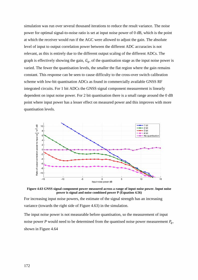
172
simulation was run over several thousand iterations to reduce the result variance. The noise
power for optimal signal-to-noise ratio is set at input noise power of 0 dB, which is the point
at which the receiver would run if the AGC were allowed to adjust the gain. The absolute
level of input to output correlation power between the different ADC accuracies is not
relevant, as this is entirely due to the different output scaling of the different ADCs. The
graph is effectively showing the gain, 𝐺𝑞, of the quantisation stage as the input noise power is
varied. The fewer the quantisation levels, the smaller the flat region where the gain remains
constant. This response can be seen to cause difficulty to the cross-over switch calibration
scheme with low-bit quantisation ADCs as found in commercially available GNSS RF
integrated circuits. For 1 bit ADCs the GNSS signal component measurement is linearly
dependent on input noise power. For 2 bit quantisation there is a small range around the 0 dB
point where input power has a lesser effect on measured power and this improves with more
quantisation levels.
Figure 4.63 GNSS signal component power measured across a range of input noise power. Input noise
power is signal and noise combined power P (Equation 4.56)
For increasing input noise powers, the estimate of the signal strength has an increasing
variance (towards the right side of Figure 4.63) in the simulation.
The input noise power is not measurable before quantisation, so the measurement of input
noise power P would need to be determined from the quantised noise power measurement 𝑃𝑞,
shown in Figure 4.64

Tools and Techniques for GNSS-R
173
Figure 4.64 Output noise power from ADC given range of input noise power. Input power is ratio
(expressed in dB) of the ideal RMS noise power for each of the n-bit ADCs.
The required ADC quantisation accuracy is determined by the dynamic range needed by the
cross-over switch calibration scheme. The noise difference between the two cross-over switch
states corresponds to 𝑇𝐴𝑅 = 𝑇𝑒𝑎𝑟𝑡ℎ and 𝑇𝐴
𝐷 = 𝑇𝑠𝑘𝑦. The input-equivalent noise for receiver 1
is,
𝑃𝑠𝑘𝑦 = 𝑘𝑏(𝑇𝑠𝑘𝑦 + 𝑇𝑅,1)𝐵
𝑃𝑒𝑎𝑟𝑡ℎ = 𝑘𝑏(𝑇𝑒𝑎𝑟𝑡ℎ + 𝑇𝑅,1)𝐵
where 𝑘𝑏 is the Boltzmann constant and B the noise bandwidth. By taking the worst case of
cold sky and tropical ocean, 𝑇𝑠𝑘𝑦 = 4 K, 𝑇𝑒𝑎𝑟𝑡ℎ = 300 K and the system noise temperature
of 273 K we find that the required noise power range is
10 log10𝑃𝑠𝑘𝑦
𝑃𝑒𝑎𝑟𝑡ℎ= −3.2 dB
Comparing this noise range to the signal power vs. input noise power in Figure 4.63, it is
desirable for the curve to be as flat as possible, as this means that the calibration is less
sensitive to error in measuring the input noise. It can be seen that the gain should be fixed at
the ideal point for the higher noise reflected path as the degradation is worse when over-
driving the ADC causing clipping of the input. This way when the cross-over switch is turned
to the direct signal, the input noise remains in the region that is closest to the ideal.
It is the noise power estimate at the output of the ADC, 𝑃𝑞, that is measureable by the
receiver. It is therefore the variance in this measurement that determines the achievable
calibration accuracy. Figure 4.65 shows the degradation in the GNSS signal component
power estimate over the range of measured output noise power.

174
Figure 4.65 Change in measured GNSS component power with measured output power
From the slope Δ𝐺𝑞/Δ𝑃𝑞 of Figure 4.65, the calibration sensitivity to the output noise
measurement can be determined. The achievable calibration accuracy is shown in Table 4.4
Table 4.4 Calibration accuracy achievable due to ADC
ADC quantisation
Accuracy of determining GNSS
component power given Δ𝑃𝑞 dB error in
output power measurement
2 bit 0.2 Δ𝐺𝑞 when -4 dB < 𝑃𝑞 < 0 dB
3 bit 0.1 Δ𝐺𝑞 when -5 dB < 𝑃𝑞 < 1 dB
4 bit 0.01 Δ𝐺𝑞 when -13 dB < 𝑃𝑞 < 2 dB
This is the best achievable calibration performance with the ADCs of very limited-
quantisation level as found in GNSS receiver electronics. From this it is clear there is a large
improvement in going from 3 bit to 4 bit sampling.
A further difficulty is that the direct antenna is not looking up at a clear, cold sky. Instead
there will typically be around 6-12 visible GPS satellites, and an increasing number of
Galileo satellites transmitting in-band. This is a dynamic situation as the interfering satellites
change relative positions, orientation and velocities. As these are all spread spectrum signals,

Tools and Techniques for GNSS-R
175
they would appear like white noise to the ADC and are expected to minimally affect the 𝐺𝑞
term.
To summarise this section, the scattering cross-section depends on the ratio of reflected to
incident signal power. A method of determining this has been presented that uses a cross-over
switch to eliminate variations in transmission power and cancel the receiver’s unknown gain
and noise. Table 4.5 summarises the estimates for the error sources for a GNSS-R receiver
using the cross-over switch scheme.
Table 4.5 Surface reflectance error estimates
Error source: Magnitude of
expected variation:
Direct-path receiver antenna gain knowledge,
combined with attitude determination
accuracy
0.3 dB
Reflected-path receiver antenna gain
knowledge, combined with attitude
determination accuracy
0.3 dB
Cross-over-switch calibration of receiver
gain
0.1 dB
GPS transmit power (due to small angle
between reflection and direct paths)
< 0.1 dB
Atmospheric path loss 0.1 dB
The variance in transmission power has been eliminated, which can vary by several dB
[Fisher & Ghassemi 1999] between satellites. The antenna gain knowledge and remaining
implementation aspects such as cable losses and impedance miss-matching provide the limit
to the achievable calibration accuracy.
The need for the GNSS-R receiver to measure the power ratio depends on the intended
surface measurement approach. The focus of this research is on ocean roughness
determination, for which the Z-V model of GNSS-R scattering shows that the normalised
DDM, and hence normalised 𝜎0, has sensitivity to ocean mean-square slope. The calibration
accuracy combined is estimated to be approximately 1 dB for the presented system. This is
about a 1/15th
of the modelled 11.9 dB range between the calmest and roughest ocean
conditions.

176
The technique presented here is one possible method to measure the relative signal power
from two separate antennas, this allows for a calibrated scatterometric surface measurement
using commonly available commercial GNSS radio frequency down-conversion chipsets and
a cross-over switch.
4.8. Discussion of the Software Receiver
Geometric tracking has been implemented in a software receiver for post-processing raw
GNSS-R data. Using this approach, correlators were steered to the delay and Doppler of
surface reflections to either generate DDMs or perform Stare processing. The improved
specular point calculations and the geometric tracking were shown to be sufficiently accurate
to allow on-board processing of reflections on a satellite receiver without having to perform a
search or acquisition stage to find the reflected signal.
The development of the software receiver has opened the opportunity for new analysis of the
UK-DMC data sets, as for the first time the complete archive has been processed and the
geometric tracking approach has found many more reflections. This is now being made
available for other organisations to study.
The software receiver was used to develop an optimal processing technique for the open-
service Galileo E1 signals through combining the sub-signals. This has led to the first
Galileo-type signal reflection to be detected from orbit. A dual, GPS-Galileo capable GNSS-
R receiver has the opportunity to target twice the number of specular points and so double the
coverage from one receiver. The contribution of a practical receiver architecture for
processing these Galileo-like signals will become increasingly relevant as the modernising
GNSS services include more complex signal specifications.
The work presented on Stare processing is based on the SHARP approach proposed by
Starlab, of Barcelona. The research here is the first detailed investigation to be published,
tackling the practical implementation challenges and additionally provides a demonstration
on spaceborne data. In particular the most significant contribution has been in applying the
radar equation to adapt the measurement of the scattering cross-section as the geometry of the
reflection changes through the observation. The results from the UK-DMC experiment
demonstrate the technique can be practically implemented. An implementation of the Z-V
scattering model has been used to determine the sensitivity of Stare processing to the ocean

Tools and Techniques for GNSS-R
177
surface roughness. The limited dataset from UK-DMC, was insufficient to build a semi-
empirical model to invert these scattering cross-section measurements into ocean roughness.
The GNSS-R community requires more data from orbit to be able to build an ocean
roughness retrieval model. The Stare processing technique is one option which shows merit
as it has an output that is closer to that of the traditional monostatic scatterometers, the
resolution on the ocean surface is improved over that from DDM processing and a lower
downlink data rate is needed.
The sections of this chapter combine to form a number of improvements to a GNSS-R sensor.
Firstly the improved specular point calculation provides better geo-location and enables real-
time processing through geometric tracking. Next the receiver coverage is improved through
the additional measurement points made available by Galileo-Reflectometry. In addition
through the Stare processing work, improvements were made to the surface resolution, and
the down-link rate of a receiver. Finally a calibration scheme was developed to improve the
retrieval accuracy of surface roughness.
The software receiver’s automated processing makes it suitable for the new data sets that will
be collected by the SGR-ReSI receiver when launched on TechDemoSat-1. This means that it
will additionally aid in the validation of GNSS-R in the next generation of receiver, so
continue to contribute to towards an operational instrument for ocean roughness
measurement.

178
Chapter 5: Real-Time Processing
The previous chapter developed some of the techniques required for processing of reflected
GNSS signals and detailed new processing techniques. The demonstration and testing were
carried out with a software receiver on the limited data set collected by the UK-DMC
satellite. Spaceborne GNSS-R is in the validation stage at the time of this PhD, as the
performance in terms of resolution, bias and variance of geophysical measurement techniques
has not been demonstrated. There are still a number of competing techniques. It is considered
that the greatest problem to be solved in the area of GNSS-R at the time of this project is the
collection of more data to build an empirical retrieval algorithm informed by the existing
scattering models.
A new satellite instrument that is capable of collecting the data for validation of GNSS-R is
needed. The previous chapter looked back at what could be learnt from the UK-DMC data-
sets. This chapter looks forward to specifying, designing and building the next generation of
instrument from the lessons learnt from the UK-DMC experiment. In particular, to get the
quantity of data required for validation of ocean roughness measurement, many more
collections need to be downlinked from the satellite. The innovations developed in this
chapter solve this through data reduction by on-board processing and real-time tracking of
GNSS reflections.
5.1. Motivation
The ocean surface conditions can roughly be considered stationary for a time of 4 hours
[Sarkar, Basu, et al. 2002], but many altimeter satellites have a repeat ground track interval of
several days. To achieve measurement of the ocean with a complete, global picture within
these temporal sampling requirements, the only practical solution is a constellation of remote-
sensing satellites. To realise such a system the cost of each sensor needs to be minimised.
The instrument development was carried out at the Surrey Space Centre department of the
University of Surrey, under co-sponsorship from Surrey Satellite Technology, both groups
specialise in small, low cost satellites. This has influenced the aim to produce a GNSS
reflectometry receiver that is compatible with these system requirements.

Real-Time Processing
179
There is typically a GPS receiver on a satellite as part of the platform for providing timing
and position for the satellite’s payload. Making the platform GPS receiver capable of GNSS-
R measurements would allow sharing of hardware and provide a low cost additional remote
sensing capability, or add value to the satellite for its customers. The goal is to produce a
receiver that effectively acts as a secondary payload which means that for it to be an
attractive device for a customer it should have a minimal impact on the platform and primary
payload. A rapid deployment of a GNSS-R constellation would then be possible by
deployment on a constellation, for example RapidEye, built by SSTL and launched in 2008,
Figure 5.1.
Figure 5.1 SSTL supplied 5 multispectral ground-imagery satellites for the RapidEye constellation in
2008. (Courtesy: Surrey Satellite Technology)
The GNSS-R instrument needs to meet the constraints of a small satellite platform, of which
the most significant are the mass, power, data rate and antenna size limitations. However the
design goal goes beyond meeting the payload requirements of a small satellite but instead
aims to be a fraction of the main payload requirement, so that it is an attractive secondary
payload. To make the payload an attractive proposal for a secondary payload on a typical
100 kg or 150 kg class microsatellite, then the payload mass should be less than 5 kg, power
consumption less than 10 W, continuous data rate less than 500 Kibit/s and an antenna within
a 40 cm by 40 cm square. These requirements would vary depending on the hosting platform
and specifications of other payloads, but it does give a useful envelope within which to set
bounds for a GNSS-R receiver design.
This thesis has been working towards a GNSS-R receiver system for SSTL’s SGR-ReSI
(Space GNSS Receiver Remote Sensing Instrument) as introduced in Section 2.4.1. During
the course of this research the SGR-ReSI was selected amongst a number of other technology

180
demonstration payloads for launch on the TechDemoSat-1 (TDS-1) satellite. This platform is
based on the SSTL-150, which is similar to that used for the RapidEye constellation. The
selection of this specific platform has further defined some of the receiver constraints on
interfaces, operations and antenna. A picture of the SGR-ReSI Flight module is shown in
Figure 5.2
Figure 5.2 SGR-ReSI flight model
The most challenging aspect is to achieve the data downlink rate and the link-margin given
the antenna constraints. The link margin was approached in the previous chapters. This
chapter focuses on an approach to reduce the rate that data is produced and forwarded to the
ground.
5.2. Processing Split Between Satellite and Ground
Ideally the satellite would process measurements and continuously derive the surface
roughness measurement directly on-board. However as the inversion procedure has not been
validated, it is vital that a GNSS-R instrument has the flexibility to process the signal in a
number of ways. The most flexible approach would be to downlink the raw intermediate
frequency (IF) samples. Continuously recording raw IF 2 bit samples and storing on the
satellite from nadir and zenith front ends, at a sample rate of 16 MHz, would accumulate
around 6000 Gb (bits) per day, a data-rate that is incompatible with small satellites or hosted
payloads. The TDS-1 platform is capable of downlinking about 700 Gb per day (assuming
one ground station and 650 km altitude).
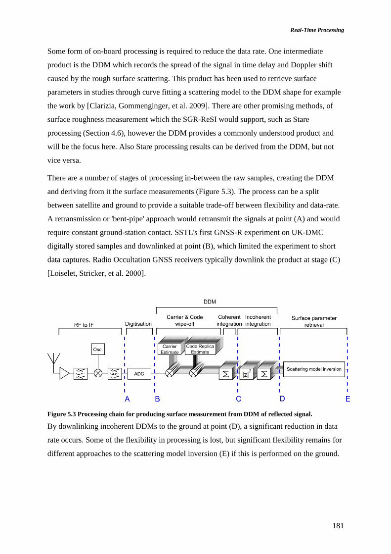
Real-Time Processing
181
Some form of on-board processing is required to reduce the data rate. One intermediate
product is the DDM which records the spread of the signal in time delay and Doppler shift
caused by the rough surface scattering. This product has been used to retrieve surface
parameters in studies through curve fitting a scattering model to the DDM shape for example
the work by [Clarizia, Gommenginger, et al. 2009]. There are other promising methods, of
surface roughness measurement which the SGR-ReSI would support, such as Stare
processing (Section 4.6), however the DDM provides a commonly understood product and
will be the focus here. Also Stare processing results can be derived from the DDM, but not
vice versa.
There are a number of stages of processing in-between the raw samples, creating the DDM
and deriving from it the surface measurements (Figure 5.3). The process can be a split
between satellite and ground to provide a suitable trade-off between flexibility and data-rate.
A retransmission or 'bent-pipe' approach would retransmit the signals at point (A) and would
require constant ground-station contact. SSTL's first GNSS-R experiment on UK-DMC
digitally stored samples and downlinked at point (B), which limited the experiment to short
data captures. Radio Occultation GNSS receivers typically downlink the product at stage (C)
[Loiselet, Stricker, et al. 2000].
Figure 5.3 Processing chain for producing surface measurement from DDM of reflected signal.
By downlinking incoherent DDMs to the ground at point (D), a significant reduction in data
rate occurs. Some of the flexibility in processing is lost, but significant flexibility remains for
different approaches to the scattering model inversion (E) if this is performed on the ground.

182
5.2.1. Comparison With a Navigation Receiver “Cold Search”
It is insightful to compare the DDM in GNSS-R to the search space in a navigation receiver,
so that existing techniques can be evaluated. Before tracking GNSS signals a navigation
receiver must firstly search through code delay and carrier frequency to acquire these signals
hidden in the noise. The size of the search space depends on the GNSS code length, chipping
rate, the user velocity and the receiver clock uncertainty. The frequency search range for a
ground based receiver is based primarily on the range of receiver velocities; while the code
search space is carried out typically at 0.5 chip steps to limit the maximum loss associated
with misalignment to –3 dB. The frequency search is ±10 kHz in steps of 500 Hz [Borre,
Akos, et al. 2006], limiting the misalignment loss to a further –3 dB.
This leads to a search space of 1023 · 2 ∙ (20 × 103)/500 = 81,840 combinations or delay
‘pixels’ if considered as a DDM.
The correlation output formed in the navigation receiver’s acquisition stage is immediately
discarded as the peak provides the location of the signal to initialise the tracking of the signal.
Accordingly the pixels can be searched serially, in parallel or a combination of blocks
depending on the hardware available for processing. For GNSS reflectometry, it is the
recording of the values in this search space that is desired, and therefore all the pixels are
required to be recorded simultaneously.
The delay-Doppler map of the reflection is analogous to the GNSS acquisition search space.
It is assumed that the reflection specular point is at a known pseudo-range and carrier
frequency, so the signal is already ‘found’ in this signal space. However the term ‘search
space’ is still used to help show the analogy to the GNSS acquisition problem. The spread of
the signal from the reflection is determined by the physical size of the scattering zone on the
surface, the geometry of the transmitter, receiver and their velocities. Additionally the link-
budget determines how far from the specular point a signal will have sufficient SNR for
detection.
The range of delays and Doppler that would be expected from the surface could be
determined from a surface scattering model combined with link-budget calculations.
However it is not clear that the current models have been effective at predicting the absolute
power levels so the approach will be taken to use information derived from the results of the
UK-DMC experimental GNSS-R receiver. The parameters of the UK-DMC GNSS-R
experiment are described in Section 3.2. Through all the measurements taken the antenna was

Real-Time Processing
183
kept pointing away from nadir by 10 degrees. This means that the reflections had largely the
same delay and Doppler characteristic shape with a Doppler frequency spread of around
10 kHz and a spread in delay up to about 30 μs. The DDM in Figure 5.4 is typical of the
reflections processed from UK-DMC. This spread is considerably less than the search space
for navigation receiver acquisition but considerable greater than that used in signal tracking.
Figure 5.4 A UK-DMC reflection processed using the software receiver. Colour scale is chosen to provide
a measure of reflection detectability. Processing as described in Section 4.1.
5.2.2. Sampling Resolution
Without a full and finalised retrieval technique to go from DDM to an estimate of the Earth
surface roughness, the most appropriate way to determine the required sampling intervals for
delay and Doppler is to consider the properties of the ambiguity function.
Over-sampling of the ambiguity function wastes computational effort for no gain in
information, whereas under-sampling will produce gaps where signal power and therefore
information is lost. From the shape of the GPS C/A code ambiguity function which is shown
in Figure 2.6, the maximum losses can be calculated for the ambiguity function and have
been listed in Table 5.1 for Doppler and Table 5.2 for delay.

184
Table 5.1 Maximum loss with different sampling resolutions in Doppler dimension
Frequency Spacing
[Specific case 𝑻𝒄𝒐𝒉 = 1 ms]
Power Loss (dB)
2/𝑇𝑐𝑜ℎ = [2000 Hz] -inf. (due to null)
1/(𝑇𝑐𝑜ℎ) = [1000 Hz] -3.9
1/(2𝑇𝑐𝑜ℎ) = [500 Hz] -0.9
1/(4𝑇𝑐𝑜ℎ) = [250 Hz] -0.2
Table 5.2 Maximum loss with different sampling resolutions in delay dimension
Delay Spacing
[Specific case 𝑻𝒄 = 978 ns]
Power Loss (dB)
1 𝑇𝑐 = [978 ns] -6.0
1/2 𝑇𝑐 = [489 ns] -2.5
1/4 𝑇𝑐 = [244 ns] -1.15
1/8 𝑇𝑐 = [122 ns] -0.6
By choosing frequency and delay resolutions of 1/(2𝑇𝑐𝑜ℎ) and 1/4 𝑇𝑐 respectively, the DDM
will be sampled sufficiently that it will be within 2 dB of a continuous representation of the
DDM. Alternatively, choosing improved resolutions of 1/(4𝑇𝑐𝑜ℎ) and 1/8 𝑇𝑐, the DDM will
be sampled sufficiently to be within 1 dB of the continuous DDM. The smoothing effect of
the ACF leads to diminishing returns when improving the DDM sampling resolution, with
very closely spaced samples being highly correlated.
The summary of the comparison between GNSS navigation and reflectometry requirements is
shown in Table 5.3. The required DDM resolution has been specified for a maximum
sampling induced power error of 1 dB. This value is thought to be suitable, but it is expected
that different inversion techniques will have different sensitivity to the sampling resolution.
The specifications of the reflectometry processor are considerably different to that of the
navigation receiver, both in the search space, the resolution and most significantly in the
requirement for the full DDM result to be calculated continuously at the rate of 1/𝑇𝑐𝑜ℎ.
The sampling frequency is taken to be 𝑓𝑠=16.367 MHz as this provides sufficient Nyquist
bandwidth for an anti-aliasing filter with wide transition band and low group delay variation;
additionally this is a commonly supported frequency among RF front-end chip-sets.

Real-Time Processing
185
Table 5.3 Reflectometry DDM processor requirements compared to navigation cold search.
Navigation cold-search Reflectometry
Delay Range 1023 chips 30 chips
Delay Resolution 0.5 chips 0.125 chips
Number of delay pixels 2048 240
Doppler Range 80 kHz (for orbiting receiver) 10 kHz
Doppler Resolution 50 Hz to 500 Hz depending
on coherent integration
period
250 Hz maximum
Number of Doppler pixels 160 to 1600 40
Coherent integration
period
Typically 1 ms to 10 ms Around 1 ms (depending on
receiver and transmitter
relative locations)
Processing time for one
complete coherent map
Under 1 minute typical Continuous, 1 ms
Number of simultaneous
PRNs
1 4 (From Section 3.6)
With a chosen DDM sampling resolution the requirements for the capacity of the satellite
downlink rate can be determined for each reflectometry channel. By generating 1 second
integration DDMs of the ocean once a second, with resolution 240 x 40 pixels, and 10 bit
quantisation per pixel, then a 96 Kibit/s data stream is produced, or 8.3 Gb per day per
reflection. The DDM is effectively a picture, which could be compressed, or only parts
selected for downlink, so this is not necessarily the minimum rate, but gives an upper bound
of what needs to be supported per reflection channel.
5.3. Existing Work
There are two areas with potential similarity to the DDM calculation problem, these are in the
field of GNSS acquisition as already summarised. In addition there are other GNSS-R
instruments under development which were listed in Section 2.5. Of these airborne and
ground-based instruments, some are capable of real-time processing: UPC’s PAU-OR,
IEEC’s GoldRTR and Starlab’s Oceanpal (Section 2.5). However the significant difference to
this project is that they have been designed for airborne or ground platforms rather than for a
satellite platform. This has a large influence on the processing specifications. Ground and
airborne receivers do not have the same power, mass, environmental and data rate limitations
as satellite instruments. In terms of the processing there is virtually no Doppler spread
apparent in an airborne receiver and the signal is spread over a smaller range of delays. This
results in a significantly reduced computational challenge.

186
5.4. Processing Architecture
The chosen architecture of the DDM processing is the Field Programmable Gate Array
(FPGA). This is an integrated circuit consisting of programmable logic blocks and
reconfigurable interconnects that allow the blocks to be wired together to form complex
functions. The design of which is specified in a Hardware Description Language (HDL). In
addition to reconfigurable logic elements, dedicated resources such as memory and Digital
Signal Processing (DSP) elements, usually addition and multiply units are included. The
parallelism of the resources on an FPGA allows for considerable throughput in high
performance computing applications and can offer order of magnitude performance
improvements over a software implementation running on a microprocessor. The
parallelisation can be used to reduce the clock rate and hence the power consumption. The
downside of this performance is that the design process is considerably more complicated
than that of software implementations.
The FPGA was selected as the target technology as processing an array of pixels in the DDM
is particularly suited to the parallel nature of the FPGA. The method of trading off the
complexity of the processing approaches is significantly different from that taken for
software implementations. For a microprocessor, the hardware performance is typically
estimated by the number of multiplies or additions per second, as there is normally just a
single hardware ‘arithmetic unit’ that will perform these operations serially. Each operation
being equally expensive to perform in terms of time and power consumption, the number of
multiply and addition operations required provides a reasonable measure of algorithmic
complexity.
An FPGA can exploit the parallelism in an algorithm by implementing many multiplier and
adder units, each one programmed into the hardware. The adders and multipliers are either
provided by the reconfigurable logic or dedicated, fixed structures within the chip. The
reconfigurable logic implementations use fewer resources for lower precision integers which
are represented with fewer bits. Unlike a software implementation that typically has access to
a large Random Access Memory (RAM), an FPGA has a limited amount of fast on-board
RAM and otherwise must connect to slower external RAMs. In addition the logic resources
can be used multiple times per input sample, so running at a higher clock rate to increase the
number of operations that can be performed per sample. Due to these characteristics in an
FPGA, a more complex approach is needed for trade-off of different processing approaches
to that in software. The approach we shall take is to calculate the FPGA capacity needed by

Real-Time Processing
187
the number of multiplies required per input sample per second. The cost of the multiplies will
be scaled by the precision of the integers required.
The following analysis is based on the Xilinx devices [Xilinx 2011] using the Virtex-4
technology series, but is equally applicable to devices from other manufacturers. The
reprogrammable logic is made up from an array of reprogrammable 4 input Look-Up-Tables
(LUTs). The number of LUTs is limited on each integrated circuit and provides the limit to
the number of DDM pixels that can be calculated. The resource utilisation was calculated for
a range of arithmetic units on the target Xilinx Virtex-4 FPGA with varying operand width
(Figure 5.5). Multiplier circuits require significantly more logic resources than an adder
circuit. Therefore the adders can effectively be ignored in the complexity analysis.
Figure 5.5 FPGA resource utilisation on Virtex-4 series devices from Xilinx for circuits that perform
A*B=C and A+B=C. The number of bits used to represent A and B is varied to show the influence of the
calculation precision.
From this graph a curve of best fit was produced for the resource usage of the two arithmetic
circuits. These will be used in assessing the algorithm design. The number of LUTs for input
precision of 𝑁𝑏 bits is:
LUTs used in multiplier = 1.41 ∙ 𝑁𝑏1.95
LUTs used in adder = 𝑁𝑏
A mid-range Digital Signal Processing FPGA used in the SGR-ReSI, made by Xilinx
contains 30,700 of the 4-input Look-Up Tables.
0
200
400
600
800
1000
1200
1400
0 8 16 24 32
Nu
mb
er o
f 4
-in
pu
t L
oo
k-U
p-T
ab
les
Operand bit width
(Number of bits)
Multiplier
Adder

188
5.5. Time-Domain Techniques
Each pixel of the DDM is calculated as a matched filter of the transmitted signal with an
estimate of the carrier frequency and code delay as in Section 2.2.1. The calculation for a
single pixel is shown diagrammatically in Figure 5.6. Following coherent matched filtering,
the incoherent sum is performed to average the noise from the weak and relatively incoherent
reflections.
Figure 5.6 Forming a single pixel in the DDM, using time domain approach
To provide a basis for the estimate of the resources used and to help constrain the design
analysis, the DDM resolution and sampling characteristics from Section 5.2.2 will be used to
analyse this approach as a solution to real-time processing on-board the remote sensing
satellite.
An analysis of the resource utilisation in an FPGA for this algorithm requires analysis of the
precision of the calculation, which is the number of bits at each stage. It will be assumed that
the input is a 3 bit value and subsequent stages avoid any rounding. Accumulators are
particularly sensitive to rounding errors, so this is a reasonable assumption for the design
analysis.
Each discrete correlator has the following resources: a 3 bit by 1 bit multiplier for the
incoming signal multiplied by code replica. Then carrier multiplication, I and Q, each 3 bit by
3 bit forming a 6 bit result. Coherent accumulation and incoherent accumulation each
increase the bit width substantially due to the number of accumulations before resetting the
counter. Coherent accumulations number 𝑓𝑠 ⋅ 𝑇𝑐𝑜ℎ = 16,367 from the specifications in Table
5.3, resulting in word growth to 20 bits. The calculation of the squared magnitude requires
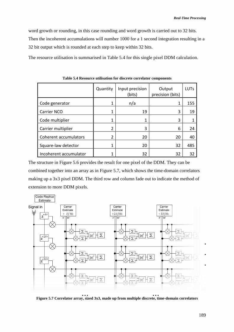
Real-Time Processing
189
word growth or rounding, in this case rounding and word growth is carried out to 32 bits.
Then the incoherent accumulations will number 1000 for a 1 second integration resulting in a
32 bit output which is rounded at each step to keep within 32 bits.
The resource utilisation is summarised in Table 5.4 for this single pixel DDM calculation.
Table 5.4 Resource utilisation for discrete correlator components
Quantity Input precision (bits)
Output precision (bits)
LUTs
Code generator 1 n/a 1 155
Carrier NCO 1 19 3 19
Code multiplier 1 1 3 1
Carrier multiplier 2 3 6 24
Coherent accumulators 2 20 20 40
Square-law detector 1 20 32 485
Incoherent accumulator 1 32 32 32
The structure in Figure 5.6 provides the result for one pixel of the DDM. They can be
combined together into an array as in Figure 5.7, which shows the time-domain correlators
making up a 3x3 pixel DDM. The third row and column fade out to indicate the method of
extension to more DDM pixels.
Figure 5.7 Correlator array, sized 3x3, made up from multiple discrete, time-domain correlators

190
To form a DDM processor in hardware from this structure, the resources for the multipliers
and adders are summed, under the assumption that the resources used in interconnections can
be neglected. To add generality for different receiver altitudes and geometries, the size of the
DDM processor will be parameterised, such that 𝑁𝑑 delay pixels by 𝑁𝑓 frequency pixels are
calculated, for 𝑁𝑅 different reflections.
Particular benefit is gained from resource sharing in the magnitude and incoherent
accumulation operations as these are calculated at a significantly lower rate. Once in
𝑇𝑐𝑜ℎ = 1 ms rather than the sample period of 1/𝑓𝑠 ≅ 60 ns. The correlator architecture with
resource sharing is shown in Figure 5.8
Figure 5.8 Correlator array resource sharing the incoherent accumulations
Further resource sharing could be achieved by reusing the carrier and code multipliers at a
multiple of the sample clock rate, although this would require more resources for the
switching and intermediate result storage and is more challenging to calculate. It can be seen
from the architecture in Figure 5.8 that the number of LUTs needed is increasing rapidly with
the number of pixels. The resource estimate of this DDM calculation array is combined with
the estimates from Table 5.4 to determine whether this algorithm is feasible for

Real-Time Processing
191
implementation. Figure 5.9 shows the resulting resource estimate in terms of the number of
LUTs used for this architecture and a variable DDM size.
(A) (B)
Figure 5.9 Number of LUTs used for discrete correlator array. (A) The horizontal surface indicates the
capacity of the reference Xilinx Virtex-4 SX35 chip of 30,700 LUTs. (B) Shows the view of this surface,
showing the DDM processor dimensions that would fit within the device.
These estimates are only for a single reflection; our requirements set out that 4 simultaneous
reflections must be mapped. These figures show that with the current technology, the
algorithm is not suitable for this application, as it would require 3 of the largest devices in the
Xilinx Virtex-4 series, which have 178,000 LUTs, for each of the 40 by 240 pixel reflections
to meet our requirements. This would have a very significant size, power and cost
implication, which is incompatible with the small satellite platform. The following sections
solve the computational challenge through development of a more efficient algorithm.
5.6. Frequency Domain Techniques
There are a number of algorithms for accelerated GNSS acquisition by transformation of the
signal into the frequency domain. The frequency domain can be used for the code delay
search or the carrier frequency search. The transformation provides a method of reducing the
computational complexity of one or more of the factors in the processing time for discrete
correlators, which go with the total number of pixels in delay, Doppler and number of
reflections as 𝑁𝑑 ∙ 𝑁𝑓 ∙ 𝑁𝑅
Number of Delay pixels
Num
ber
of
Dopple
r pix
els
20 40 60 80 100 120
5
10
15
20
25
30
35
40
Larger than
device
Fits in
device

192
(A) (B) (C)
Figure 5.10 Computing the DDM by individual pixel computation (A), or by transformation into the
frequency domain for calculation of lines of constant Doppler (B) or delay (C) lines simultaneously.
There is some difficulty in showing detailed methods used by some companies due to the
nature of the GNSS receiver industry focusing on commercial rather than academic
objectives. A good starting point is [Pany 2010, chap.9.5] or [Yang 2001], which describe
Fourier transform based approaches for software receivers to parallelise the computation in
either of the code delay or carrier dimensions. Either (B) or (C) of Figure 5.10.
There are a few papers that describe GNSS acquisition hardware: Septentrio have designed
the FAU (Fast Acquisition Unit), [De Wilde, Sleewaegen, et al. 2006] which uses an FFT for
the frequency search. Another implementation uses Fourier transforms in the code search
[Sajabi, Chen, et al. 2006].
5.6.1. Code Correlation in the Frequency Domain
A column of the DDM (fixed frequency) can be computed more efficiently by performing the
correlation in the frequency domain. For this we assume that the incoming signal has already
been down-converted to baseband, and sampled so is now,
𝒔𝑛 = 𝑐(𝑡 − 𝜏) exp(𝑗𝜙) (5.1)
where 𝑐 is the PRN code with propagation delay 𝜏 and residual phase, 𝜙. The DDM can be
calculated for a range of code delays by transforming the time-domain correlation through the
convolution theorem. This is re-derived here due to its importance to understanding the way
in which the frequency domain can be used to perform cross-correlation and to highlight the
equivalence and differences.
The derivation uses the inverse DFT of a signal, s, and the replica, r. The n index is the
sample number in the time domain representation of the signal.

Real-Time Processing
193
𝑠𝑛 =1
𝑁∑ 𝑠�̂�
𝑁−1
𝑘=0
e2πi𝑛𝑘𝑁
𝑠𝑛 =1
𝑁ℱ−1{𝑠�̂�}
(5.2)
𝑟𝑛 =1
𝑁∑ 𝑟�̂�
𝑁−1
𝑙=0
e2πi𝑛𝑙𝑁
𝑟𝑛 =1
𝑁ℱ−1{𝑟�̂�}
(5.3)
k and l are the frequency domain indices for the signal and replica respectively.
In the time domain, circular correlation can be written,
ℎ𝑚 = ∑ 𝑠𝑛𝑟𝑛+𝑚
𝑁−1
𝑛=0
(5.4)
where m is the offset in samples between the signal and replica. Substituting in the frequency
domain representation of r and s,
ℎ𝑚 = ∑1
𝑁∑ 𝑠�̂�
𝑁−1
𝑘=0
e2πi𝑛𝑘𝑁 ⋅
1
𝑁∑ 𝑟�̂�
𝑁−1
𝑙=0
e2πi𝑙(𝑛+𝑚)
𝑁
𝑁−1
𝑛=0
=1
𝑁2∑ ∑ 𝑠�̂�𝑟�̂�e
2πiN
𝑛𝑘+𝑙(𝑛+𝑚)
𝑁−1
𝑘,𝑙=0
𝑁−1
𝑛=0
(5.5)
Splitting out the sum over the sample index, n
=1
𝑁2∑ 𝑠�̂�𝑟�̂�e
2πiN
𝑚𝑙
𝑁−1
𝑘,𝑙=0
∑ e2πiN
𝑛(𝑘+𝑙)
𝑁−1
𝑛=0
(5.6)
This allows us to use the definition of the Kronecker delta (that 1
𝑁∑ 𝑒
2𝜋𝑖𝑛(𝑘+𝑙)
𝑁 =𝑁−1𝑛=0 𝛿𝑘,𝑙 and
𝛿𝑘,𝑙 = 1 when 𝑘 = 𝑙, otherwise 𝛿𝑘,𝑙 = 0)
=1
𝑁2∑ 𝑠�̂�𝑟�̂�e
2πiN
𝑚𝑙
𝑁−1
𝑘,𝑙=0
𝑁𝛿𝑘,−𝑙 (5.7)

194
=1
𝑁∑ 𝑠−�̂�𝑟�̂�e
2πiN
𝑚𝑘
𝑁−1
𝑘=0
(5.8)
Which is recognisable as an inverse DFT,
ℎ𝑚 = ℱ−1{𝑠−�̂�𝑟�̂�} (5.9)
So the time domain circular correlation can be calculated using the frequency domain
representations of the signal and replica. This can be written algorithmically as,
ℎ𝑚 =
1
𝑁ℱ−1{FLIP{ℱ{𝑠𝑛}} ⋅ ℱ{𝑟𝑛}}
(5.10)
And defining the function, FLIP{𝑠−�̂�} = 𝑠�̂�
The circular correlation result calculated using the frequency domain is therefore shown to be
identical to the time-domain calculation. The equivalence of this method means that the
computation can take advantage of the computationally efficient FFT implementations of the
DFT, to reduce the number of operations required. The flow of the baseband processing is
shown in Figure 5.11.
Figure 5.11 Frequency domain correlation (adapted from [Pany 2010] )
Unless the number of samples is a power of two then the correlation will not be circular, and
zero padding will be needed. In reality the GNSS signals are close enough to a power of 2 in
length that zero-padding need not be used if a small error is acceptable.

Real-Time Processing
195
This method has the advantage that all code phases are computed in parallel, but in the
GNSS-R application only 30 chips out of total 1023 chip C/A code are required, according to
the specification in Table 5.4. So by discarding 97.1% of the calculated results the
computational efficiency is relatively poor. The reflectometry application more closely
resembles the search space of a navigation receiver with some a-priori knowledge of the code
phase, such as could be used in assisted GNSS. An algorithm for limited code-phase search
has been proposed in [Sagiraju, Agaian, et al. 2006; Sagiraju, Raju, et al. 2008] but
introduces significant errors in signal power estimation away from the zero delay code phase.
Overlap-add or overlap-save are possible ways of getting around the waste of discarding the
unneeded results. However for the following reasons the frequency domain code correlation
was not selected as a viable approach for a practical GNSS-R receiver,
- From the table of resource usage in the discrete correlator Table 5.4, it is the carrier
multiplier that uses 24 times the LUTs than the code multiplication.
- A software receiver can cache the FFT of the code, so that this does not need to be
recalculated continuously. However there is insufficient RAM within an FPGA for
this and the required transmission bandwidth for storing off-chip is very high.
Without this storage the efficiency is decreased as the FFT operation is continuously
recalculated with the same input.
5.6.2. Doppler Search Using the Frequency Domain
An alternative approach performs the Doppler search in the frequency domain to reduce the
computation complexity (Figure 5.10 (C)). This is explained in more detail as it is the
approach that has been chosen for due to its suitability for implementation in an FPGA.
With reference to Figure 5.12: Firstly a coarse carrier ‘wipe-off’ is performed to down-
convert such that 0 Hz is the centre of the DDM, corresponding to the Doppler of the specular
path. This is followed by a set of channels that ‘wipe-off’ the code, each configured for the
delay of a separate DDM row. The result of the coarse carrier wipe-off and code wipe-off
leaves a demodulated signal at a small residual Doppler frequency. The small residual carrier
contains the full spectrum of Doppler shifts present for the chosen code phase and spectrum
estimation will return one column of DDM pixels simultaneously. This technique will now be
explained and evaluated for implementation in an FPGA.

196
A GNSS signal component, with the structure defined in Section 2.2.1, is modified by the
reflection from the Earth’s surface. Here a component is analysed which reflects from the
surface with an offset distance from the specularly point. This reflection point is physically
separated from the specular point and therefore the delay and Doppler are also offset. The
chosen surface point component has PRN spreading code, 𝑐(𝑡 − 𝜏𝑆 − Δ𝜏), where 𝜏𝑆 is the
propagation delay of the specular path and Δ𝜏 is the additional delay due to the additional
transmitter-Earth-receiver distance. Similarly the specular point is offset from the carrier
frequency, 𝑓𝐿, by 𝑓𝑆𝑃, and a point on the surface has an offset from this of Δ𝑓. This results in
a signal component where the specular path has Δ𝜏 = 0 and Δ𝑓 = 0,
𝑠(𝑡) = 𝐴 𝑐(𝑡 − 𝜏𝑆 − Δ𝜏) exp(𝑗2𝜋(𝑓𝐿 + 𝑓𝑆𝑃 − Δ𝑓)𝑡) (5.11)
We firstly multiply by the carrier NCO at the specular point intermediate frequency 𝑓𝐿 + 𝑓𝑆𝑃,
this down-converts the specular point signal to baseband. Ignoring high frequency terms, this
becomes
𝑢(𝑡) = 𝐴 𝑐(𝑡 − 𝜏𝑆 − Δ𝜏) exp(−𝑗2𝜋 Δ𝑓 𝑡 + 𝜙) (5.12)
This leaves the reflection component with a small residual Doppler, either side of the
specular ray at 0 Hz.
Then we multiply by the spreading code replica, 𝑐(𝑡 − 𝑡′),
𝑣(𝑡) = 𝐴 𝑐(𝑡 − 𝜏𝑆 − Δ𝜏) 𝑐(𝑡 − 𝑡′) exp(−𝑗2𝜋 Δ𝑓 𝑡 + 𝜙) (5.13)
We then assume a perfect code alignment, such that 𝜏𝑆 + Δ𝜏 = 𝑡′. In which case the
expectation of the spreading code multiplication is,
⟨𝑐(𝑡 − 𝑡′) ⋅ 𝑐(𝑡 − 𝜏0 − 𝑡′)⟩ = 1 (5.14)
and therefore the result becomes a complex sinusoid. So assuming identification of the
correct delay, the problem reduces to determining the best estimate of the amplitude of the set
of sinusoids in noise,
𝑣(𝑡) = 𝐴 exp(−𝑗2𝜋 Δ𝑓 𝑡) (5.15)
The diagrammatic representation of this technique is shown in Figure 5.12. The discrete
correlators of Section 5.5 had a hardware utilisation that scaled with 𝑁𝑑 ∙ 𝑁𝑓 ∙ 𝑁𝑅; the

Real-Time Processing
197
advantage of this approach is that the computational complexity can be reduced as the
frequency search reduces to spectrum estimation, for which there are techniques that scale
considerably better than with 𝑁𝑓.
Figure 5.12 Computation of DDM row through process of downconversion, modulation removal followed
by spectrum estimation
Assuming that the DDM processor has been set to centre at 𝑓𝑆 and 𝜏𝑆, which correspond to
the specular point, the remaining Doppler frequency in the signal component of Equation
(5.15) has energy spread over a fraction of the sampled bandwidth, and centred around
baseband. We shall now consider the DDM processor under some of the specific
requirements that were set out in Table 5.3. The sample rate of the signal has already been
constrained to 𝑓𝑠 = 16.367 MHz to work with the SGR-ReSI as a practical implementation
example. Sampling at this rate and for the 1 ms coherent integration time results in 16367
samples. The discrete Fourier transform correspondingly has samples between −𝑓𝑠/2 and
+𝑓𝑠/2 at the following points:
𝑓𝑎𝑛𝑎𝑙𝑦𝑠𝑖𝑠(𝑚) =
𝑚𝑓𝑠𝑁
(5.16)
where m is the index of the DFT sample from −𝑁/2 and +𝑁/2. This is a frequency bin
spacing of 1 kHz over a range of -8.184 MHz to +8.184 MHz.

198
The spectrum of the remaining signal component is spread over a total of just 10 kHz (Table
5.3). Calculation of the FFT would result in 99.94% unwanted Doppler pixels. This is highly
inefficient as we are discarding almost all of the calculations.
One way to perform the spectrum estimation over this narrow range is to decimate the signal
to a lower sample rate then use a smaller size FFT. In some references this has been called
the zoom-FFT [Lyons 2011]. As long as the pre-decimation filter can be constructed
efficiently, then the total number of operations will be reduced.
The bandwidth of interest being 10 kHz would allow a decimation ratio of up to 800 to be
chosen. By allowing margin for the pre-decimation filter roll-off and choosing a power of 2, a
suitable decimation ratio of 512 can be chosen.
5.6.2.1. Filtering and Decimation
One of the most efficient filters in terms of hardware resource for bandwidth reduction is the
Cascaded Integrator Comb (CIC) filter. From [Lyons 2011, chap.10], the recursive “moving
averager” is formed as in Figure 5.13,
Figure 5.13 Moving average filter
This filter is frequently used in digital signal processing applications as a pre-decimation
filter as it requires no multiply operations, only the less complex addition operations. The
filter’s difference equation is,
𝑥[𝑛] =
1
𝐷(𝑤[𝑛] − 𝑤[𝑛 − 𝐷]) + 𝑥[𝑛 − 1] (5.17)
with a z-transform equivalence,
𝑋[𝑧] =
1
𝐷∙1 − 𝑧−𝐷
1 − 𝑧−1 (5.18)
𝑥[𝑛] 𝑤[𝑛]
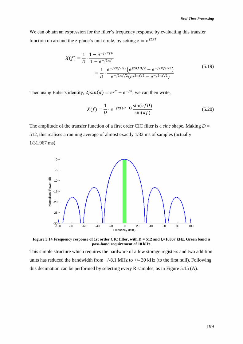
Real-Time Processing
199
We can obtain an expression for the filter’s frequency response by evaluating this transfer
function on around the z-plane’s unit circle, by setting 𝑧 = 𝑒𝑗2𝜋𝑓
𝑋(𝑓) =
1
𝐷∙1 − 𝑒−𝑗2𝜋𝑓𝐷
1 − 𝑒−𝑗2𝜋𝑓
=1
𝐷∙𝑒−𝑗2𝜋𝑓𝐷/2(𝑒𝑗2𝜋𝑓𝐷/2 − 𝑒−𝑗2𝜋𝑓𝐷/2)
𝑒−𝑗2𝜋𝑓/2(𝑒𝑗2𝜋𝑓/2 − 𝑒−𝑗2𝜋𝑓/2)
(5.19)
Then using Euler’s identity, 2𝑗𝑠𝑖𝑛(𝛼) = 𝑒𝑗𝛼 − 𝑒−𝑗𝛼, we can then write,
𝑋(𝑓) =
1
𝐷∙ 𝑒−𝑗𝜋𝑓(𝐷−1)
sin (𝜋𝑓𝐷)
sin (𝜋𝑓) (5.20)
The amplitude of the transfer function of a first order CIC filter is a sinc shape. Making D =
512, this realises a running average of almost exactly 1/32 ms of samples (actually
1/31.967 ms)
Figure 5.14 Frequency response of 1st order CIC filter, with D = 512 and fs=16367 kHz. Green band is
pass-band requirement of 10 kHz.
This simple structure which requires the hardware of a few storage registers and two addition
units has reduced the bandwidth from +/-8.1 MHz to +/- 30 kHz (to the first null). Following
this decimation can be performed by selecting every R samples, as in Figure 5.15 (A).
-100 -80 -60 -40 -20 0 20 40 60 80 100-30
-25
-20
-15
-10
-5
0
Frequency (kHz)
Norm
alis
ed P
ow
er,
dB

200
Figure 5.15 Running average filter followed by decimation(A). Rearrangement to reduce sample rate of
comb section (B)
The decimation can be rearranged to be before the comb stage and therefore reduce the rate
of the comb section and the number of samples stored. This poly-phase filter implementation
is shown in Figure 5.15(B). Following decimation, the frequency response folds over to alias
higher frequency terms into the required pass-band, Figure 5.16. The red regions show where
the high frequency terms will alias into the pass-band. This is then shown folded into the
post-decimation sampled bandwidth in Figure 5.17.
Figure 5.16 The CIC filter response from Figure 5.14, showing the new sampled bandwidth, fs,out/2.
Signal energy in the red bands will then be aliased into the green pass-band.

Real-Time Processing
201
Figure 5.17 Aliasing into the pass-band (green)
There are two undesirable features of the scheme. The first is that there is a sloping
attenuation towards the edge of the pass-band. The second is that there is aliasing of high-
frequency terms into the pass-band
Taking the first issue, the slope in the pass-band, the decimated bandwidth has been kept
wider than the required pass-band, which was defined as -5 kHz to +5 kHz. This allows for
the filter response, so that at the slope by the required region is just 0.35 dB attenuation. As
the attenuation is known, the received power can be scaled in post-processing as an additional
term in the DDM inversion model. Additionally the attenuation being small, the SNR is
minimally affected. The second issue is the aliasing into the pass-band of high frequency
terms. The greatest aliased terms are attenuated by 15 dB by the CIC filter at the edges of the
pass-band. This will introduce some additional noise to the pass-band but as the noise would
be coherently added to the received signal it would slightly increase the variance in the DDM
power measured.
The two undesirable effects are sufficiently small that the onboard DDM processor can use
this scheme to improve the computational complexity.
5.7. DDM Processor Implementation
The DDM processing scheme of Section 5.6.2 has been built into SSTL SGR-ReSI receiver
as part of this project. The following is a description of the realisation of the design used in
the receiver and some results taken from the hardware.
-15 -10 -5 0 5 10 15-60
-50
-40
-30
-20
-10
0
Frequency (kHz)
Norm
alis
ed P
ow
er,
dB
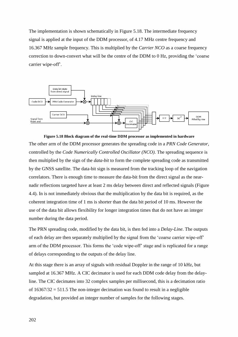
202
The implementation is shown schematically in Figure 5.18. The intermediate frequency
signal is applied at the input of the DDM processor, of 4.17 MHz centre frequency and
16.367 MHz sample frequency. This is multiplied by the Carrier NCO as a coarse frequency
correction to down-convert what will be the centre of the DDM to 0 Hz, providing the ‘coarse
carrier wipe-off’.
Figure 5.18 Block diagram of the real-time DDM processor as implemented in hardware
The other arm of the DDM processor generates the spreading code in a PRN Code Generator,
controlled by the Code Numerically Controlled Oscillator (NCO). The spreading sequence is
then multiplied by the sign of the data-bit to form the complete spreading code as transmitted
by the GNSS satellite. The data-bit sign is measured from the tracking loop of the navigation
correlators. There is enough time to measure the data-bit from the direct signal as the near-
nadir reflections targeted have at least 2 ms delay between direct and reflected signals (Figure
4.4). In is not immediately obvious that the multiplication by the data bit is required, as the
coherent integration time of 1 ms is shorter than the data bit period of 10 ms. However the
use of the data bit allows flexibility for longer integration times that do not have an integer
number during the data period.
The PRN spreading code, modified by the data bit, is then fed into a Delay-Line. The outputs
of each delay are then separately multiplied by the signal from the ‘coarse carrier wipe-off’
arm of the DDM processor. This forms the ‘code wipe-off’ stage and is replicated for a range
of delays corresponding to the outputs of the delay line.
At this stage there is an array of signals with residual Doppler in the range of 10 kHz, but
sampled at 16.367 MHz. A CIC decimator is used for each DDM code delay from the delay-
line. The CIC decimates into 32 complex samples per millisecond, this is a decimation ratio
of 16367/32 = 511.5 The non-integer decimation was found to result in a negligible
degradation, but provided an integer number of samples for the following stages.

Real-Time Processing
203
The result is a group of a complex signals sampled at 32 kHz for each of the delay rows
(240 rows according to our specification in Table 5.3).
The frequency estimation stage is carried out by a hardware implementation of the FFT
algorithm, the hardware resources of which are minimised by implementing one unit and
serially streaming through the samples for each delay channel.
The FFT uses a length of signal, 𝑇𝑐𝑜ℎ= 1 ms, so that 32 data samples are used, which are then
padded by ‘dummy zeros’. An actual FFT of 128 points is used with the remaining 96 points
left zero for a DFT of periodicity 4 ms. This achieves the 250 Hz specification of frequency
resolution and avoids scalloping losses between FFT bins.
The output from the FFT is the coherent accumulation of the DDM for 1 ms. The power of
the complex signal is then found and this is accumulated for a configurable time period from
40 ms up to several seconds. This is the resultant product and is output off to storage
memory, then downlinked through the satellite transmitter to the ground for inversion into
surface roughness measurements.
The approach is a RAM limited design; this means that the FPGA RAM resources provide
the limit to the DDM size and resolution, not the reprogrammable logic resources as was the
case for the time-domain correlator. RAM is utilised by the coherent accumulation store that
buffers the samples for input to the FFT, and the incoherent accumulations that sum the
DDM.
The full system design as implemented in hardware is shown in Appendix D. There is a
considerable degree of extra complexity for control, configuration and self-test purposes over
the functional description given here.
To demonstrate correct operation of the DDM processor in the SGR-ReSI, the processor was
steered to the delay and Doppler of a direct GPS C/A signal. Figure 5.19 shows a single
DDM output from the implementation of the DDM processor. The DDM processor was
configured for 250 Hz Doppler bin spacing, delay spacing of 1 sample of 0.061 μs with 1 ms
coherent integration and incoherent accumulation for 500 ms. A new output DDM is
therefore generated in real-time every 500 ms and stored to the SGR-ReSI internal storage.
This has then been downloaded from the receiver and plotted here.

204
Figure 5.19 A result from real-time DDM output from playback of UK-DMC dataset R44 PRN10 direct
signal and 500 ms integration
Cuts through the DDM are shown as a Doppler map in Figure 5.20(A) and a delay map in
Figure 5.20(B). To verify the performance of the real-time, hardware DDM processor the
output is compared to the map of the same direct GPS C/A signal processed by the software
receiver.
(A) (B)
Figure 5.20 Cuts through the real-time DDM processor output compared to software receive. Data set
R44, PRN10 (A) Doppler map. (B) Delay map
The software receiver processed the DDM without approximation and with floating-point
arithmetic precision. The agreement with the hardware receiver validates this processing
-6000 -4000 -2000 0 2000 4000 60000
0.5
1
1.5
2
2.5
3
x 106
Corr
ela
tion M
agnitude [
arb
.]
Frequency [kHz]
Real-Time Processor
Software Processor
0 1 2 3 4 5 6 70
0.5
1
1.5
2
2.5
3
3.5
x 106
Corr
ela
tion M
agnitude [
arb
.]
Delay [ s]
Real-Time Processor
Software Processor

Real-Time Processing
205
architecture and the FPGA implementation in fixed-point arithmetic. The equivalence of the
two methods shows that the real-time DDM processing implemented in the SGR-ReSI FPGA
successfully processes the DDM with computational complexity reduced sufficiently for real-
time processing.
The direct signal was used for this validation as it provides a high SNR signal and
demonstrates that the DDM processor is functioning correctly, with independence of the
tracking algorithms.
The data rate produced by the DDM processor is, (𝑁𝑑 ∙ 𝑁𝑓 ∙ 𝑁𝑅 ⋅ 𝑁𝑄)/ 𝑇𝑖𝑛𝑐𝑜ℎ bits, which is
respectively the product of the number of delay pixels, Doppler pixels, bits per pixel, number
of reflection channels and the incoherent integration time in seconds. The incoherent
integration time, 𝑇𝑖𝑛𝑐𝑜ℎ, in the DDM processor is configurable on-the-fly, but the nominal
configuration of the processor implemented has specification, 𝑁𝑑 = 128, 𝑁𝑓 = 52, 𝑁𝑅 = 1,
𝑁𝑄 = 10 bits and 𝑇𝑖𝑛𝑐𝑜ℎ = 1 second. This results in a data rate of 65 Kibit/s.
This is a very significant reduction in data from the raw sample downlink of (2 ⋅ 𝑓𝑠 ⋅ 𝑄𝑏) bits
per second, where the nadir and zenith channels are sampled at 𝑓𝑠 Hz and quantised to 𝑄𝑏
bits. For the SGR-ReSI configuration this would be 62 Mibits/s.
5.8. Real-Time Tracking
Onboard processing of the reflected signals is required to reduce the data rate of the output
downlinked to the ground. The DDM processor as described in the previous section will
process a small range of the total delay and Doppler signal space, so it is necessary to track
the reflected signal to keep it centred in the DDM correlation channels.
This section reports on a method of real-time tracking to steer the correlation channels to the
reflection delay and Doppler. The real-time tracking is an extension of the work carried out
on the software receiver described in Chapter 4. The software receiver operated by post-
processing recorded data collections. The real-time receiver has to perform the same
processing but on an embedded processor with limited resources and in hard time limits. In
addition, calculations can no longer be made available ahead of time, as in the post-
processing software receiver, which introduces a further challenge to the implementation.
The tracking geometric or open-loop tracking, means that the predicted specular point is used
alone to steer the correlators, without update from the reflection power measured from the
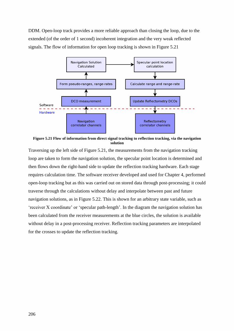
206
DDM. Open-loop track provides a more reliable approach than closing the loop, due to the
extended (of the order of 1 second) incoherent integration and the very weak reflected
signals. The flow of information for open loop tracking is shown in Figure 5.21
Figure 5.21 Flow of information from direct signal tracking to reflection tracking, via the navigation
solution
Traversing up the left side of Figure 5.21, the measurements from the navigation tracking
loop are taken to form the navigation solution, the specular point location is determined and
then flows down the right-hand side to update the reflection tracking hardware. Each stage
requires calculation time. The software receiver developed and used for Chapter 4, performed
open-loop tracking but as this was carried out on stored data through post-processing; it could
traverse through the calculations without delay and interpolate between past and future
navigation solutions, as in Figure 5.22. This is shown for an arbitrary state variable, such as
‘receiver X coordinate’ or ‘specular path-length’. In the diagram the navigation solution has
been calculated from the receiver measurements at the blue circles, the solution is available
without delay in a post-processing receiver. Reflection tracking parameters are interpolated
for the crosses to update the reflection tracking.
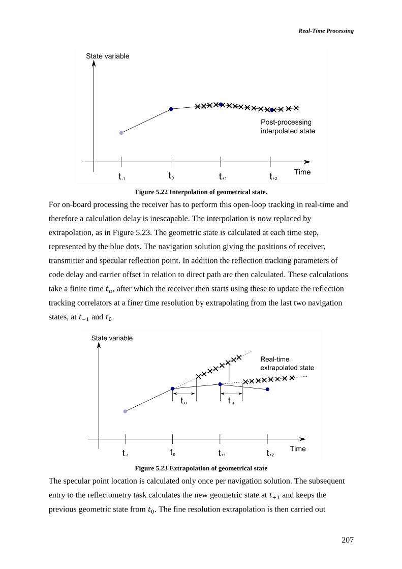
Real-Time Processing
207
Figure 5.22 Interpolation of geometrical state.
For on-board processing the receiver has to perform this open-loop tracking in real-time and
therefore a calculation delay is inescapable. The interpolation is now replaced by
extrapolation, as in Figure 5.23. The geometric state is calculated at each time step,
represented by the blue dots. The navigation solution giving the positions of receiver,
transmitter and specular reflection point. In addition the reflection tracking parameters of
code delay and carrier offset in relation to direct path are then calculated. These calculations
take a finite time 𝑡𝑢, after which the receiver then starts using these to update the reflection
tracking correlators at a finer time resolution by extrapolating from the last two navigation
states, at 𝑡−1 and 𝑡0.
Figure 5.23 Extrapolation of geometrical state
The specular point location is calculated only once per navigation solution. The subsequent
entry to the reflectometry task calculates the new geometric state at 𝑡+1 and keeps the
previous geometric state from 𝑡0. The fine resolution extrapolation is then carried out

208
between these two states. This saves recalculating the time-consuming specular point
calculation unnecessarily.
The fine-grained extrapolation updates the receiver’s DDM correlators with the following
parameters: code phase, code frequency and carrier frequency as with the software receiver.
Due to the accelerating motions of receiver, specular point and transmitter, the extrapolation
introduces an error. So the timing of the measurements up from the navigation hardware, and
back down to the reflectometry hardware has to be carefully handled to reduce the calculation
latency 𝑡𝑢. The allowable latency depends on the accelerations, which are now investigated in
an orbital simulation.
An example tracking log is shown in Figure 5.24 from an orbital simulation with a receiver at
700 km altitude in a circular orbit and GNSS transmitter at 20,200 km altitude. This is an
orbital period of 99 minutes. The simulation is run from when a transmitter appears over the
horizon until it disappears back over the horizon again. The geometry has been chosen so that
at 0 seconds the receiver and specular point are directly below the transmitter.
Figure 5.24 From orbital simulation: Direct and reflected path lengths
The rate of change of the path delay is shown in Figure 5.25. The specular path delay of
(𝑻𝑺𝑹⃗⃗ ⃗⃗ ⃗⃗ ⃗⃗ ), is seen to be stationary at when 𝑻, S and R are aligned and this is when the maximum
acceleration of path delay occurs.
-2000 -1500 -1000 -500 0 500 1000 1500 200065
70
75
80
85
90
95
100
Time [s]
Path
dela
y [
ms]
Path delay (TR)
Path delay (TSR)
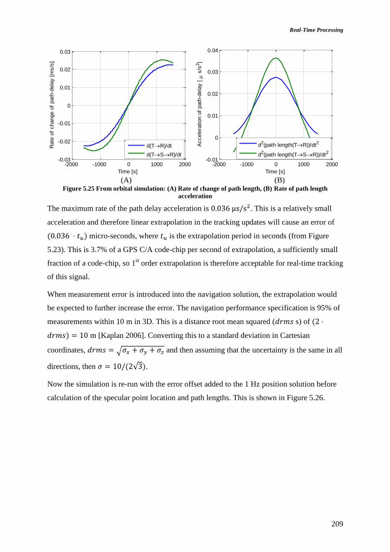
Real-Time Processing
209
(A) (B)
Figure 5.25 From orbital simulation: (A) Rate of change of path length, (B) Rate of path length
acceleration
The maximum rate of the path delay acceleration is 0.036 μs/s2. This is a relatively small
acceleration and therefore linear extrapolation in the tracking updates will cause an error of
(0.036 ⋅ 𝑡𝑢) micro-seconds, where 𝑡𝑢 is the extrapolation period in seconds (from Figure
5.23). This is 3.7% of a GPS C/A code-chip per second of extrapolation, a sufficiently small
fraction of a code-chip, so 1st order extrapolation is therefore acceptable for real-time tracking
of this signal.
When measurement error is introduced into the navigation solution, the extrapolation would
be expected to further increase the error. The navigation performance specification is 95% of
measurements within 10 m in 3D. This is a distance root mean squared (𝑑𝑟𝑚𝑠 s) of (2 ⋅
𝑑𝑟𝑚𝑠) = 10 m [Kaplan 2006]. Converting this to a standard deviation in Cartesian
coordinates, 𝑑𝑟𝑚𝑠 = √𝜎𝑥 + 𝜎𝑦 + 𝜎𝑧 and then assuming that the uncertainty is the same in all
directions, then 𝜎 = 10/(2√3).
Now the simulation is re-run with the error offset added to the 1 Hz position solution before
calculation of the specular point location and path lengths. This is shown in Figure 5.26.
-2000 -1000 0 1000 2000-0.03
-0.02
-0.01
0
0.01
0.02
0.03
Time [s]
Rate
of
change o
f path
-dela
y [
ms/s
]
d(TR)/dt
d(TSR)/dt
-2000 -1000 0 1000 2000-0.01
0
0.01
0.02
0.03
0.04
Time [s]
Accele
ration o
f path
-dela
y [
s
/s2]
d2(path length(TR))/dt2
d2(path length(TSR))/dt2

210
(A) (B)
Figure 5.26 From orbital simulation: (A) Rate of change of path length, (B) Rate of path length
acceleration
The maximum rate of the path delay acceleration is now 0.1 μs/s2. So now extrapolation
whilst waiting for the next tracking update will cause an error of (0.1 ⋅ 𝑡𝑢) micro-seconds,
which is 10% of a GPS C/A code-chip per second of extrapolation. As the SGR-ReSI will be
calculating its navigation solution at 1 Hz, then the extrapolation introduces an error that is
not significant.
5.8.1. Real-Time Tracking Implementation
A basic implementation of the real-time tracking was implemented on the SGR-ReSI receiver
to control the DDM processor. The simultaneous development of the SGR-ReSI’s navigation
functionality at SSTL during the course of this project meant that it was not possible to fully
test the reflectometry real-time tracking. The continuation of the work has been funded by
SSTL to so as to complete the porting of the tracking algorithms developed in this research
into the SGR-ReSI for launch in TDS-1. The following description is of the basic tracking
implementation for controlling the DDM processor and a test methodology to verify the full
real-time receiver on the ground.
The task structure is designed to augment those of the navigation function of the receiver.
This example implementation of real-time GNSS-R tracking is shown as a series of tasks for
which the timing is shown in Figure 5.27. Higher priority tasks are at the bottom of the figure
and interrupt the lower priority tasks above. Time progresses moving to the right of the
diagram and the duration of the tasks is not drawn to scale. The responsibilities of each of the
-2000 -1000 0 1000 2000-0.03
-0.02
-0.01
0
0.01
0.02
0.03
Time [s]
Rate
of
change o
f path
-dela
y [
ms/s
]
d(TR)/dt
d(TSR)/dt
-2000 -1000 0 1000 2000-0.1
-0.05
0
0.05
0.1
0.15
Time [s]
Accele
ration o
f path
-dela
y [
s
/s2]
d2(path length(TR))/dt2
d2(path length(TSR))/dt2
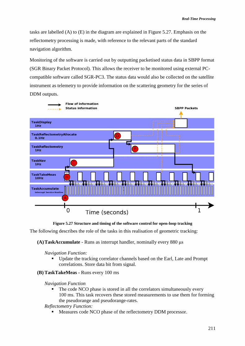
Real-Time Processing
211
tasks are labelled (A) to (E) in the diagram are explained in Figure 5.27. Emphasis on the
reflectometry processing is made, with reference to the relevant parts of the standard
navigation algorithm.
Monitoring of the software is carried out by outputting packetised status data in SBPP format
(SGR Binary Packet Protocol). This allows the receiver to be monitored using external PC-
compatible software called SGR-PC3. The status data would also be collected on the satellite
instrument as telemetry to provide information on the scattering geometry for the series of
DDM outputs.
Figure 5.27 Structure and timing of the software control for open-loop tracking
The following describes the role of the tasks in this realisation of geometric tracking:
(A) TaskAccumulate - Runs as interrupt handler, nominally every 880 μs
Navigation Function:
Update the tracking correlator channels based on the Earl, Late and Prompt
correlations. Store data bit from signal.
(B) TaskTakeMeas - Runs every 100 ms
Navigation Function
The code NCO phase is stored in all the correlators simultaneously every
100 ms. This task recovers these stored measurements to use them for forming
the pseudorange and pseudorange-rates.
Reflectometry Function:
Measures code NCO phase of the reflectometry DDM processor.

212
Extrapolate the range and range rate from the two states stored in the
ReflectionTracking structure and use the extrapolated values to set up the
DDM processor with:
- Code NCO rate
- Carrier NCO rate
- Code NCO phase by slewing code phase.
(C) TaskNav - runs once per second
Navigation Function
Use the code phase measurements from (B) to calculate the navigation
solution: position, velocity and time.
Store the position and velocity of the GPS transmitters
(D) TaskReflectometryAllocate - runs every 10 s
Reflectometry Function:
Calculate the location of reflections from each of the tracked satellites (using
simplified, spherical Earth approximation)
Put these into list and sort list by desirability of the reflections (closest to
antenna boresight or manual selection of PRN number)
(E) TaskReflectometry - runs once per second
Reflectometry Function:
Loop through reflection list, allocating the possible reflections to reflectometry
channels
For each reflection channel:
- Store previous specular point and tracking parameters in
ReflectionTracking structure.
- Calculate the specular point for current navigation solution (from C)
- Calculate the tracking parameters (range and range rate) from
transmitter to specular point to receiver
- Store new tracking parameters in ReflectionTracking structure ready
for task (B)
5.9. Verification and Demonstration
The verification plan is based on demonstrating that the algorithms are working on the SGR-
ReSI by using the in-built data recorder in reverse, which is to playing back the existing data
from the UK-DMC experiment through the receiver. By running real spaceborne data through
the instrument before its launch into orbit, almost every aspect of the system design is tested
including the operation of the real-time DDM co-processor and onboard tracking for
predicting GNSS reflections and the ground software for monitoring and control. The only
exception is the RF link budget that will need to be tested separately before the SGR-ReSI is
launched on TechDemoSat-1.

Real-Time Processing
213
The flow of data for the ground-based verification is shown in Figure 5.28. The same
verification flow can be used for the SGR-ReSI, when in orbit, as that being used for UK-
DMC. The difference being that the UK-DMC raw data files were sampled at a different
sample frequency to the new SGR-ReSI receiver so these are converted using a fractional
sample rate converter and the DC bias removed. UK-DMC would downlink only raw
samples, but the new SGR-ReSI on TDS-1, as a result of this research, will also downlink
processed DDMs and the tracking data that was used during the processing.
Figure 5.28 Schematic of the data flow for the verification of the real-time GNSS-R system
To play back recorded data on the ground, the raw sampled IF data files, need to be
transferred to the on-ground SGR-ReSI’s internal memory. A mechanism was implemented
as part of this work to transfer data into the SGR-ReSI’s inbuilt storage and the data logger
was modified to allow the playback of raw data into the receiver whilst simultaneously
writing processed DDMs back into the memory.
As the UK-DMC data files are just 20 seconds in length and the raw-data logger functionality
of the SGR-ReSI only extends this to 2 minutes, these require a hot-start functionality to
allow the receiver to start navigating in just a few seconds. This was incorporated by SSTL
engineers and was reduced down to around 10 seconds for initialisation. This leaves a further
10 seconds of UK-DMC data per collection available for reflectometry validation before
more is collected following the TDS-1 is launched.
The demonstration of the working GNSS-R receiver required a number of developments in
communication and control for reflectometry processing in the SGR-ReSI. The status packet

214
outputs of the receiver can be seen in Figure 5.29. The reflection specular point locations are
being calculated and are being displayed on a world map. This is occurring in real-time whilst
DDMs are being simultaneously calculated.
Figure 5.29 Monitoring the real-time tracking within SGR-PC3 software
The basic real-time tracking implemented in this research allowed targeting of the direct
signals to verify operation of the DDM processor. In addition the implementation would
calculate the reflection point location, as shown in Figure 5.29, but the steering of the DDM
to the specular reflection remains as part of the SGR-ReSI project’s future work as the
simultaneous development of navigation functionality on the SGR-ReSI at SSTL during the

Real-Time Processing
215
course of this project meant that the full reflectometry real-time tracking could not be
implemented within this research.
The tracking algorithm developed in this thesis has been demonstrated to work in post-
processing with the software receiver and the performance evaluated against the UK-DMC
data sets (Section 4.2). The implementation in real-time processing is not expected to present
any new challenges other than those identified here.
5.10. Real-time Processing Discussion
This chapter has addressed the principal challenge for a satellite based GNSS-R sensor,
reducing the rate of data production to within the downlink capabilities of a small satellite
platform. Before this work the existing approach was to store the full bandwidth of the down-
converted and digitised RF signal. This was seen to be incompatible with continuous
operation of the receiver, so would only allow intermittent operation, like the 20 second
duration data collections on UK-DMC.
A processing approach has been developed that reduces the data-rate significantly through
on-board real-time processing of reflected signal DDMs. The approach reduces the requires
downlink rate for raw signals by a factor of about 1000, depending on configuration which
enabled the receiver to fit within the constraints continuous data rate output less than
500 Kibit/s.
The real-time processing approach combines digital signal processing techniques calculate
the DDM through Doppler spectrum estimation in the frequency domain. The bandwidth is
then reduced by filtering and decimation to reduce the computational complexity. The filter
and decimation stages are optimised to introduce negligible distortion to the DDM. This real-
time processing has been designed into the SGR-ReSI receiver’s coprocessor FPGA and has
been validated on real signals. This is a new development in GNSS-R that processes the
extended signal space over which the reflection is spread in a method that is optimised for
spaceborne GNSS-R.
To target the on-board processing to the location of the reflections a tracking approach has
been developed based on geometric tracking. This was validated on the software receiver of
Chapter 4, by post-processing of UK-DMC data. The extension of geometric tracking to real-
time operation through extrapolation of the tracking parameters has been analysed and a
method proposed for implementation in the GNSS-R receiver. This tracking method has
216
opened the opportunity for on-board processing in a spaceborne receiver by providing a
technique that is suitable to target the DDM processing to the reflections. In addition a test
and validation method has been designed for the ground-based testing of the receiver design
before launch. This allows immediate testing with existing data from UK-DMC and
subsequent to the launch for validation of the processing and to allow updated techniques to
be developed as the DDM inversion techniques are improved.
These real-time DDM processing and real-time tracking developments provide a significant
step towards collecting the validation data required for spaceborne remote sensing of ocean
roughness from GNSS-R. The DDM processing implemented in the SGR-ReSI receiver to be
launched on the TDS-1 satellite specifically progresses this goal of collecting validation data
and the subsequent aim of an operational service providing global coverage and frequent
sampling of the ocean surface.

Discussion and Conclusions
217
Chapter 6: Discussion and Conclusions
Existing satellite remote sensing techniques have typically relied on extensive data sets to
validate satellite measurements with the ground truth. This thesis contributes to the state-of-
the-art by providing a system design for a receiver that can collect the required validation
data set for GNSS-R surface roughness measurement from orbit. The critical parts of the
design were then implemented either in a post-processing software receiver or in a prototype
real-time space GNSS receiver.
This chapter provides a synopsis of the contributions made by this research and then some
suggestions for future work in this area where the research could be extended. Firstly the
contributions are described, which due to the practical emphasis of this work are both
industrial as well as academic.
6.1. Contributions
The contributions made in this research are placed in two areas. The first of which is the
development of techniques for remote sensing of the Earth’s surface using GNSS signals,
these techniques are then extended to the second area which is the design of a receiver for
accommodation on a small satellite.
A system design trade-off for a remote sensing instrument that targets the application of the
ocean roughness determination within the constraints of a small satellite platform is carried
out in Chapter 3. A model of the scattering around the specular point is used to investigate
key aspects of the system design of the GNSS-R receiver. In particular the novel
contributions were the analysis of the new signals in the modernising navigation systems and
their suitability for scatterometric sensing with an antenna design within the constraints of a
satellite platform. According to model, the new wide-band signals such as Galileo E5a/b were
found to need a significantly greater antenna gain to achieve the same RF link budget as the
GPS L1 C/A signals due to the reduced footprint on the Earth’s surface. The increase in
antenna gain for a fixed beam antenna would reduce beam-width resulting in significantly
reduced sensing coverage. The most suitable GNSS signals for a mission with a small scale
antenna are in the bandwidth range of 2 to 4 MHz which included the Galileo E1 signal.
218
The development of a software receiver for post-processing GNSS-R techniques is carried
out in Chapter 4. The software receiver is used to verify the geometric tracking algorithms
that will be needed for real-time processing of reflected signals. New contributions have been
made to the method of calculation of the specular point location. An approximation for a
quasi-spherical Earth was developed that allows deterministic calculation time, suitable for a
real-time implementation. Additionally the method in [Gleason & Gebre-Egziabher 2009]
was improved to allow proper convergence to the solution on an ellipsoidal Earth model.
A new technique for utilising the E1 Galileo signals by combining sub-components was
developed in Section 4.5 and then tested using reflections of the GIOVE-A signals picked up
from orbit. A practical real-time architecture was developed that will allow, future GNSS-R
missions to target Galileo reflections and therefore potentially doubling the coverage over
that of using solely GPS signals.
The Stare processing approach was developed in Section 4.6 for retrieving high-resolution
surface roughness measurements from a GNSS-R receiver. The concept was originally based
on monostatic altimetry techniques first applied to GNSS in [Germain & Ruffini 2002] and
has been examined in detail for the first time here. This method of targeting the signal
processing so that it remains staring at a fixed point on the Earth’s surface as the receiver and
transmitter move, is a promising approach to determine the surface roughness. The novel
contributions made in this research are in determining the sensitivity to ocean surface
roughness, providing a method of correcting for the changing measurement surface area, the
first demonstration on real signals from an orbiting receiver and determining the impact on a
practical receiver implementation.
The software receiver system has allowed the complete set of data collections from UK-DMC
to be processed for the first time. Additionally all specular points are processed to gain a
greater statistical sample. From this a catalogue of the collections has been generated that
enables the full data set to be distributed to other organisations for the first time.
The analysis of the system design and the developments made in the reflection post-
processing addressed the principal challenges for a satellite based GNSS-R sensor: weak
signals, the inversion of receiver measurements into surface parameters and calibration. The
remaining significant challenge identified in the system design was in meeting the data
downlink budget. To overcome this, an on-board processing and real time tracking technique
were developed.

Discussion and Conclusions
219
The real-time DDM processing approach reduces the rate of data produced for downlink by a
factor of about 1000 from that of recording the raw signals as used by UK-DMC’s receiver.
This is a new approach that processes the extended signal space over which the reflection is
spread in a method that is optimised for spaceborne GNSS-R. This real-time processing has
been designed into the SGR-ReSI receiver’s coprocessor FPGA and has been validated on
real signals. To target the DDM processor to the location of the reflections the geometric
tracking approach was developed and tested in the software receiver and it was shown how
this can be extended to real-time tracking.
A ground-based test and validation method has been developed so that as well as in-orbit
processing, logged data can be recorded and post processed using the software receiver or
played through an SGR-ReSI on the ground. These real-time DDM processing and real-time
tracking developments provide a significant step towards collecting the data required for
validation of ocean roughness retrieval by spaceborne GNSS-R remote sensing. The launch
of the receiver developments from this research on the TDS-1 satellite will provide the
opportunity to perform the required model validation and allow progression towards an
operational service for global coverage and frequent sampling of the ocean surface.
6.2. Future Work
As a result of this thesis, a GNSS-R receiver has been designed that is going to be flown on a
forthcoming satellite launch. Following from this the future work spans the areas of operating
the instrument, refinements to the method for inversion of measurement into surface
properties and research into further applications.
The GNSS-R capabilities developed in this project require the support of a careful calibration
and validation campaign where the satellite measurements are compared to truth data from
in-situ measurements or other remote measurements. This stage is expected to include
determination of the inversion method through empirical matching of receiver outputs to the
scattering response. This is expected to be possible as a result of the work carried out in this
thesis.
The DDM on-board processing reduces the data rate for downlink by orders of magnitude
over the previous approaches of full-bandwidth sampling. This means that the receiver will
be able to operate continuously, collecting more validation data and operationally providing
greater sampling coverage. The DDMs have potential for further compression on board the

220
satellite to reduce the downlink rate further. Possible future investigations include the
approach of masking off pixels that correspond to delays that would be above the Earth’s
surface, or parameterisation of the DDM surface by curve fitting.
The work in Stare processing, through modelling the scattering and testing on a real
spaceborne data set has advanced the knowledge on this technique, which has highlighted the
potential for further research into this relatively unexploited approach. Some new areas that
have been opened up by this research are in extending the analysis to investigate the
sensitivity to wave direction and combining Stare processing with the deconvolution
approach of [Bian 2007] to increase resolution.
This work has focused on remote sensing of the ocean surface; a further area of potential
research is in new applications over the cryosphere. The measurement of ice elevation or
indirectly measuring the ionospheric delays in the atmosphere through GNSS-R are
considered to be potential applications. Terrain with significant elevation changes presents a
particular challenge for geo-location of the measurements due to the sensing geometry being
particularly sensitive to altitude. There are a number of avenues that could be considered for
extending measurement to these surfaces.
6.3. Publications and Presentations
The work contained in this thesis has been presented at a number of conferences and
workshops. The following is a list of the presented papers.
Presentations:
P. Jales, M. Unwin, C. Underwood, “Spaceborne Demonstration of Galileo Signals for GNSS
Reflectometry”, Royal institute of Navigation (RIN) New Navigator Conference, London,
2007
P. Jales, M. Unwin, C. Underwood, “Recent Results from UK-DMC Experiment – Ice
Sensing and Reception of Galileo Signals”, GNSS-R 2008 Workshop, ESTEC Noordwijk
Netherlands, September 2008
Papers and presentations:
P. Jales; R. Weiler; M. Unwin, C. Underwood, “First Spaceborne demonstration of Galileo
signals for GNSS Reflectometry”, Institute of Navigation (ION) GNSS Conference,
Savannah Georgia USA, September 2008
R. M. Weiler, P. Blunt, P. Jales, M. Unwin, S. Hodgart, “Performance of an L1/E5 GNSS
Receiver using a Direct Conversion Front-End Architecture”, Institute of Navigation (ION)
GNSS Conference, Savannah Georgia USA, September 2008

Discussion and Conclusions
221
M. Unwin, P.Jales, C. Underwood, “Proposed Satellite Service for Ice-Edge and Storm
Warning Using GNSS Reflectometry”, Royal Institute of Navigation (RIN) NAV08
conference, London, October 2008
R. de Vos van Steenwijk, M. Unwin, P. Jales “Introducing the SGR-ReSI: A Next Generation
Spaceborne GNSS Receiver for Navigation and Remote-Sensing”, NAVITEC, ESA, 2010
(Contributing Author)
P. Jales, “GNSS-Reflectometry: Techniques for Scatterometric Remote Sensing”, Institute of
Navigation GNSS, Portland, Oregon, 2010 (ION GNSS Student Paper Award)
P. Jales, M. Unwin, C. Underwood, “Processing techniques for a GNSS-R scatterometric
remote sensing instrument” GNSS-R 2010, Barcelona, 2010

222
References
Anderson, C., Macklin, T., et al., 2000. Towards a unified theoretical model of ocean
backscatter for wind speed retrieval from SAR, scatterometer and altimeter. CERSAT
News, (11), p.Scientific Topic No. 1.
Bakshi, K.A., Bakshi, A.V. & Bakshi, U.A., 2009. Antennas And Wave Propagation 2009th
ed., Technical Publications Pune.
Barrick, D., 1968. Rough Surface Scattering Based on the Specular Point Theory. Antennas
and Propagation, IEEE Transactions on, 16(4), pp.449– 454.
Bass, F.G. & Fuks, I.M., 1977. Wave scattering from statistically rough surfaces, Oxford;
New York: Pergamon Press.
Bastide, F., Akos, D., et al., 2003. Automatic Gain Control (AGC) as an Interference
Assessment Tool. In ION GPS/GNSS 2003. Portland OR.
Beckmann, P. & Spizzichino, A., 1987. The scattering of electromagnetic waves from rough
surfaces, Norwood, MA: Artech House.
Benedicto, J., Dinwiddy, S.E., et al., 2000. GALILEO: Satellite System Design. European
Space Agency.
Bian, K., 2007. Space-borne Application of GNSS Reflectometry for Global Sea State
Monitoring. PhD Thesis. University of Surrey
Bian, K., Pechev, A. & Mackin, S., 2006. Modelling and data analysis of GPS reflections
from low earth orbit. In Proceedings of SPIE. p. 63600K.
Borre, K., Akos, D., et al., 2006. A Software-Defined GPS and Galileo Receiver: A Single-
Frequency Approach, Birkhauser.
Boyd, S.P. & Vandenberghe, L., 2004. Convex optimization, New York: Cambridge.
Buck, C. & D’Addio, S., 2007. Status and perspectives of GNSS-R at ESA. In Geoscience
and Remote Sensing Symposium, 2007. IGARSS 2007. IEEE International.
Geoscience and Remote Sensing Symposium, 2007. IGARSS 2007. IEEE
International. pp. 5076–5079.
Camps, A., Bosch-Lluis, X., et al., 2007. New Instrument Concepts for Ocean Sensing:
Analysis of the PAU-Radiometer. Geoscience and Remote Sensing, IEEE
Transactions on, 45(10), pp.3180–3192.
Camps, A., Bosch-Lluis, X., et al., 2009. New Passive Instruments Developed for Ocean
Monitoring at the Remote Sensing Lab—Universitat Politècnica de Catalunya.
Sensors, 9(12), pp.10171–10189.

References
223
Caparrini, M., Germain, O., et al., 2003. A system for monitoring a feature of a surface with
broad swath and high resolution.
Cardellach, E., Ruffini, G., et al., 2003. Mediterranean Balloon Experiment: ocean wind
speed sensing from the stratosphere, using GPS reflections. Remote Sensing of
Environment, 88(3), pp.351–362.
Cardellach, E. & Rius, A., 2007. Sea surface slopes’ PDF from GNSS reflected signals. In
Geoscience and Remote Sensing Symposium, 2007. IGARSS 2007. IEEE
International. IEEE, pp. 1342–1345.
Chao, V., Lowe, S., et al., 2011. Prospects of GNSS Reflectometry Science from the ACES
Mission GNSS Receiver onboard the International Space Station. In Workshop on the
Geodesy Applications of ACES Mission. GeoForschungsZentrum Potsdam.
China Satellite Navigation Project Center, 2009. COMPASS/BeiDou Navigation Satellite
System Development. In The 4th Meeting of International Committee on GNSS. Saint
Petersburg Russia.
Clarizia, M.P., Gommenginger, C.P., et al., 2009. Analysis of GNSS-R delay-Doppler maps
from the UK-DMC satellite over the ocean. Geophys. Res. Lett., 36(2), p.L02608.
Clarizia, M.P., Gommenginger, C., et al., 2008. Global navigation satellite system-
reflectometry (GNSS-R) from the UK-DMC satellite for remote sensing of the ocean
surface. In Geoscience and Remote Sensing Symposium, 2008. IGARSS 2008. IEEE
International. IEEE, pp. I–276–I–279.
Clarizia, M.P., Di Bisceglie, M., et al., 2009. Simulation of GNSS-R returns for delay-
DOPPLER analysis of the ocean surface. In Geoscience and Remote Sensing
Symposium, 2009 IEEE International, IGARSS 2009. IEEE, pp. II–182–II–185.
Cox, C. & Munk, W., 1954. Measurement of the roughness of the sea surface from
photographs of the sun’s glitter. J Opt Soc Amer, 44.
Czopek, F.M. & Shollenberger, S., 1993. Description and performance of the GPS Block I
and II L-Band antenna and link budget. In Proceedings of the 6th International
Technical Meeting of the Satellite Division of The Institute of Navigation (ION GPS
1993). pp. 37–43.
D’Addio, S. & Buck, C., 2008. Performance assessment of GNSS-R space based
scatterometry by means of delay-Doppler map. In Geoscience and Remote Sensing
Symposium IGARSS 2008.
ECMWF, 2007. European Centre for Medium-Range Weather Forecasts. Available at:
http://www.ecmwf.int/ [Accessed November 4, 2007].
Elfouhaily, T., Chapron, B., et al., 1997. A unified directional spectrum for long and short
wind-driven waves. Journal of Geophysical Research, 102(C7), pp.15781–15,796.
Elfouhaily, T., Thompson, D.R. & Linstrom, L., 2002. Delay-Doppler analysis of bistatically
reflected signals from the ocean surface: theory and application. IEEE Transactions
on Geoscience and Remote Sensing, 40(3), pp.560–573.

224
ESA, 2008. PARIS In-orbit Demonstrator Dossier.
Esterhuizen, S., Franklin, G., et al., 2009. TriG-A GNSS Precise Orbit and Radio Occultation
Space Receiver.
Evans, D.L., Alpers, W., et al., 2005. Seasat--A 25-year legacy of success. Remote Sensing
of Environment, 94(3), pp.384–404.
Figa-Saldana, J., Wilson, J.J.W., et al., 2002. The advanced scatterometer (ASCAT) on the
meteorological operational (MetOp) platform: A follow on for European wind
scatterometers. Canadian journal of remote sensing, 28(3), pp.404–412.
Fisher, S.C. & Ghassemi, K., 1999. GPS IIF-the next generation. Proceedings of the IEEE,
87(1), pp.24–47.
Fu, L.-L. & Cazenave, A., 2000. Satellite Altimetry and Earth Sciences a Handbook of
Techniques and Applications., Burlington: Elsevier.
Fung, A.K., Zuffada, C. & Hsieh, C.Y., 2001. Incoherent bistatic scattering from the sea
surface at L-band. Geoscience and Remote Sensing, IEEE Transactions on, 39(5),
pp.1006–1012.
Galileo Project Office, 2010. European GNSS (Galileo) Open Service Signal In Space
Interface Control Document.
Galileo Project Office, 2007. GIOVE-A+B Navigation Signal-in-Space Interface Control
Document, ESA-DTEN-NG-ICD/02837.
Garrison, J.L., Komjathy, A., et al., 2002. Wind speed measurement using forward scattered
GPS signals. Geoscience and Remote Sensing, IEEE Transactions on, 40(1), pp.50–
65.
Garrison, J.L. & Katzberg, S.J., 1997. Detection of ocean reflected GPS signals: theory and
experiment. In Southeastcon 97. Engineering New Century., Proceedings. IEEE. pp.
290–294.
Garrison, J.L., Katzberg, S.J. & Hill, M.I., 1998. Effect of sea roughness on bistatically
scattered range coded signals from the Global Positioning System. Geophysical
research letters, 25(13), pp.2257–2260.
Gatti, G., Garutti, A., et al., 2001. The GIOVE-A satellite: from design to in-orbit
commissioning. In Proceedings of the 19th International Technical Meeting of the
Satellite Division of The Institute of Navigation (ION GNSS 2006). pp. 2542–2547.
Germain, O. & Ruffini, G., 2002. Ocean winds and mesoscale topography using GNSS-
PARIS. In Woods Hole meeting.
Gleason, S., 2006. Remote Sensing of Ocean, Ice and Land Surfaces Using Bistatically
Scattered GNSS Signals From Low Earth Orbit. PhD Thesis. University of Surrey.
Gleason, S. & Adjrad, M., 2005. An attempt to sense ocean winds and waves empirically
using bi-static GNSS reflections in low Earth orbit. In Geoscience and Remote

References
225
Sensing Symposium, 2005. IGARSS’05. Proceedings. 2005 IEEE International.
IEEE, pp. 1959–1962.
Gleason, S. & Gebre-Egziabher, D., 2009. GNSS applications and methods, Boston Mass.:
Artech House.
Gleason, S., Gommenginger, C. & Cromwell, D., 2010. Fading statistics and sensing
accuracy of ocean scattered GNSS and altimetry signals. Advances in Space
Research, 46(2), pp.208–220.
Gold, R., 1967. Optimal binary sequences for spread spectrum multiplexing (Corresp.). IEEE
Transactions on Information Theory, 13(4), pp.619–621.
GPS Directorate, 2011. Interface Specification IS-GPS-200F.
Hajj, G., Zuffada, C. & Thomas, J., 2002. Theoretical description of a bistatic system for
ocean altimetry using the GPS signal. IEEE Transactions on Geoscience and Remote
Sensing.
Hall, C. & Cordey, R., 1988. Multistatic scatterometry. In International Geoscience and
Remote Sensing Symposium (IGARSS 1988) on Remote Sensing: Moving Towards
the 21st Century. p. p 561–562.
Helm, A., Beyerle, G., et al., 2007. The Gnss Occultation, Reflectometry, And Scatterometry
Space Receiver Gors: Current Status And Future Plans Within Gitews.
Hodgart, S.M. & Blunt, P.D., 2007. Dual-estimate receiver of Binary Offset Carrier (BOC)
modulated signals for global navigation satellite systems. Electronic Letters, 43(16),
p.877.
Holthuijsen, L.H., 2007. Waves in oceanic and coastal waters, Cambridge: Cambridge
University Press.
IGS, 2010. IGS - International GNSS Service. Available at: http://igscb.jpl.nasa.gov/
[Accessed September 11, 2011].
Jales, P.J., 2010. GNSS-Reflectometry: Techniques for Scatterometric Remote Sensing. In
Proceedings of the 23rd International Technical Meeting of The Satellite Division of
the Institute of Navigation (ION GNSS 2010). pp. 2761–2770.
Jones, W.L., Schroeder, L. & Wentz, F., 1977. Algorithm for inferring wind stress from
SEASAT-A. Satellite applications to marine technology, pp.255–263.
Junered, M., 2007. Enabling hardware technology for GNSS software radio research,
Licentiate thesis, Luleå University of Technology.
Kaplan, E., 2006. Understanding GPS : principles and applications 2nd ed., Boston: Artech
House.
Komjathy, A., Zavorotny, V.U., et al., 2000. GPS Signal Scattering from Sea Surface: Wind
Speed Retrieval Using Experimental Data and Theoretical Model. Remote Sensing of
Environment, 73(2), pp.162–174.

226
Liou, Y.A., 2010. Radio occultation method for remote sensing of the atmosphere and
ionosphere, InTech. Available at: http://www.intechweb.org/books/show/title/radio-
occultation-method-for-remote-sensing-of-the-atmosphere-and-ionosphere [Accessed
May 6, 2012].
Liou, Y.-A., Pavelyev, A.G., et al., 2007. FORMOSAT-3/COSMIC GPS Radio Occultation
Mission: Preliminary Results. Geoscience and Remote Sensing, IEEE Transactions
on, 45(11), pp.3813 –3826.
Liu, T., 2005. El Niño Watch From Space. Available at: http://airsea-
www.jpl.nasa.gov/ENSO/enso.html [Accessed April 23, 2011].
Liu, W., 2002. Progress in Scatterometer Application. Journal of Oceanography, 58(1),
pp.121–136.
Loiselet, M., Stricker, N., et al., 2000. GRAS-Metop’s GPS-based atmospheric sounder. ESA
bulletin, 102, pp.38–44.
Lowe, S.T., LaBrecque, J.L., et al., 2002a. First spaceborne observation of an Earth-reflected
GPS signal. Radio Science, 37(1), p.1007.
Lowe, S.T., LaBrecque, J.L., et al., 2002b. First spaceborne observation of an Earth-reflected
GPS signal. Radio Sci., 37(1), p.1007.
Lyons, R., 2011. Understanding digital signal processing 3rd ed., Upper Saddle River NJ:
Prentice Hall.
Marchan-Hernandez, J.F., Ramos-Perez, I., et al., 2007. PAU-GNSS/R, a real-time GPS-
reflectometer for Earth observation applications: Architecture insights and
preliminary results. In Geoscience and Remote Sensing Symposium, 2007. IGARSS
2007. IEEE International. IEEE, pp. 5113–5116.
Marshall, J. & Plumb, R.A., 2008. Atmosphere, ocean, and climate dynamics: an introductory
text, Elsevier Academic Press.
Martin-Neira, M., 1993. A Passive Reflectometry and Interferometry System(PARIS)-
Application to ocean altimetry. ESA journal, 17(4), pp.331–355.
Martín-Neira, M., D’Addio, S., et al., 2011. The PARIS ocean altimeter in-orbit
demonstrator. Geoscience and Remote Sensing, IEEE Transactions on, (99), pp.1–29.
MathWorks Mapping Toolbox, 2012. Mathworks: Understanding Spherical Coordinates.
Available at: http://www.mathworks.co.uk/help/toolbox/map/ [Accessed April 9,
2012].
Mattos, P.G., 2005. Acquisition of the Galileo OAS L1b/c signal for the mass-market
receiver. In Institute of Navigation (ION GNSS 2005). Long Beach, CA, pp. 1143 –
1152.
Maussang, F., Garello, R., et al., 2011. GPS passive bistatic radar system in oceanic
environment: detection performance estimation. In OCEANS, 2011 IEEE-Spain.
IEEE, pp. 1–5.
References
227
MAXIM, 2007. MAX2769 Universal GPS Receiver Datasheet.
Meehan, T.K., Esterhuizen, S., et al., 2007. TOGA, a prototype for an optimal orbiting
GNSS-R instrument. In International Geoscience & Remote Sensing Symposium.
Misra, P. & Enge, P., 2006. Global positioning system : signals, measurements, and
performance 2nd ed., Lincoln Mass.: Ganga-Jamuna Press.
Mitel, 1997. Datasheet DW9255: SAW Filter for GPS Receivers.
Moore, R.K., Claassen, J.P., et al., 1974. Simultaneous active and passive microwave
response of the earth-The Skylab radscat experiment. In Remote Sensing of
Environment. pp. 189–217.
NOAA, 2012. National Data Buoy Center. Available at: http://www.ndbc.noaa.gov/
[Accessed April 21, 2012].
Nogues-Correig, O., Cardellach Gali, E., et al., 2007. A GPS-reflections receiver that
computes Doppler/delay maps in real time. Geoscience and Remote Sensing, IEEE
Transactions on, 45(1), pp.156–174.
Pany, T., 2010. Navigation signal processing for GNSS software receivers, Norwood MA:
Artech House.
Parmar, R.M., Arora, R.K., et al., 2006. OCEANSAT 2: mission and its applications. In
Proceedings of SPIE. p. 64070C.
Pierson, W.J. & Moskowitz, L., 1964. A proposed spectral form for fully developed wind
seas based on the similarity theory of S.A. Kitaigordskii. Journal of Geophysical
Research, (69), pp.5181–5190.
POGO, 2011. Welcome to POGO. Available at: http://www.ocean-partners.org/ [Accessed
April 23, 2011].
Polischuk, G.M., Kozlov, V.I., et al., 2002. The global navigation satellite system
GLONASS: Development and usage in the 21st century. In 34th Annual Precise Time
and Time Interval (PTTI) Meeting.
Press, W., Teukolsky, S., et al., 1992. Numerical recipes in C (2nd ed.): the art of scientific
computing, Cambridge University Press.
Ribo, S., Arco, J.C., et al., 2007. ASAP, towards a PARIS instrument for space. In
Geoscience and Remote Sensing Symposium, 2007. IGARSS 2007. IEEE
International. IEEE, pp. 2916–2919.
Richards, J.A., 2009. Remote sensing with imaging radar, Berlin; Heidelberg: Springer-
Verlag. Available at: http://www.myilibrary.com?id=245943 [Accessed June 17,
2012].
Rooney, E., Unwin, M., et al., 2007. GIOVE-A In-Orbit Testing Results. In ION GNSS 2006.
Fort Worth, Texas, USA, pp. 25–28.
228
Ruffini, G., Caparrini, M., et al., 2003. Oceanpal: an instrument for remote sensing of the
ocean and other water surfaces using GNSS reflections. Elsevier Oceanography
Series, 69, pp.146–153.
Ruffini, G., Cardellach, E., et al., 1999. Remote sensing of the ocean by bistatic radar
observations: a review, IEEC Rep. WP 1000, ESD-iom 019/99. Earth Sci. Dept,
Radar Group, Barcelona.
Ruffini, G., Soulat, F., et al., 2004. The Eddy Experiment: Accurate GNSS-R ocean altimetry
from low altitude aircraft. Arxiv preprint physics/0406025.
Sagiraju, P.K., Agaian, S. & Akopian, D., 2006. Reduced complexity acquisition of GPS
signals for software embedded applications. Radar, Sonar and Navigation, IEE
Proceedings -, 153(1), pp.69–78.
Sagiraju, P.K., Raju, G.V.S. & Akopian, D., 2008. Fast acquisition implementation for high
sensitivity global positioning systems receivers based on joint and reduced space
search. Radar, Sonar & Navigation, IET, 2(5), pp.376–387.
Sajabi, C., Chen, C.-I.H., et al., 2006. FPGA Frequency Domain Based GPS Coarse
Acquisition Processor Using FFT. In IMTC Instrumentation and Measurement
Technology Conference. Serrento, Italy.
Sarkar, A., Basu, S., et al., 2002. Auto-correlation analysis of ocean surface wind vectors.
Journal of Earth System Science, 111(3), pp.297–303.
Skolnik, M.I. ed., 2008. Radar handbook 3rd ed., New York: McGraw-Hill.
Soulat, F., Caparrini, M., et al., 2004. Sea state monitoring using coastal GNSS-R. Arxiv
preprint physics/0406029.
Soulat, F., 2003. Sea surface remote-sensing with GNSS and sunlight reflections. UPC -
Starlab.
Spaceflight Now, 2009. Spaceflight Now | Breaking News | Wind sensor failure ends long-
lived satellite mission. Available at:
http://spaceflightnow.com/news/n0911/24quikscat/ [Accessed April 23, 2011].
SSTL, 2011. SSTL Space subsystems. Available at: http://www.sstl.co.uk/divisions/systems-
and-services/subsystems [Accessed April 23, 2011].
Stewart, R., 1985. Methods of satellite oceanography, Berkeley: University of California
Press.
Steyn, W.H. & Hashida, Y., 2000. In-orbit attitude and orbit control commissioning of
UoSAT-12. In Spacecraft Guidance, Navigation and Control Systems. p. 95.
Stoffelen, B.A. & Anderson, D., 1997. Ambiguity removal and assimilation of scatterometer
data. Quarterly Journal of the Royal Meteorological Society, 123(538), pp.491–518.

References
229
Thompson, D.R., Elfouhaily, T.M. & Garrison, J.L., 2005. An improved geometrical optics
model for bistatic GPS scattering from the ocean surface. Geoscience and Remote
Sensing, IEEE Transactions on, 43(12), pp.2810–2821.
Tsai, W.T., Spencer, M., et al., 2000. SeaWinds on QuikSCAT: sensor description and
mission overview. In Geoscience and Remote Sensing Symposium, 2000.
Proceedings. IGARSS 2000. IEEE 2000 International. IEEE, pp. 1021–1023 vol. 3.
Tsui, J.B., 2005. Fundamentals of global positioning system receivers: a software approach
2nd ed., New Jersey: John Wiley & Sons, Inc.
Unwin, M., Gleason, S. & Brennan, M., 2003. The Space GPS Reflectometry Experiment On
the UK Disaster Monitoring Constellation Satellite. In ION GPS/GNSS. pp. p2656 –
2663.
Valencia, E., Camps, A., et al., 2010. Advanced architectures for real-time Delay-Doppler
Map GNSS-reflectometers: The GPS reflectometer instrument for PAU (griPAU).
Advances In Space Research, 46(2), pp.196–207.
Voronovich, A.G., 1999. Wave scattering from rough surfaces, Berlin: Springer-Verlag.
De Vos van Steenwijk, R., Unwin, M. & Jales, P., 2010. Introducing the SGR-ReSI: A next
generation spaceborne GNSS receiver for navigation and remote-sensing. In Satellite
Navigation Technologies and European Workshop on GNSS Signals and Signal
Processing (NAVITEC), 2010 5th ESA Workshop on.
Weiler, R., 2009. Investigation of Receiver Architectures and Techniques for Improved
Acquisition and Positioning Performance of new Galileo & GPS Location Signals.
University Of Surrey.
Wentz, F.J., 1991. A Simplified Wind Vector Algorithm for Satellite Scatterometers. Journal
of Atmospheric and Oceanic Technology, 8(5), pp.697–704.
Wikipedia:Geoid, 2011. Geoid. Wikipedia. Available at: http://en.wikipedia.org/wiki/Geoid
[Accessed March 24, 2011].
De Wilde, W., Sleewaegen, J.-M., et al., 2006. Fast signal acquisition technology for new
GPS/Galileo receivers. In Position, Location, And Navigation Symposium, 2006
IEEE/ION. Position, Location, And Navigation Symposium, 2006 IEEE/ION. pp.
1074– 1079.
Willis, N.J., Griffiths, H.D. & Griffiths, H., 2007. Advances in bistatic radar, SciTech
Publishing.
Wu, S., Meehan, T., et al., 1997. The potential use of GPS signals as ocean altimetry
observables. In Proceedings Of The National Technical Meeting-Institute Of
Navigation. Citeseer, pp. 543–550.
Xilinx, 2011. FPGA, CPLD, and EPP Solutions from Xilinx, Inc., Available at:
http://www.xilinx.com/ [Accessed November 19, 2011].
230
Yang, C., 2001. FFT Acquisition of Periodic, Puncture and Overlaid Code Sequences in GPS.
In ION GPS 2001. Salt Lake City, UT.
Zavorotny, V.U. & Voronovich, A.G., 2000. Scattering of GPS signals from the ocean with
wind remote sensing application. Geoscience and Remote Sensing, IEEE Transactions
on, 38(2), pp.951–964.
Zelli, C. & Aerospazio, A., 1999. ENVISAT RA-2 advanced radar altimeter: Instrument
design and pre-launch performance assessment review. Acta astronautica, 44(7-12),
pp.323–333.
Zuffada, C., Fung, A., et al., 2001. The collection of GPS signal scattered off a wind-driven
ocean with a down-looking GPS receiver: polarization properties versus wind speed
and direction. In Geoscience and Remote Sensing Symposium, 2001. IGARSS ’01.
IEEE 2001 International. Geoscience and Remote Sensing Symposium, 2001.
IGARSS ’01. IEEE 2001 International. pp. 3335–3337 vol.7.
Zuffada, C., Elfouhaily, T. & Lowe, S., 2003. Sensitivity analysis of wind vector
measurements from ocean reflected GPS signals. Remote Sensing of Environment,
88(3), pp.341–350.
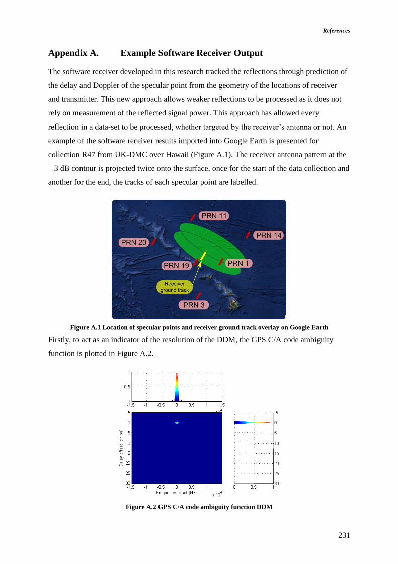
References
231
Appendix A. Example Software Receiver Output
The software receiver developed in this research tracked the reflections through prediction of
the delay and Doppler of the specular point from the geometry of the locations of receiver
and transmitter. This new approach allows weaker reflections to be processed as it does not
rely on measurement of the reflected signal power. This approach has allowed every
reflection in a data-set to be processed, whether targeted by the receiver’s antenna or not. An
example of the software receiver results imported into Google Earth is presented for
collection R47 from UK-DMC over Hawaii (Figure A.1). The receiver antenna pattern at the
– 3 dB contour is projected twice onto the surface, once for the start of the data collection and
another for the end, the tracks of each specular point are labelled.
Figure A.1 Location of specular points and receiver ground track overlay on Google Earth
Firstly, to act as an indicator of the resolution of the DDM, the GPS C/A code ambiguity
function is plotted in Figure A.2.
Figure A.2 GPS C/A code ambiguity function DDM

232
One of the series of DDM for each processed PRN is shown in Figure A.3. These are the
result of 1 ms coherent integrations accumulated for 1 second incoherently. The colour bar
represents the ratio of DDM power to the noise variance. As the maximum power varies
between each DDM, the scale is varied to retain the reflection within the limited dynamic
range of the colour scale; this has the side-effect of making the background noise statistics
appear to vary which is not the case.
Figure A.3 DDMs for UK-DMC data collection R47 for PRNs 1, 3, 11, 20, 14 and 19
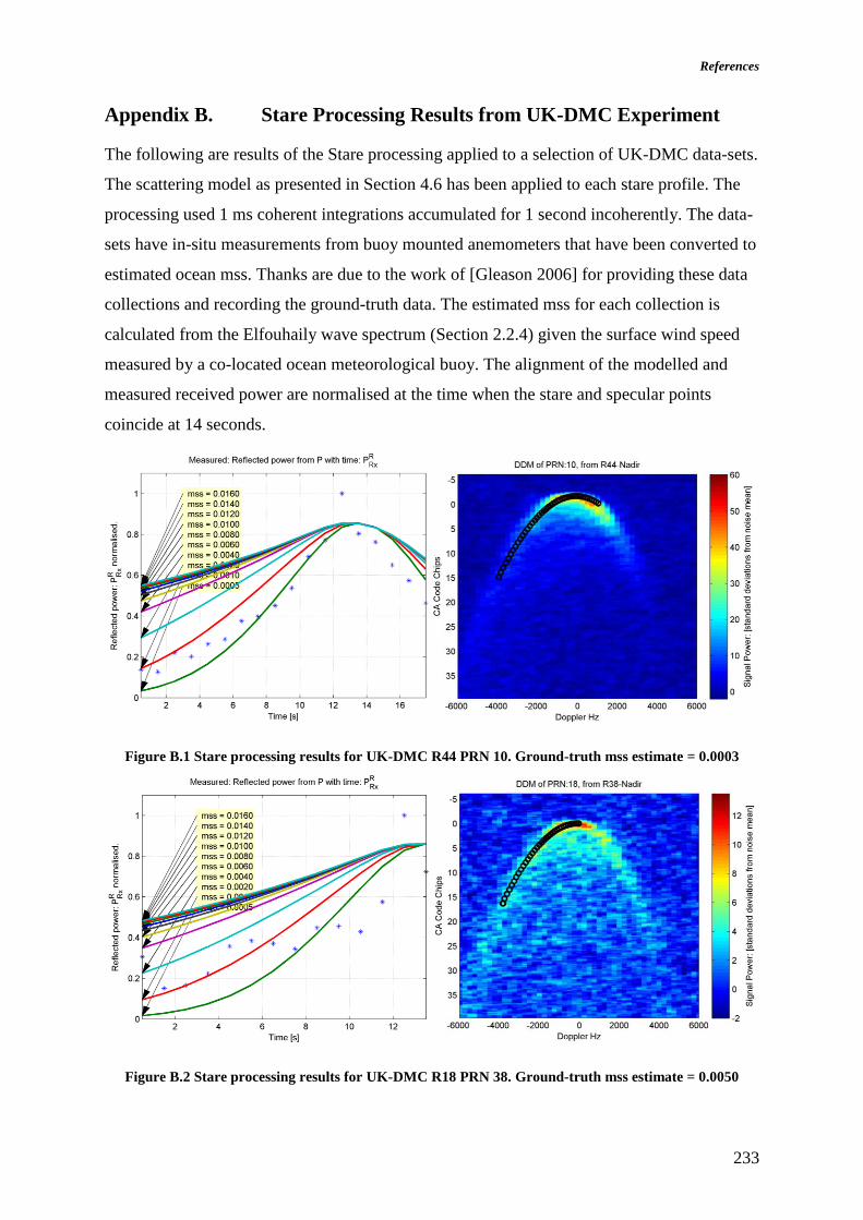
References
233
Appendix B. Stare Processing Results from UK-DMC Experiment
The following are results of the Stare processing applied to a selection of UK-DMC data-sets.
The scattering model as presented in Section 4.6 has been applied to each stare profile. The
processing used 1 ms coherent integrations accumulated for 1 second incoherently. The data-
sets have in-situ measurements from buoy mounted anemometers that have been converted to
estimated ocean mss. Thanks are due to the work of [Gleason 2006] for providing these data
collections and recording the ground-truth data. The estimated mss for each collection is
calculated from the Elfouhaily wave spectrum (Section 2.2.4) given the surface wind speed
measured by a co-located ocean meteorological buoy. The alignment of the modelled and
measured received power are normalised at the time when the stare and specular points
coincide at 14 seconds.
Figure B.1 Stare processing results for UK-DMC R44 PRN 10. Ground-truth mss estimate = 0.0003
Figure B.2 Stare processing results for UK-DMC R18 PRN 38. Ground-truth mss estimate = 0.0050

234
Figure B.3 Stare processing results for UK-DMC R22 PRN 28. Ground-truth mss estimate = 0.0094
Figure B.4 Stare processing results for UK-DMC R10 PRN 17. Ground-truth mss estimate = 0.0164
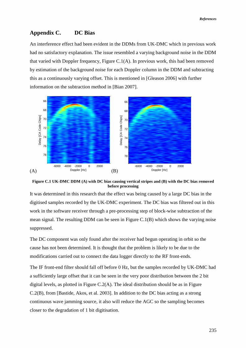
References
235
Appendix C. DC Bias
An interference effect had been evident in the DDMs from UK-DMC which in previous work
had no satisfactory explanation. The issue resembled a varying background noise in the DDM
that varied with Doppler frequency, Figure C.1(A). In previous work, this had been removed
by estimation of the background noise for each Doppler column in the DDM and subtracting
this as a continuously varying offset. This is mentioned in [Gleason 2006] with further
information on the subtraction method in [Bian 2007].
(A) (B)
Figure C.1 UK-DMC DDM (A) with DC bias causing vertical stripes and (B) with the DC bias removed
before processing
It was determined in this research that the effect was being caused by a large DC bias in the
digitised samples recorded by the UK-DMC experiment. The DC bias was filtered out in this
work in the software receiver through a pre-processing step of block-wise subtraction of the
mean signal. The resulting DDM can be seen in Figure C.1(B) which shows the varying noise
suppressed.
The DC component was only found after the receiver had begun operating in orbit so the
cause has not been determined. It is thought that the problem is likely to be due to the
modifications carried out to connect the data logger directly to the RF front-ends.
The IF front-end filter should fall off before 0 Hz, but the samples recorded by UK-DMC had
a sufficiently large offset that it can be seen in the very poor distribution between the 2 bit
digital levels, as plotted in Figure C.2(A). The ideal distribution should be as in Figure
C.2(B), from [Bastide, Akos, et al. 2003]. In addition to the DC bias acting as a strong
continuous wave jamming source, it also will reduce the AGC so the sampling becomes
closer to the degradation of 1 bit digitisation.
Dela
y [
CA
Code C
hip
s]
Doppler [Hz]
Nadir04112007-0058
-6000 -4000 -2000 0 2000
66
68
70
72
74
76
78
Dela
y [
CA
Code C
hip
s]
Doppler [Hz]
Nadir04112007-0058
-6000 -4000 -2000 0 2000
66
68
70
72
74
76
78
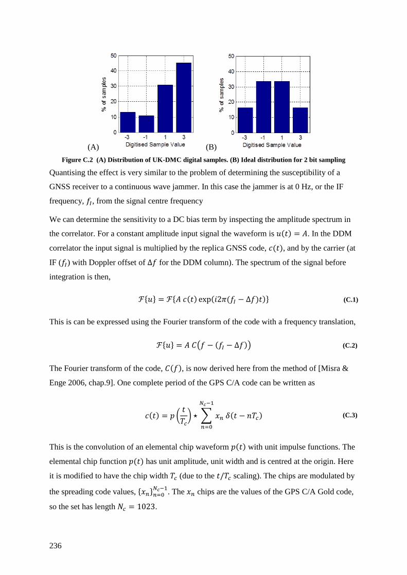
236
(A) (B)
Figure C.2 (A) Distribution of UK-DMC digital samples. (B) Ideal distribution for 2 bit sampling
Quantising the effect is very similar to the problem of determining the susceptibility of a
GNSS receiver to a continuous wave jammer. In this case the jammer is at 0 Hz, or the IF
frequency, 𝑓𝐼, from the signal centre frequency
We can determine the sensitivity to a DC bias term by inspecting the amplitude spectrum in
the correlator. For a constant amplitude input signal the waveform is 𝑢(𝑡) = 𝐴. In the DDM
correlator the input signal is multiplied by the replica GNSS code, 𝑐(𝑡), and by the carrier (at
IF (𝑓𝐼) with Doppler offset of Δ𝑓 for the DDM column). The spectrum of the signal before
integration is then,
ℱ{𝑢} = ℱ{𝐴 𝑐(𝑡) exp(𝑖2𝜋(𝑓𝐼 − Δ𝑓)𝑡)} (C.1)
This is can be expressed using the Fourier transform of the code with a frequency translation,
ℱ{𝑢} = 𝐴 𝐶(𝑓 − (𝑓𝐼 − Δ𝑓)) (C.2)
The Fourier transform of the code, 𝐶(𝑓), is now derived here from the method of [Misra &
Enge 2006, chap.9]. One complete period of the GPS C/A code can be written as
𝑐(𝑡) = 𝑝 (𝑡
𝑇𝑐) ⋆ ∑ 𝑥𝑛 𝛿(𝑡 − 𝑛𝑇𝑐)
𝑁𝑐−1
𝑛=0
(C.3)
This is the convolution of an elemental chip waveform 𝑝(𝑡) with unit impulse functions. The
elemental chip function 𝑝(𝑡) has unit amplitude, unit width and is centred at the origin. Here
it is modified to have the chip width 𝑇𝑐 (due to the 𝑡/𝑇𝑐 scaling). The chips are modulated by
the spreading code values, {𝑥𝑛}𝑛=0𝑁𝑐−1
. The 𝑥𝑛 chips are the values of the GPS C/A Gold code,
so the set has length 𝑁𝑐 = 1023.
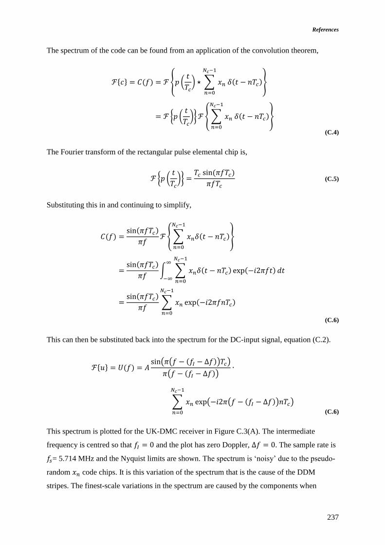
References
237
The spectrum of the code can be found from an application of the convolution theorem,
ℱ{𝑐} = 𝐶(𝑓) = ℱ {𝑝 (𝑡
𝑇𝑐) ⋆ ∑ 𝑥𝑛 𝛿(𝑡 − 𝑛𝑇𝑐)
𝑁𝑐−1
𝑛=0
}
= ℱ {𝑝 (𝑡
𝑇𝑐)} ℱ { ∑ 𝑥𝑛 𝛿(𝑡 − 𝑛𝑇𝑐)
𝑁𝑐−1
𝑛=0
}
(C.4)
The Fourier transform of the rectangular pulse elemental chip is,
ℱ {𝑝 (
𝑡
𝑇𝑐)} =
𝑇𝑐 sin (𝜋𝑓𝑇𝑐)
𝜋𝑓𝑇𝑐 (C.5)
Substituting this in and continuing to simplify,
𝐶(𝑓) =sin(𝜋𝑓𝑇𝑐)
𝜋𝑓ℱ { ∑ 𝑥𝑛𝛿(𝑡 − 𝑛𝑇𝑐)
𝑁𝑐−1
𝑛=0
}
=sin(𝜋𝑓𝑇𝑐)
𝜋𝑓∫ ∑ 𝑥𝑛𝛿(𝑡 − 𝑛𝑇𝑐) exp(−𝑖2𝜋𝑓𝑡)
𝑁𝑐−1
𝑛=0
∞
−∞
𝑑𝑡
=sin(𝜋𝑓𝑇𝑐)
𝜋𝑓∑ 𝑥𝑛 exp(−𝑖2𝜋𝑓𝑛𝑇𝑐)
𝑁𝑐−1
𝑛=0
(C.6)
This can then be substituted back into the spectrum for the DC-input signal, equation (C.2).
ℱ{𝑢} = 𝑈(𝑓) = 𝐴
sin(𝜋(𝑓 − (𝑓𝐼 − Δ𝑓))𝑇𝑐)
𝜋(𝑓 − (𝑓𝐼 − Δ𝑓))∙
∑ 𝑥𝑛 exp(−𝑖2𝜋(𝑓 − (𝑓𝐼 − Δ𝑓))𝑛𝑇𝑐)
𝑁𝑐−1
𝑛=0
(C.6)
This spectrum is plotted for the UK-DMC receiver in Figure C.3(A). The intermediate
frequency is centred so that 𝑓𝐼 = 0 and the plot has zero Doppler, Δ𝑓 = 0. The sample rate is
𝑓𝑠= 5.714 MHz and the Nyquist limits are shown. The spectrum is ‘noisy’ due to the pseudo-
random 𝑥𝑛 code chips. It is this variation of the spectrum that is the cause of the DDM
stripes. The finest-scale variations in the spectrum are caused by the components when

238
𝑛 = 𝑁𝑐 − 1 = 1022. The chip rate is 𝑇𝑐 = 1/(1.023 MHz), so these components modulate
the spectrum at 1 kHz. This characteristic spacing is evident in the DDM in Figure C.1(A).
The ‘sinc’ scaling of the spectrum indicates that the leakage of the DC power into the DDM
can be reduced by moving the IF further from DC.
Figure C.3 Power spectral density of 1W GPS C/A code. (A) Zarlink Nyquist sampling limits. (B) SGR-
ReSI Nyquist sampling limits.
The radio front-end used on UK-DMC (Zarlink) had a relatively low sampling frequency in
comparison to the bandwidth of the GPS C/A code. This results in the Nyquist sampling
limits being relatively close to the centre Intermediate Frequency (IF). This is visible in the
spectrum of the GPS C/A code in Figure C.3(A), which shows that the GPS C/A code 1st side
lobe almost exactly coincides with 0 Hz of the Nyquist sampling limits. This makes it
particularly susceptible to a DC bias as the correlation will only attenuate these components
by −13 dB.
The DC-bias problem has been resolved for the SGR-ReSI in Figure C.3(B) which uses a
faster sample rate and the IF is set so that the spectral null of the GPS signal lies close to
0 Hz, (IF = 4.17 MHz and 𝑓𝑠= 16.367 MHz). The correlation with the GPS signal will then
attenuate any components at 0 Hz down to less than -30 dB of the main lobe without the need
for additional filtering. In addition the SGR-ReSI hardware is being monitored for DC bias to
reduce likelihood of a similar interference affecting the AGC.

References
239
Appendix D. DDM Processor Implementation
The schematic of the DDM processor implementation is shown in Figure D.1.
Figure D.1 DDM correlator system architecture as implemented in the SGR-ReSI co-processor FPGA

240
Appendix E. Catalogue of UK-DMC data collections
Part of the catalogue of UK-DMC collections is reproduced in this appendix. Each row of the
following table corresponds to a specular point’s track over the Earth’s surface. A single data
collection will typically have several specular points within the antenna beam and only these
reflections with a detectable SNR are reported, this is defined here as the peak to RMS noise
power, Γ ≥ 4.5.
The following data fields are shown:
Data Collection Reference: Unique identification of the data collection
Date and Start Time (UTC). The time of the processing initiation, which corresponds to the
first GPS sub-frame in the recorded data.
Surface: Type of surface at start of the specular point’s track (O = Ocean, L = Land) Note
that some of the data-sets were over seasonal sea-ice which would be marked ‘O’.
PRN: identifying number of the GPS transmitter
SP Latitude and Longitude: Position of the specular point at start of the track.
Rx To SP Az and Rx To SP El: The azimuth and elevation angles of the specular point from
the receiver at the start of the track. An azimuth of 0𝑜 is defined as the velocity direction of
the receiver and elevation is defined as −90𝑜 for nadir. Expressed in degrees.
Surface Incidence: The angle between the incident ray and the surface normal for the start of
the track, expressed in degrees.
Antenna Gain: The antenna gain in the direction of the specular point, expressed in units of
dBi.
Specular Point Power SNR: The measure of the ratio of signal to noise power as defined in
Equation (2.32), for the specular path.
Specular Point Detectability: The measure of the signal to noise ratio as defined in Equation
(2.33), which is the peak power to RMS noise ratio for the specular path.

Dat
a C
olle
ctio
n
Re
fere
nce
Dat
e
Star
t Ti
me
(U
TC)
Surf
ace
PR
N
SP L
atit
ud
e
[De
gree
s]
SP L
on
gitu
de
[De
gree
s]
Rx
To
SP
Az
[De
gree
s]
Rx
To
SP
El
[De
gree
s]
Surf
ace
inci
den
ce
[De
gree
s]
An
ten
na
gain
[dB
i]
Spec
ula
r P
oin
t
Po
wer
SN
R
Spec
ula
r P
oin
t
De
tect
abili
ty
R109 02/04/2010 07:55:38 O 3 -44.0 20.4 24.0 -60.5 -33.3 8.4 1.4 9.4
R108 06/02/2010 08:08:38 O 1 -68.8 39.7 81.3 -64.0 -29.3 11.1 1.5 12.6
R108 06/02/2010 08:08:38 O 31 -68.6 26.3 -22.3 -65.0 -28.2 9.6 1.3 8.0
R107 04/02/2010 08:32:32 O 31 -69.0 23.7 -3.6 -70.5 -21.9 10.6 4.2 75.1
R107 04/02/2010 08:32:32 O 29 -65.5 47.9 90.8 -37.4 -62.3 7.3 1.4 9.1
R106 26/01/2010 07:52:44 O 30 -67.3 42.9 59.8 -57.8 -36.5 10.6 24.2 459.8
R106 26/01/2010 07:52:44 O 14 -68.2 37.5 30.2 -67.3 -25.5 10.5 3.4 51.5
R106 26/01/2010 07:52:44 O 26 -66.6 43.8 59.4 -53.0 -42.1 10.0 1.8 15.3
R106 26/01/2010 07:52:44 O 1 -66.4 41.8 49.8 -53.8 -41.2 9.2 1.6 13.1
R106 26/01/2010 07:52:44 O 31 -66.5 21.3 -34.2 -44.0 -53.3 1.6 1.2 6.2
R104 18/02/2009 05:51:20 O 29 11.8 52.3 27.1 -51.2 -44.0 4.6 1.6 12.3
RP04 12/01/2008 15:42:09 O 25 -77.1 -38.3 35.8 -61.1 -32.5 9.6 2.8 48.5
RP04 12/01/2008 15:42:09 L 10 -81.9 -65.5 -65.0 -51.9 -43.3 9.5 1.7 16.2
RAus 05/01/2006 13:39:39 L 9 -30.1 122.9 157.3 -79.1 -12.3 11.7 3.1 7.9
RAus 05/01/2006 13:39:39 L 2 -30.6 127.4 -112.3 -59.6 -34.2 11.1 20.8 427.1
R57 21/12/2005 10:26:10 O 23 58.3 -167.9 -78.4 -78.6 -12.8 10.5 1.3 6.3
R57 21/12/2005 10:26:10 O 20 56.8 -161.5 -86.8 -52.3 -42.8 9.3 1.3 7.9
R56 09/12/2005 20:41:58 O 5 54.8 -172.3 -95.0 -73.9 -18.0 11.2 1.4 10.2
R56 09/12/2005 20:41:58 O 9 53.3 -166.5 158.0 -66.6 -26.3 10.0 1.5 10.6
R56 09/12/2005 20:41:58 O 30 53.5 -178.5 -90.7 -49.2 -46.6 9.4 1.3 7.4
R52 24/11/2005 21:09:04 O 9 51.2 -172.9 128.4 -80.2 -11.0 11.7 1.5 12.0
R52 24/11/2005 21:09:04 O 5 50.3 -178.5 -100.6 -65.8 -27.2 11.3 2.2 28.8
R52 24/11/2005 21:09:04 O 30 47.9 175.7 -101.1 -42.5 -55.0 9.1 1.4 9.6
R51 23/11/2005 10:59:40 O 20 57.1 -176.6 -104.5 -77.4 -14.0 11.4 1.4 8.3
R51 23/11/2005 10:59:40 L 4 59.5 169.8 99.5 -46.8 -49.5 8.7 2.3 23.9
R51 23/11/2005 10:59:40 O 1 61.6 -167.6 -148.4 -42.9 -54.4 0.2 1.4 10.8
R50 21/11/2005 20:55:52 O 9 54.5 -172.6 -138.1 -87.9 -2.5 11.4 1.4 10.1
R50 21/11/2005 20:55:52 O 7 56.1 -164.0 86.3 -52.3 -42.7 8.5 1.2 5.3
R50 21/11/2005 20:55:52 O 30 48.5 174.3 -105.2 -35.0 -65.5 7.7 1.2 4.7
R50 21/11/2005 20:55:52 O 18 49.3 172.9 -98.5 -34.7 -66.0 7.6 1.2 4.6
R49 19/11/2005 10:09:28 O 1 53.3 -163.0 -124.7 -60.7 -32.9 10.8 1.6 14.0
R49 19/11/2005 10:09:28 O 24 54.4 -176.9 101.4 -50.8 -44.5 9.5 1.3 7.1
R49 19/11/2005 10:09:28 O 17 54.6 -177.5 102.1 -49.1 -46.6 9.2 1.3 6.2
R48 18/11/2005 20:41:46 L 7 54.5 -161.2 103.6 -55.5 -38.9 10.2 1.3 6.0
R48 18/11/2005 20:41:46 O 5 50.5 -177.5 -107.9 -45.0 -51.8 9.4 1.5 10.4
R48 18/11/2005 20:41:46 O 17 55.5 -160.5 91.5 -53.1 -41.8 9.2 1.3 6.1
R48 18/11/2005 20:41:46 O 18 51.7 177.2 -86.6 -38.1 -60.9 7.0 1.2 5.1
R48 18/11/2005 20:41:46 O 24 55.6 -145.9 92.3 -30.8 -72.4 3.6 2.5 34.1
R47 12/11/2005 09:11:28 O 1 24.7 -158.6 -101.7 -70.4 -21.9 11.4 1.5 10.4
R47 12/11/2005 09:11:28 O 11 28.6 -164.0 133.7 -54.0 -40.6 8.4 1.3 6.9
R46 24/10/2005 03:51:16 O 10 30.1 -80.6 152.8 -78.3 -12.8 11.7 1.6 14.1
R46 24/10/2005 03:51:16 O 2 31.5 -76.4 -141.9 -57.0 -37.0 8.7 1.5 10.0
R46 24/10/2005 03:51:16 O 4 30.0 -69.5 -111.9 -36.8 -62.6 7.6 1.4 9.1
R45 23/10/2005 04:54:46 O 29 19.1 -93.6 -93.9 -58.6 -35.3 10.6 1.3 6.2
241

Dat
a C
olle
ctio
n
Re
fere
nce
Dat
e
Star
t Ti
me
(U
TC)
Surf
ace
PR
N
SP L
atit
ud
e
[De
gree
s]
SP L
on
gitu
de
[De
gree
s]
Rx
To
SP
Az
[De
gree
s]
Rx
To
SP
El
[De
gree
s]
Surf
ace
inci
den
ce
[De
gree
s]
An
ten
na
gain
[dB
i]
Spec
ula
r P
oin
t
Po
wer
SN
R
Spec
ula
r P
oin
t
De
tect
abili
ty
R45 23/10/2005 04:54:46 O 2 22.3 -87.6 -119.1 -36.2 -63.4 6.5 1.3 6.1
R44 22/10/2005 04:15:16 O 10 29.0 -85.9 -176.9 -70.4 -180.0 10.6 5.4 100.0
R44 22/10/2005 04:15:16 O 2 29.6 -81.1 -133.4 -49.9 -45.5 7.8 3.0 42.0
R44 22/10/2005 04:15:16 L 6 31.7 -91.7 125.8 -45.3 -51.2 7.1 1.4 7.0
R43 07/10/2005 07:52:22 O 15 55.2 -135.3 67.2 -78.2 -13.2 9.9 1.3 6.2
R43 07/10/2005 07:52:22 O 3 57.9 -142.6 103.2 -48.2 -47.6 9.1 1.7 14.1
R43 07/10/2005 07:52:22 L 29 58.9 -122.2 -142.0 -43.8 -53.0 3.4 1.2 4.8
R42 04/10/2005 09:15:10 L 18 61.1 -144.6 -112.4 -64.4 -28.6 11.4 4.1 71.7
R42 04/10/2005 09:15:10 L 15 60.4 -144.9 -99.9 -64.8 -28.2 11.2 25.5 460.2
R42 04/10/2005 09:15:10 L 19 62.2 -159.4 90.6 -56.1 -38.1 9.5 6.4 107.5
R42 04/10/2005 09:15:10 L 21 59.8 -134.9 -106.7 -40.3 -57.7 8.6 1.3 6.1
R40 26/09/2005 09:21:10 O 22 23.0 -162.0 -126.9 -74.1 -17.6 11.6 2.7 38.6
R40 26/09/2005 09:21:10 O 3 26.1 -165.7 142.7 -56.6 -37.4 8.2 2.4 33.4
R40 26/09/2005 09:21:10 O 19 28.7 -170.7 124.8 -37.6 -61.3 4.5 1.2 4.9
R40 26/09/2005 09:21:10 O 18 26.7 -159.2 -149.8 -47.3 -48.6 3.0 1.2 4.8
R38 13/09/2005 09:24:46 O 16 26.1 -166.0 90.5 -73.2 -18.6 10.9 1.3 6.5
R38 13/09/2005 09:24:46 O 18 26.9 -160.3 -123.9 -60.4 -33.1 10.8 1.6 12.4
R38 13/09/2005 09:24:46 O 3 30.3 -168.8 126.0 -46.2 -49.9 7.3 1.3 6.8
R38 13/09/2005 09:24:46 O 22 23.7 -162.4 -49.0 -68.2 -24.4 3.6 1.2 4.5
R37 02/09/2005 08:56:58 L 16 58.1 -155.2 85.0 -58.7 -35.2 9.2 1.2 6.2
R37 02/09/2005 08:56:58 O 3 59.5 -167.9 92.2 -34.4 -66.2 4.8 1.2 4.5
R36 12/08/2005 09:07:28 O 21 18.5 -161.2 140.2 -84.6 -5.9 11.6 1.6 13.6
R36 12/08/2005 09:07:28 O 25 19.2 -166.6 91.1 -49.5 -46.0 8.6 1.8 16.2
R35 10/08/2005 07:46:10 O 30 41.0 -137.6 106.9 -79.4 -11.6 11.4 2.0 25.2
R35 10/08/2005 07:46:10 O 2 43.2 -131.4 -142.7 -54.4 -40.1 7.8 1.5 11.7
R35 10/08/2005 07:46:10 O 21 32.4 -142.9 22.3 -36.2 -63.5 0.4 1.4 9.3
R33 24/07/2005 08:44:40 O 5 15.5 -152.1 -129.5 -57.2 -36.9 10.0 1.7 15.8
R33 24/07/2005 08:44:40 O 6 17.1 -158.8 129.1 -55.3 -39.0 9.1 1.4 8.0
R31 07/07/2005 09:33:34 O 5 23.6 -162.1 -129.3 -52.6 -42.3 9.1 1.5 11.6
R31 07/07/2005 09:33:34 O 30 25.2 -166.5 172.8 -58.9 -34.8 6.7 1.2 4.7
R31 07/07/2005 09:33:34 O 1 26.6 -177.1 108.7 -34.3 -66.3 5.3 1.3 6.1
R30 24/06/2005 09:28:58 O 5 52.8 -156.2 -93.0 -79.6 -11.6 11.1 1.5 12.3
R30 24/06/2005 09:28:58 O 30 53.5 -162.6 85.3 -66.0 -26.8 10.0 1.3 7.5
R30 24/06/2005 09:28:58 O 1 58.4 -169.3 118.4 -39.6 -58.6 6.2 1.7 15.2
R30 24/06/2005 09:28:58 O 4 56.4 -147.8 -139.4 -44.5 -52.2 4.6 1.5 12.0
R26 04/06/2005 10:05:22 O 5 54.2 -166.6 -3.4 -89.4 -0.8 11.0 1.5 14.2
R26 04/06/2005 10:05:22 O 14 55.6 -175.6 92.2 -50.1 -45.3 8.8 1.8 21.4
R26 04/06/2005 10:05:22 O 4 55.5 -153.9 -121.4 -41.9 -55.5 7.6 1.4 9.6
R25 03/06/2005 06:29:22 O 7 -10.4 -126.1 163.7 -66.4 -26.4 9.8 1.6 12.5
R25 03/06/2005 06:29:22 O 24 -14.5 -120.3 -87.7 -49.4 -46.1 9.0 1.3 7.4
R22 17/05/2005 08:50:34 O 26 17.4 -157.8 121.2 -78.3 -12.9 11.6 1.6 13.3
R21 02/05/2005 09:16:04 O 29 23.8 -162.2 167.7 -85.2 -5.2 11.7 1.6 16.0
R21 02/05/2005 09:16:04 O 26 25.0 -163.0 143.0 -72.8 -19.0 11.4 2.9 41.8
R21 02/05/2005 09:16:04 O 9 27.8 -169.7 112.5 -39.5 -58.6 6.7 1.4 8.9
242

Dat
a C
olle
ctio
n
Re
fere
nce
Dat
e
Star
t Ti
me
(U
TC)
Surf
ace
PR
N
SP L
atit
ud
e
[De
gree
s]
SP L
on
gitu
de
[De
gree
s]
Rx
To
SP
Az
[De
gree
s]
Rx
To
SP
El
[De
gree
s]
Surf
ace
inci
den
ce
[De
gree
s]
An
ten
na
gain
[dB
i]
Spec
ula
r P
oin
t
Po
wer
SN
R
Spec
ula
r P
oin
t
De
tect
abili
ty
R21 02/05/2005 09:16:04 O 5 19.6 -169.7 51.8 -40.2 -57.7 3.0 1.2 5.0
R20 21/03/2005 07:29:52 O 13 42.3 -131.0 -159.2 -78.2 -13.0 11.7 1.7 15.9
R20 21/03/2005 07:29:52 O 23 40.6 -127.1 -96.7 -59.7 -34.0 10.8 1.4 8.6
R20 21/03/2005 07:29:52 L 3 39.5 -118.4 -99.1 -34.7 -65.8 7.7 1.2 4.9
R19 11/03/2005 07:46:04 O 13 48.6 -134.2 166.5 -82.3 -8.3 11.8 1.6 11.1
R19 11/03/2005 07:46:04 O 23 47.4 -129.8 -99.8 -64.6 -28.4 11.2 1.9 18.3
R19 11/03/2005 07:46:04 O 2 51.4 -147.7 102.9 -36.7 -62.7 6.2 1.2 5.3
R18 04/03/2005 08:27:10 O 4 15.4 -156.9 73.9 -49.6 -46.0 4.9 1.2 4.7
R16Ice 04/02/2005 10:24:04 O 13 59.0 -162.9 -111.6 -63.2 -30.0 11.3 43.3 644.4
R16Ice 04/02/2005 10:24:04 L 23 58.8 -154.6 -113.1 -41.8 -55.7 8.6 1.2 4.6
R15 30/01/2005 09:05:22 O 20 20.6 -155.4 -114.8 -53.9 -40.6 10.4 2.1 25.8
R15 30/01/2005 09:05:22 O 24 22.5 -163.8 118.4 -54.6 -39.8 9.8 1.5 12.5
R15 30/01/2005 09:05:22 O 13 23.1 -161.9 143.0 -58.7 -35.0 8.8 1.5 11.4
R15 30/01/2005 09:05:22 O 4 24.2 -165.2 122.4 -44.9 -51.5 7.4 1.2 4.6
R13 26/11/2004 07:35:58 O 22 45.7 -131.5 -155.7 -76.7 -14.7 11.6 2.2 29.9
R13 26/11/2004 07:35:58 O 15 44.5 -129.8 -104.3 -71.5 -20.6 11.5 1.8 17.0
R13 26/11/2004 07:35:58 O 19 46.2 -138.5 100.2 -56.1 -38.2 10.1 1.3 7.4
R13 26/11/2004 07:35:58 O 18 47.2 -126.2 -136.4 -50.9 -44.3 7.7 1.4 9.9
R12 16/11/2004 07:54:40 O 22 41.0 -137.9 -165.7 -77.9 -13.3 11.7 1.6 12.6
R12 16/11/2004 07:54:40 O 15 41.1 -136.4 -139.9 -71.1 -20.9 11.3 1.6 12.9
R12 16/11/2004 07:54:40 O 19 42.9 -144.1 114.8 -51.9 -43.1 9.5 1.3 5.7
R12 16/11/2004 07:54:40 O 21 38.8 -128.8 -99.0 -41.1 -56.7 8.8 1.3 6.5
R12 16/11/2004 07:54:40 O 18 43.1 -133.5 -144.7 -51.9 -43.1 6.6 1.3 5.0
R10 03/09/2004 07:25:10 O 30 36.1 -133.6 99.0 -80.9 -10.0 11.2 1.4 8.8
R10 03/09/2004 07:25:10 O 17 37.3 -130.4 -145.5 -70.3 -21.8 11.1 1.6 11.7
R10 03/09/2004 07:25:10 O 6 38.0 -136.9 110.1 -56.6 -37.5 10.3 1.4 10.1
R8 13/07/2004 09:18:22 O 17 14.6 -159.7 -101.5 -53.1 -41.8 10.5 1.3 5.7
R8 13/07/2004 09:18:22 O 14 17.7 -172.3 100.6 -40.8 -57.1 7.3 1.2 5.1
R8 13/07/2004 09:18:22 O 5 19.4 -162.5 -168.6 -51.9 -43.1 2.2 1.2 5.7
R7 09/07/2004 08:34:04 O 6 -14.5 -162.7 80.7 -54.4 -40.2 7.9 1.2 5.3
R6 03/06/2004 08:50:34 O 26 2.2 -160.3 158.1 -74.3 -17.4 11.4 1.8 18.9
R6 03/06/2004 08:50:34 O 5 2.3 -166.6 93.8 -43.7 -53.2 7.6 1.3 7.7
R5 24/05/2004 09:02:52 O 29 16.5 -160.6 -154.6 -87.7 -2.5 11.4 1.3 7.4
R5 24/05/2004 09:02:52 O 7 18.1 -156.7 -128.0 -55.7 -38.6 9.8 1.4 8.7
R4 21/05/2004 08:46:46 O 29 22.2 -156.6 136.0 -80.2 -10.8 11.7 1.9 19.4
R4 21/05/2004 08:46:46 O 26 23.2 -157.2 136.7 -69.9 -22.2 11.2 2.0 19.6
R4 21/05/2004 08:46:46 O 7 21.0 -152.6 -98.6 -63.0 -30.2 11.1 1.4 9.6
R4 21/05/2004 08:46:46 O 8 23.1 -146.5 -116.0 -37.5 -61.4 7.3 1.3 7.3
R3 06/04/2004 08:32:34 O 28 -14.8 -157.6 -163.2 -81.3 -9.7 11.8 1.7 14.8
R3 06/04/2004 08:32:34 O 24 -13.5 -165.5 92.9 -42.3 -55.2 7.2 1.3 7.5
R3 06/04/2004 08:32:34 O 7 -20.3 -158.3 -10.8 -54.2 -40.4 5.5 1.5 10.8
243