Sovereign Risk Premia ∗

Nicola Borri

LUISS

Adrien Verdelhan

MIT Sloan & NBER

December 2010

Abstract

Emerging countries tend to default when their economic conditions worsen. If bad times in an

emerging country correspond to bad times for the US investor, then foreign sovereign bonds are

particularly risky. We explore how this mechanism plays out in the data and in a general equilibrium

model of optimal borrowing and default. Empirically, the higher the correlation between past foreign

and US bond returns, the higher the average sovereign excess returns. In the model, sovereign

defaults and bond prices depend not only on the borrowers’ economic conditions, but also on the

lenders’ time-varying risk-aversion.

∗Borri: Department of Economics, LUISS University, Viale Romania 32, 00197 Rome, Italy; nborri@luiss.it;

Tel: +39 06 85225959; http://docenti.luiss.it/borri/. Verdelhan: Department of Finance, MIT Sloan School of

Management, E62-621, 77 Massachusetts Avenue, Cambridge, MA 02139, and NBER; adrienv@mit.edu; Tel: (617) 253-

5123; http://web.mit.edu/adrienv/www/. The authors thank Cristina Arellano, Marianne Baxter, Charles Engel, Gita

Gopinath, Francois Gourio, Guido Lorenzoni, Hanno Lustig, Jun Pan, Monika Piazzesi, Martin Schneider, Ken Singleton,

Frank Warnock, Vivian Yue, and participants at many conferences and seminars. All remaining errors are our own.

1

In this paper, we study sovereign bonds issued by emerging countries in US dollars and take the

perspective of US investors. We show both empirically and theoretically that covariances between

bond returns and risk factors are key determinants of sovereign bond prices and debt quantities. In

the data, average sovereign bond excess returns line up with their quantities of risk, as implied by

a simple no-arbitrage condition. Building on this finding, we develop a general equilibrium model

of optimal borrowing and lending with endogenous default choices and risk-averse investors. Our

model replicates our asset pricing results. Sovereign risk premia imply a novel link across countries:

lenders’ time-varying risk-aversion influences borrowers’ default decisions, and thus sovereign bond

prices. Opening up capital markets thus exposes emerging countries to US business cycle risk.

The intuition behind our results is simple. US investors are risk-averse and invest in foreign

government bonds. Emerging countries tend to default in ’bad times’, when, for example, their

consumption is low. If bad times in the foreign economy correspond to bad times in the domestic

economy, then foreign countries tend to default in bad times for US investors. In this case, sovereign

bonds are particularly risky, and US investors expect to be compensated for that risk through a high

return. Alternatively, if bad times in the foreign economy correspond to good times for US investors,

then sovereign bonds are less risky and may even hedge US aggregate risk. As a result, sovereign

bond prices depend on both expected probabilities of default and the timing of the bond payoffs.

Risk-aversion implies that optimal borrowing and default decisions depend not only on the borrow-

ers’ but also on the lenders’ economic conditions. Let us assume that business cycles are positively

correlated across countries. In this case, sovereign bonds command positive risk premia. If lenders

are very risk-averse, risk premia are high and interest rates too. In this case, borrowing is not very

attractive and emerging countries might not fear much the exclusion from financial markets that

sovereign defaults entail. As a result, emerging countries choose to default when they experience

bad shocks. The same economic conditions in the borrowing countries, however, would not trigger

defaults if lenders were less risk averse and risk premia lower.

With this price mechanism in mind, we turn to the data on sovereign debt. We look at bonds

issued by emerging countries that are included in JP Morgan’s EMBI Global index. We build portfolios

of sovereign bonds by sorting countries along two dimensions: their default probabilities and their

covariance with US economic conditions. For the first dimension, we use Standard and Poor’s credit

ratings to measure the probability of sovereign default. Credit ratings are not investor-specific and do

not account for the timing of a potential default. For the second dimension, we compute bond betas,

which are defined as the slope coefficients in regressions of one-month sovereign bond excess returns

on one-month US corporate bond excess returns at daily frequency. US corporate bond returns proxy

for domestic economic conditions. Our intuition starts off the correlation between macroeconomic

conditions in emerging countries and in the US, but most emerging countries lack high frequency

macroeconomic data. To address this issue, we thus turn to bonds returns. After sorting countries

along these two dimensions, we obtain six portfolios and a large cross-section of holding period excess

2

returns. Our sample starts in January 1995 and ends in May 2009. If investors were risk-neutral, all

average excess returns should be zero. They are clearly not. The spread in average excess returns

between low and high default probability countries is about 5 percent per year. The spread in average

excess returns between low and high bond beta countries is also about 5 percent per year.

We study this cross-section of excess returns from the perspective of a US investor. We find

that a large fraction of the cross-section of average EMBI excess returns can be explained by their

covariances with just one risk factor: the return on a US BBB corporate bond. Portfolios with higher

exposure to this risk factor are riskier and have higher average excess returns because they offer lower

returns when US corporate default risks are higher, e.g in bad times for the US. The market price

of risk is in line with the mean of the risk factor, as implied by a no-arbitrage condition. Pricing

errors are not statistically significant. Looking at the time-variation in the market price of risk, we

find that it increases in bad times, as measured by a high value of the equity option-implied volatility

(VIX) index. We consider several robustness checks, using different sorting variables and risk factors.

Notably, we obtain similar results when sorting countries on their stock market betas (obtained as slope

coefficients of daily emerging bond excess returns on US stock market returns). Again, our sorting

procedure delivers a clear cross-section of average excess returns and the no-arbitrage condition is

satisfied. All our findings point towards a risk-based explanation of sovereign bond returns.

To uncover the implications of our findings in terms of optimal borrowing, we build on the seminal

work by Eaton and Gersovitz (1981) and use a dynamic general equilibrium model of sovereign lending

and borrowing with endogenous default choice in incomplete markets. In the model, a set of small

open economies borrow from a large developed country (the US). We consider endowment economies.

The only source of heterogeneity across small open economies is their correlation with the US business

cycle. We introduce a key modification to the literature: we assume that investors are risk-averse and

have external habit preferences as in Campbell and Cochrane (1999).

The rest of the model builds on Aguiar and Gopinath (2006) and Arellano (2008). As in the latter

paper, we assume a nonlinear cost of default. As in the former, we assume that foreign endowments

present a time-varying long-run mean. Unlike these papers, we consider simultaneously shocks to the

transitory and permanent components of endowment growth rates. Every period, foreign countries

decide to either default and face exclusion from financial markets, or repay their debt and consider

borrowing again.

The key novelty of the model appears in the link between lenders’ risk premia and borrowers’ optimal

default decisions. In our model, defaults depend partly on lenders’ risk aversion. To illustrate this

point, let us again assume that business cycles are positively correlated. In this case, sovereign bonds

are risky. When lenders experience a series of bad consumption growth shocks, their consumption

becomes closer to their subsistence level and their risk-aversion increase. If lenders are very risk averse,

risk premia are high and interest rates too. Since it is very costly to borrow, emerging countries tend

to default as soon as they experience adverse conditions. As a result, when shocks across countries

3

are positively correlated, defaults in emerging countries are more likely when lenders’ risk aversion is

high. In times of extreme risk-aversion, it looks as if lenders are pushing borrowers to default.

As lenders’ risk aversion influences borrowers’ default decisions, it also impacts optimal debt quan-

tities and prices. Let us again assume that shocks across countries are positively correlated. Sovereign

bonds are then risky investments since borrowers are more likely to default in bad times for investors.

Higher probabilities of default imply higher yields and lower bond prices. Those lower prices occur in

bad times for investors. In equilibrium, these bonds thus offer higher expected returns than bonds

issued by countries whose shocks are not correlated to the lenders’ business cycle. The larger the

risk-aversion, the larger the sovereign risk premium, and the higher the spreads in average excess

returns across countries. As a result, the model offers a general equilibrium view of debt quantities

and prices in which risk premia link lenders’ and borrowers’ economies.

Our model delivers endogenously both high debt levels – as in Aguiar and Gopinath (2006) – and

large bond yields – as in Arellano (2008). In the model, countries borrow heavily, mostly to smooth out

changes in the permanent component of their endowment growth rates. Default probabilities increase

when the permanent components of endowment growth decrease – i.e in bad times. Countries default

after receiving negative (often temporary) shocks. This risk of default is thus compensated by large

spreads, which increase when the emerging country experiences a long period of low growth. As a

result, bond prices reflect the interaction between transitory and permanent shocks. The model, as

its predecessors, matches important features of the emerging markets business cycles.

In order to analyze the model’s results and compare them with actual data, we replicate on

simulated series our previous experiment. The model delivers time-varying equity excess returns in the

US, so we rank countries on stock market betas as we did on actual data and we build portfolios of

simulated sovereign bonds. The model delivers a cross-section of average excess returns. Countries

that are risky from the lenders’ perspective offer higher returns. But bond issuances and defaults are

endogenous choices: countries facing high borrowing costs choose to borrow less, thereby lowering

their default probabilities. In the simulations, high beta countries pay higher interest rates even if

they borrow less in equilibrium. From the perspective of the US investor, the riskiest country is not

the most indebted one, but the one that might default in bad times. We run on simulated data the

same asset pricing tests as on actual data. Since we do not have long term corporate bonds in our

model, we use the simulated US stock market return as our risk factor. As expected, it accounts for

the cross-section of sovereign bond returns. High sovereign excess returns correspond to high beta

portfolios.

The model suggests new approaches to some old puzzling questions. We do not attempt to solve

these puzzles here but simply mention the model’s implications. First, the model implies that there

is no linear relation between interest rates and debt levels, or between interest rates and output.

Second, the model offers an interpretation to the large increase in yields in the fall of 2008, based on

an endogenously higher risk-aversion and thus higher market prices of risk. Finally, the model implies

4

that currency unions might lead to higher borrowing costs since they imply higher business cycles’

synchronizations.

Three discrepancies between the model and the data are worth mentioning. First, average excess

returns and spreads between high and low default probability countries and between high and low beta

countries are smaller than in the data. This discrepancy is likely due to the short maturity of simulated

bonds: we only consider one-period (i.e three-month) bonds, whereas the average maturity is close

to 10 years in the data. Such a maturity difference matters: term structures of credit default swaps

(CDS) rates are strongly upward-sloping on average, with 10-year rates being on average 5 times higher

than short-term rates. As a result, we do not attempt to match actual returns with our one-period

bonds. The model could be extended in this direction: Hatchondo and Martinez (2009) and Chatterjee

and Eyigungor (2010) offer potential mechanisms to increase maturities without adding state variables.

Second, the model does not take into account interest rate risk. Building macroeconomic models of

the yield curve is still a challenge even for closed economies without default risk. This challenge is

particularly obvious for emerging economies because their counter-cyclical real interest rates lead to

downward sloping real yield curves in existing macroeconomic models. We thus leave the extension to

rich yield curve dynamics out for future research. Third, in the model, the cross-country correlation

of endowment shocks is the sole source of heterogeneity across countries. It is constant, while

there is time-variation in the bond betas that we measure. This assumption appears to us as a

natural first step. Adding volatility in these correlations would not add much to the economics of

the model, which already produces some time-variation in betas because of the time-varying means

of endowment growth rates and time-varying risk-aversion. Likewise, adding heterogeneity in the

endowment volatilities would offer a second source of cross-sectional variation in excess returns – and

thus justify sorting countries along two dimensions – but it would not change the mechanism of the

model.

This paper is related to two strands of existing literature on sovereign debt. First, this paper

contributes to the large body of empirical literature on emerging market bond spreads. The paper

closest to ours is Longstaff, Pan, Pedersen and Singleton (2011). They study changes in emerging

market CDS spreads and find that global factors, like the return on the U.S. stock market and changes

in the VIX index, explain a large fraction of the common variation in CDS spreads. They argue

convincingly that CDS are mostly compensation for bearing global risk, with little country-specific

risk premia.1 Second, our paper contributes to the theoretical literature on sovereign lending with

defaults.2 Here, the papers closest to ours are Aguiar and Gopinath (2006) and Arellano (2008). But

1Other references on the empirical determinants of sovereign spreads include papers by Edwards (1984), Boehmer

and Megginson (1990), Adler and Qi (2003), Bekaert, Harvey and Lundblad (2007), Favero, Pagano and von Thadden

(2010), and Hilscher and Nosbusch (2010). See Almeida and Philippon (2007) for related evidence on corporate bond

spreads and its implications on corporate capital structure.2Recent papers in this segment of the literature include Bulow and Rogoff (1989), Atkeson (1991), Kehoe and

Levine (1993), Zame (1993), Cole and Kehoe (2000), Alvarez and Jermann (2000), Duffie, Pedersen and Singleton

(2003), Bolton and Jeanne (2007), Amador (2008), Fostel and Geanakoplos (2008), Arellano and Ramanarayanan (2009),

5

these papers, as many others in the literature, focus on risk-neutral investors. As a result, expected

excess returns are there equal to zero, whereas we uncover large excess returns in the data. A limited

number of papers introduce risk aversion to bear on this topic. Arellano (2008) mostly focus on risk-

neutral investors, but also considers a reduced form of the lenders’ stochastic discount factor that

is similar to constant relative risk-aversion. Lizarazo (2010) investigates decreasing absolute risk-

aversion in the same model. Andrade (2009) specifies an exogenous pricing kernel. Pan and Singleton

(2008) study the term structure of CDS sovereign spreads. Broner, Lorenzoni and Schmukler (2008)

propose a three-period model to determine the optimal term structure of sovereign debt when investors

are risk-averse.

This paper also builds on the macro-finance literature. Without risk-aversion, i.e when investors

are risk-neutral, there is no role for covariances in sovereign bond prices, and expected excess returns

are zero. With constant risk-aversion, the large spread in returns due to covariances would imply a

very large risk-aversion coefficient and an implausible risk-free rate, as Mehra and Prescott (1985) and

Weil (1989) find on equity markets. Campbell and Cochrane (1999) preferences offer a solution to the

equity premium puzzle, endogenously delivering a volatile stochastic discount factor that implies high

Sharpe ratios. Moreover, these preferences entail time-varying risk aversion, and thus a time-variation

in the market price of risk, as in the data.3

The paper is organized as follows. Section 1 describes the data, our empirical methodology, and

our portfolios of sovereign bonds. Section 2 shows that one risk factor explains most of the cross-

sectional variation in average excess returns across our portfolios. In section 3, we interpret these

findings in a general equilibrium model of sovereign borrowing. Section 4 presents a calibrated version

of the model that qualitatively replicates our empirical findings. Section 5 concludes. A separate

appendix reports additional results. Our portfolios of sovereign bond excess returns are available on

our websites, along with the Matlab code to simulate our model.

1 The Cross-Section of EMBI Returns

We take the perspective of a US investor who borrows in US dollars to invest in sovereign bonds

issued in US dollars by emerging countries. We start by describing the raw data and setting up some

notation. Then we turn to our portfolio-building methodology, and report the main characteristics of

our cross-section of sovereign excess returns.

Benjamin and Wright (2009), Pouzo (2009), Chien and Lustig (2010), Yue (2010), and Broner, Martin and Ventura

(2010).3There are at least two other classes of dynamic asset pricing models that account for several asset pricing puzzles: the

long-run risk framework of Bansal and Yaron (2004) and the disaster risk framework of Rietz (1988) and Barro (2006).

These two classes of models deliver volatile stochastic discount factors and high risk premia too. They are legitimate

candidates to describe the representative investor in models of sovereign lending.

6

1.1 Data and notation

Data on Emerging Markets JP Morgan publishes country-specific indices that market partici-

pants consider as benchmarks. The JP Morgan EMBI Global indices cover low or middle income per

capita countries and our main dataset thus contains 36 countries: Argentina, Belize, Brazil, Bulgaria,

Chile, China, Colombia, Cote D’Ivoire, Dominican Republic, Ecuador, Egypt, El Salvador, Hungary,

Indonesia, Iraq, Kazakhstan, Lebanon, Malaysia, Mexico, Morocco, Pakistan, Panama, Peru, Philip-

pine, Poland, Russia, Serbia, South Africa, Thailand, Trinidad and Tobago, Tunisia, Turkey, Ukraine,

Uruguay, Venezuela, Vietnam. The sample period runs from December 1993 to May 2009.

The JP Morgan EMBI Global total return index includes accrued dividends and cash payments.

In each country, the index is a market capitalization-weighted aggregate of US dollar-denominated

Brady Bonds, Eurobonds, traded loans and local market debt instruments issued by sovereign and

quasi-sovereign entities. These bonds are liquid debt instruments that are actively traded. Their

notional sizes are at least equal to $500 million. Each issue included in the EMBI Global index must

have at least 2.5 years until maturity when it enters the index and at least 1 year until maturity to

remain in the index. Moreover, JP Morgan sets liquidity criteria such as easily accessible and verifiable

daily prices either from an inter-dealer broker or a certified JP Morgan source.

To assess the default probability of each country, we rely on Standard and Poor’s credit ratings.

They take the form of letter grades ranging from AAA (highest credit worthiness) to SD (selective

default). They are available for a large set of countries over a long time period. We collect Standard

and Poor’s ratings for all the 36 countries in the EMBI index, except Cote d’Ivoire and Iraq. We focus

on ratings for long-term debt denominated in foreign currencies and convert ratings into numbers

ranging from 1 (highest credit worthiness) to 23 (lowest credit worthiness). Our sample contains

several default episodes. Argentina, the Dominican Republic, Ecuador, Russia and Uruguay defaulted

on their external debt during our sample period. Argentina was in default status from November 2001

to May 2005, the Dominican Republic from February 2005 to May 2005, Ecuador in July 2000 for

only one month, Russia from January 1999 to November 2000, and Uruguay in May 2003 for only

one month.

Ratings are not traded prices. This obvious fact has two consequences. First, ratings are not

tailored to a particular investor. For example, they are the same for a US and a Japanese investor. As

a result, ratings do not not take into account the timing of a potential sovereign default: a country

that might default in good times for the US has the same rating as a country that might default in bad

times. Second, for most countries, credit ratings do not encompass all the information on expected

defaults. They are not updated on a regular basis, but rather when new information or events suggest

the need for additional Standard and Poor’s studies and grade revisions.

To complement the Standard and Poor’s ratings, it is now common to rely on credit default swaps

(CDS) and debt to GNP ratios. These two measures do not seem optimal for our study. CDS are

insurance contracts against the event that a sovereign defaults on its debt over a given horizon. These

7

contracts are traded in US dollars. As a result, their prices reflect both the magnitude and the timing

of expected defaults. More crucially, CDS data are only available from December 2002 on, and for

a small subset of the EMBI Global countries (see Pan and Singleton (2008) for a study of three

countries over the 2001-2006 period). Debt to GNP ratios are available for many countries, but at

annual frequency. These ratios do not predict default probabilities and returns as well than Standard

and Poor’s ratings. To check, however, that high debt levels do not drive our results, we report debt

to GNP ratios. Our series come from the World Bank Global Development Finance annual data set.

We linearly interpolate the annual debt to GNP ratios to obtain monthly series. Appendix A reports

summary statistics on sovereign spreads and debt levels.

Notation Before turning to our portfolio-building strategy, we introduce here some useful notation.

Let r e,i denote the log excess return of an American investor who borrows funds in US dollars at the

risk free rate r f in order to buy country i ’s EMBI bond, then sells this bond after one month, and

pays back her debt. Her log excess return is equal to:

r e,it+1 = pit+1 − pit − r ft ,

where pit denotes the log market price of an EMBI bond in country i at date t. We define the bond

beta (β iEMBI) of each country i as the slope coefficient in a regression of EMBI bond excess returns

on US BBB-rated corporate bond excess returns:

r e,it+1 = αi + β iEMBIre,BBBt + εt ,

where r e,BBBt denotes the log total excess return on the Merrill Lynch US BBB corporate bond index.4

We obtain similar results when we use EMBI and US BBB returns instead of excess returns. We

compute betas on 200-day rolling windows to obtain time-series of β iEMBI,t . As a timing convention,

we date t the beta estimated with returns up to date t. For each regression, we estimate betas only if

at least 50 observations for both the left- and right-hand side variables are available over the previous

200-day rolling window period.

1.2 Portfolios of Excess Returns

EMBI portfolios We build portfolios of EMBI excess returns by sorting countries along two dimen-

sions: their probabilities of defaults and their bond betas. First, at the end of each period t, we sort

all countries in the sample in two groups on the basis of their bond betas βEMBI,t . The first group

contains the countries with the lowest βEMBI,t , the second group contains the countries with the

4We do not attempt here to summarize the large literature on corporate spreads. See Giesecke, Longstaff, Schaefer

and Strebulaev (2010) for a survey and long historical time-series, see Gilchrist, Yankov and Zakrajsek (2009) for recent

evidence, and see Bhamra, Kuehn and Strebulaev (2010) for a recent model with counter-cyclical corporate spreads.

8

highest βEMBI,t . Second, we sort all countries within each of the two groups in three portfolios ranked

from low to high probabilities of default. We measure default probabilities with Standard and Poor’s

credit ratings. As a result, we obtain six portfolios. Portfolios 1, 2 and 3 contain countries with the

lowest betas, while portfolios 4, 5 and 6 contain countries with the highest betas. Portfolios 1 and

4 contain countries with the lowest default probabilities, while portfolios 3 and 6 contain countries

with the highest default probabilities. Portfolios are re-balanced at the end of every month, using

information available at that point. To give an example, Mexico turns out to be a high beta country

on average, while Thailand is a rather low beta country. This is not very surprising considering the

strong connection between the US and Mexican economies. Note, however, that the composition of

portfolios changes every month: Table 11 in Appendix B presents the frequency of reallocation across

portfolios and Figure 5 focuses on the portfolio allocation of Argentina and Mexico.

We compute the EMBI excess returns r e,jt+1 for portfolio j by taking the average of the EMBI

excess returns between t and t + 1 that are in portfolio j . Daily historical levels of the EMBI indices

are available from December 31, 1993 onwards for a limited set of countries. We need at least six

countries in the sample to start building our six portfolios and thus start in January 1995. The size

of our sample varies over time, reaching a maximum of 32 countries.

Table 1 provides an overview of our six EMBI portfolios. For each portfolio j , we report the

average foreign bond beta βjEMBI, the average Standard and Poor’s credit rating, the average total

excess return r e,j , and the average external debt to GNP ratio. All returns are reported in US dollars

and the moments are annualized: we multiply the means of monthly returns by 12 and standard

deviations by√

12. The Sharpe ratio is the ratio of the annualized mean to the annualized standard

deviation.

Our portfolios highlight two simple empirical facts. First, excess returns increase from low to high

betas: portfolio 1, 2 and 3 (low betas) offer lower excess returns than portfolios 4, 5 and 6 (high

betas). The average excess return on all the low beta portfolios is 505 basis points per annum. For

the high beta portfolios, it is 1020 basis points. As a result, there is on average a 500 basis points

difference between high and low beta portfolios. Bilateral comparisons (portfolio 1 versus portfolio

4, 2 versus 5, and 3 versus 6) all show that, for similar credit ratings, high beta bonds always offer

higher returns. Second, excess returns also increase with default probabilities: portfolios 1 and 4 (low

default probabilities) offer lower excess returns than portfolios 3 and 6 (high default probabilities).

For low beta countries, the spread between low and high default probabilities entails a 350 basis point

difference in returns. For high beta countries, this difference jumps to 650 basis points.

These spreads are economically and statistically significant. As a back-of-the-envelope check to

this point, note that the standard error on the mean estimate is approximately equal to the standard

deviation of the excess returns divided by the square root of the number of observations (assuming

i .i .d returns). The average standard deviation is approximately equal to 13 percent. The sample size

is 164 quarters (12.82). The standard error on the mean is thus around 1 percent, or 100 basis points.

9

Table 1: EMBI Portfolios Sorted on Credit Ratings and Bond Market Betas (Equal Weights)

Portfolios 1 2 3 4 5 6

βjEMBI Low High

S&P Low Medium High Low Medium High

EMBI Bond Market Beta: βjEMBIMean 0.37 0.44 0.26 1.07 1.25 1.56

Std 0.63 0.48 0.61 0.42 0.63 0.68

S&P Default Rating: dpj

Mean 9.05 11.42 14.43 8.69 11.28 14.60

Std 1.55 1.14 1.55 1.32 1.22 1.41

Excess Return: r e,j

Mean 3.01 5.62 6.54 7.03 10.15 13.50

Std 10.39 11.54 16.63 9.10 12.84 19.26

SR 0.29 0.49 0.39 0.77 0.79 0.70

Debt/GNP

Mean 0.44 0.45 0.56 0.41 0.44 0.51

Std 0.16 0.12 0.13 0.10 0.12 0.13

Notes: This table reports, for each portfolio j , the average beta βEMBI from a regression of EMBI excess returns on the Merrill Lynch US BBB

corporate bond excess returns (first panel), the average Standard and Poor’s credit rating (second panel), the average EMBI log total excess

return (third panel), and the average external debt to GNP ratio (fourth panel). Excess returns are annualized and reported in percentage

points. For excess returns, the table also reports standard deviations and Sharpe ratios, computed as ratios of annualized means to annualized

standard deviations. The portfolios are constructed by sorting EMBI countries on two dimensions: every month countries are sorted on their

probability of default, measured by the S&P credit rating, and on βEMBI . Note that Standard and Poor’s uses letter grades to describe a

country’s credit worthiness. We index Standard and Poor’s letter grade classification with numbers going from 1 to 23. Data are monthly, from

JP Morgan and Standard and Poor’s (Datastream). The sample period is 1/1995 - 5/2009.

A spread of 500 basis points corresponds to five times the standard deviation of the mean.

Patton and Timmermann (2010) propose a more precise test of these cross-sectional properties.

We use their non-parametric test to examine whether there exists a monotonic mapping between the

observable variables used to sort EMBI countries into portfolios and expected returns. The test rejects

at standard significance levels the null of the absence of a monotonic relationship between portfolio

ranks and returns against the alternative of an increasing pattern (the p-value is 1.5%).

We check whether our portfolios differ in several other dimensions: market capitalization, duration,

maturity, and higher moments. Table 12 in Appendix B reports these additional statistics. Sovereign

bond returns present large negative skewness and large positive kurtosis. Both characteristics are due

to the 1998 and 2008 crises.5 The high default probability portfolios (e.g portfolios 3 and 6) exhibit

the most pronounced deviations from normality. These default probabilities look very much like crash

5These characteristics are also apparent at the country level. Table 6 reports the skewness and kurtosis of our EMBI

spreads at monthly frequency. Some countries like Hungary, Malaysia and Thailand exhibit very large kurtosis. The same

three countries present the largest positive skewness measures. Clearly, our sample comprises two large crises: the Asian

crisis in 1998 and the mortgage crisis in 2008. Both crises implied first sharp increases in EMBI spreads (e.g lower

emerging market bond prices) and thus very low returns.

10

risk. There is, however, no clear pattern in the comparison between low and high beta portfolios. If

anything, high beta portfolios have relatively less skewness and kurtosis. We do not pursue in this

paper a disaster risk explanation of sovereign spreads, in the vein of Rietz (1988), Barro (2006),

Gabaix (2008), and Martin (2008). But we view it as an interesting avenue for future research.

Our benchmark portfolios do not present any clear pattern in terms of market capitalization,

duration or maturity. High beta portfolios tend to have lower remaining maturities, lower duration

(on average, but not across all rating groups) and lower market capitalization. These differences

are rarely statistically significant and their expected impacts on returns point in opposite directions:

lower returns for lower maturities because of a positive term premium, but higher returns for lower

market capitalizations because of a potential liquidity premium. Term and liquidity premia certainly

matter, but we do not study them in this paper since we focus on indices and not on specific bonds.

Unfortunately, we do not have bid-ask spreads on these indices and thus cannot correct our excess

returns for transaction costs. Such costs are certainly important, and would reduce the Sharpe ratios

on these portfolios. We cannot rule out that transaction costs would differ systematically across

portfolios and would account for the cross-section of excess returns. But we show instead in the next

section that our average sovereign bond returns correspond to covariances with a simple risk factor.

Finally, we conduct two robustness checks: we consider different weights and different sorts. We

find a similar cross-section of excess returns as before when we build value-weighted (instead of

equally-weighted) portfolios using again bond betas and credit ratings (see Table 13 in Appendix B).

We also find a similar cross-section when we use stock market betas and credit ratings.6 The stock

market betas correspond to slope coefficients in regressions of sovereign bond returns on US stock

market returns. We report summary statistics on these additional portfolios in Tables 14 and 15 in

Appendix B. Here again, high beta sovereign bonds tend to offer higher excess returns.

Sorting on sovereign betas and rebalancing portfolios is the key innovation of this section. We run

two additional experiments to make this point. First, we sort countries on average bond betas, instead

of time-varying betas, maintaining the same sample as for our benchmark portfolios. For each country,

we compute the average of all its time-varying betas. We obtain a cross-section of excess returns,

albeit smaller than with time-varying betas. The caveat is that such portfolios exhibit forward-looking

bias: in order to compute the mean beta, we use information not available to the investor. In order

to avoid the forward-looking bias, we consider a second experiment. For each country, we fix its beta

to the first available value in our sample. As a result, we maintain the same sample as before, but

the betas are now constant for each country and known at the time of the investment decision. If

we sort portfolios using these fixed betas, we do not obtain a clear cross-section of excess returns.

The reason is that there is time-variation in betas. To show this point, Figure 6 in Appendix B plots

average rolling betas for each benchmark portfolio. Betas vary from almost -3 to 5. There is, however,

6See Bekaert and Harvey (1995) and Bekaert and Harvey (2000) for the link between emerging and developed equity

market returns.

11

a large common component in the dynamics of these betas. The betas are high at the start of our

sample, which corresponds to the end of the Tequila crisis. Betas tend to first dive at the onset of

the Asian crisis, then they recover and peak. They are also high during the US recessions in 2001 and

particularly in 2008. Overall, betas tend to be high during crises.

To summarize this section, by sorting countries along their Standard and Poor’s ratings and bond

betas, we have obtained a rich cross-section of average excess returns. We now turn to the dynamic

properties of these portfolio returns.

2 Systematic Risk in EMBI Excess Returns

In this section, we show that covariances with US corporate bond returns account for a large share

of our cross-section of average excess returns.

2.1 Asset Pricing Methodology

Linear factor models of asset pricing predict that average excess returns on a cross-section of assets

can be attributed to risk premia associated with their exposure to a small number of risk factors.

In the arbitrage pricing theory of Ross (1976), these factors capture common variation in individual

asset returns. We test this prediction on sovereign bond returns.

Cross-Sectional Asset Pricing We use Re,jt+1 to denote the average excess return for a US investor

on portfolio j in period t + 1. In the absence of arbitrage opportunities, there exists a strictly positive

discount factor such that this excess return has a zero price and satisfies the following Euler equation:

Et [Mt+1Re,jt+1] = 0,

where M denotes the stochastic discount factor (SDF) of the US investor.

As already noted, we focus in this paper on US investors. It is a natural first step since these

bonds are issued in US dollars and US investors indeed own a significant amount of sovereign bonds.

According to the 2008 survey of US Portfolio Holdings of Foreign Securities published by the US

Treasury, US investors own $42 billions of long-term government debt issued in US dollars by the

emerging countries in our sample. Table 7 in the separate appendix details the US holdings of

sovereign long term debt for each country in our sample.7

7Note that we only need to assume free-portfolio formation and the law of one price to postulate the existence of a

SDF that prices these returns (see Cochrane (2001), chapter 4). We do not assume that US investors are the only buyers

of sovereign bonds. They only own a fraction of all EMBI bonds, whose total market capitalization is $243 billions at the

end of 2008. Our results, however, can be easily extended to non-US investors who also buy emerging market sovereign

bonds. Their Euler equation is: Et(M?t+1R

e,jt+1

Qt+1

Qt) = 0, where M?

t+1 is the foreign stochastic discount factor, Qt is the

(real) exchange rate expressed in foreign good per unit of domestic good. If we assume that markets are complete, then

12

We further assume that the log stochastic discount factor m is linear in the pricing factors f :

mt+1 = 1− b(ft+1 − µ),

where b is the vector of factor loadings and µ denotes the factor means. This linear factor model

implies a beta pricing model: the log expected excess return is equal to the factor price λ times the

beta of each portfolio βj :

E[r̃ e,j ] = λ′βj

where r̃ e,j denotes the log excess return on portfolio j corrected for its Jensen term, λ = Σf f b, Σf f is

the variance-covariance matrix of the factors, and βj denotes the regression coefficients of the returns

Re,j on the factors. To estimate the factor prices λ and the portfolio betas β, we use two different

procedures: a Generalized Method of Moments (GMM) applied to linear factor models, following

Hansen (1982), and a two-stage OLS estimation following Fama and MacBeth (1973), henceforth

FMB. We briefly describe these two techniques in Appendix B.

2.2 Results

We first focus on the unconditional version of the Euler equation. We use a single risk factor to

account for the returns on our EMBI portfolios. This risk factor is the log total return on the Merrill

Lynch US BBB corporate bond index that we used to form portfolios. Table 2 reports our asset

pricing results. We focus first on market prices of risk and then turn to the quantities of risk in our

portfolios.

Market Prices of Risk The top panel of the table reports estimates of the market price of risk λ

and the SDF factor loadings b, the adjusted R2, the square-root of mean-squared errors RMSE and

the p-values of χ2 tests (in percentage points).8 The market price of risk is equal to 693 basis points

per annum. The FMB standard error is 271 basis points. The risk price is more than two standard

errors away from zero, and thus highly statistically significant. Overall, asset pricing errors are small.

the stochastic discount factor is unique and equal to: M?t+1 = Mt+1Qt/Qt+1. In complete markets, the foreign stochastic

discount factor that prices sovereign bonds from a foreign investor’s perspective is the US pricing kernel multiplied by the

change in exchange rates. As a result, in order to take the perspective of other investors, we then simply need to add

exchange rate risk. The case of incomplete markets is more difficult and we leave it out for future research. Instead, we

show that the Euler equation for a US investor offers new insights on emerging market’s sovereign debt.8Our asset pricing tables report two p-values: in Panel I, the null hypothesis is that all the cross-sectional pricing

errors are zero. These cross-sectional pricing errors correspond to the distance between expected excess returns and the

45-degree line in the classic asset pricing graph (expected excess returns as a function of realized excess returns). In Panel

II, the null hypothesis is that all intercepts in the time-series regressions of returns on risk factors are jointly zero. We

report p-values computed as 1 minus the value of the chi-square cumulative distribution function (for a given chi-square

statistic and a given degree of freedom). As a result, large pricing errors or large constants in the time-series imply large

chi-square statistics and low p-values. A p-value below 5% means that we can reject the null hypothesis that all pricing

errors or constants in the time-series are jointly zero.

13

The square root of the mean squared error (RMSE) is 158 basis points and the cross-sectional R2 is

73 percent. The null that the pricing errors are zero cannot be rejected, regardless of the estimation

procedure.

Since the factors are returns, the no arbitrage condition implies that risk prices should be equal to

the factors’ average excess returns. This condition stems from the fact that the Euler equation applies

to the risk factor too, which clearly has a regression coefficient β of 1 on itself. In our estimation, this

no-arbitrage condition is satisfied. The average of the risk factor is 652 basis points. So the estimated

price of risk is 41 basis points removed from the point estimate. The standard error on the mean

estimate is equal to 49 basis points. As a consequence, the mean is not statistically different from

the market price of risk, and the no-arbitrage condition is satisfied. Figure 1 plots predicted against

realized excess returns for the six EMBI portfolios. Clearly, the model’s predicted excess returns are

consistent with the average excess returns, even though the first portfolio exhibit a large pricing error.

Note that predicted excess returns correspond here simply to the OLS estimates of the betas times

the sample mean of the factors, not the estimated prices of risk.

Alphas and betas in EMBI returns The bottom panel of Table 2 reports the constants (denoted

αj) and the slope coefficients (denoted βjUSBBB) obtained by running time-series regressions of each

portfolio’s excess returns r̃ xe,j on a constant and the USBBB risk factor.

The first column reports α estimates. They are generally small and not significantly different from

zero. The null that the αs are jointly zero cannot be rejected. The second column reports the βs for

our risk factor. These βs increase from 0.91 to 1.05 for the low βEMBI group, while for the second

βEMBI group they increase from 0.92 for portfolio 4 to 1.78 for portfolio 6. Betas line up with average

excess returns for two reasons: pre-formation betas predict post-formation betas, and bonds with

higher default probabilities tend to load more on the risk factor. Comparing portfolios 1 and 4, 2 and

5, and 3 and 6, we note that asset pricing (i.e post-formation) betas are always higher in the second

group, as they should.

As a robustness check, we run the same asset pricing tests on a different set of returns. We use

the EMBI returns sorted on US stock market betas and credit ratings. We use the same risk factor as

before, the US BBB corporate bond return. Results are in Appendix B: Table 15 reports risk prices

and quantities, and Figure 7 plots predicted against realized excess returns for these EMBI portfolios.

Results are very similar to the previous ones. The market price of risk is positive and significantly

different from zero. It is not statistically different from the mean of the risk factor. Pricing errors are

small and not significant.

Conditioning Information We have so far focused on the unconditional Euler equation. We now

study the time-variation in the market price of risk, starting from the conditional Euler equation.

Hansen and Richard (1987) show that a simple conditional factor model can be turned into an uncon-

14

Table 2: Asset Pricing: Portfolios Sorted on Credit Ratings and Bond Market Betas

Panel I: Factor Prices and Loadings

λUS−BBB bUS−BBB R2 RMSE p − valueGMM1 6.93 1.54 77.83 1.58

[4.63] [1.03] 22.02

GMM2 6.49 1.45 75.50 1.66

[2.92] [0.65] 22.19

FMB 6.93 1.53 73.00 1.58

[2.63] [0.58] 43.79

(2.71) (0.60) 49.89

Mean 6.52

Std [0.49]

Panel II: Factor Betas

Portfolio αj0(%) βjUS−BBB R2(%) χ2(α) p − value1 −2.93 0.91 28.88

[2.42] [0.12]

2 −0.16 0.88 22.14

[2.89] [0.12]

3 −0.33 1.05 15.07

[5.04] [0.24]

4 1.00 0.92 38.89

[2.21] [0.11]

5 1.81 1.28 37.37

[2.63] [0.16]

6 1.86 1.78 32.33

[5.06] [0.35]

All 6.27 39.31

Notes: Panel I reports results from GMM and Fama-McBeth asset pricing procedures. Market prices of risk λ, the adjusted R2, the square-root

of mean-squared errors RMSE and the p-values of χ2 tests on pricing errors are reported in percentage points. b denotes the vector of factor

loadings. All excess EMBI returns are multiplied by 12 (annualized). The standard errors in brackets are Newey and West (1987) standard

errors with the optimal number of lags according to Andrews (1991). Shanken (1992)-corrected standard errors are reported in parentheses.

We do not include a constant in the second step of the FMB procedure. Panel II reports OLS regression results. We regress each portfolio

return on a constant (α) and the risk factor (the corresponding slope coefficient is denoted βUS−BBB). R2s are reported in percentage points.

The alphas are annualized and in percentage points. The χ2 test statistic α′V −1α α tests the null that all intercepts are jointly zero. This statistic

is constructed from the Newey-West variance-covariance matrix (with one lag) for the system of equations (see Cochrane (2001), page 234).

Data are monthly, from JP Morgan in Datastream. The sample period is 1/1995-5/2009.

ditional factor model using all the variables zt in the information set of the investor. The conditional

Euler equation for portfolio j , Et [Mt+1Re,jt+1] = 0, is then equivalent to the following unconditional

condition:

E[Mt+1ztRe,jt+1] = 0.

15

3 4 5 6 7 8 9 10 11 12 13 143

4

5

6

7

8

9

10

11

12

13

14

1

2

3

4

5

6

Predicted Mean Excess Return (in %)

Actu

al M

ean

Exce

ss R

etur

n (in

%)

OLS Betas * Mean (Risk Factor)

Figure 1: Predicted versus Realized Average Excess Returns

The figure plots realized average EMBI excess returns on the vertical axis against predicted average excess returns on the horizontal axis. We

regress each portfolio j ’s actual excess returns on a constant and our risk factor (e.g, the return on the US − BBB bond index) to obtain the

slope coefficient βj . Each predicted excess return then corresponds to the OLS estimate βj multiplied by the sample mean of the risk factor.

All returns are annualized. Data are monthly. The sample period is 1/1995-5/2009.

Following Cochrane (2001), we can also interpret this condition as an Euler equation applied to a

managed portfolio ztRjt+1. This managed portfolio corresponds to an investment strategy that goes

long portfolio j when zt is positive and short otherwise. We assume that one scaling variable zt

summarizes all the information set of the investor. Our conditioning variable zt is the CBOE volatility

index VIX, which is lagged, demeaned and scaled by its standard deviation. We multiply both returns

and risk factors by zt . As a result, we obtain twelve test assets: the original six EMBI portfolios, and

the same portfolios multiplied by the scaling variable. For the risk factors, we use the US high yield

return rBBBt+1 and the same return multiplied by our conditioning variable rBBBt+1 zt . Table 16 in Appendix

B reports the results. We find that the implied market price of risk associated with the bond risk

factor varies significantly through time. The market price of risk tends to increase in bad times, when

the implied US stock market volatility is high. Time-varying risk-aversion is a potential interpretation

of this finding. But a rise in the VIX index is also often associated with poor market liquidity. We

now check if our portfolio returns correspond to liquidity risk.

Liquidity Risk? We consider two additional risk factors: the change in the log VIX index and the

TED spread, defined as the difference between Eurodollar yields and Treasury Bills, both at 3-month

16

horizons. These two variables are often used to proxy for liquidity risk, even though they also capture

credit risk and/or time-varying risk aversion. To save space, we report our asset pricing results in

Tables 17, 18, and 19 in Appendix B.

The change in the VIX index has a negative (as expected) and significant market price of risk.

But it explains a small share of the cross-section of returns. The cross-sectional R2 is less than half

the one obtained with the US BBB bond return as risk factor. Moreover, we can reject the null

that pricing errors α are jointly 0 (cf panel II in Table 17). In the cross-section, the US BBB bond

return drives out the change in VIX index: when both risk factors are used together, the market price

of risk of the latter is no longer significant (cf Table 18). In the time-series, portfolio returns load

significantly on the change in the VIX index, even after controlling for US BBB returns. But the

change in the VIX index affects all portfolios in a similar way (there is no difference in the quantity

of risk between portfolios 3 and 6 for example); as result, it helps explains the overall levels of EMBI

returns but not their cross-section.

We obtain similar results with the TED spread. Its market price of risk is negative as expected, but

it is not significant. Covariances with the TED spread explains a very small share of the cross-section

of returns and we can reject the null that the pricing errors are jointly 0, thus rejecting the model

(cf Table 19). When used in conjunction with the US BBB return, its market price of risk is not

significant.

Disentangling liquidity risk from credit risk and time-varying risk aversion is the focus of a large

literature and is beyond the scope of this paper. We do not rule out a liquidity-based explanation of

EMBI returns, but our asset pricing results point towards a credit risk explanation, with a role for

time-varying risk aversion. As a result, we develop a model along this line.

3 General Equilibrium Impact of Sovereign Risk Premia

By sorting countries along their Standard and Poor’s ratings and bond betas, we have obtained a

cross-section of average excess returns that reflects different risk exposures. We have shown that

countries with high EMBI market betas offer higher excess returns. The intuition for this finding is

that market betas offer high frequency measures of the links between emerging countries and the US:

everything else equal, countries whose business cycles are positively correlated with the US are riskier

because their bond prices tend to fall in bad times for US investors.

To study the implications of systematic risk on debt quantity and prices, we now specify a general

equilibrium model of sovereign borrowing and default. We start off the seminal two-country model

of Eaton and Gersovitz (1981) and its recent version in Aguiar and Gopinath (2006) and Arellano

(2008). But we depart from the previous literature and assume that lenders are risk averse, instead of

being risk-neutral, and that emerging countries’ business cycles differ in their correlations to the US

business cycle. This simple departure has key implications on sovereign bond prices and quantities.

17

We first describe our setup and then turn to our calibration.

3.1 Setup

In the model, there are N-1 small, emerging open economies, and one large developed economy.

In each small open economy, there is a representative agent who receives a stochastic endowment

stream. In what follows, the superscript i denotes variables corresponding to one of the N-1 small

open economies. We do not use any superscript for the large developed economy. Upper case variables

denote levels, lower case variables denote logs.

Endowments In the small open economies, endowments are composed of a transitory component

z it and a time-varying mean (or permanent component) Γ it as in Aguiar and Gopinath (2006). The

countries’ log endowments evolve as Y it = ezitΓ it . The transitory component, z it follows an AR(1)

around a long run mean µz :

z it = µz(1− αz) + αzzit−1 + εz,it .

The time-varying mean is described by: Γ it = G itΓit−1, where:

g it = log(G it) = µg(1− αg) + αggit−1 + εg,it .

Note that a positive shock εg,i implies a permanent higher level of output. We assume that εg,i

and εz,i are i .i .d normal and that shocks to the transitory and permanent components are orthog-

onal (E(εg,i′εz,i) = 0). All emerging countries have the same endowment persistence and volatility:

E([εz,i ]2) = σ2z and E([εg,i ]2) = σ2

g.

In the large developed economy, there is a representative agent that receives every period an

exogenous endowment. We assume that consumption in the large developed economy is not affected

by the small emerging countries. There is, for example, no feedback effect of defaults on lenders’

consumption. We assume that idiosyncratic shocks to the lenders’ consumption growth are i .i .d.

log-normally distributed with mean g and volatility σ:

∆ct = g + εt .

We do not introduce a time-varying mean in the consumption growth of the large economy in order

to limit the number of state variables and because consumption growth is closer to i .i .d in developed

economies.

Emerging countries only differ according to their conditional correlation to the developed economy:

E(εzi ′ε) = ρi . This is the key source of heterogeneity across countries in our model. In a separate

appendix, we report evidence that such heterogeneity exists in the data. Correlation coefficients

between foreign and US HP-filtered GDP series range in our sample from -0.3 to 0.6 on annual data,

18

and from -0.3 to 0.5 on quarterly data. This source of heterogeneity allows us to study the impact

of default risk premia on optimal quantities and prices.

We have shown in the previous section that bond betas in the data are time-varying. In the

model, however, we keep the correlation between the lenders and borrowers’ endowment shocks

constant. The simulated betas can still vary slightly because they are estimated on rolling windows of

past consumption growth rates, and borrowing countries have time-varying mean growth rates. We

could, of course, extend the model by introducing variable correlation coefficients without changing

its message.

Debt contracts All variables in the model are real, and we abstract from monetary policies. In each

emerging economy, a benevolent government maximizes the welfare of its representative citizens.

To do so, the government can borrow resources from the developed country. The government,

however, can only trade non contingent one-period zero-coupon bonds. These debt contracts are

not enforceable: governments can choose to default on sovereign debt at any point in time. In this

setup, if investors are risk neutral, prices of sovereign bonds depend exclusively on the endogenous

probabilities of default, which vary with the amount of funds borrowed and the expected value of next-

period endowment. But if investors are risk-averse, then sovereign bond prices reflect the correlation

between the emerging economy’ business cycle and the US economy.

3.2 Borrowers

We now describe lenders and borrowers, starting with the latter. The representative agent in each

small open economy maximizes the stream of discounted utilities U it :

U i = E0

∞∑t=0

βtU it = E0

∞∑t=0

βt(C it)

−γ

1− γ ,

where β denotes the time discount factor, and C it denotes consumption at time t. We let lenders’

and borrowers’ discount factors differ because developing countries tend to have higher real risk free

rates than emerging countries.9

The representative household receives a stochastic stream of the tradable good Y it every period.

The representative agent also receives a goods transfer from the government in a lump-sum fashion:

i.e, any proceeds from international operations are rebated lump-sum from the government to its

citizens. The government has access to international capital markets: at the beginning of period

t, it can purchase Bit,t+1 one-period zero-coupon bonds at price Qt . Bit,t+1 denotes the quantity of

one-period zero-coupon bonds purchased at date t and coming to maturity at date t + 1. A positive

9Political economists argue that politicians tend to have shorter time horizons in small developing countries. In Amador

(2008) for example, a low value for the discount factor β corresponds to the high short-term discount rate of an incumbent

party with low probability of remaining in power in a model where different parties alternate.

19

value for Bit,t+1 represents a saving for the borrowing country, which supplies QtBit,t+1 units of period

t goods in order to receive Bit,t+1 > 0 units of goods in the following period. On the contrary, a

negative value Bit,t+1 < 0 implies borrowing QtBit,t+1 units of goods at t and promising to repay,

conditional on not defaulting, Bit,t+1 units of t + 1 good. The representative household’s budget

constraint conditional on not defaulting at time t is then:

C it = Y it −QitBit,t+1 + Bit−1,t . (3.1)

In case of default, all current debt disappears. This simplifying assumption implies that the

sovereign cannot selectively default on parts of its debt. A sovereign that defaults at date t is

excluded from international capital markets for a stochastic number of periods and suffers a direct

output loss. In this case, consumption is constrained by the value of output during autarky, which is

denoted Y i ,def aultt , and the budget constraint is simply:

C it = Y i ,def aultt . (3.2)

Following Arellano (2008), we assume an asymmetric direct output cost of default. More precisely,

we assume that Y i ,def aultt = min{Y i , (1−θ)Y i}, where Y i is the mean output level and θ a measure of

the default cost. This assumption implies that defaults are more costly in good times. A country with

a large endowment Y i today expects a large endowment in the near future, given the high persistence

of the endowment process. If the country defaults, its consumption is set to be low for the entire time

of exclusion from capital markets according to the budget constraint (3.2). When the endowment is

high, the utility cost of default (which lasts several periods) is likely to outweigh the utility benefit from

not repaying the outstanding debt (which lasts one period). As a result, the country has less incentives

to default. In general equilibrium, lenders take that cost into account, and sovereign countries can

borrow more in good times.

Therefore, this assumption on output cost affects both the size and the timing of debt in equi-

librium. It is a convenient way to ensure that countries borrow more when output is above trend, a

robust feature of emerging economies’ business cycles (see for example Neumeyer and Perri (2005),

Uribe and Yue (2006), and Aguiar and Gopinath (2007)). It also implies that countries tend to default

when output is below trend, as they do (Tomz (2007)). Note, however, that it is empirically difficult

to determine whether the fall in output is the reason for defaulting, or rather the consequence of the

default. Mendoza and Yue (2008) propose a model where sovereign defaults endogenously produce

output costs that are an increasing, strictly convex function of productivity shocks. As in their work,

our assumption also implies that costs are increasing with output, but we keep the function linear for

simplicity.

A second consequence of a country’s default is its exclusion from international capital markets. In

Eaton and Gersovitz (1981) exclusion is permanent, and default is not an equilibrium outcome. We

20

follow Aguiar and Gopinath (2006) and Arellano (2008) and assume that exclusion lasts a stochastic

number of periods.10 Although this assumption implies a degree of coordination by foreign investors

that is partially at odds with the assumption that investors behave competitively, it captures the fact

that countries in default do not access international capital markets for some time. As Hatchondo,

Martinez and Sapriza (2007) note, in this framework, the equilibrium size of debt is smaller when the

exclusion from capital markets is shorter. This is because the threat of exclusion works as an incentive

to repay, thus reassuring lenders, decreasing the risk premium and allowing more borrowing.

3.3 Lenders

We now turn to the description of the lenders. The representative agent receives an exogenous

stochastic endowment every period denoted Ct . Lenders are risk-averse. In order to reproduce the

large spread in returns between low and high beta countries, we rely on Campbell and Cochrane (1999)

external habit preferences.11 We assume that lenders maximize the stream of discounted utilities Ut :

U = Et

∞∑t=0

δtUt = Et

∞∑t=0

δt(Ct −Ht)1−γ − 1

1− γ ,

where δ denotes the lenders’ discount factor and Ht the external habit or subsistence level, which

depends on past consumption.

Why not power utility? A model where borrowers and lenders share the same constant relative

risk-aversion preferences does not produce a large enough spread in excess returns for reasonable risk-

aversion parameters. This result parallels the equity premium puzzle in Mehra and Prescott (1985).

To illustrate this point, assume that two countries have the same default probability and the same

yield volatility. Then spreads between their bond returns depend on the covariance between the US

marginal utility of consumption and return differences. As a result, the maximum spread between

these two countries is twice the product of the risk-aversion coefficient multiplied by the standard

deviation of consumption growth (around 1.5 percent) and the standard deviation of the returns

(around 13 percent). A risk-aversion coefficient of 2 would imply a maximum spread of around 80

basis points. This maximum spread is only attained when the correlation coefficients between each

sovereign bond return and lenders’ pricing kernels is 1 and -1, which is an unlikely extreme event. For

an average correlation of 0.3, the maximum spread is 24 basis points. In order to generate a spread

10We assume an exogenous probability of regaining access to financial markets as in Aguiar and Gopinath (2006) and

Arellano (2008). Kovrijnykh and Szentes (2007) endogeneize this probability in a model of strategic lending.11A large literature in finance study the role of habit preferences in the resolution of the equity premium puzzle. We do

not attempt to summarize it here. We focus on examples of Campbell and Cochrane (1999) habit preferences. Recently,

Wachter (2006) considers their implications for the term structure; Chen, Colin-Dufresne and Goldstein (2008) focus

on credit spreads, and Verdelhan (2010) on exchange rates. Garleanu and Panageas (2008) propose a model that is

observationally similar to Campbell and Cochrane (1999) but based on heterogenous agents with finite lives.

21

of 500 basis points as in the data, the model requires a very high risk-aversion coefficient. But it

would then imply a very high and volatile risk-free rate. On the contrary, the introduction of habit

preferences implies that lenders’ risk-aversion is endogenously time-varying, and higher in ‘bad times’.

As consumption declines toward the habit in ‘bad times’, the curvature of the utility function rises,

so risky assets prices fall and expected returns rise. Local risk-aversion is sometimes very high, even

if the risk-aversion coefficient remains low. The real interest rate is constant and equal to the mean

real interest rate in the data.

Habit preferences Following Campbell and Cochrane (1999), we assume that the external habit

level depends on consumption growth through the following autoregressive process for the surplus

consumption ratio, defined as the percentage gap between the endowment and habit levels (St ≡[Ct −Ht ]/Ct):

st+1 = (1− φ)s + φst + λ(st)(∆ct+1 − g).

The sensitivity function λ(st) describes how habits are formed from past aggregate consumption. In

this framework, ‘bad times’ refers to times of low surplus consumption ratios s (when consumption

is close to the habit level or subsistence level), and ‘negative shocks’ refers to negative consumption

growth shocks ε. The sensitivity function λ(st) governs the dynamic of the surplus consumption ratio:

λ(st) =

{1

S

√1− 2(st − s)− 1 if st ≤ smax ,

0 elsewhere,

where smax is the upper bound of the surplus-consumption ratio. S measures the steady-state gap

(in percentage) between consumption and habit levels. Note that the non-linearity of the surplus

consumption ratio keeps habits always below consumption and marginal utilities always positive and

finite. Assuming that S = σ√

γ1−φ and smax = s + (1 − S)/2, the sensitivity function leads to a

constant risk free rate: r f = − log(δ) + γg − γ2σ2

2S2 .

This model implies time-varying risk-aversion for the lenders. Since the habit level depends on

aggregate consumption, the local curvature of the lenders’ utility function is γt = γ/St . When

the endowment is close to the habit level, the surplus consumption ratio is low and the lender very

risk-averse.

Lenders supply any quantity of funds demanded by the small open economy, but they require

compensation for the risk they bear. Lenders cannot default. When lenders are risk-neutral, they

charge the borrower the interest rate that makes them break-even in expected value: in this case,

emerging market yields can be high but expected excess returns are zero by definition. In our model,

lenders are risk-averse, and require not only a default premium, but also a default risk premium. They

expect a higher return on average if defaults are more likely in bad times for them, i.e when their

22

endowment is close to their subsistence level.

Time-varying market price of risk In this model, the maximal value of the conditional Sharpe ratio

is equal to:

SRt =σt(Mt+1)

Et(Mt+1)=γσ

S

√1− 2(st − s).

In bad times, consumption is close to the subsistence level, surplus consumption ratios are low, and

Sharpe ratios are high, i.e the compensation for bearing risk is high. As a result, the model implies a

counter-cyclical market price of risk.12 It is thus consistent with our asset pricing results: in the data,

market prices of risk also increase in bad times, as measured by a high value of the VIX index, which

is often referred to as the “fear index” of investors. We can formalize this link between the model

and the data. If we log-linearize the sensitivity function around the steady-state habit level, we obtain

a log SDF that depends on consumption growth and consumption growth multiplied by (st − s), the

deviation of the surplus-consumption ratio from its steady-state. The last term mirrors the role of

our conditioning variable in the empirical exercise. We interpret a high value of the VIX index as an

index of high risk-aversion (i.e a low value of the surplus consumption ratio). Note, however, that

this model does not produce enough variation in the conditional Sharpe ratio to match its empirical

counterpart on stock markets (see Lettau and Ludvigson (2009) and Lustig and Verdelhan (2010) for

additional evidence).

3.4 Recursive equilibrium

In order to describe the economy at time t, we need to keep track of the borrower’s endowment

stream, his outstanding debt, and the lender’s past surplus consumption ratios. Let y i and s denote

the history of events up to t: y i = (y i0, ..., yit) and s = (s0, ..., st). We denote x a column vector that

summarizes this information: x = [y i , s]′. Given that the two stochastic endowment processes are

Markovian, we denote f (x ′, x) the conditional density of x ′, i.e. the value of x at time t + 1 given

the initial value of x at time t. In what follows, the value of a variable in period t + 1 is denoted with

a prime superscript.

Given the initial state of the economy, the value of the default option is:

v o(B, x) = max{v c(B,B′, x), v d(x)},

where v c(B,B′, x) denotes the contract continuation value, v d the value of defaulting and v o the

value of being in good credit standing at the start of the period. If the government chooses to repay

the debt coming to maturity, it can issue new debt. As a result, the value of staying in the contract

is a function of the exogenous state vector x , the quantity of debt coming to maturity at time B and

12To be precise, the market price of risk corresponds to V ar(M)/E(M), whereas the Sharpe ratio is σ(M)/E(M). In

the model, however, the two series have similar dynamics.

23

future debt B′. In case of default, all outstanding debt is erased, and the small economy is forced

into autarky for a stochastic number of periods. Hence, the value v d of defaulting depends only on

the state vector x . We now define more precisely v c and v d .

The value of default depends on the probability of re-accessing financial markets in the future and

on the current output loss:

v d(x) = u(y def ) + β

∫x ′

[πv o(0, x ′) + (1− π)v d(x ′)]f (x ′, x)dx ′,

where π is the exogenous probability of re-entering international capital markets after a default. As

we have seen, when a borrower defaults, consumption is equal to the autarky value of output. In

the following period, the borrower regains access to international capital markets with no outstanding

debt with probability π, or remains in autarky with probability 1− π.

The value of staying in the contract and repaying debt coming to maturity is:

v c(B, x) = MaxB′{u(c) + β

∫x ′v o(B′, x ′)f (x ′, x)dx ′},

subject to the budget constraint (3.1). The borrower chooses B′ to maximize utility and anticipates

that the equilibrium bond price depends on the exogenous states variable and on the new debt B′.

Let Υ denotes the set of possible values for the exogenous states x . For each value of B, the

small open economy default policy is the set D(B) of exogenous states such that the value of default

is larger than the value of staying in the contract:

D(B) = {x ∈ Υ : v d(x) > v c(B, x)}.

The default probability dp is endogenous and depends on the amount of outstanding debt and on

the endowment realization. In particular, the default probability is related to the default set through:

dp(B′, x) =

∫D(B′)

f (x ′, x)dx ′,

where dp(B′, x) denotes the expectation at time t of a default at time t + 1 for a given level B′ of

outstanding debt due at time t + 1. Figure 2 plots default policy sets D(B) as a function of the

beginning-of-period asset position B and the endowment shock z . We consider different levels of the

mean growth rate g. Each frontier defines a default region, and countries default for values of debt

and endowments that are below the frontier: for a given mean growth rate g (i.e a particular frontier

on this graph) and a given debt level, countries tend to default when they experience bad endowment

shocks z . The higher the debt levels, the more likely the defaults. In other words, a country with

little debt can sustain without defaulting larger negative shocks than a highly indebted country. But

default policies also depend on overall economic conditions: in good times, when the mean growth

24

rate is high, it takes a much larger negative shock for a country to default than in bad times, when

the mean growth rate is low. Now that we have default sets, we turn to bond prices. We come back

to this figure in the next section to study the impact of the lenders’ risk-aversion.

−0.5 −0.45 −0.4 −0.35 −0.3 −0.25 −0.2 −0.15 −0.1

−0.06

−0.04

−0.02

0

0.02

0.04

0.06

Debt level B today

End

owm

ent s

hock

z

Default Policy Sets (Defaults occur in the area below the frontier)

Low mean growth rate (g), high risk−aversion (low s)

Low mean growth rate (g), low risk−aversion (high s)

High mean growth rate (g), high risk−aversion (low s)

High mean growth rate (g), low risk−aversion (high s)

Figure 2: Default Policy Set

This figure plots the default policy set D(B) as a function of the beginning-of-period asset positions B and consumption shocks z for different

values of the mean endowment growth rate g and local risk-aversion of the lender. A low surplus-consumption ratio s is equivalent to a high

risk-aversion coefficient of the lender. The cross-country correlation in consumption growth shocks ρ is equal to 0.5. For a given adverse

endowment shock, countries are more likely to default if they are more indebted, if the mean growth rate is low and if lenders are more

risk-averse.

3.5 Bond Prices

Bond prices Q(B′, x) are a function of the current state vector x and the desired level of borrowing

B′. If borrowers do not default at date t + 1, lenders receive payoffs equal to the face value of the

bonds, which is normalized to 1. In case of default at date t + 1, payoffs are zero.13 Starting from

the investor’s Euler equation, the bond price function is:

Q(B′, x) = E[M ′11−dp(B′,x)] = E[M ′]E[11−dp(B′,x)] + cov [M ′, 11−dp(B′,x)], (3.3)

13This simplifying assumption can be relaxed: see Arellano and Ramanarayanan (2009) for an example of a convex

recovery rate.

25

where M ′ is the investors’ stochastic discount factor and is equal to:

M ′ = δUc(C ′, H′)

Uc(C,H)= δ(

S′C ′

SC)−γ = δe−γ[g+(φ−1)(st−s)+(1+λ(st))(∆ct+1−g)].

A risk free asset pays one unit of the consumption good in any state of nature and has a price equal

to Qr f = E[M ′]. If investors are risk-neutral, sovereign bond prices depend only on expected default

probabilities: Q(B′, x) = E[11−dp(B′,x)]×Qr f . Investors’ risk aversion introduce a new component to

sovereign bond pricing. For a given default probability, bond prices depend on the covariance between

investors’ stochastic discount factors and default events. If defaults tend to occur in bad times for

investors (e.g when their marginal utility of consumption is high), the covariance term in (3.3) is

negative, bond prices are low and yields are high. Likewise, if defaults tend to occur in good times for

investors, yields are low.

4 Simulation

We simulate the model at quarterly frequency. We start with a brief overview of the calibration. To

describe our results, we first focus on the impact of risk-aversion on equilibrium debt characteristics

in a given country and then turn to portfolios of countries, as we do in section 1. We show that the

model reproduces the results of our previous asset pricing experiments. We end this section with a

succinct description of the model’s implications regarding some puzzles in international economics.

4.1 Calibration

Table 3 reports all the parameters used in the simulation. Given our interest in time-varying risk

premia, we cannot log-linearize the model, and we resort to a fairly standard discrete dynamic pro-

gramming approach with four state variables. We use parallel computing to solve the model. The

computational algorithm is described in Appendix C. Parameters describing lenders’ consumption

growth and preferences are from Campbell and Cochrane (1999). They correspond to post-World

War II US consumption, real risk-free rates and equity returns.14 Parameters describing the borrowers’

endowments and constraints are from Aguiar and Gopinath (2006, 2007), except for the direct output

cost of default. We review these parameters here rapidly.

As already noted, the output cost of default is difficult to measure precisely because defaults are

endogenous: in the data, expectations of bad economic conditions in the future might trigger current

defaults. In the model, a large value of this cost ensures that the emerging countries do not default

too often and thus can borrow at low interest rates. We pick a value that appears in lower range of the

14The value of δ matches an average US real log risk-free rate of 1% per annum as in Aguiar and Gopinath (2006).

The value of φ corresponds to the persistence of the price-dividend ratio in the data. The model implies an equity risk

premium of 6.5%.

26

literature. We assume that the output cost of default θ is equal to 4% per period in the model. This

value is higher than in Aguiar and Gopinath (2006) (2%) but lower than in Hatchondo and Martinez

(2009) (10% minimum) and in line with the evidence of a significant output drop in the aftermath of

a default (see, for example, Rose (2005)).

The probability π of re-entering capital markets after a default is equal to 10 percent per period,

implying an average exclusion of 2.5 years, as in Aguiar and Gopinath (2006) and consistent with

the evidence reported in Gelos, Sahay and Sandleris (2004). This value, again, appears conservative.

Benjamin and Wright (2009), for example, report a longer average time of exclusion of 6 years.

The risk aversion parameter γ in the borrowers’ (and lenders’) utility functions is set equal to 2.

Our model, as its predecessors, requires a low discount factor β in order to generate large debt to

GDP ratios: it is equal to 0.80 as in Aguiar and Gopinath (2006).

We follow Aguiar and Gopinath (2007) for the description of the permanent and transitory com-

ponents of the endowment process. We pick σg and σz equal to 2% and 1% respectively at quarterly

frequency. The persistence of the transitory component is 0.9 as in many business cycle models. The

persistence of the permanent component is 0.2. These values imply that 45% of the total variance

comes from the permanent component.

4.2 Risk-aversion and optimal debt price, quantity and default

We turn now to the simulation results. We first focus on the key innovation of the model: the impact

of risk premia on sovereign default decisions, debt prices and quantities.

We go back to Figure 2 to present the intuition. Recall that default decisions depend on overall

economic conditions, i.e high or low mean growth rates and endowment shocks. This is the first

order effect. But a second mechanism is at play. In order to describe it, we first focus on low mean

endowment growth rates (the upper frontiers in Figure 2). The solid line corresponds to a low value

of the investors’ log surplus consumption ratio, i.e a high curvature of the investor’s utility function,

akin to a high coefficient of risk-aversion. The dotted line corresponds to low risk-aversion.

The novelty is that the borrower’s decision to default depends on the lenders’ risk aversion. Graph-

ically, the default frontier is higher when risk-aversion is high. What is the intuition for this result? If

lenders are very risk averse, risk premia are high and interest rates too. Each period, borrowers decide

to repay or to default. Repaying past debt offers the foreign country the option to borrow again.

Since it is now very costly to borrow, this option is less attractive. As a result, the emerging country

tends to default even for mildly adverse shocks. On the contrary, when lenders are not risk-averse,

risk premia are low and interest rates too. It is less costly to borrow and the emerging country can

withstand larger adverse shocks without defaulting. The same logic applies when mean growth rates

are higher, as shown in the lower two frontiers. In good times, defaults occur only when the country

experiences a very negative temporary shock. But again, the impact of this shock depends on the

lenders’ risk aversion. A given shock might trigger a default when investors are very risk-averse but

27

Table 3: Parameters

Variable Notation Value

Lenders

Risk-aversion γ 2.00

Mean consumption growth (%) g 1.89

Standard deviation of consumption growth (%) σ 1.50

Persistence of the surplus consumption ratio φ 0.87

Mean risk-free rate (%) r f 1.00

Borrowers

Endowment

Permanent: Persistence αg 0.20

Permanent: Standard deviation (%) σg 4.00

Permanent: Mean (%) µg 2.31

Temporary: Persistence αz 0.90

Temporary: Standard deviation (%) σz 2.00

Temporary: Mean (%) µz −V ar(z)/2

Preferences

Risk-aversion γ 2.00

Discount factor β 0.80

Direct default cost (%) θ 4.00

Probability of re-entry (%) π 10.00

Notes: This table reports the parameters used in the simulation. The model is simulated at quarterly frequency. The values for the direct

output cost and the probability of re-entering financial markets after a default are per quarter. In the table, the mean and standard deviations

of endowments are annualized (e.g. they are reported as 4g, 2σ, 2σg , 2σz ), as well as the persistence of the surplus consumption ratio (φ4)

and the risk-free rate (4r f ). Values describing lenders’ consumption growth and preferences are from Campbell and Cochrane (1999) and

correspond to post-World War II US consumption data. These parameters imply a steady-state endowment ratio S equal to 5.9 percent and a

maximum surplus endowment ratio Smax of 9.4 percent. Values describing the borrowers’ endowments are from Aguiar and Gopinath (2006).

not otherwise.

We obtain naturally the opposite results when the correlation between borrowers and lenders

business cycles is negative (ρ = −0.5). In this case, with high risk-aversion, insurance premia are high

and interest rates are low (since bad times in the emerging country are good times in the US).

The model thus illustrates the link between lenders’ risk aversion and borrowers’ default decisions.

When business cycles are positively correlated, default sets are larger the higher the lenders’ risk

aversion. For a given negative shock in the emerging country, defaults become more likely the higher

the lenders’ risk aversion. In equilibrium, it looks as if very risk averse lenders push emerging countries

towards defaults.

We turn now to bond prices. Default decisions depend on the interaction between temporary and

permanent shocks and on lenders’ risk-aversion. These variables naturally affects bond prices. Figure

3 plots those bond prices as a function of borrowing levels (B′). The left panel focuses on the impact

28

of the borrower’s economic conditions, for a given low level of the lender’s risk-aversion. The right

panel focuses on the impact of risk aversion, for a given low mean growth rate of the borrower’s

endowment. We start with the left panel.

For a given debt level, bond prices are higher and interest rates lower when the emerging country

experiences positive rather than negative temporary shocks. This first effect is large; in the figure it

corresponds to the difference between the two lines with round markers (upper part) and the two lines

without markers (lower part). This effect is amplified by permanent shocks. Bad shocks during low

average growth periods imply lower prices and higher yields than the same shocks during high average

growth times. The impact of permanent shocks on bond prices corresponds to the difference between

the solid and dotted lines. To sum up, sovereign yields are high in bad times for the borrower because

default probabilities are high. This would be the case if investors were risk-neutral too.

Let us focus now on the right-hand side panel. We compare here the price of a bond with and

without the risk premium component (i.e the covariance term in equation 3.3). We consider an

emerging country with a business cycle that is positively related to the investors’ consumption growth

(the correlation coefficient ρ is equal to 0.5). In the figure, the solid lines describe the full bond

price. The dotted line corresponds to bond prices without their risk premium components. In a first

approximation, these bond prices correspond to risk-neutral pricing.15 As we expect, the risk premium

lowers bond prices and increase yields: bonds issued by countries that tend to default more frequently

when the investors’ marginal utility is high are riskier and command higher yields. This cross-country

link would not exist with risk-neutral investors. It is sizable only when risk-aversion is high and vanishes

as risk aversion decreases.

To sum up, in equilibrium, borrowers tend to default when they experience adverse economic

shocks. Investors know expected default probabilities and require higher risk premia from borrowers

that are more likely to default in bad times and whose default probability increase in bad times, from

the investors’ perspective. We now turn to the quantitative implications of the model.

4.3 Country-level results

We solve our model for a set of 36 countries. Again, these countries differ only along one dimension:

the correlation between investors’ consumption growth and borrower’s endowments. These correlation

coefficients are uniformly spaced between −.5 and .5. Each ρi corresponds to a different sovereign

borrower. All borrowing countries face the same investors’ consumption growth, and thus the same

time-varying risk-aversion. The values for all the other parameters are those in Table 3. Table 4 reports

simulation results at the country level, for three different values of the cross-country correlation: ρ =

-0.5, 0, and 0.5. We compare simulation results to averages obtained over the same set of countries

15Note, however, that emerging countries dealing with risk-neutral investors would choose slightly different debt quan-

tities. In this figure, in order to highlight the impact of risk aversion for a given indebtness, we simply compute artificial

prices without the covariance term in equation 3.3 but for the same debt dynamics.

29

−0.4 −0.3 −0.2 −0.10

0.1

0.2

0.3

0.4

0.5

0.6

0.7

0.8

0.9

1

Debt level B tomorrow

Bon

d pr

ice

Q

Impact of growth rates

low z, low g

low z, high g

high z, low g

high z, high g

−0.4 −0.3 −0.2 −0.10

0.1

0.2

0.3

0.4

0.5

0.6

0.7

0.8

0.9

1

Debt level B tomorrow

Bon

d pr

ice

Q

Impact of risk−aversion

low z

low z, no r.p.

high z

high z, no r.p.

Figure 3: Bond Price Function

This figure present bond prices Q as a function of the amount of debt issued B. The cross-country correlation in endowment growth shocks ρ

is equal to 0.5. In the left panel, we focus on the impact of the borrowers’ economic conditions. Lines with circular markers correspond to high

values of the transitory component of endowment z . Lines without markers correspond to low values of z . In each case, dotted lines correspond

to high values of the permanent component of endowment growth g. In bad times, bond prices are low and yields are high, particularly so

during periods of low average growth. In the right panel, we focus on the impact of the lenders’ risk aversion. Solid lines correspond to bond

prices. Dotted lines correspond to bond prices without their risk premium components. Lines with (without) markers correspond to high (low)

values of z . Countries that tend to default more frequently in bad times for investors pay higher yields than other countries.

as in the sample of Section 1. Emerging market moments are computed by combining JP Morgan

EMBI and Standard and Poor’s data with the IMF-IFS (National Accounts) macroeconomic time

series for the countries in our sample. As a result, macro moments are based on a sample of 26

emerging market economies (we drop Iraq, Philippines, Serbia, Uruguay and Ukraine for lack of data).

Debt to income ratios come from the World Bank Global Development Finance database.

Panel A focuses on real business cycle moments. We consider HP-filtered variables and first log

differences. We report the annualized volatility of HP-filtered output, output growth, consumption,

and trade balance as a fraction of GDP, along with their first-order quarterly autocorrelation coef-

ficients. The model broadly matches these moments. The volatility of GDP is 6.6% in the model

and 5.4% on average in the data, while the first-order autocorrelation is 0.8 in both. The volatility

of output growth and the trade balance are a bit too high in the model (4.6% vs 3.6% for output

growth; 7.6% vs 5.0% for the trade balance). The autocorrelation of output growth is too low (0.15

vs 0.45). The model implies that consumption is more volatile than output, as is the case in emerging

countries. The ratio of these two volatilities is on average 1.6 in the model and 1.3 in the data. But

the model misses three macroeconomic moments. First, it underestimates the counter-cyclicality of

30

the trade balance as a fraction of GDP (the correlation of the trade balance with GDP is -0.13 in

the model versus -0.3 in the data). Second, it underestimates debt levels as a fraction of GDP. The

average debt level is equal to 49% on average in the data, but only around 29% on average in the

model. Note, however, that the model produces large maximum debt levels, with values up to 60%.

Third, the model overestimates default probabilities. They are around 2% in the data. For countries

whose business cycles are positively correlated to the US (ρ = 0.5), default probabilities are 3%, thus

reasonably close. But they jump to 6% for countries whose business cycle are negatively correlated

to the US (ρ = −0.5): in the model, defaults are not too costly for those countries; they do not have

to pay high interest rates and thus optimally choose to default often.

Panel B focuses on asset pricing moments. The model produces excess returns that increase with

the business cycle correlation. As expected, countries whose business cycles are positively (negatively)

correlated with the US offer positive (negative) excess returns to US investors. The difference in excess

returns across these two polar cases is 3.4%, thus sizable but lower than in the data. Excess returns

appear very volatile, but this is only an artefact of the strong assumption we made on the recovery

rate. We assume that, in times of defaults, US investors lose 100% of their investment. In samples

without defaults, simulated excess returns are actually much lower than in the data. The correlation

of excess returns and trade balances is close to zero in the simulations and to 0.1 on average in

the data. Likewise, the correlation of excess returns and output is on average equal to -0.1 in the

simulations; it is equal to -0.2 on average in the data. The model delivers yield spreads, defined as

differences between yields on foreign bonds and yields on US bonds of similar maturities, that are in

line with the data.

Overall, the main achievement of the model is to produce sizable average excess returns. To study

them further and average out their idiosyncratic components, we turn now to portfolios of sovereign

bonds.

4.4 Building Portfolios of Simulated Data

We use the simulated data to build portfolios that mimic the actual EMBI portfolios described in

Section 1. In the model, expected default probabilities exist in closed form. We do not need to rely on

ratings to proxy them. In the model, cross-country correlation coefficients on endowment shocks are

constant and we could use them to sort countries. Yet, to be closer to our empirical procedure, we use

stock market betas computed on rolling windows. We obtain these betas by regressing realized excess

returns on a constant and US stock market excess returns. Note that the model, as in Campbell and

Cochrane (1999), reproduces the characteristics of US equity markets: time-varying equity excess

returns thus introduce some time-variation in stock market betas.

Unlike on actual EMBI portfolios, here we sort bonds along only one dimension. The reason is

simple: there is only one source of risk that is priced in the model: it is the correlation between

consumption growth in the US and bond returns. In order to interpret the two-dimensional sort we

31

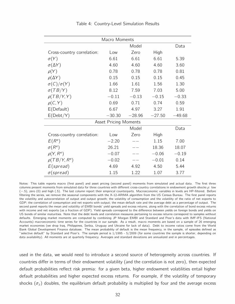
Table 4: Country-Level Simulation Results

Macro Moments

Model Data

Cross-country correlation: Low Zero High

σ(Y ) 6.61 6.61 6.61 5.39

σ(∆Y ) 4.60 4.60 4.60 3.60

ρ(Y ) 0.78 0.78 0.78 0.81

ρ(∆Y ) 0.15 0.15 0.15 0.45

σ(C)/σ(Y ) 1.66 1.61 1.56 1.30

σ(TB/Y ) 8.12 7.59 7.03 5.00

ρ(TB/Y, Y ) −0.11 −0.13 −0.15 −0.33

ρ(C, Y ) 0.69 0.71 0.74 0.59

E(Default) 6.67 4.97 3.27 1.91

E(Debt/Y) −30.30 −28.96 −27.50 −49.68

Asset Pricing Moments

Model Data

Cross-country correlation: Low Zero High

E(Re) −2.20 −− 1.15 7.00

σ(Re) 26.21 −− 18.36 18.07

ρ(Y,Re) −0.07 −− −0.06 −0.19

ρ(TB/Y,Re) −0.02 −− −0.01 0.14

E(spread) 4.69 4.92 4.50 5.44

σ(spread) 1.15 1.22 1.07 3.77

Notes: This table reports macro (first panel) and asset pricing (second panel) moments from simulated and actual data. The first three

columns present moments from simulated data for three countries with different cross-country correlations in endowment growth shocks ρ: low

(−.5), zero (0) and high (.5). The last column report their empirical counterparts. Macroeconomic variables in levels are HP-filtered. Before

filtering the series, we remove the seasonal components with the X-12-ARIMA algorithm from the US Census Bureau. The first panel reports

the volatility and autocorrelation of output and output growth; the volatility of consumption and the volatility of the ratio of net exports to

GDP; the correlation of consumption and net exports with output; the mean default rate and the average debt as a percentage of output. The

second panel reports the mean and volatility of EMBI bonds’ yield spreads and excess returns, along with the correlation of bond excess returns

with income and net exports (as a fraction of GDP). Yield spreads correspond to the difference between yields on foreign bonds and yields on

US bonds of similar maturities. Note that the debt levels and correlation measures pertaining to excess returns correspond to samples without

defaults. Emerging market moments are computed by combining JP Morgan EMBI and Standard and Poor’s data with IMF-IFS (National

Accounts) macroeconomic time series for the countries in our sample. As a result, macro moments are based on a sample of 26 emerging

market economies (we drop Iraq, Philippines, Serbia, Uruguay and Ukraine for lack of data). Debt to income ratios come from the World

Bank Global Development Finance database. The mean probability of default is the mean frequency, in the sample, of episodes defined as

”selective default” by Standard and Poor’s. The sample period is 1/1995 - 5/2009 (for some countries the sample is shorter, depending on

data availability). All moments are at quarterly frequency. Averages and standard deviations are annualized and in percentages.

used in the data, we would need to introduce a second source of heterogeneity across countries. If

countries differ in terms of their endowment volatility (and the correlation is not zero), then expected

default probabilities reflect risk premia: for a given beta, higher endowment volatilities entail higher

default probabilities and higher expected excess returns. For example, if the volatility of temporary

shocks (σz) doubles, the equilibrium default probability is multiplied by four and the average excess

32

return more than doubles. As a result, introducing heterogeneity in endowment volatilities and sorting

countries on default probabilities would also produce a cross-section of excess returns, similar to the

one we obtain in the data by sorting on ratings. This additional cross-section would naturally be priced

by the same risk factor. As previously noted, we keep the model simple and only introduce one key

source of heterogeneity, the cross-country correlation of endowment shocks.

At the end of each period t, we thus sort all countries into 6 portfolios on the basis of market

betas (βMkt). The 6 portfolios are re-balanced at the end of every period. For each portfolio j , we

compute the excess returns r e,jt+1 by taking the average of the excess returns in the portfolio. Excess

returns correspond to the returns in emerging countries minus the risk-free rate in the large, developed

economy. Table 5 provides an overview of the 6 portfolios.

Table 5: Portfolios of Simulated Data

Portfolios 1 2 3 4 5 6

Stock market beta: βMkt (Pre-Formation)

Mean −0.25 −0.12 −0.05 0.00 0.05 0.13

Std 0.20 0.15 0.11 0.10 0.10 0.13

Default probability

Mean 5.85 5.41 4.89 4.50 4.17 3.84

Std 1.33 1.21 1.09 1.02 0.96 0.91

Excess return: r e

Mean −1.24 −0.66 −0.14 0.29 0.52 0.65

Std 21.06 19.73 18.64 17.88 17.28 16.68

Std* 1.02 1.01 1.01 1.02 1.03 1.04

Debt/Output

Mean 30.14 29.71 29.29 29.01 28.67 28.52

Std 7.09 6.92 6.78 6.73 6.73 6.67

Stock market beta: βMkt (Post-Formation)

Mean −0.14 −0.08 −0.04 0.00 0.03 0.05

Std 0.01 0.01 0.01 0.01 0.01 0.01

Notes: This table reports, for each portfolio j , the average slope coefficient βMkt (pre-formation) from a regression of one-quarter sovereign

bonds’ excess returns on the investors’ stock market excess returns (first panel), the average expected probability of default (second panel),

the average excess return (third panel), the debt to output ratio (fourth panel) and the post-formation betas (fifth panel). Post-formation

betas correspond to slope coefficients in regressions of quarterly portfolios’ excess returns on quarterly investor’s stock market excess returns.

Probabilities of default, excess returns and debt ratios are reported in percentage points. Excess returns and default probabilities are annualized.

For each variable, the table reports its mean and its standard deviation. For excess returns, the table also reports standard deviations (denoted

Std∗) in samples without defaults.

The first panel reports the average βjMkt for countries in portfolio j . Business cycles of countries

with low βMkt are negatively correlated with the investors’ consumption growth. These countries on

average default more frequently when investors’ consumption is high and above their habit levels. On

the contrary, countries with high βMkt default more frequently when investors’ consumption is low and

33

close to their habit levels.16 The second panel reports average expected default probabilities. Sorting

on βMkt implies a cross-section of average default probabilities, with a spread of 2 percent. Note that

high beta countries have lower default probabilities than low beta countries.

Let us turn now to average excess returns. The larger the market βjMkt , the higher the excess

returns. This is exactly what we expect. Higher beta countries are riskier because their bonds pay

badly in bad times for investors, and thus they should offer higher excess returns on average. The

model produces average excess returns that range from -1.2 percent to 0.7 percent per annum. In

the model, some countries are good hedges to US consumption growth risk, and thus the negative

average excess returns. We do not find so perfect hedges in the data. This discrepancy is due to our

distribution of correlation coefficients, which is for simplicity symmetric around 0. More importantly,

the difference in excess returns between low and high beta countries in the model is large and amounts

to 190 basis points annually. Those excess returns, however, are lower than in the data. They also

appear much more volatile than in the data. Again, this volatility reflects our assumption that recovery

rates are zero in case of defaults. In samples without defaults, standard deviations are much lower

and close to 1 percent.

Matching means and variances of sovereign bond excess returns would certainly necessitate to look

at longer maturities. To show that maturities matter, we report in Table 9 of Appendix A the mean

senior CDS rates at different horizons for countries in our sample. Our dataset comprises series for 1,

2, .. 10-year horizons over a short sample. We obtain the fitted CDS curves by spline interpolation of

existing CDS contracts. We impose the boundary condition that the CDS rates tend to 0 when the

horizon tends to 0 (i.e, there is no instantaneous risk of default). We compute fitted values only when

at least the 1-year, 5-year and 10-year CDS rates are available. We find that, on average, 10-year

rates are more than 5 times higher than 3-month rates. As a result, we do not attempt to match

EMBI returns with our one-period model.

The model produces reasonable levels of debt to GDP ratios of around 30 percent, but lower than

the average of 45 percent measured in our sample. The spread in returns due to market betas is

not due to higher levels of debt. It is actually the opposite: high beta countries tend to pay higher

interest rates even if they borrow less in equilibrium. These features echo the characteristics of our

EMBI bond portfolios and illustrate the role of risk premia.

Finally, we run on simulated data the same asset pricing experiment as on actual data. Using

the simulated US stock market return as a risk factor, we obtain a clear cross-section of portfolio

betas, as reported in the last panel of Table 5. Appendix C, and particularly Table 20 there, reports

additional asset pricing results. The cross-sectional R2 is equal to 95% and the market price of risk

is in line with the average US stock market return. Our model offers a natural interpretation of our

empirical facts.

16Figures 8 and 9 in Appendix C illustrate this point; they present average consumption paths in the borrowing and

lending countries around default episodes in the case of positively correlated business cycles.

34

4.5 Implications

We end this paper by succinctly presenting some additional implications of the model regarding the

interest rate elasticity of debt levels, the correlations between output and interest rates, and the large

increase in yields in the fall of 2008. More broadly, the model implies that monetary unions might lead

to higher borrowing costs for some members because of higher business cycles’ synchronizations. We

simply highlight here the connections to our findings, as potential avenues for future research. But

we do not claim to solve any of these puzzles and acknowledge that each of these topics connects to

a large literature and deserves further study.

Interest rate elasticity of debt The link between interest rates and debt levels seems obvious:

interest rates are expected to rise when debt levels increase, because default probabilities increase.

Yet, this link is empirically elusive. Edwards (1984) finds that the external debt to GDP ratio plays a

significant role in explaining country spreads. More recently, however, Uribe and Yue (2006) do not

find any significant role for debt to GDP ratios. We can offer an explanation that reconciles these

findings. Looking back at our portfolios, we see that an increase in debt to GDP ratios goes along

with a worsening of S&P ratings and an increase in spreads for either low or high beta bonds. But

across beta groups, there is no clear pattern. The highest spreads do not correspond to the highest

debt levels. In other words, for a given beta, there might be a link between interest rates and debt

levels but there is no unconditional relation between the two.

Output-interest rate correlations Interest rates in emerging markets are in general counter-cyclical

with respect to their own GDP. But there exist large variations in the correlation coefficients between

output and interest rates.17 Our model offers an interpretation of this heterogeneity.

Recall that interest rates reflect default probabilities and covariances. On the one hand, if the

borrowers’ output is positively correlated with the US output, then we should expect high interest

rates in bad times: both the risk neutral (default probability) and the risk premium (due to investors’

time varying risk aversion) should be high in bad times. This mechanism leads to a very negative

correlation between interest rates and output in the emerging country. On the other hand, if the

borrowers’ output is negatively correlated with the US output, then the risk premium should now be

lower, leading to a higher correlation between interest rates and output. It is, however, difficult to

test this prediction since emerging countries do not offer long and high frequency measures of GDP

growth rates.18

17Uribe and Yue (2006) for example estimate the following correlations between 1994 and 2001: −0.67 in Argentina,

−0.51 in Brazil, −0.80 in Ecuador, −0.58 in Mexico, −0.37 in Peru, −0.02 in the Philippines, and −0.07 in South Africa.

The first four are significantly different from zero; the others are not.18At least, our data do not seem to reject this reasoning. Looking at the correlation between the HP-filtered US and

foreign GDP series, we obtain a high and positive correlation for Argentina (0.51) and Mexico (0.52) and a somehow lower

but still positive correlation for Brazil (0.11) – see Table 10 in the separate appendix. These countries are characterized

by highly counter-cyclical interest rates. The Philippines, Peru and South Africa have both a-cyclical interest rates and

35

Fall 2008 Eichengreen and Mody (2000) attribute past variations in emerging market spreads to

investor sentiment. We offer a different perspective. We show in this paper that average returns on

EMBI bonds satisfy a no-arbitrage condition. Variations in spreads are thus at least partly rational,

and not only behavioral, responses to economic conditions. We apply this reasoning to the large

increase in sovereign bond spreads in the fall of 2008.

Our conditional asset pricing results show that the market price of risk increases in bad times, e.g

when the option-implied VIX index is high. The fall of 2008 indeed corresponds to a five-standard

deviation shock to this index. A higher market price of risk implies higher expected excess returns in

the future and thus lower prices now. During this period, we also observe an increase in the quantity

of risk. This increase in betas also implies higher expected returns and lower prices, but the model

does not capture this second effect, as the quantity of risk is fixed. The model, however, implies

large variations in the market price of risk. Feeding the model with the actual US consumption

growth series, we obtain a doubling of the market price of risk during the mortgage crisis.19 This

time-variation in risk-aversion implied by the model accounts for large changes in bond prices, but it

is not enough to replicate the sudden drop and rapid rebound experienced on emerging bond markets.

Additional factors, either behavioral or due to additional sources of risk, are needed to fully account

for this episode.

Monetary unions Finally, we note that our results offer a new perspective on monetary unions. At

the time of this writing, several European countries face high borrowing costs compared to Germany

for example. Our paper focuses on US investors buying emerging market debt issued in US dollars.

A similar reasoning, however, applies to German investors buying the debt of other members of the

euro area. Insofar as monetary unions entail convergence across business cycles (and thus higher

correlations and betas), they may imply higher borrowing difficulties, particularly acute in bad times,

because of sovereign risk premia. By removing currency risk premia, however, currency unions also

affect interest rates. We leave the study of the interaction between sovereign and currency risk premia

out for future research.

5 Conclusion

In this paper, we show that emerging market betas impact sovereign bond prices and that risk matters

on these markets. In the data, countries with higher bond betas pay higher borrowing rates. The

difference in spreads between countries with high and low betas is large, as large actually as the

difference between low and high default probabilities. The leading structural models of sovereign debt

assume that investors are risk-neutral and thus cannot account for our empirical findings.

low correlation with the US (-0.12, -0.21 and 0.02).19Figure 10 in the appendix reports the time-series of the maximal Sharpe ratio in the model during the period from

1995:I to 2009:II.

36

We propose one example of a general equilibrium model of sovereign borrowing and default with

risk-averse investors. In the model, borrowing countries only differ along one dimension: their endow-

ments are more or less correlated to the lenders’ consumption. Lenders’ habit preferences lead to

spreads in returns between low and high default probability countries and between high and low beta

countries, albeit smaller than in the data. The model illustrates the impact of lenders’ time-varying

risk aversion on borrowers’ default decisions.

Our empirical methodology and our general equilibrium model are relevant to address default risk

premia in other contexts. The literature on consumer bankruptcy faces endogenous decisions to

default that are similar to the ones described in this paper. Notable examples include Chatterjee,

Corbae, Nakajima and Rios-Rull (2007) and Livshits, MacGee and Tertilt (2007). Likewise, firm

dynamics depend on financial market features and endogenous defaults, as shown in Cooley and

Quadrini (2001). These papers, however, consider only risk-neutral financial intermediaries. Our work

shows that lenders’ risk aversion affect both debt quantities and prices.

References

Adler, Michael and Rong Qi, “Long-Duration Bonds and Sovereign Defaults,” Emerging MarketsReview, 2003, 4, 91–120.

Aguiar, Mark and Gita Gopinath, “Defaultable debt, interest rates and the current account,” Journalof International Economics, 2006, 69, 64–83.

and , “Emerging Market Business Cycles: The Cycle is the Trend,” Journal of PoliticalEconomy, 2007, 115 (1), 69–101.

Almeida, Heitor and Thomas Philippon, “The Risk-Adjusted Costs of Financial Distress,” Journalof Finance, 2007, 62 (6), 2557 – 2586.

Alvarez, Fernando E. and Urban J. Jermann, “Efficiency, Equilibrium, and Asset Pricing with Riskof Default,” Econometrica, 2000, 68 (4), 775–798.

Amador, Manuel, “Sovereign Debt and the Tragedy of the Commons,” 2008. Working Paper,Stanford University.

Andrade, Sandro C., “A Model of Asset Pricing under Country Risk,” Journal of International Moneyand Finance, 2009, 28 (4), 671–695.

Andrews, Donald W.K., “Heteroskedasticity and Autocorrelation Consistent Covariance Matrix Es-timation,” Econometrica, 1991, 59 (1), 817–858.

Arellano, Cristina, “Default Risk and Income Fluctuations in Emerging Economies,” American Eco-nomic Review, 2008, 98 (3), 690–712.

and Ananth Ramanarayanan, “Default and the Term Structure in Sovereign Bonds,” 2009.Working Paper.

Atkeson, Andrew, “International Lending with Moral Hazard and Risk of Repudiation,” Economet-rica, July 1991, 59 (4), 1069–1089.

Bansal, Ravi and Amir Yaron, “Risks for the Long Run: A Potential Resolution of Asset PricingPuzzles,” Journal of Finance, August 2004, 59, 1481–1509.

Barro, Robert, “Rare Disasters and Asset Markets in the Twentieth Century,” Quarterly Journal ofEconomics, 2006, 121, 823.

37

Bekaert, Geert and Campbell R. Harvey, “Time-Varying World Market Integration,” Journal ofFinance, 1995, 50 (2), 403–444.

and , “Foreign Speculators and Emerging Equity Markets,” Journal of Finance, 2000, 55(2), 565 – 613.

, , and Christian Lundblad, “Liquidity and Expected Returns: Lessons from EmergingMarkets,” Review of Financial Studies, 2007, 20 (6), 1783–1832.

Benjamin, David and Mark L. J. Wright, “Recovery Before Redemption: A Theory of Delays inSovereign Debt Renegotiations,” 2009. Working paper UCLA.

Bhamra, Harjoat S., Lars-Alexander Kuehn, and Ilya A. Strebulaev, “The Levered Equity RiskPremium and Credit Spreads: A Unified Framework,” Review of Financial Studies, 2010, 23,546–703.

Boehmer, Ekkehart and William L. Megginson, “Determinants of Secondary Market Prices forDeveloping Country Syndicated Loans,” Journal of Finance, 1990, 45 (5), 1517–1540.

Bolton, Patrick and Olivier Jeanne, “Structuring and Restructuring Sovereign Debt: The Role ofa Bankruptcy Regime,” Journal of Political Economy, 2007, (115 (6)), 901–924.

Broner, Fernando A., Guido Lorenzoni, and Sergio L. Schmukler, “Why Do Emerging EconomiesBorrow Short Term,” 2008. Working Paper MIT.

Broner, Fernando, Alberto Martin, and Jaume Ventura, “Sovereign Risk and Secondary Markets,”American Economic Review, 2010, 100, 1523–1555.

Bulow, Jeremy and Kenneth Rogoff, “Sovereign Debt: Is to Forgive to Forget?,” American Eco-nomic Review, 1989, 79 (1), 43–50.

Campbell, John Y. and John H. Cochrane, “By Force of Habit: A Consumption-Based Explanationof Aggregate Stock Market Behavior,” Journal of Political Economy, April 1999, 107 (2), 205–251.

Cavanagh, John and Richard Long, “Methodology Brief: Introducing the J.P. Morgan EmergingMarkets Bond Index Global,” 1999. J.P. Morgan Emerging Market Research.

Chatterjee, S., D. Corbae, M. Nakajima, and J. Rios-Rull, “A Quantitative Theory of UnsecuredConsumer Credit with Risk of Default,” Econometrica, 2007, 75 (6), 1525 – 1589.

Chatterjee, Satyajit and Burcu Eyigungor, “Maturity, Indebtedness, and Default Risk,” April 2010.Federal Reserve Bank of Philadelphia Working Paper.

Chen, Long, Pierre Colin-Dufresne, and Robert S. Goldstein, “On the Relation Between CreditSpread Puzzles and the Equity Premium Puzzle,” Review of Financial Studies, 2008, 22 (9),3367–3409.

Chien, YiLi and Hanno Lustig, “The Market Price of Aggregate Risk and the Wealth Distribution,”Review of Financial Studies, 2010, 23, 1596–1650.

Cochrane, John H., Asset Pricing, Princeton, NJ: Princeton University Press, 2001.

Cole, Harold L. and Timothy J. Kehoe, “Self-Fulfilling Debt Crises,” Review of Economic Studies,2000, 67, 91–216.

Cooley, Thomas F. and Vincenzo Quadrini, “Financial Markets and Firm Dynamics,” AmericanEconomic Review, 2001, 91 (5), 1286–1310.

Duffie, Darrell, Lasse H. Pedersen, and Kenneth J. Singleton, “Modeling Sovereign Yield Spreads:A Case Study of Russian Debt,” Journal of Finance, 2003, 83 (1).

Eaton, Jonathan and Mark Gersovitz, “Debt with Potential Repudiation: Theoretical and EmpiricalAnalys,” Review of Economic Studies, April 1981, 48 (2), 289–309.

38

Edwards, Sebastian, “LDC Foreign Borrowing and Default Risk: An Empirical Investigation, 1976-80,” American Economic Review, 1984, 74 (4), 726–734.

Eichengreen, Barry and A Mody, “What explains changing spreads on emerging-market debt: fun-damentals or market sentiment?,” in Sebastian Edwards, ed., Capital flows and the emergingeconomies : theory, evidence, and controversies, Chicago University Press, 2000.

Fama, Eugene and James MacBeth, “Risk, Return, and Equilibrium: Empirical Tests,” Journal ofPolitical Economy, 1973, 81, 3–56.

Favero, Carlo, Marco Pagano, and Ernst-Ludwig von Thadden, “How Does Liquidity Affect BondYields?,” Journal of Financial and Quantitative Analysis, 2010, 45 (1), 107–134.

Fostel, Ana and John Geanakoplos, “Leverage Cycles and the Anxious Economy,” American Eco-nomic Review, 2008, 98 (4), 1211–1244.

Gabaix, Xavier, “Variable Rare Disasters: An Exactly Solved Framework for Ten Puzzles in MacroFinance,” November 2008. Working Paper NYU Stern.

Garleanu, Nicolae and Stavros Panageas, “Young, Old, Conservative, and Bold: The Implicationsof Heterogeneity and Finite Lives for Asset Pricing,” April 2008. Working paper UC Berkeley.

Gelos, Gaston R., Ratna Sahay, and Guido Sandleris, “Sovereign Borrowing by Developing Coun-tries: What Determines Market Access?,” 2004. IMF Working Paper 221.

Giesecke, Kay, Francis A. Longstaff, Stephen Schaefer, and Ilya Strebulaev, “Corporate BondDefault Risk: A 150-Year Perspective,” 2010. Working Paper UCLA.

Gilchrist, Simon, Vladimir Yankov, and Egon Zakrajsek, “Credit Supply Shocks: Evidence fromCorporate Bond and Stock Markets,” Journal of Monetary Economics, 2009, 56 (4), 471–493.

Hansen, Lars Peter, “Large Sample Properties of Generalized Method of Moments Estimators,”Econometrica, 1982, 50, 1029–54.

and Scott F. Richard, “The Role of Conditioning Information in Deducing Testable RestrictionsImplied by Dynamic Asset Pricing Models,” Econometrica, 1987, 55 (3), 587–613.

Hatchondo, Juan Carlos and Leonardo Martinez, “Long-Duration Bonds and Sovereign Defaults,”Journal of International Economics, 2009, 79, 117–125.

, , and Horacio Sapriza, “Quantitative Models of Sovereign Defaults and the Threat ofFinancial Exclusion,” Economic Quarterly, 2007, 93 (3), 251–286.

Hilscher, Jens and Yves Nosbusch, “Determinants of Sovereign Risk: Macroeconomic Fundamen-tals and the Pricing of Sovereign Debt,” Review of Finance, 2010, 14, 235 – 262.

Kehoe, Timothy J. and David K. Levine, “Debt-Constrained Asset Markets,” Review of EconomicStudies, 1993, 60, 868–888.

Kovrijnykh, Natalia and Balazs Szentes, “Equilibrium Default Cycles,” Journal of Political Econ-omy, June 2007, 115 (3), 403–446.

Lettau, Martin and Sydney Ludvigson, “Measuring and Modeling Variation in the Risk-ReturnTradeoff,” in Yacine Ait-Sahalia and Lars Peter Hansen, eds., Handbook of Financial Economet-rics, Elsevier, 2009.

Livshits, Igor, James MacGee, and Michele Tertilt, “Consumer Bankruptcy: A Fresh Start,”American Economic Review, 2007, 97 (1), 402 – 418.

Lizarazo, Sandra Valentina, “Default Risk and Risk Averse International Investors,” 2010. Workingpaper ITAM.

Longstaff, Francis A., Jun Pan, Lasse H. Pedersen, and Kenneth J. Singleton, “How Sovereignis Sovereign Credit Risk?,” American Economic Journal: Macroeconomics, 2011, forthcoming.

39

Lustig, Hanno and Adrien Verdelhan, “Business Cycle Variation in the Risk-Return Tradeoff,” 2010.Working Paper.

Martin, Ian, “Consumption-Based Asset Pricing with Higher Cumulants,” 2008. Working PaperStanford University.

Mehra, R. and E. Prescott, “The Equity Premium: A Puzzle,” Journal of Monetary Economics,1985, 15, 145–161.

Mendoza, Enrique G. and Vivian Z. Yue, “A Solution to the Default Risk Business Cycle Discon-nect,” June 2008. NBER Working Paper 13861.

Neumeyer, Pablo and Fabrizio Perri, “Business Cycles in Emerging Economies: The Role of InterestRates,” Journal of Monetary Economics, 2005, 52 (2), 345–380.

Newey, Whitney K. and Kenneth D. West, “A Simple, Positive Semi-Definite, Heteroskedasticityand Autocorrelation Consistent Covariance Matrix,” Econometrica, 1987, 55 (3), 703–708.

Pan, Jun and Kenneth J. Singleton, “Default and Recovery Implicit in the Term Structure ofSovereign CDS Spreads,” Journal of Finance, October 2008, 5, 2345–2384.

Patton, Andrew J. and Allan Timmermann, “Monotonicity in Asset Returns: New Tests with Appli-cations to the Term Structure, the CAPM and Portfolio Sorts,” Journal of Financial Economics,forthcoming, 2010.

Pouzo, Demian, “Optimal Taxation with Endogenous Default Under Incomplete Markets,” 2009.Working Paper, Berkeley University.

Rietz, Thomas A., “The Equity Risk Premium: A Solution?,” Journal of Monetary Economics, 1988,22 (1), 117–131.

Rose, Andrew, “One Reason Countries Pay their Debts: Renegotiation and International Trade,”Journal of Development Economics, 2005, 77 (1), 189–206.

Ross, Stephen A., “The Arbitrage Theory of Capital Asset Pricing,” Journal of Economic Theory,1976, 13, 341–360.

Shanken, Jay, “On the Estimation of Beta-Pricing Models,” The Review of Financial Studies, 1992,5 (2), 1–33.

Tomz, Micheal, Reputation and International Cooperation, Sovereign Debt across Three Centuries,Princeton, NJ: Princeton University Press, 2007.

Uribe, Martin and Vivian Yue, “Country Spreads and Emerging Markets: Who Drives Whom?,”Journal of International Economics, June 2006, 69, 6–36.

Verdelhan, Adrien, “A Habit-Based Explanation of the Exchange Rate Risk Premium,” Journal ofFinance, 2010, 65 (1), 123–145.

Wachter, Jessica, “A Consumption-Based Model of the Term Structure of Interest Rates,” Journalof Financial Economics, 2006, 79, 365–399.

Weil, Philippe, “The Equity Premium Puzzle and the Risk-Free Rate Puzzle,” Journal of MonetaryEconomics, 1989, 24, 401–424.

Yue, Vivian Z., “Sovereign Default and Debt Renegotiation,” Journal of International Economics,2010, 80 (2), 176–187.

Zame, William R., “Efficiency and the Role of Default when Security Markets are Incomplete,”American Economic Review, 1993, 83 (5), 1142–1164.

40

Sovereign Risk Premia

- Supplementary Online Appendix -

NOT FOR PUBLICATION

This separate Appendix contains three sections. Appendix A reports additional statistics on our data set.

Appendix B describes our asset pricing methodology and reports additional asset pricing results. Appendix C

details our computational algorithm and reports additional simulation results.

Appendix A Data

Cavanagh and Long (1999) offer a detailed description of the construction of EMBI indices. As a snapshot of

our data set, Figure 4 reports, for each country in the JP Morgan’s EMBI Global Index, the annual stripped

spread plotted against the Standard and Poor’s credit rating at the end of May 2009. The stripped spread is

equal to the difference between the average yield to maturity in the emerging country and the corresponding

yield to maturity on the US Treasury spot curve, after ‘stripping’ out the value of any collateralized cash flows.

These spreads increase on average when credit ratings worsen. But, for any given rating, there exists a lot of

heterogeneity in spreads. These two characteristics of sovereign spreads motivate our study.

We report below additional descriptive statistics on our data.

• Table 6 reports summary statistics on the EMBI stripped spreads for our sample. All spreads are annual.

• Table 7 presents the market value of US holdings of long term foreign government debt.

• Table 8 reports the ratio of debt to GDP for the countries in our sample, using data from the Global

Development Finance dataset of the World Bank.

• Table 9 reports mean senior CDS rates at different horizons for countries in our sample.

• Table 10 reports the cross-country correlation coefficients between each EMBI country’s real GDP and

the US real GDP. We consider either annual or quarterly data. We extract their cyclical components using

a HP filter (with the appropriate bandwidth parameter: 100 on annual and 1600 on quarterly data). At

annual frequency, we use all available data and thus start at different dates for each country. At quarterly

frequency, we consider one common sample (1994 - 2008) and ignore countries with incomplete series

over that sample. We obtain correlation coefficients ranging from -0.3 to 0.6 on annual data and from

-0.3 to 0.5 on quarterly data. These estimates are inherently imprecise: they rely on less than 60

observations.

Appendix B Asset Pricing Tests

We briefly describe here the asset pricing tests used in the text. See Cochrane (2001) for a comprehensive

presentation and discussion. We then report additional asset pricing results.

41

GMM The moment conditions are the sample analog of the populations pricing errors:

gT (b) = ET (mt r̃et ) = ET (r̃ et )− ET (r̃ et f

′t )b,

where r̃ et = [r̃ e,1t , r̃ e,2t , ..., r̃ e,Nt ]′ groups all the N EMBI portfolios. In the first stage of the GMM estimation,

we use the identity matrix as the weighting matrix, while in the second stage we use the inverse of the spectral

density S matrix of the pricing errors in the first stage: S =∑E[(mt r̃

et )(mt−j r̃

et−j)

′].20 We use demeaned

factors in both stages. Since we focus on linear factors models, the first stage is equivalent to an OLS cross-

sectional regression of average returns on the second moment of returns and factors. The second stage is a

GLS cross-sectional regression of average excess returns on the second moment of returns and factors.

FMB In the first stage of the FMB procedure, for each portfolio j , we run a time-series regression of the

EMBI excess returns r̃ et on a constant and the factors ft , in order to estimate βj . The only difference with the

first stage of the GMM procedure stems from the presence of a constant in the regressions. In the second stage,

we run a cross-sectional regression of the average excess returns ET (mt r̃et ) on the betas that were estimated in

the first stage, to estimate the factor prices λ. The first stage GMM estimates and the FMB point estimates

are identical, because we do not include a constant in the second step of the FMB procedure. Finally, we can

back out the factor loadings b from the factor prices and covariance matrix of the factors.

Robustness Checks This section reports robustness checks: additional statistics, different sorts, different

risk factors and conditional asset pricing results.

• Table 11 reports how frequently countries change portfolios.

• Figure 5 plots for Argentina and Mexico – as an example – the monthly S&P credit rating, the bond

market beta βEMBI and the portfolio allocation.

• Table 12 reports additional statistics for our benchmark portfolios of countries sorted on credit ratings

and bond market betas.

• Figure 6 plots average rolling betas for each benchmark portfolio along with NBER recessions and financial

crisis dates. Theses dates are from Kho, Bong-Chan, Dong Lee and Rene M. Stulz, (2000), American

Economic Review, 90 (2), p28-31.

• Table 13 reports summary statistics for portfolios of countries sorted on credit ratings and bond market

betas. Statistics are value-weighted.

• Table 14 reports similar information for portfolios of countries sorted on credit ratings and stock market

betas. Statistics are equally-weighted.

• Table 15 reports asset pricing results obtained with the equally-weighted portfolios presented in Table

14. The sole risk factor is the return on a US BBB bond index.

20We use a Newey and West (1987) approximation of the spectral density matrix The optimal number of lags is

determined using Andrews (1991)’s criterion with a maximum of 6 lags.

42

• Figure 7 compares expected and realized average excess returns obtained with the equally-weighted

portfolios presented in Table 14.

• Table 16 reports the results of our conditional asset pricing tests using VIX as the conditioning variable.

• Table 17 reports asset pricing results obtained with the log change in the VIX index as risk factor.

• Table 18 reports asset pricing results obtained with the log change in the VIX index and the return on a

US BBB bond index as risk factors.

• Table 19 reports asset pricing results obtained with the TED spread as risk factor.

Appendix C Simulations

Computational Algorithm To solve the model numerically we de-trend all the Bellman equations. To do

so, we normalize all variables by µgΓt−1.

Hatchondo, Martinez, and Sapriza (2010) show that evenly spaced and coarse grids imply biases in the mean

debt levels and volatility of spreads. To alleviate the biases, we discretize the borrower’s endowment process

using non evenly spaced grid points that span -5 to +5 standard deviations around the mean of each process.

Most of the grid points are between one and three standard deviations around the means. We discretize the

investors’ surplus consumption ratio in 6 grid points equally spaced between .0072 and Smax . We build the

transition matrix as described in Tauchen and Hussey (1991). The quantity of debt is discretized between 0

(no debt) and -0.95 and we check in our simulations that this constraint never binds. Most grid points are

between -20% and +20% around the mean debt level. The exact definition of our grids and our programs are

available on our websites.

We start with a guess for the bond price function Q0(B′, x) = Qr f for each B′ and x , where Qr f is the

price of the risk free bond available to investors and is equal to Qr f = E[M ′] and x = [y , s]′ is a vector

containing the exogenous state variables. Given the bond price function, we use value function iteration to

obtain the optimal consumption, asset holdings and default policy functions. Given the optimal default policy

function found in the previous step, we update the bond price function Q1(B′, x) according to equation 3.3. If

a convergence criterion is satisfied, we stop. If not, we use the updated price function to compute new values

for the optimal consumption, asset holdings and default policy functions and repeat this routine up to the point

that max{Qi(B′, x)−Qi+1(B′x)} < 10−6.

We also compute the price of a claim on total consumption and its return. To obtain the equilibrium price-

dividend ratio in the Campbell and Cochrane (2009) model, we follow Wachter (2005). In our simulation, the

price-dividend ratio has a mean of 17.85 and a standard deviation of 13.13 (both annualized), and a quarterly

autocorrelation of 0.97.

Due to the large number of state variables and the large number of countries, we run our code in parallel

mode on 32 processors. We start with small grids and interpolate the obtained value functions to use them

as initial guesses for larger grids. We have a total of 36 simulated countries, for 90,000 quarters; we use the

second half of the sample for our analysis.

We reproduce on simulated data the same experiment that we run on actual data. Table 20 reports asset

pricing results on portfolios of simulated data. We use the US stock market return as our risk factor. We obtain

43

a positive and significant market price of risk that is in line with the mean of the risk factor. This unique risk

factor explains 95% of the cross-section of average sovereign bond excess returns. The alphas are overall small

and not statistically significant at the 1% level. For the high beta portfolios, however, the alphas are individually

significant. This result is in line with the model: the investors’ preferences imply that the market price of risk is

time-varying and cannot be perfectly summarized by a unique risk factor. We also obtain a clear cross-section

of betas. High beta countries offer high sovereign risk premia. This is in line with the data: as shown in the

last panel of Tables 12, 13, and 14, high (pre-formation) beta portfolios exhibit high (post-formation) stock

market betas. Note that the time-series R2 are small because of missing risk factors (higher order terms in the

log linearization of the stochastic discount factor), idiosyncratic variations and our assumption of zero recovery

rates in case of defaults.

Time Series Figures 8 and 9 present the average consumption growth of lenders and borrowers before and

after defaults.

Figure 10 reports the time-series of the Sharpe ratio in the model, using actual consumption growth shocks

in the US.

44

A− BBB− BB− B− CCC− CC−0

500

1000

1500

2000

2500

3000

3500EMBI G and S&P Ratings as of May 2009

S&P Ratings

EM

BI G

Spr

ead

(bas

is p

oint

s)

ARG

BEL

BRA

BUL

CHILCHI

COL

DOM

ECU

EGY

EL

HUN

IND

KAZ

LEB

MALMEX

PAK

PANPER PHI

POL

RUS

SER

SOU TUN

UKR

URU

VEN

VIE

Figure 4: EMBI Global Annual Spreads and Standard and Poor’s Ratings

The figure plots, for each country in the EMBI Global Index, the annual stripped spread against the Standard and Poor’s credit rating at the

end of May 2009. Spreads are in basis points. Standard and Poor’s credit ratings are indexed from 1 (AAA) to 23 (SD). A higher number

implies a lower credit worthiness. Data are from Datastream.

45

Table 6: EMBI Global Annual Spreads

The table presents summary statistics on J.P. Morgan EMBI Global stripped spreads. All spreads are annual. We report the mean, standard

deviation, min, max, median, skewness, kurtosis and autocorrelation (AC) . The last column reports the total number N of observations for

each country in the sample. The stripped spread differs from the more standard ’blended’ spread because the values of any collateralized flows

are stripped from the bond, when computing the difference between the bond yield to maturity and the yield of a corresponding U.S. Treasury

bond. The standard deviation is computed using the monthly series of annual spread. Data are monthly, December 1993 - May 2009 and

available on Datastream.

EMBI Global Spread % Mean Std Min Max Median Skewness Kurtosis AC N

Argentina 18.00 20.38 1.93 70.78 7.42 1.29 2.96 0.97 186

Belize 8.60 4.95 3.67 17.90 6.51 0.98 2.35 1.00 27

Brazil 6.91 4.02 1.42 24.12 6.65 1.16 5.26 0.92 182

Bulgaria 6.16 5.19 0.56 21.54 5.30 0.89 2.88 0.95 179

Chile 1.48 0.71 0.55 3.92 1.46 1.01 4.11 0.94 121

China 1.08 0.51 0.44 3.57 1.05 1.47 6.83 0.86 183

Colombia 4.30 2.09 1.17 10.66 4.25 0.42 2.45 0.93 148

Cote D’Ivoire 23.37 7.54 5.86 34.76 24.83 −0.63 2.40 0.92 121

Dominican Republic 6.06 4.08 1.35 17.30 4.74 1.19 3.47 0.93 91

Ecuador 13.53 9.42 4.61 47.64 11.08 1.73 5.46 0.93 172

Egypt 1.91 1.32 0.25 5.43 1.36 0.86 2.59 0.94 95

El Salvador 2.99 1.49 1.20 8.61 2.67 2.13 7.76 0.93 86

Hungary 1.00 1.01 0.07 5.40 0.71 2.84 11.13 0.95 125

Indonesia 3.24 1.77 1.44 9.30 2.75 1.91 5.92 0.93 61

Iraq 6.41 2.29 4.23 12.82 5.46 1.54 4.13 0.91 38

Kazakhstan 6.41 3.80 1.84 13.71 4.70 0.67 1.96 0.89 24

Lebanon 4.29 2.14 1.29 10.52 3.78 1.18 4.06 0.96 134

Malaysia 1.91 1.49 0.40 10.55 1.56 2.81 13.98 0.93 152

Mexico 4.00 2.71 0.93 15.89 3.52 1.64 5.90 0.95 186

Morocco 3.83 2.43 0.54 16.06 3.92 1.36 7.40 0.84 107

Pakistan 6.16 5.65 1.42 21.32 3.36 1.38 3.66 0.96 82

Panama 3.47 1.18 1.17 6.79 3.56 −0.00 2.21 0.90 155

Peru 4.22 2.01 1.00 9.41 4.18 0.33 2.32 0.93 147

Philippine 4.11 1.45 1.38 9.37 4.23 0.51 4.13 0.90 138

Poland 2.04 1.57 0.35 8.71 1.83 1.75 6.64 0.95 176

Russia 9.22 12.83 0.90 57.83 4.15 2.21 6.96 0.96 138

Serbia 3.60 2.62 1.52 12.24 2.45 1.82 5.18 0.94 47

South Africa 2.35 1.37 0.67 6.55 2.18 1.11 4.04 0.95 174

Thailand 1.58 1.27 0.41 9.51 1.30 3.02 16.57 0.80 106

Trinidad and Tobago 3.07 2.41 0.00 9.55 2.68 1.11 3.57 0.64 25

Tunisia 1.73 1.10 0.49 5.35 1.42 1.33 4.05 0.95 85

Turkey 4.63 2.41 1.39 10.73 3.95 0.73 2.52 0.93 156

Ukraine 7.37 7.48 1.34 34.91 3.50 1.47 4.27 0.94 109

Uruguay 5.10 3.37 1.41 16.43 3.76 1.52 4.82 0.93 97

Venezuela 8.88 5.01 1.67 25.26 8.37 0.70 2.82 0.92 186

Vietnam 2.80 2.06 0.95 8.80 1.82 1.48 4.14 0.91 43

All 5.44 3.70 1.38 17.03 4.35 1.30 5.03 0.92 118

46

Table 7: US Holdings of Foreign Long Term Government Debt

The table presents the market value of US holdings of long term foreign government debt. Data are available in different pdf documents at

http : //www.treas.gov/tic/f pis.shtml#usclaims. The information comes from the surveys of Foreign Portfolio Holdings of US Securities.

We report here all the available years. For 2008, the table also reports the market value US holdings of long term foreign government debt

issued in US dollars (in the last column). Amounts in millions of US dollars.

Countries 1997 2001 2003 2004 2005 2006 2007 2008 2008 (USD)

Argentina 14112 1339 1341 1923 4058 7281 6079 2579 1794

Belize 0 0 32 14 9 25 27 49 49

Brazil 8189 8768 15234 16611 17822 14820 12580 15671 7476

Bulgaria 1041 1663 1437 1167 350 184 169 86 83

Chile 202 248 1891 1821 1501 1103 827 576 576

China 1534 171 579 481 406 464 332 363 361

Colombia 1337 2071 2903 3338 3464 4724 5059 4585 2340

Cote D’Ivoire 26 43 38 83 75 92 153 60 30

Dominican Republic 25 113 496 428 622 513 562 303 303

Ecuador 1366 672 853 1023 900 506 663 343 343

Egypt 0 248 48 46 981 1134 1632 1461 1258

El Salvador 1 15 506 626 791 897 788 474 474

Hungary 1152 267 564 575 491 422 1370 1009 87

Indonesia 259 61 362 594 1440 2107 2876 3725 2083

Iraq −− −− −− −− −− −− −− −− −−

Kazakhstan 63 110 5 11 9 11 0 0 0

Lebanon 438 31 97 155 285 265 272 179 179

Malaysia 161 557 1185 1394 1618 1650 2981 2604 390

Mexico 10916 11355 17947 18791 16751 12465 11949 10294 6946

Morocco 163 177 80 136 114 28 46 21 16

Pakistan 219 78 48 20 15 187 313 20 176

Panama 1848 1723 2808 2839 2898 2348 2211 1626 1626

Peru 673 1071 2878 3196 3688 2695 2926 270 1607

Philippines 1217 1646 2452 2638 3180 3541 3404 2166 2100

Poland 2448 1725 1536 2466 2750 4377 4737 2827 460

Russia 1843 5025 7466 9739 9215 7360 5729 4124 4124

Serbia 1 1 0 0 101 93 59 96 96

South Africa 1982 797 2451 2759 2260 2691 2998 1899 917

Thailand 801 212 341 503 644 757 65 397 0

Trinidad and Tobago 143 254 569 437 462 329 405 297 297

Tunisia 27 155 405 245 384 340 265 389 244

Turkey 640 1003 1813 2269 2898 3934 5107 3961 2216

Ukraine 2 189 585 1413 1079 1130 1337 748 559

Uruguay 301 512 520 717 925 1659 1711 1202 898

Venezuela 3758 2325 4101 5084 4556 4421 3946 2868 2693

Vietnam 24 20 81 113 306 231 233 192 192

All 56912 44645 73652 83655 87048 84784 83180 69118 42993

47

Table 8: External Debt EMBI Global countries

The table presents summary statistics on the ratio between total external debt to gross national product (GNP) for the sample of J.P. Morgan

EMBI Global countries. We report the mean, standard deviation, min, max, median. Data is from the World Bank Global Development Finance

(GDF) database for the period 1993-2007. All moments are computed using monthly series obtained by linear interpolation of the original GDF

annual series. No data is available for Hungary, Iraq, Trinidad and Tobago on the GDF database.

External Debt Mean Std Min Median Max

Argentina 0.66 0.35 0.28 0.51 1.53

Belize 0.75 0.26 0.35 0.79 1.18

Brazil 0.31 0.09 0.19 0.30 0.47

Bulgaria 0.84 0.17 0.58 0.86 1.14

Chile 0.46 0.09 0.32 0.43 0.64

China 0.14 0.02 0.12 0.14 0.19

Colombia 0.33 0.05 0.22 0.33 0.42

Cote D’Ivoire −− −− −− −− −−

Dominican Republic 0.34 0.07 0.25 0.30 0.53

Ecuador 0.70 0.17 0.41 0.70 1.05

Egypt 0.39 0.11 0.23 0.36 0.66

El Salvador 0.38 0.11 0.26 0.35 0.56

Hungary −− −− −− −− −−

Indonesia 0.74 0.30 0.34 0.63 1.68

Iraq −− −− −− −− −−

Kazakhstan 0.54 0.32 0.08 0.71 1.04

Lebanon 0.64 0.33 0.18 0.58 1.07

Malaysia 0.46 0.07 0.29 0.45 0.62

Mexico 0.32 0.11 0.17 0.27 0.60

Morocco 0.53 0.19 0.27 0.57 0.86

Pakistan 0.44 0.08 0.28 0.46 0.54

Panama 0.70 0.09 0.54 0.69 0.96

Peru 0.51 0.09 0.33 0.53 0.70

Philippine 0.64 0.10 0.42 0.64 0.78

Poland 0.38 0.06 0.27 0.38 0.53

Russia 0.43 0.18 0.26 0.34 0.93

Serbia 0.79 0.21 0.54 0.69 1.28

South Africa 0.17 0.03 0.13 0.18 0.23

Thailand 0.54 0.20 0.27 0.54 0.97

Trinidad and Tobago −− −− −− −− −−

Tunisia 0.65 0.06 0.57 0.64 0.77

Turkey 0.41 0.08 0.28 0.39 0.59

Ukraine 0.36 0.14 0.06 0.42 0.55

Uruguay 0.57 0.30 0.29 0.40 1.20

Venezuela 0.42 0.11 0.19 0.42 0.67

Vietnam 0.73 0.43 0.35 0.42 1.88

All 0.51 0.16 0.29 0.48 0.84

48

Table 9: CDS Curves for EMBI Global countries

The table presents mean senior CDS rates (in basis points) for the sample of J.P. Morgan EMBI Global countries at different horizons. The

last column reports the ratio of the 10-year (observed) to the 3-month (fitted) CDS rates. Our dataset comprises series for 1, 2, .. 10-year

horizons. We obtain the fitted CDS curves by spline interpolation of the rates from existing CDS contracts. We impose the boundary condition

that the CDS rates tend to 0 when the horizon tends to 0. We compute fitted values only when at least the 1-year, 5-year and 10-year CDS

rates are available. We do not have data for Belize, Cote d’Ivoire, Dominican Republic, Trinidad and Tobago and Uruguay. The sample period

is 1/2003-5/2009, but most series start later than January 2003.

3-month 1-year 5-year 10-year Slope 10-yr / 3-month

Argentina 350.01 848.96 896.83 953.09 2.72

Belize – – – – –

Brazil 24.17 80.27 237.18 289.55 11.98

Bulgaria – – – – –

Chile 11.11 29.92 52.85 69.57 6.26

China 9.81 25.87 47.66 58.45 5.96

Colombia 25.84 78.25 222.63 280.70 10.86

Cote d’Ivoire – – – – –

Dominican Republic – – – – –

Ecuador 382.23 945.81 1033.78 1032.09 2.70

Egypt 65.08 165.88 243.05 267.94 4.12

El Salvador 35.73 95.58 164.19 194.44 5.44

Hungary 26.00 65.65 90.66 102.01 3.92

Indonesia 50.43 134.75 255.50 312.60 6.20

Iraq 48.87 177.39 662.87 1178.04 24.11

Kazakhstan 78.58 202.31 246.10 250.00 3.18

Lebanon 94.15 282.33 441.11 522.37 5.55

Malaysia 14.44 37.68 64.58 75.76 5.25

Mexico 20.01 55.04 112.34 146.81 7.34

Morocco 28.61 82.31 150.38 182.35 6.37

Pakistan 251.74 609.76 643.95 676.69 2.69

Panama 23.67 70.71 186.64 242.28 10.24

Peru 26.81 76.48 199.55 252.93 9.43

Philippine 49.17 136.46 294.55 359.74 7.32

Poland 12.61 32.63 51.39 61.72 4.90

Russia 56.66 140.30 164.47 186.34 3.29

Serbia 28.39 78.86 179.09 296.99 10.46

South Africa 23.52 63.13 116.25 144.55 6.15

Thailand 15.15 39.57 73.31 88.50 5.84

Trinidad and Tobago – – – – –

Tunisia 19.45 54.14 94.31 115.18 5.92

Turkey 38.89 110.57 244.88 304.44 7.83

Ukraine 226.92 553.66 603.72 628.36 2.77

Uruguay – – – – –

Venezuela 171.64 439.21 590.32 634.56 3.70

Vietnam 48.55 126.67 209.75 239.93 4.94

49

Table 10: Cross-Country Correlations

Annual Quarterly

Argentina (1945/2007) 0.15 (1994:IV/2008:III) 0.51

Brazil (1991/2007) −0.01 (1994:IV/2008:III) 0.11

Bulgaria (1994/2007) −0.40 (1994:IV/2008:III) −0.15

Chile (1945/2007) 0.05

Colombia (1945/2007) 0.03 (1994:IV/2008:III) −0.20

Hungary (1947/2008) 0.41

Indonesia (1958/2008) −0.35

Malaysia (1955/2008) −0.20 (1994:IV/2008:III) −0.09

Mexico (1945/2008) 0.20 (1994:IV/2008:III) 0.52

Peru (1945/2007) 0.19 (1994:IV/2008:III) −0.21

Philippines (1946/2008) −0.23 (1994:IV/2008:III) −0.12

Poland (1980/2008) 0.65

Russia (1995/2004) −0.65

South Africa (1945/2007) 0.10 (1994:IV/2008:III) 0.02

Thailand (1948/2008) −0.34 (1994:IV/2008:III) −0.29

Turkey (1950/2007) 0.50

Notes: This table reports the correlation coefficients between GDP in the US and in emerging countries. The left panel focuses on annual

series. The right panel uses quarterly series. In the left panel, we modify the sample window for each country in order to use all available

(annual) data. In the right panel, we impose a common sample (1994:IV - 2008:III) and ignore countries which do not have complete (quarterly)

series over the sample. Real GDP series are HP-filtered using a smoothing parameter of 100 on annual and 1600 on quarterly data. Data are

from Global Financial Data.

Table 11: Portfolio Switching

Portfolios 1 2 3 4 5 6

1 76.78 7.37 0.00 7.38 5.15 3.32

2 10.04 67.51 11.45 1.74 2.80 6.46

3 0.26 8.39 79.17 0.31 0.95 10.92

4 5.66 2.25 0.31 83.71 8.07 0.00

5 4.20 3.78 2.40 6.85 74.66 8.10

6 1.92 4.86 9.30 0.00 6.28 77.64

Average probability that a country is in portfolio j at time t + 1 conditional on being in portfolio i at time t, where i , j are respectively the rows

and columns of the table. Data are monthly.

50

1995 2000 2005 20092

3

4

5

6Portfolio Allocation − Argentina

Portf

olio

Num

ber

1995 2000 2005 200912

14

16

18

20

22

24Probability of Default − Argentina

S&P

Cred

it Rat

ing

1995 2000 2005 2009−2

−1

0

1

2

3

4

5Beta EMBI − Argentina

Beta

EM

BI

1995 2000 2005 20091

2

3

4

5

6Portfolio Allocation − Mexico

Portf

olio

Num

ber

1995 2000 2005 20098

9

10

11

12Probability of Default − Mexico

S&P

Cred

it Rat

ing

1995 2000 2005 2009−1.5

−1

−0.5

0

0.5

1

1.5

2Beta EMBI − Mexico

Beta

EM

BI

Figure 5: Portfolio Allocation for Argentina and Mexico

This figure plots, for Argentina and Mexico, the monthly S&P credit rating, the bond market beta βEMBI and the portfolio allocation. Data

are monthly. The sample is 01/1995 - 05/2009.

1995 1997 2000 2002 2005 2007−3

−2

−1

0

1

2

3

4

5

6Rolling Monthly Portfolio Betas

Portfolio 1

Portfolio 2

Portfolio 3

Portfolio 4

Portfolio 5

Portfolio 6

Figure 6: Rolling EMBI Betas

The figure plots average rolling betas βjt for each portfolio j . We regress 100-day actual excess returns on a constant and the return on the

USBBB bond index to obtain slope coefficient βit for each country. We date t the betas estimated with returns up to date t. The end-of-month

values of these betas are used to sort countries and build portfolios. We present here the average betas of each portfolio. The sample period is

1/1995-5/2009. Data are monthly. The shaded areas are the NBER US recessions, the Tequila crisis and the Long Term Capital Management

(LTCM) / Asian crisis. The dates for the Tequila crisis and the LTCM crisis were taken from Kho, Lee and Stulz, (2000).

51

Table 12: EMBI Portfolios Sorted on Credit Ratings and Bond Market Betas (Additional Statistics)

Portfolios 1 2 3 4 5 6

βjEMBI Low High

S&P Low Medium High Low Medium High

Market Capitalization

Mean 5.22 10.28 8.24 4.99 5.92 6.35

Std 4.46 8.51 5.85 3.63 5.03 5.51

Higher Moments of Returns

Skewness −2.18 −2.21 −3.24 −0.77 −0.74 −1.94

Kurtosis 22.49 17.47 28.00 11.27 10.82 15.40

Spread Duration

Mean 5.75 4.19 5.76 5.60 5.14 4.93

Std 0.83 0.85 0.62 1.53 1.35 0.90

Effective Interest Rate Duration

Mean 5.55 4.17 5.65 5.72 5.35 4.95

Std 1.04 0.95 0.72 1.62 1.19 0.91

Life

Mean 13.08 9.27 9.95 12.07 8.60 8.86

Std 4.12 5.05 1.78 4.44 2.55 1.58

EMBI Stock Market Beta: βjEMBI (Post-Formation)

Mean 0.26 0.32 0.50 0.21 0.39 0.66

Std 0.10 0.09 0.15 0.07 0.09 0.16

Notes: This table reports, for each portfolio j , the market capitalization (in billions of US dollars), higher moments of returns (skewness and

kurtosis), spread duration, effective interest rate duration, life of EMBI indices and US stock market betas (post-formation). The average life

L of a bond index at time t is calculated by: Lt =∑Li ,t∗Ni ,t∑Ni ,t

, where the summations are over the bonds currently in the index, L is the life to

assumed maturity, and N is the nominal value of amount outstanding. Post-formation betas correspond to slope coefficients in regressions of

monthly EMBI returns on monthly US MSCI stock market returns. The portfolios are constructed by sorting EMBI countries on two dimensions:

every month countries are sorted on their probability of default, measured by the S&P credit rating, and on βEMBI . Note that Standard and

Poor’s uses letter grades to describe a country’s credit worthiness. We index Standard and Poor’s letter grade classification with numbers going

from 1 to 23. Data are monthly, from JP Morgan and Standard and Poor’s (Datastream). The sample period is 1/1995-5/2009. Duration

measures are available starting in 2/2004.

52

Table 13: EMBI Portfolios Sorted on Credit Ratings and Bond Market Betas (Value-Weighted)

Portfolios 1 2 3 4 5 6

βjEMBI Low High

S&P Low Medium High Low Medium High

EMBI Bond Market Beta: βjEMBIMean 0.24 0.35 0.31 0.98 1.19 1.41

Std 0.92 0.46 0.64 0.45 0.64 0.68

S&P Default Rating: dpj

Mean 9.01 11.18 13.54 8.52 10.84 14.22

Std 1.43 1.25 1.56 1.26 1.39 1.84

Excess Return: r e,j

Mean 4.59 1.82 6.84 5.82 10.26 12.38

Std 13.56 10.92 18.00 11.57 13.50 23.35

SR 0.34 0.17 0.38 0.50 0.76 0.53

EMBI Stock Market Beta: βjEMBI (Post-Formation)

Mean 0.32 0.28 0.55 0.22 0.37 0.73

Std 0.14 0.10 0.18 0.09 0.11 0.19

Notes: This table reports, for each portfolio j , the average beta βEMBI from a regression of EMBI returns on the total returns on the Merrill

Lynch US BBB corporate bond index, the average EMBI log total excess return, the average Standard and Poor’s credit rating, and US

stock market post-formation betas. Post-formation betas correspond to slope coefficients in regressions of monthly EMBI returns on monthly

USMSCI stock market returns. Excess returns are annualized and reported in percentage points. For excess returns, the table also reports

Sharpe ratios, computed as ratios of annualized means to annualized standard deviations. The bond market betas, default ratings and excess

returns are value-weighted. The portfolios are constructed by sorting EMBI countries on two dimensions: every month countries are sorted on

their probability of default, measured by the S&P credit rating, and on βEMBI . Note that Standard and Poor’s uses letter grades to describe

a country’s credit worthiness. We index Standard and Poor’s letter grade classification with numbers going from 1 to 23. Data are monthly,

from JP Morgan and Standard and Poor’s (Datastream). The sample period is 9/1997-5/2009.

53

Table 14: EMBI Portfolios Sorted on Credit Ratings and Stock Market Betas

Portfolios 1 2 3 4 5 6

βjEMBI Low High

S&P Low Medium High Low Medium High

EMBI Stock Market Beta: βjEMBI (Pre-Formation)

Mean 0.09 0.14 0.12 0.44 0.47 0.67

Std 0.17 0.20 0.23 0.36 0.33 0.43

S&P Default Rating: dpj

Mean 7.71 9.88 13.44 10.59 12.46 15.28

Std 1.26 1.23 1.11 0.87 0.64 1.45

Excess Return: r e,j

Mean 3.34 4.24 5.97 8.75 9.80 13.08

Std 7.43 9.03 12.21 13.71 14.78 22.01

SR 0.45 0.47 0.49 0.64 0.66 0.59

EMBI Stock Market Beta: βjEMBI (Post-Formation)

Mean 0.12 0.21 0.31 0.45 0.47 0.78

Std 0.06 0.09 0.10 0.10 0.11 0.20

Notes: This table reports, for each portfolio j , the average beta βEMBI from a regression of one-month EMBI returns on one-month US MSCI

stock market returns at daily frequency (pre-formation), the average EMBI log total excess return, the average Standard and Poor’s credit

rating, post-formation betas, and the average external debt to GNP ratio. Post-formation betas correspond to slope coefficients in regressions

of monthly EMBI returns on monthly USMSCI stock market returns. Excess returns are annualized and reported in percentage points. For

excess returns, the table also reports Sharpe ratios, computed as ratios of annualized means to annualized standard deviations. The portfolios

are constructed by sorting EMBI countries on two dimensions: every month countries are sorted on their probability of default, measured by

the S&P credit rating, and on βEMBI . Note that Standard and Poor’s uses letter grades to describe a country’s credit worthiness. We index

Standard and Poor’s letter grade classification with numbers going from 1 to 23. Data are monthly, from JP Morgan and Standard and Poor’s

(Datastream). The sample period is 1/1995 - 5/2009.

54

Table 15: Asset Pricing: Portfolios Sorted on Credit Ratings and Stock Market Betas

Panel I: Factor Prices and Loadings

λUS−BBB bUS−BBB R2 RMSE p − valueGMM1 6.80 1.51 84.80 1.32

[4.72] [1.05] 76.45

GMM2 5.94 1.32 75.51 1.67

[2.76] [0.62] 77.91

FMB 6.80 1.50 81.69 1.32

[2.72] [0.60] 72.50

(2.81) (0.62) 76.53

Mean 6.52

Std [0.49]

Panel II: Factor Betas

Portfolio αj0(%) βjUS−BBB R2(%) χ2(α) p − value1 −1.75 0.78 41.49

[1.49] [0.09]

2 −1.55 0.89 36.40

[2.16] [0.12]

3 −0.06 0.92 21.56

[3.18] [0.17]

4 0.75 1.23 30.15

[3.44] [0.16]

5 1.99 1.20 24.68

[3.72] [0.14]

6 1.01 1.85 26.62

[6.49] [0.43]

All 3.49 74.57

Notes: Panel I reports results from GMM and Fama-McBeth asset pricing procedures. Market prices of risk λ, the adjusted R2, the square-root

of mean-squared errors RMSE and the p-values of χ2 tests on pricing errors are reported in percentage points. b denotes the vector of factor

loadings. All excess EMBI returns are multiplied by 12 (annualized). The standard errors in brackets are Newey and West (1987) standard

errors with the optimal number of lags according to Andrews (1991). Shanken (1992)-corrected standard errors are reported in parentheses.

We do not include a constant in the second step of the FMB procedure. Panel II reports OLS estimates of the factor betas. R2s and p-values

are reported in percentage points. The χ2 test statistic α′V −1α α tests the null that all intercepts are jointly zero. This statistic is constructed

from the Newey-West variance-covariance matrix (1 lag) for the system of equations (see Cochrane (2001), page 234). Data are monthly,

from JP Morgan in Datastream. The sample period is 1/1995-5/2009. The alphas are annualized and in percentage points.

55

]

4 6 8 10 12 143

4

5

6

7

8

9

10

11

12

13

14

1

2

3

4

5

6

Predicted Mean Excess Return (in %)

Act

ual M

ean E

xcess

Retu

rn (

in %

)

OLS Betas * Mean(factors)

Figure 7: Predicted versus Realized Average Excess Returns

The figure plots realized average EMBI excess returns on the vertical axis against predicted average excess returns on the horizontal axis. We

regress actual excess returns on a constant and the return on the USBBB bond index to obtain slope coefficient βj . Each predicted excess

return is obtained using the OLS estimate βj times the sample mean of the risk factor. Portfolios are built using S&P ratings and US stock

market betas. All returns are annualized. Data are monthly. The sample period is 1/1995-5/2009.

56

Table 16: Conditional Asset Pricing: Portfolios Sorted on Credit Ratings and Bond Betas

λUSBBB λUSBBB∗V IX bUSBBB bUSBBB∗V IX R2 RMSE χ2

GMM1 5.21 19.26 0.44 0.22 88.48 3.42

[6.45] [17.24] [3.20] [0.59] 16.51

GMM2 7.15 25.27 1.01 0.18 58.45 6.50

[2.09] [6.50] [0.85] [0.17] 20.70

FMB 5.21 19.26 0.44 0.22 87.37 3.42

[3.68] [8.97] [2.62] [0.60] 30.05

(3.78) (9.14) (2.70) (0.61) 35.28

Mean 6.52 17.72

Std [0.50] [1.67]

Notes: Panel I reports results from GMM and Fama-McBeth asset pricing procedures. Market prices of risk λ, the adjusted R2, the square-root

of mean-squared errors RMSE and the p-values of χ2 tests on pricing errors are reported in percentage points. All excess EMBI returns

are multiplied by 12 (annualized). The standard errors in brackets are Newey and West (1987) standard errors with the optimal number of

lags according to Andrews (1991). Shanken (1992)-corrected standard errors are reported in parentheses. In the top panel, the risk factors

are the high yield US market return, and the same multiplied by the lagged value of the VIX index scaled by its standard deviation. bUSBBBand bUSBBB∗V IX denote the vector of factor loadings. We use 12 test assets: the original 6 EMBI portfolio excess returns and 6 additional

portfolios obtained by multiplying the original set by the conditioning variable VIX (see Cochrane (2001)). Data are monthly, from JP Morgan

in Datastream. The sample period is 1/1995-5/2009. We do not include a constant in the second step of the FMB procedure.

57

Table 17: Asset Pricing: Portfolios Sorted on Credit Ratings and Bond Market Betas: ∆V IX

Panel I: Factor Prices and Loadings

λ∆V IX b∆V IX R2 RMSE p − valueGMM1 −75.94 −0.18 43.51 2.53

[49.57] [0.12] 16.75

GMM2 −107.49 −0.26 −53.17 4.16

[42.07] [0.10] 20.34

FMB −75.94 −0.18 29.50 2.53

[30.13] [0.07] 21.07

(31.62) (0.08) 28.08

Panel II: Factor Betas

Portfolio αj0(%) βj∆V IX R2(%) χ2(α) p − value1 0.28 −0.07 15.97

[0.19] [0.03]

2 0.51 −0.09 20.19

[0.23] [0.02]

3 0.60 −0.13 22.05

[0.31] [0.04]

4 0.61 −0.06 13.79

[0.19] [0.02]

5 0.89 −0.10 19.15

[0.21] [0.02]

6 1.19 −0.15 21.85

[0.36] [0.04]

All 17.84 0.66

Notes: Panel I reports results from GMM and Fama-McBeth asset pricing procedures. Market prices of risk λ, the adjusted R2, the square-root

of mean-squared errors RMSE and the p-values of χ2 tests on pricing errors are reported in percentage points. b denotes the vector of factor

loadings. All excess EMBI returns are multiplied by 12 (annualized). The standard errors in brackets are Newey and West (1987) standard

errors with the optimal number of lags according to Andrews (1991). Shanken (1992)-corrected standard errors are reported in parentheses.

We do not include a constant in the second step of the FMB procedure. Panel II reports OLS regression results. We regress each portfolio

return on a constant (α) and the risk factors (the corresponding slope coefficient is denoted β). R2s are reported in percentage points. The

alphas are annualized and in percentage points. The χ2 test statistic α′V −1α α tests the null that all intercepts are jointly zero. This statistic

is constructed from the Newey-West variance-covariance matrix (1 lag) for the system of equations (see Cochrane (2001), page 234). Data

are monthly, from JP Morgan in Datastream. The sample period is 1/1995-5/2009. The risk factor corresponds to the change in the log VIX

index.

58

Table 18: Asset Pricing: Portfolios Sorted on Credit Ratings and Bond Market Betas: ∆V IX and

USBBB Bond Return

Panel I: Factor Prices and Loadings

λUSBBB λ∆V IX bUSBBB b∆V IX R2 RMSE p − valueGMM1 7.96 −3.65 1.87 0.04 73.72 1.54

[4.22] [59.65] [1.12] [0.16] 13.24

GMM2 5.85 −24.83 1.24 −0.03 67.20 1.72

[3.51] [49.80] [0.99] [0.14] 15.55

FMB 7.96 −3.65 1.86 0.04 65.85 1.54

[2.92] [43.72] [0.87] [0.12] 32.14

(3.07) (46.44) (0.92) (0.13) 39.47

Panel II: Factor Betas

Portfolio αj0(%) βjUSBBB βj∆V IX R2(%) χ2(α) p − value1 −0.16 0.79 −0.05 36.21

[0.16] [0.09] [0.02]

2 0.11 0.72 −0.07 33.70

[0.20] [0.10] [0.02]

3 0.17 0.78 −0.11 29.73

[0.31] [0.17] [0.04]

4 0.15 0.84 −0.03 43.67

[0.18] [0.12] [0.02]

5 0.27 1.12 −0.07 45.81

[0.20] [0.14] [0.02]

6 0.36 1.51 −0.11 43.40

[0.35] [0.28] [0.03]

All 6.38 38.22

Notes: Panel I reports results from GMM and Fama-McBeth asset pricing procedures. Market prices of risk λ, the adjusted R2, the square-root

of mean-squared errors RMSE and the p-values of χ2 tests on pricing errors are reported in percentage points. b denotes the vector of factor

loadings. All excess EMBI returns are multiplied by 12 (annualized). The standard errors in brackets are Newey and West (1987) standard

errors with the optimal number of lags according to Andrews (1991). Shanken (1992)-corrected standard errors are reported in parentheses.

We do not include a constant in the second step of the FMB procedure. Panel II reports OLS regression results. We regress each portfolio

return on a constant (α) and the risk factors (the corresponding slope coefficient is denoted β). R2s are reported in percentage points. The

alphas are annualized and in percentage points. The χ2 test statistic α′V −1α α tests the null that all intercepts are jointly zero. This statistic

is constructed from the Newey-West variance-covariance matrix (1 lag) for the system of equations (see Cochrane (2001), page 234). Data

are monthly, from JP Morgan in Datastream. The sample period is 1/1995-5/2009. The risk factors correspond to the change in the log VIX

index and the return on a US BBB bond index.

59

Table 19: Asset Pricing: Portfolios Sorted on Credit Ratings and Bond Market Betas: TED Spread

Panel I: Factor Prices and Loadings

λTED bTED R2 RMSE p − valueGMM1 −5.20 −9.48 5.26 3.27

[6.09] [11.09] 20.37

GMM2 −1.47 −2.67 −263.56 6.41

[4.88] [8.89] 24.81

FMB −5.20 −9.42 −9.39 3.27

[2.10] [3.80] 4.97

(2.53) (4.59) 19.00

Panel II: Factor Betas

Portfolio αj0(%) βjTED R2(%) χ2(α) p − value1 0.72 −0.81 2.79

[0.38] [0.68]

2 1.00 −0.91 2.83

[0.38] [0.60]

3 1.75 −2.07 7.16

[0.50] [0.79]

4 0.90 −0.55 1.66

[0.32] [0.56]

5 1.41 −0.97 2.65

[0.48] [0.87]

6 2.56 −2.46 7.49

[0.73] [1.36]

All 16.49 1.14

Notes: Panel I reports results from GMM and Fama-McBeth asset pricing procedures. Market prices of risk λ, the adjusted R2, the square-root

of mean-squared errors RMSE and the p-values of χ2 tests on pricing errors are reported in percentage points. b denotes the vector of factor

loadings. All excess EMBI returns are multiplied by 12 (annualized). The standard errors in brackets are Newey and West (1987) standard

errors with the optimal number of lags according to Andrews (1991). Shanken (1992)-corrected standard errors are reported in parentheses.

We do not include a constant in the second step of the FMB procedure. Panel II reports OLS regression results. We regress each portfolio

return on a constant (α) and the risk factors (the corresponding slope coefficient is denoted β). R2s are reported in percentage points. The

alphas are annualized and in percentage points. The χ2 test statistic α′V −1α α tests the null that all intercepts are jointly zero. This statistic is

constructed from the Newey-West variance-covariance matrix (1 lag) for the system of equations (see Cochrane (2001), page 234). Data are

monthly, from JP Morgan in Datastream. The sample period is 1/1995-5/2009. The risk factor corresponds to TED spread, defined as the

difference in yields on 3-month EuroDollar rates minus 3-month Treasury Bills.

60

Table 20: Asset Pricing: Simulated Portfolios Sorted on Stock Market Betas

Panel I: Factor Prices and Loadings

λMkt bMkt R2 RMSE p − valueGMM1 8.72 1.59 85.52 0.26

[1.23] [0.22] 18.45

GMM2 10.14 1.85 83.22 0.28

[0.89] [0.16] 41.84

FMB 8.72 1.59 95.10 0.26

[1.40] [0.25] 36.38

(1.49) (0.27) 44.28

Mean 7.52

Std [0.06]

Panel II: Factor Betas

Portfolio αj0(%) βjMkt R2(%) χ2(α) p − value1 −0.04 −0.14 0.62

[0.04] [0.01]

2 −0.01 −0.08 0.25

[0.04] [0.01]

3 0.05 −0.05 0.09

[0.04] [0.01]

4 0.08 −0.00 0.00

[0.04] [0.01]

5 0.09 0.02 0.02

[0.04] [0.01]

6 0.09 0.04 0.08

[0.04] [0.01]

All 14.01 2.95

Notes: Panel I reports results from GMM and Fama-McBeth asset pricing procedures. Market prices of risk λ, the adjusted R2, the square-root

of mean-squared errors RMSE and the p-values of χ2 tests on pricing errors are reported in percentage points. b denotes the vector of factor

loadings. All simulated excess returns are multiplied by 4 (annualized). The standard errors in brackets are Newey and West (1987) standard

errors with the optimal number of lags according to Andrews (1991). Shanken (1992)-corrected standard errors are reported in parentheses.

We do not include a constant in the second step of the FMB procedure. Panel II reports OLS estimates of the factor betas. R2s and p-values

are reported in percentage points. The χ2 test statistic α′V −1α α tests the null that all intercepts are jointly zero. This statistic is constructed

from the Newey-West variance-covariance matrix (1 lag) for the system of equations (see Cochrane (2001), page 234). Data are quarterly.

Details on the simulation are in section 4 of the paper. The alphas are annualized and in percentage points.

61

−4 −3 −2 −1 0 1 2 3 4−0.01

−0.005

0

0.005

0.01

0.015

j (quarters)

∆ cl a

t tim

e t+

j (t=

defa

ult)

∆ cL around defaults for ρ =0.5

∆ cl

lrmean(∆ cl)

Figure 8: Lenders’ Consumption Growth Around Defaults in the Model

This figure plots the average consumption growth of lenders around defaults. The dotted lines represent one standard deviation bands. The

correlation between lenders’ and borrowers’ endowment shocks is 0.5.

62

−4 −3 −2 −1 0 1 2 3 4−0.1

−0.05

0

0.05

0.1

0.15

j (quarters)

∆ cb a

t tim

e t+

j (t=

defa

ult)

∆ cb around defaults for ρ =0.5

∆ cb

lrmean(∆ cb)

Figure 9: Borrowers’ Consumption Growth Around Defaults in the Model

This figure plots the average consumption growth of borrowers around defaults. The dotted lines represent one standard deviation bands. The

correlation between lenders’ and borrowers’ endowment shocks is 0.5.

1994 1996 1998 2000 2002 2004 2006 2008 20100.2

0.3

0.4

0.5

0.6

0.7

0.8

0.9

1

1.1

1.2Maximal Conditional Sharpe Ratio (1994:I−2009:II, quarterly frequency, annualized)

Figure 10: Lenders’ Maximal Sharpe Ratio in the Model

This figure plots the maximal conditional Sharpe ratio in the model. We use actual real US consumption growth per capita to compute

the dynamics of the surplus consumption ratio and the maximal conditional Sharpe ratio. Data are quarterly and start in 1952:I. The graph

corresponds to our sample period, 1994:I–2009:II.

63