South Carolina Water Resources Center Annual Technical ... · South Carolina Water Resources Center...

South Carolina Water Resources CenterAnnual Technical Report

FY 2016

South Carolina Water Resources Center Annual Technical Report FY 2016 1

Introduction

The South Carolina Water Resources Center (WRC) is South Carolina’s representative to the NationalInstitutes for Water Resources (NIWR) and serves as a liaison between the U.S. Geological Survey, theuniversity community and the water resources constituencies of those institutions. This is accomplished byserving as a water resources information outlet through the WRC website, serving as a research facilitatorthrough an annual grants competition, and by operating as a catalyst for research and educational projects andprograms across South Carolina. WRC also serves as a conduit for information necessary in the resourcemanagement decision-making arena, as well as the water policy arena of the state. A critical component of theconduit is the S.C. Water Resources Conference held every two years and managed by Clemson PublicService and Agriculture through the S.C. Water Resources Center.

To fulfill the need for continuous assessment of South Carolina’s water resource capacities, ClemsonUniversity has proposed to the SC General Assembly the creation of a comprehensive science-based waterresources program. Clemson University’s goal is to create a comprehensive science-based Water ResourcesProgram to continuously assess South Carolina's capacity to provide water with regard to demand andavailability. The program will support the assessment procedures and management guidelines outlined in theSouth Carolina Water Plan and will provide an objective source of data for projecting future needs, capacity,and impacts to continue the ongoing efforts of implementing a ‘comprehensive’ statewide water managementplan. The new Water Resources Program will be based in Clemson University’s South Carolina WaterResources Center which is housed in a 34,200 square foot facility offering spacious office, meeting andlaboratory space.

Clemson University is ideally positioned to lead effort statewide water resources assessment effort. As aland-grant institution, it is the University’s mission to solve problems associated with natural resourcesthrough research, education, and extension. Clemson Public Service and Agriculture (PSA) has an array ofstatewide programs that address a wide-range of agriculture and natural resource issues including waterresources for agriculture, forested watershed management, and numerous other water-related natural resourcetopics.

Creating a complete and integrated water resources program: Clemson University has already committedmajor capital and personnel investment to understanding and conserving the state’s water resources. Whileexisting University water programs and research infrastructure address many aspects of the state's waterresources, this proposal seeks the funding necessary to secure the additional expertise and program support tounify the individual programs into a complete and integrated Water Resources Program. The creation of thispremier Program will establish South Carolina as a national leader in science-based water resourcesmanagement. The resulting research and resources will guide the efforts of state and federal agencycollaborators to implement sound water-based policy making for the benefit of the state and region.

Water Resources Resiliency: The S.C. Water Resources Center will unite existing successful water-basedprogramming and research efforts with faculty support and need-based hires. By way of this strategy, and withfeedback from engaged statewide stakeholders, expertise will be sought in agricultural water use, waterquality and treatment, crop production, soil science and hydrogeology, water and soil informatics, biofuels(including Algal-Based Biofuels) production, decision support systems and systems modeling, resourcemanagement, policy and economics, sustainability and life cycle assessment and public perception andacceptance of water use and policy.

Integrated Watershed Management Assistance to South Carolina Communities: Water touches every naturalresources management, engineering, and agriculture systems management concern, research effort, andoutreach mechanism. The proposed program will connect research with applied instruction and assistance to

Introduction 1

more proactively meet stakeholder needs. Water pollution prevention outreach, typically conducted in thestate’s more urban centers, will be expanded to include a ‘whole systems’ approach - increasing the number ofprograms and instructional resources for better management decision making and implementation ofwater-protective best management practices. Due to water’s crosscutting nature, these programs will provideinterdisciplinary training to all natural resources and 4-H Extension program teams. Strategic placement ofClemson Extension agents to engage agricultural sectors in water reuse, water management, pollutionprevention, and ecosystem services in a changing climate will unite downstream urban educators forcomprehensive, basin-driven programming.

The biennial South Carolina Water Resources Conference (SCWRC) is sponsored by Clemson UniversityPublic Service and Agriculture (PSA) and coordinated by the SC Water Resources Center staff, in conjunctionwith a planning committee made up of statewide water resource professionals. The conference purpose is toprovide an integrated forum for discussion of water policies, research projects and water management in orderto prepare for and meet the growing challenge of providing water resources to sustain and grow SouthCarolina’s economy, while preserving our natural resources.

In spring 2007, Clemson University first announced that it would establish a biennial conference on waterresources in South Carolina to be held in even-numbered years, with the first slated for October 2008. Theconference goals are to: (1) communicate new research methods and scientific knowledge; (2) educatescientists, engineers, and water professionals; and (3) disseminate useful information to policy makers, watermanagers, industry stakeholders, citizen groups, and the general public.

Each of the four previous conferences brought together over 300 registered attendees, featured over 120presenters and hosted popular plenary speakers. A wider public audience was reached in 2012 and 2014 withlive streaming video of the plenary sessions through the conference website. Conference attendees haveincluded those from colleges and universities; municipal water authorities and entities; environmentalengineering, consulting and law firms; state and federal agencies; nonprofit organizations; economicdevelopment associations; utility companies and land trusts. Participants have responded in anoverwhelmingly positive manner about the organization of the conference, the speakers, and the informationthat has been presented and shared. The conference web site, www.scwaterconference.org, provides up to dateinformation for all conference audiences from contributors to presenters and exhibitors and houses thearchives for all proceedings to date, including manuscripts and posters. Due to its success and popularity, theconference has become self-sustaining financially.

This past year marked the fifth occurrence of the biennial event. The program schedule featured four plenarysessions, six tracks, 35 breakout sessions, and 108 oral presentations. The conference was held at theColumbia Metropolitan Convention Center in Columbia, SC for the fourth time in a row due to its centrallocation in the state and accommodating venue space. In the wake of last year’s severe impact on the state’swater resources due to drought and flooding, the theme of this past year’s conference was “SC WaterResources at a Crossroads: Response, Readiness and Recovery”.

Introduction 2

Research Program Introduction

SCWRC Research Overview: The SC Water Resources Center has recently been placed under theVice-President Public Service and Agriculture (PSA). Clemson University PSA is part of a national networkof 50 major land-grant universities - one in each state - that work in concert with the USDA National Instituteof Food and Agriculture. Clemson PSA has state and federal mandates to conduct research, extension andregulatory programs that support economic growth in South Carolina and improved, sustained managementsolutions of one of our state’s most important natural resources – water.

Current programs of the SC Water Resources Center include: The S.C. State Surface Water AssessmentProgram: involves working with the S.C. Department of Natural Resources (S.C. DNR), S.C. Department ofHealth and Environmental Control (S.C. DHEC), and CDM Smith (an engineering consulting firm) to developthe first surface water model for all eight major river basins. The U.S. Geological Survey NationalCompetitive Grants Program: provides research infrastructure and funding for water scientists at Clemson andacross South Carolina in cooperation with the National Institutes for Water (NIWR). The Greenville WaterMaster Plan: was developed to provide assistance to consultants and the Greenville Water System regardingmunicipal water needs throught the year 2100. The S.C. Sea Grant Consortium Stormwater Ponds Researchand Management Collaborative: is an initiative to compile background data and information on stormwaterpond policy for a state-of-the-knowledge report. The Savannah River Assessment: utilizes remote sensing andother modeling data to understand the impacts of changing land use to the Savannah River. The U.S. ArmyCorps of Engineers Lower Savannah Economic Study: utilizes the Regional Economic Modeling System tounderstand how changing flow regimes affect the regional economy of the Lower Savannah River Basin.

The Clemson University Intelligent River® Research Enterprise: has successfully developed a range of buoysensor technologies and remote data collection systems that enable advanced environmental and hydrologicmonitoring to improve scientific-based decision making. Cost-effective and reliable monitoring of waterquantity and quality at nearly any location in South Carolina is now possible through the Intelligent River®system of data acquisition, transmission, archiving and analysis. By storing this data at a central server in astandard format, long-term monitoring and analysis is possible. Examples of successful and ongoingIntelligent River® projects include:

The Savannah River Project: is the first real-time river monitoring system that accurately monitors waterquality throughout the basin by using custom buoy technology to place sensors within the river channel. Itdoes this through multiple sub-networks formed by wireless devices that sense, process, and communicateenvironmental stimuli including: temperature, conductivity, pH, depth, turbidity, and dissolved oxygen from27 stations. The project uses a web browser-based portal for access to observation data and infrastructurediagnostics, as well as a user interface for deploying new low-power environmental monitoring computers.

The City of Aiken stormwater monitoring project: uses continuous monitoring of storm drain flow within thecity to quantify hydrologic flows during storm events, evaluate and optimize potential locations for furthergreen infrastructure, enhance site-level remote data acquisition capabilities throughout the Sand Riverwatershed, and inform stakeholders, policymakers and planning agencies. Furthermore, the Intelligent River®program has the ability to deploy small UAVs (drones) to quickly image water bodies and after-flood events,develop high-resolution 3D models, and help quickly evaluate infrastructure status and damage. Researchersare also developing a small bridge-based sensor pack that will enable scientists to monitor in near real-timewater levels and status under bridges.

Clemson University Center for Watershed Excellence: In 2007 the U.S. Environmental Protection AgencyRegion 4 Office created the Centers of Excellence for Watershed Management in order to utilize the diversetalent and expertise of colleges and universities from across the Southeast. The Centers and provide hands-on


Research Program Introduction 1

practical products and services to help communities identify watershed-based problems and develop andimplement locally sustainable solutions. The Clemson University Center for Watershed Excellence receivedits designation in 2008 and takes a leadership role in water resources and watershed issues in South Carolinaby collaborating with other state agencies, organizations, and institutions to provide education and outreach toresidents. The Center has an ongoing partnership with the U.S. EPA and S.C. DHEC to help new MS4communities gain a better understanding of the permit and compliance process. The Center also collaborateson workshops to give community staff an overview of their responsibilities under Phase II of the NationalPollutant Discharge Elimination System (NPDES) stormwater program and gain feedback on how agenciescan assist them under this new designation.

Carolina Clear: Carolina Clear is a nationally award-winning program of the Clemson Cooperative ExtensionService and the Clemson University Center for Watershed Excellence. Carolina Clear agents workcollaboratively with more than 30 South Carolina communities and dozens of non-profit groups, colleges,universities, and agencies to inform and educate target audiences about water quality, water quantity, and thecumulative effects of stormwater. The program supports municipalities statewide through seven consortiums:Ashley Cooper, Coastal Waccamaw, Florence-Darlington, Anderson and Pickens, Richland County, andSumter County. Nearly three dozen cities, towns and counties are working among regional programs toincrease awareness and involvement in stormwater management and successfully comply with the U.S. EPA’sNational Pollutant Discharge Elimination System General Stormwater Permit requirements. In 2015, therewere approximately 2.5 million impacts documented statewide from Carolina Clear programs, includingworkshops, presentations, billboards and commercials.

USGS Funding: The past year the Water Center oversaw the funding of two research studies: 1) “TheInfluence of Poultry Rearing Facilities on Nutrient Concentrations, Fecal Indicator Bacteria, and Stream Fishin the Upper Savannah River Basin” with Gregory Lewis (Furman University) as principal investigator andDennis Haney, Min-Ken Liao (Furman University) and Peter van den Hurk (Clemson University) asco-principal investigators; and 2) “Monitoring of Organic Pollutants in the Savannah, Edisto and OgeecheeRivers Using Passive Samplers in Combination with a Real-time Water Quality Data Collection Network”with Peter van den Hurk (Clemson University) as principal investigator and Oscar Flight (Phinizy Center forWater Sciences) as co-principal investigator.

This coming year the Water Center will oversee the funding of two research studies: 1) “Phosphorus Removalfrom Nutrient Enriched Agricultural Runoff Water” with Sarah White (Clemson University) as principalinvestigator and John Majsztrik (Clemson University) and William Strosnider (Saint Francis University, PA)as co-principal investigators; and 2) “Endemic Bartram’s Bass as a Sentinel Species to Prioritize Restorationin the Upper Savannah River basin of South Carolina” with Brandon Peoples (Clemson University) asprincipal investigator and Yoichiro Kanno (Clemson University) as co-principal investigator.


Research Program Introduction 2

Human and Ecological Health Impacts Associated withWater Reuse: Engineered Systems for Removing PriorityEmerging Contaminants

Basic Information

Title: Human and Ecological Health Impacts Associated with Water Reuse: EngineeredSystems for Removing Priority Emerging Contaminants

Project Number: 2015SC101GUSGS Grant

Number:Start Date: 9/1/2015End Date: 8/31/2016

Funding Source: 104GCongressional

District: SC-006

Research Category: EngineeringFocus Categories: Treatment, Toxic Substances, Surface Water

Descriptors: NonePrincipal

Investigators: Susan D Richardson, Dionysios Dionysiou, Daniel Schlenk

Publications

There are no publications.

Human and Ecological Health Impacts Associated with Water Reuse: Engineered Systems for Removing Priority Emerging Contaminants

Human and Ecological Health Impacts Associated with Water Reuse: Engineered Systems for Removing Priority Emerging Contaminants1

1

Human and Ecological Health Impacts Associated with Water Reuse: Engineered Systems for Removing Priority Emerging Contaminants

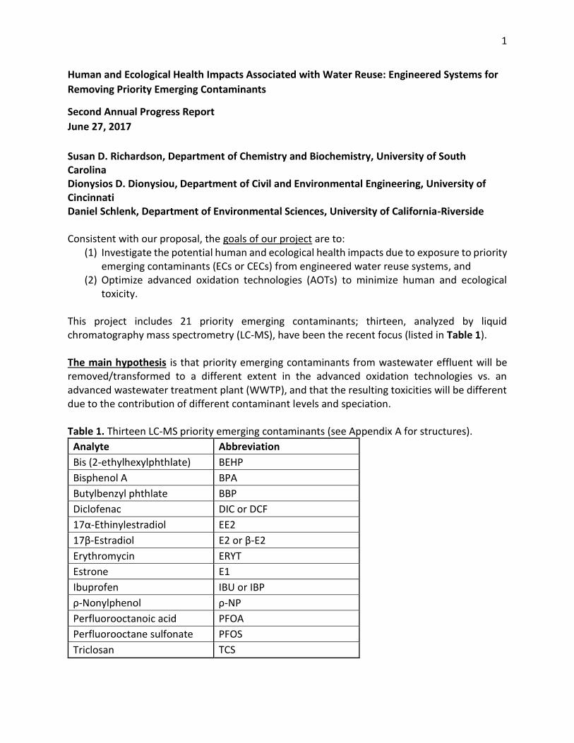
Second Annual Progress Report June 27, 2017 Susan D. Richardson, Department of Chemistry and Biochemistry, University of South Carolina Dionysios D. Dionysiou, Department of Civil and Environmental Engineering, University of Cincinnati Daniel Schlenk, Department of Environmental Sciences, University of California-Riverside Consistent with our proposal, the goals of our project are to:

(1) Investigate the potential human and ecological health impacts due to exposure to priority emerging contaminants (ECs or CECs) from engineered water reuse systems, and

(2) Optimize advanced oxidation technologies (AOTs) to minimize human and ecological toxicity.

This project includes 21 priority emerging contaminants; thirteen, analyzed by liquid chromatography mass spectrometry (LC-MS), have been the recent focus (listed in Table 1). The main hypothesis is that priority emerging contaminants from wastewater effluent will be removed/transformed to a different extent in the advanced oxidation technologies vs. an advanced wastewater treatment plant (WWTP), and that the resulting toxicities will be different due to the contribution of different contaminant levels and speciation. Table 1. Thirteen LC-MS priority emerging contaminants (see Appendix A for structures).

Analyte Abbreviation Bis (2-ethylhexylphthlate) BEHP Bisphenol A BPA Butylbenzyl phthlate BBP Diclofenac DIC or DCF 17α-Ethinylestradiol EE2 17β-Estradiol E2 or β-E2 Erythromycin ERYT Estrone E1 Ibuprofen IBU or IBP ρ-Nonylphenol ρ-NP Perfluorooctanoic acid PFOA Perfluorooctane sulfonate PFOS Triclosan TCS

2

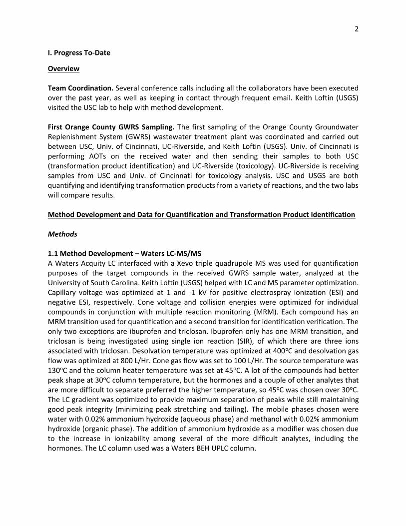
I. Progress To-Date

Overview

Team Coordination. Several conference calls including all the collaborators have been executed over the past year, as well as keeping in contact through frequent email. Keith Loftin (USGS) visited the USC lab to help with method development.

First Orange County GWRS Sampling. The first sampling of the Orange County Groundwater Replenishment System (GWRS) wastewater treatment plant was coordinated and carried out between USC, Univ. of Cincinnati, UC-Riverside, and Keith Loftin (USGS). Univ. of Cincinnati is performing AOTs on the received water and then sending their samples to both USC (transformation product identification) and UC-Riverside (toxicology). UC-Riverside is receiving samples from USC and Univ. of Cincinnati for toxicology analysis. USC and USGS are both quantifying and identifying transformation products from a variety of reactions, and the two labs will compare results.

Method Development and Data for Quantification and Transformation Product Identification Methods

1.1 Method Development – Waters LC-MS/MS A Waters Acquity LC interfaced with a Xevo triple quadrupole MS was used for quantification purposes of the target compounds in the received GWRS sample water, analyzed at the University of South Carolina. Keith Loftin (USGS) helped with LC and MS parameter optimization. Capillary voltage was optimized at 1 and -1 kV for positive electrospray ionization (ESI) and negative ESI, respectively. Cone voltage and collision energies were optimized for individual compounds in conjunction with multiple reaction monitoring (MRM). Each compound has an MRM transition used for quantification and a second transition for identification verification. The only two exceptions are ibuprofen and triclosan. Ibuprofen only has one MRM transition, and triclosan is being investigated using single ion reaction (SIR), of which there are three ions associated with triclosan. Desolvation temperature was optimized at 400oC and desolvation gas flow was optimized at 800 L/Hr. Cone gas flow was set to 100 L/Hr. The source temperature was 130oC and the column heater temperature was set at 45oC. A lot of the compounds had better peak shape at 30oC column temperature, but the hormones and a couple of other analytes that are more difficult to separate preferred the higher temperature, so 45oC was chosen over 30oC. The LC gradient was optimized to provide maximum separation of peaks while still maintaining good peak integrity (minimizing peak stretching and tailing). The mobile phases chosen were water with 0.02% ammonium hydroxide (aqueous phase) and methanol with 0.02% ammonium hydroxide (organic phase). The addition of ammonium hydroxide as a modifier was chosen due to the increase in ionizability among several of the more difficult analytes, including the hormones. The LC column used was a Waters BEH UPLC column.

3

1.2 Spiked Recoveries A solid phase extraction (SPE) method that had been developed previously was used for spiked recoveries and for extraction of the first round of GWRS samples. However, further optimization is being currently investigated to improve concentration factor and recovery. Water samples (100 mL of local treated wastewater effluent each) were acidified to pH 3 with sulfuric acid and then vacuum filtered through a 0.45 µm HVLP filter. The acidified, filtered water was then loaded onto conditioned Oasis HLB SPE cartridges and eluted with 15 mL of a 50:50 methanol/acetone solution. The 15 mL samples were blown down by nitrogen (in a TurboVap) to 1 mL. The samples were further diluted in a 3:7 dilution (300 µL sample and 700 µL high purity water) and then injected onto the instrument (Waters LC-MS mentioned previously). Spiked recoveries were analyzed using both an internal calibration curve and standard addition to compare the two methods. In order to further optimize the SPE method and improve recovery, several experiments were performed to investigate ways to increase concentration factor (see Table 2 in the data and results section). In the first test, triplicate wastewater samples were spiked, acidified, filtered, loaded on SPE cartridges, eluted with 15 mL (50:50 MeOH/acetone), blown down to 1 mL under nitrogen and further diluted in a 3:7 dilution as above. A wastewater blank was also treated the same way excepting the pre-filtration spike. Instead, the wastewater blank was separated into three samples after elution and dilution, and a low and high spike were added to two of them for use in standard addition. A spiked Milli-Q water sample was also done in conjunction with the wastewater samples. In the second test, triplicate wastewater samples were spiked, acidified, filtered, loaded on SPE cartridges, eluted with 15 mL (50:50 MeOH/acetone), blown down to 0.5 mL, and further diluted in a 2:8 dilution (200 µL sample and 800 µL aqueous internal standard solution). A wastewater blank with a low post-SPE spike for standard addition was also analyzed, as was a spiked Milli-Q water sample. In the third test, triplicate wastewater samples were spiked, acidified, filtered, loaded on SPE cartridges, eluted with 15 mL (50:50 MeOH/acetone), blown down to dryness under nitrogen, and reconstituted in 400 µL of aqueous internal standard solution. A wastewater blank with a low post-SPE spike for standard addition was also analyzed, as was a spiked Milli-Q water sample. 1.3 Quantification The first Orange County GWRS sampling event was in April and included five different water types plus travel blanks. These water types were secondary effluent, microfiltration, reverse osmosis, UV advanced oxidation, and Santa Ana River water. Samples were collected in both Teflon bottles and HDPE (high density polyethylene) bottles. The first four water types are all from the GWRS treatment plant, at different points in the advanced wastewater treatment process. The Santa Ana River water, which is primarily wastewater effluent, was obtained for comparison. Samples were 100 mL of water, acidifed and filtered as above and loaded on SPE cartridges. The elution, dilution, and injection procedure was also the same as above, with quantification data analyzed via both internal calibration curve and standard addition. Standard addition was done using a high spike and a low spike. Travel blanks were analyzed the same way. PFOA and PFOS, along with other perfluoroalkyl compounds, were quantified using EPA standard operating procedure EMAB-114-0 by Mark Strynar at the Research Triangle Park EPA lab in North Carolina.

4

Perfluoroalkyl compounds were quantified from the samples collected in HDPE bottles while the other compounds were quantified from the samples collected in Teflon bottles. 1.4 Transformation Product Identification Chlorination and chlorination/bromination reactions were carried out on each of the five water types and the travel blank. For chlorination reactions, sodium hypochlorite (NaOCl) was added at an estimated pre-determined molar ratio of 1:20 analyte:chlorine and the samples were put on a shaker for 30 minutes to ensure complete mixing and then allowed to react for 48 hours at room temperature. For chlorination/bromination reactions, sodium bromide was added before NaOCl and then shaken and allowed to react the same as the chlorination reactions. When the reactions were finished, the samples were acidified, filtered, and loaded onto SPE cartridges as before. Cartridges were eluted with 15 mL of a 50:50 methanol/acetone solution and blown to dryness under nitrogen. The samples were reconstituted in 400 µL of aqueous internal standard solution and injected on the instrument. Transformation products are in the process of being identified using an Agilent quadrupole time-of-flight mass spectrometer. 1.5 Perfluoroalkyl Compounds PFOA and PFOS are the two perfluoroalkyl compounds (PFAS’s) included in our list of priority emerging contaminants, however the EPA method used enabled quantification of several more perfluoroalkyl compounds in addition to just PFOA and PFOS. Samples for PFAS analysis were collected in HDPE bottles to avoid Teflon leachate contamination. EPA standard operating procedure (SOP) EMAB-113-0 was used for sampling and modified EPA SOP EMAB-114-0 was used to quantify PFAS’s. The list of compounds analyzed this way can be seen in Table 5 in the data and results section.

5

Data and Results 2.1. Spiked Recoveries Table 2. Spiked recoveries (%) of the three concentration factor optimization experiments. Spiked recoveries were done in local treated wastewater effluent. DW = ultra pure water (Milli-Q water) and WW = wastewater effluent. FC = concentration factor. ** denotes that test 3 had some injection troubles, most likely due to the small reconstitution volume.

TEST 1 (FC= 30x)

TEST 2 (FC=40x)

Test 3 (FC=250x)

DW WW DW WW DW WW 73 23 34 31 ** ** 9 7 8 13 ** ** 3 0 4 0 ** **

116 46 31 54 ** ** 162 84 168 51* ** ** 163 78 163 89 ** ** 82 48 54 54 ** ** 41 13 9 40 ** **

812 376 819 424 ** ** 333 150 347 177 ** ** 285 135 221 148 ** ** 89 33 120 58 ** ** 37 25 30 39 ** **

2.2. Quantification Thirteen emerging contaminants were quantified by internal calibration curve and by standard addition. The current extraction method used needs modification to increase concentration factor.

6

Table 3. Concentrations of priority emerging contaminants in the GWRS water samples. Concentrations are in ppt (ng/L). The levels in the blank were higher than expected due to contamination, so the concentrations reported below are those that were higher than the travel blank. The travel blank concentrations were subtracted from the sample concentrations and the differences were reported here. LOD is limit of detection and LOQ is limit of quantification. The levels reported here were all above LOD and LOQ before subtracting the travel blank concentration.

Analyte Secondary Effluent Microfiltration Reverse

Osmosis UV AOP Santa Ana River LOD LOQ

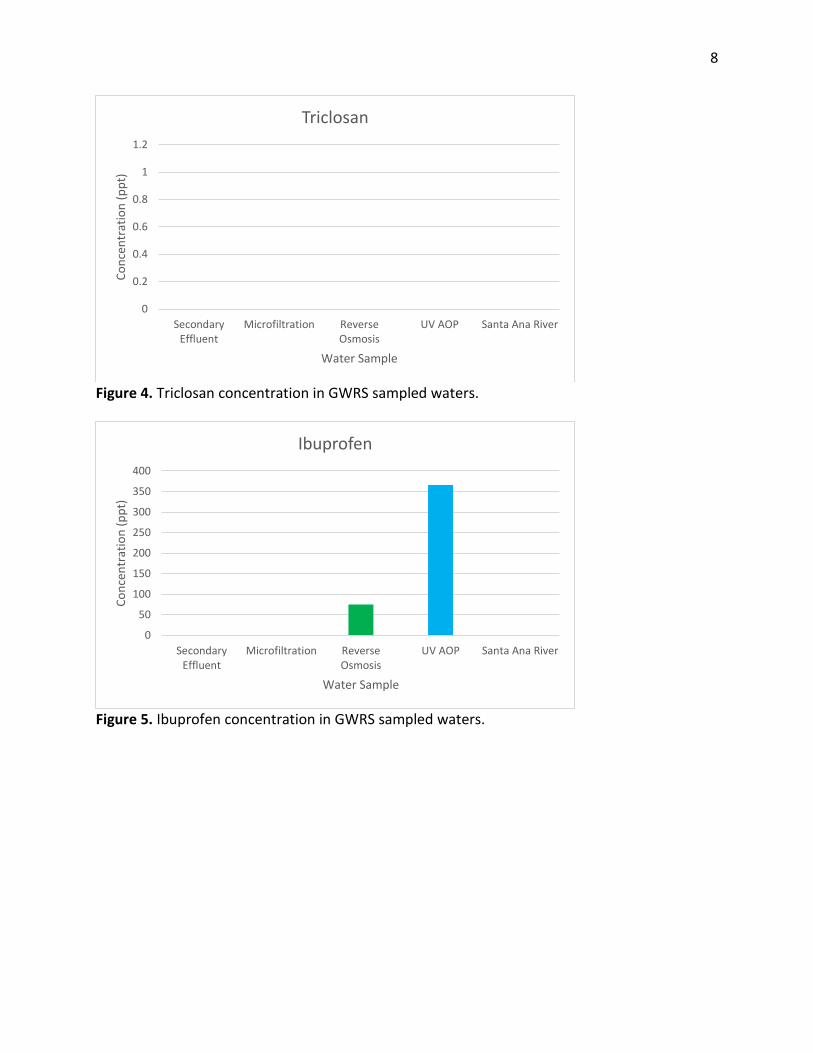
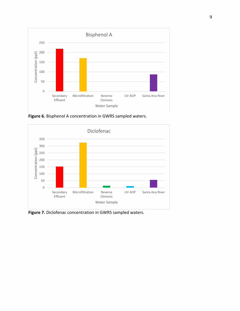
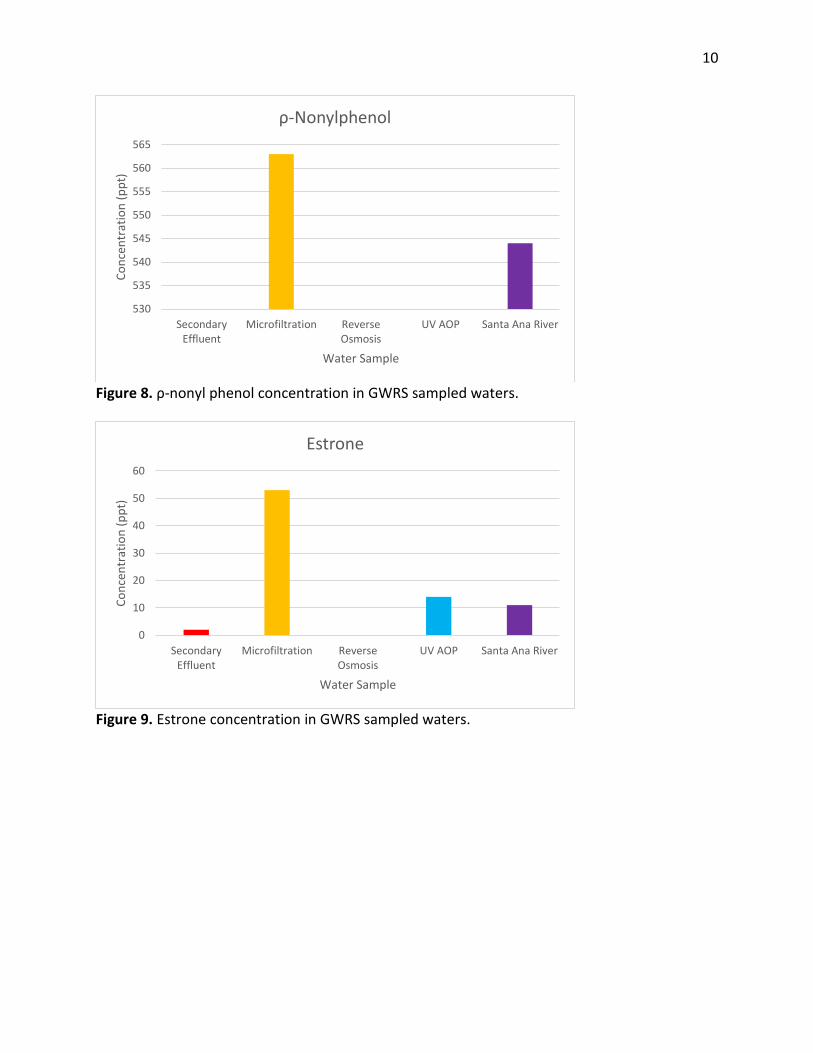
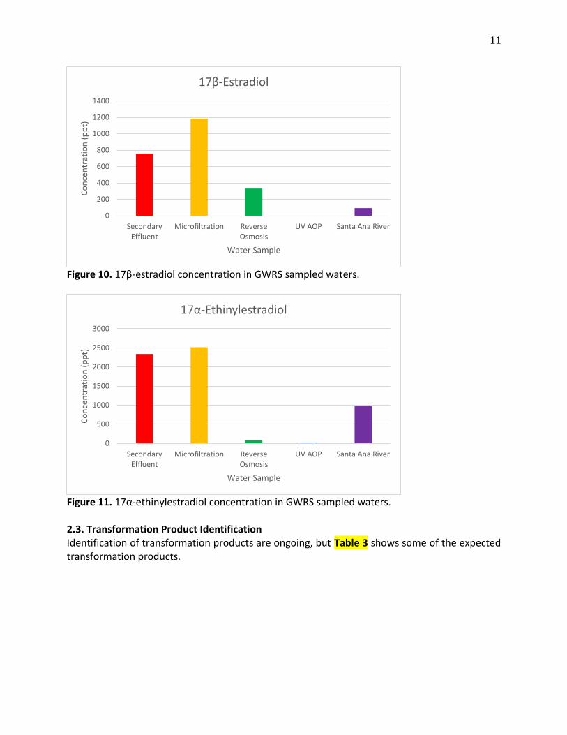
BBP 8 25 246 56 186 BEHP 62 28 196 181 603 ERYT 4 27 60 68 227 TCS 998 3328 IBU 75 366 268 892 BPA 219 171 87 75 250 DIC 152 325 14 11 56 25 83 NP 563 544 255 850 E1 2 53 14 11 386 1286

β-E2 758 1183 331 93 489 1659 EE2 2340 2516 79 16 976 249 829

Figure 1. Butyl benzyl phthalate concentration in GWRS sampled waters.

0

50

100

150

200

250

300

SecondaryEffluent

Microfiltration ReverseOsmosis

UV AOP Santa Ana River

Conc

entr

atio

n (p

pt)

Water Sample

Butyl Benzyl Phthalate

7

Figure 2. Bis (2-ethylhexyl) phthalate concentration in GWRS sampled waters.

Figure 3. Erythromycin concentration in GWRS sampled waters.

0

50

100

150

200

250

SecondaryEffluent



Conc

entr

atio

n (p

pt)

Water Sample

Bis (2-ethylhexyl) Phthalate

0

10

20

30

40

50

60

70

SecondaryEffluent



Conc

entr

atio

n (p

pt)

Water Sample

Erythromycin

8

Figure 4. Triclosan concentration in GWRS sampled waters.

Figure 5. Ibuprofen concentration in GWRS sampled waters.

0

0.2

0.4

0.6

0.8

1

1.2

SecondaryEffluent



Conc

entr

atio

n (p

pt)

Water Sample

Triclosan

0

50

100

150

200

250

300

350

400

SecondaryEffluent



Conc

entr

atio

n (p

pt)

Water Sample

Ibuprofen

9

Figure 6. Bisphenol A concentration in GWRS sampled waters.

Figure 7. Diclofenac concentration in GWRS sampled waters.

0

50

100

150

200

250

SecondaryEffluent



Conc

entr

atio

n (p

pt)

Water Sample

Bisphenol A

0

50

100

150

200

250

300

350

SecondaryEffluent



Conc

entr

atio

n (p

pt)

Water Sample

Diclofenac

10

Figure 8. ρ-nonyl phenol concentration in GWRS sampled waters.

Figure 9. Estrone concentration in GWRS sampled waters.

530

535

540

545

550

555

560

565

SecondaryEffluent



Conc

entr

atio

n (p

pt)

Water Sample

ρ-Nonylphenol

0

10

20

30

40

50

60

SecondaryEffluent



Conc

entr

atio

n (p

pt)

Water Sample

Estrone

11

Figure 10. 17β-estradiol concentration in GWRS sampled waters.

Figure 11. 17α-ethinylestradiol concentration in GWRS sampled waters. 2.3. Transformation Product Identification Identification of transformation products are ongoing, but Table 3 shows some of the expected transformation products.

0

200

400

600

800

1000

1200

1400

SecondaryEffluent



Conc

entr

atio

n (p

pt)

Water Sample

17β-Estradiol

0

500

1000

1500

2000

2500

3000

SecondaryEffluent



Conc

entr

atio

n (p

pt)

Water Sample

17α-Ethinylestradiol

12

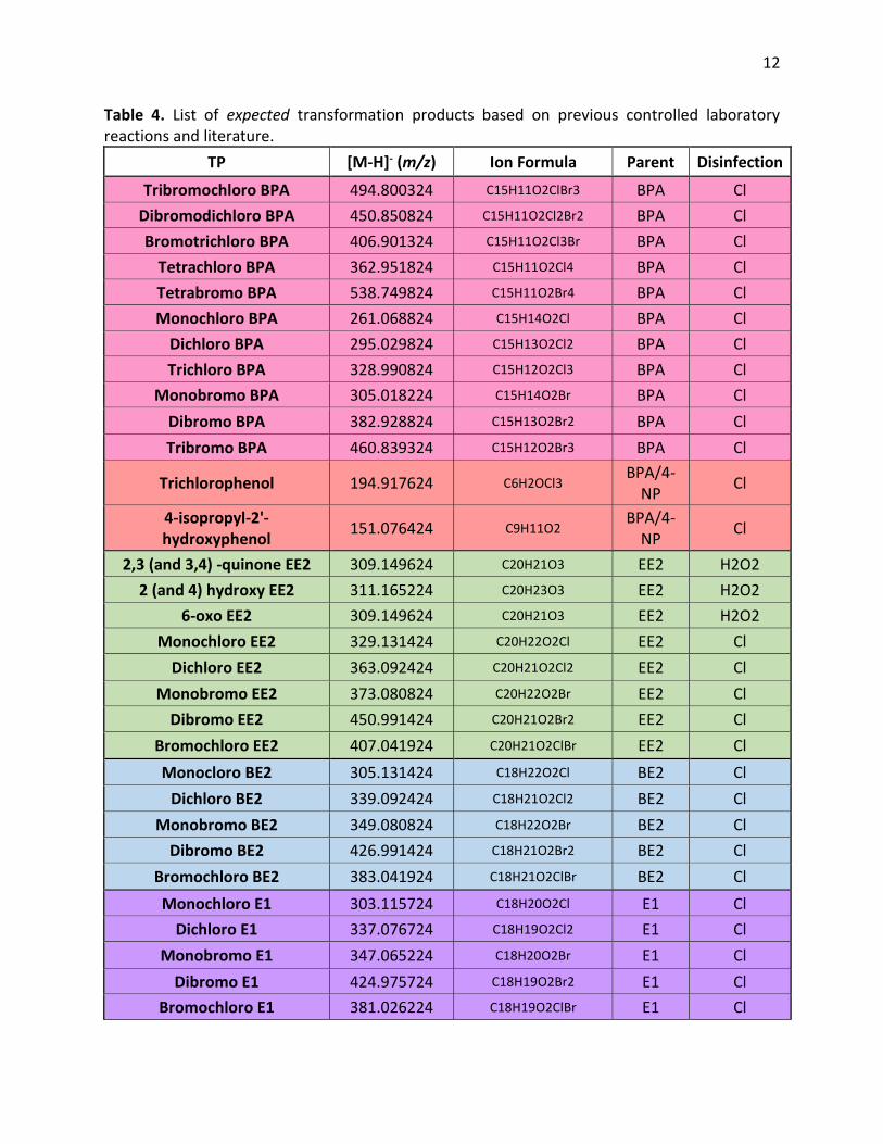
Table 4. List of expected transformation products based on previous controlled laboratory reactions and literature.

TP [M-H]- (m/z) Ion Formula Parent Disinfection Tribromochloro BPA 494.800324 C15H11O2ClBr3 BPA Cl

Dibromodichloro BPA 450.850824 C15H11O2Cl2Br2 BPA Cl Bromotrichloro BPA 406.901324 C15H11O2Cl3Br BPA Cl

Tetrachloro BPA 362.951824 C15H11O2Cl4 BPA Cl Tetrabromo BPA 538.749824 C15H11O2Br4 BPA Cl Monochloro BPA 261.068824 C15H14O2Cl BPA Cl

Dichloro BPA 295.029824 C15H13O2Cl2 BPA Cl Trichloro BPA 328.990824 C15H12O2Cl3 BPA Cl

Monobromo BPA 305.018224 C15H14O2Br BPA Cl Dibromo BPA 382.928824 C15H13O2Br2 BPA Cl Tribromo BPA 460.839324 C15H12O2Br3 BPA Cl

Trichlorophenol 194.917624 C6H2OCl3 BPA/4-

NP Cl

4-isopropyl-2'-hydroxyphenol 151.076424 C9H11O2

BPA/4-NP Cl

2,3 (and 3,4) -quinone EE2 309.149624 C20H21O3 EE2 H2O2 2 (and 4) hydroxy EE2 311.165224 C20H23O3 EE2 H2O2

6-oxo EE2 309.149624 C20H21O3 EE2 H2O2 Monochloro EE2 329.131424 C20H22O2Cl EE2 Cl

Dichloro EE2 363.092424 C20H21O2Cl2 EE2 Cl Monobromo EE2 373.080824 C20H22O2Br EE2 Cl

Dibromo EE2 450.991424 C20H21O2Br2 EE2 Cl Bromochloro EE2 407.041924 C20H21O2ClBr EE2 Cl Monocloro BE2 305.131424 C18H22O2Cl BE2 Cl

Dichloro BE2 339.092424 C18H21O2Cl2 BE2 Cl Monobromo BE2 349.080824 C18H22O2Br BE2 Cl

Dibromo BE2 426.991424 C18H21O2Br2 BE2 Cl Bromochloro BE2 383.041924 C18H21O2ClBr BE2 Cl Monochloro E1 303.115724 C18H20O2Cl E1 Cl

Dichloro E1 337.076724 C18H19O2Cl2 E1 Cl Monobromo E1 347.065224 C18H20O2Br E1 Cl

Dibromo E1 424.975724 C18H19O2Br2 E1 Cl Bromochloro E1 381.026224 C18H19O2ClBr E1 Cl

13

Hexachloro-oxo-E1 524.936924 C18H19O5Cl6 E1 Cl Dichlorophenol 160.956624 C6H3OCl2 TCS Cl, UV

2,8-DCDD 250.967224 C12H5O2Cl2 TCS Cl, UV Methyl triclosan 300.959524 C13H8O2Cl3 TCS Cl, UV

Chloroform 116.907124 CHCl3 TCS Cl, UV 2-Chloro-4-NP 253.136424 C15H22OCl 4-NP Cl

2,6-Dichloro-4-NP 287.097524 C15H21OCl2 4-NP Cl 4-isobutyl-2-hydroxyphenol 165.092124 C10H13O2 4-NP Cl

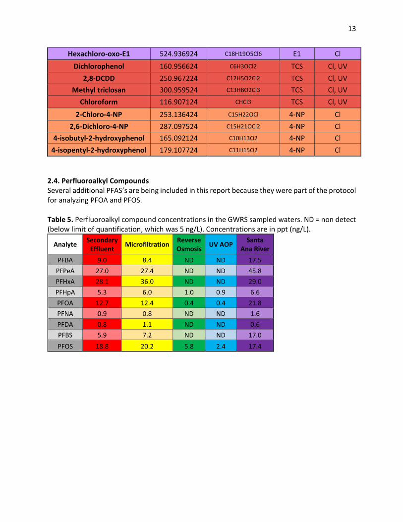
4-isopentyl-2-hydroxyphenol 179.107724 C11H15O2 4-NP Cl 2.4. Perfluoroalkyl Compounds Several additional PFAS’s are being included in this report because they were part of the protocol for analyzing PFOA and PFOS. Table 5. Perfluoroalkyl compound concentrations in the GWRS sampled waters. ND = non detect (below limit of quantification, which was 5 ng/L). Concentrations are in ppt (ng/L).

Analyte Secondary Effluent Microfiltration Reverse

Osmosis UV AOP Santa Ana River

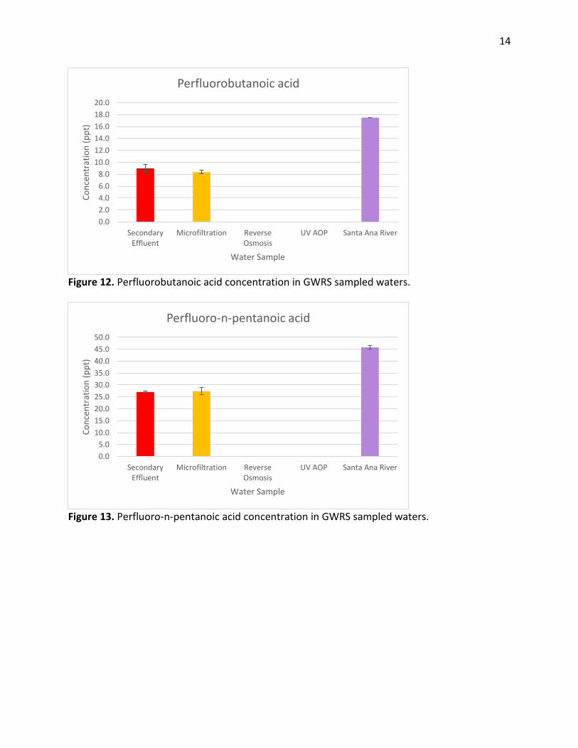
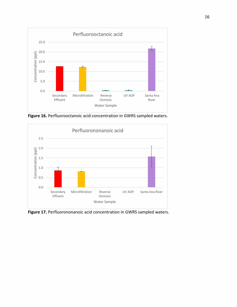
PFBA 9.0 8.4 ND ND 17.5 PFPeA 27.0 27.4 ND ND 45.8 PFHxA 28.1 36.0 ND ND 29.0 PFHpA 5.3 6.0 1.0 0.9 6.6 PFOA 12.7 12.4 0.4 0.4 21.8 PFNA 0.9 0.8 ND ND 1.6 PFDA 0.8 1.1 ND ND 0.6 PFBS 5.9 7.2 ND ND 17.0 PFOS 18.8 20.2 5.8 2.4 17.4

14

Figure 12. Perfluorobutanoic acid concentration in GWRS sampled waters.

Figure 13. Perfluoro-n-pentanoic acid concentration in GWRS sampled waters.

0.02.04.06.08.0

10.012.014.016.018.020.0

SecondaryEffluent



Conc

entr

atio

n (p

pt)

Water Sample

Perfluorobutanoic acid

0.05.0

10.015.020.025.030.035.040.045.050.0

SecondaryEffluent



Conc

entr

atio

n (p

pt)

Water Sample

Perfluoro-n-pentanoic acid

15

Figure 14. Perfluorohexanoic acid concentration in GWRS sampled waters.

Figure 15. Perfluoroheptanoic acid concentration in GWRS sampled waters.

0.0

5.0

10.0

15.0

20.0

25.0

30.0

35.0

40.0

SecondaryEffluent



Conc

entr

atio

n (p

pt)

Water Sample

Perfluorohexanoic acid

0.0

1.0

2.0

3.0

4.0

5.0

6.0

7.0

8.0

SecondaryEffluent



Conc

entr

atio

n (p

pt)

Water Sample

Perfluoroheptanoic acid

16

Figure 16. Perfluorooctanoic acid concentration in GWRS sampled waters.

Figure 17. Perfluorononanoic acid concentration in GWRS sampled waters.

0.0

5.0

10.0

15.0

20.0

25.0

SecondaryEffluent


UV AOP Santa AnaRiver

Conc

entr

atio

n (p

pt)

Water Sample

Perfluorooctanoic acid

0.0

0.5

1.0

1.5

2.0

2.5

SecondaryEffluent



Conc

entr

atio

n (p

pt)

Water Sample

Perfluorononanoic acid

17

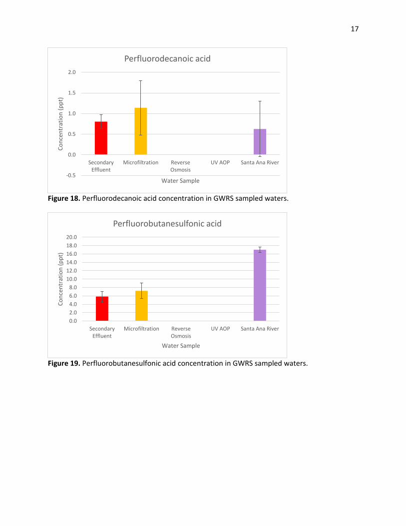
Figure 18. Perfluorodecanoic acid concentration in GWRS sampled waters.

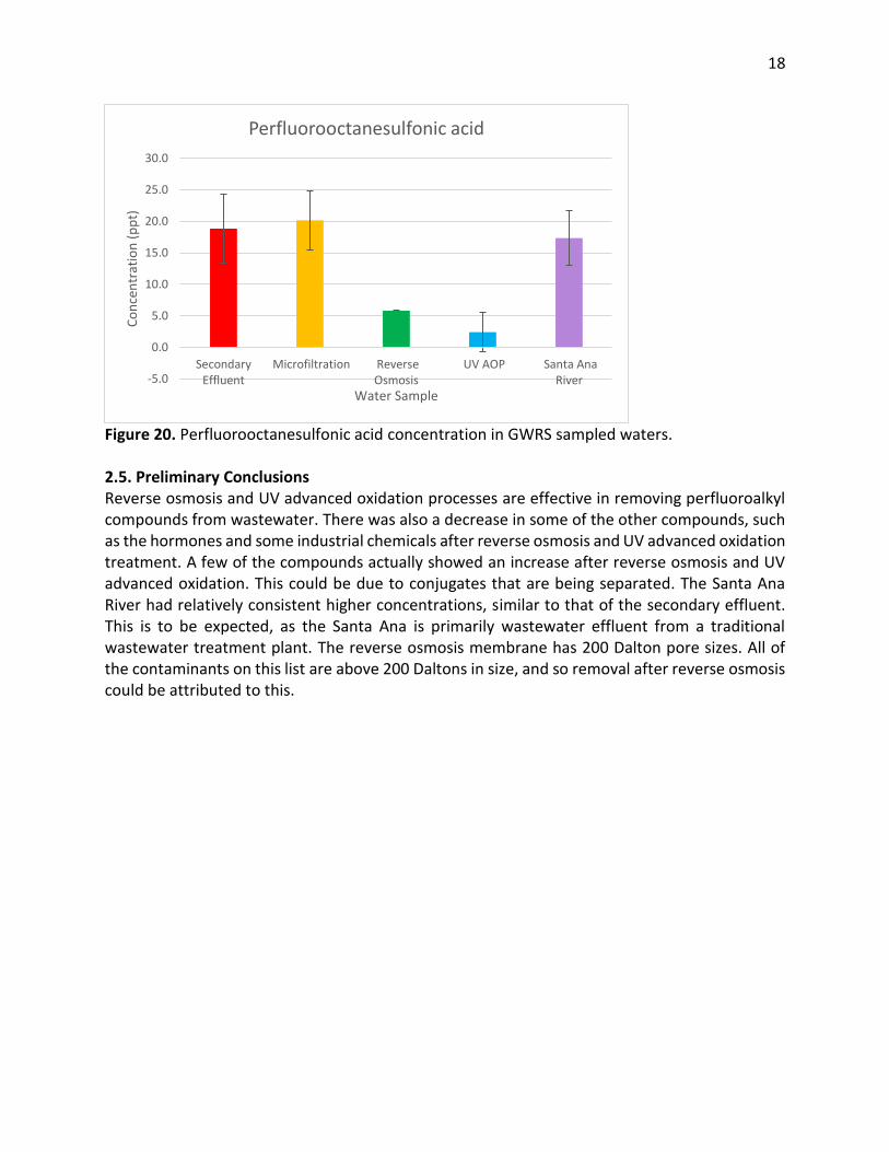
Figure 19. Perfluorobutanesulfonic acid concentration in GWRS sampled waters.

-0.5

0.0

0.5

1.0

1.5

2.0

SecondaryEffluent



Conc

entr

atio

n (p

pt)

Water Sample

Perfluorodecanoic acid

0.02.04.06.08.0

10.012.014.016.018.020.0

SecondaryEffluent



Conc

entr

atio

n (p

pt)

Water Sample

Perfluorobutanesulfonic acid

18

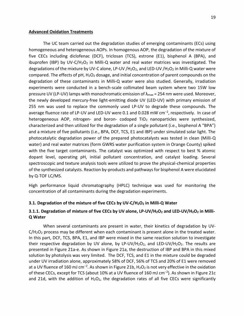
Figure 20. Perfluorooctanesulfonic acid concentration in GWRS sampled waters. 2.5. Preliminary Conclusions Reverse osmosis and UV advanced oxidation processes are effective in removing perfluoroalkyl compounds from wastewater. There was also a decrease in some of the other compounds, such as the hormones and some industrial chemicals after reverse osmosis and UV advanced oxidation treatment. A few of the compounds actually showed an increase after reverse osmosis and UV advanced oxidation. This could be due to conjugates that are being separated. The Santa Ana River had relatively consistent higher concentrations, similar to that of the secondary effluent. This is to be expected, as the Santa Ana is primarily wastewater effluent from a traditional wastewater treatment plant. The reverse osmosis membrane has 200 Dalton pore sizes. All of the contaminants on this list are above 200 Daltons in size, and so removal after reverse osmosis could be attributed to this.

-5.0

0.0

5.0

10.0

15.0

20.0

25.0

30.0

SecondaryEffluent


UV AOP Santa AnaRiver

Conc

entr

atio

n (p

pt)

Water Sample

Perfluorooctanesulfonic acid

19

Advanced Oxidation Treatments

The UC team carried out the degradation studies of emerging contaminants (ECs) using homogeneous and heterogeneous AOPs. In homogenous AOP, the degradation of the mixture of five CECs including diclofenac (DCF), triclosan (TCS), estrone (E1), bisphenol A (BPA), and ibuprofen (IBP) by UV-C/H2O2 in Milli-Q water and real water matrices was investigated. The degradations of the mixture by UV-C alone, LP-UV /H2O2, and LED-UV /H2O2 in Milli-Q water were compared. The effects of pH, H2O2 dosage, and initial concentration of parent compounds on the degradation of these contaminants in Milli-Q water were also studied. Generally, irradiation experiments were conducted in a bench-scale collimated beam system where two 15W low pressure UV (LP-UV) lamps with monochromatic emission of λmax = 254 nm were used. Moreover, the newly developed mercury-free light-emitting diode UV (LED-UV) with primary emission of 255 nm was used to replace the commonly used LP-UV to degrade these compounds. The average fluence rate of LP-UV and LED-UV were 0.1 and 0.028 mW cm−2, respectively. In case of heterogeneous AOP, nitrogen- and boron- codoped TiO2 nanoparticles were synthesized, characterized and then utilized for the degradation of a single pollutant (i.e., bisphenol A “BPA”) and a mixture of five pollutants (i.e., BPA, DCF, TCS, E1 and IBP) under simulated solar light. The photocatalytic degradation power of the prepared photocatalysts was tested in clean (Milli-Q water) and real water matrices (form GWRS water purification system in Orange County) spiked with the five target contaminants. The catalyst was optimized with respect to best % atomic dopant level, operating pH, initial pollutant concentration, and catalyst loading. Several spectroscopic and texture analysis tools were utilized to prove the physical-chemical properties of the synthesized catalysts. Reaction by-products and pathways for bisphenol A were elucidated by Q-TOF LC/MS.

High performance liquid chromatography (HPLC) technique was used for monitoring the concentration of all contaminants during the degradation experiments. 3.1. Degradation of the mixture of five CECs by UV-C/H2O2 in Milli-Q Water

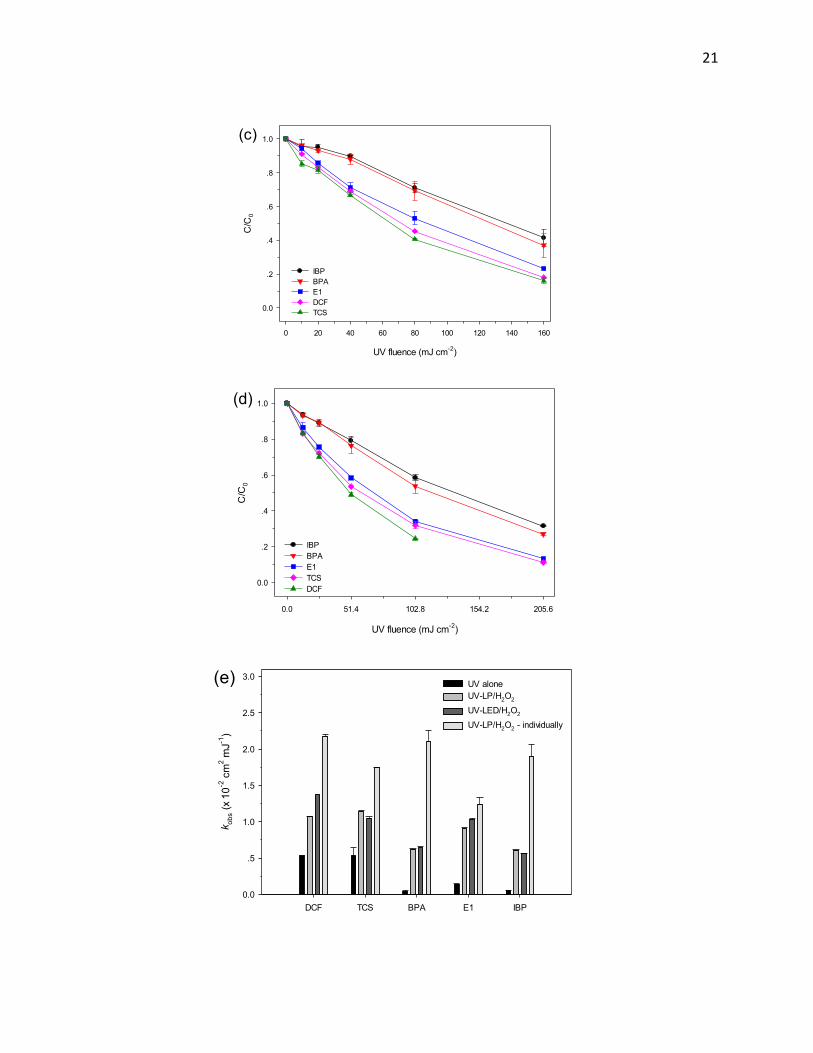
3.1.1. Degradation of mixture of five CECs by UV alone, LP-UV/H2O2 and LED-UV/H2O2 in Milli-Q Water

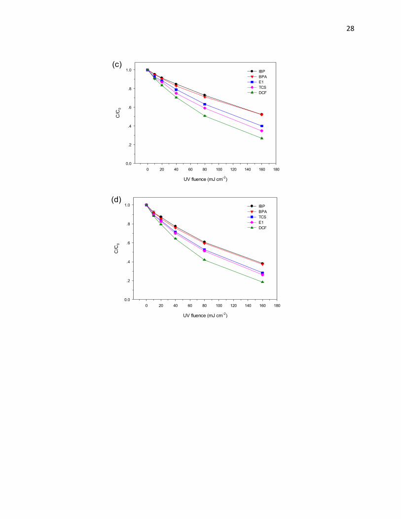
When several contaminants are present in water, their kinetics of degradation by UV-C/H2O2 process may be different when each contaminant is present alone in the treated water. In this part, DCF, TCS, BPA, E1, and IBP were mixed in the same reaction solution to investigate their respective degradation by UV alone, by LP-UV/H2O2, and LED-UV/H2O2. The results are presented in Figure 21a-e. As shown in Figure 21a, the destruction of IBP and BPA in this mixed solution by photolysis was very limited. The DCF, TCS, and E1 in the mixture could be degraded under UV irradiation alone, approximately 58% of DCF, 56% of TCS and 20% of E1 were removed at a UV fluence of 160 mJ cm−2. As shown in Figure 21b, H2O2 is not very effective in the oxidation of these CECs, except for TCS (about 10% at a UV fluence of 160 mJ cm−2). As shown in Figure 21c and 21d, with the addition of H2O2, the degradation rates of all five CECs were significantly

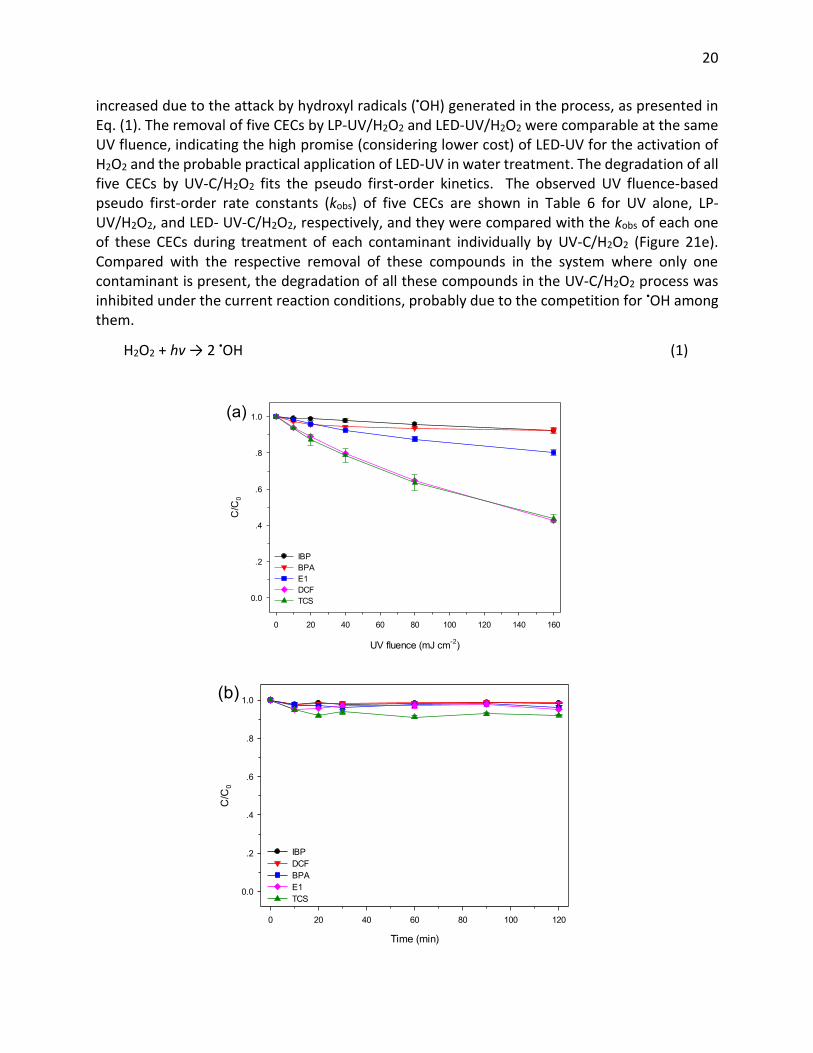
20

increased due to the attack by hydroxyl radicals (•OH) generated in the process, as presented in Eq. (1). The removal of five CECs by LP-UV/H2O2 and LED-UV/H2O2 were comparable at the same UV fluence, indicating the high promise (considering lower cost) of LED-UV for the activation of H2O2 and the probable practical application of LED-UV in water treatment. The degradation of all five CECs by UV-C/H2O2 fits the pseudo first-order kinetics. The observed UV fluence-based pseudo first-order rate constants (kobs) of five CECs are shown in Table 6 for UV alone, LP-UV/H2O2, and LED- UV-C/H2O2, respectively, and they were compared with the kobs of each one of these CECs during treatment of each contaminant individually by UV-C/H2O2 (Figure 21e). Compared with the respective removal of these compounds in the system where only one contaminant is present, the degradation of all these compounds in the UV-C/H2O2 process was inhibited under the current reaction conditions, probably due to the competition for •OH among them.

H2O2 + hv → 2 •OH (1)

UV fluence (mJ cm-2)

0 20 40 60 80 100 120 140 160

C/C

0

0.0

.2

.4

.6

.8

1.0

IBP BPA E1 DCF TCS

(a)

Time (min)

0 20 40 60 80 100 120

C/C

0

0.0

.2

.4

.6

.8

1.0

IBP DCF BPA E1 TCS

(b)

21


0 20 40 60 80 100 120 140 160

C/C

0

0.0

.2

.4

.6

.8

1.0

IBP BPA E1 DCF TCS

(c)


0.0 51.4 102.8 154.2 205.6

C/C

0

0.0

.2

.4

.6

.8

1.0

IBP BPA E1 TCS DCF

(d)

DCF TCS BPA E1 IBP

k obs

(x 1

0-2 c

m2 m

J-1)

0.0

.5

1.0

1.5

2.0

2.5

3.0UV alone UV-LP/H2O2 UV-LED/H2O2 UV-LP/H2O2 - individually

(e)

22

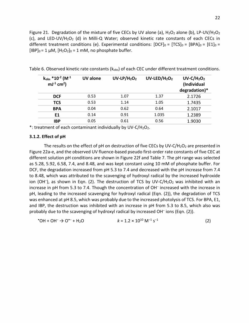
Figure 21. Degradation of the mixture of five CECs by UV alone (a), H2O2 alone (b), LP-UV/H2O2 (c), and LED-UV/H2O2 (d) in Milli-Q Water; observed kinetic rate constants of each CECs in different treatment conditions (e). Experimental conditions: [DCF]0 = [TCS]0 = [BPA]0 = [E1]0 = [IBP]0 = 1 µM, [H2O2]0 = 1 mM, no phosphate buffer.

Table 6. Observed kinetic rate constants (kobs) of each CEC under different treatment conditions.

kobs *10-2 (M-1 mJ-1 cm2)

UV alone UV-LP/H2O2

UV-LED/H2O2

UV-C/H2O2 (Individual

degradation)* DCF 0.53 1.07 1.37 2.1726 TCS 0.53 1.14 1.05 1.7435 BPA 0.04 0.62 0.64 2.1017 E1 0.14 0.91 1.035 1.2389 IBP 0.05 0.61 0.56 1.9030

*: treatment of each contaminant individually by UV-C/H2O2.

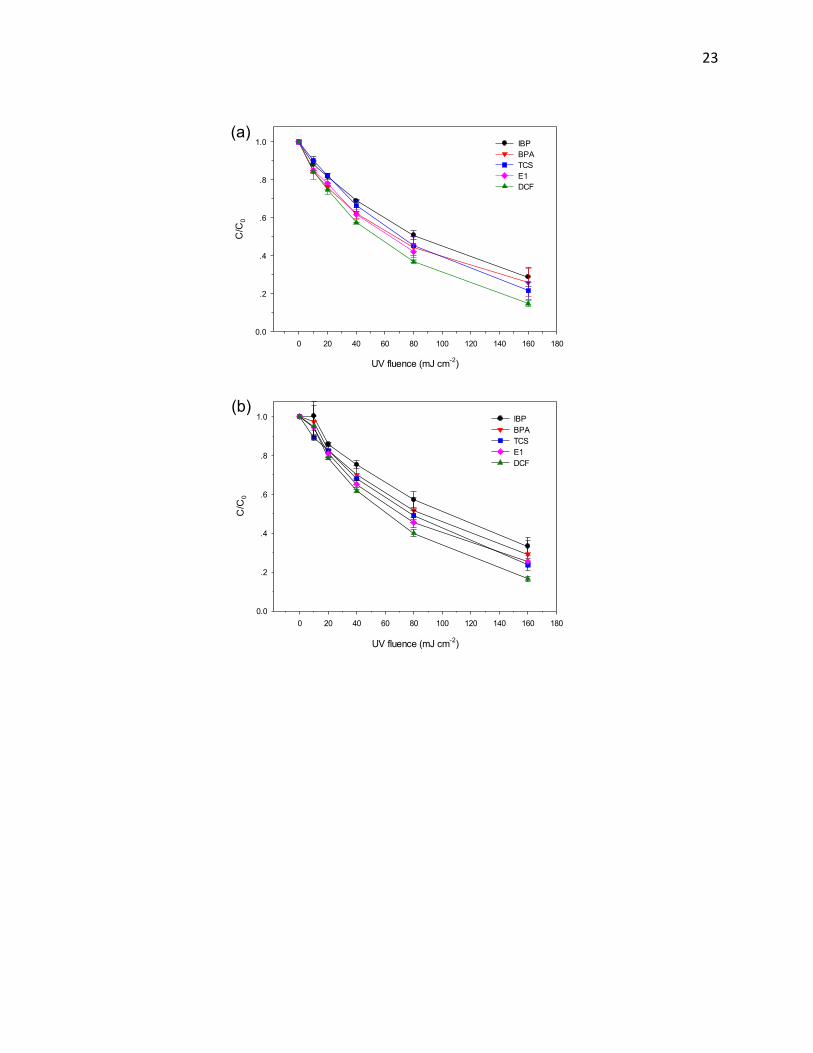
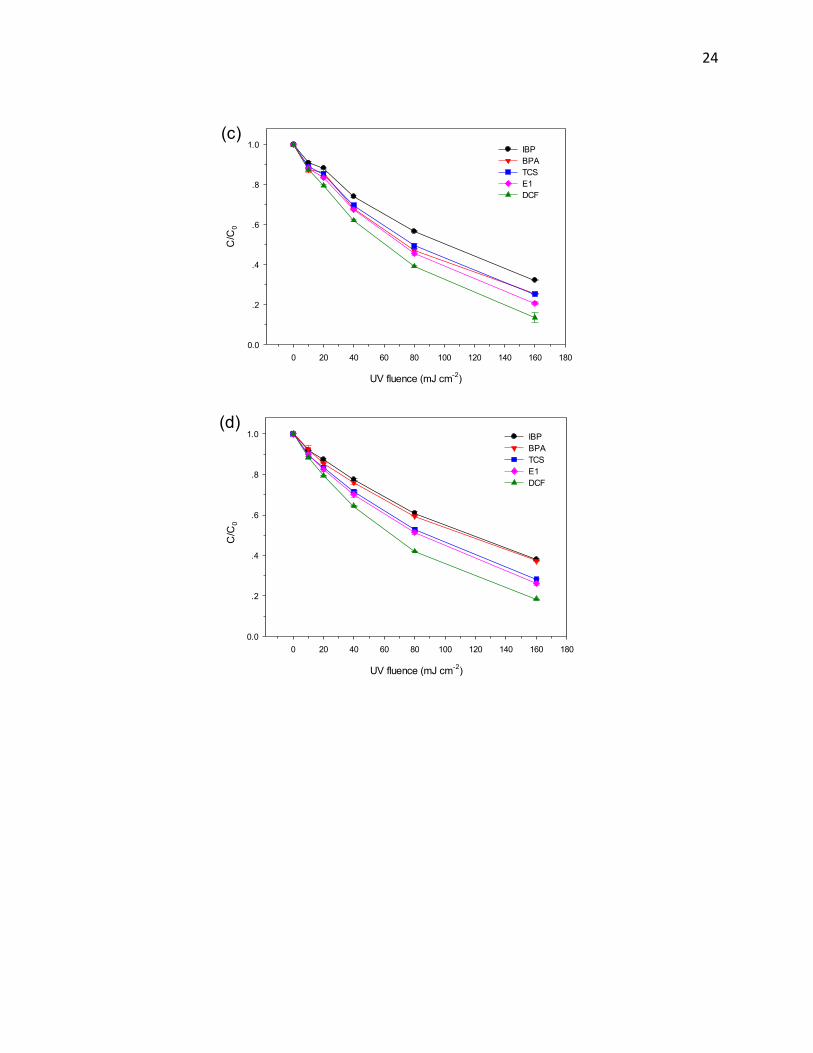
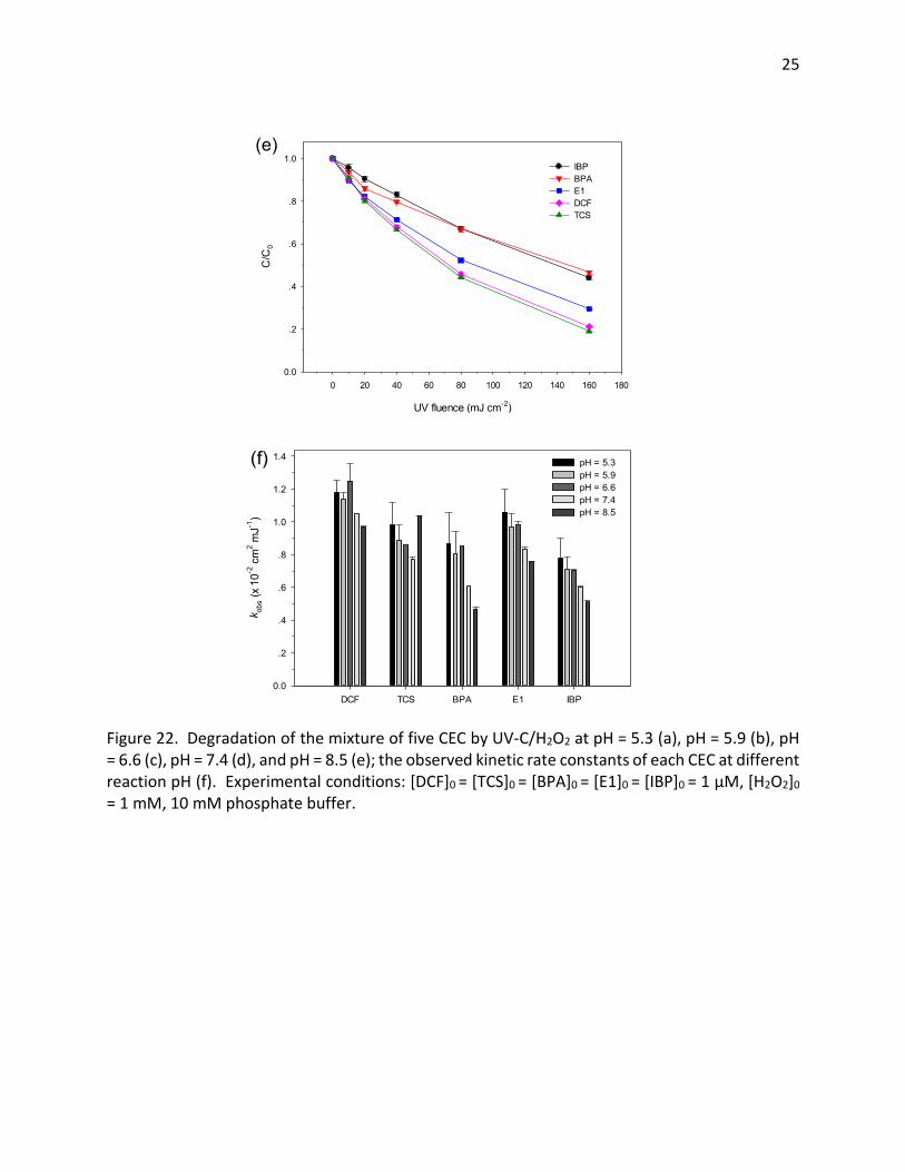
3.1.2. Effect of pH

The results on the effect of pH on destruction of five CECs by UV-C/H2O2 are presented in Figure 22a-e, and the observed UV fluence-based pseudo first-order rate constants of five CEC at different solution pH conditions are shown in Figure 22f and Table 7. The pH range was selected as 5.28, 5.92, 6.58, 7.4, and 8.48, and was kept constant using 10 mM of phosphate buffer. For DCF, the degradation increased from pH 5.3 to 7.4 and decreased with the pH increase from 7.4 to 8.48, which was attributed to the scavenging of hydroxyl radical by the increased hydroxide ion (OH−), as shown in Eqn. (2). The destruction of TCS by UV-C/H2O2 was inhibited with an increase in pH from 5.3 to 7.4. Though the concentration of OH− increased with the increase in pH, leading to the increased scavenging for hydroxyl radical (Eqn. (2)), the degradation of TCS was enhanced at pH 8.5, which was probably due to the increased photolysis of TCS. For BPA, E1, and IBP, the destruction was inhibited with an increase in pH from 5.3 to 8.5, which also was probably due to the scavenging of hydroxyl radical by increased OH− ions (Eqn. (2)).

•OH + OH− → O•− + H2O k = 1.2 × 1010 M−1 s−1 (2)

23


0 20 40 60 80 100 120 140 160 180

C/C

0

0.0

.2

.4

.6

.8

1.0 IBP BPA TCS E1 DCF

(a)


0 20 40 60 80 100 120 140 160 180

C/C

0

0.0

.2

.4

.6

.8


(b)

24


0 20 40 60 80 100 120 140 160 180

C/C

0

0.0

.2

.4

.6

.8


(c)


0 20 40 60 80 100 120 140 160 180

C/C

0

0.0

.2

.4

.6

.8


(d)

25


0 20 40 60 80 100 120 140 160 180

C/C

0

0.0

.2

.4

.6

.8

1.0IBP BPA E1 DCF TCS

(e)

DCF TCS BPA E1 IBP

k obs

(x 1

0- 2 c

m2 m

J- 1)

0.0

.2

.4

.6

.8

1.0

1.2

1.4 pH = 5.3 pH = 5.9 pH = 6.6 pH = 7.4 pH = 8.5

(f)

Figure 22. Degradation of the mixture of five CEC by UV-C/H2O2 at pH = 5.3 (a), pH = 5.9 (b), pH = 6.6 (c), pH = 7.4 (d), and pH = 8.5 (e); the observed kinetic rate constants of each CEC at different reaction pH (f). Experimental conditions: [DCF]0 = [TCS]0 = [BPA]0 = [E1]0 = [IBP]0 = 1 µM, [H2O2]0 = 1 mM, 10 mM phosphate buffer.

26

Table 7. Observed kinetic rate constants (kobs) of each CEC at different solution pH.

kobs *10-2 (M-

1 mJ-1 cm2)

pH = 5.3 pH = 5.9

pH = 6.6

pH = 7.4 pH = 8.5

DCF 1.18 1.14 1.25 1.05 0.97 TCS 0.98 0.89 0.86 0.775 1.035 BPA 0.865 0.805 0.85 0.61 0.465 E1 1.06 0.97 0.98 0.83 0.755 IBP 0.78 0.71 0.705 0.6 0.51

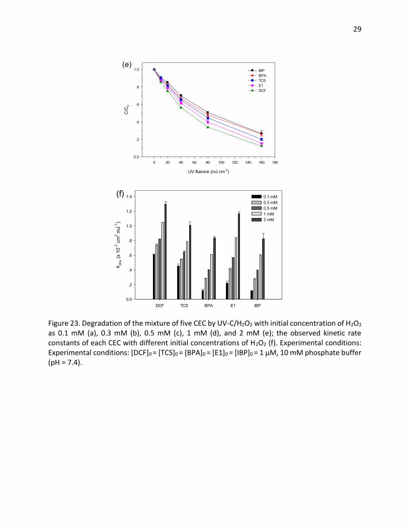
3.1.3. Effect of initial H2O2 dosage

Oxidant dosage is an important parameter in evaluating the applicability of UV-C/H2O2 process. Figure 23a-e describes the effect of initial H2O2 dosage on the degradation of five CEC. The observed UV fluence-based pseudo first-order rate constants of five CEC with different initial H2O2 dose is shown in Figure 23f and Table 8. The removal of each CEC increased with the increase of initial H2O2 concentration; however, there was no linear increase of kobs with the increase in H2O2 dose, which could probably result from the scavenging effect of the excess H2O2, specifically the competitive radical reactions (Eqs. (3)-(5)).

•OH + H2O2 → HO2• + H2O k = 2.7 × 107 M−1 s−1 (3) •OH + HO2• → O2 + H2O k = 6.6 × 109 M−1 s−1 (4) •OH + •OH → H2O2 k = 5.5 × 109 M−1 s−1 (5)

27


0 20 40 60 80 100 120 140 160 180

C/C

0

0.0

.2

.4

.6

.8

1.0 IBP BPA E1 TCS DCF

(a)


0 20 40 60 80 100 120 140 160 180

C/C

0

0.0

.2

.4

.6

.8

1.0 IBP BPAE1TCSDCF

(b)

28


0 20 40 60 80 100 120 140 160 180

C/C

0

0.0

.2

.4

.6

.8

1.0 IBPBPAE1TCSDCF

(c)


0 20 40 60 80 100 120 140 160 180

C/C

0

0.0

.2

.4

.6

.8


(d)

29


0 20 40 60 80 100 120 140 160 180

C/C

0

0.0

.2

.4

.6

.8

1.0 IBPBPATCSE1DCF

(e)

DCF TCS BPA E1 IBP

k obs

(x 1

0-2 c

m2 m

J-1)

0.0

.2

.4

.6

.8

1.0

1.2

1.4 0.1 mM 0.3 mM 0.5 mM 1 mM 2 mM

(f)

Figure 23. Degradation of the mixture of five CEC by UV-C/H2O2 with initial concentration of H2O2 as 0.1 mM (a), 0.3 mM (b), 0.5 mM (c), 1 mM (d), and 2 mM (e); the observed kinetic rate constants of each CEC with different initial concentrations of H2O2 (f). Experimental conditions: Experimental conditions: [DCF]0 = [TCS]0 = [BPA]0 = [E1]0 = [IBP]0 = 1 µM, 10 mM phosphate buffer (pH = 7.4).

30

Table 8. Observed kinetic rate constants (kobs) of each CECs with different initial concentrations of H2O2.

kobs *10-2 (M-

1 mJ-1 cm2)

0.1 mM 0.3 mM

0.5 mM

1 mM 2 mM

DCF 0.61 0.74 0.815 1.05 1.295 TCS 0.45 0.545 0.645 0.775 1.01 BPA 0.12 0.28 0.4 0.61 0.84 E1 0.22 0.415 0.565 0.83 1.165 IBP 0.12 0.275 0.4 0.6 0.825

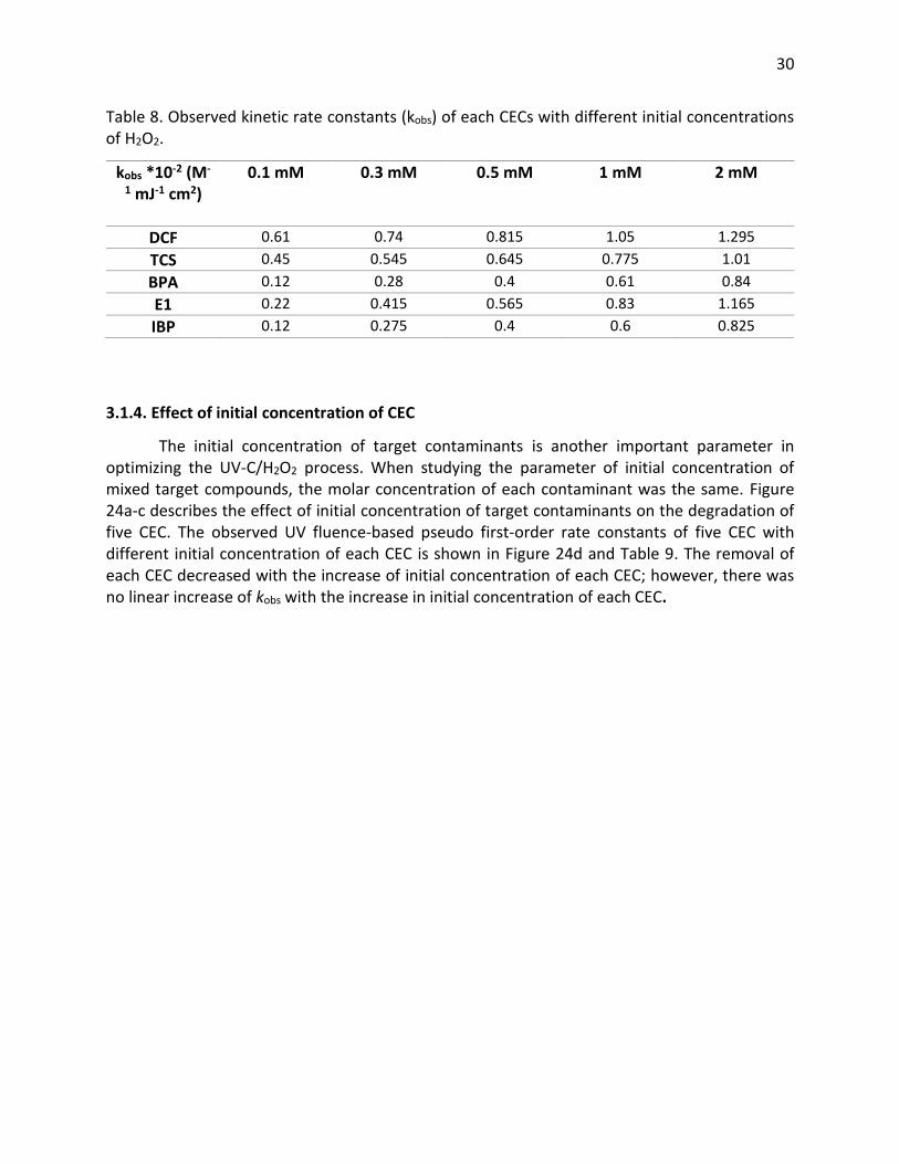
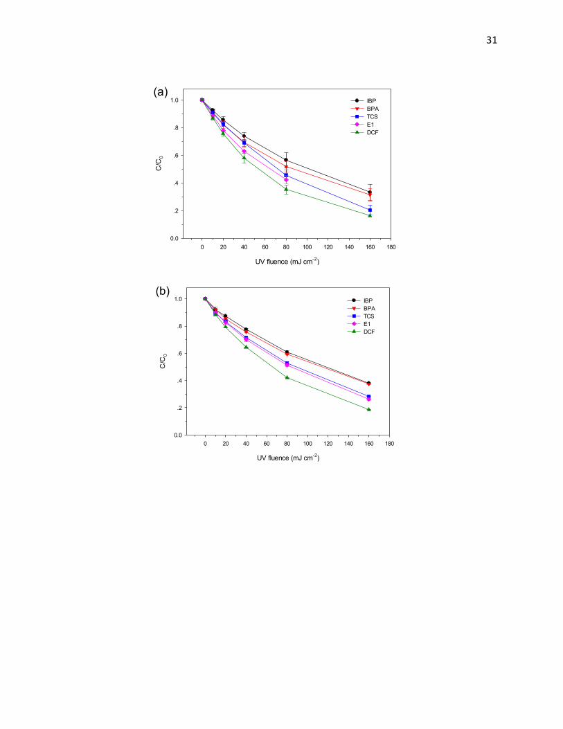
3.1.4. Effect of initial concentration of CEC

The initial concentration of target contaminants is another important parameter in optimizing the UV-C/H2O2 process. When studying the parameter of initial concentration of mixed target compounds, the molar concentration of each contaminant was the same. Figure 24a-c describes the effect of initial concentration of target contaminants on the degradation of five CEC. The observed UV fluence-based pseudo first-order rate constants of five CEC with different initial concentration of each CEC is shown in Figure 24d and Table 9. The removal of each CEC decreased with the increase of initial concentration of each CEC; however, there was no linear increase of kobs with the increase in initial concentration of each CEC.

31


0 20 40 60 80 100 120 140 160 180

C/C

0

0.0

.2

.4

.6

.8

1.0 IBPBPATCSE1DCF

(a)


0 20 40 60 80 100 120 140 160 180

C/C

0

0.0

.2

.4

.6

.8


(b)

32


0 20 40 60 80 100 120 140 160 180

C/C

0

0.0

.2

.4

.6

.8

1.0 IBPBPAE1TCSDCF

(c)

DCF TCS BPA E1 IBP

k obs

(x 1

0-2 c

m2 m

J-1)

0.0

.2

.4

.6

.8

1.0

1.2

1.4

1.60.5 uM 1 uM 2 uM

(d)

Figure 24. Degradation of the mixture of five CEC by UV-C/H2O2 with initial concentration of each CEC as 0.5 µM (a), 1 µM (b), and 2 µM (c); the observed kinetic rate constants of each CEC with different initial concentrations of each CEC (d). Experimental conditions: [DCF]0 = [TCS]0 = [BPA]0

= [E1]0 = [IBP]0, [H2O2]0 = 1 mM, 10 mM phosphate buffer (pH = 7.4).

33

Table 9. Observed kinetic rate constants (kobs) of each CECs with different initial concentrations of each CEC.

kobs *10-2 (M-1 mJ-1 cm2)

0.5 µM 1 µM 2 µM

DCF 1.29 1.05 0.83 TCS 1.005 0.775 0.64 BPA 0.725 0.61 0.415 E1 1.075 0.83 0.55 IBP 0.7 0.6 0.39

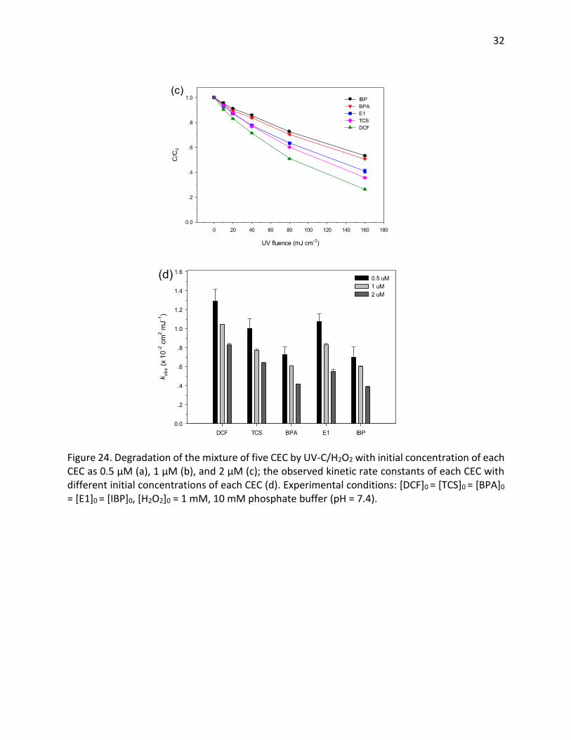
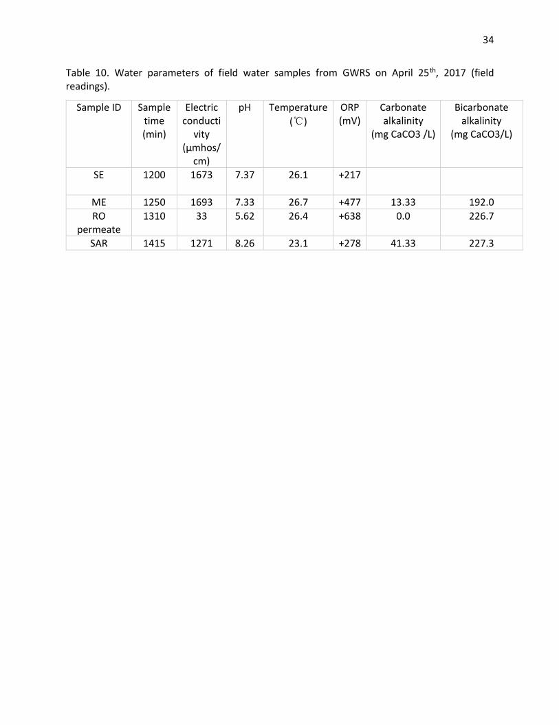
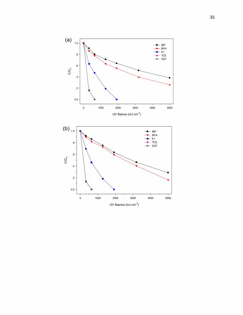
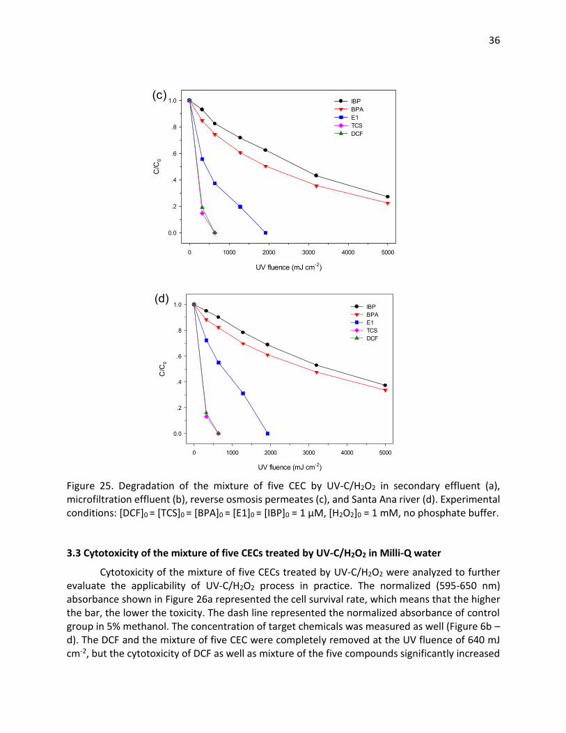
3.2 Degradation of the mixture of five CEC by UV-C/H2O2 in field water samples

Field water samples were used to evaluate the applicability of UV-C/H2O2 process in the degradation of mixed contaminants. Field water samples were obtained from Orange County Ground Water Replenishment System (GWRS) on April 25th, 2017, including secondary effluent (SE; the influent to the GWRS facility), microfiltration effluent (ME), reverse osmosis (RO) permeate, and Santa Ana River (SAR). Table 10 shows the parameters of these field water samples. Figure 25a-d describes the degradation of five CEC in secondary effluent (25a), microfiltration effluent (25b), reverse osmosis permeates (25c), and Santa Ana river (25d). Only DCF and TCS could be effectively degraded in these four field water samples, which also could be degraded by UV alone. E1 could be decomposed after the UV fluence of 1920 mJ cm-2. BPA and IBP at initial concentration of 1 µM could not be removed from these four field water samples even after the UV fluence of 5000 mJ cm-2. The efficiency of UV-C/H2O2 to remove these five CECs in field water samples from GWRS decreased dramatically, which might be ascribed to the presence of chloramine (Eqs. (6)). In the treatment process in GWRS, NaClO was added into the wastewater after secondary treatment, and before RO permeate. NaClO would react with present NH4+ to form chloramine.

NH2Cl + 3H2O2 → Cl− + NO3− + 2H+ + 3H2O (6)

34

Table 10. Water parameters of field water samples from GWRS on April 25th, 2017 (field readings).

Sample ID Sample time (min)

Electric conducti

vity (µmhos/

cm)

pH Temperature (℃)

ORP (mV)

Carbonate alkalinity

(mg CaCO3 /L)

Bicarbonate alkalinity

(mg CaCO3/L)

SE 1200 1673 7.37

26.1 +217

ME 1250 1693 7.33 26.7 +477 13.33 192.0 RO

permeate 1310 33 5.62 26.4 +638 0.0 226.7

SAR 1415 1271 8.26 23.1 +278 41.33 227.3

35


0 1000 2000 3000 4000 5000

C/C

0

0.0

.2

.4

.6

.8

1.0IBPBPAE1TCSDCF

(a)


0 1000 2000 3000 4000 5000

C/C

0

0.0

.2

.4

.6

.8

1.0 IBPBPAE1TCSDCF

(b)

36


0 1000 2000 3000 4000 5000

C/C

0

0.0

.2

.4

.6

.8

1.0 IBPBPAE1TCSDCF

(c)


0 1000 2000 3000 4000 5000

C/C

0

0.0

.2

.4

.6

.8

1.0 IBPBPAE1TCSDCF

(d)

Figure 25. Degradation of the mixture of five CEC by UV-C/H2O2 in secondary effluent (a), microfiltration effluent (b), reverse osmosis permeates (c), and Santa Ana river (d). Experimental conditions: [DCF]0 = [TCS]0 = [BPA]0 = [E1]0 = [IBP]0 = 1 µM, [H2O2]0 = 1 mM, no phosphate buffer.

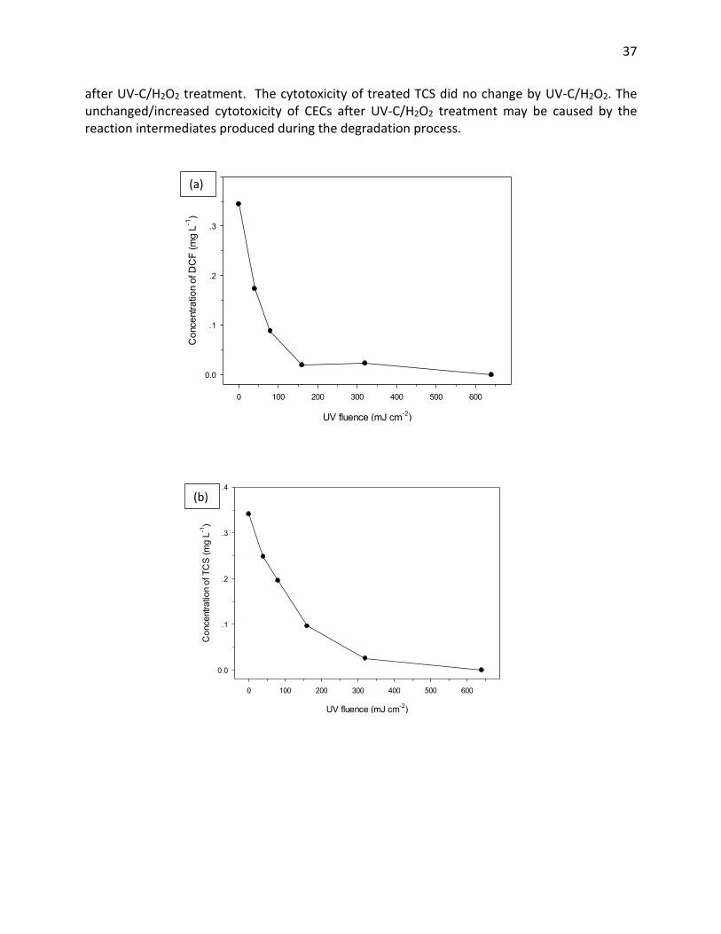
3.3 Cytotoxicity of the mixture of five CECs treated by UV-C/H2O2 in Milli-Q water

Cytotoxicity of the mixture of five CECs treated by UV-C/H2O2 were analyzed to further evaluate the applicability of UV-C/H2O2 process in practice. The normalized (595-650 nm) absorbance shown in Figure 26a represented the cell survival rate, which means that the higher the bar, the lower the toxicity. The dash line represented the normalized absorbance of control group in 5% methanol. The concentration of target chemicals was measured as well (Figure 6b –d). The DCF and the mixture of five CEC were completely removed at the UV fluence of 640 mJ cm-2, but the cytotoxicity of DCF as well as mixture of the five compounds significantly increased

37

after UV-C/H2O2 treatment. The cytotoxicity of treated TCS did no change by UV-C/H2O2. The unchanged/increased cytotoxicity of CECs after UV-C/H2O2 treatment may be caused by the reaction intermediates produced during the degradation process.


0 100 200 300 400 500 600

Con

cent

ratio

n of

DC

F (m

g L-1

)

0.0

.1

.2

.3

.4(b)


0 100 200 300 400 500 600

Con

cent

ratio

n of

TC

S (m

g L-1

)

0.0

.1

.2

.3

.4(c)

(a)

(b)

38


0 100 200 300 400 500 600

Con

cent

ratio

n (m

g L-1

)

0.0

.1

.2

.3DCFTCSBPAE1IBP

(d)

Figure 26. Cytotoxicity analysis of treated DCF, TCS, and five mixed CEC by UV-C/H2O2 using MTT assay (toxicology figure 43); corresponding concentration of treated DCF (a), TCS (b), and five mixed CEC (c) by UV-C/H2O2. The higher the bar, the lower the toxicity; bar below the dashed line indicates the exposure caused >20% mortality. Data bars represent the mean rSEM (n=3). Experimental conditions: [DCF]0 = [TCS]0 = [BPA]0 = [E1]0 = [IBP]0 = 1 µM, [H2O2]0 = 1 mM, 10 mM phosphate buffer (pH = 7.4).

(c)

39

4. Photocatalytic degradation of individual and mixed contaminants in clean water and water samples from GWRS water purification system in Orange County, CA

4.1. Photocatalyst synthesis

Nitrogen- and boron- co-doped TiO2 nanoparticles (NB-TiO2) were hydrothermally synthesized at three different (N+B):Ti atomic percentages (i.e., 0.06:1, 0.12:1, and 0.18:1). Borane (tert-butylamine complex) was used as a substrate for N and B. The three catalysts are given the following short names based on the dopant atomic percentage 6%-NB-TiO2, 12%-NB-TiO2 and 18%-NB-TiO2.

To synthesize the catalysts, a 7.0 mL of titanium (IV) butoxide was added dropwise to a 100-mL size Teflon hydrothermal vessel containing a mixture of 50 mL ethyl alcohol and 2.0 mL glacial acetic acid. A certain amount of borane pellets (i.e., corresponding to the desired doping ratio) was dissolved in 10.0 mL ethyl alcohol and then was added to the previous mixture, followed by a dropwise addition of 2.0 mL Milli-Q H2O under vigorous stirring for 20 min at room temperature, with the vessel’s cap on. The mixture was then placed in a furnace at 180 ºC for 20 hrs under a temperature ramp rate of 150 ºC/hr. The supernatant solution was then separated from the pale-yellow precipitate by decantation. The precipitate was dried at 80 ºC for 6 hrs. Afterwards, the dried precipitate was grinded using a mortar and transferred to a 50-mL clean porcelain crucible to be furtherly calcined at 350 ºC for 10 hrs at 150 ºC/hr ramp rate.

4.2. Photocatalyst characterization

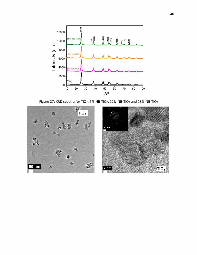
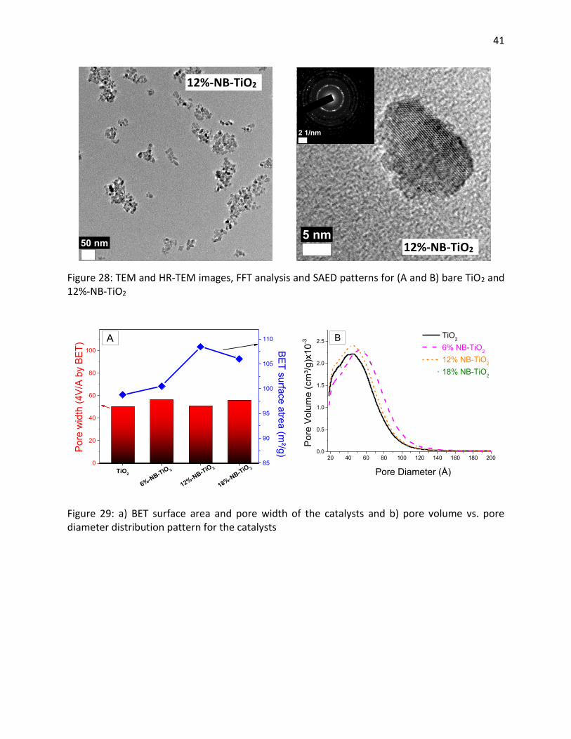
Different spectroscopic and texture analysis techniques were utilized to elucidate the structure of the prepared catalysts including X-ray diffraction (XRD), Scanning Electron Microscopy (SEM), Energy Dispersive X-ray spectroscopy (EDX), Transmittance Electron Microscopy (TEM), High resolution-TEM (HR-TEM) and Brunauer-Emmett-Teller (BET) porosity analysis.

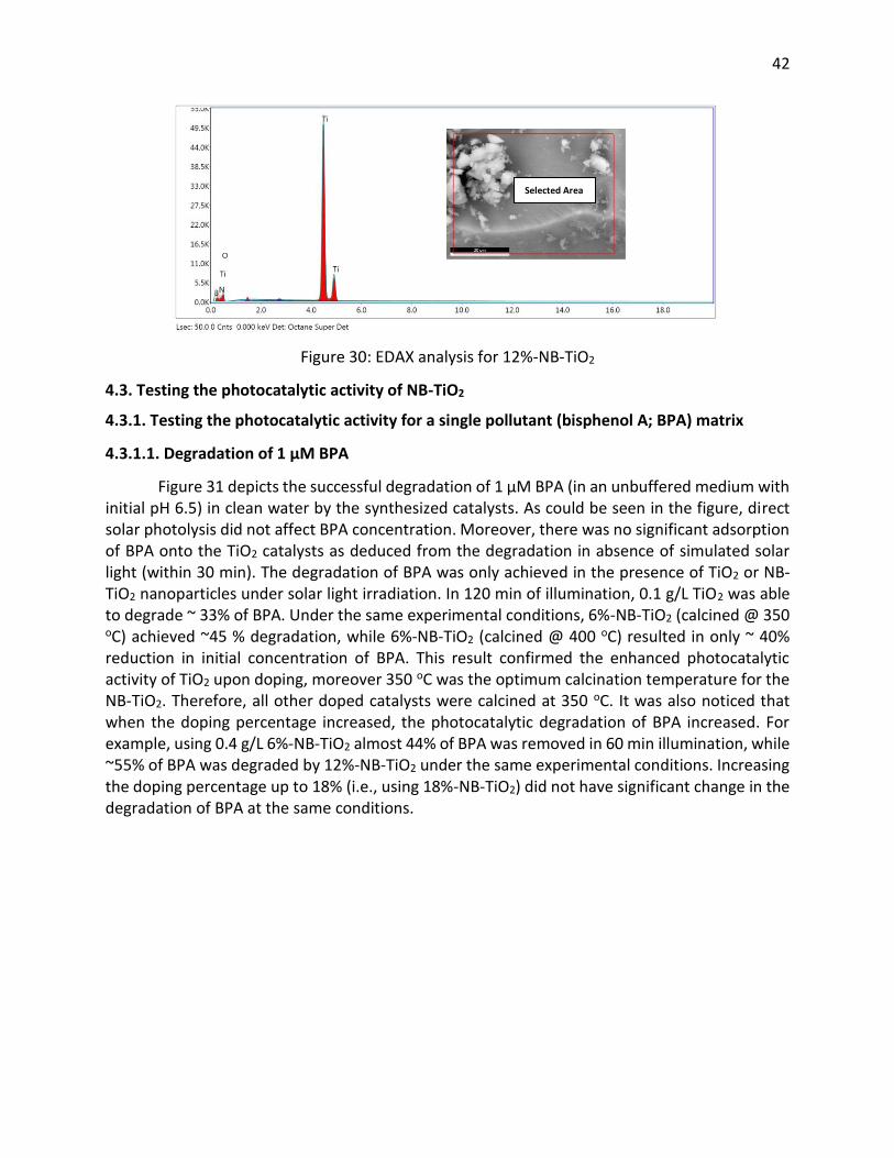
Figure 27 depicts the XRD results of photocatalysts. All spectra analysis confirmed the existence of TiO2 and NB-TiO2 in monocrystalline, anatase phase. The particle size calculated from XRD using Scherrer’s equation was ~9 nm for all catalysts. TEM images (Figure 28) confirmed the same average particle size. Average pore width and volume as well as BET surface areas of the prepared nanoparticles are depicted in figure 29A and B. Among all the prepared catalysts, 12%-NB-TiO2 had the highest surface area (108.5 m2/g) and pore volume (0.0024 cm3/g). Pore diameter and width did not change to much in all catalysts. EDX analysis (Figure 30) showed the presence of N and B in the TiO2 crystal lattice, confirming the doping process by the current method was successful.

40

10 20 30 40 50 60 70 80 900

2000

4000

6000

8000

10000

12000

(215

)(200

)

(220

)(1

16)

(204

)

(211

)(1

05)

(004

)(1

03)

18% NB-TiO2

12% NB-TiO2

6% NB-TiO2

TiO2

Inte

nsity

(a. u

.)

2T�

(101

)

Figure 27: XRD spectra for TiO2, 6%-NB-TiO2, 12%-NB-TiO2 and 18%-NB-TiO2

50 nm

2 nm

2 1/nm

TiO2

TiO2

41

50 nm

5 nm

2 1/nm

Figure 28: TEM and HR-TEM images, FFT analysis and SAED patterns for (A and B) bare TiO2 and 12%-NB-TiO2

85

90

95

100

105

110

0

20

40

60

80

100

Pore

wid

th (4

V/A

by B

ET) A

18%-NB-TiO 2

12%-NB-TiO 2

6%-NB-TiO 2

BET surface atrea (m²/g)

TiO2

20 40 60 80 100 120 140 160 180 2000.0

0.5

1.0

1.5

2.0

2.5 B TiO2

6% NB-TiO2

12% NB-TiO2

18% NB-TiO2

Por

e V

olum

e (c

m³/g

)x10

-3

Pore Diameter (Å)

Figure 29: a) BET surface area and pore width of the catalysts and b) pore volume vs. pore diameter distribution pattern for the catalysts

12%-NB-TiO2

12%-NB-TiO2

42

Figure 30: EDAX analysis for 12%-NB-TiO2

4.3. Testing the photocatalytic activity of NB-TiO2

4.3.1. Testing the photocatalytic activity for a single pollutant (bisphenol A; BPA) matrix

4.3.1.1. Degradation of 1 µM BPA

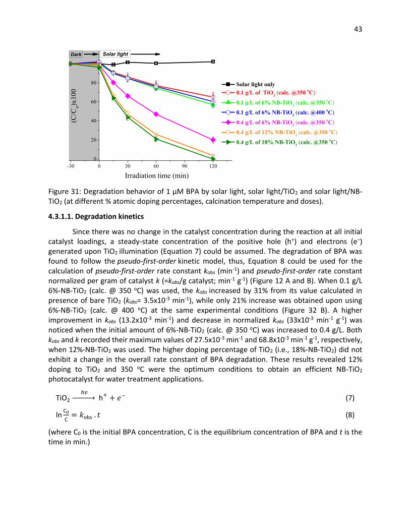
Figure 31 depicts the successful degradation of 1 µM BPA (in an unbuffered medium with initial pH 6.5) in clean water by the synthesized catalysts. As could be seen in the figure, direct solar photolysis did not affect BPA concentration. Moreover, there was no significant adsorption of BPA onto the TiO2 catalysts as deduced from the degradation in absence of simulated solar light (within 30 min). The degradation of BPA was only achieved in the presence of TiO2 or NB-TiO2 nanoparticles under solar light irradiation. In 120 min of illumination, 0.1 g/L TiO2 was able to degrade ~ 33% of BPA. Under the same experimental conditions, 6%-NB-TiO2 (calcined @ 350 oC) achieved ~45 % degradation, while 6%-NB-TiO2 (calcined @ 400 oC) resulted in only ~ 40% reduction in initial concentration of BPA. This result confirmed the enhanced photocatalytic activity of TiO2 upon doping, moreover 350 oC was the optimum calcination temperature for the NB-TiO2. Therefore, all other doped catalysts were calcined at 350 oC. It was also noticed that when the doping percentage increased, the photocatalytic degradation of BPA increased. For example, using 0.4 g/L 6%-NB-TiO2 almost 44% of BPA was removed in 60 min illumination, while ~55% of BPA was degraded by 12%-NB-TiO2 under the same experimental conditions. Increasing the doping percentage up to 18% (i.e., using 18%-NB-TiO2) did not have significant change in the degradation of BPA at the same conditions.

Selected Area

43

-30 0 30 60 90 1200

20

40

60

80

100

Solar light

(C/C

o)x1

00

Irradiation time (min)

Solar light only 0.1 g/L of TiO2 (calc. @350 oC)

0.1 g/L of 6% NB-TiO2 (calc. @350 oC)





Dark

Figure 31: Degradation behavior of 1 µM BPA by solar light, solar light/TiO2 and solar light/NB-TiO2 (at different % atomic doping percentages, calcination temperature and doses).

4.3.1.1. Degradation kinetics

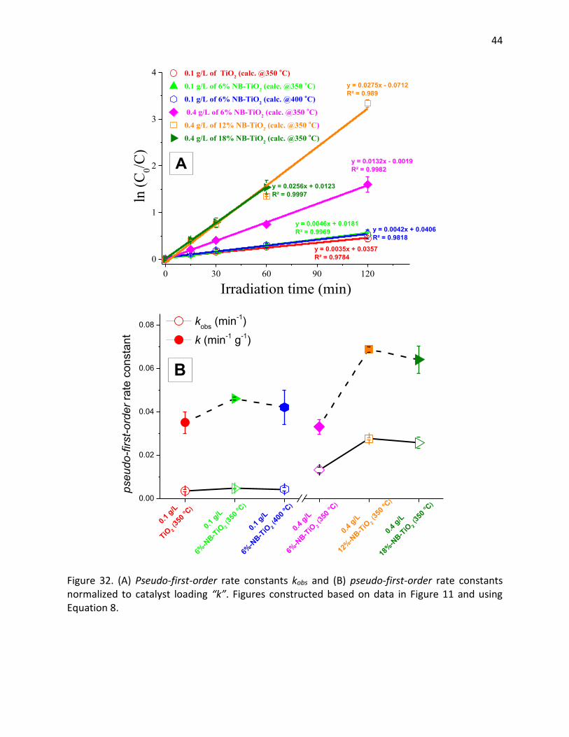
Since there was no change in the catalyst concentration during the reaction at all initial catalyst loadings, a steady-state concentration of the positive hole (h+) and electrons (e–) generated upon TiO2 illumination (Equation 7) could be assumed. The degradation of BPA was found to follow the pseudo-first-order kinetic model, thus, Equation 8 could be used for the calculation of pseudo-first-order rate constant kobs (min-1) and pseudo-first-order rate constant normalized per gram of catalyst k (=kobs/g catalyst; min-1 g-1) (Figure 12 A and B). When 0.1 g/L 6%-NB-TiO2 (calc. @ 350 oC) was used, the kobs increased by 31% from its value calculated in presence of bare TiO2 (kobs= 3.5x10-3 min-1), while only 21% increase was obtained upon using 6%-NB-TiO2 (calc. @ 400 oC) at the same experimental conditions (Figure 32 B). A higher improvement in kobs (13.2x10-3 min-1) and decrease in normalized kobs (33x10-3 min-1 g-1) was noticed when the initial amount of 6%-NB-TiO2 (calc. @ 350 oC) was increased to 0.4 g/L. Both kobs and k recorded their maximum values of 27.5x10-3 min-1 and 68.8x10-3 min-1 g-1, respectively, when 12%-NB-TiO2 was used. The higher doping percentage of TiO2 (i.e., 18%-NB-TiO2) did not exhibit a change in the overall rate constant of BPA degradation. These results revealed 12% doping to TiO2 and 350 oC were the optimum conditions to obtain an efficient NB-TiO2 photocatalyst for water treatment applications.

TiO2 ℎ𝑣 → h+ + 𝑒− (7)

ln C0

C= 𝑘obs . 𝑡 (8)

(where C0 is the initial BPA concentration, C is the equilibrium concentration of BPA and t is the time in min.)

44

0 30 60 90 1200

1

2

3

4

A

y = 0.0046x + 0.0181R² = 0.9969 y = 0.0042x + 0.0406

R² = 0.9818

y = 0.0035x + 0.0357R² = 0.9784

y = 0.0132x - 0.0019R² = 0.9982

y = 0.0275x - 0.0712R² = 0.989

y = 0.0256x + 0.0123R² = 0.9997

0.1 g/L of TiO2 (calc. @350 oC)





0.4 g/L of 18% NB-TiO2 (calc. @350 oC)ln

(C0/C

)


0.00

0.02

0.04

0.06

0.08

0.4

g/L

18%-N

B-TiO 2 (3

50 o C)

0.4 g/L

12%-N

B-TiO 2 (3

50 o C)

0.4

g/L

6%-N

B-TiO 2 (3

50 o C)

0.1

g/L

6%-N

B-TiO 2 (4

00 o C)

0.1

g/L

6%-N

B-TiO 2 (3

50 o C)

0.

1 g/L

TiO 2 (3

50 o C)

pseudo-first-order

rate

con

stan

t

kobs (min-1) k (min-1 g-1)

B

Figure 32. (A) Pseudo-first-order rate constants kobs and (B) pseudo-first-order rate constants normalized to catalyst loading “k”. Figures constructed based on data in Figure 11 and using Equation 8.

45

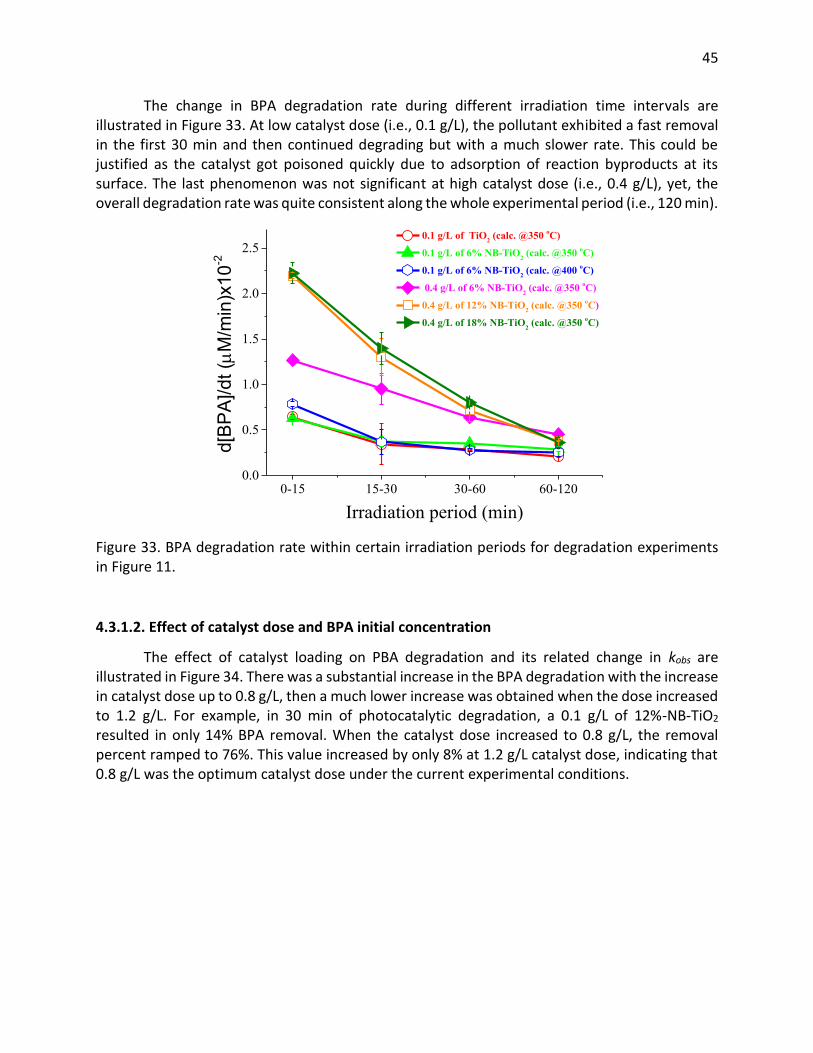
The change in BPA degradation rate during different irradiation time intervals are illustrated in Figure 33. At low catalyst dose (i.e., 0.1 g/L), the pollutant exhibited a fast removal in the first 30 min and then continued degrading but with a much slower rate. This could be justified as the catalyst got poisoned quickly due to adsorption of reaction byproducts at its surface. The last phenomenon was not significant at high catalyst dose (i.e., 0.4 g/L), yet, the overall degradation rate was quite consistent along the whole experimental period (i.e., 120 min).

0-15 15-30 30-60 60-1200.0

0.5

1.0

1.5

2.0

2.5 0.1 g/L of TiO2 (calc. @350 oC)






d[

BPA]

/dt (PM

/min

)x10

-2

Irradiation period (min)

Figure 33. BPA degradation rate within certain irradiation periods for degradation experiments in Figure 11.

4.3.1.2. Effect of catalyst dose and BPA initial concentration

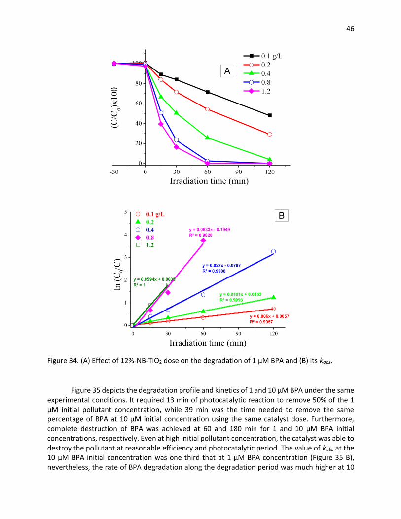
The effect of catalyst loading on PBA degradation and its related change in kobs are illustrated in Figure 34. There was a substantial increase in the BPA degradation with the increase in catalyst dose up to 0.8 g/L, then a much lower increase was obtained when the dose increased to 1.2 g/L. For example, in 30 min of photocatalytic degradation, a 0.1 g/L of 12%-NB-TiO2 resulted in only 14% BPA removal. When the catalyst dose increased to 0.8 g/L, the removal percent ramped to 76%. This value increased by only 8% at 1.2 g/L catalyst dose, indicating that 0.8 g/L was the optimum catalyst dose under the current experimental conditions.

46

-30 0 30 60 90 1200

20

40

60

80

100 A

(C/C

o)x10

0


0.1 g/L 0.2 0.4 0.8 1.2

0 30 60 90 1200

1

2

3

4

5

y = 0.0594x + 0.0035R² = 1

y = 0.0633x - 0.1949R² = 0.9828

y = 0.027x - 0.0797R² = 0.9908

y = 0.0101x + 0.0153R² = 0.9993

y = 0.006x + 0.0057R² = 0.9957

0.1 g/L 0.2 0.4 0.8 1.2

ln (C

0/C)


B

Figure 34. (A) Effect of 12%-NB-TiO2 dose on the degradation of 1 µM BPA and (B) its kobs.

Figure 35 depicts the degradation profile and kinetics of 1 and 10 µM BPA under the same experimental conditions. It required 13 min of photocatalytic reaction to remove 50% of the 1 µM initial pollutant concentration, while 39 min was the time needed to remove the same percentage of BPA at 10 µM initial concentration using the same catalyst dose. Furthermore, complete destruction of BPA was achieved at 60 and 180 min for 1 and 10 µM BPA initial concentrations, respectively. Even at high initial pollutant concentration, the catalyst was able to destroy the pollutant at reasonable efficiency and photocatalytic period. The value of kobs at the 10 µM BPA initial concentration was one third that at 1 µM BPA concentration (Figure 35 B), nevertheless, the rate of BPA degradation along the degradation period was much higher at 10

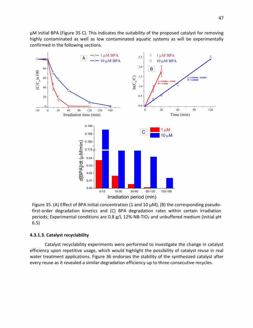
47

µM initial BPA (Figure 35 C). This indicates the suitability of the proposed catalyst for removing highly contaminated as well as low contaminated aquatic systems as will be experimentally confirmed in the following sections.

-30 0 30 60 90 120 150 1800

20

40

60

80

100

(C/C

o)x1

00


1 PM BPA 10 PM BPA A

0 30 60 90 1200.0

0.5

1.0

1.5

2.0

2.5

B

y = 0.02028x - 0.02847R² = 0.99988

y = 0.0593x - 0.0078R² = 0.9995

1 PM BPA 10 PM BPA

ln(C

0/C)

Time (min)

0-15 15-30 30-60 60-120 120-1800.00

0.01

0.02

0.03

0.04

0.175

0.180

0.185

0.190

C

d[BP

A]/d

t (PM

/min

)

Irradiation period (min)

1 PM 10 PM

Figure 35. (A) Effect of BPA initial concentration (1 and 10 µM), (B) the corresponding pseudo-first-order degradation kinetics and (C) BPA degradation rates within certain irradiation periods; Experimental conditions are 0.8 g/L 12%-NB-TiO2 and unbuffered medium (initial pH 6.5)

4.3.1.3. Catalyst recyclability

Catalyst recyclability experiments were performed to investigate the change in catalyst efficiency upon repetitive usage, which would highlight the possibility of catalyst reuse in real water treatment applications. Figure 36 endorses the stability of the synthesized catalyst after every reuse as it revealed a similar degradation efficiency up to three consecutive recycles.

48

0 60 120

0

20

40

60

80

100

0 60 120 0 60 120


1st 2nd

([BP

A]/[

BP

A] 0)

x100

3rd

Figure 36. Catalyst recycles. Experimental conditions: 0.8 g/L 12%-NB-TiO2, 1 µM BPA and unbuffered medium (initial pH 6.5)

4.3.1.4. Reaction byproducts and pathways

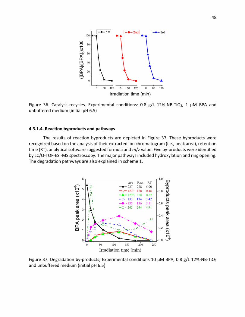
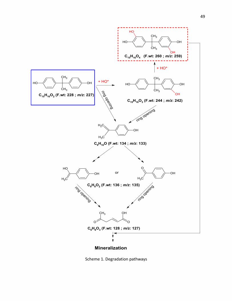
The results of reaction byproducts are depicted in Figure 37. These byproducts were recognized based on the analysis of their extracted ion chromatogram (i.e., peak area), retention time (RT), analytical software suggested formula and m/z value. Five by-products were identified by LC/Q-TOF-ESI-MS spectroscopy. The major pathways included hydroxylation and ring opening. The degradation pathways are also explained in scheme 1.

0

1

2

3

4

5

6

0 50 100 150 200 2500.0

0.2

0.4

0.6

0.8

1.0

BP

A p

eak

area

(x10

6 ) 227 228 5.90

Byproducts peak area (x10

6)


m/z F.wt RT

127i 128 0.46 127ii 128 0.62 133 134 3.42 135 136 3.51 242 244 4.91

Figure 37. Degradation by-products; Experimental conditions 10 µM BPA, 0.8 g/L 12%-NB-TiO2 and unbuffered medium (initial pH 6.5)

49

CH3

CH3

OHOH

C15H16O2 (F.wt: 228 ; m/z: 227)CH3

CH3

OHOH

OH

C15H16O3 (F.wt: 244 ; m/z: 242)

CH3

CH3

OHOH

OH

OH

C15H16O4 (F.wt: 260 ; m/z: 259)

CH3

CH2

OH

C9H10O (F.wt: 134 ; m/z: 133)

OH

OH

CH2

C8H8O2 (F.wt: 136 ; m/z: 135)

OH

O

CH3

O

CH3

O

OH

C6H8O3 (F.wt: 128 ; m/z: 127)

or

+ HO*

+ HO*

ring openingring opening

ring opening ring o

penin

g

Mineralization

Scheme 1. Degradation pathways

50

4.3.2. Degradation of a mixture of pollutants (BPA, E1, DCF, IBP and TCS) using 0.8 g/L of 12%-NB-TiO2 catalyst.

4.3.2.1. Effect of pH on the degradation of 1 µM mixture of BPA, E1, DCF, IBP and TCS in Milli-Q water

In TiO2 photocatalysis, reactive radical species are released via reactions represented in Equations (9) and (10). These species are the key factor in the degradation of pollutants. They attack organic substrates and lead to their degradation. The equilibrium release of these radical is pH dependent. For instance, acidic medium suppresses the HO● species generated via reaction of water molecules with the catalyst H+ (Equation 10), hence, the photocatalytic efficiency of TiO2 decreases. Moreover, at high basic medium, quenching effect exists between the oxygen radical species and hydroxyl ions.

𝑒− + O2 → O2

●− (9)

H+ + H2O → HO● + H+ (10)

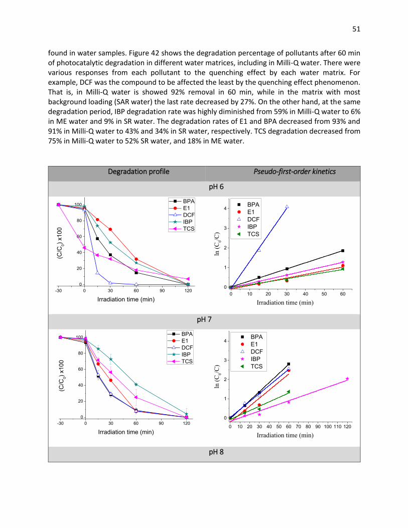
The impact of pH (i.e., 6, 7 and 8) on the degradation of the five pollutants is depicted in Figure 38. The initial pH was adjusted using 0.1 N HCl and NaOH. To be noted, the value of pH after 120 min of photocatalytic reaction did not undergo any notable change from its initial value in all systems (i.e., ~0.2 – 0.3 decrease). Experiments conducted under dark conditions revealed only TCS 55% removal at pH 6 due to its adsorption onto the catalyst surface. This phenomenon was previously revealed to occur as a result of the electrostatic interaction between TCS and TiO2 in acidic medium. Under solar light, the pollutants showed different degradation trends under different pH conditions. Moreover, complete removal of all pollutants was obtained after 120 min treatment in all systems, except for TCS at pH 6 and IBP at pH 8, they showed 90 and 80% degradation at the same degradation period. Based on kobs values at different pH values (Figure 39), pH 7 exhibited the optimum removal of all pollutants, except for DCF which displayed exceptionally high removal at pH 6. Therefore, considering the effect of pH on both TiO2 adsorption and photocatalysis, further degradation experiments in field water matrices were conducted at pH 7.

4.3.2.2. Degradation of a mixture of BPA, E1, DCF, IBP and TCS in field water matrices

The photocatalytic potency of 12%-NB-TiO2 for the degradation of a mixture of five pollutants (1 µM each) was examined in different field water matrices (Figure 40). The tested waters were collected from GWRS water purification system in Orange County, at different treatment stages including SE and ME. In addition, experiments were also performed in raw water from SAR to compare the results. The degradation of all five pollutants was found to fit a pseudo-first-order model as shown in Figure 40, with the values of kobs depicted in Figure 41.

Initial water parameters such as electrical conductivity (EC), pH, oxidation-reduction potential (ORP) and carbonate and bicarbonate alkalinities are depicted in Table 11. Generally, the degradation of pollutants in real water matrices was less than in Milli-Q water. This could be due to the quenching effect by the real water constituents such as carbonates and bicarbonates (represented by alkalinity measure in Table 11), as well as the organic matter that is originally

51

found in water samples. Figure 42 shows the degradation percentage of pollutants after 60 min of photocatalytic degradation in different water matrices, including in Milli-Q water. There were various responses from each pollutant to the quenching effect by each water matrix. For example, DCF was the compound to be affected the least by the quenching effect phenomenon. That is, in Milli-Q water is showed 92% removal in 60 min, while in the matrix with most background loading (SAR water) the last rate decreased by 27%. On the other hand, at the same degradation period, IBP degradation rate was highly diminished from 59% in Milli-Q water to 6% in ME water and 9% in SR water. The degradation rates of E1 and BPA decreased from 93% and 91% in Milli-Q water to 43% and 34% in SR water, respectively. TCS degradation decreased from 75% in Milli-Q water to 52% SR water, and 18% in ME water.

Degradation profile Pseudo-first-order kinetics

pH 6

-30 0 30 60 90 1200

20

40

60

80

100

(C/C

0) x10

0


BPA E1 DCF IBP TCS

0 10 20 30 40 50 60

0

1

2

3

4


ln (C

0/C)

BPA E1 DCF IBP TCS

pH 7

-30 0 30 60 90 1200

20

40

60

80

100

(C/C

0) x

100


BPA E1 DCF IBP TCS

0 10 20 30 40 50 60 70 80 90 100 110 120

0

1

2

3

4


ln (C

0/C)

BPA E1 DCF IBP TCS

pH 8

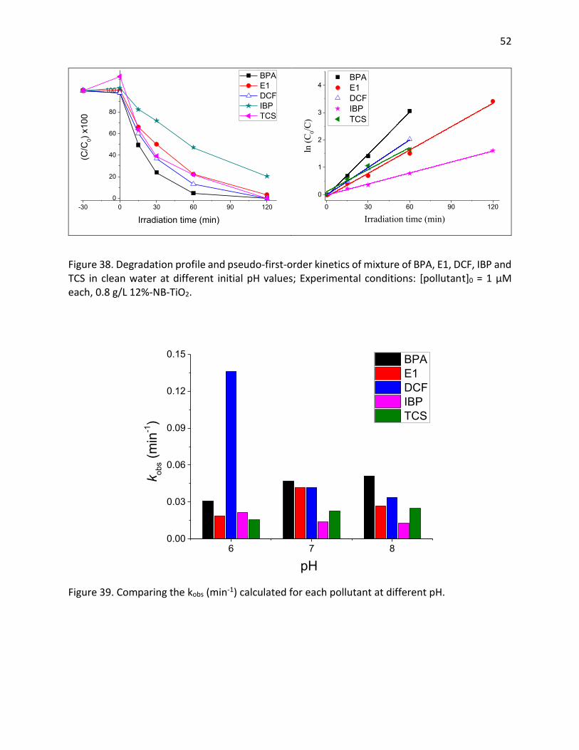
52

-30 0 30 60 90 1200

20

40

60

80

100(C

/C0)

x10

0


BPA E1 DCF IBP TCS

0 30 60 90 120

0

1

2

3

4


ln (C

0/C)

BPA E1 DCF IBP TCS

Figure 38. Degradation profile and pseudo-first-order kinetics of mixture of BPA, E1, DCF, IBP and TCS in clean water at different initial pH values; Experimental conditions: [pollutant]0 = 1 µM each, 0.8 g/L 12%-NB-TiO2.

6 7 80.00

0.03

0.06

0.09

0.12

0.15

k obs

(min

-1)

pH

BPA E1 DCF IBP TCS

Figure 39. Comparing the kobs (min-1) calculated for each pollutant at different pH.

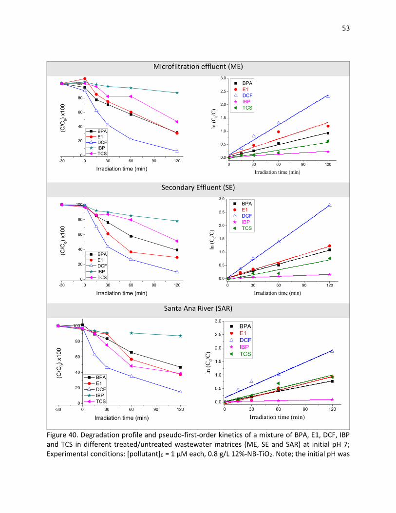
53

Microfiltration effluent (ME)

-30 0 30 60 90 1200

20

40

60

80

100

(C/C

0) x10

0


BPA E1 DCF IBP TCS

0 30 60 90 120

0.0

0.5

1.0

1.5

2.0

2.5

3.0


ln (C

0/C)

BPA E1 DCF IBP TCS

Secondary Effluent (SE)

-30 0 30 60 90 1200

20

40

60

80

100

(C/C

0) x

100


BPA E1 DCF IBP TCS

0 30 60 90 120

0.0

0.5

1.0

1.5

2.0

2.5

3.0


ln (C

0/C)

BPA E1 DCF IBP TCS

Santa Ana River (SAR)

-30 0 30 60 90 1200

20

40

60

80

100

(C/C

0) x

100


BPA E1 DCF IBP TCS

0 30 60 90 120

0.0

0.5

1.0

1.5

2.0

2.5

3.0


ln (C

0/C)

BPA E1 DCF IBP TCS

Figure 40. Degradation profile and pseudo-first-order kinetics of a mixture of BPA, E1, DCF, IBP and TCS in different treated/untreated wastewater matrices (ME, SE and SAR) at initial pH 7; Experimental conditions: [pollutant]0 = 1 µM each, 0.8 g/L 12%-NB-TiO2. Note; the initial pH was

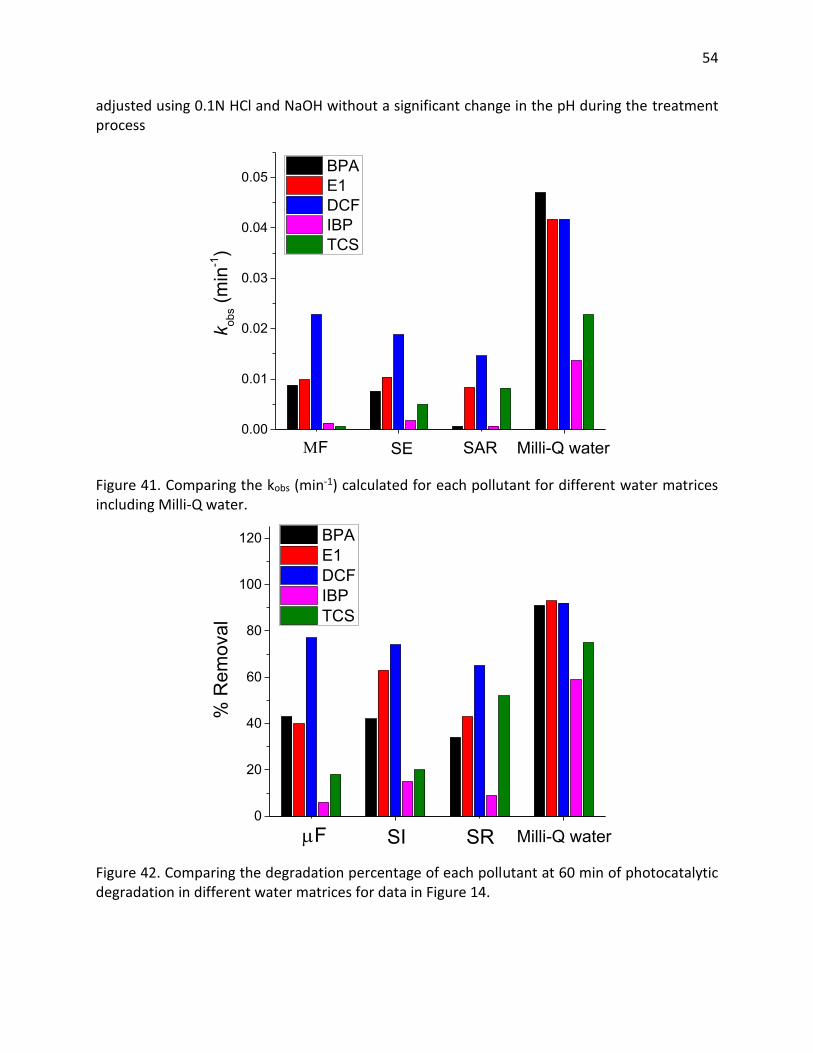
54

adjusted using 0.1N HCl and NaOH without a significant change in the pH during the treatment process

0.00

0.01

0.02

0.03

0.04

0.05

Milli-Q waterSARSE

k obs

(min

-1)

BPA E1 DCF IBP TCS

0F

Figure 41. Comparing the kobs (min-1) calculated for each pollutant for different water matrices including Milli-Q water.

0

20

40

60

80

100

120

SRSI

% R

emov

al

BPA E1 DCF IBP TCS

PF Milli-Q water

Figure 42. Comparing the degradation percentage of each pollutant at 60 min of photocatalytic degradation in different water matrices for data in Figure 14.

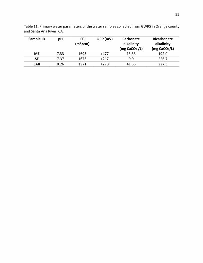
55

Table 11: Primary water parameters of the water samples collected from GWRS in Orange county and Santa Ana River, CA.

Sample ID pH EC (mS/cm)

ORP (mV) Carbonate alkalinity

(mg CaCO3 /L)

Bicarbonate alkalinity

(mg CaCO3/L) ME 7.33 1693 +477 13.33 192.0 SE 7.37 1673 +217 0.0 226.7

SAR 8.26 1271 +278 41.33 227.3

56

Toxicology Analysis 5.1. Assay Methods 5.1.1 MTT Cytotoxicity Assay Cell viability was determined by MTT assay(van de Loosdrecht et al., 1994). Cells were seeded at a concentration of 1x105 into a 96-well plate. After 24 h, cells were treated with SPE extracts and incubated for 16 h at 37qC. The media was then aspirated and replaced with serum-free media containing MTT (0.5 mg/mL) and incubated for 4 h at 37qC. The media was then discarded and replaced with 200 Pl of EtOH:DMSO (50:50) and shaken at moderate speed for 45 min. Absorbance was read at 595 nm and 650 nm using a Wallac Victor 2TM plate reader. Concentrations eliciting 80% survival or greater were deemed appropriate for receptor activity measurements.

5.1.2. Cell Assay Procedure

The estrogenic (ER) and aryl hydrocarbon receptor-like (AhR) activities of the extracts were assessed by using the established in vitro LUMI-CELL™ER (VM7Luc4E2) assay and AhR assay (GeneBLAzer CYP1A1-bla LS-180, Life Technologies, Carlsbad, CA). VM7Luc4E2 cells were graciously donated by Dr. Michael Denison (University of California-Davis).

VM7Luc4E2 cells were grown in RPMI 1640 with 5% fetal bovine serum. Four days prior to performing the assay, cells were transferred into flasks containing DMEM media (supplemented with 5% carbon stripped fetal calf serum and G418 sulfate solution). Cells were then plated in 96 well plates and incubated at 37qC for 24 hours prior to dosing. The media solution in each well was then removed and two hundred microliters of DMEM containing the desired chemical to be tested was added to each well and the plate was incubated for 16 hours. After lysing the cells (Promega lysis buffer), the luciferase activity was measured in a GLOMAX Multi Detection System (Promega), with automatic injection of 50 microliters of luciferase enzyme reagent (Promega) to each well. The relative light units (RLUs) measured were compared to that induced by the 17E-estradiol standard curve after subtraction of background activity.

GeneBLAzer AhR cells were purchased from Life Technologies. For the AhR assay, CYP1A1-bla LS-180 cells were cultured and used to measure AhR activity following the manufacturer’s protocols

(http://tools.lifetechnologies.com/content/sfs/manuals/geneblazer_cyp1a1blals0180_man.pdf)

5.2. Advanced Oxidation Treatments of GWRS Water 5.2.1. Cytotoxicity in AhR cell line Toxicology analysis of samples treated with different UV advanced oxidation processes by the University of Cincinnati.

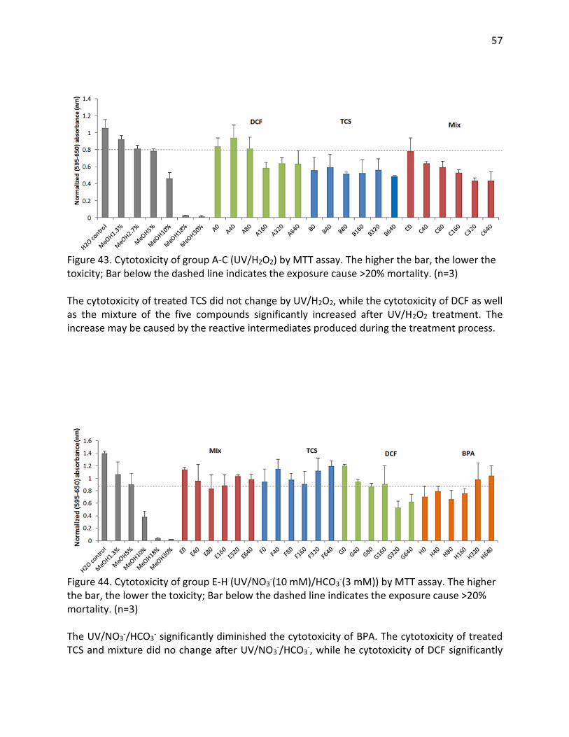
http://tools.lifetechnologies.com/content/sfs/manuals/geneblazer_cyp1a1blals0180_man.pdf

57

Figure 43. Cytotoxicity of group A-C (UV/H2O2) by MTT assay. The higher the bar, the lower the toxicity; Bar below the dashed line indicates the exposure cause >20% mortality. (n=3) The cytotoxicity of treated TCS did not change by UV/H2O2, while the cytotoxicity of DCF as well as the mixture of the five compounds significantly increased after UV/H2O2 treatment. The increase may be caused by the reactive intermediates produced during the treatment process.

Figure 44. Cytotoxicity of group E-H (UV/NO3-(10 mM)/HCO3-(3 mM)) by MTT assay. The higher the bar, the lower the toxicity; Bar below the dashed line indicates the exposure cause >20% mortality. (n=3) The UV/NO3-/HCO3- significantly diminished the cytotoxicity of BPA. The cytotoxicity of treated TCS and mixture did no change after UV/NO3-/HCO3-, while he cytotoxicity of DCF significantly

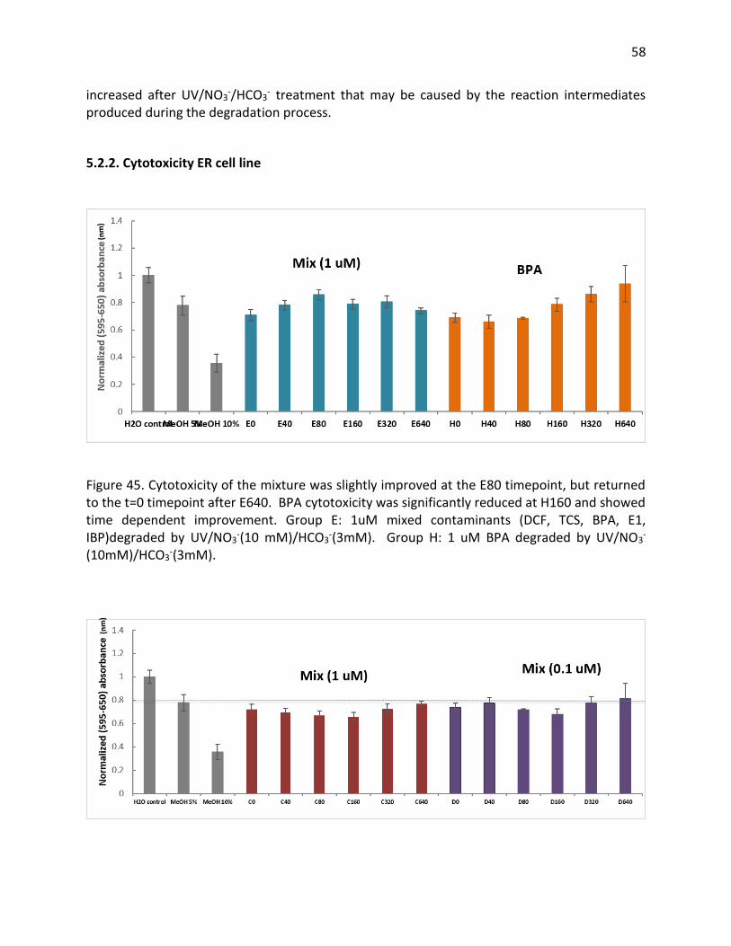
58

increased after UV/NO3-/HCO3- treatment that may be caused by the reaction intermediates produced during the degradation process. 5.2.2. Cytotoxicity ER cell line

Figure 45. Cytotoxicity of the mixture was slightly improved at the E80 timepoint, but returned to the t=0 timepoint after E640. BPA cytotoxicity was significantly reduced at H160 and showed time dependent improvement. Group E: 1uM mixed contaminants (DCF, TCS, BPA, E1, IBP)degraded by UV/NO3-(10 mM)/HCO3-(3mM). Group H: 1 uM BPA degraded by UV/NO3-

(10mM)/HCO3-(3mM).

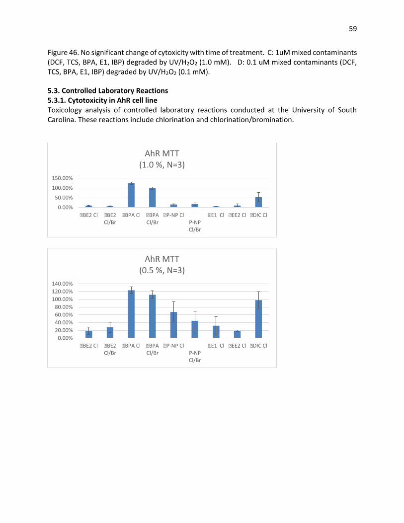
59

Figure 46. No significant change of cytoxicity with time of treatment. C: 1uM mixed contaminants (DCF, TCS, BPA, E1, IBP) degraded by UV/H2O2 (1.0 mM). D: 0.1 uM mixed contaminants (DCF, TCS, BPA, E1, IBP) degraded by UV/H2O2 (0.1 mM). 5.3. Controlled Laboratory Reactions 5.3.1. Cytotoxicity in AhR cell line Toxicology analysis of controlled laboratory reactions conducted at the University of South Carolina. These reactions include chlorination and chlorination/bromination.

0.00%

50.00%

100.00%

150.00%

�BE2 Cl �BE2Cl/Br

�BPA Cl �BPACl/Br

�P-NP ClP-NPCl/Br

�E1 Cl �EE2 Cl �DIC Cl

AhR MTT (1.0 %, N=3)

0.00%20.00%40.00%60.00%80.00%

100.00%120.00%140.00%



�P-NP ClP-NPCl/Br


AhR MTT (0.5 %, N=3)

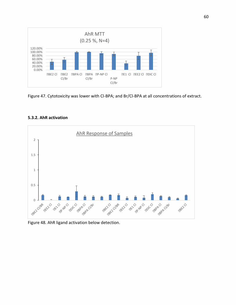
60

Figure 47. Cytotoxicity was lower with Cl-BPA; and Br/Cl-BPA at all concentrations of extract. 5.3.2. AhR activation

Figure 48. AhR ligand activation below detection.

0.00%20.00%40.00%60.00%80.00%

100.00%120.00%



�P-NP ClP-NPCl/Br


AhR MTT (0.25 %, N=4)

0

0.5

1

1.5

2

AhR Response of Samples

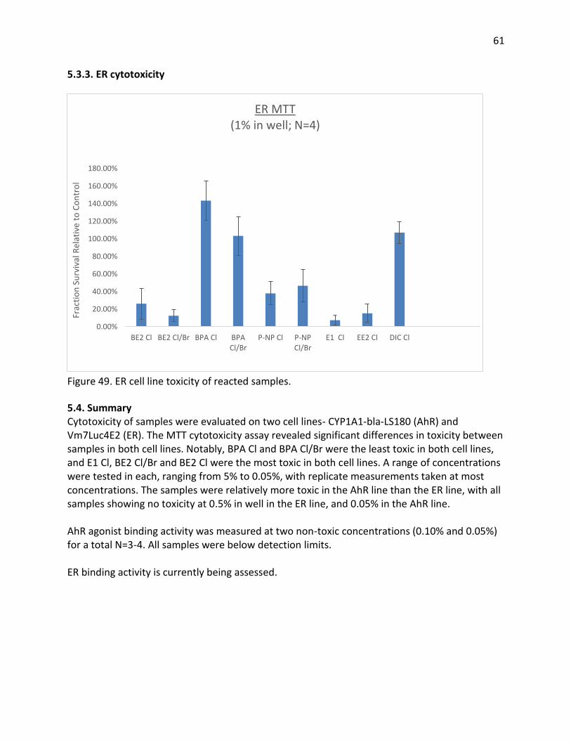
61

5.3.3. ER cytotoxicity

Figure 49. ER cell line toxicity of reacted samples. 5.4. Summary Cytotoxicity of samples were evaluated on two cell lines- CYP1A1-bla-LS180 (AhR) and Vm7Luc4E2 (ER). The MTT cytotoxicity assay revealed significant differences in toxicity between samples in both cell lines. Notably, BPA Cl and BPA Cl/Br were the least toxic in both cell lines, and E1 Cl, BE2 Cl/Br and BE2 Cl were the most toxic in both cell lines. A range of concentrations were tested in each, ranging from 5% to 0.05%, with replicate measurements taken at most concentrations. The samples were relatively more toxic in the AhR line than the ER line, with all samples showing no toxicity at 0.5% in well in the ER line, and 0.05% in the AhR line. AhR agonist binding activity was measured at two non-toxic concentrations (0.10% and 0.05%) for a total N=3-4. All samples were below detection limits. ER binding activity is currently being assessed.

0.00%

20.00%

40.00%

60.00%

80.00%

100.00%

120.00%

140.00%

160.00%

180.00%

BE2 Cl BE2 Cl/Br BPA Cl BPACl/Br

P-NP Cl P-NPCl/Br

E1 Cl EE2 Cl DIC Cl

Frac

tion

Surv

ival

Rel

ativ

e to

Con

trol

ER MTT(1% in well; N=4)

62

II. Scientific Presentations

Over the past year, the data generated in this study has been presented at several conferences. Kristin Cochran from USC has presented at three conferences since the last report; two presentations were poster presentations and one was an oral presentation. Ying Huang delivered an oral presentation at a conference. Dan Schlenk has a publication. See citations for details.

Citation: Removal and transformation of persistent priority emerging contaminants via advanced oxidation techniques and transformation product identification using mass spectrometry. Kristin H. Cochran, Jorge Casado, Danilo Russo, Danilo Spasiano, Marianna Vaccaro, Roberto Andreozzi, Raffaele Marotta, Nuno M. Reis, Gianluca Li Puma, Dionysios Dionysiou, Daniel Schlenk, and Susan D. Richardson. Southeast Regional Meeting of the American Chemical Society, Columbia, SC. Oct 23-26, 2016.

Citation: Removal and transformation of persistent emerging contaminants via advanced oxidation techniques and transformation product identification using mass spectrometry. Kristin H. Cochran, Jorge Casado, Danilo Russo, Danilo Spasiano, Marianna Vaccaro, Roberto Andreozzi, Raffaele Marotta, Nuno M. Reis, Gianluca Li Puma, Dionysios Dionysiou, Daniel Schlenk, and Susan D. Richardson. South Carolina Water Resources Conference, Columbia, SC. Oct 12-13, 2016.

Citation: Removal and transformation of persistent priority emerging contaminants via advanced oxidation techniques and transformation product identification using mass spectrometry. Kristin H. Cochran, Jorge Casado, Danilo Russo, Danilo Spasiano, Marianna Vaccaro, Roberto Andreozzi, Raffaele Marotta, Nuno M. Reis, Gianluca Li Puma, Dionysios Dionysiou, Daniel Schlenk, and Susan D. Richardson. South Carolina Environmental Conference, Myrtle Beach, SC. March 12-15, 2017. Citation: Treatment of emerging contaminants in water reuse applications. Yiqing Liu, Ying Huang, Susan D. Richardson, and Dionysios D. Dionysiou. Advanced Oxidation Technologies for Treatment of Water, Air, and Soil conference (AOTs-22), Atlanta, GA. Nov 13-17, 2016. Citation: Pflug, NC., Kupsco, A., Kolodziej, EP., Schlenk, D., Teesch, LM., Gloer, JB., Cwiertny, DM. (2017). Formation of bioactive transformation products during glucocorticoid chlorination. Water Research and Technology 3(3): 450-461.

63

III. Next Steps

USC. Continue spiked recovery experiments to optimize SPE method and check breakthrough, as well as increase concentration factor while keeping sample volumes reasonable. Add two more compounds (NDMA and chloropyrifos) into the method and optimize LC-MS parameters for them. Identify transformation products from AOTs done at University of Cincinnati. Improve sensitivity of Waters LC/MS for better quantification. Finish processing chlorination and chlorination/bromination reactions for transformation product identification. The GC/MS method will be optimized for the remaining compounds. Two more sampling events are coming up this year, one in August and one in October. Quantification of the entire list of 21 ECs will be done during these events, as well as transformation product identification and analysis for disinfection by-products. We would also like to do spiked recovery experiments in GWRS waters rather than relying on comparability to our local wastewater.

UC-Riverside. Assess ER binding activity and compare halogenated compound toxicity with the toxicity of the parent compound. Also analyze more AOP treated samples, preferably at a higher concentration. Analyze toxicity of April GWRS sampling (unreacted water and reacted water – chlorination and chlorination/bromination). Univ. of Cincinnati. For the UC team, we are planning to study the degradation of the mixture of five CEC using UV-C/H2O2 and solar light/TiO2 in field water matrix for two more sample events. Cytotoxicity study of the photocatalytic treated water will be examined at all the experimental scenarios. Also, the transformation by-products will also be examined and identified for the individual contaminants using LC-MS-MS and/or GC-MS.

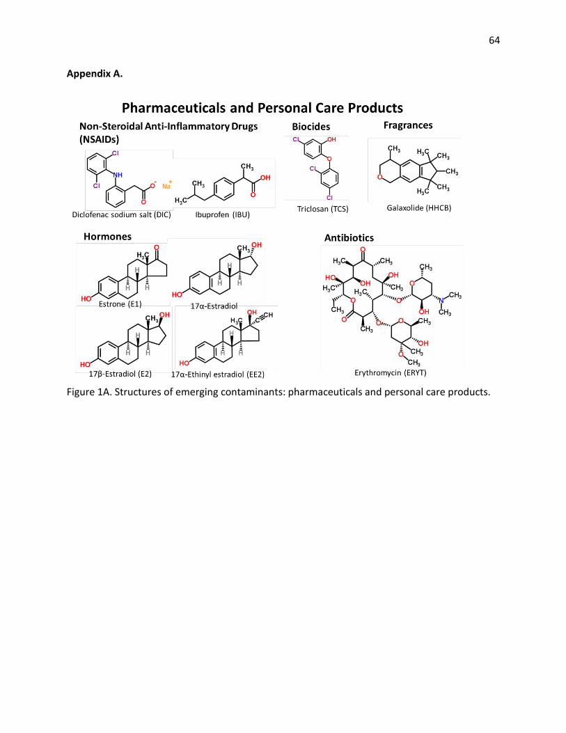
64

Appendix A.

Figure 1A. Structures of emerging contaminants: pharmaceuticals and personal care products.

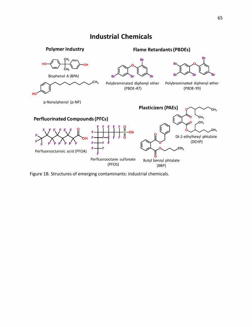
65

Figure 1B. Structures of emerging contaminants: industrial chemicals.

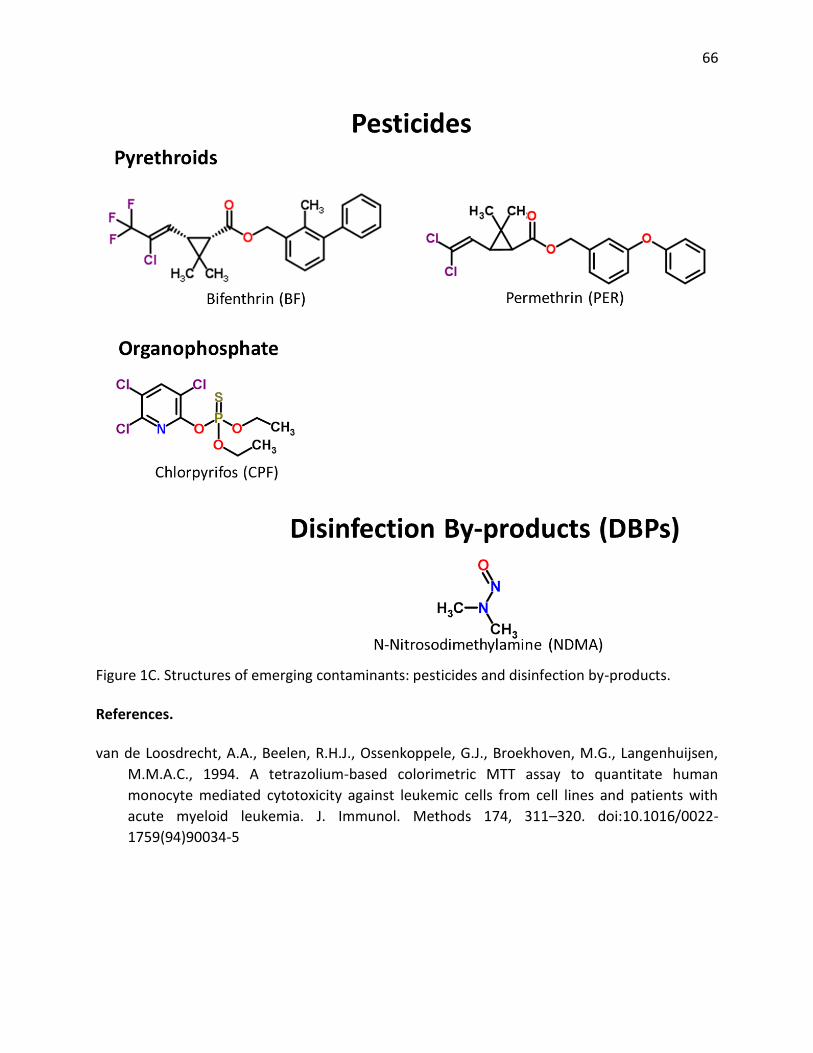
66

Figure 1C. Structures of emerging contaminants: pesticides and disinfection by-products. References. van de Loosdrecht, A.A., Beelen, R.H.J., Ossenkoppele, G.J., Broekhoven, M.G., Langenhuijsen,

M.M.A.C., 1994. A tetrazolium-based colorimetric MTT assay to quantitate human monocyte mediated cytotoxicity against leukemic cells from cell lines and patients with acute myeloid leukemia. J. Immunol. Methods 174, 311–320. doi:10.1016/0022-1759(94)90034-5

The Influence of Poultry Rearing Facilities on NutrientConcentrations, Fecal Indicator Bacteria, and Stream Fishin the Upper Savannah River Basin

Basic Information

Title: The Influence of Poultry Rearing Facilities on Nutrient Concentrations, Fecal IndicatorBacteria, and Stream Fish in the Upper Savannah River Basin

Project Number: 2016SC103BStart Date: 5/1/2016End Date: 5/1/2017

Funding Source: 104BCongressional

District: SC-004

ResearchCategory: Water Quality

Focus Categories: Water Quality, Non Point Pollution, AgricultureDescriptors: None

PrincipalInvestigators: Gregory Paul Lewis, Dennis C. Haney, Peter Van Den Hurk, MinKen Liao

Publications


The Influence of Poultry Rearing Facilities on Nutrient Concentrations, Fecal Indicator Bacteria, and Stream Fish in the Upper Savannah River Basin

The Influence of Poultry Rearing Facilities on Nutrient Concentrations, Fecal Indicator Bacteria, and Stream Fish in the Upper Savannah River Basin1

1

The Influence of Poultry Rearing Facilities on Nutrient Concentrations, Fecal Indicator Bacteria, and Stream Fish in the Upper Savannah River Basin Summary of Preliminary Results, 31 May 2017 Principal Investigators: Gregory P. Lewis, Ph.D., Professor, Department of Biology, Furman University, 3300 Poinsett Highway, Greenville, SC 29613. Phone: 864.294.3249. [email protected] Dennis C. Haney, Ph.D., Professor and Chair, Department of Biology, Furman University, 3300 Poinsett Highway, Greenville, SC 29613. Phone: 864.294.2050. [email protected] Min-Ken Liao, Ph.D., Professor, Department of Biology, Furman University, 3300 Poinsett Highway, Greenville, SC 29613. Phone: 864.294.3246. [email protected] Peter van den Hurk, Ph.D., Associate Professor. Department of Biological Sciences, Clemson University, 132 Long Hall, Clemson, SC 29634. Phone: 864.656.3594. [email protected] Summary of Sampling and Data Collection: Our primary research goal was to evaluate possible effects of poultry rearing facilities on nutrient concentrations, fecal indicator bacteria, and fish communities in rural watersheds of the upper Savannah River Basin of South Carolina (Oconee and Anderson Counties). During June-August 2016, we collected data from 28 sampling sites on first to third order streams in the upper Savannah River basin within the South Carolina Piedmont. We collected water samples at least twice from each stream for chemical and bacterial analyses. Fish were sampled at 18 of the sites using a backpack electrofisher and seine. Passive (POCIS disk) samplers were deployed at 7 of the sites from summer to autumn to test for the presence of pharmaceutical compounds (including antibiotics) in stream water. Student Involvement: Another major goal of the project was to provide research training for students. Students were involved closely in all aspects of the project, including sample site selection, field sampling, laboratory analyses, and data analyses. The project involved work by three undergraduate Biology majors from Furman University (Cullen Carter, Utkarsh (Kumar) Mishra, and Jocelyn Stalker), one high school student from the South Carolina Governor's School for Science and Mathematics (Savannah League), and a master’s student from the Department of Biological Sciences at Clemson University (David Wyker). Conference Presentations and Abstracts: As of May 2017, four conference presentations have been given which included results of the project. Below we provide the abstracts from these presentations as a summary of our initial data analyses. Three of the presentations also incorporated data from stream samplings funded

2

by a previous grant to our research group from USGS through the South Carolina Water Resources Center. The first three presentations were made at the annual meeting of the Association of Southeastern Biologists in Montgomery, Alabama, April 2017 (names of undergraduate students indicated with asterisks): 1. Cullen M. Carter*, Gregory P. Lewis, Min-Ken Liao, Dennis C. Haney, Kumar Mishra*, and Jocelyn B. Stalker*. "Relationships between poultry farms and suspended bacteria in streams of the South Carolina Piedmont" (poster presentation) Previous studies provide evidence that poultry farms influence water quality in streams and rivers in some regions. In particular, farms may be sources of fecal bacteria and nutrients to streams. Chronic treatment of poultry with antibiotics may also lead to inputs of antibiotic-resistant bacteria from farms to water bodies. We examined whether chicken farms in the western Piedmont of South Carolina influenced the abundance of suspended bacteria in streams of the Upper Savannah River Basin. We hypothesized that the concentrations of both fecal indicator bacteria and total heterotrophic bacteria in small streams would correlate positively with the density of chicken houses in the streams’ watersheds. During June-August 2016, under drought conditions, we collected water samples from 28 sites on first to third order streams. Land cover in the streams’ watersheds ranged from mostly forested to mixtures of pasture, forest, and row crops. Chicken house densities ranged from 0 to 7.7 houses/km2. We measured concentrations of total coliforms and Escherichia coli, tetracycline-resistant total coliforms and E. coli, Enterococcus, and total heterotrophic bacteria. Water samples also were analyzed for turbidity, major ions, total dissolved nitrogen, and dissolved organic carbon (DOC). In simple bivariate correlations, concentrations of total coliforms and E. coli (including tetracycline-resistant coliforms and E. coli) correlated positively with chicken house density. However, after accounting for variation in watershed pasture cover with partial correlation analyses, these correlations were not significant. Concentrations of Enterococcus and total heterotrophic bacteria did not correlate significantly with chicken house density, but total heterotroph concentrations correlated positively with DOC concentrations. The drought conditions under which we conducted our study may have minimized impacts of poultry farms on bacteria concentrations. Additional research will be needed to better separate the influence of poultry farms and pasture on bacterial abundance in streams of this region. 2. Gregory P. Lewis, Dennis C. Haney, Min-Ken Liao, and Peter van den Hurk. "Relationships between land cover/land use, nutrient concentrations, and turbidity of headwater streams in the South Carolina Piedmont" (oral presentation)

3

In recent decades, the Piedmont region of the southeastern United States has experienced rapid land transformation, especially with the expansion of urban areas into rural landscapes. Nonetheless, rural land covers and land uses, including forested and agricultural lands, remain widespread. Therefore, it is important to understand how various land covers and land uses influence water quality in drainage waters in the region. Between 2011 and 2016, we sampled 79 first to fourth order streams in the South Carolina Piedmont under baseflow conditions. These streams included 10 streams in heavily urbanized watersheds. The remaining streams drained rural watersheds ranging from completely forested to those with varying mixtures of forest, pasture, and/or row crops. Poultry farms were located within some of the rural watersheds, as well. Water samples from all streams were analyzed for major ions, total dissolved nitrogen (TDN), dissolved organic carbon, and turbidity. Among rural streams with negligible (<1.5%) crop cover and no poultry farms, TDN concentrations correlated positively with percent of watershed area in pasture. However, turbidity did not correlate with pasture cover. Streams in “agricultural” watersheds with pasture and row crops and/or poultry farms had the highest TDN concentrations and turbidity. Streams draining watersheds with >80% forest cover and no poultry farms had the lowest TDN concentrations. The lowest turbidities tended to occur in streams draining heavily forested or urban watersheds. Nitrite and phosphate concentrations were typically near or below our detection limit in most streams but were elevated in some watersheds with pasture and/or crop cover. Our results suggest that, in the South Carolina Piedmont, even small areas of row crops and the presence of poultry farms in rural watersheds can result in stream nitrogen (and in some cases phosphate) concentrations that equal or exceed concentrations in highly urbanized watersheds. 3. Jocelyn B. Stalker*, Dennis C. Haney, Kumar Mishra*, Cullen Carter*, and Gregory P. Lewis. "The influence of poultry rearing facilities on streams and stream fish in the Upper Savannah River Basin" (oral presentation) In the South Carolina Piedmont, human influences on water quality and stream organisms are widespread, with streams in this region typically possessing low fish diversity compared to streams elsewhere in the southeastern United States. Most previous studies have focused on the effects of humans on urban streams, with these urban areas being influenced by extensive roadways, travel emissions, and land use change due to urban sprawl. Studies have also suggested that humans influence rural streams as well, though the sources of influence are different. Rural areas in SC are frequently covered by farmland, including both pasture and row crop agriculture, and some areas, especially in Oconee County, feature high densities of poultry rearing facilities (PRFs). As such, during May-August 2016 we studied fish diversity and abundance, geomorphology, water quality, and habitat quality in streams downstream of PRFs to explore the effects of this form of land use on rural streams in this area. Data were compared to that from previous studies we have conducted that examined pasture, row crop agriculture, and forested land covers at sites lacking PRFs. Results suggest that PRFs may actually increase fish

4

diversity, species richness, and overall biotic quality at sites where the predominant land cover is pasture, possibly because these sites also had higher levels of nitrogenous chemical nutrients. In contrast, sites with PRFs that were predominantly forested or agricultural had lower fish abundance. It could be that pastured land covers are more likely to be influenced by PRFs since chicken litter is most commonly spread on fields, though further studies will be needed to confirm such effects. This information can help SC shape its farming and agricultural practices to preserve the ecological integrity of rural streams while also protecting human health by maintaining clean and safe water sources. The fourth presentation was made at the annual European meeting of the Society of Environmental Toxicology and Chemistry (SETAC) in Brussels, Belgium, May 2017 (name of master's student indicated with an asterisk). 4. Peter van den Hurk, David Wyker*, Dennis Haney, and Greg Lewis. " Biological effects monitoring and passive samplers as chemical pollution monitoring devices in the Savannah River basin, USA" (poster presentation) The Savannah River watershed stretches from North Carolina down the foothills of the Southern Appalachian Mountains towards to the Atlantic Ocean near Savannah, GA. The Savannah River is about 300 miles long and drains a basin of almost 10,000 sq. miles. This makes it one of the major rivers in the southeastern USA. The upper half of the Savannah River watershed is dominated by several smaller and larger reservoirs. Below these reservoirs several smaller dams are located around the city of Augusta, followed by a basically unobstructed navigable river that connects the Augusta area to the open ocean. In the upper part of the watershed, mostly in Oconee and Anderson counties, smaller tributaries to the Savannah River flow through areas that are intensively used by poultry industry. The lower part of the river, starting around the city of Augusta, receives effluents from a variety of sources, like wastewater treatment plants, chemical industries, a paper mill, a nuclear testing facility, and urban runoff. Two projects were initiated over the last few years to investigate the effects of these pollution sources on aquatic biota in the Savannah River basin. For the chemical monitoring we selected a passive sampler approach, which gives a more time integrated picture of chemical contamination than grab samples at fixed time points. The results of our analysis of these passive samplers shows that in the upper basin, in which we mostly focused on effects of poultry farming, a variety of human and veterinarian pharmaceuticals are found in the streams. Most abundant among the human drugs are

5

carbamazepine, erythromycin and trimethoprim. Most veterinary drugs were ionophores, like monensin and nigericin. In the lower Savannah River we looked at several human pharmaceuticals, estrogens, a flame retardant, PCBs and PAHs as indicators for effluents of different sources. While biological effect monitoring showed only minor disturbances in most locations, the chemical analysis of the passive samplers demonstrates that the chemical footprint of human activities are widespread in the Savannah River basin. Nevertheless, while biomarker results were only significant in a few locations, compound specific effects on aquatic organisms, like endocrine disruption, may be more widespread than was observed in this study.

Monitoring of Organic Pollutants in the Savannah, Edistoand Ogeechee Rivers, using Passive Samplers inCombination with a Real-Time Water Quality Data CollectionNetwork

Basic Information

Title:Monitoring of Organic Pollutants in the Savannah, Edisto and Ogeechee Rivers, usingPassive Samplers in Combination with a Real-Time Water Quality Data CollectionNetwork

Project Number: 2016SC104BStart Date: 5/1/2016End Date: 4/30/2017

Funding Source: 104BCongressional

District: SC-003

ResearchCategory: Water Quality

Focus Categories: Water Quality, Toxic Substances, MethodsDescriptors: None

PrincipalInvestigators: Peter Van Den Hurk, Oscar Paul Flite

Publications


Monitoring of Organic Pollutants in the Savannah, Edisto and Ogeechee Rivers, using Passive Samplers in Combination with a Real-Time Water Quality Data Collection Network

Monitoring of Organic Pollutants in the Savannah, Edisto and Ogeechee Rivers, using Passive Samplers in Combination with a Real-Time Water Quality Data Collection Network1

MonitoringoforganicpollutantsintheSavannah,EdistoandOgeecheeRivers,usingpassivesamplersincombinationwithareal-timewater

qualitydatacollectionnetwork.

PetervandenHurk,OscarP.FliteIII,DavidWyker

2016-2017ProgressReportforthe

SouthCarolinaWaterResourcesCenter

TheSavannahRiverwatershedstretchesfromNorthCarolinadownthefoothillsoftheSouthernAppalachianMountainstowardstotheAtlanticOceannearSavannah,GA.TheSavannahRiverisabout300mileslonganddrainsabasinofalmost10,000sq.miles.ThismakesitoneofthemajorriversinthesoutheasternUSA.TheupperhalfoftheSavannahRiverwatershedisdominatedbyseveralsmallerandlargerreservoirs.BelowthesereservoirstwosmallerdamsarelocatedaroundthecityofAugusta,followedbyabasicallyunobstructednavigableriverthatconnectstheAugustaareatotheopenocean.

Intheupperpartofthewatershed,mostlyinOconeeandAndersoncounties,smallertributariestotheSavannahRiverflowthroughareasthatareintensivelyusedbypoultryindustry.Inaddition,alegacyproblemwithPCBsfromtheSangamoplantinPickens,andruraleffluentsfromsmallerwastewatertreatmentplantsandsepticsystemspotentiallyaffectwaterqualityintheSavannahRivertributaries.Thelowerpartoftheriver,startingaroundthecityofAugusta,receiveseffluentsfromavarietyofsources,likewastewatertreatmentplants,chemicalindustries,apapermill,anucleartestingfacility,andurbanrunoff.

Toimplementachemicalandbiologicaleffectsmonitoringstrategyweselectedapassivesamplerapproach,whichgivesamoretimeintegratedpictureofchemicalcontaminationthangrabsamplesatfixedtimepoints.ContinuoussamplingofthreelocationsalongtheSavannahRiveraswellaswithinStromThurmondandHartwellDamshasbeenperformedoverthelasttwoandahalfyears.Morerecently,continuoussamplingintheOgeecheeandEdistoRivershavebeenundertakenwiththeassistanceofthePhinizyCenterfortheWaterSciences.Samplinghasbeenperformedwiththeuseofpassivesamplingdevicesthatareleftoutforextendedperiodsoftimetoconcentratecompoundspresentinthesurfacewaters,allowingforimprovedchemicalanalyses.Samplesobtainedfromthesesitesarebeinganalyzedfor6pharmaceuticals/personalcareproducts(PPCPs),3estrogens(endocrinedisruptors),andtheEPApriority16PAHs(toxiccombustionbyproducts).LimitedanalysisonSavannahRiversampleswasalsoperformedforPCB’s(polychlorinatedbiphenyls),alegacycontaminantreleasedfromtheSangamoWestonSuperfundsiteintheTwelveMileCreek/LakeHartwellarea.

AttheSavannahRiversitelocations(RM190,RM179,RM119),respectivelysituateddownstreamofAugusta,allPPCPsbeingmonitoredweredetected.LevelsofthesedrugsintheSavannahRiversurfacewatersareestimatedtobeng/Ltosub-ng/Lconcentrations,individually.Theseareallbelowknownphysiologicallyrelevantconcentrations.Forindividualcompounds,concentrationsandpatternsalongthesamplingareadiffer.Concentrationsarerelativelysimilarforeachcompoundas

samplingmovesdownstream,thoughsomecompoundsdisplayspatialtrendspotentiallyattributabletodifferinglanduse.Flowrate,directlyrelatedtoriverdischarge,caninfluencetheuptakeofcompoundsontothePSD.DischargedataobtainedfromtheUSGSsitejustnorthofSavannahRivermile190doesnotshowasignificanteffectofflowrateonconcentration.ThissuggeststhatspikesinPPCPsareduetoincreasedusageofthedrugs,potentiallyrelatedtoseasonaltrendssuchasthoseseeninantihistamines(allergydrugs).ConcentrationsofthedrugsfoundinthesurfacewatersofGeorgiaandSouthCarolinaarereflectingthelocalPPCPconsumption.Limitedanalysesofestrogens,bothnaturalandsynthetic,areshowinglowconcentrations,withmostsitesbelowthedetectablelimit.Thisconfirmsearlierresultsobtainedusingbioassaystoassesstotalestrogenicityofthecollectedsurfacewatersamples.

ThelimitedPCBanalysisperformedfortheSavannahRiversitesshowsatrendsimilartootherfindings.PCBconcentrationsincreasefurtherdownstreamofthesourcewiththehighestconcentrationsmeasuredatRM119,andthelowestatRM190.PCBsgenerallyassociatewiththeriversedimentandarelikelyslowlymovingdownstreamwiththesediment.PCBstendnottostaywithinthewatercolumnwhichisreflectedinthelowconcentrationsmeasuredinthesurfacewaters.TotalPCBconcentration,whichisatotalof128individualPCBs,rangedbetween5-12ngPCBTOT/gPSD.Averagesurfacewaterconcentrationshavenotcurrentlybeendetermined.PAHanalysiscompletedsofarpotentiallydepictssignificanttemporalandspatialdifferences,ranginginconcentrationbetween~80-1100ppbtotalPAH.Analysiswillbecompletedwithinthemonthatwhichpointthesetrendswillbemoreclearlyunderstood.

AnalysisofsamplesobtainedwithintheStromThurmondandHartwellDamsdisplayedsimilartrendswithPPCPsandestrogens.SamplesfromthedamsthoughhadloweroveralllevelsofPPCPs.HigherlevelsofallcompoundswerepresentatthesitesfurthersoutharoundthemoreurbanAugustaarea.Betweenthetwodamlocations,thelowestconcentrationsofPPCPswerepresentatStromThurmond,withtheexceptionofTrimethoprimwhichwassimilaratbothsites.Waterflowismaintainedataconstantratewithinthedamsandsochangesinriverdischargeshouldnotinfluencetheseresults.

TheOgeecheeandEdistoRiversaresmallerwaterwayslocatedinGeorgiaandSouthCarolina,respectively.EarlysamplesfromtheOgeecheeRiverwerelostandrecentsamplesarestilltobeanalyzed.SamplesanalyzedfromtheEdistoRiverhavethelowestPPCPconcentrationsofallthesamples.NeitherTrimethoprimnorCarbamazepineweredetectedattheEdistolocation.Ageneraloverviewofthesampledsitessuggeststhedegreeofdevelopmentintheareaistheprimarycomponentinfluencingcontaminantconcentrations.Othervariablesinfluencetrendsincontaminantconcentrations,includingobservedtemporaltrends,andwillbethesubjectoffurtherstudy.

TheprojecthassupportedaPh.D.student(DavidWyker),andresultshavebeenpresentedattheSETACN.AmericameetinginOrlando(Nov.2016)andSETACEuropemeetinginBrussels(May2017).

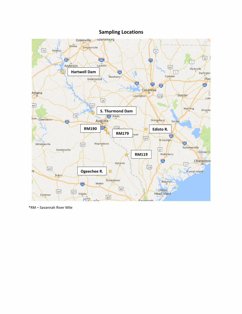
SamplingLocations

*RM–SavannahRiverMile

HartwellDam

S.ThurmondDam

RM190RM179

RM119

OgeecheeR.

EdistoR.

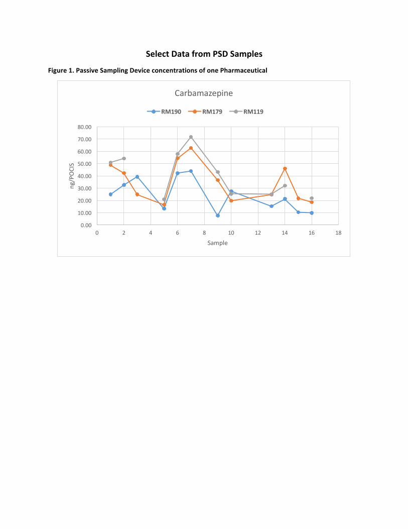
SelectDatafromPSDSamples

Figure1.PassiveSamplingDeviceconcentrationsofonePharmaceutical

0.00

10.00

20.00

30.00

40.00

50.00

60.00

70.00

80.00

0 2 4 6 8 10 12 14 16 18

ng/POCIS

Sample

Carbamazepine

RM190 RM179 RM119

Information Transfer Program Introduction

None

Information Transfer Program Introduction

Information Transfer Program Introduction 1

USGS Summer Intern Program

None.

USGS Summer Intern Program 1

Student Support

Category Section 104 BaseGrant

Section 104 NCGPAward

NIWR-USGSInternship

SupplementalAwards Total

Undergraduate 0 0 0 0 0Masters 1 0 0 0 1

Ph.D. 1 3 0 0 4Post-Doc. 0 0 0 0 0

Total 2 3 0 0 5

1

Notable Awards and Achievements

Completed writing the policy and management chapter for the South Carolina Storm-water Pond State of theKnowledge Report – will be published by the S.C. Sea Grant Consortium

Completed work on funded project to conduct stakeholder engagement meetings for the SCDNR sponsoredSouth Carolina River Basin Surface Water Assessment.

Secured additional funding for the SCDNR sponsored South Carolina Groundwater Assessment to conductstakeholder meetings

Received funding through U.S. Department of Agriculture for a project to analyze land use changes andassociated water consumption using multiple remote sensing platforms in the Savannah River Basin

Continued work on funding from U.S. Army Corps of Engineers to conduct an economic analysis of changesto flow regimes in the lower Savannah River Basin

Successfully conducted SCWRC statewide research solicitation under the guidelines of USGS.

Served as chairman of the Planning Committee of the S.C. Water Resources Conference

Served on editorial committee for the Journal of South Carolina Water Resources

Planned workshop with SC Water Resources Conference Planning Committee on drought and droughtresponse by state agencies in S.C.

Served on the Savannah River Basin Advisory Council.

Served on the Carolinas Integrated Sciences & Assessments Advisory Board

Served on the SC Sea Grant Consortium Coastal Communities Advisory Board

Served on SCDNR State Water Plan Advisory Committee

Served on the SC Sea Grant Consortium Program Advisory Board

Served on the Science Advisory Committee of the Catawba Wateree Water Management Group

Served on the Selection Committee of the Duke Energy Water Fund

Served on the Science Advisory Committee of the Savannah River Clean Water Fund

The 2016 S.C. Water Resources Conference, sponsored by the S.C. Water Resources Center: 350 Participants100 Groups represented 44 Students 108 Oral presentations 46 Posters on display 23 Exhibitors 9 Majorfinancial contributors 11 Supporting financial contributors

The 2016 S.C. Water Resources Conference, sponsored by the S.C. Water Resources Center – MediaCoverage: 1,400,000 Impacts from earned print and broadcast media 9,274 Unique visitors to web site 4,300@SCWaterNews Twitter impressions for October 200 Online viewers for plenary sessions

Notable Awards and Achievements 1

South Carolina Water Resources Center Annual Technical ... · South Carolina Water Resources Center...

Documents

Transcript of South Carolina Water Resources Center Annual Technical ... · South Carolina Water Resources Center...