Journal of Computational Physics 230 (2011) 2677–2695

Contents lists available at ScienceDirect

Journal of Computational Physics

journal homepage: www.elsevier .com/locate / jcp

Sources of spurious force oscillations from an immersed boundarymethod for moving-body problems

Jongho Lee a, Jungwoo Kim b, Haecheon Choi a,⇑, Kyung-Soo Yang c

a School of Mechanical and Aerospace Engineering, Seoul National University, San 56-1 Sillim-dong, Gwanak-gu, Seoul 151-744, Republic of Koreab Nuclear Research Safety Department, Korea Atomic Energy Research Institute, Yuseong, Daejeon 305-353, Republic of Koreac Department of Mechanical Engineering, Inha University, Incheon 402-751, Republic of Korea

a r t i c l e i n f o

Article history:Received 19 February 2010Received in revised form 24 December 2010Accepted 4 January 2011Available online 13 January 2011

Keywords:Immersed boundary methodMoving bodySpurious force oscillationsPressure discontinuityVelocity discontinuity

0021-9991/$ - see front matter � 2011 Elsevier Incdoi:10.1016/j.jcp.2011.01.004

⇑ Corresponding author. Also at: Institute of AdvaE-mail address: choi@snu.ac.kr (H. Choi).

a b s t r a c t

When a discrete-forcing immersed boundary method is applied to moving-body problems,it produces spurious force oscillations on a solid body. In the present study, we identify twosources of these force oscillations. One source is from the spatial discontinuity in the pres-sure across the immersed boundary when a grid point located inside a solid body becomesthat of fluid with a body motion. The addition of mass source/sink together with momen-tum forcing proposed by Kim et al. [J. Kim, D. Kim, H. Choi, An immersed-boundary finitevolume method for simulations of flow in complex geometries, Journal of ComputationalPhysics 171 (2001) 132–150] reduces the spurious force oscillations by alleviating thispressure discontinuity. The other source is from the temporal discontinuity in the velocityat the grid points where fluid becomes solid with a body motion. The magnitude of velocitydiscontinuity decreases with decreasing the grid spacing near the immersed boundary.Four moving-body problems are simulated by varying the grid spacing at a fixed computa-tional time step and at a constant CFL number, respectively. It is found that the spuriousforce oscillations decrease with decreasing the grid spacing and increasing the computa-tional time step size, but they depend more on the grid spacing than on the computationaltime step size.

� 2011 Elsevier Inc. All rights reserved.

1. Introduction

One of important issues in computational fluid dynamics is how to accurately and efficiently solve the flow problemsassociated with moving bodies in a fluid. In case the body shape is complicated, one of possible numerical methods to dealwith the complex geometry may be an immersed boundary method (see, e.g. [1–15]). This method has been successfullyapplied to various complex flows including stationary and moving bodies [16].

When an immersed boundary (called IB hereafter) method is used for moving-body problems, it greatly saves the com-putational cost because re-meshing is in principle not required. Although it has been rarely mentioned, however, it is knownthat there exist spurious force oscillations (called SFOs hereafter) on a solid body when a discrete-forcing IB method isapplied to moving-body problems in an inertial reference frame (see, e.g. [12,13]). These SFOs degrade the quality of solu-tions and thus it is desirable to reduce them as much as possible. For single-body problems, it is possible to use a non-inertialreference frame (i.e. fixing the coordinate to a solid body) in conjunction with an IB method [17], with which the SFOs arecompletely eliminated. However, this approach is not possible for multiple moving-body problems.

. All rights reserved.

nced Machinery and Design, Seoul National University, Republic of Korea.

2678 J. Lee et al. / Journal of Computational Physics 230 (2011) 2677–2695

As mentioned above, there have been only a few studies on this issue in the literature. Uhlmann [12] introduced a methodof attenuating the SFOs by combining the regularized delta function of Peskin [9] and the discrete (or direct) forcing methodof Fadlun et al. [6]. Yang and Balaras [13] suggested a ‘field extension’ approach to reduce the SFOs, in which the velocity andpressure at the grid points where solid becomes fluid due to a body motion were obtained by an extrapolation from adjacentfluid grid points. These methods effectively reduced the SFOs but did not completely eliminate them. Therefore, it is requiredto identify the sources of these force oscillations for more reliable solutions from a discrete-forcing IB method for moving-body problems.

In the present study, we use an IB method developed by Kim et al. [7] to identify the sources of SFOs for moving-bodyproblems. The results obtained in this study should be also valid for other discrete-forcing IB methods (e.g. [6,10,11],etc.). We consider four moving-body problems such as the horizontal oscillation of a square cylinder, in-line and cross-flowoscillations of a circular cylinder, and a wing flapping motion. Different grid spacings and computational time step sizes aretested for these moving-body problems. In Section 2, the numerical method used is presented. Section 3 shows two sourcesof SFOs. Numerical examples are given in Section 4, followed by a conclusion in Section 5.

2. Numerical method

2.1. Governing equations

The governing equations for unsteady incompressible flow in an inertial reference frame using the IB method by Kim et al.[7] are

@ui

@tþ @uiuj

@xj¼ � @p

@xiþ 1

Re@2ui

@xj@xjþ fi; ð1Þ

@ui

@xi� q ¼ 0; ð2Þ

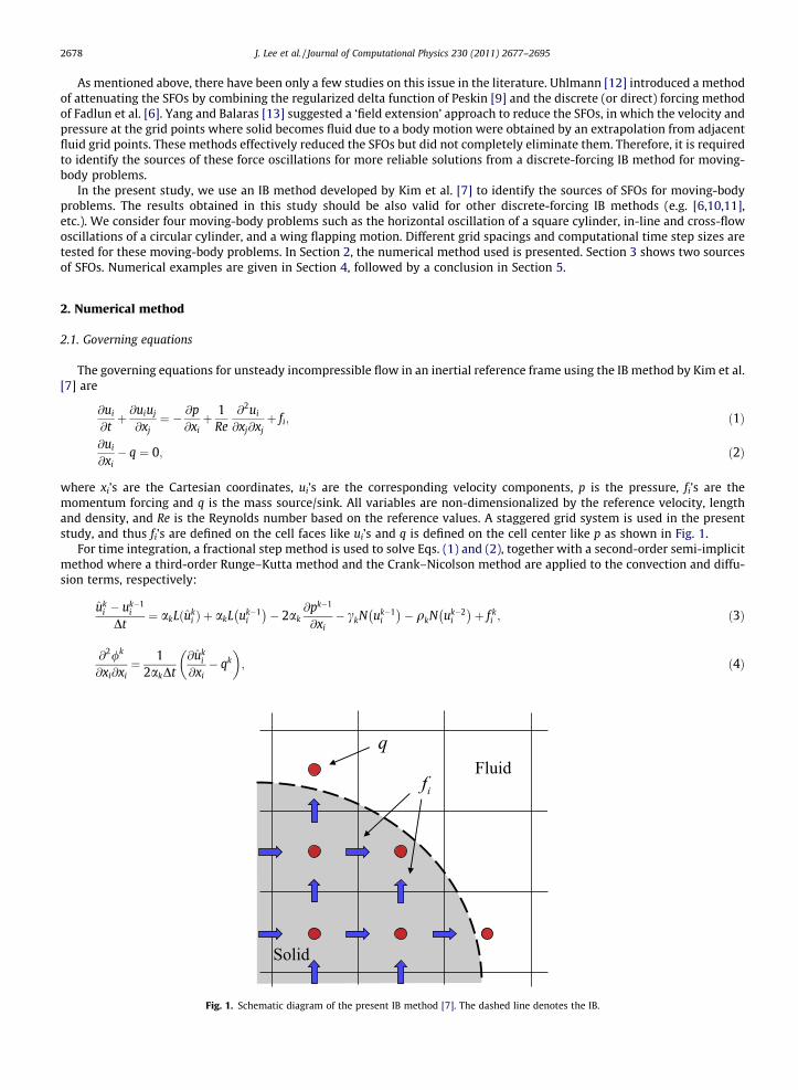
where xi’s are the Cartesian coordinates, ui’s are the corresponding velocity components, p is the pressure, fi’s are themomentum forcing and q is the mass source/sink. All variables are non-dimensionalized by the reference velocity, lengthand density, and Re is the Reynolds number based on the reference values. A staggered grid system is used in the presentstudy, and thus fi’s are defined on the cell faces like ui’s and q is defined on the cell center like p as shown in Fig. 1.

For time integration, a fractional step method is used to solve Eqs. (1) and (2), together with a second-order semi-implicitmethod where a third-order Runge–Kutta method and the Crank–Nicolson method are applied to the convection and diffu-sion terms, respectively:

uki � uk�1

i

Dt¼ akLðuk

i Þ þ akL uk�1i

� �� 2ak

@pk�1

@xi� ckN uk�1

i

� �� qkN uk�2

i

� �þ f k

i ; ð3Þ

@2/k

@xi@xi¼ 1

2akDt@uk

i

@xi� qk

� �; ð4Þ

Fig. 1. Schematic diagram of the present IB method [7]. The dashed line denotes the IB.

Fig

J. Lee et al. / Journal of Computational Physics 230 (2011) 2677–2695 2679

uki ¼ uk

i � 2akDt@/k

@xi; ð5Þ

pk ¼ pk�1 þ /k � akDtRe

@2/k

@xj@xj; ð6Þ

where Lðuki Þ ¼ 1

Re@2uk

i@xj@xj

, Nðuki Þ ¼

@ukiuk

j

@xj, ui’s are the intermediate velocity, / is the pseudo-pressure, Dt is the computational time

step, and k is the sub-step index (k = 1,2,3), respectively. ak, ck and qk are the coefficients for the sub-steps: a1 = 4/15, c1 = 8/15, q1 = 0; a2 = 1/15, c2 = 5/12, q2 = �17/60; a3 = 1/6, c3 = 3/4, q3 = �5/12. The second-order central difference scheme is ap-plied to all the spatial derivatives. The momentum forcing fi is determined by the following equation (the detailed procedureof obtaining fi and q is described in detail in [7] and thus we do not repeat it here):

f ki ¼

Uki � uk�1

i

Dt� 2akL uk�1

i

� �þ 2ak

@pk�1

@xiþ ckN uk�1

i

� �þ qkN uk�2

i

� �; ð7Þ

where Uki ’s are the desired velocities at the grid points where f k

i ’s are applied, and are obtained by the linear or bilinear inter-polation (trilinear interpolation for three dimensional case) from ~uk

i ’s. Here ~uki ’s are the provisional velocities in the fluid re-

gion near the IB updated by an explicit time integration scheme with f ki ¼ 0:

~uki � uk�1

i

Dt¼ 2akL uk�1

i

� �� 2ak

@pk�1

@xi� ckN uk�1

i

� �� qkN uk�2

i

� �: ð8Þ

2.2. Calculation of the force on a solid body

Fig. 2 shows the schematic diagram for the calculation of the force on a solid body, where CV1 and CV2 denote the controlvolumes for solid and fluid, respectively, and CV3 = CV1 + CV2. Fi is the force acting on the solid body and Fo,i is the force on theouter boundary of CV3.

The force Fi on CS1 (control surface of CV1) is obtained by integrating the Navier–Stokes equation over CV2 as follows:

Fi ¼ �Z

CS1

�pni þ1Re

@ui

@xjþ @uj

@xi

� �nj

� �dS ¼

ZCS3

�pni þ1Re

@ui

@xjþ @uj

@xi

� �nj

� �dS�

ZCV2

@ui

@tþ @uiuj

@xj

� �dV

¼ Fo;i �Z

CV2

@ui

@tþ @uiuj

@xj

� �dV ¼ Fo;i �

ZCV3

@ui

@tþ @uiuj

@xj

� �dV þ

ZCV1

@ui

@tþ @uiuj

@xj

� �dV : ð9Þ

Integrating the Navier–Stokes equation over CV3 and using the Gauss theorem, the second term in the right hand side of Eq.(9) becomes

Z

CV3

@ui

@tþ @uiuj

@xj

� �dV ¼

ZCV3

� @p@xiþ 1

Re@2ui

@xj@xj

!dV þ

ZCV3

fi dV

¼Z

CS3

�pni þ1Re

@ui

@xjþ @uj

@xi

� �nj

� �dS� 1

Re

ZCS3

@uj

@xinj dSþ

ZCV3

fi dV

¼ Fo;i �1Re

ZCV3

@

@xj

@uj

@xi

� �dV þ

ZCV3

fi dV ¼ Fo;i �1Re

ZCS3

@uj

@xjni dSþ

ZCV3

fi dV

¼ Fo;i þZ

CV1

fi dV ; ð10Þ

. 2. Schematic diagram for the calculation of the force on a solid body. The dashed lines denote the inner and outer control surfaces of CV2.

2680 J. Lee et al. / Journal of Computational Physics 230 (2011) 2677–2695

where CS3 is the control surface of CV3, andR

CS3

@uj

@xjni dS ¼

RCS3

qni dS ¼ 0 because q = 0 on CS3. Then, Eq. (9) becomes

Fig. 3.is the v

Fi ¼ �Z

CV1

fi dV þZ

CV1

@ui

@tþ @uiuj

@xj

� �dV : ð11Þ

The present method can be also applicable to the computation of hydrodynamic forces acting on each solid body in a multi-ple-body flow problem.

3. Sources of spurious force oscillations on a solid body

According to a motion of solid body, the body passes through a fixed mesh. Then, some grid points locate in fluid from insolid (Case A; Fig. 3(a)), vice versa (Case B; Fig. 3(b)). In these two cases, different sources of SFOs are produced, which areexplained in the below.

3.1. Spatial discontinuity in the pressure

In the framework of IB methods, the momentum forcing is provided inside/on the IB to satisfy the no-slip boundary con-dition. Thus, one can easily expect that the pressure field inside/near the IB is modified due to the momentum forcing. Nev-ertheless, this modified pressure distribution is not of concern for stationary-body problems because it is not used to updatethe velocity inside the fluid region. However, for moving-body problems, some grid points in solid at t = tn locate in fluid att = tn+1 due to a body motion (Case A; Fig. 3(a)). Then, their pressure distributions obtained at t = tn are used to update thevelocity there (now in fluid), which contaminates the fluid field near the IB. To remove the effect of this non-physical pres-sure distribution, Yang and Balaras [13] suggested a ‘field extension’ approach, in which the pressure and velocity at thosegrid points are obtained from an extrapolation of the pressures and velocities in fluid just outside the IB. This approach pro-duces appropriate pressure distribution in fluid near the IB and suppresses the SFOs. On the other hand, in the present study,we show that the addition of mass source/sink q in Eq. (2), proposed by Kim et al. [7], equally suppresses the SFOs.

Let us consider the flow over a stationary circular cylinder at Re = u1d/m = 40 with and without the mass source/sink q,where u1 is the free-stream velocity and d is the cylinder diameter. The size of computational domain is 50d(x) � 30d(y),where x and y are the streamwise and transverse directions, respectively. The cylinder is located at the center of the domain.The number of grid points is 256(x) � 160(y). The grids having Dxmin = Dymin = 0.02d are uniformly distributed nearby the

Movements of a solid body relative to a fixed mesh: (a) grid point in fluid from in solid (Case A); (b) grid point in solid from in fluid (Case B). Here, Us

elocity of a solid body.

J. Lee et al. / Journal of Computational Physics 230 (2011) 2677–2695 2681

cylinder. A Dirichlet boundary condition (u = u1, v = 0) is applied at the inflow, a boundary condition (u = u1, @v/@y = 0) isimposed at the upper and lower boundaries, and a convective boundary condition (@ui/@t + coui/@x = 0) is given at the out-flow, where c is the velocity averaged over the outflow boundary. An initial field of u = u1, v = 0 and p = 0 is given. The com-putational time step is Dtu1/d = 0.002. The drag coefficients obtained with and without the mass source/sink are 1.50, whichagree well with that (CD = 1.51) of Park et al. [18].

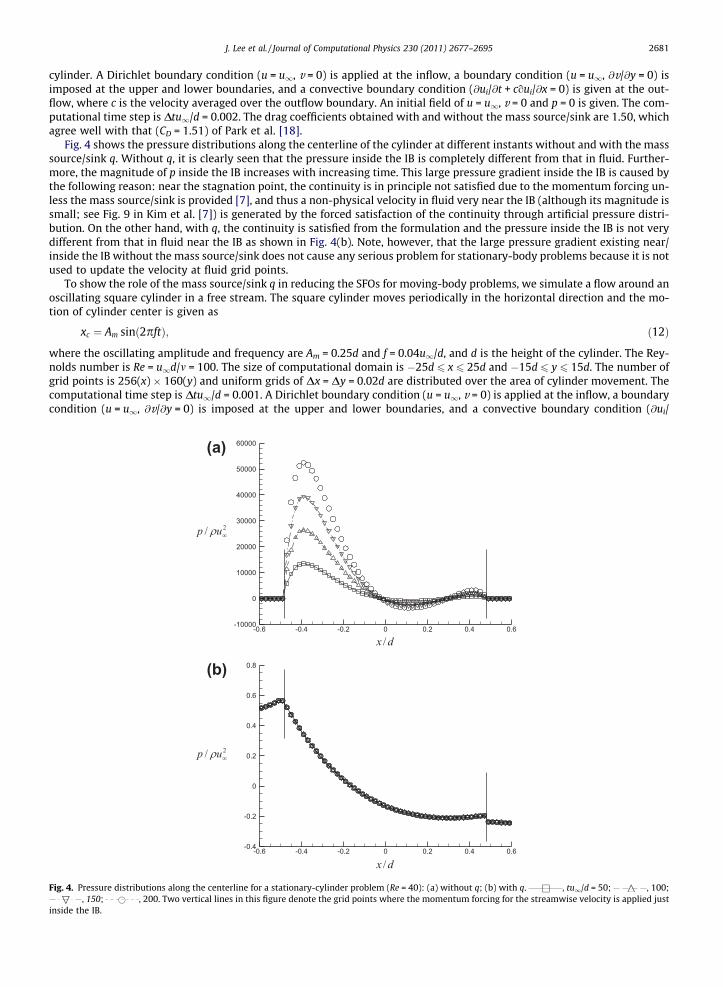
Fig. 4 shows the pressure distributions along the centerline of the cylinder at different instants without and with the masssource/sink q. Without q, it is clearly seen that the pressure inside the IB is completely different from that in fluid. Further-more, the magnitude of p inside the IB increases with increasing time. This large pressure gradient inside the IB is caused bythe following reason: near the stagnation point, the continuity is in principle not satisfied due to the momentum forcing un-less the mass source/sink is provided [7], and thus a non-physical velocity in fluid very near the IB (although its magnitude issmall; see Fig. 9 in Kim et al. [7]) is generated by the forced satisfaction of the continuity through artificial pressure distri-bution. On the other hand, with q, the continuity is satisfied from the formulation and the pressure inside the IB is not verydifferent from that in fluid near the IB as shown in Fig. 4(b). Note, however, that the large pressure gradient existing near/inside the IB without the mass source/sink does not cause any serious problem for stationary-body problems because it is notused to update the velocity at fluid grid points.

To show the role of the mass source/sink q in reducing the SFOs for moving-body problems, we simulate a flow around anoscillating square cylinder in a free stream. The square cylinder moves periodically in the horizontal direction and the mo-tion of cylinder center is given as

Fig. 4.

inside t

xc ¼ Am sinð2pftÞ; ð12Þ

where the oscillating amplitude and frequency are Am = 0.25d and f = 0.04u1/d, and d is the height of the cylinder. The Rey-nolds number is Re = u1d/m = 100. The size of computational domain is �25d 6 x 6 25d and �15d 6 y 6 15d. The number ofgrid points is 256(x) � 160(y) and uniform grids of Dx = Dy = 0.02d are distributed over the area of cylinder movement. Thecomputational time step is Dtu1/d = 0.001. A Dirichlet boundary condition (u = u1, v = 0) is applied at the inflow, a boundarycondition (u = u1, @v/@y = 0) is imposed at the upper and lower boundaries, and a convective boundary condition (@ui/

(a)

(b)

Pressure distributions along the centerline for a stationary-cylinder problem (Re = 40): (a) without q; (b) with q. , tu1/d = 50; , 100;, 150; , 200. Two vertical lines in this figure denote the grid points where the momentum forcing for the streamwise velocity is applied just

he IB.

2682 J. Lee et al. / Journal of Computational Physics 230 (2011) 2677–2695

@t + c@ui/@x = 0) is given at the outflow, where c is the velocity averaged over the outflow boundary. We compute this flow foreight oscillation periods with the mass source/sink q, and then the time is set to be zero (i.e. t = 0). We further simulate theflow with q until tu1/d = 4.2. After this time, two simulations are conducted with and without q, respectively. As depicted inFig. 5, the square cylinder crosses over a grid line during tu1/d = 4.280–4.281.

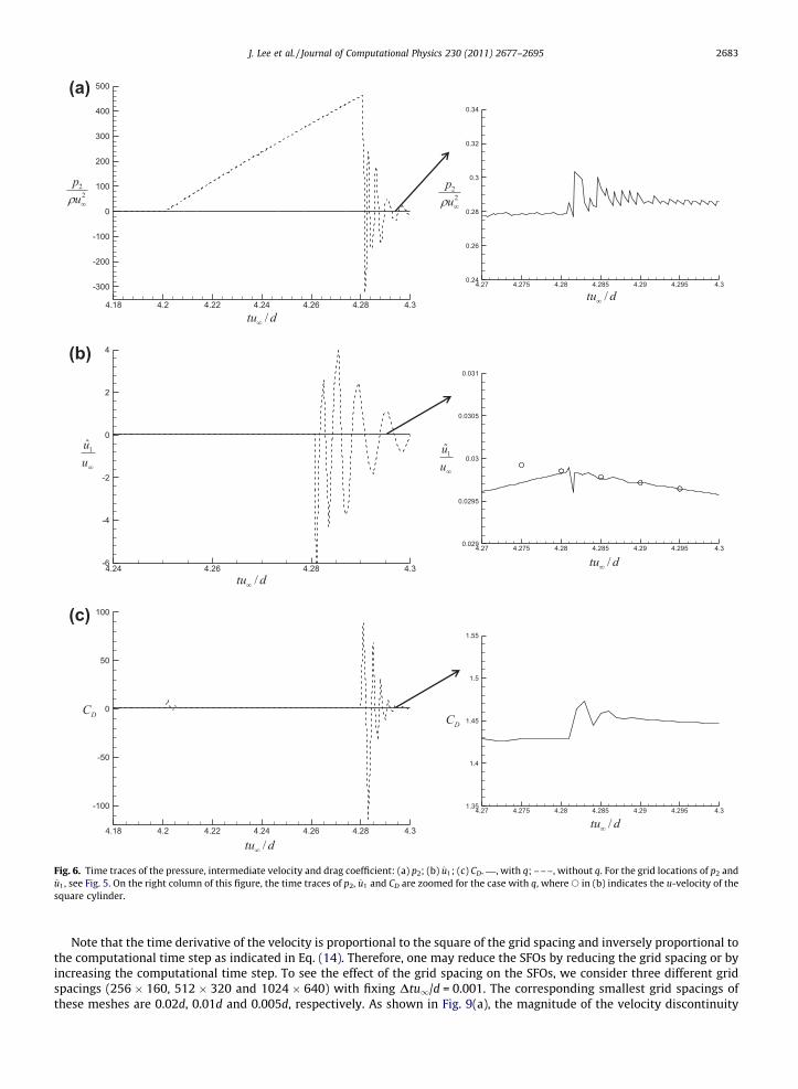
Fig. 6 shows the temporal behaviors of p2, u1 (see Fig. 5 for their grid locations) and CD during tu1/d = 4.2–4.3, where u1 isthe intermediate velocity of u1 from the first step of the fractional step method. Without q, the pressure p2 rapidly increasesbefore the IB passes through the cell face, and shows 2 � Dt wave oscillations thereafter (Fig. 6(a)). Then, the intermediatevelocity u1 (and thus u1) located in fluid is contaminated by this non-physical pressure distribution near the IB (Fig. 6(b)).These contaminations produce the SFOs on the body as seen in Fig. 6(c). On the other hand, with q, much smaller oscillationsare found in the pressure, velocity and body force (see the right column of Fig. 6), showing the role of q in reducing the SFOssignificantly.

3.2. Temporal discontinuity in the velocity

Theoretically, the velocity at the first grid point (ui) outside the IB should approach the solid-body velocity ðUSiÞ as the

distance between the first grid point and IB decreases with the motion of solid body. However, in the framework of the pres-ent IB method (also of other types of IB methods), when the IB approaches very near the first grid point, ui converges to USi

with a second-order spatial discretization error due to the second-order interpolation using local velocities near the IB: i.e.,

Fig. 5.the bot

ui ¼ USiþ O Dx2

j

� ; ð13Þ

where Dxj’s are the grid spacings for the numerical cell containing the IB. Note that Dxj is not the distance between the IB andfirst grid location.

When this grid locates in solid with a body motion at the next time step, its velocity is suddenly changed to satisfy the no-slip condition on the IB through the momentum forcing. Assuming negligibly small acceleration of the solid body for sim-plicity, the time derivative of the velocity at this grid point becomes

@ui

@t¼ 1

DtO Dx2

j

� : ð14Þ

This velocity discontinuity in time subsequently generates non-physical behaviors of the pressure near the IB (@ui/@t � @p/@xi) and the body force (see below).

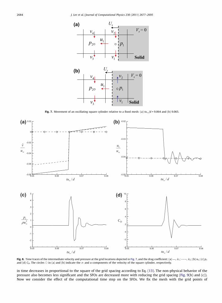
We again consider the oscillating square cylinder in a free stream adopted in the previous sub-section. Fig. 7 shows twosuccessive time instants, respectively, before and after the cylinder surface crosses over the grid points where the transversevelocities, v1 and v2, are defined. Fig. 8(a) shows the temporal behaviors of the intermediate velocities, v1 and v2, at the gridpoints shown in Fig. 7. The transverse locations of these grids are, respectively, 0.1d and 0.12d above the bottom surface ofthe cylinder. As shown in Fig. 8, the velocities (v1; v2;u1) and pressure p1 are abruptly changed when the IB passes throughthese grid points. The drag coefficient also shows a non-physical oscillating behavior.

(a)

(b)

Movement of an oscillating square cylinder relative to a fixed mesh: (a) tu1/d = 4.280; (b) 4.281. Here, the y location for u1, p1 and p2 is 0.11d abovetom surface of the cylinder.

(a)

(b)

(c)

Fig. 6. Time traces of the pressure, intermediate velocity and drag coefficient: (a) p2; (b) u1; (c) CD.3, with q; –––, without q. For the grid locations of p2 andu1, see Fig. 5. On the right column of this figure, the time traces of p2, u1 and CD are zoomed for the case with q, where s in (b) indicates the u-velocity of thesquare cylinder.

J. Lee et al. / Journal of Computational Physics 230 (2011) 2677–2695 2683

Note that the time derivative of the velocity is proportional to the square of the grid spacing and inversely proportional tothe computational time step as indicated in Eq. (14). Therefore, one may reduce the SFOs by reducing the grid spacing or byincreasing the computational time step. To see the effect of the grid spacing on the SFOs, we consider three different gridspacings (256 � 160, 512 � 320 and 1024 � 640) with fixing Dtu1/d = 0.001. The corresponding smallest grid spacings ofthese meshes are 0.02d, 0.01d and 0.005d, respectively. As shown in Fig. 9(a), the magnitude of the velocity discontinuity

(a)

(b)

Fig. 7. Movement of an oscillating square cylinder relative to a fixed mesh: (a) tu1/d = 9.064 and (b) 9.065.

(a)

(c)

(b)

(d)

Fig. 8. Time traces of the intermediate velocity and pressure at the grid locations depicted in Fig. 7, and the drag coefficient: (a)3, v1; –––, v2; (b) u1; (c) p1

and (d) CD. The circles s in (a) and (b) indicate the v- and u-components of the velocity of the square cylinder, respectively.

2684 J. Lee et al. / Journal of Computational Physics 230 (2011) 2677–2695

in time decreases in proportional to the square of the grid spacing according to Eq. (13). The non-physical behavior of thepressure also becomes less significant and the SFOs are decreased more with reducing the grid spacing (Fig. 9(b) and (c)).Now we consider the effect of the computational time step on the SFOs. We fix the mesh with the grid points of

(a)

(b)

(c)

Fig. 9. Variations of the temporal behaviors of the velocity, pressure and drag coefficient with the grid spacing by fixing Dtu1/d = 0.001: (a) v1; (b) p1; (c)CD. 3, Dxmin = Dymin = 0.02d; –––, 0.01d; –�–�–, 0.005d.

J. Lee et al. / Journal of Computational Physics 230 (2011) 2677–2695 2685

256 � 160 and vary the computational time step: Dtu1/d = 0.001, 0.002 and 0.004. As shown in Fig. 10, the magnitudes of thevelocity jump are nearly the same regardless of the size of the computational time step, which results in smaller @ui/@t forlarger Dt. Accordingly, the pressure oscillations and SFOs decrease with increasing the computational time step.

3.3. Combined effect of the grid spacing and the computational time step size

As indicated by Eq. (14), the SFOs are suppressed with smaller grid spacing and larger computational time step size. Whena numerical simulation is performed, a constant Dt or a constant CFL number is used. In the latter case, Dt becomes smallerwith smaller grid spacing. Thus, it is interesting to see how the SFOs are changed due to the combined effect of Dt and Dxi

when a constant CFL number is chosen during the simulation.

(a) (b)

(d)(c)

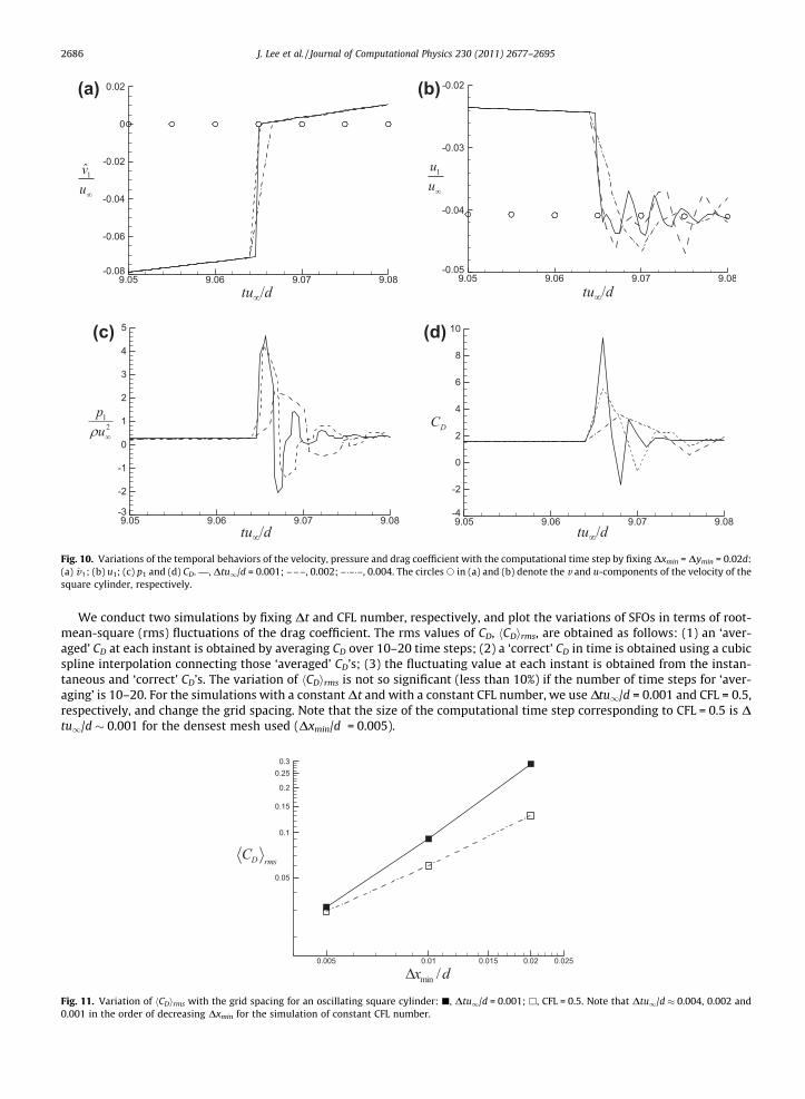
Fig. 10. Variations of the temporal behaviors of the velocity, pressure and drag coefficient with the computational time step by fixing Dxmin = Dymin = 0.02d:(a) v1; (b) u1; (c) p1 and (d) CD.3, Dtu1/d = 0.001; –––, 0.002; –�–�–, 0.004. The circles s in (a) and (b) denote the v and u-components of the velocity of thesquare cylinder, respectively.

2686 J. Lee et al. / Journal of Computational Physics 230 (2011) 2677–2695

We conduct two simulations by fixing Dt and CFL number, respectively, and plot the variations of SFOs in terms of root-mean-square (rms) fluctuations of the drag coefficient. The rms values of CD, hCDirms, are obtained as follows: (1) an ‘aver-aged’ CD at each instant is obtained by averaging CD over 10–20 time steps; (2) a ‘correct’ CD in time is obtained using a cubicspline interpolation connecting those ‘averaged’ CD’s; (3) the fluctuating value at each instant is obtained from the instan-taneous and ‘correct’ CD’s. The variation of hCDirms is not so significant (less than 10%) if the number of time steps for ‘aver-aging’ is 10–20. For the simulations with a constant Dt and with a constant CFL number, we use Dtu1/d = 0.001 and CFL = 0.5,respectively, and change the grid spacing. Note that the size of the computational time step corresponding to CFL = 0.5 is Dtu1/d � 0.001 for the densest mesh used (Dxmin/d = 0.005).

Fig. 11. Variation of hCDirms with the grid spacing for an oscillating square cylinder: j, Dtu1/d = 0.001; h, CFL = 0.5. Note that Dtu1/d � 0.004, 0.002 and0.001 in the order of decreasing Dxmin for the simulation of constant CFL number.

J. Lee et al. / Journal of Computational Physics 230 (2011) 2677–2695 2687

Fig. 11 shows the variation of hCDirms with the grid spacing. The hCDirms decreases with reducing the grid spacing for bothcases of constant Dt and CFL number. The decreasing rate of hCDirms with reducing Dx is bigger for the case of constant Dtthan for the case of constant CFL number. For the case of constant CFL number, Dt decreases with decreasing Dx. As shownbefore, decreasing Dx reduces hCDirms but decreasing Dt increases it. However, the combined effect is the reduction of hCDirms

for the case of constant CFL number. This indicates that the role of the grid spacing is more important in reducing the SFOsthan that of the computational time step size. Note that, for the coarsest mesh, the simulation with Dtu1/d = 0.001 results in

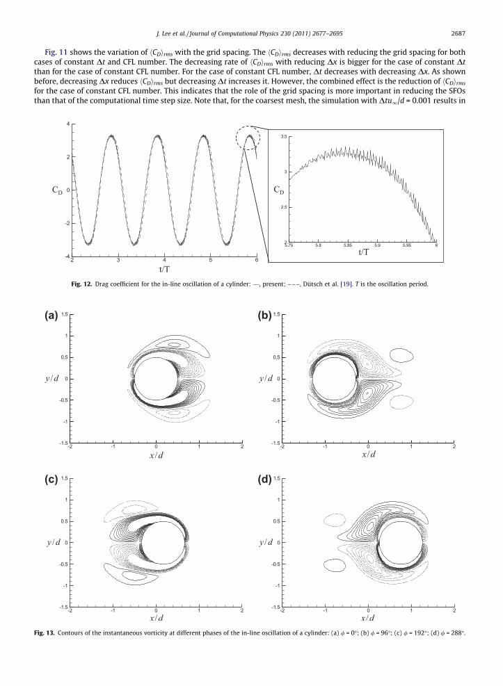
Fig. 12. Drag coefficient for the in-line oscillation of a cylinder: 3, present; –––, Dütsch et al. [19]. T is the oscillation period.

(a)

(c) (d)

(b)

Fig. 13. Contours of the instantaneous vorticity at different phases of the in-line oscillation of a cylinder: (a) / = 0�; (b) / = 96�; (c) / = 192�; (d) / = 288�.

2688 J. Lee et al. / Journal of Computational Physics 230 (2011) 2677–2695

a bigger hCDirms than that with CFL = 0.5 because Dtu1/d of the latter case is about 0.004. For the case of constant Dt, theslope of hCDirms is approximately O(Dx2), whereas it is O(Dx) for the case of constant CFL number, which agrees withO(Dx2)/Dt in Eq. (14) because Dt � Dx for the case of constant CFL number.

So far, the flow around an oscillating square cylinder has been considered in this section. The body forces were obtainedby the method described in Section 2.2 (Eq. (11)), i.e. integrating the momentum forcing fi and another term rather than di-rectly integrating the surface pressure and skin friction. In the latter case, it should be interesting to see if these surface vari-ables show spatial oscillations in addition to temporal ones. For the present square cylinder problem, the immersedboundary passes through all the nearest grid points on its left or right side within one time step. Thus, spatial oscillationsof surface pressure are not much expected and only temporal oscillations are expected. In Section 4.2, we will show spatialand temporal distributions of surface pressure for the case of circular cylinder, in which the immersed boundary alwayspasses through some grid points in the domain with its movement in time.

4. More numerical examples

In this section, three more flow problems are considered and the results are presented.

4.1. In-line oscillation

The flow induced by an in-line oscillation of a circular cylinder in a fluid at rest [19] is simulated. The cylinder oscillatesharmonically in the horizontal direction (x) and its motion is described as

xcðtÞ ¼ �Am sinð2pftÞ; ð15Þ

where xc is the streamwise location of the cylinder center, and Am and f are the amplitude and frequency of the cylinder mo-tion, respectively. The flow characteristics is determined by two key parameters: the Reynolds and Keulegan–Carpenter

Fig. 14. Drag coefficients for the in-line oscillation of a cylinder (Dtum/d = 0.005): - -- ---, Dxmin = Dymin = 0.04d; 3, Dxmin = Dymin = 0.01d.

Fig. 15. Variation of hCDirms with the grid spacing for the in-line oscillation of a cylinder: j, Dtum/d = 0.005; h, CFL = 0.5.

J. Lee et al. / Journal of Computational Physics 230 (2011) 2677–2695 2689

numbers. These numbers are defined as Re = umd/m and KC = um/(fd), where um is the maximum velocity of the oscillating cyl-inder, d is the cylinder diameter and m is the kinematic viscosity.

We consider Re = 100 and KC = 5 following Dütsch et al. [19]. The domain size is 50d � 30d and the number of grid pointsis 310 � 160 in x and y directions, respectively. The grids are uniformly distributed (Dx = Dy = 0.02d) in the region where thecylinder oscillates and then stretched outside. The computational time step is Dt = 0.005d/um and the Dirichlet boundarycondition (ui = 0) is applied to all outer boundaries. Fig. 12 shows the time trace of drag coefficient from the present study,together with that of Dütsch et al. [19]. As shown, the present result agrees very well with that of Dütsch et al. [19], but itcontains the SFOs with the mesh used. Fig. 13 shows the contours of the instantaneous vorticity around the cylinder at four

Fig. 16. Time traces of the drag coefficient for a cross-flow oscillating cylinder at fe/f0 = 1.0: ---- ---, Dxmin = Dymin = 0.04d; 3, Dxmin = Dymin = 0.01d.

(a)

(b)

Fig. 17. Pressure distributions along the cylinder surface at consecutive time steps for a cross-flow oscillating cylinder (fe/f0 = 1.0 and Dtu1/d = 0.005): (a) Dxmin = Dymin = 0.04d; (b) Dxmin = Dymin = 0.01d. , tu1/d = 112.170; , 112.175; ,112.180; , 112.185.

2690 J. Lee et al. / Journal of Computational Physics 230 (2011) 2677–2695

different phases. The vorticity contours are smooth even near the cylinder surface irrespective of the existence of the high-frequency SFOs shown in Fig. 12.

We use three other meshes and their grid points are 156 � 80, 248 � 128, and 620 � 320, having smallest grid spacings of0.04d, 0.025d and 0.01d, respectively. Two different simulations are conducted with a constant time step of Dtum/d = 0.005and with a constant CFL number of 0.5, respectively. As seen in Fig. 14, the drag coefficient has large SFOs for the mesh of156 � 80 but has nearly no SFOs for the mesh of 620 � 320.

Fig. 15 shows the variation of hCDirms with the grid spacing for both cases of constant Dtum/d of 0.005 and constant CFLnumber of 0.5. Here, the computational time step corresponding to CFL = 0.5 for the densest mesh is Dtum/d � 0.005. TheSFOs are reduced with decreasing the grid spacing for both cases, and they decrease more rapidly with constant Dt than withconstant CFL number, supporting the result in the previous section.

4.2. Cross-flow oscillation

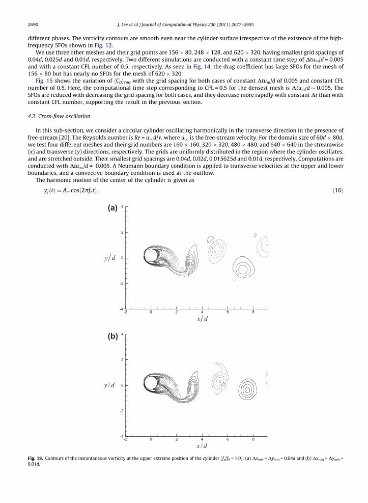
In this sub-section, we consider a circular cylinder oscillating harmonically in the transverse direction in the presence offree-stream [20]. The Reynolds number is Re = u1d/m, where u1 is the free-stream velocity. For the domain size of 60d � 80d,we test four different meshes and their grid numbers are 160 � 160, 320 � 320, 480 � 480, and 640 � 640 in the streamwise(x) and transverse (y) directions, respectively. The grids are uniformly distributed in the region where the cylinder oscillates,and are stretched outside. Their smallest grid spacings are 0.04d, 0.02d, 0.015625d and 0.01d, respectively. Computations areconducted with Dtu1/d = 0.005. A Neumann boundary condition is applied to transverse velocities at the upper and lowerboundaries, and a convective boundary condition is used at the outflow.

The harmonic motion of the center of the cylinder is given as

Fig. 18.0.01d.

ycðtÞ ¼ Am cosð2pfetÞ; ð16Þ

(a)

(b)

Contours of the instantaneous vorticity at the upper extreme position of the cylinder (fe/f0 = 1.0): (a) Dxmin = Dymin = 0.04d and (b) Dxmin = Dymin =

J. Lee et al. / Journal of Computational Physics 230 (2011) 2677–2695 2691

where Am and fe are the amplitude and frequency of the oscillatory motion. The Reynolds number is 185 and the range ofoscillation frequency is 0.8 6 fe/f0 6 1.2, following Guilmineau and Queuty [20]. Here, f0(=0.193u1/d) is the natural sheddingfrequency for the stationary cylinder. The mean drag, and rms drag and lift fluctuations obtained from the densest gridsagree well with those from Guilmineau and Queuty [20], although the mean drag coefficient is slightly higher from the pres-ent study like the result by Yang and Balaras [13].

(a)

(b)

Fig. 19. Variations of hCDirms and hCLirms with the grid spacing for a cross-flow oscillating cylinder (fe/f0 = 1.0): (a) hCDirms; (b) hCLirms. j, Dtum/d = 0.005; h,CFL = 1.0.

Fig. 20. Schematic diagram of a wing flapping motion [21,22]. Here FV and FH denote the vertical and horizontal forces on the wing.

2692 J. Lee et al. / Journal of Computational Physics 230 (2011) 2677–2695

Fig. 16 shows the time traces of the drag coefficient for the cases of coarsest and densest meshes used. As shown, thecoarsest mesh produces large SFOs, whereas the densest mesh has very small SFOs. In Fig. 17, we show the pressure distri-butions along the cylinder surface at three consecutive time steps for the coarse and dense meshes. Because of the geometryof the circular cylinder, the immersed boundary always passes through some grid points with its movement in time andthus we may expect spatial oscillations of pressure and skin-friction along the cylinder surface. As shown in Fig. 17(a), whenthe resolution is not dense enough, there are significant pressure oscillations along the cylinder surface as well as in time.However, those oscillations nearly disappear with dense grid resolution (Fig. 17(b)). The skin-friction distribution alsoshowed a similar behavior although its oscillations were much smaller than those of surface pressure (not shown in thispaper).

Fig. 18 shows the contours of the instantaneous vorticity at the upper extreme position of the cylinder for the cases ofcoarsest and densest meshes. Although the SFOs are large for the case of coarsest mesh, the contours of vorticity are not verydifferent even near the cylinder surface as compared to those of densest mesh. Fig. 19 shows the variations of hCDirms andhCLirms with the grid spacing for both cases of constant computational time step of Dtu1/d = 0.005 and constant CFL numberof 1.0. Here, the computational time step corresponding to CFL = 1.0 for the densest mesh is Dtu1/d � 0.005. As the previousexamples, the SFOs are reduced with decreasing the grid spacing for both cases, and they decrease more rapidly with con-stant Dt than with constant CFL number.

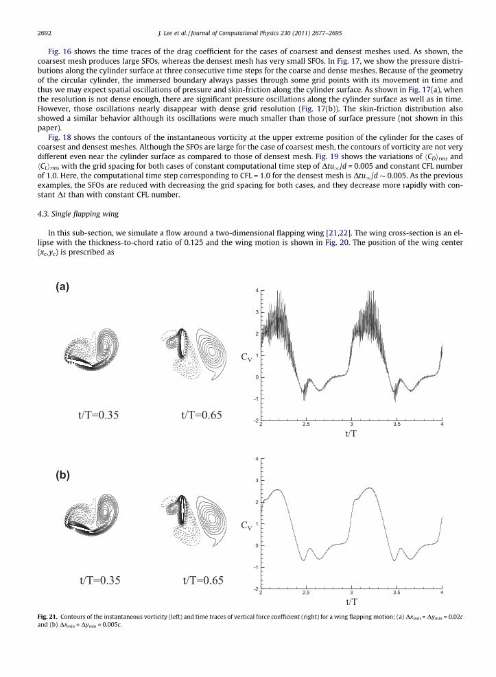
4.3. Single flapping wing

In this sub-section, we simulate a flow around a two-dimensional flapping wing [21,22]. The wing cross-section is an el-lipse with the thickness-to-chord ratio of 0.125 and the wing motion is shown in Fig. 20. The position of the wing center(xc,yc) is prescribed as

(a)

(b)

Fig. 21. Contours of the instantaneous vorticity (left) and time traces of vertical force coefficient (right) for a wing flapping motion: (a) Dxmin = Dymin = 0.02cand (b) Dxmin = Dymin = 0.005c.

Fig. 2

J. Lee et al. / Journal of Computational Physics 230 (2011) 2677–2695 2693

xc ¼ 0:5Am cosð2pftÞ cos b;

yc ¼ 0:5Am cosð2pftÞ sin b;ð17Þ

where Am is the stroke amplitude, f is the wing beat frequency and b is the angle of the stroke plane to the horizontal axis asshown in Fig. 20. The angle a in Fig. 20 is the angle between the chord axis and the stroke plane. The wing rotates counter-clockwise and clockwise at the ends of upstroke and downstroke, respectively. These rotations are called pronation and supi-nation, respectively, and a is prescribed for modeling the rotations as follows [22]:

aðtÞ ¼5

24 p tanhð�2tÞ þ 58 p for � T

4 6 t < T4 ;

524 p tanh 2 t � T

2

� � �þ 5

8 p otherwise;

(ð18Þ

where T is the period of the wing flapping. The Reynolds number is defined as Re = umc/m based on the maximum transla-tional velocity um and the chord length c. We choose one case among those simulated by Kim and Choi [22], where theparameters are determined as Re = 150, Am = 2.5c and b = 60�. The computational domain is �10c 6 x 6 10c and �10c 6 y 610c, and a Dirichlet boundary condition (ui = 0) is used for all outer boundaries.

We consider four different mesh sizes. The numbers of the grid points are 192 � 224, 220 � 256, 410 � 464 and780 � 864 and their smallest grid spacings are 0.025c, 0.02c, 0.01c and 0.005c, respectively. The computational time stepis set to be Dtum/c = 0.004 for the case of constant time step or to be adjusted to satisfy constant CFL number of 1.0. Uniformgrids with smallest grid spacing are distributed on and near the path of the wing flapping motion.

Fig. 21 shows the contours of the instantaneous vorticity around the flapping wing at two different instants (t/T = 0.35 and0.65) and the time traces of vertical force coefficient on the wing for the cases of coarse and densest meshes. The coarse meshproduces large SFOs, but the densest one has nearly no SFOs. The vorticity contours are almost identical to each other for alldifferent meshes. The variations of rms SFOs with the grid spacing are shown in Fig. 22. The SFOs are reduced as the gridspacing decreases, and the case with constant time step produces more rapid decrease than the case with constant CFL num-ber. The decrease of SFOs with decreasing grid spacing even for the case of constant CFL number confirms that the effect ofgrid spacing is more dominant in reducing the SFOs than that of computational time step size.

(a)

(b)

2. Variations of hCHirms and hCVirms with the grid spacing for a wing flapping motion: (a) hCHirms and (b) hCVirms. j, Dtum/c = 0.004; h, CFL = 1.0.

2694 J. Lee et al. / Journal of Computational Physics 230 (2011) 2677–2695

In this flow, we needed to locate minimum three grid points inside the flapping wing to avoid spurious pressure oscilla-tions across the body owing to the differences in the pressures at both wing surfaces. A similar grid-point requirementshould be necessary for other types of thin-body flow problems, although the minimum number of grid points inside thinsolid body should depend on its geometry and the Reynolds number. In our IB method [7], we require grid points insidethe solid body for the interpolation purpose, and thus we may not be able to handle an infinitesimally thin body with currentIB method if that kind of geometry is physically required. However, other types of IB methods that do not require grid pointsinside a body (e.g. that of [6]) may not be either successful in eliminating SFOs because of the discontinuity in the pressureacross the body. Uhlmann [12] and Vanella and Balaras [23] used transfer functions to obtain the momentum forcing at theEulerian grids from the forcing calculated on the Lagrangian points of a solid body. This type of IB methods may result insmaller discontinuity in the pressure across the IB due to smooth distribution of momentum forcing on the Eulerian grids.

5. Conclusions

In the present study, we identified two main sources of spurious force oscillations (SFOs) occurred when a discrete-forc-ing IB method is used for simulation of moving-body problems in an inertial coordinate. One source is the pressure discon-tinuity across the IB when the grid point locates in fluid from in solid. Due to the momentum forcing on or inside the IB, thepressure there has a discontinuity across the IB. In the next time step, the grid point locates in fluid from in solid and has anon-physical pressure gradient, which contaminates the velocity at that grid point and produces the SFOs. It was shown inthe present study that the mass source/sink suggested by Kim et al. [7] is effective in reducing the SFOs.

The other source is the temporal discontinuity in the velocity near the IB. When the grid point locates in solid from influid, the velocity there is considerably changed from the value at the previous time step because the momentum forcingis newly imposed on the grid point due to the body motion. This sudden velocity change induces an abrupt pressure changeand pressure oscillations, resulting in the SFOs.

In the present study, we showed that the SFOs are reduced with reducing the grid spacing, but they are increased withreducing the computational time step size (at fixed grid spacing). Four moving-body problems (a moving square cylinder, in-line oscillation and cross-flow oscillation of a cylinder, and single flapping wing) were simulated to investigate which of thetwo factors (i.e. grid spacing and computational time step size) is more dominant. With decreasing the grid spacing for eachproblem, we fix the computational time step or the CFL number. In the latter case, the computational time step size de-creases as the grid spacing is reduced. It was shown that for both cases the SFOs are reduced with decreasing the grid spac-ing, but they are more rapidly reduced for the case of constant computational time step than that of constant CFL number.This indicates that the grid spacing is the dominant factor in reducing the SFOs.

Acknowledgments

This work was supported by the National Research Laboratory Program of Ministry of Education, Science and Technology,Korea (R0A-2006-000-10180-0). This work was also partly supported by the WCU Program (R31-2008-000-10083-0).

References

[1] C.S. Peskin, Flow patterns around heart valves: a numerical method, Journal of Computational Physics 10 (1972) 252–271.[2] C.S. Peskin, Numerical analysis of blood flow in the heart, Journal of Computational Physics 25 (1977) 220–252.[3] D. Goldstein, R. Handler, L. Sirovich, Modeling a no-slip flow boundary with an external force field, Journal of Computational Physics 105 (1993) 354–

366.[4] J. Mohd-Yusof, Combined immersed-boundary/B-spline methods for simulations of flow in complex geometries, Annual Research Briefs (Center for

Turbulence Research, NASA Ames and Stanford University), 1997, pp. 317–327.[5] M. Lai, C.S. Peskin, An immersed boundary method with formal second-order accuracy and reduced numerical viscosity, Journal of Computational

Physics 160 (2000) 705–719.[6] E.A. Fadlun, R. Verzicco, P. Orlandi, J. Mohd-Yusof, Combined immersed-boundary finite-difference methods for three-dimensional complex flow

simulations, Journal of Computational Physics 161 (2000) 35–60.[7] J. Kim, D. Kim, H. Choi, An immersed-boundary finite volume method for simulations of flow in complex geometries, Journal of Computational Physics

171 (2001) 132–150.[8] Z. Li, M. Lai, The immersed interface method for the Navier–Stokes equations with singular forces, Journal of Computational Physics 171 (2001) 822–

842.[9] C. Peskin, The immersed boundary method, Acta Numerica 11 (2002) 1–39.

[10] Y. Tseng, J.H. Ferziger, A ghost-cell immersed boundary method for flow in complex geometry, Journal of Computational Physics 192 (2003) 593–623.[11] E. Balaras, Modeling complex boundaries using an external force field on fixed Cartesian grids in large-eddy simulations, Computers and Fluids 33

(2004) 375–404.[12] M. Uhlmann, An immersed boundary method with direct forcing for the simulation of particulate flows, Journal of Computational Physics 209 (2005)

448–476.[13] J. Yang, E. Balaras, An embedded-boundary formulation for large-eddy simulation of turbulent flows interacting with moving boundaries, Journal of

Computational Physics 215 (2006) 12–40.[14] K. Taira, T. Colonius, The immersed boundary method: a projection approach, Journal of Computational Physics 225 (2007) 2118–2137.[15] S. Kang, G. Iaccarino, P. Moin, Accurate immersed-boundary reconstructions for viscous flow simulations, AIAA Journal 47 (2009) 1750–1760.[16] R. Mittal, G. Iaccarino, Immersed boundary methods, Annual Review of Fluid Mechanics 37 (2005) 239–261.[17] D. Kim, H. Choi, Immersed boundary method for flow around an arbitrarily moving body, Journal of Computational Physics 212 (2006) 662–680.[18] J. Park, K. Kwon, H. Choi, Numerical solutions of flow past a circular cylinder at Reynolds numbers up to 160, KSME International Journal 12 (6) (1998)

1200–1205.

J. Lee et al. / Journal of Computational Physics 230 (2011) 2677–2695 2695

[19] H. Dütsch, F. Durst, S. Becker, H. Lienhart, Low-Reynolds-number flow around an oscillating circular cylinder at low Keulegan–Carpenter numbers,Journal of Fluid Mechanics 360 (1998) 249–271.

[20] E. Guilmineau, P. Queutey, A numerical simulation of vortex shedding from an oscillating circular cylinder, Journal of Fluids and Structures 16 (6)(2002) 773–794.

[21] J. Wang, Two dimensional mechanism for insect hovering, Physical Review Letter 85 (10) (2000) 2216–2219.[22] D. Kim, H. Choi, Two-dimensional mechanism of hovering flight by single flapping wing, Journal of Mechanical Science and Technology 21 (1) (2007)

207–221.[23] M. Vanella, E. Balaras, A moving-least-squares reconstruction for embedded-boundary formulations, Journal of Computational Physics 228 (2009)

6617–6628.