Forschungsinstitut zur Zukunft der ArbeitInstitute for the Study of Labor

DI

SC

US

SI

ON

P

AP

ER

S

ER

IE

S

Sorting around the Discontinuity Threshold:The Case of a Neighbourhood Investment Programme

IZA DP No. 9838

March 2016

Sander GerritsenDinand WebbinkBas ter Weel

Sorting around the Discontinuity Threshold: The Case of a Neighbourhood

Investment Programme

Sander Gerritsen CPB Netherlands Bureau for Economic Policy Analysis

Dinand Webbink

Erasmus University Rotterdam and IZA

Bas ter Weel

CPB Netherlands Bureau for Economic Policy Analysis, Maastricht University and IZA

Discussion Paper No. 9838 March 2016

IZA

P.O. Box 7240 53072 Bonn

Germany

Phone: +49-228-3894-0 Fax: +49-228-3894-180

E-mail: iza@iza.org

Any opinions expressed here are those of the author(s) and not those of IZA. Research published in this series may include views on policy, but the institute itself takes no institutional policy positions. The IZA research network is committed to the IZA Guiding Principles of Research Integrity. The Institute for the Study of Labor (IZA) in Bonn is a local and virtual international research center and a place of communication between science, politics and business. IZA is an independent nonprofit organization supported by Deutsche Post Foundation. The center is associated with the University of Bonn and offers a stimulating research environment through its international network, workshops and conferences, data service, project support, research visits and doctoral program. IZA engages in (i) original and internationally competitive research in all fields of labor economics, (ii) development of policy concepts, and (iii) dissemination of research results and concepts to the interested public. IZA Discussion Papers often represent preliminary work and are circulated to encourage discussion. Citation of such a paper should account for its provisional character. A revised version may be available directly from the author.

IZA Discussion Paper No. 9838 March 2016

ABSTRACT

Sorting around the Discontinuity Threshold: The Case of a Neighbourhood Investment Programme*

This paper investigates the empirical validity of the setup of a large-scale government neighbourhood investment programme in the Netherlands. Selection of neighbourhoods into the programme was determined by their score on a predetermined index. At first sight this is a textbook example for the application of a regression discontinuity (RD) design to estimate the causal effect of the programme on neighbourhood outcomes. However, at the discontinuity threshold we find a large gap in the share of non-Western immigrants. In addition, the pattern of non-compliance with the assignment rule is consistent with investing in neighbourhoods with a high share of non-Western immigrants. Finally, the way of selecting neighbourhoods into the programme could be a likely explanation for the imbalance at the discontinuity threshold. This case illustrates that RD designs can become invalid even when treatment and control groups have no influence on the assignment. JEL Classification: C90, D70, R58 Keywords: regression discontinuity designs, government decision-making processes,

neighbourhood investment programmes Corresponding author: Bas ter Weel CPB Board of Directors PO Box 80510 2508 GM Den Haag The Netherlands E-mail: b.ter.weel@cpb.nl

* We thank Josh Angrist, Casper van Ewijk, Erzo Luttmer, Justin McCrary, Coen Teulings and participants at several seminars for helpful comments and discussions. We also benefited useful discussions about the neighbourhood programme with representatives from the Dutch Ministry of the Interior and Kingdom Relations and the Dutch Ministry of Ministry of Health, Welfare and Sports. Special thanks to Gerard Verweij for constructing the graphs in this paper. We would like to thank Joost Smits for access to the election data.

IZA Discussion Paper No. 9838 March 2016

NON-TECHNICAL SUMMARY

In the Netherlands, a neighbourhood investment programme was implemented in 2008. It consisted of large scale neighbourhood investments in social and physical infrastructure aimed at improving the living conditions in 40 disadvantaged neighbourhoods (Vogelaarwijken). In the period 2008-2011 the Dutch government invested 216 million Euros, while an additional amount of one billion Euros was invested by housing corporations. Such investment programmes have been evaluated using several different econometric techniques. A popular way to estimate treatment effects is by making use of regression discontinuity (RD) designs. One of the main reasons for this is that variation around the cut-off value, which determines assignment to the treatment, can be considered as good as random. The reason for this is that those who take part in the programme have no control over the assignment. However, knowledge about the assignment rule might influence the assignment to the treatment and thereby invalidate the key assumption that individuals on either side of the discontinuity threshold are similar. This research documents a case of sorting disadvantaged areas into the neighbourhood investment programme. Policymakers at the national level, who designed and implemented the assignment rules for the policy in disadvantaged neighbourhoods, sorted areas into and out of the programme in such a way that there exists a large discontinuity in the share of non-Western immigrants at the discontinuity threshold. At the threshold value for the assignment to the treatment we find a large and statistically significant gap in the proportion of non-Western immigrants of between 11 and 21 percentage points. Moreover, there exists non-compliance with a bias toward removing areas with lower shares of non-Western immigrants from the treatment group. The violation of a continuous distribution around the discontinuity threshold of this important characteristic could be due to the way the selection process of neighbourhoods has been carried out. Politicians at the national level demanded that there had to be a list of 40 eligible neighbourhoods. To determine the 40 neighbourhoods, a two-step procedure has been used. In the first step, a preliminary list of 40 neighbourhoods was created based on the most disadvantaged postal code areas (PCAs) according to the ‘quality’ index. Because most neighbourhoods consist of multiple adjacent PCAs, policymakers sometimes merged PCAs with different rank numbers to create a neighbourhood. This opens possibilities of adding lower-ranked PCAs to an already identified neighbourhood. When we move down the list of PCAs, it is possible to add more PCAs beyond the point at which 40 geographical areas have been identified as neighbourhoods. This process continues until a PCA from a different geographical area is next on the list and would become neighbourhood number 41. We show that neighbourhood 41 is indeed in another city. In the second step, a number of PCAs were removed from and added to this list to obtain a final list of 40 eligible neighbourhoods. We show that the added neighbourhoods are not close to the discontinuity threshold. We illustrate the bias of the RD estimates when using the official cut-off. We find that the estimates from RD models that do not take account of the endogenous sorting differ from the estimates from RD models that do account for the endogenous sorting. We also show that a different selection process of 40 neighbourhoods does not lead to a discontinuity in the share of non-Western immigrants. Finally, we cannot rule out that the result of selecting 40 neighbourhoods in this way is a case of bad luck. Using the same procedure to select 30 neighbourhoods does not yield the same discontinuities.

1  

1. Introduction

Neighbourhood investment programmes target government transfers toward particular

geographic areas rather than individuals (e.g., Glaeser and Gottlieb, 2008). These investment

programmes have been evaluated using several different econometric techniques. A series of

recent studies in this area have used regression discontinuity (RD) designs to estimate

treatment effects. For example, Busso et al. (2013) evaluate the employment effects of the

U.S. federal urban Empowerment Zone programme; Freedman (2015) studies the labour-

market effects of the New Markets Tax Credit programme in the United States; and Horn

(2015) investigates the relationship between school quality and capital investments in the

housing stock using a boundary discontinuity identification strategy.

RD designs are increasingly used by economists.1 One of the main reasons for this is that

variation around the cut-off value, which determines assignment to the treatment, can be

considered as good as random because those who take part in the programme have no control

over the assignment (e.g., Lee, 2008). This inability to control or influence the assignment to

the treatment suggests that the identifying assumptions required for a valid design are

relatively weak (e.g., Hahn et al., 2001). However, public knowledge about the assignment

rule might influence the assignment to the treatment and thereby invalidate the key

assumption that individuals on either side of the discontinuity threshold are similar. Recent

studies have considered the possibility of such “endogenous sorting” around the discontinuity

threshold and have developed tools to examine its presence and consequences (e.g., Lee, 2008

and McCrary, 2008). In addition, a number of studies offer examples of sorting around the

discontinuity threshold. It seems to be the case that sorting is driven by incentives for

potential receivers of the treatment to select themselves into the treatment, such as home

owners, parents/schools, tax payers or traders on financial markets (e.g., Bayer et al., 2007,

Urquiola and Verhoogen, 2009, Saez, 2010, Bubb and Kaufman, 2014 and Vogl, 2014).

This research adds a novel case to this relatively new literature about cautiousness with

respect to applying RD designs when there are opportunities for influencing the discontinuity

threshold by documenting a case of sorting disadvantaged areas into a large scale

neighbourhood investment programme. The unique feature of our research is that sorting into

the treatment group was impossible for units that were entitled to receiving the treatment.

                                                            1 See Imbens and Lemieux (2008), Angrist and Pischke (2009 and 2010) and Lee and Lemieux (2010) for recent reviews of the application of RD designs in the economic literature and related scientific areas.

2  

Policymakers at the national level, who designed and implemented the assignment rules for

the policy in disadvantaged neighbourhoods, sorted areas into and out of the programme in

such a way that there exists a large discontinuity in the share of non-Western immigrants at

the discontinuity threshold.

The neighbourhood investment programme was implemented in 2008 and consisted of large

scale neighbourhood investments in social and physical infrastructure aimed at improving the

living conditions in disadvantaged neighbourhoods in the Netherlands. Approximately 4,000

postal code areas (PCAs)2 were ranked based on a ‘quality’ index, which was constructed by

making use of eighteen different items. PCAs with the worst outcomes on the index were

selected into the programme and received additional funds. In the end, 83 PCAs received

funding from the programme. Together these 83 PCAs are put together to form 40

neighbourhoods. In the period 2008-2011 the Dutch government invested 216 million Euros

in these 40 neighbourhoods, while an additional amount of one billion Euros was invested by

housing corporations.

The assignment of PCAs to the programme based on the ‘quality’ index score is a textbook

example for the application of a RD design for estimating the causal effect of the programme.

However, at the threshold value for the assignment to the treatment we find a large and

statistically significant gap in the proportion of non-Western immigrants of between 11 and

21 percentage points depending on the specification. Moreover, there is non-compliance

because twelve eligible PCAs have been excluded from the programme, whereas two others

have been added to the treatment group. The observed pattern of non-compliance with the

assignment rule shows a similar difference in the share of non-Western immigrants. These

differences cannot be explained by endogenous sorting induced by local authorities, as they

had no control over the assignment to the treatment. It also seems unlikely that a random

threshold produces such large differences in the proportion of non-Western immigrants at the

discontinuity threshold.

The violation of a continuous distribution around the discontinuity threshold of such an

important baseline characteristic could be due to the way the selection process of

neighbourhoods has been carried out. Politicians at the national level demanded that there had

to be a list of 40 eligible neighbourhoods. To determine the 40 neighbourhoods, a two-step

procedure has been used. In the first step, a preliminary list of 40 neighbourhoods was created

                                                            2 The postal code area is at the four digit level. For instance 1061 in Amsterdam.

3  

based on the most disadvantaged PCAs according to the PCA ‘quality’ index. Because

neighbourhoods can consist of multiple adjacent PCAs, policymakers sometimes merged

PCAs with different rank numbers to create a neighbourhood. This opens possibilities of

adding lower-ranked PCAs to an already identified neighbourhood. When we move down the

list of PCAs, it is possible to add more PCAs beyond the point at which 40 geographical areas

have been identified as neighbourhoods. This process continues until a PCA from a different

geographical area is next on the list and would become neighbourhood number 41. We show

that neighbourhood 41 is indeed in another city. In the second step, a number of PCAs were

removed from and added to this list to obtain a final list of 40 eligible neighbourhoods. The

added neighbourhoods are not close to the discontinuity threshold as we will show below.

We illustrate the bias of the RD estimates when using the official cut-off. We find that the

estimates from RD models that do not take account of the endogenous sorting differ from the

estimates from RD models that do account for the endogenous sorting. We also show that a

different selection process of 40 neighbourhoods does not lead to a discontinuity in the share

of non-Western immigrants. Finally, we cannot rule out that the result of selecting 40

neighbourhoods in this way is a case of bad luck. Using the same procedure to select 30

neighbourhoods does not yield the same discontinuities. Nevertheless, this set of estimates

and our investigation of the selection process provides a new case of sorting around a

discontinuity threshold in a situation where the units that might receive treatment have no

control over their assignment to treatment.

We view our findings as a cautionary note regarding the use of RD designs. This conclusion

does not only apply to the area of urban economics but applies in general to situations in

which policymakers have control over the assignment to the treatment.

2. Background of the neighbourhood investment programme

In 2008 the Dutch government introduced a programme to improve the quality of life in

disadvantaged neighbourhoods. Until 2011 the national government invested 216 million

Euros on the programme, while housing corporations added about one billion Euros to the

programme. The aim of the programme was to invest these resources in the most

disadvantaged neighbourhoods in the country. The programme was an important part of the

newly appointed government and was instigated by the Labour Party (Partij van de Arbeid).

When the programme was announced in 2007, it received a great deal of media attention as it

was one of main spearheads of the newly established political coalition. A new ministry was

4  

established to among others manage and monitor this programme (the Ministry of Housing,

Neighbourhoods and Integration). Statistics Netherlands was asked to deliver a range of

statistics on the outcomes of treated neighbourhoods in an annual outcome monitor. In

addition, government research organisations were asked to evaluate the effects of the policy

and the Court of Audit monitored whether the funds were appropriately invested in the

targeted areas.

2.1. Defining and ranking neighbourhoods

The neighbourhoods were created from PCAs that were ranked according to a ‘quality’ index.

For each of the selected neighbourhoods a tailor-made investment plan was developed. Some

neighbourhoods invested in physical infrastructure, others spent more on reducing social

problems. The Dutch government’s Court of Audit made an elaborate overview and has

assessed the expenditures (e.g., Court of Audit, 2008).

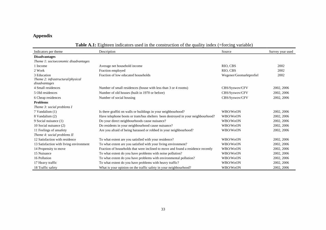
The PCA ‘quality’ index was constructed by making use of eighteen different items. These

items cover socioeconomic disadvantages, physical disadvantages, and a range of social

problems, such as nuisance, vandalism or insecurity, but also social problems in terms of poor

housing, environmental pollution, heavy traffic, noise pollution and a lack of safety. The

items were both based on measured socioeconomic variables and information about the

housing quality and obtained through surveys about nuisance and feelings of insecurity

among residents (see Table A.1 in the Appendix). The scores on this index were collected at

the PCA level. The ranking of PCAs was used to construct and thereafter select the most

disadvantaged neighbourhoods. There are approximately 4,000 PCAs in the Netherlands.

The area of a single PCA is not always considered to define a neighbourhood. In many cases

multiple, geographically adjacent PCAs form neighbourhoods. Together the selected PCAs

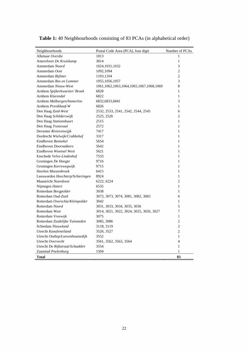
formed 40 neighbourhoods that consist of 83 PCAs. This number of 40 was – according to the

responsible politicians – a sound number of neighbourhoods to be able to guarantee a

sufficiently large monetary investment, to carefully monitor progress and to pay regular visits.

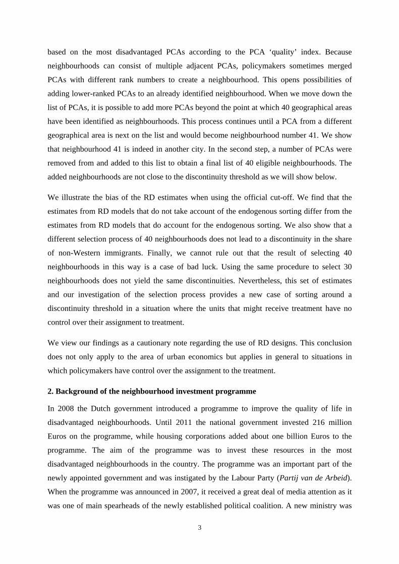
Table 1 shows the list of the 40 disadvantaged neighbourhoods and the 83 PCAs they consist

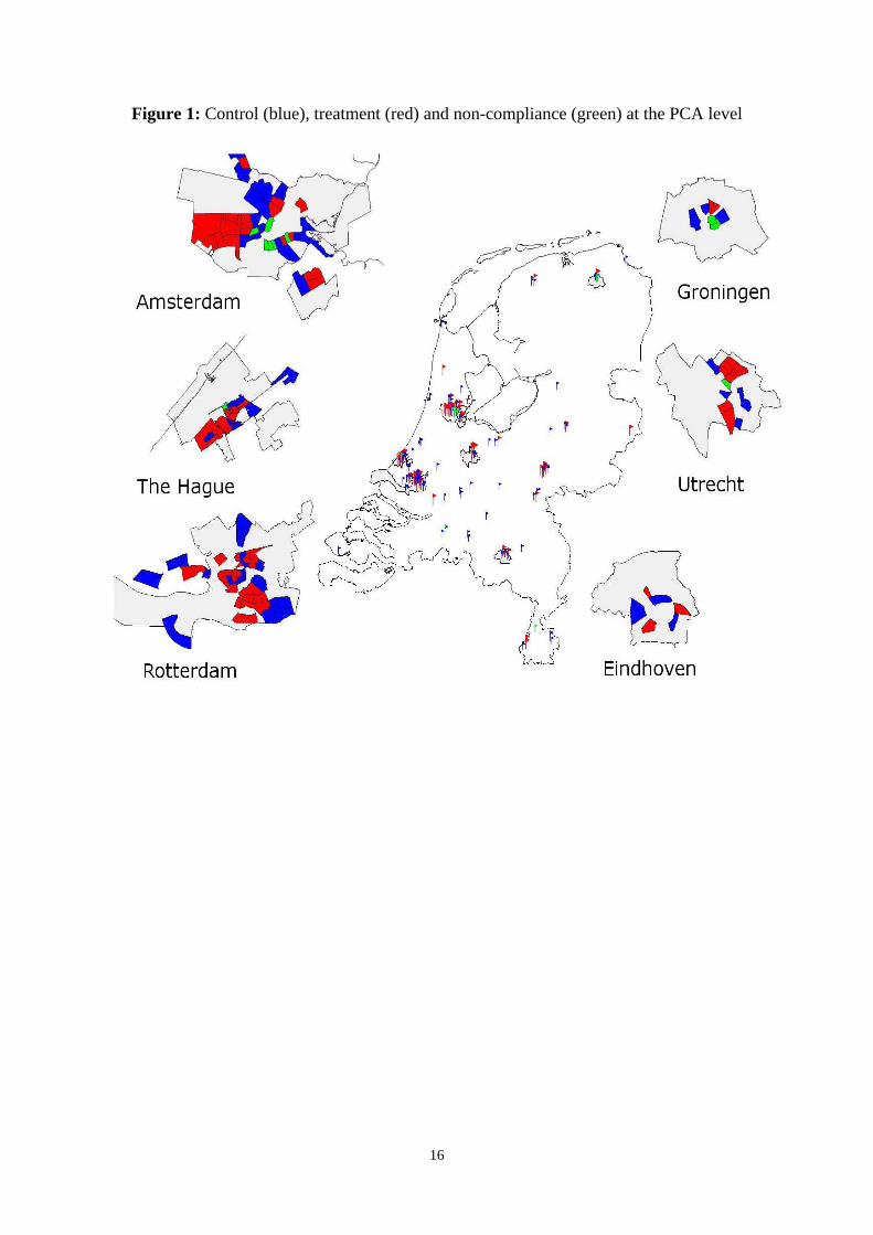
of. Figure 1 shows a map of the Netherlands in which the 83 treated PCAs are highlighted in

red. In most cases, disadvantaged neighbourhoods (PCAs) are located in the largest cities of

the country. The vast majority of the neighbourhoods is concentrated in the four largest cities

5  

in the Randstad (i.e., Amsterdam, Rotterdam, The Hague and Utrecht). The PCAs in blue and

green are control and non-compliance areas, respectively. We explain them below.

2.2. The process of selecting neighbourhoods

The consequence of the political decision to merge 83 PCAs to arrive at a number of 40

neighbourhoods is that PCAs with consecutive rank numbers (on the ‘quality’ index) are not

necessarily geographically adjacent to each other. In most cases a neighbourhood consists of

multiple PCAs with different rank numbers. Moreover, the geographical boundaries of (a

collection of) PCAs yields neighbourhoods that do often not correspond to the official

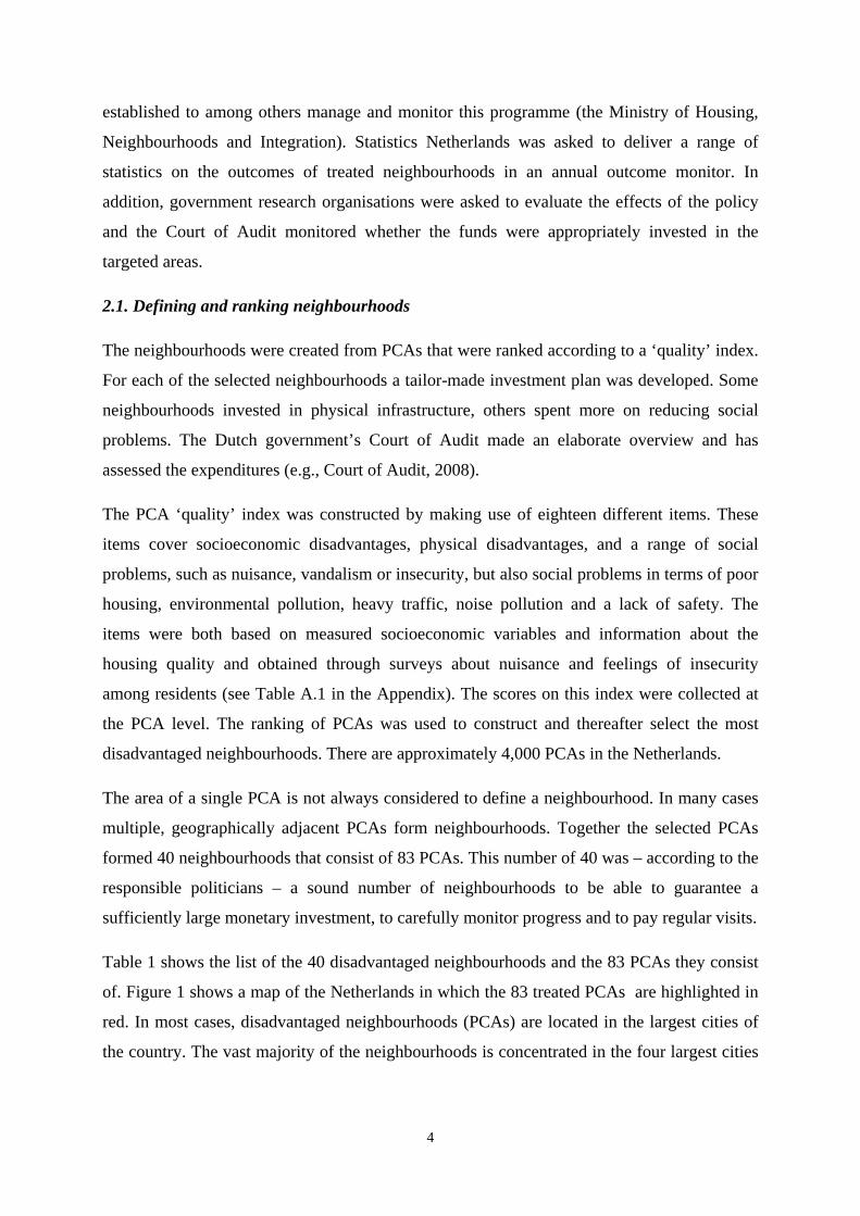
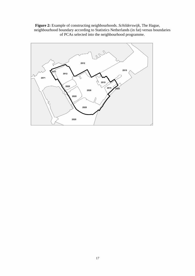
classification of neighbourhoods as defined by Statistics Netherlands (CBS). Figure 2 shows

an example. It displays the neighbourhood Schilderswijk in the Hague, which, according to

Table 1, consists of PCAs 2525 and 2526. The fat solid line depicts the geographical

boundary of the neighbourhood according to the official classification of CBS. The thin solid

lines depicts the boundaries of the PCAs. As can be seen, the lines do not coincide. Moreover,

the neighbourhood not only consists of PCAs 2525 and 2526, but also of a number of other

PCAs. Also, parts of the PCAs 2525 and 2526 do not lie in the Schilderswijk.

The process to construct 40 neighbourhoods involved two steps. First, 40 neighbourhoods

were constructed by moving down the list of PCAs. Since these neighbourhoods do not

necessarily coincide with the official classifications of Statistics Netherlands but consist of

adjacent PCAs, it is difficult to precisely reconstruct the exact scope of these initial 40

neighbourhoods. In the second step, policymakers removed and added PCAs to the list to

arrive at a final list of 40 neighbourhoods.

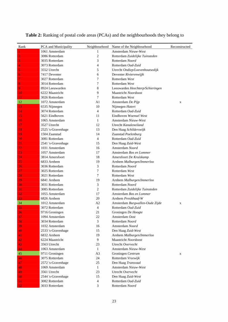
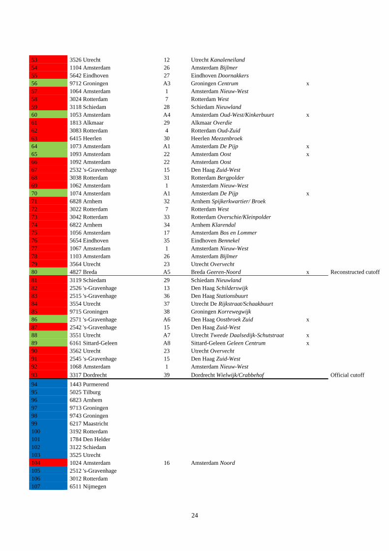
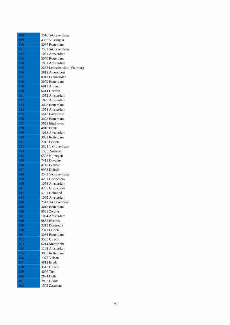
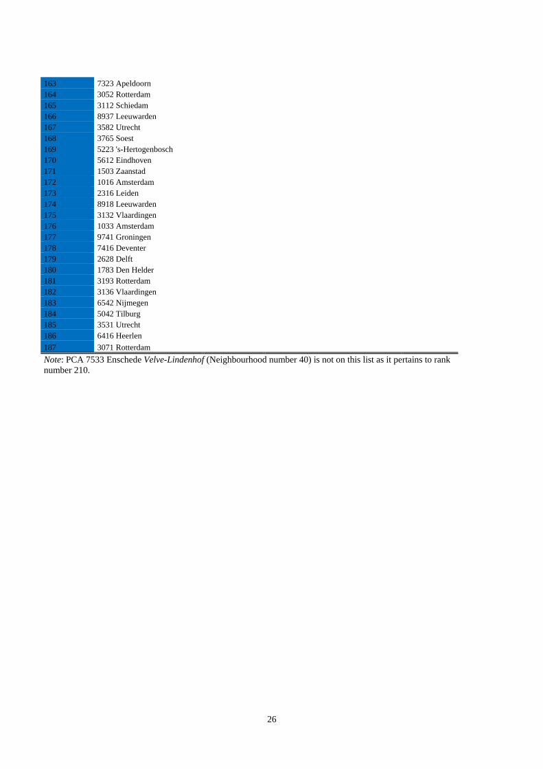
Table 2 shows the results. The table documents the worst 187 PCAs in the Netherlands

according to the ‘quality’ index (we discuss the most salient details of the index in Section 3).

The first two columns display the rank number and PCA (the higher the rank, the worse the

score on the ‘quality’ index). The third column shows the number of the neighbourhood the

PCA has been assigned to. The fourth column displays the neighbourhood’s name. The fifth

column marks whether the PCA has been removed in the first step of the selection process.

We link these PCAs to a neighbourhood just as the policymakers linked the non-removed

PCAs to neighbourhoods. That is, we reconstruct the preliminary list from the first step. If we

move down Table 2, at least four observations stand out.

6  

First, and consistent with Figure 1, a number of PCAs have been put together to form one

neighbourhood. For instance 3086 (rank 2) and 3085 (rank 31) in Rotterdam form one

neighbourhood (Zuidelijke Tuinsteden). This selection rule to define neighbourhoods leads to

putting together PCAs into neighbourhoods until the 41st neighbourhood needs to be defined.

Second, the official cut-off is set at rank 93. Policymakers arrived at this point after removing

12 and adding 2 PCAs to the list in the second step of the selection process. The 12 removed

PCAs are coloured green in Table 2. These areas are mostly touristic centres in which there is

nuisance in terms of traffic and environmental pollution. We linked these PCAs to a

neighbourhood. PCAs 7533 and 1024 have been added to the list.3 As can be seen, the cut-off

lies at the point where 39 neighbourhoods have been identified. Including 7533 (Enschede

Velve-Lindenhof) yields the 40th neighbourhood. PCA 1024 belongs to Amsterdam Noord,

which was already defined. This shows the tendency of adding PCAs to already existing

neighbourhoods.

Third, if the selection rule to define neighbourhoods was such that each single PCA would

have been considered a neighbourhood, the point at which we can identify 40

‘neighbourhoods’, would have been at rank 40 (just after 2533 Den Haag Zuid-West).

Fourth, if we allow for the combination of adjacent PCAs into a single neighbourhood, and do

not remove the twelve PCAs as the policymakers did in the second step, we arrive for the first

time at 40 neighbourhoods at rank 80 (just after including 4827 Breda Geeren-Noord). Both

‘reconstructed’ cut-offs are different from the official cut-off. We analyse the outcomes of

using different selection rules in Section 5.

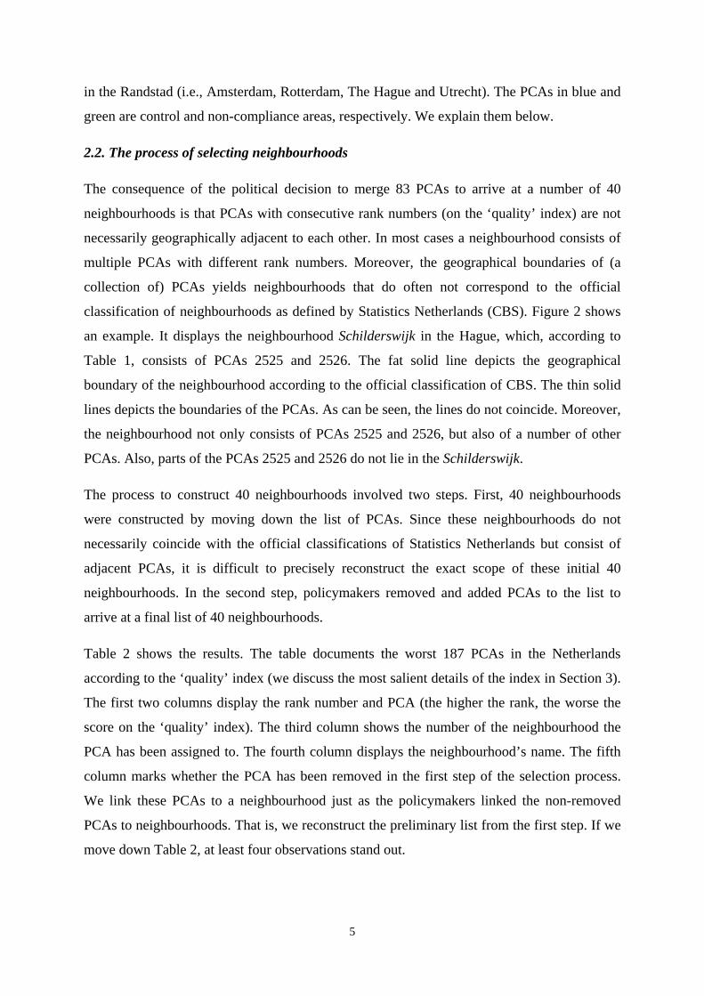
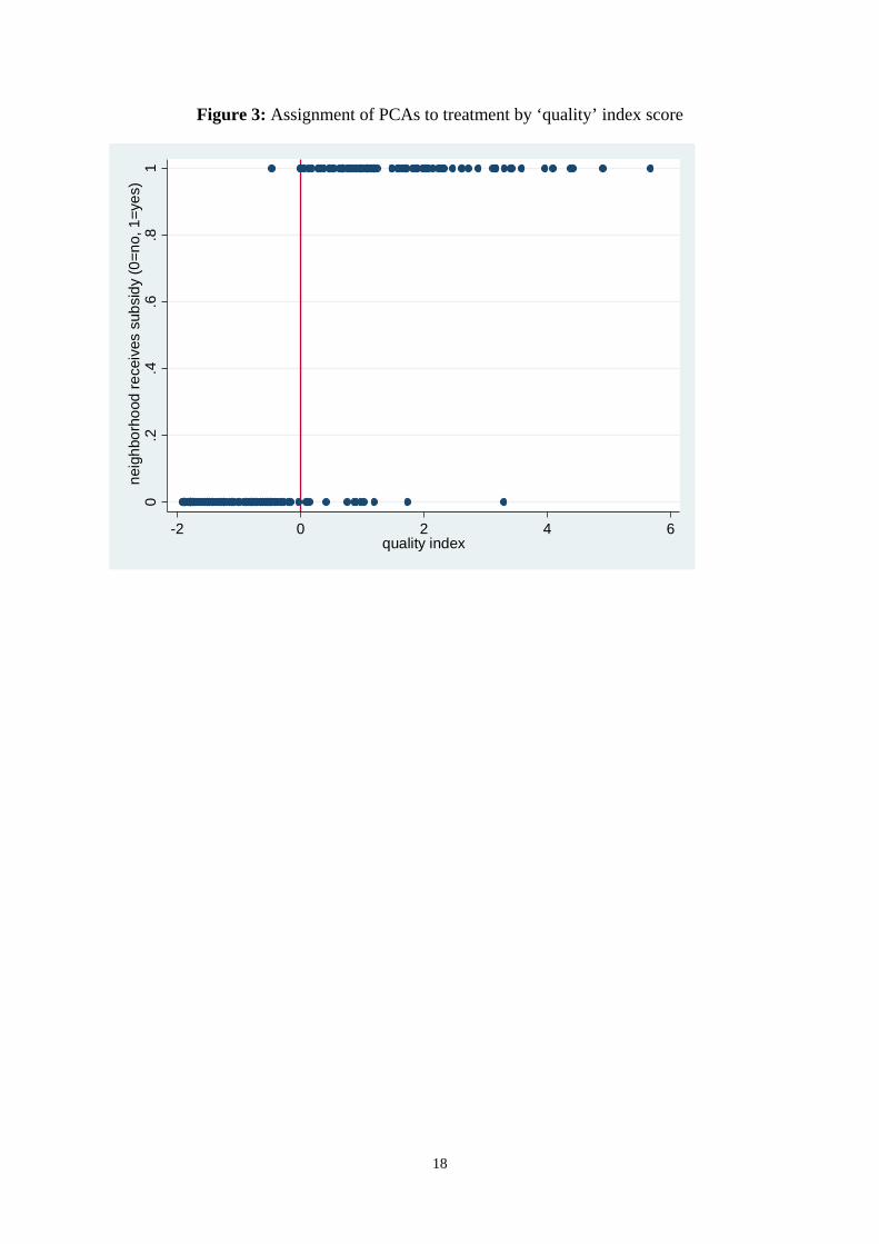
Finally, Figure 3 shows the relationship between the (scaled) ‘quality’ index of PCAs and the

actual participation in the programme using the official cut-off (at row number 93). PCAs

with scores above 0 are eligible to participate in the treatment, while PCAs with scores below

0 are not. Compliance and non-compliance with this assignment rule can be observed from

Figure 3. The 12 PCAs with a score on the ‘quality’ index that would justify treatment, but

have not been selected into the treatment, are shown at the bottom of the horizontal axis with

scores above 0. PCA 1024 Amsterdam with a negative score on the ‘quality’ index that would

not justify treatment lies to the left of cut-off at the top of the horizontal axis. PCA 7533 has

also been added to the treatment, but is not displayed in this figure because it has a very low

score on the assignment variable ( 2.3) and ranks 210th. It lies far to the left of the cut-off.                                                             3 7533 Enschede Velve-Lindenhof is not visible in Table 2 because this PCA has rank number 210.

7  

3. Data

The data for our empirical analysis are obtained from various sources. First, the ranking of

PCAs and the score on the ‘quality’ index were obtained from ABF Research, the

organisation that was asked by the government to construct the index. The ‘quality’ index will

be used as the forcing variable for the assignment of PCAs to the programme in the RD

model. We rescaled this variable in such a way that neighbourhoods with scores above 0 are

eligible, while neighbourhoods with scores below 0 are not.

Second, we obtained information on seven outcome measures from the Ministry of Housing,

Spatial Planning and the Environment: an index for the quality of life; the quality of the

public space; social cohesion; safety; quality of public services; quality of the composition of

the population and quality of the housing stock. The first measure varies between 1 and 7, and

is based on the other six measures. These vary between 50 and 50, with 0 corresponding to

the national average. The numbers do not have a clear interpretation, except that lower

numbers refer to lower quality. We obtained these measures for 2006, one year before the

start of the programme, and for 2012, four years after the start of the programme.

Third, we obtained information from Statistics Netherlands on the size and composition of the

population within PCAs: population size and the percentages of immigrants, Western-

immigrants and non-Western immigrants. Fourth, we obtained national election outcomes at

the ballot box level for 2010 and 2012.4

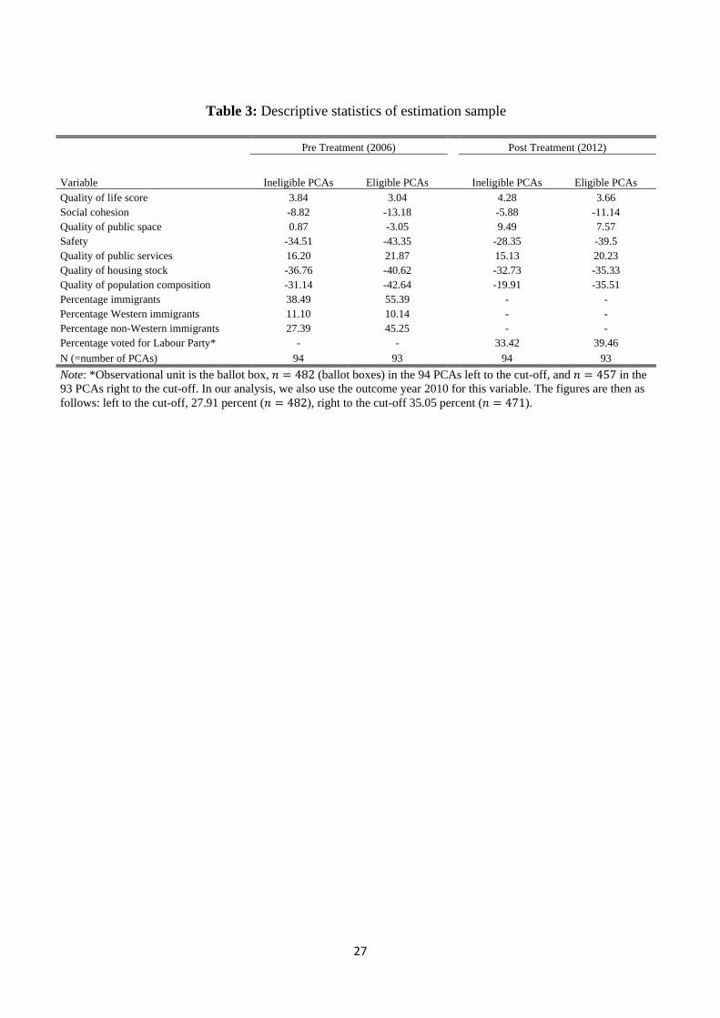
Table 3 compares the means of the outcomes and covariates for all 93 eligible PCAs to the

right of the cut-off and the same number of ineligible PCAs to the left of the cut-off.5 We

observe that in 2006, a year before the start of the programme the eligible PCAs on average

do worse on nearly all outcome measures. Moreover, these PCAs have much higher

proportions of (non-Western) immigrants. In 2012, four years after the start of the

programme, we observe a similar pattern for the differences on the outcomes variables.

4. Empirical strategy

The selection of PCAs based on the ‘quality’ index is at first sight an opportunity for applying

a RD design to evaluate the effects of the programme. The cut-off for assignment to the

                                                            4 Data from Joost Smits. For 2010: http://www.prize.nl/wiki/doku.php?id=software:databasetk2010. For 2012: http://www.prize.nl/wiki/doku.php?id=software:databasetk2012. Multiple ballot boxes can reside in one PCA. 5 We use 94 instead of 93 neighbourhoods to the left of the cut-off because two neighbourhoods have the same value of the forcing variable.

8  

treatment generates variation that is expected to be exogenous because it is beyond the control

of the treatment and control PCAs. As the central government decided about the construction

of the ‘quality’ index and because this index was not announced or available on beforehand, it

can be expected that PCAs at both sides of the cut-off will be very similar. A comparison of

the outcomes of PCAs close to the cut-off will then yield the causal effect of the

neighbourhood programme. The basic assumption in this model is that the potential outcomes

and characteristics of the PCAs are smooth around the cut-off.

This basic assumption can be investigated by performing balancing tests for the similarity of

covariates or outcome variables before the start of the programme across the cut-off. These

tests can be carried out by using a reduced form model as specified in equation (1):

(1) 0 1 ( )i i iY Z f I ,

where iY is an outcome or covariate before the start of the programme of PCA i, iZ is a

dummy variable that equals 1 if the ‘quality’ index is >0 and 0 if the ‘quality’ index is <0, and

i are unobserved factors. (.)f is a smooth function of the ‘quality’ index, which is allowed

to be different at either side of the cut-off ( lf  and rf ), as suggested by Lee and Lemieux

(2010), i.e. )]()([)()( iliriili IfIfPIfIf . The parameter 1 reveals whether or not the

outcomes and covariates before the start of the programme are balanced across the cut-off.

Statistically insignificant estimates of this parameter can be considered as support for the

main assumption of the RD model.

If this main assumption holds, the causal effect of the programme can be estimated by making

use of specifications that are very similar to equation (1). In case of full compliance with the

assignment rule, which means that all PCAs with a ‘quality’ index score above (below) the

cut-off (don’t) enrol into the programme, the effect of the programme can be estimated using

the following specification:

(2) iiii XIfPY 210 )( ,

where iY is the outcome of PCA i, iP is a dummy variable for treatment, iX is a vector of

control variables and i are unobserved factors. The main parameter for estimation is 1 ,

which can be interpreted as the causal effect of the treatment on the outcomes. Identification

9  

of 1 is based on the non-linear relationship between the ‘quality’ index and the allocation of

resources around the cut-off.

However, the selection of PCAs into the programme did not fully comply with the assignment

rule. This non-compliance can be dealt with in an instrumental variable (IV) approach. The

causal effect of the programme can be estimated by using the dummy for the assignment rule

( iZ ) as an instrument for participation in the programme ( iP ) in a two-stage least squares

(2SLS) approach. The first and second stage equations in this approach are

(3) 0 1 2( )i i i iP Z f I X ,

(4) iiii XIfPY 210 )(ˆ ,

where iP̂ in equation (4) is the predicted probability of equation (3). Estimates of the

parameter 1 yield the causal effect of the treatment for PCAs that comply with the

assignment rule.

5. Sorting around the threshold

The empirical strategy outlined in the previous section can be applied to estimate the causal

effect of the programme when the potential outcomes behave smoothly around the cut-off for

the assignment of the treatment.

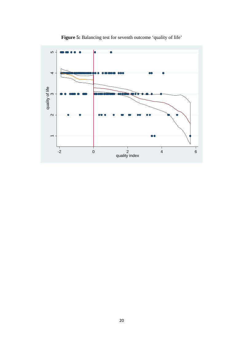
To investigate this assumption we perform balancing tests for seven outcome variables

measured a year before the start of the programme and for three covariates. For the balancing

test, we estimate the reduced form model (equation (1)). To estimate the causal effects of the

programme, we apply the 2SLS approach outlined in equations (3) and (4). 6

5.1. Balancing tests

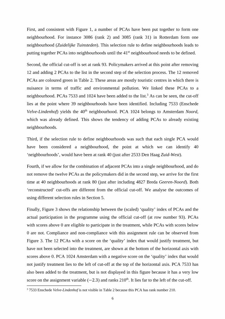
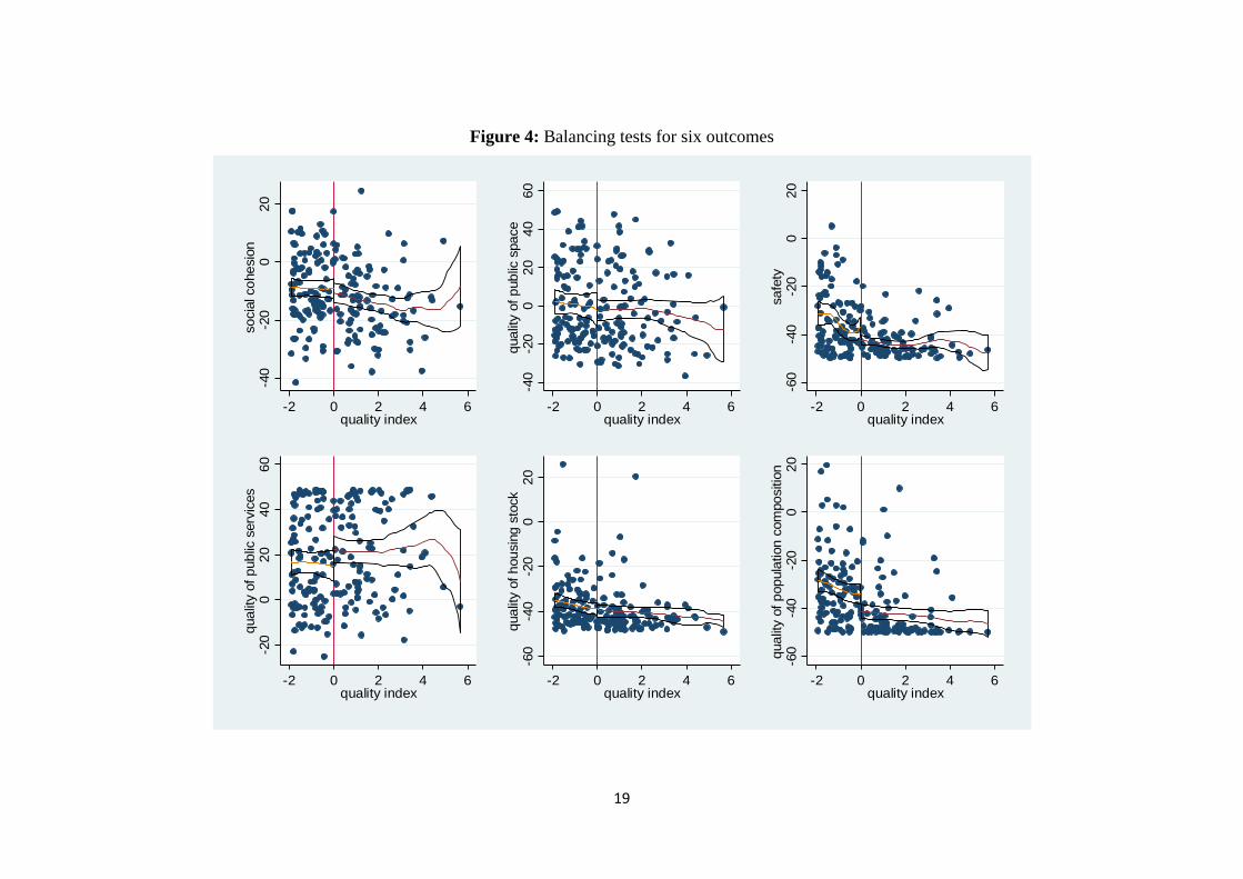
Table 4 and Figure 4 show the results of the balancing tests for the seven main outcomes

variables that have been used to build the ‘quality’ index. We use a sample of 187 PCAs that

includes all 93 PCAs to the right of the discontinuity threshold and 94 PCAs to the left of the

cut-off. For each outcome in Table 4 we use a specification with a linear and square term of

the forcing variable. We find that all reduced-form estimates are statistically insignificant.                                                             6 In all our estimations we use the most conservative (i.e., largest) standard errors. In most cases these were obtained by only correcting for heteroskedasticity. We also experimented with clustered standard errors at the municipality level ( 39). This yields in most cases lower standard errors. The notes below each table with regression coefficients document which standard errors apply.

10  

Similar results are found when we focus on a discontinuity sample closer to the cut-off (50

PCAs to the right and 50 PCAs to the left of the cut-off). The results for the seventh outcome

variable ‘quality of life’, which is based on the six outcomes used in Table 4, are also

statistically insignificant (see last column in Table 4 and Figure 5). These findings suggest

that the allocation of PCAs around the threshold is random, which supports the possibility and

usefulness of applying a RD design.

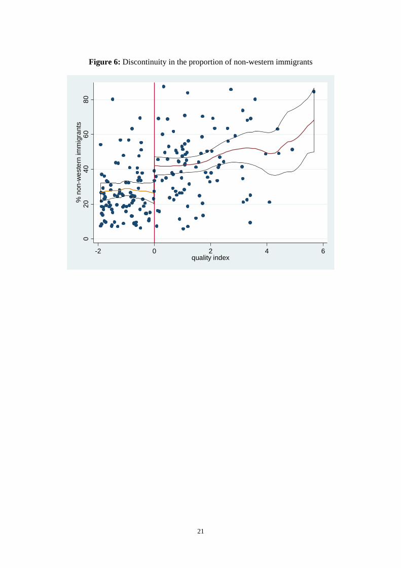
Next to the indicators that should reveal information about the ‘quality’ of the neighbourhood,

the composition of the population seems a natural indicator to investigate. Many of the PCAs

that are selected into the treatment are located in the larger cities in the Randstad. It is well-

known that the population composition in these cities is different from cities outside this area.

This does not have to be a problem if the comparison in the RD framework is between PCAs

with similar characteristics, something we expect if the variation around the cut-off is as good

as random. However, inspection of indicators of the composition of the population suggest a

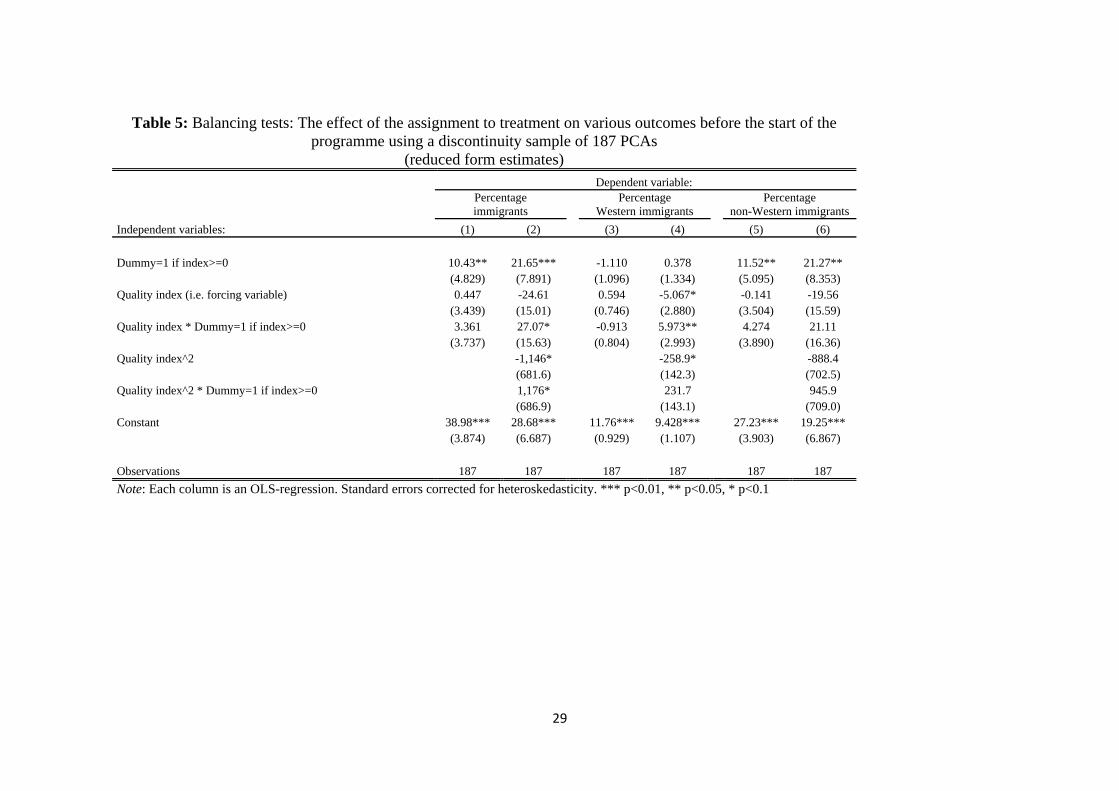
remarkable difference between the treatment and control PCAs at the cut-off. Table 5 shows

balancing tests for three indicators of the composition of the population, which have

somewhat surprisingly not been included in the ‘quality’ index. Depending on the

specification, we observe that in 2006 there are living between 11 and 21 percentage points

more non-Western immigrants in PCAs in the treatment group compared to PCAs in the

control group. 7 For the smaller discontinuity sample of 100 PCAs we observe similar

differences in the composition of the population. This gap in the proportion of non-Western

immigrants implies a large increase of this proportion at the cut-off, as shown in Figure 6. The

observed difference in the composition of the population implies that the basic assumption

about smoothness around the discontinuity is unlikely to hold.

5.2. Non-compliance with the assignment rule

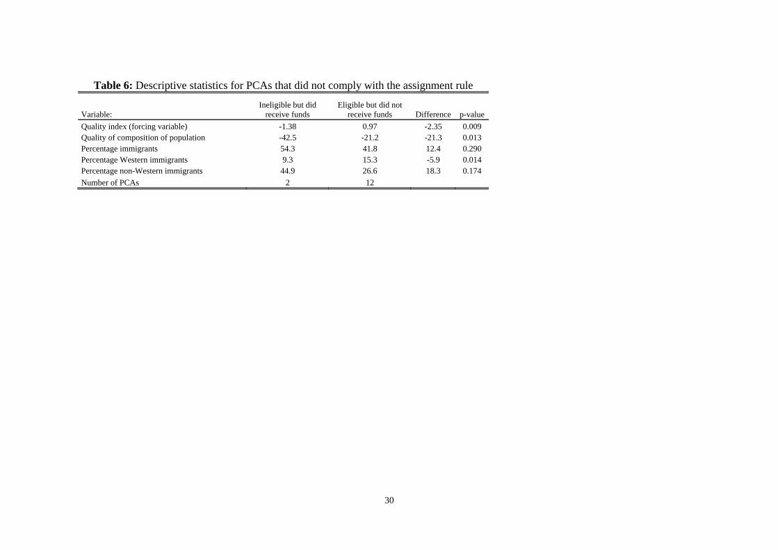
We next look at non-compliance of PCAs with the assignment rules. Twelve PCAs were

eligible for participation but were excluded; two PCAs were ineligible but did receive the

treatment. Table 6 shows descriptive statistics for these two groups. The first row shows that

the two PCAs that were ineligible do better on the ‘quality’ index. It should also be noted that

one of these two PCAs ranked as PCA number 210 in the original ranking. The second row in

Table 6 shows however that the ‘quality of the composition of the population’ differs

                                                            7 Non-western immigrants make up 11 percent of the Dutch population in 2006. The large majority of non-western immigrants are from Morocco, Turkey, Surinam and the Antilles.

11  

statistically significant between the PCAs that did receive funds and the PCAs that were

eligible but did not receive funds. Two of the other population indicators ‘percentage

immigrants’ and ‘percentage non-Western immigrants’ show the same picture. This pattern of

non-compliance is similar when compared to the previous findings from the balancing tests.

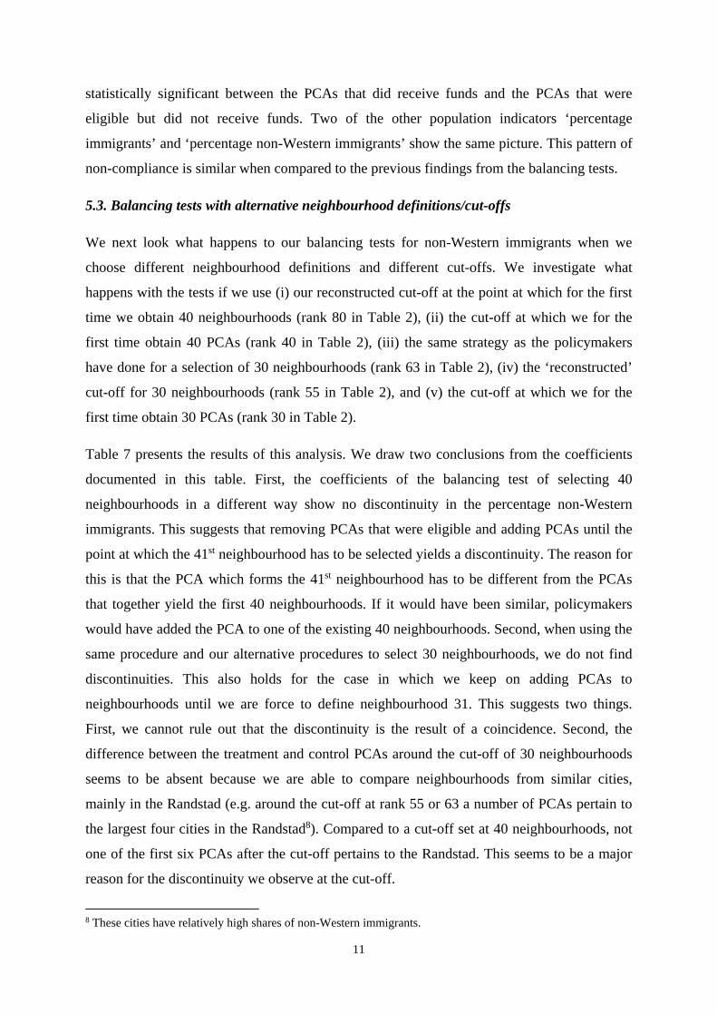
5.3. Balancing tests with alternative neighbourhood definitions/cut-offs

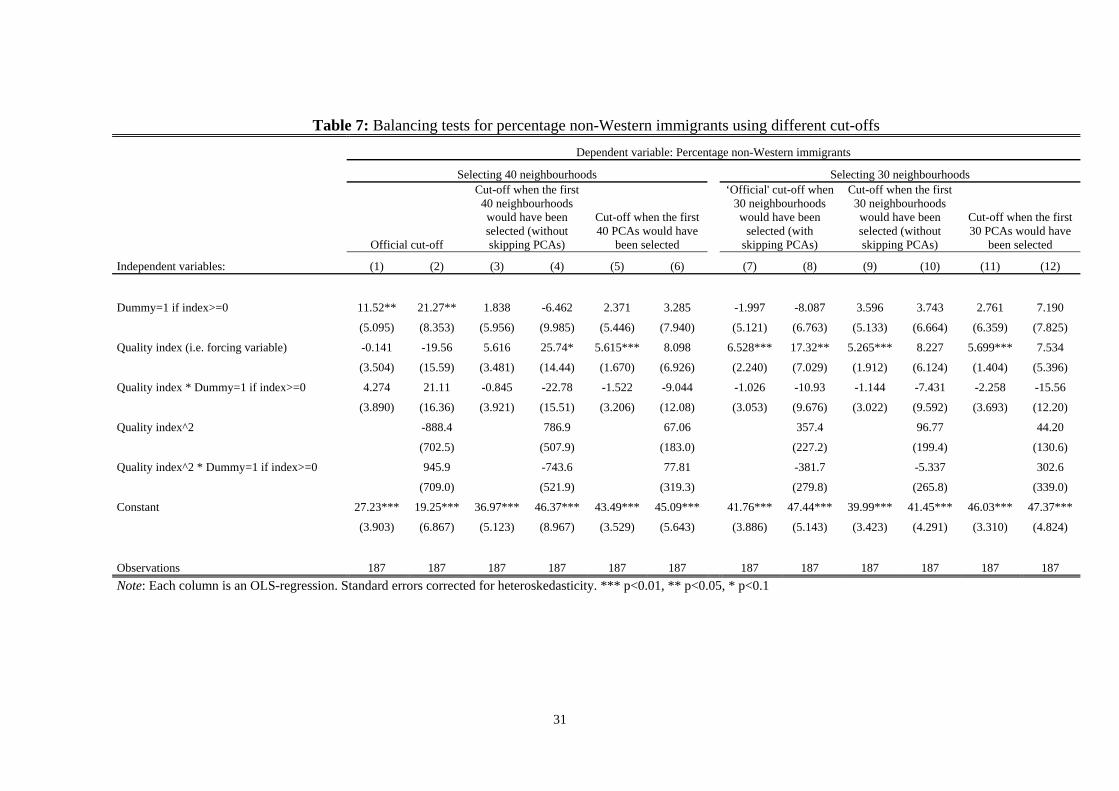
We next look what happens to our balancing tests for non-Western immigrants when we

choose different neighbourhood definitions and different cut-offs. We investigate what

happens with the tests if we use (i) our reconstructed cut-off at the point at which for the first

time we obtain 40 neighbourhoods (rank 80 in Table 2), (ii) the cut-off at which we for the

first time obtain 40 PCAs (rank 40 in Table 2), (iii) the same strategy as the policymakers

have done for a selection of 30 neighbourhoods (rank 63 in Table 2), (iv) the ‘reconstructed’

cut-off for 30 neighbourhoods (rank 55 in Table 2), and (v) the cut-off at which we for the

first time obtain 30 PCAs (rank 30 in Table 2).

Table 7 presents the results of this analysis. We draw two conclusions from the coefficients

documented in this table. First, the coefficients of the balancing test of selecting 40

neighbourhoods in a different way show no discontinuity in the percentage non-Western

immigrants. This suggests that removing PCAs that were eligible and adding PCAs until the

point at which the 41st neighbourhood has to be selected yields a discontinuity. The reason for

this is that the PCA which forms the 41st neighbourhood has to be different from the PCAs

that together yield the first 40 neighbourhoods. If it would have been similar, policymakers

would have added the PCA to one of the existing 40 neighbourhoods. Second, when using the

same procedure and our alternative procedures to select 30 neighbourhoods, we do not find

discontinuities. This also holds for the case in which we keep on adding PCAs to

neighbourhoods until we are force to define neighbourhood 31. This suggests two things.

First, we cannot rule out that the discontinuity is the result of a coincidence. Second, the

difference between the treatment and control PCAs around the cut-off of 30 neighbourhoods

seems to be absent because we are able to compare neighbourhoods from similar cities,

mainly in the Randstad (e.g. around the cut-off at rank 55 or 63 a number of PCAs pertain to

the largest four cities in the Randstad8). Compared to a cut-off set at 40 neighbourhoods, not

one of the first six PCAs after the cut-off pertains to the Randstad. This seems to be a major

reason for the discontinuity we observe at the cut-off.

                                                            8 These cities have relatively high shares of non-Western immigrants.

12  

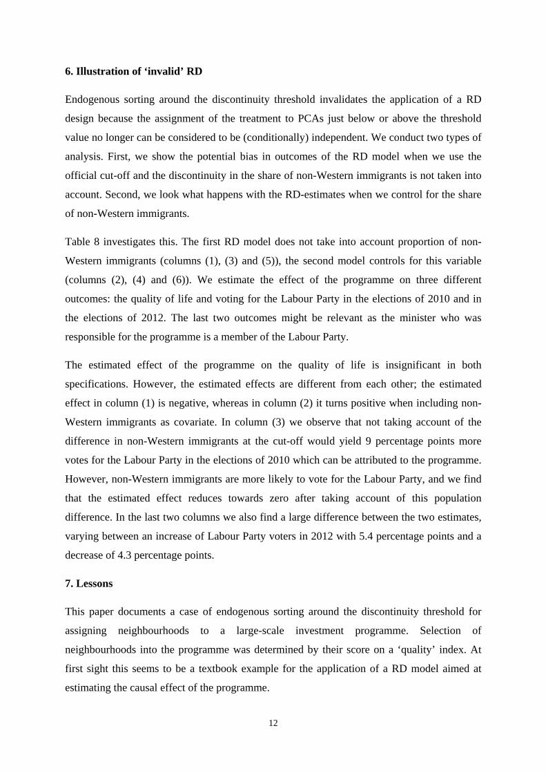
6. Illustration of ‘invalid’ RD

Endogenous sorting around the discontinuity threshold invalidates the application of a RD

design because the assignment of the treatment to PCAs just below or above the threshold

value no longer can be considered to be (conditionally) independent. We conduct two types of

analysis. First, we show the potential bias in outcomes of the RD model when we use the

official cut-off and the discontinuity in the share of non-Western immigrants is not taken into

account. Second, we look what happens with the RD-estimates when we control for the share

of non-Western immigrants.

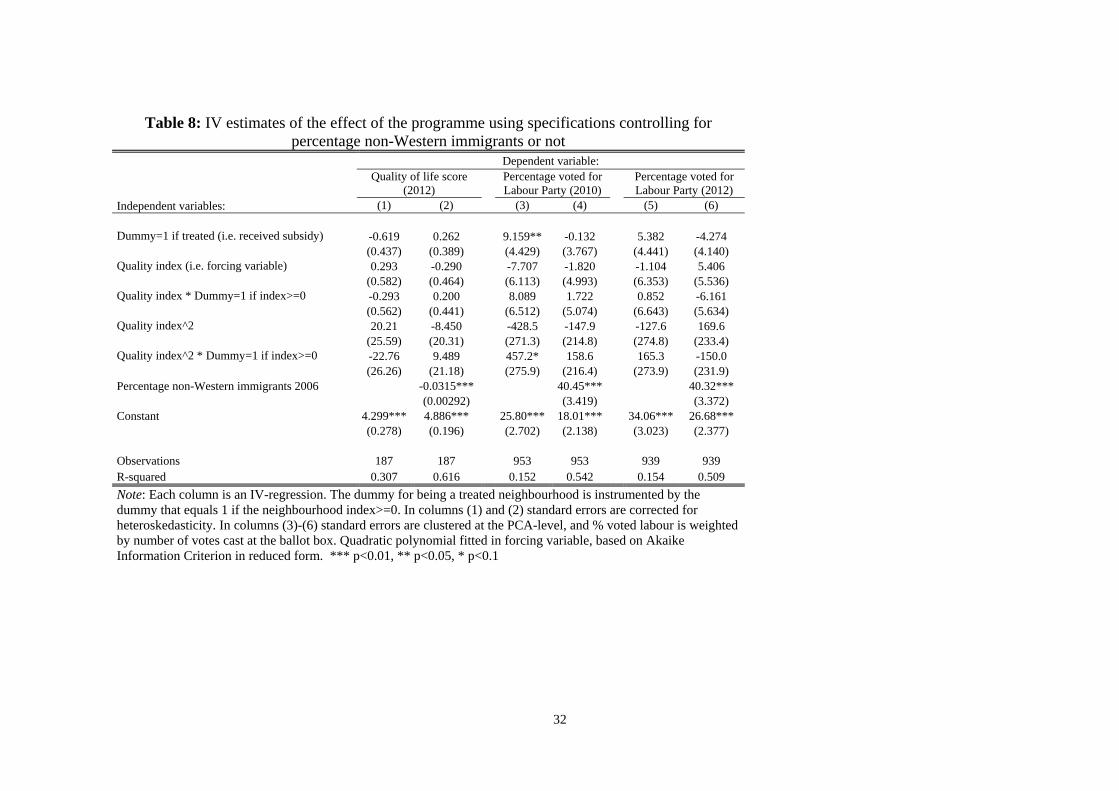
Table 8 investigates this. The first RD model does not take into account proportion of non-

Western immigrants (columns (1), (3) and (5)), the second model controls for this variable

(columns (2), (4) and (6)). We estimate the effect of the programme on three different

outcomes: the quality of life and voting for the Labour Party in the elections of 2010 and in

the elections of 2012. The last two outcomes might be relevant as the minister who was

responsible for the programme is a member of the Labour Party.

The estimated effect of the programme on the quality of life is insignificant in both

specifications. However, the estimated effects are different from each other; the estimated

effect in column (1) is negative, whereas in column (2) it turns positive when including non-

Western immigrants as covariate. In column (3) we observe that not taking account of the

difference in non-Western immigrants at the cut-off would yield 9 percentage points more

votes for the Labour Party in the elections of 2010 which can be attributed to the programme.

However, non-Western immigrants are more likely to vote for the Labour Party, and we find

that the estimated effect reduces towards zero after taking account of this population

difference. In the last two columns we also find a large difference between the two estimates,

varying between an increase of Labour Party voters in 2012 with 5.4 percentage points and a

decrease of 4.3 percentage points.

7. Lessons

This paper documents a case of endogenous sorting around the discontinuity threshold for

assigning neighbourhoods to a large-scale investment programme. Selection of

neighbourhoods into the programme was determined by their score on a ‘quality’ index. At

first sight this seems to be a textbook example for the application of a RD model aimed at

estimating the causal effect of the programme.

13  

The forcing variable was constructed from eighteen indicators on socioeconomic or housing

disadvantages, social problems and safety issues, and neighbourhoods themselves had no

control over the assignment to the treatment. However, at the cut-off for assignment to the

programme, we find a remarkably large difference in the proportion of non-Western

immigrants, a variable not taken into account in the ‘quality’ index. We also find that the

pattern of non-compliance with the assignment rule seems consistent with investing in

neighbourhoods with a high share of non-Western immigrants. These remarkable differences

cannot be explained by endogenous sorting induced by PCAs themselves, as they had no

control over the assignment to the treatment. It also seems highly unlikely that random sorting

of neighbourhoods will produce such large differences in the proportion of non-Western

immigrants at the cut-off.

We find that this non-random sorting may generate a bias of the RD estimates. Despite the

differences in the proportion of non-Western immigrants at the discontinuity threshold, both

policymakers and researchers have used the cut-off to analyse the effects of the

neighbourhood investment programme. The Ministry of Housing, Spatial Planning and the

Environment (currently the Ministry of the Interior), under which supervision the

neighbourhood investment programme was launched, has initiated several ways to review the

progress of the programme. There are several more descriptive reports available about

improvements in outcomes. These reports aim to inform members of parliament about the

progress of the programme (e.g., CBS, 2012). None of these reports have noticed or taken into

account the difference in the proportion of non-Western immigrants at the discontinuity

threshold. Also researchers did not take into account this difference at the threshold. For

example, Wittebrood and Permentier (2011) conclude that the share of non-Western

immigrants is not increasing in treatment PCAs that focussed on the restructuring of housing.

Such a finding has been regarded as a positive signal of improvement, but given our

observation that the share of non-Western immigrants was higher in the treatment PCAs

before the programme started sheds different light on this perceived success. In addition, a

recent study by Permentier et al. (2013) uses the discontinuity threshold in a RD setting to

evaluate the effects of the programme. This study does not take into account the difference in

the share of non-Western immigrants nor does it account for non-compliance with the

assignment rule.

Based on our empirical analysis we have to be careful in concluding whether or not

policymakers’ preferences or political forces at the national level have contributed to the

14  

sorting patterns observed in the data. The simplest explanation for the observed sorting

pattern is that it is a coincidence that there is such a large discontinuity in the share of non-

Western immigrants at the threshold. Indeed, several indicators have been constructed to

make a decision about which PCAs would be eligible for treatment and by coincidence there

could be a discontinuity in the share of non-Western immigrants at exactly this threshold. Our

analysis of the alternative of selecting 30 neighbourhoods with the same criterion does not

rule out this possibility.

However, some observations suggest otherwise. First, the pattern of non-compliance with the

assignment rule is consistent with selecting PCAs with more or less non-Western immigrants

into and out of the treatment, respectively. Second, the size of the difference at the threshold

points at selecting neighbourhoods in the Randstad relative to neighbourhoods in large cities

in other parts of the country. Non-Western immigrants are concentrated in the Randstad. This

selection seems to be the result of the selection rule to keep on adding PCAs to

neighbourhoods until the threshold of 40 neighbourhoods set by the Minister was exhausted.

Overall, our results provide a new case of endogenous sorting around a threshold in a

situation where the units that might receive treatment have no control over their assignment to

the treatment. We view our findings as a cautionary note regarding the use of RD designs in

situations in which policymakers are able to influence the assignment to the treatment.

References

Angrist, Joshua D., and Jörn-Steffen Pischke. 2009. Mostly Harmless Econometrics: An Empiricist’s Companion. Princeton University Press: Princeton, NJ.

Angrist, Joshua D., and Jörn-Steffen Pischke. 2010. “The Credibility Revolution in Empirical Economics: How Better Research Design Is Taking the Con out of Econometrics.” Journal of Economic Perspectives, 24(2): 3-30.

Bayer, Patrick, Fernando Ferreira, and Robert McMillan. 2007. “A Unified Framework for Measuring Preferences for Schools and Neighborhoods.” Journal of Political Economy, 115(4): 588-638.

Bubb, Ryan, and Alex Kaufman. 2014. “Securitization and Moral Hazard: Evidence from a Lender Cutoff Rule.” Journal of Monetary Economics, 63(1): 1-18.

Busso, Matias, Jesse Gregory, and Patrick Kline. 2013. “Assessing the Incidence and Efficiency of a Prominent Place Based Policy.” American Economic Review, 103(2): 897-947.

CBS. 2012. Outcomemonitor Wijkenaanpak. Statistics Netherlands: The Hague. Court of Audit. 2008. Krachtwijken. Monitoring en Verantwoording van het Beleid.

Algemene Rekenkamer: The Hague. Freedman, Matthew. 2015. “Place-Based Programs and the Geographic Dispersion of

Employment.” Regional Science and Urban Economics, 53: 1-19.

15  

Glaeser, Edward L., and Joshua D. Gottlieb. 2008. “The Economics of Place-Making Policies.” Brookings Papers on Economic Activity: 155-239.

Hahn, Jinyong, Petra Todd, and Wilbert van der Klaauw. 2001. “Identification and Estimation of Treatment Effects with a Regression-Discontinuity Design.” Econometrica, 69(1): 201-209.

Horn, Keren Mertens. 2015. “Can Improvements in Schools Spur Neighborhood Revitalization? Evidence from Building Investments.” Regional Science and Urban Economics, 52: 108-118.

Lee, David S. 2008. “Randomized Experiments from Non-Random Selection in US House Elections.” Journal of Econometrics, 142(2): 675-697.

Lee, David S., and Thomas Lemieux. 2010. “Regression Discontinuity Designs in Economics.” Journal of Economic Literature, 48(2): 281-355.

McCrary, Justin. 2008. “Manipulation of the Running Variable in the Regression Discontinuity Design: A Density Test.” Journal of Econometrics, 142(2): 698-714.

Permentier, Matthieu, Jeanet Kullberg and Lonneke van Noije. 2013. Werk aan de Wijk: Een Quasi-Experimentele Evaluatie van het Krachtwijkenbeleid. Sociaal en Cultureel Planbureau: The Hague.

Saez, Emmanuel. 2010. “Do Taxpayers Bunch at Kink Points?” American Economic Journal: Economic Policy, 2(3): 180-212.

Urquiola, Miguel, and Eric A. Verhoogen. 2009. “Class-Size Caps, Sorting, and the Regression-Discontinuity Design.” American Economic Review, 99(1): 179-215.

Vogl, Tom S. 2014. “Race and the Politics of Close Elections.” Journal of Public Economics, 109(1): 101-113.

Wittebrood, Karin, and Matthieu Permentier. 2011. Wonen, Wijken en Interventies: Krachtwijkenbeleid in Perspectief. Sociaal en Cultureel Planbureau: The Hague.

16  

Figure 1: Control (blue), treatment (red) and non-compliance (green) at the PCA level

17  

Figure 2: Example of constructing neighbourhoods. Schilderswijk, The Hague, neighbourhood boundary according to Statistics Netherlands (in fat) versus boundaries

of PCAs selected into the neighbourhood programme.

18  

Figure 3: Assignment of PCAs to treatment by ‘quality’ index score

0.2

.4.6

.81

nei

ghbo

rho

od r

ece

ives

sub

sid

y (0

=n

o, 1

=ye

s)

-2 0 2 4 6quality index

19  

Figure 4: Balancing tests for six outcomes

-40

-20

020

soci

al c

ohe

sion

-2 0 2 4 6quality index

-40

-20

020

40

60

qua

lity

of p

ublic

spa

ce

-2 0 2 4 6quality index

-60

-40

-20

020

safe

ty

-2 0 2 4 6quality index

-20

020

40

60

qua

lity

of p

ublic

ser

vice

s

-2 0 2 4 6quality index

-60

-40

-20

020

qua

lity

of h

ousi

ng s

tock

-2 0 2 4 6quality index

-60

-40

-20

020

qua

lity

of p

opul

atio

n c

ompo

sitio

n

-2 0 2 4 6quality index

20  

Figure 5: Balancing test for seventh outcome ‘quality of life’

12

34

5q

ualit

y of

life

-2 0 2 4 6quality index

21  

Figure 6: Discontinuity in the proportion of non-western immigrants

   

02

04

06

08

0%

non

-we

ste

rn im

mig

rant

s

-2 0 2 4 6quality index

22  

Table 1: 40 Neighbourhoods consisting of 83 PCAs (in alphabetical order) Neighbourhoods Postal Code Area (PCA), four digit Number of PCAs

Alkmaar Overdie 1813 1 Amersfoort De Kruiskamp 3814 1 Amsterdam Noord 1024,1031,1032 3 Amsterdam Oost 1092,1094 2 Amsterdam Bijlmer 1103,1104 2 Amsterdam Bos en Lommer 1055,1056,1057 3 Amsterdam Nieuw-West 1061,1062,1063,1064,1065,1067,1068,1069 8 Arnhem Spijkerkwartier/ Broek 6828 1 Arnhem Klarendal 6822 1 Arnhem Malburgen/Immerloo 6832,6833,6841 3 Arnhem Presikhaaf-W 6826 1 Den Haag Zuid-West 2532, 2533, 2541, 2542, 2544, 2545 6 Den Haag Schilderswijk 2525, 2526 2 Den Haag Stationsbuurt 2515 1 Den Haag Transvaal 2572 1 Deventer Rivierenwijjk 7417 1 Dordrecht Wielwijk/Crabbehof 3317 1 Eindhoven Bennekel 5654 1 Eindhoven Doornakkers 5642 1 Eindhoven Woensel West 5621 1 Enschede Velve-Lindenhof 7533 1 Groningen De Hoogte 9716 1 Groningen Korrewegwijk 9715 1 Heerlen Meezenbroek 6415 1 Leeuwarden Heechterp/Schieringen 8924 1 Maastricht Noordoost 6222, 6224 2 Nijmegen Hatert 6535 1 Rotterdam Bergpolder 3038 1 Rotterdam Oud-Zuid 3072, 3073, 3074, 3081, 3082, 3083 6 Rotterdam Overschie/Kleinpolder 3042 1 Rotterdam Noord 3031, 3033, 3034, 3035, 3036 5 Rotterdam West 3014, 3021, 3022, 3024, 3025, 3026, 3027 7 Rotterdam Vreewijk 3075 1 Rotterdam Zuidelijke Tuinsteden 3085, 3086 2 Schiedam Nieuwland 3118, 3119 2 Utrecht Kanaleneiland 3526, 3527 2 Utrecht Ondiep/Loevenhoutsedijk 3552 1 Utrecht Overvecht 3561, 3562, 3563, 3564 4 Utrecht De Rijkstraat/Schaakbrt 3554 1 Zaanstad Poelenburg 1504 1

Total 83

23  

Table 2: Ranking of postal code areas (PCAs) and the neighbourhoods they belong to

Rank PCA and Municipality Neighbourhood Name of the Neighbourhood Reconstructed

1 1061 Amsterdam 1 Amsterdam Nieuw-West 2 3086 Rotterdam 2 Rotterdam Zuidelijke Tuinsteden 3 3035 Rotterdam 3 Rotterdam Noord 4 3073 Rotterdam 4 Rotterdam Oud-Zuid 5 3552 Utrecht 5 Utrecht Ondiep/Loevenhoutsedijk 6 7417 Deventer 6 Deventer Rivierenwijjk 7 3027 Rotterdam 7 Rotterdam West 8 3014 Rotterdam 7 Rotterdam West 9 8924 Leeuwarden 8 Leeuwarden Heechterp/Schieringen 10 6222 Maastricht 9 Maastricht Noordoost 11 3026 Rotterdam 7 Rotterdam West 12 1072 Amsterdam A1 Amsterdam De Pijp x 13 6535 Nijmegen 10 Nijmegen Hatert 14 3074 Rotterdam 4 Rotterdam Oud-Zuid 15 5621 Eindhoven 11 Eindhoven Woensel West 16 1065 Amsterdam 1 Amsterdam Nieuw-West 17 3527 Utrecht 12 Utrecht Kanaleneiland 18 2525 's-Gravenhage 13 Den Haag Schilderswijk 19 1504 Zaanstad 14 Zaanstad Poelenburg 20 3081 Rotterdam 4 Rotterdam Oud-Zuid 21 2541 's-Gravenhage 15 Den Haag Zuid-West 22 1031 Amsterdam 16 Amsterdam Noord 23 1057 Amsterdam 17 Amsterdam Bos en Lommer 24 3814 Amersfoort 18 Amersfoort De Kruiskamp 25 6833 Arnhem 19 Arnhem Malburgen/Immerloo 26 3036 Rotterdam 3 Rotterdam Noord 27 3025 Rotterdam 7 Rotterdam West 28 3021 Rotterdam 7 Rotterdam West 29 6841 Arnhem 19 Arnhem Malburgen/Immerloo 30 3031 Rotterdam 3 Rotterdam Noord 31 3085 Rotterdam 2 Rotterdam Zuidelijke Tuinsteden 32 1055 Amsterdam 17 Amsterdam Bos en Lommer 33 6826 Arnhem 20 Arnhem Presikhaaf-W 34 1012 Amsterdam A2 Amsterdam Burgwallen-Oude Zijde x 35 3072 Rotterdam 4 Rotterdam Oud-Zuid 36 9716 Groningen 21 Groningen De Hoogte 37 1094 Amsterdam 22 Amsterdam Oost 38 3034 Rotterdam 3 Rotterdam Noord 39 1032 Amsterdam 16 Amsterdam Noord 40 2533 's-Gravenhage 15 Den Haag Zuid-West 41 6832 Arnhem 19 Arnhem Malburgen/Immerloo 42 6224 Maastricht 9 Maastricht Noordoost 43 3563 Utrecht 23 Utrecht Overvecht 44 1063 Amsterdam 1 Amsterdam Nieuw-West 45 9711 Groningen A3 Groningen Centrum x 46 3075 Rotterdam 24 Rotterdam Vreewijk 47 2572 's-Gravenhage 25 Den Haag Transvaal 48 1069 Amsterdam 1 Amsterdam Nieuw-West 49 3561 Utrecht 23 Utrecht Overvecht 50 2544 's-Gravenhage 15 Den Haag Zuid-West 51 3082 Rotterdam 4 Rotterdam Oud-Zuid 52 3033 Rotterdam 3 Rotterdam Noord

24  

53 3526 Utrecht 12 Utrecht Kanaleneiland 54 1104 Amsterdam 26 Amsterdam Bijlmer 55 5642 Eindhoven 27 Eindhoven Doornakkers 56 9712 Groningen A3 Groningen Centrum x 57 1064 Amsterdam 1 Amsterdam Nieuw-West 58 3024 Rotterdam 7 Rotterdam West 59 3118 Schiedam 28 Schiedam Nieuwland 60 1053 Amsterdam A4 Amsterdam Oud-West/Kinkerbuurt x 61 1813 Alkmaar 29 Alkmaar Overdie 62 3083 Rotterdam 4 Rotterdam Oud-Zuid 63 6415 Heerlen 30 Heerlen Meezenbroek 64 1073 Amsterdam A1 Amsterdam De Pijp x 65 1093 Amsterdam 22 Amsterdam Oost x 66 1092 Amsterdam 22 Amsterdam Oost 67 2532 's-Gravenhage 15 Den Haag Zuid-West 68 3038 Rotterdam 31 Rotterdam Bergpolder 69 1062 Amsterdam 1 Amsterdam Nieuw-West 70 1074 Amsterdam A1 Amsterdam De Pijp x 71 6828 Arnhem 32 Arnhem Spijkerkwartier/ Broek 72 3022 Rotterdam 7 Rotterdam West 73 3042 Rotterdam 33 Rotterdam Overschie/Kleinpolder 74 6822 Arnhem 34 Arnhem Klarendal 75 1056 Amsterdam 17 Amsterdam Bos en Lommer 76 5654 Eindhoven 35 Eindhoven Bennekel 77 1067 Amsterdam 1 Amsterdam Nieuw-West 78 1103 Amsterdam 26 Amsterdam Bijlmer 79 3564 Utrecht 23 Utrecht Overvecht 80 4827 Breda A5 Breda Geeren-Noord x Reconstructed cutoff

81 3119 Schiedam 29 Schiedam Nieuwland 82 2526 's-Gravenhage 13 Den Haag Schilderswijk 83 2515 's-Gravenhage 36 Den Haag Stationsbuurt 84 3554 Utrecht 37 Utrecht De Rijkstraat/Schaakbuurt 85 9715 Groningen 38 Groningen Korrewegwijk 86 2571 's-Gravenhage A6 Den Haag Oostbroek Zuid x 87 2542 's-Gravenhage 15 Den Haag Zuid-West 88 3551 Utrecht A7 Utrecht Tweede Daalsedijk-Schutstraat x 89 6161 Sittard-Geleen A8 Sittard-Geleen Geleen Centrum x 90 3562 Utrecht 23 Utrecht Overvecht 91 2545 's-Gravenhage 15 Den Haag Zuid-West 92 1068 Amsterdam 1 Amsterdam Nieuw-West

93 3317 Dordrecht 39 Dordrecht Wielwijk/Crabbehof Official cutoff

94 1443 Purmerend 95 5025 Tilburg 96 6823 Arnhem 97 9713 Groningen 98 9743 Groningen 99 6217 Maastricht 100 3192 Rotterdam 101 1784 Den Helder 102 3122 Schiedam 103 3525 Utrecht 104 1024 Amsterdam 16 Amsterdam Noord 105 2512 's-Gravenhage 106 3012 Rotterdam 107 6511 Nijmegen

25  

108 2516 's-Gravenhage 109 4382 Vlissingen 110 3037 Rotterdam 111 2531 's-Gravenhage 112 1051 Amsterdam 113 3076 Rotterdam 114 1091 Amsterdam 115 2263 Leidschendam-Voorburg 116 3812 Amersfoort 117 8911 Leeuwarden 118 3079 Rotterdam 119 6811 Arnhem 120 6414 Heerlen 121 1052 Amsterdam 122 1097 Amsterdam 123 3078 Rotterdam 124 1054 Amsterdam 125 5643 Eindhoven 126 3023 Rotterdam 127 5652 Eindhoven 128 4816 Breda 129 1013 Amsterdam 130 3061 Rotterdam 131 2315 Leiden 132 2524 's-Gravenhage 133 1505 Zaanstad 134 6538 Nijmegen 135 7415 Deventer 136 4142 Leerdam 137 9933 Delfzijl 138 2543 's-Gravenhage 139 4201 Gorinchem 140 1058 Amsterdam 141 4205 Gorinchem 142 5701 Helmond 143 1095 Amsterdam 144 2511 's-Gravenhage 145 3015 Rotterdam 146 8031 Zwolle 147 1034 Amsterdam 148 6882 Rheden 149 3313 Dordrecht 150 2321 Leiden 151 3032 Rotterdam 152 3555 Utrecht 153 6214 Maastricht 154 1102 Amsterdam 155 3053 Rotterdam 156 1972 Velsen 157 4812 Breda 158 3512 Utrecht 159 4006 Tiel 160 2624 Delft 161 2802 Gouda 162 1502 Zaanstad

26  

163 7323 Apeldoorn 164 3052 Rotterdam 165 3112 Schiedam 166 8937 Leeuwarden 167 3582 Utrecht 168 3765 Soest 169 5223 's-Hertogenbosch 170 5612 Eindhoven 171 1503 Zaanstad 172 1016 Amsterdam 173 2316 Leiden 174 8918 Leeuwarden 175 3132 Vlaardingen 176 1033 Amsterdam 177 9741 Groningen 178 7416 Deventer 179 2628 Delft 180 1783 Den Helder 181 3193 Rotterdam 182 3136 Vlaardingen 183 6542 Nijmegen 184 5042 Tilburg 185 3531 Utrecht 186 6416 Heerlen

187 3071 Rotterdam

Note: PCA 7533 Enschede Velve-Lindenhof (Neighbourhood number 40) is not on this list as it pertains to rank number 210.

27  

Table 3: Descriptive statistics of estimation sample

Pre Treatment (2006) Post Treatment (2012)

Variable Ineligible PCAs Eligible PCAs Ineligible PCAs Eligible PCAs

Quality of life score 3.84 3.04 4.28 3.66 Social cohesion -8.82 -13.18 -5.88 -11.14 Quality of public space 0.87 -3.05 9.49 7.57 Safety -34.51 -43.35 -28.35 -39.5 Quality of public services 16.20 21.87 15.13 20.23 Quality of housing stock -36.76 -40.62 -32.73 -35.33 Quality of population composition -31.14 -42.64 -19.91 -35.51 Percentage immigrants 38.49 55.39 - - Percentage Western immigrants 11.10 10.14 - - Percentage non-Western immigrants 27.39 45.25 - - Percentage voted for Labour Party* - - 33.42 39.46

N (=number of PCAs) 94 93 94 93

Note: *Observational unit is the ballot box, 482 (ballot boxes) in the 94 PCAs left to the cut-off, and 457 in the 93 PCAs right to the cut-off. In our analysis, we also use the outcome year 2010 for this variable. The figures are then as follows: left to the cut-off, 27.91 percent ( 482), right to the cut-off 35.05 percent ( 471).

28  

Table 4: Balancing tests: The effect of the assignment to treatment on various outcomes before the start of the programme using a discontinuity sample of 187 PCAs (reduced form estimates)

Dependent variable:

Social cohesion Quality of public

space Safety

Quality of public services

Quality of housing stock

Quality of population composition

Quality of life

[-50, 50] [-50, 50] [-50,50] [-50,50] [-50,50] [-50,50] [1,7]

Independent variables: (1) (2) (3) (4) (5) (6) (7) (8) (9) (10) (11) (12) (13) (14)

Dummy=1 if index>=0 -0.931 -1.683 0.150 -3.130 -1.722 -1.789 7.385 11.15 1.942 0.606 -3.715 -5.788 -0.0743 -0.380

(3.505) (5.394) (6.014) (10.22) (2.762) (5.458) (6.084) (9.751) (2.478) (3.938) (3.410) (5.315) (0.174) (0.259) Quality index (i.e. forcing variable) -0.681 10.11 -2.199 -3.423 -5.604** -2.892 -1.454 -13.48 -3.749* -2.311 -4.723* 0.586 -0.239** 0.301

(2.390) (9.580) (3.965) (19.98) (2.241) (12.01) (3.943) (17.42) (2.010) (8.059) (2.609) (11.16) (0.102) (0.476) Quality index * Dummy=1 if index>=0 -0.971 -17.14* 1.208 7.932 5.089** 0.850 1.398 15.16 2.764 2.406 3.180 -2.298 -0.0436 -0.463

(2.634) (10.14) (4.261) (20.58) (2.321) (12.16) (4.301) (18.19) (2.074) (8.373) (2.719) (11.48) (0.123) (0.507) Quality index^2 494.0 -56.03 124.1 -550.5 65.84 243.0 24.69

(456.5) (924.1) (545.7) (770.9) (384.5) (527.8) (22.34) Quality index^2 * Dummy=1 if index>=0 -373.3 -67.42 -89.82 511.5 -90.08 -239.2 -27.39

(461.6) (929.8) (546.9) (778.8) (387.1) (530.2) (22.60) Constant -9.588*** -5.135 -1.599 -2.104 -40.79*** -39.68*** 14.57*** 9.610 -40.97*** -40.38*** -36.43*** -34.24*** 3.573*** 3.795***

(2.701) (4.346) (4.923) (9.102) (2.501) (5.125) (5.110) (8.595) (1.928) (3.359) (2.812) (4.585) (0.125) (0.195)

Observations 187 187 187 187 187 187 187 187 187 187 187 187 187 187

Note: Each column is an OLS-regression. Standard errors corrected for heteroskedasticity. *** p<0.01, ** p<0.05, * p<0.1

29  

Table 5: Balancing tests: The effect of the assignment to treatment on various outcomes before the start of the programme using a discontinuity sample of 187 PCAs

(reduced form estimates) Dependent variable:

Percentage immigrants

Percentage Western immigrants

Percentage non-Western immigrants

Independent variables: (1) (2) (3) (4) (5) (6)

Dummy=1 if index>=0 10.43** 21.65*** -1.110 0.378 11.52** 21.27** (4.829) (7.891) (1.096) (1.334) (5.095) (8.353)

Quality index (i.e. forcing variable) 0.447 -24.61 0.594 -5.067* -0.141 -19.56 (3.439) (15.01) (0.746) (2.880) (3.504) (15.59)

Quality index * Dummy=1 if index>=0 3.361 27.07* -0.913 5.973** 4.274 21.11 (3.737) (15.63) (0.804) (2.993) (3.890) (16.36)

Quality index^2 -1,146* -258.9* -888.4 (681.6) (142.3) (702.5)

Quality index^2 * Dummy=1 if index>=0 1,176* 231.7 945.9 (686.9) (143.1) (709.0)

Constant 38.98*** 28.68*** 11.76*** 9.428*** 27.23*** 19.25*** (3.874) (6.687) (0.929) (1.107) (3.903) (6.867)

Observations 187 187 187 187 187 187

Note: Each column is an OLS-regression. Standard errors corrected for heteroskedasticity. *** p<0.01, ** p<0.05, * p<0.1

   

30  

Table 6: Descriptive statistics for PCAs that did not comply with the assignment rule

Variable: Ineligible but did

receive funds Eligible but did not

receive funds Difference p-value

Quality index (forcing variable) -1.38 0.97 -2.35 0.009 Quality of composition of population -42.5 -21.2 -21.3 0.013 Percentage immigrants 54.3 41.8 12.4 0.290 Percentage Western immigrants 9.3 15.3 -5.9 0.014 Percentage non-Western immigrants 44.9 26.6 18.3 0.174

Number of PCAs 2 12

 

31  

Table 7: Balancing tests for percentage non-Western immigrants using different cut-offs

Dependent variable: Percentage non-Western immigrants

Selecting 40 neighbourhoods Selecting 30 neighbourhoods

Official cut-off

Cut-off when the first 40 neighbourhoods would have been selected (without skipping PCAs)

Cut-off when the first 40 PCAs would have

been selected

‘Official' cut-off when 30 neighbourhoods would have been

selected (with skipping PCAs)

Cut-off when the first 30 neighbourhoods would have been selected (without skipping PCAs)

Cut-off when the first 30 PCAs would have

been selected

Independent variables: (1) (2) (3) (4) (5) (6) (7) (8) (9) (10) (11) (12)

Dummy=1 if index>=0 11.52** 21.27** 1.838 -6.462 2.371 3.285 -1.997 -8.087 3.596 3.743 2.761 7.190

(5.095) (8.353) (5.956) (9.985) (5.446) (7.940) (5.121) (6.763) (5.133) (6.664) (6.359) (7.825)

Quality index (i.e. forcing variable) -0.141 -19.56 5.616 25.74* 5.615*** 8.098 6.528*** 17.32** 5.265*** 8.227 5.699*** 7.534

(3.504) (15.59) (3.481) (14.44) (1.670) (6.926) (2.240) (7.029) (1.912) (6.124) (1.404) (5.396)

Quality index * Dummy=1 if index>=0 4.274 21.11 -0.845 -22.78 -1.522 -9.044 -1.026 -10.93 -1.144 -7.431 -2.258 -15.56

(3.890) (16.36) (3.921) (15.51) (3.206) (12.08) (3.053) (9.676) (3.022) (9.592) (3.693) (12.20)

Quality index^2 -888.4 786.9 67.06 357.4 96.77 44.20

(702.5) (507.9) (183.0) (227.2) (199.4) (130.6)

Quality index^2 * Dummy=1 if index>=0 945.9 -743.6 77.81 -381.7 -5.337 302.6

(709.0) (521.9) (319.3) (279.8) (265.8) (339.0)

Constant 27.23*** 19.25*** 36.97*** 46.37*** 43.49*** 45.09*** 41.76*** 47.44*** 39.99*** 41.45*** 46.03*** 47.37***

(3.903) (6.867) (5.123) (8.967) (3.529) (5.643) (3.886) (5.143) (3.423) (4.291) (3.310) (4.824)

Observations 187 187 187 187 187 187 187 187 187 187 187 187

Note: Each column is an OLS-regression. Standard errors corrected for heteroskedasticity. *** p<0.01, ** p<0.05, * p<0.1

32  

Table 8: IV estimates of the effect of the programme using specifications controlling for percentage non-Western immigrants or not

Dependent variable: Quality of life score

(2012) Percentage voted for Labour Party (2010)

Percentage voted for Labour Party (2012)

Independent variables: (1) (2) (3) (4) (5) (6) Dummy=1 if treated (i.e. received subsidy) -0.619 0.262 9.159** -0.132 5.382 -4.274

(0.437) (0.389) (4.429) (3.767) (4.441) (4.140) Quality index (i.e. forcing variable) 0.293 -0.290 -7.707 -1.820 -1.104 5.406

(0.582) (0.464) (6.113) (4.993) (6.353) (5.536) Quality index * Dummy=1 if index>=0 -0.293 0.200 8.089 1.722 0.852 -6.161

(0.562) (0.441) (6.512) (5.074) (6.643) (5.634) Quality index^2 20.21 -8.450 -428.5 -147.9 -127.6 169.6

(25.59) (20.31) (271.3) (214.8) (274.8) (233.4) Quality index^2 * Dummy=1 if index>=0 -22.76 9.489 457.2* 158.6 165.3 -150.0

(26.26) (21.18) (275.9) (216.4) (273.9) (231.9) Percentage non-Western immigrants 2006 -0.0315*** 40.45*** 40.32***

(0.00292) (3.419) (3.372) Constant 4.299*** 4.886*** 25.80*** 18.01*** 34.06*** 26.68***

(0.278) (0.196) (2.702) (2.138) (3.023) (2.377)

Observations 187 187 953 953 939 939 R-squared 0.307 0.616 0.152 0.542 0.154 0.509

Note: Each column is an IV-regression. The dummy for being a treated neighbourhood is instrumented by the dummy that equals 1 if the neighbourhood index>=0. In columns (1) and (2) standard errors are corrected for heteroskedasticity. In columns (3)-(6) standard errors are clustered at the PCA-level, and % voted labour is weighted by number of votes cast at the ballot box. Quadratic polynomial fitted in forcing variable, based on Akaike Information Criterion in reduced form. *** p<0.01, ** p<0.05, * p<0.1

33  

Appendix

Table A.1: Eighteen indicators used in the construction of the quality index (=forcing variable) Indicators per theme Description Source Survey year used

Disadvantages Theme 1: socioeconomic disadvantages 1 Income Average net household income RIO, CBS 2002 2 Work Fraction employed RIO, CBS 2002 3 Education Fraction of low educated households Wegener/Geomarktprofiel 2002 Theme 2: infrastructural/physical disadvantages 4 Small residences Number of small residences (house with less than 3 or 4 rooms) CBS/Syswov/CFV 2002, 2006

5 Old residences Number of old houses (built in 1970 or before) CBS/Syswov/CFV 2002, 2006

6 Cheap residences Number of social housing CBS/Syswov/CFV 2002, 2006 Problems Theme 3: social problems I 7 Vandalism (1) Is there graffiti on walls or buildings in your neighbourhood? WBO/WoON 2002, 2006 8 Vandalism (2) Have telephone boots or tram/bus shelters been destroyed in your neighbourhood? WBO/WoON 2002, 2006 9 Social nuisance (1) Do your direct neighbourhoods cause nuisance? WBO/WoON 2002, 2006 10 Social nuisance (2) Do residents in your neighbourhood cause nuisance? WBO/WoON 2002, 2006 11 Feelings of unsafety Are you afraid of being harassed or robbed in your neighbourhood? WBO/WoON 2002, 2006 Theme 4: social problems II 12 Satisfaction with residence To what extent are you satisfied with your residence? WBO/WoON 2002, 2006 13 Satisfaction with living environment To what extent are you satisfied with your living environment? WBO/WoON 2002, 2006 14 Propensity to move Fraction of households that were inclined to move and found a residence recently WBO/WoON 2002, 2006 15 Nuisance To what extent do you have problems with noise pollution? WBO/WoON 2002, 2006 16 Pollution To what extent do you have problems with environmental pollution? WBO/WoON 2002, 2006 17 Heavy traffic To what extent do you have problems with heavy traffic? WBO/WoON 2002, 2006

18 Traffic safety What is your opinion on the traffic safety in your neighbourhood? WBO/WoON 2002, 2006