Sonar Implementation Concepts - Pennsylvania State … Implementation ... –signal detection ......

Applied Research Laboratory

Sonar Implementation

Concepts

Presented by: Dr. Martin A. Mazur

1


Outline

• The sonar environment

• Typical sonar block diagram

• Brief tour of some topics covered in much

greater depth in other courses:

– signal representation

– beamforming

– signal detection

• Passive processing

• Active processing

2


References • A. D. Waite, SONAR for Practising Engineers, Third Edition, Wiley (2002) (B)

• W. S. Burdic, Underwater Acoustic System Analysis, Prentice-Hall, (1991) Chapters 6-9, 11, 13, 15. (M)

• R. J. Urick, Principles of Underwater Sound, McGraw-Hill, (1983). (M)

• X. Lurton, An Introduction to Underwater Acoustics, Springer, (2002) (M)

• J. Minkoff, Signal Processing: Fundamentals and Applications for Communications and Sensing

Systems, Artech House, Boston, (2002). (M)

• Richard P. Hodges, Underwater Acoustics: Analysis, Design, and Performance of Sonar, Wiley, (2010). (M)

• Digital Signal Processing for Sonar, Knight, Pridham, and Kay, Proceedings of the IEEE, Vol. 69, No. 11,

November 1981. (M)

• M. A. Ainslie, Principles of Sonar Performance Modeling, Springer-Praxis, 2010. (A)

• H. L. Van Trees, Detection, Estimation and Modulation Theory, Part I, Wiley (1968) (A)

• J-P. Marage and Y. Mori, Sonar and Underwater Acoustics, Wiley, (2010) (A)

• Richard O. Nielsen, Sonar Signal Processing, Artech House, (1991) (A)

• B. D. Steinberg, Principles of Aperture and Array System Design, Wiley, New York (1976). (A)

(B) – Basic/Overview/Reference (M) – Mid-level/General/Reference (A) – Advanced/Special Topic

3


The Sonar Environment and the

Sonar Equation

4


Reflector / Radiator

•Radiated sound level (P,A)

•Target strength (A)

Sea Surface

•Surface reverberation (A)

•Surface ambient noise (A,P)

•Multi-path (A,P)

Sonar System

•Signal parameters (A)

•Source Level (A)

•Transmitter (A) and receiver

(A,P) directivity (beamforming)

•Signal processing gain (A,P)

•Self-Noise (A,P)

Propagation Medium

•Sound spreading and refraction (A,P)

•Absorption (A,P)

•Volume reverberation (A)

•Biological and other ambient noise (A,P)

Sea Bottom

•Bottom reverberation (A)

•Transmission loss and refraction (A)

•Multi-path (A,P)

False Targets

•Rocks, marine life (A)

Countermeasures

•Echo-repeaters (A)

•Noise makers, Jammers, (A,P)

Signals and Noise in Underwater Sonar

5


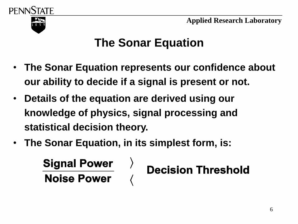
• The Sonar Equation represents our confidence about

our ability to decide if a signal is present or not.

• Details of the equation are derived using our

knowledge of physics, signal processing and

statistical decision theory.

• The Sonar Equation, in its simplest form, is:

The Sonar Equation

6


Decibels

• Sound power per unit area in an acoustic wave is sound intensity.

• For progressive plane waves, sound intensity is proportional to the square of sound pressure.

• Sound power is often expressed in decibels, and is always given in relation to some reference. So a signal level (“sound pressure level”), in dB, is related to the signal pressure:

S = 20* log10(Signal Pressure/Reference Pressure)

• The reference pressure most often used in underwater acoustics is 1 micro Pascal.

7


• Signal-to-Noise ratio SNR is sometimes referred to

the input to the sonar system (i.e. “in the water”).

• The sonar equation is usually expressed in decibels

as a difference:

• In the above,

- [S – N]in is the signal to noise ratio, expressed in dB, at the

input to the sonar system.

- DT is called the input Detection Threshold.

• The sonar equation can also be written relative to the

receiver output at the point where a detection

decision is made.

The Sonar Equation (Cont’d)

8


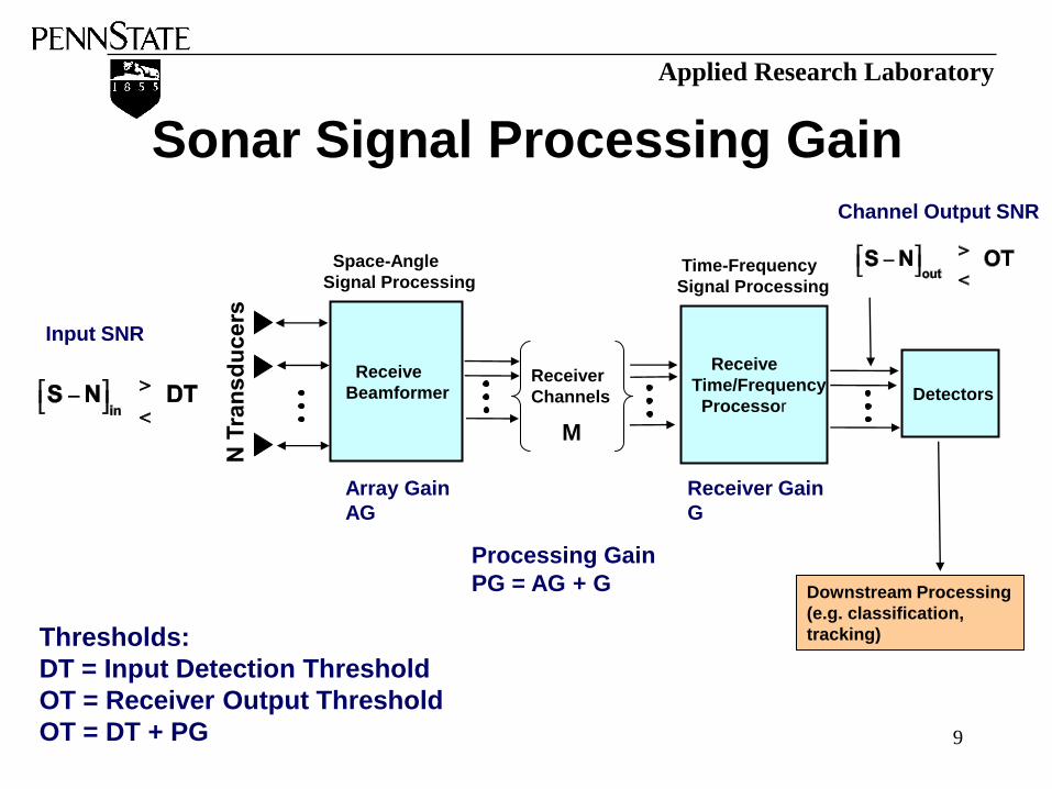
Sonar Signal Processing Gain

Detectors

Receive

Beamformer

Receive

Time/Frequency

Processor

Downstream Processing

(e.g. classification,

tracking)

Processing Gain

PG = AG + G

M

Receiver

Channels

Receiver Gain

G

Array Gain

AG

Input SNR

Channel Output SNR

Thresholds:

DT = Input Detection Threshold

OT = Receiver Output Threshold

OT = DT + PG

Space-Angle

Signal Processing Time-Frequency

Signal Processing

9


Sonar System Gains and Losses

• An active sonar transmits sound, or a passive source radiates sound, at a given source level.

• Sonar equation usually expressed in terms of SNR at some point internal to sonar system (beamformer output or receiver input).

• In analyzing the radiated or reflected sound, gains and losses intrinsic to the sonar system must be accounted for:

• Losses may include – Transmit and receive beam pointing errors’ effects on signal

– Signal processing losses (“mismatches” of all kinds)

• Gains may include – Beamforming reduction of noise (“array gain”)

– Receiver signal processing gain 10


• With

Receiver Output Threshold (OT) = Input DetectionThreshold (DT) +

Sonar Processing Gain (PG)

– OT depends on desired statistical reliability of receiver and its

design characteristics.

– PG generally depends on the sonar array characteristics, the

characteristics of the particular signal being received, and the type

of noise that predominates.

• The Sonar Equation at the receiver output becomes

where

The Sonar Equation (Cont’d)

11


Sonar Equations (Continued)

• Active Sonar: S = TL – (20*log10(R) + a*R) + TS - (20*log10(R) + a*R)

= TL – (40*log10(R) +2*a*R) + TS

where TL = transmitted level;

TS = target strength;

a = absorption loss coefficient

N = 20*log10(Nambient + Nreverb + Nself + Ntarget)

• Passive Sonar: S = SL– (20*log10(R) + a*R)

where SL = radiated level of passive source

N = 20*log10( Nambient + Nself)

12


Signal Sources

• Active: – Received signal is an attenuated and distorted version (echo) of

the transmitted signal

– “False targets” and reverberation are echoes of the transmitted

signal off of discrete and distributed environmental reflectors

• Passive – Sound radiated from a target can be from machinery, flow noise,

target sonar, and other sources

13


Attenuation

• Sound is attenuated by spreading and

absorption

– Sound spreads out geometrically from its source and

again upon reflection

– Absorption in salt water is frequency dependent.

• Higher frequencies suffer greater absorption loss.

• Absorption loss is negligible in fresh water

• Active sonar suffers a two-way attenuation loss

14


Noise Sources: Ambient

• Ambient noise is the noise that exists in a particular part of the water irrespective of the presence of the sonar or the target

• Sources: – Thermal

– Biological

– Noise from the surface: wind, waves, rain

– Shipping

• Ambient noise is location, depth, wind speed, and frequency dependent

• Simplest ambient noise model is isotropic; real ambient noise is often direction dependent

15


Noise Sources: Reverberation

• Reverberation is the echo of the transmitted signal off of the environment: – boundaries – surface and bottom reverberation

– scatterers in the water – volume reverberation

• Reverberation is directly proportional to signal energy and duration.

• Reverberation varies as 20*log(r) + 2ar (volume); 30*log(r) + 2ar (boundary)

• Due to scatterer motion, spectrum of reverberation is spread in relation to signal spectrum

16


Noise Sources: Self Noise

• Self Noise is the noise that the sonar and its vehicle make

• Sources: – Electrical – usually the lowest noise in the system

– Machinery – may be coherent from channel to channel

– Flow through the water – incoherent from channel to channel

• Flow noise is usually the dominant source of self noise for a moving sonar system

• Flow noise varies as 70*log(v/vref) (where v is the sonar platform’s velocity and vref is a reference velocity)

17


Noise Sources: Target Radiated Noise

• Target radiated noise can interfere with active

reception. Is often the means of detecting a

target passively

• Noise varies widely in strength with source type

• Noise can have a wide variety of spectral shapes

• Noise varies as 20*log(r) + ar

18


Target Echo

• The target reflects a replica of the transmitted

signal

• The echo level is proportional to the transmitted

source level.

• The proportionality “constant” is target strength

(TS), a complex measure of the sound reflecting

attributes of the target.

• Target echo varies as 40*log(r) + 2ar

• Target echo spectrum of a moving target is

doppler shifted relative to transmitted signal 19


Sonar System Block Diagram

20


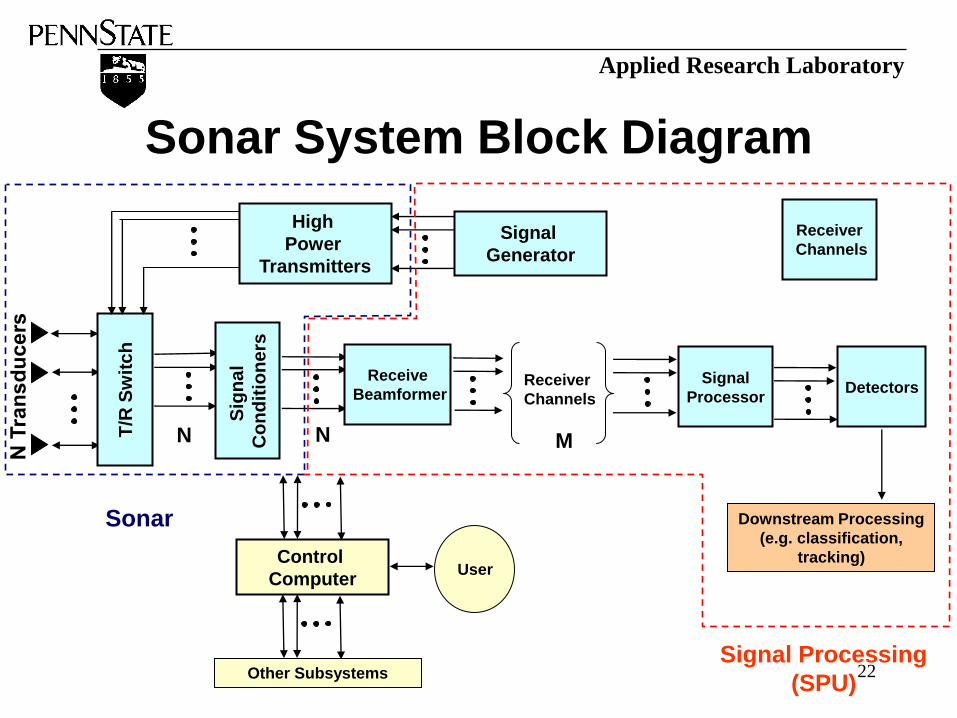
Sonar System

• A sonar system may be part of a larger

system, say an autonomous vehicle, with

other subsystems (autopilot, propulsion,

etc.)

• Sonar systems can contain both a

transmitter and receiver, sometimes using

the same transducer hardware.

• Often broken down into units of the sonar

hardware itself, and a signal processing unit

(SPU). 21


Sonar System Block Diagram

Signal

Generator

High

Power

Transmitters

Detectors

T/R

Sw

itc

h

Sig

na

l

Co

nd

itio

ne

rs

Receive

Beamformer

Receiver

Channels

Signal

Processor

Downstream Processing

(e.g. classification,

tracking) Control

Computer User

Other Subsystems

Sonar

Signal Processing

(SPU)

N N M

Receiver

Channels

22


Control Computer

• Maintains control of all sonar subsystems

• Works in concert with other subsystems,

e.g. tactical, autopilot, propulsion

• Receives and executes commands from

the user. These “commands” may be a

suite of programmed behaviors for

autonomous vehicles.

23


Transducers

• Interface between the ocean and the sonar

electronics

• Converts sound to electrical impulses and

vice-versa

• Can be a linear, planar, or volumetric array

• Transducer functions:

– Transmit

– Receive

• Many transducers perform both functions 24


Transducer Transmit Properties

• Converts electrical signals to acoustic signals

– Response given as:

pressure at a distance for a given voltage or current drive

dB re 1uPa @ 1m re 1 volt. Generally a function of frequency

• Requirements/Considerations:

– High power low impedance

– High efficiency

– Amplitude and phase matched and stable for use in

arrays

– Low ‘Q’ for wideband operation 25


Transducer Receive Properties

• Converts acoustic signals to electrical signals

– Response given as:

voltage out for a given pressure at the transducer

dBv re 1uPa. Generally a function of frequency

• Requirements/Considerations:

– High sensitivity

– Low noise

– Amplitude and phase matched and stable for use in

arrays

– Low ‘Q’ for wideband operation 26


Transmit/Receive (T/R) Switch

• Connects the transmitter to the transducer

for active transmissions

• Receiver must be protected from the high

transmit power

• T/R switch accomplishes this via switching

and isolation circuitry

• Receiver can still be susceptible to

transmitter noise coupling through T/R

switch

27


Transmit: Signal Generator

• Provides drive signals to the high power

transmitter

• Controls:

– Signal waveform generation

• amplitude

• phase (frequency)

– Multiple transmit sequencing

– Transmit beam shaping

– Transmit beam steering

– Own-Doppler nullification (ODN) 28


Transmit: High Power Transmitters

• Converts low level input signals to high power

drive signals – Input from the signal generator

– Output drives the transducer elements

• Considerations:

– High power output

– High efficiency

– Variable load impedance when used in arrays

29


Receive: Signal Conditioners

• Peak signal limiting

• Impedance matching

• Pre-amplification

• Band pass filtering

30


Receive Beamformer

• Combines conditioned transducer signals to

form beams

• Each beam acts as a spatial filter

• Uses beam shading and beam steering to form

beam sets

• Each receive beam processed in its own

channel

• Typical beam types:

– Multiple narrow detection beams

– Sum-difference beams

– Offset phase center beams 31


Receiver Channels

• Each receive beam has a receiver channel

• Receiver channel functions:

– Band pass filtering

– Gain control (historic progression in order of

sophistication)

• Fixed gain

• Time varying gain

• Automatic gain control

– Detection processing within the angular space that

defines that channel

32


Receive: Signal Processor

• Processes beam signals to enhance their

signal to noise ratio (SNR)

• Matched filter processing

– Active

– Passive

• Performs target angle calculations

33


Receive: Detectors

• Applies a threshold to the signal processor

output signals

• Fixed threshold:

– Constant probability of detection (CPOD)

• Variable threshold:

– Constant false alarm rate (CFAR)

• Requires background estimation

34


Digital Receiver Goals

• Stable performance

• Flexible design

• Smaller size

• Lower cost

• Historical progression:

– Replace analog receiver circuits with digital signal

processor

35


Digital Receiver Configurations

Control

Computer

T/R

Sw

itc

h

Sig

na

l

Co

nd

itio

ne

rs

Receive

Beamformer Receiver

Channels

Signal

Processor/

Detector

A/D

A/D

A/D

Control

Computer

T/R

Sw

itc

h

Sig

na

l

Co

nd

itio

ne

rs

Receive

Beamformer

Signal

Processor

- - - - - - -

Floating Point

Array Processor

A/D

A/D

A/D

Control

Computer

T/R

Sw

itc

h A/D

A/D

A/D

Signal

Processor

- - - - - - -

Floating Point

Array Processor

A/D -> A/D Conversion

Historical Progression

36


Digital Receiver Design Considerations

• Operating Frequency – Plays into beamwidth, coverage, absorption loss, detection range

• Receiver bandwidth – Trend today is wideband signals and receivers

• Dynamic range

– Instantaneous (Size of A/D)

– Long term (Gain adjustment over mission).

• Out-of-band signals

37


Downstream From Detectors (Beyond Scope of This Course)

• Clustering – Can the signal that passed the

threshold be associated with detections from

other channels?

• Classification – Does the clustered object have

the characteristics of the type of target we are

interested in?

• Data Fusion – Can the object be associated

with a similar object from another sensor?

• Tracking – Does the object persist in time?

Can we estimate its motion? 38


Signal Representation

39


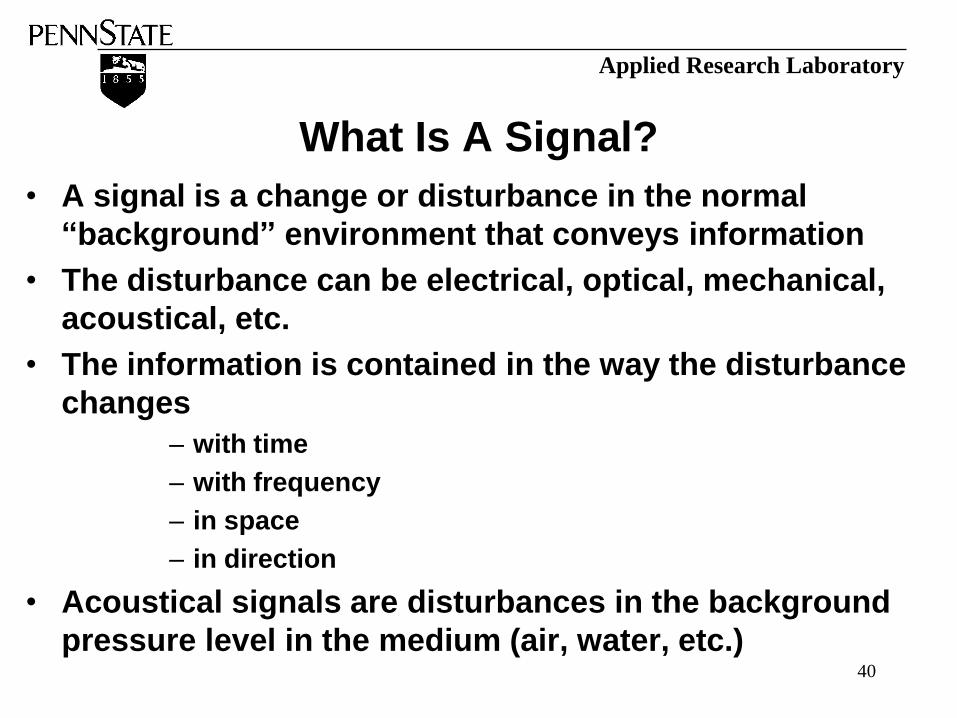
What Is A Signal?

• A signal is a change or disturbance in the normal

“background” environment that conveys information

• The disturbance can be electrical, optical, mechanical,

acoustical, etc.

• The information is contained in the way the disturbance

changes

– with time

– with frequency

– in space

– in direction

• Acoustical signals are disturbances in the background

pressure level in the medium (air, water, etc.) 40


Real and Complex Signals

• A real-valued function of time, f(t), or space, f(x), or both, f(x,t), is

often called a “real signal”.

• It is sometimes useful for purposes of analysis to represent a

signal as a complex valued function of space, time, or both:

• More often, such a function is written in polar form:

• The real-world signal f(t) represented by s(t) is just the real part of

s(t):

)()()( tvituts

(phase) )t(u

)t(varctan)t(

)(magnitude )t(v)t(u)t(R

where

e)t(R)t(s )t(i

22

)t(cos)t(R)t(u)t(s)t(f e

41


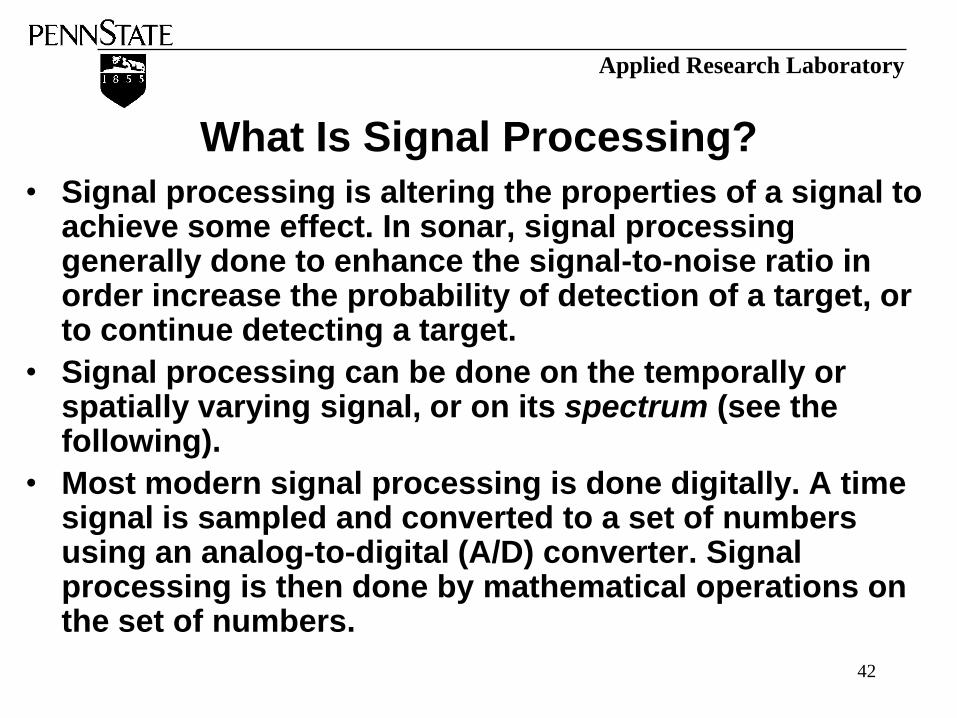
What Is Signal Processing?

• Signal processing is altering the properties of a signal to achieve some effect. In sonar, signal processing generally done to enhance the signal-to-noise ratio in order increase the probability of detection of a target, or to continue detecting a target.

• Signal processing can be done on the temporally or spatially varying signal, or on its spectrum (see the following).

• Most modern signal processing is done digitally. A time signal is sampled and converted to a set of numbers using an analog-to-digital (A/D) converter. Signal processing is then done by mathematical operations on the set of numbers.

42


Spectral (Fourier) Analysis

• Any signal, real or complex, that varies with time can be “broken up into its spectrum” in a way similar to that in which light breaks up into its constituent colors by a prism

• The mathematical operation by which this is accomplished is the Fourier transform

• The Fourier transform of a time signal yields the “frequency content” of a signal

• Much signal processing is done in the “frequency domain” by means of mathematical operations (filters) on the Fourier transforms of the signals of interest

• The result of the processing can be converted back to a filtered time signal by means of the inverse Fourier transform 43


Frequency Domain Signal Processing

• Frequency domain signal processing, or “filtering” alters the frequency spectrum of a time signal to achieve a desired result.

• Examples of filters: band pass, band stop, low pass, high pass, “coloring”,

• Analog filters are electrical devices that work directly on the time signal and shape its spectrum electronically.

• Most filtering nowadays is done digitally. The spectrum of a sampled, digitized time signal is calculated using the Fast Fourier Transform (FFT). The FFT is a sampled version of the signal’s spectrum. Mathematical operations are performed on the sampled spectrum.

• Samples of the filtered signal are recovered using the inverse FFT. 44


Beamforming

45


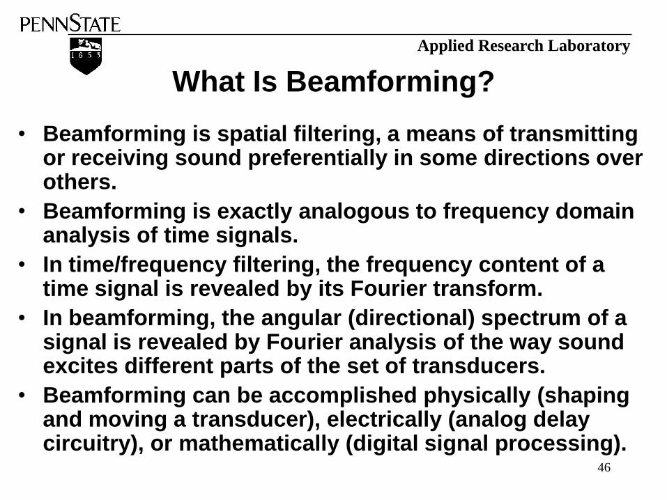
What Is Beamforming?

• Beamforming is spatial filtering, a means of transmitting or receiving sound preferentially in some directions over others.

• Beamforming is exactly analogous to frequency domain analysis of time signals.

• In time/frequency filtering, the frequency content of a time signal is revealed by its Fourier transform.

• In beamforming, the angular (directional) spectrum of a signal is revealed by Fourier analysis of the way sound excites different parts of the set of transducers.

• Beamforming can be accomplished physically (shaping and moving a transducer), electrically (analog delay circuitry), or mathematically (digital signal processing).

46


Beamforming Requirements

• Directivity – A beamformer is a spatial filter and can be used to increase the signal-to-noise ratio by blocking most of the noise outside the directions of interest.

• Side lobe control – No filter is ideal. Must balance main lobe directivity and side lobe levels, which are related.

• Beam steering – A beamformer can be electronically steered, with some degradation in performance.

• Beamformer pattern function is frequency dependent:

– Main lobe narrows with increasing frequency

– For beamformers made of discrete hydrophones, spatial aliasing (“grating lobes”) can occur when the the hydrophones are spaced a wavelength or greater apart.

47


A Simple Beamformer

a

plane wave signal

wave fronts

d

h1

h2

O

plane wave has wavelength

l = c/f,

where f is the frequency

c is the speed of sound h1 h2 are two omnidirectional

hydrophones spaced a distance d

apart about the origin O 48


Analysis of Simple Beamformer

• Given a signal incident at the center O of the array:

• Then the signals at the two hydrophones are:

where

• The pattern function of the dipole is the normalized response of

the dipole as a function of angle:

)t(ie)t(R)t(s

al

sin

d)( n

n 1

a

l

a sin

dcos

s

ss)(b 21

)t(i)t(i

iiee)t(R)t(s

49


Beam Pattern of Simple Beamformer

-150 -100 -50 0 50 100 150 -60

-50

-40

-30

-20

-10

0

a , degrees

Pa

tte

rn L

os

s, d

B

Pattern Loss vs. Angle of Incidence of Plane Wave For Two Element Beamformer, l/2 Element Spacing

0

-10

-20

-30

-40

-50

-180

-165

-150

-135

-120

-105 -90 -75

-60

-45

-30

-15

0

15

30

45

60

75 90 105

120

135

150

165

Polar Plot of Pattern Loss For 2 Element Beamformer

l /2 Element Spacing

50


Beam Pattern of a 10 Element Array

-150 -100 -50 0 50 100 150 -60

-50

-40

-30

-20

-10

0

a , degrees

Patt

ern

Lo

ss, d

B

Pattern Loss vs. Angle of Incidence of Plane Wave For Ten Element Beamformer, l /2 Spacing

0

-10

-20

-30

-40

-50

-165

-150

-135

-120

-105 -90 -75

-60

-45

-30

-15

0

15

30

45

60

75 90 105

120

135

150

165

180

Polar Plot of Pattern Loss For 10 Element Beamformer

l /2 Spacing

51


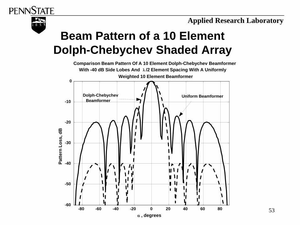
Beamforming – Amplitude Shading

• Amplitude shading is applied as a beamforming

function, usually to the received signal.

• Each hydrophone signal is multiplied by a

“shading weight”

• Effect on beam pattern:

– Used to reduce side lobes

– Results in main lobe broadening

52


Beam Pattern of a 10 Element

Dolph-Chebychev Shaded Array

-80 -60 -40 -20 0 20 40 60 80 -60

-50

-40

-30

-20

-10

0

a , degrees

Pa

tte

rn L

os

s, d

B

Comparison Beam Pattern Of A 10 Element Dolph-Chebychev Beamformer

With -40 dB Side Lobes And l /2 Element Spacing With A Uniformly

Weighted 10 Element Beamformer

Dolph-Chebychev

Beamformer Uniform Beamformer

53


Beamforming – Receive Beam Steering

• To electronically steer a beam to a specific

angle, the hydrophone signals must add so

that a plane wave received at the desired angle

would add in-phase.

• Beam steering implementations:

– Time delay

– Phase shift

54


Beamforming – Transmit

• High power

– Transmit the maximum power on each hydrophone

– Maximum power limited by cavitation

• Desire broad beamwidth for search, narrow

beamwidth for homing

– Desire maximum output power for both types of

transmits -> Generally do not use amplitude shading

on transmit

– Transmit beamforming accomplished by phase

shading of transmit hydrophones

55


Signal Detection

56


Signal Detection

• Input to detector is signal plus noise.

• Requirements expressed in terms of

– probability of detection

– probability of false alarm

• Threshold for declaring detection is set based on

models for signal and noise

• Noise background estimation can be performed on data

to improve model.

• Outputs of detector are threshold crossings

• Performance defined by receiver operating

characteristic (ROC) curve – probability of detection vs.

probability of false alarm for a particular SNR. 57


Detection In Noise

1 2 3

signal

noise mean

noise

signal + noise

noise mean

Time

T2

T1

58


Detection Threshold

• Performance Criteria:

– Probability of detection PD

– Probability of false alarm PFA

• These criteria are not independent: a lower

threshold increases PD, but also increases PFA.

• Theoretical ROC is used to set thresholds.

• True test is performance in water.

59


Receiver Operating Curve (ROC)

T1

T2

Decreasing

threshold

Probability of False Alarm PFA

Pro

bab

ilit

y o

f D

ete

cti

on

PD

0

1

1

60


Noise Background Estimation

• A moving average of the received signal is calculated. This average is used to estimate the background noise level.

• Against noise that changes rapidly with time – e.g. reverberation, noise level must be continually re-estimated for the entire listening interval. -> Use moving average.

• Care must be taken not to average over desired echo, but still get a useful average. Window is usually taken to be the length of the transmitted pulse.

• Higher order statistics can also be estimated this way.

61


Passive Processing

62


Passive Processing Requirements

• Targets:

– Surface ships

– Submarines

– Other sources, e.g. pipeline leaks

• Target Characteristics:

– Broad band

• Level and spectrum dependent on target speed

– Narrow band

• Spectral lines

– Propulsion system

– Propeller cavitation

– Auxiliary machinery

– Spatially compact 63


Target Emissions

Typical ambient noise level

Frequency, kHz

Sp

ec

tru

m L

eve

l (d

B//1

uP

a/H

z @

1m

0.01 1 0.1 10 20

50

70

90

110

150

130

170

190

Submerged submarine, low speed

Large surface vessel, high speed

Some Typical Spectrum Levels

For Surface Ships and Submarines

Frequency

Le

ve

l

Low speed

Broadband and Narrowband Components Of a

Submarine Signature at Low and High Speeds

Frequency

Leve

l

High speed

64


Passive Sonar Requirements

• Target Detection – Passive sonar has an advantage over active for

detection range - less spreading and absorption loss.

• Target Localization – Angle to target

– Precise localization, especially in range and velocity, is more difficult with passive sonar

• Target Characterization – Target signatures help identify target

– Passive sonar won’t mistake a rock for a target

– Active is much more useful for discerning size, shape and structural features 65


Passive Sonar Capabilities

• Beamforming

– Spatial filter

– Increased signal-to-noise – directivity

– Reduces unwanted (out of beam) signals

• Receiver

– Bandpass filter – reduces out of band signals

and noise

– Gain adjust – adjust to receiver circuitry, does

not increase SNR

• Signal processor

• Detector 66


Passive Multibeam

• Increases detection capabilities

– Wide angle coverage

– Directivity of individual beams increase SNR

– Detection processing

• Beam power comparison among beams

• Localization

– Provides bearing to target to within beam

resolution

• Target identification if spectral processing

is used.

67


Passive Narrowband Signal

Processing

• FFT (Spectral Processing)

– Used to detect tones

– Improves detection

– Aids localization by estimating Doppler using

frequency changes in the signal

• Can identify target if its signature is known

68


Passive Short Baseline Localization

• Useful for small sonar arrays

• Technique – offset phase center beams

– Uses the correlation between the inputs of two

subarrays of a beamformer to estimate the angle to

the target.

– The subarrays are closely spaced – 3/2 l or 1/2 l are

often used.

– Useful for enhancing passive detection performance

by allowing fine estimate of angle to detection.

69


Passive Long Baseline Localization

• Useful for arrays of widely spaced hydrophones

• Technique – Correlation processing with variable time shift – Time shift with highest correlation gives time

delay for reception between each hydrophone.

– Useful for enhancing passive detection performance.

– Can be used to estimate angle to target. Multiple hydrophones (3 or more) can be used to triangulate.

70


Active Processing

71


Active Sonar Requirements

• Target Detection

• Target Localization

– Range

– Angle

– Doppler -> line-of-sight velocity

• Target Characterization

– Size

– Shape

– Orientation

– Finer details 72


Typical Active Beamformer Configurations

• Transmit

– Wide angle – search volume coverage

– Narrow angle – homing

– Source level increases as beam narrows

• Receive

– Search – Multiple narrow beams for high directivity

– Homing – Narrow detection beam with offset phase

beams

73


Active Sonar Beamsets

15

-30 30

-15

Az

El

Az

El

Az

El

3 dB Beamformer Contours

Search Long Range Homing Close-In Homing

Az

El

Transmit

Receive Az

El

Az

El

74


Target Properties

• After accounting for propagation losses, the

target echo level is proportional to the

transmitted source level

• The proportionality “constant” is the target

strength

– Depends on sound reflecting properties of the target

– Function of frequency, signal resolution, and aspect

angle

– Target highlights (echoes from reflecting surfaces)

add with random phase.

75


Variation of Target Strength

15

20

Bow

Stern

10

5 Beam

Typical submarine target strength

in dB as a function of aspect angle

Notes:

• TS is a function of frequency

• Graph at right is more representative

of a low frequency

• High frequency graph of TS would

have similar rough shape, but would

have significantly more detail

• “Spikier” due to higher resolution

of target features 76


Target Echo and Signal Resolution

tp

Pulse width matched to target length

Time

tp 2L/c

2L/c

2L/c + tp

tp << 2L/c

Pulse width small compared to target length

77


Effect of Motion on Echo

• For stationary sonar and target: – Echo spectrum Signal spectrum

• For moving sonar or target, spectrum of echo is shifted and spread.

• Shift is “Doppler shift”. Doppler shift is due to: – Target motion

– Sonar motion

• Doppler shift due to sonar motion can be somewhat negated by shifting the transmit or receive frequency to account for sonar motion – own-Doppler nullification (ODN).

• Spectral spreading is due to numerous factors, in particular the fact that different parts of the target move with different speeds relative to line-of-sight vector.

78


Effect of Reverberation

• For stationary conditions (“quiet sea”):

– Reverberation spectrum Signal spectrum

• Spectrum of reverberation is more generally

shifted and spread.

• Spectral shift and spreading is due to:

– Scatterer motion

• Surface reverb scatterer motion dependent on sea state

• Volume reverb scatter motion depends, e.g., on presence of

fish, suspended bubbles or solid material, currents, etc.

– Sonar motion

• Off-axis scattering

79


Active Detection Processing

• One of the most common active detectors is the

matched filter.

– Peak output SNR is optimized against additive white

Gaussian noise with a matched filter.

• Can be implemented by correlating received signal with

replica of transmitted signal at varying time shifts.

– Time shift with peak output above threshold yields target

range,

• To account for frequency (Doppler) shift in received

signal due to target motion, the detector is usually

implemented in the frequency domain – frequency

shifted detections can be located on “Range-Doppler

map. 80


Matched Filter Implementation

Time/Range

Received signal time series

Replica correlate

& FFT each slice

Time slices

Time/Range

Frequency

or Doppler

Frequency slices

Range-Doppler Map 81


Range-Doppler Maps

• A Range-Doppler map is a representation of the

power spectral level of an acoustic echo as a

function of time.

• The time axis is usually converted to range,

while the frequency axis is converted to

equivalent Doppler shift.

• The resulting surface is reduced to a two

dimensional plot for presentation using colors to

represent level.

• The levels in each Range-Doppler cell can be

processed to find detections. 82


Effect of Reverberation (Continued)

• Reverberation is an echo of the transmitted signal.

• When ODN is used, the reverberation spectrum is

centered at about the transmit frequency (zero frequency

when basebanded).

• The spectrum continues as long as the reverberation can

be detected. (“Reverb ridge”)

• Even though target echo level falls off faster than

reverberation with range, targets off of the reverb ridge

(high Doppler targets) can be detected at long range.

• Signal design for low Doppler targets attempts to

mitigate effects of reverb ridge.

83


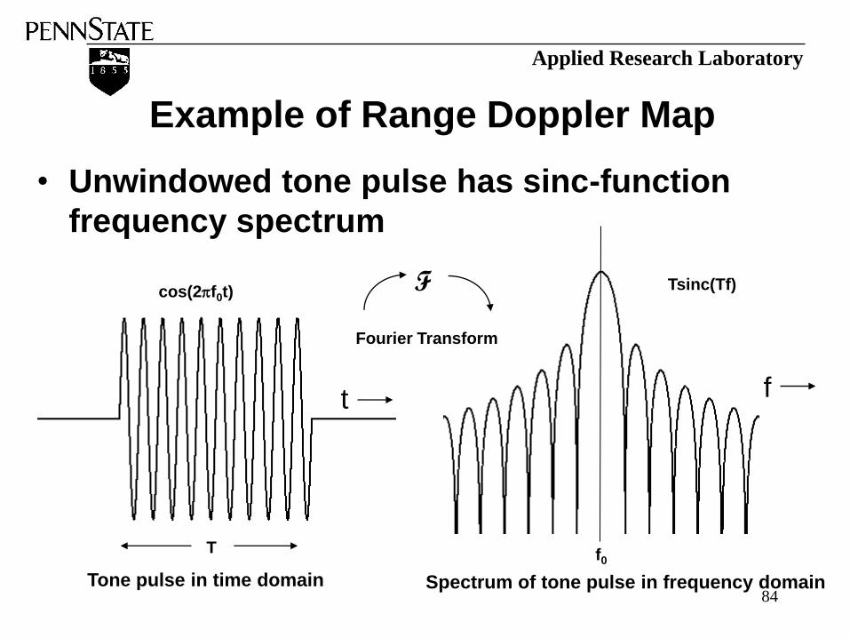
Example of Range Doppler Map

• Unwindowed tone pulse has sinc-function

frequency spectrum

t f

Tone pulse in time domain Spectrum of tone pulse in frequency domain

F

Fourier Transform

cos(2f0t)

T

Tsinc(Tf)

f0

84


Reverberation ridge

Target detection:

Would not have been

detected if it had been

moving slower.

High sidelobes

of unwindowed tone pulse

Basebanding and ODN

shifts spectrum to 0 Hz and

eliminates sonar’s motion

Example Of A Range-Doppler Map (Volume Reverberation, Stationary Sonar)

85


Signal Selection

• Range resolution is inversely proportional to

signal bandwidth.

– For tone pulses, this translates to range resolution is

proportional to pulse length:

• Pulse bandwidth is inversely proportional to tone pulse

duration, so

• Short pulses => Short (“high”) range resolution

– For linear FM sweeps, range resolution is inversely

proportional to width of sweep.

• Wide frequency sweep => Short (“high”) range resolution

• Doppler resolution is inversely proportional to

pulse length. • Short pulse duration => Wide (“low”) Doppler resolution 86


High Doppler Targets

• Tone pulses can be good choices for high Doppler targets: – Target is out of the reverberation ridge

– Longer pulses used for detection have excellent Doppler resolution

– Short pulses used for close-in homing have excellent range resolution.

• Drawbacks: – Targets that are changing aspect can be lost in

reverberation ridge

– As sonar closes in on target, short pulses are used. Reverberation spectrum is very wide for short pulses. Can loose even high Doppler targets 87


Low Doppler Targets

• Processing gains can be attained against low

Doppler targets by using linear sweep FM

pulses.

• Advantages: spreads (and hence lowers)

reverberation power over bandwidth of

frequency sweep, but coherently processes

echo => Processing gain ~ 10·log(TW), where T

is pulse length and W is signal bandwidth

• Drawbacks:

– Increasing T to increase PG is not viable when target

is very close or target position is changing rapidly.

But short T means less Doppler resolution. 88

Sonar Implementation Concepts - Pennsylvania State … Implementation ... –signal detection ......

Documents

Transcript of Sonar Implementation Concepts - Pennsylvania State … Implementation ... –signal detection ......