Some Unintended Fallout from Defense Policy: … Unintended Fallout from Defense Policy: Measuring...

Some Unintended Fallout from Defense Policy:

Measuring the Effect of Atmospheric Nuclear Testing on

American Mortality Patterns

Keith Meyers

University of Arizona ∗

Current Version

October 24, 2017

Abstract

During the Cold War the United States detonated hundreds of atomic weapons at the

Nevada Test Site. Many of these nuclear tests were conducted above ground and released

tremendous amounts of radioactive pollution into the environment. This paper combines

a novel dataset measuring annual county level fallout patterns for the continental U.S.

with vital statistics records. I find that fallout from nuclear testing led to persistent

and substantial increases in overall mortality for large portions of the country. The

cumulative number of excess deaths attributable to these tests is comparable to the

bombings of Hiroshima and Nagasaki.

JEL Codes: I10; N32; Q50. Keywords: Nuclear Testing, Public Health, Radioactive

Fallout, Defense Policy

∗Meyers, Keith. 1000 E Water Street #5, Tucson, AZ 85719; Economics Dept. Fax: 520.621.8450, Phone:937-570-0782; Email: [email protected]. Manuscript word count: 8,440. This material is basedin part upon work supported by the National Science Foundation under Grant Number SES 1658749. Anyopinions, findings, and conclusions or recommendations expressed in this material are those of the author(s)and do not necessarily reflect the views of the National Science Foundation. Thanks to Price Fishback, DerekLemoine, Ashley Langer, Joesph Ferrie, Jessamyn Schaller, Gary Solon, and Cihan Artunc for feedback, dataand support. Additional thanks to Andre Bouville, Steven Simon and the National Cancer Institute for theirhelp providing fallout deposition records.

1

https://keith-meyers.squarespace.com/s/MeyersFalloutMortalityWebsite.pdf

Pollution is often the byproduct of human activity and imposes significant costs upon the

public. In many settings, the government attempts to address the external costs associated

with polluting activities, but there are cases where government policy is the direct cause of

harmful pollution. During the Cold War the United States detonated hundreds of nuclear

weapons just northwest of Las Vegas at the Nevada Test Site (NTS). Prior to 1963 many of

these tests were conducted above ground and released tremendous quantities of radioactive

material into the environment. One estimate places the total atmospheric release of radioac-

tive material from the NTS as over 12 Billion Curies between 1951 and 1963. In comparison,

Chernobyl released an estimated 81 Million Curies of radioactive material (LeBaron, 1998).

These nuclear tests exposed millions of Americans to harmful radioactive material and many

people are still living with the consequences of this pollution today. This paper measures

the effect of domestic atmospheric nuclear testing on the crude death rate for the entire

continental United States. I present evidence that nuclear testing had broad and adverse

effects on human capital in the extreme and contributed to at least as many deaths as the

bombings of Hiroshima and Nagasaki.

The medical and scientific literature studying the health effects of nuclear testing has

focused primarily upon small samples of populations who lived in the areas surrounding

the Nevada Test Site.1 These studies examine the health effects of fallout exposure in these

populations and extrapolate out the potential health consequences for the nation. Simon and

Bouville (2015) of the National Cancer Institute (NCI) note that there is great uncertainly

underlying these estimates. They estimate that fallout from domestic nuclear testing caused

49,000 thyroid cancer deaths.2 One of the major drawbacks of these medical and scientific

studies is that they fail to capture the temporal and geographic scope of these health effects.

1The region surrounding the NTS is termed Downwind in the literature and this area consists of the fewcounties in AZ, NV, and UT surrounding the test sight.

2The 95 percent confidence interval for this estimate is 11,300 and 220,000 deaths. Simon and Bouville(2015) suggest testing contributed up to 11,1000 additional of other cancer deaths. Without nuclear testingthey estimated that 400,000 cases of thyroid cancer would arise naturally in the same population.

2

Using an alternative empirical approach, this paper provides substantial evidence that

nuclear testing had profound effects on American health. I combine measures of radioactive

fallout exposure from National Cancer Institute (1997) and mortality data for the continental

U.S. to analyze the mortality effects of atmospheric nuclear testing. By using within county

variation in fallout deposition across years, this paper measures both the geographic and

temporal extent of the harm caused by nuclear testing. The results from the empirical

analysis reveal that nuclear testing led to prolonged increases in the crude death rate in

many regions of the country. Contrary to the assumptions made in the medical literature,

the largest mortality effects occurred in the Great Plains and Central Northwest U.S., far

outside of the areas studied by the current literature. Back-of-the-envelope estimates suggest

that fallout from nuclear testing contributed between 340,000 to 460,000 excess deaths from

1951 to 1973.

Economists have extensively studied the effects of air pollution, lead contamination, and

other pollutants upon mortality and public health, but little economic research has stud-

ied the public health consequences of atmospheric nuclear testing.3 The economic research

studying the social costs and consequences of radioactive pollution has focused primarily

on Scandinavian and Ukrainian populations. Danzer and Danzer (2016) and Lehmann and

Wadsworth (2011) study the cost of the Chernobyl disaster to Ukrainian populations us-

ing cross sectional variation in exposure. Another body of research has successfully used

variation in multiple sources of air pollution as a shock to test the fetal origins hypothesis

(Almond et al., 2009a; Almond and Currie, 2011; Currie, 2013; Currie et al., 2015; Isen et al.,

2017). With respect to radioactive pollution, both Almond et al. (2009b) and Black et al.

(2013) use radioactive pollution to test the fetal origins hypothesis in Scandinavia. Almond

3 Work by Hanlon (2015) has shown that coal consumption in 19th Century England had substantial effectson mortality rates and that coal utilization. Barreca et al. (2014) and Clay et al. (2016) study the long-termhealth consequences of using coal for heating and electricity generation for the United States. Troesken (2008)and Clay et al. (2014) study how historic municipal decisions relating to the adoption of lead water pipes hadlong run effects on public health.

3

et al. (2009b) use radioactive fallout from the Chernobyl disaster and associate negative ed-

ucational outcomes with in-utero exposure to fallout in Swedish cohorts. Black et al. (2013)

use data from 14 radiation monitoring stations in Norway to study exposure in cohorts born

between 1956 and 1966. They discover persistent and statistically reductions in educational

attainment, earnings, and IQ scores among cohorts exposed during months three and four

of gestation.

The results of this paper corroborate the negative effects found in previous research and

improves upon the identification by exploiting the specific biological mechanisms through

which American populations were exposed to harmful radioactive toxins. Radioactive fall-

out deposition can be an imprecise measure of human exposure to harmful ionizing radi-

ation. Humans only metabolize specific radioactive isotopes created through fission. The

primary mechanism through which people were exposed to concentrated doses of radiation

was through the ingestion irradiated food products. Fallout deposition may approximate the

presence of fallout in the local food supply, but radiation exposure proxied through deposition

becomes more inaccurate if local deposition fails to enter the local food supply. The National

Cancer Institute (1997) finds that the consumption of irradiated dairy products served as

the primary vector through which Americans ingested large concentrations of radioactive

material. During the 1950’s most milk was consumed in the local area it was produced.

It is through this channel where local fallout deposition would enter the local food supply

(National Cancer Institute, 1997). This paper leverages estimates of I-131 concentrations in

locally produced milk to provide a more precise estimate of human exposure to fallout than

previous studies.

4

1 Medical, Scientific, and Historical Background

1.1 History of NTS

In the 1950’s, millions of Americans were unknowingly exposed to radioactive fallout

through both the environment and the food supply. With respect to economic and de-

mographic activities, exposure to radioactive matter from atmospheric nuclear testing can

generally be considered as a plausibly exogenous event. Radioactive pollution is often an

invisible and imperceptible threat to human health. National security concerns in the 1950’s

motivated atomic testing at the NTS. While the location of the base was not random, the

base was not chosen due to surrounding characteristics of the residing population.4

Atmospheric atomic testing on U.S. soil was a deliberate policy decision made by do-

mestic political leaders. In 1949 the Soviet Union detonated its first nuclear bomb Joe-1.

Provoked and surprised by this sudden event, U.S. political and military leaders sought to

accelerate America’s own nuclear weapons program. Prior to this event, nuclear testing oc-

curred in the Pacific.5 The Pacific tests proved logistically costly, slow to implement, and

expensive. American leaders sought a convenient testing location and settled on the Nevada

Test Site due to its proximity to U.S. government labs, low levels of precipitation, and rela-

tively secluded location (Center for Disease Control, 2006; National Cancer Institute, 1997).

Located in Nye County, Nevada, this military zone became the epicenter of the American

nuclear weapons program. Nuclear testing occurred from 1951 until 1992. The period of

atmospheric nuclear testing occurring between 1951 and 1963. During this period, the U.S.

detonated 100 atmospheric bombs at the NTS (US Department of Energy, 2000).

4The base was chosen over more environmentally friendly locations due to its proximity to governmentlabs, access to public land, and rapid ease of establishment (Schwartz, 2011).

5The three Trinity test in 1945 were conducted in White Plains New Mexico. All other tests conductedprior to the opening of the NTS occurred in the Pacific.

5

During the 1950’s, the public was largely unaware of the dangers that the NTS posed

to public health. Often, the Public Health Service (PHS) and Atomic Energy Commission

(AEC) sought to dismiss fears regarding the atomic testing. Official government statements

made during the testing period asserted that all dangerous radioactive material remained

within the confines of the NTS.6 At best, these organizations failed to adequately warn

civilians living around the test site of the health risks associated with these atomic tests

(Ball, 1986; Fradkin, 2004; LeBaron, 1998). In 1978, the plight of populations living near

the NTS received national media attention. Subsequent Freedom of Information Act requests

later revealed that the government knew of these dangers to public health the NTS tests posed

and that the AEC had suppressed medical studies highlighting the health dangers (Fradkin,

2004).

1.2 The Health Consequences of Radiation Exposure

Radioactivity generally refers to dangerous particles given off by radioactive decay of

matter. The weakest forms of ionizing radiation are alpha particles, and these particles

generally cannot penetrate most thin physical barriers. Beta radiation is more dangerous

and can penetrate deep into flesh and cause damage. Gamma radiation is the most dangerous

form of radioactivity and consists of highly energetic photons. Gamma radiation can travel

easily through the body and causes immense damage to biological tissues.

With regards to nuclear testing, there are three radioactive isotopes of concern to human

health because of their relative radioactivity, prevalence, and how they are metabolized.

These isotopes are Iodine-131, Strontium-90, and Cesium-137. Other isotopes created during

nuclear fission are less dangerous to human health because they do not remain in the body for

6In the Appendix is an example of a 1951 AEC flyer explicitly iterating this official claim. Thewebsite for the Official Department of Energy Nuclear Testing Archive where this flyer is from ishttps://www.nnss.gov/pages/resources/NuclearTestingArchive.html. The government circulated flyers suchas these in the areas surrounding the NTS, all while the AEC and PHS detected substantial quantities offallout depositing in populated areas far beyond the confines of the atomic test range.

6

extended periods or because they are created in minuscule quantities. Many other radioactive

isotopes pass through the body and are secreted following ingestion. In particular, Iodine

131 is a potent radioactive poison. It possesses an eight day half-life, concentrates in the

thyroid gland, and emits highly active forms of beta and gamma radiation as it decays

(LeBaron, 1998). These traits of I-131 cause acute and rapid damage to tissue surrounding

the thyroid. Strontium 90 also appears in wheat and plant products in limited quantities.

This isotope collects in bones and teeth. It decays over a long period and causes prolonged

damage. Sr-90 possesses a 25 year half-life, diffuses across the body uniformly and emits beta

radiation (LeBaron, 1998). Finally, Cs-137, which was released in large quantities during the

recent Fukushima Daiichi disaster, collects in fleshy tissue and does not concentrate in any

particular organ. It has a half-life of 33 years and emits both alpha and beta radiation

(LeBaron, 1998).

The medical and scientific knowledge regarding the effects of human exposure to ionizing

radiation comes from many sources. Studies of Japanese atomic bomb survivors and persons

living downwind of nuclear test sites provide much of this knowledge. In human population

studies of radiation exposure, researchers have measured a variety of negative health and

developmental consequences from exposure to ionizing radiation. Studies of atomic bomb

survivors and persons exposed during pregnancy demonstrate increased cancer risks, nega-

tive developmental and cognitive effects due to radiation exposure (Lee, 1999; Otake et al.,

1993; Otake, 1996; Schull, 1997). Researchers studying Chernobyl have found greater inci-

dences of thyroid cancers, and lesions indicative of I-131 poisoning in exposed population

(Shibata et al., 2001; Williams, 2002). Researchers studying downwind American popula-

tions have also found evidence of increased thyroid cancer and leukemia risks in domestic

downwind cohorts (Gilbert et al., 2010; Kerber et al., 1993; Stevens et al., 1990). Together,

the medical and scientific literature suggest that exposure to ionizing radiation increases the

7

risks of various types of cancer and can have detrimental effects upon human growth and

development. An additional effect of fallout exposure is that it could degrade health, inhibit

immune responses, and cause people to die from other non-cancer related causes.

1.3 Exposure Mechanisms

Exposure to harmful radioactive fallout can occur either through direct channels or indirect

channels. Radioactive material can enter the body if it lands on the skin with radioactive

dust. Many people and animals living in the downwind counties surrounding the NTS were

exposed to harmful fallout in this matter. People can inhale radioactive material when

it is suspended in the air. Inhalation of radioactive dust would be the most likely in the

downwind region. Research by the National Cancer Institute (1997) and Center for Disease

Control (2006) establishes that the food supply served as the main indirect vector of exposure

for most Americans during the atomic testing period. Scientific evidence contemporaneous

with the testing period also substantiates that radioactive materials resulting from nuclear

fission appeared in crops, people, and animals (Beierwaltes et al., 1960; Garner, 1963; Kulp

et al., 1958; Olson, 1962; Van Middlesworth, 1956). Similarly, the PHS also released research

corroborating this evidence but downplayed the health risks associated with the radiation

levels reported (Flemming, 1959, 1960; Wolff, 1957, 1959). These government studies often

downplayed the risk associated with the levels of radioactive material found in independent

studies as alarmist.

The NCI establishes the dairy channel as a primary vector through which Americans

were exposed to significant quantities of radioactive material. Most Americans would not

be exposed to radioactive dust carried by low altitude winds. Instead, high altitude winds

would carry the material far from the test site and the material would only deposit on the

ground if it happened to be precipitating while the radiation cloud was overhead. In the few

days following the nuclear test, this radioactive material would deposit on crops and pasture.

8

Some radioactive material would enter wheat and other plant products, but consumption of

these products would not necessarily be in the same region where they were produced. Dairy,

however, during the 1950s and 1960s was generally produced and consumed locally (National

Cancer Institute, 1997). During the 1950s most milk was produced near population centers

and delivered daily. In the late 1950s refrigerated truck adoption spread and deliveries

switched to every few days (Dreicer et al., 1990). The dairy channel is unique in that cows

would consume large quantities of irradiated pasture and concentrate radioactive material,

specifically I-131, in milk.

People living in the region where deposition occurred would then be more likely to consume

this irradiated food product containing a potent radioactive poison in the days following the

atomic test. Pasturing practices would affect the quantities of fallout entering the dairy

supply. The areas surrounding the NTS experienced the greatest quantities of radioactive

fallout deposition, but often had very little I-131 entering the dairy supply. Dairy farming

practices in much of AZ, NV, and UT in the 1950s relied on importing hay from outside

regions and as such very little radioactive matter would enter the food supply. This in turn

makes deposition itself a less accurate proxy for human exposure to fallout in these areas.

2 Empirical Strategy: Measuring Short Term and Long Term

Mortality Effects

2.1 Empirical Model

The empirical analysis of this paper focuses on two different panel regression models to

ascertain the geographic and temporal extent of the health cost of atomic testing. The first

set of regressions test whether within county variation in radioactive fallout exposure across

years had an immediate effect upon crude death rates using a distributed lag framework.

9

Short run changes in the crude death rate from fallout exposure are potentially less vulnerable

to measurement error in treatment and migration bias than regressions measuring the long

run effects of fallout. These regressions, however do not fully capture the temporal extent of

these increases in mortality rates. The negative health effects of radiation poisoning often

materialize long after the damage has occurred. A set of long run regressions employ a

distributed lagged framework and pool exposure into five year averages. Estimation of this

model measures how persistent the effects of fallout were on crude death rates, accounts

for the cumulative effect of fallout exposure over multiple years, and whether exposure to

fallout led to harvesting. If exposure to radioactive fallout shortened lifespans and exposed

populations who died tended to die at younger ages than if they were not exposed, then

these people would not appear in subsequent years in the county panel. This harvesting

effect would decrease estimated mortality rates many years following the initial exposure

event, because people who would have died in these periods died earlier in the sample.

yit = Σ5k=0βk ∗Xit−k + αi + γst + εit (1)

Equation (1) describes the full model specification of this paper. This model tests whether

radioactive fallout in locally produced milk or in the environment had a statistically sig-

nificant effect upon mortality in the years directly following the test. The outcome de-

noted by yit measures the number of total deaths per 10,000 people in a given county i

and year t. Xit−k denotes the exposure variable used to proxy for fallout exposure. There

are two different measures of radiation exposure used in the analysis. These measures are

ground deposition of I-131 and I-131 concentrations on locally produced milk. The variable

Deposition Exposureit denotes the cumulative measure of total radioactive iodine deposited

per square meter in each county year.7

7Alternative functional forms find similar results. These alternative specifications are reported in theonline appendix.

10

The variable Milk Exposureit denotes the measure of radioactive iodine in locally pro-

duced milk in each county year in thousands of nCi per day/Liter. The NCI created daily

integrated estimates of secreted iodine per liter of milk for each nuclear test. They then

summed up these secretions over the entire test series. If a cow in a county produced one

liter of milk each day, this would measure the amount of radioactive iodine secreted in all

those liters of milk in each year. Furthermore, the milk variable accounts for grazing practices

across regions. Cows in upstate New York would not have been exposed to much radiation

from February tests as they would have been inside barns consuming fodder while cows in

Georgia or Texas would have been exposed.

The variables αi and γst denote county and state-by-year fixed effects. These county fixed

effects control for time invariant county characteristics. The state-by-year fixed effects ac-

count for unobserved annual shocks shared across counties within the same state and year.

One drawback of state-by-year fixed effects is that they might control for much of the effect

of radioactive fallout exposure. Only variation in fallout exposure between counties within

the same state provide identification.8 Alternative specifications replace these state-by-year

fixed effects with year fixed effects and state specific time trends to control for possible un-

derlying trends in the data that might be correlated with the exogenous variable of interest.

The variable εit denotes the heteroskedastic error term and is clustered at the county level.9

yit = Σ5j=0θj ∗Avg Xit,j + αi + γst + εit (2)

8 Only variation in county level exposure above or below the state year average for exposure providesidentification. It is quite likely that the effect of fallout exposure will be underestimated when using state-by-year fixed effects, since the identifying variation is narrower.

9Multiple yearly lag structures were tried and the results are generally robust with respect to the numberof lags. A specification with five lags was selected since the long run specifications use five year averages.Using five year lags identifies the mortality effect of fallout exposure that is being averaged in the long runpanel.

11

Equation (2) describes the distributed lag specification for the long run panel regressions.

This model uses a similar framework to that of Equation 1, but the exposure of interest

consists of lagged five year averages of the I-131 exposure measures. The variable Avg Xit,j

denotes the average exposure term with j lags. This distributed lag structure measures the

dynamic mortality response to county level radiation exposure over a longer time horizon.

Fallout in the current year is excluded from the regression and only past deposition patterns

provide variation. This model uses variation in average fallout exposure one to five years

prior, six to ten years prior, eleven to fifteen years prior, sixteen to twenty years prior, and

twenty-one to twenty-five years prior to identify the temporal extent to which fallout affected

mortality patterns.

2.2 Identification and Sample

The source of identifying variation in the empirical analysis comes from within county

variation in radiation exposure across years after controlling for state specific annual shocks.

There are two main assumptions that allow for measurement of the causal effect of fallout

upon mortality. The first assumption is that the exposure variable is orthogonal to the

unobserved error term. The second assumption is that most people who were exposed to

radioactive fallout eventually die in the county where they were exposed.

Fallout exposure from nuclear testing is a plausibly exogenous event. First, the public gen-

erally cannot observe whether they are exposed to radioactive pollution. Radioactive threats

generally are imperceptible. Second, the public generally did not know about the polluting

effects of the NTS until long after atmospheric testing was suspended. The imprecise pub-

lic knowledge regarding the effects of fallout exposure prior to 1978 suggests such behavior

would be unlikely for much of the country. One challenge to the orthogonality assumption is

that people living in the counties surrounding the NTS could observe radioactive dust blows

from atomic tests and might have engaged in avoidance behaviors. In order to avoid these

12

potential endogeneity issues, I exclude the counties surrounding the NTS and those counties

listed as Downwind by the US Department of Justice (2016) from the empirical analysis.10

Outside of these counties, people would have been exposed to fallout through the irradiated

food supply and not by visible radioactive dust blows.

The second assumption is necessary to measure the treatment effect of fallout upon mortal-

ity patterns. Since exposure is at the county level rather than individual level, identification

relies on people dying in the counties where exposure is reported. In and out migration

would introduce measurement error in the treatment variable. If migration decisions are

not systematically correlated with radiation exposure, then migration bias should attenuate

the effect of radiation exposure on mortality as the time between the exposure event and

reported deaths widen.

2.3 Public Health Data

The empirical analysis uses a county-level annual panel constructed by Bailey et al. (2016)

of crude deaths from 1915 to 2007 from Annual Reports of the U.S. Vital Statistics. A

subsample from 1940 to 1988 forms the panel for the bulk of the empirical analysis and

is selected for its completeness of county level coverage. This panel is used to measure the

geographic and temporal extent to which radioactive pollution from the NTS harmed human

health. The crude death rate per 10,000 individuals approximates the total mortality effect

associated with fallout exposure. Exposure to ionizing radiation can increase cancer risks,

but exposure might also make persons less healthy overall and increase non-cancer related

mortality rates.

10A total of 26 counties are excluded from the analysis. These counties are all located in AZ, CA, NV, andUT. Relatively speaking, very few individuals resided in these counties during the testing period and theseareas experienced large quantities of fallout deposition. Including these counties into the sample does notsubstantially affect the estimates using milk exposure but substantially affects the precision of the depositionmeasures. Including an interaction term for these counties or taking the log of the treatment variable correctsfor the imprecision these counties introduce for the deposition measure.

13

2.4 Fallout Exposure Data

In 1983, Congress authorized the Secretary of Health and Human Services to investigate

and measure thyroid doses from I-131 in American citizens. The NCI undertook the task of

gathering radiation monitoring station data from historical records. With these records and

weather station data the NCI could track the position of the radiation cloud, determine how

much radiation would deposit with precipitation, and employ kriging techniques to estimate

fallout deposition in counties without monitoring stations. Much of the raw data came

from national monitoring stations whose number varied across time, but never exceeded

100 stations. The military also engaged in air monitoring and used city-county stations

around the NTS to track the radiation cloud National Cancer Institute (1997).11 These are

the most complete and comprehensive measures for fallout deposition from nuclear tests for

the United States. The data employed in this paper are derived from the NCI estimates.

The NCI provides estimate for I-131 deposition for each nuclear test conducted from 1951

to 1958, except for three tests in the Ranger 1951 series.12 The depositions are measured

as nanoCuries (nCi) per meter squared and are reported for each day following a nuclear

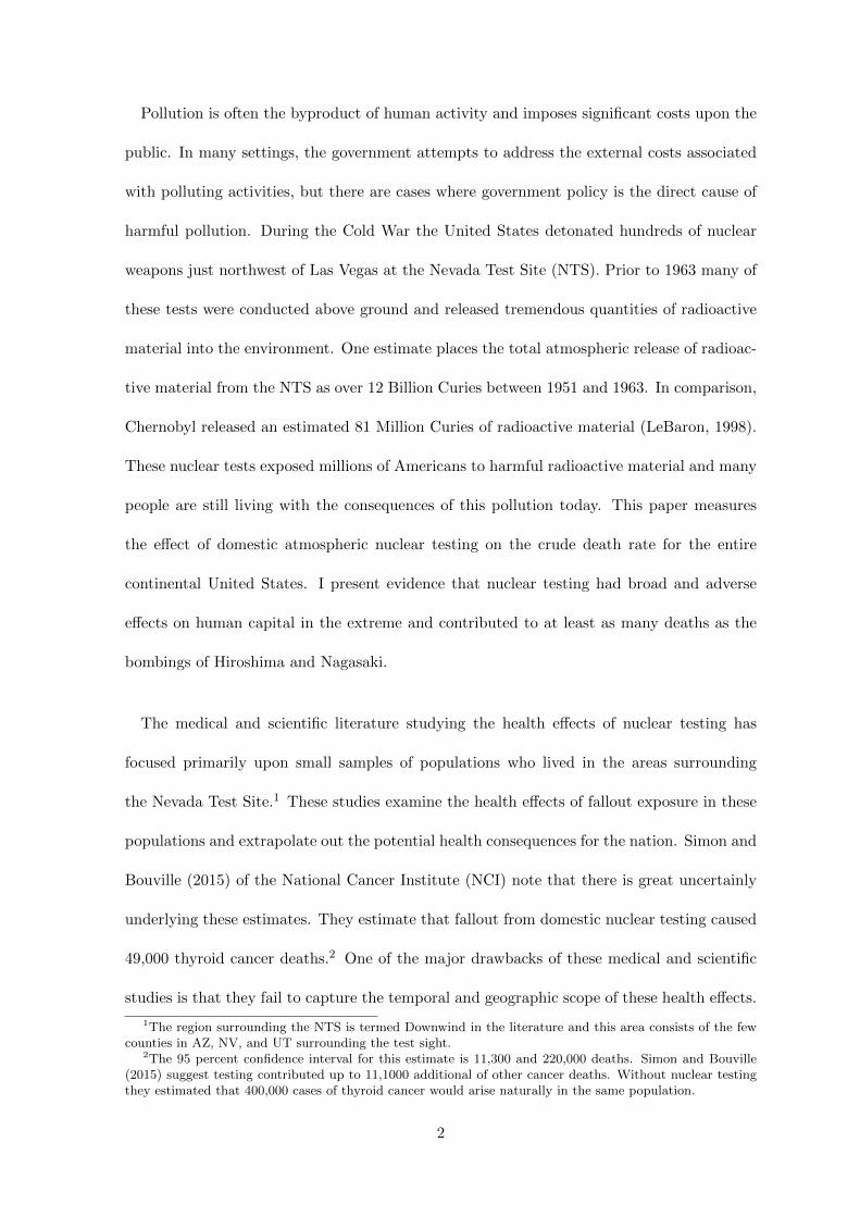
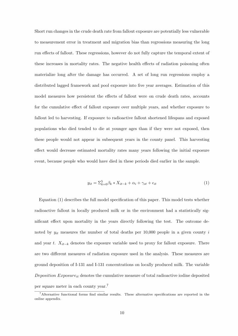
test until the next subsequent test in the series. Figure 1 provides a map of my deposition

data for the Upshot Knothole test series. This map show how geographically extensive and

heterogeneous fallout patterns are across the country. Notice how states such as Vermont

and New Jersey experienced large depositions in 1953.

The NCI also provides daily integrated estimates for I-131 secreted in locally produced

milk. These measures are a function of how cows metabolize and secrete iodine at different

levels of exposure, grazing practices during the testing window, and the levels of radiation de-

position estimated in the kriging model. This methodology can cause substantial differences

11The locations of monitoring stations is not available through National Cancer Institute records.12The National Cancer Institute is currently trying to create estimates for deposition using simulation

methods since monitoring station data is missing for the first three Ranger tests. These tests are not includedin this paper’s analysis.

14

between radiation presence in milk estimated at the county level and deposition. During the

1950’s, many households consumed locally produced dairy, and I-131’s short eight-day half-

life means that persons would consume it before the radioactive I-131 would decay. Children

would be especially vulnerable to this radiation exposure channel because they tended to

drink more milk than adults, had smaller thyroids, and were still growing during this period

(National Cancer Institute, 1997). Since a child’s thyroid is smaller than an adult’s, the

same quantity of I-131 would cause greater damage because it would be concentrated into

a smaller area. Furthermore, the thyroid regulates growth and development. Harm to this

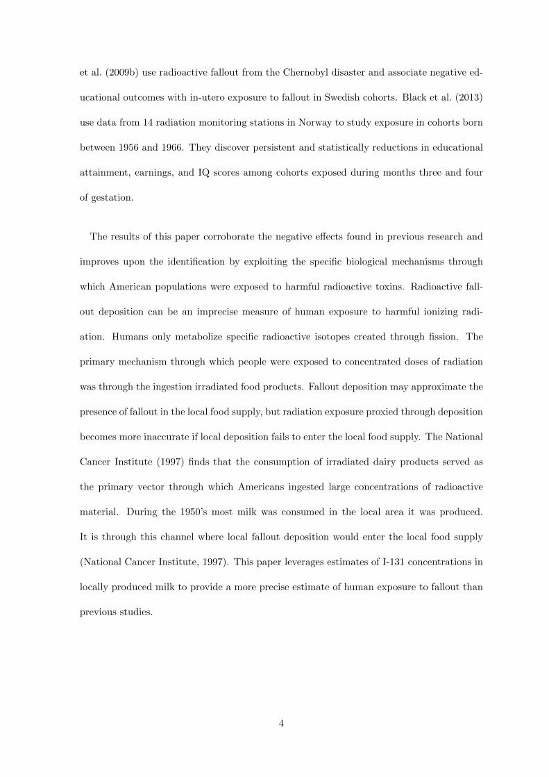
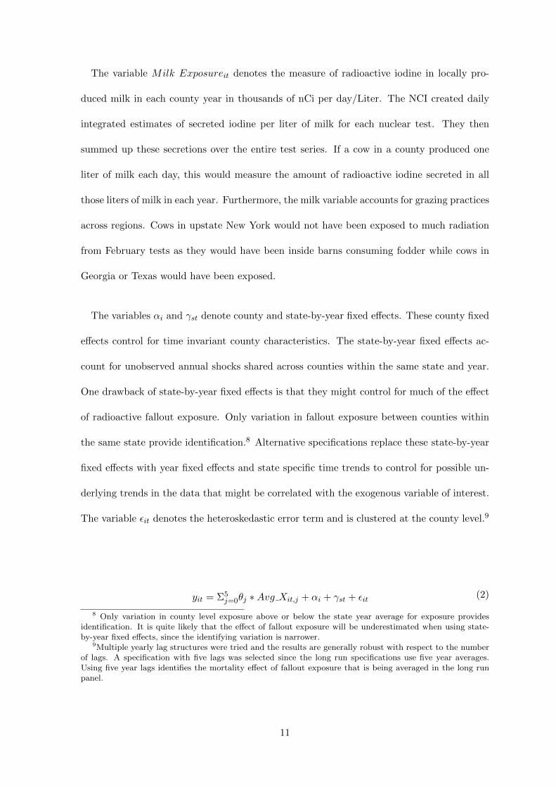
organ might lead to unanticipated long term health problems. Figure 2 provides a map of

my milk exposure data for the Upshot Knothole test series.13 Notice how milk measures vary

from the deposition measures. Areas with the highest levels of ground deposition around the

NTS have relatively low levels of I-131 present in the local milk supply.

The counties downwind of the NTS experienced fallout mostly as dry precipitate, and

according to the agronomic data provided by the NCI, dairy cows in these areas consumed

very little local pasture. This can create a substantial difference in the estimated exposure

via milk versus estimated exposure via deposition.

ICMpij =

∫ ∞0

Cp(ijt) ∗ P (ijt) ∗ fmdt (3)

Equation (3) refers to the NCI’s methodology for estimating daily I-131 concentrations

in milk from deposition data. ICMpij denotes the Integrated I-131 concentration in milk

produced in pasture p in county i on day j and is measured in daily nCI per liter of milk.

Cp(ijt) denotes average daily concentration after deposition day. It is a function of deposition

of I-131 and the fraction of this I-131 intercepted by plants. P (ijt) denotes the average

13A small number of counties in both the deposition and milk measures consistent of sub county units. Icreated weighted averages of exposure at the county level from these subcounty units. In the analysis, thesecounties are excluded from the main sample. Other counties and Virginia Independent Cities are omittedfrom the sample due to data limitations.

15

pasture consumption rate by cows and was constructed from agronomic studies relating to

pasturing behavior of dairy farmers during the 1950’s. The value fm denotes I-131 intake

to milk transfer coefficient. This value was constructed from milk secretion studies where

cows were fed radioactive iodine. These adjustments are made at the state level and should

not be systematically correlated with any unobserved underlying economic or environmental

conditions that would affect county mortality. The quantity of pasture a cow consumes on

an average day and how long pastures are available to farmers during the year do not have

any apparent relationship with crude death rates. These factors affect annual mortality rates

only by altering the amount of I-131 entering the local food supply.

3 Empirical Results

3.1 Panel Regression Results

The empirical results suggest that fallout exposure due to NTS atomic testing led to

persistent and sizable increases in mortality for large areas of the continental United States.

The measured effect is generally larger for specifications using the milk exposure measure

than the raw deposition measure. In the short run panel regressions, exposure to fallout

through milk leads to immediate and sustained increases in the crude death rate. In the

long run panel regressions, both deposition and the milk exposure regressions are associated

with large increases in mortality following fallout exposure events. Finally, human exposure

to fallout measured by I-131 in milk continues to have positive and statistically significant

effects after the inclusion of state-by-year fixed effects, while the coefficients of the deposition

measures attenuate towards zero.

Summary statistics for the sample used in the empirical regressions are provided in Table 1.

Six different specifications are reported in each table of the empirical section. Specifications

1 through 3 report the effect using the milk exposure variable and specifications 4 through 6

16

report the effect using the deposition variable.14 For both the milk and deposition measures,

specifications with only fixed effects, including time trends, and the full specification are

reported.

The discussion for the results refer to the specification with the most controls, which are

specifications 3 and 6 in the tables. The results regarding short term mortality effects of

radiation exposure appear in Table 2. Both milk exposure and deposition exposure measures

are associated with increases in crude death rates over several years of lags. All of the

milk exposure coefficients are statistically significant at the 5 percent level, but only the

deposition coefficients for the first and second lags are statistically significant at the 10

percent level. Comparisons across specifications show that the inclusion of state-by-year

fixed effects increases the magnitude of the estimated coefficients. The results suggest that

1,000 nCi of I-131 in the local milk supply leads to an additional 2.47 additional deaths per

10,000 residents in a given year, 2.89 deaths the subsequent year, 4.38 deaths two years later,

2.87 deaths three years later, and 2.71 four years later. The deposition estimates suggest

that 1,000 nCi of deposition per m2 increases the mortality rate by an additional 0.95 deaths

per 10,000 two years following deposition and 0.88 deaths per 10,000 three years following

deposition.

The long run mortality effects for both I-131 deposition and milk exposure channels ap-

pear in Table 3. Across most specifications there are positive and statistically significant

increases in mortality attributable to NTS activities up to 25 years following the last atmo-

spheric nuclear denotation at the NTS. Specifications including state-by-year fixed effects

have negative coefficients on average exposure measures sixteen to twenty and twenty-one to

twenty-five years following deposition. These results might arise from a harvesting effect if

exposure to NTS fallout led to more people dying younger.

14Using both variables together introduce substantial multicollinearity but results in positive and statisti-cally significant effects for the milk measures and statistically insignificant effects for deposition measures.

17

In specification 3, an average of 1,000 nCi in I-131 in milk one to five years prior contributes

to an additional 12.93 deaths per 10,000 residents. An average of 1,000 a Ci in I-131 in milk

six to ten years prior causes 7.04 additional deaths per 10,000. For average milk exposure

eleven to fifteen years prior, and the coefficient reduces to 0.14 deaths per 10,000. The

negative coefficients that appear after the inclusion of state-by-year fixed effects suggest that

an average of 1,000 nCi in I-131 in milk sixteen to twenty and twenty-one to twenty-five

years prior led to 7.89 and 5.78 fewer deaths per 10,000 individuals. Specification 6 finds no

statistically significant and positive relationship between fallout deposition and mortality.

The same coefficients for the exposure lags sixteen to twenty-five years following deposition

suggest that 1,000 nCi of deposition led to 5.50 and 2.91 fewer deaths per 10,000. These

coefficients are statistically significant at the 1 percent level.

3.2 Quantifying the Magnitude of the Effects and the Policy Implications

of the Partial Nuclear Test Ban Treaty

The effects upon crude mortality are large relative to estimates by Simon and Bouville

(2015) and comparable (or even larger) to the number of deaths attributable the atomic

bombings of Hiroshima and Nagasaki. I perform a series of back-of-the envelope calculations

to quantify the total mortality effect of NTS atomic testing. I use the long run coefficients

of average exposure one to five, six to ten, and eleven to fifteen years prior to calculate

this increase and then multiple them by the national crude death rate for the given year to

estimate the total increase in the crude death rate per 10,000 individuals. I add together

the three coefficients of interest to measure the total increase in the crude death rate for

each specific county year observation between 1951 and 1973.15 I multiply the estimated

mortality effect by annual county populations and sum the totals across counties across

years to estimate the total number of deaths attributable to atmospheric testing.16

15The final atmospheric test in my data was in 1958.16Specification 6 is excluded from these calculations because it reports a null effect upon mortality.

18

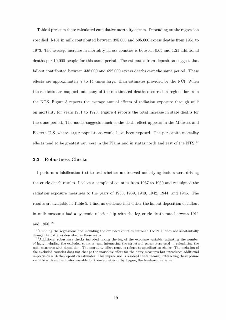
Table 4 presents these calculated cumulative mortality effects. Depending on the regression

specified, I-131 in milk contributed between 395,000 and 695,000 excess deaths from 1951 to

1973. The average increase in mortality across counties is between 0.65 and 1.21 additional

deaths per 10,000 people for this same period. The estimates from deposition suggest that

fallout contributed between 338,000 and 692,000 excess deaths over the same period. These

effects are approximately 7 to 14 times larger than estimates provided by the NCI. When

these effects are mapped out many of these estimated deaths occurred in regions far from

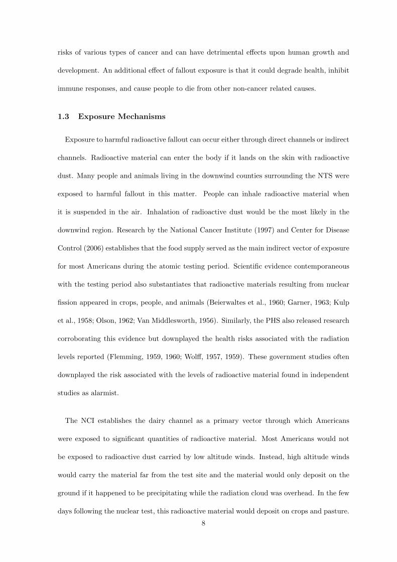
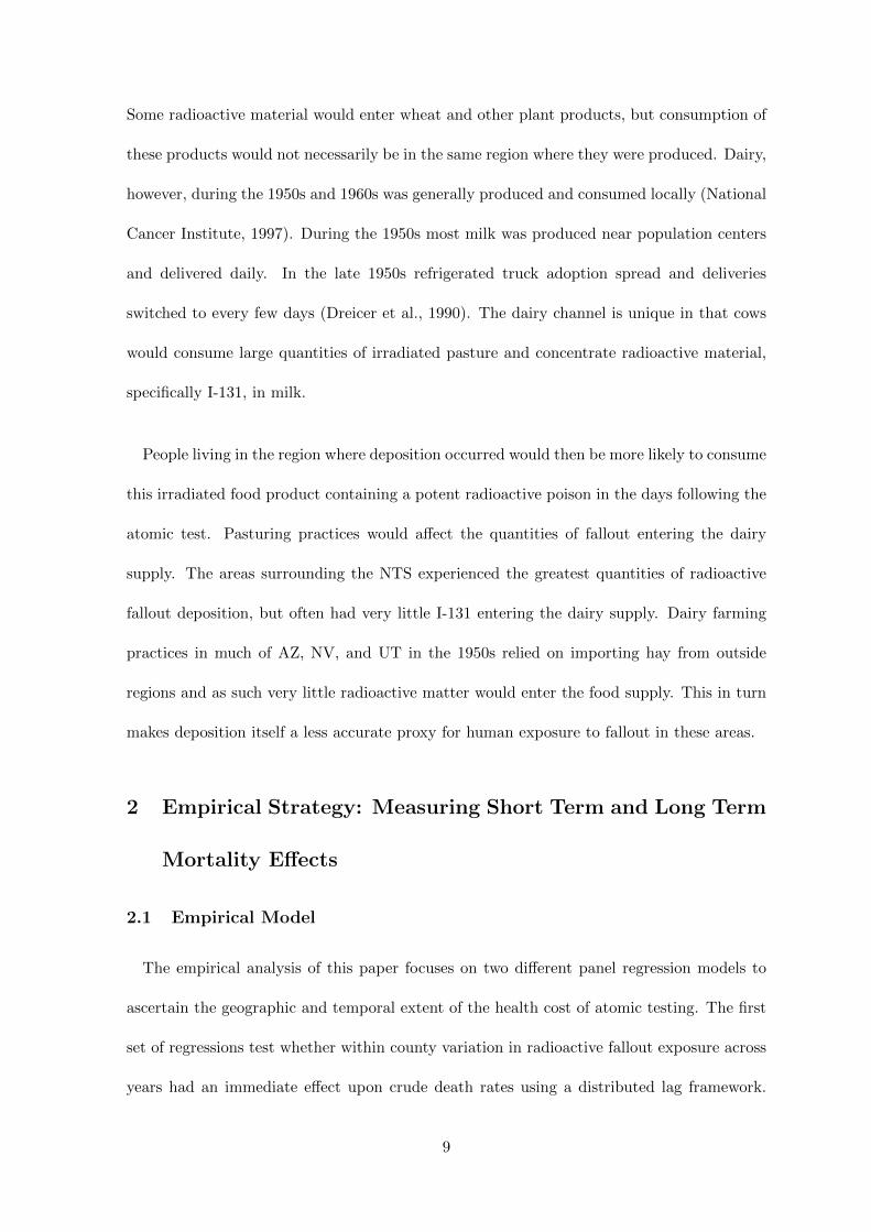
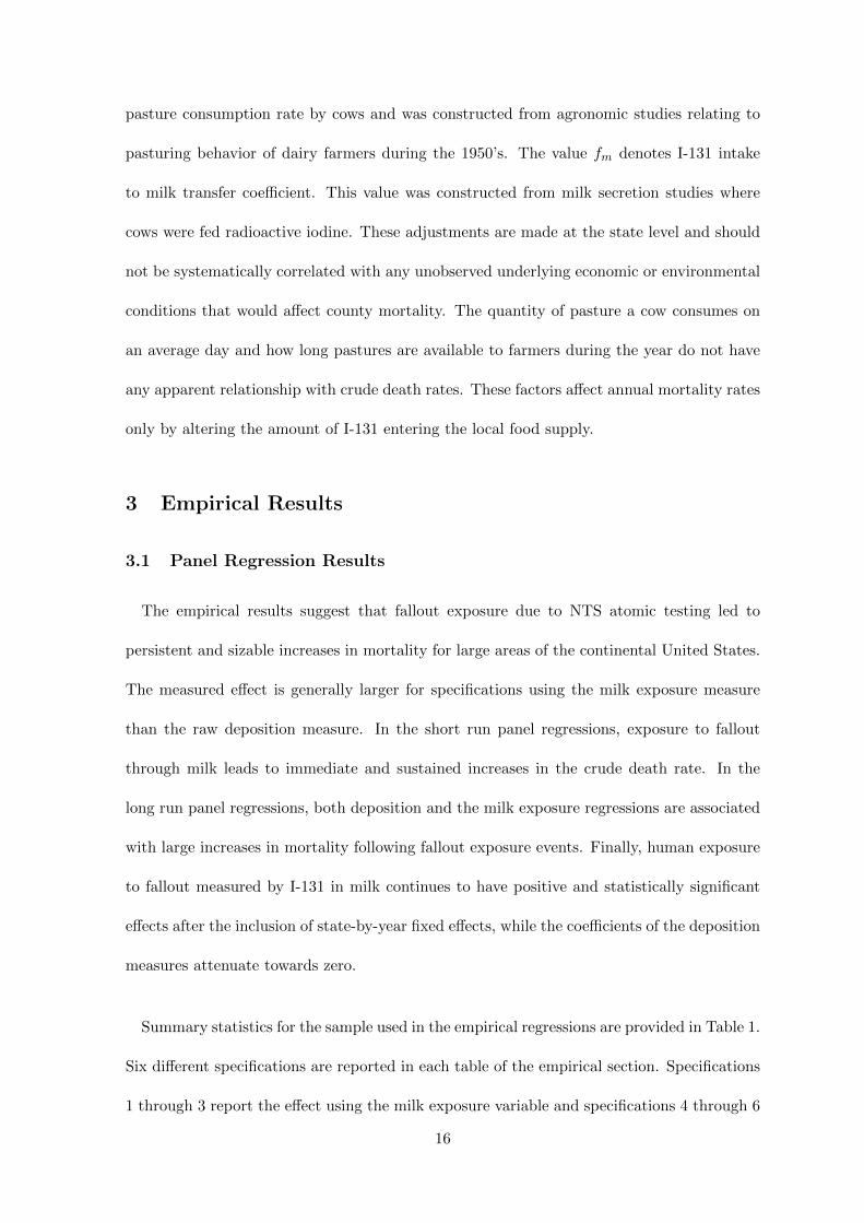
the NTS. Figure 3 reports the average annual effects of radiation exposure through milk

on mortality for years 1951 to 1973. Figure 4 reports the total increase in state deaths for

the same period. The model suggests much of the death effect appears in the Midwest and

Eastern U.S. where larger populations would have been exposed. The per capita mortality

effects tend to be greatest out west in the Plains and in states north and east of the NTS.17

3.3 Robustness Checks

I perform a falsification test to test whether unobserved underlying factors were driving

the crude death results. I select a sample of counties from 1937 to 1950 and reassigned the

radiation exposure measures to the years of 1938, 1939, 1940, 1942, 1944, and 1945. The

results are available in Table 5. I find no evidence that either the fallout deposition or fallout

in milk measures had a systemic relationship with the log crude death rate between 1911

and 1950.18

17Running the regressions and including the excluded counties surround the NTS does not substantiallychange the patterns described in these maps.

18Additional robustness checks included taking the log of the exposure variable, adjusting the numberof lags, including the excluded counties, and interacting the structural parameters used in calculating themilk measures with deposition. The mortality effect remains robust to specification choice. The inclusion ofthe excluded counties does not change the mortality effect for the dairy measures but introduces additionalimprecision with the deposition estimates. This imprecision is resolved either through interacting the exposurevariable with and indicator variable for these counties or by logging the treatment variable.

19

4 Policy Implications of Nuclear Testing

America’s nuclear weapons program was (and still is) a costly national defense policy.

From 1940 to 1996 the estimated cost of America’s nuclear weapons program was approx-

imately $8.93 Trillion in 2016$ (Schwartz, 2011). These monetary costs, however, do not

fully capture the full social cost of America’s nuclear weapons program. Since the 1990’s

the Federal Government has paid some compensation to victims of America’s domestic nu-

clear weapons program. This compensation has focused on workers involved in the nuclear

weapons program and those who lived downwind of the NTS during the 1950’s. The U.S.

Department of Justice pays out compensation to domestic victims of the nuclear weapons

program through the Radiation Exposure Compensation Act. As of 2015 the U.S. Depart-

ment of Justice has paid out over $2 billion in compensation to victims (US Department of

Justice, 2016).

Policy makers often assign accounting values to human lives when evaluating policy deci-

sions. Viscusi (1993) and Viscusi and Aldy (2003) survey these valuations placed on human

life. From 1988 to 2000, valuations of human life by U.S. Federal Government agencies ranged

between $1.4 million and $8.8 million in 2016$. These values and my estimates from the

preferred specification place the value of lost life between $473 billion and $6,116 billion in

2016$. Costa and Kahn (2004) use a hedonic wage regressions on industrial sector mortality

risks to back out plausible market values for human life for each decade from 1940 to 1980.

Using their values, I estimate the value of lost life from ground deposition between $1.24

and $2.56 trillion in 2016$. The estimates from milk exposure places the value of lost life

between $1.17 and $2.63 trillion. The social cost of excess deaths attributable to atmospheric

testing at the NTS ranges from approximately 5.3 percent to 68.4 percent of the total cost of

America’s nuclear weapons program. These values, however likely understate the magnitude

of the social costs of this polluting and environmentally destructive activities. Exposure

20

to radioactive fallout likely made millions of people less healthy, negatively affected human

capital, and increased the cost of providing health services to these populations. These costs

are not fully captured by measuring the effect of nuclear testing upon mortality rates.

The cessation of atmospheric nuclear testing drastically reduced the release of harmful

radioactive material into the air and likely saved many American lives. Two policies restricted

atmospheric testing at the NTS. The first was a testing moratorium from 1958 to 1961, which

moved almost all nuclear tests underground. The signing of the Partial Nuclear Test Ban

Treaty ultimately ended all atmospheric nuclear tests by the U.S. in 1963. The cumulative

kilo-tonnage of the atmospheric tests analyzed in this paper’s data is 992.4kt. During the

moratorium period the cumulative tonnage of underground testing at the NTS from 1958 to

1963 was 621.9kt. From 1963 to 1992, the total tonnage of nuclear explosions at the NTS

was 34,327.9kt, approximately thirty-four times larger than the NTS atmospheric tests (US

Department of Energy, 2000).19

Assuming that the domestic mortality effect of atmospheric testing is proportional to the

tonnage of the weapons tests, one might estimate approximately how many American lives

were saved by the moratorium period and the Partial Nuclear Test Ban Treaty. Multiplying

the smallest and largest cumulative mortality effects by the ratio of the moratorium tonnage

to atmospheric tonnage suggests that the moratorium possibly saved between 212,000 and

435,000 lives. Employing the same back of the envelope calculation, the Partial Nuclear

Test Ban Treaty might have saved between 11.7 and 24.0 million American lives. These

calculations have some caveats. First, it is likely that the transition to underground testing

increased the size of the weapons tested. This likely would overestimate the potential effect

of shifting underground testing above ground. Second, even without the moratorium and

19For the NTS, almost all tests were underground from 1958 to 1963. Some underground tests did notreport bomb yields but instead ranges of yields. In these cases bomb yield was taken as the average value.In cases where the bomb yield was greater than a certain value, the lowest value was assigned.

21

treaty, there was mounting scientific and medical evidence that NTS activity were harmful to

public health. It is likely that atmospheric testing at the NTS would have become politically

untenable as more of the negative health effects associated with atmospheric testing became

more pronounced. Finally, continuation of atmospheric testing likely would have increased

repeated public exposure to radioactive fallout. This increase in average frequency of expo-

sure might alter the point estimates identified in the panel regressions. Therefore, using the

realized estimates might underestimate the potential effect of continued atmospheric testing

upon mortality patterns.

The location of the NTS in Nye County, Nevada might have contributed towards the

level of human exposure to radioactive pollution. In 1950, military and political leaders

narrowed down list of potential atomic bombing ranges to a few locations (Schwartz, 2011).

Other locations given serious consideration include the Trinity Test Site located in White

Sands, New Mexico and Cape Hatteras, North Carolina. I use AP2 model from Muller

et al. (2011) to construct a counter-factual scenario of potential pollution exposure from

these alternative nuclear testing ranges. Nicholas Muller provided me a county to county

matrix which measures the effect of pollution emissions from one source county on PM2.5

concentrations in all other counties. If radioactive dust created by atmospheric atomic tests

follows similar dispersal patterns as other pollutants, then AP2 can provide a counter-factual

scenario and rank counties by how polluting they could have been.

For all counties other than the source county, I weight the PM2.5 coefficients by county

population in 1950. I then sum the cumulative effect of a single unit of emissions for each

of the 3,100 source counties. This procedure allows me to rank the relative downwind effect

of locating the NTS in an alternative county. Counties are ranked from least polluting to

most polluting.20 If policy makers sought to minimize human exposure to fallout, then

20I rank the relative dirtiness of the three mentioned locations and the top and bottom five alternativelocations provided by the model in the Appendix.

22

the location of the NTS is quite fortunate. According to AP2, the NTS ranks 39th out of

3,100 counties. The White Sands and Cape Hatteras locations rank as the 953th and 495th

least potentially polluting locations. Relatively speaking, White Sands would have been 3.45

times more polluting than the NTS and Cape Hatteras would have been 2.25 times more

polluting.21 These results show that atmospheric testing in the continental U.S. could have

plausibly been much worse for American populations and public health if policy makers had

chosen an alternative location.

5 Conclusion

This paper explores the temporal and geographic extent of the harm caused by atmospheric

nuclear tests conducted in Nevada between 1951 and 1958. Using a new national dataset

of radiation deposition and quantities of I-131 in the dairy supply, this paper finds that

radiation exposure increased crude deaths in areas hundreds to thousands of miles from the

test site. The geographic scope of the mortality consequences of NTS activities is broader

than what previous research has shown. The largest health effects appear in areas far beyond

the scope of previous scientific and medical studies. The scientific and medical literature has

studied the effects of atmospheric testing on populations residing in Downwind counties in

Arizona, Nevada, and Utah. Counter-intuitively, the areas where fallout had the largest

impact on the crude death rate was not in the region surrounding the test site, but rather

in areas with moderate levels of radioactive fallout deposition in the interior of the country.

Due to pasturing practices, large quantities of fallout wound up in local dairy supplies in

these regions but not in the Downwind region. It is quite plausible that extrapolating out

the health effects from small samples of persons who lived around the NTS substantially

underestimates the health costs associated with atmospheric testing.

21Intuitively the most polluting locations in the model would be the region surrounding New York City.These predictions are confirmed by the AP2 model. Interestingly, the Pacific Northwest, the Florida Keys,and Upstate Maine are locations that AP2 suggests would have been cleaner locations for testing than Nye,County.

23

The empirical results of this paper suggest that nuclear testing contributed to hundreds

of thousands of premature deaths in the United States between 1951 and 1972. The social

costs of these deaths range between $473 billion to over $6.1 trillion dollars in 2016$. These

losses dwarf the $2 billion in payments the Federal Government has made to domestic victims

of nuclear testing through the Radiation Exposure Compensation Act and are substantial

relative to the financial cost of the United States’ nuclear weapons program. It is likely that

the values of both the testing moratorium enacted in 1958 and the Partial Nuclear Test Ban

Treaty are understated. These political compromises likely saved hundreds of thousands of

additional lives at a minimum.

The evidence presented in this paper reveals that the health cost of domestic nuclear

testing is both larger and more expansive than previously thought. The mortality estimates

may understate the magnitude of the true number of deaths attributable to nuclear testing

and the magnitude of the health costs of this polluting defense policy. It is plausible that

these estimates are lower bounds of the true health effects. Migration and measurement

error in treatment introduces attenuation bias, and the health effects of radiation exposure

may only appear later in life for many individuals. Millions of people who grew up during

the testing period are now retiring from the labor force and are drawing upon Medicare and

other government provided services. Nuclear testing may have made an entire generation

of people less healthy and thus increased the cost of providing health care well into the

present. This paper reveals that there are more casualties of the Cold War than previously

thought, but the extent to which society still bears the costs of the Cold War remains an

open question.

24

References

Almond, D., Chen, Y., Greenstone, M., and Li, H. (2009a). Winter Heating or Clean Air?

Unintended Impacts of China’s Huai River Policy. American Economic Review, 99(2):184–

90.

Almond, D. and Currie, J. (2011). Killing me softly: The fetal origins hypothesis. The

Journal of Economic Perspectives, 25(3):153–172.

Almond, D., Edlund, L., and Palme, M. a. (2009b). Chernobyl’s subclinical legacy: prenatal

exposure to radioactive fallout and school outcomes in sweden. Quarterly Journal of

Economics, 124(4):1729–1772.

Bailey, M., Clay, K., Fishback, P., Haines, M., Kantor, S., Severnini, E., and Wentz, A.

(2016). U.S. County-Level Natality and Mortality Data. Dataset ICPSR36603-v1, Inter-

university Consortium for Political and Social Research, Ann Arbor, MI.

Ball, H. (1986). Justice downwind: America’s atomic testing program in the 1950s. Oxford

Press, New York, NY.

Barreca, A., Clay, K., and Tarr, J. (2014). Coal, Smoke, and Death: Bituminous Coal and

American Home Heating. Working Paper 19881, National Bureau of Economic Research.

DOI: 10.3386/w19881.

Beierwaltes, W. H., Crane, H. R., Wegst, A., Spafford, N. R., and Carr, E. A. (1960).

Radioactive iodine concentration in the fetal human thyroid gland from fall-out. JAMA,

173(17):1895–1902.

Black, S. E., Butikofer, A., Devereux, P. J., and Salvanes, K. G. (2013). This is only a test?

long-run impacts of prenatal exposure to radioactive fallout. Working Paper w18987,

National Bureau of Economic Research.

25

Center for Disease Control (2006). Report on the Health Consequences to the American Pop-

ulation from Nuclear Weapons Tests Conducted by the United States and Other Nations.

Technical report.

Clay, K., Lewis, J., and Severnini, E. (2016). Canary in a Coal Mine: Infant Mortality,

Property Values, and Tradeoffs Associated with Mid-20th Century Air Pollution. Working

Paper 22155, National Bureau of Economic Research.

Clay, K., Troesken, W., and Haines, M. (2014). Lead and mortality. Review of Economics

and Statistics, 96(3):458–470.

Costa, D. L. and Kahn, M. E. (2004). Changes in the Value of Life, 1940–1980. Journal of

risk and Uncertainty, 29(2):159–180.

Currie, J. (2013). Pollution and Infant Health. Child development perspectives, 7(4):237–242.

Currie, J., Davis, L., Greenstone, M., and Walker, R. (2015). Environmental health risks

and housing values: evidence from 1,600 toxic plant openings and closings. The American

economic review, 105(2):678–709.

Danzer, A. M. and Danzer, N. (2016). The long-run consequences of Chernobyl: Evidence on

subjective well-being, mental health and welfare. Journal of Public Economics, 135:47–60.

Dreicer, M., Bouville, A., and Wachholz, B. W. (1990). Pasture practices, milk distribution,

and consumption in the continental US in the 1950s. Health physics, 59(5):627–636.

Flemming, A. S. (1959). Public exposure to radiation. Public health reports, 74(5):441.

Flemming, A. S. (1960). Strontium 90 content of wheat. Public health reports, 75(7):674.

Fradkin, P. L. (2004). Fallout: An American Nuclear Tragedy. Big Earth Publishing.

Garner, R. J. (1963). Environmental contamination and grazing animals. Health physics,

9(6):597–605.

26

Gilbert, E. S., Huang, L., Bouville, A., Berg, C. D., and Ron, E. (2010). Thyroid cancer

rates and 131i doses from Nevada atmospheric nuclear bomb tests: an update. Radiation

research, 173(5):659–664.

Hanlon, W. W. (2015). Pollution and Mortality in the 19th Century. Working Paper 21647,

National Bureau of Economic Research.

Isen, A., Rossin-Slater, M., and Walker, W. R. (2017). Every breath you take—Every dollar

you’ll make: The long-term consequences of the Clean Air Act of 1970. Journal of Political

Economy, 125(3):848–902.

Kerber, R. A., Till, J. E., Simon, S. L., Lyon, J. L., Thomas, D. C., Preston-Martin, S.,

Rallison, M. L., Lloyd, R. D., and Stevens, W. (1993). A cohort study of thyroid disease

in relation to fallout from nuclear weapons testing. Jama, 270(17):2076–2082.

Kulp, J. L., Slakter, R., and others (1958). Current strontium-90 level in diet in United

states. American Association for the Advancement of Science. Science, 128:85–86.

LeBaron, W. D. (1998). America’s nuclear legacy. Nova Publishers.

Lee, S. (1999). Changes in the pattern of growth in stature related to prenatal exposure to

ionizing radiation. International journal of radiation biology, 75(11):1449–1458.

Lehmann, H. and Wadsworth, J. (2011). The impact of Chernobyl on health and labour

market performance. Journal of health economics, 30(5):843–857.

Muller, N. Z., Mendelsohn, R., and Nordhaus, W. (2011). Environmental Accounting for

Pollution in the United States Economy. American Economic Review, 101(5):1649–1675.

National Cancer Institute (1997). Estimated Exposures and Thyroid Doses Received by the

American People from Iodine-131 in Fallout Following Nevada Atmospheric Nuclear Bomb

Tests. Technical Report Technical Report.

27

Olson, T. A. (1962). Strontium-90 in the 1959 United States Wheat Crop. Science,

135(3508):1064–1064.

Otake, M. (1996). Threshold for radiation-related severe mental retardation in prenatally

exposed A-bomb survivors: a re-analysis. International journal of radiation biology,

70(6):755–763.

Otake, M., Fujikoshi, Y., Schull, W. J., and Izumi, S. (1993). A longitudinal study of growth

and development of stature among prenatally exposed atomic bomb survivors. Radiation

research, 134(1):94–101.

Schull, W. J. (1997). Brain damage among individuals exposed prenatally to ionizing radia-

tion: a 1993 review. Stem Cells, 15(S1):129–133.

Schwartz, S. I. (2011). Atomic audit: the costs and consequences of US nuclear weapons

since 1940. Brookings Institution Press.

Shibata, Y., Yamashita, S., Masyakin, V. B., Panasyuk, G. D., and Nagataki, S. (2001). 15

years after Chernobyl: new evidence of thyroid cancer. The Lancet, 358(9297):1965–1966.

Simon, S. L. and Bouville, A. (2015). Health effects of nuclear weapons testing. The Lancet,

386(9992):407–409.

Stevens, W., Thomas, D. C., Lyon, J. L., Till, J. E., Kerber, R. A., Simon, S. L., Lloyd,

R. D., Elghany, N. A., and Preston-Martin, S. (1990). Leukemia in Utah and radioactive

fallout from the Nevada test site: A case-control study. Jama, 264(5):585–591.

Troesken, W. (2008). Lead water pipes and infant mortality at the turn of the twentieth

century. Journal of Human Resources, 43(3):553–575.

US Department of Energy (2000). United States Nuclear Tests July 1945 through September

1992. Technical Report Report DOE/NV-209-REV 15, US DOE. Nevada Operations

Office, Las Vegas.

28

US Department of Justice (2016). RADIATION EXPOSURE COMPENSATION ACT.

Van Middlesworth, L. (1956). Radioactivity in thyroid glands following nuclear weapons

tests. Science, 123(3205):982–983.

Viscusi, W. K. (1993). The value of risks to life and health. Journal of economic literature,

31(4):1912–1946.

Viscusi, W. K. and Aldy, J. E. (2003). The value of a statistical life: a critical review of

market estimates throughout the world. Journal of risk and uncertainty, 27(1):5–76.

Williams, D. (2002). Cancer after nuclear fallout: lessons from the Chernobyl accident.

Nature Reviews Cancer, 2(7):543–549.

Wolff, A. H. (1957). Radioactivity in animal thyroid glands. Public health reports,

72(12):1121.

Wolff, A. H. (1959). Milk contamination in the Windscale incident. Public health reports,

74(1):42.

29

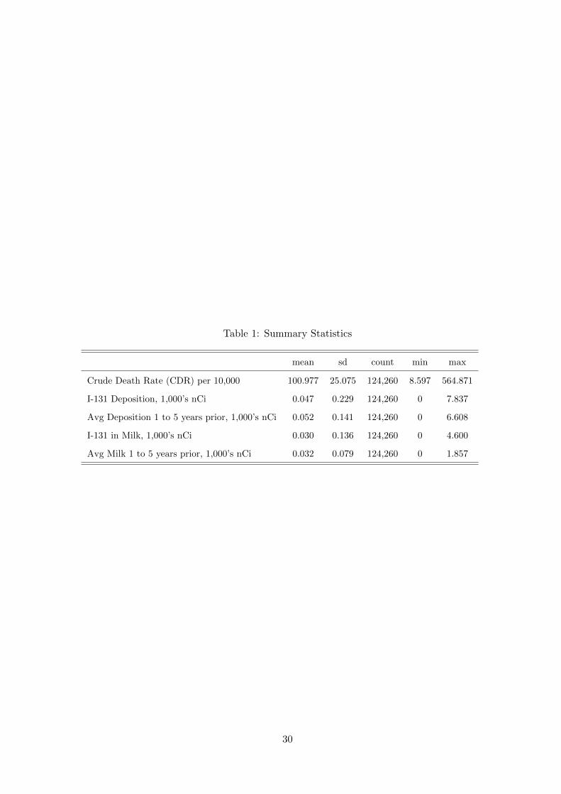
Table 1: Summary Statistics

mean sd count min max

Crude Death Rate (CDR) per 10,000 100.977 25.075 124,260 8.597 564.871

I-131 Deposition, 1,000’s nCi 0.047 0.229 124,260 0 7.837

Avg Deposition 1 to 5 years prior, 1,000’s nCi 0.052 0.141 124,260 0 6.608

I-131 in Milk, 1,000’s nCi 0.030 0.136 124,260 0 4.600

Avg Milk 1 to 5 years prior, 1,000’s nCi 0.032 0.079 124,260 0 1.857

30

Table 2: Short Run Mortality Effects, Crude Death Rate, 1940-1988

(1) (2) (3) (1) (2) (3)

Milk Exposure, 1,000’s nCi Deposition Exposure, 1,000’s nCi

Exposure, t -0.113 0.997∗∗ 2.469∗∗ 0.181 -0.352 0.635

(0.551) (0.505) (0.981) (0.333) (0.296) (0.457)

Exposure, t-1 1.475∗∗∗ 2.115∗∗∗ 4.286∗∗∗ 1.029∗∗∗ 0.415 0.949∗

(0.524) (0.461) (0.764) (0.297) (0.275) (0.566)

Exposure, t-2 2.006∗∗∗ 2.509∗∗∗ 4.379∗∗∗ 1.238∗∗∗ 0.689∗∗∗ 0.879∗∗

(0.570) (0.493) (0.937) (0.277) (0.246) (0.406)

Exposure, t-3 1.554∗∗∗ 1.378∗∗∗ 2.287∗∗∗ 0.884∗∗∗ 0.320 0.556

(0.514) (0.461) (0.852) (0.282) (0.279) (0.462)

Exposure, t-4 2.866∗∗∗ 2.664∗∗∗ 2.708∗∗∗ 1.370∗∗∗ 0.806∗∗∗ 0.531

(0.539) (0.497) (0.833) (0.321) (0.283) (0.366)

Year FE Yes Yes Yes Yes Yes Yes

County FE Yes Yes Yes Yes Yes Yes

State Time Trends No Yes No No Yes No

State Year FE No No Yes No No Yes

N 124,260 124,260 124,260 124,260 124,260 124,260

Adj r2 0.647 0.686 0.693 0.647 0.686 0.693

∗ p < 0.10, ∗∗ p < 0.05, ∗∗∗ p < 0.01All Standard Errors are Clustered by County. Exposure denotes the yearly cumulativeI-131 measures at the county level.

31

Table 3: Long Run Mortality Effects, Crude Death Rate, 1940-1988

(1) (2) (3) (4) (5) (6)


Exposure, t-1 to t-5 13.59∗∗∗ 11.29∗∗∗ 12.93∗∗∗ 7.734∗∗∗ 3.881∗∗∗ 1.878

(1.684) (1.584) (2.774) (1.264) (1.204) (2.083)

Exposure, t-6 to t-10 13.11∗∗∗ 8.676∗∗∗ 7.041∗∗ 6.797∗∗∗ 3.501∗∗∗ -0.362

(1.599) (1.565) (2.962) (1.263) (1.181) (1.794)

Exposure, t-11 to t-15 10.39∗∗∗ 4.854∗∗∗ 0.143 5.314∗∗∗ 2.346∗∗ -1.507

(1.662) (1.588) (2.888) (1.167) (1.018) (1.425)

Exposure, t-16 to t-20 7.239∗∗∗ 1.411 -7.894∗∗ 2.667∗∗ 0.0859 -5.502∗∗∗

(1.786) (1.680) (3.520) (1.140) (0.979) (1.353)

Exposure, t-21 to t-25 7.834∗∗∗ -2.317 -5.779∗∗ 2.513∗∗∗ 0.0434 -2.909∗∗∗

(1.915) (1.414) (2.801) (0.847) (0.587) (1.110)





N 124,260 124,260 124,260 124,260 124,260 124,260

Adj r2 0.648 0.686 0.693 0.648 0.686 0.693

∗ p < 0.10, ∗∗ p < 0.05, ∗∗∗ p < 0.01All Standard Errors are Clustered by County. Exposure denotes the pooled five yearaverages of cumulative I-131 measures at the county level.

32

Table 4: Changes in County Mortality Patterns Attributable to NTS Fallout, 1951 to 1973

I-131 In Local Milk

Mean SD Max Total Deaths

Specification 1 1.208 1.899 26.259 695,436.300

Specification 2 0.806 1.320 20.975 458,506.700

Specification 3 0.649 1.280 24.012 359,360.700

I-131 Ground Deposition

Mean SD Max Total Deaths

Specification 4 1.056 1.779 51.102 692,407.400

Specification 5 0.517 0.883 25.644 338,472.700

Specification 6 - - - -

Source: Author’s calculations

33

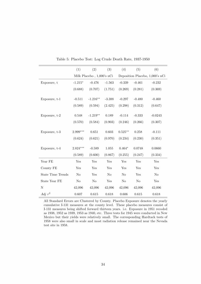
Table 5: Placebo Test: Log Crude Death Rate, 1937-1950

(1) (2) (3) (4) (5) (6)

Milk Placebo , 1,000’s nCi Deposition Placebo, 1,000’s nCi

Exposure, t -1.215∗ -0.476 -1.563 -0.339 -0.461 -0.232

(0.688) (0.707) (1.751) (0.269) (0.281) (0.369)

Exposure, t-1 -0.511 -1.216∗∗ -3.388 -0.297 -0.480 -0.460

(0.589) (0.594) (2.425) (0.298) (0.312) (0.647)

Exposure, t-2 0.548 -1.219∗∗ 0.189 -0.114 -0.333 -0.0243

(0.570) (0.584) (0.903) (0.246) (0.266) (0.307)

Exposure, t-3 2.999∗∗∗ 0.651 0.603 0.525∗∗ 0.258 -0.111

(0.624) (0.621) (0.970) (0.234) (0.230) (0.351)

Exposure, t-4 2.824∗∗∗ -0.589 1.055 0.464∗ 0.0748 0.0660

(0.589) (0.600) (0.867) (0.255) (0.247) (0.334)





N 42,096 42,096 42,096 42,096 42,096 42,096

Adj r2 0.607 0.615 0.618 0.606 0.615 0.618

All Standard Errors are Clustered by County. Placebo Exposure denotes the yearlycumulative I-131 measures at the county level. These placebo measures consist ofI-131 measures being shifted forward thirteen years. i.e. Exposure in 1951 recodedas 1938, 1952 as 1939, 1953 as 1940, etc. Three tests for 1945 were conducted in NewMexico but their yields were relatively small. The corresponding Hardtack tests of1958 were also small in scale and most radiation release remained near the Nevadatest site in 1958.

34

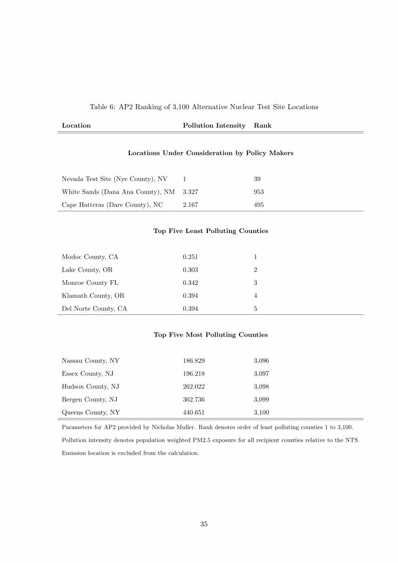
Table 6: AP2 Ranking of 3,100 Alternative Nuclear Test Site Locations

Location Pollution Intensity Rank

Locations Under Consideration by Policy Makers

Nevada Test Site (Nye County), NV 1 39

White Sands (Dana Ana County), NM 3.327 953

Cape Hatteras (Dare County), NC 2.167 495

Top Five Least Polluting Counties

Modoc County, CA 0.251 1

Lake County, OR 0.303 2

Monroe County FL 0.342 3

Klamath County, OR 0.394 4

Del Norte County, CA 0.394 5

Top Five Most Polluting Counties

Nassau County, NY 186.829 3,096

Essex County, NJ 196.218 3,097

Hudson County, NJ 262.022 3,098

Bergen County, NJ 362.736 3,099

Queens County, NY 440.651 3,100

Parameters for AP2 provided by Nicholas Muller. Rank denotes order of least polluting counties 1 to 3,100.

Pollution intensity denotes population weighted PM2.5 exposure for all recipient counties relative to the NTS.

Emission location is excluded from the calculation.

35

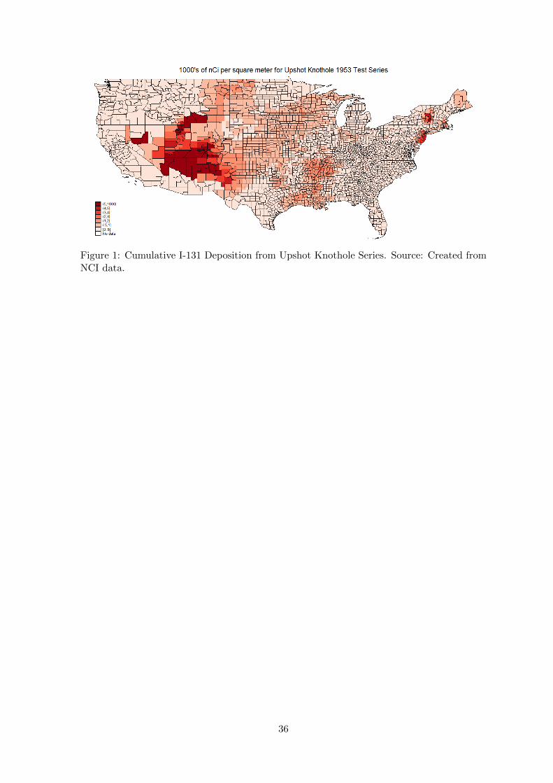
Figure 1: Cumulative I-131 Deposition from Upshot Knothole Series. Source: Created fromNCI data.

36

Figure 2: Cumulative I-131 Milk Measures from Upshot Knothole Series. Source: Createdfrom NCI data.

37

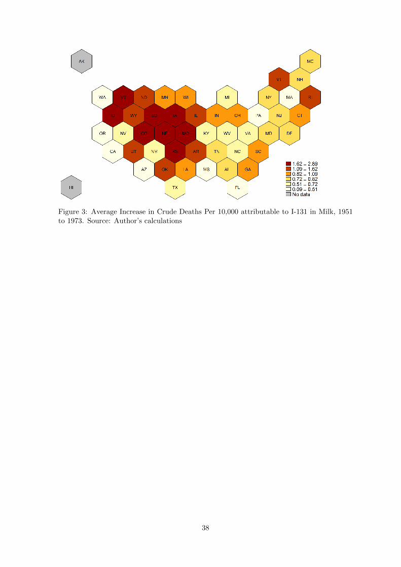
Figure 3: Average Increase in Crude Deaths Per 10,000 attributable to I-131 in Milk, 1951to 1973. Source: Author’s calculations

38

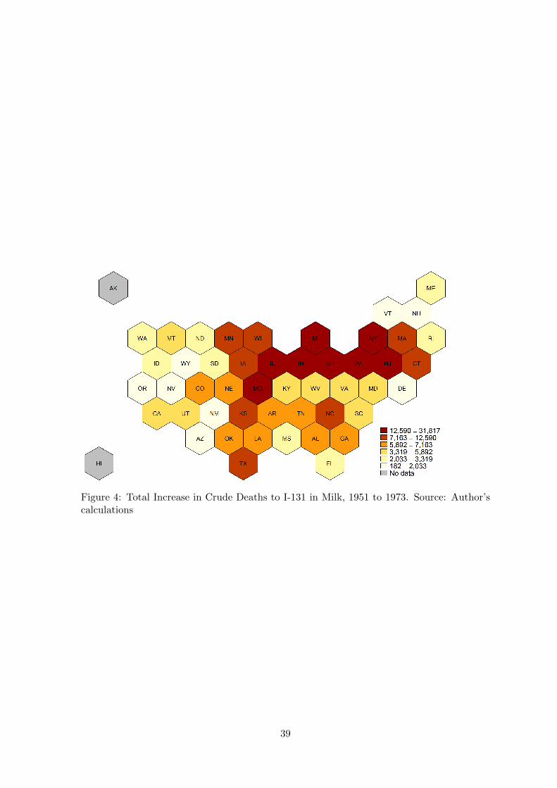
Figure 4: Total Increase in Crude Deaths to I-131 in Milk, 1951 to 1973. Source: Author’scalculations

39

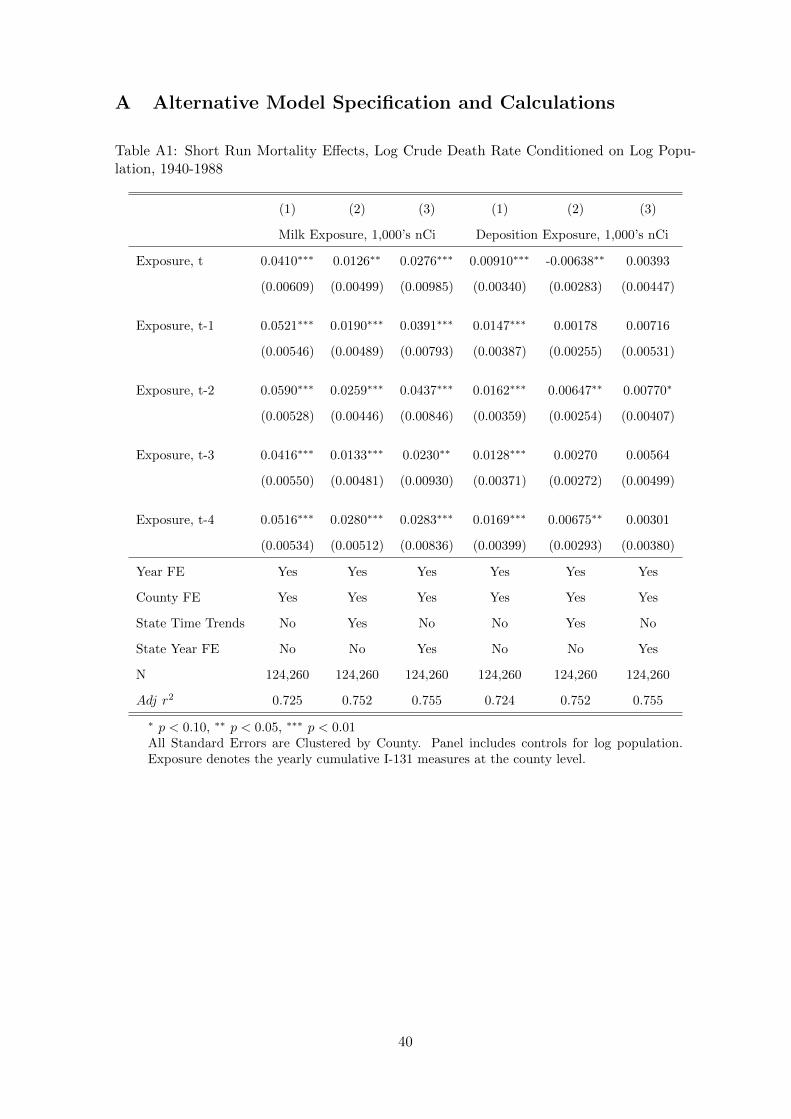
A Alternative Model Specification and Calculations

Table A1: Short Run Mortality Effects, Log Crude Death Rate Conditioned on Log Popu-lation, 1940-1988

(1) (2) (3) (1) (2) (3)


Exposure, t 0.0410∗∗∗ 0.0126∗∗ 0.0276∗∗∗ 0.00910∗∗∗ -0.00638∗∗ 0.00393

(0.00609) (0.00499) (0.00985) (0.00340) (0.00283) (0.00447)

Exposure, t-1 0.0521∗∗∗ 0.0190∗∗∗ 0.0391∗∗∗ 0.0147∗∗∗ 0.00178 0.00716

(0.00546) (0.00489) (0.00793) (0.00387) (0.00255) (0.00531)

Exposure, t-2 0.0590∗∗∗ 0.0259∗∗∗ 0.0437∗∗∗ 0.0162∗∗∗ 0.00647∗∗ 0.00770∗

(0.00528) (0.00446) (0.00846) (0.00359) (0.00254) (0.00407)

Exposure, t-3 0.0416∗∗∗ 0.0133∗∗∗ 0.0230∗∗ 0.0128∗∗∗ 0.00270 0.00564

(0.00550) (0.00481) (0.00930) (0.00371) (0.00272) (0.00499)

Exposure, t-4 0.0516∗∗∗ 0.0280∗∗∗ 0.0283∗∗∗ 0.0169∗∗∗ 0.00675∗∗ 0.00301

(0.00534) (0.00512) (0.00836) (0.00399) (0.00293) (0.00380)





N 124,260 124,260 124,260 124,260 124,260 124,260

Adj r2 0.725 0.752 0.755 0.724 0.752 0.755

∗ p < 0.10, ∗∗ p < 0.05, ∗∗∗ p < 0.01All Standard Errors are Clustered by County. Panel includes controls for log population.Exposure denotes the yearly cumulative I-131 measures at the county level.

40

Table A2: Short Run Mortality Effects, Log Crude Death Rate, 1940-1988

(1) (2) (3) (1) (2) (3)


Exposure, t 0.00776 0.0143∗∗ 0.0284∗∗ 0.00396 -0.00653∗∗ 0.00626

(0.00597) (0.00555) (0.0111) (0.00385) (0.00323) (0.00517)

Exposure, t-1 0.0216∗∗∗ 0.0236∗∗∗ 0.0441∗∗∗ 0.0127∗∗∗ 0.00283 0.00994∗

(0.00583) (0.00515) (0.00852) (0.00339) (0.00286) (0.00598)

Exposure, t-2 0.0293∗∗∗ 0.0302∗∗∗ 0.0510∗∗∗ 0.0159∗∗∗ 0.00771∗∗∗ 0.0107∗∗

(0.00584) (0.00498) (0.0103) (0.00319) (0.00268) (0.00480)

Exposure, t-3 0.0213∗∗∗ 0.0169∗∗∗ 0.0303∗∗∗ 0.0122∗∗∗ 0.00359 0.00792

(0.00562) (0.00501) (0.00961) (0.00343) (0.00299) (0.00559)

Exposure, t-4 0.0341∗∗∗ 0.0298∗∗∗ 0.0339∗∗∗ 0.0162∗∗∗ 0.00771∗∗ 0.00519

(0.00583) (0.00536) (0.00918) (0.00365) (0.00314) (0.00437)





N 124,260 124,260 124,260 124,260 124,260 124,260

Adj r2 0.661 0.699 0.705 0.661 0.698 0.705

∗ p < 0.10, ∗∗ p < 0.05, ∗∗∗ p < 0.01All Standard Errors are Clustered by County. Panel excludes controls for log population.Exposure denotes the yearly cumulative I-131 measures at the county level.

41

Table A3: Long Run Mortality Effects, Log Crude Death Rate Conditioned on Log Popula-tion, 1940-1988

(1) (2) (3) (1) (2) (3)


Exposure, t-1 to t-5 0.244∗∗∗ 0.113∗∗∗ 0.120∗∗∗ 0.0940∗∗∗ 0.0388∗∗∗ 0.0245

(0.0168) (0.0138) (0.0261) (0.0179) (0.0113) (0.0203)

Exposure, t-6 to t-10 0.147∗∗∗ 0.0783∗∗∗ 0.0477∗ 0.0760∗∗∗ 0.0385∗∗∗ 0.00872

(0.0137) (0.0127) (0.0261) (0.0146) (0.0108) (0.0169)

Exposure, t-11 to t-15 0.0958∗∗∗ 0.0507∗∗∗ -0.00304 0.0565∗∗∗ 0.0311∗∗∗ 0.0128

(0.0139) (0.0133) (0.0261) (0.0123) (0.00962) (0.0148)

Exposure, t-16 to t-20 0.0324∗∗ 0.0155 -0.0813∗∗∗ 0.0258∗∗ 0.0128 -0.0265∗∗

(0.0146) (0.0143) (0.0301) (0.0105) (0.00951) (0.0126)

Exposure, t-21 to t-25 -0.0411∗∗∗ -0.0113 -0.0674∗∗∗ 0.00583 0.00806 -0.0148

(0.0148) (0.0127) (0.0242) (0.00705) (0.00614) (0.0102)





N 124,260 124,260 124,260 124,260 124,260 124,260

Adj r2 0.726 0.752 0.755 0.725 0.752 0.755

∗ p < 0.10, ∗∗ p < 0.05, ∗∗∗ p < 0.01All Standard Errors are Clustered by County. Panel includes controls for log population. Ex-posure denotes the pooled five year averages of cumulative I-131 measures at the county level.

42

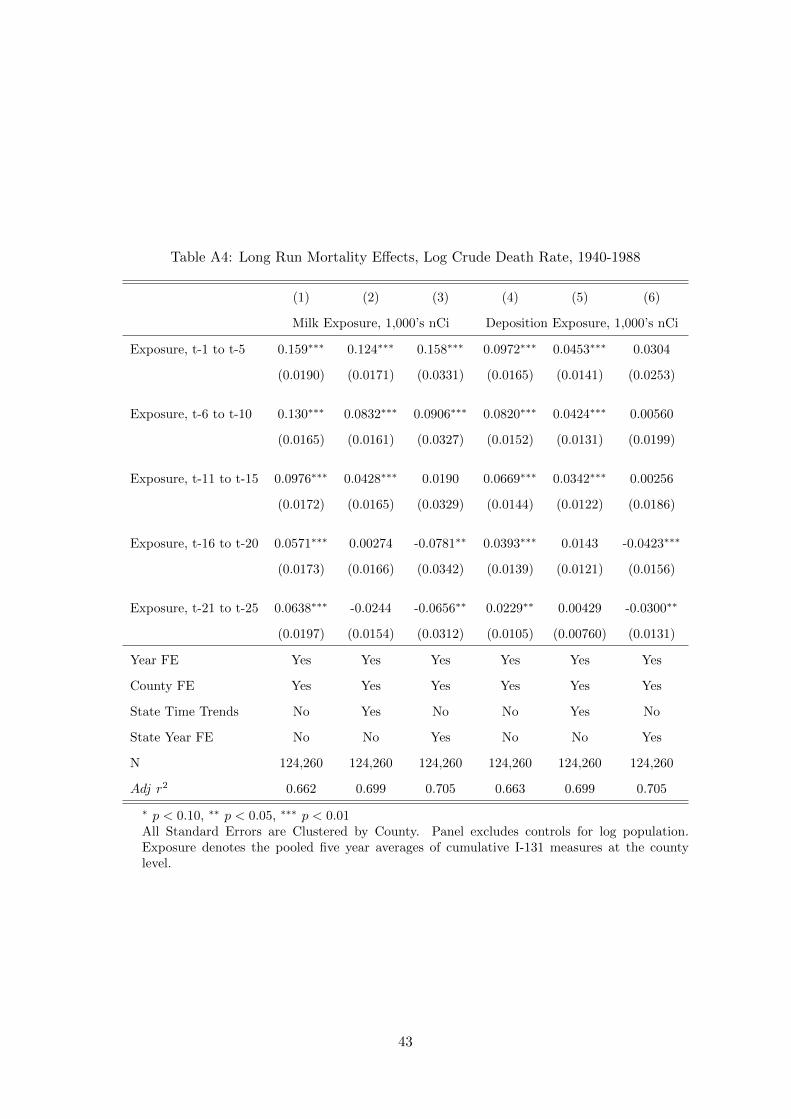
Table A4: Long Run Mortality Effects, Log Crude Death Rate, 1940-1988

(1) (2) (3) (4) (5) (6)


Exposure, t-1 to t-5 0.159∗∗∗ 0.124∗∗∗ 0.158∗∗∗ 0.0972∗∗∗ 0.0453∗∗∗ 0.0304

(0.0190) (0.0171) (0.0331) (0.0165) (0.0141) (0.0253)

Exposure, t-6 to t-10 0.130∗∗∗ 0.0832∗∗∗ 0.0906∗∗∗ 0.0820∗∗∗ 0.0424∗∗∗ 0.00560

(0.0165) (0.0161) (0.0327) (0.0152) (0.0131) (0.0199)

Exposure, t-11 to t-15 0.0976∗∗∗ 0.0428∗∗∗ 0.0190 0.0669∗∗∗ 0.0342∗∗∗ 0.00256

(0.0172) (0.0165) (0.0329) (0.0144) (0.0122) (0.0186)

Exposure, t-16 to t-20 0.0571∗∗∗ 0.00274 -0.0781∗∗ 0.0393∗∗∗ 0.0143 -0.0423∗∗∗

(0.0173) (0.0166) (0.0342) (0.0139) (0.0121) (0.0156)

Exposure, t-21 to t-25 0.0638∗∗∗ -0.0244 -0.0656∗∗ 0.0229∗∗ 0.00429 -0.0300∗∗

(0.0197) (0.0154) (0.0312) (0.0105) (0.00760) (0.0131)





N 124,260 124,260 124,260 124,260 124,260 124,260

Adj r2 0.662 0.699 0.705 0.663 0.699 0.705

∗ p < 0.10, ∗∗ p < 0.05, ∗∗∗ p < 0.01All Standard Errors are Clustered by County. Panel excludes controls for log population.Exposure denotes the pooled five year averages of cumulative I-131 measures at the countylevel.

43

Table A5: Changes in County Mortality Patterns Attributable to NTS Fallout, 1951 to 1973


Table A3 Mean SD Max Total Deaths

Specification 1 1.626 2.695 48.637 919,930.300

Specification 2 0.772 1.258 21.153 438,896.900

Specification 3 0.521 1.091 22.392 285,953.800



Specification 4 1.176 1.999 61.394 768,609.900

Specification 5 0.553 0.928 24.857 363,744.700

Specification 6 0.230 0.397 15.414 149,369.400

I-131 in Local Milk


Specification 1 1.265 2.009 30.404 724,033.300

Specification 2 0.797 1.337 23.163 450,844.700

Specification 3 0.865 1.603 30.219 482,489.200



Specification 4 1.283 2.158 63.592 840,690.700

Specification 5 0.623 1.046 28.852 409,208.300

Specification 6 0.191 0.425 19.209 119,680.600

Source: Author’s calculations.

44

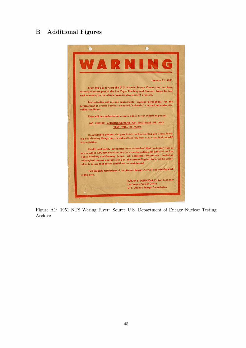
B Additional Figures

Figure A1: 1951 NTS Waring Flyer: Source U.S. Department of Energy Nuclear TestingArchive

45

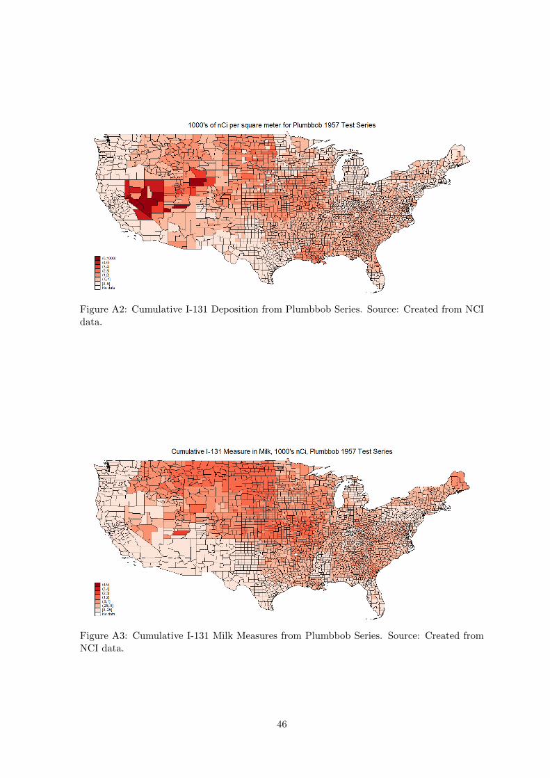
Figure A2: Cumulative I-131 Deposition from Plumbbob Series. Source: Created from NCIdata.

Figure A3: Cumulative I-131 Milk Measures from Plumbbob Series. Source: Created fromNCI data.

46

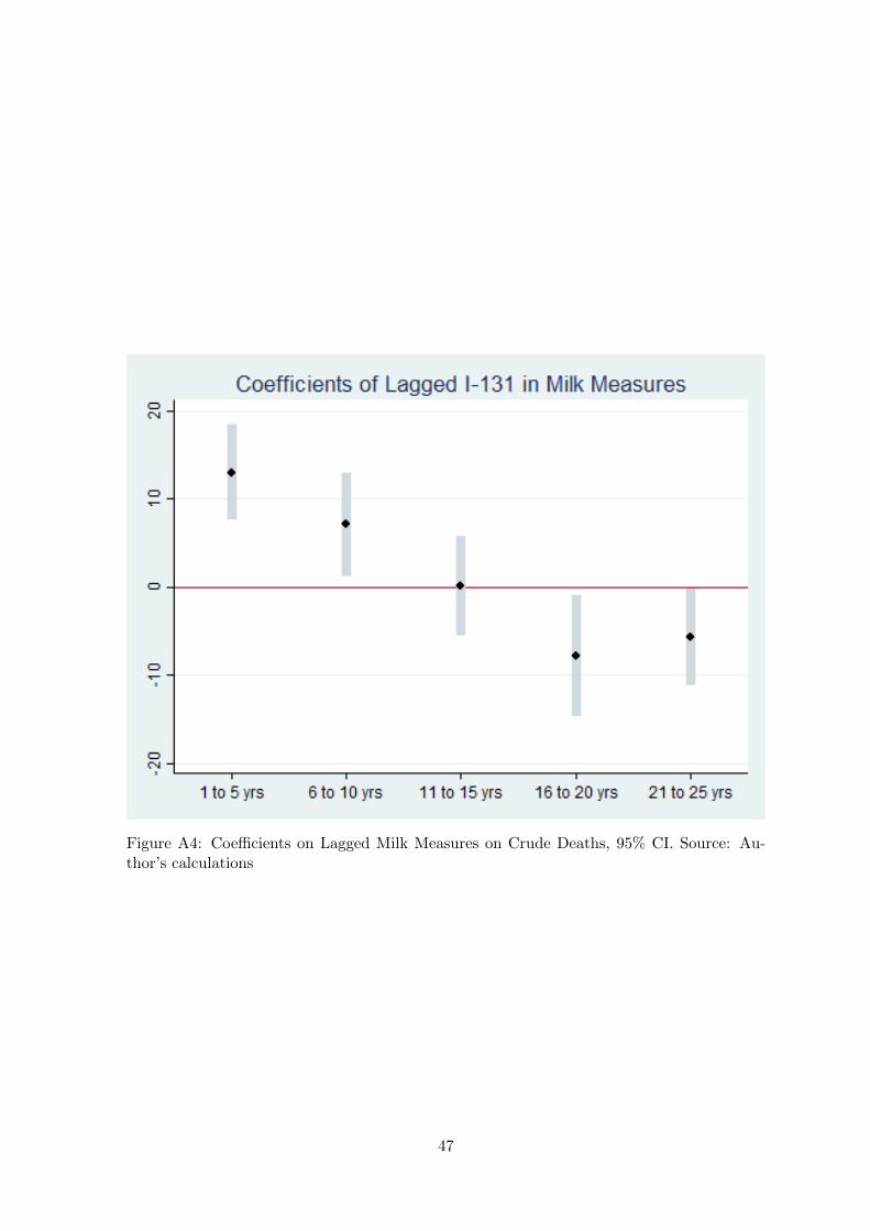
Figure A4: Coefficients on Lagged Milk Measures on Crude Deaths, 95% CI. Source: Au-thor’s calculations

47

Some Unintended Fallout from Defense Policy: … Unintended Fallout from Defense Policy: Measuring...

Documents

Transcript of Some Unintended Fallout from Defense Policy: … Unintended Fallout from Defense Policy: Measuring...