

Some topics in Bioinformatics: An introduction 1, Primary mathematical statistics 2, Sequence motif...
107
Some topics in Bioinformatics: An introduction 1, Primary mathematical statistics 2, Sequence motif discovery 2.1 Imbedded Markov chain 2.2 Search for patterns by alignment 3, HMM for protein secondary structure predicti on 4, Protein conformational letters and structure alignment 4.1 Conformational letters and substitution matrix 4.2 Fast pair structure alignment 4.3 Fast multiple structure alignment
-
date post
21-Dec-2015 -
Category
Documents
-
view
215 -
download
0
Transcript of Some topics in Bioinformatics: An introduction 1, Primary mathematical statistics 2, Sequence motif...
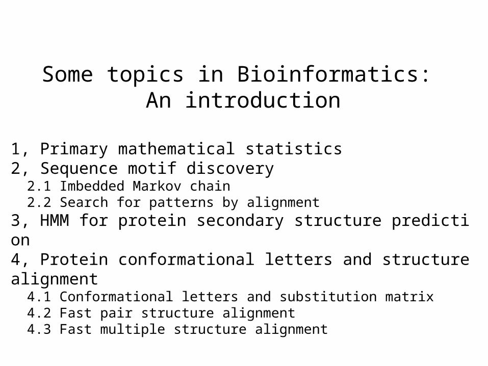
Some topics in Bioinformatics: An introduction
1, Primary mathematical statistics 2, Sequence motif discovery 2.1 Imbedded Markov chain 2.2 Search for patterns by alignment
3, HMM for protein secondary structure prediction 4, Protein conformational letters and structure alignment 4.1 Conformational letters and substitution matrix 4.2 Fast pair structure alignment 4.3 Fast multiple structure alignment

Some topics in Bioinformatics:
An Introduction
Primary Mathematical Statistics
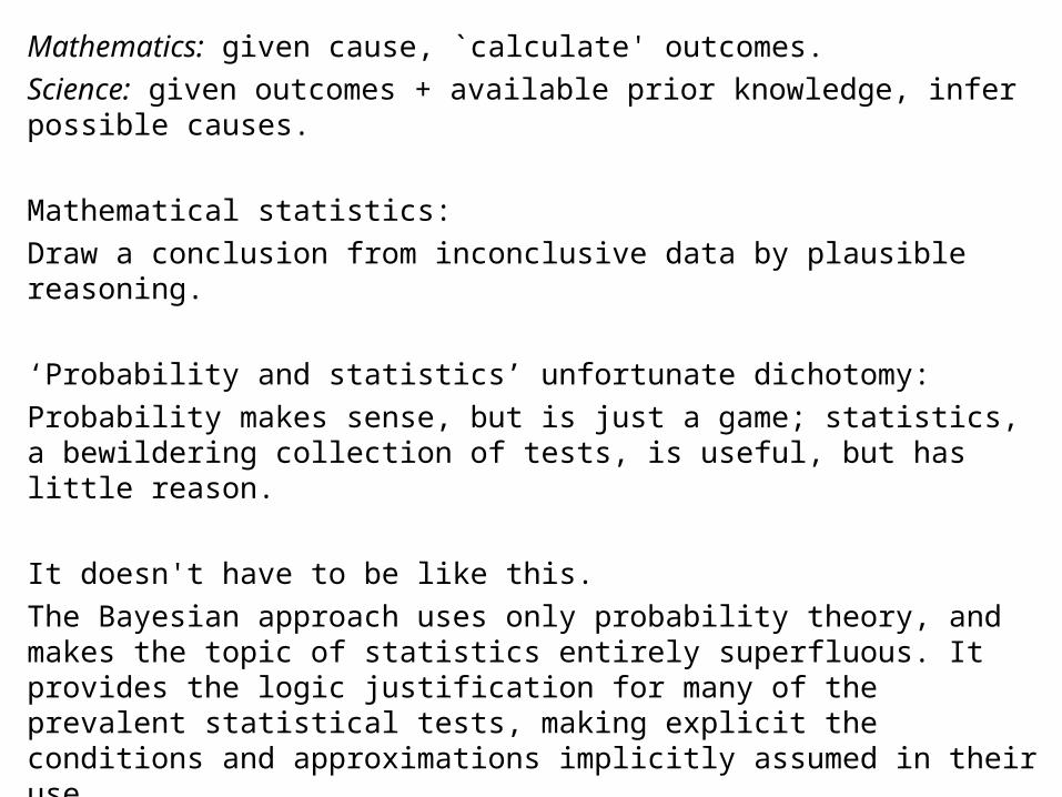
Mathematics: given cause, `calculate' outcomes.
Science: given outcomes + available prior knowledge, infer possible causes.
Mathematical statistics:
Draw a conclusion from inconclusive data by plausible reasoning.
‘Probability and statistics’ unfortunate dichotomy:
Probability makes sense, but is just a game; statistics, a bewildering collection of tests, is useful, but has little reason.
It doesn't have to be like this.
The Bayesian approach uses only probability theory, and makes the topic of statistics entirely superfluous. It provides the logic justification for many of the prevalent statistical tests, making explicit the conditions and approximations implicitly assumed in their use.
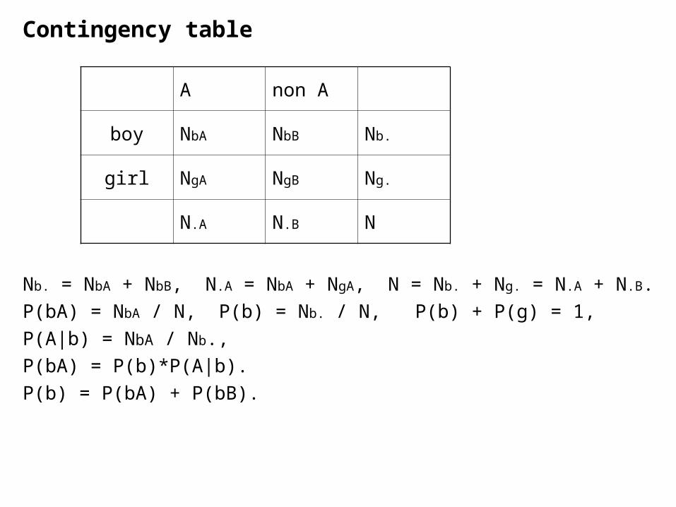
Contingency table
Nb. = NbA + NbB, N.A = NbA + NgA, N = Nb. + Ng. = N.A + N.B.
P(bA) = NbA / N, P(b) = Nb. / N, P(b) + P(g) = 1,
P(A|b) = NbA / Nb.,
P(bA) = P(b)*P(A|b).
P(b) = P(bA) + P(bB).
A non A
boy NbA NbB Nb.
girl NgA NgB Ng.
N.A N.B N

Three Formulae & Bayes’ TheoremSum rule:
Product rule:
I: the relevant background information at hand.Marginalization
is powerful device in dealing with nuisance parameters, which are necessary but of no intrinsic interest (e.g. background signal).
Bayes' theorem
posterior likelihood prior

By simple reinterpreting X as Model or Hypothesis and Y as Data, the formula becomes
which forms the foundation for data analysis. In some situations, such as model selection, the omitted denominator plays a crucial role, so is given the special name of evidence.
Parameter estimation:
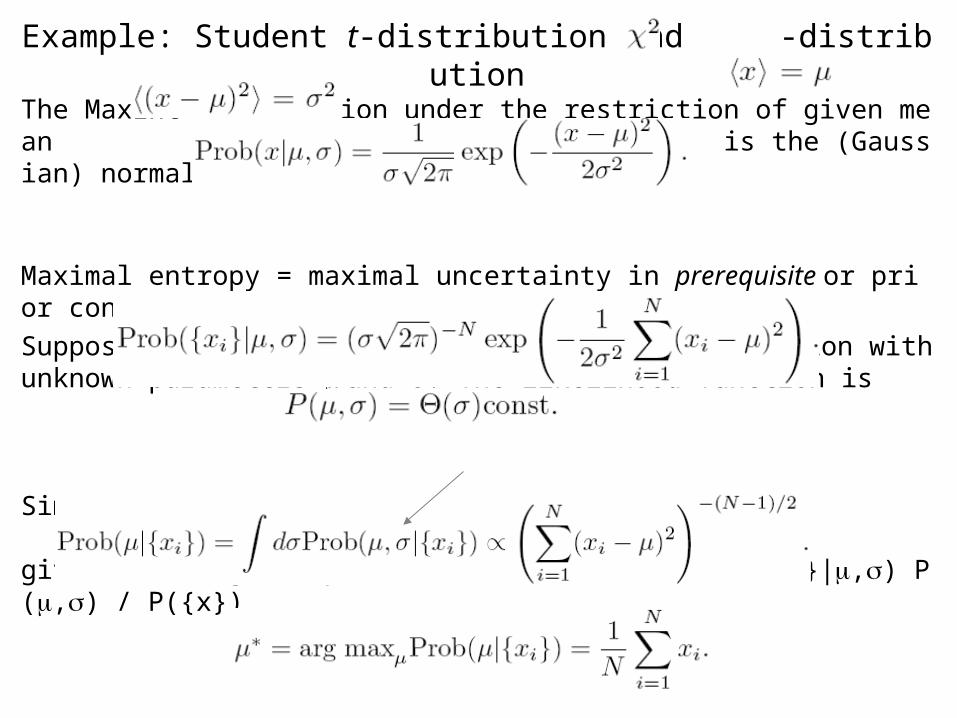
Example: Student t-distribution and -distributionThe MaxEnt distribution under the restriction of given mean and variance is the (Gaussian) normal distribution
Maximal entropy = maximal uncertainty in prerequisite or prior conditions.
Suppose { xi } are samples from a normal distribution with unknown parameters and . The likelihood function is
Simple flat prior
gives the marginal posterior P({x}|,) P(,) / P({x})
The estimate of parameter is

Introducing the decomposition
implies
which is a t-distribution. Another marginal posterior
is a -distribution.

Example: DNA sequence viewed as a outcome of die tossingA Nucleotide Die is a tetrahedron: {a, c, g, t}. The probability of observing a nucleotide a is p(a) = pa. Under the independent nonidentical distribution model, the probability to observe sequence s1s2…sn is
P(s1s2…sn | p) = p(s1)p(s2)…p(sn) =
Long repeats
Suppose the probability for nucleotide a is p. The length Y of a repeat of a has the geometric distribution
Thus, for the longest Ymax in n repeats, we have
For an N long sequence, it is estimated that n = (1-p)N. We have the
P-value = Prob(Ymax ≥ ymax)
≈
This discussion can be also used for word match between two sequences.

EntropiesShannon entropy:
Relative entropy distance of {p} from {q}
The equality is valid iff P and Q are identical. H measures the distance between P and Q. A related form (as leading terms of H) is
Conditional entropy
Mutual information (to measure independency or correlation)
Maximal entropy ⇔ Minimal likelihood a relative entropyMaximal uncertainty to `unknown' (premise); Minimal uncertainty to `known' (outcome).

Nonparametric estimate of distribution (Parzen kernel)Replace a single data point (-function) by a kernel function:
where d is the dimensionality, and kernel K satisfies some conditions. The Gaussian kernel is
For covariance the distance is one of Mahalanobis; for identity it is Euclidean. The optimal scale factor h may be fixed by minimize r or maximize m:
Pseudocounts viewed as a ‘kernel’.
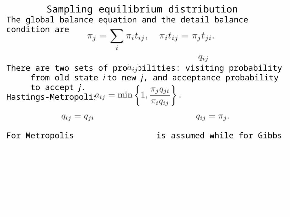
Sampling equilibrium distribution The global balance equation and the detail balance condition are
There are two sets of probabilities: visiting probability from old state i to new j, and acceptance probability to accept j. Hastings-Metropolis Algorithm uses
For Metropolis is assumed while for Gibbs

Jensen inequalityFor a random variable X and a continuous convex function g(x) on (a; b), we have
Proof: Suppose that and g’(x0) = k. From the convexity we have
which, by taking to be leads to
By taking expectation, this yields the inequality.
Discriminant analysis and cluster analysisSupervised learning and unsupervised learning

Example: Reduction of amino acid alphabetWe are interested in the mutual information I(C;a) between conformation and amino acids
Clustering amino acids leads to The difference between values of I after and before clustering is given by
which, by introducing
and defining is proportional to
with f(x) = x*log x. From the Jensen theorem, for the convex function x log x here we have , so I never increases after any step of clustering.

(Conditional) probabilities represent logical connections rather than causal ones. Example of Jaynes (1989): Given a bag of balls, five red and seven green. When a ball is selected at `random', the probability of drawing a red is 5/12. If the first ball is not returned to the bag, then it seems reasonable that the probability of obtaining a red or green ball on the second draw will depend on the outcome of the first. Now suppose that we are not told the outcome of the first draw, but are given the result of the second draw. Doesthe probability of the first draw being red or green change with the knowledge of the second? The answer ‘no' is incorrect. The error becomes obvious in the extreme case of one red and one green.
Probability as a degree-of-belief or plausibility; or a long-run relative frequency? Randomness is central to orthodox statistics and uncertainty inherent in Bayesian theory.
Necessity and contingency / certainty and randomness Deterministic and stochastic Deterministic and predictable

IntroductionIdentifying motifs or signals is a very common task. Patterns: Shed light on structure and function, used for classifying An example: the transcription regulatory sites (TFBSs).
Transcription factors and their binding sites (TFBS)
TATA boxTranscription start site (TSS)
RNA polymerase
gene regulatory
proteins

Such motifs are • generally short, • quite variable, and • often dispersed over a large distance.
Two ways for representing motifs:• the consensus sequence, or • a position-specific weight matrix (PSWM)• Profile HMM
Methods for Motif DiscoveryConsensus: Counting & evaluatingPSWM: Alignment & motif matrix updating

Imbedded Markov chain (IMC)Consensus: TATA-box: TATAAATA, Leucine zipper: L-X(6)-L-X(6)-L-X(6)-LCounting & evaluatingMotifs are identified as over- or under-represented oligomers.Count all possible DNA words of a certain length in an input set and then use statistics to evaluate over-represented words. Compare observed (in input set) with expected (in a background model)• possible k-tuples increases exponentially• limited to simple, short motifs with a highly conserved core.• complication due to overlaps of words.Independence approximation: ignore the correction of auto-correlation of pattern overlap, assume motifs occur independently at each position.DNA alphabet size is only 4. Simple patterns such as AAAA are easily found. Are they significant?Masking, high-order Markov (e.g. M3) modelsMany mathematical results, lack of easy implementary algorithms

Numerical enumerative techniquesImbedded Markov Chain (IMC) (Kleffe & Langbecker, 1990; Fu & Koutras, 1994)Example: x = 11011011, {0, 1} OverlapEnding States: prefixes arranged according to lengths. If a sequence belongs to state k, it must end with the string of state k, but not end with any strings with an index larger than k. State(110110) = 6, State(110111) = 2
11011011 11011011 11011011 11011011
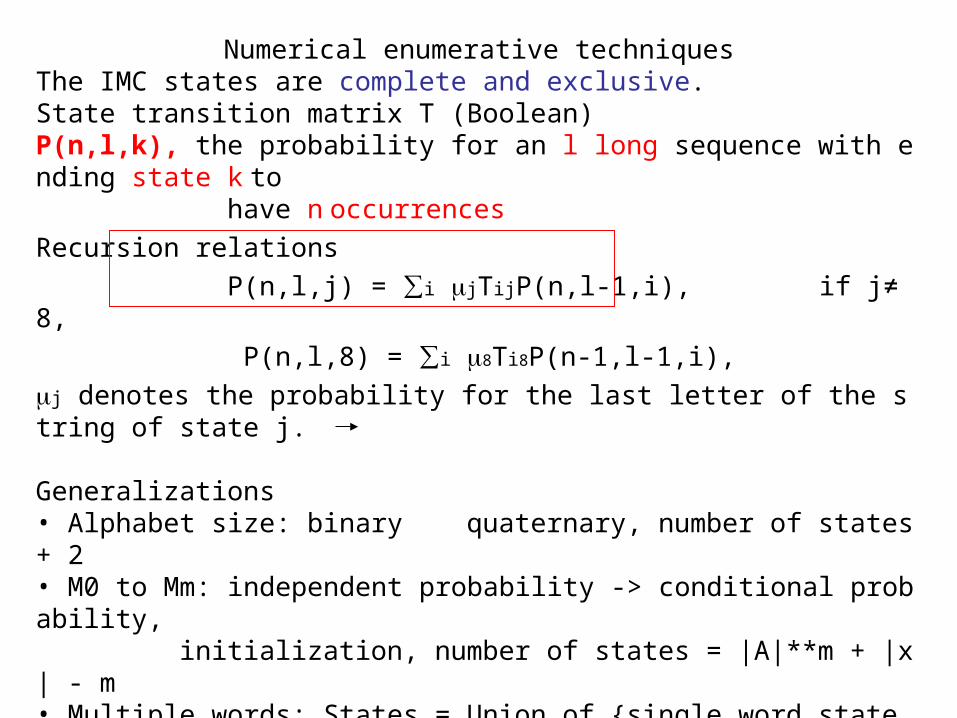
Numerical enumerative techniquesThe IMC states are complete and exclusive.State transition matrix T (Boolean)P(n,l,k), the probability for an l long sequence with ending state k to have n occurrencesRecursion relations P(n,l,j) = ∑i jTijP(n,l-1,i), if j≠ 8,
P(n,l,8) = ∑i 8Ti8P(n-1,l-1,i),
j denotes the probability for the last letter of the string of state j.
Generalizations• Alphabet size: binary quaternary, number of states + 2• M0 to Mm: independent probability -> conditional probability, initialization, number of states = |A|**m + |x| - m• Multiple words: States = Union of {single word states}DNA M3 model, x: TATAAAStates: TATAAA, TATAA, TATA, 64 triplets including TAT; 64+(6-3) = 67

Numerical enumerative techniquesKnown result for
Calculation of q, the probability with hits, and variation is not simple. Introduce (Q(1,L,k) determines q)
(R(1,L,k) determines <n>)
(S(1,L,k) determines )

Numerical enumerative techniquesRecursion relations
and similar relations for S. Using recursion relations for P, Q, R and S, we can calculate and to obtain q, and .

Search for pattern by alignmentBlock: Position Specific Weight Matrix (PSWM) Count number of occurrences of every letter at each position, A simple probabilistic models of sequence patterns; log likelihood or log odds; Alignment without gaps.Alignment score to determine optimal alignment for motif discoveryMatch score for locating known motif in a new sequence
AAATGACTCA AGATGAGTCA GAGAGAGTCA AGAAGAGTCA GAATGAGTCA AAATGACTCA AAGAGAGTCA GAATGAGTCA AAATGAGTCA consensus AAAWGAGTCA consensus with degenerate letter: W = A or T TGACTCWTTT motif on the complement strand

Motif search, a self-consistent problem
Motif positions weight matrixIf positions are known, the determination of matrix is straightforward.
If the matrix is known, we can scan sequences for positions with the matrix.
However, at the beginning we know neither the positions, nor the matrix.
Break the loop by iteration1. Make an initial guess of motif positions,2. Estimate weight matrix,3. Update motif positions,4. Convergent? End : Go to 2.
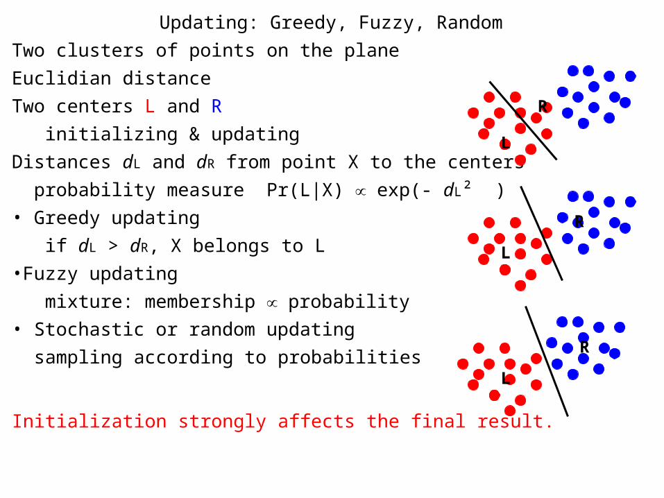
Updating: Greedy, Fuzzy, RandomTwo clusters of points on the planeEuclidian distanceTwo centers L and R initializing & updatingDistances dL and dR from point X to the centers probability measure Pr(L|X) ∝ exp(- dL² )
• Greedy updating if dL > dR, X belongs to L•Fuzzy updating mixture: membership ∝ probability• Stochastic or random updating sampling according to probabilities
Initialization strongly affects the final result.
R
L
R
L
R
L

Single motif in 30 sequencesVLHVLSDREKQIIDLTYIQNK 225 SQKETGDILGISQMHVSR LQRKAVKKLREALIEDPSMELMLDDREKEVIVGRFGLDLKKEK 198 TQREIAKELGISRSYVSR IEKRALMKMFHEFYRAEKEKRKMELRDLDLNLLVVFNQLLVDR 22 RVSITAENLGLTQPAVSN ALKRLRTSLQDPLFVRTHQGMETRYQTLELEKEFHFNRYLTRR 326 RRIEIAHALCLTERQIKI WFQNRRMKWKKENKTKGEPGSGHRILKEIEIPLLTAALAATRG 449 NQIRAADLLGLNRNTLRK KIRDLDIQVYRSGGMETKNLTIGERIRYRRKNLKH 22 TQRSLAKALKISHVSVSQ WERGDSEPTGKNLFALSKVLQC MNAY 5 TVSRLALDAGVSVHIVRD YLLRGLLRPVACTTGGYGLFDD ELVLAEVEQPLLDMVMQYTRG 73 NQTRAALMMGINRGTLRK KLKKYGMNSPQARAFLEQVFRRKQSLNSK 99 EKEEVAKKCGITPLQVRV WFINKRMRSKANKRNEALRIESALLNKIAML 25 GTEKTAEAVGVDKSQISR WKRDWIPKFSMLLAVLEWGVVDLLNLAKQPDAMTHPDGMQIKI 169 TRQEIGQIVGCSRETVGR ILKMLEDQNLISAHGKTIVVYGTR MEQRITLKDYAMRF 15 GQTKTAKDLGVYQSAINK AIHAGRKIFLTINADGSVYAEEVK MYKKDVIDHFG 12 TQRAVAKALGISDAAVSQ WKEVIPEKDAYRLEIVTAGALKYQMDNRVREACQYISDHLADSNF 196 DIASVAQHVCLSPSRLSH LFRQQLGISVLSWREDQRISQAKLYNLSRRFAQRGFSPREFRLTM 196 TRGDIGNYLGLTVETISR LLGRFQKSGMLAVKGKYITIENNDGLDERSQDIIRARWLDEDNKS 252 TLQELADRYGVSAERVRQ LEKNAMKKLRAAIEASEAQPEMERTLLTTALRHTQG 444 HKQEAARLLGWGRNTLTR KLKELGME MKAKKQETAA 11 TMKDVALKAKVSTATVSR ALMNPDKVSQATRNRVEKAAREVGETRREERIGQLLQELKRSDKL 23 HLKDAAALLGVSEMTIRR DLNNHSAPVVLLGGYIVLEPRSAS MA 3 TIKDVARLAGVSVATVSR VINNSPKASEASRLAVHSAMESLS MKPV 5 TLYDVAEYAGVSYQTVSR VVNQASHVSAKTREKVEAAMAELNDKSKVINSALELLNEVGIEGL 26 TTRKLAQKLGVEQPTLYW HVKNKRALLDALAIEMLDRHHTHFDEREALGTRVRIVEELLRGEM 67 SQRELKNELGAGIATITR GSNSLKAAPVELRQWLEEVLLKSDWLDNSLDERQRLIAALEKAGW 495 VQAKAARLLGMTPRQVAY RIQIMDITMPRLLNEREKQIMELRFGLVGEEEK 205 TQKDVADMMGISQSYISR LEKRIIKRLRKEFNKMVRRPKLTPEQWAQAGRLIAAGT 160 PRQKVAIIYDVGVSTLYK RFPAGDK MA 3 TIKDVAKRANVSTTTVSH VINKTRFVAEETRNAVWAAIKELH MA 3 TLKDIAIEAGVSLATVSR VLNDDPTLNVKEETKHRILEIAEKARQQEVFDLIRDHISQTGMPP 27 TRAEIAQRLGFRSPNAAE EHLKALARKGVIEIVSGASRGIRLTSTRKKANAITSSILNRIAIR 25 GQRKVADALGINESQISR WKGDFIPKMGMLLAVLEWGVEDEE

A R N D C Q E G ...A 4 -1 -2 -2 0 -1 -1 0 R -1 5 0 -2 -3 1 0 -2 N -2 0 6 1 -3 0 0 0 D -2 -2 1 6 -3 0 2 -1 C 0 -3 -3 -3 9 -3 -4 -3 Q -1 1 0 0 -3 5 2 -2 E -1 0 0 2 -4 2 5 -2 G 0 -2 0 -1 -3 -2 -2 6 ...
BLOck SUubstitution Matrix BLOSUM62 a matrix of amino acid similarity
SQKETGDILGISQMHVSRTQREIAKELGISRSYVSRRVSITAENLGLTQPAVSNRRIEIAHALCLTERQIKINQIRAADLLGLNRNTLRKTQRSLAKALKISHVSVSQTVSRLALDAGVSVHIVRDNQTRAALMMGINRGTLRKEKEEVAKKCGITPLQVRVGTEKTAEAVGVDKSQISRTRQEIGQIVGCSRETVGR. . .
weight matrix substitution matrix

Initialization by similarity
VLHVLSDREKQIIDLTYIQNKSQKETGDILGISQMHVSRLQRKAVKKLREALIEDPSMELM
LDDREKEVIVGRFGLDLKKEKTQREIAKELGISRSYVSRIEKRALMKMFHEFYRAEKEKRK
Start motif search with BLOSUM62. Two segments with a high similarity score are close neighbors. Motif is regarded as a group of close neighbors.
Take each window of width 18 as a seed, skip the sequence that the seed is in, search every sequence for the most similar neighbor of the seed in each sequence which has a similarity not less than s0, and find the score sum of these neighbors.
A seed and its near neighbors form a block or star tree, from which a primitive weight matrix and a substitution matrix can be deduced. The weight matrix or the substitution matrix (with the seed) is then used to scan each sequence for updating positions.

Top 10 seeds
Block of seed a2=198 (23 sequences) weight matrix
new block new weight matrix … (convergence)
28/30 correct; seed a25=205: 29/30 correct
Block of seed a2=198 New substitution matrix
new block (27 sequences) weight matrix … (convergence)
30/30 correct;Only greedy updating in use.
The motif might be wider. a2 = 198, 199, 197, 201,

MOTIF A MOTIF BKPVN 17 DFDLSAFAGAWHEIAK LPLE...NLVP 104 WVLATDYKNYAINYNC DYHPQTMK 25 GLDIQKVAGTWYSLAM AASD...ENKV 109 LVLDTDYKKYLLFCME NSAEKPVD 16 NFDWSNYHGKWWEVAK YPNS...ENVF 100 NVLSTDNKNYIIGYYC KYDERVKE 14 NFDKARFAGTWYAMAK KDPE...NDDH 105 WIIDTDYETFAVQYSC RLLNSTGR 27 NFNVEKINGEWHTIIL ASDK...FNTF 109 TIPKTDYDNFLMAHLI NEKD
Two motifs in 5 sequences

Top six seeds
Two motifs are seen, with the second shifted by 1.
If , two blocks have been correct.
New substitution matrix discovers the correct blocks.

Repeating motifs>>>SVLEIYDDEKNIEPALTKEFHKMYLDVAFEISLPPQMTALDASQPW 109 MLYWIANSLKVM DRDWLSDD 129 TKRKIVDKLFTI SPSG 145 GPFGGGPGQLSH LA 159 STYAAINALSLC DNIDGCWDRI 181 DRKGIYQWLISL KEPN 197 GGFKTCLEVGEV DTR 212 GIYCALSIATLL NILTEE 230 LTEGVLNYLKNC QNYE 246 GGFGSCPHVDEA HGG 261 YTFCATASLAIL RSMDQI 279 NVEKLLEWSSAR QLQEE 296 RGFCGRSNKLVD GC 310 YSFWVGGSAAIL EAFGYGQCF 331 NKHALRDYILYC CQEKEQ 349 PGLRDKPGAHSD FY 363 HTNYCLLGLAVA E 376 SSYSCTPNDSPH NIKCTPDRLIGSSKLTDVNPVYGLPIE 415 NVRKIIHYFKSN LSSPS
>>>L 74 QREKHFHYLKRG LRQLTDAYE CLDA 99 SRPWLCYWILHS LELLDEPIPQI 122 VATDVCQFLELC QSPD 138 GGFGGGPGQYPH LA 152 PTYAAVNALCII GTEEAYNVI 173 NREKLLQYLYSL KQPD 189 GSFLMHVGGEVD VR 203 SAYCAASVASLT NIITPD 221 LFEGTAEWIARC QNWE 237 GGIGGVPGMEAH GG 251 YTFCGLAALVIL KKERSL 269 NLKSLLQWVTSR QMRFE 286 GGFQGRCNKLVD GC 300 YSFWQAGLLPLL HRAL...HWMF 331 HQQALQEYILMC CQCPA 348 GGLLDKPGKSRD FY 362 HTCYCLSGLSIA QHFG...
>>>L 8 LKEKHIRYIESL DTKKHNFEYWLTEHLRLN 38 GIYWGLTALCVL DS PETF 56 VKEEVISFVLSC WDDKY 73 GAFAPFPRHDAH LL 87 TTLSAVQILATY DALDVLGKD 108 RKVRLISFIRGN QLED 124 GSFQGDRFGEVD TR 138 FVYTALSALSIL GELTSE 156 VVDPAVDFVLKC YNFD 172 GGFGLCPNAESH AA 186 QAFTCLGALAIA NKLDMLSDD 207 QLEEIGWWLCER QLPE 223 GGLNGRPSKLPD VC 237 YSWWVLSSLAII GRLDWI 255 NYEKLTEFILKC QDEKK 272 GGISDRPENEVD VF 286 HTVFGVAGLSLM GYDN...
>>>L 19 LLEKHADYIASY GSKKDDYEYCMSEYLRMS 49 GVYWGLTVMDLM GQ LHRM 67 NKEEILVFIKSC QHEC 83 GGVSASIGHDPH LL 97 YTLSAVQILTLY DSIHVI 115 NVDKVVAYVQSL QKED 131 GSFAGDIWGEID TR 145 FSFCAVATLALL GKLDAI 163 NVEKAIEFVLSC MNFD 179 GGFGCRPGSESH AG 193 QIYCCTGFLAIT SQLHQV 211 NSDLLGWWLCER QLPS 227 GGLNGRPEKLPD VC 241 YSWWVLASLKII GRLHWI 259 DREKLRSFILAC QDEET 276 GGFADRPGDMVD PF 290 HTLFGIAGLSLL GEEQ...
>>>V 12 VTKKHRKFFERH LQLLPSSHQGHDVNRMAIIFYSI...TINLPNTLFALLSMIMLRDYEYF ETIL 127 DKRSLARFVSKC QRPDRGSFVSCLDYKTNCGSSVDSDDLRFCYIAVAILYICGCRSKEDFDEYI 191 DTEKLLGYIMSQ QCYN 207 GAFGAHNEPHSG 219 YTSCALSTLALL SSLEKLSDK 240 FKEDTITWLLHR QV..DD 275 GGFQGRENKFAD TC 289 YAFWCLNSLHLL TKDWKMLC 309 QTELVTNYLLDR TQKTLT 327 GGFSKNDEEDAD LY 341 HSCLGSAALALI EGKF...
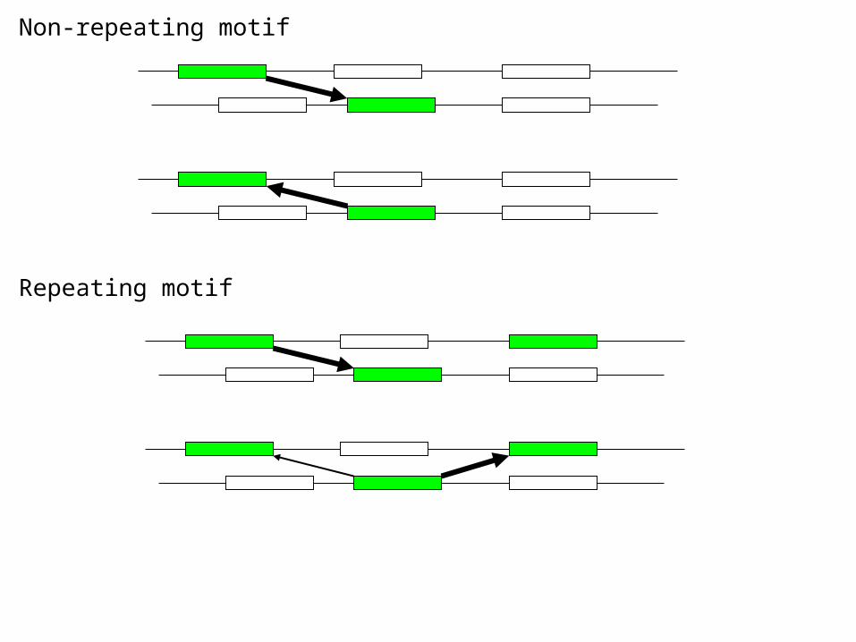
Non-repeating motif
Repeating motif
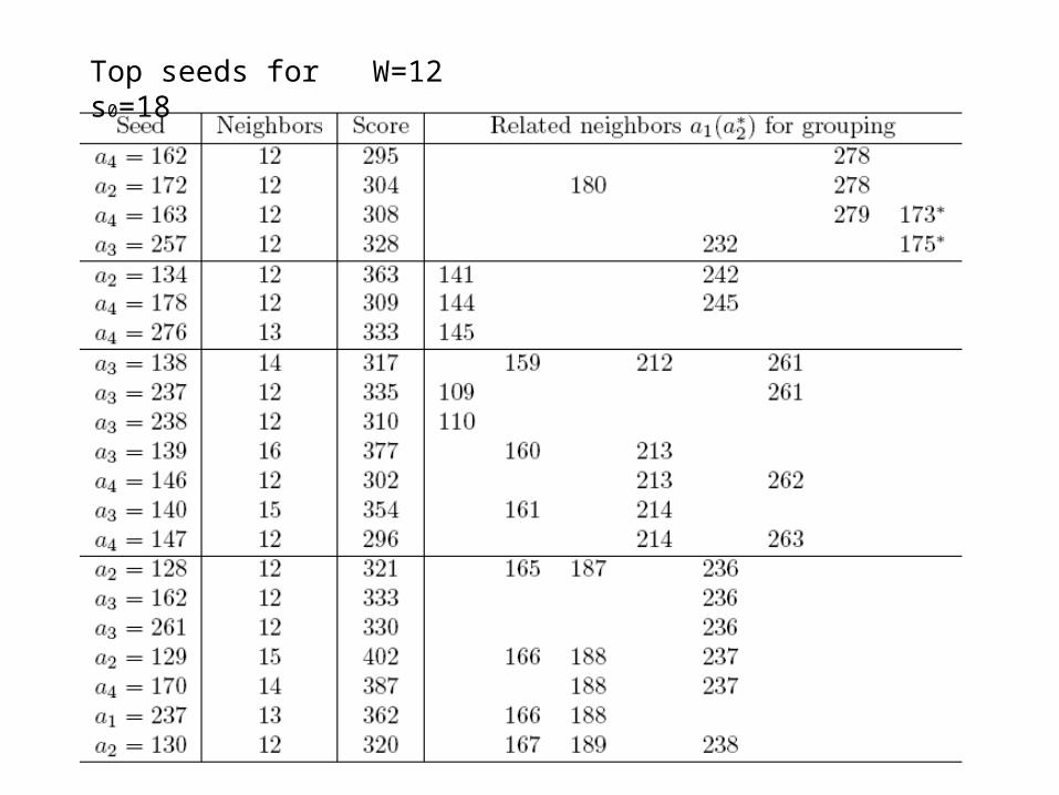
Top seeds for W=12 s0=18

Possible multiple motifs

From significant word to PSWM: Test on A. thaliana promoters Collect neighbors by similarity. Extend the boundaries of aligned block to widen the PSWM. A measure for distance between site to non-site
where q(i) for putative signal site, p0(i) for background non-site.
PSWMs from words TATAAAT and AACCCTA

Hidden Markov model (HMM)•Statistical summary representation for conserved region•Model stores probability of match, mismatch, insertions, anddeletions at each position in sequence•Alignment of conserved region not necessary, but helpful
delete
AAC insertACGA-TAAT123 match
Some topics in Bioinformatics:
An Introduction
Hidden Markov Model for
Protein Secondary Structure Prediction

Outline
• Protein structure• A brief review of secondary structure
prediction• Hidden Markov model: simple-
minded• Hidden Markov model: realistic• Discussion• References

c
N c
R
O
OH
HH
H cN c
R
O
OH
HH
H
c
N c
R
O
OH
HH
Hc
CO
R
N
H
L-formCORN-rule

Protein sequences are written in 20 letters (20 Naturally-occurring amino acid residues): AVCDE FGHIW KLMNY PQRST
Hydrophobic
Charged+-
Polar

Small
HydrophobicPolar
Aromatic
Aliphatic
Positive
Negative
TinyP
VI
F
Y
W
T
L
H
K
R
D
GA
C SN
E
QM

Cis-
Trans-
Residues form a directed chain
~5%Pro + 0.03%non-Pro < 0.3%

Rasmol ribbon diagram of GB1Helix, sheets and coil
Hydrogen-bond network
3D structure → secondary structure written in three letters: H, E, C.
H: E: C = 34.9: 21.8: 43.3
Amino acid sequence
a1a2 …
→
secondary structure
…EEEEEECCCCCEEEEECCCCCCCHHHHHHHHHHHHHCCCEEEEEEECCCCCEEEEE…

(In prediction stage)
Database Alignment
Single sequence based - - Nearest Neighbor + - Profile + +
Discriminant analysis Neural network (NN) approach Support vector machine (SVM)Probabilistic modelling

Bayes formula
Count of
Generally, P(x, y) = P(x|y)P(y),

Protein sequence A, {ai}, i=1,2,…,nSecondary structure sequence S, {si}, i=1,2,…,n
Secendary structure prediction: 1D amino acid sequences → 1D secondary structure sequenceAn old problem for more than 30 yearsDiscriminant analysis in the early stage
1. Simple Chou-fasman approach
Chou-Fasman’s propensity of amino acid to conformational state + independence approximation
One residue, one state

Parameter Training
Propensities q(a,s)
Counts (20x3) from a database: N(a, s)
sum over a → N(s),
sum over s → N(a),
sum over a and s → N
q(a,s) = [N(a,s) N] / [N(a) N(s)].

Propensity of amono acids to secondary structures
helix EAL HMQWVF KI DTSRC NY PG strand MVI CYFQLTW A RGD KSHNP E
Garnier-Osguthorpe-Robson Window version of propensity to the state at the center
-8-7-6-5-4-3-2-1 0+1+2+3+4+5+6+7+8 W R Q I C T V N A F L C E H S Y K
HEC
Based on assumption that each amino acid individually influences the propensity of the central residue to adopt a particular secondary structure. Each flanking position evaluated independently like a PSSM.
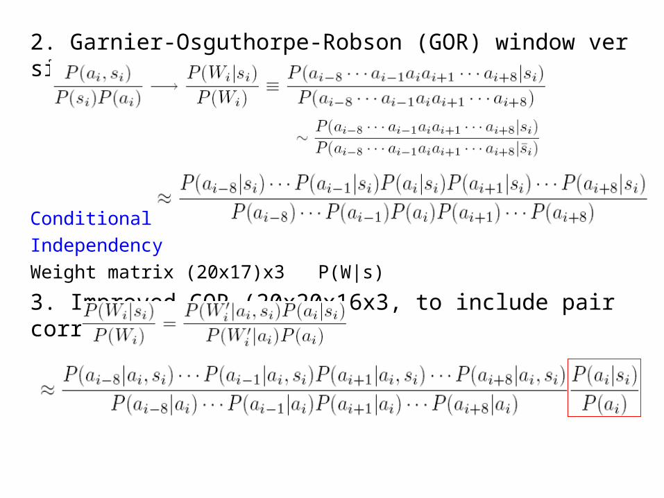
2. Garnier-Osguthorpe-Robson (GOR) window version
ConditionalIndependencyWeight matrix (20x17)x3 P(W|s)
3. Improved GOR (20x20x16x3, to include pair correlation)
Width determined by mutual information.
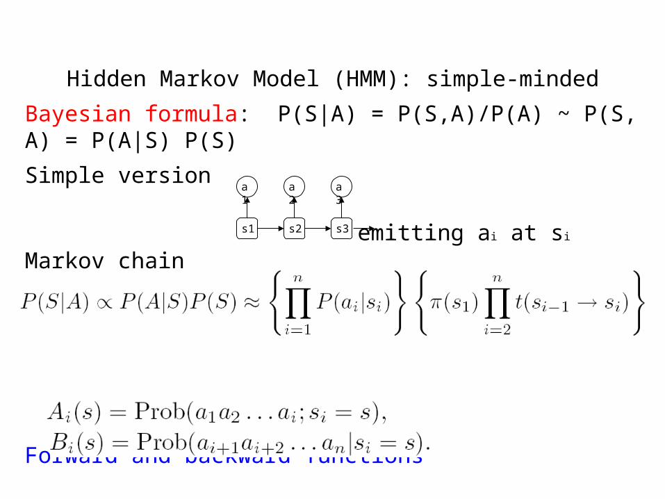
Hidden Markov Model (HMM): simple-mindedBayesian formula: P(S|A) = P(S,A)/P(A) ~ P(S,A) = P(A|S) P(S)
Simple version
emitting ai at si
Markov chain according to P(a|s)For hidden sequence
Forward and backward functions Head Tail
s1 s2 s3
a1 a2 a3

Initial conditions and recursion relations
Partition function

Prob(si=s, si+1=s’) = Ai(s) tss’ P(ai+1|s’) Bi+1(s’)/Z
This marginalization can be done for any segment, e.g. Prob(si:j)
Number of different S increases exponentially with |S|. Linear algorithm: Dynamic programming. Two interpretations of ‘operator’ as ‘sum’: Baum-Welch as ‘max’: Viterbi
Hidden Markov Model: Realistic
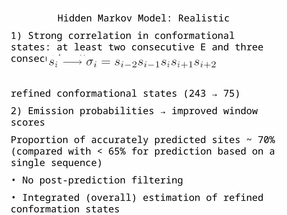
1) Strong correlation in conformational states: at least two consecutive E and three consecutive H
refined conformational states (243 → 75)
2) Emission probabilities → improved window scores
Proportion of accurately predicted sites ~ 70% (compared with < 65% for prediction based on a single sequence)
• No post-prediction filtering
• Integrated (overall) estimation of refined conformation states
• Measure of prediction confidence

Discussions
• HMM using refined conformational states and window scores is efficient for protein secondary structure prediction.
• Better score system should cover more correlation between conformation and sequence.
• Combining homologous information will improve the prediction accuracy.
• From secondary structure to 3D structure (structure codes: discretized 3D conformational states)

Three main ingredients of a HMM are • hidden states • Markov graph• scores
Model training is to determine the hidden parameters from the `observable' data. The extracted model parameters can then be used to perform further analysis, for example for pattern recognition. An HMM can be considered as the simplest dynamic Bayesian network.

The length distribution of helices
t (hhhhh → hhhhh) from string counting is 0.88; from length statistics: t (hhhhh → hhhhh) =
is 0.82. A simple approximation is to adjust the value at 0.83.
A more sophisticated way is to introduce more states for helices of different lengths, and make the geometric approximation only after certain length.
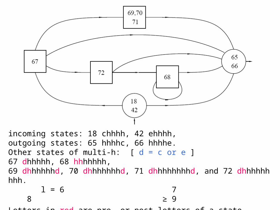
incoming states: 18 chhhh, 42 ehhhh, outgoing states: 65 hhhhc, 66 hhhhe. Other states of multi-h: [ d = c or e ]67 dhhhhh, 68 hhhhhhh,69 dhhhhhhd, 70 dhhhhhhhd, 71 dhhhhhhhhd, and 72 dhhhhhhhhh. l = 6 7 8 ≥ 9
Letters in red are pre- or post-letters of a state.
Scoring based on reduction of amino acid alphabets
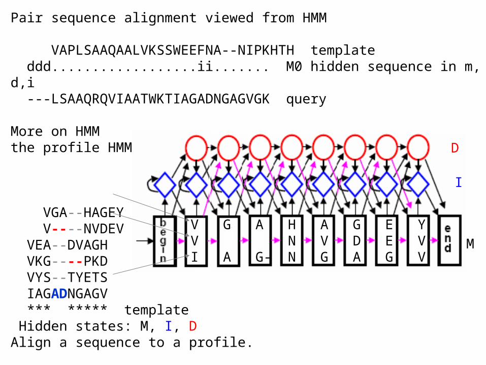
Pair sequence alignment viewed from HMM
VAPLSAAQAALVKSSWEEFNA--NIPKHTH template ddd..................ii....... M0 hidden sequence in m,d,i ---LSAAQRQVIAATWKTIAGADNGAGVGK query
More on HMMthe profile HMM
VGA--HAGEY V----NVDEV VEA--DVAGH VKG----PKD VYS--TYETS IAGADNGAGV *** ***** template Hidden states: M, I, D Align a sequence to a profile.
V G A H A G E YV N V D E VI A G- N G A G V
D
I
M

Hidden Markov modelA run in model M follows a Markovian path of states and generates a string S over a finite alphabet with probability PM(S). Typical HMM problems • Annotation: Given a model M and an observed string S, what is the most probable path through M that generates/outputs S. Viterbi• Classification: Given a model M and an observed string S, what is the total probability PM(S) of M generating S. Forward algorithm• Training: Given a set of training strings and a model structure, find transition and emission probabilities that make the training set most probable. [Silent state: emits no symbols.]Other HMM problemsComparison: Given two models, what is a measure of their likeliness. Consensus: Given a model M, find the string S that have the highest probability under the model.

Some topics in Bioinformatics:
An Introduction
Protein Conformational Letters
and Structure Alignment

• Protein structure alphabet: discretization of 3D continuous structure states
• Bridge 2’ structure and 3D structure
• Enhance correlation between sequence and structure
• Fast structure comparison
• Structure prediction (transplant 2’ structure prediction methods for 3D)
Conformational letters and substitution matrix
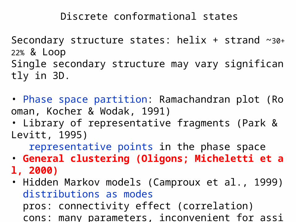
Discrete conformational states
Secondary structure states: helix + strand ~30+22% & LoopSingle secondary structure may vary significantly in 3D.
• Phase space partition: Ramachandran plot (Rooman, Kocher & Wodak, 1991)• Library of representative fragments (Park & Levitt, 1995) representative points in the phase space• General clustering (Oligons; Micheletti et al, 2000) • Hidden Markov models (Camproux et al., 1999) distributions as modes pros: connectivity effect (correlation) cons: many parameters, inconvenient for assigning states to short segments• Mixture model: clustering based on peaks in probability distribution

0
0
E B
N T
HI
F
PM
L
U
G
E
O
*
S
E: extendedB: betaI,H: alphaL,M: leftT,U: turnP: Pro-richG: Gly-richN: NH-NH conflictO: CO-CO conflictS: side chain conflict*: NH-CO conflict

AN APPROACH TO DETECTION OF PROTEIN STRUCTURAL MOTIFS USING AN ENCODING SCHEME OF BACKBONE CONFORMATIONSH. Matsuda, F. Taniguchi, A. Hashimoto
The placement of a protein backbone chain with an icosahedron in the Cartesian coordinates.

Representation of 3D backbone: C-alpha pseudobond angles
Four-residue fundamental unit: btb r1r2r3r4
1
23
4
b2t3b3b2
b3
t3
~ 3.8 A

S1
S2
Sliding windows

Pseudobonds: bend and torsion angles
dihedral angle, sign ~
n residures : btbtb...tb
n-2 bend angles + n-3 torsion angles = 2n-5 angles
For dominant trans, |r| = 3.8
[0 , ]
Origin is at r0, r01 falls on the x-axis, and r12 on the xy-plane. 1≡0
coordinates angles

Bend and torsion angles of pseudobonds
3.14 0.9 torsio
n -
3.14
3.14 1.9 bend 0.4 0.0
Peaks 1.55 1.10

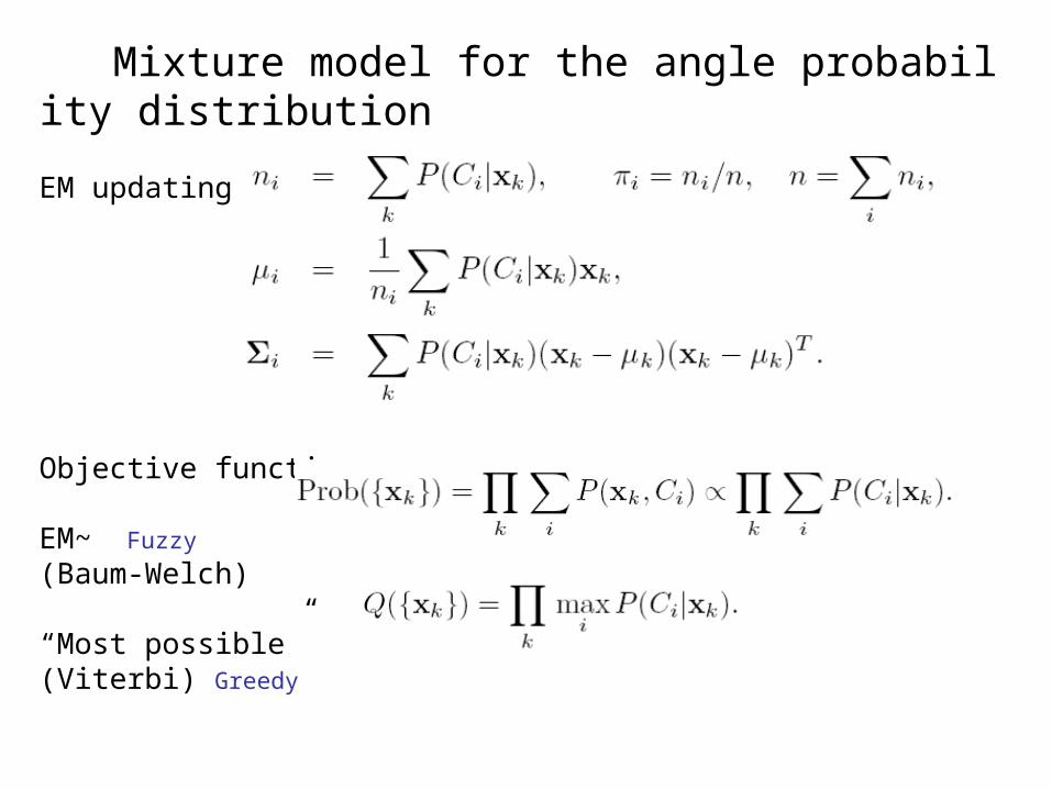
Mixture model for the angle probability distribution
c: the number of the normal distribution categories
Bayes formula:
Fuzzy vs. greedy assignment of structural codes
Mixture model for the angle probability distribution
EM updating
Objective functions
EM~ Fuzzy
(Baum-Welch)
“Most possible”(Viterbi) Greedy

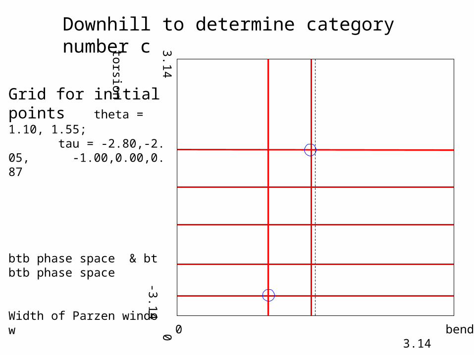
• Downhill search for distribution density peaks Objective function: counts in a box centered at the given point. Grid of initial points (2*5*2 *5*2) Box size (0.1~0.2 radians) ~ Parzon window width ~ resolution• Three-angle space (4-residue unit) vs. five-angle space (5-residue unit) b1t1b2t2b3 ~ b1t1b2 + b2t2b3
• EM traning (fixed category number, approximate category centers)• Tracing the Viterbi likelihood of the ‘most possible’ category states• ‘Good’ centers survive after the training.
3.14 0 -3.14
torsion0 bend 3.14
Grid for initial points theta = 1.10, 1.55; tau = -2.80,-2.05, -1.00,0.00,0.87
btb phase space & btbtb phase space
Width of Parzen window
Downhill to determine category number c

17 structure states from the mixture model

Conformational alphabet and CLESUMConformational letters = discretized states of 3D segmental conformations. A letter = a cluster of combinations of three angles formed by C pseudobonds of four contiguous residues. (obtained by clustering according to the probability distribution.)
Centers of 17 conformational letters

2’ structure and codes
Mutual Information
between
Codes & 2’ structures
= 0.731

Forward transition rates
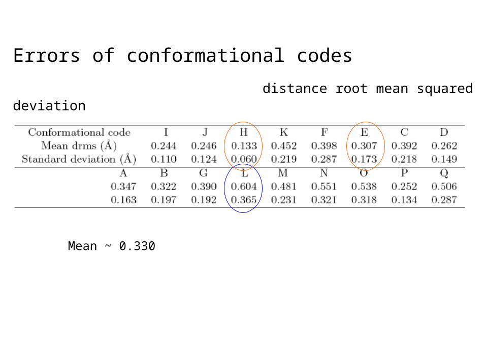
Errors of conformational codes
distance root mean squared deviation
Mean ~ 0.330
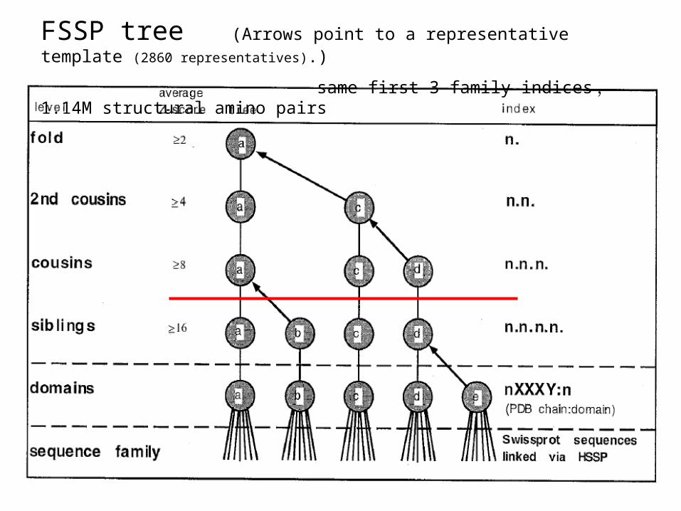
FSSP tree (Arrows point to a representative template (2860 representatives).)
same first 3 family indices , 1.14M structural amino pairs

FSSP representative pairs with the same first three family indices are used to construct CLESUM.
amino acidsa.b.c.u.v.w avpetRPNHTIYINNLNEKIKKDELKKSLHAIFSRFGQILDILVSRS... a.b.c.x.y.z ahLTVKKIFVGGIKEDT....EEHHLRDYFEQYGKIEVIEIMTDRGS
conformational lettersa.b.c.u.v.w CCPMCEALEEEENGCPJGCCIHHHHHHHHIKMJILQEPLDEEEBGAIKa.b.c.x.y.z ...BBEBGEDEENMFNML....FAHHHHHKKMJJLCEBLDEBCECAKK
NAB++; NBA++;

Similarity between conformational letters
CLESUM: Conformational LEtter SUbstitution Matrix
Mij = 20* log 2 (Pij/PiPj) ~ BLOSUM83, H ~ 1.05
constructed using FSSP representatives.
typical helix
typical sheet
evolutionary
+ geometric

1urnA avpetRPNHTIYINNLNEKIKKDELKKSLHAIFSRFGQILDILVSRS... 1ha1b ahLTVKKIFVGGIKEDT....EEHHLRDYFEQYGKIEVIEIMTDRGS1urnA CCPMCEALEEEENGCPJGCCIHHHHHHHHIKMJILQEPLDEEEBGAIK1ha1b ...BBEBGEDEENMFNMLFA....HHHHHKKMJJLCEBLDEBCECAKK
1urnA LKMRGQAFVIFKEVSSATNALRSMqGFPFYDKPMRIQYAKTDSDIIAKM1ha1b GKKRGFAFVTFDDHDSVDKIVIQ.kYHTVNGHNCEVRKAL1urnA ...GNGEDBEEALAJHHHHHHIKKGNGCENOGCCEFECCALCCAHIJH1ha1b AGCPOLEDEEEALBJHHHHI.IJGALEEENOGBFDEECC......... gap panalty: (-12, -4)
Example: FSSP alignment and CLESUM alignment
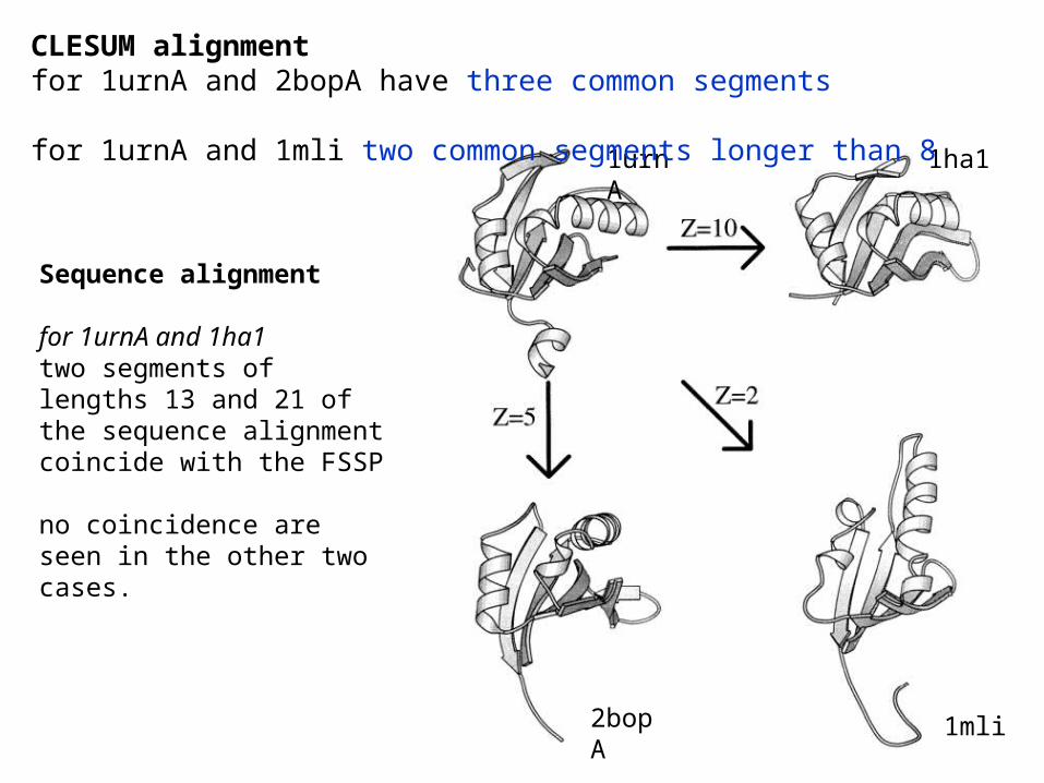
1urnA 1ha1
2bopA 1mli
CLESUM alignment for 1urnA and 2bopA have three common segments for 1urnA and 1mli two common segments longer than 8
Sequence alignment
for 1urnA and 1ha1 two segments of lengths 13 and 21 of the sequence alignment coincide with the FSSP
no coincidence are seen in the other two cases.
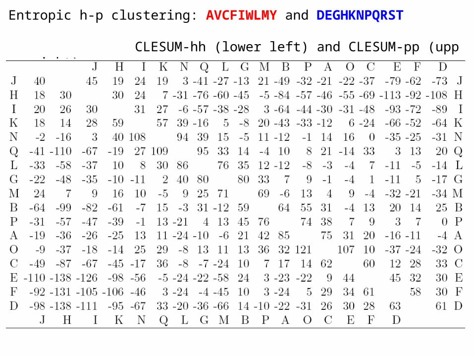
Entropic h-p clustering: AVCFIWLMY and DEGHKNPQRST
CLESUM-hh (lower left) and CLESUM-pp (upper right)
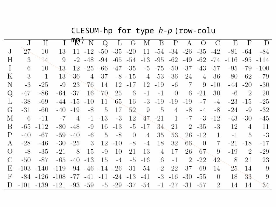
CLESUM-hp for type h-p (row-column)

Fast pair structure alignment
Protein structures comparison: an extremely important problem in structural and evolutional biology.
• detection of local or global structural similarity • prediction of the new protein's function. • structures are better conserved → remote homology detection • Structural comparison → organizing and classifying structures discovering structure patterns discovering correlation between structures & sequences → structure prediction

CLePAPS: Pairwise structure alignmentStructure alignment --- a self-consistent problemCorrespondence Rigid transformation
However, when aligning two protein structures, at the beginning we know neither the transformation nor the correspondence.
DALI, CEVASTSTRUCTAL, ProSup
CLePAPS: Conformational Letters based Pairwise Alignment of Protein Structures
Initialization + iteration• Similar Fragment Pairs (SFPs); • Anchor-based; • Alignment = As many consistent SFPs as possible

Rigid transformation for SuperimpositionFinding the rotation R and the translation T to minimize
If the two sets of points are shifted with their centers of mass at the origin, T=0. Let X3xn any Y3xn be the sets after shift. . Introduce = ,the objective function is defined aswhere Lagrange multipliers are g and symmetric matrix L, representing the conditions for R to be an orthogonal and proper rotation matrix. constraint:
where M is symmetric, and S = diag(si), si = 1 or -1. |C| = |R||M| = |M| = |D||S|.Singular values are non-negative, |D|>0. Finally, |S| = sgn(|C|), and
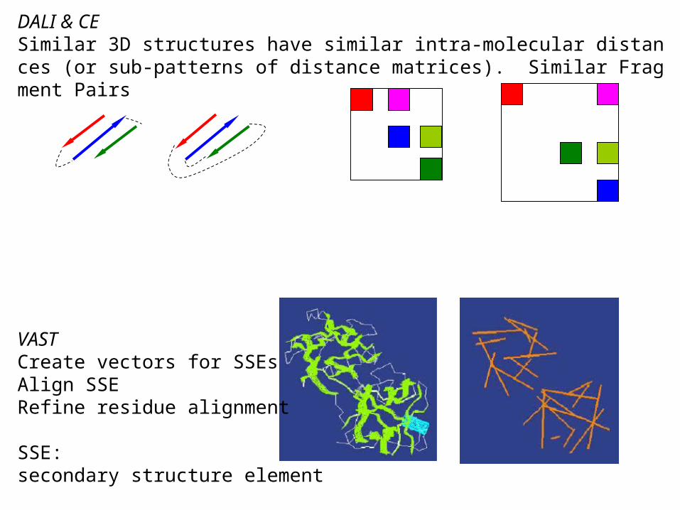
DALI & CESimilar 3D structures have similar intra-molecular distances (or sub-patterns of distance matrices). Similar Fragment Pairs
VASTCreate vectors for SSEsAlign SSE Refine residue alignment
SSE: secondary structure element

Anchor-based superposition
SFPs
anchor SFP
consistent
inconsistent
Collect as many consistent SFPs as possible

the smaller
similar
seed
Redundancy removal
shaved
kept
SFP = highly scored string pair• Fast search for SFPs by string comparison
• CLESUM similarity score importance of SFPs
Guided by CLESUM scores, only the top few SFPs need to be examinedto determine the superposition for alignment, and hence a reliable greedy strategy becomes possible.

rank 1 3 5 2 4
Example: Top K, K = 2; J = 5
Anchor
Anchor
# of consistent SFBs = 4 # of consistent SFBs = 1
Selection of optimal anchor
1
2
Top-1 SFB is globally supported by three other SFPs, while Top-2 SFB is supported only by itself.

Anchor
‘Zoom-in’
d1
d2
d3
d1 > d2 > d3
successively reduced cutoffs for maximal coordinate difference
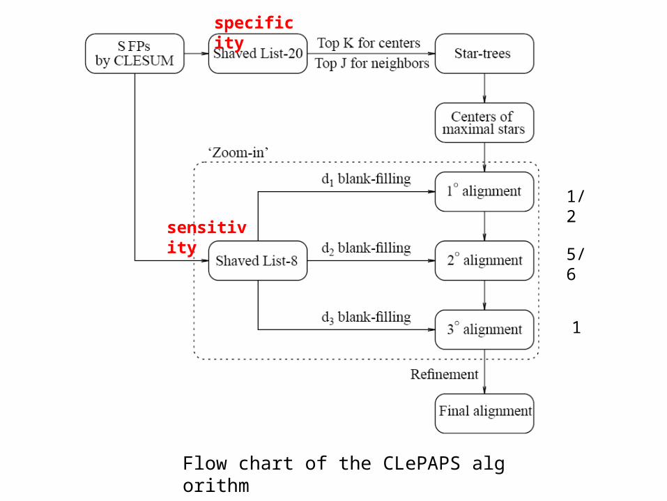
Flow chart of the CLePAPS algorithm
specificity
sensitivity
1/2
5/6
1

• Finding SFPs of high CLESUM similarity scores• The greedy `zoom-in' strategy• Refinement by elongation and shrinking
• The Fischer benchmark test• Database search with CLePAPS• Multiple solutions of alignments: repeats, symmetry, domain move• Non-topological alignment and domain shuffling

Fast Multiple structure alignment
Multiple alignment carries significantly more information than pairwise alignment, and hence is a much more powerful tool for classifying proteins, detecting evolutionary relationship and common structural motifs, and assisting structure/function prediction.
Most existing methods of multiple structural alignment combine a pairwise alignment and some heuristic with a progressive-type layout to merge pairwise alignments into a multiple alignment. like CLUSTAL-W, T-Coffee: MAMMOTH-mult, CE-MC• slow• alignments which are optimal for the whole input set might be missed
A few true multiple alignment tools: MASS, MultiProt

CE-MC: a multiple protein structure alignment server1) CE all-against-all pairwise alignments; 2) guide tree using the UPGMA in terms of Z-scores; 3) progressive alignment by sequentially aligning structures according to the t
ree; 4) highest scoring structure pair between two clusters is used to guide the ali
gnment of the clusters; 5) eligible column in the alignment contains residues (not gaps) in at least on
e-third of its rows. Column distance is defined as geometric distance averaged over residue pairs at each column.
6) Scoring function
M=20, l: total eligible columns; A=0, if di<d0; A=10, if di>d0; gap penalty G=15 (open) -7(extend).
7) Random trial moves are performed on the alignment one residue at a time or one column at a time and a new score is calculated for each trial move.
Maximum number of structures = 25.

Vertical equivalency and horizontal consistencylocal similarity among consistent spatial
structures arrangement for a pair

MultiProt – A Multiple Protein Structural Alignment Algorithmlargest common point (LCP) set detection Multiple LCP: for each r, 2 ≤ r ≤ m, find the k largest -congruent multiple align
ments containing exactly r molecules. Detect structurally similar fragments of maximal length. 0) iteratively choose every molecule to be the pivot one. 1) establish an initial, local correspondence, and the 3-D transformation 2) calculate the global similarity based on some distance measure. a) Multiple Structure Fragment Alignment. (protein, start, width), {p,i,l} b) Global Multiple Alignment. given fragment pair → pairwise correspondenc
e → multiple correspondence → iterative improvement. c) Bio-Core detection. hydrophobic (A,V,I,L,M,C) polar/charged (S,T,P, D,E,K,
R,H,Q,N), aromatic (F,Y,W) glycine (G). Multiple Alignment by Secondary Structures (MASS) two-level alignment using both secondary structure and atomic representation.
SSE assignment SSE representation Local basis alignment Grouping Global extension Filtering and scoringinitial local alignments are obtained based on SSE coarse representation. Ato
mic coordinates are then used to refine and extend the initial alignments and so to obtain global atomic superpositions.
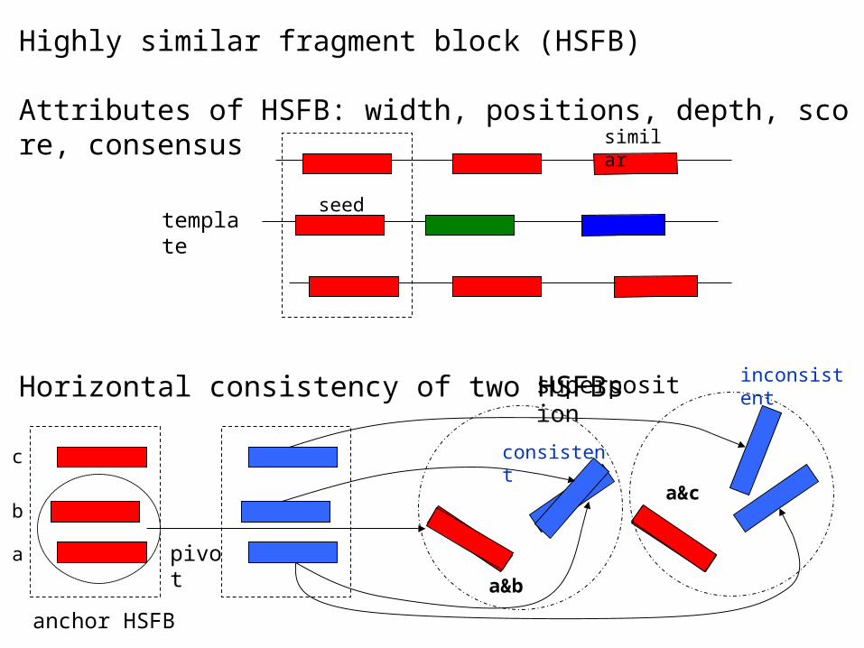
Highly similar fragment block (HSFB)
Attributes of HSFB: width, positions, depth, score, consensus
Horizontal consistency of two HSFBs
template
pivot
superposition inconsistent
consistent
anchor HSFB
similar
seed
a
b
c
a&b
a&c

1. Creating HSFBscreate HSFBs using the shortest protein as a templatesort HSFBs according to depths, then to scoresderive redundancy-removed HFSBs by examining position overlapIf the new HSFB has a high proportion of positions which overlaps with existing HSFBs, remove it.
2. Selecting optimal HSFBfor each HSFB in top K select the pivot protein based on the HSFB consensus;superimpose anchored proteins on the pivot; find consistent HSFBs;A consistent HSFB contains at least 3 consistent SFPs.
select the best HSFB which admits most consistent HSFBs;
3. Building scaffoldbuild a primary scaffold from the consistent HSFBs;update the transformation using the consistent HSFBs;recruit aligned fragments;improve the scaffold;create average template;
4. Dealing with unanchored proteinsUnanchored protein: has no member in the anchor HSFB which is supported by enough number of consistent SFPs.
for each unanchored protein if (members are found in colored HSFBs) find top K members;Try to use ‘colored’ HSFBs other than the anchor HSFB.
else search for fragments similar to the scaffold, and select top K; pairwisely align the protein on the template;
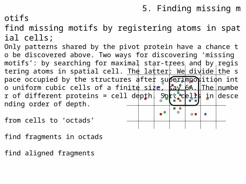
5. Finding missing motifsfind missing motifs by registering atoms in spatial cells;Only patterns shared by the pivot protein have a chance to be discovered above. Two ways for discovering ‘missing motifs’: by searching for maximal star-trees and by registering atoms in spatial cell. The latter: We divide the space occupied by the structures after superimposition into uniform cubic cells of a finite size, say 6A. The number of different proteins = cell depth. Sort cells in descending order of depth.
from cells to ‘octads’
find fragments in octads
find aligned fragments
6. Final refinementrefine the alignment and the average template;

Conclusion
CLePAPS and BLOMAPS distinguish themselves from other existing algorithms for structure alignment in the use of conformational letters. • Conformational alphabet: aptly balance precision with simplicity• CLESUM: a proper measure of similarity between states• fit the -congruent problem • CLESUM extracted from the database FSSP contains information of structure database statistics, which reduces the chance of accidental matching of two irrelevant helices. evolutionary + geometric = specificity gain
For example, two frequent helices are geometrically very similar,
but their score is relatively low.• CLESUM similarity score can be used to sort the importance of SFP/HSFBs for a greedy algorithm. Only the top few SFP/HSFBs need to be examined.
Conclusion
Greedy strategies:HSFBs instead of SFBsUse the shortest protein to generate HSFBUse consensus to select pivotTop K --- guided by scoresOptimal anchor HSFBMissing motifs
Tested on 17 structure datasetsFaster than MASS by 3 orders

The End


![MOTIF XF Editor VST Owner’s Manual7.Sélectionnez « MOTIF XF6 (MOTIF XF7 ou MOTIF XF8) » dans la colonne [FW Device] (Périphérique FW). 8.Sélectionnez « MOTIF XF6 (MOTIF XF7](https://static.fdocuments.net/doc/165x107/611158b13f31404d2d274378/motif-xf-editor-vst-owneras-manual-7slectionnez-motif-xf6-motif-xf7-ou.jpg)