SCHOOL OF ECONOMICS

Discussion Paper 2005-07

Some Recent Evidences about the Global Integration of Chinese Share Markets

Yong Hong, Yan and Bruce Felmingham (University of Tasmania)

ISSN 1443-8593 ISBN 1 86295 289 2

Some Recent Evidences about the Global Integration of Chinese Share Markets

Yong Hong Yan Bruce Felmingham**

School of Economics University of Tasmania

Private Bag 85 Hobart Tasmania 7001

AUSTRALIA

School of Economics University of Tasmania

Private Bag 85 Hobart Tasmania 7001

AUSTRALIA Telephone:0061 3 6226 6336 Facsimile: 0061 3 6226 7587 E-mail: yhyan@utas.edu.au

Telephone:0061 3 6226 2312 Facsimile: 0061 3 6226 7587

E-mail: bruce.felmingham@utas.edu.au

November 2005

* Corresponding Author

Abstract:

First and second order instability tests and cointegration tests are applied to China and other seven market indices and their long run relationship on daily data from January 2 1992 through July 16 2004. First order instability is synonymous with non stationarity and second order instability with structural breaks. The methodologies developed by Perron (1997) and Zivot and Andrews (1992) are employed for unit root tests allowing for structural break while recursive estimation developed by Hansen and Johansen (1993) is applied to test cointegration relationships subject to structural breaks. The structural break identified among eight markets coincides with the Asian crisis period. The increasing strength of cointegrating relationships time (after the late of 2003) reflects the higher extent of economic interdependence among the eight countries following Asian crisis. Continuing upward growing trend with the extended period after 2004 indicates the more difficulties to maintain the benefits from international portfolio diversification. The results in this study also reveal that there exist long-run cointegration relationship between market of China and other countries. Analytical results in this study show China is interactive rather than fairly isolated as reported previously in the literature.

4

1. Introduction

When the government of the People’s Republic of China opted for a strategic change

in 1978, the global economies foresee an emerging market rich in both the diversity and

depth of Chinese markets. Following that benchmark, decisions taken in 1978, foreign direct

investment and experts have flowed into China and the Chinese economy has accommodated

the expansion of foreign imports by achieving almost unprecedented growth rates up to

occurrence of the Asian Currency Crisis in 1997-98, in spite of that hic up, China is back on a

spectacular growth path. However, central to the substance of its current growth is the further

sophistication of PRCs capital markets and the further reform of its currency exchanges and

its share markets. It is this latter component of the capital which is the focus of the following

study.

Our purpose in this paper is briefly stated. It is to determine the extent to which

China’s major share markets are integrated with global share markets. In pursuing this goal,

we take into account evidence of both first and the second order stability of individual share

price indices (SPIs) and of relationship between the time paths of the Chinese SPI with a mix

of foreign SPIs. This distinction between first and second order stability is defined in Yan and

Felmingham (2005) and in general it was reduced to the following interpretation: first order

instability is broadly aligned with the non-stationarility of an individual time series and

second order instability is concerned with structural breaks in individual time series and in

the long term relationships linking China’s SPIs with foreign ones.

For an emerging nation such as China’s it is unlikely that the evolution of a mature

share market will occur without incident or shocks to the system. Included among these

incidents or shocks are the effects wrought by policy intervention, which is the case of an

emerging countries such as China can have quite remarkable effects on the time path of

prices. To accommodate the importance of breaks we conduct test for first and second order

5

instability of the individual time series and test for structural breaks in the long run

relationship between individual SPIs.

The following analysis of SPI integration based around the integration of China’s

Shanghai Composite Index with the Korea Composite Index, the Hong Kong Hang Seng

Index, the Taiwan Weighted Index, the US S&P 500 Composite Index, the Japan Nikkei 225

Index, the Singapore Straits Times Index and the Australian All Ordinary Index.

There are two major Chinese share markets: the Shanghai Composite and the

Shengzhen Composite. Since its establishment in 1990, the Shanghai market has expanded

rapidly in terms of market capitalization, trading volume and the number of firms listed and it

also has a strong contemporaneous relationship with the Shenzhen market through time. Also

we believe the Shanghai market will become predominant in future years. Therefore, we have

opted for the inclusions of the Shanghai Composite over the Shenzhen index.

It is appropriate also to include in our example because of the weight of two target

economies, namely, the US and Japan. The inclusion of the Hang Seng and Taiwan weighted

indices provides an opportunity to test the relationship between these Chinese markets. The

inclusion of the Korea and the Singapore indices accommodate the influence of a major

source of China’s inward FDI (Korea) and one of smaller countries currently negating a

bilateral free trade agreement with the PRC, namely Singapore. Australia too is seeking

dialogue with the PRC for a bilateral agreement so its inclusion is warranted on the same

grounds. From an Australian perspective, China is Australia’s 2nd largest merchandise

import market source behind Japan.

6

2. Data Description

All data are daily closing prices in local currency purchased from global financial

database. The indices included in this study are the China Shanghai Composite Index, the

Korea Composite Index, the Hong Kong Hang Seng Index, the Taiwan Weighted Index, the

US S&P 500 Composite Index, the Japan Nikkei 225 Index, the Singapore Straits Times

Index and the Australian All Ordinary Index. Have mentioned earlier, the choice of countries

is based on the economic ties between these country and China. The sample covers the period

from January 1992 to July 2004 all together 3273 daily observations. This enables us to test

the stability of long-run stock market relationships with respect to major events over time.

While observations are missing because markets were on some days closed, closing prices of

the preceding day are used as a proxy for that day. In order to ensure the same number of

observations, all the observations from Saturday’s trading in Taiwan and Korea are omitted to

ensure that the same number of observations is included for each index.

Literature showed that there is much stronger evidence of cointegration when using

monthly data than when daily data are employed. In order to capture the effect of the

cointegration relationship precisely daily data is used in this study. The starting dates are

determined by the earliest date for which Chinese data are available. Using nominal stock

prices means that the effect of inflation is buried in stock returns. Nevertheless, there is the

non-trivial issue of how to deflate stock prices and the relationship between stock returns and

inflation is quite complex. So we adopt the nominal stock prices in this study. All data are

transformed by taking natural logarithms. The nine share price indices levels and differences

are graphically displayed on Figure 1.

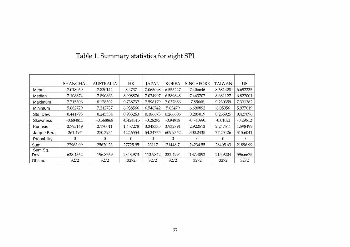
A brief discussion regarding the characteristics of the selected markets is useful. Such

information is supplied on Table 1. Summary statistics are reported for levels calculated as

the log of the price indices. Over the full period, the Hong Kong portfolio has the highest

7

standard deviation. At the other extreme Japan has the lowest standard deviation. The

skewness, excess kurtosis and normality statistics indicate that, overall, the levels showed

significant deviations from normality over the sample period. This is a common feature of

most financial data.

3. Methodologies

Our tests for instability of the price index level are based on Harvey’s (1981)

argument that a non stationary time series are explosive and therefore unstable. Following the

argument of Felmingham and Mansfield (2003), a stationary time series exhibits stable

properties having a time invariant, finite variance while random innovations have a transitory

impact on a stationary series. The series is mean reverting and its autocorrelation function

declines with lag length. So a stationary series is stable in this context. We deem the two

series studied in this paper to be stable if they are stationary and label this first order stability.

However, stability of price level does not rest on the stationarity issue alone. We also test the

eight share price indices for structural breaks. It is one thing to have a smooth, stationary and

therefore stable series; it is another altogether to have a series which is stable subject to a

structural break in that series. This second order test for instability involves some basic

questions as to the causes of the break.

Similarly with price indices levels, the long term relationship between variables based

on Johansen cointegration test which suffers the influences of structural breaks in the data set.

We test for the presence of second order stability of long term relationship between Chinese

and other seven markets by firstly obtaining the results of long run relationship from a

standard cointegration test and then we exam the instability of this long term equilibrium

relationship. Whether this relationship between the countries keeps constant during all sample

period without any outside influences is our focus. This second order instability test for a

8

long-run relationship based on the recursive estimation method suggested by Hansen and

Johansen (1993) explained later.

3.1 Unit Root Tests (the first and second order instability test of individual price index time series) A necessary but not sufficient condition for cointegration is that each of the variables

involved in a study should be nonstationary in levels but stationary in first differences. Perron

(1989) argues that if there is a break in a deterministic trend, then traditional Augmented

Dicker Fuller unit root tests will lead to a misleading conclusion to the effect that there is a

unit root, even if there is not. For each of the variables first order instability is synonymous

with non stationarity and second order instability with structural breaks. Perron (1997) and

Zivot and Andrews (1992) indicate that the date of any structural break point in a time series

should be endogenously determined. In the following analysis, the null hypothesis of a unit

root without an exogenous structural break is tested against the alternative that the series is

trend-stationary with a one-time break. Perron’s (1997) structural break test requires the

estimation of the following regression:

t

it

k

iittBttt ycyTDDTtDUy εαδγβθµ +∆++++++=

−=− ∑

11)(

(1)

Where 1tDU = if ( ), if and 1 if 1B t B B B Bt T DT t T t T D T t T> = − > = = + . BT denotes the time

at which a structural break occurs. We will select the breakpoint using the minimum t-

statistic for testing the null hypothesis of a unit root (a = 1).

The structural break tests developed by Zivot and Andrews (1992) involve the

following regressions:

t

it

k

iitttt ycyDTtDUy εαγβθµ +∆+++++=

−=− ∑

11

*

(2)

9

Where 1 if ,0BDUt t T= > otherwise if ,0t B BDT t T t T∗ = − > otherwise. The break point is

chosen as the value which minimizes the t-statistic for testing the null hypothesis of a unit

root (a = 1). Unlike Perron (1997), the one-time break dummy, ( )BD T , is not included in

Zivot and Andrews (1992) model. In equation (2), we estimate Zivot and Andrews’ model

which allows for a break in both intercept and trend of a time series. The testing procedure in

Zivot and Andrews (1992) is similar to that of Perron (1997) described above. Perron (1997)

simulates critical values for a finite sample size which are quite different from the asymptotic

critical value derived by Zivot and Andrews.

3.2 Cointegration Analysis

After the individual series are found to be non-stationary and are integrated of the

same order*, cointegration analysis is used to determine whether the index series become

stationary in a linear combination. For example, two variables are cointegrated when a linear

combination of these two variables is stationary, even though each may individually be non-

stationary. So these two variables can be said to have a long run relationship. The

cointegration test is performed using the Johansen (1991) method and involved error

correction term.

3.2.1 Johansen’s Cointegration Estimation (the first order instability test of long run relationships)

Similarly, the first and second order stability is considered when investigating long

run relationship. The first order stability test of long run relationships is cointegrated

relationship among variables without structural breaks considered and the second order

stability does take the breaks account.

10

Johansen (1991) demonstrate that the procedure involves the identification of the rank

of Π in the following specification:

∆ tx =ζ + ∑−=

=−∆Γ

1

1

ki

iiti x + Π 1−tx +μ (3)

where, Γ and Π represent coefficient matrices, ∆ is a difference operator. If Π has zero rank,

no stationary linear combination can be identified. In other words, the variables in tx are

noncointegrated. If the rank r of Π is greater than zero, however, there will exist r possible

stationary linear combinations. The parameter Π may be decomposed into two matrices α and

β, (each m ×r) such that Π = αβ′. In this representation β contains the coefficients of the r

distinct cointegration vectors that render β′ tx stationary, even though tx is itself non-

stationary and β′ tx which is called the error correction term. Further, α is the speed-of-

adjustment coefficient of the error correction term and measures the average speed of

convergence of the series in question towards the long-run equilibrium. If α equal zero, then

this series does not participate in the adjustment back towards equilibrium and is described as

being weakly exogenous.

Additional testing of β, the coefficients of the cointegration vectors, can produce

further information on long-run market linkages. We are interested in how many markets are

excluded in all of the identified long-run relationships. This hypothesis can be tested by

examining whether each coefficient is equivalent to zero. In order to test this proposition for

each of the equity markets entering the cointegration vector significantly, we test for zero

restrictions upon each of the coefficients derived by the Johansen procedure.

Applications of the Johansen procedure are quite popular in a multivariate context. As

Masih and Masih (1995) point out, the results of the Johansen statistic in bivariate studies

11

have also been shown to be more robust than those from the Engle-Granger approach. So we

adopt the Johansen procedure for both bivariate and multivariate analysis at a later analysis.

3.1.2.2 Structural Break Tests (the second order instability test in long run relationships) Recent studies in particular (Elyasiani and Kocagil (2001)) have shown that

Johansen’s test suffers from temporal instability. An implicit assumption underlying these

tests is that news and particular events do not significantly affect the stability of this system

in terms of altering the number of common stochastic trends. This makes it necessary to carry

out the second order stability test in order to get full information of cointegration relationship.

To tackle this problem Hansen and Johansen(1993) have suggested some methods for the

evaluation of parameter constancy in cointegrated VAR models to identify the structural

breaks which changing the number of cointegration vectors.

In contrast to the previous studies cited above, recursive diagnostic techniques are

performed to ensure the robustness of the results from the conventional Johansen tests and to

examine the stability of the cointegration relationship.

There are three methods to evaluate the parameter constancy in cointegrated VAR

models.

The first test is called the Rank test. This is accomplished by first estimating the

model over the full sample, and the residuals corresponding to each recursive subsample are

used to form the standard sample moment. The obtained sequence of trace statistics is scaled

by the corresponding critical values.

Recall from earlier section that the Trace test is calculated in the following equation:

( ) ( )1ln 1

p

trace ii r

r Tλ λ= +

= − −∑

12

When determining the number of cointegration vectors, sequential testing is used. Firstly, the

null hypothesis of r = 0 is tested against the alternative of r = p (the null of all series being

unit root series against the alternative hypotheses of all series being stationary series):

( )0H r r p≤ = . If this test is rejected, the null hypothesis of at most one cointegration

vector, r < = 1, is tested against the alternative hypothesis of r = p: ( )1H r r p≤ = . And so

on until the hypothesis of r < = p - 1 is tested against r = p: ( )1H r p r p≤ − = . When a

particular hypothesis cannot be rejected, the sequential testing procedure is truncated.

Therefore, if the cointegration rank is constant throughout the sample period (no

significant change of the rank), all recursive test statistics for the Trace hypotheses should

exceed the critical test values and be upward sloping.

A second test deals with the null hypothesis of the constancy of the beta for a given

cointegration rank. Hansen and Johansen propose a likelihood ratio test that is constructed by

comparing the likelihood function from each recursive subsample with the likelihood

function computed under the restriction that the cointegrating vectors estimated from the full

sample falls within the space spanned from the estimated vectors of each individual sample.

The test statistic is a chi-square distributed with (p - r)r degrees of freedom, where p stands

for the number of endogenous variables and r for the cointegration rank.

The final test examines the constancy of the individual elements of the cointegrating

vectors. When the cointegration rank is greater than one the elements of the vectors can not

be identified unless certain restrictions are imposed. However there is a unique relationship

between the eigenvalues and the cointegrating vectors. Therefore the structural change will

be reflected in the estimated eigenvalues when these vectors have undergone a structural

change.

13

3.3 Granger Causality Tests

In order to examine the predictive abilities of different time series in the model, a

Granger causality test will be applied after cointegration method is used. It allows the

framework to test for the presence of unidirectional causality and bi-directional causality

which can give more information about the short term relationship in comparison with

cointegration analysis. Pairwise Granger (1969) causality tests are carried out to test whether

an endogenous variable can be treated as exogenous. To implement the Granger test, we

estimate the reduced form of VAR equation the reduced form of VAR equation by equation

as follows:

titk

i iitk

i it uXbYaY ++= −=−= ∑∑ 11

X and Y are stock market index levels. The Granger test regresses index Y on lagged index Y

and lagged index X. The Granger F-statistic tests the null hypothesis that index X does not

Granger cause or predict index Y in above equation. The null is rejected if the coefficients ib ,

are significantly different from zero. Then we can conclude that the lagged right-hand side

variable has significant linear predictive power (granger-cause) for the left-hand side

variable. The estimation of the VAR model requires the variables to be unit root free and

non-cointegrated.

4. Empirical Results

4.1 Unit Root Tests Results (the first and second order instability test of price indices level)

In addition to the Zivot and Andrews (1992) test over the full sample, we also subject

each index to an Augmented Dickey-Fuller (ADF) unit root test for the first and second order

stability of share price indices. The relevant test statistics for the ADF, Zivot and Andrews

(1992) analyses of stationarity for each share price index are shown on Table 2.

14

From the ADF tests on Table 2, it is clear that the null hypothesis of a unit root in all

prices in levels at the 1 percent level of significance cannot be rejected. However, the

Shanghai series is exceptionally significant at the 5 percent level. These results

overwhelmingly support the suggestion that stock prices are non-stationary processes in

levels. This finding is consistent with the finds of Kasa (1992) and Blackman et al (1994) that

equity market prices, in general, contain a unit root in their levels form. ADF unit root tests,

using the first difference of each series, were also conducted to test for higher orders of

integration. None of these tests for higher order integration reject the null hypothesis that all

share market price indices are I(1) at the one percent level of significance. Overall, the unit

root tests do not indicate any significant evidence to reject the hypothesis that all indices are

I(1).

The results of Zivot and Andrews tests are reported on Table 2 and suggest that all

stock series are non-stationary allowing for a break in the level and trend of the time series

except for the Shanghai market at the 5 percent significance level. According to estimated

test statistics based on Zivot and Andrews test, the break points occurred during sample

period in the most time series are supported by visual inspection of the graphs shown on

Figure 1.

The unit root test results shown on Table 2 indicate that most stock indices are

integrated of order one suggesting that the analysis should proceed to cointegration and error

correction model tests of long-run relationships between share price movements.

4.2 Bivariate Cointegration Test (The first and second order instability test of long run relationship) The unit root test statistics reveal that each series is nonstationary in log levels but

stationary in log first differences. Given the common properties of the share price indices, all

indices are stationary after applying differencing only once, like many macroeconomic

15

variables. The relationships between Chinese markets with other international share markets

are initially investigated using bivariate techniques. As mentioned in previous chapter,

Shanghai series representative Chinese markets. There will be seven different individual

pairings, and therefore seven VAR models.

The Johansen bivariate cointegration test is used to obtain the rank of the

cointegration vector after the lag length is identified via LR tests. An intercept and no trend

are specified for the cointegration equation. Eigenvalues and corresponding trace and

maximum-eigenvalue statistics are detailed on Table 3.

The test statistics on Table 3 for the bivariate relationship between China and four

other markets: Hong Kong, Korea, Australia and the US are significant according to the

critical values provided by Johansen Nielsen(1993). This implies that there are long-term

cointegration relations existing between the Shanghai market and markets in Hong Kong,

Korea, Australia and the US. However, the relationships involving China and the remaining

markets are not cointegrated.

Diagnostic tests were undertaken to check the residuals for all indices and the results

of these tests are shown on Table 4. The critical values of the Johansen cointegration test on

Table 3 were conducted subject to the assumption of normal innovations (the error terms of

time series have constant variance and the correlation between error terms does not change

over time). Therefore, deviations from assumption properties affect the results adversely. It is

necessary to test whether the assumptions are sustainable or not in this case studied.

On Table 4, LM tests for first and fourth order autocorrelation do not indicate its

presence in the residuals for the models and suggest that the lag length in each model has

captured serial correlation effectively. The test of normality is based on a multivariate version

of the univariate Shenton-Bowman test, see Doornik & Hansen (1994). This confirms the

results of the Jaque-Bera test shown on Table 1.

16

4.3 Granger Causality Analysis

In Table 2 and Table 3 we reported unit root and bivariate cointegration test. As can

be seen all variables are stationary and three pairs of variable are not cointegrated. This made

the causality analysis possible to find out the predictability of each price index particularly if

the Shanghai index has a significant effect on other international price indices (Taiwan,

Singapore and Japan) or if these international price indices have a significant effect on

Shanghai price index we are interested in this study.

It clearly shows from Table 5 that causality from the Shanghai index to every other

three remaining indices are not significant during the whole sample period. Interesting

findings of linkage here are that the changes of every other market index are strong Granger-

cause change of Shanghai market. The strong form of causality is evident running from

Taiwan to Shanghai. The causal influence of the Singapore market on Shanghai market is

also obviously observed even it is not strong as the causality from Taiwan. In addition, Japan

market change Granger-cause change of Shanghai market at the highest significant level in

comparison with Taiwan and Singapore.

4.4 Multivariate Cointegration Analysis Results

The bivariate analysis completed in the previous section cannot reveal the full extent

of the long run relationships existing among the full set of share price indices. We require a

multivariate cointegration analysis to achieve this purpose. The results from this multivariate

study will indicate the number of cointegration vectors present and if the number of these is

equal to the number of individual series (8 series in this case), then the eight share market are

perfectly integrated: see Cooray and Felmingham (2004). If these markets are perfectly

cointegrated then there is an apparent opportunity for share market investors to diversify

17

away systemic risks, so the information provided by the multivariate analysis will provide

important information for the international investors.

Results of the rank test for multivariate variables appear on Table 6. The maximal

eigenvalues shown on Table 6 suggests that there is at most a single cointegration vector or

analogously seven independent common stochastic trends within this eight-variable system.

But the trace test statistic indicates two cointegration relationships in this system of eight

markets, meaning these markets share six common trends over the sample period.

The Johansen cointegration test is applied based on the normal innovations of the

vector autogressive model (the error terms of time series have constant variance and the

correlation between error terms does not change over time). Therefore, violations from

assumption properties influence the results adversely. So diagnostic tests are required to

check the characteristics of the residuals in the multivariate case as well. The results are

presented on Table 7. The LM statistic indicates that the optimal lag structure has captured

serial correlation adequately. Non-normality and heteroskedasticity are statistically

significant as they are in the bivariate case.

4.5 Cointegrating Vector Parameter’s Constancy Test (the second order test for instability of long run relationship)

The number of cointegrating vectors resulted from above section is based on the

assumption that the number of cointegrating vectors is fixed and the speed-of-adjustment

coefficient of the error correction term (α) is constant over all sample periods. If the number

of cointegrating vectors in the economic system changes over time because structural break

occurs in the sample period, the rank will vary consequently. Both long-term and short-run

coefficients in the Error-correction model may change as well. Accordingly the chance of

conflicting trace and max eigenvalue statistics results will increase. In this case the Trace

18

Statistic 127.28 rejects the null hypothesis that there is one cointegration relation but max

eigenvalue 41.82 is not significant enough to reject the null hypothesis.

This conflict may be explained by structural breaks which determine second order

instability of long run relationship. This problem can be resolved by conducting diagnostic

test advocated by Hansen and Johansen (1993) to ensure the robustness of the test results and

the reliability of subsequent inferences. A structural break occurring in the sample period can

be captured by recursive cointegration tests presented in Graph 3,4 and 5, 6 regard for rank

test, cointegration vector test and individual elements of cointegration vectors test

respectively.

On Graph 3, the recursive trace statistics are normalized using their 10% critical

values such that the values exceeding 1 indicate statistical significance at the 10% level,

while the number of lines above 1 are the number of cointegrating vectors observed plotted

against time.* In this case, a two-year period between 1992:1:02 and 1994:7:18 is used as the

initial estimation period. The plots of the recursive trace statistics over the period 1994:7:19

through 2004:7:16 are shown on Graph 3. The upper line in the graphs show the path of tests

for ( )0 8H r r≤ = and the lower line in the graph shows the path of tests for

( )7 8H r r≤ = . The first cointegrating vector is statistically significant indicating that eight

time series are linked together by one cointegration vector and according driven by seven

common stochastic trends. However the significant of second cointegration vector after 2003

show that this group are linked together by two cointegration vectors. On the other hand, the

third cointegrating vector emerging after approximately year 2004 to become statistically

significant need more time to be proved as one of the vectors joining markets together. In the

common trends framework such findings are to be interpreted as signs of increased

convergence as the data generating process is then characterized by an increasing number of

cointegration vectors and correspondingly that the share price series are increasingly driven

19

by the same relatively few shocks with a permanent effect (Jesper Rangvid, 2001). So we

draw the conclusion that a system consisting of eight non-stationary time series is driven by

six common stochastic trends and linked together by two cointegration vector. However we

need to note here that all of the cointegrating vectors are upward sloping after late 2003 and

the values of the recursive trace statistics continue to increase hereafter. There seems to be a

tendency for fewer and fewer stochastic trends to drive the whole system as the sample

period is extended. So we could say that these eight markets have become increasingly

convergent over time.

Graph 4 shows Hansen-Johensen (1993) recursive analysis tests result for stability of

the parameter of cointegration vector, beta, giving one cointegration vector. �The test

statistic has been scaled by the normalized using their 5% critical values such that the values

exceeding 1 indicate statistical significance at the 5% level, while the line above 1 means the

inconstancy of beta. The numbers in vertical axis show chi-square value. The test statistic is a

chi-square distributed with (p – r)r degrees of freedom, where p, 8 stands for the number of

endogenous variables and r, 1 for the cointegration rank. Rejection of the null hypothesis in

the middle of 1998 indicates rejection of parameter constancy. In other words, there is

evidence of temporal instability in the long run. Additionally the results suggested that there

is break in the cointegrating vector which is identified as 7th September 1998 which

coincides with the outbreak of Asian crisis. These results confirm the conclusions of Meric

and Meric (1997) (and other researchers) that there is a long-term persistent rise in the co-

movement of equity markets following the Asian crisis. These breaks are partially supported

by visual inspection of graph 1 in terms of slumping indices at the time of Asian Crisis.

However these break points confute the breaks found in the unit root test(see Table 1)

confirming the fact that the single individual time series breaks are not necessary same with

the combination of number of time series.

20

In order to get an appropriate reference of impact of structural break on cointegration

number, we also test the stability of the parameter of cointegration vector when there are two

cointegration vectors. The results shown on Graph 5 clearly indicate that there is no evidence

of temporal instability in the long run giving two cointegration vectors.

Finally with the last test, Graph 6 shows the time paths of the non-zero eigenvalues

with 95% confidence bands giving two cointegration vectors. We get strong support favour of

the constancy of the cointegration vector since the path of the respective Eigenvalue didn’t

present any break point. However it is observed that some observations-especially in the

period around 1998-have a large impact on the parameter estimates.

Hence, based on the overall evidence of the three tests we argue that the estimated

cointegrating vector does display instabilities in recursive estimation.

4.6 Exclusion Test

Giving two cointegration vectors among 8 market indices from the preceding

analyses, a test of whether cointegration is achieved through the adjustment of all indices

proceeds according to the method described above. Zero restrictions are placed upon each of

the coefficients of cointegrating vector in Johansen’s procedure and the results are shown on

Table 8.

The likelihood ratio tests indicate that all these restrictions are rejected except or the

Shanghai and US market and further indicate that the Shanghai and US share indices can be

individually excluded from the cointegrating vectors at the .05 level. This implies that all of

the markets enter the cointegrating vector at a statistically significant level except for the

Shanghai and S&P 500 Composite Index. In general, these results indicate that most markets

adjust in a significant fashion to clear any short run disequilibrium. In addition the largest

coefficient is related to the Singapore index followed by the coefficient for Hong Kong, while

21

the smallest coefficient is the US index indicating that Singapore and HK react quickly to

adjust towards a long run relationship in this eight-country system.

Based on the likelihood ratio test statistics above, the null hypothesis that the

Shanghai and US stock indices are not part of the equilibrium relations cannot be rejected at

the 0.05 level across all possible vector relationships, suggesting that the VAR be

reconstructed without these two indices. So the Johansen cointegration test is conducted

again using six variables in the VAR system without the Shanghai and US markets. This

revised cointegration results appear on Table 9 indicating that there is one long run

relationship based on both trace and max eigenvalue statistics. The comparative results from

the eight-country system and six-country system without Shanghai and US suggest that there

exists a geographical separation between of US and Asia Pacific markets. Additionally,

China’s share market here appears to be relatively isolated from most world markets which

will be also tested in later analysis.

4.7 Exogeneity Test

Following the result that the Shanghai and US market do not enter the long run

relationship as identified by the exclusion test, a further test of the role of speed adjustment

parameter is carried out to find out which index not responsive to disequilibria and form one

of the p - r common stochastic trends.

Based on the present two cointegrating vectors among all eight indices, there must be

6 common stochastic trends. The null hypothesis that the stock indices of Shanghai, Taiwan,

Korea, Australia and Japan are individually weakly exogenous cannot be rejected at the .05

level. Each of them is irresponsive to disequilibria and is one of the (p-r) common stochastic

trends.

22

So we infer from these weak exogenity test results that any of these countries, namely,

Shanghai, Taiwan, Korea, Australia and Japan do not display any short term adjustment to

equilibrium. However, Taiwan, Korea, Australia and Japan do have a long run, but not a

significant short run relationship.

Combined with our earlier exclusion test results which show that the Shanghai market

does not share linkages with other markets through an error-correction channel of causality,

we can draw the conclusion that the Shanghai market does not exert a significant influence on

other markets in the short as well as the long run.

For other markets, particularly, not significantly weakly exogenous ones, they do not

adjust to clear short run equilibria although they are form part of the error correlation process.

We still cannot assume that all five of these markets(Shanghai, Taiwan, Korea,

Australia and Japan) which are not statistically significant in exogenous tests are non-causal

and totally exogenous because the short-run channels via the coefficient of difference of

variable ( Γ in equation (2)) are still active.

The significance of US market indicates that it seems the most likely link to other

markets via short-term channels even if does not involve the long run relationship of system

of an eight share price indices.

The above results are drawn from equation 3 defined as model 1 which allows a

deterministic trend in the level but not in the cointegration relations. In order to get accurate

inferences from the coefficient in the models allowing different specifications of the

deterministic components, another two models arising from restriction on the deterministic

components are also needed to be investigated. The model allowing intercepts in the

cointegration relations is referred model 2. The model allowing a deterministic trend in the

level as well as in the cointegration relations is defined as model 3.

23

Calculated eigenvalues, the trace test and the corresponding critical values under each

model specifications are listed on Table 11. These results can be used to determine if a trend

in the cointegration relations is included and whether this including affects our rank selection

greatly. It is clearly shown in Table 11 that all the statistics are consistent in these three

models with different specifications suggesting that the rank test is not sensitive to the

deterministic components included.

5. Implications

Whether these eight markets converge or not is an important question since portfolio

investment strategies will depend on the degree of integration of these financial markets.

Multivariate cointegration results show that the Chinese markets are cointegrated in the

system. However, market exclusion tests indicate that Chinese market is indeed minimally

integrated with world markets, offering substantial potential for risk reduction in the

Shanghai market.

Exposure to the Australia and US markets do not appear to provide substantial

diversification benefits opportunity for Chinese investors in the long term.

Common trend between the markets of China and Hong Kong does not surprise

because of the increasingly close relationship in trade and politics particularly after 1997

when Hong Kong returned to China. Yong Miao Hong (2003) finds that there exists

significant risk spillovers between Shares B (the share designed for foreign investors trading

in foreign currencies) and the market in Hong Kong. In fact, a strong relationship between

Share B and international markets is expected because B Shares are more sensitive to the

fluctuations of foreign markets. This issue is beyond our scope in this study and will not be

discussed further.

24

Singapore and Korea, two newly industrialized markets in East Asia, have different

ties with the Shanghai market. Stronger common trend between Shanghai and Korea exist in

comparison with the common trend between Shanghai and Singapore. This may be due to the

stronger economics link between China and Korea. China has become the third largest

trading partner of Korea at the end of 2002, while Korea’s total direct investment in China

constitutes about one third of Korea’s total outward foreign direct investment. Economic ties

reinforce the relationship between the two share markets.

The lack of cointegration between the Shanghai and other markets in the group

suggest that the Shanghai market is an attractive market for achieving international

diversification. They should balance their long-run investment on the markets of Taiwan,

Singapore and Japan compared with those of Hong Kong, Korea, Australia and US.

It is interesting to determine if there is a cointegration relationship between China and

the US or Japan. Since Japan is a major investor and trading partner of China, a share market

relationship with Japan may exist. Similarly, because of its economic influence and market

size, the US impact on China’s market could be expected. From the results of the bivariate

cointegration, China’s share market does not share a common trend with Japan in the share

market. Instead, the bivariate cointegration test is strongly statistically leading to the rejection

of the significant to against the null hypnosis that there are no cointegration vectors between

China’s share market and US share market. So basically, it could be said that Chinese market

belongs to the markets those which are moved with US. The fact that the Japan market is not

cointegrated with the Chinese market doesn’t mean the Japan market lost its interests to

investors. Instead, Japan market is still attractive to Chinese investors because of its size and

liquidity. So compared with Japan, US market is more likely to affect Chinese market.

It should be noted in addition that Chinese companies are allowed to go beyond

traditional domestic equity-financing channels to raise capital by listing in overseas capital

25

markets such as the Hong Kong and New York stock exchanges. The existence of foreign

listing shares in these two markets certainty reinforces their long run equilibrium

relationships with China’s share market.

The structural break identified among eight markets coincides with the Asian crisis

period. The increasing strength of cointegration relationships time (after the late of 2003)

reflects the higher extent of economic interdependence among the eight countries following

Asian crisis. Continuing upward growing trend with the extended period after 2004 indicates

the more difficulties to maintain the benefits from international portfolio diversification. The

results in this study consistent with the conclusions of Sorin and Burton (2001) that the co-

movement of global equity markets increase after the Asian Crisis.

Also it is noticed that all the stock markets except Shanghai and US enter the long run

relationship suggesting that there may exists a geographical separation between the US and

Asia-Pacific markets. Additionally, china’s share market is relatively isolated from most

world markets in the long run.

The stock indices of Shanghai, Taiwan, Korea, Australia and Japan are individually

weakly exogenous and each of them is irresponsive to disequilibria. Therefore these five

countries offer good investment diversify in the short run.

It is true that segmented financial markets present greater opportunities for investors

to improve their risk-adjusted returns in comparison with integrated financial markets.

However, investors diversifying their portfolios internationally may earn a higher rate of

return for any given level of risk than they could achieve by holding a purely domestic

portfolio. Some investment barriers such as restrictions on capital movements have made it

hard to fully realise the benefits of diversification. No wonder there is still strong home

country bias that investor still hold a substantial domestic assets portion as explained by

Tesar and Werner (1995). Tesar and Werner use data on international financial transactions

26

across five OECD countries including the US,UK, Canada, Germany and Japan and find

evidence of a home bias in portfolio compositions for investors in all the five countries they

examine. While investors have increased their holdings of foreign stocks in recent years, the

fraction of the portfolio invested abroad remains far less than the share implied by standard

models of optimal portfolio choice. Particularly, when foreign investors facing Chinese stock

markets, the problems with international diversification like currency risk, information costs,

controls to the free flow of capital and political risk need to be considered seriously as well as

portfolio returns.

Therefore, two factors were seen as driving foreign investment toward emerging

markets. One is investor’s desire for portfolio diversification and higher profits. Another is

macroeconomic and structural reform in developing countries. Sensible investors prefer for

countries with sound policies. Stringent capital controls and lack of convertible currency

make Chinese market not favourable to some investors who pursue low risk in the markets.

Such investors wait for further reforms of China’s economy such as freeing up A Shares

market to foreign investors. The history of stock markets’ development in the world shows

that financial market liberalization particularly the relaxation of rules constraining foreign

investors contributed greatly to the surge of stock market. So the openness of Chinese stock

market to the foreign investors is a biggest challenge for maintaining the continuous high

speed growth of stock markets. The empirical evidence suggests that rapid development in

the Chinese share markets has succeed over the past few years, but it is acknowledged that

China’s share market is not as developed and open as some other international markets. On

the other hand, investors who are willing to accept higher risk in search of high return will

favour the China’s share markets.

27

*note: Due to some technical limitations, the software we use(CATS in RATS 6.0) only

produces plots of trace test statistics using built-in 10 percent critical values. However, the

use of the 5 percent significance level does not change the inference reported below.

28

References

Baillie, R. T. and T. Bollerslev (1989). "The Message in Daily Exchange Rates: A Conditional-Variance Tale." Journal of Business and Economic Statistics, (7).

Cheung, Y. and K. S. Lai (1993). "Finite-sample Sizes of Johansen's Likelihood Ratio Tests for Cointegration." Oxford Bulletin of Economics and Statistics.

Cooray, B. F. A. A. (2004). "Parametric and Non-Parametric Tests for RIP Among the G7 Nations", University of Tasmania, School of Economics Discussion Paper 2004-01.

Corhay, A., Tourani Rad, A. and Urbain, J. P. (1992). "GARCH and Cointegration Models for Europen Stock Markets", proceedings of the Third ITFA Meeting: Chapter 3.

Doornik, J. A., and Hansen, H. (1994). "A Practical Test for Univariate and Multivariate Normality", Discussion Paper.

Dwyer, J., Gerald P. and M. S. Wallace (1992). "Cointegration and Market Efficiency." Journal of International Money and Finance, 11(4): 318-327.

Elyasiani, E. and A. E. Kocagil (2001). "Interdependence and Dynamics in Currency Futures Markets: A Multivariate Analysis of Intraday Data", Journal of Banking & Finance 25(6): 1161-1186.

Eun, C. S. and S. Shim "International Transmission of Stock Market Movements", Journal of Financial and Quantitative Analysis, 24(2): 241.

Felmingham, B. A. M. P. (2002). "A Note on the Stability of Real Interest Rates in Australia", International Review of Economics and Finance, 12: 517-24.

Felmingham, B. L, S.S. (2003). "The Stationarity of Australian Real Interest Rates with and without Structural Breaks", Applied Economics Letters, 10: 239-241.

Hansen, H. and S. Johansen (1999). "Some Tests for Parameter Constancy in Cointegrated VAR-models", The Econometrics Journal, 2: 306-333.

Harvey, A. C. (1981). The Econometric Analysis of Time Series, Philip Allen, Oxford.

Johansen, S. E. R. and K. Juselius (1992). "Testing Structural Hypotheses in a Multivariate Cointegration Analysis of the PPP and the UIP for UK", Journal of Econometrics, 53(1-3): 211-244.

Kasa, K. "Common Stochastic Trends in International Stock Markets", Journal of Monetary Economics, 29(1): 95.

Lai, K. S. and M. Lai "A Cointegration Test for Market Efficiency", The Journal of Futures Markets, 11(5): 567.

Meric, I. A. M., J. (2001). "Co-movements of US and Latin American Equity Markets before and after the 1987 Crash", International Review of Financial Analysis.

Nelson, C. R. A. P., C. I. (1982). "Trends and Random Walks in Macroeconomic Time Series", Journal of Monetary Economics, 10: 139-62.

Nunes, L. C., Newbold, P. and Chung, M. K. (1997). "Testing for Unit Roots with Breaks: Evidence on the Great Crash and the Unit Root Hypothesis Reconsidered." Oxford Bulletin of Economics and Statistics, 59(4): 435-448.

Perron, P. (1997). "The Great Crash, the Oil Price Shock, and the Unit Root Hypothesis." Econometrica, 57(6): 1361.

29

Richards, A. J. (1995). "Co-movements in National Stock Market Returns: Evidence of Predictability, but not Cointegration." Journal of Monetary Economics, 36(3): 631-654.

Blackman, S.C., K. H. A. W. A. T. (1994). "Long-Term Relationships between International Share Prices." Applied Financial Economics, 4(4).

Solnik, B. (1974). "Why not Diversity internationally?" Financial Analyst Journal, 20: 48-54.

Tesar, L. A. W., I. M. (1995). "Home Bias and High Turnover." Journal of International Money and Finance, 14: 467-492.

Xiangmei Fan, Y. W, and N. Groenewold (2004). “The Chinese Stock Market: Development and Prospects”, Discussion Paper.

Yin-Wong Cheung, K. S. L. (1998). "Macroeconomic Determinants of Long-term Stock Market Co-movements Among Major EMS Countries." Applied Financial Economics, 9(1).

Zivot, E. and D. W. K. Andrews (1992). "Further Evidence on the Great Crash, the Oil-Price Shock, and the Unit-Root Hypothesis." Journal of Business & Economic Statistics, 10(3): 251.

30

Graph 1. Nine Share Markets Indices LOGSHANGHAI

LEVEL

1992 1993 1994 1995 1996 1997 1998 1999 2000 2001 2002 2003 20045.505.756.006.256.506.757.007.257.507.75

DIFFERENCE

1992 1993 1994 1995 1996 1997 1998 1999 2000 2001 2002 2003 2004-0.25

0.00

0.25

0.50

0.75

LOGHONGKONGLEVEL

1992 1993 1994 1995 1996 1997 1998 1999 2000 2001 2002 2003 20048.258.508.759.009.259.509.75

10.00

DIFFERENCE

1992 1993 1994 1995 1996 1997 1998 1999 2000 2001 2002 2003 2004-0.24

-0.16

-0.08

0.00

0.08

0.16

0.24

LOGTAIWANLEVEL

1992 1993 1994 1995 1996 1997 1998 1999 2000 2001 2002 2003 20048.00

8.25

8.50

8.75

9.00

9.25

DIFFERENCE

1992 1993 1994 1995 1996 1997 1998 1999 2000 2001 2002 2003 2004-0.100-0.075-0.050-0.025-0.0000.0250.0500.0750.100

31

LOGSINGAPORELEVEL

1992 1993 1994 1995 1996 1997 1998 1999 2000 2001 2002 2003 20046.666.847.027.207.387.567.747.92

DIFFERENCE

1992 1993 1994 1995 1996 1997 1998 1999 2000 2001 2002 2003 2004-0.25-0.20-0.15-0.10-0.05-0.000.050.100.150.20

LOGKOREALEVEL

1992 1993 1994 1995 1996 1997 1998 1999 2000 2001 2002 2003 20045.65.86.06.26.46.66.87.07.2

DIFFERENCE

1992 1993 1994 1995 1996 1997 1998 1999 2000 2001 2002 2003 2004-0.140

-0.105

-0.070

-0.035

0.000

0.035

0.070

0.105

LOGAUSTRALIALEVEL

1992 1993 1994 1995 1996 1997 1998 1999 2000 2001 2002 2003 20047.2

7.4

7.6

7.8

8.0

8.2

DIFFERENCE

1992 1993 1994 1995 1996 1997 1998 1999 2000 2001 2002 2003 2004-0.075

-0.050

-0.025

0.000

0.025

0.050

0.075

32

LOGJAPANLEVEL

1992 1993 1994 1995 1996 1997 1998 1999 2000 2001 2002 2003 20046.4

6.6

6.8

7.0

7.2

7.4

7.6

DIFFERENCE

1992 1993 1994 1995 1996 1997 1998 1999 2000 2001 2002 2003 2004-0.075

-0.050

-0.025

0.000

0.025

0.050

0.075

LOGUSLEVEL

1992 1993 1994 1995 1996 1997 1998 1999 2000 2001 2002 2003 20045.926.086.246.406.566.726.887.047.207.36

DIFFERENCE

1992 1993 1994 1995 1996 1997 1998 1999 2000 2001 2002 2003 2004-0.08

-0.06

-0.04

-0.02

0.00

0.02

0.04

0.06

33

The Trace testsZ(t)

1996 1997 1998 1999 2000 2001 2002 2003 20040.00.20.40.60.81.01.21.4

R(t)

1 is the 10% significance lev el1996 1997 1998 1999 2000 2001 2002 2003 2004

0.00

0.25

0.50

0.75

1.00

1.25

Graph 2. Eight International markets cointegration trace statistic

34

Graph 4 Beta stability test giving one cointegration vector

Test of known beta eq. to beta(t)

1 is the 5% significance level1996 1997 1998 1999 2000 2001 2002 2003 2004

-0.2

0.0

0.2

0.4

0.6

0.8

1.0

1.2

1.4

1.6BETA_ZBETA_R

35

Graph 5 Beta stability test giving two cointegration vectors

Test of known beta eq. to beta(t)

1 is the 5% significance level1996 1997 1998 1999 2000 2001 2002 2003 2004

0.0

0.2

0.4

0.6

0.8

1.0

1.2

1.4BETA_Z

BETA_R

36

Graph 6 The non-zero Eigenvalue

lambda1

1996 1997 1998 1999 2000 2001 2002 2003 20040.00

0.25

0.50

0.75

1.00

lambda2

1996 1997 1998 1999 2000 2001 2002 2003 20040.00

0.25

0.50

0.75

1.00

37

Table 1. Summary statistics for eight SPI

SHANGHAI AUSTRALIA HK JAPAN KOREA SINGAPORE TAIWAN US Mean 7.018059 7.830142 8.4737 7.065098 6.555227 7.406646 8.681428 6.692235 Median 7.108874 7.890863 8.908876 7.074997 6.589848 7.463707 8.681127 6.822001 Maximum 7.715306 8.178302 9.738737 7.598179 7.037686 7.85668 9.230359 7.331362 Minimum 5.682729 7.212737 6.938566 6.546742 5.63479 6.690892 8.05056 5.977619 Std. Dev. 0.441793 0.245334 0.933263 0.186673 0.266606 0.205019 0.256925 0.427096 Skewness -0.684855 -0.568868 -0.424315 -0.26295 -0.94918 -0.740991 -0.01021 -0.29612 Kurtosis 2.795149 2.170011 1.457278 3.348335 3.932791 2.922512 2.247511 1.598499 Jarque Bera 261.497 270.3934 422.6554 54.24775 609.9362 300.2435 77.25426 315.6041 Probability 0 0 0 0 0 0 0 0 Sum 22963.09 25620.23 27725.95 23117 21448.7 24234.55 28405.63 21896.99 Sum Sq. Dev. 638.4362 196.8769 2848.973 113.9842 232.4994 137.4892 215.9204 596.6675 Obs.no 3272 3272 3272 3272 3272 3272 3272 3272

38

Table 2. Unit root test results for seven international daily series ADF Zivot & Andrews Perron test(1997)

Levels Returns TB k ta

TB k

ta

Shanghai -3.182** -10.6339*** 1996:06:04 28 -5.46235** 1996:05:29 12 -5.08940** Hong Kong -1.072 -12.9396*** 2002:01:17 5 -4.36358 2001:02:13 10 -3.58705 Taiwan -2.252 -12.9396*** 2000:08:22 15 -4.47492 2000:08:18 12 -4.19577 Singapore -2.343 -52.7958*** 1997:02:18 1 -2.67476 1992:10:21 7 -2.85549 Japan -2.263 -51.6529*** 1999:03:03 1 -3.59433 1999:03:01 6 -3.36523 Korea -2.29 -54.0229*** 1996:05:08 1 -3.13246 1996:05:06 5 -2.95172 Australia -1.188 -55.1845*** 1998:10:16 1 -4.02099 2002:05:29 12 -3.97860 US -1.4 -15.8872*** 1998:10:09 13 -3.7554 1998:10:07 11 -3.71800 1% Critical Value -3.4447 -5.57 -5.57 5% Critical Value -2.8671 -4.91 -5.08 10% Critical Value -2.5697 -4.59 -4.82 BT denotes the break date suggested by ta. k means the optimal lag number. *** significant at 1 percent and **

significant at 5 percent.

39

Table 3 Bivariate Cointegration Test Results Notes: The optimal lag structure for each of the VAR models was selected by minimising the Akaike’s Information criteria(see table 4). Critical values used are sourced from Johansen & Nielsen(1993). * indicates rejection at the least at the 95% critical values for cointegration tests.

Shanghai & Hong Kong

Eigenvalue Trace Statistic Max-Eigenvalue Statistic

None 0.0052 18.3901* 17.0841* At most 1 0.0004 1.306 1.306 Shanghai & Taiwan

Eigenvalue Trace Statistic Max-Eigenvalue Statistic

None 0.0034 15.1493 11.0124 At most 1 0.0013 4.1368 4.1368 Shanghai & Singapore

Eigenvalue Trace Statistic Max-Eigenvalue Statistic

None 0.0033 15.4019 10.6521 At most 1 0.0015 4.7498 4.7498 Shanghai & Japan

Eigenvalue Trace Statistic Max-Eigenvalue Statistic

None 0.003 14.7341 9.8252 At most 1 0.0015 4.9089 4.9089 Shanghai & Korea

Eigenvalue Trace Statistic Max-Eigenvalue Statistic

None 0.0035 16.1187* 11.5339* At most 1 0.0014 4.5847 4.5847 Shanghai & Australia

Eigenvalue Trace Statistic Max-Eigenvalue Statistic

None 0.0056 20.2375* 18.2449* At most 1 0.0006 1.9926 1.9926 Shanghai & US

Eigenvalue Trace Statistic Max-Eigenvalue Statistic

None 0.0071 24.7147* 23.1861* At most 1 0.0005 1.5286 1.5286

40

Table 4 Residual Tests for Bivariate VAR Models Shanghai Shanghai Shanghai Shanghai Shanghai Shanghai Shanghai & Hong Kong & Taiwan & Singapore & Japan & Korea & Australia & US Lag Length 4 5 2 2 2 5 4 Log-likelihood 12670.02 15773.58 16330.92 16744.2 15172.53 18314.11 17304.16 Serial Correlation LM Test H0: No serial correlation at one and four lags LM(1) 7.093(0.13) 5.918(0.21) 6.922(0.14) 8.153(0.09) 7.951(0.09) 4.197(0.38) 5.868(0.21) LM(4) 6.520(0.16) 5.031(0.28) 4.487(0.34) 4.160(0.33) 5.358(0.25) 5.074(0.28) 6.223(0.18) Normality Test H0: Residuals are multivariate normal CHISQ(4) 13746.51(0.00) 6838.74(0.00) 17939.25(0.00) 6627.88(0.00) 6865.18(0.00) 7556.94(0.00) 6787.8(0.00) Heteroskedasticity Test H0: No Heteroskedacity with degrees of 24 WHITE 67.61(0.00) 91.99(0.00) 243.89(0.00) 108.34(0.00) 240.36 (0.00) 165.05(0.00) 250.07(0.00) Univariate ARCH LM test H0: no ARCH effects at the corresponding lags SH HK SH TW SH SI SH JP SH KR SH AUS SH US LM 11.931 725.06 13.48 114.4 4.23 431.29 4.18 115.65 4.23 147.19 4.25 222.58 11.26 263.91

Note: SH, HK, TW, SI, JP, KR, AUS and US represent the test statistics for the index level of Shanghai, Hong Kong,Taiwan, Singapore ,Japan,Korea,Australia and United State respectively.

41

Table 5 Granger Causality Tests

Note: SH, TW, SI and JP represent the test statistics for the index level of Shanghai, Taiwan, Singapore and Japan respectively. Optimal lag number for each bivariate VAR model (SH&TW, SH&SI, SH&JP) are 5,2,2 respectively.SH → TW indicates that changes in SH contains leading information for changes in TW(changes in SH Granger causes changes in TW, or changes in TW lags is influenced by changes in SH). The optimal lag structure for each of the VAR models was selected by minimising the Akaike’s Information criteria. *** indicates rejection at the least at the 95% critical values for cointegration tests.

null hypohesis of direction of causality

total Period (01/90-07/04)

SH → TW 0.89002TW → SH 16.20799*** SH → SI 0.13879SI → SH 15.16748*** SH → JP 0.23056JP → SH 20.57673***

42

Table 6. Johansen Tests for Multiple Cointegrating Vectors for Eight Markets

Hypotheses H0 and H1 Eigenvalues

Trace Statistic 0.05 Critical Value

Max Eigenvalue Statistic

0.05 Critical Value

r = 0 r > 0 0.0161 180.15* 159.5297 52.86* 52.36261 r ≤ 1 r > 1 0.0127 127.28* 125.6154 41.84 46.23142 r ≤ 2 r > 2 0.0089 85.44 95.75366 29.10 40.07757 r ≤ 3 r > 3 0.0062 56.34 69.81889 20.22 33.87687 r ≤ 4 r > 4 0.0058 36.12 47.85613 18.99 27.58434 r ≤ 5 r > 5 0.0029 17.12 29.79707 9.33 21.13162 r ≤ 6 r > 6 0.0015 7.79 15.49471 4.87 14.26460 r ≤ 7 r = 8 0.0009 2.92 3.841466 2.92 3.841466

Notes: The optimal lag structure for each of the VAR models was selected by minimising the Akaike’s Information criteria. In the final analysis we use a lag of 8. Critical values used are sourced from Johansen & Nielsen(1993). * indicates rejection at the least at the 95% critical values for cointegration tests.

43

Table 7 Residual Tests for Multivariate VAR Models

VAR in error correlation form Optimal Lag Length 8 Log-Likelihood 124.3840 Serial Correlation LM Test H0: No serial correlation at 9 lags Df 64 LM(1) statistics 79.065 Probability 0.10 LM(4) statistics 65.109 Probability 0.44 Normality Test H0: Residuals are multivariate normal Df 16 Jacque-Bera Statistic 34924.022 Probability 0.0000 Heteroskedasticity Test H0: No Heteroskedasticity Df 1152 White Statistic 3467.615 Probability 0.0000

44

Table 8 TEST FOR EXCLUSION: LR TEST CHISQ(r) R CV. SH HK TW SI KR AUS JP US 1 3.84 4.23 9.50 4.34 10.66 9.98 1.54 0.18 0.77 2 5.99 4.66 21.77* 6.88* 21.90* 18.59* 9.21* 10.39* 0.84 3 7.81 12.45 27.24 7.02 28.73 21.69 9.66 14.09 2.82 4 9.49 13.8 28.37 7.41 28.83 22.90 10.32 14.69 3.39 5 11.07 21.74 38.00 16.83 38.14 32.34 17.65 23.88 12.80 6 12.59 26.13 41.85 19.83 42.54 36.67 19.48 26.24 14.83 7 14.07 27.92 43.75 21.70 44.48 38.47 21.40 28.10 15.88

Notes: The optimal lag structure for each of the VAR models was selected by minimising the Akaike’s Information criteria. Critical values used are sourced from Johansen(1988,1991,1994b). * indicates rejection at the least at the 95% critical values for cointegration tests. Note: SH, HK, TW, SI, JP, KR, AUS and US represent the test statistics for the index level of Shanghai, Hong Kong,Taiwan, Singapore ,Japan,Korea,Australia and United State respectively. Table 10 TEST FOR WEAK-EXOGENEITY: LR TEST CHISQ(r) R CV . SH HK TW SI KR AUS JP US 1 3.84 0.93 0.09 0.03 8.15 1.18 0.22 0.02 1.26 2 5.99 1.49 10.97* 0.03 20.87* 1.27 0.27 0.46 8.35* 3 7.81 10.36 12.71 0.57 24.95 2.63 0.33 0.77 12.89 4 9.49 11.56 13.63 0.82 25.01 3.13 0.43 1.43 13.72 5 11.07 18.67 19.08 5.42 32.62 8.04 6.83 10.94 16.03 6 12.59 21.03 22.30 7.73 36.11 11.37 8.37 12.51 19.30 7 14.07 21.93 22.54 7.75 37.15 13.32 10.28 14.46 19.35 Note: SH, HK, TW, SI, JP, KR, AUS and US represent the test statistics for the index level of Shanghai, Hong Kong,Taiwan, Singapore, Japan, Korea, Australia and United State respectively.

45

Table 9. Johansen Tests for Multiple Cointegrating Vectors for Six Markets (without Shanghai & US)

Hypotheses H0 and H1 Eigenvalues Trace Statistic

0.05 Critical Value

Max Eigenvalue Statistic

0.05 Critical Value

r ≤ 1 r > 1 0.0145 107.37* 95.75366 47.66* 40.07757 r ≤ 2 r > 2 0.0094 59.71 69.81889 30.81 33.87687 r ≤ 3 r > 3 0.0042 28.90 47.85613 13.86 27.58434 r ≤ 4 r > 4 0.0022 15.04 29.79707 7.30 21.13162 r ≤ 5 r > 5 0.0015 7.74 15.49471 4.99 14.26460 r ≤ 6 r > 6 0.0008 2.76 3.841466 2.76 3.841466

Notes: The optimal lag structure for each of the VAR models was selected by minimising the Akaike’s Information criteria. In the final analysis we use a lag of 8. Critical values used are sourced from Johansen& Nielsen(1993). * indicates rejection at the least at the 95% critical values for cointegration tests.

46

Table 11 Model specifications for the deterministic components r Model 1 Model 2 Model 3 E Trace CV Ei Trace CV Eig Trace CV 0 0.0161 187.738 159.736 0.0161 180.146 149.991 0.0169 201.091 176.126 1 0.0129 134.801 126.713 0.0127 127.281 117.732 0.0129 145.398 141.308 2 0.0092 92.266 97.170 0.0089 85.437 89.371 0.0099 103.074 109.997 3 0.0062 62.204 71.659 0.0062 56.338 64.742 0.0078 70.447 82.680 4 0.0060 41.909 49.915 0.0058 36.116 43.844 0.0061 44.736 58.958 5 0.0037 22.240 31.883 0.0029 17.123 31.883 0.0041 24.658 26.699 6 0.0021 9.985 17.794 0.0015 7.789 13.308 0.0025 11.163 22.946 7 0.0009 3.028 7.503 0.0009 2.918 2.706 0.0009 2.924 10.558 Note: a deterministic trend in the levels is allowed in model 1.Only intercepts in the cointegration relations includes is referred model 2. Allowing a deterministic trend in the level as well as in the cointegration relations is defined as model 3. The optimal lag structure for each of the VAR models was selected by minimising the Akaike’s Information criteria. In the final analysis we use a lag of 8. Critical values used are sourced from Johansen& Nielsen(1993). * indicates rejection at the least at the 95% critical values for cointegration tests.

47

Economics Discussion Papers 2005-01 Investment and Savings Cycles and Tests for Capital Market Integration, Arusha Cooray and Bruce

Felmingham

2005-02 The Efficiency of Emerging Stock Markets: Empirical Evidence from the South Asian Region, Arusha Cooray and Guneratne Wickremasinghe

2005-03 Error-Correction Relationships Between High, Low and Consensus Prices, Nagaratnam Jeyasreedharan

2005-04 Tests for RIP Among the G7 When Structural Breaks are Accommodated, Bruce Felmingham and Arusha Cooray

2005-05 Alternative Approaches to Measuring Temporal Changes in Poverty with Application to India, Dipankor Coondoo, Amita Majumder, Geoffrey Lancaster and Ranjan Ray

2005-06 Intertemporal Household Demographic Models for Cross Sectional Data, Paul Blacklow

2005-07 Some Recent Evidences about the Global Integration of Chinese Share Markets, Yong Hong Yan and Bruce Felmingham

2005-08 Managerial Objectives and Use Limits on Resource-Based Recreation, Hugh Sibly

2005-09 The Feldstein-Horioka Model Re-Visited for African Countries, Arusha Cooray and Dipendra Sinha

2005-10 Analysis of Changes in Food Consumption and Their Implications for Food Security and Undernourishment: The Indian Experience in the 1990s, Ranjan Ray

2005-11 An Extended Feldstein-Horioka Test for the Degree of Capital Mobility, Alexis Wadsley, Bruce Felmingham and Arusha Cooray

2005-12 Extreme-Valued Distributional Relationships in Asset Prices, Nagaratnam Jeyasreedharan

2004-01 Parametric and Non Parametric Tests for RIP Among the G7 Nations, Bruce Felmingham and Arusha Cooray

2004-02 Population Neutralism: A Test for Australia and its Regions, Bruce Felmingham, Natalie Jackson and Kate Weidmann.

2004-03 Child Labour in Asia: A Survey of the Principal Empirical Evidence in Selected Asian Countries with a Focus on Policy, Ranjan Ray – published in Asian-Pacific Economic Literature, 18(2), 1018, November 2004.

2004-04 Endogenous Intra Household Balance of Power and its Impact on Expenditure Patterns: Evidence from India, Geoffrey Lancaster, Pushkar Maitra and Ranjan Ray

2004-05 Gender Bias in Nutrient Intake: Evidence From Selected Indian States, Geoffrey Lancaster, Pushkar Maitra and Ranjan Ray

2004-06 A Vector Error Correction Model (VECM) of Stockmarket Returns, Nagaratnam J Sreedharan

2004-07 Ramsey Prices and Qualities, Hugh Sibly

2004-08 First and Second Order Instability of the Shanghai and Shenzhen Share Price Indices, Yan, Yong Hong

2004-09 On Setting the Poverty Line Based on Estimated Nutrient Prices With Application to the Socially Disadvantaged Groups in India During the Reforms Period, Ranjan Ray and Geoffrey Lancaster – published in Economic and Political Weekly, XL(1), 46-56, January 2005.

2004-10 Derivation of Nutrient Prices from Household level Food Expenditure Data: Methodology and Applications, Dipankor Coondoo, Amita Majumder, Geoffrey Lancaster and Ranjan Ray

Copies of the above mentioned papers and a list of previous years’ papers are available on request from the Discussion Paper Coordinator, School of Economics, University of Tasmania, Private Bag 85, Hobart, Tasmania 7001, Australia. Alternatively they can be downloaded from our home site at http://www.utas.edu.au/ecofin