1

SOME PROBLEMS OF SUPERSONIC CAVITATION FLOWS

A. D. Vasin, State SRC TsAGI, Moscow, Russia

Abstract

The basic results obtained by the author in the theory of supercavities in compressible fluid have been presented. The modern numerical methods have been applied in this investigation and the basic correlations for shock in water have been considered. The characteristic features of supersonic cavitation flows and their difference from the analogous flows in the air have been noted. The buckling stability of an elastic body moving at a high speed in water has been investigated.

1. Introduction

On the basis of the investigations carried out in Vasin (1999) some features of the high-speed cavitation flows in water are exposed. Water is a rather slightly compressible fluid as compared to air. In water a lot of physical effects connected with fluid compressibility essentially differ from those in air. The transfer of the equations of compressible gas flows to water flows can lead to major mistakes, for example, in the case of hydrodynamic shock equations. Side by side with hydrodynamic phenomena in case of high speed motion in water (exceeding 1000 m/s) the question arises on the buckling stability of the elastic body at the action of the pressing forces.

2. Shocks in a Supersonic Water Flow

Let us consider the relations for a normal shock in water. We assume that the shock is motionless and the supersonic water flow runs against the shock. In this case, the mass, momentum and energy conservation equations can be written as follows (Stanyukovich (1971)):

1100 VV ρρ = (2.1)

12

1102

00 Ρ+=Ρ+ VV ρρ (2.2)

1

11

21

0

00

20

22 ρρΡ

++=Ρ

++ eV

eV

(2.3)

where 0000 ,,, eVρΡ are the pressure, density, velocity and internal energy of mass unit ahead of the shock, and subscript 1 denotes the quantities behind the shock. The quantity of perturbed velocity u behind the shock is determined from the following expression:

10 VVu −= (2.4)

The system of equations (2.1)-(2.3) was applied in Cole (1948) for the numerical calculation of flow quantities behind a normal shock in water. The numerical method of successive approximations was used. In order to calculate the flow quantities behind the shock the author has applied a more simple method based on the semi-empirical relations for the shock adiabatic curve of water. It is well known (see Zamyshlyaev and Yakovlev (1967)) that at the pressures lower than 3⋅103 MPa the shock and the static adiabatic curves coincide and can be expressed by the Tait equation:

2

15.7,,1200

0

101 ==

−

=Ρ−Ρ n

na

BBn

ρρρ

(2.5)

where а0 is the speed of sound in the free stream ahead of the shock. If the pressure on the shock front exceeds the value 3⋅103 MPa, the equation of the shock adiabatic curve can be written in the form Zamyshlyev and Yakovlev (1967)

29.6,416,10

101 ==

−

=Ρ−Ρ kМPаdd

k

ρρ

(2.6)

Thus, the system of equations for a shock is simplified and the flow quantities behind a shock are determined from equations (2.1), (2.2) and (2.5) or (2.6). We can consider equation (2.3) to be the way to balance the accounts of energy when the problem is solved. This equation shows the part of mechanical energy, which irreversibly turns into heat (increment of entropy). The dependencies of the ratio of densities ρ1/ρ0 on the free stream Mach number ( )00 / aVM = come from equations (2.1), (2.2), (2.5), and (2.6) and can be written as follows:

1

1

0

0

120

2

1

1

0

0

12

11

11

−

−

−

−

=

−

−

=

ρρ

ρρ

ρ

ρρ

ρρ

k

n

adM

nM

(2.7)

We apply the first expression (2.7) when the pressure on the shock front does not exceed the value 3⋅103 MPa, the second expression (2.7) corresponds to the pressure that exceeds this value. Behind the shock the speed of sound ( )ρdda /2

1 Ρ= can be determined from the static adiabat (2.5)

1

0

120

21

−

=

n

aaρρ

(2.8)

Now let us consider how we can calculate the flow parameters behind the normal shock. The value of the pressure on the shock front Р1 is given, then from (2.5) or (2.6) the ratio of densities ρ1/ρ0 is calculated. From expressions (2.7) the Mach number M and velocity V0 are determined, from (2.1) the value of velocity behind the shock V1 is found. Then from equations (2.4) and (2.8) the perturbed velocity u and the speed of sound behind the shock а1 are determined. With the help of formulas (2.1), (2.2), (2.4)-(2.8) the author has calculated the flow parameters behind the normal shock on the pressure Р1 interval 490 MPa≤ Р1≤7840 MPa (see Vasin (1999)). The results of this calculation have been compared with the results of Cole (1948). The flow parameters calculated by the author (V0, u, а1) and the ones determined in Cole (1948) at the same values Р1 (V0′, u′, a1′) are presented in the table:

3

Table

Р1, MPa V0, m/s V0′, m/s u, m/s u′, m/s a1, m/s a1′, m/s

490 1967 1975 249 251 2221 2230

980 2310 2335 424 426 2734 2755

1470 2586 2630 568 567 3142 3175

1960 2823 2880 694 689 3491 3535

2450 3033 3110 808 798 3798 3855

2940 3223 3320 912 898 4075 4140

3430 3394 3510 1011 990 4343 4405

3920 3550 3690 1104 1075 4605 4650

4900 3836 4020 1277 1235 5088 5100

5880 4095 4325 1436 1380 5527 5505

6860 4333 4610 1583 1510 5931 5880

7840 4554 4885 1722 1625 6309 6240

From the table it is clear that the results obtained by the author are close to the results obtained in Cole (1948). Consequently, we can use expressions (2.5) and (2.6) for calculation of the shock adiabatic curve. It should be noted that some authors, for example, Nishiyama (1981) and Al�ev (1984) applied the equations identical to the relations for a normal shock in air to calculate a normal shock in water. This means that instead of energy equation (2.3) the Bernoulli equation was applied in the form

1212

21

21

20

20

−+=

−+

naV

naV

(2.9)

Equations (2.1), (2.2) and (2.9) are identical to the relations for a normal shock in air; the distinction consists of the adiabatic index (for air n=1.4; for water n=7.15). From relations (2.1), (2.2) and (2.9) Nishiyama (1981) deduced the equation of the shock adiabatic curve that has the following form

( ) ( )( ) ( )1/11

1/1/

01

01

0

1

+−−+−−

=+Ρ+Ρ

nnnn

BB

ρρρρ

(2.10)

The shock adiabatic curve (2.10) corresponds to the shock adiabatic curve for air. From equation (2.10) we can deduce a paradoxical result (see Vasin (2000)) that for the normal shock in water the maximum ratio of densities ρ1/ρ0 equal to 1.325 does exist. This result is at variance with the known experimental and theoretical facts (for example, Cole (1948); Korobeinikov and Cristoforov (1976)). For example, in Korobeinikov and Cristoforov (1976) the experimental results on the shocks in water are presented: in these experiments the ratio of densities ρ1/ρ0 was greater than 2. The discrepancy of equation (2.10) with the known results is explained by incorrect substitution of the energy equation (2.3) by the Bernoulli equation (2.9). The energy equation (2.3) can be written in the form

1

21

0

20

22i

Vi

V+=+

4

where i0 and i1 are the enthalpies of mass unit ahead and behind the shock. For air, the presentation of enthalpy by the speed of sound (equation (2.9)) takes into account the increment of entropy in the shock and the fact that mechanical energy changes into heat as the speed of sound in air depends on the temperature only. For water, the Bernoulli equation (2.9) follows from the Tait equation (2.5) and the following relation

( )

( )

∫Ρ=−

1

001 ρ

dii (2.11)

Relation (2.11) and, consequently, equation (2.9) for water correspond to the continuous adiabatic flow and are inapplicable for the shock as the differential of pressure is located inside the integral sign (2.11) and the pressure must be a continuous function. In essence equation (2.9) is unnecessary (the fourth equation for determining the three mechanical parameters behind the shock), as it uses the Tait equation (2.5). The Tait equation itself describes the shock with sufficient accuracy (if MPa3

1 103 ⋅≤Ρ ).

3. The Results of Numerical Calculations of Cavitation Flows in Compressible Fluid

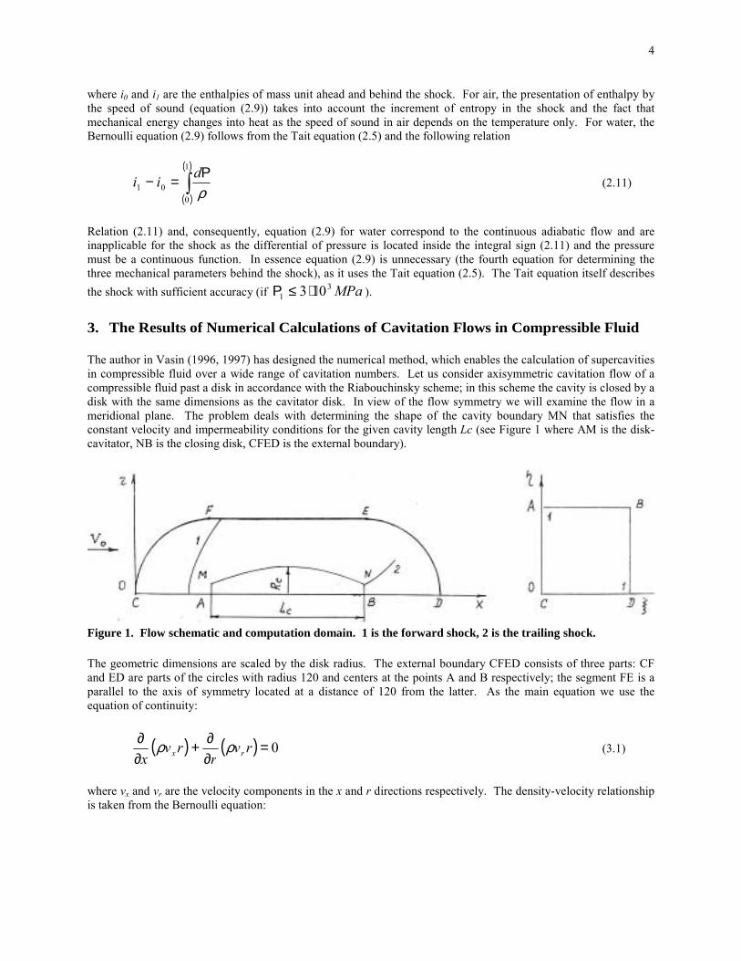
The author in Vasin (1996, 1997) has designed the numerical method, which enables the calculation of supercavities in compressible fluid over a wide range of cavitation numbers. Let us consider axisymmetric cavitation flow of a compressible fluid past a disk in accordance with the Riabouchinsky scheme; in this scheme the cavity is closed by a disk with the same dimensions as the cavitator disk. In view of the flow symmetry we will examine the flow in a meridional plane. The problem deals with determining the shape of the cavity boundary MN that satisfies the constant velocity and impermeability conditions for the given cavity length Lc (see Figure 1 where AM is the disk-cavitator, NB is the closing disk, CFED is the external boundary).

Figure 1. Flow schematic and computation domain. 1 is the forward shock, 2 is the trailing shock.

The geometric dimensions are scaled by the disk radius. The external boundary CFED consists of three parts: CF and ED are parts of the circles with radius 120 and centers at the points A and B respectively; the segment FE is a parallel to the axis of symmetry located at a distance of 120 from the latter. As the main equation we use the equation of continuity:

( ) ( ) 0=∂∂+

∂∂ rv

rrv

x rx ρρ (3.1)

where vx and vr are the velocity components in the x and r directions respectively. The density-velocity relationship is taken from the Bernoulli equation:

5

( ) ( )( )

15.7,1211

1/122

2

=

−−−+=

−

nvvMnn

rxρ (3.2)

In order to make the formulation of the boundary conditions at the cavity surface more convenient, it makes sense to map the computational domain in x, r coordinates onto a unit square in ξ, η coordinates. We consider the flow to be potential. In case of supersonic flow the shocks appear (see Figure 1; curve 1 is the forward shock formed upstream of the disk, curve 2 is the trailing shock emanating from the closing disk edge). The forward shock is the most intense and nearly normal in the vicinity of the symmetry axis. However, the shock�s appearance does not break the condition that the flow is potential. It is known (see Zamyshlyaev and Yakovlev (1967)) that when the pressure in water is less than 3⋅103 МPа a shock adiabat agrees with the static one expressed by the Tait equation (2.5). The analysis of equations (2.5) and (2.7) for the normal shock in water has shown that the pressure in the shock does not exceed 3⋅103 МPа if the Mach number is less than 2.2. Therefore, when М≤2.2 we can assume that the shock is isentropic and the flow is potential. In Vasin (1999) it is shown that we can determine the density from the Bernoulli equation (3.2) in the whole area of the supersonic flow if М≤2.2 (at the known flow velocity).

Thus, the main equations for the calculation of the supersonic cavitation flow are equations (3.1) and (3.2) as in the case of subsonic flow. We have applied the finite-difference method to solve these equations (see Vasin (1996, 1997)). In supersonic flow the boundary conditions on the external boundary differed from subsonic flow, and the artificial viscosity was applied in order for the difference scheme to be stable in the supersonic area.

The non-linear system of equations obtained as a result of the discretization was solved using the iteration method with approximate factorization. The iteration procedure turned out to be convergent; the discrepancy diminished, and the potential increment vanished as the number of the iteration cycles increased. However, in general, the obtained solution did not satisfy the impermeability condition on the cavity surface. In order to satisfy this condition the second iteration process was applied for varying the cavity shape. As a result of the numerical solution the obtained cavity shape satisfied both the constant velocity condition and the impermeability condition.

The numerical analysis was performed for the constant cavity length Lc=199.96 that corresponds with the cavitation number 0.02 for incompressible fluid (the cavitation number ( ) 000

2000 ,,,/2 VVc ρρσ ΡΡ−Ρ= where are

the pressure, density and velocity in free stream, Pc is the pressure within the cavity). The Mach number was within the range 0≤М≤1.4. As a result of the analysis for different Mach numbers the following parameters were defined: cavitation number, cavitation drag ratio, mid-section radius, aspect ratio, cavity shape, and the shock distance from a disk (for supersonic flow). The results of the numerical calculations satisfy the mass and momentum conservation laws. For subsonic and supersonic flows the cavity shape defined by the numerical calculations is close to an ellipsoid of revolution. It agrees with the author�s results obtained with the help of the slender body theory (see Vasin (1987, 1989)).

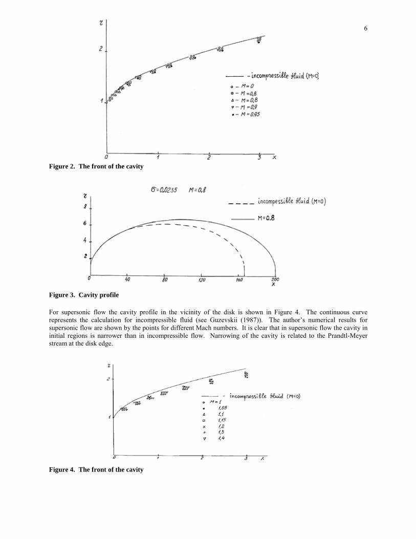
For subsonic flow the cavity shape in the vicinity of the disk is shown in Figure 2. The continuous curve represents Guzevskii (1987) calculation for incompressible fluid. The author�s numerical results for different Mach numbers are shown by the points. In Figure 3 we compare the cavity profiles in compressible and incompressible fluids for the same cavitation number σ=0.0235. The continuous curve corresponds with the cavity profile in a compressible fluid calculated by the numerical method for M=0.8; the stroke line curve corresponds to the cavity in an incompressible fluid calculated by the Logvinovich (1969) formula. Both of the cavity profiles are close to an ellipsoid of revolution. The dimensions of an ellipsoid for M=0.8 exceed the analogous dimensions for M=0 since the cavitation drag coefficient for M=0.8 exceeds the one for M=0.

6

Figure 2. The front of the cavity

Figure 3. Cavity profile

For supersonic flow the cavity profile in the vicinity of the disk is shown in Figure 4. The continuous curve represents the calculation for incompressible fluid (see Guzevskii (1987)). The author�s numerical results for supersonic flow are shown by the points for different Mach numbers. It is clear that in supersonic flow the cavity in initial regions is narrower than in incompressible flow. Narrowing of the cavity is related to the Prandtl-Meyer stream at the disk edge.

Figure 4. The front of the cavity

7

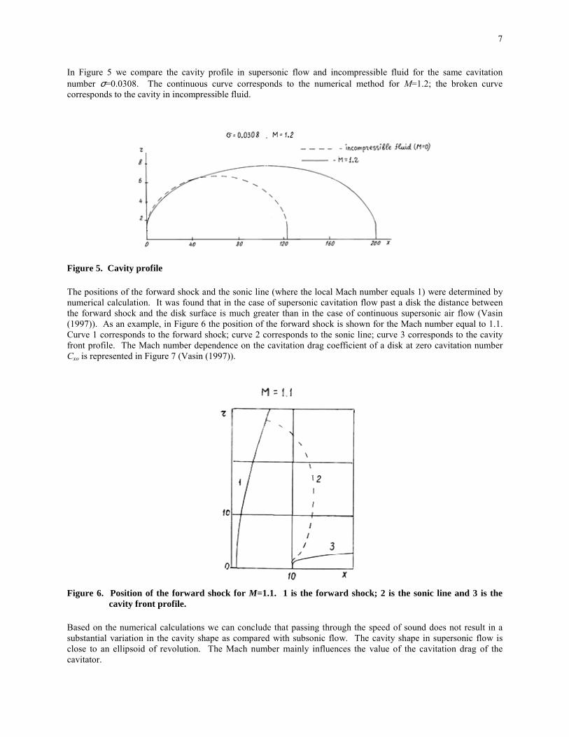
In Figure 5 we compare the cavity profile in supersonic flow and incompressible fluid for the same cavitation number σ=0.0308. The continuous curve corresponds to the numerical method for M=1.2; the broken curve corresponds to the cavity in incompressible fluid.

Figure 5. Cavity profile

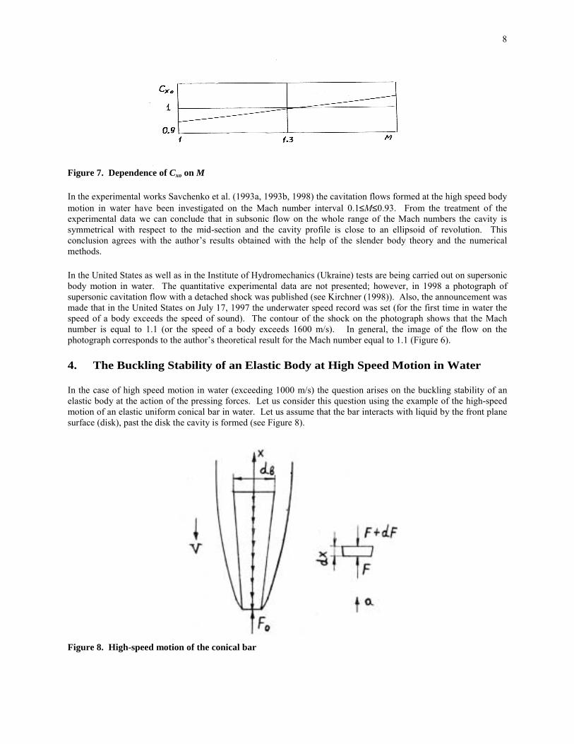
The positions of the forward shock and the sonic line (where the local Mach number equals 1) were determined by numerical calculation. It was found that in the case of supersonic cavitation flow past a disk the distance between the forward shock and the disk surface is much greater than in the case of continuous supersonic air flow (Vasin (1997)). As an example, in Figure 6 the position of the forward shock is shown for the Mach number equal to 1.1. Curve 1 corresponds to the forward shock; curve 2 corresponds to the sonic line; curve 3 corresponds to the cavity front profile. The Mach number dependence on the cavitation drag coefficient of a disk at zero cavitation number Схо is represented in Figure 7 (Vasin (1997)).

Figure 6. Position of the forward shock for M=1.1. 1 is the forward shock; 2 is the sonic line and 3 is the cavity front profile.

Based on the numerical calculations we can conclude that passing through the speed of sound does not result in a substantial variation in the cavity shape as compared with subsonic flow. The cavity shape in supersonic flow is close to an ellipsoid of revolution. The Mach number mainly influences the value of the cavitation drag of the cavitator.

8

Figure 7. Dependence of Cxo on M

In the experimental works Savchenko et al. (1993a, 1993b, 1998) the cavitation flows formed at the high speed body motion in water have been investigated on the Mach number interval 0.1≤М≤0.93. From the treatment of the experimental data we can conclude that in subsonic flow on the whole range of the Mach numbers the cavity is symmetrical with respect to the mid-section and the cavity profile is close to an ellipsoid of revolution. This conclusion agrees with the author�s results obtained with the help of the slender body theory and the numerical methods.

In the United States as well as in the Institute of Hydromechanics (Ukraine) tests are being carried out on supersonic body motion in water. The quantitative experimental data are not presented; however, in 1998 a photograph of supersonic cavitation flow with a detached shock was published (see Kirchner (1998)). Also, the announcement was made that in the United States on July 17, 1997 the underwater speed record was set (for the first time in water the speed of a body exceeds the speed of sound). The contour of the shock on the photograph shows that the Mach number is equal to 1.1 (or the speed of a body exceeds 1600 m/s). In general, the image of the flow on the photograph corresponds to the author�s theoretical result for the Mach number equal to 1.1 (Figure 6).

4. The Buckling Stability of an Elastic Body at High Speed Motion in Water

In the case of high speed motion in water (exceeding 1000 m/s) the question arises on the buckling stability of an elastic body at the action of the pressing forces. Let us consider this question using the example of the high-speed motion of an elastic uniform conical bar in water. Let us assume that the bar interacts with liquid by the front plane surface (disk), past the disk the cavity is formed (see Figure 8).

Figure 8. High-speed motion of the conical bar

9

The drag force F0 acts on the bar. The bar is in the state of equilibrium if in accordance with d�Alembert�s principle the distributed load of inertial forces q(x) acts on it. Let us determine the distributed load from the condition of equilibrium of bar element with the length equal to dx (Figure 8). The resultant force dF that acts on the element equals the inertial force:

admdF ⋅−= (4.1)

where dm is the mass of the element, а is the longitudinal acceleration from the action of the drag force ( )mFaF /00 = , m is the mass of the bar. The mass of the element is written in the form

( )dxxRdm m2πρ=

where ρm is the density of bar material, R(x) is the radius of bar cross-section corresponding to х coordinate. The distributed load ( )dxdFq /= has the following representation:

( ) ( )m

xRFxq m

20 πρ

−= (4.2)

The pressing force F(x) on the bar section that corresponds to x coordinate is written as follows:

( ) ( )dxxRm

FFxF

xm ∫−=

0

200

πρ (4.3)

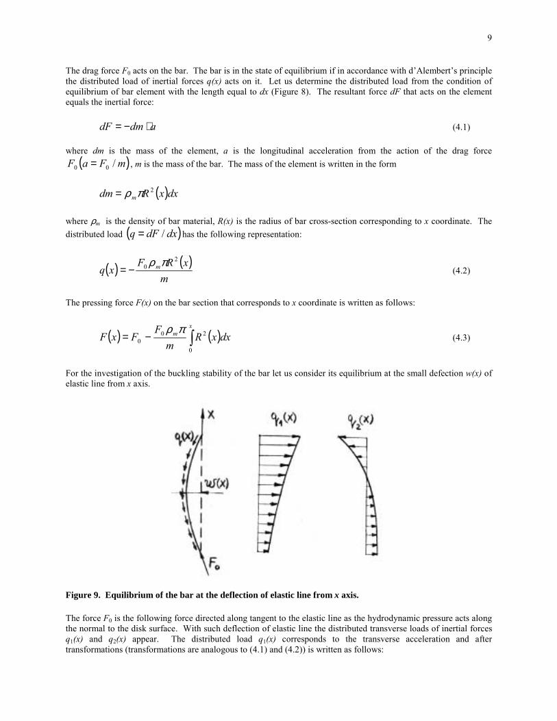
For the investigation of the buckling stability of the bar let us consider its equilibrium at the small defection w(х) of elastic line from x axis.

Figure 9. Equilibrium of the bar at the deflection of elastic line from x axis.

The force F0 is the following force directed along tangent to the elastic line as the hydrodynamic pressure acts along the normal to the disk surface. With such deflection of elastic line the distributed transverse loads of inertial forces q1(x) and q2(x) appear. The distributed load q1(x) corresponds to the transverse acceleration and after transformations (transformations are analogous to (4.1) and (4.2)) is written as follows:

10

( ) ( ) ( )m

xRowFxq m

20

1πρ′

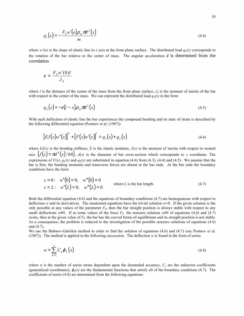
−= (4.4)

where w′(о) is the slope of elastic line to х axis at the front plane surface. The distributed load q2(x) corresponds to the rotation of the bar relative to the center of mass. The angular acceleration ε is determined from the correlation

0

0 )0(J

lwF ′=ε

where l is the distance of the center of the mass from the front plane surface, J0 is the moment of inertia of the bar with respect to the center of the mass. We can represent the distributed load q2(x) in the form

( ) ( ) ( )xRxlxq m2

2 πρε −−= (4.5)

With such deflection of elastic line the bar experiences the compound bending and its state of strain is described by the following differential equation (Postnov et al. (1987))

( ) ( )[ ] ( ) ( )[ ] ( ) ( )xqxqxwxFxwxEJ 21 +=′′+″′′ (4.6)

where EJ(x) is the bending stiffness, Е is the elastic modulus, J(x) is the moment of inertia with respect to neutral axis ( ) ( )( )64/4 xdxJ π= , d(x) is the diameter of bar cross-section which corresponds to x coordinate. The expressions of F(x), q1(x) and q2(x) are substituted in equation (4.6) from (4.3), (4.4) and (4.5). We assume that the bar is free; the bending moments and transverse forces are absent at the bar ends. At the bar ends the boundary conditions have the form

( ) ( )( ) ( ) 0,0:

00,00:0=′′′=′′=

=′′′=′′=LwLwLx

wwx where L is the bar length. (4.7)

Both the differential equation (4.6) and the equations of boundary conditions (4.7) are homogeneous with respect to deflection w and its derivatives. The mentioned equations have the trivial solution w=0. If the given solution is the only possible at any values of the parameter F0, then the bar straight position is always stable with respect to any small deflections w≠0. If at some values of the force F0 the nonzero solution w≠0 of equations (4.6) and (4.7) exists, then at the given value of F0 the bar has the curved forms of equilibrium and its straight position is not stable. As a consequence, the problem is reduced to the investigation of the possible nonzero solutions of equations (4.6) and (4.7). We use the Bubnov-Galerkin method in order to find the solution of equations (4.6) and (4.7) (see Postnov et al. (1987)). The method is applied in the following succession. The deflection w is found in the form of series

( )xCw k

n

kkϕ∑

=

=1

(4.8)

where n is the number of series terms dependent upon the demanded accuracy, Ск are the unknown coefficients (generalized coordinates), ϕк(х) are the fundamental functions that satisfy all of the boundary conditions (4.7). The coefficients of series (4.8) are determined from the following equations:

11

( ) ( ) ( ) ( ) ( )[ ] ( ) ;0

210

dxxxqxqdxxwFwEJ i

L

i

L

ϕϕ ∫∫ +=

′′+″′′ i=1,2,�, n (4.9)

Equations (4.9) are obtained after multiplying the differential equation of compound bending (4.6) by functions ϕi(х) and integrating the bar length. We can write as many of these equations as expression (4.8) contains the series terms. Let us substitute expression (4.8) in equation (4.9). After interchanging the order of integration and summing up we obtain

( ) niBCFA ik

n

kkiki ,...,2,1,

1==+∑

=

(4.10)

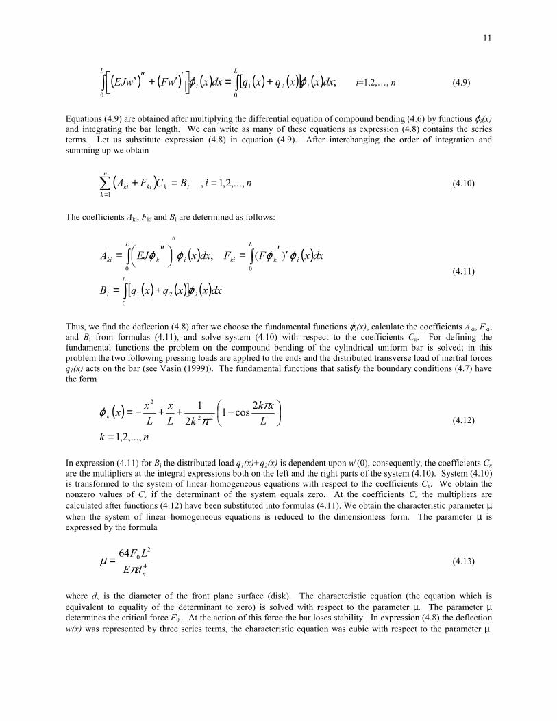
The coefficients Aki, Fki and Bi are determined as follows:

( ) ( )

( ) ( )[ ] ( )dxxxqxqB

dxxFFdxxEJA

i

L

i

i

L

kkii

L

kki

ϕ

ϕϕϕϕ

∫

∫∫

+=

′′=″

″=

021

00

)(, (4.11)

Thus, we find the deflection (4.8) after we choose the fundamental functions ϕi(x), calculate the coefficients Aki, Fki, and Bi from formulas (4.11), and solve system (4.10) with respect to the coefficients Ск. For defining the fundamental functions the problem on the compound bending of the cylindrical uniform bar is solved; in this problem the two following pressing loads are applied to the ends and the distributed transverse load of inertial forces q1(x) acts on the bar (see Vasin (1999)). The fundamental functions that satisfy the boundary conditions (4.7) have the form

( )

nkL

xkkL

xLxxk

,...,2,1

2cos12

122

2

=

−++−= π

πϕ

(4.12)

In expression (4.11) for Bi the distributed load q1(x)+q2(x) is dependent upon w′(0), consequently, the coefficients Ск are the multipliers at the integral expressions both on the left and the right parts of the system (4.10). System (4.10) is transformed to the system of linear homogeneous equations with respect to the coefficients Ск. We obtain the nonzero values of Ск if the determinant of the system equals zero. At the coefficients Ск the multipliers are calculated after functions (4.12) have been substituted into formulas (4.11). We obtain the characteristic parameter µ when the system of linear homogeneous equations is reduced to the dimensionless form. The parameter µ is expressed by the formula

4

2064

ndELF

πµ = (4.13)

where dn is the diameter of the front plane surface (disk). The characteristic equation (the equation which is equivalent to equality of the determinant to zero) is solved with respect to the parameter µ. The parameter µ determines the critical force F0 . At the action of this force the bar loses stability. In expression (4.8) the deflection w(х) was represented by three series terms, the characteristic equation was cubic with respect to the parameter µ.

12

Three values of µ were obtained from the solution of the cubic equation. The minimum value of the critical force corresponds to the minimum value µ. Let us determine the value of the bar aspect ratio λ, ( )ndL /=λ that corresponds to the stability loss for the given motion speed V. The force F0 is written in the form

8

22

0nx dVC

Fπρ

= (4.14)

where Ск is the drag coefficient. The numerical calculations have shown (see Vasin (1996, 1997)) that on the transonic velocity range the disk coefficient Ск is approximately equal to 1 and it increases insignificantly as the Mach number increases. Let us take the value of Ск equal to 1. After substituting (4.14) in (4.13) we obtain the expression for the bar aspect ratio:

28 VCE

x ρµλ = (4.15)

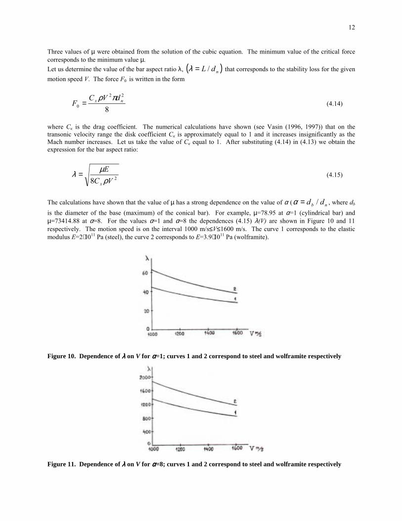
The calculations have shown that the value of µ has a strong dependence on the value of α ( nb dd /=α , where db is the diameter of the base (maximum) of the conical bar). For example, µ=78.95 at α=1 (cylindrical bar) and µ=73414.88 at α=8. For the values α=1 and α=8 the dependences (4.15) λ(V) are shown in Figure 10 and 11 respectively. The motion speed is on the interval 1000 m/s≤V≤1600 m/s. The curve 1 corresponds to the elastic modulus Е=2⋅1011 Pa (steel), the curve 2 corresponds to Е=3.9⋅1011 Pa (wolframite).

Figure 10. Dependence of λλλλ on V for αααα=1; curves 1 and 2 correspond to steel and wolframite respectively

Figure 11. Dependence of λλλλ on V for αααα=8; curves 1 and 2 correspond to steel and wolframite respectively

13

Conclusions

The basic correlations for shock in water have been considered. It is shown that the application of the equations of compressible gas supersonic flow for the equations that describe shocks in water leads to an erroneous result.

The supersonic cavitation flow in water has certain peculiarities. The cavity has remarkable characteristics; it promotes not only the motion in water with small drag but also screens the body from shocks. On the cavity surface the constant velocity and the constant pressure conditions are satisfied, consequently the shocks are absent. The bow shock forms before the cavitator or on its apex (in case of thin cones), in the domain of cavity closure the trailing shock forms. For this scheme of flow the sharp change of the flow parameters does not occur on the transonic velocity range. As distinct from water, in air on the transonic velocity range the shocks form on the body surface and aerodynamic characteristics of body change considerably. In water, on the transonic velocity range the parameters of the cavitation flow change smoothly as the Mach number increases. Passing through the speed of sound does not result in a substantial variation in the cavity shape as compared to subsonic flow. In spite of the small asymmetry of the shape about the mid-section the cavity shape in supersonic flow is close to an ellipsoid of revolution as it was before.

Water is a rather slightly compressible fluid as compared with air. In water many physical effects connected with compressibility essentially differ from those in air. We can assume that the normal shock in water is isentropic and the flows are potential at the Mach numbers on the interval 1<M≤2.2. At the same Mach numbers the ratio of densities ρ1/ρ0 on the shock front in water is far less than that in air. As a result the distance between the bow shock and the cavitator surface in water is much greater than in case of continuous supersonic air flow. The flow turning angle for the Prandtl-Meyer stream in water is far less than that in air at the same Mach numbers. All the factors mentioned above (the small losses of mechanical energy in the shocks, the considerable distance between the bow shock and the cavitator surface, the small deflection of flow in the stream about the cavitator edge) enable the cavity expansion. In supersonic flow at the Mach numbers on the interval 1≤M≤1.4 we do not observe the considerable narrowing and change of the cavity shape as compared with subsonic flow. The cavity expands in accordance with the law of conservation of energy in a fluid.

The buckling stability of elastic body moving at a high speed in water has been investigated. As an example the elastic uniform conical bar is considered. The values of aspect ratio of the bar that correspond to stability loss are defined for the different values of motion speed.

References

Al�ev G. A. (1984). Supersonic Water Separation Flow Past a Circular Cone of Finite Length. in Dynamics of Continuum with Non-Steady Boundaries. Chuvash. Univ. Press, Cheboksary, 3-7 (in Russian) Cole R. H. (1948). Underwater Explosions. University Press, Princeton. Guzevskii L. G. (1987). Plane and Axisymmetric Problems of Hydrodynamics with Free Surface. Dissertation for a doctor�s degree, Institute of Thermal Physics, Siberian Branch of the USSR Academy of Sciences, Novosibirsk, 300 (in Russian). Kirchner I. N. (1998). Supercavitating Projectile Experiments at Supersonic Speeds. Abstract in High-Speed Body Motion in Water, AGARD-R-827. Reference 35. Korobeinikov V. P. and Cristoforov B. D. (1976). Underwater Explosion. Itogi nauki i technili, Hydromechanics, VINITI, Moscow, 9, 54-119 (in Russian). Logvinovich G. V. (1969). Hydrodynamics of Flows with Free Boundaries. Naukova Dumka, Kiev, 215 (in Russian) Nishiyama T. and Khan O. F. (1981). Compressibility Effects on Cavitation in High Speed Liquid Flow (Second Report � Transonic and Supersonic Liquid Flows). Bull. JSME, v. 24, 190, 655-661. Postnov V. A., Rostovtsev D. M., Suslov V. P. and Kochanov Yu. P. (1987). Marine Engineering and the Theory of Elasticity. v.2, Sudostroenie, Leningrad, 412 (in Russian).

14

Savchenko Yu. N., Semenenko V. N. and Serebryakov V. V. (1993a). Experimental Check of Asymptotic Formulas for Axisymmetric Cavities at σ→0. In Problems of High-Speed Hydrodynamics. Chuvash. University Press, Cheboksary, 117-122 (in Russian). Savchenko Yu. N., Semenenko V. N. and Serebryakov V. V. (1993b). Experimental Investigation of Developed Cavitating Flows at Subsonic Flow Velocities. Dokl. Akad. Nauk Ukraine, 2, 64-69 (in Russian). Savchenko Yu. N. (1998). Investigation of High-Speed Supercavitating Underwater Motion of Bodies. In High-Speed Body Motion in Water. AGARD-R-827, Reference 20. Stanyukovich K. P. (1971). Unsteady Motion of a Continuum. Nauka, Moscow, 854 (in Russian). Vasin A. D. (1987). Thin Axisymmetric Cavities in Subsonic Compressible Flow. Izv. Akad. Nauk SSSR, Mekh. Zhidk. Gaza, 5, 174-177 (reprinted in the USA). Vasin A. D. (1989). Thin Axisymmetric Cavities in Supersonic Flow. Izv. Akad. Nauk SSSR, Mekh. Zhidk. Gaza, 1, 179-181 (reprinted in the USA). Vasin A. D. (1996). Calculation of Axisymmetric Cavities Downstream of a Disk in Subsonic Compressible Fluid Flow. Izv. Rus. Akad. Nauk, Mekh. Zhidk. Gaza, 2, 94-103 (reprinted in the USA). Vasin A. D. (1997). Calculation of Axisymmetric Cavities Downstream of a Disk in Supersonic Flow. Izv. Rus. Akad. Nauk, Mekh. Zhidk. Gaza, 4, 54-62 (reprinted in the USA). Vasin A. D. (1999). Problems of Hydrodynamics and Hydroelasticity at High Speed Body Motion in Water. Dissertation for a doctor�s degree, TsAGI, Moscow, 282 (in Russian). Vasin A. D. (2000). High-Speed Body Motion in Compressible Fluid. In Proceedings of the Scientific Meeting on High-Speed Hydrodynamics and Supercavitation. Laboratoire des Ecoulements Geophysiques et Industriels, Grenoble, France. Zamyshlyaev B. V. and Yakovlev Yu. S. (1967). Dynamic Loads in Underwater Explosions. Sudostroenie, Leningrad. 387 (in Russian).