SOME OBSERVATIONS ON THE ECOLOGY AND …

SOME OBSERVATIONS ON THE ECOLOGY AND BIOCHEMICALASPECTS OF THE SEAWEEDS OF KERALA COAST

THESIS SUBMITTED BY

SAJI SUSAN MATHEW, M. SC.

TO THE COCHIN UNIVERSITY OF SCIENCE AND TECHNOLOGYIN PARTIAL FULFILMENT OF THE REQUIREMENTS FOR

AWARD OF THE DEGREE OFDOCTOR OF PHILOSOPHY

ICAR

CENTRE OF ADVANCED STUDIES IN MARICULTURECENTRAL MARINE FISHERIES RESEARCH INSTITUTE

KOCHI - 682 031 INDIA

|99|

DECLARATION

I hereby declare that the thesis entitled Some observations on the

ecology and biochemical aspects of the seaweeds of Kerala coast has not

previously formed the basis of the award of any degree, diploma, associate

ship, fellowship or other similar title or recognition.

Kochi - 31 /(jc//ob/zwA AJanuary, 1991 " JI SUSAN MATHEW)

CERTIFICATE

This is to certify that this thesis is an authentic record of the work

carried out by Miss. Saji Susan Mathew, under my supervision at Central Marine

Fisheries Research Institute and no part thereof has been presented before for

any other degree in any University.

/4/2 )3‘;Dr: V.S. K. CHENNUBHOTLA

Principal ScientistCentral Marine FisheriesK0Chi ‘ 31 Research Institute

Kochi — 682 031"‘Im January’ 1991' (Supervising Teacher)

ACKNOWLEDGEMENTS

It is with great pleasure that I place on record, my indebtedness

and deepest sense of gratitude to my revered teacher Dr.V.S. Krishnamurthy

Chennubhotla, Principal Scientist, Minicoy Research Centre of Central Marine

Fisheries Research Institute, for his able guidance, thorough supervision,

valuable suggestions, constant help and encouragement throughout the course

of this work. I consider it my singular good fortune for having worked

as a research scholar under him, and I feel that I was greatly benefitted

for being so well initiated into the field of marine algal research by him.

I will be failing in my duty if on this occasion, I do not make a

special mention of the multifarious help and advice extended to me by

Dr.C.V. Kurien, Professor Emeritus, School of Marine Sciences, Cochin

University of Science and Technology, Kochi.

I recall with gratitude, Dr. Desikachary the eminent botanist and

authority on algae for the advice, encouragement and affection shown tome.

My thanks are due to Dr. V. Krishnamurthy, Professor, Department

of Botany, Centre for Advanced Studies, Madras for the confirmation of

the algal identifications and for the healthy discussions I had with him.

I express my gratitude to Mr. T.N. Rajan, Geologist, Geological

Survey of India, Kochi, for sparing his valuable time for discussions with

me.

My sincere thanks are also due to Mr. M. Srinath, Scientist, Central

Marine Fisheries Research Institute, Kochi for helping me with the statistical

analysis of my data.

In this context, I like to express my gratitude to Mr.A. Nandakumar

for the immense and untiring help he rendered throughout the period of

my work.

I thank Dr. P.S.B.R. James, Director, Central Marine Fisheries

Research Institute, Kochi, for the facilities provided for doing this research

work.

Above all, I thank Indian Council of Agricultural Research for awarding

me with the Senior Research Fellowship during the tenure of which I did

this work.

SOME OBSERVATIONS ON THE ECOLOGY AND BIOCHEMICAL

ASPECTS OF THE SEAWEEDS OF KERALA COAST

CONTENTS

PREFACE

1.1 Seaweeds as food

1.2 Seaweeds in industry

1.2.1 Agar-agar

1.2.2 Algin

1.2.3 Carrageenan

1.3 Seaweeds in medicine

1.4 Seaweeds as fodder

1.5 Seaweeds as manure

1.6 Seaweeds as a source of vitamins

1.7 Seaweeds as a source of energy

1.8 Seaweed ecosystem

INTRODUCTION

2.1 Places of algal interest in India

2.2 Objectives of the present study

MATERIALS AND METHODS

3.1 Ecological features of Kerala coast

3.2 Shoreline of Kerala

Page No.

vi

vi

vii

vii

3.3

3.4

3.5

3.6

3.7

3.7.1

3.7.2

3.7.3

3.7.4

3.7.5

3.8

3.8.1

3.8.2

3.8.3

Geology of Kerala coast

Tides and storm tides of Kerala

Waves of Kerala coast

Metereological features of Kerala

Description of the study area

Elathur

Thikkotti

Varkala

Mullur

Saudi

Methods of study

Determination of seaweed density

Hydrological studies

Biochemical studies

ECOLOGICAL OBSERVATIONS

4.1

4.2

4.2.1

LIST OF SEAWEEDS RECORDED FROM KERALACOAS'I‘ DURING THE PRESENT STUDY

ECONOMICALLY IMPORTANT SEAWEEDS OFKERALA COAST

Commercially important seaweeds ofKerala coast

4. 2.2 Edible seaweeds of Kerala coast

Page No.

10

10

11

12

12

12

13

13

15

15

20

20

21

4.3

4.3.1

4.3.2

4.3.3

4.4

4.5

4.5.1

4.5.2

4.5.3

4.5.4

4.5.5

4.6

4.6.1

4.6.2

4.6.3

4.7

4.7.1

DISTRIBUTION OF SEAWEEDS INDIFFERENT ZONES OF KERALACOAST

Seaweeds from North zone of Kerala coast

Seaweeds from South zone of Kerala coast

Seaweeds from Central zone of Kerala coast

ZONATION PATTERN OF SEAWEEDS ALONGKERALA COAST

DENSITY OF SEAWEEDS IN DIFFERENTSTATIONS ALONG KERALA COAST

Density of seaweeds at Mullur

Densi‘y of seaweeds at Varkala

Density of seaweeds at Elathur

Density of seaweeds at Thikkotti

Density of seaweeds at Saudi

FREQUENCY OF OCCURRENCE OF SEAWEEDSALONG KERALA COAST

Seaweed species showing very high frequency ofoccurrence along Kerala coast

Seaweed species showing high frequency ofoccurrence along Kerala coast

Seaweed species showing low frequency ofoccurrence along Kerala coast

STANDING CROP OF SEAWEEDS ALONG KERALACOAST

Standing crop of economically importantseaweeds along Kerala coast

Page No.

22

22

26

29

32

34

35

41

46

50

55

60

61

62

63

65

65

4.8

4.8.1

4.8.2

4.8.3

4.8.4

4.9

ENVIRONMENTAL FEATURES OF KERALA COAST

Environmental data recorded at various stations

Seasonal variation in environmental datarecorded at the various stations

Comparison of environmental data from differentstations

Correlation between environmental factors observedat the various stations

CORRELATION BETWEEN ENVIRONMENTALFACTORS AND THE DENSITY OF SEAWEEDS

BIOCHEMICAL OBSERVATIONS

5.1

5.1.1

5.1.2

5.1.3

5.1.4

5.1.5

5.2

5.2.1

BIOCHEMICAL COMPOSITION OF SEAWEEDS FROMVARIOUS STATIONS ALONG KERALA COAST

Biochemical composition of some seaweeds fromMullur

Biochemical composition of some seaweeds fromVarkala

Biochemical composition of some seaweeds fromElathur

Biochemical composition of some seaweeds fromThikkotti

Biochemical composition of some seaweeds fromSaudi

SEASONAL VARIATION IN BIOCHEMICALCOMPOSITION OF SOME SELECTED SEAWEEDSFROM VARIOUS STATIONS ALONG KERALACOAST

Seasonal variation in biochemical composition ofsome selected seaweeds from Mullur

Page No.

69

69

74

79

85

87

91

91

91

106

114

123

131

143

143

5.2.2 Seasonal variation in biochemical compositionof some selected seaweeds from Varkala

5.2.3 Seasonal variation in biochemical compositionof sonic selected seavveeds froni Elathur

5.2.4 Seasonal variation in biochemical compositionof two selected seaweeds from Thikkotti

5.2.5 Seasonal variation in biochemical compositionof two selected seaweeds from Saudi

5.3 PLACE-WISE VARIATION IN BIOCHEMICALCOMPOSHWON

54 PARAMETERSSHOWHK3CORRELAHONWITH BIOCHEMICAL CONSTITUENTS OFSEAWEEDS

DISCUSSION

&1 ECOLOGY OFSEAWEEDS

6.1.1 Environrnental factors controning speciescomposition, distribution and density ofseaweeds

6.1.2 Seasonal changes in species composition,distribution and density of seaweeds

6.1.3 Standing crop of seaweeds along Kerala coast

6.1.4 Zonation of seaweeds along Kerala coast

6.2 BIOCHEMICAL COMPOSITION OF SEAWEEDS

SUMMARY

REFERENCES

Page No.

150

153

158

162

165

172

173

173

176

187

195

198

201

208

213

1. PREFACE

While the common man is familiar with land plants, the world of

marine plants is a hidden world for him. Today, envisaging the continued

growth of the world's population, man is increasingly turning his attention

to the plant life of the oceans as a major source of food and industrial

raw materials.

Marine plants primarily fall under two evolutionary divergent groups,

the primitive plants - algae — and the most advanced plants - angiosperms.

Among the angiosperms only a small group - seagrasses - is represented

in the sea. About 90% of the marine plants, belong to one group of algae

or the other. Thus vegetation-wise the sea remains to this day, a province

of algae.

Under the term algae, we group a large number of simple plants

which originated at different levels on the evolutionary scale. Among

the marine algae, the macroscopic algae — seaweeds — form a very important

living renewable resource of the oceans. They are available in the coastal

waters, wherever there is a substratum on which they can grow and flourish.

Based on their pigmentation they are grouped into three major divisions

Chlorophyta (green algae), Phieophyta (brown algae) and Rhodophyta (red

algae).

Economically seaweeds have proved themselves to be a very significant

group.

1.1 Seaweeds as food

Seaweeds have been harvested since many centuries in the South

East Asian countries where they form staple human food. Many of the

seaweeds are eaten raw or processed, in many parts of the world.

The nutritive value of the seaweeds lie in the fact that they are

very rich in proteins, carbohydrates and lipids. They also contain more

than 60 trace elements, in concentrations, higher than that in terrestrial

plants. The algal proteins have many essential amino acids including iodine

containing ones. The seaweed Porphyra vietnamensis is reported to contain

16-30% protein on dry weight basis, and this amount is higher than that

of cereals, eggs and fish (Visweswara Rao, 1964). Other seaweeds like

Ulva fasciata, E. lactuca, E. rigida, Centroceras clavulatum etc., are also

rich in protein. In Japan about 21 varieties of seaweeds are being used

as sea-vegetables in everyday cookery. According to Fujiwara e_tfl(1983) Japanese consume seaweeds as much as 1.6 kg (dry) per capita annual.

The thin delicate red seaweed Porphyra is processed and used as a culinary

dish known as 'Laver' in Britain and 'Nori' in Japan (Chapman and Chapman

1980). Apart from this, the Japanese use 'Kombu' a preparation out of

Laminaria and 'Wakame' a preparation out of Undaria in their daily diet.

It is reported that 100 gm of algae per day provide all that a human

being needs in respect of sodium, potassium and magnesium (Chapman and

Chapman, 1980).

In India, except for the use of Gracilaria edulis for making gruel

in the coastal areas of Tamil Nadu, seaweeds are not being directly used

iii

as food (Anon, 1987). Seaweeds as food has a great potential in India

where 60% of the population are vegetarians.

1.2 Seaweeds in industry

Seaweeds are the only source of phyco—co1loids, viz., agar-agar,

algin and carrageenan. These phytochemicals are extensively used in various

industries like food, confectionary, textile, cosmetics, paper, pharmaceutical,

dairy, paint etc., mainly as gelling, stabilising and thickening agents.

1.2 .1 Agar-agar

It is a_gelatinous colloidal carbohydrate present in the cell walls

of some red algae. It is a mixture of two polysaccharides, agarose and

agaropectin. This substance has the property of forming a gel on cooling.

The best known use of agar is as a solidifying agent in bacteriological

culture media. Apart from this, it finds use in various industries, mentioned

before. The market value of I.P. grade and food grade agar in India is

Rs.500/- and Rs.200/- respectively (Anon, 1990).

Agar yielding seaweeds are called agarophytes and some important

agarophytes of Indian waters are Gelidiella acerosa, Gracilaria edulis,

G. corticata, Q. crassa, Q. foliifera and Q. verrucosa.

1.2.2 Algin

Algin is a polysaccharide occurring in the cell walls of brown algae.

It consists of D—mannuronic acid and 2-guluronic acid in various proportions.

The sodium, potassium and magnesium salts of alginic acid are soluble

in water and they give a viscous liquid without gel formation. Algin also

has a variety of industrial uses. The market rate of sodium alginate varies

from Rs.90/- to Rs.120/- depending on its quality (Anon, 1990).

Algin yielding seaweeds are called alginophytes and important among

them in India being species of Sargassum and Turbinaria.

1.2.3 Carrageenan

Certain red algae produce gel-like extracts called agaroids. They

differ in their properties and chemical nature from agar. Carrageenan

comes under this group. Organic sulphate content in these compounds

is very high. Pure solutions of agaroids are viscous and do not form gel

when cooled. But inorganic and organic solutes can alter the properties

of agaroids and improve their gelling power.

Important carrageenan yielding seaweeds of India are Gigartina

acicularis, Hypnea musciformis, species of Acanthophora, Laurencia, Sarconema

Spyridea and Chondria. Apart from these, seaweeds yield phycocolloids

of lesser importance but very valuable in specific uses like mannitlol,

laminarin, fucoidin etc.

In India, seaweeds are being commercially exploited from Tamil

Nadu and Gujarat coasts since 1962. At present there are about 21 agar

and 25 algin manufacturing industries in our country (Anon, 1987).

1.3 Seaweeds in medicine

Various red algae like Corallina officinalis, Q. rubens and Alsidium

helminthocorton are being employed as vermifuge from ancient times. Dulse

is being used in the treatment of goitre (Umamaheswara Rao, 1970). Range

of iodine in Indian seaweeds is 0.02 - 0. 024% on dry weight basis (Thivy,

1958). Antibiotic substance extracted from Enteromorpha affected complete

inhibition of ‘tubercle bacilli’ in cultures (Sreenivasa Rao gt.a_l., 1979).

Hundred percent antifertility activity was observed in three species of

algae namely Padina tetrastromatica, Gelidiella acerosa and Acanthophora

spicifera (Naqvi et a1., 1981). Extracts of Chondrus crispus and Gelidium

cartilagineum have been found to be active against influenza B and mumps

virus (Garber et a1., 1958). Analgesic, mild anesthetic, anticoagulant,

anti-inflammatory, antilipemic and antitumour activities are also reported

from marine macroalgae. Apart from this, agar and algin are being exten

sively used in pharmaceutical preparations. Agar is used in the manufacture

of dental impression moulds. Alginates when injected into the lung cavities

of tuberculosis patients, stop internal bleeding (Thivy, 1958).

1.4 Seaweeds as fodder

Seaweeds are rich sources of proteins, lipids, carbohydrates, trace

elements, vitamins etc. Hence it has been tried as animal feed in many

countries, the world over. Some experiments have shown that seaweed

meal improves the fertility and birth rate of animals. Stephenson (1974)

suggested that this may be due to the presence of antisterility Vit-E

(tocopherol). Seaweed meal has been found to improve the iodine content

of eggs (Thivy, 1958) and colour of egg yolk. Seaweed feeds have been

used extensively in the farming of milkfish successfully (Thivy, 1958).

Enteromorpha clathrata feed used in prawn culture fields has been found

to improve their growth and survival rates (Krishnamurthy, e_t gl., 1982).

vi

In conclusion it may be said that seaweed meal upto 10% in the basic

daily ration has beneficial effects on animals.

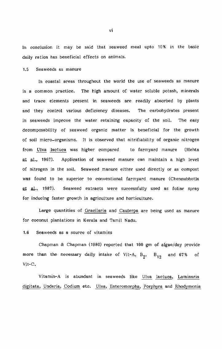
1.5 Seaweeds as manure

In coastal areas throughout the world the use of seaweeds as manure

is a common practice. The high amount of water soluble potash, minerals

and trace elements present in seaweeds are readily absorbed by plants

and they control various deficiency diseases. The carbohydrates present

in seaweeds improve the water retaining capacity of the soil. The easy

decomposability of seaweed organic matter is beneficial for the growth

of soil micro.-organisms. It is observed that nitrifiability of organic nitrogen

from fly; lactuca was higher compared to farmyard manure (Mehta

at al., 1967). Application of seaweed manure can maintain a high level

of nitrogen in the soil. Seaweed manure either used directly or as compost

was found to be superior to conventional farmyard manure (Chennubhotla

e_t a1., 1987). Seaweed extracts were successfully used as foliar spray

for inducing faster growth in agriculture and horticulture.

Large quantities of Gracilaria and Caulerpa are being used as manure

for coconut plantations in Kerala and Tamil Nadu.

1.6 Seaweeds as a source of vitamins

Chapman dc Chapman (1980) reported that 100 gm of algae/day provide

more than the necessary daily intake of Vit-A, B B and 67% of2’ 12Vit-C.

Vitamin-A is abundant in seaweeds like Ulva lactuca, Laminaria

flitata, Undaria, Codium etc. Ulva, Enteromorpha, Porphyra and Rhodymenia

vii

are rich in Vitamin B1. Vitamin C is abundant in E, Enteromorpha,Porphyra etc. Weight for weight, dulse contains half as much Vitamin C as in oranges. Niacin is present in marine algae in quantities ranging

from 1-68 /ugg—1 dry weight. Other vitamins detected in marine algae

include pantothenic acid, folic acid and Vitamins D dc E.

1.7 Seaweeds as a source of energy

Two thirds of the total solar energy which reaches the surface of

our planet falls on water. The energy is captured by algae - the abundant

photosynthetic organisms which grow in water. Thus seaweeds can potentially

be used as biomass for energy production (Bird and Benson, 1987). Seaweeds

contribute to 50% of the total marine primary productivity on an year

round basis.

1.8 Seaweed ecosystem

In addition to their commercial importance, macroalgae together

with a number of marine and estuarine angiosperms, play an important

role in many marine ecosystems. They provide habitation and spawning

sites for commercially important marine animals and make a significant

contribution to the food of man. Their contribution can be viewed more

importantly as a source of organics leading to detrital food chains of

demersal fish species. Devastation of seaweed beds through grazing by

predators or other means have been found to cause serious ecological

imbalances which in turn has significant fisheries interactions.

Many marine algae have the capacity to selectively concentrate

different trace elements and thus are useful in radio—active research as

viii

biological monitors. This will be of particular use in the radioactive waste

water treatment of oceans.

Seaweeds, thus are very important, not only for their economic

uses, but also for their biological role in marine environments. Therefore,

there seems to be a great potential in investigating into the basic biological

problems of seaweeds, especially their ecology and biochemical composition.

2. INTRODUCTION

Despite numerous investigations on the ecology of marine plants,

the subject has not advanced as much as the ecology of terrestrial plants,

because, unlike the study of land vegetation, field experiments are more

difficult in marine environment.

Considering the importance of marine algae, especially seaweeds

as food and raw material for industrial products, it is surprising that no

attempt has been made so far to survey its resources until the beginning

of the present century. This may be attributed to the unfamiliarity on

the importance and potentials of seaweed resources, or to the fact that

there seemed to be such an abundance of seaweeds in the past, that it

did not seem worthwhile attempting to estimate the quantities available.

However, due to the continued growth of the world's population resulting

in increasing pressure for food and energy, seaweeds which form an annually

renewable resource is becoming increasingly important.

2.1 Places of algal interest in India

India, has a coastal stretch of 6,100 km bathed on the east by Bay

of Bengal, west by Arabian Sea and south by Indian Ocean.

The rocky inter-tidal and sub—tida1 coasts of India support a good

growth of marine algae. The total seaweed resource estimated from India

is 77,000 tons wet weight (Subbaramiah, 1987). Among the maritime states

of India, Tamil Nadu on the east coast of India occupies the prime position

in seaweed resource. availability (22,000 tons wet weight). The important

places of algal interest in Tamil Nadu are Gulf of Mannar, Palk Bay,

Tuticorin, Tiruchendur, Madras, Mahabalipuram, Colachel, Muttom, Cape

Comorin etc. In Gulf of Mannar, there are quite a number of small islands

of algal interest like Pamban, Rameswaram, Keelakarai, Krusadai, Shingle,

Dhanushkodi, Hare Island etc. which have a wide variety and luxuriance

of algae. Cape Comorin the southern most tip of Indian peninsula has

a distinctive algal flora which for its diversity and abundance is noteworthy.

Gujarat on the west coast of India has a seaweed resource of 20,000

tons wet weight (Chennubhotla at al., 1990). The important places of algal

interest being Okha, Dwaraka, Adatra, Suharashtra, Hanumandandi and

Veraval. Gujarat coast excels all other places of India for the occurrence

of a variety of algae, not usually found in the tropical waters.

Preliminary surveys have revealed that island ecosystems of India,

like Andaman—Nicobar islands in the Bay of Bengal and Lakshadweep group

of islands in the Arabian sea harbour a variety of marine algae, in good

quantities. More intensive surveys on a long term basis covering all the

sub-islands is likely to give more information on the marine algal flora

of these places.

Chilka lake of Orissa, creeks and inlets of Sunderbans in West Bengal,

coasts of Andhra Pradesh, Goa, Karnataka and Kerala also support a fairly

rich growth of marine algae.

In addition to these, the estuarine systems of India are also reported

to harbour benthic macroalgae, viz. Vellar in Tamil Nadu (Kannan and

Krishnamurthy 1978, Krishnamurthy and Jayaseelan 1984), Ashtamudi in

Kerala (Nair e_t al_., 1982), Mandovi estuary in Goa (Jagtap, 1986) and

Godavari estuary in Andhra Pradesh (Umamaheswara Rao, 1987).

2.2 Objectives of the present study

Although considerable amount of work has been done on marine

algae of the Indian region, we have still a long way to go towards com

pilation of Marine Algal Flora of India. So far, about 681 species of marine

algae are reported from Indian coasts. Inspite of this impressive number

of species from Indian coastal waters, a renewed investigation is likely

to yield many more species. Many areas of the Indian coast have been

worked out thoroughly as far as the marine algae are concerned, but a

major part of the coast still remains to be explored. Thus the notable

lacunae in the knowledge of marine algae of the Indian regions is due to

the lack of proper exploration.

Knowledge of the distribution and ecology of algae is a basic aspect

of algal research. Ecologically, algal communities of the sea shore lend

themselves admirably to a detailed study. The principal marine algal species

together with certain animals form well marked belts on the shore and

the phenomenon is not confined to one region, but is more or less universal,

though the component species obviously vary in different parts of the world.

In a variety of localities it can be seen that there is a variation both

in the number of species and abundance of individual species. Comparisons

of this type are well worth making since they provide information about

the species present and absent respectively in different localities and the

possible reasons.

Many of the ecological investigations have provided data on the

correlation between the seasonal changes in density of macroalgae and

the environmental conditions existing in the areas of their growth. The

changes of tidal emergence and submergence, topography of the coast,

surf action, levels at which they grow, chemical nature of sea water etc.,

were found to contribute much to the growth behaviour of the algae.

Compared to other maritime states of India, information on the

seaweeds of Kerala coast is meagre. Although some preliminary investi

gations have been made by some authors, our information on the marine

algal flora of Kerala still remains fragmentary. Therefore, it was thought

worthwhile to carry out a detailed investigation of the ecology of seaweed

flora of Kerala coast.

Ecological observations like species of seaweeds available along Kerala

coast, their distribution and zonation pattern, frequency of occurrence,

monthly/seasonal density of seaweeds at each station, standing crop, monthly/

seasonal/place-wise variation in physico-chemical characters of ambient

waters at the areas of seaweed growth like atmospheric temperature, surface

water temperature, salinity, dissolved oxygen, phosphate, nitrate and silicate

contents, and their influence on seaweed density have been documented

in the study. Besides providing a complete picture of the ecology of

seaweed flora of Kerala, this type of data will help us in the farming

of economically important seaweeds, by providing information on the ideal

conditions of seaweed growth.

Many Indian and foreign authors like Woodward, (1955)., Zaneveld,

(1955)., Tamiya, (1960)., Thivy, (1960)., Hoppe, (1966)., Umamaheswara Rao,

(1967)., Levring e_ta_1 (1969)., Chapman, (1970)., Umamaheswara Rao, (1970).,

Krishnamurthy, (1971)., Subramanyan and Gopinathan, (1971)., Valasquez,

(1972)., Tsuda and Bryan, (1973)., Bersamin, (1974)., Gopinathan and Pillai,

(1974)., Bryan, (1975)., Bonotto, (1976)., Chennubhotla (1977)., Dave e_t Q

(1977)., Chaturvedi e_t Q (1979)., Jaganathan and Venkatakrishnan, (1979).,

Dave Q 3_1» (1979)., Chapman and Chapman, (1980), Dawes 3 Q (1981).,

Chennubhotla e_tfl (1981)., Paciente, (1983)., Fujiwara e_ta_l(1983).,Sivalingam,

(1983)., Silas e_t E (1983)., Me Hugh and Lanier, (1984)., Anon, (1987).,

Chennubhotla e_t£l_ (1987)., Kaliaperumal §_t_ Q (1987)., Silas, (1987)., Ananza

Corrales, (1988)., Chennubhotla and Susan Mathew, (1989)., Krishnamurthy,

(1990)., Swamy, (1990) have documented the utilization of seaweeds as

food or for fodder purposes.

Nutritive value of seaweeds lie in the fact that they are rich sources

of protein, carbohydrate, lipid, trace elements, minerals, and vitamins.

They have many essential amino acids including iodine containing amino

acids. Lewis and Gonzalves (1959 a-c, 1960, 1962 a-c) and Lewis

1962 a-c,1963 a-d) have shown that Indian marine algae contains all essential

amino acids. Lewis (1967) observed that Indian marine algae compare

favourably with over vegetable proteins with regard to their total essential

amino acids. Similar observation was made by Block and Weiss (1956).

They suggested that algal proteins are comparable in essential amino acid

composition with vegetables, nuts, seeds and cereals, and that algal proteins

are richer in tryptophan content.

Taking into consideration, the ever growing demand for proteinaceous

food for human consumption it has become very essential to locate non

conventional resources of nutritive value. In this context, the food value

of marine algae is currently gaining a lot of importance. Therefore in

the present study it was thought worthwhile to investigate into the bio

chemical constitution of the seaweeds of Kerala coast. The studies on

major bio-chemical constituents of seaweeds viz., protein, lipid and carbo

hydrate will give us an idea of the nutritive value of each species of sea

weed. Seaweeds with high content of proteins, carbohydrates and lipids

can be then recommended for food and feed formulations after subjecting

them to toxicological studies. The study on monthly/seasonal/place-wise

-variation in bio-chemical composition of seaweeds will provide necessary

information on the appropriate time and place of harvesting an algal species

for exploiting its constituents.

3. MATERIALS AND METHODS

3.1 Ecological features of Kerala coast

Kerala has a coastline of nearly 600 km, which is about 10% of

the total coast length of India and is situated in the south—western part

of India. Kerala lies between north latitudes 5°15‘ and 12°85‘ and east

longitudes 74°55‘ and 77°05‘ and covers 38.864 sq.km. Kerala is accessible

to maritime influence from the west and has been important in history

for nearly 2000 years.

3.2 Shoreline of Kerala

Greater part of the shoreline of Kerala is straight i.e., from Kozhikode

to Kollam, but in Cannore, Thiruvananthapuram and Kollam districts,

indentations, cliffs and protruberances are present. The shoreline is a

compound one with a variety of features some of which have resulted from

submergence and others from emergence. The coastal plains of Kerala

have about 34 back water systems. The Vembanad lake, south of Kochi

is the largest one followed by Ashtamudi lake further south. Inspite of

so many rivers discharging into the sea, no major delta has been formed

anywhere. The coastal plain from Alapuzha to Kochi has a series of parallel

to subparallel sand dune ridges. Sea erosion on the coastal tract is a

frequent feature of Kerala. But now groins and seawalls serve as a protec

tion against sea erosion.

3.3 Geology of Kerala coast

Geomorphologically, Kerala coast can be classified into two categories,

rocky and sandy. The coast north of Kozhikode and south of Kollam are

mainly rocky but at certain places sandy beaches are formed especially

at bayheads and river confluences. The central part of Kerala coast is

mainly sandy.

Geologically, the immediate hinterland of rocky coasts are made

up of sedimentary rocks or Precambrian crystallines represented by charno

ckite, pyroxene granulites, khondalites and leptynites. Laterite formations

cover parts of the shore north of Ponnani and south of Kollam. Outcrops

of bedrocks can be seen along the coast north of Kozhikode and from Kovalam

southwards. Bedrocks directly exposed to waves on beach are seen at

Kovalam and in isolated patches north of Kozhikode.

3.4 Tides and storm tides in Kerala

The mean tidal range varies from 0.9 M in the south to 1.8 M in

the north. The tides are semi-diurnal type (12 hour). The coastline is

very low and coastal areas are flooded by storm tides in many sections

during the south-west monsoon.

3.5 Waves of Kerala coast

The sea is rough during the monsoon months (May - August). During

this period high waves with storm surges, attack the coast. The highest

wave averages 3.2 M, and wave periods of 5 — 12 seconds are observed.

Coastal erosion is an alarming problem in Kerala. South-west monsoon

with its full fury hits the Kerala coast and it has to bear the brunt of

a full blast of monsoon storms with steep waves and rising water level.

9

3.6 Metereological features of Kerala

The annual rainfall is high ranging from 200 — 300 cm most of which

falls during the south-west monsoon. During the north-east monsoon the

rainfall is negligible. The climate is tropical with three seasons as follows:

1. Monsoon (May - August)

2. Post-Monsoon (September - December)

3. Pre-monsoon (January - April)

3.7 Description of the study area

An initial survey was conducted along the Kerala coast from Kovalam

to Cannore, to identify the major areas of seaweed growth. For the con

venience of study, the entire coast of Kerala was divided into three zones

viz., (1) North zone (2) Central zone and (3) South zone. Stations were

fixed in each zone (Fig.1).

In North-zone, two stations (1) Elathur (8 km north of Kozhikode)

and (2) Thikkotti (45 km north of Kozhikode) were fixed. In Central zone,

one station Saudi about 10 km south of Fort Kochi was fixed. In South

zone, two stations (1) Varkala (about 41 km north of Thiruvananthapuram)

and (2) Mullur (about 25 km south of Thiruvananthapuram) were fixed.

3.7.1 Elathur

The study area at Elathur covered a distance of about 1 km along

the shore. Here the beach was ill developed with many rocks scattered

at various distances from the shore into the sea. These rocks were fully

submerged during high tide and exposed during low tide. Some of the

rocks formed wave cut terraces of laterite—an alteration product of rocks.

10

In the central sector of the study area were seen artificial dykes of rubble

used as a preventive measure against sea erosion sunk into the sea due

to the constant action of the waves. In this area steep rocks with varying

gradations extended into the sea. In the northern sector of the study area

were seen flat topped rocks extending into the sea. Many rock pools were

observed on these rocks. In southern sector of the study area there were

many laterite rocks submerged at varying depths in the sea. These rocks

were constantly splashed by waves. Towards the extreme south, silt covered

rocky flats extended into the sea upto a distance of 25 M from the shore.

The average distance upto which the rocks extended into the sea from

the shore was about 5 M at Elathur.

3.7.2 Thikkotti

The study area at Thikkotti covered a distance of 1 km along the

shore. This area was characterised by a sandy beach. At a distance of

about 4 M from the shore into the sea, laterite rocks covered by a thin

veneer of sand and gravel were scattered at varying depths. These rocks

were exposed and submerged depending on the tides. Many wave cut terraces

of laterite were also met with in this area.

3.7.3 Varkala

The station selected for study was the beach near the famous Varkala

temple. The study area covered a distance of 1 km along the shore. Beach

in this area was sandy. Near the entrance to the beach on one side arti

ficial dykes of rubble were erected as a preventive measure against sea

erosion. A part of this seawall had sunk into the sea due to wave action.

11

In this sector the landward face of the beach was a cliff exposing the

sedimentary rocks and the laterite cover on the top. Due to undercutting

by the waves, the cliff gradually receded and chunks of laterite have fallen

into the sea. Towards the southern end of the beach, several sedimentary

rocks of sandstone belonging to Mio—pliocene age were scattered in the

sea at varying distances (upto 2 M) from the shore. Towards the northern

side of the beach also several cliffs of sedimentary rocks weree found

which were continuously acted upon by strong waves.

3.7.4 Mullur

In Mullur, the study area covered a distance of about 1 km along

the shore. The beach was mainly rocky with crystalline rocks with minor

indented inlets extending into the sea. Rocks were observed at varying

distances from the shore in the sea at varying depths. The average distance

from the shore upto which rocks were scattered in the sea was about

10 M. The rocks were made of charnochite and fully exposed during low

tide. The rocks near the shore formed a flat topped wave cut terrace

extending into the sea at varying gradients. Towards the southern end

of the study area steep overhanging cliffs were observed. Some of the

rocks formed lowlying narrow ridges, because of differential weathering.

Steep rocks about 2 - 3 metres in height were also observed near the shore.

The lower portion of these rocks were submerged under water for major

part of the year. During monsoon high waves splash on the upper portion

of these rocks. This rocky shore extended from Vizhinjam harbour toMoolakarai.

12

3.7.5 Saudi

In the Fort Kochi area the beach was sandy and severly affected

by coastal erosion especially during monsoon months. Therefore longi

tudinal, coast parallel dykes have been constructed as a preventive measure.

These artificial dykes of rubble, being constructed on a sandy base, part

of the material have sunk into the sand and drifted seawards due to action

of the waves. In the entire Fort Kochi area from Manassery to Saudi,

the beach is more or less similar. Study area covered a distance of about

1 km along the shore.

3.8 Methods of study

Once every month, trips were undertaken to each of the three zones

for making ecological observations and for seaweed collection. The time

for making field trips were fixed during the hours of low tides as predicted

by the tide table. Ecological observations like atmospheric temperature,

surface water temperature, species of seaweeds available and their densities

were made in the field itself. Water samples for hydrological studies and

seaweed samples for biochemical studies were collected. Water samples

for dissolved oxygen analysis were fixed in the station itself.

3.8.1 Determination of seaweed density

Density of seaweeds was determined using a 0.25 m2 metallic quadrat.

All algal species, in the randomly placed quadrat was handpicked. These

were sorted out species-wise, washed in seawater, and weighed on a physical

13

balance separately. This process was repeated and the calculation was

done as follows:

Average density = Total weight of the species collezcted fromof each species different rocks using the 0.25 m quadratx 4

Total number of rocks studied

3.8.2 Hydrological studies

Water samples brought to the laboratory from each station were

analysed immediately for dissolved oxygen content, salinity and concentration

of nutrients like phosphate, nitrate and silicate. Dissolved oxygen content

was analysed by Winkler's method and salinity by titration with silver nitrate.

Concentration of phosphate, nitrate and silicate were analysed using the

standard procedures of Strickland and Parsons (1968).

3.8.3 Biochemical studies

Each species of seaweed was sorted out in the laboratory, cleaned

off extraneous material, washed thoroughly in seawater followed by tap

water and finally rinsed in distilled water. These were then spread on

blotting paper in enamel trays under the fan for 2-3 days after which these

were dried in hot air oven, below 60°C, till constant weight was attained.

Dried seaweeds were then powdered and sieved. The powder is either

immediately used for analysis or packed in polythene bags, sealed and stored

in dessicator for subsequent analysis.

The protein content was analysed by the method of Lowry e_t a_1.

(1951), carbohydrate content by the method of Dubois gt a_l. (1956) and

14

lipid content by the method of Barnes e_t gl_. (1973) with necessary modi

fications. All values were expressed as percentage of dry weight. The

calorific values were calculated using caloric equivalents of 5.65 for proteins,

4.15 for carbohydrates and 9.40 for lipids on dry weight basis.

MAP OF KERALA SHOWING STATIONS OF STUDY

-12‘

Ho

Seal: in Km

76'

Fig.1

4. ECOLOGICAL OBSERVATIONS

4.1 LIST OF SEAWEEDS RECORDED FROM KERALA COAST DURINGTHE PRESENT STUDY

DIVISION : CI-ILOROPHYTA

CLASS : CHLOROPHYCEAE

Order : Ulotrichales

Family : Ulvaceae

Ulva fasciata Delile

E. lactuca (Linn.) Le Jollis

Enteromorpha compressa (Linn.) Grev.

§_. flexuosa (Wulf.) J. Ag.

2. intestinalis (L.) Link

Order : Cladophorales

Family : Cladophoraceae

Chaetomorpha antennina (Bory.) Kutz.

C. Iinum (Muell.) Kutz.

Sgongomorgha indica Thivy. dc Visalakshmi

Cladophora fascicularis (Mertens) Kutz.

9. glomerata (L.) Kutz

Cladoghora sp.

Order : Siphonocladales

Family : Siphonocladaceae

Cladophorojgsis zollingeri (Kutz.) Boergs.

16

Order : Codiales

Family : Bryopsidaceae

Bryogsis glumosa (Huds.) Ag.

Family : Caulerpaceae

Caulerga racemosa (Forssk.) V. Bosse.

Q. geltata Lamour

_. fastigiata Mont.

Q. scalgelliformis (R. Br.) V. Bosse.

Q. sertularioidgs(Gmel.) Howe

Family : Valoniaceae

Boodlea comgosita (Harv. et. Hook. f. Brand.)

Valoniopsis pachynema (Martns) Boergs.

DIVISION : PHAEOPHYTA

CLASS : PHAEOPHYCEAE

Order : Scytosiphonales

Family : Chnoosporaceae

Chnoosgora minima (Hering) Papen.

Order : Dictyotales

Family : Dictyotaceae

Dictyota bartayresiana Lamour.

l_)_. dichotoma (Huds.) Lamour

Linea gymnosgora (Kutz.) Vick.

3. tetrastromatica Hauck.

Spathoglossum asperum J. Ag.

17

Order : Fucales

Family : Sargassaceae

Sargassum tenerrimum J. Ag.

§. wightii (Grev. dc Mscr.) Ag.

Turbinaria conoides Kutz.

2. QLM J. Ag.DIVISION : RHODOPHYTA

CLASS : RHODOPHYCEAE

Order : Goniotrichales

Family : Bangiaceae

Porphyra kanyakumariensis Krish and Balus

Order : Nemalionales

Family : Acrochaetiaceae

Acrochaetium sp.

Family : Gelidiaceae

Gelidium Qusillum (Stackh.) Le Jolis

Order : Cryptonemiales

Family : Corallinaceae

Amghiroa fragilissima (L.) Lamour

iii (L.) Lamour.Family : Cryptonemiaceae

Grateloupia comoronii Boergs.

Q. filicina (Wulf.) Ag.

Q. lithoghila Boergs.

18

Order : Gigartinales

Family : Hypneaceae

Hygnea musciformis (Wulf.) Lamour.

E. valentiae (Turn.) Mont.

Hygnea sp.

Family : Gracilariaceae

Gracilaria corticata J. Ag.

Q. foliifera (For-ssk.) Boergs.

Gelidiogsis variabilis (Grev.) Schmitz

Family : Gigartinaceae

Gigartina acicularis (Wulf.) Lamour.

Order : Rhodymeniales

Family : Champiaceae

Chamgia i Boer-gs.Order : Ceramiales

Family : Ceramiaceae

Centroceras clavulatum (Ag.) Mont.

Ceramium rubrum (Huds.) Ag.

Sgyridea filamentosa (Wulf.) Harv.

Family : Rhodomeliaceae

Laurencia sp.

Acanthophora spicifera (Vah1.) Boergs.

Bostrychia tenella (Vahl.) J. Ag.

During the present

from Kerala coast.

19

investigation,

10 to Phaeophyceae and 22 to Rhodophyceae.

52 species of seaweeds were collected

Out of this, 20 species belonged to Chlorophyceae,

Table 1. Number of Orders, Families, Genera and species of seaweedsrecorded from Kerala.

Chlorophyta Phaeophyta Rhodophyta TotalOrders 4 3 6 13Families 6 3 11 20Genera 10 6 17 33Species 20 10 22 52

Most of the seaweeds recorded from Kerala coast belonged to Rhodophyceae

and Chlorophyceae.

along the Kerala coast.

Phaeophycean algae were found to be relatively less

4.2 ECONOMICALLY IMPORTANT SEAWEEDS OF KERALA COAST

4.2.1 Commercially important seaweeds of Kerala coast

Table 2. Commercially important seaweeds of Kerala coast

Names of species Places of availability

AGAROPHYTES

Gelidium gusillum

Gracilaria corticata

_(_3. foliifera

AGAROIDOPHYTES

Hggnea valentiae

E. musciformis

Hygnea sp.

Sgyridea filamentosa

Laurencia sp.

Acanthophora spicifera

Gigartina acicularis

ALGINOPHYTES

Dictyota dichotoma

Q. bartayresiana

Sargassum wightii

§. tenerrimum

Mullur, Thikkotti, Elathur

Mullur, Varkala, Thikkotti, Elathur

Varkala, Thikkotti, Elathur

Thikkotti, Varkala, Mullur

Thikkotti, Varkala

Thikkotti

Mullur

Mullur, Thikkotti

Mullur, Thikkotti

Thikkotti, Elathur

Varkala, Thikkotti

Mullur

Mullur, Varkala

Mullur, Varkala

21

Table 2. (Contd....)

Names of species Places of availability

§ima_ gxmnospora Mullur, ElathurE. tetrastromatica Mullur, Thikkotti, ElathurTurbinaria conoides Varkala1. E1313 ThikkottiSpathoglossum asperum Thikkotti

4.2.2 Edible seaweeds of Kerala coast

Many edible seaweeds were observed along the Kerala coast during

the present study and the important among them are species of Ulva,

Enteromorpha, Chaetomorpha and Caulerpa among Chlorophyceae, Dictxota,

Padina, Chnoospora, Satgassum and Turbinaria among Ph‘§ophyceae and

Porphjra, Grateloupia, Graci1aria,VI-Iypnea, Centroceras,Acanthophora and

Laurencia among Rhodophyceae.

22

4.3 DISTRIBUTION OF SEAWEEDS IN DIFFERENT ZONES OF KERALACOAST

4.3.1 Seaweeds from North zone of Kerala coast

Table 3. Seaweeds from north zone of Kerala coast

. . . . Place of collectionDIvIsIon and names of specIes

Elathur ThikkottiDIVISION: CHLOROPHYTA_U1ia fasciata + +E. lactuca + +Enteromorpha intestinalis + +Chaetomorpha antennina + +2- m_um - +Sgongomorgha i - +Cladophora fascicularis + Q. glomerata - +Cladoghora sp. + +Cladophoropsis zollingeri - +Bryogsis glumosa - +Cauler-Qa fastigiata - +Q. scalgelliformis — +Q. Qeltata — +_Q. sertular ioides + +

23


Division and names of speciesPlaces of collection

Elathur Thikkotti

Boodlea comgosita

Valoniopsis Bachynema


Dictyota dichotoma

Padina gymnosgora

E. tetrastromatica

Spathoglossum asperum

Turbinaria ornata

DIVISION : RI-IODOPI-IYTA

Porphyra kanyakumariensis

Acrochaetium sp.

Gelidium Qusillum

Jania rubens

.Grateloupia comoronii9_. lithoghila

Hygnea musciformis

E. valentiae

Hygnea sp.


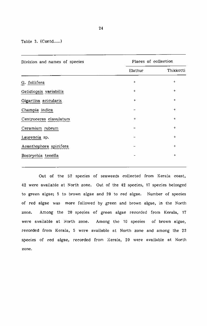
24

Table 3. (Contd.....)

Division and names of species Places of collectionElathur ThikkottiQ. foliifera + +

Gelidiopsis variabilis + +Gigartina acicularis + +Champia Egg - +Centroceras clavulatum + +Ceramium rubrum - +Laurencia sp. - +Acanthophora spicifera — +Bostrxchia tenella - +

Out of the 52 species of seaweeds collected from Kerala coast,

42 were available at North zone. Out of the 42 species, 17 species belonged

to green algae; 5 to brown algae and 20 to red algae. Number of species

of red algae was more followed by green and brown algae, in the North

zone. Among the 20 species of green algae recorded from Kerala, 17

were available at North zone. Among the 10 species of brown algae,

recorded from Kerala, 5 were available at North zone and among the 22

species of red algae, recorded from Kerala, 20 were available at Northzone.

25

Table 4. Number of orders, families, genera and species of seaweedsrecorded from North zone.

Chlorophyta Phaeophyta Rhodophyta Total

Orders 4 2 6 12Families 6 2 1 1 19Genera 10 4 15 29Species 17 5 20 42Seaweeds exclusive to North zone

Chaetomorgha linum

Sgongomorgha indica

Cladophoropsis zollingeri

Caulerga fastigiata

Boodlea comgosita

§Qathoglossum asperum

Turbinaria ornata

Grateloiggia comoronii

Hxgnea sp.


Chamgia indica

Ceramium rubrum

Bostrychia tenella

13 species of algae were found to be exclusive to North zone of

Kerala, out of which 5 species belonged to Ch1orophyceae,2 to Phaeophyceae,

and 6 to Rhodophyceae.

4.3.2 Seaweeds from South zone of Kerala coast

Table 5. Seaweeds from South zone of Kerala coast

. . . . Place f e t'oDivision and names of species 0 C011 C 1 nVarkala Mullur

DIVISION : CHLOROPHYTAfl fasciata + +y_. lactuca + +Enter-omorpha compressa + +Chaetomorpha antennina + +Cladophora glomerata — +Q. fascicularis - +Cladophora sp. + +Bryopsis plumosa — +Caulerpa i'acemosa — +Q. peltata - +_(_3. scalpelliformis - +Q. sertu1arioi>g_e_5 - +Valoniopsis gchynema + +

27


Division and names of speciesPlace of collection

Varkala Mullur


C " os ora minima

Dictyota bartayresiana

2. dichotoma

Padina gymnosgora

E. tetrastromatica

Sargassum tenerrimum

§. wightii

Turbinaria conoides

DIVISION : RHODOPHYTA


Acrochaetium sp.

Gelidium gusillum

Amghiroa fragilissima

flfliulisGratelougia filicina

Q. lithoghila

Hygnea musciformis

_Ii. valentiae


28

Table 5. (Contd...)

Division and names of species Place Of C011€0ti0nVarkala MullurQ. foliifera + "

Gelidiopsis variabilis + +Centroceras clavulatum + +Spvridea filamentosa - +Laurencia sp. - +Acanthcghora spicifera - +

Out of 52 species of seaweeds collected from Kerala coast, 37

were available at South zone. Out of the 37 species, 13 belonged to green

algae, 8 to brown algae and 16 to red algae. Rhodophyceae were more

abundant in the South zone, followed by Chlorophyceae and Phaeophyceae.

Out of the 20 species of green algae recorded from Kerala, 13 species

were available at South zone, out of the 10 species of brown algae, 8

were available at South zone and out of the 22 species of red algae 16were available at South zone.

Table 6. Number of orders, families, genera and species of seaweedsrecorded from South zone.

Cholorophyta Phaeophyta Rhodophyta TotalOrders 3 3 5 1 1Families 5 3 9 17Genera 7 5 13 25Species 13 8 16 37

29

Seaweeds exclusive to South zone

Caulerga racemosa

Chnoosgora minima


Sargassum tenerrimum§Turbinaria conoides

Amghiroa fragilissima

Sgxridea filamentosa

8 species of seaweeds, 1 belonging to Chlorophyceae, 5 to Phaeo

phyceae and 2 to Rhodophyceae were found to be exclusive to South zone

of Kerala.

4.3.3 Seaweeds from Central zone of Kerala coast

DIVISION : CHLOROPHYTA

Enteromorpha compressa

E. f lexuosa

Chaetomorpha antennina

Br-yogsis glumosa


Nil

DIVISION : RHODOPHYTA

Acrochaetium sp.

J ania rubens

30

Grateloupia filicina

_C_5. lithophila

Centroceras clavulatum

Out of the 9 species of seaweeds collected from Central zone,

4 species belonged to Chlorophyceae and 5 to Rhodophyceae. No Phieophyceaen

member was present.

Table 7. Number of orders, families, genera and species of seaweedsin Central zone.

Chlorophyceae Rhodophyceae TotalOrders 3 3 6Families 3 4 7Genera 3 4 7Species 4 5 9Enteromorpha flexuosa was found to be exclusive to Central zone of Kerala.

Table 8. Number of seaweed species recorded from different zones ofKerala.

Division Number of seaweed species recorded from differentzones of Kerala

South zone Central zone North zone

Chlorophyta 13 4 17Phaeophyta 8 0 5Rhodophyta 16 5 20Total number ofspecies 37 9 42

31

Thus number of seaweed species was maximum in North zone (42 species),

followed by South zone (37 species) and Central zone (9 species). Number

of species of Chlorophyceae and Rhodophyceae in North zone was greater

than in South zone. But number of species of Phaeophyceae was greater

in South zone than in North and Central zones. In Central zone 4 species

of Chlorophyceae and 5 species of Rhodophyceae were present, but no

Phaeophycean member was present.

32

4.4 ZONATION PATTERN OF SEAWEEDS ALONG KERALA COAST

During the course of the present investigation, a definite zonation

pattern was observed with regard to several species of seaweeds. Ulva

fasciata, E. lactuca, Chaetomorpha antennina, Enteromorpha compressa,

Prophyra kanyakumariensis, Grateloupia lithophila, 9. filicina and Centroceras

clavulatum were found to grow on the rocks of the upper littoral zone.

Rocks exposed to heavy breakers and swells harboured algae with strong

holdfasts like Chaetomogma antennina, Porphyra kanyakumariensis, Grateloupia

spp., Gracilaria spp., Spyridea filamentosa, Sargassum spp. and Chnoospora

minima. Hypnea valentiae, Acanthophora spicifera, Laurencia sp. and

Caulerpa scalpelliformis were observed in the deeper regions of the mid

littoral zone at Mullur. At Mullur, Caulerpa peltata was found to grow

on the leeward side of the rocks in the mid littoral zone which is constantly

covered and uncovered by water. At Thikkotti and Mullur, Caulerpa

sertularioides was found to grow on sandy bottoms of the sea, at about

1 m depth. At Elathur, this species was found to grow on the sides of

rock pools in the mid littoral zone which was exposed for the major part

of the day. At Mullur, the lower littoral zone was inhabited by species

of Sargassum, Spyridea, Gracilaria and Dictyota which cannot tolerate long

exposures and dessication. Sargassum spp. always grew on the seaward

side of the wave exposed rocks. Species of Enteromorpha were found to

grow in almost all the aquatic biotypes. At Elathur, Enteromorphaintestinalis was found to grow in a highly polluted coconut

33

retting area. At Varkala, Enteromorpha occupied the rocks which were

periodically covered and uncovered by sand.

At Saudi, a definite pattern of horizontal zonation of seaweeds

was observed (Fig.2). In the Central part of the station two distinct zones

of seaweeds were found to exist. The first zone was occupied by species

like Grateloufl lithophila, Q. filicina and Centroceras clavulatum. The

second zone was occupied by only Enteromorpha compressa. On either

side of the Central zone, Chaetomog>ha antennina and Centroceras clavulatum

showed a mixed growth.

At Varkala also a definite horizontal zonation was observed (Fig.3).

The first few rocks near the entrance to the beach were occupied by

Enteromorpha. This area showed marked seasonal changes in the topography,

characterised by the covering and uncovering of rocks by sand. After

this zone there was a definite zone of Ulva lactuca, Enteromorpha compressa

and Chaetomorpha antennina. This zone is followed by a zone with mixed

growth of Grateloupia lithophila, Q. filicina, Ulva fasciata, H. lactuca,

Chaetomorpha antennina and Centroceras clavulatum.

OCON o=oN econ OCON

unzoootcoo o.._EoEo.2cm anzouozcoo ngouozcoo

o.._n:oEo—oo.._o o_m:o_o.o.0 2.m.os22Eo

N .9...

_o:<m ._.< om>mmmmo mommzsqmm mo zo:<zoN n_<._.zON_mOI

34

4.5 DENSITY OF SEAWEEDS IN DIFFERENT STATIONS ALONG KERALACOAST

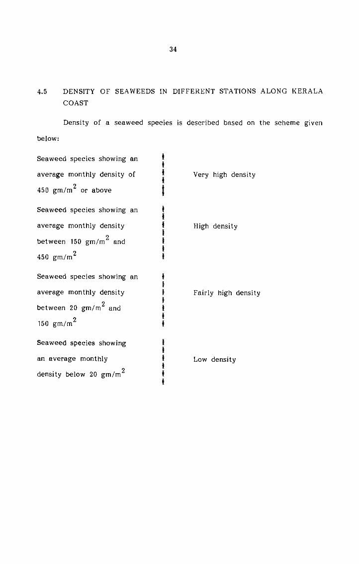
Density of a seaweed species is described based on the scheme given

below:

Seaweed species showing an

average monthly density of

450 gm/m2 or above


average monthly density

between 150 gm/m2 and

450 gm/m2


average monthly density

between 20 gm/m2 and

150 gm/m2

Seaweed species showing

an average monthly

density below 20 gm/m2-$1:-fir-O-no-vi-Quuc-I -en-3:312:-9-we-the-I -on-¢u-on-Q-:1-QII-Q-I31 -junta-Q1-311$:

Very high density

High density

Fairly high density

Low density

35

v.u.u.Ev

z. z I 9

uwmnm.muuu..u.um.”m.._.mmm.....u.u.u.www.n..,w.u ww .u.u..L,w..c s.,.r., ..:”__.....u,...:2 . 9: :5 S. S. 3 . . . . . . . =8 . . 2. S . . . 3. . 3 . . . S . 3 2: 8 .5...

2: . E: S. 9... . 3. 3. 2: . . . . . . 3. . . E. . . . 2: . . . . 3. =2 2. 2. .8:£2 2: 2: 3 . 3. .3 . . . . 2. . . . e... 2 . . S. . . . 3. . 2: em. 3 .322.: . mp =2 2: . 2: =2 . . . . . . 2: . . . 2: 2: . . S. . . . . =2 . 3. c2 3 .20

$2 . . 3n 2: . =2 . . . . .3 . n S. . . . . 2: . . fin . . . . fin . 2: 9: 2 dam2.3 . . =3 . 2; =2 . . . . . an ...: . . . . =3 . . Sn . o . . 2. 3. 3... in 2 .....<

S: . . 3. .5 en. . . . . an on . . . . =2 . . SN . . . 3... .: =3 3.. on ._=...33 . . in an eon . . . . . . an on . . . . . . . =2 . . . . =2 . . 2: 2 .25..

...:: . . can an 2: S . . . . . . . E. . . 2. . . . . S. . . . . . E S. ...: 2 5.:fivu . . can :3 8... .3 up . . . . . . Sn . Sn . . . . . 3 . . . an . . . . S. 3 ..a<82 . S. 2.: 2. E: .: . . . . . . Sn . . 2: =2 3 . 2. . S. . . 2: S 2: 2 2: 2 ..=.:3% . . 5: e2 25 E: 2: . . . . . Se . . 2: . E... . . 2: Sn . . . 2. . E: e3 .3 5!.

S3 . . 2; .5 So . 2: . . . . . . 8.... . . 2: . =3 . . SS 8. . . . 8. . . 8.: 2 ...c..

2.2 . 9! =8 . 8.: :2 :8 . . . . . 2.2 . S. . . . . . 2: . . . . 2: . So . 2 doc82 . . =2 3. 2: 23 2; 2:. 25 . . . . . Se . =8 . . :3 . . 2:. . . . . . 2: . =2 =8 S .32

22 . . 2: 2; . =3 . . . . . . . . 2: . . . . 9.: . . 2: . =2 . . . 2: . . Sn 2 .3083 . . 2: 2: . 2: . . . . . . . . 23 . . 8. . es: . . 8.: . . . . . 2: . S. 33 2 Arm

2.: . . 2: 2. S 8- Se . . . . S . . Sn . . . . 2: . . 8: . 2. . . . 8. . :2 =2: 8 .!<anew . 2: . . So . . . . . . o B 2: . . . . co. . . . . . . . . . . . 2:: 2 .1...

8: . . 2.: . . =3 . . . . . . . Se . . . . . . . 2: . . . . . 2: . . 2.. 8 .5...

S: . 2: 3. 8.. . . . an an :3 . . SN . . 2 . . 2.. 2: . =3 . . . . 3 . 2 . 3 4.:2.3 2.. 2: . 8. . . . . . . . . 8. . . E: . . . . . 2. 2: 2: . . 2: . . =8 3 .k_<3: . . 2: 3. . 2.... =3 . . . . . . . :2. . . 2: . . . . . . . . . . 2; . 3 .._..z33 . . 3.. .7. 2: _....u E... . . 2 . of . . 8. . . 2: . =2 . . . . . . . E3 =3 S .9:

.=_!u=._

\3__.v...._.m.% 2 S : 2.. 3 -N Z 2 2 3 2 S : 2 2 -_ E 2 m. w n. S 2 m c F 0 m w n N _

.~E\Eu. .25: .- Gaoluan B 3.5.»: o.u_n-._.

n=:=s_ _¢ utoolcbw U .:.a.....: ..

Species

Species

Species

Species

Species

Species

Species

Species

Species

Species

Species

Species

Species

Species

Species

Species

Species

Species

Species

Species

Species

Species

10

11

12

13

14

15

16

17

18

19

20

21

22

36

INDEX TO TABLE 9

Ulva fasciata

E. lactuca

Enter-omorpha com pressa


Cladophora glomerata

Q. fascicularis

Cladophora sp.

Brxopsis plumosa

Caulerpa racemosa

Q. peltata

Q. scalpelliformis

Q. sertularioides

Valoniopsis pachynema

Chnoospora minima

Dictyota bar-tayresiana

Padina gxmnospora

_I:. tetrastromatica


§. wightii


Achrochaetium sp.

Gelidium pusillum

37

INDEX TO TABLE 9. (Contd...)

Species 23 Amphiroa fragilissima

Species 24 J_Bl'£l£Species 25 Grateloupia filicina

Species 26 E. lithophila

Species 27 Hypnea valentiae

Species 28 Gracilaria corticata

Species 29 Gelidiopsis variabilis

Species 30 Centroceras clavulatum

Species 31 Spyridea filamentosa

Species 32 Laurencia sp.

Species 33 Acanthophora spicifera

* denotes that the species was available in traces only and hence, density

could not be estimated.

- denotes that the species was not available during that month.

38

At Mullur, Ulva fasciata showed the highest density (690.63 gm/m2).

Other seaweeds that showed very high densities were Sargassum wightii,

Gracilaria corticata and Spyridea filamentosa. Ulva lactuca, Chaetomorpha

antennina, Caulerpa peltata, Chnoospora minima and Centroceras clavulatum

showed high densities. Bryogsis plumosa, Caulerpa racemosa, Valoniopsis

pachynema, Padina gymnospora, _P_. tetrastromatica,Porphyra kanyakumariensis,

Gratelougia filicina, Q. lithcfliila, Hypnea valentiae, Gelidiopsis variabilis

and Laurencia sp- showed fairly high densities. Species that showed low

densities at Mullur were Enteromorpha compressa,Cladophora glomerata,

Q. fascicularis, Cladophora sp., Caulerpa scalpelliformis, E. sertularioides

Sargassum tenerrimum, Achrochaetium sp., Amphiroa fragilissima and Jania

rubens.

Table 10. Seasonal density of different divisions of seaweeds at Mullur.

Average seasonal density gm/m2AlgalDivision Pre monsoon Monsoon Post monsoon

GreenAlgae 1026.25 2090 1343.75BrownAlgae 1203.13 377.50 1218.75RedAlgae 1815 1301.88 1537.50Seasonalseaweeddensity 4044.38 3769.38 4100

39

From Table 10 we can draw the following conclusions:

At Mullur,

Green algal density was highest during monsoon followed by post

monsoon and a comparatively low density was recorded during pre

monsoon.

Brown algal density was high during both pre and post monsoon

but comparatively low during monsoon.

Red algal density was highest during pre monsoon followed by post

monsoon and comparatively low during monsoon.

During pre monsoon and post monsoon red algae showed the highest

density.

During monsoon, green algae showed the highest density.

Both brown and red algae showed a reduction in their densities

during monsoon.

Algal density was maximum during post monsoon followed by premonsoon and monsoon.

Table 11.

40

Seasonal density of some seaweeds from Mullur

Names of seaweeds

Average seasonal density (gm/m2)

Pre monsoon Monsoon Post monsoon

E fasciata 406.25 1196.88 4.68-75H. lactuca 153.13 121.25 268.75Chaetomorpha antennina 95 205.00 300Caulerga gee 221.88 343.75 281.25Chnoosgora minima 118.75 125 271.88fim gymnosgora 321.88 21.25 59.38Sargassum 693.75 231.25 718.75Gracilaria corticata 562.50 497.50 475Centroceras clavulatum 228.13 149.38 250Sgxridea filamentosa 762.50 243.75 393.75Hygnea valentiae 137.50 112.50 168.75Porphyra kanyakumariensis 0 193.75 9.38Gratelougia lithoghila 43.75 0 112.50Laurencia sp. 27.50 0 34.38

. v,.:.=.Kw.

41

Z J I r. I C. 7. . zwaom m .. H .» u z W .. . . W V. m N . u .n .1 m .m n m _.,_=._.,...=...m.. ..,.. m u -. u u u u u n. u u m u. m n -. ..:..2

=3. =2 . . . . . =2 . . . . . =2 . . . . . === . === . == :5.=3. =3 . =3 . . . . 3 === 2 8:8: =3 . === . . . . 8. === . 3 >02as . . . . . . . . . . . . E . =3 =3 2 J90Ev . . . 2. =2 =3 3 don==... 2. . . . . . 2 3 =2 =2 =. .....<=3. . . . ==n . . . . . =2 3... 2 3....=9. ==_ 2. 2. . =3 . . . =3 3... . 2 .15..=3. . . =8 . . . . . . =3 . . =2 8 .>.us_=3 2: <0 =2 . . . S ...=<c==. . 3 2.. . - =3 3 =3 =_.._ ac ._..£:2 =2 is =2 . =3 ==_ . =3 . . . . =..._ ==_ =2 2 .=...._83 =3 . . . . === . <u ==== <0 . Sn ==m . ==.: == .5...=3. :2." . . === . . 9 (U . . . 2 as no ....0C8: === . === . . . . . ==. =3 8 :3222 . . . . . === . =2 =2 === =3 8 . toSS 2 3 3 . . 2 . . ==... 3- 8. =3 2 don=2" =3 . . . . =: . . =2 . === =2 8. =8. 3 .w.<===u . . . . . . ===_ . . . . =9 . S5 8.: 3 >._.._.can 2: . E: . . . . . . . .5: . . an 25..con. . . =3 . . . . . . . . === . on 552.. =2 . . . . . =2 =2 =2 .3 .x_<ea: . . . =3 . . . =3 ecn . as .32in . ==_ =3 =3 =3 . === . . . . . . . . . . 3 ==... . =2 .3 .9:

5.E.__a.n 2 : 3 2 2 2 2 2 : 2 2 ._ 2 = = =. _. ... v = N _

5.1!»

.~=.:E3 .._!t¢> .1 Jvuol-on 3 >_..u:X.._ 2&3-._.

¢_Stu> .1 fivoslcun 3 3.25 n.....v

Species

Species

Species

Species

Species

Species

Species

Species

Species

Species

Species

Species

Species

Species

Species

Species

Species

Species

Species

Species

Species

Species

10

11

12

13

14

15

16

17

18

19

20

21

22

42

INDEX TO TABLE 12

Ulva fasciata

E. lactuca



Cladophora sp.


Chnoospora minima

Dictyota dichotoma


S. wightii

Turbinaria conoides

Porphira kanyakumariensis

Achrochaetium sp.ESGrateloupia filicina

Q. lithophila

Hypnea musciformis

fl. valentiae


Q. foliifera

Gelidiopsis variabilis


43

INDEX TO TABLE 12. (Contd...)

"‘ denotes that the species was available in traces only and hence, density

could not be estimated.

— denotes that the species was not available during that month.

CA denotes that the species was collected as cast ashore weed and hence

the quantity could not be estimated.

44

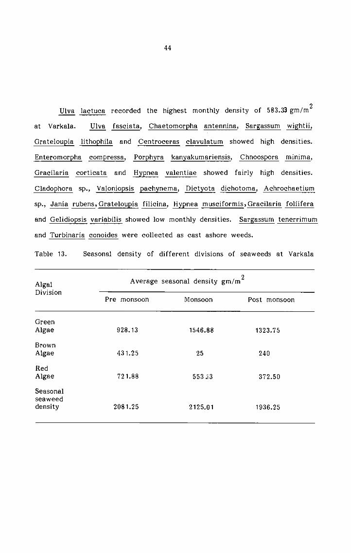
Ulva lactuca recorded the highest monthly density of 583.33 gm/m2

at Varkala. Ulva fasciata, Chaetomorpha antennina, Sargassum wightii,

Grateloupia lithophila and Centroceras clavulatum showed high densities.

Enteromorpha compressa, Porphyra kanyakumariensis, Chnoospora minima,

Gracilaria corticata and Hygnea valentiae showed fairly high densities.

Cladoghora sp., Valoniopsis pachynema, Dictyota dichotoma, Achrochaetium

sp., Jania rubens,Gratelou;3ia filicina, Hygnea musciformis,Gracilaria foliifera

and Gelidiogsis variabilis showed low monthly densities. Sargassum tenerrimum

and Turbinaria conoides were collected as cast ashore weeds.

Table 13. Seasonal density of different divisions of seaweeds at Varkala

Algal Average seasonal density gm/m2Division Pre monsoon Monsoon Post monsoon

GreenAlgae 928.13 1546.88 1323.75BrownAlgae 431.25 25 240RedAlgae 721.88 553.‘i3 372.50Seasonalseaweeddensity 2081.25 2125.01 1936.25

45


At Varkala,

1. Green algal density was highest during monsoon, followed by post

monsoon. Pre monsoon recorded comparatively low density of green

algae.

2. Brown algal density was maximum during pre monsoon followed by

post monsoon. During monsoon brown algal density was very low.

3. Red algal density was high both during pre monsoon and monsoon

but comparatively low during post monsoon.

4. During all the seasons green algae showed the highest density.

5. Monsoon season recorded the maximum seaweed density followed

by pre monsoon.

Table 14. Seasonal density of some seaweeds at Varkala

Average seasonal density (gm/m2)Names of seaweeds


E fasciata 31.25 393.75 131.25E. lactuca 418.75 662.50 668.75Enteromorpha compressa 21.88 31.25 340Chaetomorpha antennina 356.25 459.38 133.75Centroceras clavulatum 143.75 37.50 277.50Porghyrakanyakumariensis 0 359.38 0

46

nuruwnnM .,l. .u ,_ . .m .m. m . . M -|v M 1 .u .0 m m n W. m ;.._._u..“W -. .u M H ... N . H .u W H. ,.. H u ._ N n :__.g._.fi2.... 5 3 =2 2: 2: . . =2 . . 2 2: 2.. 8 ......2.: . 2.... . . 2 . . . . . . . 2: 2: 2 ...»:2.2 2... 2: . S. . . . . . . . 2: . S .32can . . . . . . . . . . 2: =3 . . an ..uo2: 2: .. . . =3 8. 3. . . . . . . . 2: . 2: 2 Ana

2% 2., . 2: . . . . . . . . 2: 2: S 8. 2. .?<2.. 2: 2: 23 . . . . . at E. 3. 2 ......So 2: . SN . 2... . . . . . 2: . . .3 .5...32 2... E . . 2; =2 2: . . . . . . S. . . fin . . 2. 2.:=3 . 2: 2: 2. 2: . . . . . . . 2: . 2 .x_<Sm .... . . 2: S . . . . . . . 25 . . S .3 ...:2.2 SN :2 2: Sn . 2: . . 23 . 23 . 2: 2 .oo..

2:. 2: 2: . . . . . . . . . . 2:” . . . 2. ......econ . . . =2: . . . . . . . . . . 2:: =2: 8 do:23... 2: . 2.3 . . . . 2.: . . . . . . . .33 . ... .322: . . . . . . . . . . . . . 2: 2: . . 2. .3032.. 2 2: 2.: 2.: . . . . . . 3 . 2:. 8. 2: . 8 dam

2.2 . . . 2:: . . . . .2. . . . 2:: 2... =2 . ... .!<2: 2: . . an 3.. . . . . . . =2 S . . S ......2.2 . . . 2...: . . . 2: . . . . . 8 .5...=3 . . 2.. . . 2: . . 2 ......S3 2: . 2:: SS 2:: . . 2...: S .....<2.2 . . 2:. 2.. . . . . . . 2.... ... ...:2: 2.. 2: . . ...: SN :2 . . S . . . 2.. 2: . . 2: . 2 2. .. do.

?€.l§_.uv.-H : 5.. 2 2 : 2 m. : 2 2 : 2 o . .. u ... q n u _

.n::Eu. 55:2 .1 xhulaou 3 E29: ..._.w_au._.

....:.._u E ...t.lu& U _:.z...._ .24

47

INDEX TO TABLE 15

Species 1 Ulva fasciata

Species 2 E. lactuca

Species 3 Enteromorpha intestinalis

Species 4 Chaetomorpha antennina

Species 5 Cladophora fascicularis

Species 6 Cladophora sp.

Species 7 Caulerpa sertularioides

Species 8 him gymnospora

Species 9 E. tetrastromatica

Species 10 Porphyra kanyakumariensis

Species 11 Achrochaetium sp.

Species 12 Gelidium pusillum

Species 13 Jania rubens

Species 14 Grateloupia comoronii

Species 15 Q. filicina

Species 16 Q. lithophila

Species 17 Gracilaria corticata

Species 18 Q. foliifera

Species 19 Gelidiopsis variabilis

Species 20 Gigartina acicularis


* denotes that the species was available in traces only and hence the

density could not be estimated.


48

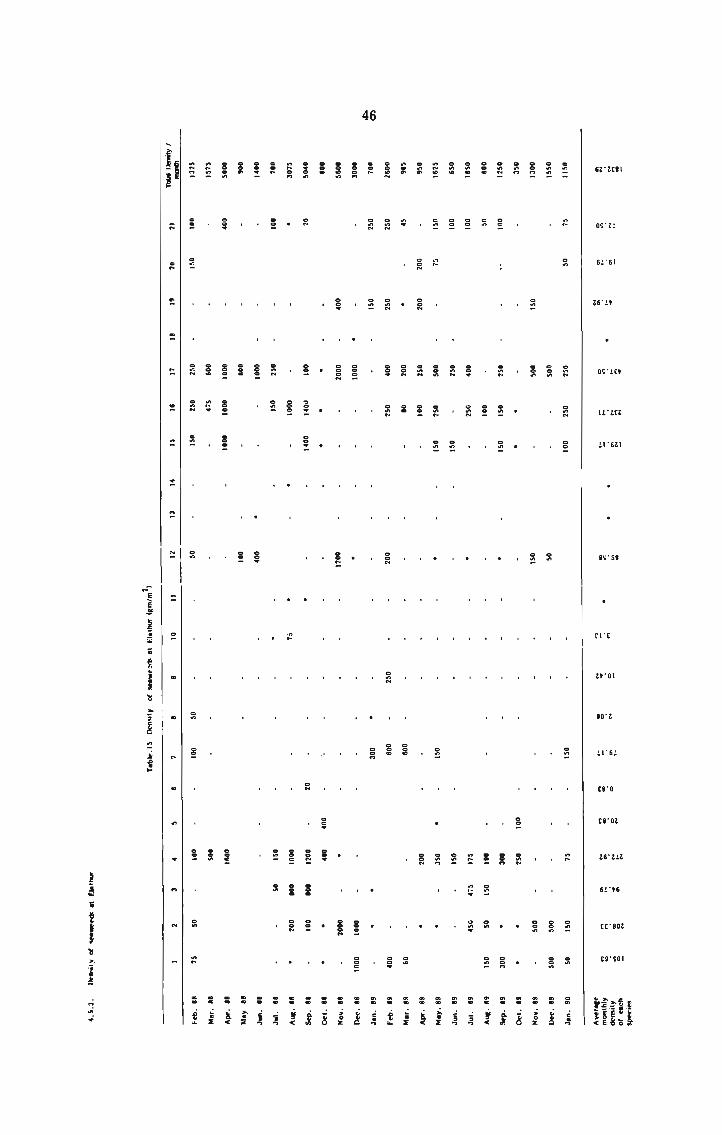
At Elathur, Gracilaria corticata recorded the highest monthly density

of 437.50 gm/m2. Ulva lactuca, Chaetomorpha antennina and Gratelougia

lithoghila also recorded high monthly densities. Ulva fasciata, Enteromorpha

intestinalis, Cladophora fascicularis, Caulerpa sertularioides, Gelidium gusillum,

Gratelougia filicina, Q. lithophila, Gelidiopsis variabilis and Centroceras

clavulatum recorded fairly high monthly densities. Cladophora sp., Padina

tetrastromatica, E. gymnospora, Porphyra kanyakumariensis and Gigartina

acicularis recorded low monthly densities.

Table 16. Seasonal density of different divisions of seaweeds at Elathur

Algal Average seasonal density (gm/m2)Division


GreenAlgae 626.25 550 1171.25BrownAlgae 37.50 D 0RedAlgae 1121.88 800 1190Seasonalseaweeddensity 1785.63 1350 2361.25


At Elathur,

1. Green algal density was maximum during post monsoon. Pre monsoon

and monsoon recorded a comparatively low density of green algae.

49

2. Brown algae were observed only during pre monsoon.

3. Red algal density was high both during pre and post monsoon but

comparatively low during monsoon.

4. Algal density was highest during post monsoon followed by pre mon

soon. Monsoon recorded a comparatively low algal density.

5. During all the seasons, red algae showed the highest density.

Table 17. Seasonal density of some seaweeds at Elathur

. 2Names of seaweeds Average seasonal density (gm/m )


E fasciata 73.13 18.75 225E. lactuca 25 87.50 512.50Chaetomorpha antennina 309.38 240.63 268.75Caulerga sertularioides 218.75 18.75 0Gelidium gusillum 31.25 62.50 175Gratelougia filicina 156. 25 37.50 193.759- lithoghila 300.63 218.75 193.75Gracilaria corticata 368.75 400 543.75Centroceras clavulatum 140 62.50 15

50

3.8.?so-0N Z Z l I .9 fileW . W ..,.. ..., W .. ... .. . M 1 ,. H 1 .n. .u .u. .... .. .5 m .,n_.fi

n u. u .... .u. u w. u w. u u w .u w u M .o. u ..,. u u _.

9... . . . . . . 2. . . . . . . . e2 e2 . . 22 . . . . 2 ..=_.2: - 2. . . - . . . . 2: . . 92 an .8:8- . S u . ea. . an . . an :9. . . . . an .32

an . 2 . . . . . . . . . - . 2: . . . . e2 :2 2 .302:. . 2: . . . . . . . . 2: . . =3 :2 2 damat . Sn . . . 2: . . . . . =2 . 2. an .!<

2: . Sn . =3 . . . . 2. . . 2: Sn 8 ._=_.2- 2. 2 2 . . . . . . . 2. 2. . 8 .§..22.. can . =2 2 . :2 . . . Sn . 2... as - - 25 2. . . 2 »-22.: =8 . . . =2 . . . . Sn . . . S... . 2 ....<2; 2» . . . .3. . . . . 2. 2 . . =2 . . . .3 .._.z2: Sn :2 . =2 . . . . 3... . . . 2. . . 2. 53.

S: . . - 3. . =2 . - . . . - . 8... ._2 S. . 2 ..=_.32 . 8. . . . . . . . . . 2: . . . coo. . . . 3 can23.. . 2: 2; . 2:: . 82 . . 2. 82 . 2. 3.: . 2 . . . . . . . B .32

2.: . . . . . E: . . . . . . . . . . . - . 92 - 3- 2: 2 ....o:2 . S. . . 2. . . . . .. . 2 E: 2: so damas . . 2 . . . . . . . . . . =2 :2 2 2 S .!<

2: . 2 =2 . . . . 2 . . . 2 2 . . :2 . 2 . 3 :2.2.2 . 5:. . . . 3 3 8.: . . . =2 . S .5...:3 =2 . . . . . =2 . . . .3. . . S .3:3: . . 3 . . .3. . 8. . . =2 2 .....<2: 2. . - . =3 . =2 . - . . 3 : .....:mt . =2 . . . . 22 . . . . . . . =2 . . . 2 . . . . . 3 £1

2 2 2 2 : 2 2 2 : ..: E : 2 2. : 2 . .. e m w n 2 _

£EE5 _:9____.:. 3 ‘van!!! .3 3.9.»: 5.93:...

_:e_.__..._. E .000!-I I Eli... 45..

Species

Species

Species

Species

Species

Species

Species

Species

Species

Species

Species

Species

Species

Species

Species

Species

Species

Species

Species

Species

Species

Species

10

11

12

13

14

15

16

17

18

19

20

21

22

51

INDEX TO TABLE 18

Ulva fasciata

E. lactuca

Enteromorpha intestinalis


Spongomorpha indica

Cladophora glomerata

Cladophora sp.

Cladophoropsis zollingeri

Bryopsis plumosa

Caulerpa scalpelliformis

Q. sertularioides

Boodlea composita


Gelidium pusillum

Jania rubens

Grateloupia comoronii

Q. litho hila

Hypnea valentiae


G. foliifera

Gelidiopsis variabilis


52

INDEX TO TABLE 18 (Contd...)

Species 23 Champia indica


Species 25 Bostrychia tenella

* denotes that the species was available only in traces and hence the



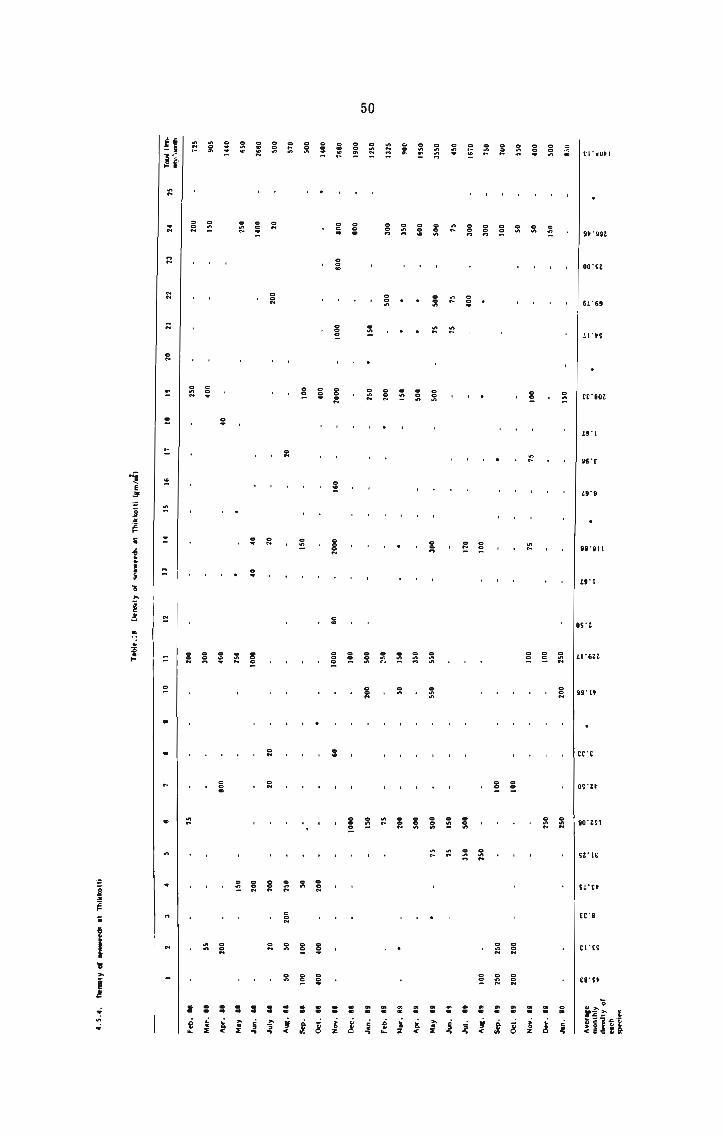
At Thikkotti, 12 species of seaweeds, 3 belonging to green algae, 4 belonging

to brown algae and 5 to red algae were collected as cast ashore weedsand hence their densities could not be estimated.

Table 19. Cast ashore weeds and their months of occurrence at Thikkotti.

Names of seaweeds Months of occurrence

Chaetomorpha linum

Caulerpa f astigiata

_c_. peltata

Dictyota dichotoma

Padina tetrastromatica


Turbinaria ornata

Hypnea musciformis

Hypnea sp.

Ceramium rubrum

Laurencia sp.

Acanthophora spicif era

January and February

January, February and July

January and May

November and March

November and March

November and March

February and April

November and December

January and March

November

February and March

January - May, September,November

53

At Thikkotti, Centroceras clavulatum recorded the highest density

of 266.46 gm/m2. Cladgmora glomerata, Caulerpa sertularoides and

Gracilaria corticata also showed high monthly densities. Ulva fasciata,

E. lactuca, Chaetomorpha antennina, Spongomorpha indica, Cladophora sp.,

Caulerga scalpelliforrL$, Gelidium pusillum, Gelidiopsis variabilis, Gigartina

acicularis and Chamgi indica showed fairly high monthly densities.

Table 20. Seasonal density of different divisions of seaweeds from Thikkotti.. 2Algal Average seasonal density (gm/m )Division


GreenAlgae 644.38 693.75 627.50RedAlgae 523.75 658.75 1076.25Seasonalseaweeddensity 1168.13 1352. 50 1703.75


At Thikkotti,

1. Green algal density was highest during monsoon followed by premonsoon and post monsoon.

2. Red algal density was highest during post monsoon. Monsoon and

pre monsoon recorded comparatively low densities.

3. During pre monsoon and monsoon green algae showed higher density

than red algae.

54

4. During post monsoon red algae showed higher density than green

algae.

5. Algal density was highest during post monsoon followed by monsoon.

Pre monsoon recorded the lowest algal density.

Table 21. Seasonal density of some seaweeds at Thikkotti



Ea fasciata 0 18.75 118.75E. lactuca 31.88 8.75 118.75Chaetomorpha antennina 0 100 31.25Cladoghora glomerata 156.25 143.75 156.25Caulerpa sertularioides 300 225 162.50Gelidium Qusillum 0 72.50 278.13Gracilaria corticata 237. 50 62.50 325Gigartina acicularis 62.50 146.88 0Centroceras clavulatum 200 355.63 243.75

55

m ..., m R . . m .n m

M 3 m n M M ..u. H uu.:....<.5. 2: 2. . . . . .3. . 3 3 .8:3.. .5. E: . . 2. . S .3:2. .5. 2... . . 2. . 2. ...5.....v =.: E: . . =2 . 2: an .92..E: 2.. . . . 2.” 2.. 2 .?<2.... ...: =2 . . . . . 2. 3 ._._..

=3 2: . . . . . 2: . =2 .3 .5...3... .=: . . 2: SN .3 ...=...=2. 3 . . 2.. 2... E. .._._<2.» =3 3 . =3 2 3 .._.i_=2. is . 2.... . . .5... . . 2. .3...2.... =3 . . . . . . 3.: 2 .5...

....._..u 25 . ....: . . 3.: 2 .2:.=:. . . 2: . . =2 5. ..:.z5:... .5... . ..._§ :3 2.... =5. .3 ....:=8. . . .5... . . . 2:. . .5. 2. den22. 3 8.. . . ex: . .5. on .....<3.: . . . . =3 . E; 2. .__...2.: . . . . . . 8.: 2... 2... 3 .5...

2:: =3 . =3 . . . S. . 2: 8 :23.2 .2... . . . 3.: . 3 .....<9...: 2: :3 Sn . . . 2; =2 S ..=_...:3. .3. S. S. . 23 . 3 .9:3... 3 Sn .3... . . . 2:: . . S ..=..

..Eo_.:.:.El.. _-5+ g n .. u ... o n N _

_wE\E5 ascw .- ufiooluuv, 3 .:.U:X_ 3.03:...

53cm 3 1.2.9310». 3 3.2.0:

5.“.

Species

Species

Species

Species

Species

Species

Species

Species

Species

2

56

INDEX TO TABLE 22

Enter-omorpha compressa

_E_. f lexuosa


Bryopsis plumosa

Achrochaetium sp.

Jania rubens

Grateloupia filicina

Q. lithophila


* denotes that the species was available only


in traces and hence the


57

At Saudi, Chaetomorpha antennina recorded the highest monthly

density of 536.46 gm/m2. Enteromorpha compressa, Grateloupia filicina

and Centroceras clavulatum recorded high monthly densities. Enteromorpha

flexuosa, Jania rubens and Grateloupia lithophila recorded fairly high den

sities. Bryogsis glumosa and Acrochaetium sp. were found only in traces.

Table 23. Seasonal density of different divisions of seaweeds at Saudi

. 2Algal Average seasonal density (gm/m )Division


GreenAlgae 765.63 1000 609.38RedAlgae 558.75 302.50 926.25Seasonalseaweeddensity 1324.38 1302.50 1535.63From Table 23 we can draw the following conclusions:

At Saudi,

1. Green algal density was maximum during monsoon followed by pre

and post monsoons.

2. Red algal density was maximum during post monsoon followed by

pre monsoon. During monsoon the density was comparatively low.

3. During both pre monsoon and monsoon green algal density was more

than that of red algae.

58

4. During post monsoon red algal density was more than that of green

algae.

5. Algal density was maximum during post monsoon followed by premonsoon and monsoon.

Table 24. Seasonal density of some seaweeds at Saudi



Enteromorpha compressa 65.63 406.25 193.75Chaetomorpha antennina 700 493.75 415.63Gratelougia filicina 206.25 181.25 523.13E. lithoghila 131.25 12.50 68.75Centroceras clavulatum 221.25 121,25 25250

Table 25. Seasonal density of different algal divisions along Kerala coast

Average seasonal density (gm/m2)Algal division


Green Algae 798.13 1176.13 1015.13Brown Algae 334. 38 80.50 291.75Red Algae 948.25 723.25 1020.50Seasonal seaweed density 2080.76 1979.88 2327.38

59


Along Kerala coast,

1. Green algal density was highest during monsoon.

2. Brown algal density was highest during pre monsoon.

3. Red algal density was highest during post monsoon.

4. Among seasons,post monsoon recorded the highest density.

4.6 FREQUENCY OF OCCURRENCE OF SEAWEEDS ALONG THE KERALACOAST

It was observed that the frequency of occurrence of each species

of seaweed (number of months during which a particular species was obser

ved) fell in one of the three classes described below:

Species showing very high frequency of occurrence (taken as those

species that occurred for 15 months or more, in the present study).

Species showing high frequency of occurrence (taken as those species

that occurred for 8 months or more but less than 15 months in the present

study.

Species showing low frequency of occurrence (taken as those species

that occurred for less than 8 months in the present study.

Based on the above described scheme, the seaweed species showing

very high, high and low frequencies of occurrence along the different zones

of Kerala coast are represented in Tables 26-28.

61

4.6.1 Seaweed species showing very high frequency of occurrence alongKerala coast.

Table 26. Seaweed species showing very high frequency of occurrencealong Kerala coast.

North zone Central zone South zoneChlorophyta Chlorophyta ChlorophytaUlva lactuca


Caulerpa sertularioides

Chaetomorpha antennina Ulva fasciata


Rhodophyta

Gelidium Qusillum

Gratelougia lithoghila



Rhodophyta

Gratelougia filicina


E. lactuca

Chaetomorghaantennina

Caulerga Beltata

Phaeophyta

Chnoosgora minima

Sargassum wightii

Rhodophyta

Gratelougia

lithoghila

Hygnea valentiae

Gracilariacorticata

Centrocerasclavulatum

Sgyridea filamentosa

62

More number of algal species showing very high frequency of occurr

ence were met with in South zone followed by North and Central zones.

Pheophycean algae showing very high frequency of occurrence were met

with only in the South zone. Chaetomorpha antennina and Centroceras

clavulatum showed very high frequency of occurrence in all the three zones.

4,6,2, Seaweed species showing high frequency of occurrence alongKerala coast.

Table 27. Seaweed species showing high frequency of occurrence alongKerala coast.

North zone South zoneChlorophyta Chlorophyta_Ulia fasciata Enteromorpha compressaCladophora glomerata Bryopsis plumosaPheophyta PheophytaDictyota dichotoma fllii gymnosporaRhodophyta


No seaweed species from Central zone was observed in this category.

Maximum number of seaweeds of this category was observed from North

zone. This included members of Chlorophyceae, Pheophyceae and Rhodo

phyceae. In the South zone no Rhodophycean algae belonging to this category

was ; observed.

63

4.6.3 Seaweed species showing low frequency of occurrence along Keralacoast

Table 28. Seaweed species showing low frequency of occurrence along

Kerala coast

North zone

Chlorophyta

Enteromorpha intestinalis

Chaetomorgha linum

Sgongomorgha indica

Cladophora fascicularis

Cladoghora sp.

Cladoghoropsis zollingeri

Bryogsis glumosa

Caulerga fastigiata

Q. scalgelliformis

Q. peltata

Boodlea comgosita


Phaeophyta

Padina gymnosgora

3. tetrastromatica


Central zone

Chlorophyta

Enteromorghaflexuosa

Bryogsis glumosa

Rhodophyta

Acrochaetium sp.

Jania rubens

Gratelougialithoghila

South zone

Chlorophyta

Cladoghora glomerata

C. fascicularis

Cladoghora sp.

Caulerga racemosa

Q. scalglliformis

Q. sertularioides

Valoniogsis

pachyne ma

Pheophyta


Q. dichotoma

Padina

tetrastromatica

64

Table 28 (Contd....)

I~brth zone Central zonePhaeophyta

Turbinaria ornata

Rhodophyta

Porghyra

kanyakumariensis

Achrochaetium sp.

Jania rubens

Gratelougiacomoronii

Hggnea musciformis

E. valentiae

Hggnea sp.

Gracilaria foliifera

Ceramium rubrum

Bostrychia tenellaLaurencia sp.

Chamgia indica

South zone

Pheophyta


Turbinaria conoides

Rhodophyta

Porghyra

kanyakumariensis

Achrochaetium sp.

Gelidium Eusillum

Amghiroa

fragilissima

E rubensGratelougia filicina

Hygnea musciformis

Gracilaria foliifera

Gelidiogsis variabilis

Laurencia sp.


4.7 STANDING CROP OF SEAWEEDS ALONG KERALA COAST

Standing crop of seaweeds in different stations fixed along the Kerala coast

was estimated in the present study.

Standing crop of seaweeds at Mullur

Standing crop of seaweeds at Varkala

Standing crop of seaweeds at Elathur

Standing crop of seaweeds atThikkotti

Standing crop of seaweeds at Saudi

Average standing crop of seaweedsalong Kerala coast based on 5stations studied

3971.25 gm/m2 (wet weight)

2047.50gm/m2 (wet weight)


= 1408.13 gm/m2 (wet weight)


= 2129.33 gm/m2 (wet weight)

4.7.1 Standing crop of economically important seaweeds along Kerala coast.

Table 29. Standing crop of Agarophytes along Kerala coast (gm/m2)

Places of Agarophytescollection

Gracilaria Q. foliifera Gelidiumcorticata pusillumMullur 511.66 — 19.16Varkala 44.79 11.25 Elathur 437.5 Traces 89.58Thikkotti 208.3 Traces 116.88Saudi - - Average 240.45 2.25 45.13_ denotes that the species was not available at the station.

66

.U0@>> mgocmw ammo mm umfimzbo mm; mmzommm OCH E5 mouocwc I <0

éofimum Gr: gm mEw:w>m Ho: mm? mflomam 6.: 35 WGHOCOU I

N9: NT.‘ 2.8 23 $2.. mmm._w><I I I I I 63%3.3 <0 I <0 3; _:8c_:_._.3.? I I I I .S5SmI I I 22 8.3 w_€_.B>I Saw $.23 I 3.9: .5::_>_

m_.E_:o_om wmoEwEmE wa::2m>

m::.._mw_O dm m_o:o.SwI_ movtwmm m_E._o:om:E .I:I 8.9: cosomzoogo. mmowfi

mo:EaoEo._mm<

ANE\E.wV Hmwoo £m._mv_ mcofi mmtEmoEo.:mm< .3 no.5 mcficmzm .om mfimrr

67

.0003 mzocma ammo mm uofimfio was mflommm 0:.» E5 mouocwc I <0

.:oS3m 9.3 pm wEm:w>a go: mm: mflowam M2: amp: mouocmc I8.5: S .S 3.3 3...” mmEm><n .. I I Baum- <0 - - 58%.?- 91: 22 - 352m8.2: - - - BEES8.2} 3.8 3.3: 3.9 .5232I cofiomzoo__Em_4, Esmmmmamm ao:mEo.:wm.53 .M w Mam § d go mama

AN..:\E.wV ummoo SE3. wcofi 8:E%=_9< go Q95 .m:_U:3m .5 mEm,_.

68

Table 32. Standing crop of edible seaweed Porphyra kanyakumariensisalong Kerala coast (gm/m2)

Place of collection Standing cropMullur 67.70Varkala 119.79Elathur 3.13Thikkotti Saudi Average 38.12Standing crop of agarophytes 287.83 gm/m2

148.62 gm/m2Standing crop of agaroidophytes

Standing crop of alginophytes 192.82 gm/m2Agarophytes constitutes 13.5%, agaroidophytes 6.98% and alginophytes

9.06% of the seaweed standing crop of Kerala. Thus 29.53% of the seaweed

standing crop of Kerala is constituted by commercially important seaweeds.

PLATE 1

Top: A rock pool at Elathur. Caulerpa sertularioides may be

seen growing on the sides of the pool.

Bottom: Enlarged view of the above.

PLATE 1

PLATE 2

Top: A rock dominated by species of Ulva - Elathur. Chaetomorgha

antennina, Gigartina acicularis, Gracilaria cor-ticata and Grateloupia

lithoghila are also seen.

Bottom: Grateloupia lithoghila and Chaetomorpha antennina domi

nated rock in the upper littoral zone - Elathur. Ulva fasciata

is also seen here. Turbidity of the waters at Elathur, may benoticed.

PLATE 2

PLATE 3

Top: Sand stone rocks dominated by Grateloupia lithophila atElathur.

Bottom: Enlarged View of the above.

PLATE 3

PLATE 4

Top: Mixed growth of Gigartina acicularis, Gracilaria corticata,

Ulva lactuca, Ulva fasciata and Chaetomorpha antennina at Elathur.

Growth of bivalves in the background may be noticed.

Bottom: A site of growth of Gracilaria corticata at Elathur.

Traces of Ulva lactuca and Gigartina acicularis can also be seen.

PLATE 4

PLATE 5

Top: Mixed growth of Chaetomorpha antennina and Gracilariacorticata - Elathur.

Bottom: Mixed growth of Acanthophora spicifera, Gracilaria

corticata and Centroceras clavulatum - Thikkotti. Beds of Caulerga

sertularioides on the sandy bottoms of the sea may be noticed.

PLATE 5

PLATE 6

Top: Another site of seaweed growth - Elathur.

Bottom: Mixed growth of Gracilaria corticata, Gigartina acicularis,

Gelidiopsis variabilis, Centroceras clavulatum, Padina ggmnosppra

and Ulva lactuca - Elathur.

PLATE 6

PLATE 7

Top: Mixed growth of Chaetomorpha antennina, Grateloupia lithophila

and Gracilaria corticata - Elathur.

Bottom: A different View of the above.

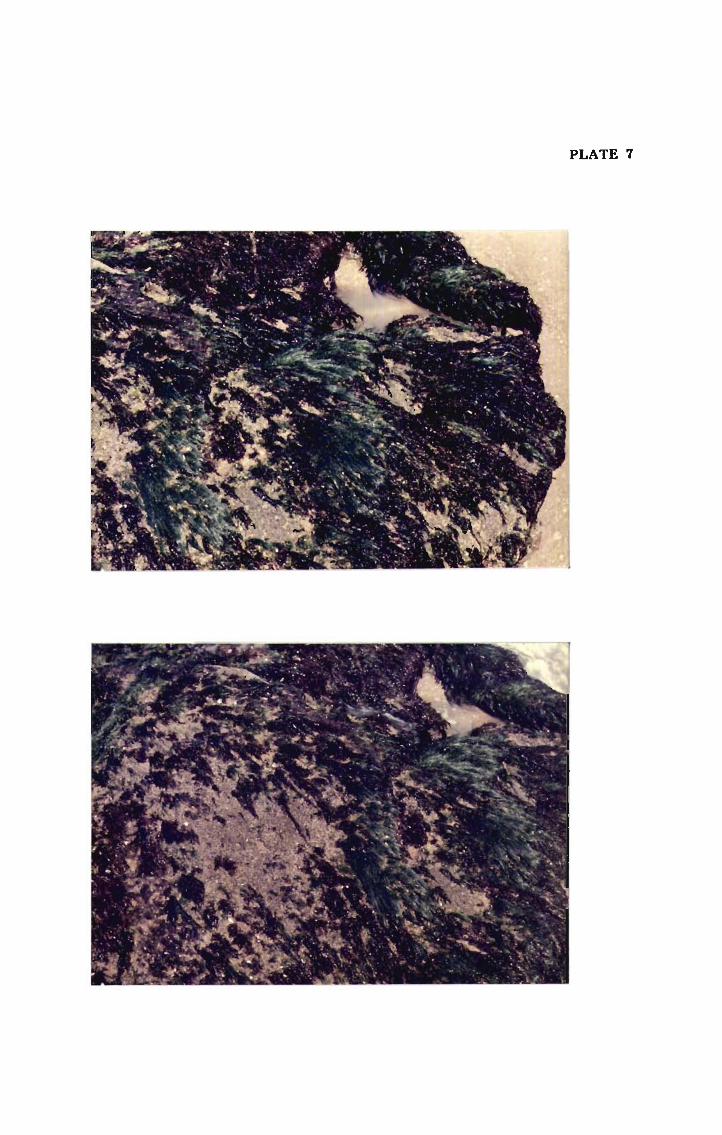
PLATE 7

PLATE 8

Top: Mixed growth of Gigartina acicularis and Ulva lactuca seen

at Elathur. Gracilaria corticata and Centroceras clavulatum may

also be noticed.

Bottom: A different view of the above.

PLATE 8

PLATE 9

Top: Mixed growth of Acanthoghora, Gracilaria and Centroceras

- Thikkotti.

Bottom: A rock completely covered by Centroceras clavulatumat Thikkotti.

PLATIS 3

PLATE 10

Top: Rock dominated by Gracilaria corticata at Elathur. Ulva

fasciata and Gratelougia lithoghila are also seen.

Bottom: A rock completely covered by Caulerga Eeltata — Thikkotti.

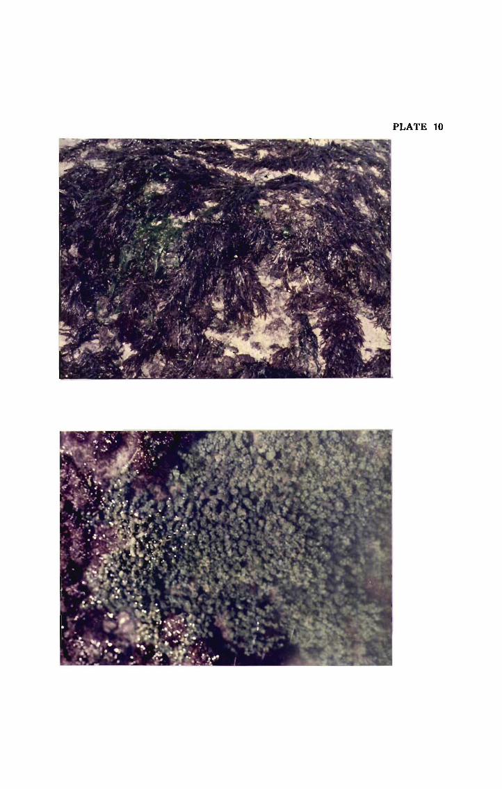
PLATE 10

PLATE 1 1

Top: Gratelougia lithoghila dominated rock at Elathur.

Bottom: A rock covered by Gracilaria corticata - Elathur. Ulva

fasciata and Gratelougia lithoghila can also be seen.

PLATE 1 1

PLATE 12

Top: Artificial dykes of rubble sunken in the sea at Saudi (Fort

Kochi). Chaetomorpha antennina may be seen growing on the

seaward side of the rocks. Centroceras clavulatum is seen growing

on the upper portion of the rocks.

Bottom: A different location of seaweed growth at Saudi.

PLATE 12

PLATE 13

Locations of seaweed growth Saudi.

PLATE 13

PLATE 14

Different views of the seaweed growing areas - Saudi.

PLATE 14

PLATE 15

Mixed growth of seaweeds at Mullur - Ulva fasciata, Caulerpa

peltata, Spyridea filamentosa, Sargassum wightii and Dictyota

bartagresiana.

PLATE 15

,A ,_ ,vhf» , e" = .. “

PLATE 16

Luxuriant growth of species of Sargassum on the seaward sideof a rock - Mullur.

PLATE 16

PLATE 17

Locations of seaweed growth at Mullur showing mixed growth of

Caulerpa peltata, Spyridea filamentosa, Gracilaria corticata and

Sargassum wightii. Association of seaweeds with sea anemone,

bivalves etc. may be noticed, in the background.

PLATE 17

PLATE 18

Some other areas of seaweed growth at Mullur.

PLATE 18

PLATE 19

Flat topped rocks at varying distances from the shore, scattered

in the sea at different depths, showing luxuriant growth of seaweeds

- Mullur.

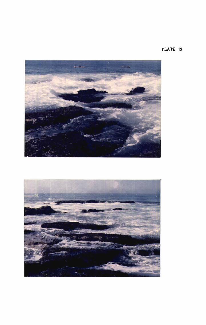
PLATE 19

PLATE 20

Other sites of seaweed growth at Mullur.

PLATE 20-- '!fi$3'-xix»

PLATE 2 1

Different views of seaweed beds at Mullur.

PLATE 21

PLATE 22

View of rocks covered by seaweeds exposed during low tide - Mullur.

PLATE 22

PLATE 23

Top: Chaetomorpha antennina and Ulva lactuca growing on arock at Mullur.

Bottom: Another site of seaweed growth at Mullur.

PLATE 23

PLATE 24

Top: Luxuriant growth of seaweeds on a rock at Mullur close

up view.

Bottom: A big rock protruding into the sea at Mullur. Seaweeds

grow at various levels on the submerged portion of this rock.

PLATE 24

4.8 ENVIRONMENTAL FEATURES OF KERALA COAST

4.8.1 Environmental data recorded at the various stations

Table 33. Environmental data recorded at Mullur

Year Months Temperature Dissolved Salinity Phosphate Nitrate SilicateOxygen

AT SWT ml/1 ppt /ugat/1 /ugat/1 /ugat/1

Feb. 29.00 30.00 3.60 30.00 1.00 0.50 0.20Mar. 31.00 30.00 4.90 35.00 0.90 0.50 0.10Apr. 32.00 31.00 4.60 30.00 1.07 0.60 0.20May 32.00 30.50 5.00 31.00 1.00 1.30 0.15Jun. 30.00 26.00 4.60 34.20 1.08 1.50 0.75

1988 Jul. 27.00 25.00 5.00 34.20 1.08 2.85 1.60Aug. 29.50 27.00 5.00 35.00 0.36 0.90 0.05Sep. 28.00 27.00 4.00 33.20 3.24 2.70 0.06Oct. 28.00 29.00 4.30 35.40 0 1.20 0.07Nov. 33.20 30.00 4.90 33.00 0 2.85 0.05Dec. 26.00 28.00 7.60 33.00 0 0.75 0.05Jan. 30.00 29.00 6.13 33.40 0 0.15 0.20Feb. 35.00 30.00 7.10 34.00 0.72 1.20 0.25Mar. 28.00 28.00 7.70 34.00 1.55 0.60 0.08Apr. 28.00 28.00 3.60 34.70 2.25 0.90 0.17May 27.00 25.00 6.80 32.20 1.00 1.20 0.11Jun. 27.00 26.00 6.90 31.50 1.40 1.30 0.08

1989 Jul. 27.00 23.00 4.00 34.00 1.40 2.00 0.07Aug. 27.00 23.00 4.30 34.00 3.20 0.80 0.17Sept. 29.00 28.00 4.80 32.00 2.80 2.40 0.08Oct. 28.00 27.00 4.90 32.00 0 1.00 0.03Nov. 30.00 30.00 5.00 31.50 0 2.00 0.04Dec. 29.00 28.00 6.50 32.00 0 0.80 0.07

1990 Jan. 30.00 29.00 6.00 32.50 0.90 0.20 0.20Mean 29.19 27.80 5.30 32.99 1.04 1.26 0.20

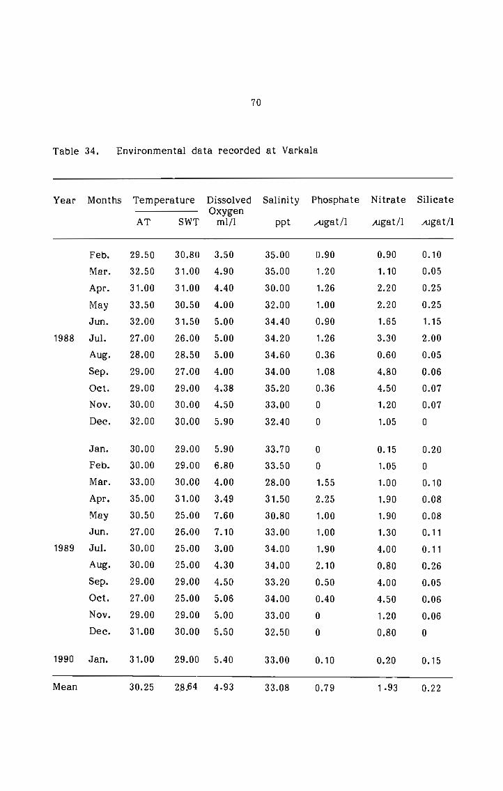
70

Table 34. Environmental data recorded at Varkala

Year Months Temperature Dissolved Salinity Phosphate Nitrate SilicateOxygenAT SWT ml/1 ppt /ugat/1 /ugat/l /ugat/l


1988 Jul. 27.00 26.00 5.00 34.20 1.26 3.30 2.00Aug. 28.00 28.50 5.00 34.60 0.36 0.60 0.05Sep. 29.00 27.00 4.00 34.00 1.08 4.80 0.06Oct. 29.00 29.00 4.38 35.20 0.36 4.50 0.07Nov. 30.00 30.00 4.50 33.00 0 1.20 0.07Dec. 32.00 30.00 5.90 32.40 0 1.05 0Jan. 30.00 29.00 5.90 33.70 0 0.15 0.20Feb. 30.00 29.00 6.80 33.50 0 1.05 0Mar. 33.00 30.00 4.00 28.00 1.55 1.00 0.10Apr. 35.00 31.00 3.49 31.50 2.25 1.90 0.08May 30.50 25.00 7.60 30.80 1.00 1.90 0.08Jun. 27.00 26.00 7.10 33.00 1.00 1.30 0.11

1989 Jul. 30.00 25.00 3.00 34.00 1.90 4.00 0.11Aug. 30.00 25.00 4.30 34.00 2.10 0.80 0.26Sep. 29.00 29.00 4.50 33.20 0.50 4.00 0.05Oct. 27.00 25.00 5.06 34.00 0.40 4.50 0.06Nov. 29.00 29.00 5.00 33.00 0 1.20 0.06Dec. 31.00 30.00 5.50 32.50 0 0.80 0

1990 Jan. 31.00 29.00 5.40 33.00 0.10 0.20 0.15Mean 30.25 28.54 4-93 33.08 0.79 1-93 0.22

71

Table 35. Environmental data recorded at Elathur

Year Months Temperature Dissolved Salinity Phosphate Nitrate SilicateOxygenAT SWT ml/1 ppt ,ugat/1 /ugat/1/ugat/1


1988 Jul. 27.00 28.00 3.50 29.00 1.00 2.00 3.00Aug. 28.00 27.50 5.20 23.00 3.06 3.30 4.90Sep. 30.50 30.00 4.25 29.60 0.72 7.20 0.40Oct. 32.00 30.00 3.40 28.80 2.34 3.00 0.20Nov. 31.00 30.00 4.25 36.60 2.34 3.30 0.14Dec. 31.00 31.00 5.80 33.70 0 1.20 0.10Jan. 25.00 29.00 5.00 33.10 1.08 2.10 0.60Feb. 32.00 31.50 5.46 34.00 0 1.02 0Mar. 31.50 31.00 3.89 27.00 2.25 0.90 0.30Apr. 32.00 31.00 3.30 36.00 2.25 1.80 0.30May 30.00 29.50 5.50 34.00 2.30 2.20 0.10Jun. 27.00 28.00 3.70 27.00 4.60 1.00 0.08

1989 Jul. 23.50 22.50 3.85 21.00 1.00 3.00 0.11Aug. 28.00 29.00 4.25 33.00 1.46 2.90 0.44Sep. 29.00 29.00 3.70 26.20 2.80 6.70 0.35Oct. 30.00 30.00 3.40 29.00 2.20 2.90 0.20Nov. 31.00 29.00 4.50 35.00 2.20 3.00 0.10Dec. 32.00 31.00 5.40 32.00 0 0.90 0

1990 Jan. 26.00 28.00 4.90 32.00 1.20 1.00 0.30Mean 29.50 29.38 4.20 29-83 1.61 2.35 0.78

72

Table 36. Environmental data recorded at Thikkotti

Year Months Temperature Dissolved Salinity Phosphate Nitrate SilicateOxygenAT SWT ml/l ppt /ugat/1 ,ugat/l /ugat/1


1988 Jul. 26.00 25.00 5.60 28.00 1.98 1.05 1.70Aug. 27.00 26.00 4.60 29.00 2.16 4.50 3.90Sep. 28.00 27.00 4.60 30.00 1.80 1.50 0.05Oct. 29.00 27.50 3.60 34.70 3.42 1.20 0.03Nov. 34.00 33.00 5.50 35.50 0.18 4.05 0Dec. 32.00 31.50 7.60 34.60 0 4.80 0.10Jan. 28.00 29.00 6.70 33.00 1.08 1.50 0.20Feb. 33.00 32.00 8.00 35.30 0 3.90 0Mar. 31.50 31.00 4.30 29.30 1.55 0.60 0.10Apr. 28.00 28.00 4.12 31.50 1.55 1.20 0.19May 30.00 28.00 8.00 33.20 1.00 1.50 0.07Jun. 25.00 27.00 7.60 30.80 2.80 5.00 0.04

1989 Jul. 25.00 22.50 3.50 30.60 1.40 1.00 0.17Aug. 27.00 26.00 4.80 32.90 4.40 3.50 0.50Sep. 28.00 28.00 5.86 27.00 1.90 1.30 0.03Oct. 29.00 27.50 4.00 30.00 2.16 1.20 0.01Nov. 32.00 33.00 5.00 33.00 0.20 3.50 0Dec. 32.00 31.50 6.00 33.50 0 4.20 0.10

1990 Jan. 29.00 29.00 5.60 33.00 1.00 1.30 0.30Mean 29.44 29.02 5.19 31.56 2.08 2.74 0.44

73

Table 37. Environmental data recorded at Saudi

Year Months Temperature Dissolved Salinity Phosphate Nitrate Silicate———— OxygenAT SWT ml/1 ppt /ugat/1 /ugat/1 /ugat/1


1988 Jul. 30.00 29.00 5.29 22.00 1.08 1.80 3.70Aug. 31.00 29.50 4.79 21.40 1.08 2.55 0.60Sep. 30.00 29.00 4.47 20.00 2.88 2.40 0.02Oct. 29.00 28.50 4.35 25.00 5.22 3.60 1.75Nov. 30.00 29.50 4.30 34.00 0 0 0Dec. 34.00 30.00 5.59 33.70 0 1.50 0Jan. 30.00 32.00 5.62 33.00 1.54 1.50 0.45Feb. 32.00 31.00 6.40 34.40 0 2.70 0.05Mar. 33.00 30.50 4.12 30.00 2.25 0 0.19Apr. 32.00 31.00 3.49 32.50 3.80 6.50 1.20May 33.30 31.00 8.00 26.00 2.90 0.15 0.06Jun. 30.00 29.00 5.00 27.00 2.00 6.00 0.44

1989 Jul. 28.00 27.00 3.87 18.00 1.00 1.30 1.-75Aug. 29.00 28.00 3.80 31.70 1.90 2.00 0.33Sep. 33.00 31.00 4.79 17.00 1.90 1.90 0.03Oct. 29.00 28.00 4.70 28.00 3.25 3.00 1.50Nov. 30.00 30.00 4.50 32.00 0 0 0Dec. 33.00 31.00 5.00 33.00 0 1.30 0

1990 Jan. 31.00 30.00 4.80 32.00 1.30 1.20 0.35

Mean 30.38 29.79 4.62 28.38 1.79 2.80 0,84

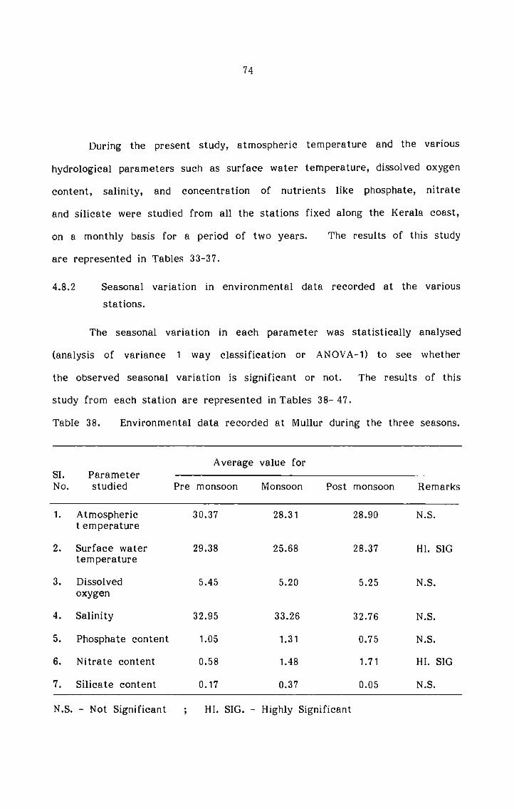
74

During the present study, atmospheric temperature and the various

hydrological parameters such as surface water temperature, dissolved oxygen

content, salinity, and concentration of nutrients like phosphate, nitrate

and silicate were studied from all the stations fixed along the Kerala coast,

on a monthly basis for a period of two years. The results of this study

are represented in Tables 33-37.

4.8.2 Seasonal variation in environmental data recorded at the variousstations.

The seasonal variation in each parameter was statistically analysed

(analysis of variance 1 way classification or ANOVA—1) to see whether

the observed seasonal variation is significant or not. The results of this

study from each station are represented in Tables 38- 47.

Table 38. Environmental data recorded at Mullur during the three seasons.

Average value forS1. Parameter No. studied Pre monsoon Monsoon Post monsoon Remarks

1. Atmospheric 30.37 28.31 28.90 N.S.temperature

2. Surface water 29.38 25.68 28.37 HI. SIGtemperature

3. Dissolved 5.45 5.20 5.25 N.S.oxygen

4. Salinity 32.95 33.26 32.76 N.S.5. Phosphate content 1.05 1.31 0.75 N.S.6. Nitrate content 0.58 1.48 1.71 HI. SIG7. Silicate content 0.17 0.37 0.05 N.S.N.S. - Not Significant ; HI. SIG. — Highly Significant

75

Table 39. Environmental data recorded at Varkala during the three seasons.

Average value for

EC’). Psatlfijrinezter Pre monsoon Monsoon Post monsoon Remarks

1. Atmospherictemperature 31.50 29.75 29.50 N.S.2. Surface watertemperature 30.10 27.19 28.63 N.S.3. Dissolved oxygencontent 4.79 5.13 4.86 N.S.4. Salinity 32.46 33. 38 33.40 N.S.5. Phosphate content 0.90 1.19 0.29 N.S.6. Nitrate content 1.06 1.97 2.76 N.S.7. Silicate content 0.12 0.50 0.05 N.S.N.S. - Not Significant

Table 40. Environmental data recorded at Elathur during the three seasons.

Average value forS1. Parameter RemarksNo. studied Pre monsoon Monsoon Post monsoon

1. Atmospherictemperature 30.00 27.69 30.80 N.S.2. Surface watertemperature 30.38 27.75 30.00 HI. SIG.3. Dissolved oxygencontent 4.14 4.13 4.34 N.S.4. Salinity 31.39 26.75 31.36 N.S.5. Phosphate content 1.13 2.13 1.58 N.S.6. Nitrate content 1.29 2.24 3.52 N.S.7. Silicate content 0.52 1.64 0.19 N.S.N.S. — Not Significant ; HI. SIG. - Highly Significant

76

Table 41. Environmental data recorded at ’l‘hikkotti during the three seasons.

Average value forS1. Parameter RemarksNo’ Studled Pre monsoon Monsoon Post monsoon


2. Surface water 30. 50 26.69 29.87 HLSIG.temperature

3. Dissolved oxygen 5.19 5.14 5.27 N.S.content

4. Salinity 31.39 31.00 32.28 N.S.5. Phosphate content 2.18 2.84 1.21 N.S.6. Nitrate content 2.41 3.09 2.72 N.S.7. Silicate content 0.24 1.03 0.04 N.S.N.S. - Not Significant ; HI. SIG. - Highly Significant

Table 42. Environmental data recorded at Saudi during the three seasons

Average value forS1. Parameter RemarksNo‘ studled Pre monsoon Monsoon Post monsoon


2. Surface water 31.00 28.75 29.63 HI. SIGtemperature

3. Dissolved oxygen 4.32 4.84 4.71 N.Scontent

4. Salinity 32.11 25.18 27.84 N.S.5. Phosphate content 1.76 1.97 1.66 N.S.6. Nitrate content 3.83 2.87 1.71 N.S.7. Silicate content 0.55 1.55 0.41 N.S.N.S. - Not Significant ; HI. SIG. - Highly Significant

77

Surface water temperature showed a significant variation between

seasons in all stations, except Varkala. Refer ANOVA (analysis of variance)

Tables below:

Table 43. Variation in surface water temperature at Mullur between seasons

SOURCE D.F. SUM.SQR MEAN. SQR F-VAL RAMARKS

TREAT 2 58.188 29.094 10.49 HI. SIG(1%)ERROR 21 58. 219 2.772

MEAN COMPARISONS REMARKST 1 - T 2 SIGT 1 — T 3 N.S.T 2 - ’I‘ 3 SIGSIG — Significant ; N.S. - Not Significant ; HI. SIG - Highly SignificantT 1 - Pre monsoon ; T 2 — Monsoon ; T 3 - Post monsoon

Table 44. Variation in surface water temperature at Elathur between seasons

SOURCE D.F. SU1VI.SQR MEAN. SQR F-VAL REMARKS

TREAT 2 32.25 16.125 6.79 HI.SIG(1%)ERROR 21 49.875 2.375MEAN COMPARISONS REMARKST 1 — T 2 SIGT 1 - T 3 N.S.T 2 - T 3 SIGSIG - Significant ; N.S. — Not Significant ; HI. SIG - Highly SignificantT 1 - Pre monsoon ; T 2 - Monsoon ; T 3 - Post monsoon

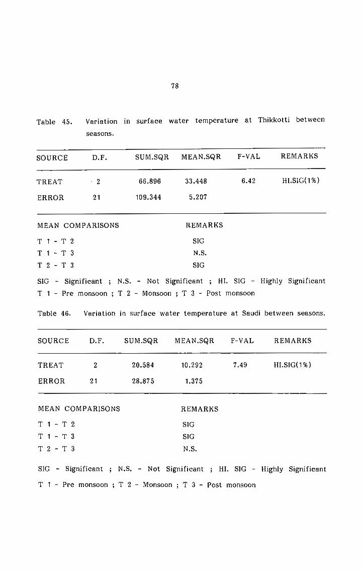
78

Table 45. Variation in surface water temperature at Thikkotti betweenseasons.

SOURCE D.F. SUM.SQR MEAN.SQR F-VAL REMARKS

TREAT - 2 66.896 33.448 6.42 HI.SIG(1%)ERROR 21 109.344 5.207

MEAN COMPARISONS REMARKST 1 - T 2 SIGT 1 - T 3 N.S.T 2 - T 3 SIGSIG - Significant ; N.S. - Not Significant ; HI. SIG — Highly SignificantT 1 — Pre monsoon ; T 2 - Monsoon ; T 3 — Post monsoon

Table 46. Variation in surface water temperature at Saudi between seasons.


TREAT 2 20.584 10.292 7.49 HI.SIG(1%)ERROR 21 28.875 1.375

MEAN COMPARISONS REMARKST 1 - T 2 SIGT 1 - T 3 SIGT 2 — T 3 N.S.SIG — Significant ; N.S. - Not Significant ; HI. SIG - Highly Significant

T 1 - Pre monsoon ; T 2 - Monsoon ; T 3 - Post monsoon

79

At Mullur, nitrate content also varied significantly between seasons

(Table 47).

Table 47. Variation in nitrate content at Mullur between seasons.



MEAN COMPARISONS REMARKST 1 - T 2 SIGT 1 - T 3 SIGT 2 - T 3 N.S.SIG - Significant ; N.S. - Not Significant ; HI. SIG — Highly SignificantT 1 Pre monsoon ; T 2 — Monsoon ; T 3 — Post monsoon

No other parameter showed significant seasonal variation in anyof the stations studied.

4.8.3. Comparison of environmental data from different stations.

Table 48. Comparison of environmental data from different stations

Average value atSl. ParameterNo. Studied Mullur Varkala Thikkotti Elathur Saudi1. Atmospherictemperature 29.19 30.25 29.44 29.50 30.882. Surface water

temperature 27.80 28.64 29.02 29.38 29.793. Dissolved oxygen 5.30 4.93 5.19 4.20 4.624. Salinity 32.99 33.08 31.56 29.83 28.385. Phosphate content 1.04 0.79 2.08 1.61 1.796. Nitrate content 1.26 1.93 2.74 2.35 2.807. Silicate content 0.20 0.22 0.44 0.78 0.84

80

Statistical analysis (analysis of variance 2 way classification or

ANOVA-II) was done to see whether the observed variation in each factor,

between stations was significant or not.

(1)

The results are given below:

Atmospheric temperature did not vary significantly between stations.

Among the stations the lowest mean atmospheric temperature was

recorded at Mullur (29.19°C) and the highest at Saudi (3U.875°C).

(2) Surface water temperature varied significantly between stations

(Table 49).

Table 49. Variation in surface water temperature between stations.


TREAT 4 6.849 1.712 6.62 SIG (5%)REPLIC 2 24.417 12.208 47.18 HI.SIG(1%)ERROR 8 2. 070 0.259

TREATMENT MEAN COMPARISONS REMARKST 1 - T 2 N.S.T 1 - T 3 SIGT 1 - T 4 SIGT 1 - T 5 SIGT 2 - T 3 N.S.T 2 — T 4 N.S.T 2 - T 5 SIGT 3 - T 4 N.S.T 3 - T 5 N.S.T 4 - T 5 NS,

81

Table 49 (Contd...)

REPLICATION MEAN COMPARISONS REMARKSR1 - R2 SIGR1 - R3 SIGR2 - R3 SIGN.S. — Not Significant ; SIG — Significant ; HI.SIG — Highly Significant

T1 - Mullur ; T2 - Varkala ; T3 - Thikkotti ; T4 — Elathur ; T5 — Saudi

R1 - Pre monsoon ; R2 - Monsoon ; R3 — Post monsoon

Mullur recorded the lowest mean surface water temperature (27.80°C) and

Saudi the highest (29.79°C).

(3) Dissolved oxygen content varied significantly between stations(Table 50).

Table 50. Variation in dissolved oxygen content between stations.


TREAT 4 2.406 0.602 19.5 HI.SIG(1%)REPLIC 2 0.036 0.018 0.59 N.S.ERROR 8 0.247 0.031

TREATMENT MEAN COMPARISONS REMARKST 1 - T 2 SIGT 1 - T 3 N.S.T 1 - T 4 SIGT 1 - T 5 SIGT 2 - T 3 N.S.

82

Table 50 (Contd....)

TREATMENT MEAN COMPARISONS REMARKST 2 - T 4 SIGT 2 - T 5 N.S.T 3 - T 4 SIGT 3 - T 5 SIGT 4 - T 5 SIGN.S. - Not Significant ; SIG - Significant ; HI.SIG - Highly SignificantT1 - Mullur ; T2 - Varkala ; T3 - Thikkotti ; T4 - Elathur ; T5 - SaudiR1 - Pre monsoon ; R2 — Monsoon ; R3 — Post monsoon

Elathur recorded the lowest mean dissolved oxygen content (4.2 ml/1) and

Mullur the highest (5.3 ml/1).

(4) Salinity did not vary significantly between stations. The lowest

mean salinity was recorded at Saudi (28.38 ppt) and the highest

at Varkala (33.08 ppt).

(5) Phosphate content varied significantly between stations (Table 51).

Table 51. Variation in phosphate content between stations.

SOURCE D.F. SUM.SQR MEAN.SQR F—VAL REMARKS

TREAT 4 3.402 0.350 7.68 I-II.SIG(1%)REPLIC 2 1.594 0.797 7.20 SIG (5%)ERROR 3 0.886 0.111TREATMENT MEAN COMPARISONS REMARKST 1 - T 2 N.S.T 1 — T 3 SIGT1-T4 N.S.

83

Table 51 (Contd...)

TREATMENT MEAN COMPARISONS REMARKST 1 - T 5 SIGT 2 - T 3 SIGT 2 - T 4 SIGT 2 - T 5 SIGT 3 - T 4 N.S.T 3 - T 5 N.S.T 4 - T 5 N.S.REPLICATION MEAN COMPARISONS REMARKSR1 - R2 N.S.R1 - R3 N.S.R2 - R3 SIGN.S. - Not Significant ; SIG - Significant ; HI.S1G - Highly Significant

T1 - Mullur ; T2 - Varkala ; T3 - Thikkotti ; T4 — Elathur ; T5 - Saudi

R1 - Pre monsoon ; R2 — Monsoon ; R3 - Post monsoon

Varkala recorded the lowest mean phosphate content (0.79 /ugat/1) and

Thikkotti the highest (2.08»ugat/1).

(6) Nitrate content did not vary significantly between stations. Lowest

mean nitrate content was recorded at Mullur (1.26 xugat/1) and the

highest at Saudi (2.8 /ugat/l).

(7) Silicate content varied significantly between stations (Table 52).

84

Table 52. Variation in silicate content between stations


TREAT 4 1.088 0.272 4.21 SIG (5%)REPLIC 2 2.108 1.054 16.31 Hl.SIG(1%)ERROR 8 0.517 0.065TREATMENT MEAN COMPARISONS REMARKST 1 - T 2 N.S.T 1 - T 3 N.S.T 1 - T 4 SIGT 1 - T 5 SIGT 2 — T 3 N.S.T 2 - T 4 SIGT 2 - T 5 SIGT 3 - T 4 N.S.T 3 - T 5 N.S.T 4 - T 5 N.S.REPLICATION MEAN COMPARISONS REMARKSR1 - R2 SIGR1 - R3 N.S.R2 - R3 SIGN.S - Not Significant ; SIG — Significant ; HI.SIG — Highly Significant

T1 - Mullur ; T2 - Varkala ; T3 — Thikkotti ; T4 - Elathur ; T5 — Saudi

R1 — Pre monsoon ; R2 - Monsoon ; R3 - Post monsoon

85

Lowest mean silicate content was recorded at Mullur (0.2 /ugat/1) and the

highest at Saudi (0.84'zugat/1).

4.8.4 Correlation between environmental factors observed at the variousstations.

Statistical analysis (Correlation matrix) revealed some relationships

between the various environmental factors studied at each station. These

are given below:

At Mullur,

A positive correlation was observed between atmospheric and surface water

temperature and the 'r' value was 0.7.

A negative correlation was observed between surface water temperature

and phosphate content with an 'r' value of -0.413.

At Varkala,


temperature with an 'r' value of 0.63.

A negative correlation was observed between atmospheric temperature and

salinity with an 'r' value of -0.482.

A negative correlation was observed between dissolved oxygen and phosphate

content with an 'r' value -0.479.

At Elathur,



86

A positive correlation was observed between atmospheric temperature and

salinity with an ‘r‘ value of 0.428.

A positive correlation was observed between surface water temperature

and salinity with an 'r' value of 0.571.

A negative correlation was observed between dissolved oxygen content and

phosphate content with an 'r' value of -0.396.

A negative correlation was observed between salinity and silicate content

with an 'r' value of -0.510.

At Thikkotti,

A positive correlation was observed between atmospheric temperature and

surface water temperature with an 'r' value of 0.911.

A negative correlation was observed between dissolved oxygen and phosphate

content with an 'r' value of -0.586.

At Saudi,



A positive correlation was observed between surface water temperature

and salinity with an 'r' value of 0.515.

A negative correlation was observed between nitrate content and dissolved

oxygen content with an 'r' value of -0.407.

Silicate content was found to have a negative correlation with atmospheric

temperature, surface water temperature and salinity with 'r' values -0.458,

-0.520 and -0.388 respectively.

4.9 CORRELATION BETWEEN ENVIRONMENTAL FACTORS ANDTHE DENSITY OF SEAWEEDS

Correlation between environmental factors studied and the density

of selected species of seaweeds, from each station was studied statistically

(Correlation matrix). Results of this study are represented in Table 53.

Table 53. Correlation between environmental factors and the densityof seaweeds

Names of seaweeds Environmental Type of Co-efficient Station inParameters correlation of correlation whichshowing observed 'r‘ value correlationcorrelation was observedwith density

Ulva fasciata Atmospherictemperature Negative -0.552 VarkalaSurface watertemperature Negative -0.472 VarkalaNitrate content Positive 0.415 VarkalaDissolvedoxygen content Positive 0.567 ElathurPhosphatecontent Negative -0.502 ElathurSilicatecontent Positive 0.444 Mullur

2. lactuca Atmospherictemperature Negative -0.411 VarkalaDissolvedoxygen content Positive 0.438 ElathurSilicatecontent Positive 0.680 Varkala

Table 53 (Contd...)

Names of seaweeds Environmental Type of Co-efficient Station inparameters correlation of correlation whichshowing observed 'r‘ value correlationcorrelation was observedwith density

Bryopsis plumosa Atmospherictemperature Positive 0.461 MullurChaetomorpha Silicateantennina content Positive 0.737 ThikkottiCladophora Dissolvedglomerata oxygen content Positive 0.390 Thikkotti

Phosphate Negative -0.467 Thikkotticontent

__C_aulerp_a Salinity Positive 0.430 Thikkotti_sertularioides

Enteromorpha Salinity Negative -0.592 Saudicomgressa silicate Positive’ 0.50 Saudicontent

Chnoospora Phosphate Positive 0.390 Mullurminima contentNitratecontent Positive 0.418 Mullur

Padina Atmospheric Positive 0.399 Mullurgymnospora temperature

Surface watertemperature Positive 0.454 Mullur

Gracilaria Silicate Positive 0.399 Mullurcorticata contentSpyridea Nitratefilamentosa content Negative -0.470 Mullur

Table 53 (Contd...)

89

Names of seaweeds Environmental Types of Co-efficient Station inparameters correlation of correlation whichshowing observed 'r' value correlationcorrelation was observedwith density

Porphyra ' Atmospherick anyakumariensis temperature Negative -0.434 Mullur

Surface watertemperature Negative -0.669 Mullur

Gratelgupia Atmospheric Positive 0.463 Varkalalithophila temperature

Dissolvedoxygencontent Positive 0.478 MullurDissolvedoxygencontent Positive 0.436 VarkalaNitratecontent Negative -0.499 Varkala

Q. filicina Nitratecontent Positive 0.452 ElathurGelidiopsis Salinity Positive 0.601 Elathurvariabilis

Gigartina Dissolved Positive 0.440 Thikkottiacicularis oxygencontent

Centroceras Phosphate Negative -0.557 Varkalaclavulatum contentNitrate Negative -0.428 Varkalacontent

90

It is clear from Table 53 that the density of each species of seaweed

studied, was showing a correlation of some kind with one or more of the

environmental factors monitored. Therefore it may be said that each species

of seaweed requires a specific combination of environmental factors for

its biomass production.

5. BIOCHEMICAL OBSERVATIONS

5.1 BIOCHEMICAL COMPOSITION OF SEAWEEDS FROM VARIOUSSTATIONS ALONG KERALA COAST

5.1.1 Biochemical composition of some seaweeds from Mullur (Tables54-57 6( Figs. 4-12)

At Mullur, for green algae

Highest protein content of 16.4% was observed in Enteromorpfla compressa

(July 1989) and the lowest of 1.4% in Ella lactuca (March 1988) and (March

1989).

Caulerpa peltata (February 1989) recorded the highest carbohydrate content

of 75% and Chaetomorpha antennina (July 1989) the lowest of 8.75%.

Bryopsis plumosa (February 1989) and Caulerpa peltata (January 1989)

recorded the highest lipid content of 6.1% and Chaetomorpha antennina

(July 1989) the lowest of 0.9%.

At Mullur, for brown algae

Pajwia gymnospora (May 1989) recorded the highest protein content of

16.4% and the same alga in February 1988 recorded the lowest of 2.8%.

Sargassum wightii (February 1989) recorded the highest carbohydrate content

of 16.75% and Padina gymnospora (February 1988) recorded the lowestof 3.5%.

Padina gymnospora (December 1989) recorded the highest lipid content

of 8.75% and Sargassum wightii (May 1988) recorded the lowest of 1%.

92

At Mullur, for red algae

Porphyra kanyakumariensis (June 1989) recorded the highest protein content

of 19.6% and Gratelougia lithoghila (March 1989) the lowest of 2.3%.

Gracilaria corticata (April 1989) recorded the highest carbohydrate content

of 37.5% and Hygnea valentiae (March 1989) the lowest of 6%.

Gracilaria foliifera (March 1988) recorded the highest lipid content of 5.5%

and Centroceras clavulatum (November 1988) the lowest of 0.5%.

93

5.2 8.8. 8.8 8.. 3.8 5.2 mo<mm><

8.2 8.8 8.8 2.. 8.8 8.8 as. 82

8.8 8.8 8.8 8.8 8.: 8.2 .358.8 8.8 8.8 8.8 8.: 8.2 .328.8 8.8. 8.8 8.8 8.8 8.2 .308.8 8.8 8.8 8.8 8.2 8.2 .888.2 8.8 8.8 8.. 8.8 8.2 .928.2 3.8 8.8 8.8 8.2 8.2 43.

8.8 8.: 3.8 8.8 8.2 8.: .5... 82

8.2 8.8 8.3 8.8 8.8 8.2 8:8.8 8.8. 2.8 8.8 8:8 2... .238.2 8.3; 8.2 8.. 8.8 8.8 .828.2 8.8 8.8 2.. 8.8 8.8 .258.2 8.8 8.8, 2.. 8.8 8.8 .52.8.8 8.: 8.8 8.8 8.2 8.2 .328.2 8.82 8.8 8.2 8.8 8.: .508.8 84.2 8.8 8.8 8.8 8.2 .888.2 8.2: 8.8 8.. 8.8 88 .m=<

8.2 8.8. 8.2 8.. 8.8 8.2 .5. 82

8.2 8.22 8.8 8.8 8.8 8.8 .5...8.2 8.2; 8.8 8.8 8.8 8.8 .28.

3.2 8.2. 8.8 2.8 8.8 8.2 .88 8885 alzm ._was 8968880 530.5 Ea: 82EEo2wo 5895 838:8 .33 82 2. 282 52

mo v3w> o_.:._o_wO mo mmwucmopmm no 5:02 .5

._:::_>_ E0...“ mam? cwmzm mEom we :O_u_mOQEOU _ao_Ewcoo_m_ :vm @369

94

ammm._mEoo

8;; 8.2. 8.8 8.; 8.2 8.2 .3;. 82 3% .8

8.8 8.2; 8.8 8.8 2.8 2.2 mo<mm><

8.2 8.2; 8.8 8.; 8.8 8.; 8;. 82

8.8 8.8; 8.8 2.5 8.8 8.2 .898.8 8.8; 2.8 8.8 8.8 8.2 .828.8 8.8 2.8 8.8. 8.8 8.2 .308.2 2.2.; 8.8 8.8 8.8 8.2 .982.2 8.8; 8.8 8; 8.8 8.2 .m=<8.8 8.8; 2.8 8.; 8.8 8.;; .;=;.8.8 8.8; 8.8 21. 8.8 8.2 828.2 8.2; 8.; 8.; 8.8 2.; ..as_

8.2 8.8; 8.8 2.; 8.8 8.8 .29; 82

8.8 8.8; 8.8 8.2.. 8.8 8.2 .358.8 2.8; 8;; 8.8 8.2.. 8.2 .828.8 8.8; 2.8 8.8 8.8 8.2 8m8.2 8.8; 8.8 2.; 8.8 8.2 .m:<8.2 8.8 8;; 8.; 8.8 8.8 .328.2. 3.8 8; 8.8 8.2 8.; .82

8.8 8.8; 5.8 8;. 8.8 8.8 59; 82 moflofld 8

E9: 3w._EEoa_._aO E3o._m UB5 m;w.6.Eon.EO E3o.E

cofiomzoo So» mm? .;o 0EwZ .oz.;o w_.:w> UC_._O_wO .;o mm3:mo.6m .;o £u:O_>_ AmA.:3:oOv 8 23¢?

Zflmv nm.:m 9.; m—.m co.m~. 8.2 dam

38.88 8.82 88.; 2.8 8.88 2...; .88 82

8.28 884...... 8.88 8.8 8.8 8.2 .88.8.8 8.8.2 8.8 8.8 8.8 8.2 .328.8 8.8: 8...? 8.8 8.8 8.2 .808.8 88.82 2.8 8.8 8.88 8.2 .88

325 88.28 83:. 8.8 8.88 8.2 .83.. mg

8.2. 88...: 8.88 8.8 2.88 2.2 as. 82 8.5380 .8

woflzm

8.88 88.88 8.8 2.8 8.8 2.8_ .88 82 wfimwfl .8

% 8.8 8.8.8 8.8 8.8 8.2 8.2 mo<mm><8.28 2.2. 8.8 8.8 ..:..m 8.2 .882.8 8.8 8.8 2.8 88.2 8.2 .83..2.8 8.8 8.2. 8.8 88.8 8.8 .3888.88 88.88 8.: 88.8 8.2 8.2 .:3.

8.8 8.88 «~48 8.8 88.2 8.8 .88 82

2.88 3.3 8.8 88.8 88.8 8.2 .83.8.8 88.88 88.8 8.8 8.2 8.8 .88

m:E:3:m

88.88 2.8 8.3. 88.8 8.2 2.8 82 882 § 4.

U_Q_..— 3m._PEon._mO E3o.E U_Q_1— 3w._EEon..mO C_@uOLnm

CO.50w:OU .:8m% 90 mE.®Z .OZQ0 m3w> O_.:LO.—dO 90 mmwucmopwm .«O £u_.._O—>_ JmA...E:o9 _.8 288.8

96

8.8 822 5.8 8.8 3.8 8.2 mo<mm><

8.8 8.22 858 36 8.8 8.2 .52. 82

8.2. 8.82 8.8 83. 8.8 8.2 .258.2 8.3. 8.8 8; 8.8 8.2 .828.8 8.82 3.2. 2.8 8.8 8.2 .808.8 8.82 8.8 2.8 8.8 8.: .888.8 8.2. 8.8 8:8 3.8 8.2 .m=<8.8 8.3 8.2. 8.8 8.2 8.8 ._2.8.8 84.2 2.8 82. 8.8 8.8 as.8.8 8.2: 8.8 3.8 8.8 8.8 $2

8.8 8.82 8.8 8+ 8.8 2.8 .a< misflom8.8 8:28 8.8 8._. 8.8 8.8 .82 82 mag

U_Q_J .3m.6>con..m0 530.5 3m._PEon._wO C_0uO._&

cosowsoo .5»; am? mo QEGZ .OZ..o w:_w> oC_._o_mO ._o wmwacoohwm ..o 5:02 .8A:.U..:oOv 8 22:.

mam., \ , \ , xfi M

& . \ , \D bx / \

3.... <|i4 , \ vx /Qx / \

2o.uEo..:.u OIIO ,, \l\ xxx

.._2...:._ TC mu‘

V9“. m:._.S_2 20mm §3.um.\k V343“.0 zoEmon_s_oo ._<o_2m:oo_m Z_ zo:<_m<>

.2»

39v1N3oa3cT

OON

ION

O['0

ID[0

En:

araza2o._§..3.ou On I IO

1

InN O10c‘: o|'0 N39ViN33H3d

52¢... I

m3.52 20m.... VGDKQVQ 3.33no zoEmoa_2oo ._<o_2mzoo_m z_ zo;<_m<>

6F0

Omm. mmm.

mzpzoz

5 o z o m 4 .. a 2 < .. L a o 2 “V m < . 3 2 < 2 u

xyvuqzar. . . xv. .nr;$us.

¢ ¢ 4 4.4.4 4.1.4 . n

-o_Ln.N -8\ / -n~

xlvi Qb, Nax ,0 w\ . nmo//AX — 1 3/ % , .o¢m/ _ J 4m¢w3 _ . .on3

, . g .nn, _ .ow

, _ V

.._._._<.I._Q , _ //O .32u.E£on.uo On|.O / _ Low.__2.:.. I & Ln»

m.o¢

m:._.:._2 .201... 335mm VQQMQDVU.._o zoEmoas_oo ._<o__2m_..oo_m z_ zo:<E<>

79

w:m_mm._N5.:B

8.8 8.2. 8.2 8.8 8.: S..m .82 82 92% .8

8.2. 2.2. 8.8 21. 8.2 8.: mo<mm><8.8 8.2. 2.8 8.8 8.2 8.: 5oz8.8 8.2. 3.8 8.8 8.2 8.2 .30

8.8 8.8 8.8 8.... $4. 8.: dmm8.8 8.8 8.8 8.8 8; 8.: 83..8.2 8.2. 9.2. 8.8 8.2 8.: .3.8.2. 8.; 2.8 8:. 2.8 8.2 .828.8 8.2. 8.8 8... 8.: 8.: .8m

8.8 8.2. 3.8 23. 8.: 8.2 .58 82

8.8 8.:. 8.8 8.8 8.2 8.: .828.2. 8.2. 8.8 8.2. 8.: 8.2 .608.2. 8.2. 8.8 8.2. 8.: 2...: .888.8 8.2. 8.8 8.8 8.2 8.8 83..

8.8 8.2. 8.8 8.8 8.2 8.... .3. _mmm_|__=|

8.8 8.8 8.2. 8.: 8.2 8.8 .8”: 82 m.§mo4_M .:

was 8EPEo€ao E3o.E 2%. BEEEo€ao E8o.&

:o:om:oo ._mm> mm? mo wEmz 62..o w:_w> OCCOHMO ..o wmficmflwm mo £u:O_>_ Am

._::=_>_ F_o.C mmm_a C395 .......EOm mo :O_u_mOQEOO _ao_Em:oo_m .mm 22$?

98

8.2 8.3. 8.8 8; 2...: 88 as.8.8 8.8 8.8 8.. 8...“ 8.8 828.8 8.; 8.8 .88 8.2 8,.“ .238.8 8.8 8.8 8.8 8.2 8.8 .52

3.: 8.8 8.8 22 8.2 8.» 58 82 ....8.8 8.8 8.8 ...3. 8.: 8.2 .82 82 8:aEo:£E8.I ._.

8.8 8.8 5.8 8.8 N; 88 mo<mm><

8.8 8:; 8.8 8.... 8.2 8.: .52. 89

8.8 3.8 8.8 88 8.8 8.8 .898.8 5.8 8.8 8;. $6 8.8 828...: 8.8 8.8 8; 8.8 8... .828.8 8.; 8.8 83. 8.2 8.2 5.5

8.8 8.2. 8.8 84.. 8.8 88. .52. 82

8.8 8.8 8.8 8.8 8.8 8.» .%.m8.8 8.8 8.8 2:. 88 :3. 828.8 8.8 8.8 8.... 8.... 8+ ..a<

8.2 8.8 8.: 8; 2:. E.” .82 §.mmm.Ham

8.8 8.: 8.2 8...“ 84.. 8.8 5% 82 2.68 .8

2.5 m::EE8.=_..o 530.5 2.3 32938.50 539$

cofiomzoo LNOW ww~< go mEmz .02mo w:_m> OC_._O_mO mo wmmucmohmm mo £u:O_>_ AmA...E:o8 8. 235

99

$.§ 3.3 5.3 $2 3.2 $5 mo<mm><

8.3 3.3 3.3. 8.... 8.: 8.3 .52. 82

3.2. 3.3 3.5 8.... 8.8 8.2 .253.2 3.3 3.2. cm; 8.5 8.3 .>oz3.: 3.; 3.3 $2 2...: omzm .303.3 3.3 33:. 34” co.» 8.? saw2.: 3.3.. 8.3 3.” was 8.9 .m:<3.9 8.2 3.2. 3; 2; S5 43.8.8 3.3 2.3 S; S.» 85 .5...N93 8.: «N23. 23 23 33 >223.9., 3.3 5.3 find mg 36 ..a<3.2 $2 2.: £3 :3 one ..::>_8.: 3.3 3.3 2:. 3.2 as 58

3:3 3.3 E23. 36 8.2 3.2 £3. 82

3.3 2.3. 3.3. 85 Sf 8.2 .808.3 3.3 3.5. 3... 3.: 3.? .>oz2.3 3.2. 3.3 8.”. 8.: 3.3 .802.3 3.2 8.3 85 85 8.5 damom.mm 3% 2.3 om.m 8.9 23 .m:<

3.2 3.2.. 8.2. Ba 85 22 .3. $2 flwmma

E94 3w.6>:on.EO E3o._n_ E94 3w..EEon..wO E3o.E

cofiomzoo Sm». $2 mo wEmz 62mo m2m> o_.:..o_w0 mo mmwucwogwm mo 5:02 .5AEUEOOV mm 298.

mum.

2:...

3.... 4!|.L4o.o3»..on.oo O|.l.IO

£20; I

m=._.jD2 _2om.._ $§<$ v.k0Qm.Q0>_\IUno zoEmo¢2oo ._<o_sa:oo_m Z. zo:<_m<>

01.0_¢

I0 ON. N39V.LN33H3d

ON‘)

mun.

mzpzoz

..._

00$ .

102

— _

2.. __ 4|.I.L4w.EuEo£ou OI IOc_2o:. I

m .5

$3.52 zom... _\..<ooa§<§G 353$.._o zoEmon_2oo ..<o_2mxoo_m z_ zo_»<_m<>

4O

1L0.3 <3(NI CV

39VLN33H3d

1

Off)

®mm_ mflw.

mxpzoz

.._

7 Q

33. driid£o.v».._o€oo OI I I0..__o.oE I

13.332 .22.... E13: ssmmwutwm.._O zo_:mon_2oo ._<o_2m:oo_m z_ zo_.::m<>

0IDan ON N39V.LN33H3d

Orf)

100

23: 3.3 3.3. 8.~ 8.2 8.3 .892.2 3.3 5.5 £2 8.3 3.2 .>oZ8.2 2.3 3.3 22 2.3 8.2 .m:<

8.5 3.: 3.8 23 85 :3 ..::>_ |:|IwmE:m_m>

8.2 3.3. 8.2. S.« 3.3 S; 58.. $2 macaw: 4

22: Sam vo.mN :3 8.2 23 mo<mm><22: no.2. 8.2 8.. 8.: 84.. ..E<

5.3 Be? 8.? awn 8.3.. SE ..::>_ 32

5.2 3.3 2.2.. £2 8.2 85 .>oZ £2 SE95: .m

9:023

3.3 8.2: 22$ omé. Sam 8.? .>oZ £2 m_m:o_3w..0 .~

wmdm mw.mm 3.2: $3 mmam 3.2 mo<mm><8.2 5.2. 8.8 35 E23 8.: .m:<3.2 8.3 3.2: 25 8.8 8.2 43.

2.2 8.3 3.6: 22 3.5 8.2 ._.=:.. $2 m_m:mEmE:xw cmx

3.2 3.92 232 Sam coda O3: 43. $9 E§m..om .—

E94 w:...._EEon._mO 5395 E94 wuwgvzconpmo 530.5

cozowzoo .63» mm? .3 oEwz .ozgo w3m> 2.2030 ..o wmwucwohwm ._o 5:02 ._m

._:::_>_ E95 mwmfi cm: wEom mo :o_:moaEoo _mo_EmEoo_m dm mfiwe

101

8.8 8.8 8.8 2.8 8.2 8.8 dom8.8 8.8 8.2. 8.8 8.: 8.8 .83;8.8 8.8 8.2. 8.8 8.2 8.8 .3.8.2 8.8 8.8 2.; 8.8 8.8 .582.2 3.8; 8.8 2.; 8.8 23 828.2 8.8; 8.8 88 8.8 as .22

2.2 3.8 8.2. 8; 8;; 3:. .52 S858

3.2 8.8 8.8 2.8 8.8 8.8 .8m 82 eszoio .8

8.2 2.8 8.8 8.8 8.2 8.: mo<mm><

8.2 8.8 8.8 8.8 8.: 8.8 8;. 82

8.2 8.8 8.8 8; 8.8 8.2 .258.8 8.2. 2.8 8.8 8.2 8.2 .328.8 8.8 2.8 8.8 8.2 8.: .258.8 8.8 8.8; 8.8 8.2 8.2 .83.:2 2.2. 8.8 8; 8.2 8.3 822.2 8.8 8.8 8; 8.8 8.8 ..a<

8.2 2.8 8.8 2; 8.8 8.2 us: 83:288.2 8.82 8.8 2; 8.8 8.: 5mm 82 Q3

was Bfioéofimo Efloi Ea: ....§6Eo€mo 530$

cofiomzoo 83% mm? mo vEwZ .ozno w:_m> OC_._O—.®O mo wwmucmohmm mo £u:O—>_ AwA...B:oov 8 28...

102

Siam Cu; 88.2. 88.8 mw.m— av.w mo<mm><

8.2 88.8 88.88 88.8 88.8 88.8 .88 888.

88.2 88.88 88.88 85 88.2 88.8 .08588.2 88.5 8.8 8.. 88.2 88.8 .828.2 88.88 8.8 88.8 88.2 88.8 .6088.88 88.88 :28 88.8 88.8 8...: .888.88 88.88 88.8 8.8 88.2 88.2 .83

88.88 3.88 8.88 88.8 88.2 88.8. .388.88 88.8 3.3. 88.8 8.8. 88.2 .83.8.8 88.88 88.88 88.8 8.2 8.8 888888.; 88.82 88.88 8.8. 8.88 88.8 .888.88.5. 88.82 2.88 88.8 88.88 8.8 .88288.88 2.88. ~.m.mm 88.8 88.88 8.8 .88

88.2 88.28 88.88 85 88.88 88.8 .88 882

88.2 88.88 88.88 8; 88.8 88.8 .82888.2 8.: 8.88 85 2.2 88.8 .82

88.8 2.8 88.2. 88.8 88.2 8.8 .30 82 8l88o‘Eo|o

82820880

U_Q_..H _3m.6>con._wO :_0uO._n— U_Q_1— 3m._PEoo.:8O E3o._m

COSOQZOO Em» .898 .80 GEMZ .OZ.«O w:_w> OCEOHMO Q0 wm3:mo._mm .80 £u:O—>_ AWA...3:oOv 8 8388

103

8.2 88.8 8.2.. 8.8 8.8. 8.8 ..a<8.: 2.88 8.8 8; 8.: 2.8 .328.8 8.3 :88 8.8 3.2 8.8 dam

8.8 3.82 8.; 8.8 3.8 8.: .88 82

8.8 88.3 8.8 8.8 8.2 8.2 .358.8 8.8 3.8 8.8 3.2 8.2 .82838 88.8 8.3 83. 8.8_ 8.2 to8.8 8.8 8.8 8.8 8.2 8.8 .888.8 8.: 8.88 8.8 2.2 8.2 .83..8.8 8.8 8.8 8.8 3.3 8.8 .388.38 8.3 88.8 83. 3.2 83 .383.8 8.8 8.8 884. 8.2 8.8 .88.

8.8 3.8 5.8 2:. 8.: 8;. .82 888.5585

8.8 88.88 8.8 8.8 8.2 8.8 .88 82 a8 .8

2.8 8.8 8.8 88.8 88.2 8.: mo<mm><

83 8.8 8.8 8.8 88.8 8.2 .88. H.fl8:|..>l_8_m

S... 88.8 8.8 8.8 88.2 83 soz 82 828350 33.8 8.8 8.8 8.8 8.8 8.3 .32 82 mam .8

E94 3m._?Eon.SO 5305 E94 3w.6>;oo.:8O 530.5

..o w=_w> U_.:._O_GU

go wwwucmopmm

cofiowzoo .885.

.o 5:02

mmzw mo mEwz .oz.5A...B:o8 mm wfiwh.

104

3.2 8.8 8.8 8.2 8.8 8.8 .52. 82 3%

3.8.3.4 .2

8.8 8.8 8.2. 8.8 8.2 3;. mo<mm><8.8 8.8 8.8 2.8 8.2 8.2 .928.2 8.: 8.8 8.8 8.2 8.8 82

8.8 8.8 8.2 8.8 8.2 8.8 .82 82 .8 24083 .8

5.8 8.8 8.5 8.8 8.2 8.2 mo<mm><8.8 8.8 8.8 8.8 8.8 8.2 52.

8.8 8.3 8.8 8.8 8.2 8.2 .258.8 8.8 8.8 8.” 8.2 8.2 soz8.8 8.2. 2.8 8.8 8.: 8.2 .308.8 8.8 8.8 8.8 8.2 8.2 8m8.8 2.8 8.8 2.8 8.2 8.2 .83..8.2 8.8 2.; 2.2 8.2 8.2 .5.

8.: 8.8 8.8 8.2 8.2 8.2 .52. 3%8.2 8.3. 8.8 8.2 8.2 8.2 82 82 Ea

U_Q.—1~ 3m._PEon._wO C_0uO._n— U_Q_..— .3m._PEon.EO E_®uO.~nm

:oSom:oo .:mw.w mm? mo mEwz .02mo m3w> ociofio mo omwacmohwm mo 5:02 .5A...Bcoov 8 28:.

omm__.—

mmm;

m:»zos_

z,:_I_Z_Z_Z_.:

3.:Z,_:I

22. <.l. LGo::...;._on._ou OIIIO.__23._ I

m3.._.5_2 20¢... m3b<.3§ _\m>\0.\Q.x

no zoE8a_2oo ._<o=.m_:oo_m z_

zo_.2E<>

In 0N N39VJ.N 33H3d

mzwzoz

5 o 2 O m < 5 5 2 < 2 u 5 Q 2 O m < 5 5 2 < 2 u4..qr¢Lq,4..4...<.¢, yw..4..4Lq. A» ¢..arh...4...fl¢.4pd

.ATA¥

o.¢¢ War

/Q ox . b‘ N» \

M.

, Q ‘, \ / \_.. \ 2.... drlld m

, & o::u».._on..oo 0.. |IO_ \\ .__Zo:_ OIIO

:9”. mm

3.322 sou... Rbxbxkfibb 3.53856.8 zoEmo¢2oo 4<o__2m:oo_m z_ zo:.<_m<>

OID0N

O Inno N39ViN33H3d

ID1'0

mam.

mzkzoz

_,n2<s_.._..oz

_ L

23.

om

. P

_.ozom<

P

-'1‘-3-2L<t

~2-u.

— - — b P P -

.drLQ!

\Q...q_...fl.

Ea: 4.1.42o.EEo€cu Qunoc_2oE TOm_D.332 20¢... vmE2m§3t §.S.Emm

:._O zoEmon_s_8 4<o_s_m:oo_m z_ ZO_._.<_m<>

OJ: 5 .2»C\| C\| —39ViN33H3d

105

Jcmzcoo U_Q: umo;mE 0_._..— UOU._OO®._ mam? C>>OLmJcwucoo 3m..EEon.So can E395 :2_u:_ 2: umchoomh mam? cmmzo5:22 E3.8 2.3. 3.5 22 5.2 3.2 omm_< cum2.8 3.2. 3.3 55 $5 $5 3&2 Es2m2.: $5.: 8.8 22 3.: N3: «$2 :85

2.3 3a..?Eon._mO 530.5 23 32238.50 530.5

.3 o2w> oc_..2wO :O_w_mOQEOO ._wU_E@£OO_m wm

coizo E9<

L323: um m:o_m_>€ Em? Em..o.::u .0 :O_u_wOQEOO —m..O_E®£OO_.m .~.m Emma.

106

5.1.2 Biochemical composition of some seaweeds from Varkala (Tables58-61 and Figs. 13-16)

At Varkala among green algae

Ulva fasciata (August 1989) recorded the highest protein content of 16.5%

and Valoniopsis pachynema (July 1988) the lowest of 1%.

Ulva lactuca (January 1989) recorded the highest carbohydrate content

of 38% and Valoniopsis pachynema (July 1988) the lowest of 2.75%.

Bryopsis plumosa (February 1989) recorded the highest lipid content of

6% and Valoniopsis pachynema (July 1988 and September 1988) the lowest

of 0.5%.

Among brown algae

Sargassum wightii (January 1989) recorded the highest protein content of

13% and §. tenerrimum (April 1989) the lowest of 4.6%.

Sargassum wightii (January 1989) recorded the highest carbohydrate content

of 18.25% and §. tenerrimum (April 1989) the lowest of 10.75%.

Sargassum tenerrimum (January 1989) recorded the highest lipid content

of 9.35% and Turbinaria conoides the lowest of 0.15%.

Among red algae

Porphyra kanyakumariensis (June 1989) recorded the highest protein content

of 16.4% and Grateloupia lithophila the lowest of 3.2%.

Grateloupia lithophila (January 1989) recorded the highest carbohydrate

content of 31.25% and Hypnea valentiae (February 1989) the lowest of14.5%.

Grateloupia filicina (February 1988) recorded the highest lipid content of

5.2% and Q. lithophila (February and March 1988) the lowest of 0.9%.

107

8.2 2..2_ 3.3 8.~ 3.2 is J0023: mg: 3.2.. 2.. 8.2 23. dew8.2 8.3. 8.2 22 8.2 85 .m:<3.2 3.8 3.3 8.“ 8.3 8.3 43.8.2 3.~: m~.§ 8...“ 8.2 one ..a<

:2: $52 3.3 8.. 3.3 23 .32 $2 3. .m .N

3.2 3.3 3.3. 8.” 3.2 $5 mo<mm><8.5 8.3 3.2. 8... 8.8 8.9 .508.3 3.2: 22% 8.” 2...: 8...; dam8.2 3.3 Sam flmm 8.; 8.9 .m:<3.3 5.3 2.3 3:. 3.2 38 A3.

aim 3.2: 8.2 S.” 8.3 84. mm:

cg” 3.3 2? 8a 8.2 $5 ..::>_ 2::

SE: o....§. 3.3 22 8.2.. as J002.3 2.3 $3 ems O92 85 .8w2:: 8&5 2.3 22 8.2.. 8.» .m:<2.2 3.2: no.3 3.” 8.2 23 ._:_.8.2.. 3.8 8...: 22. 3:2 85 ..a<

3.3 3.3 2.3. 34 8.2 2; fimm 32 Eng A

294 3w._P_Eon.Eo £305 294 3m._EEon._mO E3o.£

cozowzoo ._a0% mun. .8 oEmz .oz.3 o3w> UCCOEO mo wmwucwopwm .o 5:02 .5

E$_._m> E9: 2&3 cmmzm wEom :8 :o_:moaEoo _wo_EmEoo_m do mfimb

108

2.2 2.2 8.2 8.8 8.2 8.2.: .883.2 2.8 8.2 2.8 8.8 8.2: .m=<8.2 8.2 8.2 8.2 8.22 88 .3.3}: 2.8 8.8 2.: 2.2 8.8 .5...2.2 8.8 8.8 82 8.: 8.8 822.8 8.8 28.2 8.8 2.2 8.8 ..a<

8.8 2.8 2.8 22. 8.2 8.8 .82 aa

8.? 8.2 8.8 8.8 8.2 8.8 58 82 a|£_mWm.d$|¢_Hon :2

8.22 22:: 8.3. 2.2 8.2 8.2 mo<mm><

2.2 8.2: 2.2.8 8.8 8.8 8.8 .:E. 82

2.2 8.8 8.8 8.2 8.2 8.8 .3528.2 248: 5.28 8.2 8.2 8.: .328.2 2.8: 2.2. 8.2 8.2 8.8 .302.: 8.2: 8.8 8.. 2.2 8.2 dam8.8: 8.2: 8.8 8.2 8.22 8.2 23.8.2 28.8 8.8 2.2 2.2 8.2 8:.

8.2. 82.: 2.2 2.8 8.2 8.2. .828.22 8.2: 8.2 8.2 8.8 8.8 .99.:

2.2: 2.8: 2.8 8.2 8.2 8.2 .82. 82

292 8.2 2.8 8.2. 2.2 2.8 .89

8.22 8.2.: 8.8 8.2 2.22 8.2 .82 89 a|2_..fl~w .m

—U_Q_1— ®uw._U%£OD._wO C_0uO._nm 3m.::Eon._wO Ew..o._m

cofiowzoo 23% 29¢ ..o mEmz .ozQ0 m3m> 2:..2mO .wO mmwucwogwm mo £u:O—>_ AmA...E:oOv 8 8.38.2

109

8.3 8...... 8.8 8.. $8 88 m0<mm><

8.8 8.8 2.8 35 8.3 8.: .22. 88.

84. 2.8 8.8 8.... 8; 23 8m maafiwm

oi. 3.: 8.... 8... 88 8.. .5. 82 m_m_o|_.aE|> .88.8 8.8 8.8 8.8 8.8 8.2 .98 82 M.md=.|2mm_flmN».fl 4

8.8 8.8 8.8 :8 8:2 2.8 m0<mm><

8.8 8.8 8.8 22. 8.8 8.2 :2. 82

8.8 8.8 8.8. 8.8 8.8 8.8 .803.8 2.8. 8.8 2...” 8.3 8.2 .608.8 8.8 8.8 22. 8.8 8.: .8m8.8 8.8 8.8 8.8 88 8:2 .923.8 8.8 2.8 2.8 23 8.3 .33.8.8 8.8 8.8 8.8 8.8 8.2 .83.3.8 2.8 8.8 2.8 8.3 .88 828.8 8.8 8.8 8.8 8.8 22. ..a<8.8 8.8 8.8 8.8. 8.8 8.4 .828.8 8.8 8.8 8...” 88 8.8 .28

8.8 8.8 8.8 22. ...:..m 8.2 as. 82

8.8 8.8 8.8 8.8 8.8 8.2 .80 35%3.8 8.8 8.2. 2...” 8.8 8.8 .60 82 $888.3

U_Q_1— 3a._PE0n_._wO 530.5 U_Q_1— 320300.50 :_0uO._n—

3.0500200 .53» 83 .30 wEmz .0z._0 03m> OC_._O~.mU .30 mmwucwopom Q0 LHCOE AmA...B:o0V 8. 32¢?

mmm_

mIHZO2

ozom<a.,s_<2h_aozom<_.:)_<s_u/4‘ 14\ I4I..I1dr|..ld

>

nw/ // \o/ b: .0

\ \ I

0x ~u\\ // P \Q\

// \ xq

// \

/m 45¢ouxu9.9“. o o<4<vE<> s_om.._ §\Gm§ v3.3.8 zoEmoa_2oo ._<o_s_m:oo_m z_ zo_»<_m<>

O0 LnN 139VlN33H3d

ION

Or’)

InI0

0mm. mm? 39

mzpzoz

.,ozom<a_.s_<2m_,ozom<_._,s_<s_u

kw

.m.o_

N-3.3D w/ N\ / / I.\ / . , omvw, \ / m, \ , m

~ / \\ // § / \ //

.. Ux \ / _ / 2 / Lmm

_ Ex My .. p i Z

\_ u_&_4.!.4 / . ,o\ -om

.. 29u.£o€oo Oluo U .

G c_2oaO:|O / __ Lon

:9... <4$E<> m .22: 5393 §.S.._O zO_._._mOn_s_O0 ._<o_2u:oo_m z_ zo:.<_m<>

mm9

mI._.ZO_2

N

22. 4.152S?£o€oo O.I:OE..:oa OIIO

<._<xm<> 201.“. Y>§>\\<.wk\<v‘ $.\Q&.Q\<Dk:fl3.>uno zo:._mo.:..oo ._<o_2m:oo_m z_ zo_::m<>

39VlN33H3d

110

mwEo:oo

EV; no.3 2.9.... 2... 3:2 3% .:a_. $2 2:a5.5,_. ..V

3.2. 3.3 8.8 3... 3.9 3.2 mo<mm><8.3 2.3 3.3 3+ 8.3 8.? .8m

32. S22. 3.2. 23 3.3 8.? E2. 2::

3.9.. 3.3 8.2. 85 8.? 84. dmm $2 :Ew:> .W .m

3.5 3.3 3.2 9;. 3.? 3; mo<mm><

8.2. 5.3 Sam 8.... 3.2 22. ..a< .||||E:E_.:w:3

3.3 8.3 3.3 35 8.2 2...: .:E. 2:: Ezmmmwsm .m

wE_EE

8.2.. 225. «NE 8;. 3.5 $6 .50 $2 Eommoocco .—

U35 3w._EEoo..wO 5.30.5 UB5 3w._EEon..mO :_8.o.E

cozomzoo Saw can. we wEwz 62no m2m> octoio mo mmwucmopmm ..o 5:22 ._m

3ax._m> Eo: mmmfi E595 wEom mo :o_:.u.oaEoo Eo_Ew:oo_m_ .3 Bow...

111

8.2 8.8 8.8 8.. 818 8.8 mo<mm><

2}: 8.8. 8.2. 85 8.8 8.8 .52. 82

8.: 8.2. 8.2. 8; 8.8 8.8 .858.: 8.8 8.8 8; 8.2 8.8 as.8.2 8.8 8.8 8.. 8.2 8.8 .3:8.2 8...: 8.8 8; 8.: 8.8 ..a<Sim :..$ 8.8 8; 8.8 8.8 .52

2.2 8.8_ 8.2. ..:..— 8.8 8.8 8.. 88

2.3 8+2 8.8 8; 8.8 SE .352.3 8.8 8.; 8.. 8.: 8.8 .8...8.: 8.8 2.8 8.. 8.5 8.8 82$8 2.8 2.8 8... 8.2 8.8 .32

8.8 8+2 8.8 8... 8.8 23 58 82 mmaafl no. .88.8 842 8.8 8.8 8.8 8.8 .88 82 aa_._o_8m._o .~

8.2 8.8 8.8 8.. 3.; 2.2 mo<mm><8.: 8.8 8.8 8; 3.; 8.2 .95.8.2 :8 8.: 8.N 8.8 8.2 ._2.

2.3 3.8. 8.8 8; 8.8 8.2 53. 82 m_m:2$E3_a 53.

amnflfl ._

3m._PEon..w0 :_®..—OLn— —U_Q_..~ m:._:EEon._wO E3o.E

COUOOZOO L60? mwfi mo OENZ .OZQ0 o3m> OC_._O—.®mv mo owaucvoumm Q0 £uCO—>_ Am

Emx._m> E95 39... 8.. mEom mo :o_:moaEoo _mo_EmEoo_m_ .3 253.

112

3.: 22$ 8.2. 3; on? 8.» den 3:: 2258 .m

3.2 8.; 3.3 .3; 3.2 Sam mo<mm><

3.2 8...: 2%? m~..— Si 93 .38 $2 |muwo_uLov

2.3 mN.$ 3.8 on; 8.3 85 43. $9 m_.:w:ow._O .m

mw5:2w>

5.3 2.8 8.8 new 8.3 2.2 58 $2 magma: e

E9: 3m._PEon..mO E..Bo.E E94 3m.6>con._mO E395

cozomzoo Em.» am?” he mzcmz .ozmo m3w> oC_._O_wU mo mmmucwogwm mo 5:02 .6A.:B:oOV .8 oz?

mam. mwm_

m_.:zo_2

omm;

_. 0 Z O m < 3 3 .2 < 2 .._ H. 0 Z O m < q.. q.. S_ < .2 .._

Qlgflll.l.l.|.l.I....|.I‘..€.|§I.¢..fiu.u€!I¢..¢:.....I.I..I.li.i€..I. ..... I.flI.|.\.¢I.<

. m- O _

dO 3O.\ , \\ .O/ I - m _M\ , 0 b\ .£ 3\\ z \ N\ , \ ., \ , -ON W.\ \ , \ a \ g 9\ ,. \ . \ . 3

\ \ . L D N

\ 1 I ,mu\ 0 .. \\ .

\ O/O\Q ua__4.!.4 0 .on

O 29uEon.ou O.I.O

Efloa I - on

menu

,3<v_m<> 20¢... vQ\IQQ\.\k\u 3n3Q.~N.>\m\.u.._o ZO_._._Qun:200 ._<o__2u:oo_m z_ zo:<_m<>

113

Him: ~mm:.>o_ Qzu UOULOOQL mamcm DOM

amaze. 9: Umo._oow._ 2&3 Eso._m

530.5 “$32 2: U@U._OO@._ mam? cam

.E3:oo.$mE cowgm an 830:0.“ Emzcoo Ea: umo:mE 2:. uwv._oom.. mam? Eso._m.E3:oo 3m._EEon.Eo.2.mE cwwhm 3 830:8 Ewucoo 3m._EEon.8o 52.3. 2: U®U._Oo0._ mam? ummJcwucoo.owm_m seem an 330:0.“ Emzcoo 530.5 ammEmE m5 coc._oom._ mam? Eso._m.2S_.s> E3...: 9.3 mos...‘ 2.; 8.~N 23 2.3. Em3.3‘ 8.3 _.m.mm 3.6 E29 $5 mam? Esem3.3 3.3 2.3 zwm 2.9 :2 2&2 520

E94 .8w._PEon.:mO 530.5 294 wumhozconpwo E3o.E

mo w:_w> 082030

:o_:moaEoo _mo_Em:oo_m m.

co_m_>_o Em?

w_wv_._m> um wwmfi ._O .u.:o_m_>_c

u:w..m.C:u mo EO_u_mOQEOU ~mU.—EQ£UO_.m .—.w 03.;

114

5.1.3 Biochemical composition of some seaweeds from Elathur (Tables62-65 and Figs.17-20)

At Elathur among green algae

Ulva fasciata (December 1988) and E. lactuca (December 1988, November

1989 and December 1989) recorded the highest protein content of 16% and

Chaetomorpha antennina (July 1988) recorded the lowest of 3%.

Caulerpa sertularioides (February 1989) recorded the highest carhohydrate

content of 47% and Chaetomorpha antennina (January 1990)the lowest of

5.9%.

Caulerpa sertularioides (January 1990) recorded the highest lipid content

of 12% and D lactuca (September 1988) the lowest 1.5%.

Among brown algae

Padina tetrastromatica (February 1989) recorded the highest protein content

of 19.4% and Dictyota dichotoma (January 1989) the lowest of 10.6%.

Padina tetrastromatica (February 1989) recorded the highest carbohydrate

content of 13.5% and 3. gymnospora (January 1989) the lowest of 9.75%.

Padina tetrastromatica (February 1989) recorded the highest lipid content

of 8.35% and _l:. gymnsopora (January 1989) the lowest of 3.6%.

Among red algae,

Grateloupia lithophila (July 1989) recorded the highest protein content of

14.4% and Gigartina acicularis (April 1989) the lowest of 3.3%.

Grateloupia lithophila (March 1989) recorded the highest carbohydrate content

of 45% and Gracilaria corticata (April 1988) the lowest of 13%.

Gelidiopsis variabilis (April 1989) recorded the highest lipid content of 4%

and Gigartina acicularis (January 1989) the lowest of 0.55%.

115

8.8 5.2: 3.3 M3 3.2 8.3 mo<mm><

3.9 2.3 3.3 .:.~ 8.; 8.2 .:E. 89

2.3 3.3; 3.8 SE 8.3 8.2 .353.2 3.2. 3.8 ea 8.? 8.2 .>oz3.2 3.3. mi: S.~ 8.2 9...? .m:<

22: 3.2. 3.; 22 3.3 3.3 43. $2

38 £63 Exam $.~ 8.3 8.2 .353.5 84.2 3.3. 22 8.2.. 8.3 .>oZ2.3 mix: 3 .5. S; 8.3 8.2 .%m5.3 9.3 3.5 22 8.; 3.3 .m:<

9...? 2...; 2.2. 22 8.2 8.: 53 $9 mél=8|a_ .m .~

5.3 2.2: 3.2 3.” 3.3 3.2 mo<mm><

3.3 m....2_ 8.3 8... 8.2 8.2 .:E. 82

3.3. 2.52 3.3 :3. 8.2 8.3 .853.8 8.3 3.2. 22 8.2 8...: .%m

3.8 3.2. 3.5 Ea 3.3 3.3 .m:< $2

3:. ..._.....m 33 :1. 8.2 21.. :82

NYE. 3.2: 3.3. 3.... 8.6.” 3.2 .8". $9

3% 23: 3.8 2% 8.5 8...: .35

8.3 3:3. 3.3 .5... 8.8 8.2 den 82 m>_D .—

E94 3w._PEon.EO 530.5 294 wuwgomconpao 530.5

:o:.ow:oo Em» awn. we mEmz .ozgo 2:? o_.:._o_mO .3 mmaucmogwm mo 5:22 .5

.=::Em Eo.c .39.. cmmzw oEom .0 :o_:moaEoo _wo_EmEoo_m .3 wEm._.

116

8.2. 8.3 8.8 8.8 8.8. 8.2 .88 88. .am .8

3%

88.8 8.3. 8.8 3.8 8.2 8.: .30 82 3% .8.

8.8 8.8 8.88 8.8 8: 88.8 m0<mm><

88.88 $.88 8.88 8.8 8.8 8.8 8.. 82

3.2 838 8.8 2.8 8.8 8.8. .303.2 8.8.8 8.8 9.8 8.... 8.3 8m8.8 8.8 8.5 8.8 8.8 8.2 .838.88 88.8 8.8 8.8 8.8 8.8 .5.8.8 8.8 8.8 8.8 8.8 8.2 .5...8.8. 8.8 8.8 8.8 mad 8.? 82

88.88 2.8 88.88 8.8 8.8 2.8 .22 82

E8. 2.; 8.88 2.8 8.8 8.? .308.: 8.88 8.8 8; 8.8 8...: .888.88 8.8 8.8 8.8 8.8 8.3 .838.: 8.8 8.8 8._ 8.8 8.8 .38.8.2 8.88 88.88 8.8 8.8 8.8 .a<

3.2 8.88 mmdm 2.8 8.8 8.... .85. mlgaflmm

8.8. 8.8 8.88 8.8 8.8 8.8. .58 82 gag .8

3w.6>:00._w0 5.30.5 U754 3m..EE00.=wO E305

8:00:00 .50» mm? .80 0Ewz .oz00 0:_w> OC_._O—mO ._O wwwucwopmm .80 £uCO_>_ AmA...E=oo0 mm 03.8%

117

Emma 8.3. 3.; Ed 5.3 96 mo<mm><

8.2. m....m.: £.$ 8.5 8.2.. 8.: .52. 2;...

5.2. 3.8. E.S 85. 8.2 8.: $25.2 3.2: 3.3 23 8.2 O3. .328.2 ..3.3_ 3% 8.2 8.2 8.2 don

$5: 3.5. 2.$ 3.: 8.3 8.: .52. $2 mlmflimflufl

8% mg: 5.3 85 8.3 O3, .98 3.: amslam 5

2.5 BEPEo€ao 532; was o::PEo€mo £32m

:O:Um:OO L60? wm_m mo 0F_mZ .OZ.3 m_.:w> oc_..o_wO ho mmwwcwohmm mo 5:02 .5A...B:ooV S v35.

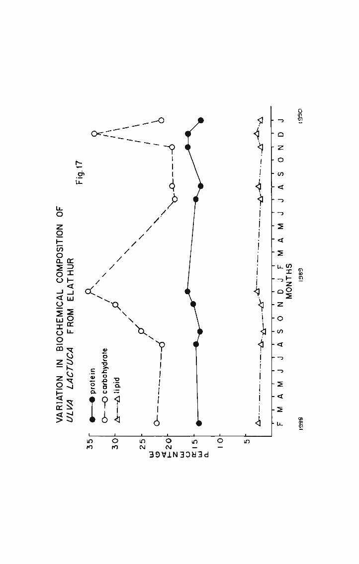
awn.

mzhzoz

.._2<2u_,ozom<

_..-.

h _ b — . . P —

/ L

I |InQ..O/

w ,. T--

4 _ // \ IIIAV

, \

, \ / bx

, ‘ // \\

, \ // Q 23. 4..!fl: / \\ 2o.uEo...tou OI IO% //Ox c_2oR_ I

t .5

m2C<._m .29: YUDKUYQ 8.3.._O zoEmon_s_oo ._<o_2u:oo_m Z. zo:<E<>

I

OIO

L

639VlN33H3d

OON

InNon

man;

9 or.

E&_a.i..42o..EEon.oo O.InO:_o.o:_O|IO

m2¢<.n._ 20¢... 3§s<.E>:\ vtmtofifimvtu

no zoEmon=2oo ._<o_2uxoo_m z_ zo:<_m<>

39V.LN33H3d

118

3.3 8.3 5.2: 3.» 3.9 3.9 .8» $2 woEcEo.5mm.53 .m .m

Eomwocfiww

$2 3.3 8.3 8.” 2.5 3.5 .5... $2 asfia .~

wE8o;o_o

Elm 3.2. 3.3 cm...“ 3.2 8.2 .:E. 33 Sofiao .—

E94 3w._PEoa._w0 E3o.E EQS 3a.6>con._wO 530.5

. cofiowzoo haw? am? we oEmz .02we w2w> 22.530 ..o mmaucoogmm mo 5:22 .5

.=::2m Eoé owmfi E595 wEom mo :o_:moaEoo Eo_Em:oo_m .3 mfiarr

119

3.3 3.? 3.5 23 8...: 85 ..:_<

3.3 3.3 3.2 23 8.3 8.,“ ..::>_ flfislholo

3.2 3.3. 3.3 23 8.2 8.... 5mm 82 2.::_ow._O .m

$2 8.2: 3% SEN 3.3 9%: mo<mm><

3.9 ..._.$ 8.3 .:.~ 8.; 8.2 .:E. 82

8.8 9.5 3.3. 23 8.5 8.3 dam22: 3% $3 25 2.2 3.9 .m:<8.8 3.3 3.; .&.N 8.2 2...: A3.8.2 2.3 3.2. 3.“ 8.5 8.2 >2233 S23. 2.9.. S.” 3.9 23 ..a<3.5 2.3: 3.3 sun 8.? owe ..::>_

3.3 3.3. :2: =3 8.9.. 8.? .93. $2

$4: 3.2: 3.3 22 8.3 8.2 dmm3.2 3.5 8.2. 2.... SEN 3.9 .m:<2.8 3.3 ES 23 22: 8.: A3.8.2 3:3 225 8.” 8.2 2; ..:_<

3.2 8.3: 3.2.. 25 8.3 2: ..::>_ .

3.2 2.2: 3.3 22 8.5 8.2 58 32 E33 .m

_ 8%

3.2 3.2: 8.2. 2.. 3.3 cm.» $02 $2 E:=u:mO .—

2&4 3w..PEon._wU 530.5 E94 muwguzcongwo E3o...m

cosoozoo mm? mo mEmz .ozmo omwucmohwm mo 5:02 Sm» ._m

._o o:_m> 0C_.~O—wU

.=::Sm E9: 2&3 Um: wEom mo :o_:moaEoo Eo_Ew;oo_m

4% came

120

2:32?

2:: m_mmo_U:wO ....

23 3% 5.3 3... 3.2 85 .:E.

2.2 «NS: 3.3 23 3.2 8.3 .89 $2 a._mL::o._ .I. .__.

3.9 3.3. 3.3 22 3.9 and mo<mm><

$5. 8.2 3.3 .:.~ 8.8 8.2 EE. 2...:

3.3 end: 8.8 22 8.2 8.2 .398.2 34:: 33 8.. 8.2 85 .>oz8.9 8.9.. 3.3 22 8.3 8.: dam8.2 3.3 $43 BIN 3.3 8.: A3.8.2 8.8 3.5. 2% 3.5 8.2 .:3.cm? 8.8 No.5 8.“ 8.8 3.2 >328.: 3.3. 2.3 8.. 8.2 8.... ..E<wmfi 3...: 5.2 22 8.2 3.... :52

E4: 3.2. 2.2 o—.N 8.: 85 58 $9

3.3 $4? 3.3 £.~ 3.2 8.2 .353.2 3w: 2.9.. $4 8.: 3...: .>oZ22: £.$ 8.5 22 8...; 8.2 dmm3.2 34$ 2.3 oF.m 8.2 8.: A3.

329 8.2 3.2. o—.N 8.8 3.2 53. .m|awlo_flAu|o

3.3 2.3 3.3 S... 2.4.: 85 3:2 $2 w_..w:ow._O

E95 3w._EEon._mO 530.5 294 muagcmzonpmo E305

cofiomzou Lwww mwfi mo mEmz .ozmo m3w> o_.:._o_mO go %352.& we 5:02 AmA.:B:oOV S oz?

121

3.: 8.2: 3.; 3; 8.3 SE. mo<mm><8.3 8.3 2.3 22 2.2 2.» $2

3.: £2: 3.2 8; 8.: 8.” .22 |I|I2§;o_oa

2...“ $23: 3.3 mm... 3.3 21: ea. $2 £__:mw_o 5

SEN «N3 3.2 :5 3.? $4. mo<mm><8.3 3.3 2.; 8.” 24% S5 .328.3 5.: 3.3 2.... 2.3 cg ..a<

Sam 3.3 8.; 22 mmfi 3...... .32 :||m___na_hm>

8.2 3.8. 2.$ 22 SEN 8.: dam $2 wamoszoo

was B€PEo€mo 589$ 23 3s.6EoEao 589...

COSOOZOO Lmmw mm? Q0 oEwZ .OZmo @3—G> UC_._O—.@O no omwucoopmm .«O £aCO—>_ AmA..._3:oOv S 292.

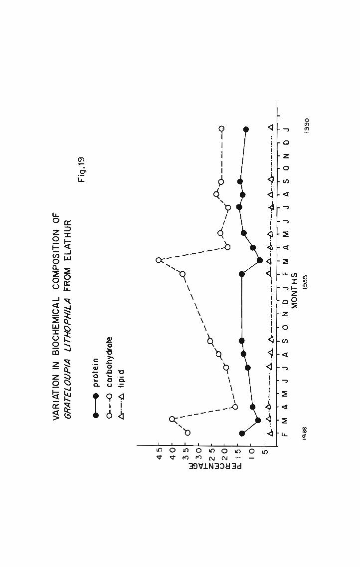
own. mom. Sm.

mxpzoz

_.ozom<_...s_<zuaozom<...._2<s_m

q..l.I.l.|.|.l.Iqu.lq.Au.nI.I|4r...d.|.q.lq'..l. | I . I I ..... |.l¢.|4I.a J @3.1 d\\\C D _ 3/ \ 8T:-.£» 42, up .,, \\O\ , .m NW., \\\ ,. ..OmV/ \\ , b mmm

. \b\ ,o\ o¢

. \ 1

m -5.

E2. 4.!.42EuEo€ou O.I.Oc_2o3 Im:_¢<._m 201.... v7\\In\9£k\.~ §33m§§

.._o ZO_.:mOn=20o ._<o__2u:oo_m Z_ zo:<E<>

mwm. mam.

m.¢zo_2

aozom<_,..s_<s_m_,ozom<.,_.2<2u,T«_..¢..-._-_ .-.-_...,.._...A_».L,T,.T\,_w;_w.-.w- _ ;.T._..- _ .-. ..-¢.-¢.+.-¢-u¢;b..|IO/ \O\.O::O//O

ohm.

6/ \o..o\b,

D/ xwxx dYxV // xxx H\

//ox d\ox

E3. d.|i4o_o::Eon.ou 0.1105205 I

omoa

m:_.:<.G .201... _\.~vG\.R\Q.u §_.:3§x.§.._O ZO_.:mOn=20o ._<o_sn._:oo_m z_ zo:<_m<>

Oo 0IO N39V1N33U3d

122

U_Q: umw3o_ 2: om.U._oow._ mama» 00¢

$9.50. 2: ooo._ooo._ gm? _.:so._m

E305 umm:so_ 2: UmU..ooo._ mam? umm

.E3:oo.2&:. 52» mo um:so=o._ Emzcoo ca: 5.2.? 2: vovhoomn 2&3 Eso._mJcwucoo 3w..EEoo._mo.3»? :$._m >9 _uw3o:£ Emucoo 3w._EEoo._mo m2_m_._ Qt cwv._oom.. 2&3 cam.E3:oo.3»? .52» an 830:8 Eoucoo E395 u2_m_._ 2: uwo._oow.. mam? Eso._m352m 5.moém 3.3 3.3 «Wm 3.3 $5 2&2 B:5.3 3.2. 3.2. $5 3.: 8.3 mam? Esem$3 8.; ES om.m mm.m— 3.3 mam? :mw._U

FEE 3w._EEon._mO. 530.5 UB5 3m._PEon._mO E395

m0 w3w> O_.«_._O__wU

:o_:moqEoo _mo_Ew:oo..m .&

:o_mEo Em?

.S5Em um wmmfi ..o m:o_m_>G

uC®._®.:._U .wO :O_..—_wOQEOO _wo_Eo:oo_m

.3 asap

123

5.1.4 Biochemical composition of some seaweeds from Thikkotti (Tables66-69 and Figs. 21-23)

At Thikkotti, among green algae

Caulerpa fastigiata (February 1989) recorded the highest protein content

of 20% and Q. sertularioides (April 1989) the lowest of 4.1%.

Caulerpa peltata (February 1989) recorded the highest carbohydrate content

of 69% and Cladophora glomerata (May 1989) the lowest of 5.5%.

Caulerpa sertularioides (April 1989) recorded the highest lipid content of

18.75% and Spongomorpha indica (July 1989) the lowest of 1.03%.

Among brown algae,

Padina tetrastromatica (February 1989) recorded the highest protein content

of 18% and Dictyota dichotoma (March 1989) the lowest of 5.2%.

Spathoglossum asperum (January 1989) recorded the highest carbohydrate

content of 17.75% and Padina tetrastromatica (March 1989) the lowest

of 6.25%.

Dictyota dichotoma (February 1989) recorded the highest lipid content of

11.3% and Padina tetrastromatica (March 1989) the lowest of 4.1%.

Among red algae,

Hypnea musciformis (November 1988) recorded the highest protein content

of 14.2% and Gracilaria corticata (September 1988) the lowest of 7%.

Gracilaria corticata (February 1989) recorded the highest carbohydrate content

of 31.5% and Bostrychia tenella (October 1988) the lowest of 12%.

Laurencia sp (January 1989) and Acanthgnhora spicifera (April 1989) recorded

the highest lipid content of 3.3% and Gelidiopsis variabilis (November 1988)

the lowest of 0.8%.

124

2.8 8.8 8.8 8.8 82: 8.2 mo<mm><

8.8 8.:. 8.8 8.8 8.2 8.8 .52. 82

8.8 8.8 8.8 88 8.2 8.2 .858.8 8.8 2.8 28 8.8 8.3 ._3.8.2. 5.8 8.8 8.8 2.8 8.3 ea.8.8 8.8 2.: 8.8 8.... 8.8 828.8 8.8 8.8 8...“ 8.: 8+ .228.8 8.8 8.8 88 8.2 22. .823.8 8.8 8.8 8; 88 8...: .8.._

3.8 8.8 8.8 88 8.2 8.2 as. 82

8.8 2.8 9.3 3;. 8.3 8.: .25 Slammam

8.8 8.8 8.8 $6 8.8 8.5 58 82 3% .8

2...: 8.8 8.: 8.. N: 8.2 mo<mm><2.: 8.8 8.5 8._ 23 8.3 .m=<

88 8.8 2.8 23 N; 8.: ._E. mslofi

8.8 8.8 2.: 88 88 8.5 .5... 82 maflaaamm .N

2.8 8.8 8.2 8.8 2.2 8.2 mo<mm><

8.8 8.: 8.8 8... 8.: 8.8 .8.._ .__..«.=|:

8.8 8.8 8.2 8...” 8.2 8.2 8.. 82 m_E._oE3wm:O ._

EQS 3m._EEon._mo E3o.E E94 3m.6>:on.EO 530.5

COSOOZOO LMGW am? mo OEGZ .OZm0 2:? o:_._o_m0 MO wmmucmogmm no _._u:OS_ Am

_3ov_v_E._. E0...“ owm_w cmmzm ®EOw Q0 CO_w_mOQEOO _m2Em:oo_m .®w 29¢.

125

8.8 8.8. 8.... 8... 8.8 2... 8..2.8 8.3. ....3 2.8 8.2. 2.2 .828.2. 828 8.... 8.2 8.8 8.2 .828.8 8.8. 2.8 8.8 8.8 8... .5...8.2. 3.8. 8.8 8... 8.3 8.2 828.8 8.8. 8.... 2.2 8.2. 2... .3...8..2 8.8. 8.8 3.2 8.8 8.8 ..as_

2.8. 838 2.3.. 8... 8.8 2.... .88 82 8Eo_._2=.._om.w .8

3.3 8.88 8.8 2.8 8.5 8.... m.u<mm><8.8. 838 8.2. 2... 8.8 8.8 don

8.8 8.2a 3.8 8.... 8.8 8.2 .5... 82 fl..._J.._.mm.m .8

8.8 8.88 8.8 8... 8.2. 2.8. mo<mm><2.3 8...: 8.8 38 8.2. 8.2 822.3. 8.8. 3.2.. 2.... 8.8 8.8 .8...8.8 2.2.. 8.8 3... 8.8 8.8 .82

8.8 3.88 8.3 3.6 8.8 8.2 59. 3%.

8.8 8.8 8.3 2.8 8.8 2.2 .2... 82 mmsdm ..

was Bfluéofiao 530.5 29.. o.2.;._o2wo 582..

:o5ow:oo Lwww mm... mo oEmz .oz.«O o3w> U_.:._O~.mO .wO wmwwcmogvm ..o £u_._O—>_ AmA.:3:oOv do w3w.H.

126

8.2. 35$ $3 23 £2 8.: mo<mm><8.3 3.2: 22$ mi 3.2. 8.2 $2

8.8. 8.3m 3.8 33 8.5. 8.: .52. $2 2E._8_=m E3 .m s

53 £5: 2...... $5 m~.~¢ 22 mo<mm><

Sim 8.2: 8.3 8.2 8.2. 23 .52. 8.:

3.3 8.3: $..:. Ea 8.8 3.2 .898.2: 2.2a 2.3 8.: 8.3 8.2 .8222:. 3.8. 3.8 22 8.2 3.: 3.2£52 2.2: Sam 223 3.5. 3;. .a<£52 3.2; 2.2.. 2.: 8.3 3+ 32

2.52 3.8m 8.3 $2. 8.2. 8; 58 $2 mmflozsstom .m

U_Q_Q 3w._PEon._mO :_@aO._n_ EQMJ o..w.6>:on._mO 530.5

:oSom:oo Lmmw am; we mEaz .ozmo w3w> OC_..O~wO mo omwacwohwm mo £u:O_>_ AmA:..3:oOV .8 035

mmm.

mam.

mzpzoz

a_._2<2u__.ozo

0mm.

-m-<-7-3-2-<-2-LL

E2. drlid2o.uEo€oo Oll:O52°... I

5.5

_Cov_v__z» 29.... vbxmmsod vtommoqad....O zoEmon=2oo 4<o_s_u:oo_m z_ zo:<_m<>

“'7 O39VJ.N3DEl3d

C)01

H1G1

mm“. «mm.

mzpzoz

::_m_

— _

omm_

Dbxb, \\ /

\

\\ / w \ /2

m \ , \ / \ o.b

\ / \\ z \ , \C \\ I’

Q / \\ K X \\ yu

/ \ I \Q‘ 2Q:ar;!L , \\

o_2vEon.ouOI|.|O T

c_£o.n_ I

NNoC

_Cov_v_._._» s_oE mm9oE3\:mmm _\nEm.S§.._o zo_:mon_2ou ._<o_2mxoo_m z_ zo_»<E<>

9O O 0<1’ :0 N39VJ.N3C)H3d

0Lnom

127

3.8 8.3 2...: $5 $9 3.9 mo<mm><

8.8 3.5 3.5. 3.3 3.3 3.9 58 .|g|E=._ ma

3.; 3.3. 3.2 35 £22 3.: £2. 2:: Esmmoaocfimm .m

2.3 3.3 3.3 2.3 8.: 3.3 mo<mm><3.2 $2 3.3 3... 35 Se ..:2>_

$3 8.3 22:: £2 3.? 8.3 .%r._ wo5aEo.:ww.:.3

2.3 8.3. 3.8 $5 3...: 8.2 .>oz $2 26.3 .m

3.8 3.2. Sém 2a S4,". S5 mo<mm><2.8 5.5 3:8 85 36 can ..::>_3.2: 3.2.. 8.3 3.: £5 2...: dam

3.3. 3.2. 3.9. 85 8.2 85 E2. 2...: wE3o:o€

3.8 3.2 5.3 8.2 8...: 3.3 .>oz 2:: Sofofi .—

E34 3a._EEon._mU 530.5 2&4 3w._EEon..wO :_.3o..m

cozowzoo EMS am? we wEmz .oz.8 33> o_.:._o_wO mo wmmucmohwm mo 5:22 .5

_3oxv=F_. Eo.c 2%; E595 mEom mo :o_:woaEoo _wo_Eocoo_m .3 flame

128

2.: 88.88 88.88 2; 88.; 88.8 mo<mm><

8.2 88.8: no.3 88.. 88.88 88.8 .888 882

88.: 8.88 3.3 88.. 88.88 88.8. .8288.2 88.88 88.88 2.2 88.2 8.8 88288.2 2.88 88.; 85 88.2 2.8 ..a<88.8 88.82 88.88 88.8 88.88 88.2 .88288.2 2.82 88.88 2; 88.28 88.: .88

88.2 88.82 3.3. 85 88.88 88.8 .888 882

88.2 88.28 88.2. 2.. 88.2 88.8 .8288.8 88.88 mc.w_¢ 88.8 88.88 88.8 .8088.8 88.88 88.88 88.8 88.2 88.8 .888

8.8 3.3 88.88 88.8 88.2 88.2 .882 3

8.8 88.82 88.88 88.8 88.88 88.2 .88 882 822620 .82.2 2.882 88.3 88.2 88.88 88.2 .888 882 .88 88%: .8

m_E..otom:E

88.8 88.88 mmém 88.8 8.88 88.2 .82 882 82.1%: .8

E::_m:m

8.2 88.82 88.8 85 2.88 88.8 .82 882 E:_E_mO ._

E83 3w.::Eon._wO 538.5 283 3w._U>:on._mO E3o.£.

cofiomzoo Sm» am? mo mEwz .ozmo m:_m> OC_._O_wQ mo wmwucwohom «O £u:O_>_ Am

_3ov_v_E._. E0...“ 2&3 00.. mEom mo :O_u_mOQEOU _mo_Eo:oo_m_ .ww 0_Dw(—.

129

wzocmz

22.. 8.2. 3.3 22 8.9 8.2 .30 $2 aE%.:mom 5

3.8 3.; 3.3 Ea E29 2...: mo<mm><3.2 3.3 9.: 21.. 3.2 Sf 2328.3 3.3. 3.3 23 8.2 3.3 ..E<3.2 8.8 3.3 22 8.2 3.2 .8m

$4: 8.8 3.8 Q3 3.9 22.. .:E. $2 llm..m._w.:o_ m

8.3 3.8 3.3. 8.” 8.2 8.2 .>oZ 2:: So._mo£=8< .w

3.3 3.3. 3.8 S.» 3.2 3.: mo<mm><3.2 3.2: 3% 3.“ 8.8 3.: den

3.; 8.2: 3.3 3.” 8.3 3.9 .:a_. 2:: dm m_o.._w._=mA .~.

3.2 22$ 3.3. 3.4 8.; :3 mo<mm><$5 8.8 3.3. 3.. 8.3 and 43..3.2 2.8 5.3 2.. 8.3 S5 .55.3.3 .222: 3.3 22 8.3 85 >22

2.2 mmé: 9%; .22 8.8 85 .8.._ |m_nwfi:o_ow

2.; 3.2: 3.3 8... 8.3 owé .52. $2 m:5..wm_U .m

m:Em_._w>

was 3.2: 8.2. 8... 2.3 22 .>oZ 2:: m_mmo:u:o_O .m

E94 3m._EEon.EO 530.5 E94 3w._EEon._wO E3o...m

:o:om:oo pwww aw? mo wEwz 62mo w:_m> o_.:._o_wU mo mmaacoohvm mo 5:02 .5A....B._o8 .8 osfl.

on? own. mum.

_._.._.Oxv:_._._. 20¢... VRVGCQQU 3....€§§G.._O zoEmon__2oo ._<o_s_H._:oo_m z_ zo_»<_m<>

mI._.zo_2

3 a Z O m < 3 a 2 < 2 u a o 2 O m 4 3 a 2 < 2 u

. I . | . .|u. <.l

\.\<|l..| Id/. .\ <// .\.\d«

l .b, 0.1: II

\\ \ A \ IIIIO 1

\\ a \ ,\\\ . \ ,

xbx , u ,

\ . xxox ,,

\ . \ 1

Ox ._ \ o.a.c».._o.:ou O.|I.O ,&

.0 Awx c_2oE I .8.9“. .

O10O(\|

O In|-0 N39V.LN33H3d

IDI0

130

.u:w«:ooU_Q= amm:so_ Qzu uwchoowh gm? uwm dam? CGQLM >3 om:so=o.. Emzcoo Umflmm um0£.w__._ OF: UOULOOOL mam? :30._m

.u:w~:oo wuahozconhmoumw3o_ Op: UQULOOOL cam? C>>OLm .wwm_w Um: U®>>O=O.u u_._0uCOO ouwhvzconnwo um0£M_£ m5 UOULOOQL mam? EOGLO.u:wa:oo:_0uO._Q umm..so_ m5 UOULOOOQ mmmfi DON .0wM—w COOLM >0 —U@>>O=O.« acwucoo =_®u0.—Q umo:wE 0...: UQULOUQH wwmfi :>>O._m._:8_v_E._. 28.2 3.3 Si 8.. $.§ $5 2&2 Ex3...; $3 8.8 :3 5.: 5.: 2&2 Ezzm:5. 8.5. 2.2. 5.5 2.; 8.: mam? :85

29.. 32EEo€ao 530.5 Ea: o::EE8.:.o £82m

co_m_>5 Em?

«O 0=—6> O_.«_LO~.mU r_O_..:mOQF_OO _.mo_Ew:oo_m mm

_HHOv__v__£,H um mwmcm MO m:o_m_>_v u:w.~Q.u.:U mo COCEOQEOO _mo_Ew;oo_m .m© 293.

131

5.1.5 Biochemical composition of some seaweeds from Saudi (Tables70-72 and Figs. 24-26).

At Saudi, among green algae,

Enteromorpha compressa (September 1988) recorded the highest protein

content of 13% and Chaetomorpha antennina (March 1989) the lowest of

5.1%.

Enteromorpha compressa (August 1988) recorded the highest carbohydrate

content of 27.75% and the same species in March 1988 and June 1988

recorded the lowest of 6.75%.

Chaetomorpha antennina (April 1988) recorded the highest lipid content

of 7.35% and Enteromorpha compressa (April 1989 and December 1989)

the lowest of 1.2%.

Among red algae,

Grateloupia filicina (November 1988) recorded the highest protein content

of 18.6% and Centroceras clavulatum (June 1988) the lowest of 7.6%.

Grateloupia filicina (August 1988) recorded the highest carbohydrate content

of 55% and Centroceras clavulatum (June 1988) the lowest of 14.25%.

Grateloupia filicina (May 1988) recorded the highest lipid content of 2.85%

and Q. filicina (November 1988) the lowest of 0.85%.

132

....8 8.8 8.8 2.. 8.2 88 .52

8.8 8.8 ...8 8... 8.2 8.8 .8... w

8.2.. 2.8 8.8 8.8 8.... 8.8 8.. 82 mm .~

...2 ...N. 8.8 8.. 8... .88 mo<mm><8... 8.2. 8.8 8.. 8... 8.2 .258.8 8.8 8.8 8.8 8.8 8.8 8m8.8 8.8 2.8 8.8 8.8 8.8 .838.8 3.8 8.8 8.8 8.8 8... .3.8.8 8.8 8.8 8.8 8.8 8.2 .5...

8.2 8.8 8.8 2... 8... 8.2 .....s_8... 8.8 8.8 8.. 8.8 8... .2...

2.... 8.8 8.8 8.. 8.8 8.8 .32 82

8.2 8.8. 8.8 88 8.8 8.2 .808.2 8.8. 8.8 8.8 8.8 8.2 4.82.3 2.2. 8.8 8.. 8.8 8.2 .8...8.2 8.8 8.8 2... 8... 8.. .3.8... 8.8 ...8 8.. 8.8 8.... .5...

2.3 8.8 8.2. 8.. 8.8 8.8 .32 O|U

8.2 .28 8.8 88 ..:..w 8.8 .82 82 mafia ..

23 3EPEo€ao 582.. 23 8223880 53?.

.._O 03_d> 2280

..o mm3:mo.5m

:o:om:oo .8;

mm? ..o oEmz .oz.0 5:02 Am

Baum E0...“ mam? cwmzm ®EOw .wO C0_u_mOQEOO _mo_Em._oo_m

.3. 293

133

8.3.. 3.3 8.3 3... 33.2 33.3 mo<mm><33.3 33.33 33.3 8.3 3.2 3.3 .8933.3 3.: 33.3 8... 3.: 8.3 5oz33.33 33.33 2.3 8.3 8.3. 8.3 .6033.3 3.:. 33.3 8.3 8.2 8.3 .3332.33 2.33 2.: 33.3 3.2 8.2 .33

8.2 8.2. .38 8.3 8.2 8.3 .833.2 8.2. 3.33 2.3 8.2 8.2 33233.; 3.2. 8.33 33.3. 33.2 8.3 .833.33 3.:. 33.33 3.3 8.2 2.3 .3328.33 33.33 3.33 8.3 3.3. 8.2 .333

23.3 33.33 2.; 3.3 3.; 33.2 .533 332

3.33 33.3 2.: 33.3 33.2 8.2 .893.3.3 8.3 3.33 8.3 8.2 8.2 .323.3 33.3 33.3 8.3 8.3. 8.3 .803.3 33.33 8.3.. 8.3 8.: 8.3 .3333.3 3.3. 33.2. 8.3 8.2 33.3 .33.2.23 3.3 33.2. 3.3 3.: 3.3 .333.33 33.3 3.8 2.3 8.2 2.3 .32.

3.33 33.3 3.3 2.3 8.2 3.3 332 3%8.33 33.3 5.2. 33.3 8.2 3: ..a< 332 3%

E33 33._PEon.:3O 5823 was 83533330 530.5

cosoozoo .335 33: mo mEwz .02mo w:_w> O_.:._O—.mO HO mwmucoopwm mo £w:O_>_ Am4:3 :oOv .3. 235%

awn...

0mm.

mxkzoz

..ozom<.. .._2<s_“_..ozom<_,_.s_«2.._

.m.o_.9

/

\\O/dr xbx / \\ Lou

\ .Q //

\\ dxbx \ Lmm

Q 22. 4!l.LQ d

2o.uEon.ou OIIIO Lon

522.. I

vmar. -3

.33 22: qmmmtmfiou wtmmozotmxzmn_O zoEmoa_2oo ._<o_2m:oo_m Z_ zo_»<_m<>

39VJ.N33H3d

mum.

m_¢zos_

ozom<....s_<2u__.oz— - - P

8.0:

Ba: d...I.LQ

2o.EEon.ou OIIIO 1

c_2oE I

_o:<m 20¢... Y>\\\<\<W.~\<_\ v\In\n<Q3.QkN3.>u.._o zoEmon_s_oo ._<o__2$_oo_m Z_ zo_»<_m<>

OIDI0 Oc\: N39V.LN33B3d

0r0

134

3.5 8.: 3.2. 8.. 9.3 one mo<mm><

2.3 3.3 §.fi. cmé 2.3 em.» .:=_. 3.: |.|E:uw_:>w_o

:2: 8.3 3.8 2.. 8.8 85 £3. 2:: ma..mow.5:oO .m23: 3.2: 3.: 22 3.3 8.2 5mm 2:: 2Emo5= W .N

2.2 $52 ww.Nm 3.. 3.8 3.3 mo<mm><3.2 3.8 3.8 8.. film 8.2 .11..3.2 $.E 3.3 22 3.2 8.: ..::>_

2% 3.3. 8.8 8; 8.3 8.2 58 $2

3.: 3.2. 3.8 9..., 8.2.. 8.: .omQ23 $.24 3.2: 3... 3.3 3.3 .>oz$1: «$2 8.3 8; 3.5 8.... J008.: 8.2. 3.3 8; Sam 8.: dew3.2 34.2 3.3 22 8.3 3.2 .m:<2.8 3.9.: 2.3 $2 8.; 3.: >w_>_23 34.2 5.2. 35 8.2.. 2.: :82

22: mfiofi 3.2. 8.. 8.3 8.2 dam I||I|wEo:£

8.: 3.2. 3.2. 3.. 8.3 3...: £3. 32 Em:o_3m._O .—

UB3 3w..EEoo.:w0 E305 E94 w§._PEon._wO E305

cofiowzoo ._mm% am; we oEwz 62..o 2:w> o_.:..o_mO mo wmaucwonwm We 5:22 .5

Ezwm E9: 2%: cm: wEom ._o :o_:moaEoo _mo_EmEuo_m .E. wfimp.

gh.

wzpzoz

ozom<....s_<_2..__.ozom< ..s_<2..__..

4|.|.|.|.I.Q.LQ/.I.:d...\dr.dr..dr.drI.I.I.a4\.\.\dr..d_...4

-m-o_..m_-o~.3

E5. d.!l.LQ K

2223023 olluo -on

E3o:.O|||O

-nm

8.0:

_o:<m 20¢... v‘>\>u3\u.\ 3nS3.E§.m.._O zo_:mo&2oo ._<o__2m:oo_m Z_ ZO_._.<_m<>

39VLN33H3d

135

swam? own :9: E3:oo Ea: mo o..oE Uou._oom._ 39¢ cmmzo.$m:.. :wm._m :9: Eoucoo 3m..EEoo._wo ocw E3o.a go o._oE umv..oom._ mwmfi omm._o_am u<8.2. 3.6: 3.: 3.. 2.2 $5. Sm? Em3.4% 3:2 9.3 8.... 3.2 85 mam? :85

E94 3m._PEon.EO E395 UB5 3w..U>;o..._._wO E3o._m

.«O w:_m> U_.:._O~mO :O_w_mOQEOO —GO_F_®£UO_m mw

:2m_>5 Em?

Ezwm um mam? mo m_._o_m_>_U :._m._w...:v Q0 :O:_mOQEOU _wo_Em:oo_m .N~. Bomb

136

umm:so_ 23 .=..=:—>_ DEG Eoucoo 3w._PEon..wo umm:so_ OF: UOULOOGL Ezwm

ca: new 3w..EEoo..mU

Jcmzcoo Ea:._3ov_xE,w um ..mw;mE O._0>> macoucoo

.E:E_EE .2: w:$_..m> baa Emzcoo 530.5 E:E_xwE of Uou._oom._ 552m

Jam? 52m Low

32% 3.8 8.5 S... 5.2 5.2 mwm._w><

3.3 2.3 2.5 E...” 8...: 85 Ezam .m:22 8.5 3.3 8.” 3.2 3.: .=..E.Sm .«5.3 3...? 2.8 pm.» 3.; 8.: _5ov_v_EE .m:2.“ 3.3 2.3 :2 5.9 :3 Emv_.E> .m

SEN $5: 8.8 $.N 2.5 $5. .5232 .—

E95 3m.6>:on._mO E3o.E EQE 3m._P_Eon._wO E395

cosfim .ozmo w3a> 2.2.530 no wmwacmohom ._m

Hmwoo w_mzmv_ mcofi mcofiwum Em._w.:€ E9... mam? 52m .3 :o_:moaEoo _mo_Em:oo_m_ .3. Bomrr

137

33:32 U33 33:00 En: 3mo._mE 05 o%._o8._ _3ov_v_E._.

.3330. 2.5Jmm3o_ 9: ._3:32 3:3 Emzcoo 3a._EEon._ao

um2_mE m5 U®U._OO0._ 2av_..a> .umo3o_ OCH w_$_._a> USN Emzcoo _.:0uO._Q umm:mE 2: 32003 ._352m

6393 Eso.E ._o.m

Sam 3.? 3.3 $5 3.: 2.:3.3 8.2. «Tm» 24.4. 5.: 8.33.2 $43. 8.8 :3 :..: 3.:

3.3. 8.3 _.m.$ 3.6 :4... :...m3.3 8.3. 8.3 55 35 $5

mo<mm><

._3:uSm .3”_:8_V_Ee .mE$_._w> .m33:32 4

582m 293 3.223850 £82m

2&3 82u.Eo£ao

.30 33> OC_._O—GU mo mmaucmopwm

cosfim .oZ.5

umaoo Egon MEG?» mcofimum a:@._Q.u.:U EO.C @393 :>>O._D mo CO_u_mOQEOO _mo_EmEoo_m

.3. 255

138

.E8:o... Em: um2so_ 2: 8282 _3ov§E._.can Baum Jcmzcoo 3m._PEon._wo $252 2: ._:::E E5 Ewucoo E395 um9.so_ 2: voupoomg 29_.S>

Jcmucou ca: §._m_._ of .=.=:_>_ 9:. .3:3:oo 3a._EEon._wo 93 530.5 .8__w_._ 9: uwuhoomg Eswm

.$m_a own .5»

3.2 5.8 2.3 8.. 3.3 8.2 mo<mm><

8.3 :65 3.: 8.. $4.2 $5. 6:8 .m8.5 2.8 3.3 Ea Si 85 S._§m ._.8.5 3% 2.3 8.. 3.; $5 Eoize ..e.8.2 2.3 3.5 3.. 2.2 new 28:5 .~:23 3.: 8.3 $.N 3.: 2.3 5:22 ._

U35 ozzoéofiao 5395 2.3 o::EE8.so Esoi

cofiwuw .02mo m:_w> oC_._O~wO ..o omflcwohmm Am

umwoo m_w._wx m:o_w mcofimum u:@._®.:_U E9: mmmfi om: «O :O_u_mOQEOU ~wO_E0£UO_m .m~. Bnmp.

139

3.. 3.2 3.2 35 3:3 3.: 54. ES 5.? mo<mm><3; 9.3 $42 n - I 35 3.3 85 ism§.m 3.2 $5 $5 5.: 3.3 84” 3.2 3.: azzam

8.. 3.; $5 5;. 5.: :3. 5.» $2; 8.: _3ov_v_E.H2.; 8.2 mg 34. E29 56 :2 2.? 3d 2$_..m>22 5.2 2.2 36 35 $5 $.~ 2.5 3.: .=..=:_>_

E94 3m.:.:Eon.EO E305 2&4 3w.6>coo._mO 530.5 294 3w._EEon._aO 530.5

2&2 com 2&2 Esoem mam? :mw._O :oS3w

awwoo Smawx w:o_a wcofigm uC0._@.:_U :_ mam? HO m:o_m_>_U u:®._0.:_U mo CO:_wOQEOU ~GU_E®_._OO_m~

.2. 255

140

At Mullur,

Both green and red algae recorded high protein contents of 10.62% and

10.23% respectively.

Green algae recorded the highest carbohydrate content of 27.33% followed

by red algae with 17.91%. Brown algae recorded the lowest carbohydrate

content of 9.75% .

Brown algae recorded the highest lipid content of 3.87% followed by green

algae with 2.89%. Red algae recorded the lowest lipid content of 2.49%.

At Varkala,

Brown algae recorded the highest protein content of 9.37%. Both green

and red algae had almost the same protein contents of 8.87% and 8.33%

respectively.

Red algae recorded the highest carbohydrate content of 22.20% followed

by green algae with 19.17%. Brown algae recorded the lowest carbohydrate

content of 13.71% .


algae with 2.94%. Red algae recorded the lowest of 1.71%.

At Thikkotti,

Both green and brown algae recorded high protein contents of 11.05% and

11.84% respectively. Red algae recorded the lowest protein content of9.59%.

Green algae recorded the highest carbohydrate content of 31.79%, followed

by red algae with 21.53%. Brown algae recorded the lowest carbohydrate

content of 11.71%.

141



At Elathur,

Brown algae recorded the highest protein content of 14.06% followed by

green algae with 11.45%. Red algae recorded the lowest protein content

of 9.66%.

Red algae recorded the highest carbohydrate content of 22.53% followed

by green algae with 19.52%. Brown algae recorded the lowest carbohydrate

content of 11.17%.



At Saudi,

Red algae recorded a higher protein content of 13.69% while green algae

recorded only 9.06%.

Carbohydrate content was also higher in red algae 28.13%. Green algae

recorded only 15.26 % .

Lipid content was higher in green algae with 3.7% and red algae recorded

only 1.66%.

Thus, along the Kerala coast,

Brown algae recorded the highest protein content of 11.3%. Both green

and red algae recorded almost the same protein content of 10.2% and 10.3%

respectively.

142

Both green and red algae recorded high carbohydrate contents of 22.6%

and 22.5% respectively and brown algae the lowest of 11.6%.


algae with 4% and red algae the lowest with 1.9%.

5.2. SEASONAL VARIATION IN BIOCHEMICAL COMPOSITION OF SOMESELECTED SEAWEEDS FROM VARIOUS STATIONS ALONG KERALA

COAST

5.2.1 Seasonal variation in biochemical composition of some selectedseaweeds from Mullur

From Mullur, 3 species each of green, brown and red algae were

selected for this study. Average biochemical composition of each species,

during the different seasons are given in Table 77. Statistical analysis

(Analysis of variance 1 way classification or ANOVA-I) was done to test

the significance of the observed seasonal variations and the results are

represented in Table 78.

144

ca: : A 2 3a..PEon.:.o .. O m 530.5 n m

23 2.2 2% 2% 8.2 5.» 22 3.2 22 am Mafia2...” 3.2 3.2 23 :4: 2.2 8.” 8.: :3 88852: 32%.3 2.2 24.2 8.. 3.2 21; 22 3.: 844 am? 4.2524. 2.4 22. £4. 2.... 222 E4 2: 3.6 wflvmmwaw mam8... 8.2 2.2 2.... 3.2 2.: :3 2.2 2.2 3%. ga35 3.2 3.2 §.~ $5 $4. 25 8.2 $44 ucaflmmfl24" 2.3 2...: 2.4. 5.2.. .2444 23 222. $2 may a|&m_|=.&2.». 234.. 3.2 $2 3.: 2..., 2.4 3.: 84. 4% .m

2% 24.2 3.2 22 3.2 3.: $2 242 :2 4% S5

4 o m 4 o .4 4 o .4

:oom:oE umom :oom:o_>_ :oom:oE 95 mmfiw mo mEmz

mcomwom Eo._w.C€ 9: m.__.=.u .=4:3>_ E9: mumwzwom mo :o_:moaEoo _mo_Ew;ooE mmm._m><

SN. 2%?

145

Table 78. Significance of seasonal variation in biochemical compositionof some seaweeds from Mullur based on statistical analysis

Name of alga Remarks based on statistical analysisProtein Carbohydrate Lipid

fig fasciata HI.SIG N.S. HI.SIGE. lactuca HI.SIG HI.SIG N.S.Caulerga geltata N.S. N.S. HI.SIGSargassum wightii N.S. N.S. HI.SlGChnoosgora minima N.S. N.S. N.S.Em gymnosgora N.S. N.S. HI.SIGHygnea valentiae Hl.SIG N.S. N.S.Sgyridea filamentosa N.S. N.S. N.S.Gracilaria corticata N.S. HI.SIG N.S.

HI.SlG - Highly Significant ; N.S. - Not Significant

ANOVA Tables of the biochemical constituents that showed significantseasonal variation are given below:

Table 79. Variation in protein content of Ulva fasciata from Mullur betweenseasons.

SOURCE D.F. SUM.SQR MEAN.SQR. F-VAL REMARKSTREAT 2 143.223 71.611 6.96 HI.SIG(1%)ERROR 18 185.30 10.294MEAN COMPARISONS REMARKST1 - T2 SIGT1 - T3 SIGT2 - T3 N.S.HI.SIG - Highly Significant ; SIG - Significant ; N.S. - Not SignificantT1 - Pre monsoon ; T2 - Monsoon ; T3 - Post monsoon

146

Table 80. Variation in lipid content of Ulva fasciata from Mullur betweenseasons


TREAT 2 2.154 1.077 7.34 HI.SIG (1%)ERROR 18 2.642 0.147

MEAN COMPARISONS REMARKST1 - T2 N.S.T1 - T3 SIGT2 - T3 SIGN.S — Not Significant ; SIG — Significant ; HI.SIG - Highly SignificantT1 — Pre monsoon ; T2 - Monsoon ; T3 — Post monsoon

Table 81. Variation in protein content of Ulva lactuca from Mullur betweenseasons


TREAT 2 371.148 185.574 29.67 I-II.SIG (1%)ERROR 18 112.569 6.254

MEAN COMPARISONS REMARKST1 - T2 SIGT2 - T3 SIGT2 - T3 SIGN.S. - Not Significant ; SIG - Significant ; 'rII.SIG - Highly SignificantT1 - Pre monsoon ; T2 - Monsoon ; T3 - Post monsoon

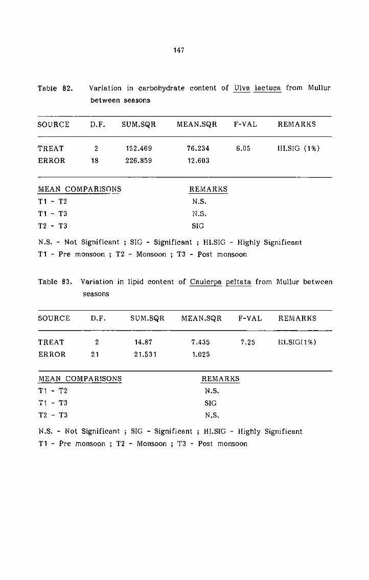
147

Table 82. Variation in carbohydrate content of Ulva lactuca from Mullurbetween seasons


TREAT 2 152.469 76.234 6.05 HI.SIG (1%)ERROR 18 226.859 12.603

MEAN COMPARISO1_\I_S REMARKST1 - T2 N.S.T1 - T3 N.S.T2 - T3 SIGN.S. - Not Significant ; SIG - Significant ; HI.SIG — Highly SignificantT1 - Pre monsoon ; T2 - Monsoon ; T3 - Post monsoon

Table 83. Variation in lipid content of Caulerga geltata from Mullur betweenSEBSOHS


TREAT 2 14.87 7.435 7.25 HI.SIG(1‘/'6)ERROR 21 21.531 1.025

MEAN COMPARISONS REMARKST1 - T2 N.S.T1 - T3 SIGT2 - T3 N.S.N.S. - Not Significant ; SIG - Significant ; HI.SIG - Highly SignificantT1 - Pre monsoon ; T2 - D/Ionsoon ; T3 - Post monsoon

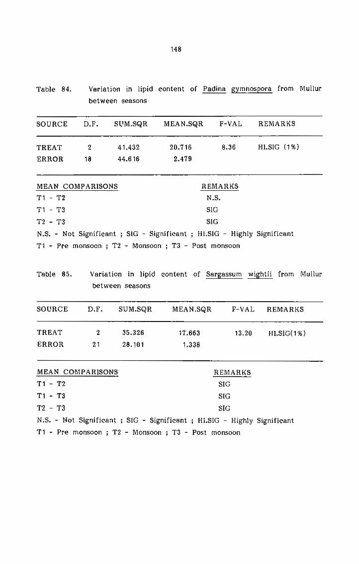
Table 84. Variation in lipidbetween seasons

content of Padina gxmnosgora from Mullur


TREAT 2 41.432 8.36 HLSIG (1%)ERROR 18 44.616

MEAN COMPARISONS REMARKST1 - T2 N.S.T1 - T3 SIGT2 - T3 SIGN.S. - Not Significant ; SIG - Significant ; HI.SIG - Highly SignificantT1 - Pre monsoon ; T2 - Monsoon ; T3 - Post monsoon

Table 85. Variation in lipid content of Sargassum wightii from Mullurbetween seasons


TREAT 2 35.326ERROR 21 28.101

13.20 HI.SIG(1%)

MEAN COMPARISONS

T1-T2T1-T3T2-T3

REMARKS

SIG

SIG

SIG

N.S. - Not Significant ; SIG - Significant ; HI.SIG — Highly SignificantT1 - Pre monsoon ; T2 - Monsoon ; T3 - Post monsoon

149

Table 86. Variation in carbohydrate content of Gracilaria corticata fromMullur between seasons

SOURCE D.F. SU1‘.'I.SQR MEAN.SQR F-VAL REMARKS


MEAN COMPARISONS REMARKST1 - T2 SIGT1 - T3 SIGT2 - T3 N.S.N.S. - Not Significant ; SIG - Significant ; HLSIG - Highly SignificantT1 - Pre monsoon ; T2 - Monsoon ; T3 - Post monsoon

Table 87. Variation in protein content of Hynea valentiae from Mullurbetween seasons



MEAN COMPARISONS REMARKST1 - T2 SIGT1 - T3 SIGT2 - T3 N.S.N.S. — Not Significant ; SIG - Significant ; HLSIG — Highly SignificantT1 - Pre monsoon ;_ T2 - Monsoon ; T3 - Post monsoon

150

5.2.2 Seasonal variation in biochemical composition of some selectedseaweeds from Varkala

From Varkala, 3 species of green algae were selected for this study.

Average biochemical composition of each species during the different seasons

are given in Table 88. Statistical analysis (Analysis of variance 1 way

classification or ANOVA-I) was done to test the significance of the observed

seasonal variations and the results are represented in Table 89.

151

:__8cEm_m 2:9: - o_m.E N ::§:._m_m Sz - .m.z05.5 .m.z .m.z mE::3:a a;m._oE3oa:O

.m.z 05.5 .m.z 832: .m

.m.z .m.z .m.z 320%.. 9::

23 3EEEo£ao 530.5

Embaca Eozmfiflm co comma mv_..wEom

$3 mo oEmz

2av_.E> EOLH muwozawm couoflwm 0EOm .wO :o_:moaEoo —wO_E0£OO_D :_ :oEm_.E> Ecommwm mo 0UCdUC_:.w_m

wfibacm Bosmsfim :0 uwmwn

.3 mfiwp.Ea: : A W 3w._EEon..mo u 0 N £303 a mw:E:3:m2.». Sam 3...: 23 3.? :3 :6 8.2 m3. Em._oEo$9_o

$5 5.3 $5 i.N 8.5 mg $.~ 3.5 $5 3302 5:

36 3% 3.: «ma 3 .§ «NA: 36 «mam Ed 3233 mi:

4 O m A U m A O m

wmfiw no mEmz

:oom:oE amom :oom:oE cOOw:OE PE

mcomwwm uC@._O.:_U 9: .w:_._3U 3wv_.:.> EO.C mvmmzsmmm ugoflmm mo :o_:moQEoo ~.mO_Ew£UO_D wmm.5><

.3 Bomb

152

ANOVA Tables of the biochemical constituents that showed significant

seasonal variation are given below:

Table 90. Variation in carbohydrate content of Ulva lactuca from Varkalabetween seasons

SOURCE D.F. SUM.SQR MEAN.SQR F-VAL REMARKSTREAT 2 363.621 181.811 7.93 I-II.SIG(1%)ERROR 21 481.443 22.926

MEAN COMPARISONS REMARKST1 - T2 SIGT1 - T3 SIGT2 - T3 N.S.N.S. - Not Significant ; SIG - Significant ; HI.SIG - Highly SignificantT1 - Pre monsoon ; T2 — Monsoon ; T3 - Post monsoon

Table 91. Variation in lipid content of Chaetomorpha antennina fromVarkala between seasons


TREAT 2 6.764 3. 382 7.75 I-II.SIG(1%)ERROR 21 9.163 0.436MEAN COMPARISONS REMARKST1 - T2 SIGT1 - T3 SIGT2 - T3 N.S.N.S. - Not Significant ; SIG - Significant ; HI.SIG - Highly SignificantT1 - Pre monsoon ; T2 - Monsoon ; T3 - Post monsoon

153

5.2.3 Seasonal variation in biochemical composition of some selectedseaweeds from Elathur

From Elathur, 3 species green algae and 1 species of red algae

were selected for this study.- The average biochemical composition of

these selected seaweeds for the different seasons are given in Table 92.

Results of the statistical analysis (Analysis of variance 1 way classification

or ANOVA-1) done to test the significance of the observed seasonal variation

in biochemical composition are represented in Table 93.

154

§.o_:=m_m 3:9: - 23:

m E8:Em_m Sz - .m.z.m.z .m.z O_m.E Swfltoo 2.82020.m.z 05.5 wag: w:E:3:m a.E._oEo$w:0

.m.z 05.5 23: mozuofl WO_m._= O54: .m.z 320%.. «.3:

was o§..P_Eon._wO 5.30.5

m_m3m:a Eosmfifim co ommwn mx._mEwm

aw? mo mEmz

.===2m C._O.C mummxsawm @3028 0EOw Ho :O_u_mOQEOO ~.@U_E®£OO_D F: :o5w_.E> Bcomwwm mo 0U:wOC_:M_w

m_m3w:m Eofimsfim co comma

.8 035.ca: u A M 3w.6>:oo.Eo . O m E3o.a u mEwochoo92 3.2 8.2 w—.N 8.2 8.5 22 $23 :6 w_._w:ow._Ua:E:3:a22 SE 3.? mg :2 “NA: Sam 85 32. m:m..oE3ow:O

mg 8.2 3.2 mg 3.9 3.3 23 %.E 529 3303 W

25 8.3 8.3 ofim 8.3 3.3 up... 3.3 3.5 328$ m>5

A O A 4 O m 4 O m

aw} mo mEmz

:oom:oE “mom :oom:o_>_ :oom:oE PE

mcommmm Em.$.:_c 2: maize SEEM

F_O.C mvowzwwm 9302mm Ocu no :O_u_wOQEOU ~wO_E®£UO_D @.w.®L@><

.3 03¢?

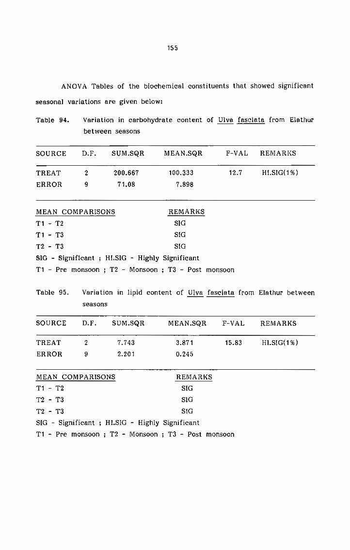
155

ANOVA Tables of the biochemical constituents that showed significant

seasonal variations are given below:

Table 94. Variation in carbohydrate content of Ulva fasciata from Elathurbetween seasons

SOURCE D.F. SUM.SQR MEANM.SQR F1-VAL REMARKS


MEAN COMPARISONS REMARKST1 - T2 SIGT1 - T3 SIGT2 - T3 SIGSIG - Significant ; HI.SIG - Highly SignificantT1 - Pre monsoon ; T2 - Monsoon ; T3 - Post monsoon

Table 95. Variation in lipid content of Ulva fasciata from Elathur betweenseasons


TREAT 2 7.743 3.871 15.83 I-iI.SIG(1%)ERROR 9 2.201 0.245MEAN COMPARISONS REMARKST1 - T2 SIGT2 - T3 SIGT2 - T3 SIGSIG - Significant ; HI.SIG - Highly SignificantT1 - Pre monsoon ; T2 - Monsoon ; T3 - Post monsoon

156

Table 96. Variation in protein content of Ulva lactuca from Elathur betweenseasons



MEAN COMPARISONS REMARKST1 - T2 N.S.T1 - T3 SIGT2 - T3 SIGN.S. - Not Significant ; SIG - Significant ; HI.SIG — Highly SignificantT1 - Pre monsoon ; T2 - Monsoon ; T3 — Post monsoon

Table 97. Variation in carbohydrate content of Ulva lactuca from Elathurbetween seasons



MEAN COMPARISONS REMARKST1 - T2 N.S.T1 - T3 SIGT2 - T3 SIGN.S. - Not Significant ; SIG - Significant ; HI.SIG — Highly SignificantT1 — Pre monsoon ; T2 - Monsoon ; T3 - Post monsoon

157

Table 98. Variation in protein content of Chaetomorpha antennina fromElathur between seasons

SOURCE D.F. SUM.SQR. MEAN.SQR F-VAL REMARKS



Table 99. Variation in carbohydrate content of Chaetomorpha antenninafrom Elathur between seasons

SOURCE D.F. SUM.SQR MEAN.SQR F-VAL REIVIARKS

TEEAT 2 11.113 5.557 17.58 HI.SIG(1%)ERROR 15 4.741 0.316MEAN COMPARISONS REMARKST1 - T2 SIGT1 - T3 N.S.T2 - T3 SIGN.S. - Not Significant ; SIG - Significant ; HI.SlG - Highly SignificantT1 - Pre monsoon ; T2 - Monsoon ; T3 — Post monsoon

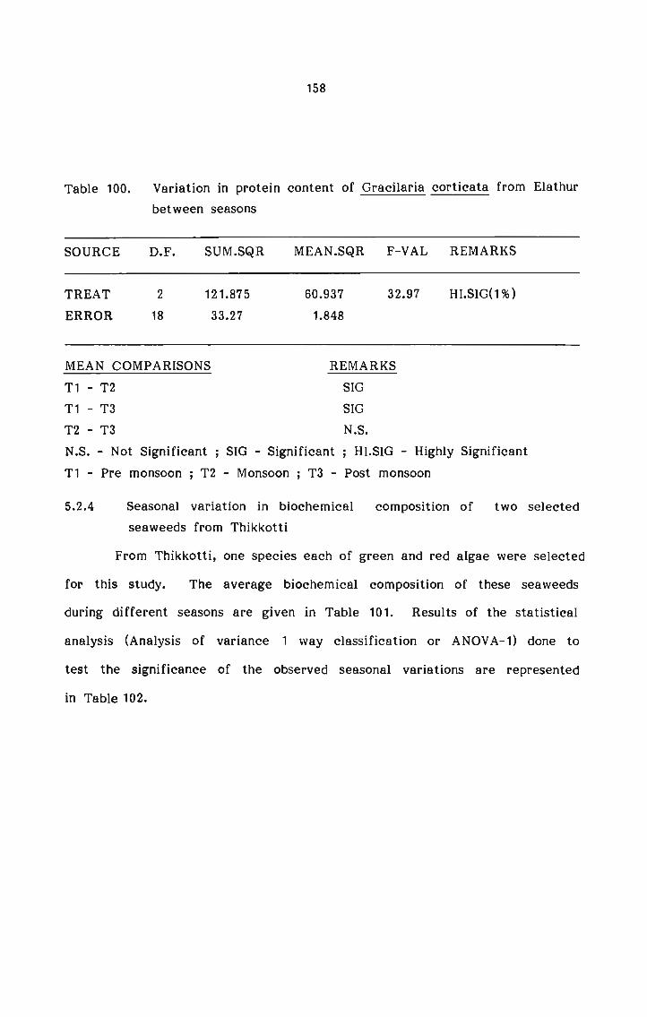
158

Table 100. Variation in protein content of Gracilaria corticata from Elathurbetween seasons



MEAN COMPARISONS REMARKST1 - T2 SIGT1 - T3 SIGT2 - T3 N.S.N.S. - Not Significant ; SIG - Significant ; HI.SIG — Highly SignificantT1 - Pre monsoon ; T2 - Monsoon ; T3 — Post monsoon

5.2.4 Seasonal variation in biochemical composition of two selectedseaweeds from Thikkotti

From Thikkotti, one species each of green and red algae were selected

for this study. The average biochemical composition of these seaweeds

during different seasons are given in Table 101. Results of the statistical

analysis (Analysis of variance 1 way classification or ANOVA-1) done to

test the significance of the observed seasonal variations are represented

in Table 102.

159

:_8:_&_m 2.3: - oa._= N E8_:=m_m sz - .m.z.m.z Q3: o_m._= sS_:o... 2§_2:oo_m.E 93: 05.5 8c_o_._2=:9.. am._2_ao

2.5 o\_a._uEo._._ao 53.5

mfibmca Eofimflfim co woman mv_._mEmm

mm? Mo oEmz

_39_v_E._. E9: mvomaamm ©3028 oz; ._o :o_:moaEoo _mo_EocooE E :o:a_.E> Ecommvm mo oo:ao:E.m_m

flmflmcw Eozmzfim co cmwan

.No— 056%ca: u A N 3w._EEon._ao a O m 5395 u mSmofizoo:2 3.2 23 2.. 8.2 22. 3.; Sea 56 2.2620moEo_._23._mm:8 3.2 3.: 84 8.2 8.2 $6 2...... £2 aI._I§.6o

._ o m A o A. 4 o n_

:oom:oE “mom :oom:oE :oom:oE PE am? we wEmz

mcomwwm u:w._m.C_u 2: .w:._.=6

_Soxv_E.w E0: mummammm _u3o2mm mo :o_:mon_Eoo _mo_EmEooE

oma..w>< .2: Enmp.

160

ANOVA Tables of biochemical constituents that showed significant


Table 103. Variation in protein content of Caulerpa sertularioides fromThikkotti between seasons



MEAN COMPARISONS REMARKST1 - T2 SIGT1 - T3 SIGT2 - T3 N.S.N.S. - Not Significant ; SIG - Significant ; HI.SIG - Highly SignificantT1 - Pre monsoon ; T2 - Monsoon ; T3 - Post monsoon

Table 104. Variation in carbohydrate content of Caulerpa sertularioidesfrom Thikkotti between seasons



MEAN COMPARISONS REMARKST1 - T2 SIGT1 - T3 N.S.T2 - T3 SIGN.S. - Not Significant ; SIG - Significant ; HLSIG - Highly SignificantT1 — Pre monsoon ; T2 - Monsoon ; T3 — Post monsoon

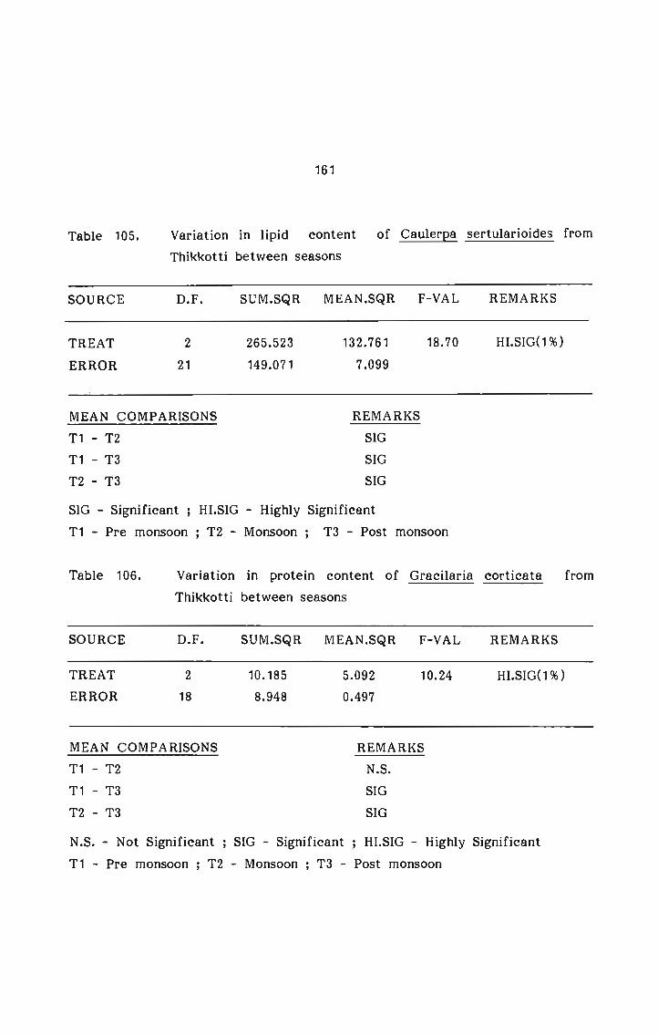
161

Table 105. Variation in lipid content of Caulerpa sertularioides fromThikkotti between seasons



MEAN COMPARISONS REMARKST1 — T2 SIGT1 - T3 SIGT2 - T3 SIGSIG - Significant ; HI.SIG - Highly SignificantT1 - Pre monsoon ; T2 - Monsoon ; T3 - Post monsoon

Table 106. Variation in protein content of Gracilaria corticata fromThikkotti between seasons



MEAN COMPARISONS REMARKST1 - T2 N.S.T1 - T3 SIGT2 - T3 SIGN.S. — Not Significant ; SIG - Significant ; HI.SIG - Highly SignificantT1 - Pre monsoon ; T2 — Monsoon ; T3 - Post monsoon

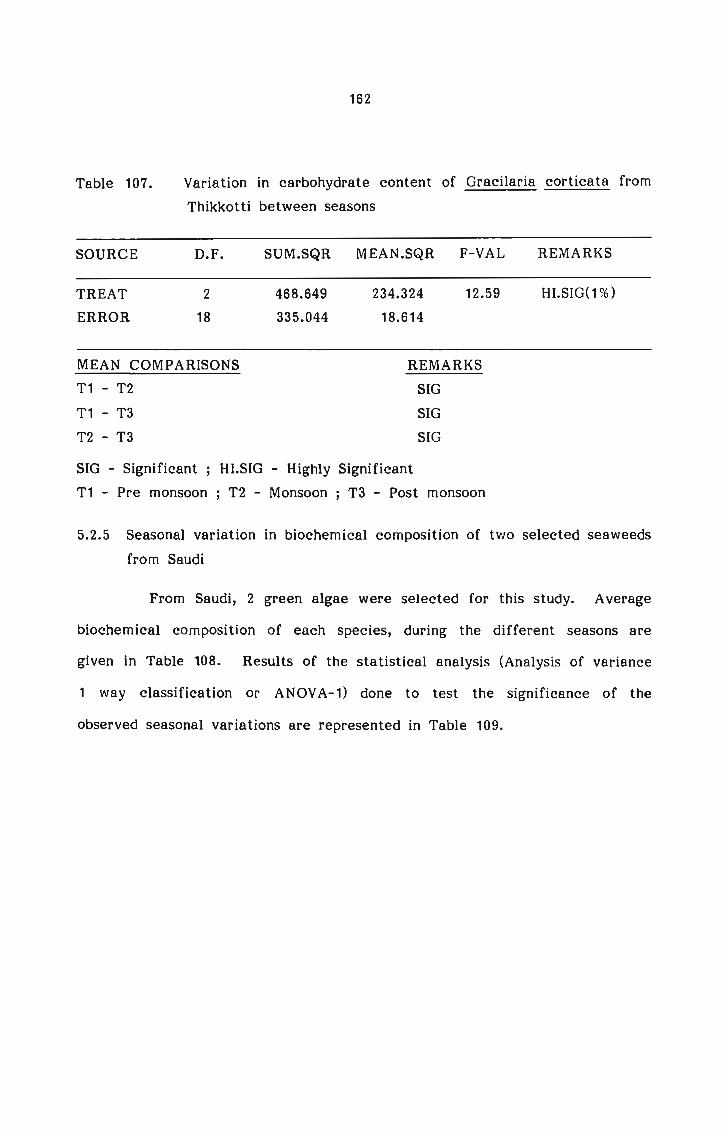
162

Table 107. Variation in carbohydrate content of Gracilaria corticata fromThikkotti between seasons



MEAN COMPARISONS REMARKST1 - T2 SIGT1 - T3 SIGT2 - T3 SIGSIG - Significant ; HI.SIG - Highly SignificantT1 - Pre monsoon ; T2 - Monsoon ; T3 — Post monsoon

5.2.5 Seasonal variation in biochemical composition of two selected seaweedsfrom Saudi

From Saudi, 2 green algae were selected for this study. Average

biochemical composition of each species, during the different seasons are

given in Table 108. Results of the statistical analysis (Analysis of variance

1 way classification or ANOVA-1) done to test the significance of the

observed seasonal variations are represented in Table 109.

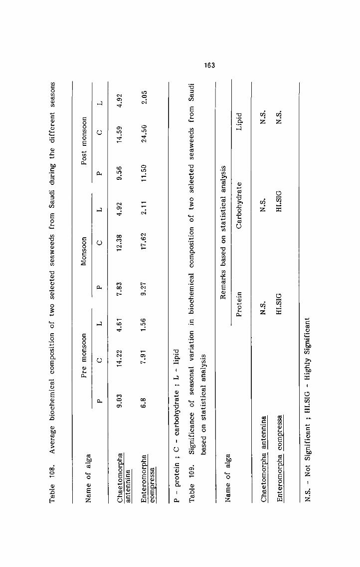
163

E8E&_m 359: - 05.5 _ E8cEm_m “oz - .m.z.m.z O_m._= O_m._= ammw.aEoo wca._oEo..3:m.m.z .m.z .m.z aE::3:w w;m..oE3wm:O

E94 3a._EEoo._wO E3o.E

m_m3w=m Eoflmfimzm co Uwmmn wx._wEwm

am? no vEaz

m_m>_m:a Eozmfifim :o ummwa

Ezwm Eo.c mvmozwmm @3023 oz: go :o_:moaEoo _mo_Em:ooE E :o32.E> Ecomwom mo wo:wocEm_m .2: «SE.

was u A m mumhozzonhao .. O M 530.5 I mammm._mEoo.22 Si 3.: :.~ 3.: S6 3.. S.» we 2m_oE23:mwE::3:w21. 3.3 35 22. 3.5 23 54. «N4: 85 m:m._oE3ww:O

A O m A O m A O m

:oom:oE «mom :oom:o_>_ :oom:oE 95 am? mo mEmz

mcommom Em._ot_c 2: mE.=6

Ezwm EO._.u mummzswmm 03023

025 .«O CO_..ZwOQEOU —wU_E®£UO_D

wwm._m>< .2: mfimm.

164

ANOVA Tables of biochemical constituents that showed significant


Table 110. Variation in protein content of Enteromorpha compressa fromSaudi between seasons



MEAN COMPARISONS REMARKST1 - T2 SIGT1 - T3 SIGT2 - T/ SIGSIG - Significant ; HI.SIG - Highly SignificantT1 - Pre monsoon ; T2 - Monsoon ; T3 - Post monsoon

Table 111. Variation in carbohydrate content of Enteromorpha compressafrom Saudi between seasons




165

5.3 PLACE-WISE VARIATION IN BIOCHEMICAL COMPOSITION (Figs. 27-38)

For this study, 4 species of seaweeds .3 belonging to green algae

and 1 to red algae were selected each of which was collected from more

than one station along the Kerala coast. Average biochemical composition

during the different seasons, for each of these species of seaweeds, are

represented in Tables 112-123. All values were expressed in percentage

dry weight.

Table 112. Station-wise variation in protein content of Ulva fasciata

Seasons StationsMullur Varkala Elathur

Pre monsoon 7.17 8.16 12.15Monsoon 11.85 10.24 14.40Post monsoon 13_23 11.05 14.66

Table 113. Station-wise variation in carbohydrate content of Ulva fasciata


Pre monsoon 29.35 22,33 23,50Monsoon 23.74 22.95 18.50Post monsoon 23.21 24.50 24.00

166

Table 114. Station-wise variation in lipid content of Ulva fasciata


Pre monsoon 1,51 3.91 4.16Monsoon 1.96 2.53 2.20Post monsoon 2.40 3,07 3.16

Table 115. Station-wise variation in protein content of Ulva lactuca


Pre monsoon 4.36 6.53 13.75Monsoon 9.60 8.25 14.10Post monsoon 14_55 3,52 15.36

Table 116. Station-wise variation in carbohydrate content of Ulva Iactuca


Pre monsoon 27.75 31.41 21.50Monsoon 24.40 21.93 19.50Post monsoon 31.00 25.77 28.60

167

Table 117. Station-wise variation in lipid content of Ulva lactuca



Table 118. Station-wise variation in protein content of Chaetomorghaantennina

seasons StationsSaudi Varkala Elathur


Table 119. Station-wise variation in carbohydrate content of Chaetomorphaantennina

Seasons StationsSaudi Varkala Elathur

Pre monsoon 14.22 15.06 6.58Monsoon 12.33 12.84 3_41Post monsoon 14.59 8.70 7.00

168

Table 120. Station-wise variation in lipid content of Chaetomorpha antennina

Seasons StationsSaudi Varkala Elathur


Table 121. Station-wise variation in protein content of Gracilaria corticata

seasons StationsMullur Elathur Thikkotti

Pre monsoon 7.16 6.11 9.51Monsoon 9.81 11.63 8.90Post monsoon 3_43 10.68 7.82

Table 122. Station-wise variation in carbohydrate content of Gracilariacorticata

seasons StationsMullur Elathur Thikkotti

Pre monsoon 25.34 16,73 24_57Monsoon 18.00 18.00 13.00Post monsoon 15.75 23.04 18.75

169

Table 123. Station-wise variation in lipid content of Gracilaria corticata

Seasons StationsMullur Elathur Thikkotti

Pre monsoon 2.62 2_g5 1.30Monsoon 2.47 2.18 1.10Post monsoon 2.09 2.05 1.01Statistical analysis (Analysis of variance 2 way classification

ANOVA-ll) was done to test the significance of place-wise variation in

biochemical composition, and the results are represented in Table 124.

Table 124. Significance of place-wise variation in biochemical compositionbased on statistical analysis

Name of alga Remarks on place-wise variation based onstatistical analysis

Protein Carbohydrate LipidUlva fasciata I-ll.SIG N.S. N.S._Q. lactuca N.S. N.S. N.S.Chaetomorpha N.S. N.S. N.S.antennina

Gracilaria N.S. N.S. HI.SlGcorticata

N.S. - Not Significant ; HI.SIG - Highly Significant

170

Protein content of Ulva fasciata and lipid content of Gracilaria

corticata were found to vary significantly between stations. ANOVA Tables

are given below:

Table 125. Result of statistical analysis done to test the significanceof station-wise variation in protein content of Ulva fasciata


TREAT 2 25.052 12.526 11.75 SIG (5%)REPLIC 2 24.427 12.213 11.45 SIG (5%)ERROR 4 4.265 1.066

TREATMENT MEAN COMPARISONS REMARKST1 - T2 N.S.T1 - T3 SIGT2 — T3 SIGTREAT MT1 10.77T2 9.818T3 13.736REPLICATION MEAN COMPARISONS REMARKSR1 — R2 SIGR1 — R3 SIGR2 - R3 N.S.REPLIC ME_zflR1 9.16R2 12.16R3 12.998N.S. - Not Significant ; SIG — SignificantT1 — Mullur ; T2 - Varkala ; T3 - ElathurR1 - Pre monsoon ; R2 - Monsoon ; R3 — Post monsoon

171

Table 126. Result of statistical analysis done to test the significanceof station—wise variation in lipid content of Gracilariacorticata


TREAT 2 2.602 1.301 62.18 HI.SIG (1%)REPLIC 2 0.122 0.061 2.92 N.S.ERROR 4 0.084 0.021

TREATMENT MEAN COMPARISONS REMARKST1 - T2 N.S.T1 - T3 SIGT2 - T3 SIGN.S. - Not Significant ; SIG — Significant ; HI.SIG - Highly SignificantT1 - Mullur ; T2 — Elathur ; T3 - Thikkotti

WWO. mum.

R9...

mrkzoz

- n.no_- m.

..ON:.::o_m Quit -3

o_9_5> OIIO

5.3.2 Tu Lon

ESum_\..\ V3.3 mo kzmpzooZ_u._.Omn_ z_ zo:<_m<> me; ZO_._.<._.m

3 9ViN33H3d

0mm.

-2-0-co-<--'7

E_.§m_\.« §.S.._O pzmkzoo m:<mo>_._omm<o Z. zo_»<_m<> me; 2925

:.__:_2 I:::o_u O||.Oo_9:o> DID

O.m _ON3ononov

39V.LN3OH3d

0mm. mum. mam.

.2:o_m D|n_

o_9_5> olnlos__=s_ ollo

mm .5

333 E 3::.._O SE28 o_n__._ Z_ zo_E_m<> mm_2, zo_:Em

39ViN33H3d

one...

WWW. WWW.

mzkzoz

<2..__.ozom

I

F

:::.._m Io_o.:o> OIO3__:s_ TD

vfibkbvfi 3:: .._o pzmpzoozmeoma z_ zo:<E<> mm;> zO_._.<._.w

0ID:0 ON N39ViN33U3d

O('0

mmm; mmm.

mzhzoz

u _., m. J.

omm _

O—

242...

..

.532.‘ m,__;._..

.6393 $33no kzmizoo m:Eo>:omm<o Z. zo_»<_m<> mm_>> ZO_._.<.rm.:::.._n._ Io_9_.o> 0'0:..__DE 0'0

LInN

L

0ID0 OM N39ViN33H3d

mm

OWN. mmm. WWW.

mxkzoz

1 o z 0 m < a 3 Z < E m a 0 Z m

1 . . . . . . 4 4 . . . . . _ . .

:_£o_m UIIUo_e_5> o.||.o

5.35. To

an .5

3:33 §.S.._O pzupzoo o_n:4 z_ zoF<_m<> mmi zofifim

NV I039ViN33H3d

0mm. mam. mam.

MIHZOE

:._L_f3.:_.:<z:m_,_Z.l,_‘__.,.<_‘,.Z.:

3£a_m Isnow oIIoo_9_:.> alum

mm?

Sszzmuzw vtmmosotvru no ..zH.:zooz_E.oE z_ zo:<_m<> was 2925

OInON

IO(‘V

0r0

39ViN33H3d

:E_o_m I

InN

'39VJ.N33H3d

o_ofo> OIOBaum DID

woo:

3<§<E\§ 3.E..<o:Em§uno 5528 mfimoiommqo z_ zo:<E<> um;> 2925

0IO

0mm. mam. w.wm_

‘W5

_.:am U|U o

555 9I|o . ..

o_9_a> To _.

<2=<2m:2< VIQQOEQKMQIUn.O ._.zm._.zOo oi: Z. zO_._.<_m<> me; 2925

moor.

39Vl.N33H3d

omm.

mam.

on .o_..,_

_:e:_.: olo:_£on._ I5.3.2 0'0

.\.~<UCt0b _\E_\.:.uSw6.._o 5528 255$ z_ zo_E_m<> mm_; ZO_._.<._.m

'0 ON N39V.LN33U3d

0F0

0mm. mam:

E cotton 3%? dusmu..._O hzmpzoo u»<mo>:omm<o Z_ zo:<_m<> m_m_; ZO:.<._.w

_:9_.__.: 0'0.:=:2 OIIO.3:oE OILO

5.0:

0LOL0 ON N39\1.LN3383d

O('0mm

omm_

mmm;

_:9_.__.: I:::_._m_ I5__..s_ ¢:|lo

mm .9...

Szétmou Smqduqmmn_O SE28 ea... z_ zo:<_m<> mmi zo:<.5

V I039V.LN30t|3d

ID(0

5.4. PARAMETER! IIOWING CORRELATION WITH BIOCHEMICAL CONSTITUTION or SEAWEEDS

Table I2? Parameters sratnnng correlation with lion.-hernical conttitution of seaweeds

NI\Ml1(l' PI\iU\Hl.‘|'i)t TYPIJ 0' (IJILRHATDN wuummzn TVPI OI‘ (O1llt.H|A'|'DN P/t|t.AME|'l-IR TYPE OF ("ERR.ElA‘lI)NMAM ANIJ SKEW: (Oit|tI]A'TI')N (1Jf}'I-YT!-III‘ SIGIING C1Il‘t'*'.|.A'lDN (DI-}'|"l1lZNI' SDWIMZ (INt.Il}JA'IK)N (DI-J'l'Il}N'|'STATIN OI‘ (DRIUIATKN CIBIJIVIJI (DRREATIN CIEJWI-J) (DRRILATOJ CI'E'IN\/Hi(‘l.l..|J'l'l@ Wml MIN Wmi UPIIJ|'lN7l'H|N CAR.Kl'iYDiU\1'EQaulere Salinity Positive 0.543 Surface Pouitlve 0.4l3 Protein Negative - 0.020£l Nitrate Pulllve 0.550 ::;"m"‘I'HlKKO1'I'l Phoaphat Negativa -0.562 Carbohy- Poaltlve 0.535

lllieate Negative -0.500 ‘"I'Gran.-ilaria Atmospheric Negative - 0.409 Dlnolved Ptmtive 0.62lcarnal. temperature otygen

SurfaceELATHUII Water Negative - 0.576 Salinity Positive 0.491 - - temper-ture

(_Zhaetor_n§t£ Salinity Positive 0.414 Salinity Positive 0.555 Monthly Positive 0-400Silicate Negative - 0.42l Protein Piritive 0.650 'SAUDI Silicate Positive 0.501Ulvafaseiata - - - Thoaphate Negative -0.630 - - VARNALA

l_J.la¢.-tuea MonthlyIeaveed Punitive 0.417 Atmospheric Positive 0.492VAIIIUI-A density . . temperaturePhosphate Negative - 0.505 Salinity Negative - 0.732grueloilij Atmospheric Negative - 0.54l Atmcapheric Puitive 0.4llImam". temperature temperatureVMIKALA Surface Negative -0.6l0 Phoaphate Pcsltlve 0.414 -

Watertemperature Silicate Positive 0.499Protein Negative -0.151

Ulva Nitrate Puitive 0.516 Protein Nqative -0.842 Nitrate Positive 0.520taaelataMULLUI

Q. laetuea Nitrate Punitive 0.460 Protein Positive ant,“ - —IIULLUN Silicate Negative - 0.530gaulei Monthly5 Ieaueed Positive 0.410 Atnmhcle Positive 0.553 Nitrate Nqative - 0.67402'5"! temperature

llllcate Poaitive 0.512 Carbohy- Positive 0.506drate

Li a Iurfuoelm VII" Negative . n.sou . . . cm». Negative . 0.'Il6MULLUII ""‘P"'“"' hydrateNitrate Positive 0.540

‘nu,..:,',,,,,,._ 5"-we Ne:-me - 0.420 . . - Surface Paitlve 0.5::“UI-I-UI‘ I"e.rI:p:ratureSurface Negative - 0.405 Protein Nqative - 0.501 Atmospheric Nqative - 0.393"'9' temperaturelemwralure

Phosphate Positive 0.473Carbo- _.war". Pmitive 0.4l0Sagnaum __ 7' M" ' rhasphote Nqative - 0.591 Surface Punitive 0.43!-L rater"L-LL”; temperature

- Silicate Negative - 0.440 Nitrate Nqalive - 0.497°‘"’°' Positive 0..-sohydrate

6. DISCUSSION

6.1 ECOLOGY OF SEAWEEDS

In the present study, 52 species of seaweeds, 20 belonging to

Chlorophyta, 10 to Phieophyta and 22 to Rhodophyta were recorded from

Kerala coast. Anon (1981) reported the occurrence of 17 species of seaweeds

from Kerala, 5 belonging to Chlorophyta, 8 to Phieophyta and 4 to Rhodophyta.

Balakrishnan Nair Q fl (1982) reported 44 species of seaweeds, from the

south-west coast of India, 17 belonging to Chlorophyta, 6 to Phieophyta

and 21 to Rhodophyta. Out of these,8 species were recorded exclusively

from Kanyakumari (Tamil Nadu) and the rest from Kerala. Sobha and

Balakrishnan Nair (1983) recorded the occurrence of 34 species of algae

from south-west coast of India, out of which 27 species were collected

by the authors from Cape Comorin, and the rest from Kerala. Chennubhotla

e_t_££ (1983) gave a list of 34 species of seaweeds collected from the inter

tidal and subtidal regions of Kerala coast. Out of these, 24 species were

recorded in the present study also. Sobha and Balakrishnan Nair (1985)

reported the occurrence of 44 species of algae from Kerala, including 17

species collected from Kanyakumari. Out of the species recorded by the

above authors, 22 species were recorded in the present study also.

Chennubhotla e_t a_l (1986) recorded 35 species of seaweeds from Kerala,

out of which 30 species were recorded in the present study also. Balakrishnan

Nair Q 9_1(1986) recorded 101 species of seaweeds from Kerala coast.

But their study included stations like Muttom and Cape Comorin in Tamil

Nadu and Mahe in Pondicherry, and the authors have not indicated the

exact place of collection of each species of seaweed. and a list of seaweeds

174

from Kerala, including the above mentioned stations is given. Cape Comorin

is a place noted for its distinctive marine algal flora, which for its diversity

and luxuriance is noteworthy (Sreenivasan, 1969). Inclusion of this station

in all the studies relating to marine algal flora of Kerala by the authors,

have created a lot of confusion regarding the species of seaweeds recorded

exclusively from Kerala.

Along the Kerala coast, in the present study, Rhodophycean algae

showed maximum diversity with 22 species, followed by Chlorophyceae

with 20 species. Phiaophycean algae were comparatively less along the

Kerala coast with only 10 species. Agadi and Untawale (1978) reported

51 species of marine algae from Goa, out of which 19 belonged to

Rhodophyta, 15 to Phfiophyta, 13 to Chlorophyta and 4 to Cyanophyta.

Diversity-wise Rhodophycean algae were more in Goa, as was observed

in the present study. Number of green and red algae recorded from Goa,

was less than that of Kerala but brown algae were more in Goa.

Murthy e_t a_l (1978) recorded more of Rhodophycean algae along

Gujarat coast. Gopinathan and Panigrahy (1983) recorded 55 species of

marine algae from Andaman and Nicobar islands, out of which 16 belonged

to Chlorophyta, 17 to Ph?ophyta and 22 to Rhodophyta. Here also diversity

wise red algae outnumbered other divisions of algae. Number of green

algal species recorded from these islands was less than that in Kerala,

but brown algae were more in number. Kaliaperumal and Pandian (1984)

studied the distribution pattern of marine algae in 6 localities of Tamil

Nadu, and found that in all the stations studied, red algae were more in

number. The marine macrophytes of Minicoy Atoll were studied by Untawale

175

and Jagtap (1984). Out of the 37 species of algae reported by them, 10

belonged to Chlorophyta, 5 to Phgfieophyta 19 to Rhodophyta and 3 to Cyano

phyta. Number of species of all divisions of algae from Minicoy, reported

by them was less than that recorded from Kerala coast in the present

study. Subba Rao _e_t_ a_l (1985) recorded 65 species of marine algae from

Andhra coast, out of which 23 belonged to Chlorophyta, 7 to Phaiaophyta,

34 to Rhodophyta and 1 to Cyanophyta. The number of green and red

algae from Andhra was more than that of Kerala but the number of brown

algae was less. Agadi (1985) recorded 42 species of algae, 16 each belonging

to Chlorophyta and Rhodophyta and 10 to Plireophyta, from Karnataka coast.

Though the red and green algae were lesser in number than in Kerala,

the number of brown algae was the same in both places. Jagtap (1985)

recorded 64 species of marine algae from Andaman islands, 26 species

belonged to Rhodophyta 21 to Chlorophyta, 14 to Ph:eophyta and 3 to

Cyanophyta. Number of algae belonging to each division was lesser in

Kerala compared to Andaman Islands as reported by him. Kaliaperumal

e_t Q (1989) studied the seaweed resources of 12 islands of Lakshadweep.

They recorded 43 species of Chlorophyceae, 14 species of Phféophyceae

and 54 species of Rhodophyceae. In all islands studied by them, maximum

diversity was found in Rhodophycean algae, and minimum in Phiaophycean

algae, as was observed in Kerala.

Thus almost throughout the entire coast of India, Rhodophyta out

numbered all other divisions in terms of diversity and Phajeophycean algae

were comparatively less. Misra (1965) suggested that tropical ecological

176

conditions, especially extremely high range of temperature and long periods

of severe insolation are responsible for the absence of many brown algae,

which occur in the temperate regions of the world, from Indian coasts.

Red algae on the other hand may be more tolerant to the tropical environ

mental conditions.

6.1.1 Environmental factors controlling species composition, distributionand density of seaweeds

Species composition, diversity and density of seaweeds varied

significantly from station to station in the present study. Thikkotti showed

the maximum species diversity with 37 species of seaweeds, followed by

Mullur with 33 species. Varkala recorded 22 species, Elathur 21 species

and Saudi 9 species. Mullur recorded the highest density of 3971.25 gm

of seaweeds/m2 (wet weight) followed by Varkala with 2047.50 gm/m2.

Elathur recorded 1832.29 gm/m2, Thikkotti 1408.13 gm/m2 and Saudi

1387.50 gm/m2. The station which showed the highest diversity of seaweeds

did not thus show the highest density. Therefore it can be said that the

factors controlling the occurrence and distribution of a species of seaweed

need not necessarily be conclusive for its further growth and development.

Distribution and growth of seaweeds is therefore a combined or synergetic

effect of a number of environmental and other biotic factors, out of which

some factors play major roles, while others minor roles.

In order to get a clear picture of the cause of disparity observed

between stations, in species composition, diversity and density of seaweeds,

the environmental peculiarities observed at each station and its possible

effect on the above mentioned aspects of seaweeds are briefed below.

177

Krishnamurthy (1965) and Krishnamurthy and Subbaramiah (1970)

described the importance of shore types in the zonation of Indian marine

algae. According to them sandy shores are bereft of algal vegetation,

because of the absence of firm substratum for attachment, while rocky

shores harbour a good amount of algae. A similar observation was made

along the Kerala coast during the present study. The Central zone of

Kerala from Kollam in the South to Kozhikode in the North is sandy with

complete absence of rocks and boulders in the sea, unlike the other parts

of Kerala coast. The representative station in this zone—Saudi-differed

from all other stations studied, mainly in this regard. In this context,

it may be noted that, in the present study, Saudi recorded the lowest density

and diversity of seaweeds. Moreover no Phieophycean alga Was recorded

from Saudi. Mullur in the South zone quite unlike the other stations had

a vast expanse of natural rocks and boulders extending several metres into

the sea and submerged at varying depths, a factor that might have favourably

influenced the distribution and density of seaweeds in this area. This station

recorded the highest seaweed density, good diversity and highest number

of Phféophycean algae. Moreover most of the seaweeds from this station

showed very high frequency of occurrence. All these can well be attributed

to the vast expanse of rocks and boulders in this area, which serves as

a suitable substratum for settlement of seaweed spores and its development.

Varkala, the second station in South zone recorded a lower density and

diversity of seaweeds compared to Mullur. This disparity can mainly be

due to the lesser number of natural rocks and boulders in the area. Moreover

178

rocks were observed only upto a distance of 2 m into the sea in this area,

thus greatly reducing the width of the seaweed belt. Elathur in Northzone was also bestowed with outcrops of natural rocks submerged at varying

depths upto a distance of 5 m into the sea from the shore. Thikkotti

had a sandy beach with numerous sand covered rocks extending upto a

distance of 4 m from the shore into the sea. Unlike Saudi, Thikkotti showed

the occurrence of many psammophytic species of seaweeds like Caulerpa.

From the above, it is clear that absence of suitable substratum

was primarily responsible for delimiting the growth of many varieties of

algae, especially in the Central zone of Kerala. substratum is an essential

pre-requisite for distribution and growth of algae and the disparity observed

between stations in species composition, density and diversity is mainly

due to the disparity in availability of substratum.

General information on the effects of sand on marine communities

are given by Chapman (1943, 1955), Stephenson (1943) and Lewis (1964).

Srinivasan (1969), reported that sandy beaches harbour very little or few

algal forms, while hard substratum supports innumerable variety of algae.

Untawale and Dhargalkar (1975) observed that along Goa coast, seaweed

growth occurs mostly along rocky shores while sandy shores are devoid

of macrophytes. They suggested that constant accretion and erosion were

responsible for the absence of algae along sandy beaches. Daly and Mathieson

(1977) suggested that sandy beaches exhibit reduced populations of seaweeds

because of extensive sand abrasion, reduced light levels and

179

lack of stable substrate. Subbaramiah _<1a_l (1977) observed that the distri

bution and growth of marine algae in Pamban area is mainly controlled

by availability of substratum. Agadi and Untawale (1978) suggested that

along Goa coast an important factor for algal growth is the nature of

substratum. Agadi (1985) noted that along Karnataka coast, sandy areas

were devoid of algal growth. Shunula (1985) observed that sandy beaches

were devoid of algal vegetation in the five shores of Zanzibar, studied

by him. Trono Jr. (1988) observed that different types of substratum

influence the local distribution of seaweed species.

Temperature is another major factor that was observed to play an

important role in controlling the distribution, diversity and density of

seaweeds in the present study. Statistical analysis revealed that there

was significant variation in the surface water temperatures between stations.

Variation in atmospheric temperature between stations though not found

to be statistically significant, its biological significance cannot be ruled

out. In the present study, Saudi recorded the highest atmospheric and surface

water temperature. Densities of two species of algae, Ulva fasciata and

E. lactuca showed a negative correlation with temperature. These two

algae were found to grow in all the stations studied except Saudi. Nienhius

(1971) observed the explosive development of Enteromorpha spp. at higher

temperatures. This alga was observed to be growing abundantly in Saudi.

Therefore it can well be assumed that temperature plays an important

role in controlling the algal distribution. Severe insolation may be considered

an important factor in the absence of brown algal species at Saudi. In

180

the present study, Mullur recorded the lowest atmospheric and surface

water temperature which might have favourably influenced the seaweed

growth in the area. Varkala recorded higher atmospheric and surface water

temperature than Mullur and here the effect of insolation also was observed

to be more. This is because, at Varkala, rocks were submerged only upto

a depth of 0.75 m in the sea, unlike that in Mullur. This factor might

have played an important role in the absence of many species of seaweeds

recorded at Mullur, from Varkala. Krishnamurthy (1965) observed that

in tropical intertidal shores, only a few algae grow due to intense insolation

and strong light which makes the coast uninhabitable to algae not adapted

to withstand dessication. Chapman (1978) observed that sea temperatures

affect biogeographic distribution and sets limits to many species of seaweeds.

Trono Jr. (1988), suggested that the local distribution of seaweeds in inter

tidal areas and tide pools are influenced by temperature and that very

high temperatures often excludes many algal species.

A third factor that was found to control the occurrence and density

of seaweeds in the present study was salinity. Among all the stations

studied, lowest salinity was recorded at Saudi and this area showed wide

fluctuations in salinity regimes. During monsoon, salinities as low as 17

ppt and 18 ppt were recorded at Saudi. This might have been a primary

factor that restricted the density and distribution of seaweeds at Saudi.

This is further confirmed by the fact that Mullur with high density and

diversity of seaweeds recorded the highest mean salinity. Elathur also

recorded comparatively lower salinity and here also salinities fluctuated

181

between 21 ppt during monsoon to 36.6 ppt during post monsoon. This

might have controlled the seaweed distribution and growth in the area,

inspite of the fact that enough substratum for seaweed growth were available

at Elathur. Various floristic studies along salinity gradients in estuaries

and lagoons (Doty and New house, 1954; Conover, 1964; Munda, 1978;

Coutinho and Seelinger, 1984) have documented a reduction in species

diversity with increasing dilution and concentration of sea water and have

postulated the halotolerance of marine algae based on their distribution.

Marine red algae as a whole are considered to be sensitive to mesohaline

conditions (5-18%. ) as relatively few representatives are recorded from

salinities below 15%: (Munda 1978; Coutinho and Seelinger 1984). According

to Munda (1978) salinity along with substrate configuration is the major

factor responsible for changes in algal growth. Durairatnam and Reghu—

nathamuthaliar (1973) suggested that water temperature had no effect on

algal growth whereas salinity affected the growth of algae. Chapman (1978)

suggested that salinity factor is very important in estuaries where red

and brown algae tend to disappear. Bird and Mc.Lachlan (1986) studied

the effect of salinity on the distribution of several species of Gracilaria.

Euryhalinity of most isolates suggested that salinity is not a critical factor

in determining its distribution. But maximum growth occurred at salinities

of the natural environment. Umamaheswara Rao (1987) observed that as

salinity decreased there was a reduction in members of red algae and green

algae became more abundant. Gavino Trono Jr. (1988) observed that there

is a low diversity of seaweeds in habitats with highly fluctuating salinity

regimes.

182

In the present study, the dissolved oxygen content was found to

vary significantly between stations. Elathur recorded the lowest dissolved

oxygen content. Saudi and Thikkotti recorded almost the same dissolved

oxygen content. Elathur recorded a higher density of seaweeds than both

Saudi and Thikkotti and a greater species diversity than Saudi. Densities

of many species of algae were found to have a positive correlation with

dissolved oxygen content of ambient waters. Therefore it can be said

that eventhough dissolved oxygen content of the waters is not a critical

factor in controlling the marine algal density and diversity, it does favourably

influence the seaweed growth when available in good quantities. This may

be one of the reasons for the good algal growth at Mullur, which recorded

the highest dissolved oxygen content in the present study. Gaur Q Q

(1982) observed a positive correlation between phytomass of fig lactuca

and dissolved oxygen content as was observed in the present study. Gavino

Trono Jr. (1988) observed that dissolved oxygen content never becomes

a limiting factor for the growth and development of seaweed communities.

This observation was similar to the one made in the present study.

Rodhe (1948) and Blinks (1951) have cited the availability of nutrients

as an important factor in governing the distribution of algae and that

phosphorous and nitrogen are often limiting. In the present study, Mullur

with comparatively lower concentrations of nutrients recorded high density

and diversity of seaweeds. Saudi which had the highest concentration of

nutrients, recorded low density and diversity of seaweeds. Densities of

some species of algae were found to show correlations (positive or negative)

183

with one or more of the nutrients in the present study. Therefore it can

be said that the optimum amount and type of nutrients required for proper

growth and development is specific for each species. When required nutrients

are available in the optimum quantities in the station of growth, the species

thrive well. But like dissolved oxygen content, nutrients also do not play

a critical role in controlling seaweed density and diversity. Murthy

e_t Q (1978) observed that nutrients are not limiting for intertidal algae

because of remineralisation from dead forms coupled with efficient mixing

of waters. Agadi and Untawale (1978) suggested that nutrients promote

growth of algae, but unlike temperature, tides etc. are not controlling

factors in the distribution of algae. According to them seawater in the

coastal areas are rich in nutrients needed for algal growth. Chapman (1978)

suggested that nutrient variations in seawater are mainly of concern in

development of plankton but not an important factor in controlling seaweed

vegetation. Gaur e_t_ Q (1982) suggested that the availability of nutrients

in seawater was not related to phytomass production of E lactuca. Inger

Wallentinus (1983) conducted in-situ experiments with different combinations

of annual and perennial seaweeds, simultaneously exposed to varying ambient

conditions. He demonstrated that while- nutrient uptake by annual macro

algae were much higher than that of perennials and strongly correlated

to nutrient concentrations of water, their productivity did not increase

to the same extent and was less dependent on ambient nutrient concentra

tions.

184

Another major factor that appeared to influence seaweed density

and diversity, in the present study was turbidity of the ambient waters.

At Elathur, the water was observed to be turbid throughout the year

especially during monsoon due to the influx of fresh water. This was found

to adversely affect the light penetration to the deeper waters in this area.

Dawson (1966) suggested that transparency of the waters largely determines

the thickness of the productive zone. Srinivasan, (1969) described the

clearness of seawater as an important factor in influencing the growth

of seaweeds. According to him many seaweeds are susceptible to turbidity

and pollution of seawater and only a few marine algae tolerate such environ

ments. This may be one of the major reasons why Elathur bestowed with

an abundance of natural substratum did not show as much seaweed growth

and diversity as Mullur. Chapman (1978) observed that a combination of

light intensity and clarity of water will determine the maximum depth

to which seaweeds can descend. According to him for every sublittoral

alga there must be a minimum light intensity below which there is no

growth.

In the present study it was observed that Varkala and Saudi were

subjected to heavy breakers and high swells especially during monsoon,

which often results in sea erosion in this area. Thus wave action might

have adversely affected the growth of algae in this area. Srinivasan (1969)

suggested that exposed rocks subjected to heavy breakers and swells, harbour

algae with strong hold fasts. In the present study also species like

185

Chaetomorpha antennina, Grateloupia filicina and Q. lithophila with strong

holdfasts were found to grow on rocks exposed to heavy breakers and swells.

Arudpragasam (1970) observed that at Galle Buck in Sri Lanka the variation

in species composition was related to wave action. Chapman and Chapman

(1975) suggested that tidal currents affect the growth of plants and presence

or absence of seaweed species. According to them wave tolerant species

have strong holdfasts and higher tensile strength of thalli and rapid attach

ment of swarmers to rocky substrate. Chapman (1978) suggested that wave

action is essentially a presence or absence factor for algal vegetation in

an area. According to him, it can also be a modifying factor as big waves

elevate the height of seaweed communities along the littoral zone. Agadi

and Untawale (1978) suggested that both tidal currents and waves affect

the growth of seaweeds. Agadi (1983) observed that along Anjuna coast,

Goa, during mid February there is tremendous increase in wind direction

and speed making coastal waters turbulent resulting in uprooting and removal

of algal crop. Trono Jr. (1988) observed that big waves mechanically remove

significant amounts of seaweed stock as illustrated by the tremendous

amounts of drift weeds that accumulate on the shore after a storm.

Morphological changes in the topography of Varkala beach was noticed

during the present study. Periodically, the artificial sea wall made of

granite on which the seaweeds grew were completely covered by sand.

Similar observations were made by Umamaheswara Rao and Sreeramulu

(1964) at Vishakapatnam coast. Daly and Mathieson (1977) studied the

sand movement and benthic intertidal organisms at New Hampshire, U.S.A.

186

According to them the lower intertidal zone was dominated by opportunistic

annuals like Enteromorpha spp. and psammophytic seaweeds. Similar

observation was made at Varkala during the present study. According to

the authors the limited species diversity of seaweeds at the study area

is attributable to unstable environmental conditions and limited number

of habitats. Therefore the seasonal sand movement observed at Varkala

can be considered a major factor that delimited seaweed density and diversity

in the area. Krishnamurthy and Balasundaram (1990) reported the covering

and uncovering of rocks of the intertidal region by sand along Tiruchendur

shore. According to them this is a regular feature in various places of

South India. Murthy and Varadhachari (1980) observed morphological changes

at Valiathura beach, near Trivandrum. They attributed it to turbulent

diffusion, advection etc. related to wave action. This may hold true with

Varkala beach also.

Misra (1959) described temperature, tidal depth, submergence,

emergence, salinity, pH and biotic factors as responsible for algal growth.

Jones (1959) found that currents enhanced the growth of Gracilaria verrucosa

by exposing more of the thallus to light. Conover (1968) recorded

differential standing crops of seaweeds under varying current regimes and

stated that the effects of currents are to produce faster uptake and diffusion

of dissolved substances. Prescott (1969) suggested that the growth and

distribution of marine algal flora depends on topography, geological features,

physico-chemical characters of water and other biological factors. Srinivasan

(1969) described nature of substratum, effect of tides, surf and wave action,

’ 187clearness of water, biotic and seasonal changes as important factors affecting

seaweed growth. Doty (1971b) observed that the water motion is beneficial

to the growth of algae as it enhances better absorption of nutrients. Chapman

(1978) described various factors like photoperiod, tides, submergence exposure,

water loss, wave action, tidal currents, substrate, humidity, temperature,

pressure, light and other chemical and biological factors as influencing

the algal vegetation. Trono Jr. (1988) suggested that quality and intensity

of light changes, as it penetrates the water column, which in turn affects

the distribution of various species. According to him, water movement

caused by waves and currents aerates the water and helps in nutrient

transport, prevents water temperature from rising and favours good light

penetration. Water depth also, according to him, is important in influencing

the abundance and distribution of seaweeds. Thomas and Subbaramaih (1990)

observed that Sargassum wightii had a shading effect on the growth ofother seaweeds.

From the above, it is clear that a combination of environmental

factors operating at each station together with the specific preferences

of each species of algae act and counteract to determine the algal

composition,diversity and density of any given area.

6.1.2 Seasonal changes in species composition, distribution and densityof seaweeds

Misra (1965) observed that corresponding with the changes brought

about by tropical monsoonic and temperate conditions marine algal vegetation

188

undergoes marked seasonal successions. In the present study also marked

seasonal changes in algal distribution, species composition, number of species,

dominant species, and density of each species were observed. Balasundaram

(1985) made similar observation on the Tiruchendur shore. Along Kerala

coast, post monsoon season (September-December) recorded the highest

seaweed density, followed by pre-monsoon. Brown algal density was maximum

during pre monsoon and red algal density during post monsoon. Both red

and brown algal densities were minimum during monsoon. Misra (1965)

observed that October-November period marked by the end of South—west

monsoon, constitutes the regeneration period of all types of algae, and

the earliest to grow is Chlorophyceae. Growth of species of Dictyota,

Padina, Spathoglossum and Sargassum occur. Occasionally such growths

show reproductive structures on the thalli. The progress of vegetative

phase becomes very active and marked, during late November-January.

January was observed by him to be the climatic climax for algal growth

on the west coast littoral regions. Dictyotales and Fucales maintain their

growth through February and May and according to him can reasonably

be called as reproductive period. In the succeeding monsoonic period

beginning in June and extending upto September, all algal growth declines

and ultimately comes to an end. Similar observations were made along

the Kerala coast during the present study. High densities of red and brown

algae observed during post and pre monsoon seasons may be corresponding

to the growth and reproductive phases of these algae which are reported

to occur during late post monsoon and pre monsoon.

189.

Sreenivasan (1969) observed that seasons had marked effect on the

growth of several species of seaweeds, particularly those flourishing on

the upper limits of littoral belts. According to him the cool winter months

of December and January support a climax of littoral algal vegetation.

Gopalakrishnan (1970) observed that red and brown algae appear in large

quantities during post monsoon and last till the end of April ie, pre monsoon.

This observation was similar to the one obtained in the present study.

Agadi and Untawale (1978) observed that along Goa coast, the period from

November to March was the best season for algal growth. Similar

observation was made along the Kerala coast during the present study.

Agadi (1983) observed that along the Anjuna coast of Goa, maximum biomass

was recorded during December-January which gradually decreased thereafter.

From March to August algal growth was negligible. According to him more

number of species were observed during December-January when water

temperature is low and wave action mild. Thereafter the number of algal

species shows a gradual decrease during summer when temperature is high

and nutrients in water low. Gavino Trono Jr. and Teresita Buchan (1987)

studied the seasonality in biomass of Acanthophora spicifera in Bacoor

Bay, Philippines. According to them the biomass production was high during

colder, calmer months of November-January and low during the rest of

the year. Along Kerala coast also, this alga was collected as cast upweed from the Thikkotti beach during the period from November to January.

Balakrishnan Nair fl a_l (1990) surveyed the occurrence, distribution and

relative abundance of brown algae at four representative stations along

190

South-west coast of India. They observed that species composition of brown

algae varied with stations, as was observed along Kerala coast during the

present study. They also observed that brown algal density increased during

monsoon. But this observation was quite contrary to the one obtained

in the present study, where brown algal density decreased during monsoon.

Sampathkumar Q a_l (1990) observed that in Pudumadam and Tuticorin the

biomass of Ph?éophycean algae was more during post-monsoon than monsoon

as was observed in the present investigation. In the present study, there

was a marked fall in brown and red algal densities during monsoon. The

heavy rains during monsoon, often results in severe wave action and tidal

currents. During this period many delicate seaweeds get washed off. Only

those species with strong holdfasts survive the turbulence of the sea. This

is one of the factors responsible for the reduction of brown and red algal

species during monsoon. Transparency or clarity of water is another

important factor influencing the density of seaweeds. Agadi and Untawale

(1978) suggested that transparency value of 3.3 m observed during post

monsoon favoured the growth of seaweeds at Goa and the value of

0.2 m observed during monsoon had an adverse effect on the growth. As

discussed earlier turbidity of the waters hampers light penetration. This

in turn will affect the density of the seaweeds especially those of the

deeper waters. These areas are usually occupied by red and brown algae,

and hence the seasonal reduction in densities of these two divisions of

algae during monsoon.

191

Density of green algae was observed to be maximum during monsoon

in the present study. Densities of many species of green algae showed

a negative correlation with temperature. It was also observed that during

monsoon, the atmospheric temperature, surface water temperature and

salinity decreased and nutrient concentrations increased due to upwelling.

Therefore it can be said that the low atmospheric temperature, surface

water temperature and salinity and the high nutrient concentrations in

the ambient waters observed during monsoon, favoured the growth of green

algae. Shunula (1983) studied the biomass trends of Elv_a _fasciata in

Dar-es-salaam, Tanzania. He observed that the standing crop of E. fasciata_

was highest during cool months and lowest during hot months due to

insolation, heating, evaporation and dessication. Salinity around the thallus

increases during hot season leading to plasmolysis and death of alga. Similar

observation was made by Lawson (1957) on the west coast of Ghana. This

might be the case along the Kerala coast also during pre and post monsoon

periods with regard to green algae. Balakrishnan Nair _e_t a_l (1990) studied

the occurrence, distribution, growth and abundance of green algae from

South-west coast of India. According to them the maximum of green algae

was observed during monsoon, due to low temperature, low salinity, low

dessication and increased nutrient concentrations in ambient waters. This

confirms the observation made in the present study.

Along the Kerala coast seasonal variation was observed in the environ

mental factors studied like atmospheric and surface water temperature,

192

salinity, dissolved oxygen content and concentration of nutrients like

phosphate, nitrate and silicate in the ambient waters. Seasonal variation

in surface water temperature, phosphate and silicate contents were very

significant statistically. Densities of several species of seaweeds were

found to be correlated with one or more of these parameters in the present

study. Therefore it can be said that monthly/seasonal variation in the

environmental parameters is one of the factors responsible for the monthly/

seasonal variation in seaweed densities. But the way these parameters

affect the seaweed density varies with algal division, species etc.

Several authors have studied the seasonal variation in seaweed densities

and have explained it in different ways. Lawson (1957) observed a correlation

between the seasonal changes in the growth of Hypnea musciformis and

seasonal changes in tides at Ghana. Similar observations was made by

Richardson (1969) for the same species at Trinidad coast. Rama Rao (1972)

observed that seasonal changes in lowest lower low water (LLLW) along

with parameters like exposure to air and temperature control the seasonal

changes in density, growth and upper limit of Hypnea musciformis along

the Indian coast. Prasanna Varma (1959) suggested that in Palk Bay, maximum

growth and vegetation occurred during months of low salinity, and rhythmic

fluctuations in total nitrogen seems to correspond with periodic vegetative

and reproductive phases of algae. According to him consideration of

temperature as a contributory factor has limited scope. Doty (1971a)

193

observed that in tropical non—monsoonal areas like Hawaii, random effects

of storm is the most influential factor regulating the size of marine algal

crop, and seasonal factors like light and temperature were less important.

He noticed that in polar and temperate latitudes seasonality is strongly

related to seasonal light and temperature changes. Umamaheswara Rao

and Sreeramulu (1964) and Umamaheswara Rao (1972) suggested that seasonal

variations in algal growth is due to seasonal variations in submergence

and other physical conditions of the environment. Murthy Q a_l (1978)

observed that temperature of air and seawater and dissolved oxygen content

of ambient waters were the critical factors governing the monthly fluctua

tions in biomass, zonation and distribution of intertidal algae. Shakuntala

Moorjani (1979) studied seasonal changes in marine algal flora along Kenya

coast and according to her richest flora occurs, during the end of South

east monsoon when temperature is lower. This shows that in Kenya also

seasonal changes in marine algal standing crop is related to monsoonic

changes. Thom (1980) studied the seasonality in benthic marine algal

communities in Central Puget Sound, Washington. According to him fluctua

tions in algal cover were positively correlated with air temperature and

sunlight and negatively correlated with precipitation. Agadi (1983) suggested

that composition and abundance of marine algal species in different zones

varied seasonally, depending mainly on factors like temperature, salinity,

currents, substrate and tidal range. Monsoon has a great influence on

this, because rains bring down the temperature and salinity of water, and

increases turbulence of the waters. This is true with regard to Kerala

194

coast also. The lowering of temperature, salinity and increased turbulence

of waters during monsoon, adversely affected the red and brown algae.

Trono and Saraya (1987) observed that seasonal distribution of small species

appeared to vary mainly by the abundance of large perennial macrophytes.

Chennubhotla gt_ a_l (1990) observed that no single environmental parameter

could be pin pointed as responsible for variation in seaweed production

between seasons. According to them a complexity of environmental factors

operating in a dynamic inshore area may be responsible for seasonal variation

in the production of seaweeds.

During the course of the present study, the red algae Porphyra

kanyakumariensis was found to occur along the Kerala coast (Anon 1988,

Chennubhotla 3 Q 1990). This alga was found to show a marked seasonal

occurrence. It was found to grow along the upper littoral regions of the

coast during monsoon, on Chthamalus encrusted or smooth rocks, daily

covered and uncovered by tides. During early monsoon (June) they appear

as patches and later forms distinct purplish bands on boulders exposed to

waves. The growth period of this alga was from June to September along

the Kerala coast. Krishnamurthy and Baluswami (1984) have given an account

of four species of flphyia occurring in India and the species collected

from Kerala, confirms to their description of Porphyra kanyakumariensis

(Chennubhotla Q E 1990). The genus Porphyra has a distribution along

the west coast of India, from Kanyakumari to Gujarat and on the east

coast at Visakhapatnam (Umamaheswara Rao and Sreeramulu, 1963).

195

Iverson (1976) suggested that a combination of low winter temperature

and nutrients carried by the stream to the sea during monsoon stimulates

the growth of this alga. Dhargalkar gt_ a_l (1981) reported the occurrence

of Porphyra vietnamensis along Goa coast during monsoon. They observed

that this alga is stimulated by low temperature, salinity, light intensity

and high nutrient concentrations. Agadi (1985) reported the occurrence

of Porphyra along the supra-littoral fringe of Karnataka coast during monsoon

and suggested that high monsoonal waves reaching the top portion of the

supra-littoral zone, along with low atmospheric temperature, surface water

temperature,salinity etc. favour the growth of this alga.

6.1.3 Standing crop of seaweeds along Kerala coast

In the present study the average density of seaweeds along Kerala

coast was estimated to be 2129.33 gm/m2 (wet weight). Out of this

agarophytes constituted 13.5%, agaroidophytes 6.98% and alginophytes

9.06%. Thus 29.53% of the seaweed standing crop of Kerala was constituted

by commercially important seaweeds. Koshy and John (1948) estimated

10,000 lbs (dry) agarophytes from Travancore coast from 1942 to 1946.

Chennubhotla gt_ fl (1986) estimated 1000 tonnes of seaweeds from theentire coast of Kerala.

Subbaramaih, (1987) reported a seaweed resource of 77,000

tonnes (wet) from the Indian coast. Several authors have carried out_the

seaweed resource survey of Tamil Nadu coast. Koshy and John (1948)

surveyed the area from Cape Comorin to Colachel and estimated 5 tons

196

of seaweeds; Chacko and Malupillai (1958) estimated 66,000 tons from

Calimere to Cape Comorin, Varma and Rao (1962) recorded 1000 tons of

seaweeds from Pamban area, Umamaheswara Rao (1973) estimated the

seaweeds from Palk Bay area, Subbaramaiah (1979a) reported 22,044 tonnes

(wet) of seaweed standing crop from an area of 17,125 ha in Tamil Nadu.

This constituted 1,709 tonnes agarophytes 10,266 tonnes of alginophytes

and 10,069 tonnes of other seaweeds. Anon (1989) estimated a standing

crop of 9100 tons (wet) seaweeds from an area of 125 km2 off Tuticorin

Tiruchendur.

Seaweed resource surveys of Gujarat coast was conducted by several

authors. Sreenivasa Rao gt_a_l (1964) estimated 60 metric tons of Sargassum

from Adatra reef. Desai (1967) surveyed Gulf of Kutch region and estimated

10,000 tons dry brown algae, 5 tons (wet) Gelidiella and 20 tons (dry)

Gracilaria. Chauhan and Krishnamurthy (1968) recorded 19,000 tonnes (wet)

seaweeds from Gulf of Kutch. Bhanderi and Raval (1975) conducted a

survey from Okha-Dwaraka and estimated 1000 m. tons of fresh Sargassum.

Bhanderi and Trivedi (1975) reported an annual yield of 650 tons (wet)

of seaweeds from Hanumandandi reef and Vumani reef near Okha Port.

Chauhan and Mairh (1978) estimated the standing crop of seaweeds from

Okha to Mahuva.

The marine algal resource of Maharashtra coast was reported by

Chauhan (1978), Untawale E a_l (1979) estimated an annual yield of20,000 tons (wet) of seaweeds from the entire coast of Maharashtra.

197

Untawale and Dhargalkar (1975) surveyed the total area occupied

by the seaweeds along Goa coast and they estimated an yield of 256.6

metric tons net weight per year from an area of 0.150 sq.km. Seaweed

standing crop of Karnataka coast is reported to be negligible (Anon, 1981).

Krishnamurthy (1985) has indicated new seaweed exploration survey being

conducted at Andaman and Lakshadweep islands, Andhra coast and Idintha

karai, Tamil Nadu.

The marine algal resources of 9 islands of Lakshadweep were

estimated by Subbaramaih Q Q (1979b). Out of the 2555 ha surveyed,

785 ha was found to be productive, and the total standing crop was estimated

to be between 3645-7698 tons (wet) of which agarophytes constituted 27%,

alginophytes 0.2% and other seaweeds 72.8%. Kaliaperumal e/t Q (1989)

estimated a standing crop of 19,345 tonnes (wet) of seaweeds from

Lakshadweep.

Attempts to estimate drift seaweeds have been made by several

workers. Krishnamurthy Q 91 (1967) and Subramanyan (1967) have indicated

the importance of estimating drift seaweeds. In the present study 12 species

of seaweeds from Thikkotti and 2 species from Varkala were collected

as cast ashore weeds. All seaweeds thus collected were in fresh and healthy

condition. The presence of cast up weeds in fresh condition indicated

the occurrence of their beds in the near shore waters (Krishnamurthy

E E 1967 and Masao Ohno, 1983). But in the present study the bedsof these weeds could not be located, except those of Acanthophora spicifera

and Caulerpa peltata at Thikkotti.

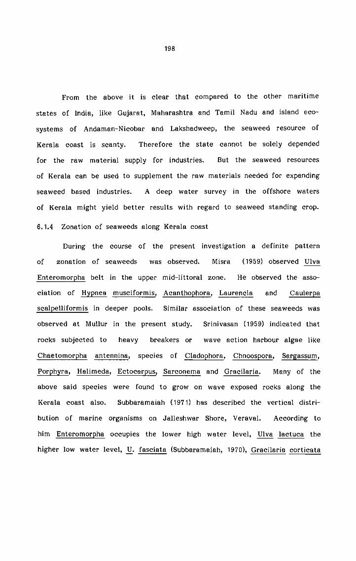
198

From the above it is clear that compared to the other maritime

states of India, like Gujarat, Maharashtra and Tamil Nadu and island eco

systems of Andaman-Nicobar and Lakshadweep, the seaweed resource of

Kerala coast is scanty. Therefore the state cannot be solely depended

for the raw material supply for industries. But the seaweed resources

of Kerala can be used to supplement the raw materials needed for expanding

seaweed based industries. A deep water survey in the offshore waters

of Kerala might yield better results with regard to seaweed standing crop.

6.1.4 Zonation of seaweeds along Kerala coast

During the course of the present investigation a definite pattern

of zonation of seaweeds was observed. Misra (1959) observed 1;

Enteromorpha belt in the upper mid-littoral zone. He observed the asso

ciation of Hypnea musciformis, Acanthophora, Laurencia and Caulerpa

scalpelliformis in deeper pools. Similar association of these seaweeds was

observed at Mullur in the present study. Srinivasan (1959) indicated that

rocks subjected to heavy breakers or wave action harbour algae like

Chaetomorpha antennina, species of Cladophora, Chnoospora, Sargassum,

Porphyra, Halimeda, Ectocarpus, Sarconema and Gracilaria. Many of the

above said species were found to grow on wave exposed rocks along the

Kerala coast also. Subbaramaiah (1971) has described the vertical distri

bution of marine organisms on Jalleshwar Shore, Veraval. According to

him Enteromorpha occupies the lower high water level, E lactuca the

higher low water level, 3. fasciata (Subbaramaiah, 1970), Gracilaria corticata

199.

and Hypnea musciformis extend to the lower low water level and Sargassum

tenerrimum extends to the sub-tidal region. Agadi and Untawale (1978)

observed along Goa coast that species of Chaetomorpha, Ulva and

Enteromorpha occur at higher levels, on rocks exposed to light where only

humidity is required for algal growth. Similar observation was made along

Kerala coast also. Kannan and Krishnamurthy (1978) observed that along

Coromandal coast Enteromorpha and Chaetomorpha inhabits all aquatic

biotypes suggesting the adaptability of these algae. Along the Kerala coast,

these two species of algae were recorded from all the five stations of

study, thus confirming the adaptability of these species. Agadi (1983)

observed along the Goa coast that the upper part of the algal zone,

Chlorophycean members like gig, Enteromorpha and Chaetomorpha were

present. This confirms the observation, made along the Kerala coast. The

author observed several rock pools in the mid algal zone at Goa, occupied

by Sargassum, Padina, Gracilaria corticata, Hypnea musciformis and

Grateloupia filicina. Several associations like Spatoglossum—Stoechofl)ermum

Dictyota and Gracilaria-Grateloupia-Ulva were observed along Goa coast.

As observed along Kerala, in Goa coast also the lower regions were occupied

by species of Sargassum, Gracilaria and Hypnea. Agadi (1985) observed

species like Porphyra, Ulva, Enteromorpha and Chaetomorpha along the

supra-littoral fringe of Karnataka coast as observed in the present study.

He observed the lower littoral zone to be occupied by species of Sargassum,

Dictyota, Laurencia, Acanthophora, Spyridea and Hypnea growing on rocky

substratum. Gracilaria corticata and Grateloupia lithophila grew in places

200

with strong wave action along Karnataka coast. These observations were

similar to those obtained in the present study. Jagtap (1985) observed

Caulerpa species growing in rock pools in Andaman islands. Chaetomorpha

and Ulva were growing at the high tide mark in the spray zone. Enteromorpha

intestinalis was observed to be growing in a sewage polluted area in Aberdeen

Jetty. These observations were similar to the one made in the present

study. Doty (1946) observed that critical tide factors are responsible for

vertical zonation of marine algae. Krishnamurthy (1965) observed that

nature of tides, extent of intertidal zone, physiographic factors and topo

graphy of the shore are the factors controlling the zonation of marine

algae on the Indian coasts. Dawson (1966) suggested that the adaptation

of different plants to varying conditions of light, temperature, exposure

to sea, salinity etc. results in distinct zonation of plants. Krishnamurthy

and Subbaramaiah (1970) observed the importance of shore types in the

zonation of Indian marine algae. Schwenke (1971) described wave action

and tidal currents as the important factors determining the local distribution

of seaweeds. Mathieson e_t Q (1977) described current regimes, topography

of shore and type of substrate as responsible for spatial variations in species

composition and abundance of benthic organisms. According to them vertical

substrates exposed to strong tidal currents are devoid of algae, while

recessed shoreline with sloping substrate exhibited good diversity and

abundance of intertidal organisms. Umamaheswara Rao and Sreeramulu

(1964) and Umamaheswara Rao (1978) observed that the differences in the

201

distribution of algae in relation to changes in tidal exposure and submergence

at Mandapam and Visakhapatnam coasts clearly indicate the importance

of tidal factor on the zonation of intertidal algae. Trono and Saraya (1987)

suggested that degree of water movement and availability of substrates

are major factors in controlling the horizontal distribution of large foliose

dominants. Mechanically strong macrophytes attained peak development

in the wave exposed portions of the reef, while mechanically weak species

were limited to protected portions.

6.2 BIOCHEMICAL COMPOSITION OF SEAWEEDS

Along the Kerala coast, brown algae recorded the highest protein

content followed by red -and green algae. The protein content in green

algae varied from 1% recorded in Valoniopsis pachynema to 20% recorded

in Caulerpa fastigiata. In brown algae it varied from 2.8% in Padina

gymnospora to 19.4% in E. tetrastromatica. In red algae, it varied from

2.3% in Grateloupia lithophila to 19.6% in Porphyra kanyakumariensis.

High carbohydrate content was recorded in both red and green algae.

Brown algae recorded the lowest carbohydrate content along Kerala coast.

In green algae, it varied from 2.75% recorded in Valoniopsis pachynema

to 75% in Caulerpa peltata. In brown algae it varied from 3.5% in Padina

gymnospora to 18.25% in Sargassum wightii. In red algae it varied from

6% in Hypnea valentiae to 55% in Grateloupia filicina.

202

Highest lipid content was recorded in brown algae followed by green

and red algae, along Kerala coast. Lipid content in green algae varied

from 0.5% in Valoniopsis pachynema to 18.75% in Cauleg>a sertularioides,

in brown algae it varied from 0.15% in Turbinaria conoides to 11.3% in

Dictyota dichotoma and in red algae it varied from 0.5% in Centrocerasclavulatum to 5.5% in Gracilaria foliifera.

Thus in the present study, it was observed that biochemical com

position varied markedly between different species of the same algal division,

suggesting that the quantity of biochemical constituents in an alga is

independent of its taxonomic division. Ogino (1955) studied variation in

protein nitrogen fraction in a number of Chlorophyceae, Rhodophyceae

and Ph?ophyceae. He found that these fractions varied with species. Lewis

(1967) observed that, although green algae were generally rich in protein,

Grateloupia lithophila belonging to red algae and Dictyota maxima belonging

to brown algae showed high protein contents. Andrea egg (1987) observed

that although relatively high protein content was recorded in red algae,

Eucheuma striatum belonging to red algae had low protein content. According

to them, brown seaweeds likewise did not yield uniformly low protein

contents. Dictyota sp. (brown alga) contained fair amount of protein.

Lewis and Gonzalves (1960) reported more than 28% protein in algae

from Bombay coast, while the maximum protein content recorded in algae

from Kerala coast was only 20% (Caulerpa fastigiata). Dhargalkar e_t il_

203

(1980) observed that protein content of marine algae from Maharashtra

varied from 10-33%, suggesting that protein content of seaweeds of Maha

rashtra was higher than that of Kerala. In Maharashtra, both protein

and carbohydrate contents were highest in red algae, but as was observed

in Kerala, green algae like Caulerpa and Ex/_a_ also recorded high carbohydrate

contents. Sitakara Rao and Tipnis (1964) estimated the crude protein content

of algae of Gujarat coast. Dave.and Parekh (1975) studied 8 genera of

green algae from Saurashtra. They observed significant variation in protein

contents in the same species of alga grown in different localities. In the

present study the protein content of M fasciata and the lipid content

of Gracilaria corticata varied significantly between stations. Porphyra

kanyakumariensis from Varkala recorded 15.13% protein, 21.75% carbohydrate

and 1.68% lipid. The same species from Mullur, recorded 18.47% protein,

22.37% carbohydrate and 2.86% lipid. Thus the biochemical constitution

were higher in the specimen collected from Mullur. Tewari it E (1968)

reported 16.01% protein content in Porphyra species from the east coast

of India. Protein content of 33.5% is reported in E. yezoensis from Japan.

Jagtap (1985) recorded 17.49% protein, 50.5% carbohydrate and 0.85% lipid

in Porphyra vietnamiensis. Durairatnam fig (1988) estimated the chemical

composition of some species of brown algae, along Rio Grande Do Norte,

Brazil. The protein content of Luis: gymnoswra varied from 6.6%-12.5%;

lipoid content from 0.94%—2.25% and carbohydrate content from 10.7%

41.2%. In the present study the protein content of Padina gymnospora

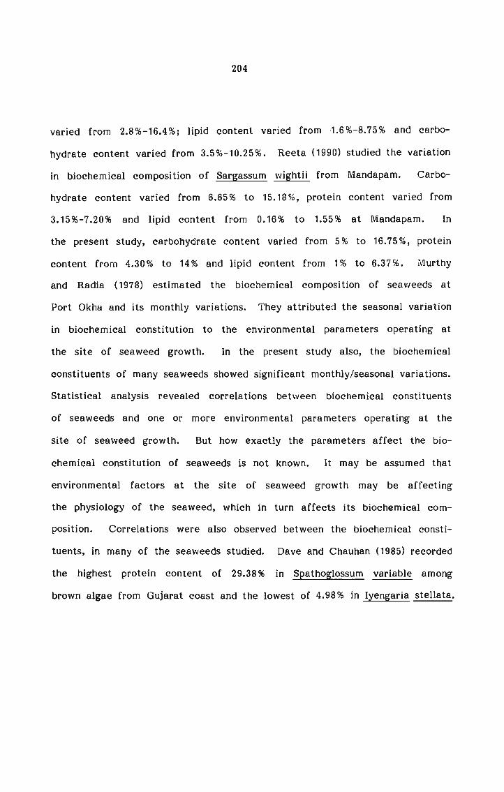
204

varied from 2.8%-16.4%; lipid content varied from 1.6%-8.75% and carbo

hydrate content varied from 3.5%-10.25%. Reeta (1990) studied the variation

in biochemical composition of Sargassum wightii from Mandapam. Carbo

hydrate content varied from 6.65% to 15.18%, protein content varied from

3.15%-7.20% and lipid content from 0.16% to 1.55% at Mandapam. In

the present study, carbohydrate content varied from 5% to 16.75%, protein

content from 4.30% to 14% and lipid content from 1% to 6.37%. Murthy

and Radia (1978) estimated the biochemical composition of seaweeds at

Port Okha and its monthly variations. They attributed the seasonal variation

in biochemical constitution to the environmental parameters operating at

the site of seaweed growth. In the present study also, the biochemical

constituents of many seaweeds showed significant monthly/seasonal variations.

Statistical analysis revealed correlations between biochemical constituents

of seaweeds and one or more environmental parameters operating at the

site of seaweed growth. But how exactly the parameters affect the bio

chemical constitution of seaweeds is not known. It may be assumed that

environmental factors at the site of seaweed growth may be affecting

the physiology of the seaweed, which in turn affects its biochemical com

position. Correlations were also observed between the biochemical consti

tuents, in many of the seaweeds studied. Dave and Chauhan (1985) recorded

the highest protein content of 29.38% in Spathoglossum variable among

brown algae from Gujarat coast and the lowest of 4.98% in Iyengaria stellata.

205

They also observed monthly and place-wise variation in biochemical compo

sition of seaweeds and attributed it to environmental factors operating

at the site of seaweed growth as in the present study. Average protein

content of brown algae recorded by them from Gujarat coast was higher

than that of Kerala. Dave e_t Q (1987) observed place-wise and monthly

variations in the protein contents of red seaweeds from Gujarat coast.

Dhargalkar (1979) observed seasonal variation in protein and carbohydrate

contents of seaweeds, but according to him lipid content did not show any

seasonal trends. But in the present study, lipid content of many of the

seaweeds studied, showed significant seasonal variations. Umamaheswara

Rao (1970) estimated the protein content of some seaweeds from Mandapam

coast. Most of the species recorded by him had a higher protein content

than the same species from Kerala, confirming the place-wise variation

in biochemical composition of seaweeds. Chennubhotla ga_l(1987) estimated

the biochemical composition of seaweeds from Mandapam. They observed

that green algae had the highest protein content while red algae the highest

carbohydrate and lipid contents. Compared to Mandapam, green algae

from Kerala recorded a lower protein content. But the maximum protein

content recorded in brown and red algae, was higher in Kerala, than

Mandapam. Maximum carbohydrate content recorded in green and red

algae was higher in Kerala than Mandapam. Lipid content of green and

brown algae from Kerala was higher than that of Mandapam. Reeta

gt_a_l (1990) recorded a higher protein content in green algae from Mandapam

206

compared to that of Kerala, but maximum values of carbohydrate and lipid

contents were higher in Kerala. They recorded 56.25% carbohydrate content

in green alga Caulerpa laeteverens from Mandapam. Along Kerala coast

also, species of Caulerpa recorded very high carbohydrate contents. Sumitra

e_tal (1980) studied seasonal variation in biochemical composition of seaweeds

of Goa coast, and suggested that biochemical composition did not show

marked seasonal changes, unlike the observation made in the present study.

Jagtap and Untawale (1980) estimated the protein and carbohydrate contents

of Caloglossa lepreiurii (red alga) from Zuari estuary, Goa. They observed

marked seasonal variation in biochemical composition of this alga, but have

suggested that environmental factors did not have any bearing on biochemical

composition of seaweeds. Jagtap and Untawale (1984) estimated the protein

contents of marine algae from Minicoy, Lakshadweep. It was found to

vary from 100-330 mg.g_1 dry weight. Kaliaperumal e_t Q (1987) estimated

protein contents of some seaweeds from Lakshadweep. According to them,

green algae recorded the highest protein content, red algae the highest

carbohydrate content and green algae the highest lipid content. But the

biochemical composition of most of the seaweeds from Lakshadweep reported

by them was lower compared to that of Kerala. Parekh e_t a_l (1983) and

Parekh 3 E (1985) estimated the biochemical composition of Enteromorpha.

Both protein and carbohydrate contents recorded by them were higher than

that in the present study. Mairh e_t a_l (1983) also studied the proximate

207

composition of Enteromorpha. The carbohydrate and lipid contents recorded

by the authors were higher than that recorded from Kerala. Solimabi

e_t_ al (1988) observed seasonal changes in protein and carbohydrate contents

in Hypnea musciformis and suggested that protein levels were highest when

nitrogenous nutrients were high. Temperature and salinity also according

to them had significant effect on biochemical composition of seaweeds.

Comparison of abundance and biochemical composition of seaweeds with

environmental factors by the authors indicated that during the period of

maximum growth, carbohydrates are comparatively higher than proteins.

In the present study also significant seasonal variation in biochemical com

position of seaweeds was observed. Sobha Q a_l (1988) observed that bio

chemical constitution varied with species of alga and place of its collection,

as observed in the present study. Black, (1954)., Harvey, (1955)., have

suggested that the chemical composition of algae does not depend only

on their specific characters but also on other factors like seasonal variation

in temperature, salinity, sea depth, stages of growth and part of plantstudied.

7.. SUMMARY

1. The main objective of the study was to collect information on the

ecology and basic biochemical composition of the seaweeds of Kerala coast.

2. For the convenience of study, the entire coast of Kerala was divided

into three zones, viz. 1) North zone 2) Central zone and 3) South zone.

Stations were fixed in each zone. Once every month, trips were undertaken

to each station for making ecological observations and for seaweed collection,

for a period of two years.

3. During the period of study, 52 species of seaweeds were collected

from Kerala coast, out of which 20 species belonged to Chlorophyta, 10

to Phieophyta and 22 to Rhodophyta. Thus Rhodophyceaen algae were most

abundant along Kerala coast, followed by Chlorophycean algae. Phféophycean

algae were relatively less along the Kerala coast.

4. Commercially important seaweeds of Kerala coast and the places

of their availability are given. This included 3 species of agarophytes,

7 species of agaroidophytes and 9 species of alginophytes. Names of

important edible seaweeds of Kerala are also given.

5. Zone-wise and station-wise distribution pattern of seaweeds of Kerala

coast are described. Number of seaweed species was maximum in North

zone (42 species), followed by South zone (37 species) and Central zone

(9 species). Out of the 42 species of seaweeds recorded from North zone,

13 were exclusive to North zone. Out of the 37 species of seaweeds

209

recorded from South zone, 8 were exclusive to South zone. Out of the

9 species of seaweeds recorded from Central zone, 1 was exclusive to

Central zone. No Phsiaophycean alga was present in the Central zone.

6. A definite zonation pattern was observed with regard to several

species of seaweeds in the present study. Horizontal zonation patternof seaweeds was observed at Saudi and Varkala.

7. Density of seaweeds was estimated to be 3971.25 gm/m2 at Mullur,

2047. 5 gm/m2 at Varkala, 1832.29 gm/m2 at Elathur, 1408.13 gm/m2 at

Thikkotti and 1387.5 gm/m2 at Saudi (wet weight). Density of each species

of seaweed, seasonal density of different divisions of algae and of some

selected species of seaweeds at each station are given.

8. Along Kerala coast, post monsoon recorded the highest seaweed

density followed by pre monsoon. Monsoon recorded the lowest seaweed

density. Green algal density was highest during monsoon, brown algal density

during pre monsoon and red algal density during post monsoon.

9. Frequency of occurrence of each species of seaweed along Kerala

coast is given.

10. Average standing crop of seaweeds along Kerala coast (based on

the stations studied) was estimated to be 2129.33 gm/m2. Out of this,

agarophytes constituted 13.5%, agaroidophytes 6.98% and alginophytes 9.06%.

Thus 29.53% of the seaweed standing crop of Kerala is constituted by

commercially important seaweeds.

210

11. Environmental data viz. atmospheric temperature, surface water

temperature, dissolved oxygen content, salinity, phosphate, nitrate and silicate

contents of ambient waters were recorded from Mullur, Varkala, Elathur,

Thikkotti and Saudi for a period of two years. Statistical significance

of seasonal variation in each environmental factor studied at Mullur, Varkala,

Elathur, Thikkotti and Saudi are given. Comparison of environmental data

recorded from different stations has been made. Statistical significance

of the variation between stations, with regard to each environmental factor

is also given. Correlation observed between environmental factors at each

station are described.

12. Effect of environmental factors on the density of some selected

seaweeds from each station was studied statistically and the results of

this study are presented. Density of each species of seaweed studied,

showed a correlation of some kind (positive or negative) with one or more

environmental factors studied. From this we can conclude that each species

of seaweed requires a specific combination of environmental factors for

its biomass production.

13. The protein, carbohydrate and lipid contents and the corresponding

calorific values of the seaweeds collected from Mullur, Varkala, Elathur,

Thikkotti and Saudi are given. Along Kerala coast, brown algae recorded

the highest protein content of 11.3%. Green and red algae recorded protein

contents of 10.2% and 10.3% respectively. Both green and red algae recorded

211

high carbohydrate contents of 22.6% and 22.5% respectively and brown

algae the lowest of 11.6%. Brown algae recorded the highest lipid content

of 5.6% followed by green algae with 4% and red algae the lowest with

1.9%.

14. Seasonal variation in biochemical composition of some selected sea

weeds from each station and their statistical significance are described.

15. Station-wise variation in protein, carbohydrate and lipid contents

of Ulva fasciata, E. lactuca, Chaetomorpha antennina and Gracilaria corticata

are given.

16. Parameters showing correlation (positive or negative) with protein,

carbohydrate and lipid contents of some seaweeds from each station were

identified statistically.

17. Thus in the present study, observations on the ecology of seaweed

flora of Kerala, their distribution and zonation pattern, monthly/seasonal

density of seaweeds at each station, frequency of occurrence, standing

crop, monthly/seasonal/place-wise data on physico—chemical characters of

ambient waters at the stations and their influence on seaweed density have

been made. This data will help us in the farming of economically important

seaweeds, by providing information on the ideal conditions of seaweed biomass

production. Biochemical observations on protein, carbohydrate and lipid

contents of different species of seaweeds will give us an idea of their

212

nutritive value. Seaweeds with high content of proteins, carbohydrates

and lipids can be recommended for food and feed formulations after subject

ing them to toxicological studies. The study on monthly/seasonal/place

wise variation in biochemical composition of seaweeds will provide necessary

information on the appropriate time and place of harvesting the algal species

for exploiting its constituents.

8. REFERENCES

Agadi, V.V.,1983. Intertidal ecology of marine algae along Anjuna coast,

Goa. Seaweed Res. Utiln. 6(1) : 27-30.

Agadi, V.V.,1985. Distribution of Marine Algae in the Littoral zone of

the Karnataka coast. In: Marine Plants (ed.) Krishnamurthy, V.

pp-35-42.

Agadi, V.V. and A.G. Untawale, 1978. Marine algal flora of Goa coast.

Seaweed Res. Utiln., 3 (1 dt 2) : 56-70.

Ananza-Corrales Rhodora, 1988. An Introduction to the seaweeds: their

characteristics and economic importance. Lecture presented during

ASEAN/UNDP/FAO Regional sma11—scale Coastal Fisheries Development

Project and Sea Farming Development and Demonstration Project

University of Philippines, Diliman, Quezon City.

Andrea H. Luistro, N.E. Montano, G.J.B. Cajipe and E.C. Laserna, 1987.

Protein content of some Philippine seaweeds with notes on the amino

acid content of Ulva lactuca Linn. and Gracilaria verrucosa (Huds.)

Papenfuss. The Philippine Journal of Science Monograph No.17,

pp,23—28.

Anon, 1981. Status report on Marine Algal resources of the Indian coast

for research and development, N.I.O., Goa. 12 p.

214

Anon, 1987. Seaweed Research and Utilisation in India. Bull. Cent. Mar.

Fish. Res. Inst. No.41.

Anon, 1988. Seaweed Resources of Kerala, Tamil Nadu and Lakshadweep.

C.M.F.R.I. news letter No.40 (April-June) on Seaweed Resources,

pp. 2-3.

Anon, 1989. Seaweed resources off the Tuticorin-Tiruchendur coast, Tamil

Nadu, India, Report of C.M.F.R.I. and C.S.M.C.R.I.

Anon, 1990. Present status of seaweed exploitation and seaweed industry

in India. Marine Fisheries Information Service of Cent. Mar. Fish.

Res. Inst. March 1990, pp. 7-8.

Arudpragasam, K.D. 1970. Zonation on two shores on the west coast of

Ceylon. J. mar. biol. Ass. India Vol.XII (1 6: 2) pp. 1-14.

Balakrishnan Nair, N., V. Sobha and M. Arunachalam, 1982. Algae from

Southern Kerala Coast. Indian J. mar. Sci., 11: 266-269.

Balakrishnan Nair, N., V. Sobha, R. Chandran, M. Rathiammal, P.K. Miranda,

S. Maya and H. Suryanarayanan, 1986. Algal Resources of Kerala

Coast 11 - An update list of Indian Marine Algae. Aquatic Biology,

Vol. VI, pp. 25-52.

Balakrishnan Nair, N., V. Sobha, R. Chandran, M. Rathiammal, S. Maya

and H. Suryanarayanan, 1990. Algal resources of Kerala coast X

- Occurrence and relative abundance of Phfeophyta along south

west coast of India. Presented at the Seminar on Phieophyceaein India, held at Madras.

215

Balakrishnan Nair, N., V. Sobha, R. Chandran, M. Rathiammal, S. Maya

and H. Suryanarayanan, 1990. Algal resources of Kerala coast IX

- Occurrence and relative abundance of Chlorophyceae along south

west coast of India. Seaweed Res. Utiln. 12 (1 & 2) : 125-135.

Balasundaram, A., 1985. Seasonal succession of algae in the mid-algal

zone on the Thiruchendur shore. In: Marine Plants (ed.) Krishna

murthy, V. pp. 179-190.

Barnes, H. and J. Blackstock, 1973. Detailed investigation of the sulpho

vanillin method for total lipid. J. exp. mar. Biol. Ecol, 12 : 103

118.

Bersamin, S.V., 1974. Some seaweeds consumed fresh in Philippines. The

Philippines. Jour. of Fish. 8(2) : 183-189.

Bhanderi, P.P. and Y.B. Raval, 1975. Possibility of seaweed cultivation

along the Gujarat coast. Seafood Export Jour., 7(12) : 33-36.

Bhanderi, P.P. and Y.A. Trivedi, 1975. Seaweed resources of Hanumandandi

reef and Vumani reef near Okha Port. Indian J. mar. Sci., 4 (1): 97-99.

Bird, K.T. and P.H. Benson, 1987. Seaweed Cultivation for renewable

resources. Developments in Aquaculture and Fisheries Science,Vol. 16.

Bird, C.J. and J. McLachlan, 1986. The effect of salinity on the distribution

of species of Gracilaria Grev. (Rhodophyta, Gigartinales) : An experi

mental assessment. Bot. Mar. Vol.XXlX, pp. 231-238.

216

Black, W.A.P. 1954. Constituents of marine algae. Ann. Rep. Chem. Soc.,

50 : 322-335.

Blinks, L.R., 1951. Physiology and biochemistry of algae. In: Manual of

phycology (Ed. Smith, G.M.) pp. 263-291.

Block, R.J. and K.W. Weiss, 1956. Amino acid handbook. Methods and

results of protein analysis Spring field, Illinois, U.S.A.

Bonotto, S., 1976. Cultivation of plants. Multicellular plants. In: Kinne,O.

(ed.). Marine Ecology Vol.3. cultivation Part I. Wiley, New York.

Bryan, P.G., 1975. Food habits, functional digestive morphology and assimi

lation efficiency of the rabbit-fish, Siganus spinus (Pisces, Siganidae)

in Guam. Pac. Sci., 29 (3) : 269-277.

Chacko, P.I. and C. Malupillai, 1958. Studies on utilisation of seaweed

resources of Madras state. Contr. Mar. Biol. St. Krusadai Island,

6: 1-12.

Chapman, V.J., 1943. Zonation of marine algae on the sea shore. Proc.

Linn. Soc. Lond. 154, 239-253.

Chapman, V.J., 1955. Marine algal ecology. Bot. Rev. 23, 320-350.

Chapman, V.J., 1970. Seaweeds and their uses. 2nd ed. Methusen, London.

Chapman, V.J., 1978. Coastal vegetation. 2nd ed. Pergamon Press Ltd.

Chapman, V.J. and D.J. Chapman, 1975. The algae, Macmillan Press Ltd.,

London and Basingstoke, 2nd ed. pp. 497.

217

Chapman, V.J. and D.J. Chapman, 1980. Seaweeds and their uses. 3rd

ed. Chapman and Hall, London. pp. 62-97.

Chaturvedi, D.K., S.S. Verma and S.P. Khare, 1979. Studies on Feeding

Marine Algae (Gracilaria meal) in Laying White Leghorn birds. Int.

Symp. on Marine Algae of the Indian Ocean region, (Abstract)

p.51

Chauhan, V.D., 1978. Report on the survey of marine algal resources of

Maharashtra coast. Salt. Res. Ind., 14 (1) : 1-10.

Chauhan, V.D. and V. Krishnamurthy, 1968. An estimate of algin bearing

seaweeds in the Gulf of Kutch. Curr. Sci. 37: p. 648.

Chauhan, V.D. and O.P. Mairh, 1978. Report on the survey of marine

algal resources of Saurashtra coast, India. Salt. Res. Ind., 14 (2): 21-41.

Chennubhotla, V.S.K., 1977. Food from the sea. Food from the seaweeds.

Seaweed Export Journal, Vol. IX, No.3, pp. 1-4.

Chennubhotla, V.S.I(., N. Kaliaperumal and S. Kalimuthu, 1981. Seaweed

recipes and other practical uses of seaweeds. Seafood export Journal

Vol. XIII, No.10, pp. 1-4.

Chennubhotla, V.S.K. and N. Kaliaperumal, Seaweed resources of Kerala

coast. (unpublished project report of Cent. Mar. Fish. Res. Inst.

1983).

Chennubhotla, V.S.K., B.S. Ramachandrudu, P. Kaladharan and S.K. Dhar

maraja, 1986. Seaweed resources of Kerala coast. Presented at

the seminar on Fisheries Research and Development in Kerala,Trivandrum.

218

Chennubhotla, V.S.K., M. Najmuddin, J.R. Ramalingam and N. Kaliaperumal,

1987. Biochemical composition of some marine algae from Mandapam

coast (South India). (unpublished project report of Cent. Mar. Fish.

Res. Inst. 1987).

Chennubhotla, V.S.K., N. Kaliaperumal and S. Kalimuthu, 1987. Common

seaweed products. Bull. Cent. Mar. Fish. Res. Inst. No.41. pp.26-30.

Chennubhotla, V.S.K. and Susan Mathew, 1989. Economic green algae and

their possible utilization in India. Presented at the National Workshop

on Taxonomy of Economically Important Marine Algae of India held

at the Mandapam Regional Centre of C.M.F.R.I. in March, 1989.

Chennubhotla, V.S.K., Susan Mathew and Imelda Joseph, 1990. A note

on the occurrence of Porphyra kanyakumariensis (Bangiales,Rhodophyta)

along the Kerala coast. Seaweed Res. Utiln., 13 (1) : 1-4.

Chennubhotla, V.S.K., N. Kaliaperumal and M.S. Rajagopalan, 1990. Seaweed

culture in India - An appraisal. Bull. Cent. Mar. Fish. Res. Inst.

No.44. pp. 394-402.

Conover, J.T., 1964. The ecology, seasonal periodicity and distribution

of benthic plants in some Texas lagoons. Bot. Mar. 7 : 4-41.

Conover, J.T., 1968. The importance of natural diffussion gradients and

transport of substances related to benthic marine plant metabolism.

Bot. Mar. 11: 1-9.

219

Coutinho, R. and U. Seelinger, 1984. The horizontal distribution of the

benthic algal flora in the Patos Lagoon estuary, Brazil, in relation

to salinity, substratum and wave exposure. J. Exp. Mar. Biol. Ecol.

80: 247-257.

Daly, M.A. and A.C. Mathieson, 1977. The effects of sand movement on

Intertidal seaweeds and selected Invertebrates at Bound Rock, New

Hampshire, U.S.A. Marine Biology, 43, 45-55.

Dave, M.J. and R.G. Parekh, 1975. Protein content of green seaweeds

from Saurashtra coast. Salt. Res. Ind., 11 (2) : 41-44.

Dave, M.J., S.K., Garg and E.R.R. Iyengar, 1977. Assessment of the possibi

lity of seaweeds to be utilised as supplementary animal feed. Salt.

Res. Ind., 13 (1 6c 2) : 33-40.

Dave, M.J., R.G. Parekh, S.K. Garg and D.J. Metha, 1979. Preparation

of seaweed meal for feeding of farm animals. Salt Res. Ind., 15(2) : 34-38.

Dave, M.J. and V.D. Chauhan, 1985. Protein content of brown seaweeds

from Gujarat coast, West coast of India. Indian Jour. Mar. Sci.,

Vol. 14, pp. 46-47.

Dave, M.J., R.G. Parekh, B.K. Ramavat, Y.A. Doshi and V.D. Chauhan,

1987. Protein contents of red seaweeds from Gujarat coast. Seaweed

Res. Utiln. 10 (1) : 17-20.

Dawson, E.Y., 1966. Marine Botany : An Introduction. Holt, Rinehart

and Winston Inc, New York. 37 pp.

220

Dawes, C.J., F.M. Scott and E. Bomler, 1981. Marine Botany John Wiley

and Sons, New York, Brisbane, Toronoto, Singapore.

Desai, B.N., 1967. Seaweed resources and extraction of alginate and agar.

Proc. Semi. Sea. Salt. and Plants, C.S.M.C.R.I. Bhavnagar. pp. 343

351.

Dhargalkar, V.K., 1979. Biochemical studies on Ulva reticulata Forsskal.

Proc. Int. Symp. Marine Algae of the Indian ocean region, C.S.M.C.R.I.,

Bhavnagar, p. 40 (Abstract).

Dhargalkar, V.K., T.G. Jagtap and A.G. Untawale, 1980. Biochemical consti

tuents of seaweeds along the Maharashtra coast. Indian J. Mar.

Sci., 2 (4) : 297-299.

Dhargalkar, V.K., V.V. Agadi and A.G. Untawale, 1981. Occurrence of

Porphyra vietnamiensis (Bangiales, Rhodophyta) along the Goa coast.

Mahasagar-Bulletin of N.I.O. 14(1) : 75-77.

Doty, M.S. and J. Newhouse, 1954. The distribution of marine algae into

estuarine waters. Amer. J. Bot. 41 : 508-515.

Doty, M.S., 1946. Critical tide factors that are correlated with the vertical

distribution of marine algae and other organisms along the Pacific

coast. Ecology, 27, 315-328.

Doty, M.S., 1971 a. Antecedent event influence on benthic marine algal

standing crops in Hawaii. Exp. mar. Biol. Ecol., Vol.6, pp. 161166.

221

Doty, M.S., 1971 b. Measurement of water movement on benthic marine

algal growth. Bot. Mar. 14 : 32-35.

Dubois, M., K.A. Gilles, J.K. Hamilton, P.A. Roberts and F. Smith, 1956.

Colorimetric method for determination of sugars and related sub

stances. Anal. Chem. 28: 350-356.

Durairatnam, M. and V. Raghunathamuthaliar, 1973. Ecological study of

marine algae on the littoral and sublittoral zone off Mandativu.

J. mar. biol. Ass. India, 15(2) : 652-657.

Durairatnam, M., Luci F. da Silva, Guacryra G.M. de Farias and Edda L.

Leite, 1988. Chemical composition of some species of marine brown

algae collected in the sublittoral areas of the state of Rio Grande

do Norte. Seaweed Res. Utiln. 11(1) : 45-49.

Fujiwara-Arasaki, T., M. Mino and M. Kuroda, 1983. The protein value

in human nutrition of edible marine algae in Japan. Proc. XI Int.

Seaweed. Symp. China, 1983, 74 p. (Abstract).

Garber, P., J.D. Dutcher, E.G. Adams and J.R. Sherman, 1958. Protective

effects of seaweed extracts for chicken embryos infected with

influenza B or mumps virus. Proc. Soc. Exp. Biol. Med. 99, 590593.

Gaur, K., T. Ramakrishna, D.P. Subbaraju and M.S. Murthy, 1982. Ecological

studies on Ulva lactuca L. from Veraval, India. Hydrobiologia, 89,89-94.

222

Gavino, C. Trono, Jr. and Teresita A. Buchan-Antalan, 1987. Biomass pro

duction in Acanthophora associated algal communities in Bacoor

Bay, Cavite, Philippines. The Philippine Journal of Science, Monograph

No.17, pp. 1-10.

Gavino C. Trono, Jr. and Anant Saraya, 1987. The structure and distribution

of macrobenthic algal communities on the reef of Santiago Island,

Bolinao, Pangasinan. The Philippine Journal of Science, Monograph

No.17, pp. 63-81.

Gavino C. Trono, Jr., 1988. "Seaweed Ecology" Influence of environmental

factors on the structure, phenology and distribution of seaweeds

communities. Lecture by Gavino Trono, Jr. during ASEAN/UNDP/FAO

Regional small-scale Coastal Fisheries Development Project and

Sea Farming Development and Demonstration Project University

of Philippines, Diliman, Quezon City.

Gopalakrishnan, P., 1970. Some observations on the shore ecology of

the Okha coast. J. mar. biol. Ass. India, 12 (1 6: 2) : 15-34.

Gopinathan, C.P. and R. Panigraphy, 1983. Seaweed Resources. Bull.

Cent. Mar. Fish. Res. Inst. No.34. on Mariculture potential of Andaman

and Nicobar Islands. An indicative Survey, pp. 47-51.

Gopinathan, C.P. and P. Parameswaran Pillai, 1974. Protein from the sea.

Seafood Export Journal, Vol. VI, No.5, 1-7.

Harvey, H.W., 1955. The chemistry and fertility of the seawater, London,

Cambridge University Press.

Hoppe, H.A., 1966. Nahrungasmittel aus Meeresalgen. Bot. mar. 9 (Suppl.)

: 18-40.

223

Inger Wa11entinus., 1983. Partitioning of productivity and nutrient uptake

between annual and perennial seaweeds in a Baltic Archipelago area.

Proc. XI Int. Seaweed Symp., China (Abstract).

Iverson, E.S., 1976. Farming the edge of the sea. Fisheries News Books

Ltd., Surrey, England.

Jagannathan, V. and R. Venkatakrishnan, 1979. Nutritional investigations

of seaweeds in chick ration. Proc. Int. Symp. on Marine Algae

of the Indian Ocean Region, C.S.M.C.R.I., Bhavnagar, India, pp.

49-51 (Abstract).

Jagtap, T.G., 1985. Studies on Littoral Flora of Andaman Islands. In:

Marine Plants (ed.) Krishnamurthy, V. pp. 43-50.

Jagtap, T.G., 1985. Major metabolites from Monostroma sp. Thuret. and

Porphyra vietnamensis Tan. et. I-lo. In: Marine Plants (ed.) Krishna

murthy, V., pp. 89-92.

Jagtap. T.G., 1986. Studies on the associated flora of the mangrove environ

ment. Proc. Natl. Symp. Biol. Utiln. Conr. Mangroves, Kolhapur,

pp. 180-187.

Jagtap, T.G. and A.G. Untawale, 1980. Some ecological and biochemical

observations on Caloglossa lepreiurii (Harvey) from Zuari estuary,

Goa. Seaweed Res. Utiln. 4(1): 17-24.

Jagtap, T.G. and A.G. Untawale, 1984. Chemical composition of marine

macrophytes and their surrounding water and sediments, from Minicoy,

Lakshadweep. Indian Jour. Mar. Sci. Vol. 13, pp. 123-125.

224

Jones, W.E., 1959. Experiments on some effects of certain environmental

factors on Gracilaria verrucosa (Hudson). Papenfuss. J. Mar. Biol.

Assoc., U.K. 38: 153-167.

Kaliaperumal, N. and G. Pandian, 1984. Marine algal flora from some

localities of South Tamil Nadu coast. J. Mar. biol. Ass. India.,

Vol. 26 (1 6L 2) pp. 159-164.

Kaliaperumal, N., V.S.K. Chennubhotla, S. Kalimuthu, J.R. Ramalingam,

M. Selvaraj and M. Najmuddin, 1987. Chemical composition of

seaweeds. Bull. Cent. Mar. Fish. Res. Inst. No.41. on Seaweed

Research and Utilisation in India, pp. 31-51.

Kaliaperumal, N., V.S.K. Chennubhotla, N. Najmuddin, J.R. Ramalingam

and S. Kalimuthu, 1987. Biochemical composition of some common

seaweeds from Lakshadweep. (unpublished project report of Cent.

Mar. Fish. Res. Inst. 1987).

Kaliaperumal, N., P. Kaladharan and S. Kalimuthu, 1989. Seaweed and

seagrass resources. Bull. Cent. Mar. Fish. Res. Inst. No.43. on Marine

Living Resources of the Union Territory of Lakshadweep, pp. 162

175.

Kannan, L. and K. Krishnamurthy, 1978. A survey of the algae of the Porto

Novo region (Coramande1 coast, Bay of Bengal). Seaweed Res. Utiln.

3: 1-4.

Koshy, T.K. and C.C. John, 1948. Survey of Gracilaria resources of Travan

core coast. Dept. Res. Univ. Travancore, Rep. for September, pp.53-55.

225

Krishnamurthy, V., 1965. Some general considerations on zonation of marine

algae on the Indian coasts. Proc. Sem. Sea, Salt and Plants,C.S.M.C.R.I., Bhavnagar, (ed.) Krishnamurthy, V. pp. 219-223.

Krishnamurthy, V., 1971. Seaweed Resources of India and their utilisation.

Seaweed Res. Utiln. Vol. 1, pp. 55-66.

Krishnamurthy, V., 1985. Towards a marine algal flora of India. In: Marine

Plants, their Biology, Chemistry and utilisation. Proc. All India.

Symp. mar. plants, Goa, 1985. pp. 1-16.

Krishnamurthy, V., 1990. Algae as Food. Lecture presented at the workshop

on algal products and seminar on Phaéophyceae in Indiaaheld by seaweed

research and utilisation association at Madras.

Krishnamurthy, V., R. Venugopal, James G. Thiagaraj and H.N. Shah, 1967.

Estimating drift seaweeds on the Indian coasts. Proc. Sem. Sea,

Salt and Plants, C.S.M.C.R.I., Bhavnagar, pp. 315-320.

Krishnamurthy, V. and K. Subbaramaih, 1970. The importance of shore

types in intertidal ecology of Indian marine algae. Pro. Indian Nat.

Sci. Acad. Vol. 38 B, Nos. (3 <5: 4), 259-266.

Krishnamurthy, K., S. Sambasivan, P. Subramanian and R. Rajan, 1982.

Seaweeds: Their use as a source of feed in the culture of prawns.

Seaweed Res. Utiln. 5(2) : 61-67.

Krishnamurthy, V. and M. Baluswami, 1984. The species of Porphyra from

the Indian region. Seaweed Res. Utiln. 4(1) : 31-38.

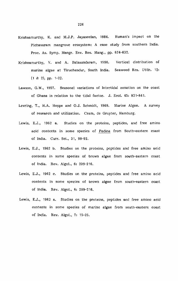
226

Krishnamurthy, K. and M.J.P. Jayaseelan, 1984. Human's impact on the

Pichavaram mangrove ecosystem: A case study from southern India.

Proc. As. Symp. Mangr. Env. Res. Mang., pp. 624-632.

Krishnamurthy, V. and A. Balasundaram, 1990. Vertical distribution of

marine algae at Tiruchendur, South India. Seaweed Res. Utiln. 12:

(1 6c 2), pp. 1-22.

Lawson, G.W., 1957. Seasonal variations of Intertidal zonation on the coast

of Ghana in relation to the tidal factor. J. Ecol. 45: 831-841.

Levring, T., H.A. Hoppe and O.J. Schmidt, 1969. Marine Algae. A survey

of research and utilization. Cram, de Gruyter, Hamburg.

Lewis, E.J., 1962 a. Studies on the proteins, peptides, and free amino

acid contents in some species of Padina from South-eastern coast

of India. Curr. Sci., 31, 90-92.

Lewis, E.J., 1962 b. Studies on the proteins, peptides and free amino acid

contents in some species of brown algae from south-eastern coast

of India. Rev. Algol., 6: 209-216.

Lewis, E.J., 1962 c. Studies on the proteins, peptides and free amino acid

contents in some species of brown algae from south-eastern coast


Lewis, E.J., 1963 a. Studies on the proteins, peptides and free amino acid

contents in some species of marine algae from south-eastern coast


Lewis,

Lewis,

Lewis,

Lewis,

Lewis,

Lewis,

Lewis,

Lewis,

227

E.J., 1963 b. The proteins, peptides and free amino acid composition

in species of Acanthophora from south east coast of India. Rev.

Algol., 7: 237-241.

E.J., 1963 c. Studies on the proteins, peptides and free amino acid

contents in some species of red algae from south-eastern coast

of India. Proc. natn. Inst. Sci. India, 29: 137-145.

E.J., 1963 d. Studies on fortnightly analysis of proteins, peptides,

and free amino acids in some marine algae from Bombay. Proc.

natn. Inst. Sci. India, 29: 363-386.

J.R., 1964. The ecology of rocky shores, XII, 323 pp. London: English

Universities Press Ltd.

E.J., 1967. A review of protein, peptide and free amino acid contents

of Indian Marine Algae. Proc.Semi. Sea, Salt and Plants, C.S.M.C.R.I.,

Bhavnagar, pp. 296-308.

E.J. and E.A. Gonzalves, 1959 a. Studies on the free amino acid

contents of some marine algae from Bombay. Jour. Univ. Bombay,

28: 1-5.

E.J. and E.A. Gonzalves, 1959 b. Amino acid contents of the erect

and creeping fronds of species of Caulerpa from Bombay. Jour.mar. biol. Ass. India, 1: 54-56.

E.J. and E.A. Gonzalves, 1959 c. Studies on the free amino acid

contents of species of Caulerpa from Bombay. Jour. mar. biol.

Ass. India, 1: 203-205.

228

Lewis, E.J. and E.A. Gonzalves, 1960. Amino acid contents of some marine

algae from Bombay. New Phytol, 59: 109-115.

Lewis, E.J. and E.A. Gonzalves, 1962 a. Studies on the protein, peptide

and free amino acids in cystocarpic and tetrasporic plants of

Agardhiella robusta from Bombay. New Phytol. 61: 288-290.

Lewis, E.J. and E.A. Gonzalves, 1962 b. The protein, peptide and amino

acid contents of some species of marine algae from Bombay. Ann.

Bot. N.S., 26: 301-316.

Lewis, E.J. and E.A. Gonzalves, 1962 c. Periodic studies of the proteins,

peptides and free amino acid in Enteromorpha prolifera, f. capillaris

and Ulva lactuca var. rigida. Ann. Bot. N.S., 26: 317-327.

Lowry, O.l1'., N.J. _Rosebrough, A.L. Farr and R.J. Randall, 1951. Protein

measurement with Folin-phenol reagent. J. Biol. Chem. 193: 265

275.

Mairh, O.P., R.G. Parekh, V.D. Chauhan, P.S. Rao and D.J. Mehta, 1983.

Ecology, culture and chemical constituents of Enteromorpha from

Gujarat coast. Seaweed Res. Utiln. 6(1): 1-22.

Masao Ohno, 1983. Observation on the floating seaweeds in near shore

water of Southern Pacific of Japan. Proc. XI Int. Seaweed Symp.

China p. 193 (Abstract).

Mathieson, A.C., Eleanor Tveter, Maureen Daly and J. Howard, 1977. Marine

Algal Ecology in a New Hampshire Tidal Rapid. Bot. mar. Vo1.XX,

pp. 277-290.

229

McHugn, D.G. and B.V. Lanier, 1984. Korea's edible seaweed trade. Infofish

Marketing Digest. No.3/84, pp. 17-19.

Mehta, V.C., B.S. Trivedi, K.K. Bokil and I‘-/I.R. Narayana, 1967. Seaweeds

as manure: 1—Studies on nitrification. Proc. of the Seminar on Sea,

Salt and Plants, C.S.M.C.R.I., Bhavnagar, pp. 357-365.

Misra, J.N., 1959. The ecology, distribution and seasonal succession of

the littoral algae on the west coast of India. Proc. of the Symp.

on Algology, pp. 187-203.

Misra, J.N., 1965. The Phfaophyceae of the west coast of India. Proc.

of the Seminar on Sea, Salt and Plants, Bhavnagar, pp. 227-233.

Munda, 1., 1978. Salinity dependent distribution of benthic algae in estuarine

areas of Icelandic fjords. Bot. Mar. 21: 451-468.

Murthy, M.S., M. Battacharya and R. Radia, 1978. Ecological studies on

the Intertidal Algae at Okha (India). Bot. mar. Vol.XXl, pp. 381

386.

Murthy, M.S. and P. Radia, 1978. Eco-biochemical studies on some econo

mically important intertidal algae from Port Okha (India). Bot.

Mar., 21(7): 417-422.

Murthy, C.S. and V.V.R. Varadachari, 1980. Topographic changes of the

beach at Valiathura, Kerala. Indian J. mar. Sci., Vol.9, pp. 3134.

Naqvi, S.W.A., B.D. Solimabi, S.Y. Kamat, L. Fernandes and C.V.G. Reddy,

1981. Screening of some marine plants from the Indian coast for

biological activity. Bot. Mar., 24 (1): 51-55.

230

Nienhius, P.H., 1971. The use of permanent sample plots in studying the

quantative ecology of algae in salt marshes. Proc. VII Int. Seaweed

Symp. Sappro, Japan, 251-254.

Ogino, C., 1955. Biochemical studies on the nitrogen compounds of algae.

Jour. Tokyo Univ. Fish., 41, 107-152.

Paciente A. Cordero, 1983. Some sea vegetables from Luzon island,

Philippines. Proc. XI Int. Seaweed Symp. China, 1983, pp.50 (Abstract).

Parekh, K.S., H.H. Parekh, H.M. Mody and P.S. Rao, 1983. Total lipid,

sterol and chlorophyll contents of some Indian seaweeds. Seaweed

Res. Utiln. 6(1) : 23-25.

Parekh, R.G., Y.A. Doshi, K.H. Mody, B.K. Ramavat and V.D. Chauhan,

1985. Biochemical investigations of Enteromoflha flexuosa (Wu1f.)

J. Ag. of Gujarat Coast. Seaweed Res. Utiln. 8 (1 dc 2) : 5-11.

Prasanna Varma, R., 1959. Studies on the succession of marine algae on

a fresh substratum in Palk Bay. Proc. of Indian Acad. of Sci. Vol.

XLIX, 1959, 245-262.

Prescott, G.W., 1969. The Algae: A Review, Thomas Nelson and Sons Ltd.,

London.

Rama Rao, K., 1972. Role of critical tide factor in the vertical distri

bution of Hypnea musciformis (Wu1f.) Lamour. Proc. Indian. Natl.

Sci. Aca. Vol. 38 B (3 as: 4) : 267-272.

231

Reeta Jayasankar, 1990. Seasonal variation in biochemical constituents

of Sargassum wightii (Greville) with reference to alginic acid content.

(Submitted for publication).

Reeta Jayasankar, J.R. Ramalingam and N. Kaliaperumal, 1990. Biochemical

composition of some green algae from Mandapam coast. Seaweed.

Res. Utiln. Vol. 12 (1 6c 2), 37-40.

Richardson, W.D., 1969. Some observations on the ecology of Trinidad

marine algae. Proc. VI Int. Seaweed Symp. Spain, 357-363.

Rodhe, W., 1948. Environmental requirements of fresh water plankton

algae. Symbolae Botan. 10: 1-49.

Sampathkumar, P., M. Ganesan, R. Karina, C. Govindasamy, K. Rajendran

and L. Kannan, 1990. Seasonal variation in distribution and biomass

of Phieophycean algae in the Gulf of Mannar. Presented at the

Seminar on Phaeophyceae in India held at Madras, 1990.

Schwenke, H., 1971. Water movement, 2. Plants. In: Marine ecology, Vol.1,

Pt. 2, edited by O. Kinne, Wiley — Inter—science, London, 1091

1121.

Shakuntala Moorjani, 1979. Seasonal changes in the marine algal flora

on the Kenya coast. Proc. Int. Symp. Marine Algae of the Indian

ocean region, C.S.M.C.R.I., Bhavnagar, (abstract) p. 8.

Shunula, J.P., 1983. Biomass trends in Ulva fasciata Delile and Ulva pulchra

Jaasund (Chlorophyta, Ulotrichales) in Dar-es-Salaam-Tanzania. Seaweed

Res. Utiln. 6(2) : 49-52.

232

Shunula, J.P., 1985. A preliminary check list of Ph'/aeophyta and Rhodophyta

of economic importance on five shores of Zanzibar. Seaweed Res.

Utiln. 7: (2), 65-70.

Silas, E.G., 1987. Prospects of seaweed research and utilisation. Bull.Cent. Mar. Fish. Res. Inst. No.41. on Seaweed Research and utili

sation in India, 1987, pp. 80-81.

Silas, E.G., V.S.K. Chennubhotla and N. Kaliaperumal, 1983. Seaweed pro

duction, their products and utilisation in India. Proc. XI Int. Seaweed.

Symp. China, 1983, 225 p. (Abstract).

Sitakara Rao, V. and U.K. Tipnis, 1964. Protein content of marine algae

from Gujarat coast. Curr. Sci., 33: 16-17.

Sivalingam, P.M., 1983. Biotechnological economic utilization of marine

algae in Malaysia for rural communities. Proc. XI Int. Seaweed.

Symp. China, 1983. 226 p. (Abstract).

Sobha, V. and N. Balakrishnan Nair, 1983. Marine Algae of Kerala 11;

Report on a collection from Varkala, Kovalam, Poovar and Cape

Comorin. Mahasagar — Bulletin of N.I.O. 16(4): 469-471.

Sobha, V. and N. Balakrishnan Nair, 1985. Marine Algae of the South

west coast of India. In: Marine Plants (ed.). Krishnamurthy, V.

pp. 17-24.

Sobha, V., K.S. Maya Devi and T. Vasudevan Nair, 1988. Proximate com

position of certain algae at Kovalam, S.W. coast of India. Seaweed

Res. Utiln. 11(1): 31-38.

233

Solimabi, B.D., S.Y. Kamat, L. Fernandes and C.V.G. Reddy, 1980. Seasonal

changes in Carrageenan and other biochemical constituents of Hypnea

musciformis. Indian J. Mar. Sci. Vol. 9, 134-136.

Sreenivasa Rao, P., E.R.R. Iyengar and F. Thivy, 1964. Survey of algin

bearing seaweeds at Adatra reef, Okha. Curr. Sci. 33: 464-465.

Sreenivasa Rao, P., K.S. Parekh, H.H. Parekh, S.B. Trivedi and B.A. Dave,

1979. Effect of seaweed extracts on Micobacterium tuberculosis

Proc.‘ Int. Symp. Marine Algae of the Indian Ocean Region,

C.S.M.C.R.I., Bhavnagar, India, p. 47 (Abstract).

Srinivasan, K.S., 1959. Distribution patterns of marine algae in Indian

seas. Proc. Symp. on Algology, pp. 219-242.

Srinivasan, K.S., 1969. Phycologia indica, Vol. 1.

Stephenson, T.A., 1943. The causes of vertical and horizontal distribution

of organisms between tide marks in South Africa. Proc. Linn. Soc.

Lond. 154, 219-234.

Stephenson, W.A., 1974. Seaweed in Agriculture and horticulture, 3rd ed.,

Rateaver, Pauma Valley, Cal., 241 pp.

Strickland, J.D.H. and T.R. Parsons, 1968. A practical hand book of seawater

analysis. Bull. Fish. Res. Bd. Canada, 167: 1-311.

Subbaramaiah, K., 1970. Growth and Reproduction of Ulva fasciata Delile.

in Nature and in culture. Bot. Mar., 8: 25-27.

234

Subbaramaiah, K., 1971. Distribution of marine organisms on the Jalleshwar

Shore, Veraval. Seaweed Res. Utiln. Vol.1, pp. 19-29.

Subbaramaiah, K., M.R.P. Nair and V. Krishnamurthy, 1977. Distribution

pattern of Marine algae on the shore of Pamban. Seaweed Res.

Util., Vol. 2(2): 74-77.

Subbaramaiah, K., K. Rama Rao, M.R.P. Nair, V.S.K. Chennubhotla and

M. Paramasivam, 1979 a. Marine Algal Resources of Tamil Nadu.

Proc. Int. Symp. Marine Algae of the Indian Ocean Region,

C.S.M.C.R.I., Bhavnagar, India, p. 14 (Abstract).

Subbaramaiah, K., K. Rama Rao and M.R.P. Nair, 1979 b. Marine Algal

Resources of Lakshadweep. Proc. Int. Symp. Marine Algae of the

Indian Ocean Region. C.S.M.C.R.I., Bhavnagar, India, pp. 6-7 (Abstract).

Subbaramaiah, K., 1987. Resources, Management and possible cultivation

of some economic seaweeds in India. Proc.Internl. Symp. on phycology.

Univ. Madras, 8-13 January, 1987.

Subba Rao, P.V., K. Rama Rao, M.R.P. Nair and K. Subbaramaiah, 1985.

A systematic list of marine algae from Andhra Pradesh and their

distribution. In: Marine plants (ed.) Krishnamurthy, V. pp. 2934.

Subramanyan, R., 1967. Methods of assessing seaweed resources and pro

blems. Proc. Semi. Sea, Salt and Plants, C.S.M.C.R.I., Bhavnagar,

pp. 311-314.

235

Subramanyan, R. and C.P. Gopinathan, 1971. Vegetable resources from

the sea. Seaweed export Journal, Vol.III, No.1, pp. 1-7.

Sumitra Vijayaraghavan, M.D. Rajagopalan and M.V.M. Wafar, 1980. Seasonal

variations in biochemical composition of some seaweeds from Goa

coast. Indian J. Mar. Sci., Vol. 9, pp. 61-63.

Swamy, P.K., 1990. Export prospects for Indian seaweeds. Presented in

the Group Discussion on seaweed resources, farming and utilisation

organised by C.M.F.R.I. at Mandapam Camp.

Tamiya, H., 1960. Role of Algae as food. Proc. of the Symp. on Algology

pp. 379-389.

Tewari, A., M. Prasada Rao and V. Krishnamurthy, 1968. Chemical compo

sition of species of Porphyra from Visakhapatnam, S. India. Curr.

Sci., 37: 138.

Thivy, F., 1958. Economic seaweeds. In: Fisheries of west coast of India,

Bangalore, pp. 7 4-80.

Thivy, F., 1960. Seaweed utilization in India. Proc. of the Symp. on

Algology, pp. 345-365.

Thorn, R.M., 1980. Seasonality in Low Intertidal Benthic Marine Algal

Communities in Central Puget Sound, Washington, U.S.A. Bot. Mar.

Vol. XXIII, pp. 7-11.

Thomas, P.C. and K. Subbaramaiah, 1990. Growth of marine algae in a

Sargassum wightii dominated population at Mandapam. Presented

at the Seminar on Phfiophyceae in India, held at Madras.

236

Tsuda, R.T. and- P.G. Bryan, 1973. Food preference of juvenile Siganus

restratus and S. sginus in Guam. Copeia, 3: 604-606.

Umamaheswara Rao, M., 1967. Seaweed Resources of India. Souvenir

20th Anniversary of C.M.F.R.I., pp. 125-129.

Umamaheswara Rao, M., 1970. The economic seaweeds of India. Bull.

Cent. Mar. Fish. Res. Inst. No.20.

Umamaheswara Rao, M., 1972. Ecological observations on some intertidal

algae of Mandapam coast. Proc. Indian Natl. Sci. Aca. Vol. 38B

(3 a 4% PD.298-307.

Umamaheswara Rao, M., 1973. The seaweed potential of the seas around

India. Proc. Symp. on Living Resources of the Seas Around India,

pp. 687-692.

Umamaheswara Rao, M., 1978. Seaweed resources of Andhra Pradesh.

Seaweed Res. Utiln. 3 (1 or 2): 51-55.

Umamaheswara Rao, M. 1987. Algae of Indian estuaries. J. Mar. Biol.

Ass. India 29 (1 dz 2). PD. 1-10.

Umamaheswara Rao, M. and T. Sreeramulu, 1963. Vertical zonation and

seasonal variation in the growth of Porghyra on Visakhapatnam coast.

Curr. Sci., 32, 173-174.

Umamaheswara Rao, M. and T. Sreeramulu, 1964. An ecological study

of some intertidal algae of Vishakapatnam coast. J. Ecol., 52, 595

616.

237

Untawale, A.G. and V.K. Dhargalkar, 1975. Seaweed resources of the Goa

Coast. Tech. Report. Natl. Inst. of Oceanography, Goa.

Untawale, A.G., V.K. Dhargalkar, V.V. Agadi and T.G. Jagtap, 1979. Marine

Algal Resource of Maharashtra Coast. Tech. Report. Natl. Inst.

of Oceanography, Goa, 48 pp.

Untawale, A.G. and J.G. Jagtap, 1984. Marine macrophytes of Minicoy

(Lakshadweep) Coral Atoll of the Arabian sea. Aquat. Bot., 19:

97-103.

Varma, R.P. and K. Krishna Rao, 1962. Algal resources of Pamban area.

Indian J. Fish. 9: 205-211.

Velasquez, G.T., 1972. Studies and utilization of Philippine marine algae.

Proc. Intl. Seaweed Symp., 7: 62-65.

Visweswara Rao, A., 1964. Protein from Ulva. Salt Res. Ind., 1: 37.

Woodward, F.N., 1955. The Times Review of Industry, London, September

and October.

Zaneveld, J.S., 1955. Economic marine algae of the tropical regions of

South and East Asia. Econ. Bot. 13 (2) : 89-131.

SOME OBSERVATIONS ON THE ECOLOGY AND …

Documents

Transcript of SOME OBSERVATIONS ON THE ECOLOGY AND …