iS^'i

LIBRARY

OF THE

MASSACHUSETTS INSTITUTE

OF TECHNOLOGY .

Digitized by the Internet Arciiive

in 2011 witii funding from

Boston Library Consortium IVIember Libraries

http://www.arcliive.org/details/somefinitesampleOOengl

• ^•I*l*

department

of economics

SOME FINITE SAMPLE PROPERTIES OF SPECTRAL ESTIMATORS

OF A LINEAR REGRESSION

by

Robert F. Engle and Roy Gardner

Number 122 December 1973

massachusetts

i institute of

technology

50 memorial drive

Cambridge, mass. 02139

MASS. I>!3T. TECI\

JAM 25 1973

SOME FINITE SAMPLE PROPERTIES OF SPECTRAL ESTIMATORS

OF A LINEAR REGRESSION

by

Robert F. Engle and Roy Gardner

Number 122 December 1973

The authors are indebted to the National Bureau of Economic ResearchComputer Research Center for provision of computer time and use of the

TROLL system and to the Cambridge Project for additional support. Thework was undertaken while Engle was on leave at Cornell University.

The authors are from Massachusetts Institute of Technology and CornellUniversity respectively.

SOME FINITE SAMPLE PROPERTIES OF SPECTRAL ESTIMATORS

OF A LINEAR REGRESSION

by

Robert F. Engle and Roy Gardner

In this paper we consider estimation of a linear regression with co-

variance stationary disturbances:

2

(1) y =» x6 + e E ee'^ a a E(e|x) = 0.

If consistent estimates of the elements of U are available, then subject

to some regularity conditions on x, generalized least squares based on the

estimated covariance matrix will be asjinptotically efficient. If an incon-

sistent estimate of this matrix is used, then the estimator may be asymptotically

inefficient depending upon the process of the exogenous variables.

Although fi has T unknown parameters, where T is the length of the

time series, these can be estimated consistently in either the time domain

or the frequency domain by parameterizing the matrix by a number of parameters

which increases with T. The classic estimator is Hannan's (9), (10), spectral

estimator which approximates fi by a transformation of the estimated spectrum

of e. Amemiya (1) approximates Q by an estimated nth order autoregression on

e where n grows with the sample although he does not estiblish the rate.

Both of these estimators are asymptotically equivalent to the best linear

unbiased estimator, and are asymptotically efficient. In this paper we

focus on Hannan's procedure although one version is quite similar to Amemiya 's

estimator.

These asymptotically efficient estimators are not often used; instead,

it is common to approximate the process of the disturbance by a low order

autoregressive process and then estimate as if the approximation were exact.

If it is not, and this inconsistent estimate of Q is used in the GLS procedure.

- 2 -

then the estimate will generally be asymptotically inefficient. Watson

and Hannan (14) early evaluated the loss of efficiency and showed that it

can be very substantial. Engle (6) has extended this discussion to show

that often, even OLS is asymptotically superior to a low order autoregressive

approximation. That is, a feeble attempt to correct for serial correlation

is not necessarily better than none at all.

There are two general explanations for the neglect of Hannan 's estimator

in empirical studies in the face of its theoretical attractiveness. First,

it is widely believed, although not proven, that the small sample properties

of the estimator are far inferior to its asymptotic behavior, and that

for relevant sample sizes, a low order approximation to the error process

is good enough. Second, the computational burden of even Hannan's version

is considered sufficient to outweigh the gains in efficiency for the casual

investigator. In this paper we investigate the validity of these beliefs.

We can view Hannan's estimator as a non-pararaetric approach to dealing

with dependence among the errors of a linear regression. As such, it is

robust against a variety of misspecifications of the error process without

costing anything asymptotically. The important cost must be for finite

samples and a better understanding of the trade-off between robustness and finite

sample properties at economically relevant sample sizes would aid investigators

in making this choice. To describe this trade-off, we estimate the second

order term in the asymptotic expansion for the variance of each of the

estimators.

In section II we derive our version of Hannan's estimator very simply;

in sections III and IV the estimators and stochastic environments are des-

cribed. Section V presents the detailed results while section VI gives the

pooled results and, in particular, our estimate of the second order term

In the expansion for the asymptotic variance of all the estimators. Section

VII summarizes the implications of the study.

- 3 -

II. The Hannan Estimator

In the context of (1) the GLS estimator is

-1 -1 -1

(2) e » (x'ii x) x'a y .

We define the matrix U by its typical element

(3) W » exp (2Tr i/T) st s, t » 0, .... T-1St

1which can be shown to be unitary and which produces a finite fourier trans-

form of a time domain vector. Rewriting (2) we obtain

(4) 6 - (x* A x)~ x' A y

where x » Wx is the finite fourier transform of x and

(5) A = W'Q W.

If either the error process is a circulent, or the number of observations

is large, the matrix A will be diagonal with elements which are the inverse

of the spectrum of the disturbances at the harmonic frequencies. Hannan 's

Aestimator approximates A by a diagonal matrix A which has as elements, the

Inverse of a consistent estimate of the spectrum of the disturbances. This is

therefore asymptotically equivalent to generalized least squares and is well

known to be consistent and asymptotically efficient, under rather general

conditions. Just as in the time domain versions (12), (3), this proof

requires that there be no lagged dependent variables among the x's.

1

We will use 1 - /-I. Because W is a complex matrix we shall throughout

Interpret a prime as the complex conjugate of the transpose. For real

variables this of course has no effect.

- A

Several variations of this estimator are possible depending upon which

estimate of the disturbance spectrum is employed. Asymptotically this will

2make no difference while for finite samples it may. Once the choice of

"1/2A has been made a simple computational procedure is to define x*< ° V'A Ux and

^1/2y* " W'A Wy and then use ordinary least squares on these transformed

variables. For more discussion of these procedures and related applications,

see Engle (5)

.

Rewriting (A) in a form more familiar to frequency domain analysts

with I (s) as the matrix of cross-periodograms of all the x'sXX

at frequency s, we obtain:

** ** ~1 **

(6) e = [I I (s) A(s)] E I (s)A(s) .

s XX 8 ^y

The most common types of spectral estimates can all be viewed as a weighted

average of adjacent elements of the perlodogram. In this case letting u

be the residuals from a first stage consistent, but not efficient, estimate

of (1) , we can write our estimator as

(7) e - [I I (8)/(Z I (s-r)C(r))3"^ E I (8)/(Z I (s-r)C(r))sxx ru 8Xy ru

where the choice of the estimator is merely the choice of a set of weights C

•

This estimator is not identical with that proposed by Hannan (10) although

we will show that the differences are unimportant. Hannan 's formulation

replaces all the perlodograms in (7) by consistent estimates of the spectra

of the x's and y. That is, in place of the perlodogram of x Is a weighted

average of adjacent perlodograms of x. Letting these weights be given

2

This is parallel to Grlllches and Rao (8) who investigated several approachesto estimation of a first order Markov model which differed only for finitesamples.

- 5 -

by 4) and 4> , we can write Hannan's estimator as:

(8) B - I 11 (8-q)(<.(q))/(Z I (s-r) i) (r))]} Z[(Z 1 (s-q) 4,(q)) /(I I (E-r)^(r)sqxx ru s^xy ru

Grouping terms however we obtain

J -1

(9) e - {E I (s) [I (|)(q)/E I (8-q-r)i|<(r)]} Z I (s) [E ())(q)/EI (s-q-r) 4* (r)]sxxqru s^yq "

Comparing (7) and (9) we see that one is a weighted average of the Inverse

of a weighted average, while the other Is merely the Inverse of a weighted

average* There is no non-trivial way that the weights can be chosen to make

these Identical; however, when the denominator changes little, as would

be the case when the sample Is large so that v@ry close frequencies are

being averaged, the difference between the two procedures could always be

made quite small through choice of (^ and tp* Since we know so little about

optimal weights for finite samples in the regression context, it seems unlikely

that one formulation can be shown to be statistically superior in any way

to the other. The advantage of (7) is that only one set of weights need be

chosen and it is computationally easier not to smooth &he other periodograms.

III. Choice of Estimators

For the tests of Hannan's estimator, three versions were implemented.

Each takes the residuals from an OLS regression of the model and estimates

the spectrum of the disturbances.

HAM 1. We take a S3nnmetrical rectangular moving average of the periodogram

of the residuals as the estimate of the disturbance spectrum. This has

the advantage of having the minimum mean squared error if the true process

is white noisa. It has the disadvantage that near the endpoints of the

- 6 -

spectrum the variance becomes much larger because the moving average covers

fewer elements. Because economic exogenous variables have so much spectral

weight at low frequencies (7) , a large variance In the residual spectrum

estimate at this point may mean a very noisy estimator. For sample sizes

50, 100 and 200, bandwidths of .07, .05 and .035 were used.

HAN 2. We assume that the disturbance spectrum is plecewlse constant.

Thus the average over a series of frequencies Is attributed to all these

frequencies and the spectrum looks like a series of steps. This has been

used before by Duncan and Jones ( 4), and aside from the obvious computational

advantages, does give a smaller variance estimate of the low frequency

spectrum than Type 1. It of course does not capture the fine shape of the

spectrum which again may be important at low frequencies. For samples of

size 50, 100, and 200 we used 7, 10 and 14 Intervals respectively.

HAN 3. We assume that that the disturbance process is an n order auto-

regression. Therefore, by regressing the residual vector on n lagged values

of itself, the parameters of this process are consistently estimated. These

parameters imply the following spectrum:

, . 10 210 310 niO ,2(10) f(0)-l/l-Ye -ye -ye -...-ye"12 3 n

where the y's are the estimated autoregresslve coefficients. This procedure

is somewhat more parametric since the number of unknown parameters in the

spectrum can be easily restricted. As the number of observations becomes

very large, the choice of n should similarly be increased. This method

has recently been recommended by Parzen (14) for spectrum estimation. In

our case it has the further advantage that as long as n is large enough,

the structure of the spectrum at 1g\s frequences is no more difficult to

- 7 -

discern than at any other frequency. For all runs we chose n * 2.

ALS . We assume that the error process is generated by a first order

Markov process and estimate the model using maximum likelihood procedures

which we name autoregresslve least squares. This well known and widely

used estimator is included to provide a comparison with the more unusual

spectral estimates.

OLS . Ordinary least squares Is always a standard of comparison and its

robustness in new situations is generally impressive.

IV. Stochastic Environments

The equation whleh was simulated and estimated repeatedly was

(11) y - + xB + e

i -1 2 -2

2 - 2

o " 1/4, iCx - x) / (T - 1) = 1e t

a « 0, 6 = 1

For each of five assumptions about the error process, five different x

processes, and three sample sizes, a set of ten realizations were calculated,

for a total of 750 independent data sets. On each of these data, the five

estimators described above were evaluated. Relatively few realizations

were calculated for each environment on the grounds that more information

would be obtained by pooling over a variety of cases.

The X processes were chosen to represent typical situtations for

eocnomic time series analysis. Five economic time series were used to

identify typical processes. These series were quarterly constant dollar

gnp, quarterly current dollar corporate profits, quarterly seasonally unad-

justed expenditures on plant and equipment, monthly Standard and Poors

- 8 -

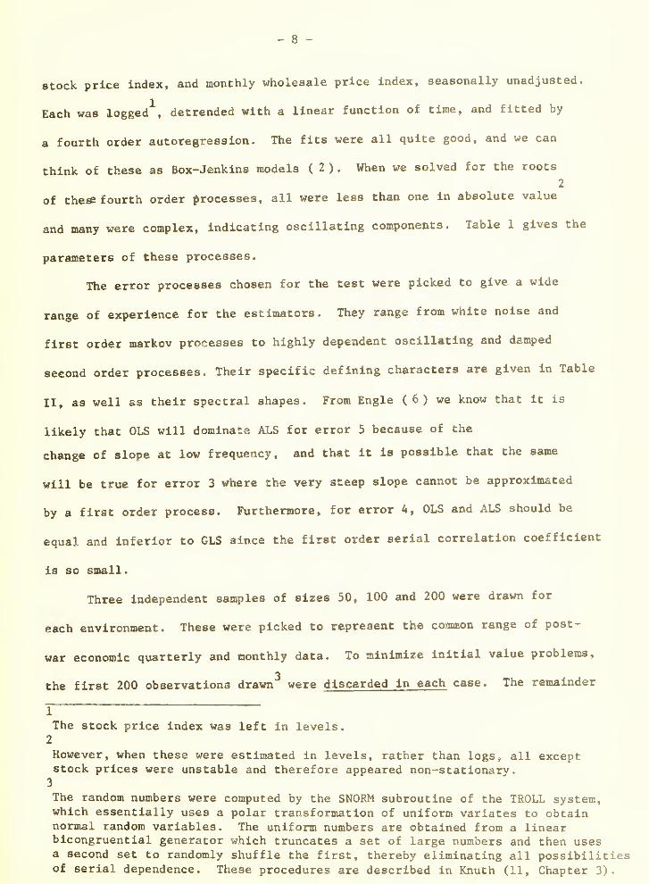
stock price index, and monthly wholesale price index, seasonally unadjusted.

Each was logged , detrended with a linear function of time, and fitted by

a fourth order autoregression. The fits were all quite good, and we can

think of these as Box-Jenkins models ( 2 ) . When we solved for the roots

2

of the* fourth order processes, all were less than one in absolute value

and many were complex, indicating oscillating components. Table 1 gives the

parameters of these processes.

The error processes chosen for the test were picked to give a wide

range of experience for the estimators. They range from white noise and

first order markov processes to highly dependent oscillating and damped

second order processes. Their specific defining characters are given in Table

II, as well as their spectral shapes. From Engle ( 6 ) we know that it is

likely that OLS will dominate ALS for error 5 because of the

change of slope at low frequency, and that it is possible that the same

will be true for error 3 where the very steep slope cannot be approximated

by a first order process. Furthermore, for error 4, OLS and ALS should be

equal and inferior to GLS since the first order serial correlation coefficient

is so small.

Three independent samples of sizes 50, 100 and 200 were drawn for

each environment. These were picked to represent the cosoEon range of post-

war economic quarterly and monthly data. To minimize initial value problems,

the first 200 observations drawn were discarded in each case. The remainder

1

The stock price index was left in levels.2

However, when these were estimated in levels, rather than logs, all exceptstock prices were unstable and therefore appeared non-stationary.

3

The random numbers were computed by the SNORI-1 subroutine of the TROLL system,which essentially uses a polar transformation of uniform variates to obtainnormal random variables. The uniform numbers are obtained from a linearbicongruential generator which truncates a set of large numbers and then usesa second set to randomly shuffle the first, thereby eliminating all possibilitiesof serial dependence. These procedures are described in Knuth (11, Chapter 3).

VARIABLE

- 9 -

TABLE 1

X PROCESSES

2 3 A

(1-YL-YL -yL - y L )X °e12 3 A t t

(1 - a L)(l - a L)(l - a L)(l - a L)X = e

1 2 3 A t t

GNP, Quarterly 1.343 -.182 -.303 .117 .829 .592* .551

PR, Quarterly 1.14A -.186 -.005 -.093 .766* .300*

I, Quarterly, Not .081 .026 -.207 . 7/.0 .966 .918* ,885

Seasonally Adjusted

SP, Monthly 1.200 -.300 .150 -.100 .924 .550 .443*

WPI, Monthly, Not 1.355 -.218 -.142 .004 .975 .667 .214*

Seasonally Adjusted

* A pair of complex roots

- 10 -

TABLE II

ERROR PROCESSES: U

(1 - Y L - Y L )U = (1 - 6 L) (1 - 6 L)U = e1 '2 t 1 2 t t

1 + 661 2

1 - y.

SLOPE (1 - 6^~)^1 6 ) ('-

2 + '-

J )2

(1 - 6^)'' (1 - 6^)

ERROR

1.

11

0.

p_ SLOPE

0.

SPECTRUM

0. .6 0. .6 23.4

3. 1.7 -.72 .8 .988 275,000.

4. .1

1.4

.72

,98

-.8

(.7 + .7i)

,357 2777.0

.707 10.14

- 11 -

were tested for normality and time dependence.

All computation was done on the National Bureau of Economic Research

TROLL time sharing computer system which uses an IBM 360-67 computer. Although

most of the programming is in single precision, the important fast fourier

transform subroutine is calculated in double precision. The estimators are

available for general use through this system.

V. Detailed Results

The choice of an estimator should be made on the grounds of mean

squared error if the investigator has a quadratic loss function. That is,

we should compare the sum of squared bias and variance across estimators.

We found that the bias term was very small and conclude that all the estimators

are essentially unbiased at these sample sizes.

To obtain this result, we computed the ratio of the bias to the

standard deviation of the parameter estimates for each of the 375 environments.

Since each case Is 10 independent observations on a normal (by construction)

paraoieter estimate, this ratio should be distributed as t with 9 degrees

of freedom times root 10 for an unbiased estimator. Only 4 ratios exceeded

the 95% critical value of .715 which is well below the expected 5%. These

all occurred for the estimator HAM 3 and all are negative, however, all

occurred for a sample of 200 observations while for the same environment,

the ratios for smaller samples were quite small and frequently positive.

Furthermore, these were observations with especially small standard

deviations, not large biases. Thus, while it is conceivable that we observe

a bias in HAN 3, it dees not behave like a small sainple bias and we shall

ignore it as random fluctuation.

The error we commit by examining variance throughout the paper

rather than mean squared error is to underestimate the error by one plus

the square of this ratio. Since this is rarely as high as one half, we

are generally making rauch less than a 25% error by ignoring the bias.

- 12 -

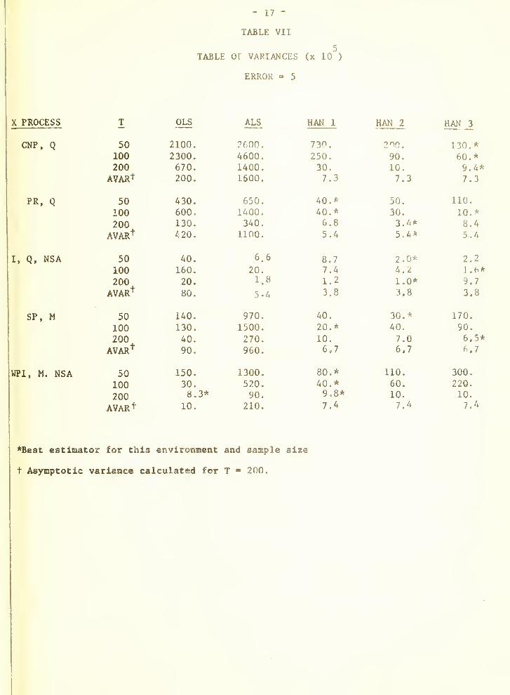
The variances of all the estimators in each environment are given in

Tables III-VII. Each entry is a sample variance of 10 observations and there-

fore the confidence interval associated with any particular number is rather

large. Specifically, the 90% confidence interval covers all values between

one half and two and a half times the estimated value. Most of the interesting

differences between estimators are large and by pooling over environments

we substantially shrink the confidence intervals.

In each case the asymptotic variance for a sample of 200 observations is

presented for comparison. Since the stochastic processes are knovm for each

situation, the asymptotic variance can be calculated by numerical integration

of the relevant spectral density functions.

(12) T AVAR (8 ) ^ 2irI

f (9)de 3 2ir j f (6) f (6) deOLS I J .^ ^ J J -T! ^ "

(13) T AVAR (6 ^ *• o I o^ 1 f (9) f ~^(9) del ,, |f (e)f (e)f (e)de

ALS I y -TT ^ H J ^^ J ,, ^ " u

(14) T AVAR <3 ) « aHAN

As a convention we QormallEe x and u to obtain

(15) ^j \(e)d6 » 1 -J^pJ

""

f^(0)d0 , a^ - 1/4

The spectra of x and u are given by (10) with the appropriate set of y's,

and the spectrum of u, which is the truncated first order approximation.

is given by (10) where n = 1 and y is the true first order serial correlation

coefficient.

Error process 1 is just white noise and therefore all estimators ase

asymptotically equivalent. Notice that for samples of size 50, OLS is

m-in-tmKtn \iar-i ant^a {inA-ifats^i^ h-?r sL.afaf^ for four out of five X orocesses.

- 13 -

TABLE III

TABLE OF VARIANCES (x 10^)

ERROR = 1

X PROCESS T OLS iWLS HAN 1 HAN 2 HAN 3

GNP, Q 50 620. 630.

100 240. 240.

200 160. 160.

AVAR+ 130. 130.

PR, Q 50 1000.* 1100.

100 250. 250.*

200 160. 160.

AVAR+ 130. 130.

I, Q, NSA 50 730.* 790.

100 230. 220.*

200 170. 160.

AVAR+ 130. 130.

SP, M 50 550.* 560.100 170. 160.

200 160, 160.

AVAR"*" 130. 130.

WPI, M, NSA 50 580.* 600.

100 70. 80.

200 90. 90.

AVAR+ 130. 130.

500.* 940. 640.320. 270. 230*120.* 140. 160.130. 130. 130

1100. 1300. 1100.310. 320. 260.

120.* 130. 160.

130. 130. 130.

1100. 920. 760.

250. 310. 240.

120. 120.* 160.

130. 130. 130.

560. 650. 570.

210. 170. 160.*140* 140. 160.

130. 130. 130.

670. 600. 590.

110. 60.* 80.

90, 90.* 90.

130. 130. 130

* Best estimator i6>v this environment and sample else

t Asymptotic variance calculated for T = 200.

- 14 -

TABLE IV

5TABLE OF VARIANCES (x 10 )

ERROR - 2

X PROCESS

GNP» Q

PR, Q

I, Q, NSA

SP, M

WPI, M, NSA

50100200

AVAR

50100200

avar"^

50100200

AVAR"^

50100200

AVAR''

50100200

AVAR

t

OLS

2300.

630.

610410.

2700.

430.490.340.

300.200.

170.

100.

2100.

590.

660.

450.

2100.

420.400.500.

ALS HAN 1 HAN 2 HAN 3

2000. 1800.* 2900. 2000.

590. 750. 570.* 600.

550. 410.* 440. 560.340. 340. 340. 340.

1800.* 2100. 2400. 1900.

390.* 440. 410. 410.

320. 240. 230.* 340.

230. 230. 230. 230.

310. 290.* 290. 290.

150. 200. 160. 140.*

50. 60. 50.* . 50.

50. 50. 50. 50.

1400.* 1500. 1700. 1600.

480. 620. 390.* 430.

580. 510. 500.* 580.

380. 380. 380. 380.

1500. 1900. 1520.* 1700.

310. 420. 180. 210.

430. 420. 450. 440.

490. 490. 490. 490.

* Best estimator for this environment and sample size

t Asjnnptotic variance calculated for T " 200.

l PROCESS

- 15 -

TABLE V

5TABLE OF VARIANCES (x 10 )

ERROR = 3

OLS

GNP, Q 50 4400.100 1600.200 1100.AVARt 1100.

PR, Q 50 2100.

100 1000.

200 500.

AVARt 500.

I, Q, NSA 50 270.

100 540.

200 200.

AVARt 200.

SP, M 50 6200.

100 2300.

200 2200.

AVARt 2100.

WPI, M, NSA 50 flOO.

100 2700.

200 2200.

AVARt 3300.

ALS

40.*40.*20.*

40.

20.*

30.

10.

10.

HAN 1

,6*

,2*

,7

,3

180.*50.*50.*60.

550.*250.*430.*900.

* Best estimator for this environm^ati and sample size

t Asymptotic variance calculated for T = 200.

HAN 2 HAN 3

440. 330. 830.100. 70. 110.190. 40. 60.

10. 10. 10.

220. 110. 110.

60. 40. 10.*50. 20. 8.5*3.9 3.9 3.9

30. 10. 2.17.9 4.7 2.4

1.4 0.6 2.5

2.0 2.0 2.0

1900. 2000. 1700.

250. 220. 290.

260. 220. 130.

20. 20. 20.

4200. 3500. 3300.

750. 690. 740.

960. 1200. 1100.

190. 190. 190.

- 16 -

TABLE VI

5

TABLE OF VARIANCES (x 10 )

ERROR - 4

X PROCESS

GNP, Q

PR, Q

I, Q, NBA

SP, M

WPI, M, NSA

50

100200

AVAR'

50100200

AVAR"*"

50100200

AVAR"*"

50100200

AVAR"*"

50

100200

AVAR"*"

OLS

5400.860.

900.

610.

2300.480.

390.

330.

2000.

590.

290.

300.

3800.

1000.

1300.

1000.

3800.1100.

1100.

1500.

ALS

4300.710430.

520.

2000.

410.

180.

250.

2300.

620.

290.

330.

3600.

1100.

1100.

930.

3700.1100.

1000.

1500.

HAN 1 HAN 2 HAN 3

2 500. 2700. 2200.*320. 360. 260.*310. 270. 240.*180. 180. 180.

1100. 940.* 1400.170. 150.* 190.

120. 100. 100.*90. 90. 90.

1900. 1300. 740.*220. 130. 50.*80. 70. 70.*

50. 50. 50.

2700. 3000. 2600.*500. 380* 380.500.* 490.* 460.*300. 300. 300.

3300. 3000. 3000.*360 410. 350.*840. 730.* 770.

1100. 1100. 1100.

* Best estimator for this environajent and sample size

t Asymptotic variance calculated for T = 200.

- 17 -

TABLE VII

5TABLE or VARIANCES (x 10 )

ERROR =» 5

X PROCESS

GNP, Q

OLS ALS

PR, Q

I, Q, NSA

SP, M

WPI, M. NSA

50100200

AVARI"

50

100200

AVAR''"

50

100200

AVAR"*"

50

100200

AVAR"*"

50100

200AVAR^

2100. 2600.

2300. 4600.670. 1400.200. 1600.

430. 650.

600. 1400.130. 340.

420. 1100.

40. 6.6

160. 20.

20. 1.8

80. 5-4

140. 970.

130. 1500.

40. 270.

90. 960.

150. 1300.

30. 520.8.3* 90.

10. 210.

HAN 1

730.

250.

30.

7.3

40.*40.*6.8

5.4

8.77.41.2

3.8

40.

20.*

10.

6.7

80.*40.*9.8*

7.4

*Best estimator for this environment and sample size

t Asymptotic variance calculated for T « 200.

HAN 2

2'>0,

90.

10.

7.3

50.

30.3.4*5.4*

2.0*4.21.0*3,8

30.*40.

7.06.7

110.

60.

10.

7.4

HAN 3

130.*60.*9.4*7.3

110.

10,

2.2I.e.*

9.7

3.8

170.

90.

6.5*

6.7

300.

220.

10.

7.4

- 18 -

However, the other estimators are very close and for the larger sample

sizes it appears that the optimum estimator is selected randomly. Thus,

both ALS and the spectral estimators appear to have reached their asymptotic

distribution at samples of 100.

Error process 2 is first order markov and therefore ALS is asymptotically

efficient. However, it only captures 3 out of fifteen firsts. Apparently the

three spectral estimators are approaching their asymptotic distribution

Just as rapidly as ALS, and from a comparison of the variances at 200, both

are essentially there.

Error 3 is a strongly dependent process with large positive roots.

Here ALS is a clear favorite as it dominates in 12 situations, in spite

of the fact that the spectral estimators have roughly one third the asymptotic

variance. Because of the steep decline in the spectrum of the errors at the

very crucial low frequencies, we would expect HAN 3 to outperform the other

two versions, and this in fact does happen. Nevertheless, these are all

well above their asymptotic variances. It was in this case that Engle (6)

showed that it would be possible for OLS to be better than ALS, if the

variable was sufficiently concentrated at low frequencies. These results

Indicate that at least for the environments here, this does not happen.

Error 4 has a strong second order dependence but very little first order.

Han 3 is the clear winner and appears to be only slightly above its

asymptotic variance. ALS and OLS do behave very similarly and much worse

than the spectral estimators.

Error 5 has an oscillation with a period of 8 time units. The spectral

estimators take most of the prizes with a slight edge for HAN 3. ALS, as

predicted by Engle, does much worse than OLS.

Overall, the results are very encouraging for the Hannan estimators.

They are generally only slightly above their asymptotic variances over the

range of observations examined, and even in simple situations do as well as the

appropriate estinators. The biggest failure of the spectral estimators

was in error 3 where the difficulty in estimating a steep slope of the

- 19 -

spectrum at low frequencies appeared to generate a large amount of extra

noise In the estimator and enabled ALS to successfully compete at these sample

sizes. HAN 3 was most able to model this behavior but

the choice of n-2 may be in part responsible for this success.

A possible explanation for the failure of HAN 1 and HAN 2 to model the

low frequency peak, is that the bandwidth chosen was too wide to accurately

pick up the peak. Experiments with narrower bandwidths however, lead to

no improvement

.

The simple implications of these results, are that use of one of the

Hannan estimators in place of OLS or ALS will not cost very much for these

sample sizes but will possibly produce a much better estimate.

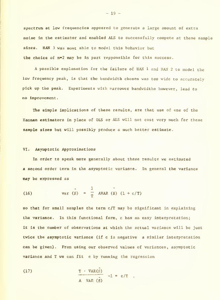
VI. Asjnnptotic Approximations

In order to speak more generally about these results we estimated

a second order term in the asymptotic variance. In general the variance

may be expressed as

1

(16) var (6) " ~ AVAR (B) (1 + c/T)

so that for small saniples the term c/T may be significant in explaining

the variance. In this functional form, c has an easy interpretation;

it is the number of observations at which the actual variance will be just

twice the asymptotic variance (if c is negative a similar interpretation

can be given). From using our observed values of variances, asymptotic

variance and T we can fit c by running the regression

(17) T • VAR(p)

T -1 - c/T .

A VAR ($)

- 20 -

TABLE VIII

COEFFICIENTS AND T-STATISTICS

(T*VAR/AVAR) -1 => c /T

ERROR ESTIMATOR

OLS ALS HAN 1 HAN 2 HAN 3

1. 12.76 14.65 20.52 26.97 14.69

(1.72) (1.88) (2.53) (2.88) (1.91)

2. 8.57 14.42 18.93 22.47 15.41

(.97) (1.59) (2.08) (1.99) (1.66)

3. -14.89 -15.10 929.53 601.80 325.20(-2.77) (-1.18 (5.11) (4.15) (4.85)

4. 11.57 10.32 109.92 91.40 48.72

- (1.16) (1.05) (2.81) (3.24) (2.81)

5. 25.25 -18.16 368.70 143.99 268.23

(.81) (-1.51) (2.88) (3.77) (3.74)

TABLE IX

POOLED REGRESSIONS

COEFFICIENTS WITH T-STATISTICS

T*VARDEPENDENT VARIABLE:

AVAR_ -1

VARIABLE OLS ALS HAN 1 HAN 2 HAN 3

1/T 8.65(1.24)

1.23

. (.25)

127.53(2.43)

69.81(2.05)

86.25(3.41)

ERROR SLOPE/T .003(6.84)

.002(6.97)

.00087

(4.21)

- 21 -

There Is of course a serious question as to whether we can pool over x

processes or error processes. We felt that pooling over x processes was

not only legitimate but desirable since we would like to Interpret our results

In terms of a typical economic process.

We first estimated c for each estimator and error. These are presented

in Table VIII along with the t-statistics. Notice that the values

for c are generally not significantly different from zero for OLS and ALS

and in fact are often negative suggesting that they do better than their

asymptotic variances. The spectral estimators however, all have strongly

positive and generally significant coefficients. Because the sizes differed

so much, we decided that it was necessary to make an effort also to explain

the differences between the errors.

In the light of the difficulties discussed in estimating the spectrum

at low frequencies, we hypothesized that the steepness of the spectrum

at lov frequencies might be an important variable explaining how the spectral

estimators behaved in different environments. The slope of the spectrum

at zero frequency is zero, but at low frequencies it is proportional

to the negative sine. The absolute value of the proportionality constant is

(18J SLOPE- |a^/(l-aj^) +(1^/(1-^2^ \ I il-<x^'^ iX-^^

where o's are the roots of the error process.

For the spectral estimators the pooled equation was

T • VAR(6)

(19) X— - 1 = c/T + c SLOPE/T

A VAR (6)

- 22 -

Alternative forms used the first order serial correlation coefficient

or a variety of functions of the asymptotic variances. This variable

proved the best but a great deal of the variance remains unexplained and a

finite sample theory would provide a better equation for this estimation.

Equation (17) was estimated for OLS and ALS over the entire set of

75 observations. The validity of the pooling assumption in each case was

tested. Both OLS and ALS passed easily. Upon pooling, we found the

coefficients are small, positive and insignificant.

The aggregation test was passed easily by HAN 1 and HAN 2 and only

failed by a small margin for HAN 3. Therefore we pooled this data and

estimated (19) . The results in Table IX indicate that the slope variable

is very significant and that the coefficient of reciprocal sample size

is also significant although with a large standard error. Unless the slope

is very great, HAN 2 and HAN 3 should be less than twice, and HAN 1 slightly

more than twice the asymptotic variance at a sample size of 100. HAN2

appears to be the best on these grounds > reaching this point by T»70. However,

in the presence of an ill-behaved error process with a steep low frequency

spectrum, HAN 3 would be superior since the slope coefficient is less than

half that for HAN 2. The estimator HAN 1 is dominated on both counts bv the

other two versions

.

For none of these equations in either the original or pooled form could we

reject at a 95% level, the hypothesis that the constant term is truely

zero as indicated by the asymptotic theory. This provides some evidence for

our estimating equations.

I

- 23 -

VII. Conclusions

We draw the following six conclusions from this study:

(1) We have formulated and programmed a computationally simple Hannan

estimator which gives reasonable results. It is not iterative and is there-

fore not expensive to compute. Three versions which differ only for finite

samples are examined.

(2) Based on the pooled results of five typical x-processes and five

error processes, we find that our Hannan estimator will be approximately

2 times its asymptotic variance at sample size 100, provided the slope of

the spectrum near is not large. Under the traditional assumptions about

error processes, the estimators reach this point for samples of size 20.

v,J) On these same x- and error processes, we find no significant trend for

ALS or OLS in terms of asymptotic variance.

(4) Thus, we expect that if the Hannan estimator's asymptotic variance is

no more than half of that of OLS or ALS, then it will pay to switch to the

Hannan estimator at sample size 100. This Is the trade-off we observe

between robustness and finite sample properties of the Hannan estimator.

(5) There are some principles of choice among the Hannan estimators. HAN 2

(piecewise constant disturbance spectrum) appears to dominate HAN 3 (auto-

regressive error process) as long as the slope of the error spectrum near

zero is not large; otherwise this judgement is reversed. HAN 1 (rectangular

moving average of residual periodogram) is dominated by the other two.

(6) Even at sample size 50, there appears to be no significant bias in any

of the environments for any of the estimators •

- 2A -

BIBLIOGRAPHY

(1) Amemlya, Takeshi, "Generalized Least Squares with an Estimated AutocovarlanceMatrix", forthcoming in Econometrtca .

(2) Box, George E.P., and Gwllym M. Jenkins, Time Series Analysis, Forecasting, andControl , Holden Day, 1970.

'

(3) Cooper, Phillip J., "Asymptotic Covarlance Matrix of Procedures for LinearRegression in the Presence of First Order Serially CorrelatedDisturbances", Ecgnometrica , (March 1972), 305-310.

(4) Duncan, D.B. and R. Jones, "Multiple Regression with Stationary Errors,"American Statistical Association Journal , Vol 6 (December, 1966),917-928.

(5) Engle, Robert F. , "Band Spectrum Regression," InternationalEconomic Review , February 1974,

(6) Engle, Robert F., "Specification of the Disturbance for Efficient Estimation",Econometrica , forthcoming.

(7) Granger, C.W.J. , "The Typical Spectral Shape of an Economic Variable,"Econometrica . 34 (1966), p. 150.

(8) Griliches, Zvi and Rao, P., "Small-Sample Properties of Several Tv70-

Stage Regression Methods in the Context of Autocorrelated Errors",Journal of American Statistical Association, 64 (1969) 253.

(9) Hannan, E.J., Multiple Time Series , New York, John Wiley, 1970.

(10) Hannan, E.J., "Regression for Time Series," in Time Series Analysis ,

ed. by M. Rosenblatt, New York, John Wiley, 1963, 14-37.

(11) Knuth, Donald E., The Art of Computer Programming, Vol II - Seminumerlcal

Algorithm, Addision Wesley, 1969.

(12) Maddala, G.S. "Generalized Least Squares with an Estimated VarianceCovarlance Matrix", Econometrica , January 1971.

(13) Parzen, E., "Multiple lime Series Modeling", in Multivariate Analysis ,

Academic Press, 1969.

(14) Watson, G.S. and E.J. Hannan, "Serial Correlation in Regression Analysis II,"Biometrika 43 (1956), 436-448.

Date Due

tfB»^-^tffi 1 7 '^,

K-KQV 5 Ti: i

MAR 5 It ^

jWi-**-^*^:!iY13'BB

OEC 1 7 'IS

MAR 2 2 71

flE 2 8 ^OQ;

AU6 3t 78

MAT 3 2 T^

•^

) Lib-26-67

Mil 1 lllKAItlLS

3 TDfiO DD3 TbD ETfl

3 TDflD D03 TbO 314MIT LlBRAHItS

3 TDflD D 3 ^bD 33 D^

3 TDflD DD3 TbO 3SS

3 TDfl

MIT LIBRARIF'^

DlilliJlllllliliilli

3 TET ET3MIT LIBRARIES

3 TDflD DD3 TET 3n

3 TDflD D03 TET 33SMIT LIBRARIES

3 TOfiO DD3 TET 35