Some comments on the TLM modellingof acoustic Doppler effect

R.V. Aldridge1, D. de Cogan1*, M. Morton1, W. O'Connor2 and V. Sant1

AbstractThis paper discusses some anomalies that are observed innumerical treatments of Doppler processes. The situationcan be significantly improved by the use of distributedsources, but the real problem lies with the failure of meshdispersion to cancel in the case of moving sources. Atechnique for the cancellation of these effects appears toeliminate the problem.

IntroductionThe Doppler effect in acoustics is well studied analytically and students of physics aretaught to distinguish between moving source and/or moving observer. It is therefore quitestrange that there seems to be relatively little evidence of work on the numericalmodelling of this phenomenon. Recently, several groups who are developing numericalalgorithms involving the Transmission Line Matrix (TLM) modelling technique haveencountered problems when considering moving sources and these are summarised in thispaper.

TLM is a form of time-domain numerical modelling which was first developed to treatproblems in electromagnetics and microwaves. It has already been used to model a rangeof acoustic problems. Saleh and Blanchfield [1] demonstrated that the polar plots due tophased transmitters were identical to the analytical results. Orme et al [2] investigatedthe possibilities of acoustic imaging based on data provided by TLM propagationmodels. Willison's work on submarine acoustic propagation [3] was hampered by thelack of open-boundary descriptions and smooth (non-stepped) boundary definitions.Pomeroy [4] has developed a smooth boundary algorithm and has demonstrated how itimproves the pressure response in the Buckingham and Tolstoy [5] bench-mark test.O'Connor has used TLM to investigate air-membrane interactions which include theeffects of the viscosity of the medium and has applied this in a practical head-phonemodel [6].

1 School of Information Systems, University of East Anglia, Norwich NR4 7TJ (UK)* To whom any correspondence should be addressed (ddc@sys.uea.ac.uk)2 Department of Mechanical Engineering, University College Dublin, Belfield, Dublin 4 (Ireland)

It is believed that the difficulties which have been encountered when treating acousticproblems which involve movement are due to a variety of factors including the simplisticmanner in which TLM modellers tend to define sound sources. This paper has acautionary element intended to help those who may wish to apply this technique toproblems with moving sources and/or observers. We will start by providing a briefoutline of the TLM method. This will be followed by an enumeration of the problemsthat have been encountered with Doppler simulations. We will demonstrate the benefitsof a distributed source and conclude with a discussion of the source of the real problem,namely dispersion effects.

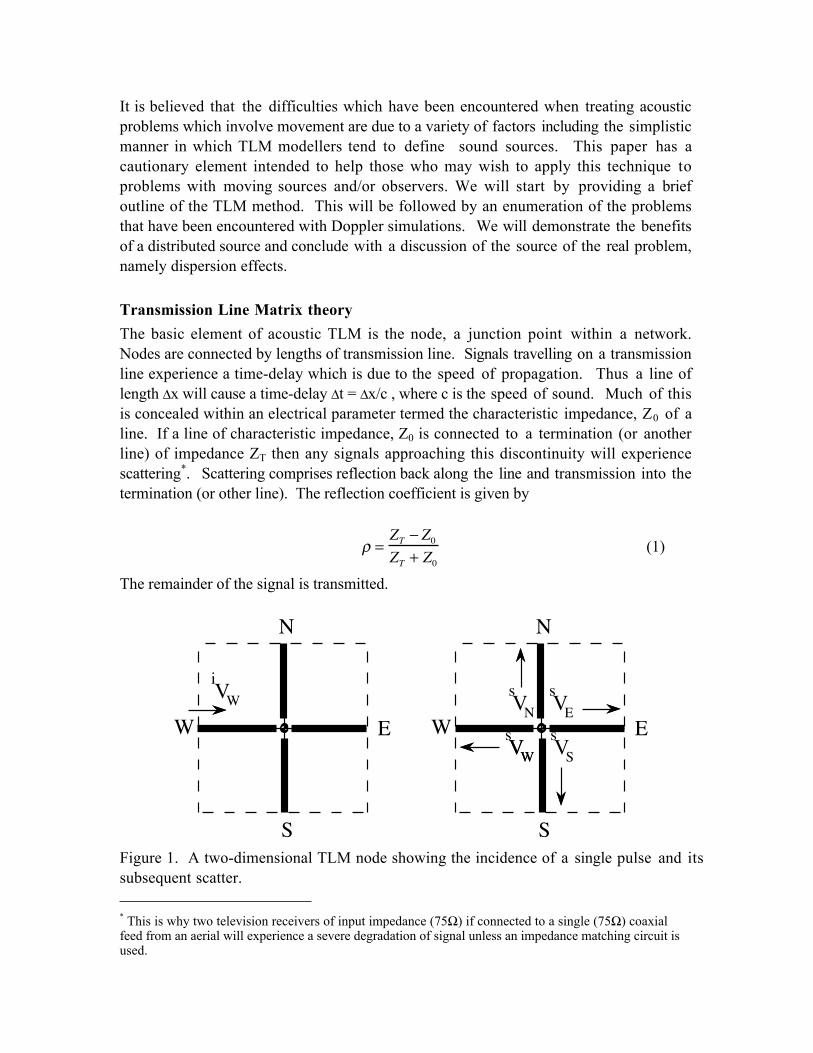
Transmission Line Matrix theoryThe basic element of acoustic TLM is the node, a junction point within a network.Nodes are connected by lengths of transmission line. Signals travelling on a transmissionline experience a time-delay which is due to the speed of propagation. Thus a line oflength Δx will cause a time-delay Δt = Δx/c , where c is the speed of sound. Much of thisis concealed within an electrical parameter termed the characteristic impedance, Z0 of aline. If a line of characteristic impedance, Z0 is connected to a termination (or anotherline) of impedance ZT then any signals approaching this discontinuity will experiencescattering*. Scattering comprises reflection back along the line and transmission into thetermination (or other line). The reflection coefficient is given by

ρ =ZT − Z0ZT + Z0

(1)

The remainder of the signal is transmitted.

N

S

EWVi W

N

S

EWVs N Vs E

Vs SVs WVW

Figure 1. A two-dimensional TLM node showing the incidence of a single pulse and itssubsequent scatter. * This is why two television receivers of input impedance (75Ω) if connected to a single (75Ω) coaxialfeed from an aerial will experience a severe degradation of signal unless an impedance matching circuit isused.

Figure 1 shows an example of a scattering process in two dimensions. In this case the noderepresents the intersection of two two-wire transmission lines. If we use the points of acompass to indicate direction with respect to the node then a signal is seen to be incidentfrom the west. TLM assumes that individual signals are represented by impulses so thateach can be treated independently of other pulses at a single position in space. Any wave-form is then represented by a modulated train of impulses each separated by thediscretisation time, Δt. Based on this assumption we can say that the signal is unaware ofanything but its immediate surrounds until the precise instant when it arrives at the node.It then sees three other lines in front of it, which, so far as it is concerned, appear to be ofinfinite length. It sees this assembly as three lines in parallel, which is equivalent to asingle line of impedance Z0/3. This can be inserted into eqn (1) to obtain a value ρ = -1/2,the magnitude of the signal which is scattered back along the west line. Since thetransmitted signal goes equally into each of the other lines we can write ρ +3τ = 1, fromwhich we obtain τ = 1/2.

This can be extended so that the relationship between the magnitudes scattered to North,South, East and West can be related to the magnitudes incident from North, South, Eastand West for each location (x,y) and expressed in matrix form as

s MN

MS

ME

MW

⎡

⎣

⎢ ⎢ ⎢ ⎢ ⎢

⎤

⎦

⎥ ⎥ ⎥ ⎥ ⎥

= S[ ]

i MN

MS

ME

MW

⎡

⎣

⎢ ⎢ ⎢ ⎢ ⎢

⎤

⎦

⎥ ⎥ ⎥ ⎥ ⎥

(2)

where S[ ] =12

−1 1 1 11 −1 1 11 1 −1 11 1 1 −1

⎡

⎣

⎢ ⎢ ⎢ ⎢ ⎢

⎤

⎦

⎥ ⎥ ⎥ ⎥ ⎥

is the scattering matrix.

Signals which are scattered according to eqn (2) become incident on nearest neighbours atthe next time-step. This 'connection' process can be centred on the node (x,y) and thisresults in a set of connection equations relating the magnitudes incident at iteration step,(k+1) with the magnitudes scattered at step, k.

k +1iMN (x,y)=k

sMS (x,y +1)

k +1iMS (x,y)=k

sMN (x,y −1)

k +1iME(x,y)=k

sMW(x +1,y)

k +1iMW(x,y)=k

sME(x −1,y)

(3)

Equations (2) and (3) provide a general set of equations which can be applied to two-dimensional scattering problems.

We next draw an analogy between electricity and acoustic propagation where we interpretinstantaneous pressure as being equivalent to voltage and current as being equivalent todisplacement. The voltage (pressure) at node (x,y) is given by the sum of all incidentcurrents divided by the sum of all line admittances (admittance is the reciprocal ofimpedance) [7]. For a two dimensional model this yields

k +1φ(x,y) =1

2 k +1iVN + k +1

iVS + k +1iVE+ k +1

iVW[ ] (4)

where k +1iVN , k +1

iVS , k +1iVE and k +1

iVW are the voltage magnitudes of the impulse signals ineqns (2) and (3).

Figure 2 Results by Jaycocks and Pomeroy [9] for an acoustically reflecting closed-surface in the form of a projectile which moves one node per iteration.

Moving sources in TLMWork by Pomeroy on surface conforming boundaries seems to have drawn inspirationfrom an open suggestion by Wolfgang Hoefer at the 1995 International TLM Workshopin Victoria, British Columbia. This used ideas for treating moving boundaries which hadbeen developed by Beyer [8]. Pomeroy demonstrated an impressive two-dimensionalexample of acoustic reflection from a bullet-like projectile, moving at one unit distance inone time-step [9] which is shown in figure 2. It must however be realised that this is infact an example of trans-sonic motion (Mach 1.414), since the speed of sound on a TLMmesh is c0/√2 [7]. Close inspection of the picture also shows evidence of signaldispersion.

Figure 3. Behaviour of a TLM modelled moving source showing spurious bow-wave.

Sant [10] encountered problems when attempting to model a single-point moving sourcein a two-dimensional space. The first method for modelling motion at U = Vsound/N wasto move the source by one unit distance after every N time-steps. This resulted in strongdispersion with a very pronounced effect rather like the bow-wave left by a ship as ittravels through water. The next method that was adopted was to use N sub-meshes,where each submesh was displaced from the next by 1/N of the unit spatialdiscretisation. At the first time-step the source was placed on the first sub-mesh. It wasthen moved to the second submesh for the next time-step, so that after n time-steps ithad moved in a continuous step-wise fashion through one unit distance. The signalpropagated independently on each sub-mesh and the resultant at any time was thesuperposition of all n sub-meshes. This gave some improvement but did not eliminatethe problem. The next method that was investigated was a distributed source based onan original suggestion by O'Connor [11]. As a signal moves between nodes x and x+1 itis distributed over both and a weighted mean is taken. Thus, if it is currently located onethird of the way between these two points then it represents (2/3)*V(x) + (1/3)*V(x+1).It was also possible to extend this technique so that any two-dimensional motion couldbe represented as the weighted mean of the four surrounding points. This was found togive a significant improvement, particularly in relation to the level of dispersion that wasobserved.

0 1 2 3 4 5 6 7 8 9 10-15

-10

-5

0

5

10

N, the source velocity in terms of the free-space sound velocity (Us = V/N)

Figure 4. Experimental plots of ±f/Δf vs N obtained by Sant [10] shown as 'o' (advancingsource), 'x' (retreating source) compared with the equivalent analytical results (dashedlines)

In addition to a residual bow-wave (figure 3) which was present in all except slow-moving sources, there were two other anomalies which Sant observed. The first was thelack of agreement between physical theory and numerical experiment. The theory of theDoppler effect for a moving source predicts the relationship between relative change offrequency source velocity for movement towards the observer

Δff =

US

V −US (5)

in the case where source velocity is defined in terms of the sound velocity (Us = V/N) wehave

Δff =

1N −1 (6)

The equivalent result for movement away from the observer is−Δff =

1N +1 (7)

Attempts by Sant [10] to model a moving source using the techniques outlined aboveyielded relative frequency shifts which are compared with those predicted by eqns (6)and (7) and are shown in figure 4.

These attempts to compare TLM-derived results with eqns (6) and (7) overlooked thefact that the velocity of a signal on a two-dimensional mesh, Vm is equal to V/(√2),

where V is the free-space velocity. Thus when the velocity of the observer on the meshis defined as Vm /N, then eqns (2) and (3) become

and

(8)

for the advancing and retreating sources respectively. When the equations in (8) weretested using a series of TLM simulations, then the agreement between theory andexperiment was exact within the limits of error of the FFT routine (figure 5). Thisconsideration also applies after appropriate reformulation to the case of an observermoving with respect to a stationary source.

0 2 4 6 8 10 12 14 16 18 20-25

-20

-15

-10

-5

0

5

10

15

20

25

Figure 5. A comparison between theory and experimental Doppler shifts as a function offractional Mach number, N (horizontal axis) for a moving observer. The vertical axis is±f/Δf for the theoretical results (solid lines) and ±(√2)f/Δf for the numerical results,shown as data points (stars = advancing, circles = retreating). The dashed lines indicatethe error limits which arise from the frequency discretisation in the FFT output.

Spurious harmonicsThe appearance of spurious harmonics was another anomaly was observed. Amplitude-time samples were collected during approach towards or departure from a stationaryobserver. These were subjected to a fast Fourier transform (FFT) which yielded anamplitude-frequency spectrum. In addition to a frequency shifted fundamental therewere a series of harmonics and these seemed to appear in pairs (figure 6). Similar

observations were reported by other researchers at the 1999 International TLMWorkshop at the University of Nice Sophia Antipolis, France [12, 13, 14].

0 0.05 0.1 0.15 0.2 0.25 0.3 0.35 0.4 0.45 0.50

0.1

0.2

0.3

0.4

0.5

0.6

0.7

0.8

0.9

1

Figure 6. Main peak and spurious harmonics in the Fourier results obtained by Sant [10]for a moving source retreating at V/5 (the axes represent normalised amplitude andfrequency).

Source descriptions and distributed excitationsInitially it was believed that these observations were partly due to the nature of thedescription of the moving sinusoidal source.

20 40 60 80 100 120

-0.8

-0.6

-0.4

-0.2

0

0.2

0.4

0.6

0.8

nodal position

Figure 7. Symmetric sinusoidal generation from a point source.

The standard method of defining a single point sinusoidal source in TLM is most clearlypresented in one dimension as a stationary excitation that transmits equal amplitude toleft and right. Although (x = 60) in figure 7 may provide a point of reflective symmetryit does not represent the super-position of left and right-going pulses of equal phase andmagnitude.

TLM Modellers frequently excite in space or in time, but seldom both simultaneously, asit adds to the complexity of the algorithm. We decided to investigate the effects ofspace/time excitation and used a region within our mesh where we distributed oursinusoidal excitation within a two-dimensional Gaussian envelope, rather like thefundamental mode of a square drum-skin. Although the spurious harmonics were noteliminated, they were significantly suppressed. This led us towards a new concept,namely the cancellation of dispersion effects.

The effects of mesh dispersion on moving sourcesTime domain samples were collected for observers before and behind a single pointsinusoidal source moving at different velocities. The frequency spectra derived fromFFT indicated that in addition to the velocity-determined frequency shift, there was aseries of harmonics which were present in both the approaching and receding samples,but were particularly prominent in the region enclosed by the 'bow-wave'. Similarobservations have been reported by other researchers [2, 3, 4]. It is our belief that thiseffect is due to mesh dispersion which is unbalanced due to source motion. Todemonstrate this we should recall that if a single-shot excitation is injected into a two-dimensional TLM mesh then the resultant propagation exhibits dispersion (figure 8).

Figure 8 Dispersion in a 2D mesh following the injection of a single-shot initial excitation.

This is not normally observed when stationary sinusoidal excitations with λ ≥ 10Δx areused. However, if the sinusoid is moved, even at relatively low velocities, then additionalharmonics can be observed, particularly on the receding signal (figure 9a). Now, if the

moving sinusoid is distributed over two or more adjacent sites (i.e. not a point source),then the high-frequency components should cancel each other. Figure 9b shows the sameproblem with four adjacent identical sinusoidal sources (λ = 30Δx) moving in-line.

0 50 100 150 200 250 300-3

-2

-1

0

1

2

3

position

Figure 9a. Time-domain response along the track of the central point of a 41 node widesinusoidal line-source (λ = 30Δx), initially lying along (x = 100), which is moved one nodeto the right every 5 time-steps in a 300×300 node-space surrounded by perfectlymatched absorbers.

0 50 100 150 200 250 300-10

-8

-6

-4

-2

0

2

4

6

8

10

Figure 9b. The same problem with identical line sources lying along (x =100,101,102,103)

This non-cancellation of dispersion is exhibited with even simpler excitation. Nodispersion is evident when a constant unit source is injected at a fixed point on a two-

dimensional TLM mesh. If, however, this source is moved, then oscillatory componentsare observed. A time-domain signal along the line of movement of such a source exhibitsfour features: some advancing oscillation, a positive peak followed by a negative peakwith strong trailing oscillations. A bipolar distributed source with +1 and -1 separatedby 2Δx was found to inhibit the negative peak, while retaining the essential oscillatoryfeatures. Figure 10 shows the frequency spectrum for such a bipolar source moving atone fifth of the free-space propagation velocity. The position of the dominant harmonicin the retreating signal was found to move to lower frequencies at lower source velocities.

0 500 1000 15000

0.2

0.4

0.6

0.8

1

1.2

1.4 x 10-3

amplitude

advancing towards observer

retreating from observer

Figure 10. Frequency response for two unit valued sources, +1 initially at (100,150) and-1 initially at (98,150), which are moved one node to the right every 5 time-steps in a300×300 node-space surrounded by perfectly matched absorbers. The results are basedon 256 time-samples where the dotted line shows the spectrum for a source advancingtowards an observer and the solid line is for the source retreating from an observer.

Bow-wave angleCareful observations show that TLM simulations of an isolated moving source exhibittwo 'bow-waves'. The retreating envelope is less than 90º and encloses the mostprominent region of harmonics. However, there is also an advancing envelope which isgreater than 90º. Both of these can be interpreted in terms of dispersive effects. Thedispersion pattern following a single-shot injection into a two-dimensional mesh exhibitsregions of minimum dispersion at 45º to the mesh axis centred on the injection point. So,if a continuous unit source injects at (x,y) at the start of the simulation then its dispersivewave-front will have moved a distance NΔx/√2 in time NΔt. At this time the source willhave moved a distance Δx and will be centred on (x+1,y). The signal emitted at thisinstant will travel dispersively with minima at 45º centred on where the source is now. If

the simulation is run for some time, then the angles between the source in its currentposition and all previous dispersive minima are:

for the advancing signal (5)

for the retreating signal (6)

These expressions have been confirmed in experimental simulations between V/4 andV/10.

ConclusionsIn this paper we have discussed the various anomalies that have been observed whenusing TLM to model moving sources and have provided reasonable explanations as totheir origins. Although developed for acoustics, it is believed that the same considerationsapply in electromagnetics. Indeed, it is believed that they also apply in any other time-domain techniques that display mesh dispersion. The problem of spurious harmonicgeneration can be eliminated by smearing the source over several adjacent nodes.

References1. A.H.M. Saleh and P. Blanchfield, Analysis of acoustic radiation patterns of array

transducers using the TLM method, Int. J. Numerical. Modelling 3 (1990) 39 - 56

2. E. A. Orme, P.B. Johns and J.M. Arnold, A Hybrid modelling technique forunderwater acoustic scattering, Inter. Jour. Of Numerical Modelling, 1 (1988)189-206

3. P. A. Willison, Transmission Line Matrix modelling of underwater acousticpropagation, Ph.D. Thesis, UEA, Norwich (1992)

4. R. Jaycocks, S. C. Pomeroy, A method for superposition for the precise placementof arbitrary or moving boundaries within a TLM mesh, in Digest 1st Int. Workshopon TLM Theory and Applications (Victoria, BC, Canada) 269-272, August 1995

5. M.D. Melton, J. R. Flint, S. C. Pomeroy, D. D. Ward Numerical results of aprecise placement algorithm for TLM, Proc. 3rd Int. Workshop on TransmissionLine Matrix (TLM) and it’s applications, Université de Nice Sophia, Antipolis,Oct 1999, 215 - 221

6. W. O'Connor, TLM modelling of devices with acoustic mechanical coupling "TLMApplications Beyond Electromagnetics" Proceedings of an informal meeting held atthe University of Hull (24 June 1997), School of Information Systems (UEA),Norwich, 1997 (ISBN 1 898290 06 7), pp 2.1 - 2.8

7. C. Christopoulos, The transmission-line modelling method TLM, The IEEE/OUPSeries, IEEE press (1995) ISBN (0-19-856533-X)

8. U. Müller, A. Beyer and W.J.R. Hoefer, Moving boundaries in 2-D and 3-D TLMsimulations realised by recursive formulas IEEE Trans. MTT-40 (1992) 2267 -2271

9. R. Jaycocks and S.C. Pomeroy The precise placement of boundaries within a TLMmesh with applications "TLM: The wider applications" Proceedings of an informalmeeting held at the University of East Anglia, Norwich (27 June 1996), School ofInformation Systems (UEA), Norwich, 1996 (ISBN 1 898290 01 6), pp 2.1 - 2.5

10. V. Sant Transmission Line Matrix (TLM) modelling of Doppler effect MSc thesis,University of East Anglia, Norwich 1999

11. W. O'Connor (private communication)

12. W. O'Connor, Waves in moving media using TLM Proceedings of ThirdInternational Workshop on Transmission Line Matrix (TLM) Modelling, Theoryand Applications, University of Nice-Sophia Antipolis, 27 - 29 October 1999,pp281 - 284

13. J. Represa, An improvement of the Doppler effect simulation using scalar TLMProceedings of Third International Workshop on Transmission Line Matrix (TLM)Modelling, Theory and Applications, University of Nice-Sophia Antipolis, 27 - 29October 1999, pp 159 - 166

14. J.A. Porti and J. Morente, TLM method and acoustics Proceedings of ThirdInternational Workshop on Transmission Line Matrix (TLM) Modelling, Theoryand Applications, University of Nice-Sophia Antipolis, 27 - 29 October 1999, pp135 - 143