Ann Oper Res (2010) 181: 443–462DOI 10.1007/s10479-010-0757-3

Solving the Rectangular assignment problemand applications

J. Bijsterbosch · A. Volgenant

Published online: 5 June 2010© The Author(s) 2010. This article is published with open access at Springerlink.com

Abstract The rectangular assignment problem is a generalization of the linear assignmentproblem (LAP): one wants to assign a number of persons to a smaller number of jobs, min-imizing the total corresponding costs. Applications are, e.g., in the fields of object recogni-tion and scheduling. Further, we show how it can be used to solve variants of the LAP, suchas the k-cardinality LAP and the LAP with outsourcing by transformation. We introduce atransformation to solve the machine replacement LAP.

We describe improvements of a LAP-algorithm for the rectangular problem, in generaland slightly adapted for these variants, based on the structure of the corresponding costmatrices. For these problem instances, we compared the best special codes from literatureto our codes, which are more general and easier to implement. The improvements lead tomore efficient and robust codes, making them competitive on all problem instances and oftenshowing much shorter computing times.

Keywords Linear assignment · k-Cardinality linear assignment · Linear assignmentproblem with outsourcing · Machine replacement

1 Introduction

The linear assignment problem (LAP), also denoted as the weighted bipartite matchingproblem, is well known and intensively studied. It is defined on two equally sized node setsN1 and N2, and a set of feasible assignments A = {(i, j)|i ∈ N1, j ∈ N2}, where each arc(i, j) ∈ A has a cost cij . The objective is to assign each node in N1 to exactly one node in N2,such that the total cost is minimized. For convenience we refer to nodes in N1 as personsand in N2 as jobs; we denote |N1| as n1 and |N2| as n2. Allowing n1 �= n2, say n1 < n2,is a generalization of the LAP known as the rectangular LAP (RLAP). With the binary

J. Bijsterbosch · A. Volgenant (�)Operations Research Group, Faculty of Economics and Econometrics, University of Amsterdam,Roetersstraat 11, 1018 WB Amsterdam, The Netherlandse-mail: a.volgenant@uva.nl

444 Ann Oper Res (2010) 181: 443–462

variables: xij = 1, if person i is assigned to job j and 0 otherwise, and the correspondingcosts cij the RLAP can be stated as

(RLAP) min∑

i∈N1

∑j∈N2

cij xij

subject to∑

j∈N2xij = 1, i ∈ N1

∑i∈N1

xij ≤ 1, j ∈ N2

xij ∈ {0,1}, (i, j) ∈ A

and the corresponding dual problem with the dual variables or node potentials ui and vj as:

(DRLAP) max∑

i∈N1ui + ∑

j∈N2vj

subject to cij − ui − vj ≥ 0, (i, j) ∈ A

vj ≤ 0, j ∈ N2

To solve the RLAP by extending it to a (square) LAP by adding dummy variables is wellknown and goes back to Egervary and Konig, see, e.g., Burkard et al. (2009) for furtherreading on this issue. The transformation increases the computational time by increasingthe size of the problem and introduces degeneration into it, i. e., each optimal solution ofthe original problem instance corresponds generally to (n2 − n1)! optimal solutions of theextended instance. Hence LAP algorithms have been modified for rectangularity—see, e. g.,Bertsekas et al. (1993) or Volgenant (1996).

(R)LAP is a relaxation of problems as the traveling salesman, the quadratic assignmentand vehicle routing. Application fields are, e.g., 1. scheduling and 2. object recognition.

1. Scheduling: Mosheiov and Yovel (2006) formulates the single machine problem with unitprocessing times as an RLAP that minimizes the sum of the earliness and tardiness costs.

Pinedo (2002) considers parallel scheduling to minimize the sum of the flow times ofall jobs, e.g., programs on computer processors. Let n jobs to be processed on one of m

machines, with pij the time to process job i on machine j . The flow time of all the jobsassigned to machine j is found by multiplying the processing times, of the last job by1, of the second last job by 2, etc., and then by summing these values. One can assign ajob i in n × m ways, to one of the machines and to one of the kth to last positions on themachine, with cost cij = kpij . Thus the problem is an RLAP of size n × nm.

2. Object recognition: We mention two applications:Handwriting recognition: In (Chinese) handwriting, each character can be viewed as

a set of, line segments to be used in a similarity measure between an unknown inputcharacter and a reference character, to find an optimal matching among their sets of linesegments, say �1 and �2. By comparing the input character to all reference characters,it is recognized as the one with the highest similarity (or lowest cost) if this similarityexceeds a given threshold, and rejected otherwise. The problem to find an optimal matchreduces to a LAP, see Hsieh et al. (1995), with the cost of assigning line segments i ∈ �1

and j ∈ �2, depending, e.g., on their lengths and their angles. The problem is an RLAPif |�1| �= |�2|.

Multi-object tracking in air traffic control or radar tracking, links targets with tracks.One can partition sensor observations into tracks in some optimal way, to accuratelyestimate the real tracks. Two sensors located at different sites provide each a line anobject must lie on; the intersection of the two lines determines the location of the objectin 3-dimensional space. To locate the objects in time, each sensor provides a set of lines.

Ann Oper Res (2010) 181: 443–462 445

Taking measurements at distinct times, the new sensor measurements, the targets, mustbe matched with the predicted positions of the existing tracks. Due to false alarms, misseddetections and inaccuracy some measurements cannot be matched to (say n2) targets, seeBertsekas and Castañon (1992). With say n1(< n2) remaining measurements, one cansolve the problem as an RLAP of size n1 × n2.

The following LAP variations can be solved by transforming them to an RLAP:

• k-LAP, i.e., the k-cardinality LAP, see Dell’Amico and Martello (1997), defined for agiven positive integer k (k ≤ n), is the problem to assign only k (out of n) persons to k

(out of n) jobs, minimizing the total cost.• LAPout, i.e., the LAP with outsourcing, see Wiel Vander and Sahinidis (1997), a problem

with the extra possibility that each ‘internal’ person can either be assigned to an available‘internal’ job or outsourced to an ‘external’ job. Similarly, each internal job can either beassigned to an available internal person or outsourced to an external person.

We introduce a transformation to solve

• k-LAPrep, i.e., the problem of replacing (at most) k machines, see Caseau and Laburthe(2000). Suppose the manager of a plant has the funds to replace k of the available ma-chines by newer ones; then k-LAPrep is the problem to optimally replace k machines aswell as to assign tasks to machines under minimal production cost.

Volgenant (1996) has adapted LAPJV to solve the RLAP; we denote this algorithm asRJV: rectangular LAPJV. It is based on the easy to implement algorithm LAPJV, see Jonkerand Volgenant (1987). According to Dell’Amico and Toth (2000) or Burkard et al. (2009)it is one of the fastest to solve dense LAP instances. We study the RLAP exploiting theproperties of these applications to develop codes that perform well. We describe severalimplementations and compare their results to (special) known codes for these applications.

Section 2 focuses on how to improve the RJV algorithm and gives computational results,just as in the Sects 3, 4 and 5, which discuss adapted RJV codes for k-LAP, LAPout andk-LAPrep. Finally, we draw conclusions.

2 Implementation improvements

We treat and discuss improvements of RJV, the rectangular variant of LAPJV. Computa-tional results are given to show their efficiency.

We shortly describe the four parts of LAPJV and how they are adapted for RJV.

1. The first part of LAPJV, standard reduction of the columns of the cost matrix, is deletedin RJV, as no longer each job has to be done and as a consequence this reduction doesn’tlead to an equivalent problem instance.

2. The reduction transfer part of RJV is void, as it is only valid for assigned persons and allthe persons are still free.

3. The augmenting row reduction, the last part of the initialization, attempts to find addi-tional assignments. This part can be applied to RJV as long as the node potentials v areinitially 0, because after terminating RJV the v-values are non positive and the v-valuesof the free jobs are still 0. Thus RLAP has the following optimality conditions (the re-duced costs defined as wij = cij − ui − vj ): An assignment X is optimal, if there existnode potentials (u, v) for all (i, j) ∈ A with

wij = 0, (i, j) ∈ X, wij ≥ 0, (i, j) ∈ A

446 Ann Oper Res (2010) 181: 443–462

vj = 0, j ∈ {k|k ∈ N2, (i, k) �∈ X}, vj ≤ 0, j ∈ N2

4. The augmentation phase completes the often incomplete solution obtained so far by find-ing alternating shortest paths from free persons to free jobs. The optimality conditionsremain satisfied during this part, as the v-values of the free jobs remain 0 and the v-valuesof the assigned jobs never increase.

We first discuss three implementations to improve the algorithm’s performance.

• Partitioning the job sets (see Appendix A for the code)We partition the set N2(i) of jobs in N2 that can be assigned to person i into the sets

P (i) of assigned jobs and Q(i) of free jobs. By storing Q(i) as a minimum heap, itsroot is the job with the lowest cost when assigned to person i. It is sufficient to createthe heap when a person is selected and Q(i) is not yet created and to update the heaponly if its root job is assigned. It turned out to be inefficient to create all heaps at thestart of the algorithm and to update them if an additional job is assigned. It is needless tomaintain P (i) for each single person as it is the same for all persons. Therefore, an arrayof length n2 stores all the jobs. The implementation of the partitioning in the augmentingrow reduction part appeared to be fruitless.

• β-best implementation (see Appendix B for the code)The β-best implementation can bring down the number of scans in N2(i), see Goldberg

and Kennnedy (1995). The two best jobs for a person i can remain the same in twosuccessive iterations of i in the augmenting row reduction part. While N2(i) is scanned tofind the lowest and second lowest net values, we can determine the β smallest net values(with β ≥ 3 some integer). We can also store the largest value b(i) as well as the β − 1jobs of N2(i) that belong to the β −1 smallest net values in a set, say H(i). Consider nowa subsequent iteration where the algorithm has to find the lowest and second lowest netvalues based on an updated set of node potentials v; then if cij − vj ≤ b(i) holds for atleast two of the stored jobs j ∈ H(i), the lowest two net values still are among the storedjobs, because the values vj monotonously decrease during the algorithm, implying thatcij − vj ≥ b(i), j ∈ N2(i)\H(i). Thus, one can first search the smallest two net valuesamong the stored jobs whose current net values are at most b(i). The β smallest netvalues are only redetermined by a full scanning of j ∈ N2(i), if all except possibly oneof the stored jobs have current net values exceeding b(i). In the implementation we onlycompute b(i) and H(i) if needed, as they may change otherwise.

• Examine the free persons in a reverse order.If many persons are still free after the augmenting row reduction phase, the instance at

hand can be considered as hard. Then the row minimum can occur more often at the samejob for more persons. Reversing the order in which the free persons are examined maybe better, as these persons may decrease more substantially the v−values of the specificjobs, making them less attractive for the subsequent persons.

These three implementations appear to give significant better results, with β = 6 inde-pendent of the problem size. The next two ideas appeared to be fruitless.

• Examine the n1cheapestjobs. For each free person i in an RLAP we only have to exam-ine the n1 cheapest jobs from N2(i). The proof is straightforward and therefore omitted.It appeared that finding the n1 cheapest jobs is too time expensive.

• Examine assigned jobs as last ones, and assign free jobs earlier in case of ties.

The two phases in the RJV algorithm allows us to check the “difficulty” of the problemafter the augmenting row reduction part and act accordingly. The number of free persons, sayf , is checked; if f ≤ 0.8n1 then the instance at hand is considered as easy and solved by the

Ann Oper Res (2010) 181: 443–462 447

Function RJVI;Beginfor cnt:=1 to 2 do AUGROWRED_6BEST;

{the value 2 appears to be an empirical good choice}If f ≤ 0.8n1 then AUGMENTATION Else AUGMENTATION_P;Compute optimal value Optimum;RJVI := Optimum

End.

Fig. 1 The algorithm RJVI

existing augmentation procedure, else the procedure AUGMENTATION_P, augmentationwith partitioning of the job set (Appendix A) is used. In addition, in this new procedure thefree persons are examined in backward order. The rectangular LAPJV with the describedimprovements (summarized in Fig. 1) is referred to as RJVI.

We will compare RJVI on the following randomly generated problem classes and abenchmark class, all with dense cost matrices and created by the random generator of Knuth(1981). The classes are:

• Uniform random: This class is a common one to test LAP algorithms; the entries cij of thecost matrix are integers uniformly drawn on the interval [1, R], with R ∈ {102,103,106}.

• Geometric: In this class, see Dell’Amico and Toth (2000), two sets A and B , are gener-ated, each with n1 + n2 integer values, uniformly drawn in a given interval. We set cij asthe truncated Euclidean distance between two points, i.e.,

cij = trunc(√

a2ij + b2

ij

)+1, with aij = ai −an1+j , bij = bi −bn1+j (i ∈ N1, j ∈ N2).

• Machol-Wien (1976) defined a famous benchmark class of difficult (deterministic) in-stances by cij = ij + 1 (i ∈ N1, j ∈ N2).

• Randomized Machol-Wien: Dell’Amico and Toth (2000) introduced this variant of theprevious class with cij an integer value uniformly generated in [1, ij +1] (i ∈ N1, j ∈ N2).

The tables to come report the average CPU times (in milliseconds), neglecting times togenerate the cost matrices, since they are equal for all the algorithms. The improvementfactor φ is given as the improvement of the new results relative (in %) to the old ones. TheRLAP algorithms were coded in Delphi 6 and run on a personal computer (AMD 1 GHzprocessor with 384 MB RAM, with Windows XP as operating system). They have beentested with the sizes n2 ∈ {1000,1500,2000} and n1 ∈ {0.25,0.50,0.75,0.90,0.99}n2. Wesolved 10 random instances for each pair of (n1, n2), except the deterministic Machol Wienclass.

We compare RJVI with RJV on rectangular instances and with LAPJV on square in-stances. We left out results of the naive transformation into a square LAP (with n2 − n1

dummy nodes with 0-cost for all arcs connected to the jobs of N2). It is about 2 times(n1 ≈ n2) up to about 30 times slower than RJVI, we think because reduction transfer failson the dummy rows and more persons (n1 is larger) have to be assigned.

The results in Table 1 show that for the uniform random and the geometric class, therunning times of RJVI often do not grow with larger cost ranges in contrast to RJV. Instanceswith the largest range are even solved as fastest for n1 ≤ 0.9n2, and always faster than themiddle cost range instances. We think the improvement for the geometric instances and the

448 Ann Oper Res (2010) 181: 443–462

Table 1 Results for the random RLAP class; RJV and RJVI times in ms

n2 n1 Range [1,102] Range [1,103] Range [1,106]RJV RJVI φ in % RJV RJVI φ in % RJV RJVI φ in %

1000 250 5 4 20.0 5 5 0.0 5 5 0.0uniform 500 14 13 7.1 12 12 0.0 13 12 7.7

750 27 23 14.8 23 20 13.0 23 17 26.1900 39 35 10.3 40 32 20.0 46 22 52.2990 80 75 6.3 110 105 4.5 177 70 60.5

1000 128a 103 19.5 145a 160 −10.3 193a 134 30.6Average 13.0 4.5 29.5

1500 375 14 13 7.1 13 13 0.0 12 12 0.0uniform 750 38 33 13.2 27 26 3.7 27 26 3.7

1125 68 59 13.2 51 46 9.8 57 39 31.61350 94 75 20.2 85 71 16.5 111 52 53.21485 127 111 12.6 265 271 −2.3 448 205 54.21500 266a 160 39.8 370a 392 −5.9 511a 405 20.7

Average 17.7 3.6 27.2

2000 500 27 25 7.4 22 22 0.0 23 22 4.3uniform 1000 77 62 19.5 48 45 6.3 50 43 14.0

1500 135 109 19.3 89 82 7.9 101 69 31.71800 179 142 20.7 155 136 12.3 200 91 54.51980 222 182 18.0 502 441 12.2 768 403 47.52000 461a 228 50.5 761a 756 0.7 997a 922 7.5

Average 22.6 6.5 26.6Average uniform instances 17.8 4.9 27.8

1000 250 5 5 0.0 4 4 0.0 4 4 0.0geometric 500 13 13 0.0 14 13 7.1 17 12 29.4

750 35 32 8.6 48 36 25.0 98 28 71.4900 88 84 4.5 121 99 18.2 357 85 76.2990 304 295 3.0 442 409 7.5 1148 392 65.9

1000 467a 412 11.8 488a 438 10.2 1260a 465 63.1Average 4.6 11.3 51.0

1500 375 12 13 −8.3 13 13 0.0 13 13 0.0geometric 750 33 30 9.1 34 28 17.6 41 27 34.1

1125 81 72 11.1 99 72 27.3 196 59 69.91350 215 211 1.9 297 252 15.2 960 213 77.81485 870 863 0.8 1146 1082 5.6 2636 1041 60.51500 1159a 1084 6.5 1636a 1467 10.3 3009a 1419 52.8

Average 3.5 12.7 49.2

2000 500 22 23 −4.5 22 23 −4.5 23 23 0.0geometric 1000 54 57 −5.6 67 49 26.9 68 49 27.9

1500 145 128 11.7 175 135 22.9 414 113 72.71800 377 356 5.6 529 449 15.1 1574 408 74.11980 1702 1609 5.5 1906 1785 6.3 4487 1863 58.52000 2483a 2257 9.1 3424a 3232 5.6 6091a 3084 49.4

Average 3.6 12.0 47.1Average geometric instances 3.9 12.0 49.1

aResults (n1 = n2 = 1000,1500 and 2000) obtained by LAPJV

Ann Oper Res (2010) 181: 443–462 449

Table 2 Results for the Machol-Wien RLAP classes; RJV and RJVI times in ms

n2 n1 Randomized MW Machol Wien

RJV RJVI φ in % RJV RJVI φ in %

1000 250 9 6 33.3 845 144 83.0

500 22 15 31.8 3148 1011 67.9

750 56 29 48.2 6379 2818 55.8

900 106 54 49.1 8586 4467 48.0

990 259 166 35.9 9958 5623 43.5

1000 387a 238 38.5 9969a 5642 43.4

Average 39.5 56.9

1500 375 19 14 26.3 2883 545 81.1

750 55 32 41.8 10490 3074 70.7

1125 133 68 48.9 21209 8703 59.0

1350 254 112 55.9 28530 13910 51.2

1485 657 431 34.4 32851 17715 46.1

1500 1013a 639 36.9 33192a 17705 46.7

Average 40.7 59.1

2000 500 36 26 27.8 6799 1167 82.8

1000 100 60 40.0 24654 6649 73.0

1500 246 115 53.3 49996 19242 61.5

1800 454 193 57.5 66685 30949 53.6

1980 1288 822 36.2 77641 39856 48.7

2000 2135a 1410 34.0 80174a 40427 49.6

Average 41.4 61.5

aResults (n1 = n2 = 1000,1500 and 2000) obtained by LAPJV

Fig. 2 Rectangular cost matrixof the k−LAP after thetransformation

range [1,106] in particular to be due to the β-best implementation and to their structurehaving more likely jobs competing for a smaller number of about equally desirable persons.The algorithm RJVI is robuster and performs often much better than RJV on all testedrectangular instances. On square instances, RJVI is even up to about 50% faster on averagethan LAPJV with only a loss of at most 10% for the uniform random class on range [1,103]

450 Ann Oper Res (2010) 181: 443–462

and n ≤ 1500. The random Machol Wien instances (Table 2) show about the same gainup to size 2000. RJVI is faster for the randomized and the deterministic cases and appearsto be even the best one (transforming the computing times for the used computers) in therandomized n = 1000 case in the tests of Dell’Amico and Toth (2000).

The next sections focus on the problems associated with the transformation applications.

3 The k-cardinality LAP

The k-LAP with k a given positive integer (k ≤ n), is the problem to assign only k personsto k jobs, minimizing the total cost, i. e., the k-LAP is a LAP with the extra constraint∑

(i,j)∈A xij = k. Assume 1 ≤ k ≤ n1 ≤ n2 and without loss of generality cij > 0. For easeof presentation, we rearrange the rows of the cost matrix such that the last k rows have thesmallest row minima, ρi . Denote I as the n1 − k persons with the largest and FREE as the k

persons with the smallest row minima.The (refined) transformation of Volgenant (2004) enables to solve the k-LAP as an equiv-

alent RLAP: define m = n2 and add n1 − k dummy jobs to N2, with costs (see Fig. 2)

{∞, for i ∈ {i|1, . . . , n1 − k} and j = m + 1, . . . ,m + n1 − k and i �= j − m,0, otherwise.

Now we can initially assign all persons in I to the dummy jobs with zero costs. As theoriginal row minima equal the second lowest row values in the transformed matrix, we canset the node potentials v for all dummy objects j to v(j) = −ρi , the reverse of the originalrow minima.

The transformed matrix has a structure that we exploit for an advanced transformation,which aims to enable more initial assignments. We first examine the subproblem of thek persons in FREE. Clearly, assignments have to be cheaper than assigning one of thefirst n1 − k persons. This can be achieved by taking into account the smallest row min-imum of these persons, denoted by ρ+. Assignments at a higher net value than ρ+ areavoided by adding k dummy jobs with costs cij = ρ+, for all k persons and j = m,m +1, . . . , n2. An initial assignment for k-LAP can now be found by performing the procedureAUGROWRED_kBEST (see Appendix B). We can do this more efficiently by adding a sin-gle dummy job with a cost ci,n2+1 = ρ+ for each i, and leaving free any person that would beassigned to this dummy job. Consequently, the value vm+1 of the dummy must remain 0 allalong. After this preprocessing, we delete the dummy jobs and solve the remaining instanceby the above refined transformation approach. Since H() and b( ) are already known for allk persons in FREE, we can continue to use them. However, to assure correctness, b(i) mustbe set to ρ+ if b(i) > ρ+.

Dell’Amico and Martello (1997) have developed special k-LAP algorithms based onmin-cost flow or successive shortest paths techniques. Their preprocessing determines so-called fixed persons and fixed jobs that must be assigned in an optimal solution of k-LAP.Experiments showed that this preprocessing failed to give improvements in the transforma-tion approach.

To fairly compare to known results, the largest considered cost range is [1,105] andn1 = n2 = n. Ten random instances were generated and solved with n ∈ {500,1000,1500}and the values k ∈ {0.20,0.40,0.60,0.80,0.90,0.99}n (truncated).

We first tested algorithm kRJV, the refined transformation of Volgenant (2004) solvedwith RJV. We introduce kRJVI (Fig. 3) as the version of RJV that combines the advanced

Ann Oper Res (2010) 181: 443–462 451

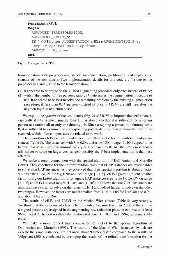
Function kRJVI;BeginADVANCED_TRANSFORMATION;AUGROWRED_6BEST_s;If f ≤ 0.1k then AUGMENTATION_s Else AUGMENTATION_P_s;Compute optimal value Optimum;LAPJVI := Optimum

End.

Fig. 3 The algorithm kRJVI

transformation with preprocessing, β-best implementation, partitioning, and exploits thesparsity of the cost matrix. Two implementation details for this code are (1) due to thepreprocessing and (2) due to the transformation;

(1) it appeared to be best to do the k−best augmenting procedure only once instead of twice;(2) with f the number of free persons, ratio f/k determines the augmentation procedure to

use. It appeared to be best to solve the remaining problem by the existing augmentationprocedure, if less than 0.1k persons (instead of 0.8n in kRJV) are still free after theaugmenting row reduction phase.

We exploit the sparsity of the cost matrix (Fig. 2) of kRJVI to improve the performance,especially if k/n is much smaller than 1. It is stored whether it is sufficient for a certainperson to examine all or only one dummy job. Since assigning a person to a dummy costs0, it is sufficient to examine the corresponding potentials v. So, fewer elements have to bescanned, which often compensates the related extra work.

The algorithm kRJVI is often 2–4 times faster than kRJV for the uniform random in-stances (Table 3). The instances with k = 0.8n, and n1 = 1500, range [1,103] appear to beharder, maybe as more row minima are equal. Compared to RLAP, the problem is gener-ally harder to solve on larger cost ranges; possibly the β-best implementation is then lesseffective.

We make a rough comparison with the special algorithm of Dell’Amico and Martello(1997). They concluded for the uniform random class that kLAP instances are much harderto solve than LAP instances, as they observed that their special algorithm is about a factor5 slower than LAPJV for k ≥ 0.9n and cost range [1,105]. kRJVI gives a (much) smallerfactor: using our fastest algorithms for square LAP instances (see Table 1), LAPJV on range[1,103] and RJVI on cost ranges [1,102] and [1,105], it follows that the kLAP instances arealmost always easier to solve on the range [1,102] and indeed harder to solve on the othertwo ranges. However, the factors are much smaller, from 1.15 to 1.65 for k = 0.8n and 0.9n;and about 1 for k = 0.99n.

The results of kRJV and kRJVI on the Machol-Wien classes (Table 4) vary strongly.We think that the randomized class is hard to solve, because less than 2.5% of the k to beassigned persons are assigned in the augmenting row reduction phase in contrast to at least96% in RLAP. The best results of the randomized class (k = 0.2n and 0.99n) are remarkablyclose.

We make a more refined time comparison of kRJVI to the special algorithm ofDell’Amico and Martello (1997). The results of the Machol-Wien instances (which areexactly the same instances) are obtained about 9 times faster compared to the results ofVolgenant (2004), confirmed by averaging the results of the refined transformation for the

452 Ann Oper Res (2010) 181: 443–462

Table 3 The results for the random k-LAP instances; kRJV and kRJVI times in ms

k n1 & n2 Range [1,102] Range [1,103] Range [1,105]kRJV kRJVI φ in % kRJV kRJVI φ in % kRJV kRJVI φ in %

0.2n1 500 22 2 90.9 22 6 72.7 21 7 66.7

1000 75 21 72.0 85 28 67.1 87 23 73.6

1500 169 46 72.8 195 55 71.8 205 60 70.7

0.4n1 500 20 7 65.0 25 13 48.0 26 12 53.8

1000 72 29 59.7 88 38 56.8 133 52 60.9

1500 156 69 55.8 402 249 38.1 404 127 68.6

0.6n1 500 25 10 60.0 31 19 38.7 35 23 34.3

1000 73 40 45.2 259 151 41.7 250 127 49.2

1500 162 105 35.2 316 153 51.6 828 332 59.9

0.8n1 500 43 19 55.8 34 26 23.5 47 36 23.4

1000 102 54 47.1 238 164 31.1 333 263 21.0

1500 172 123 28.5 727 508 30.1 1047 804 23.2

0.9n1 500 32 22 31.3 33 25 24.2 44 38 13.6

1000 185 62 66.5 183 169 7.7 301 296 1.7

1500 271 139 48.7 522 376 28.0 930 864 7.1

0.99n1 500 25 26 4.0 36 33 8.3 41 34 17.1

1000 128 102 20.3 159 145 8.8 260 236 9.2

1500 257 171 33.5 389 353 9.3 699 656 6.2

Average 49.1 36.5 36.7

Table 4 The entrances are ratios of times of kRJVI and the algorithm of Dell’Amico and Martello (1997); aratio >1 indicates that kRJVI is faster

n1 & n2 k Uniform class Machol Wien

[1,102] [1,103] [1,105] Randomized Standard

500 0.2n1 4.00 1.17 3.14 0.48 0.19

0.4n1 1.14 2.31 3.00 0.55 0.35

0.6n1 0.80 2.16 2.48 0.65 0.77

0.8n1 2.11 2.68 3.19 1.88 1.43

0.9n1 1.95 3.60 3.86 2.17 1.99

0.99n1 2.00 3.90 6.14 1.63 2.77

uniform class with n = 500. In Volgenant (2004) the results have been obtained on an AMDK6 333 MHz processor, indicating a ratio of about 3 to the personal computer used in ourresearch; Volgenant (2004) assumed that these results are obtained about a factor 18 fasterthan the special algorithm. We think that the additional speed up is due to the programminglanguage (Delphi 6 versus Turbo Pascal) and to the allocations of the data structures (staticversus more dynamic pointers).

Thus, to fairly although roughly compare the solution times of the algorithms to eachother we divided all computing times of the special algorithm by a factor of 162 (= 9 × 18)and rounded them to integers.

Ann Oper Res (2010) 181: 443–462 453

Table 5 The results for the Machol-Wien k-LAP instances; kRJV and kRJVI times in ms

k n1 & n2 Randomized Standard

kRJV kRJVI φ in % kRJV kRJVI φ in %

0.2n1 500 179 58 67.6 550 246 55.3

1000 1458 404 72.3 4219 1331 68.5

1500 4722 1098 76.7 14039 3715 73.5

0.4n1 500 382 100 73.8 970 490 49.5

1000 2792 846 69.7 7590 2963 61.0

1500 9469 2752 70.9 25131 8531 66.1

0.6n1 500 414 129 68.8 1275 682 46.5

1000 3460 1140 67.1 9751 4564 53.2

1500 11677 3553 69.6 32688 13555 58.5

0.8n1 500 265 108 59.2 1361 837 38.5

1000 2789 1050 62.4 10694 5717 46.5

1500 9533 3255 65.9 35578 17416 51.0

0.9n1 500 205 93 54.6 1277 852 33.3

1000 1966 740 62.4 10440 6020 42.3

1500 6493 2631 59.5 35087 18540 47.2

0.99n1 500 104 96 7.7 1189 850 28.5

1000 745 571 23.4 10059 6076 39.6

1500 1845 1237 33.0 33445 18782 43.8

Average 59.1 50.2

Table 5 shows this comparison between the special algorithms and kRJVI for n = 500.On these problem instances, kRJVI is much faster for almost all uniform random instances.The rather large ratio of k = 0.2n and the range [1,102] may be due to the small computationtimes, making them less precise. For the Machol-Wien instances the special algorithm isfaster if k ≤ 0.6n and kRJVI is faster if k > 0.6n. We finally note that kRJVI is easier toimplement than the special algorithm.

4 The LAP with outsourcing

To allow for the alternative of sourcing or contracting out internal jobs to external machines(or persons) and processing external jobs on internal machines, Wiel Vander and Sahinidis(1997) considered the assignment problem with external interactions (APEX). They formu-lated it as a LAP with a single unrestricted variable and developed a special primal-dualalgorithm. The mathematical model maintains the problem’s special structure and its size:

(APEX) Minimize∑

(i,j)∈A cij xij

subject to∑

j∈N2(i) xij = 1, i ∈ N1∑

i∈N1(j) xij = 1, j ∈ N2

xij ≥ 0, (i, j) ∈ A\(i◦, j ◦)

xi◦j◦ ∈ Z

454 Ann Oper Res (2010) 181: 443–462

Fig. 4 The cost matrix of theLAPout transformation

where i◦ represents all external persons to which jobs can be assigned to and j ◦ representsall external jobs to which persons can be assigned to. Each internal person can either beassigned to an available internal job or outsourced to an external job. Similarly, each internaljob can either be assigned to an available internal person or outsourced to an external person.We assume that |N1(j

◦)| = |N2(i◦)| = n1 − 1. Hence, in any feasible solution of APEX,

arc (i◦, j ◦) has a flow from j ◦ to i◦ that is one less than the number of persons (or jobs)that are assigned externally. If no person is assigned externally, there is a unit flow fromi◦ to j ◦. In general the flow on arc (i◦, j ◦) is implicitly bounded by the other constraints:−(n − 2) ≤ xi◦j◦ ≤ 1.

We can solve the APEX by standard LAP algorithms, while keeping the special structureof APEX. We replace person i◦ by n1 −1 persons and job j ◦ by n2 −1 jobs, and duplicate allthe associated arcs. We refer to the resulting model as LAPout, the LAP with outsourcing.In the related cost matrix (Fig. 4) the external persons and jobs have 0 as index. An optimalsolution of LAPout is related to an optimal solution of APEX: set xi◦j◦ = xi◦j◦ − (n1 − 2).The optimal values zA of APEX and zL of LAPout are related by zA = zL − (n1 − 2)c00.

A drawback of LAPout is that it increases the problem size. To overcome this Wiel Van-der and Sahinidis (1997) reformulated APEX as the full assignment problem (FAP) that canbe solved by any standard LAP algorithm. While FAP does not increase the problem size, itruins the (special) structure of the cost matrix, especially the sparsity:

(FAP) Minimize∑

i∈N1\i◦∑

j∈N2\j◦ min{cij , ci0 − c00 + c0j }xij

subject to∑

j∈N2(i)\j◦ xij = 1, i ∈ N1\j ◦∑

i∈N1(j)\i◦ xij = 1, j ∈ N2\j ◦

xij ≥ 0, i ∈ N1\i◦, j ∈ N2\j ◦

If xij = 1 in an optimal solution of FAP, then it is also in an optimal solution of APEX ifcij = min{cij , ci0 − c00 + c0j }; otherwise this solution contains xij◦ = xi◦j◦ = xi◦j = 1. Theoptimal values zA and zF of APEX and FAP are related by zA = zF + c00.

Alternatively, we can reduce the size of the cost matrix of LAPout by transforming itinto the matrix of a problem denoted as LAPout’, while maintaining the special structureas follows: Subtract first c00 from the last n1 − 1 rows, then c0j − c00 from the first n2 − 1columns and finally ci0 from the first n1 − 1 rows. As the costs in the last n1 − 1 rows are

Ann Oper Res (2010) 181: 443–462 455

Fig. 5 The rectangular cost matrix of LAPout after transformation (LAPout’)

0 or ∞, it makes no difference to assign these external persons to an internal job or to anexternal one; thus it is sufficient to solve an RLAP on the LAPout’ matrix (Fig. 5).

The following theorem shows the similarity between APEX and LAPout’:

Theorem 1 An optimal solution of the RLAP solved on the LAPout’ matrix is also optimalfor the APEX problem and vice versa.

Proof First note the similarity between LAPout’ and FAP. If xij = 1 in an optimal solutionof LAPout’ then cij ≤ 0; otherwise xij◦ = 1, as that improves the criterion value. Clearly,the opposite, if xij◦ = 1 then cij > 0 also holds.

Thus, if xij = 1 in an optimal solution of LAPout’, then cij ≤ ci0 − c00 + c0j ; so it is alsoin an optimal solution of APEX, like in FAP. If on the other hand xij◦ = 1 in an optimalsolution of LAPout’, then for any unassigned internal job j, cij > ci0 − c00 + c0j ; otherwiseoutsourcing person i would not be optimal. Thus, xij◦ = xi◦j◦ = xi◦j = 1 in an optimalsolution of APEX.

The optimal value zF of FAP and zL′ of LAPout’ are related: zF follows by adding upzL′ and ci0 − c00 + c0j ∀(i, j) ∈ X, with X an optimal solution of FAP; so

zA = zL′ + c00 − (n1 − 1)c00 +∑

i∈N1\i◦ci0 +

∑

j∈N2\j◦c0j

= zL′ +∑

i∈N1\i◦ci0 +

∑

j∈N2\j◦c0j − (n1 − 2)c00.

�

The structure of the LAPout’ matrix (Fig. 5) allows less preprocessing than in the case ofk-LAP. It even appeared that preprocessing of LAPout’ gave no better computational results.

In Wiel Vander and Sahinidis (1997) the special algorithm has been compared amongothers against FAP solved by LAPJV, mainly on uniform random test instances with externalarcs c00 = 0. We focus on the influence of different values of these arcs (c00 ∈ [0, . . . ,2]R)

on the computing times, comparing the transformation LAPout’ to FAP for dense instances.Ten uniform random instances were generated and solved with different values of c00, eachrange and n = 500,750 or 1000, and cost ranges [1,R] with R ∈ [102,103,105]; the externalarcs have costs 0 and R. The times (ms) are averages of the ten instances.

Table 6 gives the computational results. FAP is solved by LAPJV as well as by RJVI,denoted as FAP and FAPI respectively. RJVoutI is LAPout’ solved by RJVI. To reduce thenumber of elements to be scanned and the number of elements to be stored, we exploitthe structure of LAPout’. Because there is only one relevant external job for each person,a person is outsourced if the cost of the selected (cheapest) assignment is non-negative.

456 Ann Oper Res (2010) 181: 443–462

Table 6 Computing times (ms)for LAP with outsourcing,c00 = 0 or R

n Range c00 = 0 c00 = R

FAP FAPI RJVoutI FAP FAPI RJVoutI

500 [1,102] 30 27 333 95 219 65

[1,103] 25 33 531 152 329 100

[1,105] 36 28 533 207 356 80

750 [1,102] 92 76 905 341 673 217

[1,103] 89 92 1807 570 1018 360

[1,105] 105 95 1960 816 1143 311

1000 [1,102] 148 131 1637 797 1458 499

[1,103] 173 178 4215 1420 2178 869

[1,105] 215 208 4750 1875 2608 770

As in the kRJVI algorithm, the sparsity is exploited in both augmentation procedures. TheLAPout’ transformation is clearly less efficient than the FAP algorithms for instances withc00 = 0, the opposite holds for instances with c00 = R, while FAPI performs poorly on theseinstances.

In FAP we set cij = min{cij , ci0 +c0j −c00}, so for large c00-values the second term is of-ten dominating. FAPI starts at once with augmenting row reduction; as a result, for each rowthe first and the second row minimum often occur at the same jobs; j1 = arg minj∈N2{c0j }and j2 = arg minj∈N2\{j1}{c0j }. Therefore, reduction transfer often fails, and many personsmust be assigned in the more time-consuming augmentation phase. FAP, however, beginswith column reduction, in which the node potentials v are given values. As a result, thefirst and the second row minima less often occur at the same jobs in the augmenting rowreduction part.

After the LAPout’ transformation, cij := cij − ci0 − c0j + c00. It is likely that row minimaoccur at similar jobs in the case that c00 is small. Though, in this case reduction transfer doestake place, but only by small values. When c00 is larger, the external job can be more oftenthe row minimum, making it easier to assign the remaining persons.

The results of FAP, FAPI and RJVoutI (Fig. 6) with c00 = 0,20, . . . ,200 and cost range[1,102] show that FAPI is the fastest code if c00 ≤ 0.65R, and RJVoutI otherwise. Similarresults can be shown with other values of n and other cost ranges. We can conclude that thetwo algorithms complement each other.

5 The (k-)LAP for replacement

Suppose the manager of a plant has the funds to replace k among the n2 machines, by newerones. He wants to optimally assign tasks to machines under maximal production or equiv-alent, minimal production cost. Caseau and Laburthe (2000) denoted this problem as thereplacing k machines linear assignment problem (k-LAPrep), given that new machines aremore efficient than older ones. They assume to replace exactly k machines, even if this givesworse results. We formulate the more general case omitting the latter restriction and whereold machines may be more or less efficient than new ones. We develop a transformation thatenables to solve it as a RLAP.

Let the (production) cost of processing task i be cij on machine j and dij on a replacedmachine j . Assume without loss of generality 1 ≤ k ≤ n1 ≤ n2 and positive costs. Define

Ann Oper Res (2010) 181: 443–462 457

Fig. 6 Results for LAP with outsourcing, n = 750, and 0 ≤ c00 ≤ 200

m2 = n2 and add m2 machines to N2 at cost dij ; thus we have n2 = 2m2 and ci,m2+j = dij ,i ∈ N1, j ∈ N2 and we can formulate k-LAPrep as an RLAP with one extra constraint:

n1∑

i=1

n2∑

j=m2+1

xij ≤ k

We transform k-LAPrep into an RLAP denoted as k−LAPrep’, defining m1 = n1 and weadd m2 − k dummy nodes to N1, at cost:

cij ={

0, for i = m1 + 1, . . . , n1 and j = m2 + 1, . . . , n2,∞, otherwise,

with n1 = m1 + m2 − k. Theorem 2 is proven similarly as the simple k-LAP transformationin Volgenant (2004).

Theorem 2 The problems k-LAPrep’ and k-LAPrep are equivalent.

Proof A solution of k-LAPrep can be extended to a solution of k-LAPrep’ with the samecriterion value, by adding m2 − k (zero cost) slack assignments. There are many equivalentsolutions for k-LAPrep’, thus many solutions of k-LAPrep’ correspond to one solution ofk-LAPrep, to be found by deleting the slack assignments of the k-LAP’ solution.

Let S∗ be an optimal solution of k-LAPrep with criterion value z(S∗) = z∗; as shown,it can be extended to a feasible solution Se of k-LAPrep’, with the same criterion valuez′(Se) = z∗. Clearly Se is also an optimal solution of k-LAPrep’.

Suppose S ′ is an optimal solution of k-LAPrep’ with criterion value z′(S ′) = z′. ThenS ′ contains m2 − k slack assignments of 0 cost, because all non-slack c-values are positive.Therefore, S ′ contains at most k, say h (h ≤ k), non-slack assignments to new machines(i.e., i = 1, . . . ,m1 and j = m2 + 1, . . . , n2) and at least m1 − h non-slack assignments toold machines (i.e., i = 1, . . . ,m1 and j = 1, . . . , n1). Deleting the slack assignments of S ′forms a feasible solution, say S ′′, for k-LAPrep and z(S ′′) = z(S ′). Now z′(S ′) > z∗ = z′(Se)

contradicts the optimality of S ′, i.e., z′(S ′) = z′(Se). Thus S ′′ is an optimal solution of k-LAPrep; i.e., z(S ′′) = z(S∗) and the problems k-LAPrep’ and k-LAPrep are equivalent. �

458 Ann Oper Res (2010) 181: 443–462

Fig. 7 The cost matrix of k-LAPrep after transformation (k-LAPrep’)

It is efficient, see Volgenant (2004), to avoid degeneracy in the set of feasible solutionsof a problem, by replacing the zero elements of k-LAPrep’ by ∞ in the rows

i = m1 + 1, . . . , n1 and j = m2 + 1, . . . , n2 − k and j �= i + m2 − m1

resulting in the matrix of Fig. 7.This cost matrix does not necessarily include or exclude any assignments. Yet, it is

easy to apply preprocessing, as we can assign all dummy tasks i (i = m1 + 1, . . . , n1)

to the first m2 − k new machines j , at 0 cost, i.e., assign dummy task i to machinej = m2 + i − m1 and solve the remaining problem by an adapted RJV algorithm (denotedas RLAPrepI).

Exploiting efficiently the sparsity of the cost matrix instead of actually transforming thatmatrix, it is sufficient to check whether the chosen task is a real or a dummy one. For eachdummy, say d , one only has to scan the node potentials of the jobs

j ∈ {j | j = d + m2 − m1 or j = n − k + 1, . . . , n}.

Table 7 gives computational results on the realistic case that new machines produce cheaperthan old ones, although the production costs on new and old machines can be arbitrary. Wegenerated uniform random production costs with cij for processing task i on old machinej (i = 1, . . . , n1, j = 1, . . . ,m2) and with costs in range [1, cij ] for processing task i on anew (replaced) machine j (i ∈ N1, j ∈ N2). We generated 10 instances for each value ofn1 = n2 = n and cost ranges [1,R], R ∈ {102,103,106}, with the number of new as well asold machines n ∈ {500,750,1000} and k ∈ {0.01,0.1,0.25,0.50,0.75,0.90,0.99}n.

Caseau and Laburthe (2000) gave computational results only for instances up to size40, as the logic constraint approach fails for larger sizes. Since we know of no other (spe-cial) code for k-LAPrep we demonstrate the effect of the improvements by comparing 2codes. The code denoted by kRJVrep transforms k-LAPrep to kLAPrep’ and solves theremaining problem with RJV. In the transformed matrix n = 2m2, the numbers of ma-chines and of tasks have chosen to be equal in the considered problem instances, i.e.,m2 = m1.

Although the new machines produce tasks cheaper than the old ones (cij > dij ), it isnot always best to replace all the k machines. It appears that up to k = 0.75n almost all

Ann Oper Res (2010) 181: 443–462 459

Table 7 Computing times (in ms) for kLrep(I) with more efficient new machines (L short for LAP)

k n Range [1,102] Range [1,103] Range [1,106]kLrep kLrepI φ in % kLrep kLrepI φ in % kLrep kLrepI φ in %

0.01n 500 180 84 53.3 352 173 50.9 682 394 42.2

750 532 197 63.0 863 399 53.8 2006 1228 38.8

1000 855 217 74.6 1655 678 59.0 4489 2503 44.2

0.1n 500 375 61 83.7 599 227 62.1 1460 876 40.0

750 1131 95 91.6 1949 588 69.8 4931 2927 40.6

1000 2513 164 93.5 4426 999 77.4 11806 7131 39.6

0.25n 500 446 61 86.3 726 289 60.2 1570 1047 33.3

750 1517 128 91.6 2435 713 70.7 5329 3591 32.6

1000 3662 223 93.9 5617 1221 78.3 12366 8408 32.0

0.5n 500 211 30 85.8 509 214 58.0 983 754 23.3

750 772 69 91.1 1570 395 74.8 3290 2475 24.8

1000 2003 104 94.8 3197 379 88.1 7628 5788 24.1

0.75n 500 23 14 39.1 97 47 51.5 226 159 29.6

750 125 89 28.8 215 102 52.6 781 568 27.3

1000 360 145 59.7 331 174 47.4 1794 1290 28.1

0.9n 500 17 12 29.4 22 18 18.2 20 9 55.0

750 41 32 22.0 46 37 19.6 50 30 40.0

1000 106 110 −3.8 79 61 22.8 90 50 44.4

0.99n 500 11 13 −18.2 18 16 11.1 18 11 38.9

750 35 30 14.3 37 33 10.8 40 23 42.5

1000 90 85 5.6 65 52 20.0 74 43 41.9

Average 56.2 50.3 36.4

the k machines are actually replaced and that for higher values of k the replacement per-centage drops to a minimum of 72%. The average improvement factor φ of kRJVrepIis 47.6 % and the results are less sensitive to hard instances, i.e., φ is larger than aver-age for most of the hardest instances. Averaging over the times, kRJVrepI is more than3 times faster than kRJVrep. Instances with k = 0.25n are on average the hardest tosolve.

6 Summary and conclusions

We considered the rectangular LAP, i. e., the number of persons differs from the numberof jobs and improved an existing algorithm to solve it more efficiently, resulting in thealgorithm RJVI. As RJVI can detect hard problem instances during the execution of thealgorithm, it can solve such instances faster by partitioning the job set in assigned and infree jobs. The algorithm RJVI also uses a β-best implementation, which appears to increaserobustness over various cost ranges. It is able to efficiently solve both rectangular and squareLAP instances.

We have described and implemented preprocessing by exploiting the structure of the costmatrices to further improve the performance of RJVI on the transformation applications

460 Ann Oper Res (2010) 181: 443–462

kLAP, LAPout and kLAPrep. The special structures of the cost matrices allow additionalimprovements, which enable to solve these applications efficiently, using general and easyto implement codes. The computational results showed that one can efficiently solve thethree considered variants of the LAP by applying suited transformations and that our codesare often even much faster than existing special algorithms.

We conclude that solving the considered LAP variants by means of transformations to aRLAP appears to be flexible and efficient.

Acknowledgements We thank the Editor-in-Chief Professor Boros for useful remarks and we are gratefulto an anonymous reviewer who suggested changes that have improved the paper.

Open Access This article is distributed under the terms of the Creative Commons Attribution Noncommer-cial License which permits any noncommercial use, distribution, and reproduction in any medium, providedthe original author(s) and source are credited.

Appendix A: The augmentation part with N2(i) partitioned into P(i) and Q(i)

Procedure AUGMENTATION_P;Beginfor all free i∗ doBeginINITIALIZE;repeatif SCAN={} thenBeginSELECT_OBJECTS;if d[j ] <= μ; then goto augment

End;select any j∗ ∈ SCAN; i := y[j∗];SCAN:=SCAN-{j∗}; READY:=READY+{j∗};u1 := c[i, j∗] − v[j∗] − μ;EXAMINE_Q;if h = μ then goto augment;EXAMINE_P;

until false; (*repeat ends with go to augment*)End;

augment:for all k ∈ READY do v[k] := v[k] + d[k] − μ; (*price updating*)repeat (*augmentation*)

i :=pred[j ];y[j ] := i;k := j ; j := x[i];x[i] := k;until i = i∗;

EndEnd;

Procedure INITIALIZE;Beginbuildheap(Q[i∗]); j := Q[i∗,1]; pred[j ] := i∗;d[j ] := c[i∗, j ];READY:={}; SCAN:={}; TODOa:= {all assigned columns}; TODOu:={j};UNLAB:={all unassigned columns}-{j};for all j ∈TODOa do Begin d[j ] := c[i∗, j ] − v[j ]; pred[j ] := i∗ End

End;

Comment all possible job sets during the augmentation phase are mutually disjoint andREADY ∪ SCAN ∪ TODOa ∪ TODOb ∪ UNLAB = N;

Ann Oper Res (2010) 181: 443–462 461

Procedure SELECT_OBJECTS;Begin

μ := min{d[j ]|j ∈TODOa}; SCAN:={j |d[j ] = μ}; TODOa:=TODOa-SCAN;j := min{d[k]|k ∈TODOu};

End;

Procedure EXAMINE_Q;Beginif Q[i] = {} then buildheap(Q[i])else if Q[i,1] is assigned thenrepeat delete(Q[i,1]) until Q[i,1] is free;

j := Q[i,1];h := c[i, j ] − u1;if h = μ then pred[j ] :=ielse if j ∈UNLAB thenBegin d[j ] := h; pred[j ] := i; TODOu:=TODOu+{j}; UNLAB:=UNLAB-{j} End

else if h < d[j ] then Begin h := d[j ]; pred[j ] := i EndEnd;

Procedure EXAMINE_P;Beginfor all j ∈TODOa do if c[i, j ] − v[j ] − u1 < d[j ] thenBegin

d[j ] := c[i, j ] − v[j ] − u1; pred[j ] := i;if d[j ] = μ then Begin SCAN:=SCAN+{j}; TODO:=TODO-{j} End

EndEnd.

Appendix B: The augmenting row reduction part with the k-best implementation

Procedure AUGROWRED_kBEST;BeginFREE:={all free persons}; b[i] := {};H [i] := {};for all i ∈FREE dorepeatif b[i] �= {} thenBegin

j := 0;for all k ∈ H [i] doif c[i, k] − v[k] ≤ b[i] then j := j + 1;

if j < 2 then recompute H [i] and b[i];End

else compute H [i] and b[i];u1 := min{c[i, j ] − v[j ]|j ∈ H [i]};select j1 with c[i, j1] − v[j1] = u1;u2 := min{c[i, j ] − v[j ]|j ∈ H [i], j <> j1};select j2 with c[i, j2] − v[j2] = u2;if u1 < u2 then v[j1] := v[j1] − (u2 − u1)

else if j1 is assigned then j1 := j2k := y[j1]; if k > 0 then x[k] := 0;x[i] := j1;y[j1] := i; i := k;

until u1 = u2 (*no reduction transfer*) or k = 0 (*augmentation*)End.

References

Bertsekas, D. P., & Castañon, D. A. (1992). A forward reverse auction algorithm for asymmetric assignmentproblems. Computational Optimization and Applications, 1, 277–297.

462 Ann Oper Res (2010) 181: 443–462

Bertsekas, D. P., Castañon, D. A., & Tsaknakis, H. (1993). Reverse auction and the solution of asymmetricassignment problems. SIAM Journal on Optimization, 3, 268–299.

Burkard, R., Dell’Amico, M., & Martello, S. (2009). Assignment Problems. Philadelphia: Society for Indus-trial and Applied Mathematics.

Caseau, Y., & Laburthe, F. (2000). Solving weighted matching problems with constraints. Constraints, anInternational Journal, 5, 141–160.

Dell’Amico, M., & Martello, S. (1997). The k-cardinality assignment problem. Discrete Applied Mathemat-ics, 76, 103–121.

Dell’Amico, M., & Toth, P. (2000). Algorithms and codes for dense assignment problems: the state of the art.Discrete Applied Mathematics, 100, 17–48.

Goldberg, A. V., & Kennnedy, J. R. (1995). An efficient cost scaling algorithm for the assignment problem.Mathematical Programming, 71, 153–177.

Hsieh, A. J., Fan, K. C., & Fan, T. I. (1995). Bipartite weighted matching for on-line handwritten Chinesecharacter recognition. Pattern Recognition, 28, 143–151.

Jonker, R., & Volgenant, A. (1987). A shortest augmenting path algorithm for dense and sparse linear assign-ment problems. Computing, 38, 325–340.

Knuth, D. E. (1981). The Art of Computer Programming, Vol. 2: Seminumerical Algorithms. Reading:Addison-Wesley.

Machol, R. E., & Wien, M. (1976). A hard assignment problem. Operations Research, 24, 190–192.Mosheiov, G., & Yovel, U. (2006). Minimizing weighted earliness-tardiness and due-date cost with unit

processing-time jobs. European Journal of Operational Research, 172, 528–544.Pinedo, M. (2002). Scheduling Theory, Algorithms, and Systems (2nd edn.). Upper Saddle River: Prentice

Hall.Wiel Vander, R. J., & Sahinidis, N. V. (1997). The assignment problem with external interactions. Networks,

30, 171–185.Volgenant, A. (1996). Linear and semi-assignment problems, a core oriented approach. Computers & Oper-

ations Research, 10, 917–932.Volgenant, A. (2004). Solving the k-cardinality assignment problem by transformation. European Journal of

Operational Research, 157, 322–331.