
Solutions to Decomposed Branching Trajectories with Powered ...
162
Solutions to Decomposed Branching Trajectories with Powered Flyback Using Multidisciplinary Design Optimization A Thesis Presented to The Academic Faculty by Laura Anne Ledsinger In Partial Fulfillment of the Requirements for the Degree of Doctor of Philosophy in Aerospace Engineering Georgia Institute of Technology July 2000
Transcript of Solutions to Decomposed Branching Trajectories with Powered ...

Solutions to Decomposed Branching Trajectories with
Powered Flyback Using Multidisciplinary Design
Optimization
A Thesis
Presented to
The Academic Faculty
by
Laura Anne Ledsinger
In Partial Fulfillmentof the Requirements for the Degree of
Doctor of Philosophy in Aerospace Engineering
Georgia Institute of Technology
July 2000

Solutions to Decomposed Branching Trajectories with
Powered Flyback Using Multidisciplinary Design
Optimization
Approved:
__________________________________________John R. Olds, Chairman
__________________________________________R. Braun
__________________________________________D. Mavris
Date Approved by Chairman __________________

To all the teachers throughout my life, my family foremost among them

iv
ACKNOWLEDGEMENTS
There are many people whom I would like to thank. All those who have touched my
life in any positive way deserve some recognition. All those who have helped me with my
education and especially with my doctoral pursuits deserve recognition and my deepest
appreciation. A good number of those people are listed below.
My advisor, Dr. John R. Olds, is one of the most intelligent people I have ever had
the privilege to know and work with. Thank you, Dr. Olds, for imparting a small amount of
your knowledge to me. Thank you for your comments, suggestions, edits, and advice
concerning this thesis and all my other work. I have truly appreciated your giving me the
opportunity to be the ‘guinea pig.’
Thank you to Dr. Bobby Braun and Dr. Dimitri Mavris, the other members of my
thesis advisory committee. I realize that both of you are extremely busy men and I have
appreciated your time. I have also appreciated your comments and suggestions, which have
been invaluable.
Dr. Lakshmi Sankar and Dr. Daniel Schrage, of my thesis reading committee, thank
you both for your time and ideas.
There are more people that I am indebted to for helping me complete my work at
Georgia Tech. Dr. Jeff Jagoda, you have my sincerest gratitude for your continued support
– for aiding me in becoming Dr. Olds’ student, for helping Hitoshi, Lee, and I through a
difficult time, and for finding me some needed funding. While I’m on the subject of
funding, I would like to express my appreciation to the Georgia Space Grant Consortium
and the NASA Marshall Space Flight Center for their sponsoring my research. I thank Mr.
D. R. Komar of NASA Marshall and Mr. Dick Kohrs of Kistler Aerospace whose help
with the applications of this research, Stargazer and the Kistler K-1, respectively, enabled
me to complete this thesis. I would also like to thank Mr. John Riehl of the NASA Glenn
Research Center for his elucidation on OTIS options.
I owe a great amount of thanks to the people whom I’ve worked with every day in
the Space Systems Design Lab. Irene Budianto, thank you for keeping me sane and for

v
helping to give me hope and perseverance. You are the best cubemate and a generous and
true friend. Thanks also to John Bradford, Dave McCormick, Dave Way, Jeff Scott, Jeff
Whitfield, Ashraf Charania, Kris Cowart, Kirk Sorensen, Brad St. Germain, and Jeff
Tooley; your help in class, in the lab, and at other times has been appreciated. To all my
friends and lab mates, thank you for your assistance with my research and for being my
friends, and good luck to you in your future endeavors.
Some other friends and coworkers from Aerospace Engineering that I would like to
thank are: Anurag Gupta, Taih-Shyun Lee, Hitoshi Morimoto, Alex Leonessa, Pete
Thomas, Kelsey Watts, Catherine Matos, and Sammy Holland. I appreciate everything you
all have done for me on both professional and personal levels.
To my friend, Tisha Meeker, thanks for having faith in me. To my friends and
former college roommates: Kelly Collins and Milly Kali, your support has been
immeasurable and your friendship priceless. Thank you to all three of you for being there
when I’ve needed you.
With great gratitude, I would like to recognize my family and the Krothapalli family.
Your words of encouragement and acts of kindness have been of immense help through the
years.
A special thank you to my sister, Barbara Ledsinger. You are my dearest friend and
an inspiration. Thank you for your help, love, and encouraging presence over the years.
Words like thanks, appreciation, and gratitude are certainly not enough to express
what I owe my parents, Bob and Martha Ledsinger, for their years of sacrifice, patience, and
love. I will always be grateful, Mom and Dad, for the love of learning that you have instilled
in me, without which I would not have come this far. My thanks and love to you both
always.
With this last paragraph, I would like to thank the man who is first in my heart,
Krish Krothapalli. It has been a long and difficult journey to reach this point in my career
and you have made it much easier. When I wanted to quit and give up, you were always
there to give me your support, encouragement, strength, and love. I could not have
completed the journey without the generosity that you have shown, but most importantly,
not without you. Thank you, so very much.

vi
TABLE OF CONTENTS
A C K N O W L E D G E M E N T S . . . . . . . . . . . . . . . . . . . . . . . . . . . . . . . . . . . . . . . . . . . . . . . . . . . . . . . . . . . . . . . . . . . . . . . . . . i v
LIST OF TABLES . . . . . . . . . . . . . . . . . . . . . . . . . . . . . . . . . . . . . . . . . . . . . . . . . . . . . . . . . . . . . . . . . . . . . . . . . . . . . . . . . . . x
L I S T O F F I G U R E S . . . . . . . . . . . . . . . . . . . . . . . . . . . . . . . . . . . . . . . . . . . . . . . . . . . . . . . . . . . . . . . . . . . . . . . . . . . . . . . . . x i
N O M E N C L A T U R E . . . . . . . . . . . . . . . . . . . . . . . . . . . . . . . . . . . . . . . . . . . . . . . . . . . . . . . . . . . . . . . . . . . . . . . . . . . . . . . . x i i i
SUMMARY . . . . . . . . . . . . . . . . . . . . . . . . . . . . . . . . . . . . . . . . . . . . . . . . . . . . . . . . . . . . . . . . . . . . . . . . . . . . . . . . . . . . . . . x v i i
CHAPTER I: INTRODUCTION . . . . . . . . . . . . . . . . . . . . . . . . . . . . . . . . . . . . . . . . . . . . . . . . . . . . . . . . . . . . . . . . . . 1
1.1 THE DEFINITION OF BRANCHING TRAJECTORIES....................................................................1
1.2 MOTIVATION FOR RESEARCH ............................................................................................3
1.3 RESEARCH GOALS ...........................................................................................................5
1.4 RESEARCH OBJECTIVES ....................................................................................................5
1.5 APPROACH.....................................................................................................................6
1.6 ORGANIZATION OF THE THESIS ..........................................................................................7
CHAPTER II: TRAJECTORY OPTIMIZATION: AN OVERVIEW... . . . . . . . . . . . . . . . . . . . . .9
2.1 TRAJECTORY OPTIMIZATION IN GENERAL ............................................................................9
2.2 A GENERAL VEHICLE IN FLIGHT......................................................................................10
2.3 SOLUTION SCHEMES FOR TRAJECTORY OPTIMIZATION .........................................................11
2.3.1 Optimal Control....................................................................................................11
2.3.2 Direct Numerical Methods........................................................................................12
2.4 TRAJECTORY OPTIMIZATION PROGRAMS: OTIS AND POST.................................................12
2.5 THE OPTIMIZATION OF BRANCHING TRAJECTORIES..............................................................14
2.5.1 Branching Trajectory Optimization for this Research.....................................................15
2.5.2 The ‘One-and-Done’ and Manual Iteration Methods.......................................................16
2.5.3 Branching Trajectory Optimization in the Launch Vehicle Community.............................19
2.5.4 Summary..............................................................................................................20
vii
CHAPTER III: A BRIEF SYNOPSIS OF MULTIDISCIPLINARY DESIGN
O P T I M I Z A T I O N . . . . . . . . . . . . . . . . . . . . . . . . . . . . . . . . . . . . . . . . . . . . . . . . . . . . . . . . . . . . . . . . . . . . . . . . . . . . . . . . . . . . 2 1
3.1 THE STANDARD OPTIMIZATION FORM ..............................................................................21
3.2 DESIGN AND OPTIMIZATION............................................................................................22
3.2.1 Design.................................................................................................................22
3.2.2 Optimization of Designs..........................................................................................23
3.3 MULTIDISCIPLINARY DESIGN OPTIMIZATION......................................................................24
3.4 PARAMETRIC AND STOCHASTIC METHODS .........................................................................24
3.5 DECOMPOSITION METHODS.............................................................................................26
CHAPTER IV: MDO DECOMPOSITION METHODS IN DETAIL.. . . . . . . . . . . . . . . . . . . . . .28
4.1 FIXED-POINT ITERATION................................................................................................28
4.2 OPTIMIZATION-BASED DECOMPOSITION ............................................................................29
4.3 COLLABORATIVE OPTIMIZATION .....................................................................................32
4.4 POST-OPTIMALITY CONDITIONS FOR COLLABORATIVE OPTIMIZATION ....................................35
4.5 SUMMARY OF DECOMPOSITION METHODS..........................................................................37
CHAPTER V: THE BRANCHING TRAJECTORY PROBLEM FORMULATED USING
M D O . . . . . . . . . . . . . . . . . . . . . . . . . . . . . . . . . . . . . . . . . . . . . . . . . . . . . . . . . . . . . . . . . . . . . . . . . . . . . . . . . . . . . . . . . . . . . . . . . . 3 9
5.1 THE FIXED-POINT ITERATION METHOD ............................................................................40
5.2 THE OPTIMIZATION-BASED DECOMPOSITION METHODS........................................................41
5.3 THE COLLABORATIVE OPTIMIZATION METHOD ..................................................................42
CHAPTER VI: THE FIRST APPLICATION: THE KISTLER K-1 LAUNCH VEHICLE
. . . . . . . . . . . . . . . . . . . . . . . . . . . . . . . . . . . . . . . . . . . . . . . . . . . . . . . . . . . . . . . . . . . . . . . . . . . . . . . . . . . . . . . . . . . . . . . . . . . . . . . . 4 4
6.1 THE KISTLER K-1 LAUNCH VEHICLE.................................................................................44
6.2 THE KISTLER K-1 TRAJECTORY ........................................................................................46
6.3 THE OBJECTIVE FUNCTION FOR THE KISTLER K-1 ................................................................48
CHAPTER VII: RESULTS FOR THE K-1 LAUNCH VEHICLE . . . . . . . . . . . . . . . . . . . . . . . . . 4 9
7.1 METHODS WITH CONFLICTING OBJECTIVE FUNCTIONS.........................................................49
7.1.1 ‘One-and-Done’ Method...........................................................................................49
7.1.2 Manual Iteration Method Results...............................................................................51
7.2 THE SYSTEM-LEVEL OPTIMIZER.......................................................................................52
7.3 MULTIDISCIPLINARY DESIGN OPTIMIZATION RESULTS.........................................................53
viii
7.3.1 Fixed-Point Iteration Method....................................................................................54
7.3.2 Partial Optimization-Based Decomposition..................................................................58
7.3.3 Full Optimization-Based Decomposition.....................................................................61
7.3.4 Collaborative Optimization......................................................................................63
7.4 SUMMARY ...................................................................................................................68
CHAPTER VIII: STARGAZER : THE SECOND APPLICATION. . . . . . . . . . . . . . . . . . . . . . . . 74
8.1 STARGAZER ...................................................................................................................74
8.2 THE DESIGN STRUCTURE MATRIX FOR STARGAZER...............................................................76
8.3 STARGAZER’S BRANCHING TRAJECTORIES...........................................................................80
8.4 THE OBJECTIVE FUNCTION FOR STARGAZER’S BRANCHING TRAJECTORIES.................................83
CHATPER IX: RESULTS FOR STARGAZER . . . . . . . . . . . . . . . . . . . . . . . . . . . . . . . . . . . . . . . . . . . . . . 8 4
9.1 METHODS WITH CONFLICTING OBJECTIVE FUNCTIONS.........................................................84
9.1.1 ‘One-and-Done’ Method...........................................................................................84
9.1.2 Manual Iteration Method..........................................................................................87
9.2 THE SYSTEM-LEVEL OPTIMIZER.......................................................................................87
9.2.1 System-Level Constraints for Stargazer ......................................................................88
9.3 MULTIDISCIPLINARY DESIGN OPTIMIZATION RESULTS ...................................................90
9.3.1 Optimization-Based Decomposition...........................................................................91
9.3.2 Collaborative Optimization......................................................................................92
9.4 SUMMARY ...................................................................................................................97
CHATPER X: CONCLUSIONS AND RECOMMENDATIONS. . . . . . . . . . . . . . . . . . . . . . . . . . .106
10.1 CONCLUSIONS AND OBSERVATIONS ...............................................................................106
10.1.1 Conclusions.......................................................................................................107
10.1.2 The New Method for Branching Trajectory Problem Solutions.....................................111
10.1.3 Observations.......................................................................................................113
10.2 RECOMMENDATIONS FOR FUTURE RESEARCH ..................................................................117
APPENDIX A: Weight Breakdown for the Kistler K-1 . . . . . . . . . . . . . . . . . . . . . . . . . . . . . . . . . . . . 1 2 1
APPENDIX B: Engine and Aerodynamics Information for the K-1 . . . . . . . . . . . . . . . . . . . . . 1 2 2
APPENDIX C: Final Design Variables for K-1 M e t h o d s . . . . . . . . . . . . . . . . . . . . . . . . . . . . . . . . . 1 2 4
APPENDIX D: RBCC Engine Inputs to SCCREAM for Stargazer. . . . . . . . . . . . . . . . . . . . . . 1 2 6

ix
APPENDIX E: Stargazer Engine Mult ipl iers & Scal ing Equations . . . . . . . . . . . . . . . . . . . . .129
APPENDIX F: Stargazer Weight s Response Sur faces . . . . . . . . . . . . . . . . . . . . . . . . . . . . . . . . . . . . . 131
APPENDIX G: Final Design Variables for Stargazer Methods . . . . . . . . . . . . . . . . . . . . . . . . . . 1 3 3
R E F E R E N C E S . . . . . . . . . . . . . . . . . . . . . . . . . . . . . . . . . . . . . . . . . . . . . . . . . . . . . . . . . . . . . . . . . . . . . . . . . . . . . . . . . . . . . 1 3 5
VITA . . . . . . . . . . . . . . . . . . . . . . . . . . . . . . . . . . . . . . . . . . . . . . . . . . . . . . . . . . . . . . . . . . . . . . . . . . . . . . . . . . . . . . . . . . . . . . . . 1 4 4

x
LIST OF TABLES
Table 1: Modeling Options for OTIS and POST..............................................................14
Table 2: Results for Mathematical Conflicting Objective Functions Example...................18
Table 3: Proposed MDO Solution Techniques.................................................................38
Table 4: POST Controls and Constraints for the K-1 .......................................................47
Table 5: ‘One-and-Done’ and Manual Iteration Method Results (K-1)............................50
Table 6: Size of System Optimizer for Kistler K-1 Cases.................................................53
Table 7: Targets’ Relationship to POST Decks for K-1 ...................................................65
Table 8: K-1 Results Comparison (MDO)........................................................................69
Table 9: K-1 Detailed Results Comparison (MDO)..........................................................70
Table 10: Staging Vector Results for the K-1....................................................................71
Table 11: Stargazer Controls and Constraints..................................................................81
Table 12: ‘One-and-Done’ and Manual Iteration Results for Stargazer ..........................86
Table 13: Size of System Optimizer for Stargazer Cases.................................................88
Table 14: Dry and Gross Weight Comparisons................................................................89
Table 15: Targets’ Relationship to POST Decks for Stargazer........................................94
Table 16: Stargazer Results Comparison (MDO)............................................................98
Table 17: Stargazer Detailed Results Comparison (MDO)..............................................98
Table 18: Stargazer Ratios Results Comparison..............................................................99
Table 19: Stargazer Final Staging Vector Comparison....................................................100
Table 20: Set-up Time Comparisons................................................................................109
Table 21: Communication Requirements Summary.........................................................116

xi
LIST OF FIGURES
Figure 1: RTLS Branching Trajectory...............................................................................2
Figure 2: Downrange Branching Trajectory.......................................................................3
Figure 3: A Point Mass in Flight......................................................................................10
Figure 4: Example of a TSTO’s Stages with Fuel............................................................16
Figure 5: Design Structure Matrix....................................................................................23
Figure 6: Generic FPI Diagram........................................................................................29
Figure 7: Generic OBD Diagram......................................................................................30
Figure 8: Generic CO Diagram.........................................................................................32
Figure 9: FPI for Branching Trajectories..........................................................................40
Figure 10: POBD for Branching Trajectories...................................................................41
Figure 11: FOBD for Branching Trajectories...................................................................42
Figure 12: CO for Branching Trajectories........................................................................43
Figure 13: The K-1 ...........................................................................................................45
Figure 14: The K-1 Flight Profile.....................................................................................46
Figure 15: The DSM for the K-1 ......................................................................................47
Figure 16: ‘One-and-Done’ Method Flowchart...............................................................50
Figure 17: Manual Iteration Method Flowchart................................................................52
Figure 18: FPI Flowchart, K-1 ..........................................................................................56
Figure 19: Payload Weight Tracking for FPI Method......................................................57
Figure 20: Active Constraint History for the FPI Method.................................................57
Figure 21: POBD Flowchart, K-1 .....................................................................................59
Figure 22: Payload Weight Tracking for POBD Methods...............................................60
Figure 23: Active Constraint History for the POBD Methods..........................................60
Figure 24: FOBD Flowchart, K-1 .....................................................................................61
Figure 25: Payload Weight Tracking for the FOBD Method...........................................62
Figure 26: Active Constraint History for the FOBD Method............................................63
Figure 27: CO Flowchart, K-1 ..........................................................................................64

xii
Figure 28: Payload Weight Tracking for the CO Method.................................................66
Figure 29: Active Constraint History for the CO Method.................................................67
Figure 30: System-Level Coordination for Ascent Propellant...........................................67
Figure 31: System-Level Coordination for Payload Weight.............................................68
Figure 32: Altitude versus Time for the K-1......................................................................72
Figure 33: Flyback Pitch Angle versus Time for the K-1 ..................................................73
Figure 34: Velocity versus Time for the K-1 .....................................................................73
Figure 35: Stargazer Concept...........................................................................................74
Figure 36: Stargazer Mission Profile...............................................................................75
Figure 37: Stargazer DSM...............................................................................................76
Figure 38: Main Iteration Loop.........................................................................................77
Figure 39: Baseline Packaging for Stargazer ...................................................................78
Figure 40: Stargazer’s TPS Layout..................................................................................79
Figure 41: Modified DSM for Stargazer .........................................................................80
Figure 42: ‘One-and-Done’ Flowchart, Stargazer ...........................................................85
Figure 43: Manual Iteration Method Flowchart, Stargazer ...............................................86
Figure 44: POBD Flowchart, Stargazer ...........................................................................90
Figure 45: Active Constraint and Dry Weight History for Stargazer POBD...................91
Figure 46: Dry Weight Oscillations for System-Level Iteration 12 – 16...........................92
Figure 47: CO Flowchart, Stargazer.................................................................................93
Figure 48: Dry Weight History for Stargazer CO...........................................................95
Figure 49: Active Constraint History for Stargazer CO...................................................96
Figure 50: System-Level Coordination for Altitude..........................................................96
Figure 51: System-Level Coordination for Initial Flyback Weight...................................97
Figure 52: Pitch Angles versus Time for Stargazer Ascent Trajectories..........................101
Figure 53: Typical Ascent Trajectory Plots for Stargazer................................................101
Figure 54: Angle of Attack versus Time for Stargazer Flyback Trajectories...................102
Figure 55: Bank Angle versus Time for Stargazer Flyback Trajectories.........................103
Figure 56: Groundtrack Comparison for Stargazer Flyback Trajectories........................103
Figure 57: Altitude versus Time for Stargazer Flyback Trajectories................................104
Figure 58: Velocity versus Time for Stargazer Flyback Trajectories...............................105
Figure 59: Altitude versus Time for Stargazer Upper Stage Trajectories.........................105
Figure 60: Method Structure for Branching Trajectory Solutions....................................112
Figure 61: Lockheed Martin LFBB.................................................................................118

xiii
NOMENCLATURE
ABBREVIATIONS
deg degree
Dry Stargazer booster dry weight
ft feet
ft/s feet per second
lbs pounds
log logarithm
min minutes
Mix Stargazer booster mixture ratio
MRb Stargazer booster mass ratio
MRfb Stargazer flyback mass ratio
MRus Stargazer upper stage mass ratio
nmi nautical mile
psf pounds per square foot
psi pounds per square inch
RSquare residual squared
sec seconds
Sref Stargazer booster wing planform area
USSref Stargazer upper stage wing planform area
USwg Stargazer upper stage gross weight
Wg Stargazer booster gross weight
ACRONYMS
CO Collaborative Optimization
DOE Design of Experiments

xiv
DOT Design Optimization Tool
DSM Design Structure Matrix
DDT&E Design, Development, Testing, and Evaluation
FOBD Full Optimization-Based Decomposition
FPI Fixed-Point Iteration
GA Genetic Algorithm
HSCT High Speed Civil Transport
IUS Inertial Upper Stage
KSC NASA Kennedy Space Center
LFBB Liquid Flyback Booster
LOX Liquid OXygen
LRU Line Replacement Units
MDO Multidisciplinary Design Optimization
MMFD Modified Method of Feasible Directions
NAND Nested ANalysis and Design
NASA National Aeronautics and Space Administration
OBD Optimization-Based Decomposition
OTIS Optimal Trajectories by Implicit Simulation
PERL Practical Extraction and Report Language
POBD Partial Optimization-Based Decomposition
POST Program to Optimize Simulated Trajectories
RBCC Rocket-Based Combined Cycle
RLV Reusable Launch Vehicle
RSM Response Surface Methods
RTLS Return to Launch Site
SAND Simultaneous ANalysis and Design
SCCREAM Simulated Combined-Cycle Rocket Engine Analysis Module
SLP Sequential Linear Programming
SQP Sequential Quadratic Programming
SSTO Single-Stage-to-Orbit
TABI Tailorable Advance Blanket Insulation
TPS Thermal Protection System
TSTO Two-Stage-to-Orbit
TUFI Toughened Uni-Piece Fibrous Insulation

xv
UHTC Ultra-High Temperature Ceramic
SYMBOLS
$M million dollars
A, B, and C design analyses/contributing analyses/disciplines
A, B, and C output vectors (OBD & CO)
A’, B’, and C’intermediate values for compatibility constraint formulation
A , B , and C targets for error formulation
AC and BC C’s local version of target coupling variables
BA and CA A’s local version of target coupling variables
CB and AB B’s local version of target coupling variables
cl subsystem local variables
D drag
F(x) generic objective function
g gravity
gj(x) single inequality constraint
hk(x) single equality constraint
JA, JB, and JC error between A, B, and C’s, local variables & target variables
JA error between Ascent’s local variables & target variables
JO error between Orbit’s local variables & target variables
JF error between Flyback’s local variables & target variables
Isp specific impulse
l number of equality constraints
m number of inequality constraints
mg weight, mass times gravity
n number of design variables
Ps staging vector
Ps' prescribed staging vector
P s staging vector target
T thrust
V velocity
wfb flyback fuel weight

xvi
wfb' flyback fuel weight guess
w fb flyback fuel weight target
wus upper stage weight
wus' prescribed upper stage weight
w us upper stage weight target
x design variable vector
xil lower bound of xI
xiu upper bound of xI
xss subsystem design variable vector
ε angle between velocity and thrust in the vertical plane/small tolerance
γ flight path angle

xvii
SUMMARY
In the advanced launch vehicle design community, there exists considerable interest
in fully reusable, two-stage-to-orbit vehicle designs that use ‘branching trajectories’ during
their missions. For these reusable systems, the booster must fly to a predetermined landing
site after staging occurs.
The solution to this problem using an industry-standard trajectory optimization code
typically requires at least two separate computer jobs — one for the orbital branch from the
ground to orbit (in some cases, this can be broken into two computer jobs) and one for the
flyback branch from the staging point to the landing site. These jobs are tightly coupled
and their data requirements are interdependent. In addition, the objective functions for each
computer job differ and conflict.
This research produces a method to solve these distributed branching trajectory
problems with respect to an overall system-level objective while maintaining data
consistency within the problem. This method is used to solve the trajectories of two relevant
two-stage-to-orbit vehicles: the Kistler K-1 and the Stargazer launch vehicles. Both of
these vehicles require a powered flyback. Thus, optimization contingent on the feedback of
the flyback fuel is a relevant part of this study.
The solutions of the branching trajectory problems via traditional methods, termed
‘One-and-Done’ and manual iteration, are compared with those involving the
multidisciplinary design optimization techniques of fixed-point iteration, optimization-based
decomposition, and collaborative optimization. Optimization-based decomposition was
used to solve each problem; the K-1 trajectory includes a fixed-point iteration solution. The
use of collaborative optimization as an solution technique for branching trajectories is
introduced in the solution to each problem.

xviii
Results show that proposed method involving collaborative optimization and
optimization-based decomposition performed well for both the K-1 and Stargazer
branching trajectories. The use of these methods for the Kistler K-1 problem shows that an
increase in payload weight of 1.0%, on average, could be obtained. Similarly, a reduction in
Stargazer’s dry weight of approximately 0.8% was achieved through the MDO methods.
Conclusions concerning the method outline, comparisons of the method with differing
solution techniques, staging flight path angle trends, and the automation of the optimization
process are included.

1
CHAPTER I
INTRODUCTION
Fully reusable two-stage-to-orbit vehicle designs that incorporate ‘branching’
trajectories during their ascent are of current interest in the advanced launch vehicle design
community. Unlike expendable vehicle designs, the booster of a reusable system must fly
to a designated landing site after staging. Therefore, in addition to the ascent trajectory, both
the flyback, or booster return, branch and the orbital upper stage branch are of interest and
must be simultaneously optimized in order to achieve an overall system objective. Current
and notable designs in this class include the U. S. Air Force Space Operations Vehicle
designs with their ‘pop-up’ trajectories, the Kelly Astroliner, the Kistler K-1, one of the
preliminary designs for NASA’s Bantam-X and Bimese studies, and NASA’s proposed
liquid flyback booster designs (Space Shuttle solid booster upgrade).
1.1 The Definition of Branching Trajectories
In an effort to lower costs, designers of advanced two-stage-to-orbit (TSTO) launch
vehicles are beginning to consider launch systems in which the booster stage can be
recovered, serviced, and reflown. Often the reusable booster is required to land at a
predesignated recovery site either near the original launch site (RTLS-style trajectory,
Figure 1) or downrange of the staging point (Figure 2). In these cases, the entire trajectory
is composed of three parts. The ascent trajectory follows the vehicle from launch to staging.
At this point, the trajectory is assumed to split into two ‘branches.’ One is the orbital
branch beginning at staging and following the orbital upper stage all the way to orbit. The

2
second branch, or flyback branch, starts at the staging point and follows the reusable
booster to its landing site. Due to recovery distance or out-of-plane maneuvers required, the
booster is often powered for its flight to the landing site. In simulations where the booster
is jettisoned from an orbital vehicle, it may be convenient to combine the ascent trajectory
and the orbital branch to create one computer job. The same may be said about a launch
vehicle with an upper stage that is jettisoned; the ascent trajectory and the flyback branch
may be combined.
Figure 1: RTLS Branching Trajectory

3
Figure 2: Downrange Branching Trajectory
In general, both the orbital branch and the flyback branch rely upon the ascent
trajectory for their respective initial conditions. These initial conditions are vectors
composed of geographical position, altitude, velocity, flight path angle, velocity azimuth, and
staging weight. The ascent trajectory also depends on both branches. Assuming that the
booster is powered, the amount of flyback fuel required by the booster influences the gross
lift-off weight of the vehicle and thus the ascent path. The weight of the upper stage (which
is dependent upon initial staging conditions) also affects the gross lift-off weight of the
vehicle and thus the ascent path. Consequently, all the parts of the entire trajectory are
coupled or interdependent.
1.2 Motivation for Research
In the public domain or otherwise open literature, no computationally efficient
method exists for solving branching trajectories, as defined above, that include the feedback
of data. This pertains specifically to those trajectories in which separate branches are
simulated and the data from the trajectory branches that occur after staging is required by
the ascent path.

4
Faced with the lack of a suitable solution method, today’s trajectory analysts are
forced to either 1) compromise the optimality of their solutions, or 2) create large, complex
optimization problems that are difficult to solve numerically. In the former case, later
referred to as the manual iteration method, the analyst may choose to decompose the
branching trajectory into several subproblems (one for each branch) that are individually
and sequentially optimized. In most situations, this approach will undermine any natural
compromise between the branches and lead to a suboptimal overall objective. The latter case,
later referred to as the fixed-point iteration approach, generally requires the analyst to create
a large, slow computer simulation in which all independent variables and all constraints for
each branch are treated by a single optimizer. This problem is made more difficult by the
presence of the natural coupling between the ascent and the branches of the trajectory and
the resulting iteration that must occur between them. A branching trajectory solved in this
way often exhibits numerical convergence problems and does not scale well to very large
problems.
The shortcomings in the two current state-of-practice approaches above can be
significant. At current payload delivery prices of more than $3,000/lb of payload to orbit, a
suboptimal solution that loses just 0.1% of payload for a typical medium-sized booster
would result in a loss of potential revenue of more than $500,000 per flight. Alternately,
with engineering time costing as much as $100/hour, a new solution method, that might save
25% of the time it would take an engineer fill out a payload performance map with 100’s of
branching trajectory cases, might save almost $20,000. These effects are significant and
provide some of the motivation for the present research.
As was mentioned previously, the manual iteration method results will not exploit
the compromises of the branches. These compromises are revealed through the staging
vector components. Thus, another motivating factor for this research involves identifying
potential staging vector compromises for branching trajectories in general.

5
1.3 Research Goals
It is the goal of this research, and ultimately its contribution to the field of trajectory
optimization, to develop and demonstrate a new open-literature method for solving
branching trajectories in which feedback data is accurately and efficiently modeled.
It is further a goal of this research that the new method be computationally efficient
by allowing the problem to be decomposed into smaller, more numerically manageable
subproblems (one for each branch) that can be solved in a distributed fashion. The new
method must be as simple and straightforward as possible without introducing extensive
set-up complexities or set-up times. It cannot produce a series of suboptimal solutions for
each branch nor can it produce solutions that are internally inconsistent between branches.
(Internal consistency meaning that the coupling variables produced by the branches are
numerically identical to those same variables passed into the ascent and vice versa). Lastly,
the new method should be scalable and adaptable to a wide variety of large and small
branching problems having this particular coupling characteristic.
1.4 Research Objectives
In support of the aforementioned research goals, specific research objectives (or
targets) were established to measure the success of the methodology development effort.
Some of the objectives are qualitative in nature, while others represent specific quantitative
targets. These research objectives for the new method are outlined as follows:
• Demonstrate an efficient computation approach that can be distributed on several
computing processors to reduce overall solution time enough such that the solution
process would be applicable in a vehicle design framework.
• Demonstrate an improvement of 1% or greater in the objective function relative to
the suboptimal solution of the manual iteration method.
• Decrease the computing time relative to a fixed-point iteration approach by 10% or
more for a single trajectory solution.

6
• Maintain a reasonable level of method complexity and a set-up time that is no more
than 50% greater than the set-up time of a suboptimal method like the manual iteration
method.
• Guarantee internal data consistency between the individual branches at the solution.
• Demonstrate the scalability and robustness of the new method for small and large
branching trajectory problems.
• Formulate generalities of staging vector compromises for the branching trajectory
problem.
1.5 Approach
After the current solution techniques for branching trajectories and their deficiencies
was researched, a rough framework for the new solution method was established (the full
details of the new method will be disclosed in subsequent chapters). Since an objective of
this research was that the new method be computationally efficient in terms of computation
time and distribution of computing resources, the proposed method advocates the
decomposition of the individual branches of the trajectory into separate subproblems.
Subsequently, these distributed subproblems had to be coordinated into a consistent and
optimal solution.
The field of multidisciplinary design optimization (MDO) provided several
techniques that have been successfully applied to the decomposition and subsequent
coordination of the individual subproblems. Therefore, a key element of the present
research was to examine several pertinent MDO techniques to determine their applicability
to this class of branching trajectory. Based on the results of this investigation, one MDO
solution technique was recommended for use in the overall method.
Two ‘test case’ applications were formed to help guide the development of the
method and to demonstrate its utility toward reaching the research goals and objectives. The

7
first testcase, the Kistler K-1 launch vehicle, was a relatively small, coupled branching
trajectory problem. The second testcase, the Stargazer design, was a more complex
problem in which the branching trajectory analysis was tightly coupled with other
disciplines. The evaluation of all of these analyses was necessary to evaluate the branching
trajectory performance.
In addition to their implementation in the selection of the MDO technique chosen
for the proposed method, these two testcases were also used to establish the benchmark (the
manual iteration method solution) from which comparisons could be made. These
comparisons were analyzed with respect to execution times, set-up complexity, and objective
values at the solution.
While solving the branching trajectory problem, a significant amount of time was
invested in order to understand the details of each method, automate or script many of the
analyses in the optimization process, and run thousands of individual analyses needed to
generate supporting data. This data was then used to draw conclusions and evaluate any
improvements and concurrence with the stated objectives. Based on these conclusions,
recommendations for future work were made.
1.6 Organization of the Thesis
The thesis is organized in the following manner. This chapter, Chapter I, introduces
the problem of branching trajectories and the contribution of the research. Chapters II and
III review background information on trajectory optimization, both in general and for the
branching trajectory formulation, and on multidisciplinary design optimization (MDO),
respectively. Decomposition methods are the specific methods used for analysis in this
thesis. Thus, background information and prior research with respect to MDO
decomposition methods are presented in Chapter IV. In Chapter V, the general branching
trajectory problem is formulated as MDO problems. This chapter shows specific
illustrations of the branching trajectory problem when formed using the decomposition
methods of Chapter IV. The first application, the Kistler K-1 launch vehicle, is described in
Chapter VI. Specifically, the vehicle characteristics, trajectory, and objective function are
accounted for in detail. The results for the K-1 analysis are reported on in Chapter VII.

8
Results for both traditional methods and MDO methods are analyzed. Chapter VIII
introduces the second application, Stargazer, its design structure, trajectory, and objective
function. Results with respect to traditional methods and MDO methods for the Stargazer
vehicle are examined in Chapter IX. Chapter X closes the thesis with conclusions and
recommendations for future work.

9
CHAPTER II
TRAJECTORY OPTIMIZATION: AN OVERVIEW
Much research has been performed in the area of trajectory optimization [1,2,3].
This chapter presents the background of trajectory optimization with emphasis on that
which is necessary for launch vehicle missions. The additional considerations required for
branching trajectory optimization with powered flyback, along with past research in that
specific area, is discussed.
2.1 Trajectory Optimization in General
Trajectory optimization can be defined as finding the ‘best’ path from an initial
condition to some final condition based on a certain performance index [3]. This is
achieved subject to gravitational, propulsive, and aerodynamic forces. The ‘best’ path is
contingent on the performance index, or objective function, to be optimized. The objective
function can be to maximize final weight, minimize time, or maximize distance covered. The
optimization of the trajectory usually occurs in phases, such as take-off, cruise, and landing.
Typically, the phases are optimized given initial and final events, which are subject to path
constraints.

10
2.2 A General Vehicle in Flight
A vehicle in flight can be approximated by a point mass. Figure 3 shows an
illustration of a point mass subjected to forces in flight.
L
V
D
mg
Tε
γγ
y
x
Figure 3: A Point Mass in Flight
Summing about each axis, the dynamic equations for velocity, V, and flight path
angle, γ, are given in equations 1 and 2.
m ˙ V = - D - mgsin(γ) + Tcos(ε) (1)
mV ˙ γ = L + Tsin(ε) – mgcos(γ) (2)
where L is the lifting force, D is the drag force, T is the thrust, or propulsive force, and mg is
the gravitational force. These equations can be rearranged to form the general nonlinear
longitudinal equations of motion for a vehicle [4], similar equations can be formulated for
lateral motion [4]. The general equations are then used to model the flight path. When
combined with aerodynamic, propulsive, and weight models, the equations of motion can be

11
integrated through time to produce the entire trajectory. Once an initial trajectory is
obtained, optimization can occur.
2.3 Solution Schemes for Trajectory Optimization
Solution methods for trajectory optimization problems are typically identified as
either indirect methods or direct methods [5, 6]. Indirect methods use calculus of variations
techniques [7] to characterize the optimization problem as a two-point boundary-value
problem [8, 9]. At the initial time, the costate variables, or Lagrange multipliers, must be
guessed. Since these variables are just multipliers and have no physical meaning, guessing
their initial values is very difficult and may lead to problems with convergence to the
optimum. Direct methods discretize the optimization problem through events
(distinguishing initial/final conditions) and phases (that part of the trajectory occurring
between events.) The subsequent problem is solved using nonlinear programming
techniques [10, 11]. Some indirect and direct optimization methods are considered below.
2.3.1 Optimal Control
The optimal control scheme [12] is an indirect method. It has been used to solve
many trajectory optimization problems for launch vehicles [13, 14, 15, and 16]. Optimal
control uses first variation techniques to determine necessary conditions, for an optimum,
and second variation techniques to determine sufficient conditions, to find out what kind of
optimum. Optimal control requires analytical differentiation of the equations of motion,
including the models for propulsion, atmosphere, weights, etc. In fact, to determine
satisfaction of the sufficient conditions, the equations and models must be twice
differentiable. The models are usually highly complicated equations and vehicle specific.
Thus, optimal control problems are difficult to make modular. Because these problems are
posed as two-point-boundary-value problems, a priori knowledge of the initial state
variables, final costate variables, and occurrence of path constraints is an advantage.
Without this knowledge, improper initial guesses can lead to convergence difficulty.

12
2.3.2 Direct Numerical Methods
The direct schemes which use nonlinear programming include simple shooting,
multiple shooting, and transcription, or collocation. In the shooting methods, the control
history is discretized as a polynomial, with the trajectory variables a function of the
integrated equations of motion. In the collocation method, the vehicle’s flight path is
discretized, over time intervals, as a set of polynomials for both the trajectory variables and
controls. To ensure that a physically feasible to trajectory is calculated, satisfaction of the
equations of motion is enforced at discrete points throughout the trajectory.
In both cases, nonlinear programming techniques are used to find the optimal
trajectory. These methods require gradient calculations to analyze the sensitivities of the
design variables (either controls, or controls and trajectory variables) to the objective and
constraints. These gradient calculations usually require many function calls (trajectory
simulations). However, numerical optimization schemes of shooting methods and
collocation are easily coded and allow for varying models, resulting in their being popular
methods for implementation in trajectory optimization software [17, 18, 19]. As with
indirect techniques, these methods are sensitive to the weighting scheme and initial guess.
Two popular trajectory optimization codes are described in the next section. Both
use direct methods.
2.4 Trajectory Optimization Programs: OTIS and POST
OTIS [17], Optimal Trajectories by Implicit Simulation, is a trajectory simulation
program that primarily uses nonlinear programming and collocation, although shooting is
an option. OTIS was originally developed by the Boeing Company under contract to the
Air Force and is popular throughout the trajectory optimization community. OTIS can
accommodate varying models of propulsion, weights, atmospheres, and aerodynamics. As a
result of the trajectory variables being parameterized over specific time intervals, constraint
boundaries, such as a dynamic pressure boundary, are easily simulated in OTIS.

13
The Program to Optimize Simulated Trajectories — POST I [18] was developed by
Lockheed-Martin under contract to NASA and is widely used for trajectory optimization
problems in advanced vehicle design. POST is a generalized event-oriented code that
numerically integrates the equations of motion of a flight vehicle given definitions of
aerodynamic coefficients, propulsion system characteristics, atmosphere tables, and
gravitational models. Guidance algorithms used in each phase are user-defined. Numerical
optimization, specifically nonlinear programming and direct shooting, is used to satisfy
trajectory constraints and minimize a user-defined objective function by changing
independent steering and propulsion variables along the flight path. POST runs in a batch
execution mode and depends on an input file (or input deck) to define the trajectory event
structure, vehicle parameters, independent variables, constraints, and objective function.
Both the OTIS and POST codes have various limitations and approximations
associated with their trajectory models. Table 1 lists the various options offered by these
codes. POST and OTIS each offer three- and six-degree-of-freedom simulations and point
mass approximations of the vehicle being simulated.
More intricate differences occur between the table modeling options and guidance
and steering algorithms employed. Table inputs are linearly interpolated in POST. In
OTIS, tables are modeled more complexly. Table data is curve fit with the choices of a
linear fit, cubic or quintic spline fits, or, in the most recent version of the code, a chamfered
spline fit. In addition, steering in OTIS is essentially achieved open-loop and a ramp
steering option acts as guidance for the simulations. Guidance and steering options for
POST are more varied and include: vehicle body rates, aerodynamic angles, euler angles,
and pitch plane steering; open/closed loop guidance; generalized acceleration steering; and
predictor-corrector guidance.

14
Table 1: Modeling Options for OTIS and POST
Model OTIS POST
Atmospheric Model 17 model options, including
options for wind models and
user-defined models
17 model options, including 4
for winds, 3 for turbulence, and
2 for gusts and user-defined
models
Aerodynamic Model Tables for Axial & Normal
or Lift & Drag Coefficients
Tables for Axial & Normal or
Lift & Drag Coefficients
Gravity Model 2nd –4th harmonics in the
gravity potential function
Oblate and spherical planet
options
2nd –8th harmonics in the
gravity potential function
Oblate and spherical planet
options
Numerical
Integration Methods
6 options including 4th order
Runge-Kutta, variable step
methods, and implicit
integration.
7 options including 3 Runge-
Kutta methods, variable step
methods, and methods
specialized for orbit
simulations
POST and OTIS are being improved and additions are made regularly. In addition,
users have the option to write their own supplemental algorithms. The options and
approximations listed in Table 1 are only highlights of some choices that are common in
trajectory simulation models. Ultimately, the main difference occurs in the optimization
methods employed, as previously mentioned.
2.5 The Optimization of Branching Trajectories
As explained in Chapter I, there are many different TSTO mission profiles that
exhibit branching trajectories. Future RLV’s depend on this type of trajectory because the
reusability of the vehicle is furthered by it. In the previous sections, the motivation for
trajectory optimization was reviewed. Branching trajectories are no different in that they
must also be optimized.

15
Branching trajectories can be posed as non-distributed or distributed simulations.
Non-distributed problems require one simulation that can accommodate multiple vehicle
models, which would be needed after staging. The optimizer for this problem will be large,
as it contains all the design variables and constraints for the entire branching trajectory.
This has the potential to lead to long simulation times. Distributed problems simulate the
branching trajectory as two or three separate simulations. They can be decomposed at the
staging point to result in an ascent trajectory and an upper stage trajectory and/or a flyback
trajectory. Optimization can occur at the trajectory level, at an overall system-level, or at
both levels. These solutions are explained below and in Chapter V. Simulation, or CPU,
time can be saved by posing the branching trajectory in this distributed manner.
2.5.1 Branching Trajectory Optimization for this Research
In the public domain, research is lacking with respect to branching trajectories with
powered flyback. In the same domain, it is nonexistent for such trajectories solved in a
distributed manner with an overall objective and consistent data between subproblems.
For the research presented in this thesis, branching trajectories with powered
flybacks were decomposed into distributed problems. POST, described in the previous
section, is the program that was used to simulate the trajectories. POST is currently used
for launch vehicle trajectory simulation in the Space Systems Design Lab at Georgia Tech
and is the code of which the author is intimately familiar. The use of POST dictated that the
branching trajectory optimization be achieved in a distributed manner. Branching
trajectories cannot be modeled in POST as a non-distributed problem.
The fact that there are now two, or even three, different parts of the overall branching
trajectory makes the optimization more complex. The existence of the staging point means
that compromises must be made between the orbital and flyback branches. An example is
that typically the upper stage wants a larger flight path angle at staging. This helps it
achieve its orbit goals in a shorter amount of time (than with a smaller flight path angle) and
thus aids in minimizing its fuel consumed during the orbital portion of the trajectory. At the
same time, the booster desires a smaller flight path angle. The closer the velocity vector is to

16
the horizontal, the faster the booster can achieve that negative flight path angle that is needed
to aim the vehicle back to the earth. This also helps to minimize fuel. It is evident that a
compromise is needed when the overall trajectory is considered.
Another important aspect of the branching trajectory is the feedback of the flyback
fuel and the upper stage fuel. Figure 4 illustrates the fuel locations for a typical TSTO.
Unnecessary extra fuel in the booster or the upper stage means that either extra payload can
be taken to orbit or smaller vehicles (booster and upper stage) can be used. Not enough
fuel means that orbit conditions may not be met and the booster does not return to its
designated landing site. Thus, the feedback of these fuels is required.
Figure 4: Example of a TSTO’s Stages with Fuel
2.5.2 The ‘One-and-Done’ and Manual Iteration Methods
Unfortunately, a common method currently used in industry for optimizing a
branching trajectory problem (henceforth the 'One-and-Done’ Method), while recognizing
the coupling of the ascent trajectory and orbital branch, ignores the flyback fuel dependency
from the flyback branch to the ascent trajectory. The ascent trajectory, orbital branch, and
flyback branch are treated as separate, but sequential optimization subproblems. A
reasonable guess at upper stage mass, flyback fuel, and associated structure is made to
establish an initial booster weight. Then, the ascent is optimized for maximum weight at
staging (or some other similar criteria). The ascent trajectory will produce a staging state
vector used to initiate the orbital branch and the flyback branch. This vector includes
altitude, velocity, flight path angle, velocity azimuth, latitude, longitude, and sometimes
staging weight. The orbital branch will typically be optimized with respect to maximizing

17
the upper stage burnout weight, while the flyback branch will typically be optimized with
respect to minimizing the flyback fuel consumed.
There are a number of deficiencies in the ‘One-and-Done’ method. A major
deficiency is that the final solution is not ‘internally consistent,’ in other words, it is not
guaranteed to be converged between the subproblems. The feedback is not there; the
problems that this creates have been discussed above.
This aforementioned deficiency can be eliminated through iteration between the
ascent, upper stage, and the flyback branches. From this point on, this method will be
referred to as the Manual Iteration method. A significant deficiency still exists with this
method as with the ‘One-and-Done’ method.
At a fundamental level, these methods are inherently flawed. The objective functions
of the subproblems are not the same; therefore, they can be in conflict. If the system-level
objective is to deliver a certain payload to orbit with a minimum weight booster, then why
expect an optimum solution from a method that first maximizes the payload to orbit for the
orbital branch, then minimizes the flyback fuel for the flyback branch? A compromise in
the staging conditions can be made such that it reduces the flyback fuel and thus decreases
the booster weight. A proper solution to this problem requires simultaneous and coupled
treatment of all branches of the trajectory, and the establishment of a single, consistent
objective function between them (i.e. a system-level optimization).
A mathematical example of conflicting objective functions can be seen in equations
3 – 8. F is the overall equation that is to be optimized.
F = f1 + f2 = 2 x −1( )2 + x (3)
Decomposed, F can be written as two equations, f1 and f2. When optimized
separately, equations 6 and 7 are produced and x results in two differing answers that
optimize each decomposed problem individually.
f1 = x − 1( )2(4)

18
f2 = f1 + x = x −1( )2 + x (5)
df1
dx= 0 = 2 x −1( ) ⇒ x = 1 (6)
df2
dx= 0 = 2 x −1( ) +1 ⇒ x = .5 (7)
The overall optimization of F in equation 8, however, shows that a compromise in x
was made so that the true optimum was found. Table 2 summarizes the end products of this
simple example. An example of a compromise that could be made in the branching
trajectory problem was discussed in Section 2.5.1.
dF
dx= 0 = 4 x −1( ) +1 ⇒ x = .75 (8)
Table 2: Results for Mathematical Conflicting Objective Functions Example
Function Optimum x Optimum F
f1 1 1
f2 .5 1
F .75 .875
2.5.3 Branching Trajectory Optimization in the Launch Vehicle Community
Many in industry have recognized the deficiencies of the ‘One-and-Done’ and
manual iteration methods. Some have employed optimizers that solve the branching
trajectory problem as a non-distributed problem. OTIS has the ability to simulate the entire

19
branching trajectory [20], in this manner, as a single simulation. Descriptions and results
for applications of branching trajectory research with OTIS are not currently available in the
public domain.
Shuttle-IUS trajectories with branches have been simulated at the Aerospace
Corporation [21]. An ascent trajectory was attained for the orbiter from launch to a 100 nmi
park orbit. From this orbit, trajectories required for the Shuttle deorbit and upper stage
(IUS) mission were generated. The overall problem was a parameter optimization problem
with variables that were the STS and IUS burns and constraints for the mission
requirements. An overall optimization using a sequential quadratic programming algorithm
was performed to satisfy the mission constraints of the two branches while maximizing the
payload weight of the IUS. Although these trajectories differ from the branching trajectory
definition of Chapter I, the solution with an overall optimizer found that compromises, in
shuttle deorbit requirements and IUS performance, were necessary to find the desired
system optimum of maximum payload. Feedback of the fuels was not considered.
At NASA Langley, POST has been used to solve some branching trajectories.
Branching trajectory research has included investigations of a bimese-type vehicle [22] with
a glideback, or non-powered, return to the launch site. Separately optimized ascent and
glideback POST decks were used for the simulation.
A Sänger-like vehicle with an orbiter and a ramjet-powered return to the launch site
is discussed in [23]. The study was used to analyze the effects of various amounts of
airbreathing and rocket propulsion during ascent. Thus, optimization for an overall
objective was not the goal of the analysis and thus not addressed. The trajectory
simulations for the ascent, orbiter, and flyback were run separately with the staging
conditions (including altitude, velocity, and flight path angle) fixed for staging at Mach 6.
The sizes of the booster and the orbiter were also fixed. Propellant volume in the booster
could vary however. While trying to find the booster gross weight needed to lift the orbiter,
cruise-back propellant weight was estimated. Feedback of the flyback, or cruise-back, fuel
weight was not modeled, but would have been beneficial since the cruise distance and
booster staging weight changed for each different gross weight.

20
POST I’s sequel, POST II [24], is currently being tested and is not yet available to
the general public. POST II can simulate multiple vehicles and thus branching trajectories
as one non-distributed trajectory simulation. At this time, fuel feedback is not an option
specific to the code, but has the potential to be included as user-defined calculations.
2.5.4 Summary
The solution methods of the ‘One-and-Done’ and manual iteration methods rely on
at most three separate POST input decks — one for the ascent to staging trajectory
subproblem, one for the orbital branch subproblem, and one for the flyback branch
subproblem. Each subproblem has its own independent variables, constraints, and objective
function. The current research has retained the POST code and the use of at most three
separate input decks (one job for each part), but also eliminated any objective function
conflict and lack of data consistency between them. Feedback of the flyback fuel weight
(and varying upper stage weight) was modeled in this research. This has produced a
solution that resulted in internally consistent data (the fuels’ feedback is reflected in the
initial gross weight, etc.) and a single system-level objective function (without conflicting
objective functions for each subproblem).

21
CHAPTER III
A BRIEF SYNOPSIS OF MULTIDISCIPLINARY
DESIGN OPTIMIZATION
This chapter reviews background information concerning the multidisciplinary
design optimization. The significance of optimization with respect to design is explained
and a standard representation of the coupling in a design process, the design structure
matrix, is illustrated. Two classes of multidisciplinary design optimization, parametric and
stochastic methods and decomposition methods, are briefly reviewed.
3.1 The Standard Optimization Form
Numerical optimization can be defined as the process that arrives at the best possible
solution to a problem with respect to an objective function and constraints. The objective
function, F(x), is the goal of optimization; it is the quantity that must be maximized or
minimized. The objective function is dependent on the inputs, x, called design variables.
The constraints are the limitations of the design. They may be given as equalities, h(x), or
inequalities, the bounded function g(x).
There exists a standard form in which the optimization problem is stated [25].
Equations 9 – 12 define the standard optimization form.
Minimize: F(x) x = x1, x2, …xn (9)
Subject to: gj(x) ≤ 0 j = 1, m (10)

22
hk(x) = 0 k = 1, l (11)
xil ≤ xi ≤ xi
u i = 1, n (12)
where xil and xi
u are the lower and upper bounds of xi, respectively. Given this form, the
mathematical equivalent to maximizing the objective function is to multiply F(x) by negative
one. Similarly, if an inequality constraint is given as being greater than or equal to zero, the
constraint is multiplied by a negative one so that it follows the standard optimization form.
3.2 Design and Optimization
3.2.1 Design
Finding the optimal analytical answer to a simple mathematical equation of one
dependent variable is relatively trivial when compared to finding the optimal solution to a
design problem. Typically, the root to the first derivative of that equation is found and
substituted into the original equation, giving the extremum (maximum or minimum).
Within the design set-up, that simple analysis can become thousands of independent
variables with numerous constraints.
A typical design structure is shown in Figure 5 in the form of the Design Structure
Matrix (DSM) [26]. Blocks A, B, and C represent design analyses, or disciplines, and may
themselves contain several sub-analyses. The lines to the right of the analyses represent
feedforward loops, while the lines to the left represent feedback loops. Typically, when
such loops are present, coupling exists in the design. The circles at each intersection
represent coupling of the design variables between the analyses. For a design coupled as in
Figure 5, iteration must occur to ensure compatibility among the analyses.

23
Figure 5: Design Structure Matrix
Design teams, or organizations, can be modeled by DSM’s similar to that of Figure
5, although many more analyses usually exist. These teams are typically tightly integrated,
or coupled, and designs are produced by iteration. Members of the teams execute the
analyses and are referred to as ‘disciplinary experts.’ These experts usually have a store of
knowledge pertaining to the analysis he or she controls. Communication of the coupled
design variables between the disciplinary experts can be as simple as yelling across the
room or as complicated as transferring files across the country. A converged design, one
whose inputs to the analyses and outputs from them are considered the same, may take
anywhere from minutes to years to complete, depending on the complexity of the design
and the level of detail required.
3.2.2 Optimization of Designs
An algorithm can be used to find the optimal design as evaluated by the DSM. In
this design scenario, numerical optimization may reduce design time. It can easily be
automated and applied to large design problems, and it is not biased by subjective intuition.
However, these advantages may be counteracted by significant set-up times and numerical
noise within the analyses. Many numerical optimizers require a continuous, or ‘smooth’
(first-order or second-order differentiable) design space (that n-dimensional region in which
potential designs lie). This is a disadvantage because some of the design variables may be

24
discrete (e.g., number of engines, TPS type, etc.) or piecewise linear. Typically, in
optimization, analyses must be evaluated quickly and numerously, a disadvantage because
many design analysis programs can take days to run. Often, these obstacles can be
overcome in order to obtain the valuable optimal solution.
The question remains as to the arrangement of the optimizer with the design
structure. An introduction to various types of formulations is given in the following
sections. Techniques for setting up the optimization problem fall under the category of
Multidisciplinary Design Optimization (MDO) methods.
3.3 Multidisciplinary Design Optimization
Multidisciplinary Design Optimization (MDO) is a branch of research dedicated to
the formulation of optimization techniques, algorithms, and improvements for the many-
disciplined design problem such as that shown in Figure 5. A relatively new field, MDO
has its roots in structural optimization [27, 28]. Among many other applications, MDO
techniques have been used to optimize numerous vehicle design problems, to the extent of
which survey papers have been written for launch vehicle design [29], aircraft design [30],
and helicopter design [31].
For the purpose of this introduction, MDO formulations are presented in the next
sections by the way in which the optimization is performed: through use of parametric and
stochastic methods or through use of decomposition techniques. The crux of the research
proposed in the following chapters is in the use of the latter techniques; the former is
included for completeness.
3.4 Parametric and Stochastic Methods
Parametric MDO methods use domain spanning techniques to formulate equations
that approximate the analysis to be optimized. These methods include Taguchi and Design
of Experiments (DOE) methods that are usually combined with response surface methods
(RSM). Taguchi methods [32] and DOE methods [33] span the entire design space

25
through a selection of values for each design variable within a user-defined lower and upper
range. Commonly, the representation of each design variable is by its maximum, minimum,
and mean values. Through combinations of each of these values for every design variable, a
arrays can be established to represent the whole design space. For each array combination,
a response, or design objective, is obtained if a feasible design exists for the given values.
Once the objective functions are known, RSM can be used to fit the Taguchi or DOE
analysis to an equation that can be quadratic, cubic, etc., in order. Subsequently, the design
analysis is now modeled by an equation that can easily be used for optimization.
Taguchi/RSM methods have been used successfully in the design of a single-stage-
to-orbit, rocket-based combined cycle launch vehicle [34, 35]. DOE/RSM methods have
been used to successfully design that same vehicle [35] and an aeroelastic wing [36, 37].
When the probabilistic nature of the design variables is added through Monte Carlo
simulation, even more robust results can be obtained [38, 39].
Stochastic methods are those that offer the most advantages to optimization
problems that have discontinuous or discrete design variables. Random walk [25], genetic
algorithm (GA), and simulated annealing are examples of such methods. They find
problem solutions for various combinations of the design space, the optimized answer being
that which has the lowest objective function. The GA uses processes from evolution, a
survival of the fittest scheme, to optimize a design. A GA has been used successfully in
interplanetary trajectory design [40]. Combined with RSM, a GA performed well for
launch vehicle design as well [41].
One advantage of these methods is that no gradients are required. However,
disadvantages occur due to the approximate and random nature of parametric and stochastic
methods. Only near-optimum solutions can be guaranteed by these methods. In addition,
problems may occur when trying to meet constraints, producing infeasible designs.
3.5 Decomposition Methods

26
In terms of optimization, decomposition methods change the iterative or coupled
structure of the DSM of Figure 5 by breaking the feedforward/feedback loops and adding a
numerical optimizer to the new structure [42, 43]. The optimizer is now at what is referred
to as the system-level, while the contributing analyses are at a sub-level. The breaking of the
feedback loops poses the original problem as a noniterative problem in which the analyses
are evaluated in a sequential order. A noniterative parallel problem results with the
additional breaking of the feedforward loops.
Given that the design space is continuous, the analyses can be integrated into a
decomposition scheme with no loss of fidelity in the analysis. Since the analyses are not
approximated, the optimal solution of the system-level problem can be found. The
numerical optimizer controlling the system-level problem is often gradient-based, which
may lead to many function calls of the analyses being required as gradients are calculated.
As a result, discrete and piecewise linear design variables are not allowed and are typically
fixed in the analyses. Despite these obstacles, the advantages of decomposition methods are
enough to warrant their usefulness in design optimization.
Basically, two categories exist for decomposition methods: single-level
decomposition and multi-level decomposition. The difference between the two being that
for single-level decomposition, optimization occurs on the system-level and for multi-level,
optimization occurs at the system and subsystem levels.
Single-level decomposition techniques include optimization-based decomposition,
also referred to as “simultaneous analysis and design,” SAND, or all-at-once, approaches.
In these schemes, analysis iteration is avoided by giving all the control to the system-level
optimizer. This leaves the analysis as a function call only. These methods have been used
successfully in wing and trajectory design [44, 45], launch vehicle design [46], aircraft
design [47], building design [48], and common mathematical problems [49]. These
applications are discussed in detail in the next chapter.
The multi-level decomposition technique of collaborative optimization allows the
subsystem (or analysis) level control and optimization of its own analysis and the system-
level optimizer ensures compatible design variable choices for all analyses. This method
has been used successfully in building design [48], launch vehicle design [50, 51, and 52],

27
aircraft design [45, 53], lunar ascent trajectory optimization [50, 54], bridge design [55], and
satellite constellation design [56]. Investigations of the combination of collaborative
optimization and response surface methods (to model the optimal subsystem) have been
performed for an oil tanker, a tailless unmanned aircraft, the High Speed Civil Transport
(HSCT) [57], and wing designs for the HSCT [58]. These applications are detailed in
Chapter IV. Other approaches for multi-level decomposition have been proposed and used
in structural and helicopter design, in common mathematical problems, and for launch
vehicle trajectory design [49, and 59 - 62]. These other multilevel methods differ from
collaborative optimization with respect to how the coordination between the system and
subsystem levels is performed and how the coupling variables are accounted for.
The research detailed in this thesis will incorporate both single and multi-level
decomposition. Optimization-based decomposition will be the single-level decomposition
method used. Collaborative optimization will be the method representing the multi-level
decomposition methods. These methods are explained in greater detail in Chapter IV.
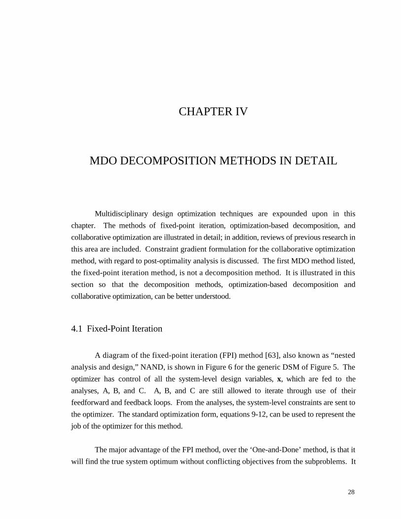
28
CHAPTER IV
MDO DECOMPOSITION METHODS IN DETAIL
Multidisciplinary design optimization techniques are expounded upon in this
chapter. The methods of fixed-point iteration, optimization-based decomposition, and
collaborative optimization are illustrated in detail; in addition, reviews of previous research in
this area are included. Constraint gradient formulation for the collaborative optimization
method, with regard to post-optimality analysis is discussed. The first MDO method listed,
the fixed-point iteration method, is not a decomposition method. It is illustrated in this
section so that the decomposition methods, optimization-based decomposition and
collaborative optimization, can be better understood.
4.1 Fixed-Point Iteration
A diagram of the fixed-point iteration (FPI) method [63], also known as “nested
analysis and design,” NAND, is shown in Figure 6 for the generic DSM of Figure 5. The
optimizer has control of all the system-level design variables, x, which are fed to the
analyses, A, B, and C. A, B, and C are still allowed to iterate through use of their
feedforward and feedback loops. From the analyses, the system-level constraints are sent to
the optimizer. The standard optimization form, equations 9-12, can be used to represent the
job of the optimizer for this method.
The major advantage of the FPI method, over the ‘One-and-Done’ method, is that it
will find the true system optimum without conflicting objectives from the subproblems. It

29
has several disadvantages. The disciplinary experts running the analyses do not have much
say in the optimization process. The system optimizer can become large due to the fact that
it controls all system-level design variables and constraints. A, B, and C must execute
iteratively, consuming more real time than if they executed in parallel. Also, noisy gradients
occur due to the presence of an iteration tolerance, which causes convergence problems.
Figure 6: Generic FPI Diagram
4.2 Optimization-Based Decomposition
The single-level decomposition method, optimization-based decomposition (OBD)
[63], is illustrated in Figure 7. In this method, the feedforward loops and the feedback
loops of the DSM have been broken. Since there is no longer any iteration between the
analyses, the system-level optimizer must take over an additional job of ensuring
compatibility between A, B, and C. The variables that once were represented by the
feedforward and feedback loops, intermediate variables A’, B’, and C’, are now controlled
by the system-level optimizer as additional design variables. Along with the system-level
constraints, the coupling variables calculated by the analyses, A, B, and C, are also passed to
the optimizer. To ensure compatibility between the inputs, A’, B’, and C’, and outputs, A,
B, and C, new constraints, called compatibility constraints are formed. These are additional
constraints on the system level.
The optimizer’s job for OBD can be written in the standard form as follows:

30
Minimize: F(x, A’, B’, C’) x = x1, x2, …xn (13)
Subject to: gj(x, A’, B’, C’) ≤ 0 j = 1, m (14)
hk(x A’, B’, C’) = 0 k = 1,l (15)
xil ≤ xi ≤ xi
u i = 1, n (16)
Al ≤ A’ ≤ Au
Bl ≤ B’ ≤ Bu
Cl ≤ C’ ≤ Cu
where g includes the compatibility constraints, an example of which is given by
equation 17.
gj(x,A)= ||A’ – A|| ≤ 0 (17)
Figure 7: Generic OBD Diagram
Note that the OBD scenario illustrated in Figure 7 is a completely parallel method
with respect to execution of the analyses. Another scenario for OBD is when only the
feedback loops are broken. This is a partial decomposition (POBD) as opposed to the full
decomposition in Figure 7.

31
An advantage of this parallel scheme is that A, B, and C can be run simultaneously,
reducing the execution time even more. This is because there is no iteration (between A, B,
and C) for this method. That coupling is handled by the compatibility constraints.
Disadvantages are that the size of the optimizer can become quite large and system experts
have little say in terms of optimality in their respective analyses.
As stated before, the OBD MDO method has been investigated for various
problems, ranging from mathematical problems to launch vehicle design. In [44], fully
parallel OBD was used to simultaneously optimize an aircraft and its flight path.
Decomposition was achieved on two levels, the flight segments and the disciplinary
analyses. This type of decomposition is referred to as ‘2-dimensional decomposition.’
Specific details for that problem appear in [45]. Fixed-point iteration and the partial OBD
method were used to solve a single-stage-to-orbit launch vehicle in [46]. Comparisons of
the results are included in Section 4.5. In [47], different formulations of the compatibility
constraints are listed and each is used to solve a fully parallelized aircraft design problem.
With a sequential quadratic system-level optimizer, a compatibility constraint posed as in
equation 18 had the highest percentage of converged solutions, while that posed like
equation 19 gave the fastest solutions in terms of CPU time.
x
′ x = 1± ε (18)
x − ′ x ( )2 ≤ ε (19)
In [48], single-level optimization was used to solve the overall minimization of the
weight of the exterior frame of a 50-story building subject to structural constraints.
Approximately12.5 hours of CPU time was required for one iteration. The problem was
solved using collaborative optimization and those results are listed in the next section.
4.3 Collaborative Optimization

32
The collaborative optimization (CO) [50] method, which is illustrated in Figure 8, is
a multi-level decomposition method. For the design represented in the DSM of Figure 5,
the application of the CO method would require optimization at the analysis level (indicated
by the dashed lines in the analysis boxes) and the system level. In this type of
decomposition, the system-level optimizer’s job is to coordinate the subsystems’
optimization while minimizing the overall objective. In addition to the system-level design
variables, the design variables for the system include the coupling variables, now termed
targets, A , B , and C . Each analysis is sent a complete set of its targets, regardless if these
variables are an input or output of the analysis. Each analysis has a local version of the
targets that are selected by the local optimizer or calculated by the analysis.
The system constraints are the sum-squared errors, JA, JB, and JC, between the targets
and the local values from each analysis and any system-level constraints. The objective of
the subsystems is to minimize its respective error, JA, JB, and JC, while satisfying all its
subsystem level (or local) constraints.
Figure 8: Generic CO Diagram
Because the optimization in this method is on two levels, the goals of the
collaborative optimization method can be stated by two standard forms. The system-level
optimization is given by equations 20 – 22.
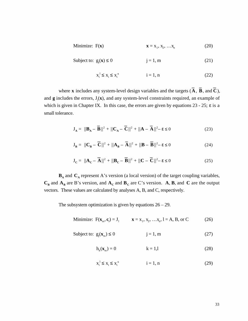
33
Minimize: F(x) x = x1, x2, …xn (20)
Subject to: gj(x) ≤ 0 j = 1, m (21)
xil ≤ xi ≤ xi
u i = 1, n (22)
where x includes any system-level design variables and the targets (A , B , and C ),
and g includes the errors, Jj(x), and any system-level constraints required, an example of
which is given in Chapter IX. In this case, the errors are given by equations 23 - 25; ε is a
small tolerance.
JA = ||BA – B ||2 + ||CA – C ||2 + ||A – A ||2– ε ≤ 0 (23)
JB = ||CB – C ||2 + ||AB – A ||2 + ||B – B ||2– ε ≤ 0 (24)
JC = ||AC – A ||2 + ||BC – B ||2 + ||C – C ||2– ε ≤ 0 (25)
BA and CA represent A’s version (a local version) of the target coupling variables,
CB and AB are B’s version, and AC and BC are C’s version. A, B, and C are the output
vectors. These values are calculated by analyses A, B, and C, respectively.
The subsystem optimization is given by equations 26 – 29.
Minimize: F(xss, cl) = Jl x = x1, x2, …xn, l = A, B, or C (26)
Subject to: gj(xss) ≤ 0 j = 1, m (27)
hk(xss) = 0 k = 1,l (28)
xil ≤ xi ≤ xi
u i = 1, n (29)

34
where xss is the vector of the subsystem’s local design variables, cl is the vector of
the local versions of the coupling targets, both inputs and outputs (like A, BA and CA in
equation 23), and g is the vector of local constraints.
A main advantage of the CO method is that disciplinary experts can control their
own analyses so that the local objective functions (minimizing the errors) and constraints
are met. The system optimizer is relatively small (containing only the target variables,
system-level constraints, and the overall objective function) and A, B, and C execute
simultaneously, conserving time. CO lends itself well to the design process since the
experts’ knowledge is still a part of the subsystem optimization processes which is run in a
time-saving parallel manner. This method, too, finds the true system-level optimum.
Collaborative optimization has some disadvantages as well. There may be coding or
robustness problems given that the analyses have their own optimization problem. This will
also contribute to a greater execution time at the local level.
As previously stated, the CO MDO method has been used in the solutions for
various problems. Just like for OBD methods, these range from mathematical problems to
launch vehicle design problems. References [50] and [54] discuss the development of the
collaborative optimization architecture. In addition, lunar trajectory designs and design of
an SSTO launch vehicle with cost analysis are solved with this architecture [50, 54]. The
lunar trajectory solution was segmented into increasing numbers of paths. When compared
to solutions from a standard approach, the CO method was found to perform better, from a
CPU and objective function standpoint, as the number of segments was increased.
In [51], the comparisons of the different decomposition methods that were used to
solve the SSTO design of [46] are summarized. The addition of the cost analysis is
summarized in [52]. Summaries of these comparisons are given in Section 4.5.
The optimal solution of the sizing of the medium range transport aircraft of [44] is
solved with collaborative optimization in [53]. The aircraft problem of [47] was also solved
with the CO method and comparisons are listed in Section 4.5. CO was used in the design
of a cable-supported bridge in [55]. Two subsystems existed at the sub-level.

35
Nonlinear subspaces can present problems with solution convergence in the CO
method. If multiple solutions exist, the subspace optimizer may ‘jump’ from one solution
to the next creating invalid gradient information at the system-level, thus leading to poor
performance at the system-level. This problem of design space solution sensitivity was
addressed with the introduction of slack variables as the most applicable potential solution
to this problem [50].
Since it is a multilevel decomposition scheme, the CO method results in many
function call and long CPU times at the subsystem level. In more recent years, research has
been performed to reduce these function calls and CPU times. A promising way to achieve
this is through use of response surfaces methods to approximate the optimization at the
subsystem level. This was implemented in the vehicle designs of [57] and HSCT wing
designs of [58] with results incorporated significantly reduced function calls and CPU
times.
All of the previously mentioned solutions with the collaborative optimization method
used the sequential quadratic programming optimization scheme for the system-level
optimization. In [56], CO was used for space based infrared system constellation design.
The system-level optimization scheme in that case was a penalty function method. This was
due to the fact that gradients were not available for the subsystem analysis solutions, which
involved grid search and heuristics in their optimization. However, results were successfully
obtained with this system-level optimization that differed from earlier work.
4.4 Post-Optimality Conditions for Collaborative Optimization
Post-optimal sensitivity analysis can be used to investigate trade-offs in design and
it can also be used in optimization to aid in finding the optimal solution [64, 65]. Basically,
given an optimal solution, post-optimality sensitivity analysis is a useful tool for
investigating the effects, on that solution, of varying a parameter that plays a role in the
analysis. In general, the crux of the analysis is given by Equation 30. The first term
represents the change in the optimal objective function, F*, due to a change in the parameter,
p. The second term is the change in F due to a change in p evaluated at the optimum. In the
third term, g is the constraint vector, x* is the set of design variables at the optimal solution,

36
λ is the Lagrange multiplier vector used to satisfy the Kuhn-Tucker necessary conditions
[25], and r is the set of constraint boundaries, or ε in the previous equations.
dF*
dp=
∂F
∂p
x *
− λT ∂g(x* ,p,r)
∂p(30)
The use of post-optimality sensitivity analysis has been successfully demonstrated
for collaborative optimization [50, 55, 57, and 58]. Expensive gradient function calls can be
eliminated through the knowledge that the subsystems (analyses A, B, and C above) give
optimal solutions at each system-level iteration. These optimal solutions, the sum-squared
errors, Jl, from Section 4.3, are the constraints for the system-level problem. Thus, the
constraint gradients for the system-level optimization problem can be formulated using
post-optimality sensitivity analysis. Equation 31 gives the result when equation 30 is
applied to the subsystem optimal solutions and is true for each optimized subsystem
analysis. For this case, c* is the vector of the local versions of the coupling targets, x, at the
optimum J, and g represents the vector of subsystem constraints.
dJ *
dx i
=∂J *
∂x i
− λT ∂g(xss ,c*,ε)
∂xi
(31)
Since the subsystem constraints, g, are explicit functions of the subsystem variables
(xss and c*) only, the second term of equation 31 becomes zero and equation 32 results
[50]. This result is true for all subsystems and target variables, x.
dJ *
dx i
=∂J *
∂x i
= −2(ci* − xi) (32)
where the generic form of J is
J = ci* − xi( )2
i =1
n
∑ (33)

37
Post-optimality sensitivity analysis will be used for the solutions of the collaborative
optimization schemes of the problems detailed in Chapters VI and VIII. Equation 33 will be
used to calculate the system-level constraint gradients.
4.5 Summary of Decomposition Methods
Several comparisons of decomposition methods exist for aircraft wing design [44,
53], SSTO design [46, 51, and 52], common mathematical problems [49], a civil engineering
building problem [48], and ten coupled problems from diverse design fields [66, 67]. Not
all methods worked for all design problems, so broad generalizations can be made, but may
not be entirely accurate.
For the multidisciplinary wing design problem of [44] and [53], comparisons
between the OBD and CO methods revealed that each solution resulted in the same
optimum. For that problem, the CO method took several hours to complete while the OBD
method was finished in several minutes. In [46], FPI was found to be less computationally
efficient than OBD, which had a smoother design space. For the same problem, CO was
applied in [51]. Lack of subsystem smoothness in the trajectory discipline created
obstacles. That optimizer was taken out and the entire problem was solved in a much
greater amount of time than the solutions of [46]. For a similar problem, [52], which added
cost to the weights and sizing analysis, the CO method was solved with the trajectory
subsystem optimization. It was less computationally efficient than OBD with, on average,
many more function calls. However, computationally, it was at the same level with the FPI
method. For the problem of [52], the CO method exhibited a much faster set-up time than
either the FPI or OBD methods and the communication requirements between the system
and subsystem levels were the least for the CO method.
For some problems, CO was found to have fewer function calls than single-level
decomposition methods and was found to be less robust [67]. In [49], single-level
decomposition techniques were found to be an order of magnitude more computationally
efficient than multi-level techniques for ‘trivial’ problems. However, for a ‘non-trivial’,
highly coupled problem found in building design, collaborative optimization more
computationally efficient [48]. The authors propose that this was due to the facts that the

38
large problem was segmented info many smaller problems, like that of the lunar trajectory
of [50], and that ‘engineering intuition’ was included to simplify the design. More
applications should be tested before any general conclusions can be made regarding the
later reason as this result could be problem dependent.
Table 3 summarizes the characteristics of the four proposed MDO solution
techniques — fixed-point iteration (FPI), two variations of optimization-based
decomposition (OBD), and collaborative optimization (CO). In addition, an entry labeled
‘Manual Iteration’ is included for comparison. Manual Iteration is simply the ‘One-and-
Done’ (sequential) method iterated to ensure that the coupling variables are internally
consistent between the two analyses. The Manual Iteration method is not a preferred
solution however, since the conflict between the competing objective functions of the
contributing analyses is not resolved. The second column of Table 3 refers to whether the
coupled variables are consistent between the analyses at the solution, as is true for all the
methods listed. The fourth and fifth columns are interdependent in that if the system-level
optimizer is not present conflicting objective functions may occur and vice-versa.
Table 3: Proposed MDO Solution Techniques
Method InternallyConsistent
Data
IterationRequiredBetweenAnalyses
Potential forConflictingObjectiveFunctions
RequiresSystem-level
Optimizer
ContributingAnalysisExecution
Optimizer Strategy
Manual Iteration Yes Yes Yes No Sequential Distributed
Fixed PointIteration (FPI)
Yes Yes No Yes Sequential System Level(large)
Partial OBD Yes No No Yes Sequential System Level(very large)
Full OBD Yes No No Yes Parallel System Level(extremely large)
Collaborative Yes No No Yes Parallel Distributed

39
CHAPTER V
THE BRANCHING TRAJECTORY PROBLEM
FORMULATED USING MDO
Since its structure consists of at least two highly coupled subproblems, the
branching trajectory problem resembles more common multidisciplinary problems such as
the coupling between structures and aerodynamics (even though, in this case the
subproblems are actually of the same discipline!). For that reason, solution techniques from
the field of Multidisciplinary Design Optimization (MDO) can be advantageously applied
to its solution. MDO methods have been successfully proposed for and/or used in the
solutions to highly coupled subproblems from a single discipline. These disciplines
include: wing design of the HSCT [58], fluid dynamics [68], and propulsion with respect to
the linear aerospike [69].
This study utilized the Program to Optimize Simulated Trajectories (POST I) in
order to simulate the branching trajectories. In the following figures, the orbital branch will
be designated as ‘Orbit.’ The flyback branch will be denoted as ‘Flyback.’ The ascent
trajectory will be labeled ‘Ascent.’ When the internal optimization capability in POST is
enabled, a box with a diagonal line will indicate that POST is being used for trajectory
analysis plus local optimization. A plain box will indicate that POST is simply being used
to integrate along a given trajectory.

40
5.1 The Fixed-Point Iteration Method
In the FPI method of Figure 9, the system optimizer has control of all trajectory
variables and constraints. Each trial step from the system optimizer requires a series of
iterations between Ascent, Orbit, and Flyback. Given guesses for upper stage and flyback
fuel weights and its initial trajectory variables from the optimizer, Ascent runs in non-
optimizing mode (i.e. it simply integrates the equations of motion along the given trajectory
and returns the results). The resultant staging vector (Ps ) is then input to Orbit and
Flyback. With these initial conditions as a starting point and their subset of trajectory
variables from the system optimizer, Orbit runs in non-optimizing mode, followed by
Flyback. The new upper stage weight, wus, and the new flyback weight, wfb, are fed back to
Ascent through a resizing process. The iterations between Ascent, Orbit, and Flyback
continue until the convergence criterion is met to within a certain tolerance. After the
iteration process is completed, the outputs from each POST analysis are fed back to the
system optimizer to determine the objective function and system constraints. The control
variables are then changed in order to minimize/maximize the system-level objective.
Figure 9: FPI for Branching Trajectories

41
Figure 10: POBD for Branching Trajectories
5.2 The Optimization-Based Decomposition Methods
The optimization-based decomposition methods also require a system optimizer
with an objective function to optimize the system-level objective. In the partial OBD
method, the feedback loops from Orbit and Flyback to Ascent in the FPI method are
broken. Two additional design variables for Ascent are now needed to replace the weights,
which were originally fed back. These are the prescribed upper stage weight, wus ', and the
prescribed flyback fuel weight, wfb', which are controlled by the system-level optimizer. Two
compatibility constraints added to the system optimizer are used to ensure agreement
between the prescribed weights and the true weights output from Orbit and Flyback at the
solution. As a result, iteration is no longer required between Ascent, Orbit, and Flyback to
ensure data consistency. A diagram of this method can be seen in Figure 10. The booster
will be resized, as a function of the flyback fuel requirement, during the optimizer’s
execution.
In the full OBD method of Figure 11, both the feedback and the feedforward loops
that can be seen in the FPI method diagram are broken. In addition to the new design
variables and compatibility constraints from the broken feedback loops (defined in the
previous paragraph), a set of intermediate variables representing the prescribed staging
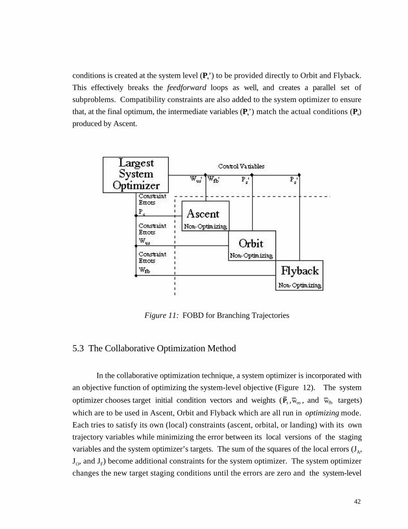
42
conditions is created at the system level (Ps’) to be provided directly to Orbit and Flyback.
This effectively breaks the feedforward loops as well, and creates a parallel set of
subproblems. Compatibility constraints are also added to the system optimizer to ensure
that, at the final optimum, the intermediate variables (Ps’) match the actual conditions (Ps)
produced by Ascent.
Figure 11: FOBD for Branching Trajectories
5.3 The Collaborative Optimization Method
In the collaborative optimization technique, a system optimizer is incorporated with
an objective function of optimizing the system-level objective (Figure 12). The system
optimizer chooses target initial condition vectors and weights (P s ,w us , and w fb targets)
which are to be used in Ascent, Orbit and Flyback which are all run in optimizing mode.
Each tries to satisfy its own (local) constraints (ascent, orbital, or landing) with its own
trajectory variables while minimizing the error between its local versions of the staging
variables and the system optimizer’s targets. The sum of the squares of the local errors (JA,
JO, and JF) become additional constraints for the system optimizer. The system optimizer
changes the new target staging conditions until the errors are zero and the system-level

43
objective function is optimized. In this method, the resizing event will occur during the
system optimizer execution.
Figure 12: CO for Branching Trajectories

44
CHAPTER VI
THE FIRST APPLICATION: THE KISTLER K-1
LAUNCH VEHICLE
To provide applicability to this research, the missions of two candidate TSTO launch
vehicle designs have been chosen to serve as reference missions. In this chapter, the Kistler
K-1 launch vehicle is described. The results for this application are analyzed in Chapter
VII. In Chapters VIII and IX, the second application and its results, respectively, are
reported.
6.1 The Kistler K-1 Launch Vehicle
Many launch vehicles are currently being developed by commercial industries with
the goal of capturing a profitable share of the growing satellite launch market. Such is the
case of the Kistler K-1 launch vehicle [70, 71]. The K-1 (Figure 13, [72]) will be a fully
reusable, two-stage vehicle that incorporates branching trajectories. The vehicle’s booster
will use three Aerojet modified NK33 engines [73, 74]. The K-1’s upper stage will be
propelled by one Aerojet modified NK43 engine [73, 74]. There will be different versions
of the vehicle to accommodate various payload classes. One of its missions will be to
deliver a certain payload to a 50 nmi x 846 nmi x 51˚ orbit. This is the mission that will be
analyzed in this study.

45
The data (weights, trajectory constraints, engine data, etc.) pertaining to the
aforementioned mission was provided directly by Kistler Aerospace [75]. An outline of the
weights used, dry and propellant weights, for both stages are listed in Appendix A.
As mentioned in Section 2.4, POST requires inputs to evaluate the aerodynamics of
a vehicle. The tool, Aerodynamic Preliminary Analysis System, APAS [76], was used to
generate the aerodynamic data for this problem. In particular, for this case, three sets of
aerodynamic data were generated. A table of lift, drag, and moment coefficients, as a
function of Mach number and angle of attack, was created for each of the three
configurations for the K-1: the vehicle as a whole, the booster by itself, and the upper stage
by itself. Appendix B lists more detailed information about the aerodynamics for the K-1.
POST also requires propulsion data input. Also contained in Appendix B is information
about the engines’ performance for the K-1.
Figure 13: The K-1

46
Figure 14: The K-1 Flight Profile
6.2 The Kistler K-1 Trajectory
The trajectory of the K-1 launch vehicle can be seen in Figure 14 [72]. It will
consist of an RTLS type branching trajectory as in Figure 1. After launch from the site at
Woomera, Australia, (1) the entire K-1 will fly until staging approximately 120 seconds later
(2). After staging, the booster performs a pitcharound maneuver that will guide itself back
to within 10,000 ft of the launch site, to land with airbags and parachutes. The upper stage
will continue on to the designated orbit (3). For the purposes of this study, the simulation
will end when the orbital targets have been attained. In reality, after expulsion of the
payload (4) the K-1’s upper stage will deorbit (5) and return to the launch site (6).

47
Figure 15: The DSM for the K-1
The trajectory is simulated through two POST decks as indicated by the DSM for
the K-1’s trajectory as shown in Figure 15. The first POST deck follows the vehicle from
launch to orbital injection of the upper stage. Note that this specific simulation combines
the Ascent and Orbit jobs. The second, or flyback branch, follows just the booster from
staging to its return to the launch site. In addition to a three-degree-of-freedom simulation,
each POST deck uses the following modeling options: 1976 standard atmosphere, lift and
drag aerodynamic coefficients, fourth order Runge-Kutta integration with a one second
integration step size, and a spherical Earth approximation.
Table 4: POST Controls and Constraints for the K-1
POST
Deck
Number of Independent
Variables
Number of
Constraints
Ascent 13 5
Flyback 6 2
Total 19 7
Table 4 lists the number of controls and constraints used by the ascent and flyback
trajectory decks. The reference K–1 ascent trajectory deck’s independent variables are
twelve pitch angles and payload weight. The ascent has five constraints involving orbital
insertion criteria and dynamic pressure boundaries. The vehicle is steered by a table look-

48
up of inertial pitch angles. Nominally, the objective of the orbital branch is to maximize the
payload for a given set of propulsion characteristics, vehicle aerodynamics, K-1 weights, and
ascent propellant.
The reference flyback trajectory deck uses six independent variables: four pitch
angles, azimuth of the pitcharound maneuver needed to initially head the vehicle in a
direction back to the launch site, and engine burn time. The two constraints guarantee a
smooth rocket pull-up and landing within a certain downrange distance. Given a set of
engine propulsion characteristics, aerodynamics, and a staging point, the flyback trajectory
nominally tries to minimize flyback fuel weight. The required staging point data from the
ascent branch includes altitude, flight path angle, latitude, longitude, velocity, and velocity
azimuth. The booster is steered initially by an angle of attack of 180 degrees used to head
the vehicle back to the launch site. The turnaround maneuver is achieved with pitch angle
steering.
6.3 The Objective Function for the Kistler K-1
Note that there are many ways to optimize the trajectories of both the upper stage
and the booster. Should the booster ascent propellant be resized if necessary? Should all
inert weights remain fixed? Should the system-level objective be maximum orbital payload
or minimum booster weight?
For the K-1 simulation, fixed weights were used for all weights except for booster
ascent propellant weight, flyback fuel weight, and payload weight. Consequently, the
exterior of the vehicle stayed the same throughout thus did the aerodynamics as well. The
constant total propellant weight, given by equation 34, was the sum of the booster ascent
propellant weight and the flyback fuel weight used. (Note that pre-liftoff propellants are
subtracted from the total propellant.) This equation was very easily coded into the system-
level optimizer. The payload weight was the objective to be maximized.
487,823 lbs = ascent_propellant + flyback_propellant (34)
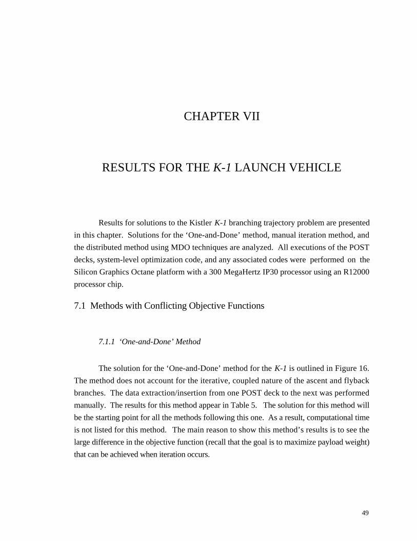
49
CHAPTER VII
RESULTS FOR THE K-1 LAUNCH VEHICLE
Results for solutions to the Kistler K-1 branching trajectory problem are presented
in this chapter. Solutions for the ‘One-and-Done’ method, manual iteration method, and
the distributed method using MDO techniques are analyzed. All executions of the POST
decks, system-level optimization code, and any associated codes were performed on the
Silicon Graphics Octane platform with a 300 MegaHertz IP30 processor using an R12000
processor chip.
7.1 Methods with Conflicting Objective Functions
7.1.1 ‘One-and-Done’ Method
The solution for the ‘One-and-Done’ method for the K-1 is outlined in Figure 16.
The method does not account for the iterative, coupled nature of the ascent and flyback
branches. The data extraction/insertion from one POST deck to the next was performed
manually. The results for this method appear in Table 5. The solution for this method will
be the starting point for all the methods following this one. As a result, computational time
is not listed for this method. The main reason to show this method’s results is to see the
large difference in the objective function (recall that the goal is to maximize payload weight)
that can be achieved when iteration occurs.

50
Table 5: ‘One-and-Done’ and Manual Iteration Method Results (K-1)
Method PayloadWeight (lbs)
POST ComputationalTime
Number ofIterations
‘One-and-Done’ 3314.7881 - 0
Manual Iteration 3528.7911 201.4 sec (3.36 min) 6
Figure 16: ‘One-and-Done’ Method Flowchart, K-1
For this method, the initial guess for booster ascent propellant is significant. The
percentage of booster ascent propellant, with respect to the total available, used for this
simulation was 92.88%. This left a little more than 7% for the flyback fuel. After the serial
execution of the two POST decks, it was found that 14.6% of the initial flyback fuel was left
over, or not used. If the guess for booster ascent propellant percentage was too high, then
the possibility of not having enough flyback fuel would have existed. In that case, as far as
the flyback simulation is concerned, the constraints would have been met, however, negative
propellant would be used. In other words, the POST deck would have used the dry weight

51
as propellant, resulting in an obviously wrong answer. That scenario highlights an example
of one of the many deficiencies of this method.
As stated previously, the next method and the MDO methods will all begin with the
solution to the ‘One-and-Done’ method. Thus, the initial guesses are as follows:
percentage of flyback fuel – 6.08% (the original initial guess less 14.6% of that guess,
resultant percentage of booster ascent propellant – 93.92%, and payload weight – 3,314.79
lbs.
7.1.2 Manual Iteration Method Results
The manual iteration method uses two subproblem optimizers and no system-level
optimizer. A flowchart of the method can be seen in Figure 17. Execution is sequential and
iterative between the ascent deck and the flyback deck. The flyback weight is updated as the
iterations occur. Again the data extraction/insertion is manual. Iteration information and
execution time results are shown in Table 5. For this case, iteration was performed between
the two basic subproblems to ensure data consistency (unlike the ‘One-and-Done’ method),
however the conflicting objective functions were not addressed. The convergence criterion
for the manual iteration method was flyback fuel weight. The K-1 was considered
converged when this variable came within .01% of the result from the previous iteration.
This result will be used as a comparison case in the MDO method assessments. The final
design variables used for this method are listed in Appendix C.

52
Figure 17: Manual Iteration Method Flowchart, K-1
7.2 The System-Level Optimizer
The Design Optimization Tool, DOT™ [77], is a commercial optimization program
that is supplied without charge for academic research. It provides several algorithms for
optimization that have been used to generate the results for the MDO methods. The
program contains optimization methods for constrained and unconstrained problems. For
branching trajectories, the MDO methods used result in constrained problems. The
available algorithms are: modified method of feasible directions (MMFD), sequential linear
programming (SLP), and sequential quadratic programming (SQP). Each uses gradient
information to find a new direction to look for the optimal solution. The new direction for
MMFD, or search direction, is based on lowering the constraint violation while minimizing
the objective function. For the SLP and SQP methods, Taylor Series approximations of the
objective function and constraints are used in optimization. The SLP method solves the

53
linear approximate optimization problem. The SQP method solves the optimization
problem using a search direction based on the quadratic approximate problem optimization
problem with linearized constraints.
7.3 Multidisciplinary Design Optimization Results
Table 6 shows the system optimizer size for the K-1 case. DOT™ requires that
equality constraints be formulated as inequality constraints. The equality constraints for all
the POST decks were posed as two inequality constraints. Three of the constraints from
Table 4 were equalities; formulated as inequality constraints, this brings the total number of
constraints for the FPI method to ten. Note that for the POBD method, there were either
one or two more constraints in addition to those of the FPI method. The compatibility
constraint can be posed as either a squared inequality constraint (eleven total constraints,
equation 35) or two inequality constraints (twelve total constraints, equation 36.) The
compatibility constraints for the full OBD method were posed as seven pairs of inequality
constraints, thus the total number of constraints was twenty-four. Note that the
compatibility constraints, like all the other constraints, are normalized to aid in the numerical
conditioning of the problem.
Table 6: Size of System Optimizer for Kistler K-1 Cases
Variables Constraints
Manual Iteration - -
FPI 19 10
Partial OBD 20 12/11
Full OBD 26 24
Collaborative 8 2
gi =fbw − fbw'
10,000
2
≤ 0 (35)

54
gi, i+1 = ±fbw − fbw'
10,000
≤ 0 (36)
It is imperative to note that while the number of target variables for the collaborative
optimization scheme is expected to be seven (flyback fuel weight plus the six staging vector
components), eight appear in Table 6. This will be expounded upon in Section 7.3.4.
7.3.1 Fixed-Point Iteration Method
The flowchart for the FPI method can be seen in Figure 18. The entire process,
including data extraction/insertion and gradient calculation was automated. The ‘grayed’
boxes in the figure represent those parts of the process that were coded in C++ such as the
main execution program of the optimizer. Data extraction/insertion was achieved with
PERL (Practical Extraction and Report Language) and is represented, in the figure, by
dashed arrows. The system-level optimizer used was the Modified Method of Feasible
Directions.
The Fixed Point Iteration method involves use of a system-level optimizer and
POST deck iterations. The POST decks are not optimized for this method. They are used
to integrate the equations of motion using the set of controls given by the system-level
optimizer. The POST deck iterations were considered converged when the flyback fuel
weight was within 0.01% of itself, just like in the manual iteration method. The gradients
for the system-level optimizer were calculated using central finite differences with varying
perturbation sizes that were dependent on the size and type of the original design variable.
Quantitative results for this method were obtained using the optimization scheme of
the Modified Method of Feasible Directions and detailed results can be seen in Tables 8 &
9 in Section 7.4. The FPI method gave an optimized solution of 3,544 pounds of payload
weight in 16.3 minutes with eighteen system-level iterations. Appendix C lists the final set
of design variables for this method. Figure 19 shows how the payload weight varied with
function call. In addition, the plot shows the number of MMFD iterations, the line searches
needed to define the search direction, per function call. Figure 20 shows the log of the

55
active constraints at each MMFD iteration. Active constraints are those that were either
violated or greater than –0.5.
In Figure 20, the line denoting the ‘feasible solution’ was found by calculating the
log of the 2-norm of the accepted tolerances of the active constraints. For example, all of
the constraints for the FPI method were scaled such that a single tolerance, ε, of 0.0001 was
used for all the constraints. If ‘n’ constraints were active, the equation used for the feasible
solution at iteration one would be that of equation 37. The ‘feasible solution line for all
MDO methods was similarly calculated based on the number of active constraints, n, and
acceptable tolerances, ε.
log nε 2( ) (37)

56
Figure 18: FPI Flowchart, K-1

57
3300
3350
3400
3450
3500
3550
3600
0 20 40 60 80 100
Function Call
0
2
4
6
8
10
12
14
16
18
20
Payload Weight (lbs)
MMFD Iteration Number
Figure 19: Payload Weight Tracking for FPI Method
-4.5
-4
-3.5
-3
-2.5
-2
-1.5
-1
-0.5
00 2 4 6 8 10 12 14 16 18 20
3300
3350
3400
3450
3500
3550
3600
log(||gi||)Feasible SolutionPayload Weight
Figure 20: Active Constraint History for the FPI Method
MM
FD Iteration N
umber
Payl
oad
Wei
ght (
lbs)
Payload Weight (lbs)
Log
||g i
||
Function Call
System-Level Iteration

58
7.3.2 Partial Optimization-Based Decomposition
The flowchart for the POBD methods, with the compatibility constraint posed as
either one or two inequalities as described in Section 7.3, can be seen in Figure 21. For
these methods, the compatibility constraint is needed for the flyback fuel weight only.
Like the FPI method, the POBD methods involve use of a system-level optimizer
and POST decks that are not optimized, however, feedforward of the staging vector still
exists. The gradients for the system-level optimizer for these methods were also calculated
using central finite differences with a varying perturbation size. Again, the entire process,
including data extraction/insertion and gradient calculation was automated. Those parts of
the process that required a C++ program are shown as gray boxes in Figure 21. Data
extraction/insertion was achieved with PERL and is indicated by dashed arrows in the
figure.
The system-level optimizer was the MMFD for these methods as well. The POBD
methods resulted in an optimized payload weight of 3,567 pounds in twenty system-level
iterations requiring 15.7 minutes. Detailed numerical results are listed in Tables 8 & 9 in
Section 7.4. Appendix C lists the final set of design variables for this method. Figure 22
shows how the payload weight changed at each function call. Additionally, the plot shows
the number of MMFD iterations per function call. Figure 23 shows the log of the active
constraints at each MMFD iteration. Data for the POBD method that had the flyback fuel
weight compatibility constraint posed as two inequalities is shown in Figures 22 & 23; the
data for the POBD method that had the flyback fuel weight compatibility constraint posed
as one inequality was nearly identical.

59
Figure 21: POBD Flowchart, K-1

60
3300
3350
3400
3450
3500
3550
3600
3650
0 10 20 30 40 50 60 70 80 900
2
4
6
8
10
12
14
16
18
20
Payload Weight MMFD Iteration Number
Figure 22: Payload Weight Tracking for POBD Methods
-4
-3.5
-3
-2.5
-2
-1.5
-1
-0.5
00 2 4 6 8 10 12 14 16 18 20
3300
3350
3400
3450
3500
3550
3600
log(||gi||)Feasible SolutionPayload Weight
Figure 23: Active Constraint History for the POBD Methods
MM
FD Iteration N
umber
Payl
oad
Wei
ght (
lbs)
Payload Weight (lbs)
Log
||g i
||
Function Call
MMFD Iteration Number

61
7.3.3 Full Optimization-Based Decomposition
Figure 24: FOBD Flowchart, K-1
The flowchart for the FOBD method, with the compatibility constraints posed as
pairs of inequalities as described in Section 7.3, can be seen in Figure 24. There are seven
compatibility constraints needed for this method: flyback fuel weight and the staging vector

62
of altitude, velocity, azimuth velocity, flight path angle, latitude, and longitude. All of these
constraints are normalized in the problem set-up.
The FOBD method requires the use of a system-level optimizer and POST decks
that do not themselves optimize. For this method, there is no feedback or feedforward and
the POST decks are executed in parallel. The gradients for the system-level optimizer for
this method were also calculated using central finite differences with a varying perturbation
size. The entire process, including data extraction/insertion and gradient calculation was
automated. Those parts of the process that required a C++ program are shown as gray
boxes in Figure 24. Data extraction/insertion was achieved with PERL and is indicated by
dashed arrows in the figure.
3300
3400
3500
3600
3700
3800
3900
4000
4100
0 20 40 60 80 100
Function Call
0
5
10
15
20
25
30
35
Payload Weight (lbs)MMFD Iteration Number
Optimization Restart
Figure 25: Payload Weight Tracking for the FOBD Method
The system-level optimizer was the MMFD for the FOBD method. The
optimization had to be restarted once due to a lack of progress the first time. After this
restart, an optimal solution of 3,585 pounds of payload weight was found. This took about
sixteen minutes total in thirty-four system-level iterations for the entire problem.
Quantitative results are listed in Tables 8 & 9 in Section 7.4. Appendix C lists the final set
Payl
oad
Wei
ght (
lbs)
MM
FD Iteration N
umber

63
of design variables for this method. Figure 25 shows how the payload weight changed at
each function call. Additionally, the plot shows the number of MMFD iterations per
function call. Figure 26 shows the log of the active constraints at each MMFD iteration.
-4
-3.5
-3
-2.5
-2
-1.5
-1
-0.5
00 5 10 15 20 25 30 35
3300
3350
3400
3450
3500
3550
3600
3650
log(||gi||)Feasible SolutionPayload Weight
Figure 26: Active Constraint and Objective History for the FOBD Method
7.3.4 Collaborative Optimization
Figure 27 shows the flowchart for the CO method. The CO method involves the
use of a system-level optimizer and a parallel analysis structure. However, for this multi-
level decomposition scheme, the POST decks are optimized using the NPSOL optimizer
included in the POST software.
The entire process, including data extraction/insertion and gradient calculation was
automated. Those parts of the process that required a C++ program are shown as gray
boxes in Figure 27. Data extraction/insertion was achieved with PERL and is indicated by
dashed arrows and box lines in the figure. The dashed lines in the analysis (POST) boxes
indicate that the POST optimizer is in use. After each gradient call, the local POST design
Payload Weight (lbs)
Log
||g i
||
System-Level Iteration

64
variables are copied into the corresponding POST decks as the new controls. This was
done in an effort to minimize the number of function calls required at the subsystem level.
The CO method gave an optimal solution of 3,569 pounds of payload weight. This was
attained in seven system-level iterations requiring 1.84 hours. More results are given in
Section 7.4.
Figure 27: CO Flowchart, K-1

65
There were eight target variables required for this method. These included the
payload and flyback fuel weights and the six variables that composed the staging vector.
Table 7 shows how these target variables were perceived by the ascent and flyback POST
decks, as either inputs or outputs. The system-level constraints, or J’s, were calculated
accordingly.
Table 7: Targets’ Relationship to POST Decks for K-1
Ascent Deck Flyback Deck
Payload Weight Input -
Flyback Fuel Weight Input Output (as a function of Eqn. 26)
Staging Altitude Output Input
Staging Velocity Output Input
Staging Azimuth Velocity Output Input
Staging Flight Path Angle Output Input
Staging Latitude Output Input
Staging Longitude Output Input
Constraint gradient calculations were performed using the post-optimality sensitivity
analysis introduced in Section 4.4. The benefit from this analysis, in that numerous
analysis calls can be eliminated, is exploited if the objective function gradient can also be
calculated analytically. This can be achieved by adding the objective function, in this case,
payload weight, to the vector of targets. In addition, it is now included in the error, J, for the
ascent deck and is perceived as an output from the ascent deck (but an input/control in the
ascent deck). Consequently, the objective function gradient can now be easily and
analytically derived. This target’s inclusion in the flyback deck is not required since it is
neither an input nor an output for that analysis.
Figure 28 shows how the payload weight varied per system-level function call. This
plot also shows how the payload weight from the ascent deck follows the payload weight
target. They are matched almost exactly because the payload weight is a control, or

66
dependent variable, in the POST deck and it can easily be changed to meet the target
requirement.
3250
3300
3350
3400
3450
3500
3550
3600
3650
0 10 20 30 40 50 600
1
2
3
4
5
6
7
Ascent Target System-Level Iteration
Figure 28: Payload Weight Tracking for the CO Method
Figure 29 illustrates the active constraint history for the seven system-level iterations
needed to solve this problem. Because the initial targets came from the solution to the
‘One-and-Done’ method, the first iteration (zero on the graph) was a feasible solution at the
system level. After this iteration, all other iterations then had a feasible solution.
Figures 30 and 31 show the subsystem level target achievement for the first three
system-level iterations (0, 1, and 2) for the ascent propellant and payload weight,
respectively. . The number of subsystem iterations is indicated by the number scale on the
x-axis. The flyback deck was usually very flexible in finding a feasible solution. In Figure
30, the ascent propellant weight was matched at the beginning of the flyback deck’s
iterations and is difficult to see in the plot. In Figure 31, it is shown that the payload weight
increased at every iteration. This was allowed because the ascent deck optimization matched
the target at each iteration.
Pay
load
Wei
ght (
lbs)
Iteration Num
ber
System-Level Function Call

67
-6.25
-6.2
-6.15
-6.1
-6.05
-6
-5.95
-5.9
-5.85
-5.80 1 2 3 4 5 6 7
3300
3350
3400
3450
3500
3550
3600
log||gi|| Feasible Payload Weight
Figure 29: Active Constraint History for the CO Method
452000
453000
454000
455000
456000
457000
458000
459000
460000
1 5 9 13 17 21 25 29 33 37 41 45 49
Target
Ascent
Flyback
5 10 15 20 5 10 5 10 15
Figure 30: System-Level Coordination for Ascent Propellant
Log
||gi||
Payload W
eight (lbs)
System-Level Iteration
Iteration 1 Iteration 2 Iteration 3
Prop
ella
nt W
eigh
t (lb
s)

68
3280
3300
3320
3340
3360
3380
3400
3420
3440
3460
1 6 11 16 21 26 31 36 41 46 51
Target Ascent
5 10 15 20 5 10 5 10 15
Figure 31: System-Level Coordination for Payload Weight
7.4 Summary
Tables 8 and 9 give quantitative results for the Kistler K-1 MDO methods. In Table
8, POST computational time refers to the total amount of time to run the POST decks for all
calls, including function calls and gradient calls. Although the actual method executions
were performed with one processor, the CPU time results are reported as if two processors
had been available (for example, in the FOBD and CO results, times are given as if the
ascent POST deck ran on one processor while the flyback POST deck ran on another
processor).
As indicated in Table 8, all methods increased the payload weight of the K-1. The
fixed-point iteration method improved the payload weight by about 15 pounds. The partial
optimization-based decomposition improved the payload weight of the K-1 by
approximately 23 pounds over the FPI method. The full optimization-based decomposition
results in about a 42 pound increase in the payload weight over the FPI method. Use of the
collaborative optimization method increased the payload by approximately 32 pounds. The
decomposition methods gave an approximate 40 – 55 pound increase over the manual
Iteration 1 Iteration 2 Iteration 3
Payl
oad
Wei
ght (
lbs)

69
iteration method, a 1.6% increase, which is relevant considering the high costs per pound to
launch payloads.
Table 8: K-1 Results Comparison (MDO)
Method Optimized
Payload Weight (lbs)
POST Computational
Time
FPI 3,543.64 976.8 sec (16.3 min)
POBD 1 3,566.82 939.52 sec (15.7 min)
POBD 2 3,566.85 941.44 sec (15.7 min)
FOBD 3,585.06 968.33 sec (16.1 min)
CO 3,569.04 5,008 sec (1.39 hr)
It was expected that the FPI, POBD, FOBD, and CO methods would result in the
same objective function; however, the lack of performance by the FPI method may be
attributed to the numerical noise introduced by the flyback fuel weight convergence
tolerance on the internal POST iterations. This noise also affects the gradient calculations
for the engine-on time design variable because for that gradient, internal POST iterations
occur. This tolerance then affects the flyback fuel weight and consequently the optimized
payload weight. The marked difference in the FOBD method may partially be attributed to
the existence of tolerances for the staging vector since the feedforward no longer existed.
These tolerances would have affected the final payload weight. The variance in optimum
design variables can be seen in Appendix C.
Some definitions for the columns in Table 9 are required. The third column, ‘POST
calls,’ refers to how many times an analysis evaluation occurred, including system-level,
gradient (except for the CO method), and line search evaluations. For the FPI and POBD
methods one ‘POST call’ is a sequential execution of both POST decks. For the FOBD
method, one ‘POST call’ is a parallel execution of the two POST decks. Note that there are
two numbers given for the CO method. The first is the number of simulation function calls
for the ascent deck, the second is for the flyback deck. As would be expected the number of

70
‘POST calls’ for the collaborative optimization method is significantly larger than that for
the other methods because many function calls were needed for optimization. While the
number of system-level iterations is smaller for CO, many function calls with the
subsystems at each iteration were required.
Table 9: K-1 Detailed Results Comparison (MDO)
Method System-
Level
Iterations
POST Calls Average CPU Time
per
POST Call
Gradient
Calls
FPI 18 884 1.105 sec 17
POBD 1 20 843 1.114 sec 19
POBD 2 20 843 1.117 sec 19
FOBD 34 1622 0.911 sec 29
CO 7 2271/4745 1.326 min 5
In the fourth column, CPU time refers to the average time it took for one POST call
to run, be that iteratively, sequentially, or in a parallel manner. At first glance, the average
CPU times per function call listed in Table 9 are not what one would expect. The average
time for the FPI method is usually larger than that for the OBD methods because the
internal iterations for convergence are many. For the Kistler case, internal convergence
occurred in zero or one iteration, usually zero for gradient calculation (this is because the
flyback fuel weight is controlled by ‘engine-on’ time, one of the design variables). Thus
for the majority of ‘POST calls’, one POST call for the FPI method would take
approximately the same amount of time as one POST call for the POBD method. This is
the case as shown in Table 9. The time for the FOBD method was smaller since the POST
decks were executed in a parallel manner. The Ascent POST deck required a longer amount
of execution time than that of the Flyback deck. Even though the POST decks for the CO
method were executed parallelly, the CPU time was longer because the optimization of the
POST decks required a longer amount of time than a simple integration of the equations of

71
motion did. Gradient calls’ refers to how many times the objective and constraint gradient
vectors were calculated in their entirety.
Note that the results for the POBD method were the same regardless of which way
the compatibility constraints were posed. This was not the case, however, for the FOBD
method. When the compatibility constraints were formed as one inequality per design
variable, a feasible solution was not found.
More quantitative results can be seen in Table 10, which shows the difference in
staging vectors for the methods. Included for comparison is the staging vector for the
manual iteration method. Since the results for the two POBD methods were almost exactly
the same, just one is included in the table. Assuming that convergence tolerances affect the
FPI method staging vector, the results from the other MDO methods imply that a smaller
flight path angle can lessen flyback fuel weight consumed and thus, the increase the payload
weight. (In the FOBD case, the lower staging altitude also has a similar effect.) The
returning booster desires this lower angle so that it can perform its pitcharound maneuver
more efficiently.
Table 10: Staging Vector Results for the K-1
MIM FPI POBD 2 FOBD CO
Altitude, ft 138,028 138,019 138,014 137,542 138,028
Velocity, ft/s 4,172.28 4,169.27 4,166.92 4,160.34 4,171.15
Gamma, deg 33.337 33.520 33.272 32.892 32.667
Vel. Azimuth, deg 43.519 43.517 43.520 43.527 43.526
Latitude, deg -30.893 -30.893 -30.893 -30.900 -30.902
Longitude, deg 137.029 137.028 137.027 137.020 136.996
Figures 32, 33, and 34 show plots of the trajectory data for the different MDO
methods. Through the ascent, the trajectories are very similar with regards to altitude and
velocity. In fact, as can be seen in Table 10, the staging points are relatively close to one

72
another. The angles of velocity azimuth, latitude, and longitude are expected to be identical
considering there are no yawing movements during the ascent and the results of the table
recognize that fact. In Figure 32, it is shown that the flyback altitudes, especially, exhibit
differences. Differing pitch angles during the flyback pitcharound maneuver affect the
flyback trajectory seen in Figure 33, as does the staging altitude.
0
50000
100000
150000
200000
250000
300000
350000
0 50 100 150 200 250 300 350 400
MIM
POBD
FOBD
CO
Figure 32: Altitude versus Time for the K-1
The velocity plot of Figure 34 illustrates the flyback engine-on phase well. For all
methods, from about 130 seconds to 155 seconds the engine is on and the pitcharound to
the launch site occurs. A slight dip in the velocity after the pitcharound occurs as the vehicle
attains a zero degree angle of attack for its ballistic entry. The lowest velocity corresponds
to the highest altitude, after which point the vehicle speeds up as it is aided by gravity as it
descends. Terminal conditions on velocity for the flyback were not imposed.
Alti
tude
(ft
)
Time (sec)

73
-100
-80
-60
-40
-20
0
20
40
60
80
1000 50 100 150 200 250
Time (sec)
MIM
POBD
FOBD
CO
Figure 33: Flyback Pitch Angle versus Time for the K-1
0
5000
10000
15000
20000
25000
30000
0 50 100 150 200 250 300 350 400
MIM
POBD
FOBD
CO
Figure 34: Velocity versus Time for the K-1
Pitc
h A
ngle
(de
g)V
eloc
ity (
ft/s
ec)
Time (sec)

74
CHAPTER VIII
STARGAZER: THE SECOND APPLICATION
8.1 Stargazer
Figure 35: Stargazer Concept
The second application, which uses branching trajectories, is the Stargazer launch
vehicle (Figure 35, [78]). The mission for this vehicle is to deliver a 300 pound payload (of
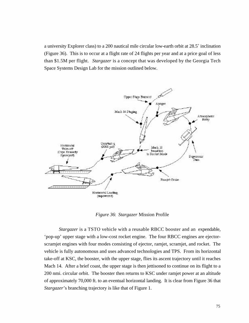
75
a university Explorer class) to a 200 nautical mile circular low-earth orbit at 28.5˚ inclination
(Figure 36). This is to occur at a flight rate of 24 flights per year and at a price goal of less
than $1.5M per flight. Stargazer is a concept that was developed by the Georgia Tech
Space Systems Design Lab for the mission outlined below.
Figure 36: Stargazer Mission Profile
Stargazer is a TSTO vehicle with a reusable RBCC booster and an expendable,
‘pop-up’ upper stage with a low-cost rocket engine. The four RBCC engines are ejector-
scramjet engines with four modes consisting of ejector, ramjet, scramjet, and rocket. The
vehicle is fully autonomous and uses advanced technologies and TPS. From its horizontal
take-off at KSC, the booster, with the upper stage, flies its ascent trajectory until it reaches
Mach 14. After a brief coast, the upper stage is then jettisoned to continue on its flight to a
200 nmi. circular orbit. The booster then returns to KSC under ramjet power at an altitude
of approximately 70,000 ft. to an eventual horizontal landing. It is clear from Figure 36 that
Stargazer’s branching trajectory is like that of Figure 1.

76
8.2 The Design Structure Matrix for Stargazer
Stargazer was initially designed using a collaborative, multidisciplinary integrated
design team approach. Team members executed individual disciplinary analysis tools in an
iterative conceptual design process, exchanging information and data files, for each
candidate configuration, until the propellant mass fractions for each mission segment were
converged. The overall DSM for the Stargazer design process can be seen in Figure 37.
The bolded box represents the main disciplinary iteration loop, the details of which are
shown in Figure 38.
Figure 37: Stargazer DSM

77
Figure 38: Main Iteration Loop
As introduced in Chapter III, the DSM is a useful mechanism for showing the data
interdependencies in a multidisciplinary design process. The main iteration loop exhibits
strong coupling among the propulsion, performance (trajectory optimization) and weights &
sizing disciplines. The aeroheating (thermal protection system) discipline is rather weakly
coupled with the other three beyond the first iteration.
Traditionally, the first two disciplines in Figure 37 iterate to find a feasible
packaging and aerodynamic configuration. Once a feasible configuration is determined, the
analyses in Figure 38 iterate to find a converged, properly scaled design to deliver the 300
lb. payload. (Note that photographic scaling is used such that the aerodynamic coefficients
are the same for a single configuration, only scaled by wing planform area.) The operations
and economics disciplines in Figure 37 are analyzed after a converged design is created.
For this research, however, the emphasis was on the performance discipline alone.
Nonetheless, the other disciplines still play a role. In order to focus on the trajectory, an
initial vehicle had to be baselined. The baseline packaging and configuration is that which is
described in [78]. Figure 39 shows the vehicle layout from an isometric viewpoint. The
hydrogen tanks are red with the oxygen tanks being blue. The payload bay occupies the top

78
center of the vehicle. The aerodynamic coefficients used were those of the baseline
configuration; this could be done since photographic scaling was used.
Figure 39: Baseline Packaging for Stargazer
The performance analysis occurs in the main iteration loop. Thus, the vehicle
needed to be resized and given new engines at each change in performance. Since the
propulsion and weights & sizing analyses have to be performed with different codes, on
different platforms, than that of the performance analysis, POST, there needed to be a way
to simplify the other codes.
This was achieved through use of linear multipliers and response surfaces. In
particular, instead of running the RBCC propulsion code, SCCREAM [79], a web-based
code, at every iteration, linear multipliers on each engine mode’s thrust were employed. In
addition, linear multipliers were also used to find the correct ramjet, scramjet, and rocket
mode capture and exit areas along with ejector and rocket mode LOX flow rates. The
factors used to scale the engine data were based on engine inputs created by SCCREAM for
the engine detailed in [78]. The original engine inputs to SCCREAM can be found in
Appendix D. New inputs for the trajectories were based on the iteration’s booster and
upper stage gross weights. Specific equations for the multipliers can be found in Appendix
E.
The weights and sizing analysis for Stargazer uses a photographic scaling set of
parametric mass estimating relationships that have a NASA Langley heritage. This analysis

79
is performed on a spreadsheet program. In order to simplify the communications
requirements between the spreadsheet and POST, response surfaces were used to
parameterize Stargazer’s gross weight and wing planform area for both the booster and
upper stage. The booster dry weight was also parameterized. (The response surface
equations can be found in Appendix F.)
The acreage percentages of various thermal protection systems on Stargazer were
assumed to be constant, thus an aeroheating analysis did not have to be updated at every
iteration. A representative Thermal Protection System (TPS) layout can be seen in Figure
40. These simplifications allowed for equations to be used at each iteration in place of
complicated codes.
Reinforced Carbon-Carbon Tiles
TABI Blankets
TUFI Tiles
UHTC
UHTC
UHTC
UHTC
Figure 40: Stargazer’s TPS Layout
As a result of the modifications made to the Stargazer design process, the DSM is
altered. Figure 41 shows the new design structure matrix. Booster mass ratio and mixture
ratio, flyback mass ratio, and upper stage mass ratio are required in order to calculate the

80
new vehicle weights and sizing values for the next iteration. Therefore, these are viewed and
formulated in the MDO set-ups as feedbacks from the POST decks. For the MDO set-ups,
the weights and sizing and propulsion calculations are included in the main program that
also executed the system-level optimizer, as opposed to being a separate discipline, just as
the weight calculation was for the K-1 problem. The area of concentration is still the
branching trajectory.
Figure 41: Modified DSM for Stargazer
8.3 Stargazer’s Branching Trajectories
In the Kistler K-1 branching trajectories, the booster itself was jettisoned. In the
current case the upper stage is jettisoned at Mach 14, the staging condition. As a result of
this fact and the fact that the turnaround, descent, and ramjet cruise to the launch site is so
difficult to simulate, the Stargazer trajectory is modeled by three different POST decks.
These are the ascent trajectory, the upper stage branch, and the booster flyback branch. The
number of controls and constraints for these POST decks are listed in Table 11. In addition
to a three-degree-of-freedom simulation, each POST deck uses the following modeling
options: 1976 standard atmosphere, lift and drag aerodynamic coefficients, fourth order
Runge-Kutta integration with a varying integration step sizes (smaller step sizes, 0.1 second,

81
for airbreathing ascent and larger step sizes, 5.0 seconds, for ramjet flyback), and a spherical
Earth approximation.
The ascent trajectory deck involves the portion of the flight from horizontal take-off
to staging at Mach 14. The trajectory is constrained by a maximum dynamic pressure
boundary, a 3g acceleration limit in rocket mode to help minimize structural loading, and a
wing normal force limit of 1.75 times the gross takeoff weight. The former is used as a
surrogate for limiting internal engine pressures and external heating rates. The chosen wing
normal force limit represents a compromise between wing structural weight and a more fuel-
optimal, sharp pull-up after the at takeoff and at the beginning of rocket mode transition
(Mach 10). During ejector and all-rocket modes, the vehicle is steered with pitch angles.
The dynamic pressure boundary that Stargazer flies is 2000 psf during the ramjet and
scramjet modes between Mach 3.5 and 10, during which time a linear feedback guidance
scheme is used to steer the vehicle. The transitions between the four engine modes (ejector,
Mach 0 – Mach 2.5; ramjet, Mach 3.5 – Mach 6; scramjet, Mach 7 – Mach 10; and rocket,
Mach 11 – Mach 14) are modeled as a linear ramp down of the preceding mode and a linear
ramp up of the following mode. The staging vector at Mach 14 (weight, altitude, longitude,
latitude, velocity, flight path angle, and azimuth velocity) must be supplied to the upper stage
and flyback branches. The objective of the ascent trajectory is to maximize the weight at
staging.
Table 11: Stargazer Controls and Constraints
POST Deck Number of Independent
Variables
Number of
Constraints
Ascent 11 7
Upper Stage 7 2
Flyback 17 6
Total 35 15
The upper stage POST deck simulates the expendable upper stage from the staging
point to orbital injection. After a five second coast, the upper stage engine is ignited and it
82
flies a trajectory guided by optimal pitch angles. The engine runs for about 230 seconds
and then the upper stage coasts until the apogee of 200 nmi. is reached. At this point, the
engine is restarted to provide the instantaneous velocity increment needed to circularize the
orbit. During the initial and final coasts, aerodynamic angles are used to steer the vehicle.
Angle of attack, bank angle, and sideslip angle are all zero for the second coast phase in
order to keep a flight path angle of zero degrees. The trajectory is constrained by a smooth
pull-up at rocket ignition and orbital termination criteria. The objective of the upper stage
trajectory is to maximize the weight at the end of the trajectory.
The flyback trajectory, which begins immediately after the upper stage is jettisoned
and ends near KSC, is controlled by many variables. The variables are: angles-of-attack
and bank angles used for the turnaround to KSC, the altitude at which the turn begins, the
heading coming out of the turn, and the time at which the ramjet is turned on along with the
throttle setting at which it starts. The trajectory is constrained by the termination conditions
at KSC and the conditions at which the ramjet can be started. The ramjet flyback itself is
constrained to result in flight of a constant heading at a constant altitude of approximately
70,000 ft., while maintaining Mach 3.5. To begin the turnaround to the launch site, the
vehicle maintains thirty degrees angle of attack and ninety degrees bank. During the
turnaround these angles are changed in value, but they still steer the vehicle. During the
ramjet cruise, generalized acceleration steering is used as the guidance scheme to hold the
vehicle in straight, level, unaccelerated flight. The objective of the flyback trajectory is to
minimize the weight of the fuel consumed.
The rocket mode transition for Stargazer begins at Mach 10. Mach 10 was chosen
as a conservative upper end for scramjet propulsion. While there is an advantage in reduced
gross weight to be had from higher Mach airbreathing mode operation, disadvantages in
terms of higher inlet (engine) weight and reduced propellant bulk density also appear.
The staging Mach number was fixed for this research. Fourteen was chosen as a
compromise between booster size and upper stage size. The system-level objective of
minimizing booster dry weight contributed to the fact that the staging Mach number was
fixed. Had it not been fixed, the lowest Mach number in the range would have chosen to
achieve the system-level goal. Fixing the staging Mach number also allows the
compromises in the rest of the staging vector components to be emphasized.

83
8.4 The Objective Function for Stargazer’s Branching Trajectories
The system-level objective of the entire Stargazer branching trajectory was to
minimize booster dry weight. While many metrics could be chosen, dry weight is typically
minimized in launch vehicle applications. It was also a product of the trajectory, weights
and sizing, and propulsion disciplines and was easily available from these analyses.

84
CHAPTER IX
RESULTS FOR STARGAZER
Results for solutions to the Stargazer branching trajectory problem are presented in
this chapter. Solutions for the ‘One-and-Done’ method, manual iteration method, and the
distributed method using MDO techniques are analyzed. All executions of the POST
decks, system-level optimization code, and any associated codes were performed on the
Silicon Graphics Octane platform with a 300 MegaHertz IP30 processor using an R12000
processor chip.
9.1 Methods with Conflicting Objective Functions
9.1.1 ‘One-and-Done’ Method
The solution for the ‘One-and-Done’ method for the Stargazer vehicle is outlined
in Figure 42. This method does not account for the iterative, coupled nature of the ascent,
upper stage, and flyback branches. The analysis for this method was performed manually
and its results appear in Table 12. The only reason to mention this method at all is to point
out that the mass ratios and mixture ratio that are guessed are typically far from being those
that are output.
For this method, the initial guess for the mass ratios and mixture ratio are crucial. It
is quite difficult to guess these inputs and have the outputs match. In this case, the initial

85
guesses came from educated estimates and those values used for the vehicle described in
[78] and were as follows: booster mass ratio—2.162, booster mixture ratio—1.858, upper
stage mass ratio, 3.168, and flyback mass ratio—1.333. From these inputs, new weights
and engine performance values were computed using the methods explained in Section 8.2
and input to the POST decks. After running the POST decks once, the outputs for mass
ratios and mixture ratio, in the same order as before were: 2.281, 1.677, 3.172, and 1.393.
Obviously, the inputs and outputs were not the same. In fact, there was an increase of about
twenty thousand pounds of gross weight and three thousand pounds of dry weight, the
objective function. Obviously, iterations are needed to insure that the vehicle flown
corresponds to an internally consistent design.
Figure 42: ‘One-and-Done’ Flowchart, Stargazer

86
Figure 43: Manual Iteration Method Flowchart, Stargazer
Table 12: ‘One-and-Done’ and Manual Iteration Method Results for Stargazer
Method Booster DryWeight (lbs)
POST ComputationalTime
Number ofIterations
‘One-and-Done’ 31,220.6 - 0
Manual Iteration 25,759.7 1185.6 sec (19.76 min) 195 from last restart

87
9.1.2 Manual Iteration Method
The manual iteration method uses three subproblem optimizers and no system-level
optimizer. A flowchart of the method can be seen in Figure 43. Execution is sequential and
iterative between the three POST decks. At each new iteration, the initial weights and
propulsion data are calculated, as functions of the last iterations’ mass ratios and mixture
ratio, and input into the new POST decks. Again the data extraction/insertion is manual and
took a considerable amount of time considering all the propulsive and weights inputs
required. Two restarts of the iteration process were invoked. This means that twice the dry
and gross weights were found to be oscillatory. The iteration process had to be restarted
with a relaxation factor of one half for the mass ratios and booster mixture ratio. In other
words, the mass ratios and mixture ratio for the next restart were the average of those values
that created the oscillatory weights of the current iteration process. The MDO methods that
follow were started with initial conditions from the last restart.
Iteration information and execution time results are shown in Table 12. For this
case, iteration was performed between the three basic subproblems to ensure data
consistency (unlike the ‘One-and-Done’ method), however the conflicting objective
functions were not addressed. The convergence criterion for the manual iteration method
was booster dry and gross weights. Stargazer was considered converged when both
booster dry and gross weights came within 1.0% of the results from the previous iteration.
In addition, the input mass ratios and booster mixture ratio had to be reasonably close to
that output. The results for this method will be used as a comparison case in the MDO
method assessment currently being conducted. The final design variables used for this
method are listed in Appendix G.
9.2 The System-Level Optimizer
The DOT™ program was used as the system-level optimizer for the Stargazer
vehicle as well. Table 13 lists the size of the system-level optimizer for Stargazer. A fixed-
point iteration solution was not achieved due to difficulties in converging the branching
trajectory at each system-level iteration. A lack of robustness in the POST deck simulations
added to the difficulties of the convergence tolerance noise. Considering the restarts,

88
staging tolerance issues, and abundant function calls required for the full optimization-based
decomposition method solution for the K-1 vehicle, this solution technique was not
considered for this problem.
The Stargazer POST decks used nine equality constraints, which when formed as
two inequalities, brings the total number of constraints to twenty-four. Additional
constraints existed at the system-level and are discussed in the next section.
Table 13: Size of System Optimizer for Stargazer Cases
Variables Constraints
Manual Iteration - -
Partial OBD 39 34
Collaborative 11 5
The variables added to the POBD method are the three mass ratios and booster
mixture ratio. Their compatibility constraints were formed as two inequalities per added
design variable, resulting in an addition of eight constraints. The eleven design variables for
the CO method are the staging vector and weight, the three mass ratios, and the booster
mixture ratio. Its constraints are the sum-squared errors, or J’s, for each POST deck.
9.2.1 System-Level Constraints for Stargazer
Two constraints are added at the system-level for both the POBD and CO methods.
These are the convergence criteria constraints on booster dry and gross weight. Tight
tolerances on the three mass ratios and mixture ratio could also satisfy the convergence
criteria on booster dry and gross weights. However, it is difficult to know a priori what
those tolerances should be relative to the values input. Furthermore, dry weight convergence
or gross weight convergence alone is not sufficient. These convergence weight constraints
can not be added to the individual POST deck optimization of the CO method or to the
compatibility constraints for the POBD method because they are functions of outputs from
each POST deck.

89
Table 14 gives examples of slightly varying input ratios and the resulting differences
from a set of baseline values given on the first row. In the table, ‘Mix’ stands for booster
mixture ratio, ‘MRus’ represents upper stage mass ratio, the booster mass ratio is given by
‘MRb,’ and the flyback mass ratio is given in the ‘MRfb’ column. As can be seen in rows
three and four, a convergence in dry weight does not necessarily mean a convergence in
gross weight and vice-versa. In addition, a relatively small change in flyback mass ratio
means a large change in dry and gross weights as shown in row two. Thus, the system-level
constraints are employed for booster dry and gross weights. Relatively large changes in
mixture ratio and upper stage mass ratio may not have a large effect as illustrated in the last
two rows. However, the requirement of the original problem, that these four variables be
reasonably close upon input and output, would not be satisfied for the upper stage mass
ratio input and output in the last row. That difference is 0.016, which is quite significant for
a mass ratio difference; the difference in mass ratios and mixture ratio for rows two through
four are smaller, within a 0.003 absolute tolerance.
Table 14: Dry and Gross Weight Comparisons
Mix MRus MRb MRfb GrossWeight
Gross Wt.Variance
DryWeight
Dry Wt.Variance
1.744 3.332 2.211 1.383 80,309.14 N/A 25,538.31 N/A
1.744 3.332 2.211 1.384 80,655.79 -0.0035 25,629.07 -0.0036
1.744 3.332 2.2115 1.383 80,416.60 -0.0011 25,563.23 -0.00099
1.7465 3.332 2.211 1.383 80,213.94 0.00095 25,509.05 0.0012
1.744 3.316 2.211 1.383 80,214.29 0.00095 25,517.10 0.00085
Equations 38 and 39 define the system-level constraints for the booster dry and
gross weight, respectively. An absolute tolerance of 0.005 was used for the mass ratios and
mixture ratio feedbacks.
dryin − dryout
25,000
2
≤ .000001 (38)

90
grossin − grossout
100, 000
2
≤ .000001 (39)
9.3 Multidisciplinary Design Optimization Results
Figure 44: POBD Flowchart, Stargazer

91
9.3.1 Optimization-Based Decomposition
Optimization-based decomposition was used to solve the Stargazer branching
trajectory. For this case, Partial OBD was employed in that only the feedbacks of the mass
ratios and booster mixture ratio were eliminated and posed as compatibility constraints. A
flowchart of the process can be seen in Figure 44. As in the flowcharts for the Kistler K-1,
the ‘grayed’ boxes represent C++ programs while dashed lines indicate the use of PERL
for automated data insertion and extraction.
-4
-3.5
-3
-2.5
-2
-1.5
-1
-0.5
0
0.50 5 10 15 20 25
System-Level Iteration
23000
23500
24000
24500
25000
25500
26000
26500
log||gi|| Feasible Solution Dry Weight
Figure 45: Active Constraint and Dry Weight History for Stargazer POBD
This method resulted in a difficult optimization process for the Stargazer branching
trajectories. Figure 45 shows the active constraint and dry weight history for the branching
trajectory solution. The upper stage and flyback design variables could not change
significantly without crashing the POST decks (meaning either the booster would crash into
the ground or the upper stage would fly off into the far reaches of space.) Thus returning a
false mass ratio that was not physically valid or in the range for the response surfaces.
Output dry weights for this type of error took values close to 450,000 lbs. Therefore, the
upper stage and flyback design variables were not allowed to vary largely.
Log
||gi
||
Dry W
eight (lbs)
System-Level Iteration

92
The method had to be restarted twice due to oscillations in the dry weight. (The
restarts can be seen at system-level iterations 8 and 18.) Such oscillations can be viewed in
Figure 46 as the function calls are shown for system-level iterations 12 – 16. The restarting
process was similar to the procedure described for the manual iteration method. Optimized
results for this method include a dry weight of 25,522 pounds of dry weight in 2.8 hours
and a total of twenty-four system-level iterations. Additional results are given in Section
9.4.
24000
24200
24400
24600
24800
25000
25200
25400
25600
25800
26000
41 43 45 47 49 51
Figure 46: Dry Weight Oscillations for System-Level Iterations 12 – 16
9.3.2 Collaborative Optimization
Collaborative optimization was also used to solve the Stargazer branching
trajectory. A flowchart of the process can be seen in Figure 47. The ‘grayed’ boxes
represent C++ programs while dashed lines indicate the use of PERL for automated data
insertion and extraction. The POST deck optimization is emphasized by the dashed lines
through the POST call boxes.
Dry
Wei
ght (
lbs)
Function Call

93
Figure 47: CO Flowchart, Stargazer

94
The target vector for this method is composed of eleven variables: the staging vector
(altitude, velocity, azimuth velocity, flight path angle, latitude, and longitude); the initial
flyback weight; ascent, upper stage, and flyback mass ratios; and the ascent mixture ratio.
These last four variables are included as system-level targets since they were posed as
feedbacks from the POST decks. They are indirect inputs to the POST decks through the
weights and engine inputs. Table 15 shows which targets are explicit outputs and inputs
with respect to each POST deck. The error, J, for each POST deck is calculated
accordingly.
Table 15: Targets’ Relationship to POST Decks for Stargazer
Ascent Deck Upper Stage Deck Flyback Deck
Staging Altitude Output Input Input
Staging Velocity Output Input Input
Staging Azimuth Velocity Output Input Input
Staging Flight Path Angle Output Input Input
Staging Latitude Output Input Input
Staging Longitude Output Input Input
Initial Flyback Weight Output -- Input
Upper Stage Mass Ratio -- Output --
Flyback Mass Ratio -- -- Output
Ascent Mass Ratio Output -- --
Ascent Mixture Ratio Output -- --
Similar to the K-1’s CO scenario, post-optimality sensitivity analysis was used to
calculate constraint gradients for the Stargazer branching trajectory. Unlike the K-1
analysis, in which the objective function of payload weight was added to the target vector,
for the Stargazer analysis, the objective function of dry weight was not added to the target
vector.
As explained in Section 9.2.1, the system-level constraint vector includes two
convergence criteria constraints, one for booster dry weight and one for booster gross

95
weight. Neither of these can be added to the target vector because neither is an explicit
output of any of the POST decks. Thus, neither dry nor gross weight could be included in
any of the system-level constraints, J. However, these variables are explicit functions of the
four targets of the three mass ratios and ascent mixture ratio, as evidenced by the response
surface equations given in Appendix F. Their constraint gradients can be analytically
derived from those equations. In addition, the objective function gradient can also be
analytically derived from the same equations.
Figure 48 shows the dry weight history for the branching trajectories of the
Stargazer CO method. Figure 49 shows the active constraint history. The initial conditions
for this case started from an infeasible region and the CO method was successful in finding
a feasible solution. The optimized solution that was found resulted in 25,509 pounds of dry
weight. This solution took six system-level iterations, with seventeen system-level function
calls, in 14.3 hours.
23500
24000
24500
25000
25500
26000
26500
27000
27500
28000
28500
0 2 4 6 8 10 12 14 16 18
System-Level Function Call
0
1
2
3
4
5
6
Input Dry Output Dry System-Level Iteration
Figure 48: Dry Weight History for Stargazer CO
Dry
Wei
ght (
lbs) Iteration N
unber
System-Level Function Call

96
-7
-6
-5
-4
-3
-2
-1
00 1 2 3 4 5 6
System-Level Iteration
24000
24200
24400
24600
24800
25000
25200
25400
25600
25800
log||gi|| Feasible Dry Weight
Figure 49: Active Constraint and Objective History for Stargazer CO
292000
293000
294000
295000
296000
297000
298000
299000
300000
0 20 40 60 80 100 120
Ascent Upper Flyback Target
10 20 30 40 10 20 30 10 20 30
Figure 50: System-Level Coordination for Altitude
Log
||gi
||
Dry W
eight (lbs)
Alti
tuud
e (f
t)
Iteration 1 Iteration 2 Iteration 3

97
Figures 50 and 51 illustrate the system-level coordination for altitude and initial
flyback weight, respectively, for the first three system-level iterations. The number of
subsystem iterations is indicated by the number scale on the x-axis. The flyback and upper
stage POST decks met the target altitudes at each iteration. This is because the altitude is an
internal design variable, an input, in these POST decks. The same can be said of the initial
flyback weight of Figure 51. For the ascent, however, altitude and initial flyback weight are
outputs of the trajectory. Initially, these target variables were not met by the ascent. Figures
50 and 51 show how the system level optimizer reduced these values in order to obtain
target agreement from the ascent subsystem.
34150
34200
34250
34300
34350
34400
34450
34500
34550
34600
34650
0 10 20 30 40 50 60 70 80 90 100 110 120
Ascent Flyback Target
10 20 30 40 10 20 30 10 20 30
Figure 51: System-Level Coordination for Initial Flyback Weight
9.4 Summary
Qualitative final result comparisons can be made. Optimized dry weight and
computational times are listed in Table 16. Although the optimization process for the
POBD method encountered difficulties, the final dry weight produced was within 0.1% of
that resulting from the CO method. Both dry weights were approximately 200 pounds less
Initi
al F
lyba
ck W
eigh
t (lb
s)
Iteration 1 Iteration 2 Iteration 3

98
than that obtained with the manual iteration method results. Additionally, even though it had
to be restarted, the POBD method took about five times less POST computational time than
the CO method. This is a result of the multilevel optimization of the CO method. Similar to
the K-1 results, the actual method executions were performed on one processor. Hoever, the
CPU time results are reported as if three processors had been available. (For example, in
the CO results, times are given as if the ascent POST deck ran on one processor while the
upper stage POST deck ran on its own processor and the flyback POST deck ran on
another processor).
Table 16: Stargazer Results Comparison (MDO)
Method Optimized
Dry Weight (lbs)
POST Computational
Time
POBD 25,521.9 2.793 hrs
CO 25,509.4 14.294 hrs
Table 17 gives more detailed results for the POBD and CO methods. The third
column, ‘POST Calls,’ refers to the number of sequential executions of the POST decks
for the POBD method and it includes the gradient evaluations. That definition for the CO
method is the number POST function calls to each subsystem (ascent/upper stage/flyback.)
Each number includes line searches.
Table 17: Stargazer Detailed Results Comparison (MDO)
Method System-Level
Iterations
POST Calls Average CPU Time per
POST Call
Gradient
Calls
POBD 24 638 15.758 sec 14
CO 6 1929/114/1785 49.286 min 4

99
For the CO method, the upper stage POST deck usually solved in about six
iterations for 17 system-level function calls. Thus, this results in a small number of POST
calls, 114, for that subsystem.
The final mass ratios and booster mixture ratio for the manual iteration, partial
optimization-based decomposition, and collaborative optimization methods are listed in
Table 18. As expected, these values for the manual iteration method (MIM) are quite
different than those for the MDO methods.
The values for the MDO methods compare more favorably. These values for the
POBD and CO methods result in about a four pound difference for the upper stage weights
(1,784 lbs and 1,788 lbs, resp.) and about an eight pound difference in the gross weights
(80,228 lbs and 80,220 lbs, resp.). The upper stage weight difference is a little high
relatively and can be attributed to the large effect of the differing upper stage mass ratios for
these methods.
Table 18: Stargazer Ratios Results Comparison
Booster Mass
Ratio
Booster
Mixture Ratio
Upper Stage
Mass Ratio
Flyback
Mass Ratio
MIM 2.2231 1.7612 3.2988 1.3816
POBD 2.2088 1.7467 3.3256 1.3845
CO 2.2104 1.7482 3.3311 1.3835
Table 19 shows the final staging vectors for the MIM, POBD, and CO methods.
The velocity azimuth, longitude, and latitude are all similar in value as expected since the
booster performs only longitudinal maneuvers on ascent. The MDO methods gave more
similar staging vectors than for the manual iteration method. However, differences in
altitude, velocity, and flight path angle were on a slightly larger order than the other
variables. These differences are a result of the small tolerances on those variables for the
CO methods.

100
Tables 18 and 19 imply that an increased flight path angle helps to achieve the
minimization of the booster dry weight by decreasing the booster mass ratio and mixture
ratio, while increasing the upper stage and flyback mass ratios. The last three effects are not
intuitive. The effect of increasing the upper stage mass ratio is an increase in the upper
stage weight, which indirectly increases the booster dry weight. The effects of decreasing
the booster mixture ratio and increasing the flyback mass ratio require more hydrogen tank
structure and thus more dry weight for the booster. For these sets of MDO mass ratios and
mixture ratio, decreasing the booster mass ratio dominates the dry weight minimization. So,
decreasing the booster mass ratio has the strongest effect on minimizing the booster dry
weight, while the other effects are weak. The increased staging flight path angle was needed
to get the values of mass ratios and mixture ratio that led to the minimum dry weight.
Table 19: Stargazer Final Staging Vector Comparison
MIM POBD CO
Initial Flyback Weight, lbs 34,907.9 34,498.8 34,513.3
Altitude, ft 296,360 296,622 297,008
Velocity, ft/s 12,543.5 12,474.8 12,443.2
Gamma, deg 11.879 12.351 12.525
Vel. Azimuth, deg 98.627 98.663 98.647
Latitude, deg 27.609 27.601 27.608
Longitude, deg 291.097 291.157 291.215
The relative pitch angle versus time plot for the ascent trajectories is illustrated in
Figure 52. A notable difference in the pitch angles of the manual iteration method and the
MDO methods occurred between twenty and one hundred eighty seconds during ejector
mode. This difference allowed for decreased drag losses, during the ascent, for the MDO
methods, which produced a smaller booster mass ratio.

101
0
5
10
15
20
25
30
35
40
0 100 200 300 400 500 600 700
Time, sec
MIM POBD CO
Figure 52: Pitch Angle versus Time for Stargazer Ascent Trajectories
Figure 53 shows a typical ascent plot for the Stargazer vehicle. The MIM, POBD,
and CO methods give similar plots for the ascent, with slightly larger dips in the beginning
of the dynamic pressure plots. This initial dip is characteristic of RBCC vehicles. The
dynamic pressure boundary discussed in Chapter VIII is apparent in the figure.
0
2
4
6
8
10
12
14
16
0 100 200 300 400 500 600 700
Time, sec
0
500
1000
1500
2000
2500
Mach Dynamic Pressure
Figure 53: Typical Ascent Trajectory Plots for Stargazer
Pitc
h A
ngle
(de
g)
Time (sec)
Time (sec)
Mac
h N
umbe
r
Dynam
ic Pressure (lbs/ft 2)

102
Figures 54 - 58 relate to the flyback trajectories. Figures 54 and 55 are cut off at
about 600 seconds, after which point they continue at the same angle of attack and bank
angle of 600 seconds until the end of the flyback. The flyback Isp’s for all the methods
were within 2 seconds of one another. The mass ratio difference can be attributed to the
greater drag losses of the MDO methods. The drag losses are greater because the ramjet is
on longer as it is throttled to a lower setting than that of the manual iteration method. The
groundtracks of Figure 56 show that the flyback trajectories do indeed return close to KSC
launch site. The groundtracks end at when the ramjets are turned off. An unpowered
descent, at that point, concludes the flyback, but was not modeled in the POST decks. The
flyback for the manual iteration method exhibits a smaller turn radius for the MIM, also
evidenced in Figures 54 and 55.
0
10
20
30
40
50
60
70
80
0 100 200 300 400 500 600
Time (sec)
MIM POBD CO
Figure 54: Angle of Attack versus Time for Stargazer Flyback Trajectories
Time (sec)
Ang
le o
f A
ttack
(de
g)

103
-5
15
35
55
75
95
1150 100 200 300 400 500 600
MIM POBD CO
Figure 55: Bank Angle versus Time for Stargazer Flyback Trajectories
Figure 56: Groundtrack Comparison for Stargazer Flyback Trajectories
Time (sec)
Ban
k A
ngle
(deg
)
Longitude (deg)
Lat
itude
(deg
)

104
Figures 57 and 58 respectively show the altitude and velocity plots of the Stargazer
flybacks. The angle of attack and bank angle turnaround does not begin until the apex of
the ascent occurs at about two hundred seconds. It is also at this point that the velocity is at
a minimum. The ramjet cruise back to KSC begins at approximately 500 seconds from the
staging and ends about thirty-three minutes later.
0
50000
100000
150000
200000
250000
300000
350000
400000
450000
500000
0 500 1000 1500 2000 2500 3000
MIM POBD CO
Figure 57: Altitude versus Time for Stargazer Flyback Trajectories
The upper stage trajectories are shown in Figure 59. As can be inferred from the
plot, the pitch angles are dissimilar between the MIM and MDO methods. At the end of the
respective trajectories an instantaneous velocity increment is applied. In the MIM case, this
increment is small and gives a smaller upper stage mass ratio.
Time (sec)
Alti
tude
(ft
)

105
0
2000
4000
6000
8000
10000
12000
14000
0 500 1000 1500 2000 2500 3000
MIM POBD CO
Figure 58: Velocity versus Time for Stargazer Flyback Trajectories
0
200000
400000
600000
800000
1000000
1200000
1400000
0 500 1000 1500 2000 2500 3000 3500
Time, sec
MIM POBD CO
Figure 59: Altitude versus Time for Stargazer Upper Stage Trajectories
Time (sec)
Alti
tude
(ft
)
Time (sec)
Vel
ocity
(ft
/sec
)

106
CHAPTER X
CONCLUSIONS AND RECOMMENDATIONS
10.1 Conclusions and Observations
The main contribution of this research has been the development and demonstration
of a method for solving branching trajectories that exhibit feedback data flow. In addition,
the method was formed such that the branching trajectory problem was decomposed into
trajectory subproblems. These subproblems were executed in a distributed manner that
produced an optimal solution with respect to an overall, system-level objective function
while retaining agreement of the coupled data that existed between the branches and the
ascent.
Solutions to the two branching trajectory testcases of the Kistler K-1 launch vehicle
and the Stargazer launch vehicle were obtained. The use of multidisciplinary design
optimization techniques was examined in the method solutions for the branching trajectory
problem. Based on the conclusions made below, the MDO technique selected for use in the
overall method was the partial optimization-based decomposition method. The details for
this overall method and reasons for the solution technique of POBD are given at the end of
the conclusions section.

107
10.1.1 Conclusions
Specific objectives were established in support of the goals mentioned and the
method developed. These qualitative and quantitative objectives are listed below with
respective conclusions for each.
• Demonstrate an efficient computation approach that can be distributed on several
computing processors to reduce overall solution time enough such that the solution
process would be applicable in a vehicle design framework.
A reasonable time for solution methods depends on the complexity of the branching
trajectory being studied. The Kistler K-1 branching trajectory was not complex as, when
decomposed, it was a product of simple rocket trajectories. A CPU time more than thirty
minutes would slow the entire design process for that vehicle. CPU times on the order of
fifteen minutes were obtained with the FPI, POBD, and FOBD solution techniques. The
Stargazer branching trajectory is much more complex the K-1’s. However, the fastest CPU
time obtained was for that of the POBD solution and that was almost three hours. Even
though the entire Stargazer design is very involved, three hours is much too long for one
discipline; one hour would be more acceptable.
For both vehicle branching trajectories, the CPU times for the CO solutions were
four to five times longer than those for the other solution techniques. These solutions
would not be acceptable, time wise, from a vehicle design standpoint. This illustrates one of
the disadvantages of implementing CO with small-scaled problems.
• Demonstrate an improvement of 1% or greater in the objective function relative to
the suboptimal solution of the manual iteration method.
The solution of the distributed method for the Kistler K-1 problem showed that an
increase in payload weight of 1%, on average, could be obtained. Similarly, a reduction in
Stargazer’s dry weight of approximately 0.8% was achieved through the method. These
percentages came close to the stated objective, but were not as large as hoped.

108
These percentages are significant in terms of revenue and vehicle costs. In the case
of the K-1, more payload can be put into orbit per launch and thus, potentially $5,000,000 of
profit to Kistler can be achieved. Stargazer’s non-recurring costs total in the billions of
dollars. The smaller dry weight achieved implies a crucial amount of savings in non-
recurring costs. The recurring costs is also reduced through a decrease in labor and
hardware replacement costs.
• Decrease the computing time relative to a fixed-point iteration approach by 10% or
more for a single trajectory solution.
The full OBD and CO solutions had decomposed trajectories that could be executed
in a parallel manner. No CPU time improvements were made because of the number of
additional function calls required for the full OBD solution and the amount of CPU time
required by the subsystem optimization for the CO solutions.
• Maintain a reasonable level of method complexity and a set-up time that is no more
than 50% greater than the set-up time of a suboptimal method like the manual iteration
method.
Set-up times for the branching trajectory solutions varied depending on which
vehicle’s branching trajectory was being studied. Table 20 gives estimated set-up times for
the manual iteration method (MIM) and MDO solution techniques. They are estimated
from a non-biased standpoint as if the set-ups for each vehicle started independent of
knowledge gained from another set-up for that vehicle. The only standard for the times in
the table is the existence of the POST decks. For the Stargazer case, creation of the
weights & sizing response surfaces and the multipliers for the engine data, taking about two
days’ time, are not included in each solution method set-up time. The times do not include
the amount of time necessary for choosing the correct system-level optimizer or
optimization program, DOT, a process requiring months of code manipulations and results
examinations for each solution method.
Table 20: Set-up Time Comparisons

109
Vehicle/Solution Method Set-up Time
Kistler K-1
MIM 15 min
FPI 35 min
POBD 40 min
FOBD 50 min
CO 30 min
Stargazer
MIM 30 min
POBD 2 hours
CO 1.73 hours
The times of Table 20 are based on the number of additional scripts needed to
automate the solution, the number of design variables and constraints for each solution, and
the number and type of modifications required in setting up the POST decks. The manual
iteration method’s set-up time only involved the amount of time needed to create a results
database to monitor vehicle convergence. The MDO solution techniques set-up times were
much more similar to each other than they were for the MIM. Even though POST decks
and POST code needed modification in the CO solution, there were less design variables
and constraints required by the system-level optimizer. Thus, the CO set-up time was less
than that for the other decomposition methods, but only by a small amount.
The MDO solutions for the Kistler vehicle averaged 160% more time for set-up
than for the manual iteration method. Stargazer’s MDO solutions averaged 270% more
set-up time than the MIM. This increase is a direct consequence of the automation of the
MDO methods; most of the increase is due to the new scripts required for data extraction
and insertion. Had the data insertion and extraction for the manual iteration methods been
automated as well, the differences in the set-up times for the MDO would have been
significantly reduced. Detailed observations about automating and implementing the
branching trajectory solutions are given in the last section of this chapter.
• Guarantee internal data consistency between the individual branches at the solution.

110
Internal data consistency between the individual branches was ensured by iteration
(for the MIM and FPI solutions), compatibility constraints, (for the OBD solutions), or
system/subsystem level coordination (for the CO solution). It was shown that the ‘One-
and-Done’ method was an invalid method because of the differences between the feedback
variables, or outputs, of the flyback and upper stage branches and the corresponding input
to the ascent path.
• Demonstrate the scalability and robustness of the new method for small and large
branching trajectory problems.
Solutions were found by the distributed method for solving decomposed branching
trajectories. The relatively small branching trajectory problem of the Kistler K-1 launch
vehicle and the larger Stargazer branching trajectory problem were each solved
successfully. The method was robust for the smaller K-1 problem in that all solution
techniques found a relatively similar solution. The method was robust for the Stargazer
problem in that there were relatively similar solutions found for two solution techniques.
The fact that solutions for Stargazer were difficult to obtain, as was the case for the POBD
method, or unobtainable, in the case of the FPI method, is a product of the lack of
robustness, or deficiency, in the MDO solution technique and the Stargazer POST decks.
In Section 10.3, recommendations are made with the intent to improve this robustness.
• Formulate generalities of staging vector compromises for the branching trajectory
problem.
Staging vector trends could not be made for the general branching trajectory
problem. The trends observed were specific to the vehicle studied and the system-level
objective function minimized.
Kistler K-1 Branching Trajectories

111
The results of solving the K-1 branching trajectory with MDO solutions indicated a
trend from the manual iteration method. These results showed that a decrease in the flight
path angle at staging aided in reducing the booster’s flyback propellant. This allowed more
payload weight to flown to orbit.
Stargazer Branching Trajectories
The MDO solutions for Stargazer’s branching trajectory showed a trend in staging
flight path angle as well. This time, the inclination from that of the manual iteration method
was towards an increased flight path angle. This was a result of the compromises made in
the vehicle mass ratios and booster mixture ratio to obtain a minimal dry weight.
10.1.2 The New Method for Branching Trajectory Problem Solutions
In order to exploit the benefits of a distributed approach, branching trajectories were
distributed into two or three subproblems. The point of separation for these trajectories
naturally occurs at staging so that there exists an ascent subproblem and one or two
branches, an upper stage branch and/or flyback branch. Once the trajectories were
decomposed, the solution was obtained with traditional and multidisciplinary design
optimization techniques.
The main deficiencies of the traditional methods of the ‘One-and-Done’ and manual
iteration methods were discussed for the branching trajectory problem. The main deficiency
was that conflicting objective functions existed in these methods. Each POST deck had its
own objective to fulfil, but compromises in each individual trajectory could benefit the entire
trajectory. Multidisciplinary design optimization decomposition techniques introduced a
system-level optimizer that resulted in an overall, system-level objective for the branching
trajectory problem at the solution.
With this knowledge in mind and that of the conclusions given above, the new
method for solving branching trajectories with feedback is outlined below and in Figure 60.
• Distribute the branching trajectory problem into logical subproblems. The partition
for the subproblems occurs at staging. For time-consuming upper stage and flyback

112
simulations, both branches should be separate from the ascent in order to exploit parallel
executions and thus save CPU time.
• Invoke a system-level optimizer to ensure satisfaction of an overall objective
function.
• Decompose the feedback coupling of the upper stage and flyback branches by
breaking the data flow. Retain the feedforward of the staging vector.
• Solve the resulting problem with the system-level design variables being the
trajectory simulation’s design variables and the constraints being the constraints of the
trajectory and the feedback compatibility constraints.
Figure 60: Method Structure for Branching Trajectory Solutions
The new method uses partial optimization-based decomposition in the solution of
the optimization problem. This solution technique gave the best results when considering
all the previous analysis and conclusions. CPU time was the greatest factor in determining
whether the branching trajectory solution would be feasible in a vehicle design environment.
Thus, the objective to keep this CPU time reasonable for each vehicle design was considered
113
to dominate the resultant choice. The POBD solution technique took approximately five
times less CPU time when compared with the CO technique. POBD required slightly more
time to set up; however, the difference was negligible, especially when compared with the
difference in CPU execution time.
The exact staging vector is fed forward to the trajectory branches in the POBD
method. Thus, the solution is not subject to the staging vector tolerances of the FOBD
method. Also, any convergence tolerances are not an issue in partial optimization-based
decomposition as in the FPI method. Although not fully parallel, if there are both flyback
and upper stage branches, they can be executed in parallel with one another, saving some
CPU time. The automation difficulty of POBD for the Stargazer solution is discussed in
Section 10.3.
10.1.3 Observations
Multidisciplinary design optimization techniques were employed in the method
solution for the branching trajectory problem. Some conclusions regarding their
comparative performance at the solution, the system-level optimizer used, and
implementation differences were observed.
MDO Methods: CO and OBD
The term ‘multidisciplinary design optimization’ suggests that the optimization
problem being solved had many distinct disciplines. The branching trajectory problem,
typically viewed as its own distinct discipline, when viewed as a distributed problem is
composed of subproblems, thus MDO was a useful way to solve this problem. The MDO
solutions presented add to the growing wealth of knowledge that exists currently about
these methods.
Expected results were obtained with respect to collaborative optimization and
optimization-based decomposition. Similar optimized results were obtained, though with
difficulty for the partial optimization-based decomposition method for Stargazer. Although
the system-level iterations were less for the collaborative optimization method than the
optimization-based decomposition methods, the number of analysis calls were much greater

114
and required five to six times the amount of computational time. Though originally
developed for large-scale distributed problems, collaborative optimization was used
successfully, if slowly, for the small-scale branching trajectory problem.
System-Level Optimization
Many lessons were learned with respect to inclusion of the system-level
optimization scheme for the distributed solutions to the branching trajectory problem. The
modified method of feasible directions was the system-level optimization strategy used for
each branching trajectory and all solution techniques. As discussed in Section 4.3, past
research has typically used sequential quadratic programming as the system-level
optimization scheme. For the branching trajectory problem, both the SQP and SLP
methods were not able to find valid solutions even after many experiments with scaling
factors and gradient perturbations. In addition, a projected gradient system-level
optimization strategy was used as a solution technique. This strategy was not capable of
solving the branching trajectory problem as well.
Gradient perturbation size was found to be dependent on the design variable size
and small perturbations (on the order of 0.00001) were used in the MMFD solutions. All
the optimizations performed better (in that feasible solutions were found) with scaled design
variables. The scaling used was internal to the DOT™ optimization program.
Implementation
From the standpoint of the person that was required to run all the POST decks, the
automation of this process was well received. However, problems occurred with the
automation when the optimization did not proceed as desired. Examples of these problems
and recommendations for improving the automation process are suggested in Section 10.3.
Some qualitative observations on the implementation for the different MDO
methods can be made. The automation of the methods helped a great deal from the time
standpoint of executing each method. This did require more coding from the outset. That
small disadvantage was outweighed by the fact that each method did not have to be
monitored constantly in order to know when to pass the inputs and outputs.

115
Because it was the first method implemented, the FPI method for the Kistler K-1
took the greatest amount of time to implement and debug from errors. Although this
method required internal iterations, this requirement was not an obstacle because the
iteration convergence was based on flyback fuel weight, which was directly linked to the
time the flyback engine was on. Since this time was a design variable, internal iteration
convergence was met within at most one iteration for every function call.
For the single-level decomposition methods, (POBD and FOBD), different variables
had to be put into the POST decks as the breaking of the feedback/feedforward loops
necessitated. However, the coding for this was trivial as it was used in the FPI method. The
only real addition for the POBD and FOBD methods was the calculation of the
compatibility constraints, which occurred at the system level. The communication
requirements for the FPI, POBD, and FOBD methods increased with respect to the number
of variables in the broken loops.
The collaborative optimization method had different set-up requirements. Not as
much calculation was required on the system-level as for the single-level decomposition
methods. However, since CO is a multi-level scheme, a lot of modification was required at
the analysis level, or for the POST decks. For each POST deck, all of the system-level
targets had to be included, a trivial task that required only one additional line of code.
Additional internal control variables (the local versions of the system-level variables), had to
be added to each POST deck, again, a relatively simple task.
For the CO method, the hardest task was in modifying the actual POST code, but a
special calculations subroutine exists for such modification. The errors, J’s, had to be
calculated in this subroutine since the objective for the POST decks was to minimize these
errors. Much of the set-up time for the CO method was spent in insuring that the local
variables used to calculate the J’s, and the J’s themselves, were correct.
Knowledge of the basic set-up for the K-1 MDO cases helped in the coding for the
Stargazer cases in that the algorithms and PERL scripting were easier. However, for the
Stargazer cases, more computations were performed at the system level, because of the

116
addition of the propulsion and weights and sizing analyses, and more variables were passed
to and from an increased number of POST decks.
When compared to the K-1 cases, the communication requirements were
significantly increased for the Stargazer MDO processes. The addition of the more
complex weights and sizing and propulsion analyses added to the increased number of
interactions between the POST decks and the system-level optimizer. Table 21 summarizes
the differences in communication requirements for the two vehicles for the POBD and CO
methods, respectively. The number of PERL scripts and POST include files are listed in the
table along with the number of variables they represent. For example, the K-1 POBD
method’s 3 PERL scripts extracted six staging variables and five constraints from the ascent
deck, the flyback fuel weight and two constraints from the flyback deck, and inserted
nineteen design variables into the POST decks. The include files for this method were two
files that contained the twentieth design variable, prescribed flyback fuel weight and the six
staging variables from the ascent deck that were needed by the flyback deck. Additional
PERL scripts were employed to get CPU times and system-level iterations for the CO
method, but these are not included in the totals. The aerodynamic and propulsive tables are
not included in the ‘Include Files’ totals.
Table 21: Communication Requirements Summary
POBD CO
K-1 Stargazer K-1 Stargazer
PERL Scripts /Variables
Represented
3/33 11/78 4/45 10/88
Include Files /Variables
Represented
2/7 10/18 1/8 10/22
10.2 Recommendations for Future Research

117
A number of recommendations can be made regarding directions for future work on
the branching trajectory problem. Even though all the goals of the research were met, some
of the objectives were not. The first few recommendations are directly related to those
objectives.
CPU Time Reduction
In order to realistically include the optimization of Stargazer’s branching trajectory
in a design paradigm, the total CPU time must be reduced. Elimination of the restarts in the
POBD solution could help reduce this time. Investigation into whether this is a vehicle level
characteristic, an RBCC vehicle characteristic, or a scaling problem would be beneficial.
CPU Time Reduction for CO Solutions
CO solutions can not be included in the design process with such large CPU times
as evidenced in the K-1 and Stargazer results. CPU time reduction may be achieved for
this solution technique by approximating the subsystem optimization with a response
surface method as in [57]. This would especially benefit the flyback branch of the
Stargazer trajectory. Analysis into whether this approximation would significantly reduce
the CPU times for this small-scaled branching trajectory problem should be studied.
Another idea that may warrant consideration is the use of collocation trajectory
simulations with a sparse optimizer at the subsystem level for the CO solutions. This may
reduce overall CPU time, but would one of the industry standards for trajectory optimization
– POST. Starting subsequent system-level iterations from the previous solutions’ design
variables should also decrease CPU time. This was attempted in the Stargazer problem, but
because of the lack of robustness in the POST decks, invalid trajectories were obtained.
Staging Vector Compromises
Although the FOBD solution resulted in a larger payload weight than for that of the
other solution techniques, a part of that success may be attributed to the existence of
tolerances on the staging vector variables. Although small, these tolerances introduce error

118
between the calculated staging vector from the POST deck and the corresponding design
variables. This error may slightly benefit the objective function. More investigation into
what tolerances are acceptable for each variable should be researched and may make the
FOBD solution more desirable, since it can be decomposed into a totally parallel structure.
More branching trajectory applications need to be solved with MDO methods
before concrete solutions can be made. In fact, for the branching trajectory problems of this
thesis, the results were problem dependent. This may be the case for all branching
trajectory problems. One such branching trajectory that could easily be researched with
respect to its optimization is that of the Liquid Fly-Back Booster. It is described below.
Liquid Fly-Back Booster
Figure 61: Lockheed Martin LFBB [82]
The Space Shuttle with liquid flyback boosters is a TSTO system that incorporates
branching trajectories. An example of a Lockheed Martin concept is shown in Figure 61.
To extend the life of the Space Shuttle and reduce launch costs, NASA is considering
replacing the current solid rocket boosters with a reusable liquid booster(s) in a single or
dual configuration [80, 81]. After staging, the liquid flyback booster(s) (LFBB) would
return to KSC under powered flight. Power for the return flight would be provided by
conventional turbofan or turbojet airbreathing engines. LFBB concepts typically require
deployable or fixed wings.

119
The LFBB configuration and its characteristics are far from final definition.
However, when including the orbiter, its trajectory will certainly be a branching problem
(like Figure 1). The orbital branch (the Orbiter and the ET) and the flyback branch of the
ascent trajectory must be treated simultaneously to produce an overall system-level
objective. Compromises in the orbital branch might significantly improve the flyback
branch and vice versa.
Stargazer Branching Trajectory Optimization
The optimization of the Stargazer branching trajectory was not possible without the
inputs from the weights and sizing and propulsion disciplines. And in this case, the
analyses for these disciplines were simplified. Additionally, the vehicle TPS was assumed
constant throughout each iteration. These approximations can lead to errors. Thus, a
vehicle design optimization without these approximations would make the results more
realistic. In addition, though dry weight is certainly a large factor in the recurring cost/price
per flight (as its effects appear in the propellant, LRU hardware, and labor costs), the upper
stage also contributes a lot to the recurring cost/price. Subsequently, an entire vehicle
design optimization should be performed, for various staging Mach numbers, with an
objective function of reducing the recurring cost.
The Automation Process
The automation of the branching trajectory optimization encountered some
disadvantages when the optimization process did not proceed well. At the subsystem level,
this was caused by a lack of robustness in the Stargazer POST decks. At this level, an
expert system, like that of [83] would help keep the POST decks from resulting in
physically invalid trajectories. At the system-level when the optimization progress was
stopped, as was the subsequent outcome from the oscillations of the Stargazer POBD
method, a different type of expert system could be employed. These changes would
improve the automation and optimization process.
Comparisons with POST II

120
Lastly, it is recommended that solution comparisons be made with the non-
distributed simulation of POST II when it is available to the public, if a way is found to
exactly model the feedback dependencies. Simulation with POST II would allow the same
trajectory modeling assumptions to be retained for an accurate comparison of solution
values, function calls, and CPU times.

121
APPENDIX A
Weight Breakdown for the Kistler K-1
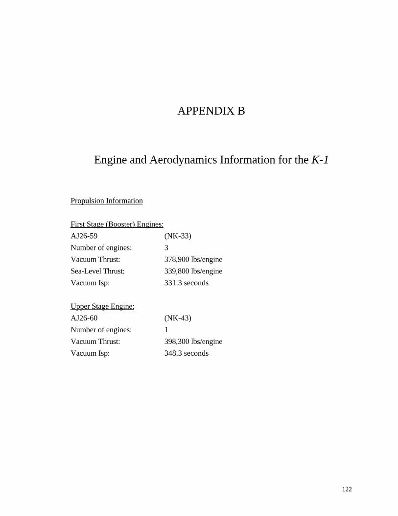
122
APPENDIX B
Engine and Aerodynamics Information for the K-1
Propulsion Information
First Stage (Booster) Engines:
AJ26-59 (NK-33)
Number of engines: 3
Vacuum Thrust: 378,900 lbs/engine
Sea-Level Thrust: 339,800 lbs/engine
Vacuum Isp: 331.3 seconds
Upper Stage Engine:
AJ26-60 (NK-43)
Number of engines: 1
Vacuum Thrust: 398,300 lbs/engine
Vacuum Isp: 348.3 seconds

123
Reference Aerodynamics Information:
Diameter (ft) Length (ft)
First (Booster) Stage: 22 60.2
Upper Stage: 13.2 61

124
APPENDIX C
Final Design Variables for K-1 Methods
Normalized*
Design
Variables
Manual
Iteration
FPI POBD 1 POBD 2 FOBD CO**
x[1] 1.00000 0.93887 0.92471 0.92518 0.95770 0.98153
x[2] 1.00000 1.03480 1.00458 1.00415 0.98194 1.00622
x[3] 1.00000 0.98765 0.99642 0.99606 1.01467 0.98931
x[4] 1.00000 0.98912 0.99324 0.99443 0.99879 0.96318
x[5] 1.00000 1.00587 1.00568 1.00484 1.01804 1.04452
x[6] 1.00000 0.95039 0.99606 0.99585 0.99162 0.93678
x[7] 1.00000 1.00017 1.00057 1.00070 0.99328 1.00460
x[8] 1.00000 0.99678 0.99877 0.99843 0.99264 0.99218
x[9] 1.00000 0.99761 0.99493 0.99404 0.99191 0.98777
x[10] 1.00000 1.00901 1.00836 1.00989 1.00376 1.00066
x[11] 1.00000 0.99541 0.99472 0.99401 0.99916 1.00348
x[12] 1.00000 0.99904 0.99721 0.99670 1.00185 0.99612
x[13]*** 1.00000 1.00429 1.01078 1.01078 1.01595 1.01122
x[14] 1.00000 1.00128 0.99917 0.99921 0.99721 0.99450
x[15] 1.00000 1.01851 0.98953 0.98940 0.99165 0.99284
x[16] 1.00000 1.04009 0.96236 0.96200 0.96753 0.96734
x[17] 1.00000 1.01842 0.99536 0.99527 0.99652 0.99644
x[18] 1.00000 1.00256 0.99174 0.99175 0.98816 0.98627
x[19] 1.00000 1.00715 0.99139 0.99136 0.99137 0.97831
x[20] N/A N/A 0.99139 0.99136 0.99137 N/A

125
x[21] N/A N/A N/A N/A 0.99648 N/A
x[22] N/A N/A N/A N/A 0.99714 N/A
x[23] N/A N/A N/A N/A 0.98665 N/A
x[24] N/A N/A N/A N/A 1.00018 N/A
x[25] N/A N/A N/A N/A 1.00023 N/A
x[26] N/A N/A N/A N/A 0.99993 N/A
* - The design variables are normalized with respect to the Manual Iteration Method results.
** - x[1] – x[19] are the local POST design variables and are listed here for comparison.
The system-level target design variables are listed in Chapter 7.
*** - x[13] is the objective function, payload weight.

126
APPENDIX D
RBCC Engine Inputs to SCCREAM for Stargazer
Engine Type: Ejector ScramJet
External Compression: Wedge with 1 Ramp
Rocket Primary Propellants: LOX/LH2
Number of Engines: 4
Force Accounting Method: Cowl-to-Tail
SLS Thrust (Ejector Mode Only): 20207.0 lbs per engine
Forebody and Inlet Characteristics
Inlet Area: 14.4 ft2 per engine
Aref for Ct Calculation: 14.4 ft2 per engine
Angle of Attack: 0.0 degrees
Cowl Height: 3.6 ft
Forebody Width: 16 ft
Centerline Distance from Nose to Cowl: 70.0 ft
Wedge Angle: 5.0 degrees
Rocket Primary Characteristics
Area Ratio: 18.0
Chamber Pressure: 1600.0 psi
Mixture Ratio: 8.0
Engine Station Efficiencies
Rocket Primary Combustor: 97.5 %
Rocket Primary Nozzle: 98.0 %
Combustor: 95.0 %

127
Nozzle: 98.0 %
Fuel Temperature: 500.0 R
Combustor Length
From Station 3 to 3': 2.0 ft
From Station 3' to 4: 3.0 ft
Subsonic Combustion
Geometry:
A* / A1 = 0.4
A1 / A3 = 1.8
A3' / A3 = 1.3
A4 / A3' = 1.2
Ae / A1 = 2.0
Ae' / A1 = 3.5
Fuel Injector Location & Start of Heat Release: 2.0 ft
End heat release: 5.0 ft
Fuel Injection Velocity: 3000.0 ft/s
Fuel Injection Angle: 0.0 degrees
Friction Coefficient: 0.001
Supersonic Combustion
Geometry:
A* / A1 = 0.4
A1 / A3 = 1.8
A3' / A3 = 1.2
A4 / A3' = 1.1
Ae / A1 = 3.5
Ae' / A1 = 3.5
Fuel Injector Location & Start of Heat Release: 1.0 ft
End heat release: 3.0 ft

128
Fuel Injection Velocity: 4000.0 ft/s
Fuel Injection Angle: 0.0 degrees
Friction Coefficient: 0.001
All-Rocket Mode
All-Rocket Mode Expansion Ratio: 180
All-Rocket Mode Mixture Ratio: 7.0

129
APPENDIX E
Stargazer Engine Multipliers & Scaling Equations
The inputs for the Stargazer engine deck are listed below with the equations used to
calculate each. Wg is the booster gross weight. All engine data is scaled by the original
Stargazer engine which was analyzed in SCCREAM and appears in Appendix D.
Ejector LOX flow rate = (((Wg*.7/4)/20207.4*83628.4)/420.429)*8/9;
Ejector linear thrust multiplier = 4*(.7*Wg/4)/20207.4;
Ramjet capture area = (57.6*.7*Wg/(20207.2*4));
Scramjet capture area = (57.6*.7*Wg/(20207.2*4));
All-Rocket LOX flow rate = (((Wg*.7/4)/20207.4*83628.4)/420.429)*7/8;
All-Rocket vacuum thrust = (Wg*.7/4)/20207.4*83628.4;
All-Rocket exit area = (Wg*.7/4)/20207.4*39.37464;
The inputs for the upper stage engine and the corresponding equations are as
follows, where USWg is the upper stage gross weight:
Upper stage vacuum thrust = USWg; (T/W of 1.0)
Upper stage exit area = 1.72/3350*USWg; (scaled by original engine)
The Isp 's for all engines are the same for iteration. For the booster’s ejector, ramjet,
and scramjet modes, the Isp’s are variable, depending on the Mach number, altitude, and

130
throttle. The Isp for all-rocket mode is 420.429 seconds. The upper stage engine Isp is 328
seconds.

131
APPENDIX F
Stargazer Weights Response Surfaces
The response surface equations for the Stargazer required weights inputs and
output are listed below. These equations were generated by JMP software [84]. Twenty-
seven responses were evaluated. The r-squared values are also listed for each equation.
In the equations below the following applies:
Mix = Booster Mixture Ratio,
MRus = Upper Stage Mass Ratio,
MRb = Booster Mass Ratio,
MRfb = Flyback Mass Ratio.
INPUTS:
Sref = 28669.806+3801.6667*Mix-33.83333*MRus-12037.25*MRb-30761.25*MRfb
+294.44445*Mix*Mix-10*MRus*Mix-3.5*MRus*MRus-1163.333*MRb*Mix
+33*MRb*MRus+1197.5*MRb*MRb1933.333*MRfb*Mix+30*MRfb*MRus
+7400*MRfb*MRb+7562.5*MRfb*MRfb;
RSquare = 0.996948
Wg = 5619835.2+580926.67*Mix-20480.33*MRus-2372700*MRb-5555900*MRfb
+34944.445*Mix*Mix-1066.667*MRus*Mix-747*MRus*MRus
-174960*MRb*Mix+8567*MRb*MRus+235119.5*MRb*MRb
-253500*MRfb*Mix+10335*MRfb*MRus+1319190*MRfb*MRb
+1226412.5*MRfb*MRfb;

132
RSquare = 0.993144
USWg = 1244.6944+246.11111*Mix+812.16667*MRus-586.4167*
MRb-1620.417*MRfb-16.66667*Mix*Mix+30*MRus*Mix
+64.5*MRus*MRus-23.33333*MRb*Mix-106*MRb*MRus
+81*MRb*MRb-133.3333*MRfb*Mix-255*MRfb*MRus
+320*MRfb*MRb+575*MRfb*MRfb;
RSquare = 0.999916
USSref = 44.572361+6.7583333*Mix+4.9258333*MRus-16.45875*MRb
-43.26875*MRfb-.361111*Mix*Mix+.2666667*MRus*Mix
+.0525*MRus*MRus-.633333*MRb*Mix-.9*MRb*MRus+1.705*MRb*MRb
-2.833333*MRfb*Mix-2.05*MRfb*MRus+6.825*MRfb*MRb
+11.5*MRfb*MRfb;
RSquare = 0.999389
OUTPUT:
Dry = 1186063.2+139966.47*Mix-3566.02*MRus-495759.8*MRb-1.2121e6*MRfb
+9580.2595 *Mix*Mix-343.4093*MRus*Mix-191.8127*MRus*MRus
-42297.67*MRb*Mix+1714.0259*MRb*MRus+49110.143*MRb*MRb
-65399.28*MRfb*Mix+2152.255*MRfb*MRus+286660.08*MRfb*MRb
+280425.16*MRfb*MRfb;
RSquare = 0.994115

133
APPENDIX G
Final Design Variables for Stargazer Methods
Normalized*
Design
Variables
Manual
Iteration
POBD CO**
x[1] 1.00000 1.01343 1.00950
x[2] 1.00000 0.72691 0.74060
x[3] 1.00000 1.34879 1.31626
x[4] 1.00000 0.65429 0.67414
x[5] 1.00000 0.95849 0.96799
x[6] 1.00000 1.00937 1.00937
x[7] 1.00000 0.97143 0.97211
x[8] 1.00000 0.92545 0.89952
x[9] 1.00000 1.00028 0.99722
x[10] 1.00000 1.03181 1.04580
x[11] 1.00000 1.00184 0.98929
x[12] 1.00000 1.04123 1.05636
x[13] 1.00000 1.42828 1.35862
x[14] 1.00000 1.41161 1.33825
x[15] 1.00000 1.59868 1.49127
x[16] 1.00000 1.75435 1.62455
x[17] 1.00000 1.31894 1.27074
x[18] 1.00000 1.00479 1.00612
x[19] 1.00000 1.06526 1.05827
x[20] 1.00000 0.76448 0.82243

134
x[21] 1.00000 0.66889 0.62573
x[22] 1.00000 0.91506 0.90209
x[23] 1.00000 1.00000 1.00001
x[24] 1.00000 1.00000 1.00000
x[25] 1.00000 1.00000 1.00000
x[26] 1.00000 1.25885 1.37569
x[27] 1.00000 0.75222 0.66925
x[28] 1.00000 0.97972 0.95254
x[29] 1.00000 1.00000 1.00000
x[30] 1.00000 1.00000 1.00000
x[31] 1.00000 1.00000 1.00000
x[32] 1.00000 1.05757 1.06434
x[33] 1.00000 1.02809 0.99030
x[34] 1.00000 0.81443 0.78530
x[35] 1.00000 0.74221 0.82734
x[36] N/A 1.00812 N/A
x[37] N/A 1.00210 N/A
x[38] N/A 0.99357 N/A
x[39] N/A 0.99177 N/A
*- The design variables are normalized with respect to the manual iteration method results.
** - x[1] – x[35] are the local POST design variables and are listed here for comparison.
The system-level target design variables are listed in Chapter 9.

135
REFERENCES
1. Miele, A. Flight Mechanics: Theory of Flight Paths. Reading, PA: Addison-Wesley,
1962.
2. Lawden, D. F. Optimal Trajectories for Space Navigation. London: Butterworths,
1963.
3. Vinh, Nguyen X. Optimal Trajectories in Atmospheric Flight. New York: Elsevier
Scientific Publishing Company, 1981.
4. Etkin, Bernard. Dynamics of Flight--Stability and Control. 2nd Edition. New York:
John Wiley & Sons, Inc., 1982.
5. Tartabini, P. V., R. D. Braun, and R. S. Chowdry. “A Comparison of Direct Trajectory
Optimization Techniques: Collocation vs. Numerical Integration.” AIAA Paper 95-
3481. August, 1995.
6. Betts, John T. “Survey of Numerical Methods for Trajectory Optimization.” Journal
of Guidance, Control, and Dynamics. Vol. 21, No. 2, pp. 193-207. March-April,
1998.
7. Troutman, John L. Variational Calculus and Optimal Control: Optimization with
Elementary Complexity. 2nd Ed. New York: Springer-Verlag New York, Inc., 1996.
8. Keller, Herbert B. Numerical Methods for Two-Point Boundary-Value Problems.
Massachussetts: Blaisdell, 1968.

136
9. Bailey, P. B., L. F. Shampine, and P. E. Waltman. Nonlinear Two Point Boundary
Value Problems. New York: Academic Press, 1968.
10. Martos, Bela. Nonlinear Programming Theory and Methods. New York: American
Elsevier Pub. Co., 1975.
11. Bazaraa, M. S., H. D. Sherali, and C. M. Shetty. Nonlinear Programming: Theory
and Algorithms. 2nd Ed. New York: Wiley, 1993.
12. Bryson, A. E. and Y. C. Ho. Applied Optimal Control: Optimization, Estimation, and
Control. Rev. USA: Hemisphere Publishing Corporation, 1975.
13. Leung, M. S. and A. J. Calise. “An Approach to Optimal Guidance of an Advanced
Launch Vehicle Concept.” Proceedings of the American Control Conference. pp.
1824-1828. 1990.
14. Speyer, Jason L. ‘Approximate Optimal Guidance for Aerospace Systems.’ AAS
Paper 94-070. February, 1994.
15. Park, S.-Y. “Launch Vehicle Trajectories with a Dynamic Pressure Constraint.”
Journal of Spacecraft and Rockets. Vol. 35, No. 6, pp. 765-773. November -
December, 1998.
16. Calise, A.J., N. Melamed, and S. Lee. “Design and Evaluation of a 3-D Optimal Ascent
Guidance Algorithm.” Journal of Guidance, Control, and Dynamics. Vol 21, No. 6,
pp 867-875. November-December, 1998.
17. Vlases, W. G., S. W. Paris, R. M. Lajoie, P. J. Martens, and C. R. Hargraves.
“Optimal Trajectories by Implicit Simulation, Version 3.0, User’s Manual.” WRDC-
TR-90-3506. Wright Patterson Air Force Base, OH. 1990.
18. Brauer, G. L., D. E. Cornick, and R. Stevenson. “Capabilities and Applications of the
Program to Optimize Simulated Trajectories.” NASA CR-2770. Feb. 1977.

137
19. Meder, D. S. and J. L. Searcy. “Generalized Trajectory Simulation (GTS), Volumes I-
V.” The Aerospace Corporation. SAMSO-TR-75-255. January, 1975.
20. Paris, S. “Overview of OTIS 3.0.” NASA Conference Publication No. 10187.
August, 1996.
21. Hallman, W. P. “Mission Timeline for a Shuttle-IUS Flight Using a Nonstandard
Shuttle Park Orbit.” TOR-0083 (3493-14)-1. The Aerospace Corporation. October,
1982.
22. Naftel, J. C. and R. W. Powell. “Flight Analysis for a Two-Stage Launch Vehicle with
a Glideback Booster.” Journal of Guidance, Control, and Dynamics. Vol. 8, No. 3,
pp. 340-343. May – June, 1985.
23. Lepsch, R. A. and J. C. Naftel. “Winged Booster Performance with Combined Rocket
and Airbreathing Propulsion.” Journal of Spacecraft and Rockets. Vol. 30, No. 6, pp.
641-646. November – December, 1993.
24. Anderson, R. L., J. T. Aguirre, S. A. Striepe, G. L. Brauer, and M. C. Engel. Program
to Optimize Simulated Trajectories (POST II): Guide for New Users. Preliminary,
Beta Release, Volume I. April, 1999.
25. Vanderplaats, Garret N. Numerical Optimization Techniques for Engineering Design:
with Applications. New York: McGraw-Hill Publishing Co. 1984.
26. Steward, D. V. Systems Analysis and Management: Structure, Strategy and Design.
New York: Petrocelli Books, Inc. 1981.
27. Sobieszczanski-Sobieski, J. “Multidisciplinary Design Optimization: An Emerging
New Engineering Discipline.” Presented at The World Congress on Optimal Design
of Structural Systems in Rio de Janeiro, Brazil. August, 1993.

138
28. Sobieszczanski-Sobieski, J. and R. T. Haftka. “Multidisciplinary Aerospace Design
Optimization: Survey of Recent Developments.” AIAA Paper 96-0711. January,
1995.
29. Rowell, L. F., R. D. Braun, J. R. Olds, and R. Unal. “Multidisciplinary Conceptual
Design Optimization of Space Transportation Systems.” Journal of Aircraft. Vol. 36,
No. 1, pp. 218-226. January-February, 1999.
30. Sobieszczanski-Sobieski, J. “Sensitivity Analysis and Multidisciplinary Optimization
for Aircraft Design: Recent Advances and Results.” Journal of Aircraft. December,
1990.
31. Celi, R. “Recent Applications of Design Optimization to Rotorcraft—A Survey.”
Journal of Aircraft. Vol. 36, No. 1, pp. 176-189. January-February, 1999.
32. Roy, Ranjit. A Primer on the Taguchi Method. New York: Van Nostrand Reinhold,
1990.
33. Phadke, Madhav. Quality Engineering Using Robust Design. New Jersey: Prentice-
Hall. 1989.
34. Olds, J. and G. Walberg. “Multidisciplinary Design of a Rocket-Based Combined-
Cycle SSTO Launch Vehicle Using Taguchi Methods.” AIAA Paper 93-1096.
February, 1993.
35. Olds, J. R. “Multidisciplinary Design Techniques Applied to Conceptual Aerospace
Vehicle Design.” Ph.D. Thesis. North Carolina State University. 1993.
36. DeLaurentis, D., P. S. Zink, D. Mavris, C. E. S. Cesnik, and D. P. Schrage. “New
Approaches to Multidisciplinary Synthesis: An Aero-Structures-Control Application
Using Statistical Techniques.” AIAA Paper 96-5501. October, 1996.
37. Zink, P. S., D. N. Mavris, D. M. Flick, and M. H. Love. “Impact of Active Aeroelastic
Wing Technology on Wing Geometry Using Response Surface Methodology.”

139
Presented at CEAS/AIAA/ICASE/NASA Langley International Forum on Aeroelasticity
and Structural Dynamics. June, 1999.
38. Mavris, D. N., D. A. DeLaurentis, O. Bandte, and M. A. Hale. “A Stochastic Approach
to Multidisciplinary Aircraft Analysis and Design.” AIAA Paper 98-0912. January,
1998.
39. Mavris, D. N., O. Bandte, and D. A. DeLaurentis. "Robust Design Simulation: A
Probabilistic Approach to Multidisciplinary Design." Journal of Aircraft . Vol. 36, No.
1, pp. 298-307. January-February, 1999.
40. Gage, P. J., R. D. Braun, and I. M. Kroo. “ Interplanetary Trajectory Optimization
Using a Genetic Algorithm.” Journal of Astronautical Sciences. Vol. 43, No. 1, pp.
59-76. January, 1995.
41. Way, D. and J. Olds. “Sirius: A New Launch Vehicle Option for Mega-Leo
Constellation Deployment.” AIAA Paper 97-3122. July, 1997.
42. Balling, R. J. and J. Sobieszczanski-Sobieski. “Optimization of Coupled Systems: A
Critical Overview of Approaches.” AIAA Paper 94-4330. September, 1994.
43. Sobieszczanski-Sobieski, J. “Optimization by Decomposition: A Step from Hierarchic
to Non-Hierarchic Systems.” NASA CP-3031. September, 1989.
44. Altus, S., and I. M. Kroo. “Concurrent Wing Design and Flight-Path Optimization
Using Optimizer-Based Decomposition.” AIAA Paper 98-4920. September, 1998.
45. Altus, S. S. “Multidisciplinary Aircraft Design Optimization Using Single-Level
Decomposition.” Ph.D. Thesis. Stanford University. August, 1997.
46. Braun, R. D., R. W. Powell, R. A. Lepsch, D. O. Stanley, and I. M. Kroo.
“Comparison of Two Multidisciplinary Optimization Strategies for Launch-Vehicle
Design.” Journal of Spacecraft and Rockets. Vol. 32, No.3, pp. 404-410. May-June,
1995.

140
47. Kroo, I., S. Altus, R. Braun, P. Gage, and I. Sobieski. “Multidisciplinary Optimization
Methods for Aircraft Preliminary Design.” AIAA Paper 94-4325. September, 1994.
48. Jacobsmeyer, H. A. and R. J. Balling. “When Can Multi-Level Optimization Reduce
Computational Effort?” AIAA Paper 98-4921. September, 1998.
49. Balling, R. J. and C. A. Wilkinson. “Execution of Multidisciplinary Design
Optimization Approaches on Common Test Problems.” AIAA Journal. Vol. 35, No. 1,
pp. 178-186. January, 1997.
50. Braun, R. D. “Collaborative Optimization: An Architecture for Large-Scale
Distributed Design.” Ph.D. Thesis. Stanford University. May, 1996.
51. Braun, R. D., R. W. Powell, R. A. Lepsch, D. O. Stanley, and I. M. Kroo.
“Multidisciplinary Optimization Strategies for Launch Vehicle Design.” AIAA Paper
94-4341. September, 1994.
52. Braun, R. D., A. A. Moore, and I. M. Kroo. “Collaborative Approach to Launch
Vehicle Design.” Journal of Spacecraft and Rockets. Vol. 34, No. 4, pp. 478-486.
July-August, 1997.
53. Sobieski, I. and I. Kroo. “Collaborative Optimization Applied to an Aircraft Design
Problem.” AIAA Paper 96-0715. January, 1996.
54. Braun, R. D. and I. Kroo. “Development and Application of the Collaborative
Optimization Architecture in a Multidisciplinary Design Environment.”
Multidisciplinary Design Optimization: State of the Art.. Philadelphia, PA: SIAM
Publications. 1997.
55. Rawlings, M. R. and R. J. Balling. “Collaborative Optimization with Disciplinary
Conceptual Design.” AIAA Paper 98-4919. September, 1998.

141
56. Budianto, I. A. and J. R. Olds. “A Collaborative Optimization Approach to Design and
Deployment of a Space Based Infrared System Constellation.” 2000 IEEE Aerospace
Conference Proceedings. Paper 13.0203. Big Sky, Montana. March, 2000.
57. Sobieski, I. P. “Multidisciplinary Design Using Collaborative Optimization.” Ph.D.
Thesis. Stanford University. August, 1998.
58. Manning, V. Large-Scale Design of Supersonic Aircraft Via Collaborative
Optimization.” Ph.D. Thesis. Stanford University. June, 1999.
59. Balling, R. J. and J. Sobieszczanski-Sobieski. “An Algorithm for Solving the System-
Level Problem in Multilevel Optimization.” AIAA Paper 94-4333. September, 1994.
60. Sobieszczanski-Sobieski, J., B. James, and M. Riley. “Structural Design by
Generalized, Multilevel Decomposition.” AIAA Journal. Vol. 25, No. 1, pp. 139-145.
January, 1987.
61. Walsh, J. L., K. C. Young, J. I. Pritchard, H. M. Adelman, and W. R. Mantay.
“Integrated Aerodynamic/Dynamic/Structural Optimization of Helicopter Rotor Blades
Using Multilevel Decomposition.” NASA TP-3465, January, 1995.
62. Beltracchi, T. J. “Decomposition Approach to Solving the All-Up Trajectory
Optimization Problem.” Journal of Guidance, Control, and Navigation. Vol. 15, No.
3, pp. 707-716. May-June, 1992.
63. Cramer, E. J., J. E. Dennis, Jr., P. D. Frank, R. M. Lewis, and G. R. Shubin. “Problem
Formulation for Multidisciplinary Optimization.” SIAM Journal of Optimization. Vol.
4, No. 4, pp. 754-776. November, 1994.
64. Sobieszczanski-Sobiesk, J., J.-F. Barthelemy, and K. M. Riley. “Sensitivity of
Optimum Solutions to Problem Parameters.” AIAA Journal. Vol. 20, pp. 1291-1299.
September, 1982.

142
65. Braun, R. D., I. M. Kroo, and P. J. Gage. “Post-Optimality Analysis in Aerospace
Vehicle Design.” AIAA Paper 93-3932. August, 1993.
66. Kodiyalam, S. “Evaluation of Methods for Multidisciplinary Design Optimization
(MDO), Phase 1.” NASA CR-1998-208716. September, 1998.
67. Alexandrov, N. M. and S. Kodiyalam. “ Initial Results of an MDO Method Evaluation
Study.” AIAA Paper 98-4884. September, 1998.
68. Zang, T. A. and L. L. Green “ Multidisciplinary Design Optimization Techniques:
Implications and Opportunities for Fluid Dynamics Research.” AIAA Paper 99-3798.
June-July, 1999.
69. Korte, J. J., R. P. Weston, and T. A. Zang. “Multidisciplinary Optimization Methods
for Preliminary Design.” AGARD Interpanel Symposium “Future Aerospace
Technology in the Service of the Alliance.” Paris, France. April, 1997.
70. Kohrs, R. and R. Petersen. “Development of the K-1 Two-Stage, Fully-Reusable
Launch Vehicle.” AIAA Paper 98-1540. April, 1998.
71. J. Andrews. “Status of the Kistler Reusable Launch Vehicle.” AIAA Paper 98-3955.
July, 1998.
72. Kistler Aerospace web site: http://www.kistleraerospace.com.
73. Anisimov, V. S., T. C. Lacefield, and J. Andrews. “Evolution of the NK-33 and NK-43
LOX/Kerosene Engines.” AIAA Paper 97-2680. July, 1997.
74. Mecham, M. “Aerojet Acquires Major K-1 Engine Shipment.” Aviation Week and
Space Technology. Vol. 147, No. 10, pp. 61-62. September, 1997.
75. Kohrs, R. Personal Communications. June, 1999 and November, 1999.

143
76. Sova, G. and P. Divan. “Aerodynamic Preliminary Analysis System II, Part II –
User’s Manual.” NASA CR-182077. April, 1991.
77. DOT™ User’s Manual, Version 4.20. Vanderplaats Research & Development, Inc.
Colorado: 1995.
78. Olds, J.R., L. Ledsinger, J. Bradford, A. Charania, D. McCormick, and D. R. Komar.
“ Stargazer: A TSTO Bantam-X Vehicle Concept Utilizing Rocket-Based Combined
Cycle Propulsion.” AIAA Paper 99-4888. November, 1999.
79. Bradford, J. E. and J. R. Olds. “SCCREAM v. 5: A Web-Based Airbreathing
Propulsion Analysis Tool.” AIAA Paper 99-2104. June, 1999.
80. Ryan, Richard M., W. J. Rothschild, and D. L Christensen. “Booster Main Engine
Selection Criteria for the Liquid Fly-Back Booster.” JANNAF JPM. July, 1998.
81. Rothschild, W. and E. Schuster. “Airbreathing Propulsion System Design Concepts
for a Reusable First Stage Rocket Booster.” AIAA Paper 99-2380. July, 1999.
82. Anonymous. Lockheed Martin literature.
83. Budianto, I. A., J. R. Olds, and N. C. Baker. “Demonstration of CLIPS as an
Intelligent Front-End for POST.” AIAA Paper 99-0110. January, 1999.
84. Anonymous. JMP Version 3.1. SAS Institute, Inc.: Cary, NC, 1995.

144
VITA
Laura Anne Ledsinger was born on May 26, 1972 in Baltimore, Maryland. After
many years of preparatory education, she graduated as valedictorian from Patapsco High
School in 1990. In September of that year, she joined the Georgia Institute of Technology
for her undergraduate studies in Aerospace Engineering. She received her Bachelor of
Science degree, with Highest Honor, in June of 1994. Laura was a recipient of the Donald
Dutton Outstanding Aerospace Senior Award in 1994.
That September, she continued her studies at Georgia Tech, this time, as a graduate
student. Laura received her Master of Science degree in Aerospace Engineering in March
of 1996 while working for Dr. C.-H. Chuang. For that degree, her research was in the area
of the second variation in optimal guidance and control.
In January of 1997, Laura joined Dr. John R. Olds who supervised her doctoral
research. The culmination of her doctoral research is the thesis entitled, “Solutions to
Decomposed Branching Trajectories with Powered Flyback Using Multidisciplinary
Design Optimization.” In addition to her thesis work, she was the performance/trajectory
analyst on many team design projects including Hyperion, Space Solar Power (ETO),
Stargazer, and Starsaber. Laura was the project lead and trajectory analyst for the
Stargazer/Starsaber designs from June, 1998 through December, 1999. Beginning in
January, 2000, Laura took a less involved role in the Starsaber designs, as operations and
economics analyst, in order to concentrate on this thesis. In the summer of 1998, she
carried out work on the Stargazer design, among others, at NASA Marshall Space Flight
Center in Huntsville, AL. Another interesting note is that Laura was a member of the design
team that won the X-Prize® University Design Competition in May of 1998. Laura is a
member of the American Institute of Aeronautics and Astronautics.