RESEARCH Revista Mexicana de Fısica66 (5) 643–655 SEPTEMBER-OCTOBER 2020

Solutions ofq-deformed multiple-trapping model for charge carrier transportfrom time-of-flight transient photo-current in amorphous semiconductors

F. Serdouka, A. Boumalia, A. Makhloufa,b, and M. L. BenkhediraaLaboratoire de Physique Appliquee et Theorique, LPAT,

Universite Larbi-Tebessi, Tebessa, Algeria.bUniversite de Haute Alsace, IRIMAS-Departement de Mathematiques,

68093 Mulhouse, France.e-mail: fadila.serdouk@univ-tebessa.dz; abdelmalek.boumali@univ-tebess.dz;

boumali.abdelmalek@gmail.com; abdenacer.makhlouf@uha.fr; benkhedir@gmail.com

Received 5 February 2020; accepted 22 May 2020

The aim of this paper is to investigate the description of theq-deformed multiple-trapping equation for charge carrier transport in amorphoussemiconductors. We first modify the multiple-trapping model of charge carriers in amorphous semiconductors from time-of-flight transientphoto-current in the framework of theq-derivative formalism, and then we construct our simulated current by using an approach basedon the Laplace method. It is implemented in a program proposed recently by [14] which allows us to construct a current using the Padeapproximation expansion. Furthermore, we study the influence of the parameterq of theq-calculus formalism on the drift mobility.

Keywords: Amorphous semiconductors; multiple-trapping model; drift mobility; Laplace technics; time-of-flight;q−deformed formalism.

PACS: 72.80.Ng; 72.40.+w; 73.61.Jc DOI: https://doi.org/10.31349/RevMexFis.66.643

1. Introduction

Quantum groups and quantum algebras have attracted muchattention of physicists and mathematicians recently. Therehad been a great deal of interest in this field, especially af-ter the introduction of theq-deformed harmonic oscillator.Quantum groups and quantum algebras have found unex-pected applications in theoretical physics [1]. From the math-ematical point of view they areq−deformations of universalenveloping algebras of the corresponding Lie algebras, beingalso concrete examples of Hopf algebras. When the deforma-tion parameterq is set equal to 1, we recover usual Lie alge-bras. The realization of the quantum algebra SU(2) in termsof the q-analogue of the quantum harmonic oscillator [2, 3]has initiated much work on this topic [4–6]. Biedenharn andMacfarlane [2, 3] have studied theq-deformed harmonic os-cillator based on an algebra ofq-deformed creation and anni-hilation operators. They have found the spectrum and eigen-values of such a harmonic oscillator under the assumptionthat there is a state with a lowest energy eigenvalue.

In the last few years,q−deformations have become atopic of great interest and various applications have beenfound in several branches of physics, such asq−deformationof the harmonic oscillator,q−deformed Morse oscilla-tor, classical and quantumq−deformed physical systems,Jaynes-Cummings model and the deformed-oscillator alge-bra, q−deformed supersymmetric quantum mechanics, forsome modifiedq-deformed potentials, on the thermostatis-tic properties of aq-deformed ideal Fermi gas,q−deformedTamm-Dancoff oscillators,q-deformed fermionic oscillatoralgebra, and thermodynamics, and finally on the fermionicq−deformation and its connection to thermal effective massof a quasiparticle (see Ref. [7] and references therein).

The displacement of charge through a dielectric mate-rial plays an essential role in a wide variety of electronics orimaging devices. A detailed understanding on the process dy-namics can provide considerable information concerning thematerial’s electronic structure. Experimentally, the time rateof displacement of charge, as well as the efficiency of theirgeneration by light or energetic electrons, has been studiedusing a time-of-flight technique (for more detail about thistechnique see Refs. [8-11]).

In TOF measurements, a semiconductor thin film is sand-wiched between electrodes and at least one of the electrodesis blocking for carrier injection, and through one of the elec-trodes a short light pulse of strongly absorbed light excites athin layer of electron-hole pairs. Depending on the polarityof an applied electric field, either holes or electrons are drawninto the bulk. The carriers reach the opposite electrode in atransit timetr, which is easily identified as either a rapid dropin the transient photo-current in case of nondispersive trans-port or an inflection point in the double logarithmic plot ofthe transient photo-current in case of dispersive transport. Inaddition, a dispersive transport is the result of a broad distri-bution of release times from localized states. This distribu-tion can arise from a sped of binding energies of traps (MT)or from a distribution of hopping rates among iso-energeticlocalized states. If it arises from hopping, dispersion occursonly in the presence of an electric field. This is because, aspointed out by Schmidlin and Kastner [8, 9], the occupationof the various states cannot change with time in the absenceof the field since they are already in thermal equilibrium.When the field is turned on, the states are no longer in equi-librium because their energies are altered, and the dispersionbegins. For these reasons, the (TOF) measurement method isa useful technique to evaluate transit time for mobile objects

644 F. SERDOUK, A. BOUMALI, A. MAKHLOUF, AND M. L. BENKHEDIR

and is often used for investigating the charge carrier transportproperties in various condensed materials including inorganicand organic semiconductors. The resulting transient currentprovides us with not only transit time but also information ondynamical events in charge transport through a sample, suchas trapping and releasing of carriers in trap states, carrier dif-fusion, and percolation.

Schmidlin and Noolandi [10, 11] proposed the multiple-trapping model (MTM) to describe such dynamic events ofcharge carriers in a sample with conventional sets of coupledkinetic equations for trapping and thermally releasing rates.This method can reproduce the experimental current signalI (t), if a subset of trapping- and releasing-rate parametersare suitably assumed. Thus, the MTM has been widely andsuccessfully used to analyze transient-current decays not onlyin inorganic but also in various organic semiconductors. Thefilms include amorphous inorganic or organic semiconduc-tors, with adequate supposition of trapping and releasing pa-rameters in the form of continuous distribution of trap statessuch as an exponential distributione−E/kBT , a Gaussian dis-tribution or other shapes of trap distribution. However, thismethod is applicable only when a shape of the trap distribu-tion is appropriately taken to describe the distribution of lo-calized states playing the major role in trapping events [12].

Naito et al., [13–16] have proposed a spectroscopicmethod for extracting localized-state distributions from ananalysis of transient photo-current measured with transientphoto-conductivity or the TOF technique using the Laplacetransform, within a multiple-trapping framework and bymeans of appropriate approximations. Using a method basedon the Laplace transform method, has a number of advan-tages when compared with other methods: (i) the localized-state distributions in materials exhibiting either nondispersiveor dispersive transport are extracted, the analysis is compu-tationally straightforward and rapid, and (ii) the localized-state distributions are extracted from both pre- and post-monomolecular recombination regimes of transient photo-conductivity or from both pre- and post-transit time regimesof TOF photo-current transient, which hence leads to themeasurement of a wider range of localized-state distributions.

After all this brief description, we are ready to expose theobjectives of our paper: encouraged by the fact that theq-deformed formalism has interesting and promising results inphysics (see [17] and references therein), we are in measureto do the following tasks (i) rewriting the (MTM) equationsin the framework of theq-deformed formalism, and (ii) thenconstruct theoretically the deformed simulated currents: thisconstruction is given by using a program based on the Padeapproximation. This program allows us to obtain these cur-rents [18]. In all calculations, the electric field has the fol-lowing form [19,20]

ξ (x) = k1 − k2x. (1)

So far, the MTM equations with this type of the electric fieldhave not been studied in the literature. From Eq. (1), we no-tice the following: (i)ξ (x) = −dV /dx can also be consid-

ered as an external force associated with the potentialV (x),(ii) k2 = 0 corresponds to the important case of external con-stant force, and (iii) finallyk1 = 0, corresponds to the so-called Uhlenbeck-Ornstein process. The Uhlenbeck-Ornsteinprocess describes the stochastic evolution of particles underthe influence of friction. This process is stationary, Gaussian,and Markov, which makes it a good candidate to representstationary random noise [19,20].

Thus, in order to realize the goals of this paper, we firststudy the usual case,i.e., without introducing any deforma-tion. Then, we consider and discuss the problem in the frame-work of q-calculus.

This paper is organized as follows: after an introduction,we treat analytically the TOF measurements with the mul-tiple trapping model (MTM) in Sec. 2. Then, in Sec. 3 weextend and study the (MTM) in the framework ofq-calculusformalism. The paper is ended by a conclusion provided inSec. 4.

2. Analytical treatment of the tof measure-ments with the multiple trapping model(MTM)

2.1. Solutions of (MTM) equations via the Laplacetransform (LT)

The continuity equations which define the multiple-trappingproblem are first formulated in the familiar context of an elec-tronic carrier moving through extended states with localizedgap states acting as trays. It is then shown that the same equa-tions apply to any mobile entity which simply stops and startsat random from a distribution of resting places. The proba-bility of generation per unit volume per unit time is denotedgν (x, t) = p0δ (t) δ (x). Subsequent to generation, the holedrifts (under the influence of anx-directed electrostatic forceeF , wheree is the fundamental electronic charge) toward asubstrate atx = L. At a point x, where the hole may becaptured and released from a trap, the appropriate continuityequations may be written [9–11]

∂p (x, t)∂t

= −m∑

i

∂pi (x, t)∂t

+ p0δ (t) δ (x)− ∂fp

∂x, (2)

∂pi (x, t)∂t

= ωip (x, t)− γipi (x, t) , (3)

wherex is the distance from the illuminated surface,p(x, t)andpi(x, t) are the local populations of the transport statesand trapi, andp0 is the injected free carrier density per theunit area. The delta functions define the initial condition for(TOF) experiment. The local flux of mobile holes may bewritten

fp = ξ (x) p (x, t) , (4)

Rev. Mex. Fıs. 66 (5) 643–655

SOLUTIONS OFQ-DEFORMED MULTIPLE-TRAPPING MODEL FOR CHARGE CARRIER TRANSPORT FROM TIME-OF-FLIGHT . . . 645

whereξ (x) is the electric field. The simplest form that canbe given for this function is

ξ (x) = k1 − k2x, (k2 ≥ 0) . (5)

Now, using Eqs. (4) and (5), we obtain

∂p (x, t)∂t

= −m∑

i

∂pi (x, t)∂t

+ k2p

− (k1 − k2x)∂p (x, t)

∂x+ p0δ (t) δ (x) , (6)

∂pi (x, t)∂t

= ωip (x, t)− γipi (x, t) . (7)

The delta function in Eq. (6) defines the optical excitation forthe TOF experiment. These equations can be solved usingLaplace transforms under the initial and boundary conditionsof p(x, 0) = 0 andp(0, t) = 0.

The Laplace transform ofp(x, t) is defined as

p(x, s) =

∞∫

0

p (x, t) e−stdt. (8)

Using this definition, we obtain

(k1 − k2x)∂p(x, s)

∂x+ a′ (s) p(x, s) = p0δ (x) (9)

with

a′ (s) = s +m∑

i

sωi

s + γi− k2

= s + s

Ef∫

0

σνg (E)

s + νe−E

kBT

dE

︸ ︷︷ ︸a(s)

−k2. (10)

Now, the general solutions of (9) are

p(x, s) = p0

(1− k2k1

x)a(s)k2

k1 − k2x. (11)

For a TOF experiment, the photo-current is given by [9–11]

I(t) =e

L

L∫

0

(k1 − k2x) p (x, t) dx, (12)

whiche is the charge of a carrier: this equation is transformedinto

I (s) =e

L

L∫

0

(k1 − k2x) p (x, s) dx

=ep0

L

L∫

0

(1− k2

k1x)

a(s)k2 dx

=ep0k1

L

{1−

(1− k2

k1L

) a(s)k2

+1}

a(s) + k2, (13)

with k1 = µ0F , 0 < k2 < k1/L = µ0F/L, andt0 = L/k1

is the transit time of untrapped carrier. With the followingsubstitutionsα = k2L/k1 < 1, Eq. (13) is rewritten, withthe new parameterα, as follows

I (s) =ep0k1

L

{1− (1− α)

a(s)t0αk1

+1

}

a(s) + αt0

, (14)

where the parameterα contains the influence of both param-etersk1 andk2.

In the limit case, wherek2 → 0 (case of external constantforce), and by using thatax = exlna, we have

(1− k2

k1x

) a(s)k2

= ea(s)k2

ln(1− k2

k1x)' e−

a(s)xk1 = e−

a(s)t0xL

(1− k2L

k1

) a(s)k2

+1

= e

(1+

a(s)k2

)ln

(1− k2L

k1

)

≈ e−k2Lk1 e−

a(s)k1

L = e−a(s)t0 , (15)

and consequently, both (11) and (14) become

p (x, s) =p0

k1e−

a(s)t0L x, (16)

I (s) =ep0

t0a (s)

(1− e−a(s)t0

). (17)

Therefore, we recover the usual form of charges and cur-rents [10,11].

2.2. Results and discussion

In order to construct a current numerically, we proceededwith the following steps: as well-known, the inverse Laplaceof a function is given by

I (t) =1

2πi

c+i∞∫

c−i∞

I (s) estdt, (18)

which I (s) is defined by Eq. (13). When we use the follow-ing change of variables,z = st, anddz = sdt, the integralbecomes

I (t) =1

2πit

c′+i∞∫

c′−i∞

I(z

t

)ezdz. (19)

To calculate the last integral we use the method exposedin [18]. So, according to Eq. (19), the computed current canbe obtained as follows: (i) Firstly, we express the function

Rev. Mex. Fıs. 66 (5) 643–655

646 F. SERDOUK, A. BOUMALI, A. MAKHLOUF, AND M. L. BENKHEDIR

ez in its Pade approximation expansion: Pade approxima-tion of a function is somewhat similar to a Taylor series, ex-cept that the expansion is a ratio of two polynomials. (ii)Secondly, we apply the Residue theorem to obtain the de-sirable function,i.e., the computed currentI(t). Thus, inour case, we calculated the inverse Laplace transform nu-merically, using the Pade approximation (a rational approxi-mation with polynomials of 8-degree). The physical quan-

tities used in the computation wereσνth = 10−7 cm3/s,ν = 1012 s−1, T = 300 K, and g (E) = 1021e−(E/kbT0)

with kb = 8.625× 10−5 eVK−1 is the Boltzmann constant.Now, we are ready to show and discuss all the results

found by the program used to obtain our simulated currents.Figure 1 shows the normalized photo-currents vs times in

the (log-log) scale for different values of parametersk1 andk2 or α = k2L/k1.

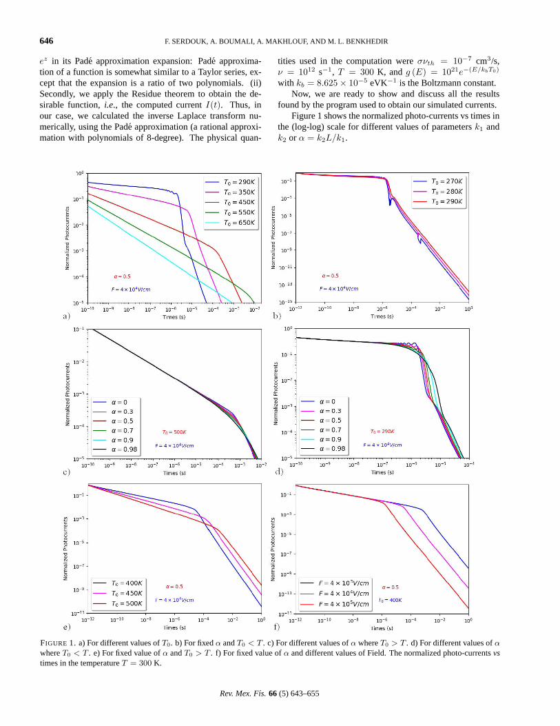
FIGURE 1. a) For different values ofT0. b) For fixedα andT0 < T . c) For different values ofα whereT0 > T . d) For different values ofαwhereT0 < T . e) For fixed value ofα andT0 > T . f) For fixed value ofα and different values of Field. The normalized photo-currentsvstimes in the temperatureT = 300 K.

Rev. Mex. Fıs. 66 (5) 643–655

SOLUTIONS OFQ-DEFORMED MULTIPLE-TRAPPING MODEL FOR CHARGE CARRIER TRANSPORT FROM TIME-OF-FLIGHT . . . 647

In Fig. 1a), we present the normalized currents for fixedvalueα = 0.5 and for various characteristic temperaturesT0.It is clearly seen that the transient photo-current decreaseswith time. For non-dispersive transport, withT0 = 250 K,the transit time can be obtained at the intersection of the tran-sient photo-current with the time-axis. Similar results are ob-tained for dispersive transient photo-current. Now, for all thetemperaturesT0 < 300 K, as shown in Fig. 1b), we observethat all the curves have typically the same behavior in pre-and post-transient regime.

Figures 1c) and 1d) depict the behavior of the currentsin both T < T0 andT > T0 interval of temperatures, andthat for various values ofα: in this case, we specified tworegimes: in the region whereT0 > T , all the curves in bothpre- and post transient regime are the same. In the other hand,whereT0 < T , these curves show that the form of the cur-rents in the pre-transient regime are identical contrarily to thecase of the post-regime where the difference becomes clear.

Figures 1e) and 1f) illustrate the current transients at vari-ous values of applied electric fields for a fixed value of the pa-rameterα. An interesting observation pointed out in Fig. 1f)is that the inflection point is affected by the applied field. Thetransit time is much shorter than the mono-molecular recom-bination lifetime. In this case, the inflection points shift to-ward a shorter time regime by increasing the applied electricfield. This means that the inflection point is due to the transittime. From these results, we can experimentally distinguishwhether or not the inflection point is the charge carrier transittime: if the inflection point becomes shorter with an appliedelectric field, then the inflection point is charge carrier transittime.

3. Solutions of a multiple-trapping equationsin the framework of q-deformed formalism

We aim in this section to discuss in the frame work ofq-calculus the problem described by continuity equationsEqs. (2) and (3). We present in the Appendix A a surveyof q-calculus algebraic properties.

3.1. q-derivative and q-integral

Theq-derivative, in the framework of theq-calculus formal-ism, is defined as

Dqf (x) ≡ limx→y

f (x)− f (1y)xªq y

= {1 + (1− q) q} df (x)dx

. (20)

The development of this framework ofq-deformations in-spired the definition of deformed expressions for the loga-rithm and exponential functions, namely, theq-logarithm andtheq-exponential (q-exponential Tsallis [19]), first proposed

as

lnq x =x1−q − 1

1− q, x > 0, (21)

eq (x) = {1 + (1− q)x}1

1−q

+ , (x, q) ∈ R (22)

where[A]+ ≡ max {A; 0} (1 + (1− q)x > 0). Both equa-tions can be rewritten as

lnq x =

{x1−q−1

1−q q 6= 1, x > 0ln x q = 1,

(23)

eq (x) =

{{1 + (1− q)x} 1

1−q q 6= 1, (x, q) ∈ R,

e (x) q = 1,(24)

where both equations are restricted to the following condition1 + (1− q)x 6= 0. Also, we have the following well-knownrelations:

lnq (xy) = lnq x + lnq y + (1− q) lnq x lnq y, (25)

eq (x) eq (y) = eq (x + y + (1− q)xy)

≡ eq (x⊕ y) , (26)

where (see Appendix A)

x⊕ y = x + y + (1− q)xy. (27)

Theq-derivative obeys

• Leibniz rule

Dq {f (x) g (x)} = Dq {f (x)} g (x)

+ f (x)Dq {g (x)} , (28)

• the chain rule

Dq {f (g (x))} =df

dgDq {g} . (29)

The correspondingq-integral is given by∫

q

f (x) dqx =∫

f (x)1 + (1− q)x

dx, (30)

with

dqx = limx→y

xªq y =1

1 + (1− q)xdx. (31)

3.2. Solutions

Now, when introducing theq-derivative formula, Eqs. (2)and (3) become

∂p (x, t)∂t

=−m∑

i

∂pi (x, t)∂t

+p0δ (t) δ (x)−Dqfp, (32)

∂pi (x, t)∂t

= ωip (x, t)− γipi (x, t) , (33)

Rev. Mex. Fıs. 66 (5) 643–655

648 F. SERDOUK, A. BOUMALI, A. MAKHLOUF, AND M. L. BENKHEDIR

with

Dqf (x) = {1 + (1− q)x} df (x)dx

, (34)

and here

fp (x) = (k1 − k2x) p (x, t) . (35)

Using Eqs. (34) and (35), Eq. (32) is transformed into

∂p (x, t)∂t

= −m∑

i

∂pi (x, t)∂t

− {1 + (1− q)x}

×(−k2p (x, t) + (k1 − k2x)

∂p (x, t)∂x

)

+ p0δ (t) δ (x) . (36)

By using the Laplace transform method, Eq. (36) reads as

{1 + (1− q)x} (k1 − k2x)∂p(x, s)

∂x− {a (s)

− k2 {1 + (1− q) x}}p (x, t) = p0δ (x) . (37)

The solutions of Eq. (37) are

p(x, s) =p0k

− a(s)k2+(1−q)k1

1 exp(

a(s) lnk1−k2x

1+(1−q)x

k2+(1−q)k1

)

k1 − k2x. (38)

In the limit case, whereq →, 1, we recover the Eq. (16).The q-deformed Laplace of current has the following

form

Iq (s) =e

L

L∫

0

(k1 − k2x) p (x, s) dqx

=e

L

L∫

0

(k1 − k2x) p (x, s)1 + (1− q)x

dx. (39)

Putting Eq. (38) into Eq. (39) leads to

Iq (s) =ep0

L

×L∫

0

k− a(s)

k2+(1−q)k11 exp

(a(s) ln

k1−k2x

1+(1−q)x

k2+(1−q)k1

)

(1 + (1− q) x)dx. (40)

The general solution of this integral is

Iq (s) = Aq (s) [Bq (s) 2F1 (a1, b1, c1, d1)

+ Cq (s) 2F1 (a1, b1, c1, d2)], (41)

where

Aq (s) =−ep0k

− a(s)k2+(1−q)k1

1

La (s)

×(

(1 + (1− q) L) (1− q)2

(k2 + (1− q) k1)2

)− k1+k2+a(s)k2+(1−q)k1

, (42)

Bq (s) = −(

1− q

k2 + (1− q) k1

) k1q

k2+(1−q)k1

×(

(1 + (1− q)L) (1− q)k2 + (1− q) k1

)− k1+k2+a(s)k2+(1−q)k1

, (43)

Cq (s) = (−1 + (−1 + q) L)(

1− q

k2 + (1− q) k1

) k1+k2+a(s)k2+(1−q)k1

×(

(1 + (1− q)L) (1− q)k2 + (1− q) k1

) k1q

k2+(1−q)k1

, (44)

with

a1 = b1 = − a (s)k2 + (1− q) k1

, (45)

c1 = 1− a (s)k2 + (1− q) k1

, d1 =k2

k2 + (1− q) k1,

d2 =k2 (1 + (1− q) L)k2 + (1− q) k1

, (46)

and2F1 is the hypergeometric function.In this stage, an important remark can be made: following

these equations, we observe that obtaining the exact form ofcurrents is a very hard task. To overcome this problem, seek-ing simplicity, we will concentrate only on the case wherek2 = 0 (constant electric field). So, the form of the currentsI (s) as well as the chargesp (x, s) reduced to the followingrelations:

I (s) =ep0k1

La (s)

(1− eq (L)−

a(s)k1

), (47)

p (x, s) =p0

k1eq (x)−

a(s)k1 , (48)

with

eq (L) = {1 + (1− q)L} 11−q . (49)

In the limit case, whereeq (x)q→1 = exp (x), we recoverthe desired relations of currents and charges as described byEqs. (16) and (17).

Now, before commenting on our results, we can note thatthe linear form of the electric field can be considered as adeformation whose parameter isk2/k1. Starting with the fol-lowing equation

p(x, s) =p0

k1 − k2x

(1− k2

k1x

) a(s)k2

. (50)

Rev. Mex. Fıs. 66 (5) 643–655

SOLUTIONS OFQ-DEFORMED MULTIPLE-TRAPPING MODEL FOR CHARGE CARRIER TRANSPORT FROM TIME-OF-FLIGHT . . . 649

Setting−(k2/k1) = 1 − q or q = 1 + (k2/k1), Eq. (50) istransformed into

pq(x, s) =p0

k1 − k2x

[(1 + (1− q)x)

11−q

]− a(s)

k1 ,

=p0

k1

(1

1+ (1−q)x

) [(1+ (1−q)x)

11−q

]− a(s)

L t0 ,

=p0

k1

(1

1 + (1− q)x

)eq (x)−

a(s)L t0 . (51)

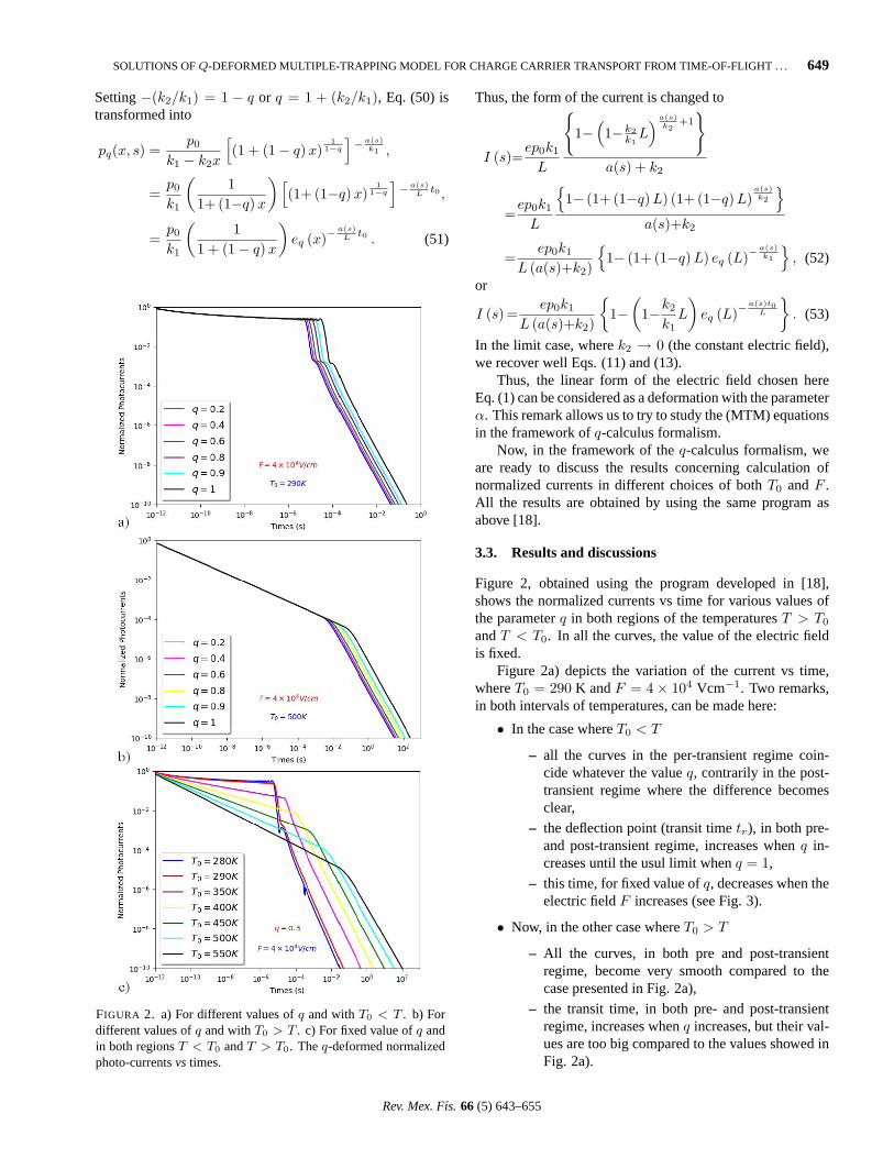
FIGURA 2. a) For different values ofq and withT0 < T . b) Fordifferent values ofq and withT0 > T . c) For fixed value ofq andin both regionsT < T0 andT > T0. Theq-deformed normalizedphoto-currentsvs times.

Thus, the form of the current is changed to

I (s)=ep0k1

L

{1−

(1−k2

k1L

) a(s)k2

+1}

a(s) + k2

=ep0k1

L

{1− (1+ (1−q)L) (1+ (1−q) L)

a(s)k2

}

a(s)+k2

=ep0k1

L (a(s)+k2)

{1− (1+ (1−q)L) eq (L)−

a(s)k1

}, (52)

or

I (s)=ep0k1

L (a(s)+k2)

{1−

(1−k2

k1L

)eq (L)−

a(s)t0L

}. (53)

In the limit case, wherek2 → 0 (the constant electric field),we recover well Eqs. (11) and (13).

Thus, the linear form of the electric field chosen hereEq. (1) can be considered as a deformation with the parameterα. This remark allows us to try to study the (MTM) equationsin the framework ofq-calculus formalism.

Now, in the framework of theq-calculus formalism, weare ready to discuss the results concerning calculation ofnormalized currents in different choices of bothT0 andF .All the results are obtained by using the same program asabove [18].

3.3. Results and discussions

Figure 2, obtained using the program developed in [18],shows the normalized currents vs time for various values ofthe parameterq in both regions of the temperaturesT > T0

andT < T0. In all the curves, the value of the electric fieldis fixed.

Figure 2a) depicts the variation of the current vs time,whereT0 = 290 K andF = 4 × 104 Vcm−1. Two remarks,in both intervals of temperatures, can be made here:

• In the case whereT0 < T

– all the curves in the per-transient regime coin-cide whatever the valueq, contrarily in the post-transient regime where the difference becomesclear,

– the deflection point (transit timetr), in both pre-and post-transient regime, increases whenq in-creases until the usul limit whenq = 1,

– this time, for fixed value ofq, decreases when theelectric fieldF increases (see Fig. 3).

• Now, in the other case whereT0 > T

– All the curves, in both pre and post-transientregime, become very smooth compared to thecase presented in Fig. 2a),

– the transit time, in both pre- and post-transientregime, increases whenq increases, but their val-ues are too big compared to the values showed inFig. 2a).

Rev. Mex. Fıs. 66 (5) 643–655

650 F. SERDOUK, A. BOUMALI, A. MAKHLOUF, AND M. L. BENKHEDIR

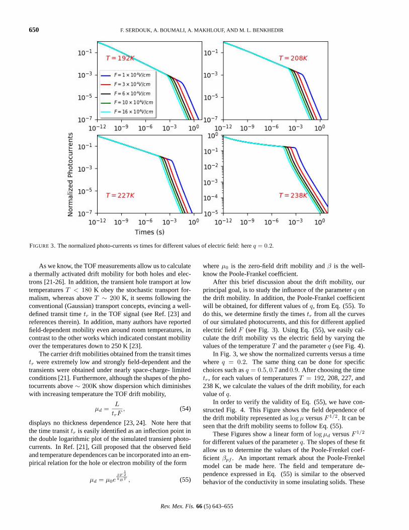
FIGURE 3. The normalized photo-currentsvstimes for different values of electric field: hereq = 0.2.

As we know, the TOF measurements allow us to calculatea thermally activated drift mobility for both holes and elec-trons [21-26]. In addition, the transient hole transport at lowtemperaturesT < 180 K obey the stochastic transport for-malism, whereas aboveT ∼ 200 K, it seems following theconventional (Gaussian) transport concepts, evincing a well-defined transit timetr in the TOF signal (see Ref. [23] andreferences therein). In addition, many authors have reportedfield-dependent mobility even around room temperatures, incontrast to the other works which indicated constant mobilityover the temperatures down to 250 K [23].

The carrier drift mobilities obtained from the transit timestr were extremely low and strongly field-dependent and thetransients were obtained under nearly space-charge- limitedconditions [21]. Furthermore, although the shapes of the pho-tocurrents above∼ 200K show dispersion which diminisheswith increasing temperature the TOF drift mobility,

µd =L

trF, (54)

displays no thickness dependence [23, 24]. Note here thatthe time transittr is easily identified as an inflection point inthe double logarithmic plot of the simulated transient photo-currents. In Ref. [21], Gill proposed that the observed fieldand temperature dependences can be incorporated into an em-pirical relation for the hole or electron mobility of the form

µd = µ0eβF

12

kBT , (55)

whereµ0 is the zero-field drift mobility andβ is the well-know the Poole-Frankel coefficient.

After this brief discussion about the drift mobility, ourprincipal goal, is to study the influence of the parameterq onthe drift mobility. In addition, the Poole-Frankel coefficientwill be obtained, for different values ofq, from Eq. (55). Todo this, we determine firstly the timestr from all the curvesof our simulated photocurrents, and this for different appliedelectric fieldF (see Fig. 3). Using Eq. (55), we easily cal-culate the drift mobility vs the electric field by varying thevalues of the temperatureT and the parameterq (see Fig. 4).

In Fig. 3, we show the normalized currents versus a timewhereq = 0.2. The same thing can be done for specificchoices such asq = 0.5, 0.7 and0.9. After choosing the timetr, for each values of temperaturesT = 192, 208, 227, and238 K, we calculate the values of the drift mobility, for eachvalue ofq.

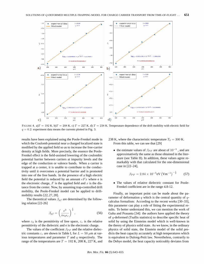
In order to verify the validity of Eq. (55), we have con-structed Fig. 4. This Figure shows the field dependence ofthe drift mobility represented aslog µ versusF 1/2. It can beseen that the drift mobility seems to follow Eq. (55).

These Figures show a linear form oflog µd versusF 1/2

for different values of the parameterq. The slopes of these fitallow us to determine the values of the Poole-Frenkel coef-ficient βpf . An important remark about the Poole-Frenkelmodel can be made here. The field and temperature de-pendence expressed in Eq. (55) is similar to the observedbehavior of the conductivity in some insulating solids. These

Rev. Mex. Fıs. 66 (5) 643–655

SOLUTIONS OFQ-DEFORMED MULTIPLE-TRAPPING MODEL FOR CHARGE CARRIER TRANSPORT FROM TIME-OF-FLIGHT . . . 651

FIGURE 4. a)T = 192 K. b)T = 208 K. c) T = 227 K. d) T = 238 K. Temperature dependence of the drift mobility with electric field forq = 0.2: experiment data means the currents plotted in Fig. 3.

results have been explained using the Poole-Frenkel mode inwhich the Coulomb potential near a charged localized state ismodified by the applied field so as to increase the free-carrierdensity at high fields. More precisely, the essence the Poole-Frenkel effect is the field-assisted lowering of the coulombicpotential barrier between carriers at impurity levels and theedge of the conduction or valence bands. When a carrier istrapped at a center, it is unable to contribute to the conduc-tivity until it overcomes a potential barrier and is promotedinto one of the free bands. In the presence of a high electricfield the potential is reduced by an amounteFx where e isthe electronic charge,F is the applied field andx is the dis-tance from the center. Now, by assuming trap-controlled driftmobility, the Poole-Frenkel model can be applied to drift-mobility results [22,27,28].

The theoretical valuesβpf are determined by the follow-ing relation [22-26]

βpf =(

e3

πε0εr

) 12

, (56)

whereε0 is the permittivity of free space,εr is the relativepermittivity of the dielectric and e is the electronic charge.

The values of the coefficientβPF and the relative dielec-tric constantsεr are shown in Table I, forL = 50 µm at var-ious temperatures and parameterT andq respectively. Therange of the temperatures areT = 192 K, 208 K, 227 K, and

238 K, where the characteristic temperatureT0 = 300 K.From this table, we can see that [29]

• the estimate values ofβPF are about of10−5 , and areapproximatively the same as those obtained in the liter-ature (see Table II). In addition, these values agree re-markably with that calculated for the one-dimensionalcase in [22–24],

βPF = 2.84× 10−5eV(Vm−1

)− 12 (57)

• The values of relative dielectric constant for Poole-Frenkel coefficient are in the range 4.8-12.

Finally, an important point can be made about the pa-rameter of deformationq which is the central quantity ofq-calculus formalism: According to the recent works [30–33],this parameter can play a role of fitting the experimental re-sults. To better understand this, we can mention the work ofGuha and Prasanta [34]: the authors have applied the theoryof q-deformed (Tsallis statistics) to describe specific heat ofsolid by using the Einsteins model which is well-known inthe theory of physics solid state. As we know, in the ordinaryphysics of solid state, the Einstein model of the solid pre-dicts the heat capacity accurately at high temperatures whichis equivalent to Dulong-Petit law. Nevertheless, contrarily tothe Debye model, the heat capacity noticeably deviates from

Rev. Mex. Fıs. 66 (5) 643–655

652 F. SERDOUK, A. BOUMALI, A. MAKHLOUF, AND M. L. BENKHEDIR

TABLE I. The estimate of the Poole-Frankel coefficientsβPF at some values of the temperatures and the parameterq

(a) q = 0.2 (b) q = 0.5

T (K) βpf

(10−5eV

(Vm−1

)− 12)

εr T (K) βpf

(10−5eV

(Vm−1

)− 12)

εr

192 2.55 9 192 2.55 8.63

208 2.4 10 208 2.40 10.81

227 2.3 11 227 2.30 10.64

238 2.35 10.5 238 2.35 11.17

(c) q = 0.7 (d) q = 0.9

192 2.53 9 192 2.57 8.81

208 2.43 9.86 208 2.35 10.55

227 2.15 12.53 227 2.14 12.70

238 2.21 11.87 238 2.12 13

TABLE II. Experimental values of some parameters.

References βPF

(10−5eV

(Vm−1

)− 12)

Relative permittivityεr estimated

Gill [22] 2.72 7.8

Marshallet al [23] 2.8 7.43

Kasapet al [24] 2.84 7.22

Benkhediret al [26] 2.6 8.61

experimental values at low temperatures. In this context, theauthors have been successful in solving this disagreementwhich appears at low temperature. They have studied thetemperature fluctuation effect via the fluctuation in the defor-mation parameterq. As a result, they found that, at low tem-perature, the Einstein curve of the specific heat in the Tsal-lis scenario exactly lies on the experimental data points andmatches with the Debye’s curve. In addition, they claim thata unique value of the Einstein temperatureθE , along with atemperature-dependent deformation parameterq (T ), can de-scribe the phenomenon of specific heat of solidi.e. the theoryis equivalent to Debye’s theory with a temperature-dependentθD.

In this direction, we can better understand the princi-pal aim of our contribution to this paper. Despite the non-existence of direct experimental verification of our model,we can claim that our approach,i.e., the introduction of theq-calculus formalism, can improve our understanding on thephysical behavior of charge carriers in amorphous semicon-ductors.

4. Conclusion

In this paper, we analyze multiple-trapping model (MTM) forcharge carrier transport from time-of-flight transient (TOF)photo-current in amorphous semiconductors in the general-ized non-extensive scenario (Tsallis statistics). This gener-alized statistical techniques (in Tsallis statisticsq being thedeformation parameter) have been applied to a wide rangeof complex systems. In our case, we have first discussed

the solutions of the (MTM) equations with the existence ofa linear form of an electrical field. The normalized cur-rents,I (s)/I (0), have been obtained by using a programthat we have developed in order to calculate the theoreticalcurrents. With this program, a good agreement between theexperimental and theoretical currents have been found (seeRef. [14]). Next, we considered the (MTM) equations in theframework of theq-calculus, the influence of the parameterqin the curves of the current have been well observed. Thesecurrents were obtained also by using the same program thathas used in the first case. Moreover, we studied the influenceof the parameterq of the q-calculus formalism on the driftmobility. It is shown that at low temperatures the drift mo-bility may be described by an empirical expression with thefollowing form µd = µ0e

β√

F/kbT . This form holds too inour case. Finally, the well-knownβpf , called Poole-Frankelcoefficient, are determined.

Appendix

A. q-calculus,q-product and q-sum

Here, we briefly describe some algebraic properties ofq-product andq-sum inq-calculus [19].

A.1 q-product

The definition of theq-product between two numbers is

x⊗q y =(x1−q + y1−q − 1

) 11−q

+, (x >, y > 0) (A.1)

Rev. Mex. Fıs. 66 (5) 643–655

SOLUTIONS OFQ-DEFORMED MULTIPLE-TRAPPING MODEL FOR CHARGE CARRIER TRANSPORT FROM TIME-OF-FLIGHT . . . 653

or, equivalently,

x⊗q y ≡ elnq x+lnq yq . (A.2)

Now, let us list some of its main properties:

• We recover the standard sum as a particular instance(q = 1), i.e.,

x⊗1 y = xy; (A.3)

• Commutative

x⊗q y = y ⊗q x (A.4)

• Additive underq-logarithm (hereafter referred to as ex-tensive),i.e.,

lnq (x⊗q y) = lnq x + lnq y; (A.5)

• Associative

x⊗q (y ⊗q z) = (x⊗q y)⊗q z = x⊗q y ⊗q z

=(x1−q + y1−q + z1−q − 2

) 11−q ; (A.6)

• The number one is the neutral element of theq-product

x⊗q 1 = x. (A.7)

• It has a (2 - q)-duality/inverse property,i.e.,

1(x⊗q y)

=(

1x

)⊗2−q

(1y

); (A.8)

• It admits zero under certain conditions, more precisely,

x⊗q 0 =

{0 if (q≥1 andx≥0) or if (q < 1 and0≤x≤1),(x1−q − 1

) 11−q if q < 1 andx > 1

(A.9)

• It satisfies

x⊗ 1q

y =(x

1q ⊗2−q y

1q

)q

(A.10)

• By q-multiplyingn equal factors, we can define thenthq-power as follows:

x⊗nq = x⊗q x⊗q . . .⊗q x

=[nx1−q − (1− q)

] 11−q . (A.11)

A.2 q-sum

Analogously to theq-product, we can define theq-sum as

x⊕q y = x + y + (1− q)xy (A.12)

This q-sum has the following main properties:

• We recover the standard sum as a particular instance(q = 1), i.e.,

x⊕1 y = x + y (A.13)

• It is multiplicative underq-exponential,i.e.,

ex⊕qy = exqey

q (A.14)

• Commutative

x⊕q y = y ⊕q x (A.15)

• Associative

x⊕q (y ⊕q z) = (x⊕q y)⊕q z = x⊕qy⊕qz

= x + y + z + (1− q) (xy + yz + xz)

+ (1− q)2 xyz; (A.16)

• It satisfies the following generalization of the distribu-tive property of standard sum and product,i.e., ofa(x + y) = ax + ay:

a(x⊕q y) = (ax)⊕ q+a−1a

(ay) . (A.17)

• The neutral element of theq-sum is zero,

x⊕q 0 = x. (A.18)

We can define the opposite (or inverse additive) ofx (callingit ªqx) as the element that, whenq-summed withx, yieldsthe neutral element:x⊕q (ªqx) = 0. So, we have

ªqx =−x

1 + (1− q)x, x 6= − 1

1− q. (A.19)

So, from the last relation we can obtain that

xªq y = x⊕q (ªqy)

=x− y

1 + (1− q) y, y 6= − 1

1− q. (A.20)

Theq-difference obeys:

Rev. Mex. Fıs. 66 (5) 643–655

654 F. SERDOUK, A. BOUMALI, A. MAKHLOUF, AND M. L. BENKHEDIR

• xªq y = ªqy⊕qx,

• xªq (y ªq z) = (xªq y)ªq z,

• buta (xªq y) 6= axªq ay.

Interesting cross properties emerge from theq-generalizations of the product and of the sum, for instance

lnq (xy) = lnq x⊕ lnq y, (A.21)

lnq (x⊗q y) = lnq x + lnq y, (A.22)

and, consistently,

ex+yq = ex

q ⊗ eyq , (A.23)

ex⊕qyq = ex

qeyq . (A.24)

While both theq-sum and theq-product are mathematicallyinteresting structures, they play a quite different role withinthe deep structure of the non-extensive theory. Theq-productreflects an essential property, namely, the extensivity of theentropy in the presence of special global correlations. Theq-sum instead only reflects how the entropies would composeif the subsystems were independent, even if we know that insuch a case we only actually needq = 1.

Acknowledgments

It is a great pleasure for the authors to thank the refereefor helpful comments. This work was fully supported bythe “Direction Generale de la Recherche Scientifique et duDeveloppement Technologique (DGRSDT)” of Algeria.

1. D. Bonatsos, L. Brito, D. Menezes, C. Providencia, and J. daProvidencia, Theq-deformed Moszkowski model: RPA modes,J. Phys. A26 (1993) 895,https://doi.org/10.1088/0305-4470/26/4/016 .

2. L. C. Biedenharn, The quantum groupSUq(2) and a q-analogue of the boson operators,J. Phys. A 22 (1989)L873, https://doi.org/10.1088/0305-4470/22/18/004 .

3. A. J. Macfarlane, Onq-analogues of the quantum harmonic os-cillator and the quantum groupSU(2)q, J. Phys. A22 (1989)4581, https://doi.org/10.1088/0305-4470/22/21/020 .

4. P. P. Kulish and E. V. Damaskinsky, On the q oscillatorand the quantum algebrasuq(1, 1), J. Phys. A23 (1990)L415, https://doi.org/10.1088/0305-4470/23/9/003 .

5. Y. J. Ng, Comment on the q-analogues of the harmonic oscil-lator, J. Phys. A23 (1990) 1023,https://doi.org/10.1088/0305-4470/23/6/022 .

6. H. Ui and N. Aizawa, q-Analogue of Boson Commuta-tor and the Quantum GroupsSUq(2) and SUq(1, 1), Mod.Phys. Lett. A5 (1990) 237,https://doi.org/10.1142/S0217732390000287 .

7. A. Boumali and H. Hassanabadi, The Statistical Propertiesof the q-Deformed Dirac Oscillator in One and Two Dimen-sions,Adv. High Energy Phys. 2017(2017) 9371391,https://doi.org/10.1155/2017/9371391 .

8. M. A. Kastner, Dielectric relaxation and delayed-collectionfield experiments in amorphous semiconductors,Solid StateCommun. 45 (1983) 191,https://doi.org/10.1016/0038-1098(83)90374-5 .

9. F. W. Schmidlin, Kinetic theory of hopping transport,Phi-los. Mag. B41(1980) 535,https://doi.org/10.1080/13642818008245405 .

10. F. W. Schmidlin, Theory of trap-controlled transient photocon-duction,Phys. Rev. B16 (1977) 2362,https://doi.org/10.1103/PhysRevB.16.2362 .

11. J. Noolandi, Multiple-trapping model of anomalous transit-time disperion ina-Se,Phys. Rev. B16 (1977) 4466,https://doi.org/10.1103/PhysRevB.16.4466 .

12. A. Ohno, J. Hanna, and D. H. Dunlap, Analysis of Trap Distri-bution Using Time-of- Flight Spectroscopy,Jpn. J. Appl. Phys.47 (2008) 1079, https://doi.org/10.1143/JJAP.47.1079 .

13. H. Naito, J. Ding, and M. Okuda, Determination of localizad-state distributions in amorphous semiconductors from transientphotoconductivity,Appl. Phys. Lett.64 (1994) 1830,https://doi.org/10.1063/1.111769 .

14. H. Naito et al., Density of states in amorphous semi-conductors determined from transient photoconductivity ex-periment: Computer simulation and experiment,J. Non-Cryst. Solids198-200(1996) 363,https://doi.org/10.1016/0022-3093(95)00725-3 .

15. T. Nagase and H. Naito, Determination of free carrier recom-bination lifetime in amorphous semiconductors: application tothe study of iodine doping effect in arsenic triselenide,J. Non-Cryst. Solids227-230(1998) 824,https://doi.org/10.1016/S0022-3093(98)00163-X .

16. N. Ogawa, T. Nagase, and H. Naito, Improvement of energyresolution of transient photoconductivity analysis for measur-ing localized-state distributions in amorphous semiconductors,J. Non-Cryst. Solids266-269 (2000) 367,https://doi.org/10.1016/S0022-3093(99)00732-2 .

17. A. Lavagno and G. Gervino, Quantum mechanics inq-deformed calculus,J. Phys. Conf. Ser.174 (2009) 012071,https://doi.org/10.1088/1742-6596/174/1/012071 .

18. F. Serdouk and M. L. Benkhedir, Density of states in pureand As doped amorphous selenium determined from transientphotoconductivity using Laplace-transform method,Phys-ica B 459 (2015) 122,https://doi.org/10.1016/j.physb.2014.12.002 .

Rev. Mex. Fıs. 66 (5) 643–655

SOLUTIONS OFQ-DEFORMED MULTIPLE-TRAPPING MODEL FOR CHARGE CARRIER TRANSPORT FROM TIME-OF-FLIGHT . . . 655

19. C. Tsallis,Introduction to Nonextensive Statistical Mechanics(Springer-Verlag, New York, 2009),https://doi.org/10.1007/978-0-387-85359-8 .

20. C. Tsallis and D. J. Bukman, Anomalous diffusion in the pres-ence of external forces: Exact time-dependent solutions andtheir thermostatical basis,Phys. Rev. E54 (1996) R2197(R),https://doi.org/10.1103/PhysRevE.54.R2197 .

21. W. E. Spear, The Hole Mobility in Selenium,Proc.Phys. Soc. 76 (1960) 826,https://doi.org/10.1088/0370-1328/76/6/302 .

22. W. D. Gill, Drift mobilities in amorphous charge-transfer com-plexes of trinitrofluorenone and poly-n-vinylcarbazole,J. Appl.Phys. 43 (1972) 5033,https://doi.org/10.1063/1.1661065 .

23. J. M. Marshall and A. E. Owen, The hole drift mobility of vit-reous selenium,Phys. Status Solidi A12 (1972) 181,https://doi.org/10.1002/pssa.2210120119 .

24. S. O. Kasap and C. Juhasz, Time-of-flight drift mobility mea-surements on chlorinedoped amorphous selenium films,J.Phys. D 18 (1985) 703,https://doi.org/10.1088/0022-3727/18/4/015 .

25. B. Fogal and S. Kasap, Temperature dependence of chargecarrier ranges in stabilized a-Se photoconductors,Can. J.Phys. 92 (2014) 634, https://doi.org/10.1139/cjp-2013-0524 .

26. M. L. Benkhedir, M. S. Aida, and G. J. Adriaenssens, Defectlevels in the band gap of amorphous selenium,J. Non-Cryst.Solids 344 (2004) 193, https://doi.org/10.1139/cjp-2013-0524 .

27. J. Frenkel, On Pre-Breakdown Phenomena in Insulators andElectronic Semi- Conductors,Phys. Rev.54 (1938) 647,https://doi.org/10.1103/PhysRev.54.647 .

28. R. M. Hill, Poole-Frenkel conduction in amorphous solids,Phi-los. Mag. 23 (1971) 59, https://doi.org/10.1080/14786437108216365 .

29. M. Anwar, I. M. Ghauri, and S. A. Siddiqi, The Electrical Prop-erties of Amorphous Thin Films of Al-In2O3-Al Structure De-posited by Thermal Evaporation,Rom J. Phys. 50 (2005) 763.

30. S. Kim, W. S. Chung, and H. Hassanabadi, q-deformed Gammafunction,q-deformed probability distributions andq-deformedstatistical physics based on Tsallis’sq-exponential function,Eur. Phys. J. Plus134(2019) 572,https://doi.org/10.1140/epjp/i2019-13082-4 .

31. W. S. Chung and H. Hassanabadi, Fermi energy inthe q-deformed quantum mechanics,Mod. Phys. Lett.A 35 (2020) 2050074,https://doi.org/10.1142/S0217732320500741 .

32. W. S. Chung and H. Hassanabadi, Blackbody radiation andDebye model based on qdeformed bosonic Newton oscilla-tor algebra,Mod. Phys. Lett. A35 (2020) 2050147,https://doi.org/10.1142/S0217732320501473 .

33. W. S. Chung and H. Hassanabadi, q-Deformed Quan-tum Mechanics Based on the q- Addition,Fortschr. Phys.67(2019) 1800111https://doi.org/10.1002/prop.201800111 .

34. A. Guha and P. K. Das, Constraints on light Dark Matterfermions from relic density consideration and Tsallis statistics,J. High Energy Phys.2018(2018) 139,https://doi.org/10.1007/JHEP06(2018)139 .

Rev. Mex. Fıs. 66 (5) 643–655