Solutions Classical Dynamics of Particles and Systems 5ed
496
CHAPTER 0 Contents Preface v Problems Solved in Student Solutions Manual vii 1 Matrices, Vectors, and Vector Calculus 1 2 Newtonian Mechanics—Single Particle 29 3 Oscillations 79 4 Nonlinear Oscillations and Chaos 127 5 Gravitation 149 6 Some Methods in The Calculus of Variations 165 7 Hamilton’s Principle—Lagrangian and Hamiltonian Dynamics 181 8 Central-Force Motion 233 9 Dynamics of a System of Particles 277 10 Motion in a Noninertial Reference Frame 333 11 Dynamics of Rigid Bodies 353 12 Coupled Oscillations 397 13 Continuous Systems; Waves 435 14 Special Theory of Relativity 461 iii
-
Upload
ricardo-vega -
Category
Documents
-
view
329 -
download
30
Transcript of Solutions Classical Dynamics of Particles and Systems 5ed
CHAPTER 0 Contents
Preface v
Problems Solved in Student Solutions Manual vii
1 Matrices, Vectors, and Vector Calculus 1
2 Newtonian Mechanics—Single Particle 29
3 Oscillations 79
4 Nonlinear Oscillations and Chaos 127
5 Gravitation 149
6 Some Methods in The Calculus of Variations 165
7 Hamilton’s Principle—Lagrangian and Hamiltonian Dynamics 181
8 Central-Force Motion 233
9 Dynamics of a System of Particles 277
10 Motion in a Noninertial Reference Frame 333
11 Dynamics of Rigid Bodies 353
12 Coupled Oscillations 397
13 Continuous Systems; Waves 435
14 Special Theory of Relativity 461
iii

iv CONTENTS
CHAPTER 0 Preface
This Instructor’s Manual contains the solutions to all the end-of-chapter problems (but not the appendices) from Classical Dynamics of Particles and Systems, Fifth Edition, by Stephen T. Thornton and Jerry B. Marion. It is intended for use only by instructors using Classical Dynamics as a textbook, and it is not available to students in any form. A Student Solutions Manual containing solutions to about 25% of the end-of-chapter problems is available for sale to students. The problem numbers of those solutions in the Student Solutions Manual are listed on the next page.
As a result of surveys received from users, I continue to add more worked out examples in the text and add additional problems. There are now 509 problems, a significant number over the 4th edition.
The instructor will find a large array of problems ranging in difficulty from the simple “plug and chug” to the type worthy of the Ph.D. qualifying examinations in classical mechanics. A few of the problems are quite challenging. Many of them require numerical methods. Having this solutions manual should provide a greater appreciation of what the authors intended to accomplish by the statement of the problem in those cases where the problem statement is not completely clear. Please inform me when either the problem statement or solutions can be improved. Specific help is encouraged. The instructor will also be able to pick and choose different levels of difficulty when assigning homework problems. And since students may occasionally need hints to work some problems, this manual will allow the instructor to take a quick peek to see how the students can be helped.
It is absolutely forbidden for the students to have access to this manual. Please do not give students solutions from this manual. Posting these solutions on the Internet will result in widespread distribution of the solutions and will ultimately result in the decrease of the usefulness of the text.
The author would like to acknowledge the assistance of Tran ngoc Khanh (5th edition), Warren Griffith (4th edition), and Brian Giambattista (3rd edition), who checked the solutions of previous versions, went over user comments, and worked out solutions for new problems. Without their help, this manual would not be possible. The author would appreciate receiving reports of suggested improvements and suspected errors. Comments can be sent by email to [email protected], the more detailed the better.
Stephen T. Thornton Charlottesville, Virginia
v
vi PREFACE
CHAPTER 1 Matrices, Vectors,
and Vector Calculus
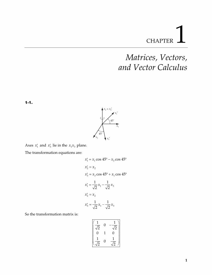
1-1.
x2 = x2!x1!
45˚
x1
x3!x3
45˚
Axes and lie in the plane. 1x 3x 1 3x x
The transformation equations are:
1 1 3cos 45 cos 45x x x
2 2x x
3 3 1cos 45 cos 45x x x
1 11 12 2
x x 3x
2 2x x
3 11 12 2
x x 3x
So the transformation matrix is:
1 10
2 20 1 01 1
02 2
1
2 CHAPTER 1
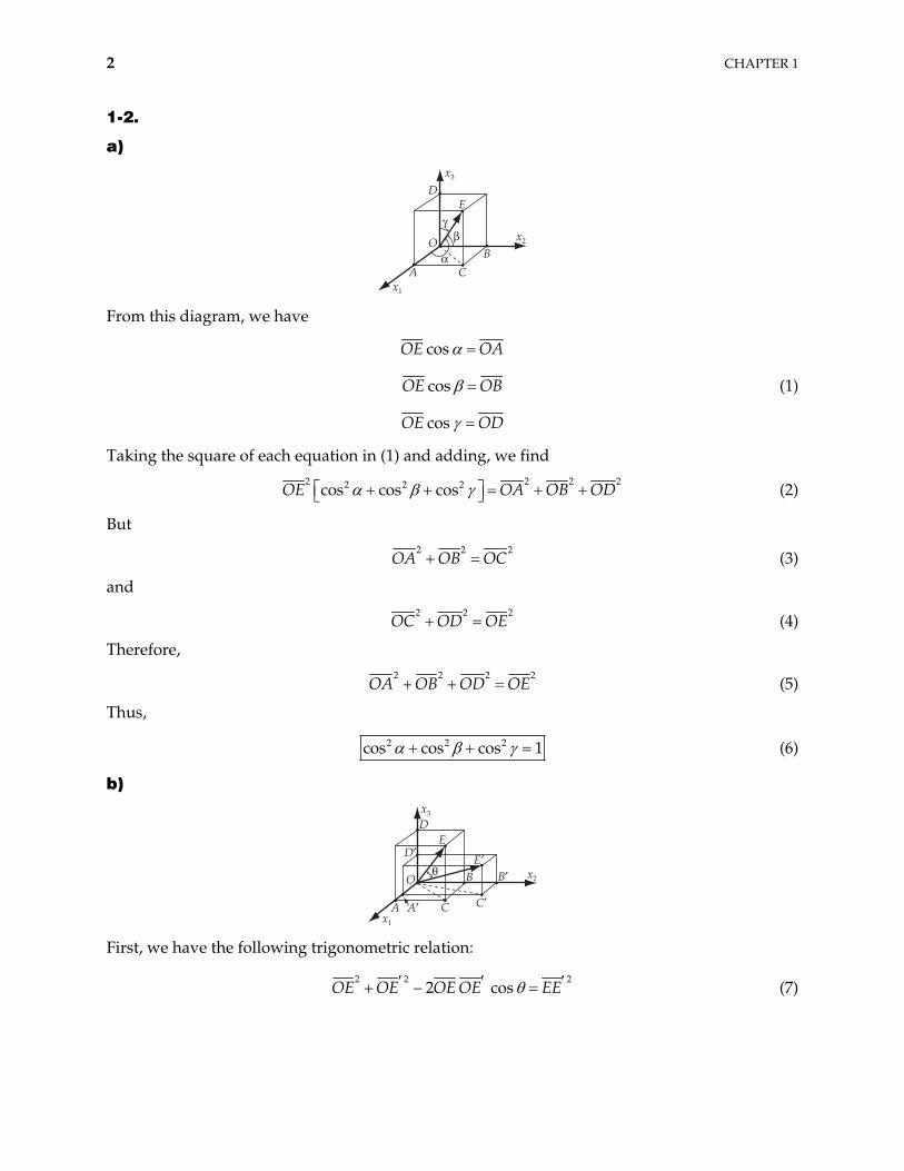
1-2.
a)
x1
A
B
C
D
"
#$
O
E
x2
x3
From this diagram, we have
cosOE OA
cosOE OB (1)
cosOE OD
Taking the square of each equation in (1) and adding, we find
2 2 2 2cos cos cos OA OB OD
2 2 2OE (2)
But
2 2
OA OB OC2 (3)
and
2 2
OC OD OE2
(4)
Therefore,
2 2 2
OA OB OD OE2 (5)
Thus,
2 2 2cos cos cos 1 (6)
b)
x3
A A!x1
x2O
ED
C
B%
C!
B!E!D!
First, we have the following trigonometric relation:
2 2
2 cosOE OE OE OE EE2
(7)

MATRICES, VECTORS, AND VECTOR CALCULUS 3
But,
2 2 22
2 2
2
cos cos cos cos
cos cos
EE OB OB OA OA OD OD
OE OE OE OE
OE OE (8)
or,
2 2 22 2 2 2 2 2
2 2
cos cos cos cos cos cos
2 cos cos cos cos cos cos
2 cos cos cos cos cos cos
EE OE OE
OE OE
OE OE OE OE (9)
Comparing (9) with (7), we find
cos cos cos cos cos cos cos (10)
1-3.
x1e3!
x2
x3
O
e1e2
e3
A e2!
e1!e2
e1
e3
Denote the original axes by , , , and the corresponding unit vectors by e , , . Denote the new axes by , , and the corresponding unit vectors by
1x 2x 3x 1 2e 3e
1x 2x 3x 1e , 2e , e . The effect of the rotation is e e , , e . Therefore, the transformation matrix is written as:
3
1 3 2 1e e 3 2e
1 1 1 2 1 3
2 1 2 2 2 3
3 1 3 2 3 3
cos , cos , cos , 0 1 0cos , cos , cos , 0 0 1
1 0 0cos , cos , cos ,
e e e e e e
e e e e e e
e e e e e e
1-4.
a) Let C = AB where A, B, and C are matrices. Then,
ij ik kjk
C A B (1)
tji jk ki ki jkij
k k
C C A B B A
4 CHAPTER 1
Identifying tki ik
BB and tjk kj
A A ,
t ti
tj ik kj
k
C B A (2)
or,
ttC AB B At t (3)
b) To show that 1 1 1AB B A ,
1 1 1 1AB B A I B A AB (4)
That is,
1 1 1 1AB B A AIA AA I (5)
1 1 1 1B A AB B IB B B I (6)
1-5. Take to be a two-dimensional matrix:
11 1211 22 12 21
21 22
(1)
Then,
2 2 2 2 2 2 2 2 2 2 2 2 211 22 11 22 12 21 12 21 11 21 12 22 11 21 12 22
2 2 2 2 2 2 2 2 2 222 11 12 21 11 12 11 21 11 22 12 21 12 22
22 2 2 211 12 22 21 11 21 12 22
2
2
(2)
But since is an orthogonal transformation matrix, ij kj ikj
.
Thus,
2 2 2 211 12 21 22
11 21 12 22
1
0 (3)
Therefore, (2) becomes
2 1 (4)
1-6. The lengths of line segments in the jx and jx systems are
2j
j
L x ; 2i
i
L x (1)
MATRICES, VECTORS, AND VECTOR CALCULUS 5
If , then L L
2 2j i
j i
x x (2)
The transformation is
i ij jj
x x (3)
Then,
(4)
2
,
j ik kj i k
k ik ik i
x x
x x
i x
But this can be true only if
ik i ki
(5)
which is the desired result.
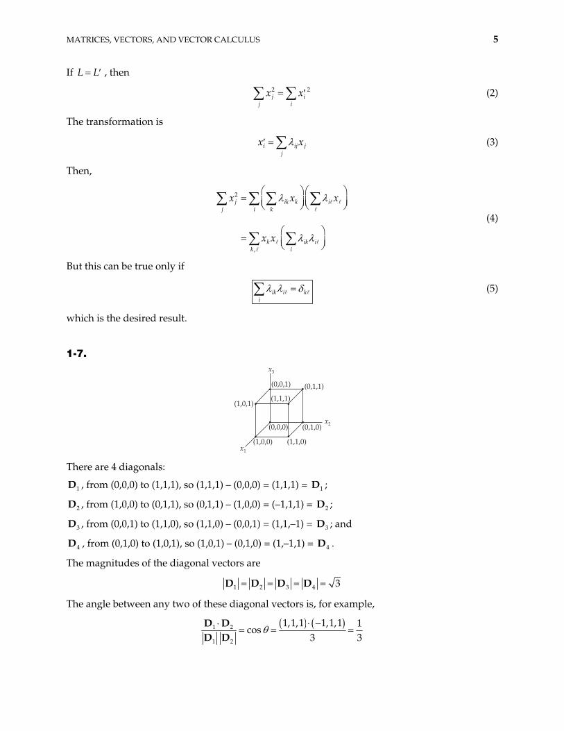
1-7.
x1
(1,0,1)
x3
x2
(1,0,0) (1,1,0)
(0,1,0)
(1,1,1)
(0,0,1) (0,1,1)
(0,0,0)
There are 4 diagonals:
1D , from (0,0,0) to (1,1,1), so (1,1,1) – (0,0,0) = (1,1,1) = D ; 1
2D , from (1,0,0) to (0,1,1), so (0,1,1) – (1,0,0) = (–1,1,1) = ; 2D
3D , from (0,0,1) to (1,1,0), so (1,1,0) – (0,0,1) = (1,1,–1) = ; and 3D
4D , from (0,1,0) to (1,0,1), so (1,0,1) – (0,1,0) = (1,–1,1) = D . 4
The magnitudes of the diagonal vectors are
1 2 3 4 3D D D D
The angle between any two of these diagonal vectors is, for example,
1 2
1 2
1,1,1 1,1,1 1cos
3 3D DD D
6 CHAPTER 1
so that
1 1cos 70.5
3
Similarly,
1 3 2 3 3 41 4 2 4
1 3 1 4 2 3 2 4 3 4
13
D D D D D DD D D DD D D D D D D D D D
1-8. Let be the angle between A and r. Then, 2AA r can be written as
2cosAr A
or,
cosr A (1)
This implies
2
QPO (2)
Therefore, the end point of r must be on a plane perpendicular to A and passing through P.
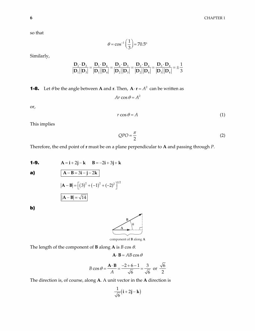
1-9. 2A i j k 2 3B i j k
a) 3 2A B i j k
1 22 2 23 1 ( 2)A B
14A B
b)
component of B along A
B
A%
The length of the component of B along A is B cos .
cosABA B
2 6 1 3 6
cos or26 6A
A BB
The direction is, of course, along A. A unit vector in the A direction is
1
26
i j k
MATRICES, VECTORS, AND VECTOR CALCULUS 7
So the component of B along A is
1
22
i j k
c) 3 3cos
6 14 2 7ABA B
; 1 3cos
2 7
71
d) 2 1 1 1 1 2
1 2 13 1 2 1 2 3
2 3 1
i j kA B i j k
5 7A B i j k
e) 3 2A B i j k 5A B i j
3 11 5 0
i j kA B A B 2
10 2 14A B A B i j k
1-10. 2 sin cosb t b tr i j
a) 2 2
2 cos sin
2 sin cos
b t b t
b t b t 2
v r i j
a v i j r
1 22 2 2 2 2 2
1 22 2
speed 4 cos sin
4 cos sin
b t b
b t t
tv
1 22speed 3 cos 1b t
b) At 2t , sin 1t , cos 0t
So, at this time, bv j , 22ba i
So, 90
8 CHAPTER 1
1-11.
a) Since ijk j kijk
A BA B , we have
,
1 2 3 3 2 2 1 3 3 1 3 1 2 2 1
1 2 3 1 2 3 1 2 3
1 2 3 1 2 3 1 2 3
1 2 3 1 2 3 1 2 3
( ) ijk j k ii j k
A B C
C A B A B C A B A B C A B A B
C C C A A A A A AA A A C C C B B BB B B B B B C C C
A B C
A B C
(1)
We can also write
1 2 3 1 2 3
1 2 3 1 2 3
1 2 3 1 2 3
( )C C C B B BB B B C C CA A A A A A
A B C B C A (2)
We notice from this result that an even number of permutations leaves the determinant unchanged.
b) Consider vectors A and B in the plane defined by e , . Since the figure defined by A, B, C is a parallelepiped, area of the base, but
1
3
2e
3A B e e C altitude of the parallelepiped. Then,
3 area of the base
= altitude area of the base
= volume of the parallelepiped
C A B C e
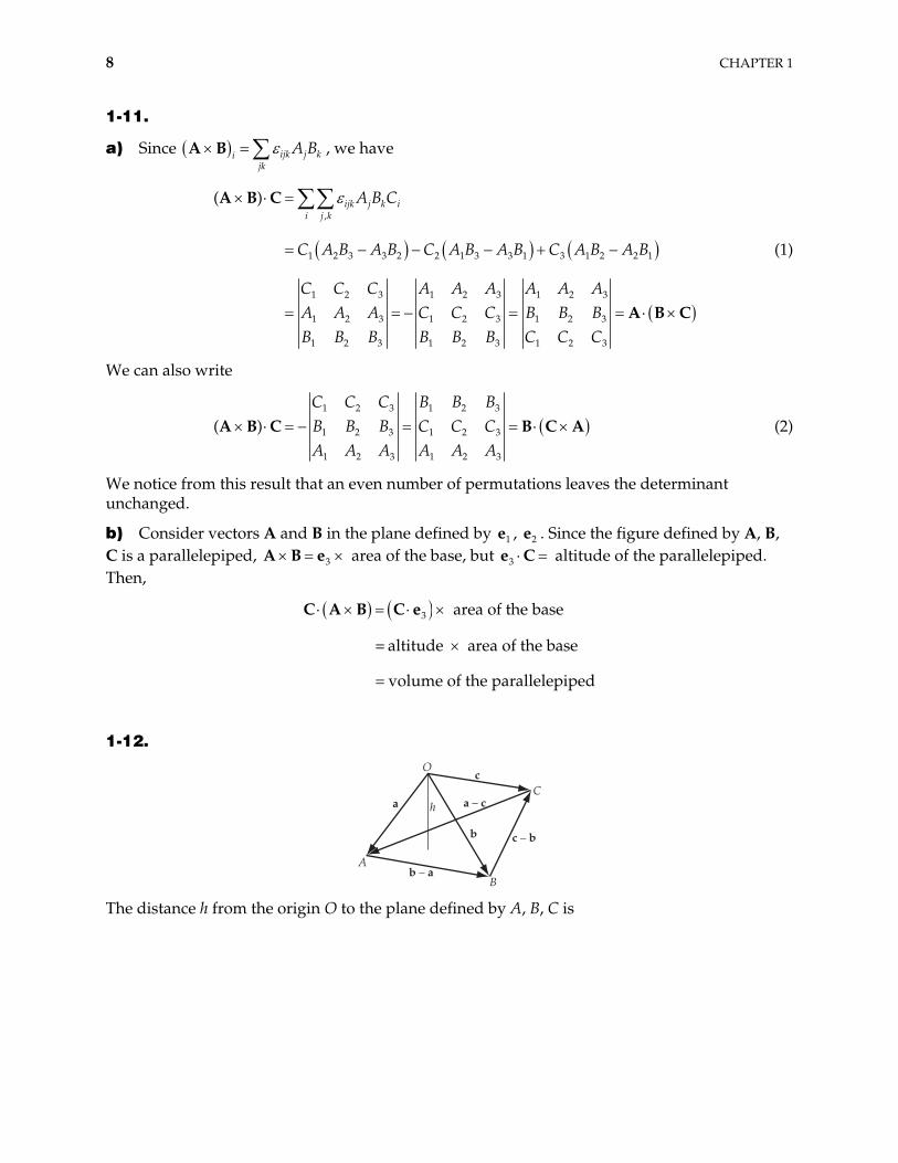
1-12.
O
A
B
Cha
b
c
a – c
c – b
b – a
The distance h from the origin O to the plane defined by A, B, C is
MATRICES, VECTORS, AND VECTOR CALCULUS 9
ha b a c b
b a c b
a b c a c a bb c a c a b
a b ca b b c c a
(1)
The area of the triangle ABC is:
1 1 12 2 2
b a c b a c b a c b a cA (2)
1-13. Using the Eq. (1.82) in the text, we have
2AA A X X A A A A X A XA B
from which
2AB A A
X
1-14.
a) 1 2 1 2 1 0 1 2 10 3 1 0 1 2 1 2 92 0 1 1 1 3 5 3 3
AB
Expand by the first row.
2 9 1 9 1 2
1 2 13 3 5 3 5 3
AB
104AB
b) 1 2 1 2 1 9 70 3 1 4 3 13 92 0 1 1 0 5 2
AC
9 7
13 95 2
AC
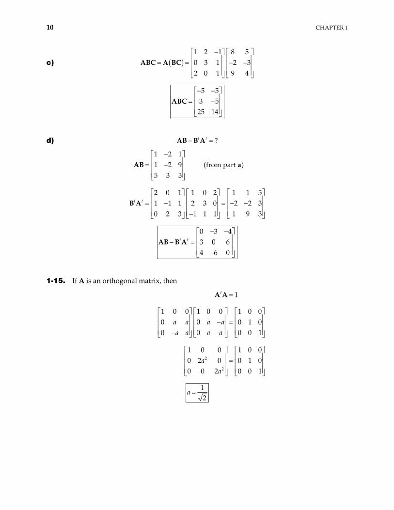
10 CHAPTER 1
c) 1 2 1 8 50 3 1 2 32 0 1 9 4
ABC A BC
5 5
3 525 14
ABC
d) ?t tAB B A
1 2 11 2 9 (from part )5 3 3
2 0 1 1 0 2 1 1 51 1 1 2 3 0 2 2 30 2 3 1 1 1 1 9 3
t t
AB a
B A
0 3 43 0 64 6 0
t tAB B A
1-15. If A is an orthogonal matrix, then
2
2
1
1 0 0 1 0 0 1 0 00 0 0 10 0 0 0
1 0 0 1 0 00 2 0 0 1 00 0 2 0 0 1
t
a a a aa a a a
aa
01
A A
12
a
MATRICES, VECTORS, AND VECTOR CALCULUS 11
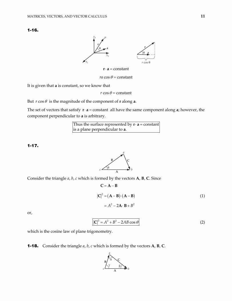
1-16.
x3 P
r%
x2
x1
a
r
% a
r cos % constantr a
cos constantra
It is given that a is constant, so we know that
cos constantr
But cosr is the magnitude of the component of r along a.
The set of vectors that satisfy all have the same component along a; however, the component perpendicular to a is arbitrary.
constantr a
This
us the surface represented by constant a plane perpendicular to .
r aa
1-17.
a
A%
b
B
c
C
Consider the triangle a, b, c which is formed by the vectors A, B, C. Since
2
2 22A B
C A B
C A B A B
A B
(1)
or,
2 2 2 2 cosA B ABC (2)
which is the cosine law of plane trigonometry.
1-18. Consider the triangle a, b, c which is formed by the vectors A, B, C.
A
" CB
$ #bc
a
12 CHAPTER 1
C A B (1)
so that
C B A B B (2)
but the left-hand side and the right-hand side of (2) are written as:
3sinBCC B e (3)
and
3sinABA B B A B B B A B e (4)
where e is the unit vector perpendicular to the triangle abc. Therefore, 3
sin sinBC AB (5)
or,
sin sin
C A
Similarly,
sin sin sin
C A B (6)
which is the sine law of plane trigonometry.
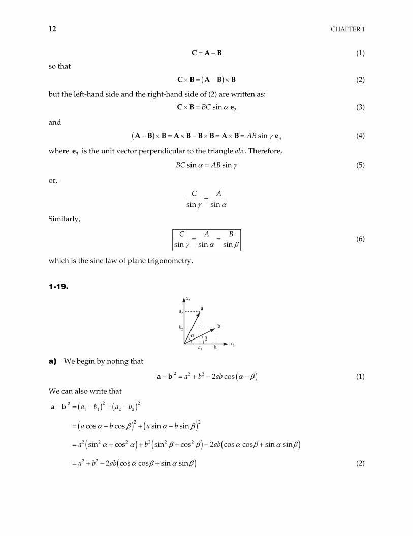
1-19.
x2
a
"x1
a2
b2
a1 b1
b
#
a) We begin by noting that
2 2 2 2 cosa b aba b (1)
We can also write that 2 22
1 1 2 2
2 2
2 2 2 2 2 2
2 2
cos cos sin sin
sin cos sin cos 2 cos cos sin sin
2 cos cos sin sin
a b a b
a b a b
a b ab
a b ab
a b
(2)
MATRICES, VECTORS, AND VECTOR CALCULUS 13
Thus, comparing (1) and (2), we conclude that
cos cos cos sin sin (3)
b) Using (3), we can find sin :
2
2 2 2 2
2 2 2 2
2 2 2 2
2
sin 1 cos
1 cos cos sin sin 2cos sin cos sin
1 cos 1 sin sin 1 cos 2cos sin cos sin
sin cos 2sin sin cos cos cos sin
sin cos cos sin (4)
so that
sin sin cos cos sin
j
(5)
1-20.
a) Consider the following two cases:
When i 0ij but 0ijk .
When i j 0ij but 0ijk .
Therefore,
0ijk ijij
(1)
b) We proceed in the following way:
When j = k, 0ijk ijj .
Terms such as 11 11 0j . Then,
12 12 13 13 21 21 31 31 32 32 23 23ijk jk i i i i i ijk
Now, suppose i , then, 1
123 123 132 132 1 1 2jk
14 CHAPTER 1
for , . For 2i 213 213 231 231 1 1 2jk
3i , 312 312 321 321 2jk
. But i = 1,
gives . Likewise for i = 2, 2 0jk
1 ; i = 1, 3 ; i = 3, 1 ; i = 2, ; i = 3, .
Therefore,
3 2
,
2ijk jk ij k
(2)
c) 123 123 312 312 321 321 132 132 213 213 231 231
1 1 1 1 1 1 1 1 1 1 1 1
ijk ijkijk
or,
6ijk ijkijk
(3)
1-21. ijk j kijk
A BA B (1)
ijk j k ii jk
A B CA B C (2)
By an even permutation, we find
ijk i j kijk
A B CABC (3)
1-22. To evaluate ijk mkk
we consider the following cases:
a) : 0 for all , ,ijk mk iik mkk k
i j i m
b) : 1 for
0 for
ijk mk ijk imkk k
i j
j m
and ,m k i j
i j
i
c) : 0 for
1 for and ,
ijk mk ijk ikk k
i m j
j k
d) : 0 for
1 for and ,
ijk mk ijk jmkk k
j m
m i k i j
MATRICES, VECTORS, AND VECTOR CALCULUS 15
e) : 0 for
1 for and ,
ijk mk ijk jkk k
j m i
i k i j
j k
m
f) : 0 for all , ,ijk mk ijk kk k
m i
g) : This implies that i = k or i = j or m = k. or i
Then, for all 0ijk mkk
, , ,i j m
h) for all or : 0ijk mkk
j m , , ,i j m
Now, consider i jm im j and examine it under the same conditions. If this quantity behaves in the same way as the sum above, we have verified the equation
ijk mk i jm im jk
a) : 0 for all , ,i im im ii j i m
b) : 1 if , ,
0 if
ii jm im jii j
j m
m i j m
c) : 1 if , ,
0 if
i ji ii ji m j i j
j
m i
d) : 1 if ,
0 if
i m imj i
i m
e) : 1 if ,
0 if
i mm im mj m i m
i
all , ,j
f) : 0 for i j il jm i
g) , : 0 for all , , ,i jm im ji m i j m
h) , : 0 for all , , ,i jm im ij m i j m
Therefore,
ijk mk i jm im jk
(1)
Using this result we can prove that
A B C A C B A B C
16 CHAPTER 1
First ijk j kijk
B CB C . Then,
mn m mn m njk j knmn mn jk
mn njk m j k mn jkn m j kjkmn jkmn
lmn jkn m j kjkm n
jl km k jm m j kjkm
m m m m m m m mm m m m
A B C A B C
A B C A B C
A B C
A B C
A B C A B C B A C C A B
B C
A B C
A C A B
Therefore,
A B C A C B A B C (2)
1-23. Write
j m mjm
A BA B
krs r skrs
C DC D
Then,
MATRICES, VECTORS, AND VECTOR CALCULUS 17
ijk j m m krs r sijk m rs
ijk j m krs m r sjk mrs
j m ijk rsk m r sj mrs k
j m ir js is jr m r sj mrs
j m m i j m i jj m
j m j m i j mj m j
A B C D
A B C D
A B C D
A B C D
A B C D A B D C
D A B C
A B C D
( ) ( )
j m im
i i
C A B D
C DABD ABC
Therefore,
( ) ( )A B C D ABD C ABC D
1-24. Expanding the triple vector product, we have
e A e A e e e A e (1)
But,
A e e A (2)
Thus,
A e A e e A e (3)
e(A · e) is the component of A in the e direction, while e (A e) is the component of A perpendicular to e.
18 CHAPTER 1
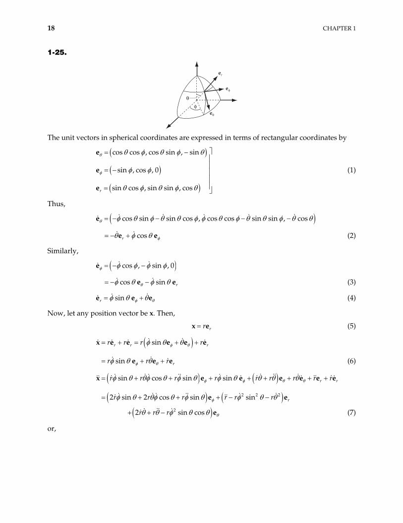
1-25.
er
e&
e%
%&
The unit vectors in spherical coordinates are expressed in terms of rectangular coordinates by
cos cos , cos sin , sin
sin , cos , 0
sin cos , sin sin , cosr
e
e
e
(1)
Thus,
cos sin sin cos , cos cos sin sin , cose
cosre (2) e
Similarly,
cos , sin , 0e
cos sin re (3) e
sinre e e (4)
Now, let any position vector be x. Then,
rrx e (5)
sin
sin
r r
r
r r r r
r r r
x e e e e e
e e e
r
(6)
2 2 2
2
sin cos sin sin
2 sin 2 cos sin sin
2 sin cos
r r
r
r r r r r r r r
r r r r r r
r r r
x e e e
e e
e
re e e
(7)
or,
MATRICES, VECTORS, AND VECTOR CALCULUS 19
2 2 2 2 2
2 2
1sin sin cos
1sin
sin
rd
r r r r rr dt
dr
r dt
x a e e
e (8)
1-26. When a particle moves along the curve
1 cosr k (1)
we have
2
sin
cos sin
r k
r k (2)
Now, the velocity vector in polar coordinates is [see Eq. (1.97)]
rr rv e e (3)
so that
22 2 2 2
2 2 2 2 2 2
2 2
sin 1 2 cos cos
2 2 cos
v r r
k k
k
v
(4)
and is, by hypothesis, constant. Therefore, 2v
2
22 1 cosv
k (5)
Using (1), we find
2vkr
(6)
Differentiating (5) and using the expression for r , we obtain
2 2
22 2
sin sin4 4 1 cos
v vr k
(7)
The acceleration vector is [see Eq. (1.98)]
2 2rr r r ra e e (8)
so that
20 CHAPTER 1
2
2 2
2 22 2
22
2
cos sin 1 cos
sincos 1 cos
2 1 cos
1 cos2 cos 1
2 1 cos
31 cos
2
r r r
k k
k
k
k
a e
(9)
or,
23
4rvk
a e (10)
In a similar way, we find
2 sin3
4 1 cosvk
a e (11)
From (10) and (11), we have
22ra a e a e (12)
or,
23 2
4 1 cosvk
a (13)
1-27. Since
r v r r r v r v r
we have
2 2
2
d ddt dt
r v
r v r r r v r v r
r r a r v v r v v v v r r a r
a r v v r r a (1)
Thus,
2rdt
r v r a r v v r r a v2d (2)
MATRICES, VECTORS, AND VECTOR CALCULUS 21
1-28. ln ln ii ix
grad r r e (1)
where
2i
i
xr (2)
Therefore,
2
2
1ln i
i ii
i
xx x
x
rr
r (3)
so that
21
ln i ii
xgrad r er
(4)
or,
2lnrr
grad r (5)
1-29. Let describe the surface S and 2 9r 12 1x y z describe the surface S . The angle
between and at the point (2,–2,1) is the angle between the normals to these surfaces at the point. The normal to is
2
1S 2S
1S
2 2 21
1 2 3 2, 2, 1
1 2 3
9 9
2 2 2
4 4 2
x y z
S r x y z
x y z
grad grad grad
e e e
e e e
2
(1)
In , the normal is: 2S
22
1 2 3 2, 2,
1 2 3
1
2
2
x 1y z
S x y z
z
grad grad
e e e
e e e
(2)
Therefore,
22 CHAPTER 1
1 2
1 2
1 2 3 1 2 3
cos
4 4 2 26 6
S SS S
grad gradgrad grad
e e e e e e (3)
or,
4
cos6 6
(4)
from which
1 6cos 74.2
9 (5)
1-30. 3
1i i
i ii i
i ii ii i
x x
x x
ixgrad e e
e e
Thus,
grad grad grad
1-31.
a)
1 23
2
1
12
2
12
2
2
22
n
n ni i j
i ji i
n
i i ji j
n
i i ji j
ni i
i
rr x
x x
nx x
x n x
x n r
grad e e
e
e
e (1)
Therefore,
2 nnr nrgrad r (2)
MATRICES, VECTORS, AND VECTOR CALCULUS 23
b)
3 3
1 1
1 2
2
1 2
2
i ii ii i
i ji ji
i i ji j
ii
i
f r f r rf r
x r
f rx
x r
f rx x
r
fxr dr
xgrad e e
e
e
e (3)
Therefore,
( )
f r
f rr rr
grad (4)
c)
1 22 22 2
2 2
1 2
2
1 2
2
1
2
2 1
2 2
22 22
ln ln ln
1 22
2
12 3
ji ji i
i jj
i i
jj
i ji ji
ii i j j
i j i ji
ji
rr x
x x
x x
xx
x xx
xx x x x
x
x rr
2
4 2 2
2 3 1rr r r
(5)
or,
22
1ln r
r (6)
24 CHAPTER 1
1-32. Note that the integrand is a perfect differential:
2 2d d
a b a bdt dt
r r r r r r r r (1)
Clearly,
2 22 2 cona b dt ar brr r r r st. (2)
1-33. Since
2
d r rdt r r r 2
rr
r r r r r (1)
we have
2
r ddt dt
r r dt rr r r
(2)
from which
2
rdt
r r rr r r
C (3)
where C is the integration constant (a vector).
1-34. First, we note that
ddt
A A A A A A (1)
But the first term on the right-hand side vanishes. Thus,
d
dt dtdt
A A A A (2)
so that
dtA A A A C (3)
where C is a constant vector.
MATRICES, VECTORS, AND VECTOR CALCULUS 25
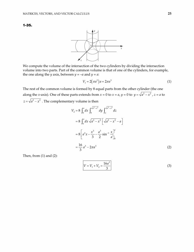
1-35.
x
z
y
We compute the volume of the intersection of the two cylinders by dividing the intersection volume into two parts. Part of the common volume is that of one of the cylinders, for example, the one along the y axis, between y = –a and y = a:
21 2 2V a a 3a (1)
The rest of the common volume is formed by 8 equal parts from the other cylinder (the one
along the x-axis). One of these parts extends from x = 0 to x = a, y = 0 to 2y a x2 , z = a to 2 2z a x . The complementary volume is then
2 2 2 2
2 0 0
2 2 2 2
0
3 32 1
0
3 3
8
8
8 sin3 2
162
3
a a x a x
a
a
a
V dx dy dz
dx a x a x a
x a xa x
a
a a (2)
Then, from (1) and (2):
3
1 216
3a
V V V (3)
26 CHAPTER 1
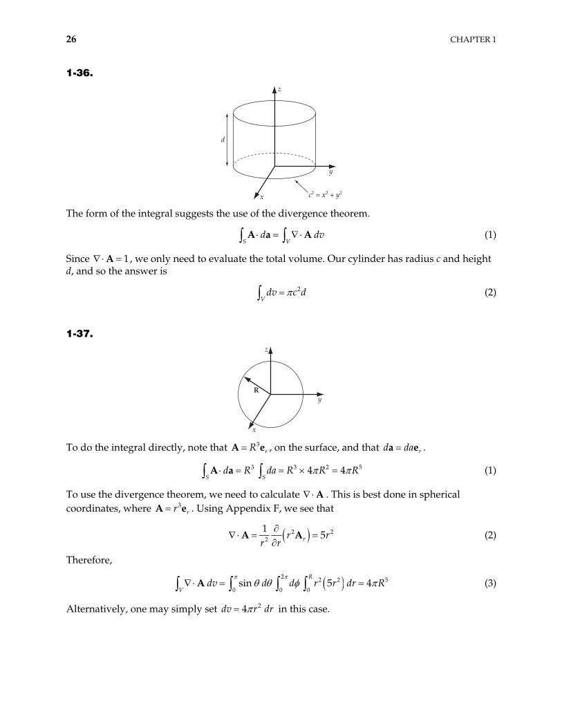
1-36.
d
z
x
y
c2 = x2 + y2
The form of the integral suggests the use of the divergence theorem.
(1) S V
dA a A dv
Since , we only need to evaluate the total volume. Our cylinder has radius c and height d, and so the answer is
1A
(2) 2
Vdv c d
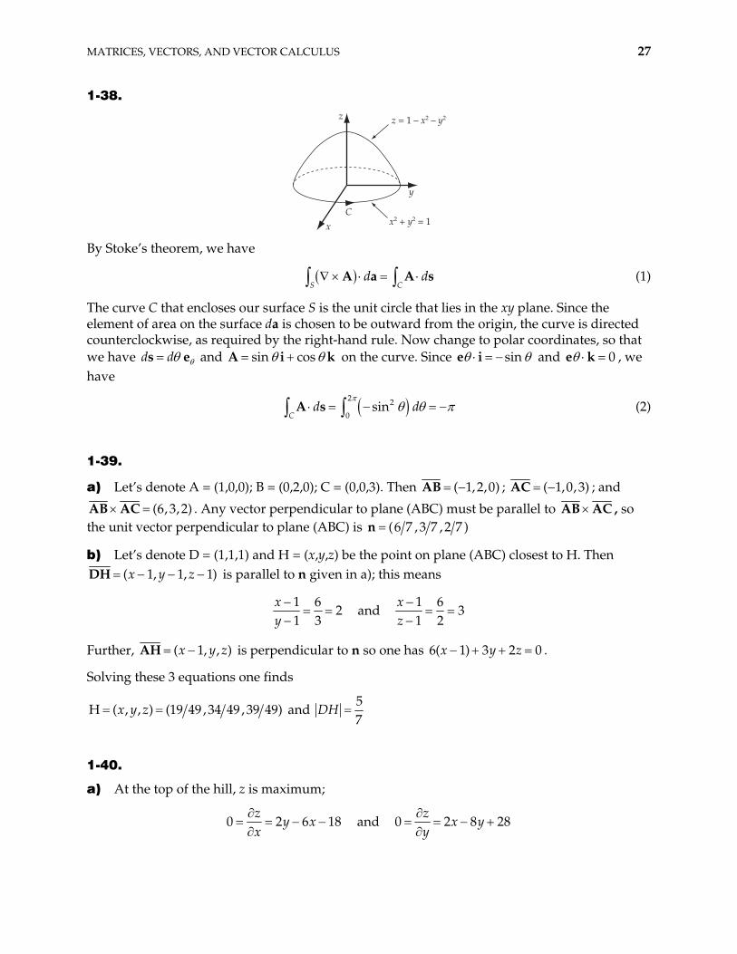
1-37.
z
y
x
R
To do the integral directly, note that A , on the surface, and that . 3rR e
5
rd daa e
3 3 24 4S S
d R da R R RA a (1)
To use the divergence theorem, we need to calculate A . This is best done in spherical coordinates, where A . Using Appendix F, we see that 3
rr e
22
15rr
r r2rA A (2)
Therefore,
2 2 2
0 0 0sin 5 4
R
Vdv d d r r dr R5A (3)
Alternatively, one may simply set dv in this case. 24 r dr
MATRICES, VECTORS, AND VECTOR CALCULUS 27
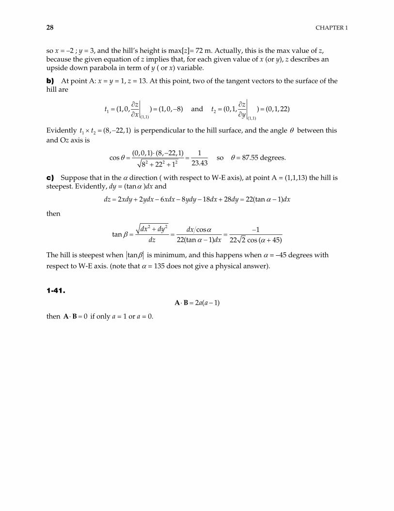
1-38.
x
z
y
Cx2 + y2 = 1
z = 1 – x2 – y2
By Stoke’s theorem, we have
S
dC
dA a A s (1)
The curve C that encloses our surface S is the unit circle that lies in the xy plane. Since the element of area on the surface da is chosen to be outward from the origin, the curve is directed counterclockwise, as required by the right-hand rule. Now change to polar coordinates, so that we have d ds e and sin cosA i k on the curve. Since sine i and 0e k , we have
2 2
0sin
Cd dA s (2)
1-39.
a) Let’s denote A = (1,0,0); B = (0,2,0); C = (0,0,3). Then ( 1, 2,0)AB ; ( 1,0, 3)AC ; and
(6, 3,2)AB AC . Any vector perpendicular to plane (ABC) must be parallel to AB AC , so the unit vector perpendicular to plane (ABC) is (6 7 ,3 7 , 2 7 )n
b) Let’s denote D = (1,1,1) and H = (x,y,z) be the point on plane (ABC) closest to H. Then ( 1, 1, 1x y zDH ) is parallel to n given in a); this means
1 6
21 3
xy
and 1 6
31 2
xz
Further, ( 1, ,x y )zAH is perpendicular to n so one has 6( 1) 3 2 0x y z .
Solving these 3 equations one finds
H ( , , ) (19 49,34 49, 39 49)x y z and 57
DH
1-40.
a) At the top of the hill, z is maximum;
0 2 and 6z
y xx
18 0 2 8z
x yy
28
28 CHAPTER 1
so x = –2 ; y = 3, and the hill’s height is max[z]= 72 m. Actually, this is the max value of z, because the given equation of z implies that, for each given value of x (or y), z describes an upside down parabola in term of y ( or x) variable.
b) At point A: x = y = 1, z = 13. At this point, two of the tangent vectors to the surface of the hill are
1(1,1)
(1,0, ) (1,0, 8)zx
t and 2(1,1)
(0,1, ) (0,1, 22)zy
t
Evidently t t is perpendicular to the hill surface, and the angle 1 2 (8, 22,1) between this and Oz axis is
2 2 2
(0,0,1) (8, 22,1) 1s
23.438 22 1co so = 87.55 degrees.
c) Suppose that in the direction ( with respect to W-E axis), at point A = (1,1,13) the hill is steepest. Evidently, dy = (tan )dx and
d 2 2 6 8 18 28 22(tan 1)z xdy ydx xdx ydy dx dy dx
then
2 2 cos 1
22(tan 1) 22 2 cos ( 45)dx dy dx
dz dxtan
The hill is steepest when tan is minimum, and this happens when = –45 degrees with respect to W-E axis. (note that = 135 does not give a physical answer).
1-41.
2 ( 1)a aA B
then if only a = 1 or a = 0. 0A B
CHAPTER 2 Newtonian Mechanics—
Single Particle
2-1. The basic equation is
i iF m x (1)
a) ,i iF x t f x g t m xi i : Not integrable (2)
b) ,i iF x t f x g t m xi i
ii idx
m f x gdt
t
i
i i
g tdxdt
f x m: Integrable (3)
c) ,i i i i iF x x f x g x m xi : Not integrable (4)
2-2. Using spherical coordinates, we can write the force applied to the particle as
r rF F FF e e e (1)
But since the particle is constrained to move on the surface of a sphere, there must exist a reaction force that acts on the particle. Therefore, the total force acting on the particle is r rF e
total F F mF e e r (2)
The position vector of the particle is
rRr e (3)
where R is the radius of the sphere and is constant. The acceleration of the particle is
rRa r e (4)
29
30 CHAPTER 2
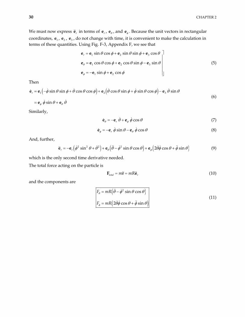
We must now express in terms of , re re e , and e . Because the unit vectors in rectangular coordinates, e , , e , do not change with time, it is convenient to make the calculation in terms of these quantities. Using Fig. F-3, Appendix F, we see that
1 2e 3
1 2 3
1 2 3
1 2
sin cos sin sin cos
cos cos cos sin sin
sin cos
re e e e
e e
e e e
e e (5)
Then
1 2sin sin cos cos cos sin sin cos sin
sin
r 3e e e e
e e (6)
Similarly,
cosre e e (7)
sin cosre e e (8)
And, further,
2 2 2 2sin sin cos 2 cos sinr re e e e (9)
which is the only second time derivative needed.
The total force acting on the particle is
total rm mRF r e (10)
and the components are
2 sin cos
2 cos sin
F mR
F mR (11)
NEWTONIAN MECHANICS—SINGLE PARTICLE 31
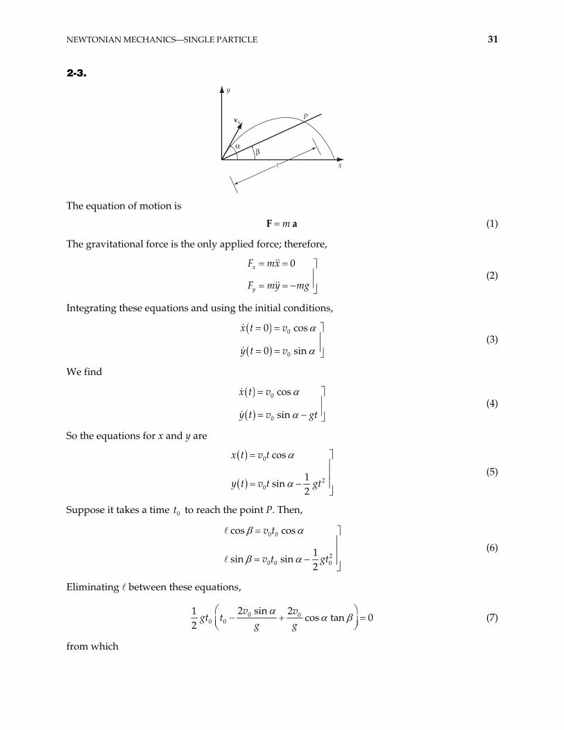
2-3.
y
x
v0P
!"
!
The equation of motion is
mF a (1)
The gravitational force is the only applied force; therefore,
0x
y
F mx
F my mg (2)
Integrating these equations and using the initial conditions,
0
0
0 cos
0 sin
x t v
y t v (3)
We find
0
0
cos
sin
x t v
y t v gt (4)
So the equations for x and y are
0
20
cos
1sin
2
x t v t
y t v t gt (5)
Suppose it takes a time t to reach the point P. Then, 0
0 0
20 0 0
cos cos
1sin sin
2
v t
v t gt (6)
Eliminating between these equations,
0 00 0
2 sin 21cos tan 0
2v v
tg g
gt (7)
from which
32 CHAPTER 2
00
2sin cos tan
vt
g (8)
2-4. One of the balls’ height can be described by 20 0 2y y v t gt . The amount of time it
takes to rise and fall to its initial height is therefore given by 02v g . If the time it takes to cycle the ball through the juggler’s hands is 0.9 s , then there must be 3 balls in the air during that time . A single ball must stay in the air for at least 3 , so the condition is 02 3v g , or
. 10 13.2 m sv
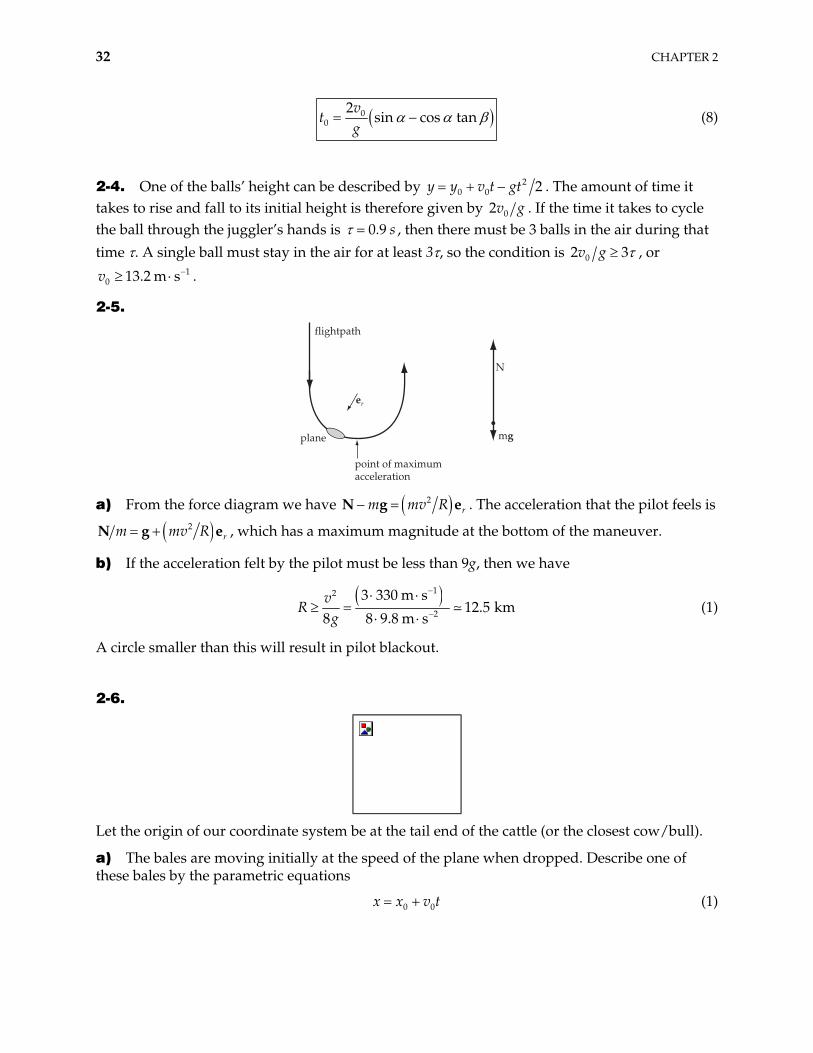
2-5.
mg
N
point of maximumacceleration
flightpath
plane
er
a) From the force diagram we have 2rm mv RN g e . The acceleration that the pilot feels is
2rm mv RN g e , which has a maximum magnitude at the bottom of the maneuver.
b) If the acceleration felt by the pilot must be less than 9g, then we have
12
2
3 330 m s12.5 km
8 8 9.8 m sv
Rg
(1)
A circle smaller than this will result in pilot blackout.
2-6.
Let the origin of our coordinate system be at the tail end of the cattle (or the closest cow/bull).
a) The bales are moving initially at the speed of the plane when dropped. Describe one of these bales by the parametric equations
0 0x x v t (1)
NEWTONIAN MECHANICS—SINGLE PARTICLE 33
20
12
y y gt (2)
where , and we need to solve for . From (2), the time the bale hits the ground is 0 80 my 0x
02y g . If we want the bale to land at 30 mx , then 0x x v0 . Substituting
and the other values, this gives -1s0 44.4 mv 0 210x m . The rancher should drop the bales 210 m behind the cattle.
b) She could drop the bale earlier by any amount of time and not hit the cattle. If she were late by the amount of time it takes the bale (or the plane) to travel by 30 m in the x-direction, then she will strike cattle. This time is given by 030 m 0.68 sv .
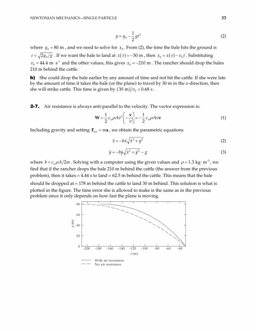
2-7. Air resistance is always anti-parallel to the velocity. The vector expression is:
21 12 2wc Av c Av
vv
W w v
a
(1)
Including gravity and setting , we obtain the parametric equations net mF
2x bx x y2 (2)
2 2y by x y g (3)
where 2w A mb c . Solving with a computer using the given values and , we find that if the rancher drops the bale 210 m behind the cattle (the answer from the previous problem), then it takes 4.44 s to land 62.5 m behind the cattle. This means that the bale
should be dropped at 178 m behind the cattle to land 30 m behind. This solution is what is plotted in the figure. The time error she is allowed to make is the same as in the previous problem since it only depends on how fast the plane is moving.
-31.3 kg m
–200 –180 –160 –140 –120 –100 –80 –60 –400
20
40
60
80
With air resistanceNo air resistance
x (m)
y (m
)
34 CHAPTER 2
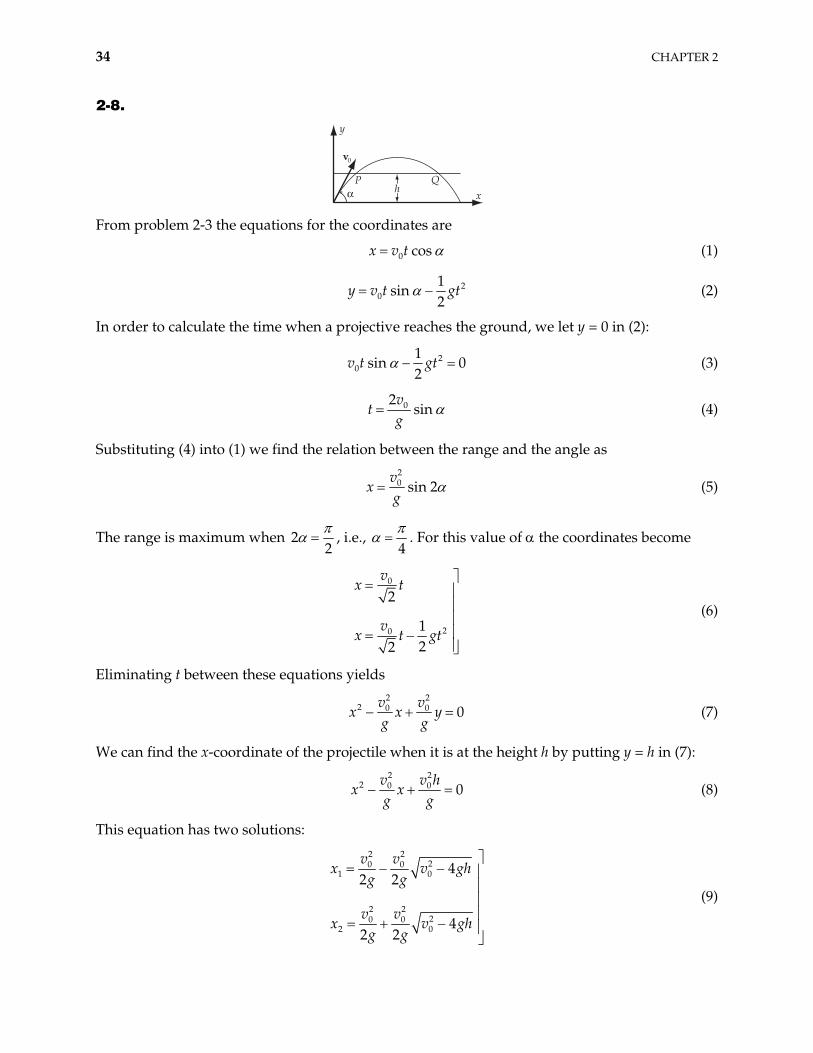
2-8.
P Qx
y
v0
! h
From problem 2-3 the equations for the coordinates are
0 cosx v t (1)
20
1sin
2y v t gt (2)
In order to calculate the time when a projective reaches the ground, we let y = 0 in (2):
20
1sin 0
2v t gt (3)
02sin
vt
g (4)
Substituting (4) into (1) we find the relation between the range and the angle as
20 sin 2
vx
g (5)
The range is maximum when 22
, i.e., 4
. For this value of the coordinates become
0
20
2
122
vx t
vx t gt
(6)
Eliminating t between these equations yields
2 2
2 0 0 0v v
x x yg g
(7)
We can find the x-coordinate of the projectile when it is at the height h by putting y = h in (7):
2 2
2 0 0 0v v h
x xg g
(8)
This equation has two solutions:
2 220 0
1 0
2 220 0
2 0
42 2
42 2
v vx v
g g
v vx v
g g
gh
gh
(9)
NEWTONIAN MECHANICS—SINGLE PARTICLE 35
where corresponds to the point P and to Q in the diagram. Therefore, 1x 2x
202 1 0 4
vd x x v gh
g (10)
2-9.
a) Zero resisting force ( ): 0rF
The equation of motion for the vertical motion is:
dv
F ma m mgdt
(1)
Integration of (1) yields
0v gt v (2)
where v is the initial velocity of the projectile and t = 0 is the initial time. 0
The time required for the projectile to reach its maximum height is obtained from (2). Since corresponds to the point of zero velocity,
mt
mt
00mv t v gtm , (3)
we obtain
0m
vt
g (4)
b) Resisting force proportional to the velocity rF kmv :
The equation of motion for this case is:
dv
F m mg kdt
mv (5)
where –kmv is a downward force for mt t and is an upward force for mt t . Integrating, we obtain
0 ktg kv gv t e
k k (6)
For t , v(t) = 0, then from (6), mt
0 1mktgv e
k (7)
which can be rewritten as
0ln 1mkv
ktg
(8)
Since, for small z (z 1) the expansion
36 CHAPTER 2
21 1ln 1
2 33z z z z (9)
is valid, (8) can be expressed approximately as
2
0 0 011
2 3 2mv kv kv
tg g g
(10)
which gives the correct result, as in (4) for the limit k 0.
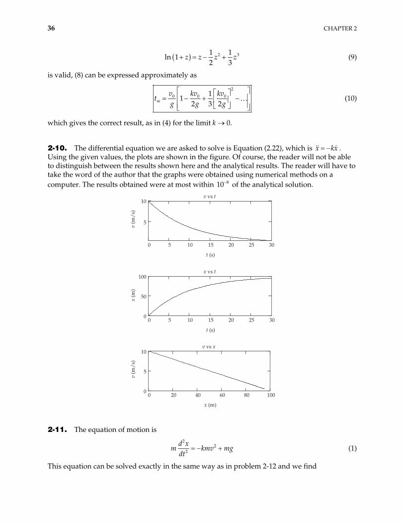
2-10. The differential equation we are asked to solve is Equation (2.22), which is . Using the given values, the plots are shown in the figure. Of course, the reader will not be able to distinguish between the results shown here and the analytical results. The reader will have to take the word of the author that the graphs were obtained using numerical methods on a computer. The results obtained were at most within 10
x kx
8 of the analytical solution.
0 5 10 15 20 25 30
5
10v vs t
t (s)
v (m
/s)
0 20 40 60 800
5
10
100
v vs x
x (m)
v (m
/s)
0 5 10 15 20 25 300
50
100x vs t
t (s)
x (m
)
2-11. The equation of motion is
2
22
d xm kmv mg
dt (1)
This equation can be solved exactly in the same way as in problem 2-12 and we find
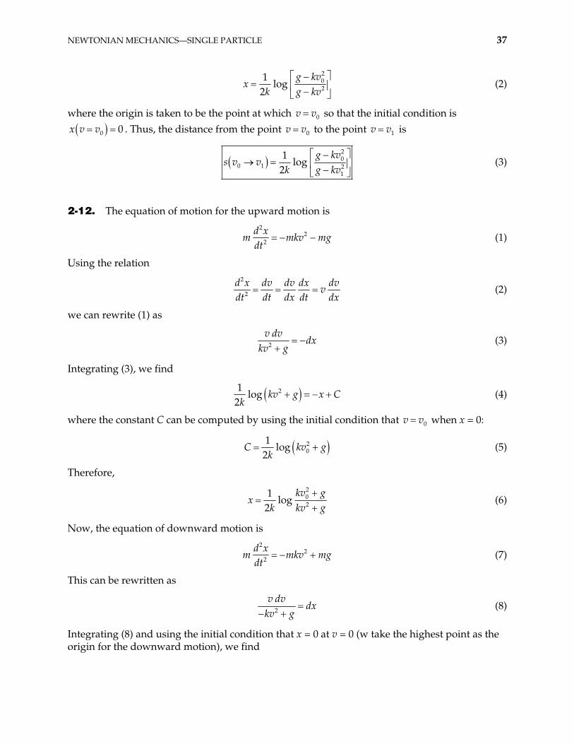
NEWTONIAN MECHANICS—SINGLE PARTICLE 37
202
1log
2g kv
xk g kv
(2)
where the origin is taken to be the point at which v 0v so that the initial condition is
0 0x v v . Thus, the distance from the point 0v v to the point v 1v is
20
0 1 21
1log
2g kv
s v vk g kv
(3)
2-12. The equation of motion for the upward motion is
2
22
d xm mkv
dtmg (1)
Using the relation
2
2
d x dv dv dx dvv
dt dt dx dt dx (2)
we can rewrite (1) as
2
v dvdx
kv g (3)
Integrating (3), we find
21log
2kv g x C
k (4)
where the constant C can be computed by using the initial condition that when x = 0: 0v v
20
1log
2C kv
kg (5)
Therefore,
202
1log
2kv g
xk kv g
(6)
Now, the equation of downward motion is
2
22
d xm mkv
dtmg (7)
This can be rewritten as
2
v dvdx
kv g (8)
Integrating (8) and using the initial condition that x = 0 at v = 0 (w take the highest point as the origin for the downward motion), we find
38 CHAPTER 2
2
1log
2g
xk g kv
(9)
At the highest point the velocity of the particle must be zero. So we find the highest point by substituting v = 0 in (6):
201
log2h
kv gx
k g (10)
Then, substituting (10) into (9),
20
2
1 1log log
2 2kv g g
k g k g kv (11)
Solving for v,
20
20
gv
kv gv
k
(12)
We can find the terminal velocity by putting x in(9). This gives
tg
vk
(13)
Therefore,
02 20
t
t
v vv
v v (14)
2-13. The equation of motion of the particle is
3 2dvm mk v a
dtv (1)
Integrating,
2 2
dvk dt
v v a (2)
and using Eq. (E.3), Appendix E, we find
2
2 2 2
1ln
2v
kt Ca a v
(3)
Therefore, we have
2
2 2Atv
C ea v
(4)
NEWTONIAN MECHANICS—SINGLE PARTICLE 39
where 22A a k0v v and where C is a new constant. We can evaluate C by using the initial
condition, at t = 0:
20
20
vC
a v2 (5)
Substituting (5) into (4) and rearranging, we have
1 22
1
At
At
a C e dxv
C e dt (6)
Now, in order to integrate (6), we introduce Atu e so that du = –Au dt. Then,
1 2 1 22
2
1 1
At
At
a C e a C u dux dt
C e A C u u
a C duA C u u
(7)
Using Eq. (E.8c), Appendix E, we find
1sin 1 2a
x C u CA
(8)
Again, the constant C can be evaluated by setting x = 0 at t = 0; i.e., x = 0 at u = 1:
1sin 1 2a
C CA
(9)
Therefore, we have
1 1sin 2 1 sin 2 1Atae Cx C
A
Using (4) and (5), we can write
2 22 2
1 1 02 2 2 2
0
1sin sin
2v av a
ak v a v ax (10)
From (6) we see that v 0 as t . Therefore,
2 2
12 2lim sin sin (1)
2t
v av a
1 (11)
Also, for very large initial velocities,
0
2 21 10
2 20
lim sin sin 12v
v av a
(12)
Therefore, using (11) and (12) in (10), we have
40 CHAPTER 2
2
x tka
(13)
and the particle can never move a distance greater than 2ka for any initial velocity.
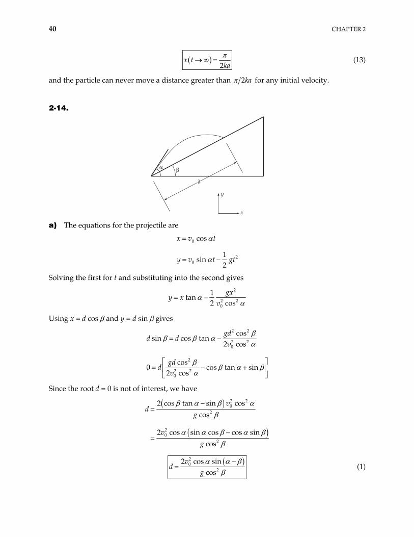
2-14.
y
x
d
! "
a) The equations for the projectile are
0
20
cos
1sin
2
x v t
y v t gt
Solving the first for t and substituting into the second gives
2
2 20
1tan
2 cosgx
y xv
Using x = d cos and y = d sin gives
2 2
2 20
2
2 20
cossin cos tan
2 cos
cos0 cos tan
2 cos
gdd d
v
gdd
vsin
Since the root d = 0 is not of interest, we have
2 20
2
20
2
2 cos tan sin coscos
2 cos sin cos cos sincos
vd
g
vg
20
2
2 cos sincos
vd
g (1)
NEWTONIAN MECHANICS—SINGLE PARTICLE 41
b) Maximize d with respect to
202
20 sin sin cos cos cos 2
cosvd
dd g
cos 2 0
22
4 2
c) Substitute (2) into (1)
20
max 2
2cos sin
cos 4 2 4 2v
gd
Using the identity
1 1
n sin 2 cos sin2 2
si A B A B A B
we have
2 20 0
max 2 2
sin sin 1 sin2 2cos 2 1 sin
v vg g
d
20
max 1 sinv
dg
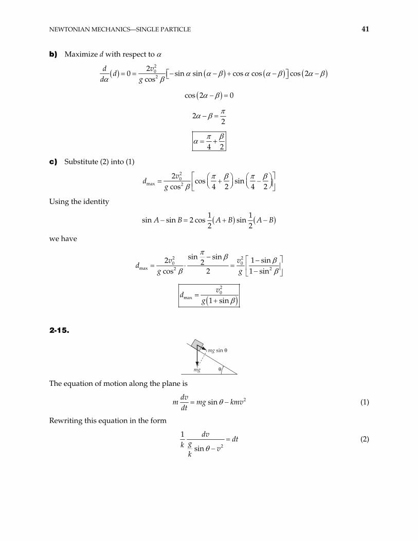
2-15.
mg #
mg sin #
The equation of motion along the plane is
2sindv
m mg kmdt
v (1)
Rewriting this equation in the form
2
1
sin
dvdtgk v
k
(2)
42 CHAPTER 2
We know that the velocity of the particle continues to increase with time (i.e., 0dv dt ), so that 2sing k v . Therefore, we must use Eq. (E.5a), Appendix E, to perform the integration. We
find
11 1tanh
sin sin
vt C
k g gk k
(3)
The initial condition v(t = 0) = 0 implies C = 0. Therefore,
sin tanh sing dx
v gkk d
tt
(4)
We can integrate this equation to obtain the displacement x as a function of time:
sin tanh sing
x gkk
t dt
Using Eq. (E.17a), Appendix E, we obtain
ln cosh sin
sinsin
gk tgk gk
x C (5)
The initial condition x(t = 0) = 0 implies C = 0. Therefore, the relation between d and t is
1
ln cosh sind gkk
t (6)
From this equation, we can easily find
1cosh
sin
dket
gk (7)
2-16. The only force which is applied to the article is the component of the gravitational force along the slope: mg sin . So the acceleration is g sin . Therefore the velocity and displacement along the slope for upward motion are described by:
0 sinv v g t (1)
20
1sin
2x v t g t (2)
where the initial conditions 00 vv t and 0x t 0 have been used.
At the highest position the velocity becomes zero, so the time required to reach the highest position is, from (1),
00 sin
vt
g (3)
At that time, the displacement is
NEWTONIAN MECHANICS—SINGLE PARTICLE 43
20
012 sin
vx
g (4)
For downward motion, the velocity and the displacement are described by
sinv g t (5)
21sin
2x g t (6)
where we take a new origin for x and t at the highest position so that the initial conditions are v(t = 0) = 0 and x(t = 0) = 0.
We find the time required to move from the highest position to the starting position by substituting (4) into (6):
0
sinv
tg
(7)
Adding (3) and (7), we find
02sinv
tg
(8)
for the total time required to return to the initial position.
2-17.
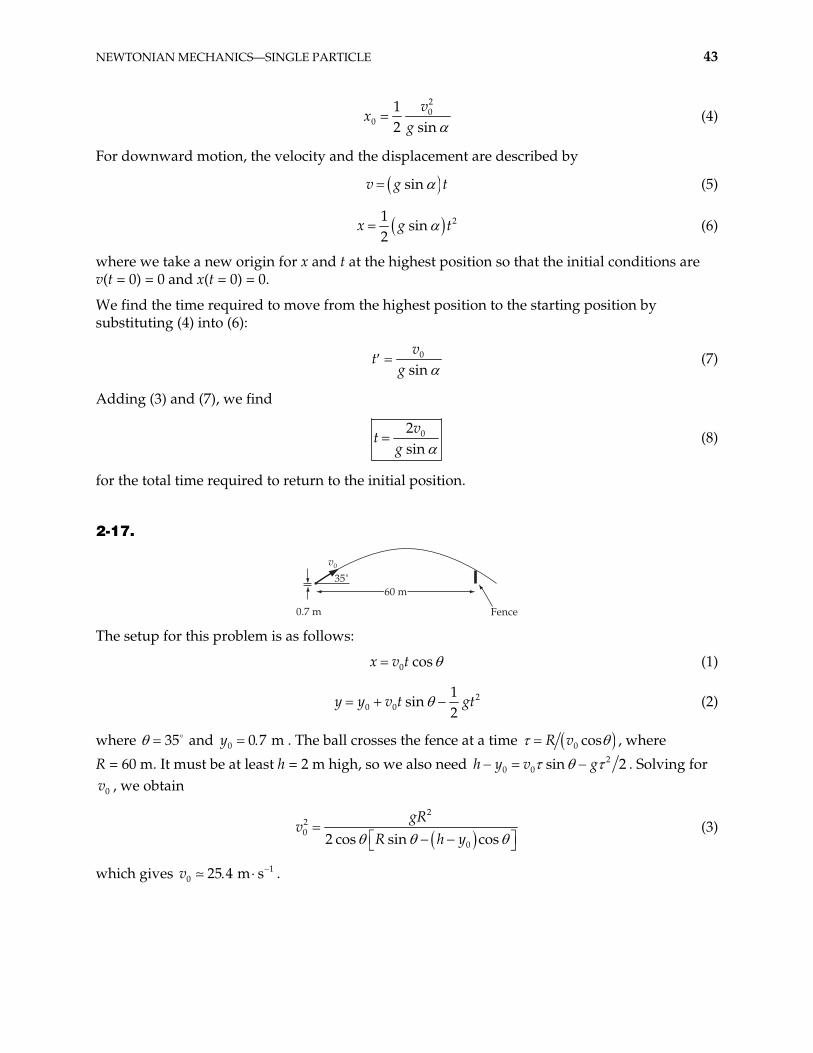
v0
Fence
35˚
0.7 m
60 m
The setup for this problem is as follows:
0 cosx v t (1)
20 0
1sin
2y y v t gt (2)
where and . The ball crosses the fence at a time 35 0 0 7 my 0 cosR v , where
R = 60 m. It must be at least h = 2 m high, so we also need 20 0 sinv g 2h y . Solving for
, we obtain 0v
2
20
02 cos sin cosgR
vR h y
(3)
which gives v . 10 25 4 m s
44 CHAPTER 2
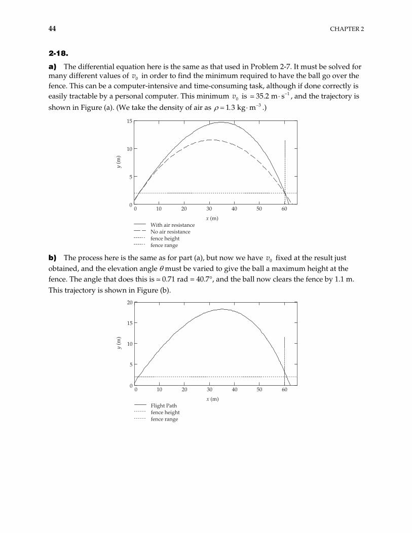
2-18.
a) The differential equation here is the same as that used in Problem 2-7. It must be solved for many different values of v in order to find the minimum required to have the ball go over the fence. This can be a computer-intensive and time-consuming task, although if done correctly is easily tractable by a personal computer. This minimum is
0
0v 135.2 m s3m
, and the trajectory is shown in Figure (a). (We take the density of air as 1 3 kg .)
0 10 20 30 40 50 600
5
10
15
With air resistanceNo air resistancefence heightfence range
x (m)
y (m
)
b) The process here is the same as for part (a), but now we have v fixed at the result just obtained, and the elevation angle must be varied to give the ball a maximum height at the fence. The angle that does this is 0.71 rad = 40.7°, and the ball now clears the fence by 1.1 m. This trajectory is shown in Figure (b).
0
0 10 20 30 40 50 600
5
10
15
20
Flight Pathfence heightfence range
x (m)
y (m
)
NEWTONIAN MECHANICS—SINGLE PARTICLE 45
2-19. The projectile’s motion is described by
0
20
cos
1sin
2
x v t
y v t gt (1)
where v is the initial velocity. The distance from the point of projection is 0
2r x y2 (2)
Since r must always increase with time, we must have : 0r
0xx yy
rr
(3)
Using (1), we have
2 3 2 20
1 3sin
2 2yy g t g v t v t0xx (4)
Let us now find the value of t which yields 0xx yy (i.e., 0r ):
20 0sin39 sin 8
2 2v v
tg g
(5)
For small values of , the second term in (5) is imaginary. That is, r = 0 is never attained and the value of t resulting from the condition 0r is unphysical.
Only for values of greater than the value for which the radicand is zero does t become a physical time at which does in fact vanish. Therefore, the maximum value of that insures
for all values of t is obtained from r
0r
2max9 sin 8 0 (6)
or,
max2 2
sin3
(7)
so that
max 70.5 (8)
2-20. If there were no retardation, the range of the projectile would be given by Eq. (2.54):
20
0sin 2v
Rg
(1)
The angle of elevation is therefore obtained from
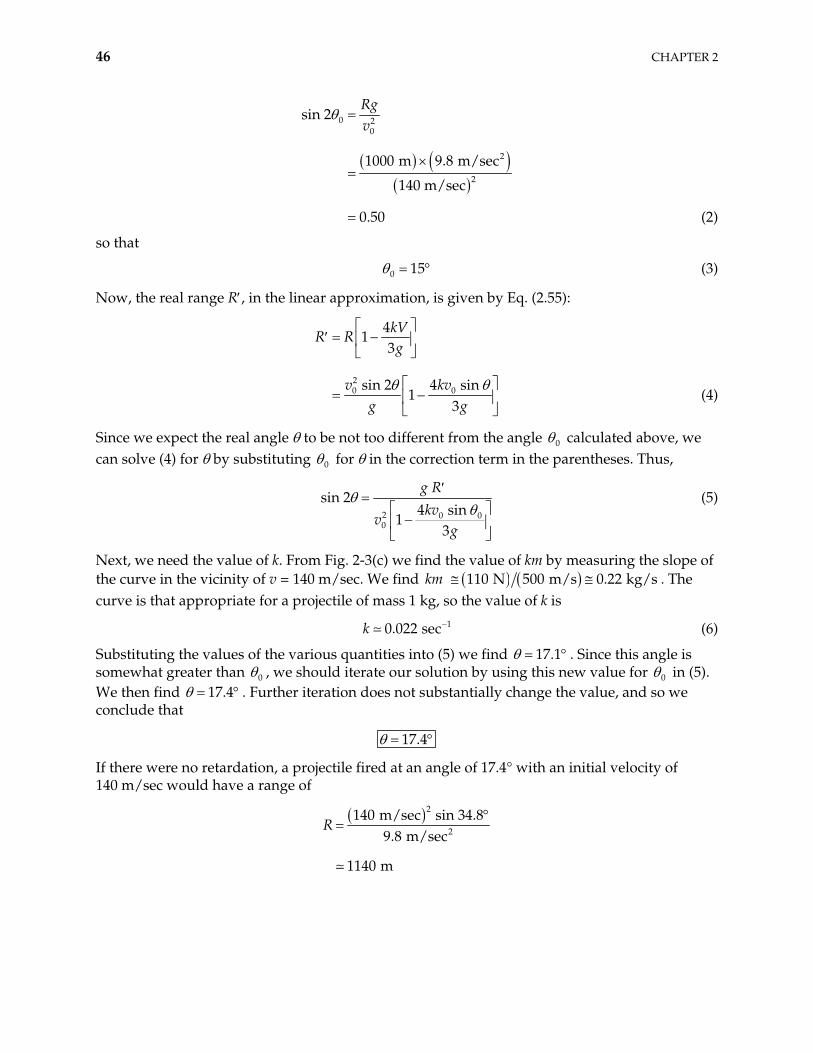
46 CHAPTER 2
0 20
2
2
sin 2
1000 m 9.8 m/sec
140 m/sec
0.50
Rgv
(2)
so that
0 15 (3)
Now, the real range R , in the linear approximation, is given by Eq. (2.55):
20 0
41
3
sin 2 4 sin1
3
kVR R
g
v kvg g
(4)
Since we expect the real angle to be not too different from the angle 0 calculated above, we can solve (4) for by substituting 0 for in the correction term in the parentheses. Thus,
2 0 00
sin 24 sin
13
g Rkv
vg
(5)
Next, we need the value of k. From Fig. 2-3(c) we find the value of km by measuring the slope of the curve in the vicinity of v = 140 m/sec. We find 110 N 500 m/s 0.22 kg/skm . The curve is that appropriate for a projectile of mass 1 kg, so the value of k is
10.022 seck (6)
Substituting the values of the various quantities into (5) we find 17.1 . Since this angle is somewhat greater than 0 , we should iterate our solution by using this new value for 0 in (5). We then find 17.4 . Further iteration does not substantially change the value, and so we conclude that
17.4
If there were no retardation, a projectile fired at an angle of 17.4° with an initial velocity of 140 m/sec would have a range of
2
2
140 m/sec sin 34.89.8 m/sec
1140 m
R
NEWTONIAN MECHANICS—SINGLE PARTICLE 47
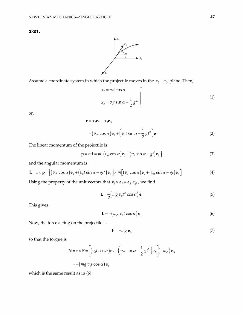
2-21.
x3
!
v0
x2
x1 Assume a coordinate system in which the projectile moves in the 2x x3 plane. Then,
2 0
23 0
cos
1sin
2
x v t
x v t gt (1)
or,
2 2 3 3
20 2 0
1cos sin
2
x x
v t v t gt
r e e
e 3e (2)
The linear momentum of the projectile is
0 2 0cos sinm m v v gt 3e ep r (3)
and the angular momentum is
20 2 0 3 0 2 0cos sin cos sinv t v t gt m v v gt 3L r p e e e e (4)
Using the property of the unit vectors that 3i j ijke e e , we find
20
1cos
2mg v tL 1e (5)
This gives
0 cosmg v tL 1e (6)
Now, the force acting on the projectile is
3mgF e (7)
so that the torque is
20 2 0 3
0 1
1cos sin
2
cos
v t v t gt mg
mg v t
N r F e e e
e
3
which is the same result as in (6).
48 CHAPTER 2
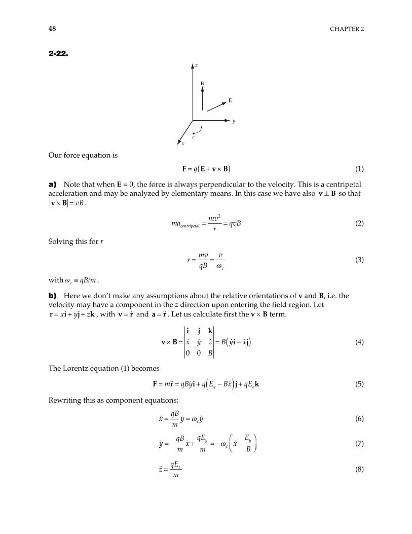
2-22.
x
y
z
e
B
E
Our force equation is
qF E v B (1)
a) Note that when E = 0, the force is always perpendicular to the velocity. This is a centripetal acceleration and may be analyzed by elementary means. In this case we have also so that v B
vBv B .
2
centripetalmv
ma qvBr
(2)
Solving this for r
c
mv vr
qB (3)
with c qB m .
b) Here we don’t make any assumptions about the relative orientations of v and B, i.e. the velocity may have a component in the z direction upon entering the field region. Let
, with x y zr i j k v r and . Let us calculate first the v B term. a r
0 0x y z B y x
B
i j kv B i j (4)
The Lorentz equation (1) becomes
y zm qBy q E Bx qEF r i j k (5)
Rewriting this as component equations:
cqB
x ym
y (6)
yc
qE EqBy x x
m m By (7)
zqEz
m (8)
NEWTONIAN MECHANICS—SINGLE PARTICLE 49
The z-component equation of motion (8) is easily integrable, with the constants of integration given by the initial conditions in the problem statement.
20 0 2
zqEz t z z t t
m (9)
c) We are asked to find expressions for and , which we will call and x y xv yv , respectively. Differentiate (6) once with respect to time, and substitute (7) for yv
2 yx c y c x
Ev v v
B (10)
or
2 2 yx c x c
Ev v
B (11)
This is an inhomogeneous differential equation that has both a homogeneous solution (the solution for the above equation with the right side set to zero) and a particular solution. The most general solution is the sum of both, which in this case is
1 2cos sin yx c c
Ev C t C t
B (12)
where C and C are constants of integration. This result may be substituted into (7) to get 1 2 yv
1 2cos siny c c cC t Cv ct (13)
1 2sin cosy c cv C t C t K (14)
where K is yet another constant of integration. It is found upon substitution into (6), however, that we must have K = 0. To compute the time averages, note that both sine and cosine have an average of zero over one of their periods 2 cT .
0yEx y
B (15)
d) We get the parametric equations by simply integrating the velocity equations.
1 2sin cos yc c
c c
EC Ct
B xt Dx t (16)
1 2cos sinc c yc c
C Cy t t D (17)
where, indeed, D and x yD are constants of integration. We may now evaluate all the C’s and
D’s using our initial conditions 0 cx A , 0 yx E B , 0 0y , 0y A . This gives us , and gives the correct answer 1 x yC D D 0 2C A
cos yc
c
EAx t t t
B (18)
50 CHAPTER 2
( ) sin cc
Ay t t (19)
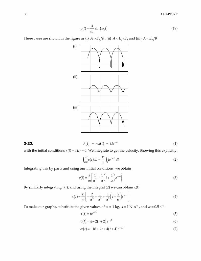
These cases are shown in the figure as (i) yA E B , (ii) yA E B , and (iii) yA E B .
(i)
(ii)
(iii)
2-23. atF t ma t kte (1)
with the initial conditions x(t) = v(t) = 0. We integrate to get the velocity. Showing this explicitly,
( )
(0) 0
v t t t
v
ka t dt te dt
m (2)
Integrating this by parts and using our initial conditions, we obtain
2
1 1 1( ) tk
v t t em
(3)
By similarly integrating v(t), and using the integral (2) we can obtain x(t).
3 2 2
2 1 1 2 tkx t t e
m (4)
To make our graphs, substitute the given values of m = 1 kg, 11 N sk , and . 10.5 s
2tx t te (5)
24 2 2 tv t t e (6)
216 4 4 4 tt t t e (7)
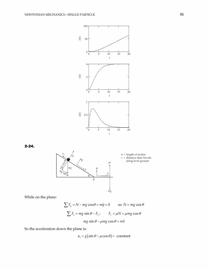
NEWTONIAN MECHANICS—SINGLE PARTICLE 51
0 5 10 15 200
50
100
t
x(t)
0 5 10 15 200
2
4
t
v(t)
0 5 10 15 200
0.5
1
t
a(t)
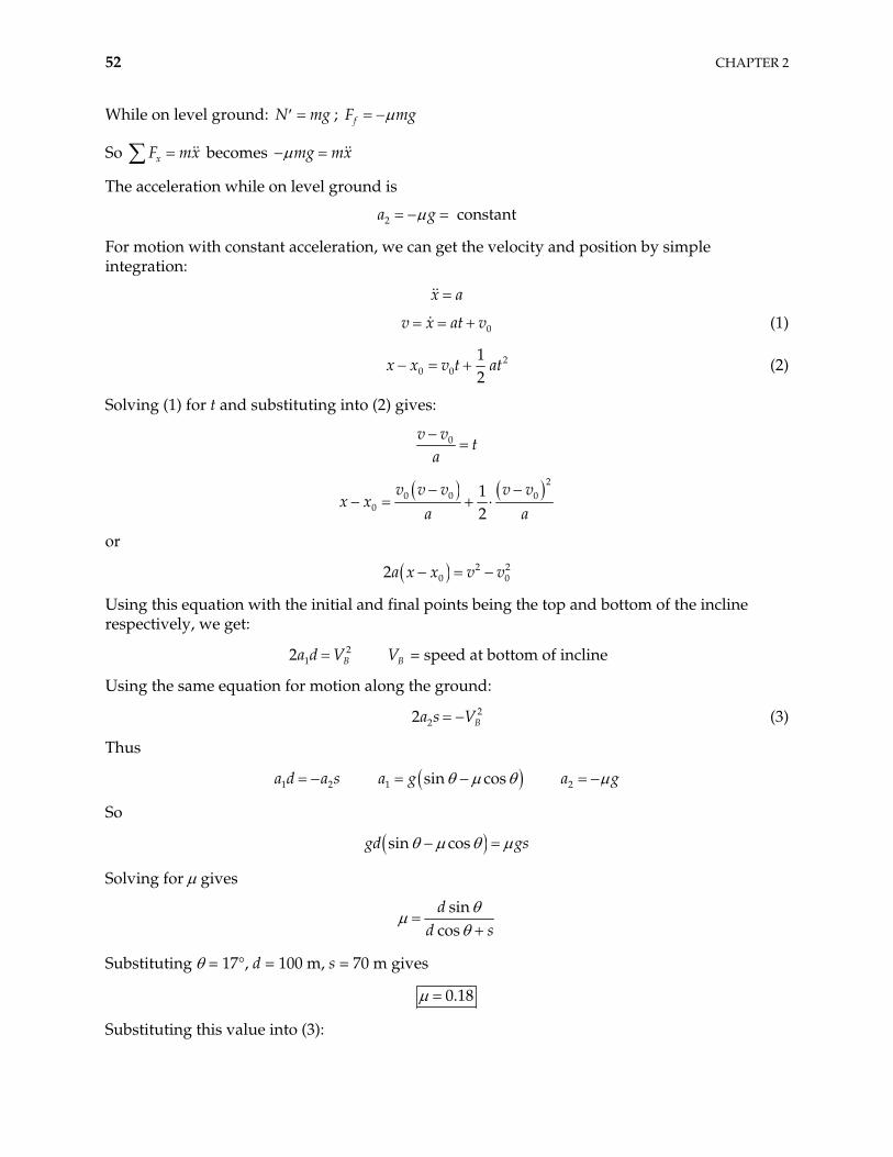
2-24.
mg
mg
Ff
Ff N
B
N$
d = length of inclines = distance skier travels
along level ground
# x
mg sin #
mg
cos #
y
y
x
While on the plane:
F N so N mcos 0y mg my cosg
sinx fF m ; g F cosfF N mg
sin cosmg mg mx
So the acceleration down the plane is:
1 sin cos constanta g
52 CHAPTER 2
While on level ground: ; N mg gfF m
So becomes xF mx mg mx
The acceleration while on level ground is
2 constanta g
For motion with constant acceleration, we can get the velocity and position by simple integration:
x a
0v x at v (1)
20 0
12
x x v t at (2)
Solving (1) for t and substituting into (2) gives:
0v vt
a
2
0 0 00
12
v v v v vx x
a a
or
2 20 02a x x v v
Using this equation with the initial and final points being the top and bottom of the incline respectively, we get:
2 = speed at bottom of incline 21 Ba d V BV
Using the same equation for motion along the ground:
222 Ba s V (3)
Thus
a d 1 a s2 1 sin cosa g 2a g
So
sin cosgd gs
Solving for gives
sin
cosd
d s
Substituting = 17°, d = 100 m, s = 70 m gives
0.18
Substituting this value into (3):
NEWTONIAN MECHANICS—SINGLE PARTICLE 53
22 Bgs V
2BV gs
15.6 m/secBV
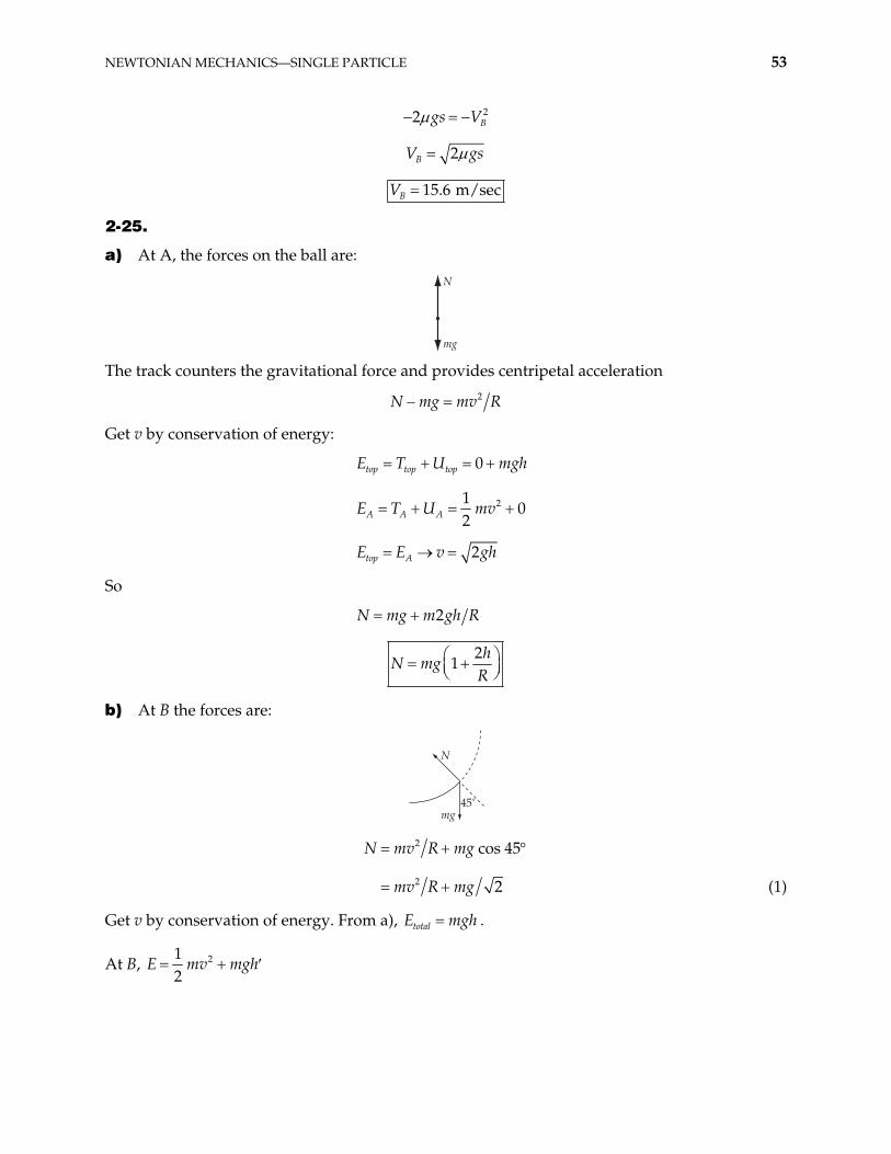
2-25.
a) At A, the forces on the ball are:
N
mg The track counters the gravitational force and provides centripetal acceleration
2N mg mv R
Get v by conservation of energy:
0top top topE T U mgh
210
2A A AE T U mv
2top AE E v gh
So
2N mg m gh R
2
1h
N mgR
b) At B the forces are:
mg
N
45˚
2
2
cos 45
2
N mv R mg
mv R mg (1)
Get v by conservation of energy. From a), totalE mgh .
At B, 212
v mghE m
54 CHAPTER 2
RR
h$45˚
R Rcos 45 2˚ =
R 2
2
RR h or
11
2h R
So becomes: total B BE T U
21 11
22mgh mgR mv
Solving for 2v
212 1
2gh gR v
Substituting into (1):
2 3
22
hN mg
R
c) From b) 2 2 2B h R Rv g
1 2
2 2v g h R R
d) This is a projectile motion problem
45˚
45˚B
A Put the origin at A.
The equations:
0 0xx x v t
20 0
12yy y v t gt
become
2 2
BvRx t (2)
2122
Bvy h t gt (3)
Solve (3) for t when y = 0 (ball lands).
NEWTONIAN MECHANICS—SINGLE PARTICLE 55
2 2 2Bgt v t h 0
22 2 8
2B Bv v g
tg
h
We discard the negative root since it gives a negative time. Substituting into (2):
22 2 8
22 2B BB v v ghvR
xg
Using the previous expressions for and h yields Bv
1 2
2 2 232 1 2
2h h R Rx R
e) , with , so U x has the shape of the track. ( ) ( )U x mgy x (0)y h ( )
2-26. All of the kinetic energy of the block goes into compressing the spring, so that 2 22 2mv kx , or 2 3 mx v m k , where x is the maximum compression and the given
values have been substituted. When there is a rough floor, it exerts a force kmg in a direction that opposes the block’s velocity. It therefore does an amount of work kmgd in slowing the block down after traveling across the floor a distance d. After 2 m of floor, the block has energy
2 2 kmv mgd , which now goes into compressing the spring and still overcoming the friction
on the floor, which is 2 2 kkx mgx . Use of the quadratic formula gives
2 2 2mg mg mgdmv
k k k kx (1)
Upon substitution of the given values, the result is 1.12 m.
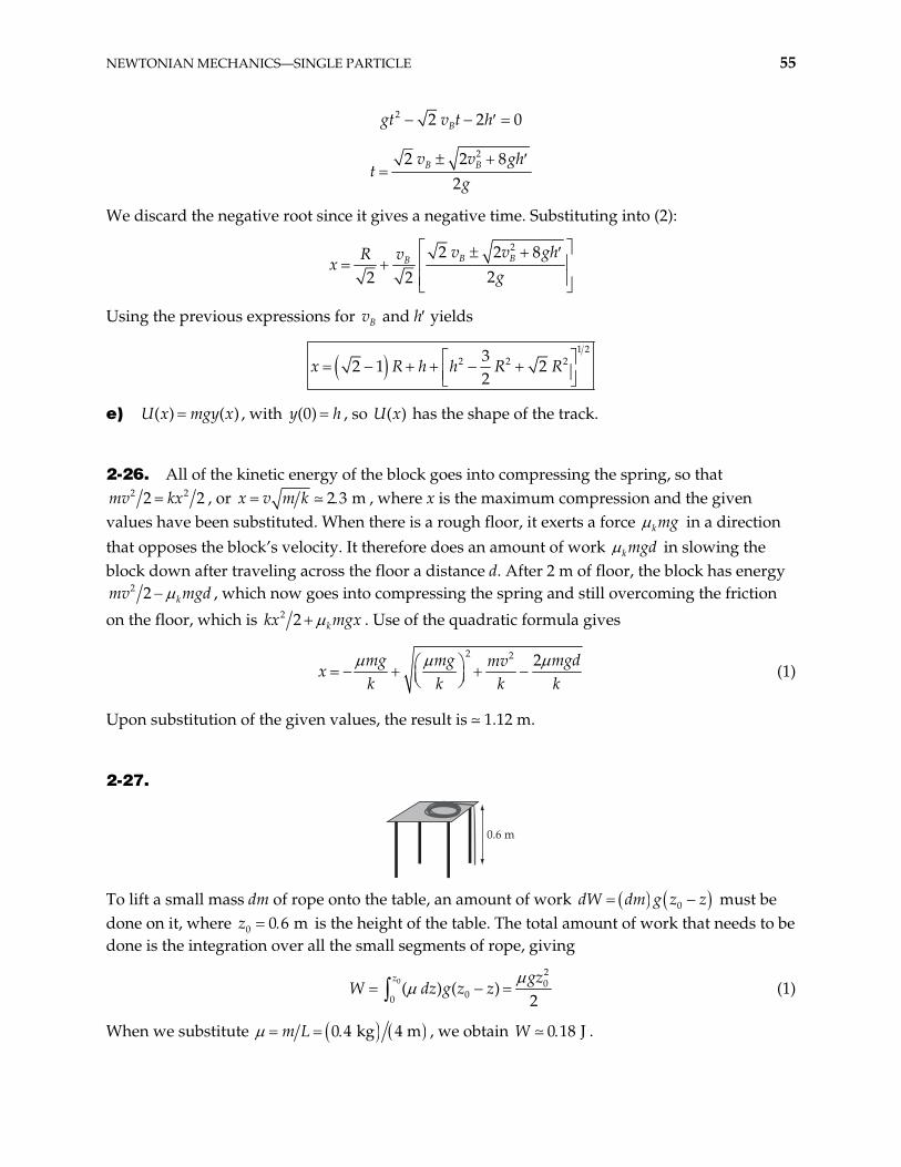
2-27.
0.6 m
To lift a small mass dm of rope onto the table, an amount of work 0dW dm g z z must be done on it, where 0 0 6 mz is the height of the table. The total amount of work that needs to be done is the integration over all the small segments of rope, giving
020
00( ) ( )
2z gz
W dz g z z (1)
When we substitute 0 4 kg 4 mm L , we obtain 0 18 JW .
56 CHAPTER 2
2-28.
m
M
v
v
v4
v3
beforecollision
aftercollision
The problem, as stated, is completely one-dimensional. We may therefore use the elementary result obtained from the use of our conservation theorems: energy (since the collision is elastic) and momentum. We can factor the momentum conservation equation
1 1 2 2 1 3 2 4m v m v m v m v (1)
out of the energy conservation equation
2 2 21 1 2 2 1 3 2 4
1 1 1 12 2 2 2
m v m v m v m v2
4
(2)
and get
1 3 2v v v v (3)
This is the “conservation” of relative velocities that motivates the definition of the coefficient of restitution. In this problem, we initially have the superball of mass M coming up from the ground with velocity 2gv , while the marble of mass m is falling at the same velocity. Conservation of momentum gives
h
3 4Mv m v Mv mv (4)
and our result for elastic collisions in one dimension gives
3 ( )v v v v4 (5)
solving for and and setting them equal to 3v 4v 2 itemgh , we obtain
23
1marbleh h (6)
21 3
1superballh h (7)
where m M . Note that if 1 3 , the superball will bounce on the floor a second time after the collision.
NEWTONIAN MECHANICS—SINGLE PARTICLE 57
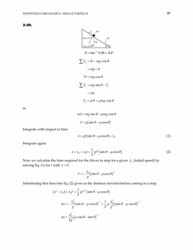
2-29.
mg cos #
mg sin #
mg
Ff N
y
x#
1tan 0.08 4.6
cos
0
cos
sin
cos
y
x f
f
F N mg
my
N mg
F mg F
mx
F N mg
so
sin cos
sin cos
mx mg mg
x g
Integrate with respect to time
0sin cosx gt x (1)
Integrate again:
20 0
1sin cos
2x x x t gt (2)
Now we calculate the time required for the driver to stop for a given (initial speed) by solving Eq. (1) for t with .
0x0x
10 sin cos
xt
g
Substituting this time into Eq. (2) gives us the distance traveled before coming to a stop.
20 0
2 21 10 0
2
210
1sin cos
2
1sin cos sin cos
2
cos sin2
x x x t gt
x xx g
g g
xx
g
58 CHAPTER 2
We have 4.6 , 0.45 , . 29.8 m/secg
For , . 0 25 mph 11.2 m/secx 17.4 metersx
If the driver had been going at 25 mph, he could only have skidded 17.4 meters.
Therefore, he was speeding
How fast was he going?
gives . 30 metersx 0 32.9 mphx
2-30. 1T t t2 (1)
where T = total time = 4.021 sec.
= the time required for the balloon to reach the ground. 1t
= the additional time required for the sound of the splash to reach the first student.
2t
We can get t from the equation 1
20 0
12
y y y t gt ; 0 0 0y y
When , y = –h; so (h = height of building) 1t t
21
12
h gt or 12hg
t
distance sound travels
speed of soundhv
t
Substituting into (1):
2h hg v
T or 2
0h h
Tv g
This is a quadratic equation in the variable h . Using the quadratic formula, we get:
2 2 42
1 12 2
Tg g v gTv
Vgv
h
Substituting 331 m/secV
29.8 m/secg
4.021 secT
and taking the positive root because it is the physically acceptable one, we get:
NEWTONIAN MECHANICS—SINGLE PARTICLE 59
1 28.426 mh
h = 71 meters
2-31. For , example 2.10 proceeds as is until the equations following Eq. (2.78). Proceeding from there we have
0 0x
0 0B x
0A z
so
0 00 cos sin
z xx x t t
0 0y y y t
0 00 cos sin
x zz z t t
Note that
2 2
2 2 0 00 0 2 2
z xx x z z
Thus the projection of the motion onto the x–z plane is a circle of radius 1 22 2
0 01
x z .
1 22 20 0
0
So the motion is unchanged except for a change in the
the helix. The new radius is .m
x zqB
radius of
2-32.
The forces on the hanging mass are
T
mg The equation of motion is (calling downward positive)
mg T ma or T m g a (1)
The forces on the other mass are
60 CHAPTER 2
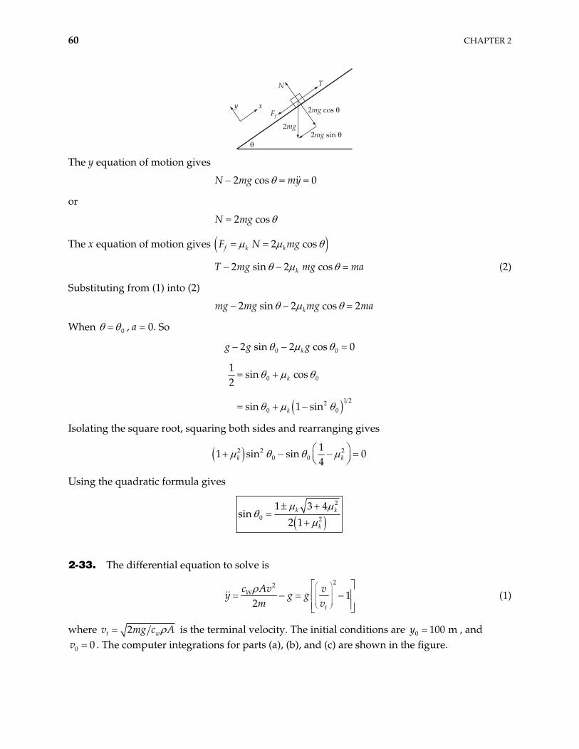
y xFf
N T
#
2mg
2mg cos #
2mg sin #
The y equation of motion gives
2 cosN mg my 0
or
2 cosN mg
The x equation of motion gives 2 cosf k kF N mg
2 sin 2 coskT mg mg ma (2)
Substituting from (1) into (2)
2 sin 2 cos 2kmg mg mg ma
When 0 , a = 0. So
0 02 sin 2 cos 0kg g g
0 0
1 220 0
1sin cos
2
sin 1 sin
k
k
Isolating the square root, squaring both sides and rearranging gives
2 2 20 0
11 sin sin
4k k 0
Using the quadratic formula gives
2
0 2
1 3 4sin
2 1k k
k
2-33. The differential equation to solve is
22
12
W
t
c Av vy g g
m v (1)
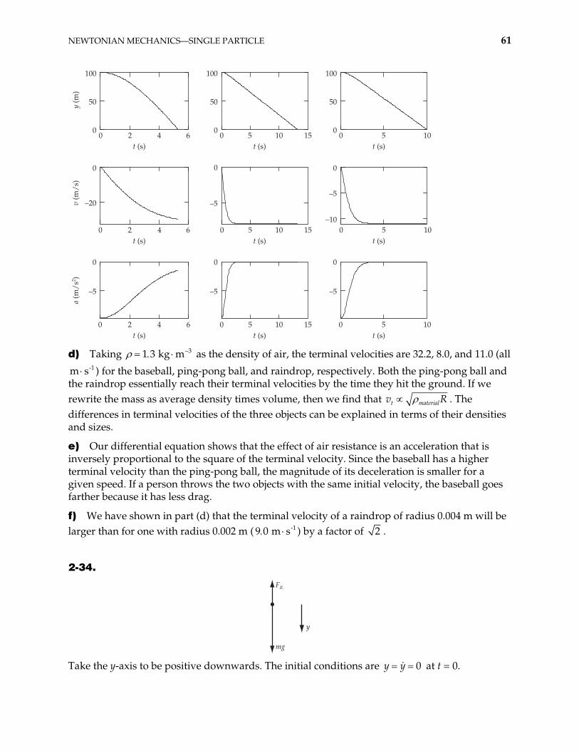
where 2t g cw Av m is the terminal velocity. The initial conditions are , and . The computer integrations for parts (a), (b), and (c) are shown in the figure.
0 100 my
0 0v
NEWTONIAN MECHANICS—SINGLE PARTICLE 61
0 50
50
100
10t (s)
0 5–10
–5
0
10t (s)
0 5
–5
0
10t (s)
0 2 4 60
50
100
t (s)
y (m
)
0 2 4 6
–20
0
t (s)
v (m
/s)
0 2 4 6
–5
0
t (s)
a (m
/s2 )
0 5 10 150
50
100
t (s)
0 5 10 15
–5
0
t (s)
0 5 10 15
–5
0
t (s)
d) Taking as the density of air, the terminal velocities are 32.2, 8.0, and 11.0 (all
) for the baseball, ping-pong ball, and raindrop, respectively. Both the ping-pong ball and the raindrop essentially reach their terminal velocities by the time they hit the ground. If we rewrite the mass as average density times volume, then we find that
31 3 kg m-1m s
t materialv R . The differences in terminal velocities of the three objects can be explained in terms of their densities and sizes.
e) Our differential equation shows that the effect of air resistance is an acceleration that is inversely proportional to the square of the terminal velocity. Since the baseball has a higher terminal velocity than the ping-pong ball, the magnitude of its deceleration is smaller for a given speed. If a person throws the two objects with the same initial velocity, the baseball goes farther because it has less drag.
f) We have shown in part (d) that the terminal velocity of a raindrop of radius 0.004 m will be larger than for one with radius 0.002 m ( -19 0 m s ) by a factor of 2 .
2-34.
FR
y
mg Take the y-axis to be positive downwards. The initial conditions are 0y y at t = 0.
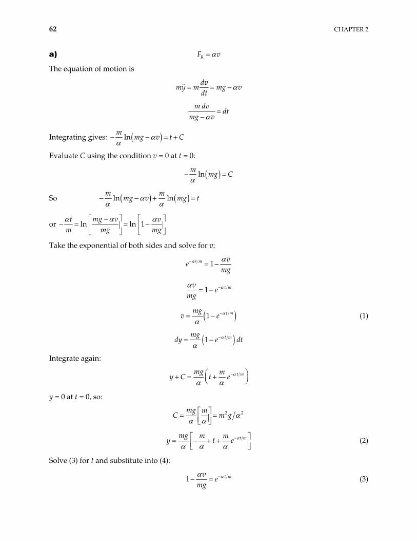
62 CHAPTER 2
a) RF v
The equation of motion is
dv
my m mg vdt
m dv
dtmg v
Integrating gives: lnm
mg v t C
Evaluate C using the condition v = 0 at t = 0:
lnm
mg C
So ln lnm m
mg v mg t
or ln ln 1mg vt v
m mg
mg
Take the exponential of both sides and solve for v:
1r m ve
mg
1 t mve
mg
1 t mmgv e (1)
1 t mmgdy e dt
Integrate again:
t mmg my C t e
y = 0 at t = 0, so:
2 2mg mC m g
t mmg m my t e (2)
Solve (3) for t and substitute into (4):
1 t mve
mg (3)
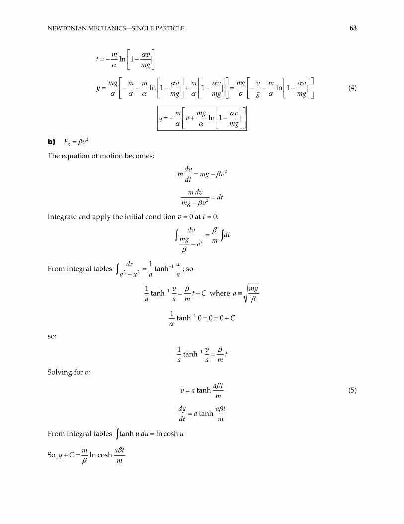
NEWTONIAN MECHANICS—SINGLE PARTICLE 63
ln 1m v
tmg
ln 1 1 ln 1mg mgm m v m v v m v
ymg mg g mg
(4)
ln 1mgm v
y vmg
b) 2RF v
The equation of motion becomes:
2dvm mg
dtv
2
m dvdt
mg v
Integrate and apply the initial condition v = 0 at t = 0:
2
dvdtmg mv
From integral tables 12 2
1tanh
dx xa x a a
; so
11tanh
vt C
a a m where
mga
11tanh 0 0 0 C
so:
11tanh
vt
a a m
Solving for v:
tanha t
v am
(5)
tanhdy a t
adt m
From integral tables tanh ln coshu du u
So ln coshm a
y Cm
t
64 CHAPTER 2
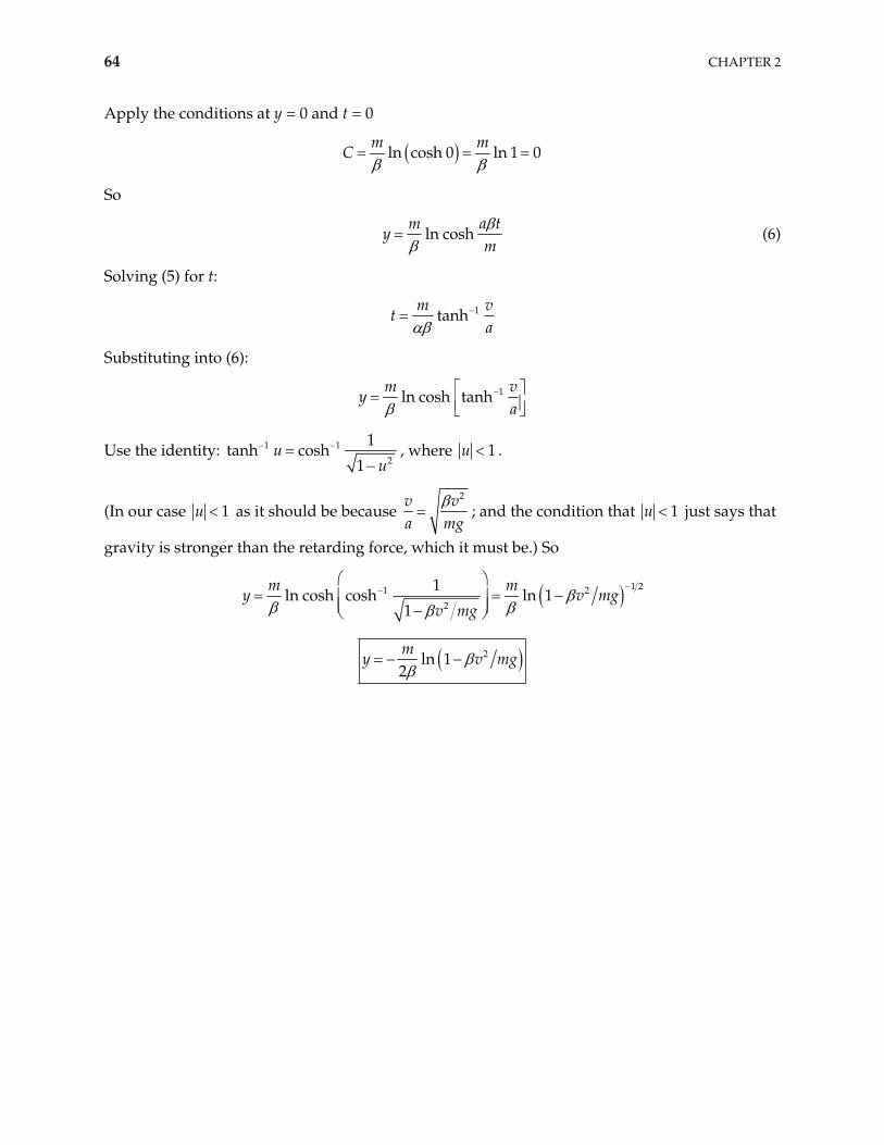
Apply the conditions at y = 0 and t = 0
ln cosh 0 ln 1 0m m
C
So
ln coshm a
ym
t (6)
Solving (5) for t:
1tanhm v
ta
Substituting into (6):
1ln cosh tanhm v
ya
Use the identity: 1 1
2
1tanh cosh
1u
u, where 1u .
(In our case 1u as it should be because 2v v
a mg; and the condition that 1u just says that
gravity is stronger than the retarding force, which it must be.) So
1 21 2
2
1ln cosh cosh ln 1
1
m m
v mgy v mg
2ln 12m
y v mg
NEWTONIAN MECHANICS—SINGLE PARTICLE 65
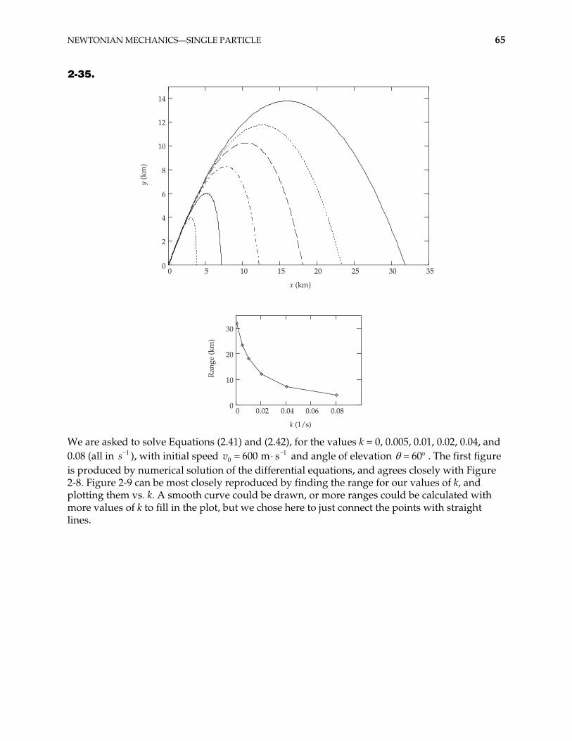
2-35.
0 5 10 15 20 25 30 350
2
4
6
8
10
12
14
x (km)
y (k
m)
0 0.02 0.04 0.06 0.080
10
20
30
k (1/s)
Ran
ge (k
m)
We are asked to solve Equations (2.41) and (2.42), for the values k = 0, 0.005, 0.01, 0.02, 0.04, and 0.08 (all in ), with initial speed v1s 1
0 600 m s and angle of elevation 60 . The first figure is produced by numerical solution of the differential equations, and agrees closely with Figure 2-8. Figure 2-9 can be most closely reproduced by finding the range for our values of k, and plotting them vs. k. A smooth curve could be drawn, or more ranges could be calculated with more values of k to fill in the plot, but we chose here to just connect the points with straight lines.
66 CHAPTER 2
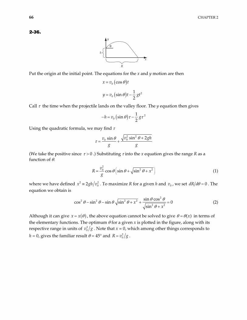
2-36.
#
h
y
x
R Put the origin at the initial point. The equations for the x and y motion are then
0 cosx v t
20
1sin
2y v t gt
Call the time when the projectile lands on the valley floor. The y equation then gives
20
1sin
2h v g
Using the quadratic formula, we may find
2 200 sin 2sin v gv
g gh
(We take the positive since 0 .) Substituting into the x equation gives the range R as a function of .
2
20 cos sin sinv
Rg
2x (1)
where we have defined 202x gh v2 . To maximize R for a given h and , we set 0v 0dR d . The
equation we obtain is
2
2 2 2 2
2 2
sin cosos sin sin sin 0
sinx
xc (2)
Although it can give x x , the above equation cannot be solved to give ( )x in terms of the elementary functions. The optimum for a given x is plotted in the figure, along with its respective range in units of 2
0v g . Note that x = 0, which among other things corresponds to
h = 0, gives the familiar result = 45° and 20R v g .
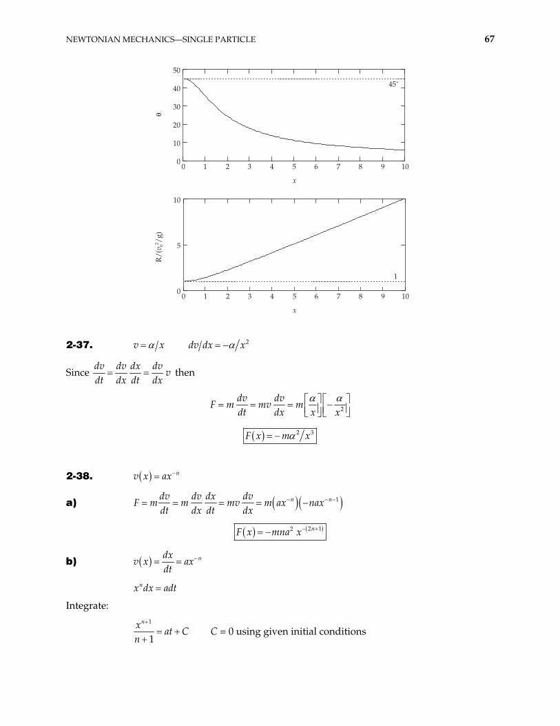
NEWTONIAN MECHANICS—SINGLE PARTICLE 67
0 1 2 3 4 5 6 7 8 90
10
20
30
40
50
10
x
#
0 1 2 3 4 5 6 7 8 90
5
10
10
x
R/(
v 02 /g
)
45˚
1
2-37. v x 2dv dx x
Since dv dv dx dv
vdt dx dt dx
then
2
dv dvF m mv m
dt dx x x
2 3F x m x
2-38. nv x ax
a) 1n ndv dv dx dvF m m mv m ax nax
dt dx dt dx
2 12 nF x mna x
b) ndxv x ax
dt
nx dx adt
Integrate:
1
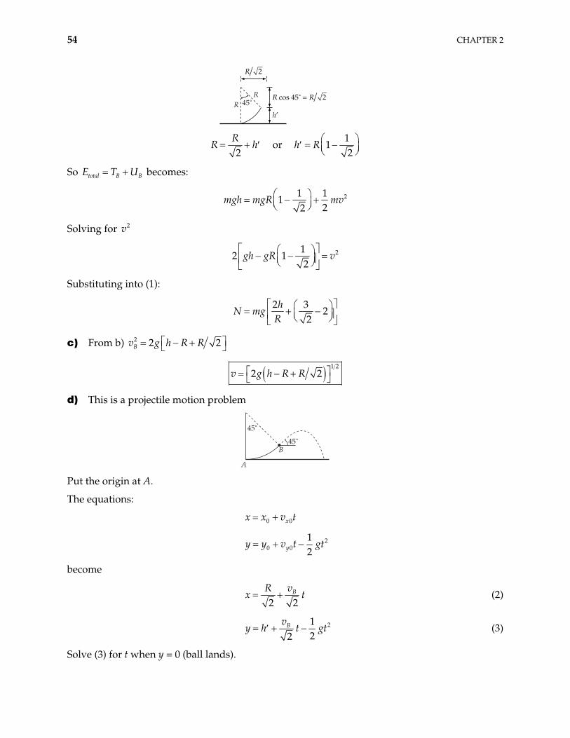
1
nxat C
n C = 0 using given initial conditions
68 CHAPTER 2
1 1nx n at
1 11 nx n at
c) Substitute x(t) into F(x):
2 11 12 1
nnF t mna n at
2 1 12 1 n nF t mna n at
2-39.
a) vF e
vdve
dt m
ve dv dm
t
1 ve t
mC
0v v at t = 0, so
01 ve C
01 vve e
mt
Solving for v gives
01
ln vtv t e
m
b) Solve for t when v = 0
0 1vte
m
01 vmt e
c) From a) we have
01
ln vtdx e dt
m
NEWTONIAN MECHANICS—SINGLE PARTICLE 69
Using ln lnax b
ax b dx ax b xa
we obtain
0 0ln1
v vt te em m t
mx C
Evaluating C using x = 0 at t = 0 gives
00 vv mC e
So
0 002 lnv vmv t m t t
e em m
0vx e
Substituting the time required to stop from b) gives the distance required to stop
00
1 1vmx e v
2-40.
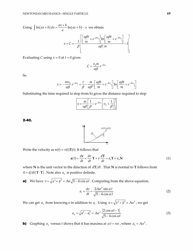
y
an at
(x(t),y(t))
x Write the velocity as v(t) = v(t)T(t). It follows that
t nd dv d
t v adt dt dtv T
a T T a N (1)
where N is the unit vector in the direction of d dT t . That N is normal to T follows from 0 d dt T T . Note also is positive definite. na
a) We have 22 5 4 cosyv Ax t . Computing from the above equation,
22 sin
5 4 costA tdv
adt t
(2)
We can get from knowing a in addition to . Using na ta 2 22 ya Ax , we get
2 2 2 2 cos 15 4 cosn t
ta a a A
t (3)
b) Graphing versus t shows that it has maxima at na t n , where 2na A .
70 CHAPTER 2
2-41.
a) As measured on the train:
0iT ; 212fT m v
212
T mv
b) As measured on the ground:
212iT mu ; 21
2fT m v u
212
T mv mvu
c) The woman does an amount of work equal to the kinetic energy gain of the ball as measured in her frame.
212
W mv
d) The train does work in order to keep moving at a constant speed u. (If the train did no work, its speed after the woman threw the ball would be slightly less than u, and the speed of the ball relative to the ground would not be u + v.) The term mvu is the work that must be supplied by the train.
W mvu
2-42.
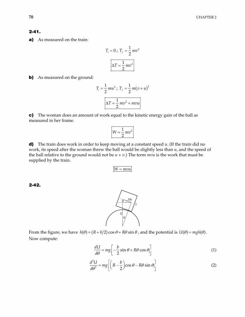
R##
#
b
R
From the figure, we have ( ) ( 2) cos sinh R b R , and the potential is U m( ) ( )gh . Now compute:
sin cos2
dU bmg R
d (1)
2
2 cos sin2
d U bmg R R
d (2)
NEWTONIAN MECHANICS—SINGLE PARTICLE 71
The equilibrium point (where 0ddU ) that we wish to look at is clearly = 0. At that point,
we have 2 2 2d U d mg R b , which is stable for 2R b and unstable for R b . We can
use the results of Problem 2-46 to obtain stability for the case
2
2R b , where we will find that the first non-trivial result is in fourth order and is negative. We therefore have an equilibrium at
= 0 which is stable for 2R b and unstable for 2R b .
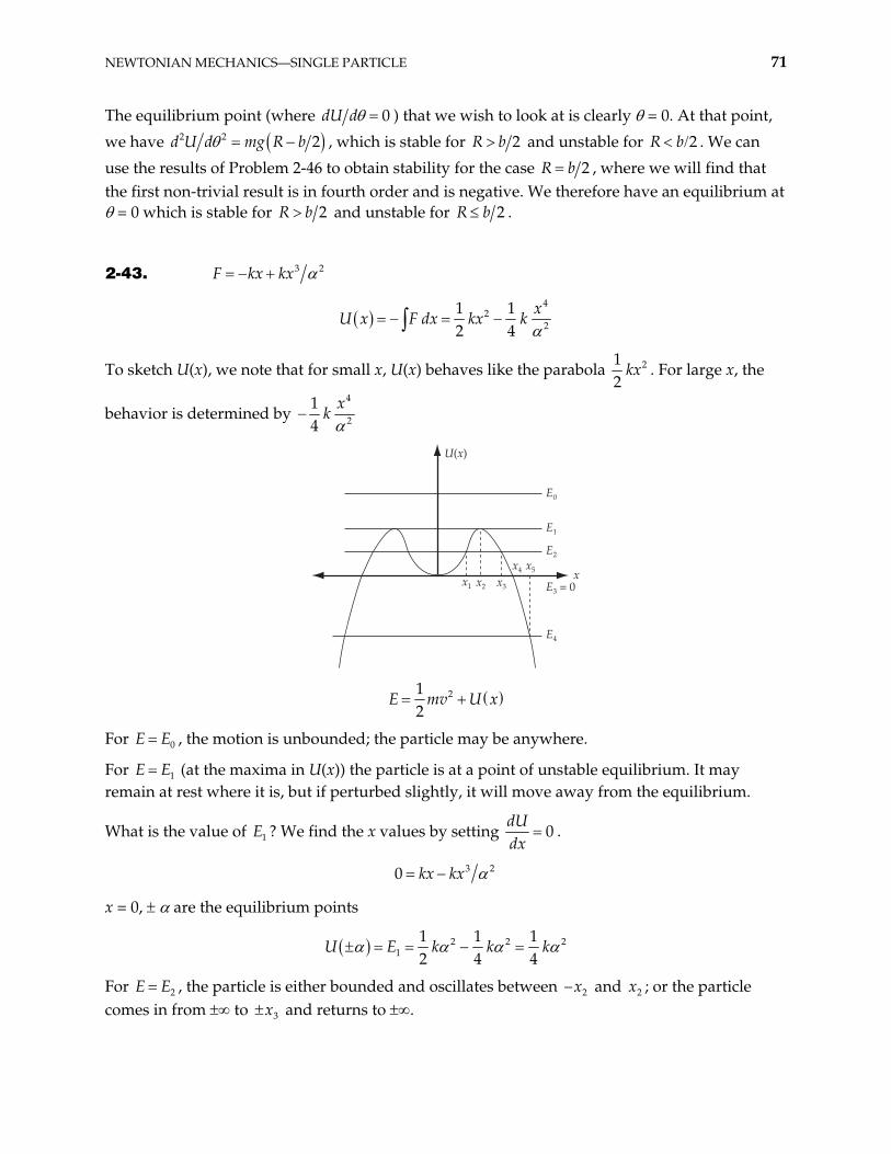
2-43. 3 2F kx kx
4
22
1 12 4
xU x F dx kx k
To sketch U(x), we note that for small x, U(x) behaves like the parabola 212
kx . For large x, the
behavior is determined by 4
2
14
xk
U(x)
E0
E1
E2
E3 = 0
E4
x1 x2 x3
x4 x5 x
212
E mv U x
For E , the motion is unbounded; the particle may be anywhere. 0E
For E (at the maxima in U(x)) the particle is at a point of unstable equilibrium. It may remain at rest where it is, but if perturbed slightly, it will move away from the equilibrium.
1E
What is the value of ? We find the x values by setting 1E 0dUdx
.
3 20 kx kx
x = 0, are the equilibrium points
2 21
1 1 12 4 4
U E k k k 2
For E , the particle is either bounded and oscillates between 2E 2x and ; or the particle comes in from to and returns to .
2x
3x
72 CHAPTER 2
For E , the particle is either at the stable equilibrium point x = 0, or beyond . 3 0 4x x
For E , the particle comes in from to 4 5x and returns.
2-44.
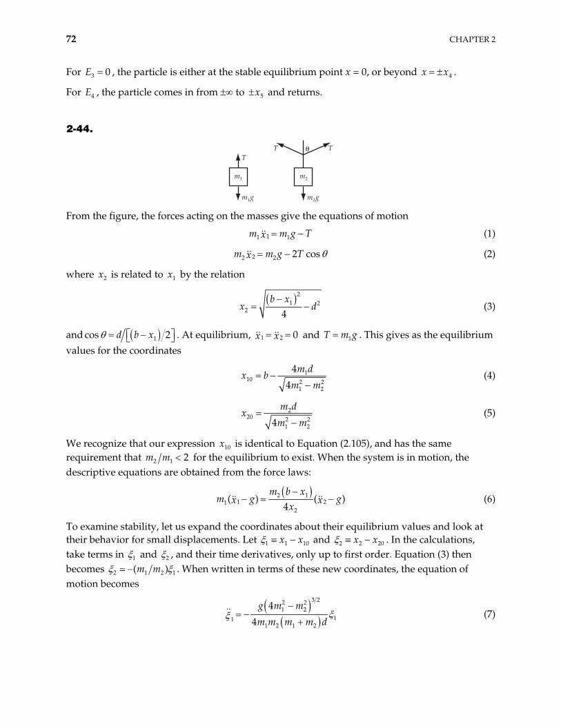
m1
T
m1g
m2
T T
m2g
#
From the figure, the forces acting on the masses give the equations of motion
11 1m m gx T (1)
22 2 2 cosm m g Tx (2)
where is related to by the relation 2x 1x
2
1 22 4
b xx d (3)
and 1cos 2d b x . At equilibrium, 1 2 0x x and T m1g . This gives as the equilibrium values for the coordinates
110 2
1 2
4
4
m dx b
m m2 (4)
220 2
1 24
m dx
m m2 (5)
We recognize that our expression is identical to Equation (2.105), and has the same requirement that
10x
2 1 2m m for the equilibrium to exist. When the system is in motion, the descriptive equations are obtained from the force laws:
2 111
2
( ) (4
m b xm gx
x 2 )gx
0
(6)
To examine stability, let us expand the coordinates about their equilibrium values and look at their behavior for small displacements. Let 1 1 1x x and 2 2 2x x 0 . In the calculations, take terms in 1 and 2 , and their time derivatives, only up to first order. Equation (3) then becomes 2 1 2(m m 1) . When written in terms of these new coordinates, the equation of motion becomes
3 22 2
1 211
1 2 1 2
4
4
g m m
m m m m d (7)
NEWTONIAN MECHANICS—SINGLE PARTICLE 73
which is the equation for simple harmonic motion. The equilibrium is therefore stable, when it exists.
2-45. and 2-46. Expand the potential about the equilibrium point
1 0
1!
ii
ii n
d uU x x
i dx (1)
The leading term in the force is then
( 1)
( 1)0
1( )
nn
n
dU d UF x x
dx n dx (2)
The force is restoring for a stable point, so we need 0F x 0 and 0F x 0 . This is never
true when n is even (e.g., U k ), and is only true for odd when 3x n ( 1) (n nd U dx 1)0
0 .
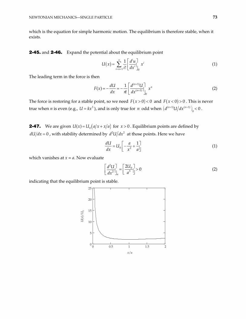
2-47. We are given 0( ) U a x x aU x for . Equilibrium points are defined by 0x
0dU dx , with stability determined by 2d U 2dx at those points. Here we have
0 2
1dU aU
dx x a (1)
which vanishes at x = a. Now evaluate
2
032
20
a
Ud Uadx
(2)
indicating that the equilibrium point is stable.
0 0.5 1 1.5 20
5
10
15
20
25
x/a
U(x
)/U
0
74 CHAPTER 2
2-48. In the equilibrium, the gravitational force and the eccentric force acting on each star must be equal
3 22 2
2
2/2 2
Gm mv mG d dv
d d d v mG
2-49. The distances from stars to the center of mass of the system are respectively
21
1 2
dmr
m m and 1
21 2
dmr
m m
At equilibrium, like in previous problem, we have
3 22 2
1 2 1 1 2 112
1 1 2 1 1 2
2 2( ) ( )
m m v Gm r dv
d r d m m v G m mGm
The result will be the same if we consider the equilibrium of forces acting on 2nd star.
2-50.
a) 0 0 02 2 2
0 202 2 2
( )
1 1 1
tm v m v m vd FF d Ft v t
dt v v vm
c c c
2 2
2
t
F tc
2 2 2
20 02
0
( ) ( )t c F t
x t v t dt m mF c
b)
t
v
c) From a) we find
02
21
vmt
vFc
Now if 0
10F
m, then
NEWTONIAN MECHANICS—SINGLE PARTICLE 75
when 2v c , we have 0.55 year10 3
ct
when v = 99% c, we have 99
6.67 years10 199
ct
2-51.
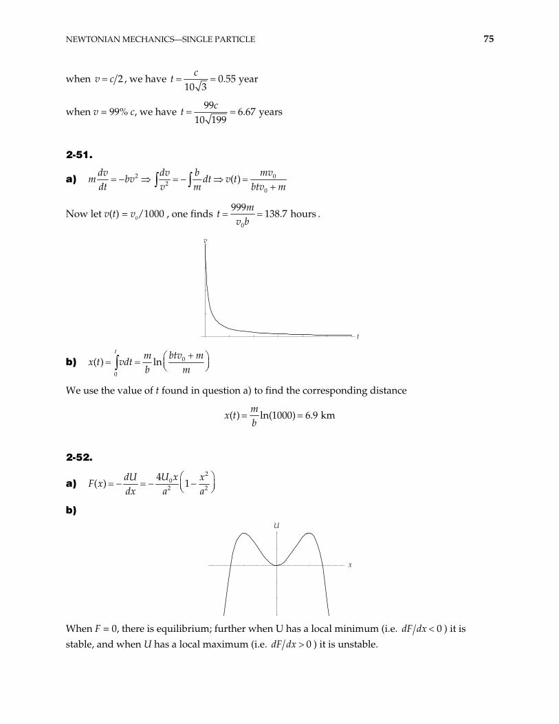
a) 2 02
0
( )mvdv dv b
m bv dt v tdt v m btv m
Now let v(t) = v0/1000 , one finds 0
999138.7 hours
mt
v b.
t
v
b) 0
0
( ) lnt btv mm
x t vdtb m
We use the value of t found in question a) to find the corresponding distance
( ) ln(1000) 6.9 kmm
x tb
2-52.
a) 2
02 2
4( ) 1
U xdU xF x
dx a a
b)
x
U
When F = 0, there is equilibrium; further when U has a local minimum (i.e. 0dF dx ) it is stable, and when U has a local maximum (i.e. 0dF dx ) it is unstable.
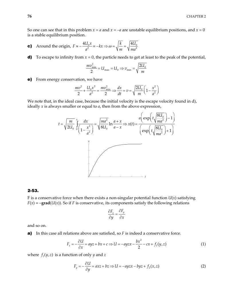
76 CHAPTER 2
So one can see that in this problem x = a and x = –a are unstable equilibrium positions, and x = 0 is a stable equilibrium position.
c) Around the origin, 0 02 2
4 4U x UkF kx
a m ma
d) To escape to infinity from x = 0, the particle needs to get at least to the peak of the potential,
2
0minmax 0 min
22
UmvU U v
m
e) From energy conservation, we have
2 22 2
0 0min2 2
21
2 2U x Umv dx x
va dt m
mv
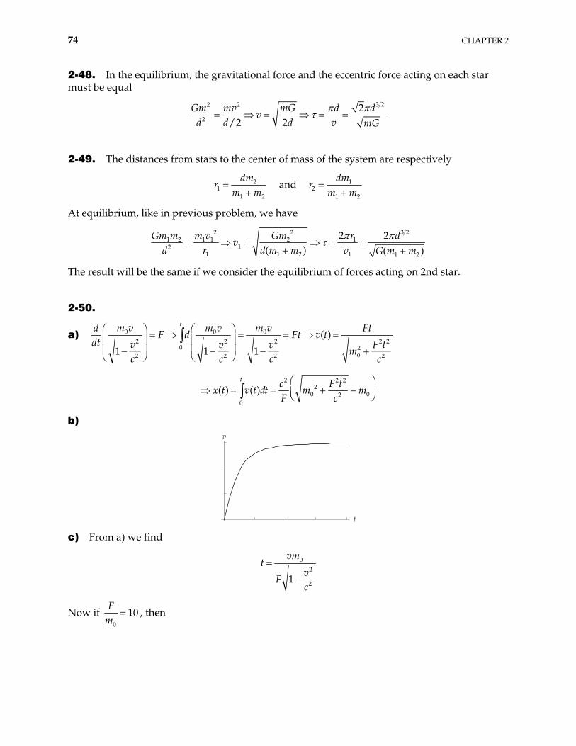
a
We note that, in the ideal case, because the initial velocity is the escape velocity found in d), ideally x is always smaller or equal to a, then from the above expression,
022
20 00 0
2 2
8exp 1
ln ( )2 8 81 exp 1
xU
a tmam dx ma a x
tU U a xx U
ta ma
t x
t
x
2-53.
F is a conservative force when there exists a non-singular potential function U(x) satisfying F(x) = –grad(U(x)). So if F is conservative, its components satisfy the following relations
yxFF
y x
and so on.
a) In this case all relations above are satisfied, so F is indeed a conservative force.
2
1( , )2x
U bxayz bx c U ayzx cx f y z
xF (1)
where is a function of only y and z 1( , )f y z
2( , )yU
axz bz U ayzx byz f x zy
F (2)
NEWTONIAN MECHANICS—SINGLE PARTICLE 77
where is a function of only x and z 2 ( , )f x z
3( , )U
axy by c U ayzx byz f y zzFz
(3)
then from (1), (2), (3) we find that
2
2
2bx
U axyz byz cx C
where C is a arbitrary constant.
b) Using the same method we find that F in this case is a conservative force, and its potential is
exp( ) lnU z x y z C
c) Using the same method we find that F in this case is a conservative force, and its potential is ( using the result of problem 1-31b):
lnU a r
2-54.
a) Terminal velocity means final steady velocity (here we assume that the potato reaches this velocity before the impact with the Earth) when the total force acting on the potato is zero.
mg = kmv and consequently 1000 m/skv g .
b)
0
0
0
( )x
v
F dx dv vdvg kv dt dx
dt m v g kv g kvdv
0max 2
0
ln 679.7 mg gv
xk k g kv
where v is the initial velocity of the potato. 0
2-55. Let’s denote and 0xv 0yv the initial horizontal and vertical velocity of the pumpkin. Evidently, 0x 0yv v in this problem.
0x xfx xx x f
x x
v vdv dvdxmkv dt x
dt v kv km F (1)
where the suffix f always denote the final value. From the second equality of (1), we have
0fktx
xf xx
dvdt v v e
kv (2)
Combining (1) and (2) we have
0 1 fktxf
vx
ke (3)
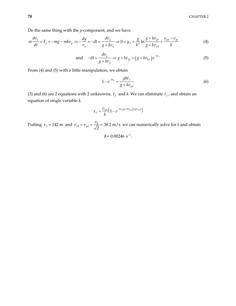
78 CHAPTER 2
Do the same thing with the y-component, and we have
02
0
0 lny y yf y yfy y f
y y y
dv dv g kv v vdy gm F mg mkv dt y
dt v g kv k g kv k (4)
and 0fkty
yf fy
dvdt g kv g kv e
g kv (5)
From (4) and (5) with a little manipulation, we obtain
0
1 fkt f
y
gkte
g kv (6)
(3) and (6) are 2 equations with 2 unknowns, ft and k. We can eliminate ft , and obtain an equation of single variable k.
0 00 1 f y xkt g kv gvxf
vx e
k
Putting and 142 mfx 00 0 38.2 m/s
2x yv
v v we can numerically solve for k and obtain
K= 0.00246 1s .
CHAPTER 3 Oscillations
3-1.
a) 4 2
10 2
gram cm10 dyne/cm1 1 10 10sec cm sec
2 2 10 gram 2 gram 2km
or,
0 1.6 Hz (1)
00
1 2sec
10
or,
0 0.63 sec (2)
b) 2 4 21 110 3 dyne-cm
2 2E kA
so that
44.5 10 ergE (3)
c) The maximum velocity is attained when the total energy of the oscillator is equal to the kinetic energy. Therefore,
2 4max
4
max
14.5 10 erg
2
2 4.5 10v
100
mv
79
80 CHAPTER 3
or,
max 30 cm/secv (4)
3-2.
a) The statement that at a certain time 1t t the maximum amplitude has decreased to one-half the initial value means that
10
12
tenx A e A0 (1)
or,
112
te (2)
so that
1 1
ln 2 0.69t t
(3)
Since , 1 10 sect
26.9 10 sec 1 (4)
b) According to Eq. (3.38), the angular frequency is
21 0
2 (5)
where, from Problem 3-1, 10 10 sec . Therefore,
22 21
2 6 1
10 6.9 10
110 1 6.9 10 sec
2
(6)
so that
51
10(1 2 40 10 ) sec
21 (7)
which can be written as
1 0 1 (8)
where
52.40 10 (9)
That is, 1 is only slightly different from 0 .
OSCILLATIONS 81
c) The decrement of the motion is defined to be e 1 where 1 1 1 . Then,
1 1.0445e
3-3. The initial kinetic energy (equal to the total energy) of the oscillator is 20
12
mv , where
m = 100 g and v . 0 1 cm/sec
a) Maximum displacement is achieved when the total energy is equal to the potential energy. Therefore,
2 20 0
1 12 2
mv kx
2
0 0 4
10 11 c
10 10m
x vk
m
or,
01
cm10
x (1)
b) The maximum potential energy is
2 4max 0
1 110 10
2 2U kx 2
or,
max 50 ergsU (2)
3-4.
a) Time average:
The position and velocity for a simple harmonic oscillator are given by
0sinx A t (1)
0 cosx A 0t (2)
where 0 k m
The time average of the kinetic energy is
21 12
t
t
T mx dt (3)
where 0
2 is the period of oscillation.
82 CHAPTER 3
By inserting (2) into (3), we obtain
2 2 20
1cos
2
t
t
T mA t0 dt (4)
or,
2 2
0
4mA
T (5)
In the same way, the time average of the potential energy is
2
2 20
2
1 12
1sin
2
4
t
t
t
t
U kx dt
kA t dt
kA (6)
and since 20 k m , (6) reduces to
2 2
0
4mA
U (7)
From (5) and (7) we see that
T U (8)
The result stated in (8) is reasonable to expect from the conservation of the total energy.
E T U (9)
This equality is valid instantaneously, as well as in the average. On the other hand, when T and U are expressed by (1) and (2), we notice that they are described by exactly the same function, displaced by a time 2 :
2 220
0
220
0
cos2
sin2
mAT t
mA tU t
(10)
Therefore, the time averages of T and U must be equal. Then, by taking time average of (9), we find
2E
T U (11)
b) Space average:
The space averages of the kinetic and potential energies are
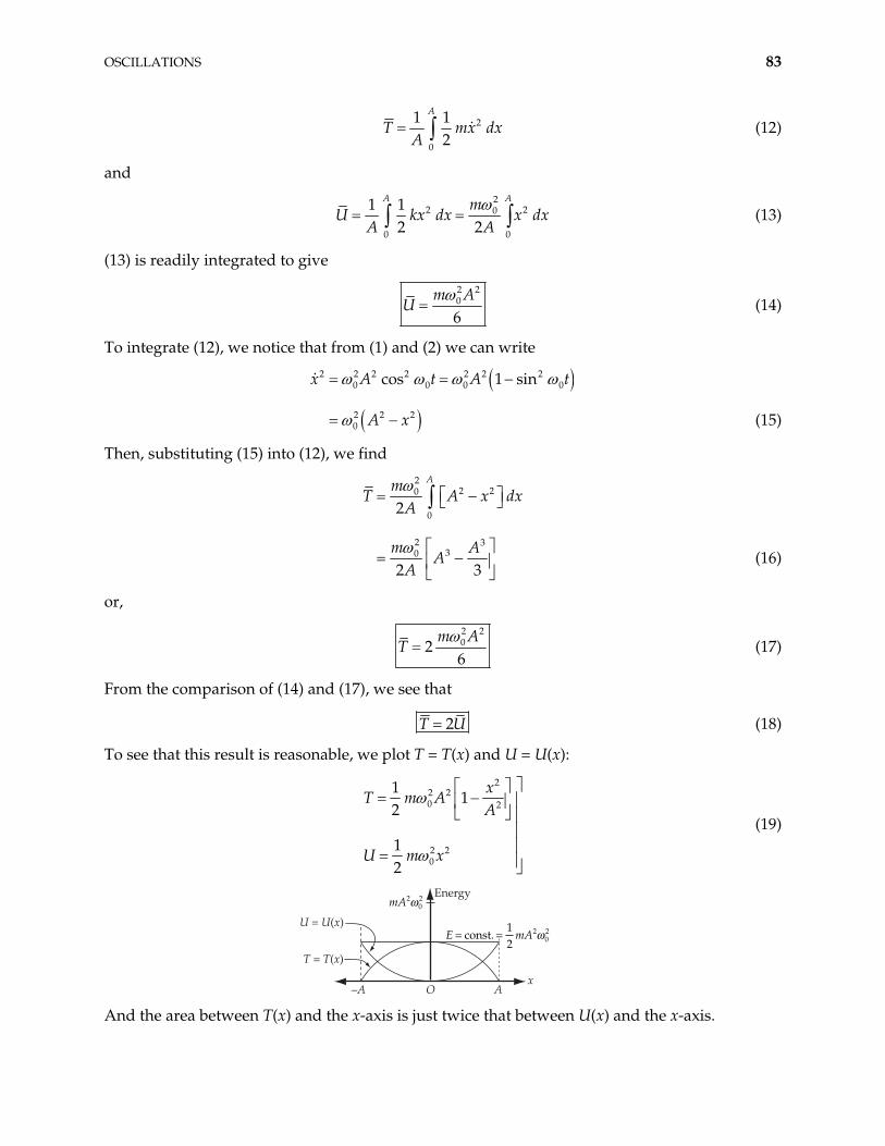
OSCILLATIONS 83
2
0
1 12
A
T mxA
dx (12)
and
2
2 0
0 0
1 12 2
A AmU kx dx x
A A2 dx (13)
(13) is readily integrated to give
2 20
6m A
U (14)
To integrate (12), we notice that from (1) and (2) we can write
2 2 2 2 2 2 20 0 0
2 2 20
cos 1 sinx A t A
A x
0t
(15)
Then, substituting (15) into (12), we find
22 20
0
2 330
2
2 3
AmT A x
A
m AA
A
dx
(16)
or,
2 2026
m AT (17)
From the comparison of (14) and (17), we see that
2T U (18)
To see that this result is reasonable, we plot T = T(x) and U = U(x):
22 20 2
2 20
11
2
12
xT m A
A
U m x
(19)
U = U(x)
T = T(x)
A
Energy
–A Ox
mA202!
E mA= =const.12
202!
And the area between T(x) and the x-axis is just twice that between U(x) and the x-axis.
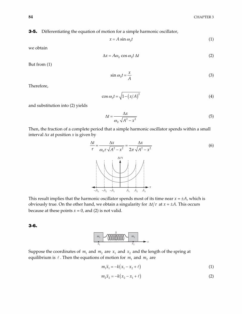
84 CHAPTER 3
3-5. Differentiating the equation of motion for a simple harmonic oscillator,
0sinx A t (1)
we obtain
0 0cosx A t t (2)
But from (1)
0sinx
tA
(3)
Therefore,
2
0cos 1t x A (4)
and substitution into (2) yields
2 2
0
xt
A x (5)
Then, the fraction of a complete period that a simple harmonic oscillator spends within a small interval x at position x is given by
2 2 2 2
0 2
t x x
A x A x (6)
–A1–A2–A3 A3A2A1
"t ⁄#
x
This result implies that the harmonic oscillator spends most of its time near x = A, which is obviously true. On the other hand, we obtain a singularity for t at x = A. This occurs because at these points x = 0, and (2) is not valid.
3-6.
x1 x2
k
x
m1 m2
Suppose the coordinates of m and are and x and the length of the spring at equilibrium is . Then the equations of motion for m and are
1 2m 1x 2
1 2m
1 1 1 2m x k x x (1)
2 2 2 1m x k x x (2)
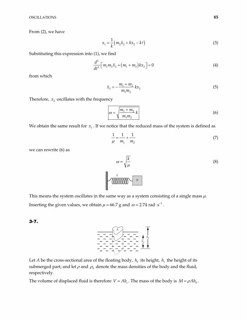
OSCILLATIONS 85
From (2), we have
1 2 2 21
x m x kx kk
(3)
Substituting this expression into (1), we find
2
1 2 2 1 2 22 0d
m m x m m kxdt
(4)
from which
1 22
1 2
m mx
m m 2kx (5)
Therefore, oscillates with the frequency 2x
1 2
1 2
m mk
m m (6)
We obtain the same result for . If we notice that the reduced mass of the system is defined as 1x
1 2
1 1 1m m
(7)
we can rewrite (6) as
k
(8)
kµ
This means the system oscillates in the same way as a system consisting of a single mass .
Inserting the given values, we obtain 66.7 g and 12.74 rad s .
3-7.
A
hb
hs
Let A be the cross-sectional area of the floating body, its height, the height of its submerged part; and let and
bh sh
0 denote the mass densities of the body and the fluid, respectively.
The volume of displaced fluid is therefore V sAh . The mass of the body is bM Ah .
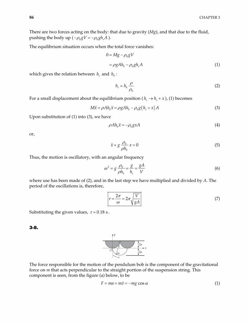
86 CHAPTER 3
There are two forces acting on the body: that due to gravity (Mg), and that due to the fluid, pushing the body up ( 0 0 sgV gh A ).
The equilibrium situation occurs when the total force vanishes:
0
0
0
b
Mg gV
gAh gh As (1)
which gives the relation between and : sh bh
0
s bh h (2)
For a small displacement about the equilibrium position ( ), (1) becomes s sh h x
0b b sMx Ah x gAh g h x A (3)
Upon substitution of (1) into (3), we have
0bAh x gxA (4)
or,
0 0b
x g xh
(5)
Thus, the motion is oscillatory, with an angular frequency
2 0
b s
g gAg
h h V (6)
where use has been made of (2), and in the last step we have multiplied and divided by A. The period of the oscillations is, therefore,
2
2VgA
(7)
Substituting the given values, 0 18 s .
3-8.
y
Oms
2a
2ax!
The force responsible for the motion of the pendulum bob is the component of the gravitational force on m that acts perpendicular to the straight portion of the suspension string. This component is seen, from the figure (a) below, to be
cosF ma mv mg (1)
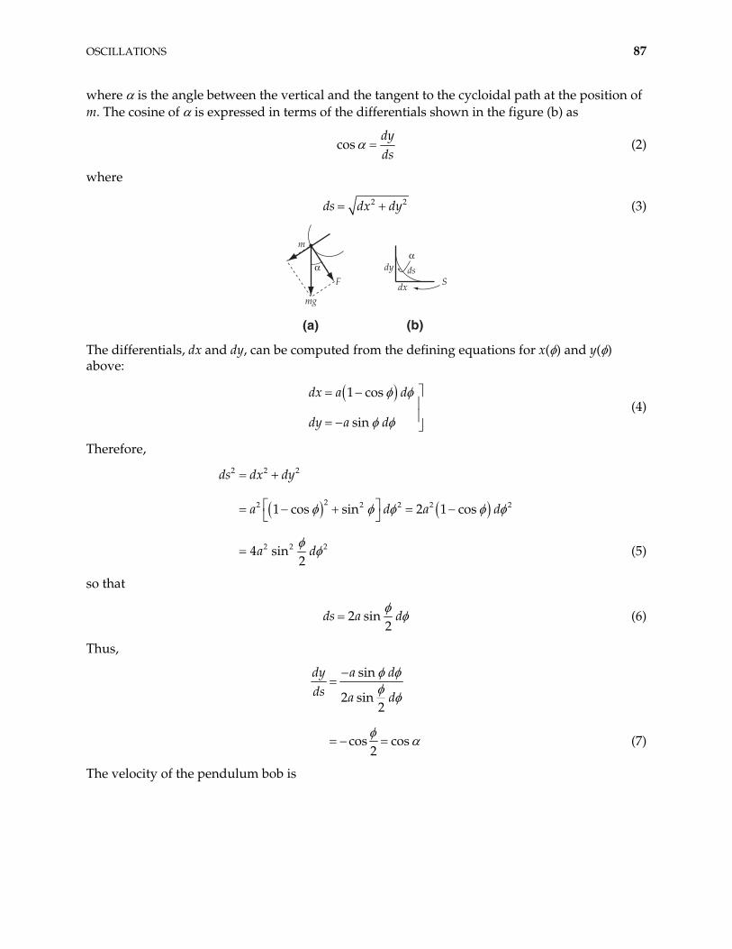
OSCILLATIONS 87
where is the angle between the vertical and the tangent to the cycloidal path at the position of m. The cosine of is expressed in terms of the differentials shown in the figure (b) as
cosdyds
(2)
where
2ds dx dy2 (3)
$$
m
mg
F dx
dyS
ds
(a) (b) The differentials, dx and dy, can be computed from the defining equations for x( ) and y( ) above:
1 cos
sin
dx a d
dy a d (4)
Therefore,
2 2 2
22 2 2 2
2 2 2
1 cos sin 2 1 cos
in2
ds dx dy
a d a
a d
2d
4 s (5)
so that
2 sin2
ds a d (6)
Thus,
sin
2 sin2
cos cos2
dy a dds a d
(7)
The velocity of the pendulum bob is
88 CHAPTER 3
2 sin2
4 cos2
ds dv a
dt dt
da
dt (8)
from which
2
24 cos2
dv a
dt (9)
Letting cos2
z be the new variable, and substituting (7) and (9) into (1), we have
4maz mgz (10)
or,
04g
z za
(11)
which is the standard equation for simple harmonic motion,
20 0z z (12)
If we identify
0g
(13)
where we have used the fact that . 4a
Thus, the motion is exactly isochronous, independent of the amplitude of the oscillations. This fact was discovered by Christian Huygene (1673).
3-9. The equation of motion for 00 t t is
0mx k x x F kx F kx0 (1)
while for , the equation is 0t t
0mx k x x kx kx0 (2)
It is convenient to define
0x x
which transforms (1) and (2) into
m k F ; 00 t t (3)
m k ; (4) 0t t
OSCILLATIONS 89
The homogeneous solutions for both (3) and (4) are of familiar form i t i tt Ae Be , where
k m . A particular solution for (3) is F k . Then the general solutions for (3) and (4) are
i t i tFAe Be
k; 00 t t (5)
i t i tCe De ; t (6) 0t
To determine the constants, we use the initial conditions: 00x t x and x(t = 0) = 0. Thus,
0 0t t 0 (7)
The conditions give two equations for A and B:
0
0
FA B
k
i A B
(8)
Then
2F
A Bk
and, from (5), we have
0 1 cosF
x x tk
; 00 t t (9)
Since for any physical motion, x and must be continuous, the values of x 0t t and
0t t are the initial conditions for t which are needed to determine C and D:
0 0
0 0
0 0
0 0
1 cos
sin
i t i t
i t i t
Ft t t Ce De
k
Ft t t i Ce De
k
(10)
The equations in (10) can be rewritten as:
0 0
0 0
0
0
1 cos
sin
i t i t
i t i t
FCe De t
k
iFCe De t
k
(11)
Then, by adding and subtracting one from the other, we obtain
0 0
0 0
12
12
i t i t
i t i t
FC e e
k
FD e e
k
(12)
90 CHAPTER 3
Substitution of (12) into (6) yields
0 0
0 0
0
1 12
2
cos cos
i t i t i t i t
i t t i t ti t i t
Fe e e e
k
Fe e e e
k
Ft t t
k (13)
Thus,
0 0cos cos ; F
t t t t tk 0x x (14)
3-10. The amplitude of a damped oscillator is expressed by
1costx t Ae t (1)
Since the amplitude decreases to 1 after n periods, we have e
1
21nT n (2)
Substituting this relation into the equation connecting 1 and 0 (the frequency of undamped oscillations), 2 2
1 02 , we have
2
2 2 210 1 1 2 2
11
2 4n n (3)
Therefore,
1 2
12 2
0
11
4 n (4)
so that
12 2
2
11
8 n
3-11. The total energy of a damped oscillator is
21 12 2
E t mx t kx t 2 (1)
where
1costx t Ae t (2)
1 1 1cos sintAe t tx t (3)
OSCILLATIONS 91
2 21 0 , 0
km
Substituting (2) and (3) into (1), we have
22 2 2 2 2
1 1 1
1 1 1
cos sin
2 sin cos
tAE t e m k t m t
m t t
2 (4)
Rewriting (4), we find the expression for E(t):
2
2 2 2 2 21 0 1cos2 sin 2
2tmA
e t t 0E t (5)
Taking the derivative of (5), we find the expression for dEdt
:
22 2 3
0 1
2 2 2 20 1 0
2 4 cos2
4 sin 2 2
tdE mAe t
t2dt (6)
The above formulas for E and dE reproduce the curves shown in Figure 3-7 of the text. To find the average rate of energy loss for a lightly damped oscillator, let us take
dt
0 . This means that the oscillator has time to complete some number of periods before its amplitude decreases considerably, i.e. the term 2 te does not change much in the time it takes to complete one period. The cosine and sine terms will average to nearly zero compared to the constant term in dE dt , and we obtain in this limit
2 2 20
tdEm A e
dt (7)
3-12.
mg
mg sin !
!!
The equation of motion is
sinm mg (1)
sing
(2)
If is sufficiently small, we can approximate sin , and (2) becomes

92 CHAPTER 3
g
(3)
which has the oscillatory solution
0 cost 0t (4)
where 0 g and where 0 is the amplitude. If there is the retarding force 2m g , the equation of motion becomes
sin 2m mg m g (5)
or setting sin and rewriting, we have
20 02 0 (6)
Comparing this equation with the standard equation for damped motion [Eq. (3.35)],
202x x x 0 (7)
we identify 0 . This is just the case of critical damping, so the solution for (t) is [see Eq. (3.43)]
0tt A Bt e (8)
For the initial conditions 00 and (0) = 0, we find
00 01 tt t e
3-13. For the case of critical damping, 0 . Therefore, the equation of motion becomes
22x x x 0 (1)
If we assume a solution of the form
tx t y t e (2)
we have
22
t t
t t
x ye ye
x ye ye ye t (3)
Substituting (3) into (1), we find
ye (4) 2 22 2 2t t t t t tye ye ye ye ye2 0
0
or,
y (5)
Therefore,
y t A Bt (6)
OSCILLATIONS 93
and
tx t A Bt e (7)
which is just Eq. (3.43).
3-14. For the case of overdamped oscillations, x(t) and x t are expressed by
21 2
t tx t e A e A e 2t (1)
2 2 21 2 1 2 2 2
t t te A e A e A e A e 2ttx t (2)
where 22
20 . Hyperbolic functions are defined as
cosh2
y ye ey , sinh
2
y ye ey (3)
or,
cosh sinh
cosh sinh
y
y
e y
e y
y
y (4)
Using (4) to rewrite (1) and (2), we have
1 2 2 1 2 2cosh sinh cosh sinht t A A t A A tx t (5)
and
1 2 1 2 2
2 2 2 2 2
cosh sinh cosh sinh
cosh sinh
x t t t A A t t
A A t t (6)
3-15. We are asked to simply plot the following equations from Example 3.2:
1costAe tx t (1)
1 1 1( ) cos sintAe t tv t (2)
with the values A = 1 cm 10 1 rad s , 10 1 s , and = rad. The position goes through
x = 0 a total of 15 times before dropping to 0.01 of its initial amplitude. An exploded (or zoomed) view of figure (b), shown here as figure (B), is the best for determining this number, as is easily shown.
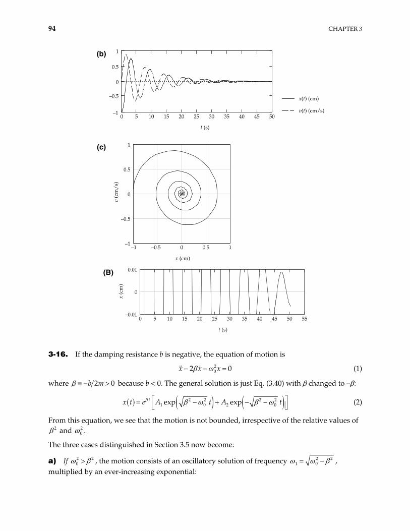
94 CHAPTER 3
–1 –0.5 0 0.5 1–1
–0.5
0
0.5
1
x (cm)
v (c
m/s
)0 5 10 15 20 25 30 35 40 45 50
–1
0
1
0.5
–0.5 x(t) (cm)
v(t) (cm/s)
t (s)
(b)
(c)
0 5 10 15 20 25 30 35 40 45 50 55
0
t (s)
x (c
m)
0.01
–0.01
(B)
3-16. If the damping resistance b is negative, the equation of motion is
202x x x 0 (1)
where 2b m 0 because b < 0. The general solution is just Eq. (3.40) with changed to – :
2 2 2 21 0 2exp expte A t A t0x t (2)
From this equation, we see that the motion is not bounded, irrespective of the relative values of 2 and 2
0 .
The three cases distinguished in Section 3.5 now become:
a) If 20
2 , the motion consists of an oscillatory solution of frequency 2 21 0 ,
multiplied by an ever-increasing exponential:
OSCILLATIONS 95
11 2
t i t i tx t e A e A e 1 (3)
b) If 20
2 , the solution is
tx t A Bt e (4)
which again is ever-increasing.
c) If 20
2 , the solution is:
21 2
t tx t e A e A e 2t (5)
where
2 22 0 (6)
This solution also increases continuously with time.
The tree cases describe motions in which the particle is either always moving away from its initial position, as in cases b) or c), or it is oscillating around its initial position, but with an amplitude that grows with the time, as in a).
Because b < 0, the medium in which the particle moves continually gives energy to the particle and the motion grows without bound.
3-17. For a damped, driven oscillator, the equation of motion is
202 cx x x A os t (1)
and the average kinetic energy is expressed as
2 2
22 2 20
4 4
mAT
2 (2)
Let the frequency n octaves above 0 be labeled 1 and let the frequency n octaves below 0 be labeled 2 ; that is
1 0
2 0
2
2
n
n (3)
The average kinetic energy for each case is
1
2 220
22 2 2 2 20 0 0
24 2 (4)2
n
n n
mA2
T (4)
2
2 220
22 2 2 2 20 0 0
24 2 (4)2
n
n n
mA2
T (5)
Multiplying the numerator and denominator of (5) by , we have 42 n
96 CHAPTER 3
2
2 220
22 2 2 2 20 0 0
24 2 (4)2
n
n n
mA2
T
Hence, we find
1
T T2
(6)
and the proposition is proven.
3-18. Since we are near resonance and there is only light damping, we have 0 R , where is the driving frequency. This gives 0 2Q . To obtain the total energy, we use the solution to the driven oscillator, neglecting the transients:
cosx t D t (1)
We then have
2
2 2 2 2 2 2 20
1 1 1sin ( ) cos
2 2 2 2mD
E mx kx t t m D20 (2)
The energy lost over one period is
2
02 2
Tm x xdt m D (3)
where 2T . Since 0 , we have
0
energy lost over one period 4 2E Q
(4)
which proves the assertion.
3-19. The amplitude of a damped oscillator is [Eq. (3.59)]
22 2 2
0 4
AD
2 (1)
At the resonance frequency, 20R
2 , D becomes
2 202
RA
D (2)
Let us find the frequency, = , at which the amplitude is 12 RD :
2 2 22 2 20 0
1 12 2 2 4
RA A
D (3)
Solving this equation for , we find
OSCILLATIONS 97
1 22
2 2 20 0 2
0
2 2 1 (4)
For a lightly damped oscillator, is small and the terms in 2 can be neglected. Therefore,
2 20 2 0 (5)
or,
00
1 (6)
which gives
0 0 2 (7)
We also can approximate R for a lightly damped oscillator:
2 20 2R 0 (8)
Therefore, Q for a lightly damped oscillator becomes
0 0
2Q (9)
3-20. From Eq. (3.66),
22 2 2 2
0
sin4
Ax t (1)
Therfore, the absolute value of the velocity amplitude v is given by
0 22 2 20 4
Av
2 (2)
The value of for v a maximum, which is labeled 0 v , is obtained from
0 0v
v (3)
and the value is 0v .
Since the Q of the oscillator is equal to 6, we can use Eqs. (3.63) and (3.64) to express in terms of 0 :
2
2 0
146 (4)
We need to find two frequencies, 1 and 2 , for which 0 max 2v v , where max 0 0v v . We find
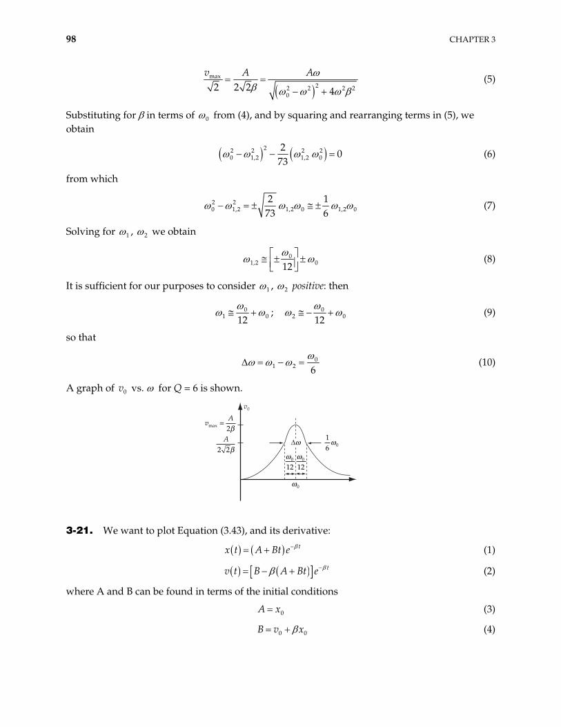
98 CHAPTER 3
max22 2 2
02 2 2 4
v A A2
(5)
Substituting for in terms of 0 from (4), and by squaring and rearranging terms in (5), we obtain
22 2 2 2
0 1,2 1,2 02
073
(6)
from which
2 20 1,2 1,2 0 1,2 0
2 173 6
(7)
Solving for 1 , 2 we obtain
01,2 012
(8)
It is sufficient for our purposes to consider 1 , 2 positive: then
01 012
; 02 12 0 (9)
so that
01 2 6
(10)
A graph of vs. for Q = 6 is shown. 0v
vA
max =2%
A2 2%
!0
12
16 0!
!0
12
!0
v0
"!
3-21. We want to plot Equation (3.43), and its derivative:
tx t A Bt e (1)
tv t B A Bt e (2)
where A and B can be found in terms of the initial conditions
0A x (3)
0B v x0 (4)
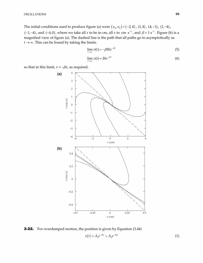
OSCILLATIONS 99
The initial conditions used to produce figure (a) were 0 0 2 4x v , (1 4) , , ( ,
, and , where we take all x to be in cm, all v in cm
(4 1) 1 4)
( 1 4) ( 4 0) 1s , and . Figure (b) is a magnified view of figure (a). The dashed line is the path that all paths go to asymptotically as t . This can be found by taking the limits.
11 s
lim ( ) t
tv t Bte (5)
lim ( ) t
tx t Bte (6)
so that in this limit, v = – x, as required.
–4 –2 0 2 4–4
–3
–2
–1
0
1
2
3
4
x (cm)
v (c
m/s
)
–0.5 –0.25 0 0.25 0.5
–0.4
–0.2
0
0.2
0.4
x (cm)
v (c
m/s
)
(a)
(b)
3-22. For overdamped motion, the position is given by Equation (3.44)
11 2
tx t A e A e 2t (1)
100 CHAPTER 3
The time derivative of the above equation is, of course, the velocity:
11 1 2 2
tv t A e A e 2t
2
(2)
a) At t = 0:
0 1x A A (3)
0 1 1 2v A A 2 (4)
The initial conditions and v can now be used to solve for the integration constants 0x 0 1A and
2A .
b) When 1 0A , we have v x0 2 0 and 2v t x t quite easily. For 1 0A , however, we have 1te1 1A 1xv t as t since 1 2 .
3-23. Firstly, we note that all the = solutions are just the negative of the = 0 solutions. The 2 solutions don’t make it all the way up to the initial “amplitude,” A , due to the retarding force. Higher means more damping, as one might expect. When damping is high, less oscillation is observable. In particular, 2 0 9 would be much better for a kitchen door than a smaller , e.g. the door closing ( = 0), or the closed door being bumped by someone who then changes his/her mind and does not go through the door ( 2 ).
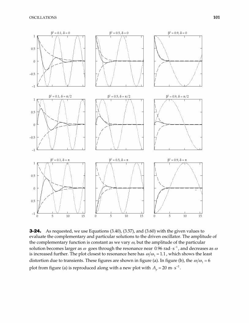
OSCILLATIONS 101
–1
–0.5
0
0.5
1%2 = 0.1, & = '/2
%2 = 0.9, & = 0
%2 = 0.9, & = '/2
0 5 10 15
%2 = 0.9, & = '
%2 = 0.5, & = 0
%2 = 0.5, & = '/2
0 5 10 15–1
0.5
0
0.5
1%2 = 0.1, & = '
0 5 10 15
%2 = 0.5, & = '
–0.5
0
0.5
1%2 = 0.1, & = 0
–1
3-24. As requested, we use Equations (3.40), (3.57), and (3.60) with the given values to evaluate the complementary and particular solutions to the driven oscillator. The amplitude of the complementary function is constant as we vary , but the amplitude of the particular solution becomes larger as goes through the resonance near 10 96 rad s , and decreases as is increased further. The plot closest to resonance here has 1 1 1 , which shows the least distortion due to transients. These figures are shown in figure (a). In figure (b), the 1 6
plot from figure (a) is reproduced along with a new plot with 220 m spA .
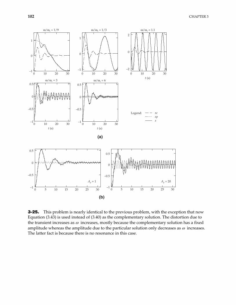
102 CHAPTER 3
–1
0
1
!/!1 = 1/3
0 10 20 30
–1
–0.5
0
0.5
0 10 20 30
!/!1 = 6
t (s)
–1
–0.5
0
0.5!/!1 = 3
0 10 20 30t (s)
–2
0
2
!/!1 = 1.1
0 10 20t (s)
30–1
0
1
!/!1 = 1/9
0 10 20 30
xcxpx
Legend:
(a)
0 5 10 15 20 25 30–1
–0.5
0
0.5
0 5 10 15 20 25 30–1
–0.5
0
0.5
(b)
Ap = 1 Ap = 20
3-25. This problem is nearly identical to the previous problem, with the exception that now Equation (3.43) is used instead of (3.40) as the complementary solution. The distortion due to the transient increases as increases, mostly because the complementary solution has a fixed amplitude whereas the amplitude due to the particular solution only decreases as increases. The latter fact is because there is no resonance in this case.
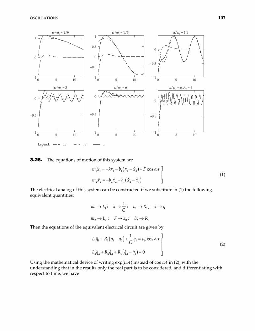
OSCILLATIONS 103
0 5 10–1
0
1
!/!1 = 1/9
0 5 10–1
–0.5
0
0.5
1!/!1 = 1/3
0 5 10–1
–0.5
0
!/!1 = 1.1
0 5 10–1
–0.5
0
!/!1 = 3
0 5 10–1
–0.5
0
!/!1 = 6
0 5 10–1
–0.5
0
!/!1 = 6, Ap = 6
xc xp xLegend:
3-26. The equations of motion of this system are
1 1 1 1 1 2
2 2 2 2 1 2 1
cosm x kx b x x F t
m x b x b x x (1)
The electrical analog of this system can be constructed if we substitute in (1) the following equivalent quantities:
m L ; 1 11
kC
; ; x q 1b R1
m L ; 2 2 0F ; 2 2b R
Then the equations of the equivalent electrical circuit are given by
1 1 1 1 2 1 0
2 2 2 2 1 2 1
1cos
0
L q R q q q tC
L q R q R q q
(2)
Using the mathematical device of writing exp(i t) instead of cos t in (2), with the understanding that in the results only the real part is to be considered, and differentiating with respect to time, we have
104 CHAPTER 3
11 1 1 1 2 0
2 2 2 2 1 2 1 0
i tIL I R I I i e
C
L I R I R I I
(3)
Then, the equivalent electrical circuit is as shown in the figure:
(0 cos !t
L1
L2R1
R2I1(t) I2(t)
1 2C
The impedance of the system Z is
11
Z i L i ZC 1 (4)
where is given by 1Z
1 1 2
1 1 1Z R R i L2
(5)
Then,
2 2
1 2 2 1 2 2 11 2 2 2
1 2 2
R R R R L i L RZ
R R L (6)
and substituting (6) into (4), we obtain
22 2 2 21 2 2 1 2 1 2 1 1 2 2
2 2 21 2 2
1R R R R L i R L L R R L
CZ
R R L (7)
3-27. From Eq. (3.89),
01
1cos sin
2 n nn
a a n t b n tF t (1)
We write
01
1cos
2 nn
F t a c n t n (2)
which can also be written using trigonometric relations as
01
1cos cos sin sin
2 n nn
t a c n t n t nF (3)
Comparing (3) with (2), we notice that if there exists a set of coefficients c such that n
OSCILLATIONS 105
cos
sin
n n n
n n n
c a
c b (4)
then (2) is equivalent to (1). In fact, from (4),
2 2 2
tan
n n n
nn
n
c a b
ba
(5)
with and b as given by Eqs. (3.91). na n
3-28. Since F(t) is an odd function, F(–t) = –F(t), according to Eq. (3.91) all the coefficients vanish identically, and the b are given by
na
n
0
0
0
0
sin
sin sin
1 1cos cos
2cos 0 cos
4 for odd
0 for even
nb F t n t dt
n t dt n t dt
n t n tn n
nn
nn
n
(1)
Thus,
2 1
2
42 1 0, 1, 2,
0
n
n
bn n
b
(2)
Then, we have
4 4 4
sin sin 3 sin 53 5
t t tF t (3)
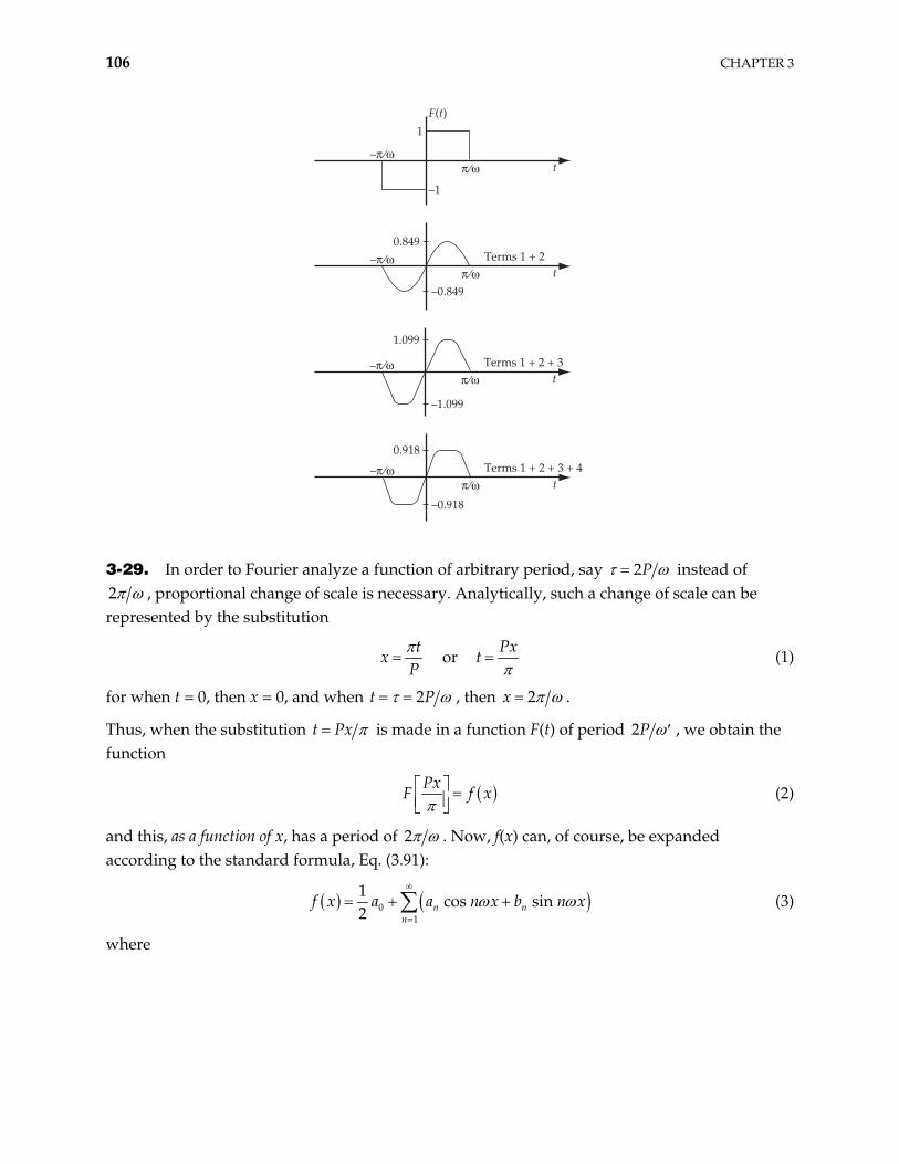
106 CHAPTER 3
F(t)
t
–1
1
–' ⁄!' ⁄!
Terms 1 + 2 t
–0.849
0.849–' ⁄!
' ⁄!
Terms 1 + 2 + 3 t
–1.099
1.099
–' ⁄!' ⁄!
Terms 1 + 2 + 3 + 4 t
–0.918
0.918
–' ⁄!' ⁄!
3-29. In order to Fourier analyze a function of arbitrary period, say 2P instead of 2 , proportional change of scale is necessary. Analytically, such a change of scale can be represented by the substitution
t
xP
or Px
t (1)
for when t = 0, then x = 0, and when 2Pt , then 2x .
Thus, when the substitution t Px is made in a function F(t) of period 2P , we obtain the function
Px
F f x (2)
and this, as a function of x, has a period of 2 . Now, f(x) can, of course, be expanded according to the standard formula, Eq. (3.91):
01
1cos sin
2 n nn
a a n x b n xf x (3)
where
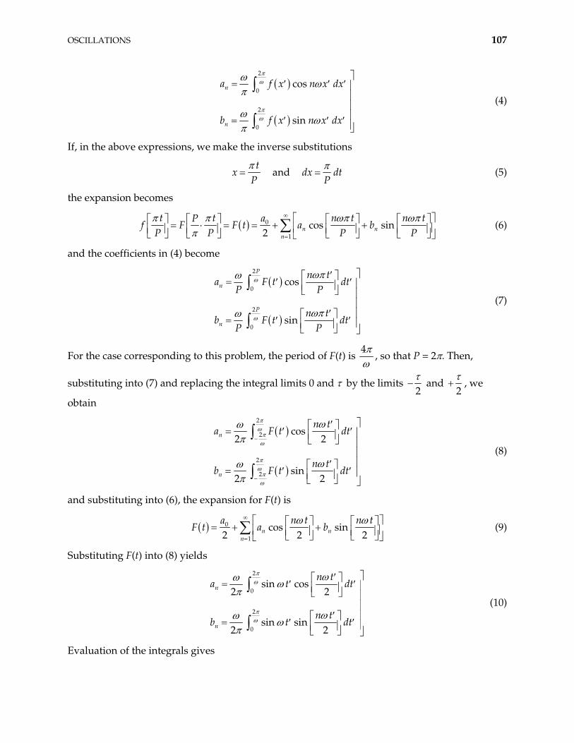
OSCILLATIONS 107
2
0
2
0
cos
sin
n
n
a f x n x d
b f x n x d
x
x
(4)
If, in the above expressions, we make the inverse substitutions
t
xP
and dx dtP
(5)
the expansion becomes
0
1
cos sin2 n n
n
t t n t n taPF t a b
P P P Pf F (6)
and the coefficients in (4) become
2
0
2
0
cos
sin
P
n
P
n
n ta F t
P P
n tb F t d
P P
dt
t
(7)
For the case corresponding to this problem, the period of F(t) is 4
, so that P = 2 . Then,
substituting into (7) and replacing the integral limits 0 and by the limits 2
and 2
, we
obtain
2
2
2
2
cos2 2
sin2 2
n
n
n ta F t
n tb F t
dt
dt
(8)
and substituting into (6), the expansion for F(t) is
0
1
cos sin2 2n n
n
n t n taa b
2F t (9)
Substituting F(t) into (8) yields
2
0
2
0
sin cos2 2
sin sin2 2
n
n
n ta t
n tb t
dt
dt
(10)
Evaluation of the integrals gives
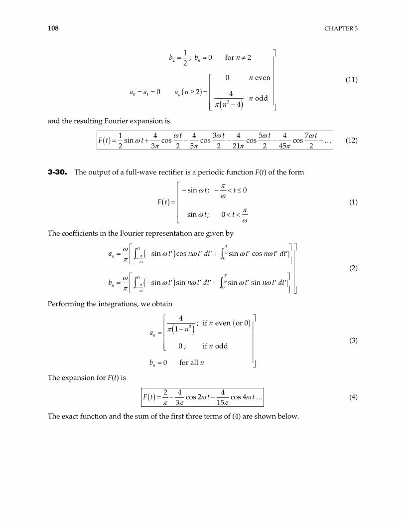
108 CHAPTER 3
2
0 1
2
1; 0 for 2
2
0 eve
0 2 4odd
4
n
n
b b n
n
a a a nn
n
n (11)
and the resulting Fourier expansion is
3 5 71 4 4 4 4
sin cos cos cos cos2 3 2 5 2 21 2 45 2
t t tF t t
t (12)
3-30. The output of a full-wave rectifier is a periodic function F(t) of the form
sin ; 0
sin ; 0
t t
F t
t t
(1)
The coefficients in the Fourier representation are given by
0
0
0
0
sin cos sin cos
sin sin sin sin
n
n
a t n t dt t n
b t n t dt t n
t dt
t dt
(2)
Performing the integrations, we obtain
2
4; if even or 0
1
0 ; if odd
0 for all
n
n
nna
n
b n
(3)
The expansion for F(t) is
2 4 4
cos 2 cos 43 15
t tF t (4)
The exact function and the sum of the first three terms of (4) are shown below.
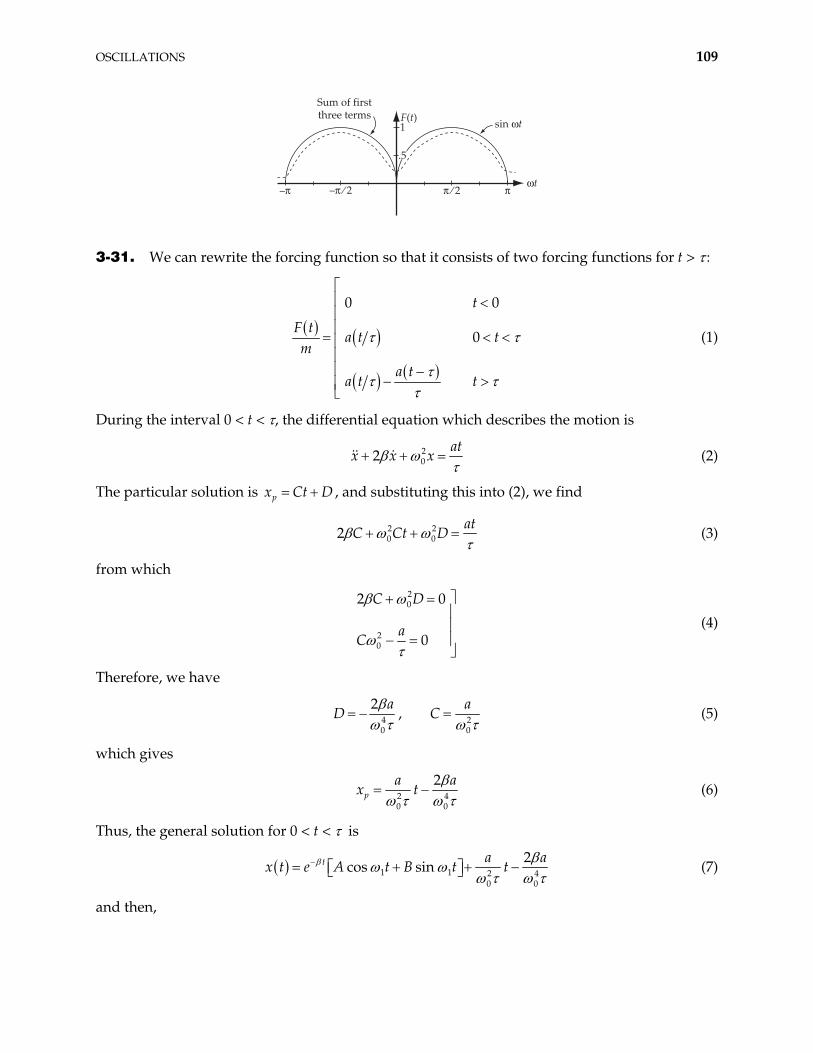
OSCILLATIONS 109
Sum of firstthree terms F(t) sin !t
!t–' ⁄ 2 ' ⁄ 2
1
–' '
.5
3-31. We can rewrite the forcing function so that it consists of two forcing functions for t > :
0 0
0
t
F ta t t
m
a ta t t
(1)
During the interval 0 < t < , the differential equation which describes the motion is
202
atx x x (2)
The particular solution is , and substituting this into (2), we find px Ct D
2 20 02
atC Ct D (3)
from which
20
20
2 0
0
C D
aC
(4)
Therefore, we have
40 0
2,
aD C 2
a (5)
which gives
20 0
2p
a ax t 4 (6)
Thus, the general solution for 0 < t < is
1 1 20 0
2cos sint a a
e A t B t t 4x t (7)
and then,
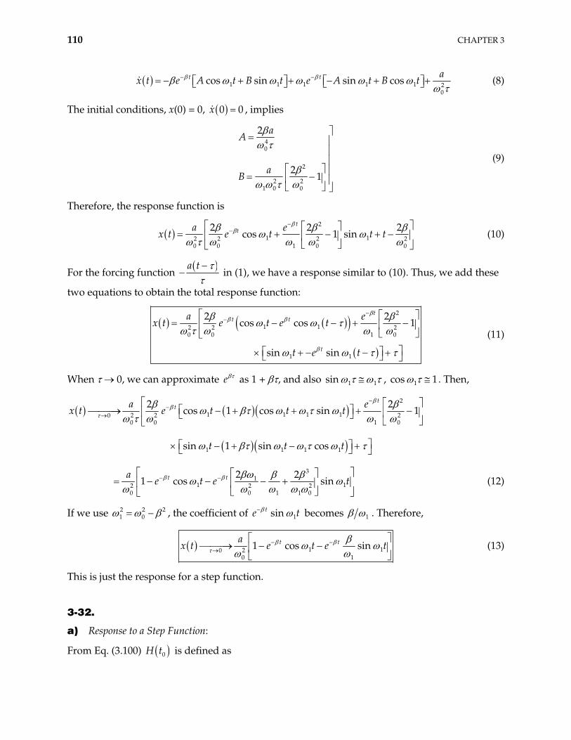
110 CHAPTER 3
1 1 1 1 1 20
cos sin sin cost t ax t e A t B t e A t B t (8)
The initial conditions, x(0) = 0, 0x 0 , implies
40
2
2 21 0 0
2
21
aA
aB
(9)
Therefore, the response function is
2
1 12 2 2 20 0 1 0 0
2 2cos 1 sin
tta e
e t t t2
x t (10)
For the forcing function a t
in (1), we have a response similar to (10). Thus, we add these
two equations to obtain the total response function:
2
1 12 2 20 0 1 0
1 1
2 2cos cos 1
sin sin
tt t
t
a ex t e t e t
t e t
(11)
When 0, we can approximate e as 1 + , and also 1 1sin , co 1s 1. Then,
2
1 1 1 12 2 200 0 1 0
1 1 1 1
31
1 12 2 20 0 1 1 0
2 2cos 1 cos sin 1
sin 1 sin cos
2 21 cos sin
tt
t t
a ex t e t t t
t t t
ae t e t
2
(12)
If we use 2 21 0 , the coefficient of 1sinte t becomes 1 . Therefore,
1200 1
1 cos sint tae t e t1x t (13)
This is just the response for a step function.
3-32.
a) Response to a Step Function:
From Eq. (3.100) 0H t is defined as
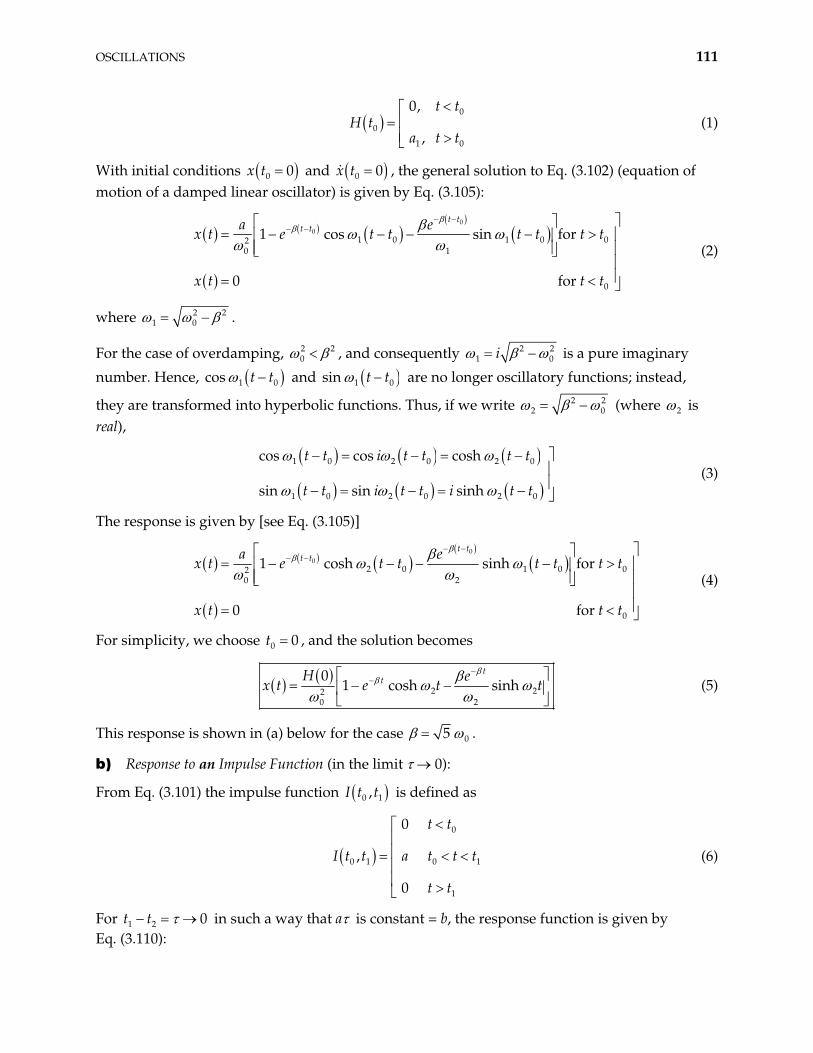
OSCILLATIONS 111
0
0
1 0
0,
,
t tH t
a t t (1)
With initial conditions 0 0x t and 0 0x t , the general solution to Eq. (3.102) (equation of motion of a damped linear oscillator) is given by Eq. (3.105):
00
1 0 1 0 020 1
0
1 cos sin for
0 f
t tt ta e
x t e t t t t t t
x t t tor
(2)
where 2 21 0 .
For the case of overdamping, 20
2 , and consequently 21 i 2
0 is a pure imaginary
number. Hence, 1cos t t0 and 1 0t tsin are no longer oscillatory functions; instead,
they are transformed into hyperbolic functions. Thus, if we write 22 0
2 (where 2 is real),
1 0 2 0 2 0
1 0 2 0 2 0
cos cos cosh
sin sin sinh
t t i t t t t
t t i t t i t t (3)
The response is given by [see Eq. (3.105)]
00
2 0 1 0 020 2
0
1 cosh sinh for
0 f
t tt ta e
x t e t t t t t t
x t t tor
(4)
For simplicity, we choose t , and the solution becomes 0 0
220 2
01 cosh sinh
ttH e
e t t2x t (5)
This response is shown in (a) below for the case 05 .
b) Response to an Impulse Function (in the limit 0):
From Eq. (3.101) the impulse function 0 1,I t t is defined as
0
0 1 0 1
1
0
,
0
t t
I t t a t t t
t t
(6)
For t t1 2 0 in such a way that a is constant = b, the response function is given by Eq. (3.110):
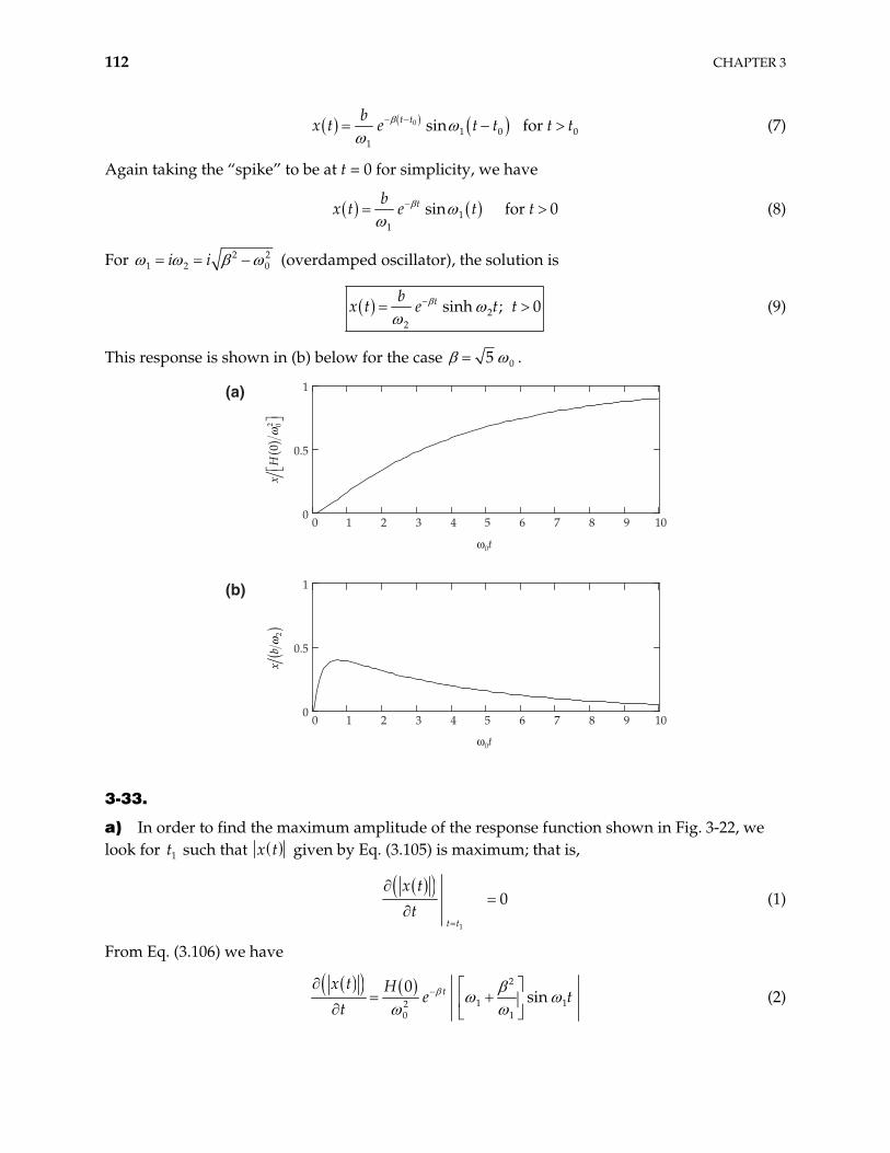
112 CHAPTER 3
01 0
1
sin for t tbe t t t t0x t (7)
Again taking the “spike” to be at t = 0 for simplicity, we have
11
sin for 0tbx t e t t (8)
For 21 2i i 2
0 (overdamped oscillator), the solution is
22
sinh ; 0tbx t e t t (9)
This response is shown in (b) below for the case 05 .
0 1 2 3 4 5 6 7 8 90
0.5
1
10
!0t
xH
002
()) *
+ ,!
0 1 2 3 4 5 6 7 8 90
0.5
1
10
!0t
()
xb
!2
(a)
(b)
3-33.
a) In order to find the maximum amplitude of the response function shown in Fig. 3-22, we look for such that 1t x t given by Eq. (3.105) is maximum; that is,
1
0t t
x t
t (1)
From Eq. (3.106) we have
2
120 1
0sintx t H
et 1t (2)
OSCILLATIONS 113
For 00.2 , 2 21 0 0.98 0 . Evidently, 1 1t makes (2) vanish. (This is the
absolute maximum, as can be seen from Fig. 3-22.)
Then, substituting into Eq. (3.105), the maximum amplitude is given by
11 2max
0
1a
x t x t e (3)
or,
1 20
1.53a
x t (4)
b) In the same way we find the maximum amplitude of the response function shown in Fig. 3-24 by using x(t) given in Eq. (3.110); then,
0
11
1 0 1 01
cos sint t
t tt t
x tbe t t t t
t (5)
If (5) is to vanish, is given by 1t
1 111 0
1 1
1 1tan tan 4.9
1
1.37t t (6)
Substituting (6) into Eq. (3.110), we obtain (for 00.2 )
11.37
1max0
sin 1.370.98
bx t ex t (7)
or,
10
0.76a
x t (8)
3-34. The response function of an undamped ( = 0) linear oscillator for an impulse function
I(0, ) , with 0
2, can be obtained from Eqs. (3.105) and (3.108) if we make the following
substitutions:
1 0
0 10
0 ;
20 ;t t
(1)
(For convenience we have assumed that the impulse forcing function is applied at t = 0.)
Hence, after substituting we have
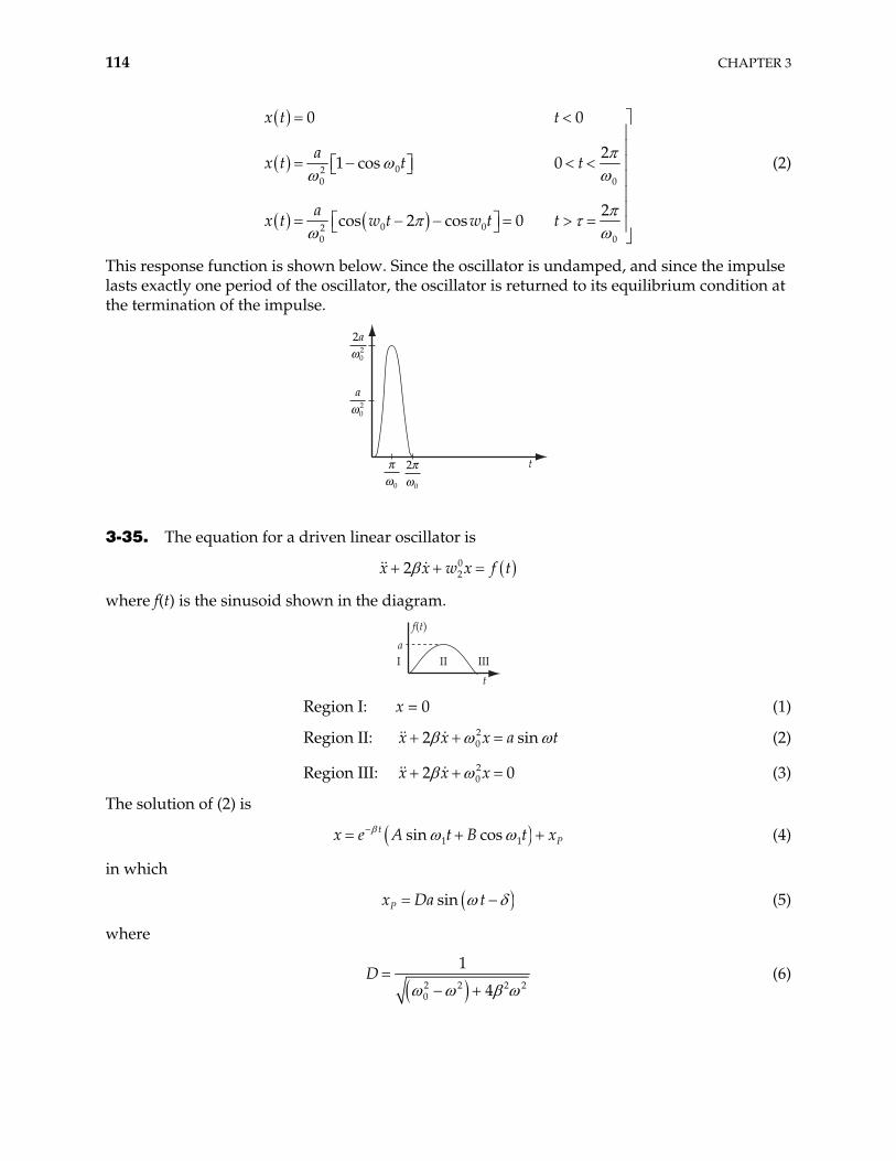
114 CHAPTER 3
020 0
0 020 0
0 0
21 cos 0
2cos 2 cos 0
x t t
at t
ax t w t w t t
x t (2)
This response function is shown below. Since the oscillator is undamped, and since the impulse lasts exactly one period of the oscillator, the oscillator is returned to its equilibrium condition at the termination of the impulse.
t
02
a!
2
0
'!0
'!
2
02a
!
3-35. The equation for a driven linear oscillator is
022x x w x f t
where f(t) is the sinusoid shown in the diagram.
f(t)
I II III
t
a
Region I: x = 0 (1)
Region II: x x 202 x a sin t
0
(2)
Region III: x x 202 x (3)
The solution of (2) is
1 1sin costPx e A t B t x (4)
in which
sinPx Da t (5)
where
2 2 20
1
4D
2 (6)
OSCILLATIONS 115
120
2tan 2 (7)
Thus,
1 1sin cos sint A t B t D a tx e (8)
The initial condition x(0) = 0 gives
sinB aD (9)
and 0 0x
1 cos 0B A Da
or,
1
sin cosaD
A (10)
The solution of (3) is
1sin costx t e A t B t1 (11)
We require that x t and x t for regions II and III match at t . The condition that
II IIIx x gives
sin cos sin sin cosB Da e A Be A
where 1 or,
sin
cot cotsin
aDA B eA B (12)
The condition that II IIIx x gives
1 1
1 1
sin cos cos cos sin
sin cos cos sin
e A B aD e A B
e A B e A B
or,
1 1
1 1
cos sin sin cos
sin cos sin cos cos
A B
A B e aD
or,
1 1
1 1 1
sin cos sin cos coscos sin cos sin cos sin
DaA B A B e (13)
116 CHAPTER 3
Substituting into (13) from (12), we have
1 1
1
1 1
1 1
cos sin cos sin cos sincos sin sin
cos sin cos sin cos sin sin coscos sin sin sin cos sin
B
aDe
(14)
from which
11
sin sin cos sin cos sina
D DeB a (15)
Using (12), we can find A :
sin
cot cotsin
aD eB BA A (16)
Substituting for A, B, and B from (10), (9), and (15), we have
1 1 1
cossin cos sin 1 cos
aDA aD e e (17)
Thus, we obtained all constants giving us the response functions explicitly.
3-36. With the initial conditions, 0x t x0 and 0x t x0 , the solution for a step function for given by Eq. (3.103) yields 0t t
0 01 0 22
0 1 1
;x xa a
A x A 20 1
(1)
Therefore, the response to 0H t for the initial conditions above can be expressed as
0
0 0
0 00 1 0 1 0
1 1
1 0 1 020 1
cos sin
1 cos sin for
t t
t t t t
x xx t e x t t t t
ae t t e t t 0t t
(2)
The response to an impulse function 0 1 1,I t t H t , for the above initial conditions will then be
given by (2) for t t and by a superposition of solutions for 0 t1 0H t and for 1H t
1t taken
individually for . We must be careful, however, because the solution for t must be equal that given by (2) for . This can be insured by using as a solution for
1t t
1t t 1H t Eq. (3.103) with initial conditions 0 0x , 0 0x , and using t instead of t in the expression. 1 0
The solution for t is then 1t
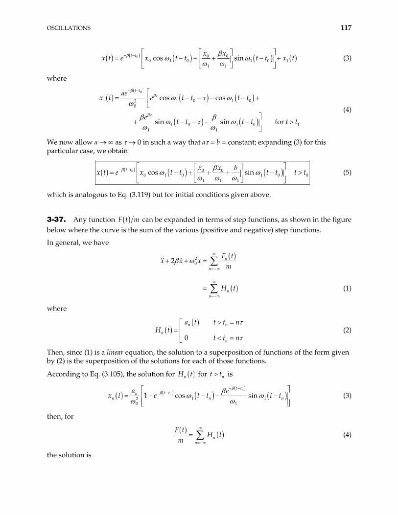
OSCILLATIONS 117
0 0 00 1 0 1 0 1
1 1
cos sint t x xt e x t t t t x tx (3)
where
0
11 1 0 1 02
0
1 0 1 01 1
cos cos
sin sin for
t taex t e t t t t
et t t t
e
t t1
(4)
We now allow a as 0 in such a way that a = b = constant; expanding (3) for this particular case, we obtain
0 0 00 1 0 1 0
1 1 1
cos sint t x x bx t e x t t t t t t0 (5)
which is analogous to Eq. (3.119) but for initial conditions given above.
3-37. Any function F t m can be expanded in terms of step functions, as shown in the figure below where the curve is the sum of the various (positive and negative) step functions.
In general, we have
202 n
n
nn
F tx x x
m
H t (1)
where
0
n n
n
n
a t t t nH t
t t n (2)
Then, since (1) is a linear equation, the solution to a superposition of functions of the form given by (2) is the superposition of the solutions for each of those functions.
According to Eq. (3.105), the solution for nH t for is nt t
120 1
1 cos sinn
n
t tt tn
n na e
e t t t t1 nx t (3)
then, for
nn
F tH t
m (4)
the solution is
118 CHAPTER 3
1 120 1
11 cos sin
nn
t tt t
n nn
n n n nn n
ex t H t e t t t t
mH t G t F t G t
n
(5)
where
1 12
0 1
11 cos sin ;
0
nn
t tt t
n n
n
n
ee t t t t
mG t
t t
nt t (6)
or, comparing with (3)
,
0
n n
n
n
x t ma t tG t
t t
n (7)
Therefore, the Green’s function is the response to the unit step.
Hn(t)
F tm( )
tn+1tn t
3-38. The solution for x(t) according to Green’s method is
010
1
,
sin sin
t
t t t t
x t F t G t t dt
Fe t e t t
mdt (1)
Using the trigonometric identity,
1 1 1 11
sin sin cos cos2
t t t t t t 1t (2)
we have
OSCILLATIONS 119
01 1 1 1
1 0 0
cos cos2
t ttt tF e
x t dt e t t dt e t tm
(3)
Making the change of variable, 1 1z t t , for the first integral and 1 1y t t for the second integral, we find
1 1
1 11
1 1
0
1 1 1
cos cos2
t tz yt tt
t t
F e e edz e z dy e y
m1x t (4)
After evaluating the integrals and rearranging terms, we obtain
02 22 2
1 1
2 2 21
2 2 2 11 1
sin2 cos
sin2 cos
t
t
Fx t
m
te t
te t
(5)
3-39.
sin 0
0 2
t tF t
t
From Equations 3.89, 3.90, and 3.91, we have
01
1cos sin
2 n nn
F t a a n t b n t
0
2cosna F t n t dt
0
2sinnb F t n t dt
0
sin cosna t n t dt
0 0
2sina t dt
1 0sin cos 0a t t dt
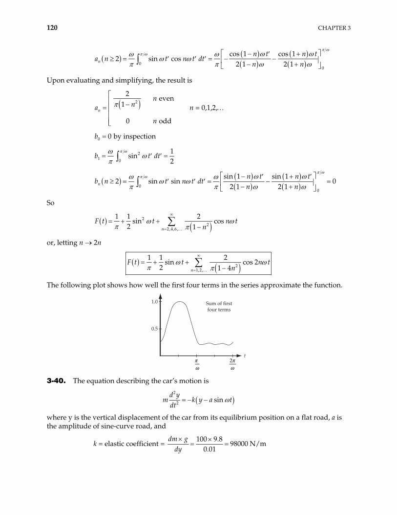
120 CHAPTER 3
0
0
cos 1 cos 12 sin cos
2 1 2 1nn t n t
a n t n t dtn n
Upon evaluating and simplifying, the result is
2
2 even
1
0 o
n
nna
n dd
n = 0,1,2,
0 0 by inspectionb
21 0
1sin
2b t dt
0
0
sin 1 sin 12 sin sin
2 1 2 1nn t n t
b n t n t dtn n
0
So
22
2,4,6,
1 1 2sin cos
2 1n
F t t n tn
or, letting n 2n
2
1,2,
1 1 2sin cos 2
2 1 4n
t n tn
F t
The following plot shows how well the first four terms in the series approximate the function.
Sum of firstfour terms
t'!
2'!
1.0
0.5
3-40. The equation describing the car’s motion is
2
2 sind y
m k y adt
t
where y is the vertical displacement of the car from its equilibrium position on a flat road, a is the amplitude of sine-curve road, and
k = elastic coefficient = 100 9.8
98000 N/m0.01
dm gdy
OSCILLATIONS 121
02174
v rad/s with and being the car’s speed and wavelength of sine-curve road.
The solution of the motion equation can be cast in the form
0v
2
00 2 2
0
cos sina
y t B t t with 0 9.9 rad/skm
We see that the oscillation with angular frequency has amplitude
20
2 20
0.16 mma
A
The minus sign just implies that the spring is compressed.
3-41.
a) The general solution of the given differential equation is (see Equation (3.37))
2 2 2 21 0 2exp exp expx t t A t A t 0
and
2 2 2 21 0 2
2 2 2 2 2 20 1 0 2 0
( ) exp exp exp
exp exp exp
v t x t t A t A t
t A t A t
0
at t = 0, , v t 0( )x t x 0( ) v
0 01 0 2 2
0
12
v xA x and 0 0
1 0 2 20
12
v xA x (1)
b)
i) Underdamped, 0
2
In this case, instead of using above parameterization, it is more convenient to work with the following parameterization
2 20( ) exp cosx t A t t (2)
2 2 2 2 2 20 0 0( ) exp cos sinv t A t t t (3)
Using initial conditions of x(t) and v(t), we find
2
20 002 2
00
x vx
2A and
0
02 20
tan ( )
vx
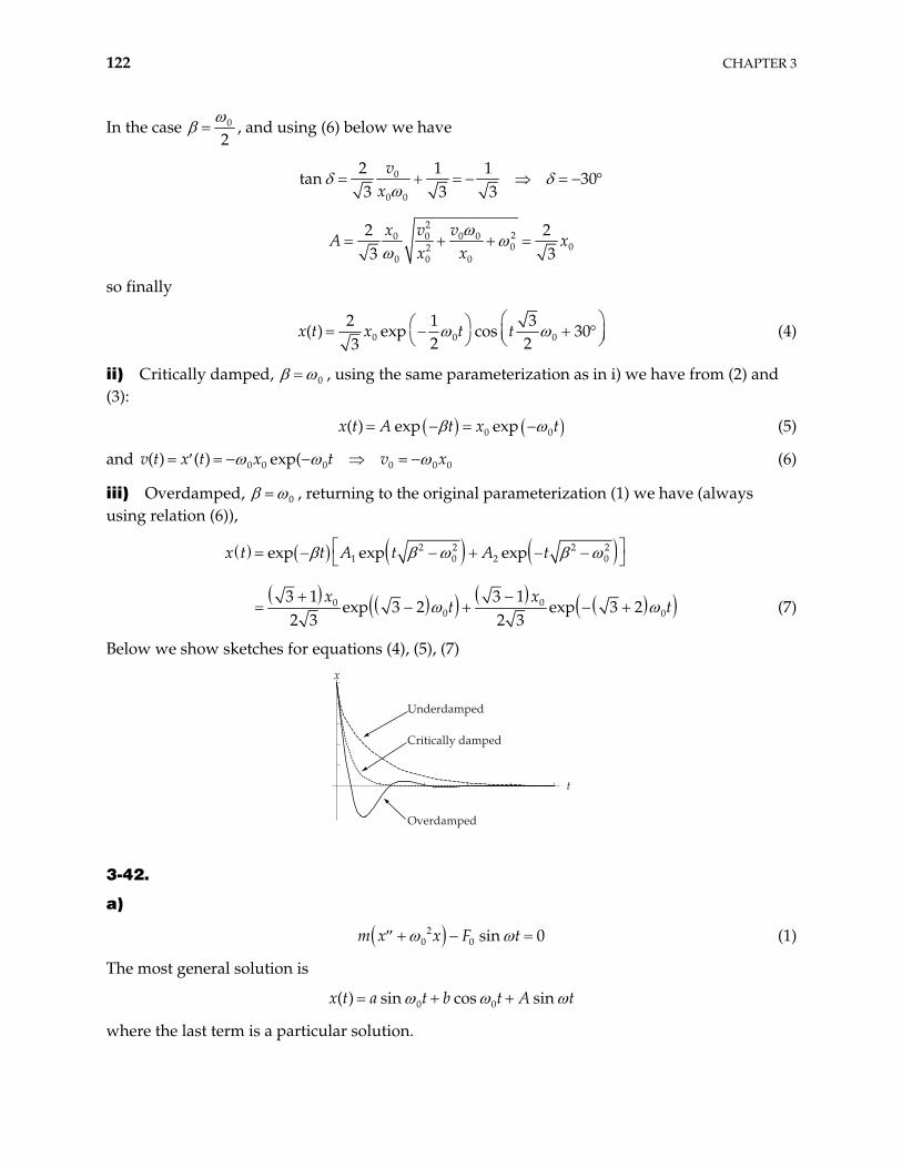
122 CHAPTER 3
In the case 0
2, and using (6) below we have
0
0 0
2 1 130
3 3 3v
xtan
2
20 0 0 00 02
0 0 0
2 23 3
x v vA x
x x
so finally
0 0 02 1 3
( ) exp cos 302 23
x t tx t (4)
ii) Critically damped, 0 , using the same parameterization as in i) we have from (2) and (3):
0( ) exp expx t A t x t0 (5)
and 0 0 0 0 0 0( ) ( ) exp(v t x t x t v x (6)
iii) Overdamped, 0 , returning to the original parameterization (1) we have (always using relation (6)),
2 2 2 21 0 2 0
0 00
exp exp exp
3 1 3 1exp 3 2 exp 3 2
2 3 2 3
x t t A t A t
x xt 0t (7)
Below we show sketches for equations (4), (5), (7)
t
x
Underdamped
Critically damped
Overdamped
3-42.
a)
20 0 sin 0m x x F t (1)
The most general solution is
0 0( ) sin cos sinx t a t b t A t
where the last term is a particular solution.
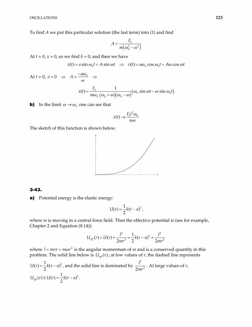
OSCILLATIONS 123
To find A we put this particular solution (the last term) into (1) and find
02 20
FA
m
At t = 0, x = 0, so we find b = 0, and then we have
x t 0 0 0( ) sin sin ( ) cos cosa t A t v t a t A t
At t = 0, 00a
v A
00 0
0 0 0
1( ) sin sin
Ft t
mx t
b) In the limit 0 one can see that
3
0 0( )6
F tx t
m
The sketch of this function is shown below.
t
x
3-43.
a) Potential energy is the elastic energy:
21( ) ( )
2U r k r a ,
where m is moving in a central force field. Then the effective potential is (see for example, Chapter 2 and Equation (8.14)):
2 2
22 2
1( ) ( ) ( )
2 2 2effl l
U r k r amr mr
U r
where l m 2vr m r is the angular momentum of m and is a conserved quantity in this problem. The solid line below is U ; at low values of r, the dashed line represents ( )eff r
21( )
2k r a( )U r , and the solid line is dominated by
2
22lmr
. At large values of r,
2( )k r a1
( ) ( )2effU r U r .
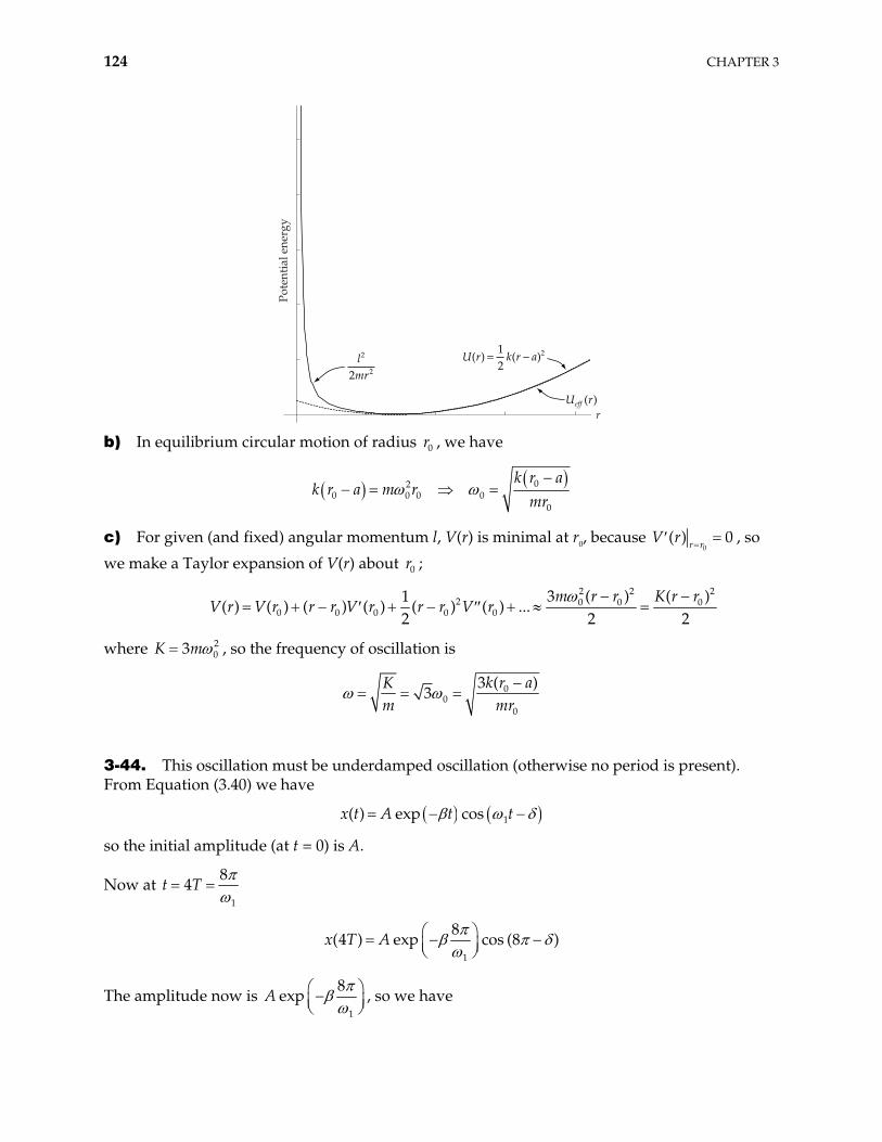
124 CHAPTER 3
Pote
ntia
l ene
rgy
r
U r k r a( ) ( )= -12
2lmr
2
22
U reff ( )
b) In equilibrium circular motion of radius , we have 0r
020 0 0 0
0
k r aa m r
mrk r
c) For given (and fixed) angular momentum l, V(r) is minimal at r0, because 0
( ) 0r rV r , so
we make a Taylor expansion of V(r) about ; 0r
2 2
2 0 0 00 0 0 0 0
3 ( ) ( )1( ) ( ) ( ) ( ) ( ) ( ) ...
2 2m r r K r r
V r V r r r V r r r V r2
2
where 203K m , so the frequency of oscillation is
00
0
3 ( )3
k r aKm mr
3-44. This oscillation must be underdamped oscillation (otherwise no period is present). From Equation (3.40) we have
1( ) exp cosx t A t t
so the initial amplitude (at t = 0) is A.
Now at 1
84t T
1
8(4 ) exp cos (8 )x T A
The amplitude now is 1
8expA , so we have
OSCILLATIONS 125
1
8exp1
A
A e
and because 20
21 , we finally find
12
0
8
64 1
3-45. Energy of a simple pendulum is 2
2mgl
where is the amplitude.
For a slightly damped oscillation ( ) exp( )t t .
Initial energy of pendulum is 2
2mgl
.
Energy of pendulum after one period, 2lg
T , is
2 2( ) exp ( 2 )2 2
mgl mglT T
So energy lost in one period is
2 21 exp 2 22 2
mgl mglT T mg 2l T
So energy lost after 7 days is
2 2(7 days)(7 days)mgl T mgl
T
This energy must be compensated by potential energy of the mass M as it falls h meters:
2 12(7 days) 0.01 s(7 days)Mh
h mglml
Mg
Knowing we can easily find the coefficient Q (see Equation (3.64))
22 2
022
1782 2 2
R
glQ

126 CHAPTER 3
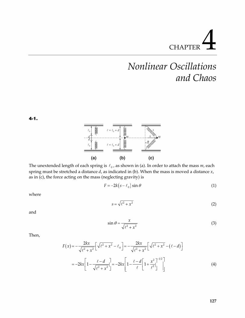
CHAPTER 4 Nonlinear Oscillations
and Chaos
4-1.
dd
!0
!0
(a) (b) (c)
! = !0 + d
! = !0 + d
m m
s
x
!
The unextended length of each spring is , as shown in (a). In order to attach the mass m, each spring must be stretched a distance d, as indicated in (b). When the mass is moved a distance x, as in (c), the force acting on the mass (neglecting gravity) is
0
02 siF k s n (1)
where
2s 2x (2)
and
2
sinx
x2 (3)
Then,
2 2 2 202 2 2 2
1 22
22 2
2 2
2 1 2 1 1
kx kxF x x x d
x x
d d xkx kx
x (4)
127
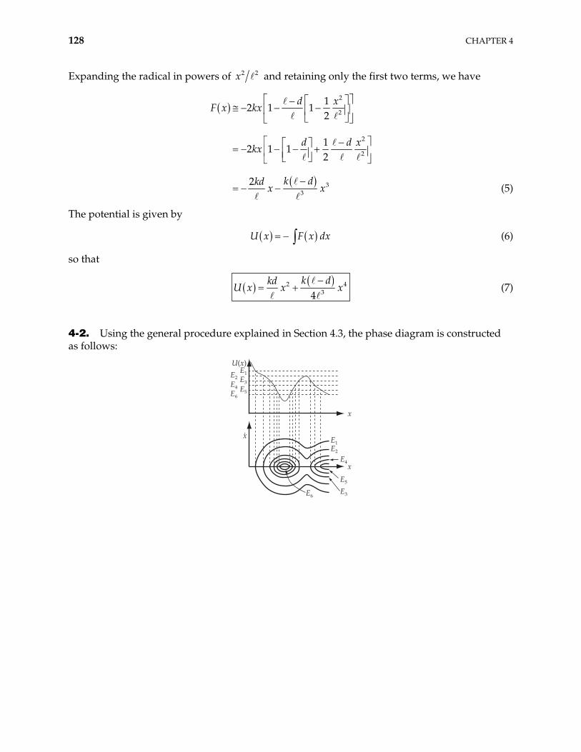
128 CHAPTER 4
Expanding the radical in powers of 2 2x and retaining only the first two terms, we have
2
2
2
2
33
12 1 1
2
12 1 1
2
2
d xF x kx
d dkx
k dkdx x
x
(5)
The potential is given by
(6) U x F x dx
so that
234
k dkdU x x x4 (7)
4-2. Using the general procedure explained in Section 4.3, the phase diagram is constructed as follows:
·x
x
x
E1
U(x)
E6E5
E4E3
E2
E6
E5
E4
E3
E2
E1
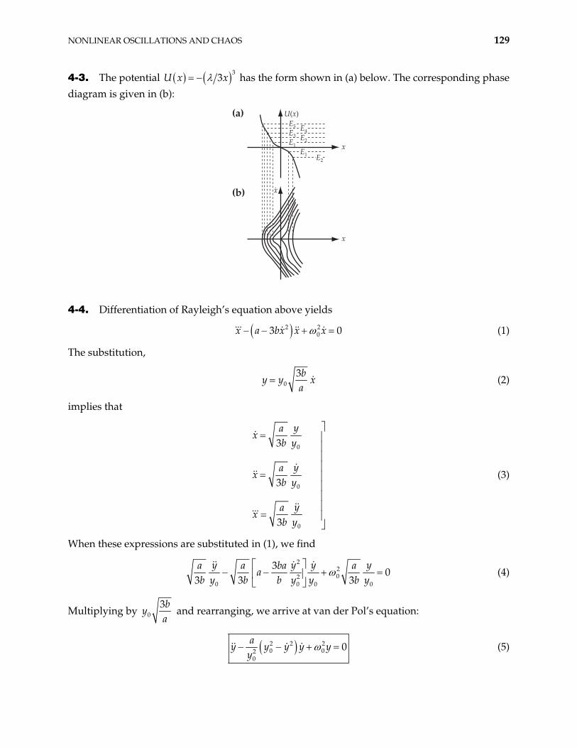
NONLINEAR OSCILLATIONS AND CHAOS 129
4-3. The potential 3
3xU x has the form shown in (a) below. The corresponding phase diagram is given in (b):
x
x
·x
U(x)E5 E4
E2
E1 E2
E3
E1
(a)
(b)
4-4. Differentiation of Rayleigh’s equation above yields
2 203x a bx x x 0 (1)
The substitution,
03b
y y xa
(2)
implies that
0
0
0
3
3
3
yax
b y
yax
b y
yax
b y
(3)
When these expressions are substituted in (1), we find
2
202
0 0 0
30
3 3 3y y ya a ba a
ab y b b y y b y0
y (4)
Multiplying by 03b
ya
and rearranging, we arrive at van der Pol’s equation:
2 2 20 02
0
0a
y y y y yy
(5)
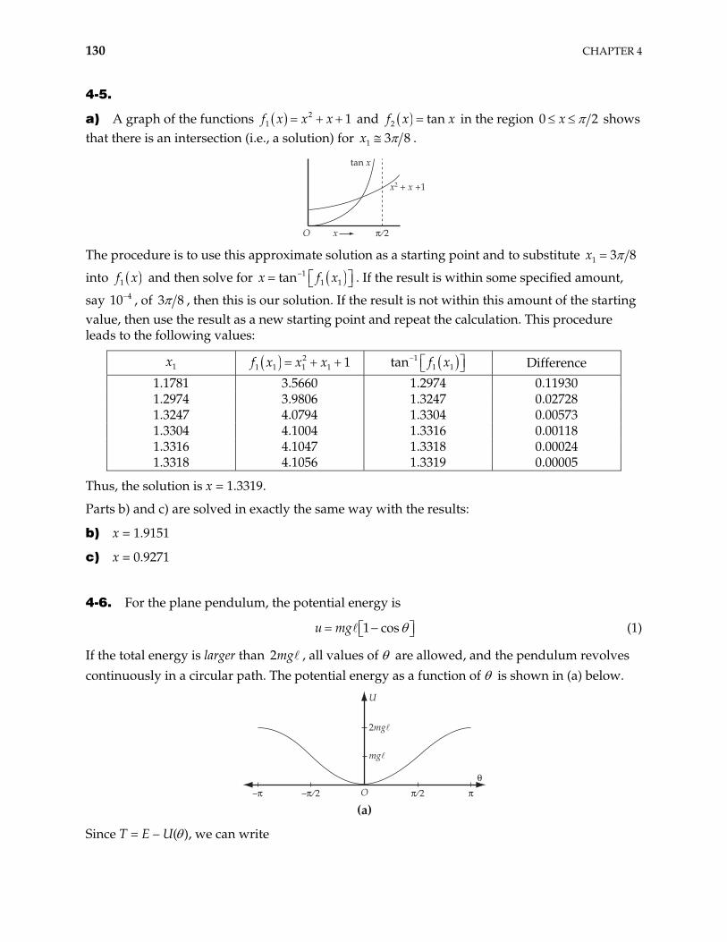
130 CHAPTER 4
4-5.
a) A graph of the functions 21 1f x x x and 2 tanf x x in the region 0 x 2 shows
that there is an intersection (i.e., a solution) for 1x 3 8 .
tan x
O x ! ⁄2
x2 + x +1
The procedure is to use this approximate solution as a starting point and to substitute 1 3 8x
into 1f x and then solve for 11 1tanx f x . If the result is within some specified amount,
say 10 , of 4 3 8 , then this is our solution. If the result is not within this amount of the starting value, then use the result as a new starting point and repeat the calculation. This procedure leads to the following values:
1x 21 1 1 1 1f x x x 1
1 1tan f x Difference 1.1781 3.5660 1.2974 0.11930 1.2974 3.9806 1.3247 0.02728 1.3247 4.0794 1.3304 0.00573 1.3304 4.1004 1.3316 0.00118 1.3316 4.1047 1.3318 0.00024 1.3318 4.1056 1.3319 0.00005
Thus, the solution is x = 1.3319.
Parts b) and c) are solved in exactly the same way with the results:
b) x = 1.9151
c) x = 0.9271
4-6. For the plane pendulum, the potential energy is
1 cosu mg (1)
If the total energy is larger than , all values of are allowed, and the pendulum revolves continuously in a circular path. The potential energy as a function of is shown in (a) below.
2mg
U
2mg!
mg!
–" –" ⁄2 " ⁄2O!
"
(a) Since T = E – U( ), we can write
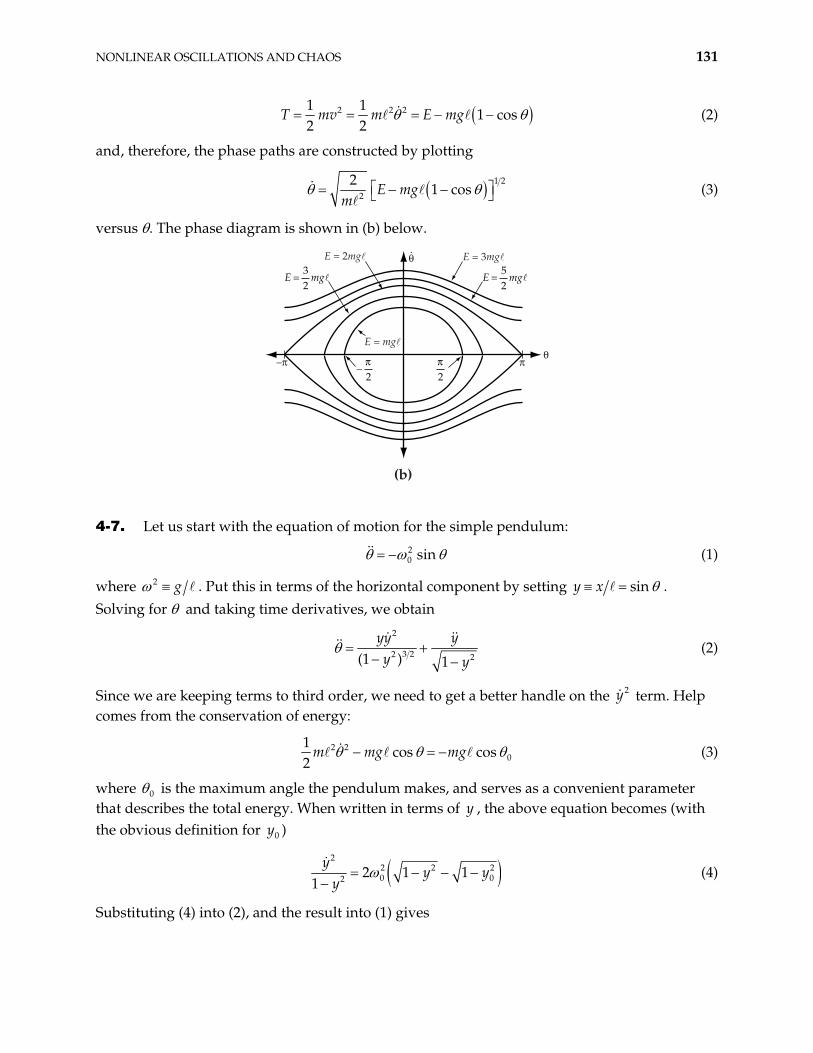
NONLINEAR OSCILLATIONS AND CHAOS 131
2 2 21 11 cos
2 2v m E mgT m (2)
and, therefore, the phase paths are constructed by plotting
1 2
2
21 cosE mg
m (3)
versus . The phase diagram is shown in (b) below.
E = 2mg! E = 3mg!
E = mg!!
·!
–" "# "2
"2
E mg= 32
! E mg= 52
!
(b)
4-7. Let us start with the equation of motion for the simple pendulum:
20 sin (1)
where 2 g . Put this in terms of the horizontal component by setting siny x . Solving for and taking time derivatives, we obtain
2
3 22 2(1 ) 1
yy yy y
(2)
Since we are keeping terms to third order, we need to get a better handle on the term. Help comes from the conservation of energy:
2y
2 20
1cos cos
2m mg mg (3)
where 0 is the maximum angle the pendulum makes, and serves as a convenient parameter that describes the total energy. When written in terms of , the above equation becomes (with the obvious definition for )
y
0y
2
2 202 2 1 1
1y
yy
20y (4)
Substituting (4) into (2), and the result into (1) gives
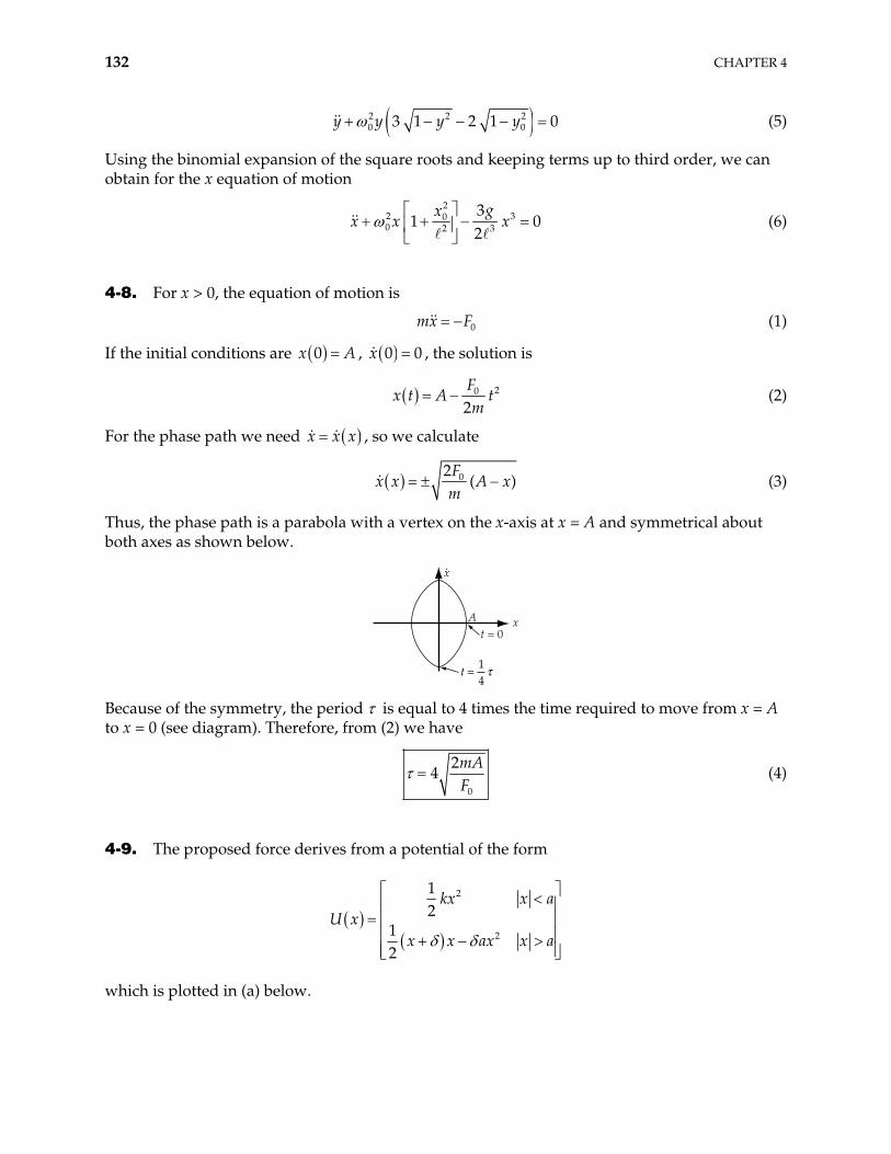
132 CHAPTER 4
2 2 20 3 1 2 1 0y y y y0 (5)
Using the binomial expansion of the square roots and keeping terms up to third order, we can obtain for the x equation of motion
2
2 00 2 3
31
2gx
x x x3 0 (6)
4-8. For x > 0, the equation of motion is
0mx F (1)
If the initial conditions are 0x A , 0x 0 , the solution is
20
2F
x t A tm
(2)
For the phase path we need x x x , so we calculate
02(
Fx x A x
m) (3)
Thus, the phase path is a parabola with a vertex on the x-axis at x = A and symmetrical about both axes as shown below.
t = 0
·x
A x
t = 14
"
Because of the symmetry, the period is equal to 4 times the time required to move from x = A to x = 0 (see diagram). Therefore, from (2) we have
0
24
mAF
(4)
4-9. The proposed force derives from a potential of the form
2
2
12
12
kx x aU x
x x ax x a
which is plotted in (a) below.
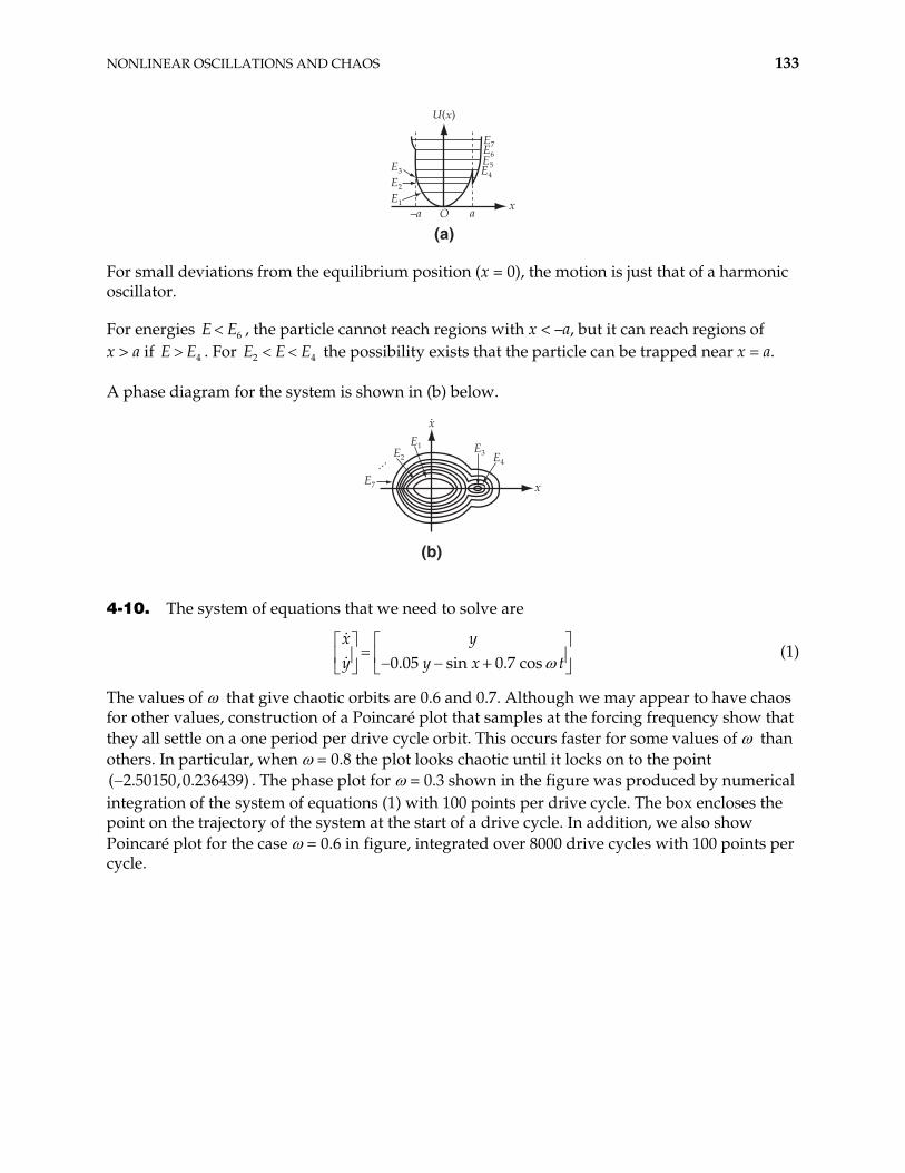
NONLINEAR OSCILLATIONS AND CHAOS 133
U(x)
xa–a O
E3
E2
E1
E7E6E5E4
(a)
For small deviations from the equilibrium position (x = 0), the motion is just that of a harmonic oscillator.
For energies , the particle cannot reach regions with x < –a, but it can reach regions of x > a if . For the possibility exists that the particle can be trapped near x = a.
6E E
4EE 4E E E2
A phase diagram for the system is shown in (b) below.
(b)
·x
x
E1 E3 E4E2
E7
…
4-10. The system of equations that we need to solve are
0.05 sin 0.7 cos
x yy y x t
(1)
The values of that give chaotic orbits are 0.6 and 0.7. Although we may appear to have chaos for other values, construction of a Poincaré plot that samples at the forcing frequency show that they all settle on a one period per drive cycle orbit. This occurs faster for some values of than others. In particular, when = 0.8 the plot looks chaotic until it locks on to the point
. The phase plot for = 0.3 shown in the figure was produced by numerical integration of the system of equations (1) with 100 points per drive cycle. The box encloses the point on the trajectory of the system at the start of a drive cycle. In addition, we also show Poincaré plot for the case = 0.6 in figure, integrated over 8000 drive cycles with 100 points per cycle.
( 2.50150,0.236439)
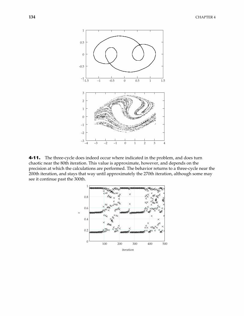
134 CHAPTER 4
–1.5 –1 -0.5 0 0.5 1 1.5–1
-0.5
0
0.5
1
–4–3
–3 –2 –1 0 1 2 3 4
–2
–1
0
1
2
3
4-11. The three-cycle does indeed occur where indicated in the problem, and does turn chaotic near the 80th iteration. This value is approximate, however, and depends on the precision at which the calculations are performed. The behavior returns to a three-cycle near the 200th iteration, and stays that way until approximately the 270th iteration, although some may see it continue past the 300th.
100 200 300 400 5000
0.2
0.4
0.6
0.8
1
x
iteration
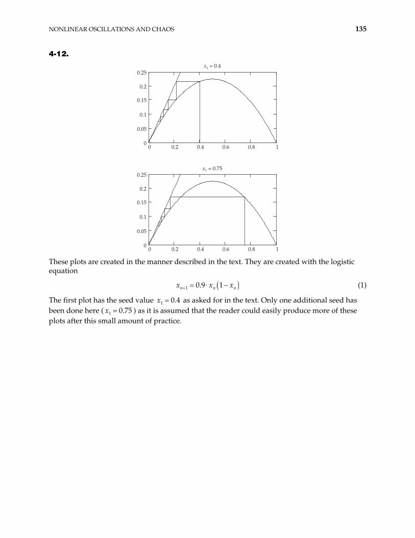
NONLINEAR OSCILLATIONS AND CHAOS 135
4-12.
0 0.2 0.4 0.6 0.8 10
0.1
0.05
0.2
0.25
0.15
x1 = 0.4
x1 = 0.75
0 0.2 0.4 0.6 0.8 10
0.1
0.2
0.05
0.25
0.15
These plots are created in the manner described in the text. They are created with the logistic equation
1 0.9 1n nx x nx (1)
The first plot has the seed value as asked for in the text. Only one additional seed has been done here ( ) as it is assumed that the reader could easily produce more of these plots after this small amount of practice.
1 0.4x
1 0.75x
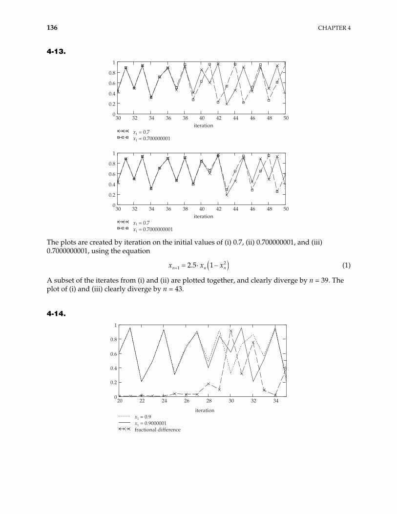
136 CHAPTER 4
4-13.
30 32 34 36 38 40 42 44 46 48 500
0.2
0.4
0.6
0.8
1
x1 = 0.7x1 = 0.700000001
iteration
30 32 34 36 38 40 42 44 46 48 500
1
x1 = 0.7x1 = 0.7000000001
iteration
0.2
0.4
0.6
0.8
The plots are created by iteration on the initial values of (i) 0.7, (ii) 0.700000001, and (iii) 0.7000000001, using the equation
21 2.5 1n nx x nx (1)
A subset of the iterates from (i) and (ii) are plotted together, and clearly diverge by n = 39. The plot of (i) and (iii) clearly diverge by n = 43.
4-14.
20 22 24 26 28 30 32 340
0.2
0.4
0.6
0.8
1
x1 = 0.9x1 = 0.9000001fractional difference
iteration
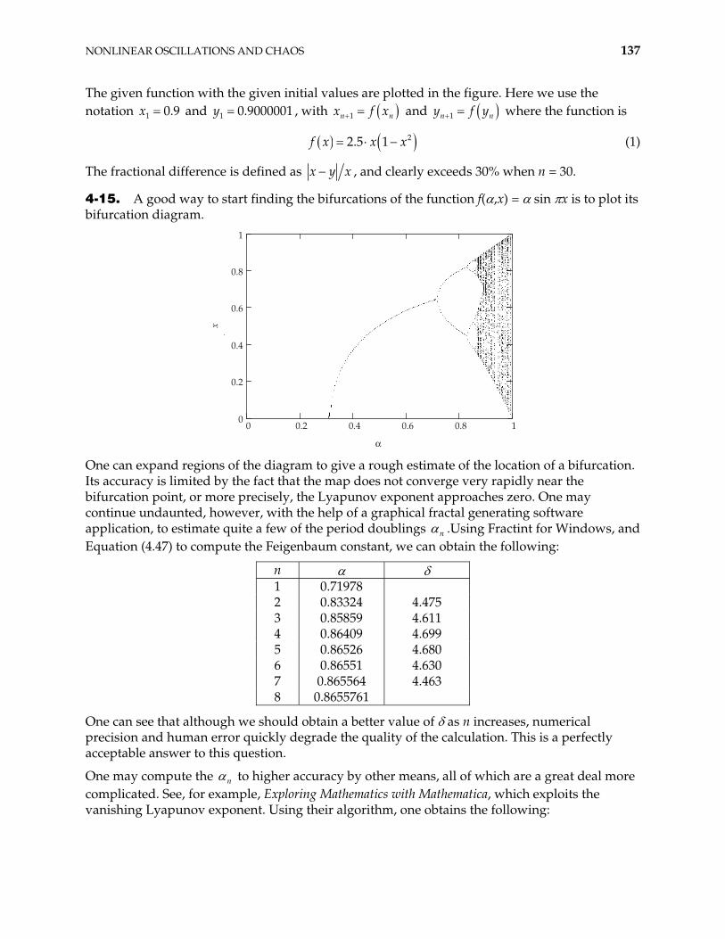
NONLINEAR OSCILLATIONS AND CHAOS 137
The given function with the given initial values are plotted in the figure. Here we use the notation and , with 1 0.9x 1 0.9000001y 1n nx f x and 1ny f yn where the function is
22.5 1f x x x (1)
The fractional difference is defined as x y x , and clearly exceeds 30% when n = 30.
4-15. A good way to start finding the bifurcations of the function f( ,x) = sin x is to plot its bifurcation diagram.
0 0.2 0.4 0.6 0.8 10
0.2
0.4
0.6
0.8
1
#
x
One can expand regions of the diagram to give a rough estimate of the location of a bifurcation. Its accuracy is limited by the fact that the map does not converge very rapidly near the bifurcation point, or more precisely, the Lyapunov exponent approaches zero. One may continue undaunted, however, with the help of a graphical fractal generating software application, to estimate quite a few of the period doublings n .Using Fractint for Windows, and Equation (4.47) to compute the Feigenbaum constant, we can obtain the following:
n 1 0.71978 2 0.83324 4.475 3 0.85859 4.611 4 0.86409 4.699 5 0.86526 4.680 6 0.86551 4.630 7 0.865564 4.463 8 0.8655761
One can see that although we should obtain a better value of as n increases, numerical precision and human error quickly degrade the quality of the calculation. This is a perfectly acceptable answer to this question.
One may compute the n to higher accuracy by other means, all of which are a great deal more complicated. See, for example, Exploring Mathematics with Mathematica, which exploits the vanishing Lyapunov exponent. Using their algorithm, one obtains the following:
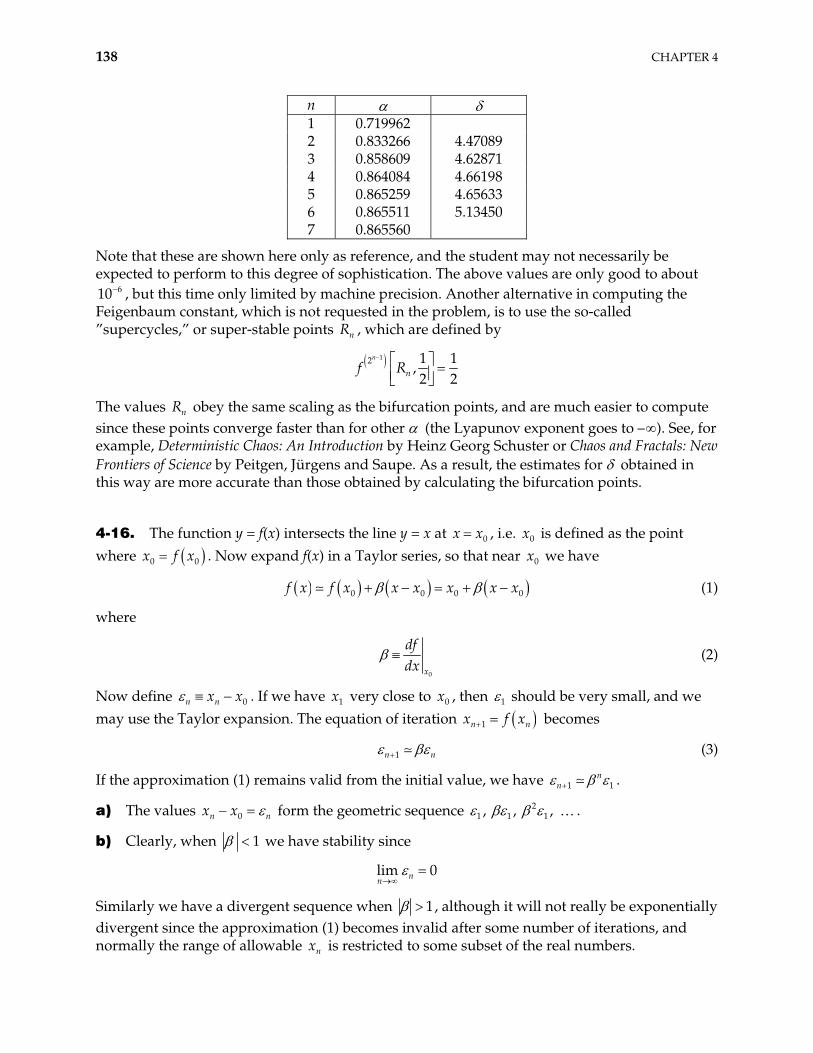
138 CHAPTER 4
n 1 0.719962 2 0.833266 4.47089 3 0.858609 4.62871 4 0.864084 4.66198 5 0.865259 4.65633 6 0.865511 5.13450 7 0.865560
Note that these are shown here only as reference, and the student may not necessarily be expected to perform to this degree of sophistication. The above values are only good to about
, but this time only limited by machine precision. Another alternative in computing the Feigenbaum constant, which is not requested in the problem, is to use the so-called ”supercycles,” or super-stable points , which are defined by
610
nR
12 1 1
,2 2
n
nf R
The values obey the same scaling as the bifurcation points, and are much easier to compute since these points converge faster than for other (the Lyapunov exponent goes to – ). See, for example, Deterministic Chaos: An Introduction by Heinz Georg Schuster or Chaos and Fractals: New Frontiers of Science by Peitgen, Jürgens and Saupe. As a result, the estimates for obtained in this way are more accurate than those obtained by calculating the bifurcation points.
nR
4-16. The function y = f(x) intersects the line y = x at 0x x , i.e. is defined as the point where
0x
0x f x0 . Now expand f(x) in a Taylor series, so that near we have 0x
0 0 0 0f x f x x x x x x (1)
where
0x
dfdx
(2)
Now define 0n nx x . If we have very close to , then 1x 0x 1 should be very small, and we may use the Taylor expansion. The equation of iteration 1 xnx f n
n
becomes
1n (3)
If the approximation (1) remains valid from the initial value, we have 1 1n
n .
a) The values x x0n n form the geometric sequence . 21 1 1, , ,
b) Clearly, when 1 we have stability since
lim 0nn
Similarly we have a divergent sequence when 1, although it will not really be exponentially divergent since the approximation (1) becomes invalid after some number of iterations, and normally the range of allowable is restricted to some subset of the real numbers. nx
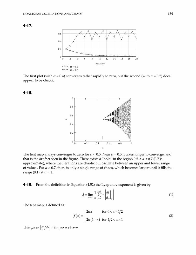
NONLINEAR OSCILLATIONS AND CHAOS 139
4-17.
0 2 4 6 8 10 12 14 16 180
0.2
0.4
0.6
20
# = 0.4# = 0.7
iteration
The first plot (with = 0.4) converges rather rapidly to zero, but the second (with = 0.7) does appear to be chaotic.
4-18.
0 0.2 0.4 0.6 0.8 10
0.2
0.4
0.6
0.8
1
#
x
The tent map always converges to zero for < 0.5. Near = 0.5 it takes longer to converge, and that is the artifact seen in the figure. There exists a “hole” in the region 0.5 < < 0.7 (0.7 is approximate), where the iterations are chaotic but oscillate between an upper and lower range of values. For > 0.7, there is only a single range of chaos, which becomes larger until it fills the range (0,1) at = 1.
4-19. From the definition in Equation (4.52) the Lyapunov exponent is given by
1
0
1lim ln
i
n
ni x
dfn dx
(1)
The tent map is defined as
2 for 0
2 1 for 1 2 1
x xf x
x x
1 2 (2)
This gives 2df dx , so we have
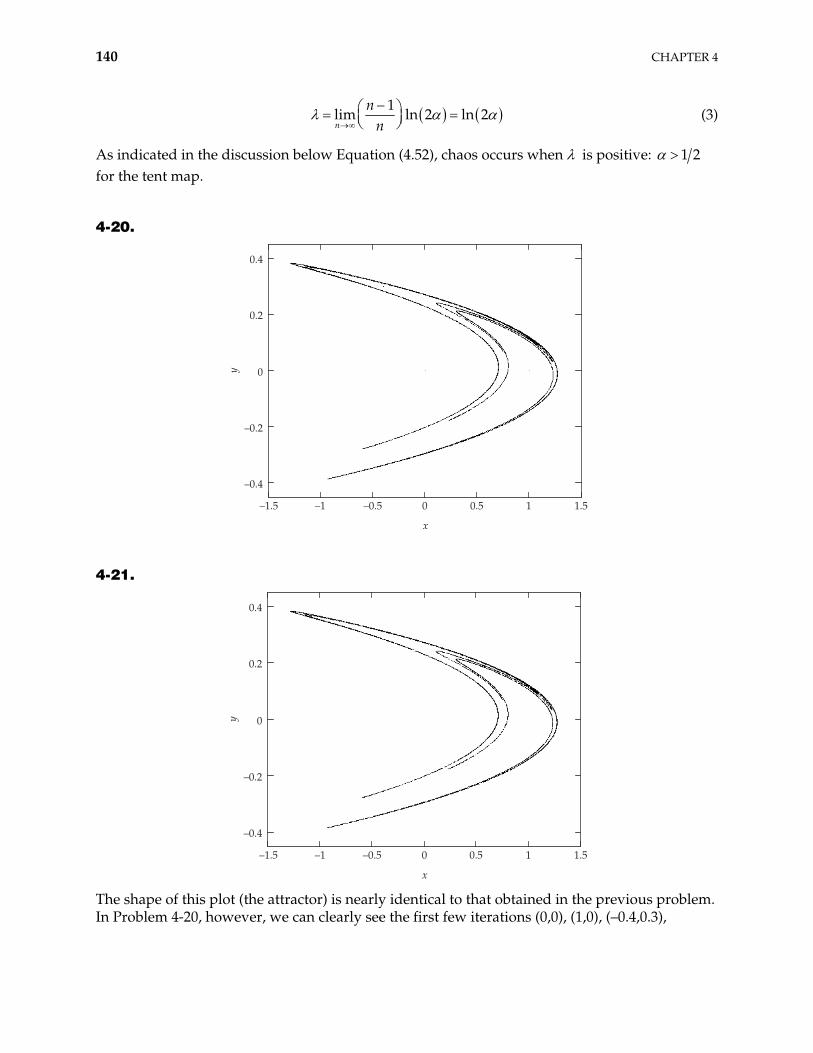
140 CHAPTER 4
1
lim ln 2 ln 2n
nn
(3)
As indicated in the discussion below Equation (4.52), chaos occurs when is positive: 1 2 for the tent map.
4-20.
–1.5 –1 –0.5 0 0.5 1 1.5
–0.4
–0.2
0
0.2
0.4
x
y
4-21.
–1.5 –1 –0.5 0 0.5 1 1.5
–0.4
–0.2
0
0.2
0.4
x
y
The shape of this plot (the attractor) is nearly identical to that obtained in the previous problem. In Problem 4-20, however, we can clearly see the first few iterations (0,0), (1,0), (–0.4,0.3),
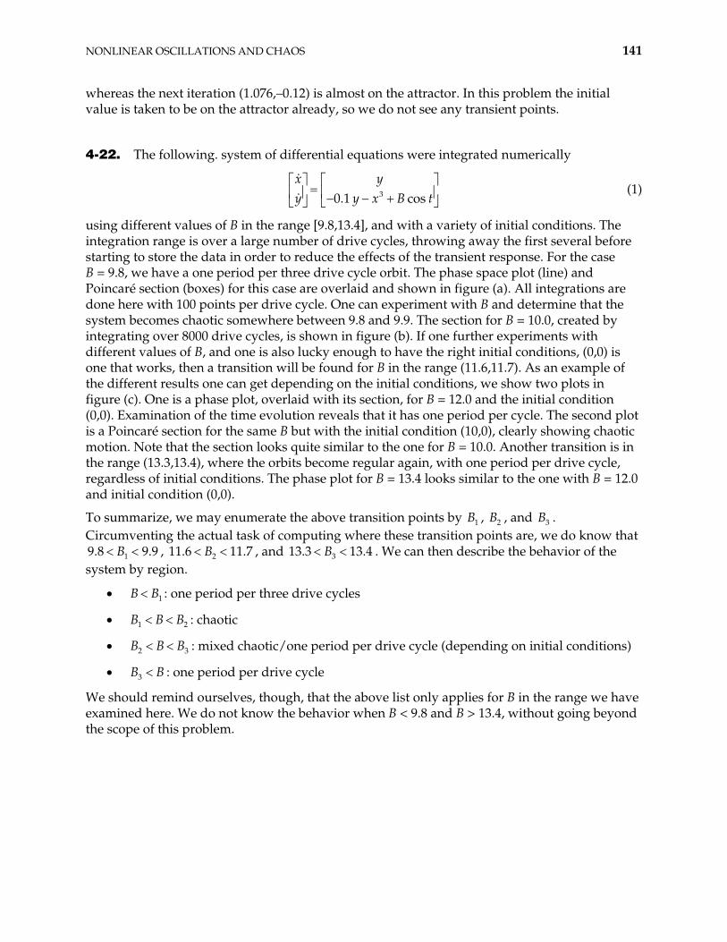
NONLINEAR OSCILLATIONS AND CHAOS 141
whereas the next iteration (1.076,–0.12) is almost on the attractor. In this problem the initial value is taken to be on the attractor already, so we do not see any transient points.
4-22. The following. system of differential equations were integrated numerically
(1) 30.1 cosx yy y x B t
using different values of B in the range [9.8,13.4], and with a variety of initial conditions. The integration range is over a large number of drive cycles, throwing away the first several before starting to store the data in order to reduce the effects of the transient response. For the case B = 9.8, we have a one period per three drive cycle orbit. The phase space plot (line) and Poincaré section (boxes) for this case are overlaid and shown in figure (a). All integrations are done here with 100 points per drive cycle. One can experiment with B and determine that the system becomes chaotic somewhere between 9.8 and 9.9. The section for B = 10.0, created by integrating over 8000 drive cycles, is shown in figure (b). If one further experiments with different values of B, and one is also lucky enough to have the right initial conditions, (0,0) is one that works, then a transition will be found for B in the range (11.6,11.7). As an example of the different results one can get depending on the initial conditions, we show two plots in figure (c). One is a phase plot, overlaid with its section, for B = 12.0 and the initial condition (0,0). Examination of the time evolution reveals that it has one period per cycle. The second plot is a Poincaré section for the same B but with the initial condition (10,0), clearly showing chaotic motion. Note that the section looks quite similar to the one for B = 10.0. Another transition is in the range (13.3,13.4), where the orbits become regular again, with one period per drive cycle, regardless of initial conditions. The phase plot for B = 13.4 looks similar to the one with B = 12.0 and initial condition (0,0).
To summarize, we may enumerate the above transition points by B , , and . Circumventing the actual task of computing where these transition points are, we do know that
, 11 , and 13.3
1 2B 3B
19.8 9.9B 2.6 11.7B 3 13.4B . We can then describe the behavior of the system by region.
: one period per three drive cycles 1B B
: chaotic 1B B B2
3 : mixed chaotic/one period per drive cycle (depending on initial conditions) 2B B B
: one period per drive cycle 3B B
We should remind ourselves, though, that the above list only applies for B in the range we have examined here. We do not know the behavior when B < 9.8 and B > 13.4, without going beyond the scope of this problem.
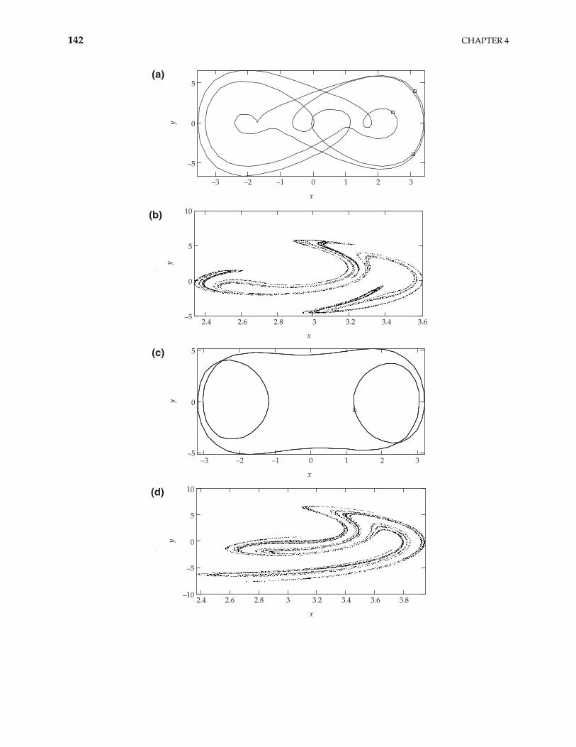
142 CHAPTER 4
–3 –2 –1 0 1 2 3
–5
0
5
x
y
(a)
2.4 2.6 2.8 3 3.2 3.4 3.6
–5
0
5
10
x
y
(b)
–3 –2 –1 0 1 2 3
–5
0
5
x
y
(c)
2.4 2.6 2.8 3 3.2 3.4 3.6 3.8
–10
–5
0
5
10
x
y
(d)
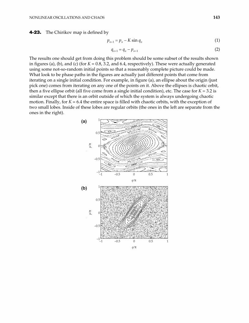
NONLINEAR OSCILLATIONS AND CHAOS 143
4-23. The Chirikov map is defined by
1 sinn np p K nq (1)
1n n nq q p 1 (2)
The results one should get from doing this problem should be some subset of the results shown in figures (a), (b), and (c) (for K = 0.8, 3.2, and 6.4, respectively). These were actually generated using some not-so-random initial points so that a reasonably complete picture could be made. What look to be phase paths in the figures are actually just different points that come from iterating on a single initial condition. For example, in figure (a), an ellipse about the origin (just pick one) comes from iterating on any one of the points on it. Above the ellipses is chaotic orbit, then a five ellipse orbit (all five come from a single initial condition), etc. The case for K = 3.2 is similar except that there is an orbit outside of which the system is always undergoing chaotic motion. Finally, for K = 6.4 the entire space is filled with chaotic orbits, with the exception of two small lobes. Inside of these lobes are regular orbits (the ones in the left are separate from the ones in the right).
–1 –0.5 0 0.5 1
–1
–0.5
0
0.5
1
q ⁄!
p⁄!
(a)
–1 –0.5 0 0.5 1
–1
–0.5
0
0.5
1
q ⁄!
p⁄!
(b)
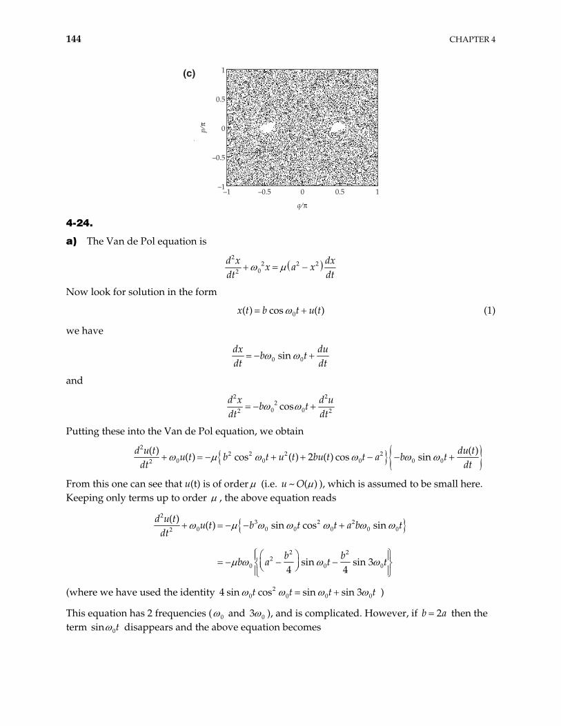
144 CHAPTER 4
–1 –0.5 0 0.5 1–1
–0.5
0
0.5
1
q ⁄!p⁄
!
(c)
4-24.
a) The Van de Pol equation is
2
2 2 202
d x dxx a x
dt dt
Now look for solution in the form
0( ) cos ( )x t b t u t (1)
we have
0 0sindx du
b tdt dt
and
2 2
20 02 2cos
d x d ub t
dt dt
Putting these into the Van de Pol equation, we obtain
2
2 2 2 20 0 0 0 02
( ) ( )( ) cos ( ) 2 ( ) cos sin
d u t du tu t b t u t bu t t a b t
dt dt
From this one can see that u(t) is of order (i.e. ~ ( )u O ), which is assumed to be small here. Keeping only terms up to order , the above equation reads
23 2 2
0 0 0 0 02
2 22
0 0
( )( ) sin cos sin
sin sin 34 4
d u tu t b t t a b t
dt
b bb a t t
0
0
0t
(where we have used the identity 20 0 04 sin cos sin sin 3t t t )
This equation has 2 frequencies ( 0 and 3 0 ), and is complicated. However, if then the term
2b a
0sin t disappears and the above equation becomes
NONLINEAR OSCILLATIONS AND CHAOS 145
2 3
0 02
( )( ) sin 3
4d u t b
u t tdt 0
We let , and the solution for this equation is 2b a
3 3
0 00 0
( ) sin 3 sin 332 4
b at tu t
So, finally putting this form of u(t) into (1), we obtain one of the exact solutions of Van de Pol equation:
3
0 00
( ) 2 cos sin 34
au t a t t
b) See phase diagram below. Since 0.05 is very small, then actually the second term in the expression of u(t) is negligible, and the phase diagram is very close to a circle of radius b = 2a = 2.
x
–2
–1
1
2
.x
–2 –1 1 2
4-25. We have used Mathematica to numerically solve and plot the phase diagram for the van de Pol equation. Because 0.07 is a very small value, the limit cycle is very close to a circle of radius b = 2a = 2.
a) In this case, see figure a), the phase diagram starts at the point (x = 1, x = 0) inside the limit cycle, so the phase diagram spirals outward to ultimately approach the stable solution presented by the limit cycle (see problem 4-24 for exact expression of stable solution).
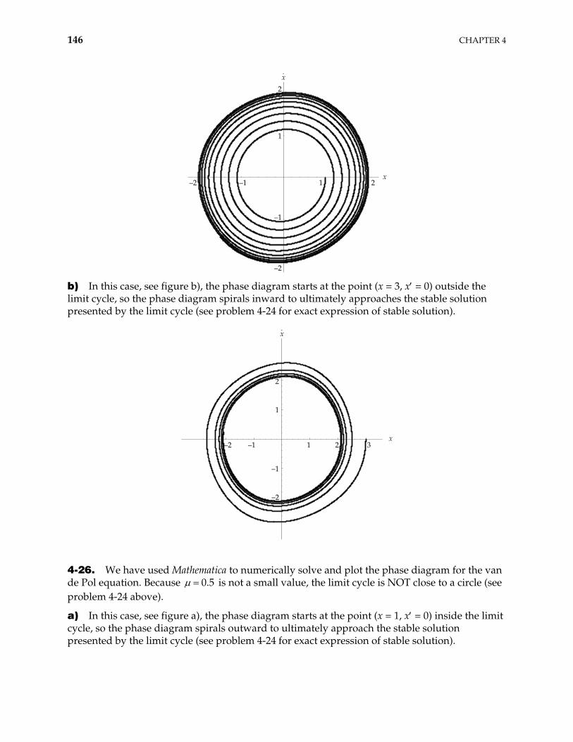
146 CHAPTER 4
x
.x
–2 –1 1 2
–2
–1
1
2
–2 –1 1 2 3
–2
–1
1
2
b) In this case, see figure b), the phase diagram starts at the point (x = 3, x = 0) outside the limit cycle, so the phase diagram spirals inward to ultimately approaches the stable solution presented by the limit cycle (see problem 4-24 for exact expression of stable solution).
x
.x
4-26. We have used Mathematica to numerically solve and plot the phase diagram for the van de Pol equation. Because 0.5 is not a small value, the limit cycle is NOT close to a circle (see problem 4-24 above).
a) In this case, see figure a), the phase diagram starts at the point (x = 1, x = 0) inside the limit cycle, so the phase diagram spirals outward to ultimately approach the stable solution presented by the limit cycle (see problem 4-24 for exact expression of stable solution).
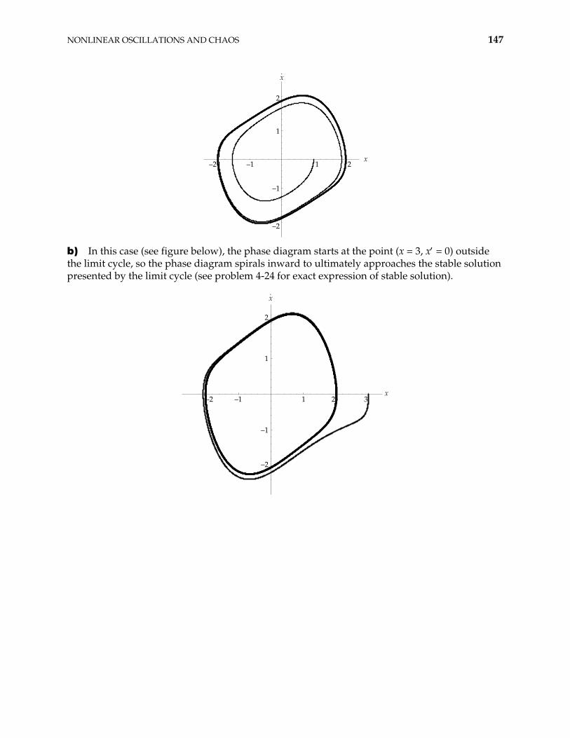
NONLINEAR OSCILLATIONS AND CHAOS 147
x
.x
–2 –1 1 2
–2
–1
1
2
–2 –1 1 2 3
–2
–1
1
2
b) In this case (see figure below), the phase diagram starts at the point (x = 3, x = 0) outside the limit cycle, so the phase diagram spirals inward to ultimately approaches the stable solution presented by the limit cycle (see problem 4-24 for exact expression of stable solution).
x
.x

148 CHAPTER 4
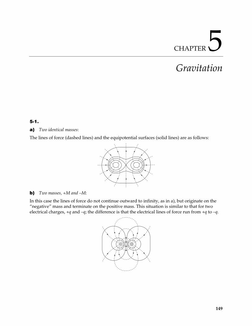
CHAPTER 5 Gravitation
5-1.
a) Two identical masses:
The lines of force (dashed lines) and the equipotential surfaces (solid lines) are as follows:
b) Two masses, +M and –M:
In this case the lines of force do not continue outward to infinity, as in a), but originate on the “negative” mass and terminate on the positive mass. This situation is similar to that for two electrical charges, +q and –q; the difference is that the electrical lines of force run from +q to –q.
149
150 CHAPTER 5
5-2. Inside the sphere the gravitational potential satisfies
2 4 G r (1)
Since (r) is spherically symmetric, is also spherically symmetric. Thus,
22
14r G
r r rr (2)
The field vector is independent of the radial distance. This fact implies
r
= constant C (3)
Therefore, (2) becomes
2
4C
Gr
(4)
or,
2
CGr
(5)
5-3. In order to remove a particle from the surface of the Earth and transport it infinitely far away, the initial kinetic energy must equal the work required to move the particle from er R to r = against the attractive gravitational force:
202
12e
e
R
M mG dr m
rv (1)
where eM and are the mass and the radius of the Earth, respectively, and is the initial velocity of the particle at .
eR 0v
er R
Solving (1), we have the expression for : 0v
02 e
e
G Mv
R (2)
Substituting G , , , we have 11 3 26.67 10 m /kg s 245.98 10 kgeM 66.38 10 meR
0 11.2 km/secv (3)
5-4. The potential energy corresponding to the force is
2
23 2
dx mkU F dx mk
x x2 (1)
The central force is conservative and so the total energy is constant and equal to the potential energy at the initial position, x = d:
GRAVITATION 151
2 2
22
1 1 1constant
2 2 2k
x mx d2
kmE m (2)
Rewriting this equation in integrable form,
0 0
2 22
2 21 1d d
dx d xdx
k d xkx d
dt (3)
where the choice of the negative sign for the radical insures that x decreases as t increases. Using Eq. (E.9), Appendix E, we find
0
2 2
d
dt d x
k (4)
or
2d
tk
5-5. The equation of motion is
2
Mmmx G
x (1)
Using conservation of energy, we find
21 12
x G M E G Mx x
1 (2)
1 1
2dx
GMdt x x
(3)
where is some fixed large distance. Therefore, the time for the particle to travel from x x to x is
1
21 12
x x
x x
xxdxx xGM
GMx x
t d x
Making the change of variable, , and using Eq. (E.7), Appendix E, we obtain 2x y
1sin2
x
x
x xx x x
GM xt x (4)
If we set x = 0 and 2x x in (4), we can obtain the time for the particle to travel the total distance and the first half of the distance.
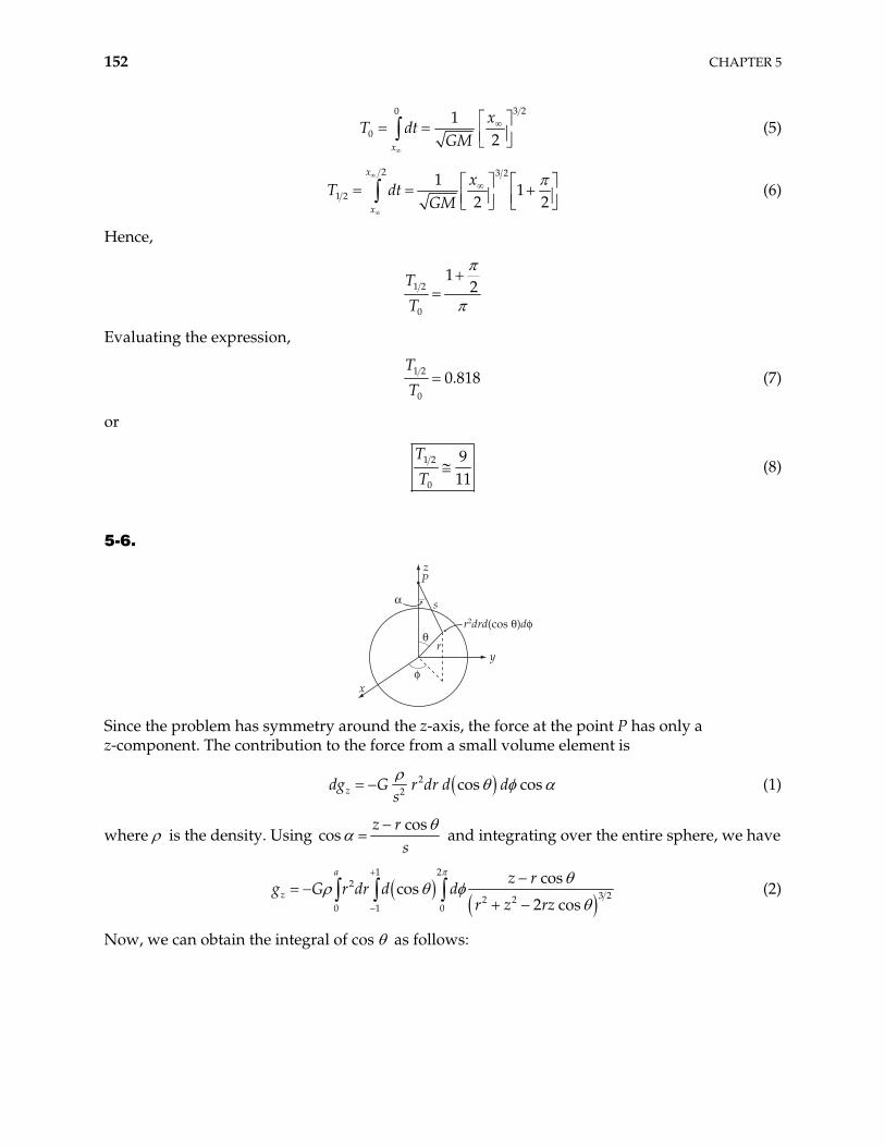
152 CHAPTER 5
3 20
01
2x
xT dt
GM (5)
2 3 2
1 21
12 2
x
x
xT dt
GM (6)
Hence,
1 2
0
12T
T
Evaluating the expression,
1 2
0
0.818T
T (7)
or
1 2
0
911
T
T (8)
5-6.
!
"
#
z
x
yr
s
P
r2drd(cos ")d#
Since the problem has symmetry around the z-axis, the force at the point P has only a z-component. The contribution to the force from a small volume element is
22 cos coszdg G r dr d d
s (1)
where is the density. Using cos
cosz r
s and integrating over the entire sphere, we have
1 2
23 22 2
0 1 0
coscos
2 cos
a
zz r
r dr d dr z rz
g G (2)
Now, we can obtain the integral of cos as follows:
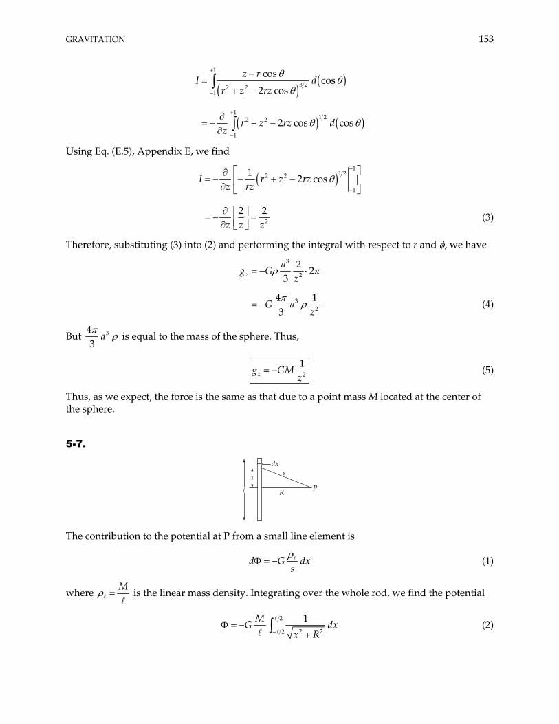
GRAVITATION 153
1
3 22 21
11 22 2
1
coscos
2 cos
2 cos cos
z rI d
r z rz
r z rz dz
Using Eq. (E.5), Appendix E, we find
11 22 2
1
2
12 cos
2 2
I r z rzz rz
z z z (3)
Therefore, substituting (3) into (2) and performing the integral with respect to r and , we have
3
2
32
22
3
4 13
za
g Gz
G az
(4)
But 343
a is equal to the mass of the sphere. Thus,
2
1zg GM
z (5)
Thus, as we expect, the force is the same as that due to a point mass M located at the center of the sphere.
5-7.
dx
PR
sx
The contribution to the potential at P from a small line element is
d Gs
dx (1)
where M
is the linear mass density. Integrating over the whole rod, we find the potential
2
2 22
1MG
x Rdx (2)
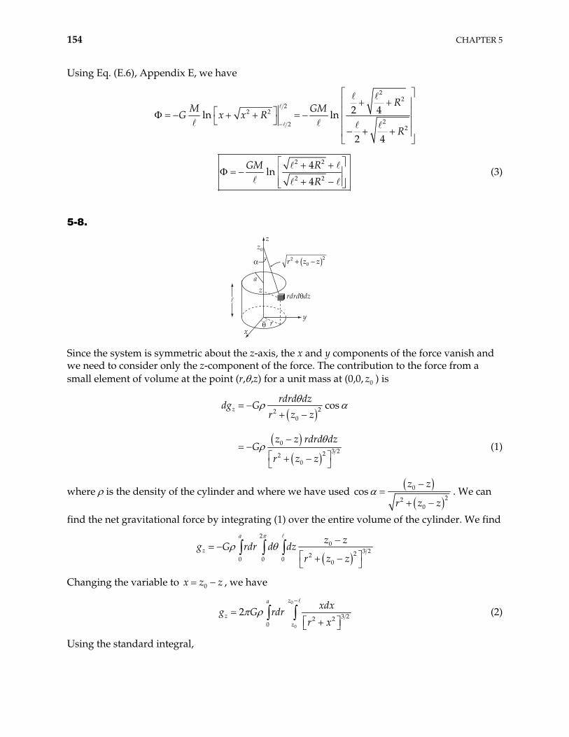
154 CHAPTER 5
Using Eq. (E.6), Appendix E, we have
22
22 2
22 2
2 4ln ln
2 4
RM GMG x x R
R
2 2
2 2
4ln
4
GM R
R (3)
5-8.
z
z
y
xr
a
rdrd"dz
z0
"
! r z z20
2+ $( )
Since the system is symmetric about the z-axis, the x and y components of the force vanish and we need to consider only the z-component of the force. The contribution to the force from a small element of volume at the point (r, ,z) for a unit mass at (0,0, 0z ) is
220
03 222
0
coszrdrd dz
dg Gr z z
z z rdrd dzG
r z z (1)
where is the density of the cylinder and where we have used 0
220
cosz z
r z z. We can
find the net gravitational force by integrating (1) over the entire volume of the cylinder. We find
2
03 2220 0 0 0
a
zz z
rdr d dzr z z
g G
Changing the variable to , we have 0x z z
0
0
3 22 20
2za
zz
xdxg G rdr
r x (2)
Using the standard integral,
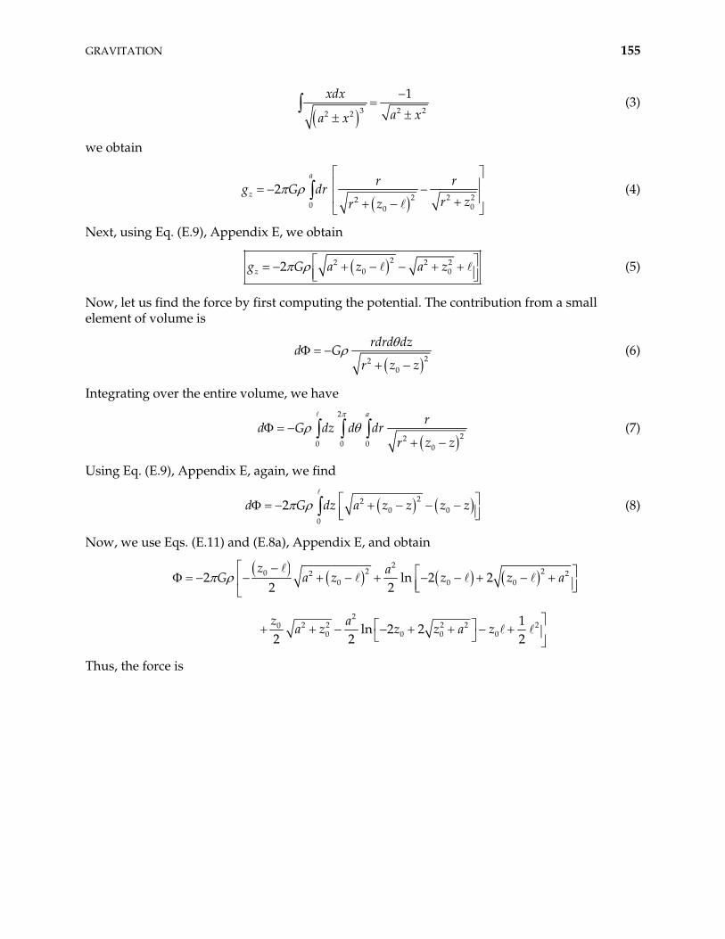
GRAVITATION 155
3 22 2
1xdx
a xa x2
(3)
we obtain
2 2 22
0 00
2a
zr r
drr zr z
g G (4)
Next, using Eq. (E.9), Appendix E, we obtain
22 202z a z a z2
0g G (5)
Now, let us find the force by first computing the potential. The contribution from a small element of volume is
22
0
rdrd dzd G
r z z (6)
Integrating over the entire volume, we have
2
220 0 0 0
a rd G dz d dr
r z z (7)
Using Eq. (E.9), Appendix E, again, we find
220 0
0
2 dz a z z z zd G (8)
Now, we use Eqs. (E.11) and (E.8a), Appendix E, and obtain
22 20 2 2
0 0 0
22 2 2 2 20
0 0 0 0
2 ln 22 2
1ln 2 2
2 2 2
z aG a z z z
z aa z z z a z
2 a
Thus, the force is
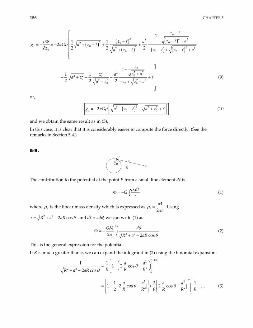
156 CHAPTER 5
022 22
2 0020 2 22 20 0 0 0
02 22 202 2 0
0 2 2 2 20 0 0
11 1
22 2 2
11 12 2 2
z
z
z az ag G a z
z a z z z a
z
z az aa z
a z z z a (9)
or,
22 202z a z a z2
0g G (10
and we obtain the same result as in (5).
In this case, it is clear that it is considerably easier to compute the force directly. (See the remarks in Section 5.4.)
5-9.
"P
r
R
a
The contribution to the potential at the point P from a small line element d is
d
Gr
(1)
where is the linear mass density which is expressed as 2M
a. Using
2 2 2 cosr R a aR and d = ad , we can write (1) as
2
2 202 2 cos
GM d
R a aR (2)
This is the general expression for the potential.
If R is much greater than a, we can expand the integrand in (2) using the binomial expansion:
1 22
22 2
22 2
2 2
1 11 2 cos
2 cos
1 31 2 cos 2 cos
2 8
a aR R RR a aR
a a a aR R R R R
1 (3)
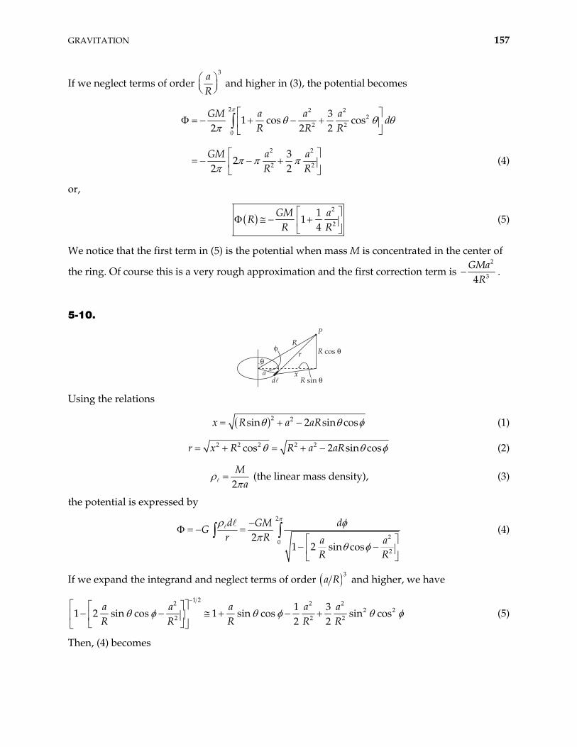
GRAVITATION 157
If we neglect terms of order 3a
R and higher in (3), the potential becomes
2 2 22
2 20
2 2
2 2
31 cos cos
2 2 2
32
2 2
GM a a ad
R R R
GM a aR R
(4)
or,
2
2
11
4GM a
RR R
(5)
We notice that the first term in (5) is the potential when mass M is concentrated in the center of
the ring. Of course this is a very rough approximation and the first correction term is 2
34GMa
R.
5-10.
PR
x
r
aR sin "
R cos ""
#
Using the relations
2 2sin 2 sin cosx R a aR (1)
2 2 2 2 2cos 2 sin cosR R a aRr x (2)
2M
a (the linear mass density), (3)
the potential is expressed by
2
20
2
21 2 sin cos
d GM dG
r R a aR R
(4)
If we expand the integrand and neglect terms of order 3
a R and higher, we have
1 22 22 2
2 2
1 31 2 sin cos 1 sin cos sin cos
2 2a a a a aR R R R R
2
2 (5)
Then, (4) becomes
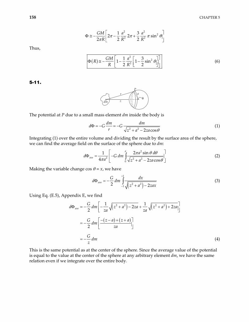
158 CHAPTER 5
2 2
22 2
1 32 2 sin
2 2 2GM a a
R R R
Thus,
2
22
1 31 1 sin
2 2GM a
RR R
(6)
5-11.
Par
zdm"
The potential at P due to a small mass element dm inside the body is
2 2 2 cos
dm dmd G G
r z a za (1)
Integrating (1) over the entire volume and dividing the result by the surface area of the sphere, we can find the average field on the surface of the sphere due to dm:
2
2 2 20
2 sin14 2 cos
avea d
dma z a za
d G (2)
Making the variable change cos = x, we have
1
2 212 2
aveG dx
d dmz a zax
(3)
Using Eq. (E.5), Appendix E, we find
2 2 2 21 12 2
2
2
aveG
d dm z a za z aza za
z a z aGdm
za
Gdm
za
z (4)
This is the same potential as at the center of the sphere. Since the average value of the potential is equal to the value at the center of the sphere at any arbitrary element dm, we have the same relation even if we integrate over the entire body.
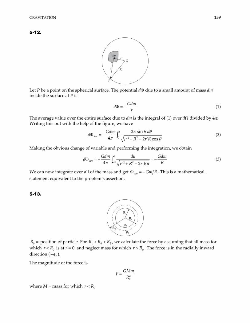
GRAVITATION 159
5-12.
O
P
dm
Rr
r'
Let P be a point on the spherical surface. The potential d due to a small amount of mass dm inside the surface at P is
Gdm
dr
(1)
The average value over the entire surface due to dm is the integral of (1) over d divided by 4 . Writing this out with the help of the figure, we have
20 2
2 sin4 2 cos
avedGdm
R r Rrd (2)
Making the obvious change of variable and performing the integration, we obtain
1
21 24 2ave
Gdm du GdmRR r Rur
d (3)
We can now integrate over all of the mass and get ave Gm R . This is a mathematical statement equivalent to the problem’s assertion.
5-13.
R1
R2
R0
%2
%1
0R position of particle. For , we calculate the force by assuming that all mass for which is at r = 0, and neglect mass for which . The force is in the radially inward direction ( ).
1 0R R R2
0r Re
0r R
r
The magnitude of the force is
20
GMmF
R
where M = mass for which 0r R
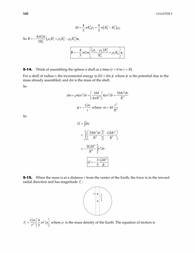
160 CHAPTER 5
3 31 1 0 1 2
4 43 3
M R R R3
So 3 3 31 1 2 0 2 12
0
43 r
GmR R R
RF e
3
1 2 12 02
0
43 r
RGm R
RF e
5-14. Think of assembling the sphere a shell at a time (r = 0 to r = R).
For a shell of radius r, the incremental energy is dU = dm where is the potential due to the mass already assembled, and dm is the mass of the shell.
So
2
2 23 3
3 34 4
4M M
r dr r drR R
r drdm
Gm
r where
3
3
rm M
R
So
2 2
3 30
24
60
3
3
R
r
R
U du
Mr dr GMrR R
GMr dr
R
23
5GM
UR
5-15. When the mass is at a distance r from the center of the Earth, the force is in the inward radial direction and has magnitude rF :
mr
32
43r
GmF
rr where is the mass density of the Earth. The equation of motion is
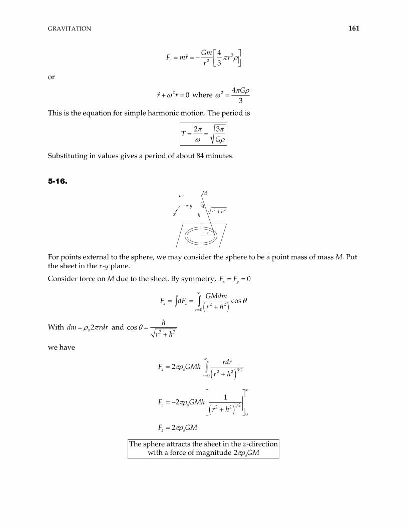
GRAVITATION 161
32
43r
GmF mr r
r
or
where 2 0r r 2 43G
This is the equation for simple harmonic motion. The period is
2 3
TG
Substituting in values gives a period of about 84 minutes.
5-16.
z
y
x
M
h
r
"r h2 2+
For points external to the sphere, we may consider the sphere to be a point mass of mass M. Put the sheet in the x-y plane.
Consider force on M due to the sheet. By symmetry, 0x yF F
2 2
0
cosz zr
GMdmF dF
r h
With 2sdm rdr and 2 2
sh
r hco
we have
3 22 20
1 22 2
0
2
12
2
z sr
z s
z s
rdrF GMh
r h
F GMhr h
F GM
Th
e sphere attracts the sheet in the -direction
with a force of magnitude 2 s
zGM
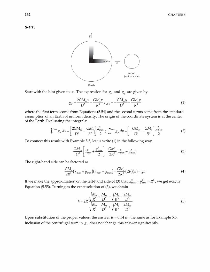
162 CHAPTER 5
5-17.
y
x
Earth
moon(not to scale)
water
Start with the hint given to us. The expression for and xg yg are given by
3 3
2 m ex
GM x GM xD R
g ; 3m
yGM y GM y
gD R3
e (1)
where the first terms come from Equations (5.54) and the second terms come from the standard assumption of an Earth of uniform density. The origin of the coordinate system is at the center of the Earth. Evaluating the integrals:
max2max
3 30
22
x m ex
GM GM xg dx
D R; max
2max
3 30 2y m e
yyGM GM
g dyD R
(2)
To connect this result with Example 5.5, let us write (1) in the following way
2
2 2maxmax max max3 32 2
m ey GMx x
D R2y
GM (3)
The right-hand side can be factored as
max max max max3 22 2
eGM GMx y x y R h g
R R3e h
2R
(4)
If we make the approximation on the left-hand side of (3) that , we get exactly Equation (5.55). Turning to the exact solution of (3), we obtain
2 2max maxx y
3 3 3 3
3 3 3 3
2
22
e m e
e m e
M M M MR D R Dh RM M M MR D R D
m
m
(5)
Upon substitution of the proper values, the answer is 0.54 m, the same as for Example 5.5. Inclusion of the centrifugal term in does not change this answer significantly. xg
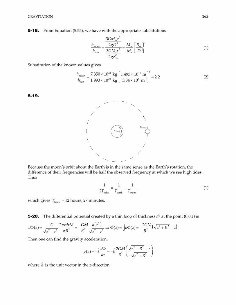
GRAVITATION 163
5-18. From Equation (5.55), we have with the appropriate substitutions
2
33moon
2sun
3
32
32
m
m es
s s
es
GM rgDh M
GM rh MgR
RD
(1)
Substitution of the known values gives
322 11
moon30 8
sun
7 350 10 kg 1 495 10 m2 2
1 993 10 kg 3 84 10 mhh
(2)
5-19.
&earth
&moon
Because the moon’s orbit about the Earth is in the same sense as the Earth’s rotation, the difference of their frequencies will be half the observed frequency at which we see high tides. Thus
tides earth moon
1 1 12T T T
(1)
which gives T 12 hours, 27 minutes. tides
5-20. The differential potential created by a thin loop of thickness dr at the point (0,0,z) is 2
2 22 2 22 2 2 2
2 2( ) ( ) ( )
G rdrM GM d r GMd z z d z z R z
R R Rz r z r
Then one can find the gravity acceleration,
2 2
2 2 2
2ˆ ˆ( )d GM z R
k kdz R z R
zg z
where is the unit vector in the z-direction. k̂
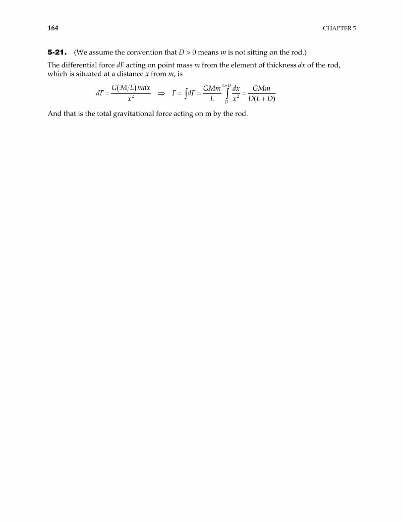
164 CHAPTER 5
5-21. (We assume the convention that D > 0 means m is not sitting on the rod.)
The differential force dF acting on point mass m from the element of thickness dx of the rod, which is situated at a distance x from m, is
2 2 ( )
L D
D
G M L mdx GMm dx GMmdF F dF
x L x D L D
And that is the total gravitational force acting on m by the rod.
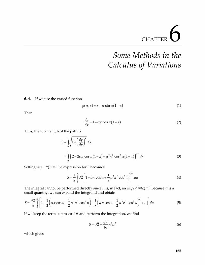
CHAPTER 6 Some Methods in the
Calculus of Variations
6-1. If we use the varied function
, sin 1y x x x (1)
Then
1 cos 1dy
xdx
(2)
Thus, the total length of the path is
21
0
11 22 2 2
0
1
2 cos 1 cos 1
dyS dx
dx
x x2 (3) dx
Setting 1 x u , the expression for S becomes
1 2
2 2 2
0
1 12 1 cos cos
2S u (4) u du
The integral cannot be performed directly since it is, in fact, an elliptic integral. Because is a small quantity, we can expand the integrand and obtain
22 2 2 2 2 2
0
2 1 1 1 11 cos cos cos cos
2 2 8 2S u u u u du (5)
If we keep the terms up to co and perform the integration, we find 2s u
2 222
16S (6)
which gives
165
166 CHAPTER 6
228
S (7)
Therefore
0
0a
S (8)
and S is a minimum when = 0.
6-2. The element of length on a plane is
2dS dx dy2 (1)
from which the total length is
2 2 2
1 1 1
, 22 2
,
1x y x
x y x
dyS dx dy
dxdx (2)
If S is to be minimum, f is identified as
2
1dy
fdx
(3)
Then, the Euler equation becomes
21d d
ydx dy
0 (4)
where dy
ydx
. (4) becomes
2
01
yddx y
(5)
or,
21
y
y = constant C (6)
from which we have
2
21C
yC
= constant a (7)
Then,
y ax b (8)
This is the equation of a straight line.
SOME METHODS IN THE CALCULUS OF VARIATIONS 167
6-3. The element of distance in three-dimensional space is
2 2dS dx dy dz2 (1)
Suppose x, y, z depends on the parameter t and that the end points are expressed by
1 1 1 1 1 1, ,x t y t z t , 2 2 2 2 2 2, ,x t y t z t . Then the total distance is
2
1
22 2t
t
dydx dzS
dt dt dtdt (2)
The function f is identified as
2 2 2f x y z (3)
Since 0f f fx y z
, the Euler equations become
0
0
0
fddt x
fddt y
fddt z
(4)
from which we have
12 2 2
22 2 2
32 2 2
constant
constant
constant
xC
x y z
yC
x y z
zC
x y z
(5)
From the combination of these equations, we have
1 2
2 3
yxC C
y zC C
(6)
If we integrate (6) from t to the arbitrary t, we have 1
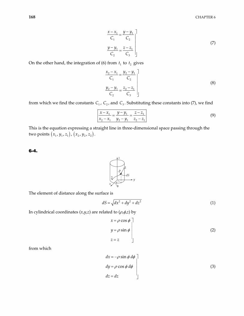
168 CHAPTER 6
11
1 2
1 1
2 3
y yx xC C
y y z zC C
(7)
On the other hand, the integration of (6) from to gives 1t 2t
2 12 1
1 2
2 1 2 1
2 3
y yx xC C
y y z zC C
(8)
from which we find the constants , C , and C . Substituting these constants into (7), we find 1C 2 3
11
2 1 2 1 2 1
y yx x z zx x y y z z
1 (9)
This is the equation expressing a straight line in three-dimensional space passing through the two points 1 1 1, ,x y z , 2 2 2, ,x y z .
6-4.
x
y
z
1
2dS
!
"
The element of distance along the surface is
2 2dS dx dy dz2 (1)
In cylindrical coordinates (x,y,z) are related to ( , ,z) by
cos
sin
x
y
z z
(2)
from which
sin
cos
dx d
dy d
dz dz
(3)
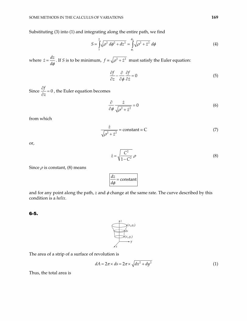
SOME METHODS IN THE CALCULUS OF VARIATIONS 169
Substituting (3) into (1) and integrating along the entire path, we find
2
1
22 2 2 2 2
1
S d dz z d (4)
where dz
zd
. If S is to be minimum, 2 2f z must satisfy the Euler equation:
0f fz z
(5)
Since 0fz
, the Euler equation becomes
2 2
0z
z (6)
from which
2 2
z
z= constant C (7)
or,
2
21C
zC
(8)
Since is constant, (8) means
constantdzd
and for any point along the path, z and change at the same rate. The curve described by this condition is a helix.
6-5.
ds
(x1,y1)
(x2,y2)
y
x
z
The area of a strip of a surface of revolution is
22 2dA ds dx dy2 (1)
Thus, the total area is
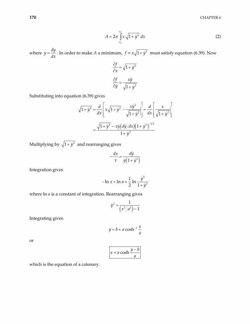
170 CHAPTER 6
2
1
22 1x
x
A x y dx (2)
where dy
ydx
. In order to make A a minimum, 21f x y must satisfy equation (6.39). Now
2
2
1
1
fy
x
f xyy y
Substituting into equation (6.39) gives
22 2
2 2
1 22 2
2
1 11 1
1 1
1
xyd dy x y
dx dxy y
y xy dy dx y
y
x
Multiplying by 21 y and rearranging gives
21
dydxx y y
Integration gives
2
2
1ln ln ln
2 1y
x ay
where ln a is a constant of integration. Rearranging gives
22 2
11
yx a
Integrating gives
1coshx
y b aa
or
coshy b
x aa
which is the equation of a catenary.
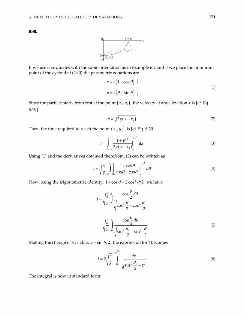
SOME METHODS IN THE CALCULUS OF VARIATIONS 171
6-6.
(x1,y1)
(x2,y2)2a
0
# = 0
# = $
x
y
If we use coordinates with the same orientation as in Example 6.2 and if we place the minimum point of the cycloid at (2a,0) the parametric equations are
1 cos
sin
x a
y a (1)
Since the particle starts from rest at the point 1 1,x y , the velocity at any elevation x is [cf. Eq. 6.19]
12v g x x (2)
Then, the time required to reach the point 2 2,x y is [cf. Eq. 6.20]
2
1
1 22
1
12
x
x
yt
g x xdx (3)
Using (1) and the derivatives obtained therefrom, (3) can be written as
1
2
1 2
10
1 coscos cos
at
gd (4)
Now, using the trigonometric identity, 2cos 2 cos 21 , we have
1
1
2 2 10
2 210
cos2
cos cos2 2
cos2
sin sin2 2
dat
g
dag
(5)
Making the change of variable, sin 2z , the expression for t becomes
1sin2
2 210
2sin
2
a dzt
gz
(6)
The integral is now in standard form:
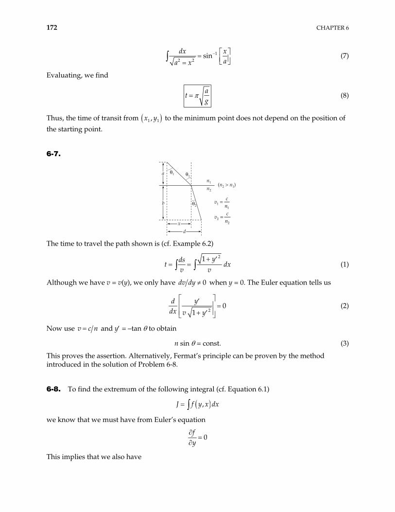
172 CHAPTER 6
1
2 2sin
dx xaa x
(7)
Evaluating, we find
a
tg
(8)
Thus, the time of transit from 1 1,x y to the minimum point does not depend on the position of the starting point.
6-7.
vcn1
1
=
vc
n22
=
n1
n2
#1 #1
#2
(n2 > n1)
d
b
x
a
The time to travel the path shown is (cf. Example 6.2)
21 yds
tv v
dx (1)
Although we have v = v(y), we only have 0dv dy when y = 0. The Euler equation tells us
2
01
yddx v y
(2)
Now use v c n and y = –tan to obtain
n sin = const. (3)
This proves the assertion. Alternatively, Fermat’s principle can be proven by the method introduced in the solution of Problem 6-8.
6-8. To find the extremum of the following integral (cf. Equation 6.1)
,J f y x dx
we know that we must have from Euler’s equation
0fy
This implies that we also have
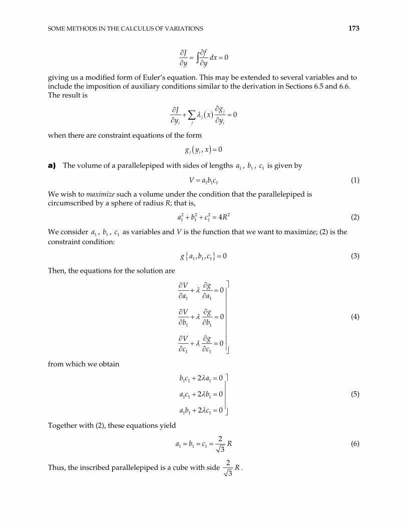
SOME METHODS IN THE CALCULUS OF VARIATIONS 173
0fJ
dxy y
giving us a modified form of Euler’s equation. This may be extended to several variables and to include the imposition of auxiliary conditions similar to the derivation in Sections 6.5 and 6.6. The result is
0jj
ji i
gJx
y y
when there are constraint equations of the form
, 0j ig y x
a) The volume of a parallelepiped with sides of lengths , b , is given by 1a 1 1c
1 1 1V a b c (1)
We wish to maximize such a volume under the condition that the parallelepiped is circumscribed by a sphere of radius R; that is,
(2) 2 2 21 1 1 4a b c R2
We consider , , c as variables and V is the function that we want to maximize; (2) is the constraint condition:
1a 1b 1
1 1 1, , 0g a b c (3)
Then, the equations for the solution are
1 1
1 1
1 1
0
0
0
gVa a
gVb b
gVc c
(4)
from which we obtain
1 1 1
1 1 1
1 1 1
2 0
2 0
2 0
b c a
a c b
a b c
(5)
Together with (2), these equations yield
1 1 123
a b c R (6)
Thus, the inscribed parallelepiped is a cube with side 23
R .
174 CHAPTER 6
b) In the same way, if the parallelepiped is now circumscribed by an ellipsoid with semiaxes a, b, c, the constraint condition is given by
2 2 21 1 1
2 2 2 14 4 4a b ca b z
(7)
where , , c are the lengths of the sides of the parallelepiped. Combining (7) with (1) and (4) gives
1a 1b 1
2 21 12 2
a b ca b c
212 (8)
Then,
1 1 12 2
, ,3 3
a a b b c c23
(9)
6-9. The average value of the square of the gradient of 1 2 3, ,x x x within a certain volume V is expressed as
21 2 3
22 2
1 21 2 3
1
1
I dx dx dxV
V x x x 3dx dx dxv (1)
In order to make I a minimum,
22 2
1 2
fx x x3
must satisfy the Euler equation:
3
1
0i i
i
f fx
x
(2)
If we substitute f into (2), we have
3
1
0i i ix x
(3)
which is just Laplace’sequation:
2 0 (4)
Therefore, must satisfy Laplace’s equation in order that I have a minimum value.
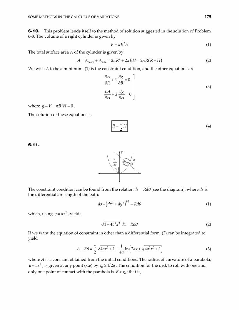
SOME METHODS IN THE CALCULUS OF VARIATIONS 175
6-10. This problem lends itself to the method of solution suggested in the solution of Problem 6-8. The volume of a right cylinder is given by
(1) 2V R H
The total surface area A of the cylinder is given by
2bases side 2 2 2A A A R RH R R H (2)
We wish A to be a minimum. (1) is the constraint condition, and the other equations are
0
0
gAR R
gAH H
(3)
where . 2 0g V R H
The solution of these equations is
12
R H (4)
6-11.
y
dsR#
}12a
The constraint condition can be found from the relation ds = Rd (see the diagram), where ds is the differential arc length of the path:
1 22 2ds dx dy Rd (1)
which, using , yields 2y ax
2 21 4a x dx Rd (2)
If we want the equation of constraint in other than a differential form, (2) can be integrated to yield
2 14 1 ln 2 4
2 4x
ax ax a xa
2 2 1A R (3)
where A is a constant obtained from the initial conditions. The radius of curvature of a parabola, , is given at any point (x,y) by 2y ax 0 1 2r . The condition for the disk to roll with one and
only one point of contact with the parabola is a
0R r ; that is,
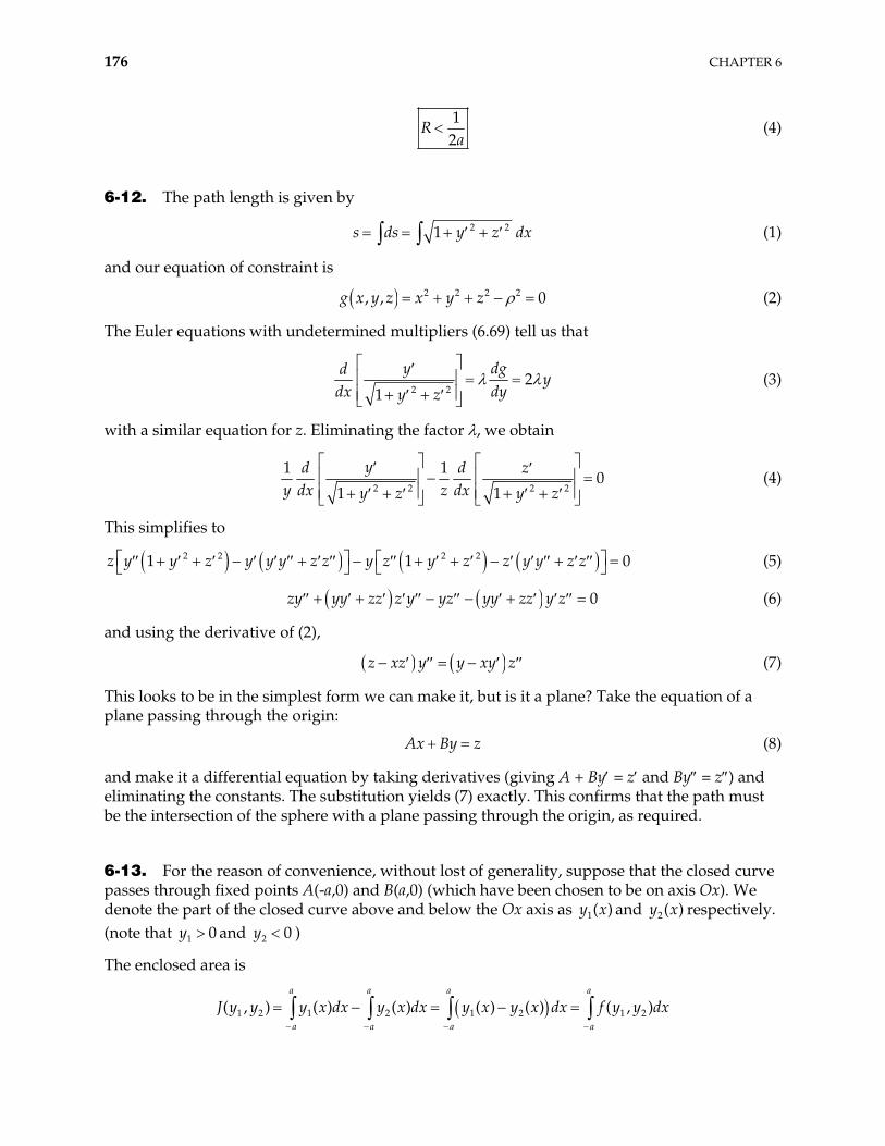
176 CHAPTER 6
12
Ra
(4)
6-12. The path length is given by
2 21s ds y z dx (1)
and our equation of constraint is
2 2 2 2, , 0g x y z x y z (2)
The Euler equations with undetermined multipliers (6.69) tell us that
2 2
21
y dgdy
dx dyy z (3)
with a similar equation for z. Eliminating the factor , we obtain
2 2 2 2
01 1
yd d zy dx z dxy z y z
1 1 (4)
This simplifies to
2 2 2 21 1z y y z y y y z z y z y z z y y z z 0 (5)
0yy zz z y yz yy zz y zzy (6)
and using the derivative of (2),
z xz y y xy z (7)
This looks to be in the simplest form we can make it, but is it a plane? Take the equation of a plane passing through the origin:
Ax By z (8)
and make it a differential equation by taking derivatives (giving A + By = z and By = z ) and eliminating the constants. The substitution yields (7) exactly. This confirms that the path must be the intersection of the sphere with a plane passing through the origin, as required.
6-13. For the reason of convenience, without lost of generality, suppose that the closed curve passes through fixed points A(-a,0) and B(a,0) (which have been chosen to be on axis Ox). We denote the part of the closed curve above and below the Ox axis as and respectively. (note that and )
1( )y x 2( )y x
1 0y 2 0y
The enclosed area is
1 2 1 2 1 2 1 2( , ) ( ) ( ) ( ) ( ) ( , )a a a a
a a a a
J y y y x dx y x dx y x y x dx f y y dx
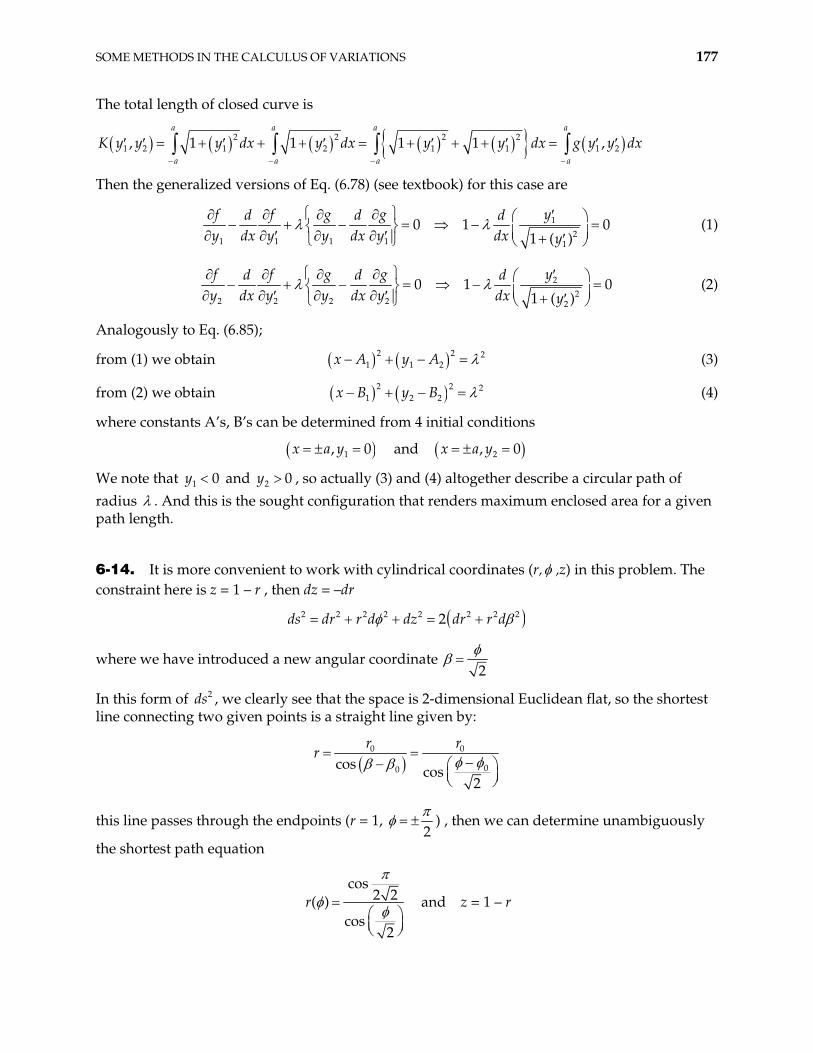
SOME METHODS IN THE CALCULUS OF VARIATIONS 177
The total length of closed curve is
2 2 2 21 2 1 2 1 1 1 2, 1 1 1 1 ,
a a a a
a a a a
K y y y dx y dx y y dx g y y dx
Then the generalized versions of Eq. (6.78) (see textbook) for this case are
12
1 1 1 1 1
0 11 ( )
f f g g yd d dy dx y y dx y dx y
0 (1)
22
2 2 2 2 2
0 11 ( )
f f g g yd d dy dx y y dx y dx y
0 (2)
Analogously to Eq. (6.85);
from (1) we obtain 2 2 21 1 2x A y A (3)
from (2) we obtain 2 2 21 2 2x B y B (4)
where constants A’s, B’s can be determined from 4 initial conditions
1, 0x a y and 2, 0x a y
We note that and , so actually (3) and (4) altogether describe a circular path of radius
1 0y 2 0y. And this is the sought configuration that renders maximum enclosed area for a given
path length.
6-14. It is more convenient to work with cylindrical coordinates (r, ,z) in this problem. The constraint here is z = 1 – r , then dz = –dr
2 2 2 2 2 2 22s dr r d dz dr r d 2d
where we have introduced a new angular coordinate 2
In this form of , we clearly see that the space is 2-dimensional Euclidean flat, so the shortest line connecting two given points is a straight line given by:
2ds
0 0
00cos cos2
r rr
this line passes through the endpoints (r = 1, 2
) , then we can determine unambiguously
the shortest path equation
cos
2 2( )cos
2
r and z = 1 – r
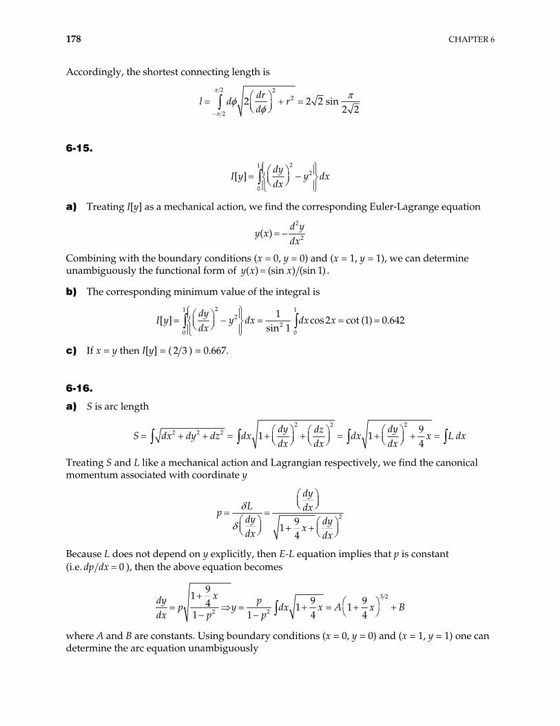
178 CHAPTER 6
Accordingly, the shortest connecting length is
2 2
2
2
2 2 2 sin2 2
drr
dl d
6-15.
21
2
0
[ ]dy
I y y dxdx
a) Treating I[y] as a mechanical action, we find the corresponding Euler-Lagrange equation
2
2( )d y
y xdx
Combining with the boundary conditions (x = 0, y = 0) and (x = 1, y = 1), we can determine unambiguously the functional form of ( ) (sin ) (sin 1)y x x .
b) The corresponding minimum value of the integral is
21 1
22
0 0
1[ ] cos2 cot (1) 0.642
sin 1dy
y dx dx xdx
I y
c) If x = y then I[y] = ( 2 3 ) = 0.667.
6-16.
a) S is arc length
2 22
2 2 2 91 1
4dy dydz
S dx dy dz dx dx x L ddx dx dx
x
Treating S and L like a mechanical action and Lagrangian respectively, we find the canonical momentum associated with coordinate y
2914
dyL dxpdy dy
xdx dx
Because L does not depend on y explicitly, then E-L equation implies that p is constant (i.e. 0dp dx ), then the above equation becomes
3 2
2 2
91 9 94 1 11 1 4 4
xdy pp y dx x A x
dx p pB
where A and B are constants. Using boundary conditions (x = 0, y = 0) and (x = 1, y = 1) one can determine the arc equation unambiguously
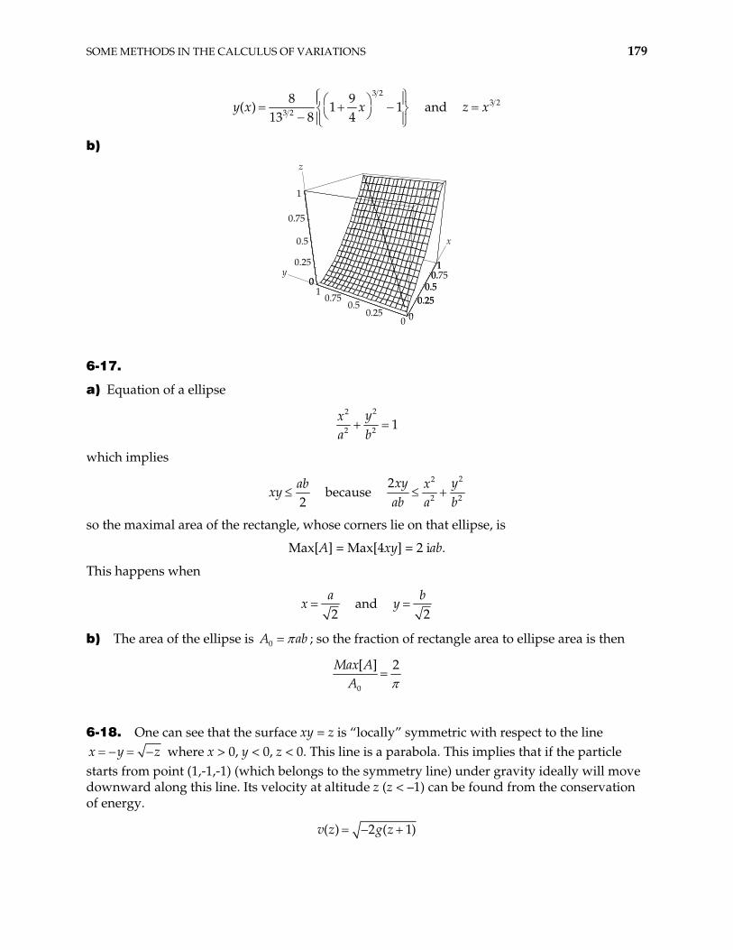
SOME METHODS IN THE CALCULUS OF VARIATIONS 179
3 2
3 28 9
( ) 1 113 8 4
xy x and 3 2z x
b)
z
x
y
0
0.250.5
0.751
00.25
0.50.75
10
0.25
0.5
0.75
1
0
0.250.5
0.1
0
6-17.
a) Equation of a ellipse
22
2 2 1yx
a b
which implies
2ab
xy because 22
2 2
2xy yxab a b
so the maximal area of the rectangle, whose corners lie on that ellipse, is
Max[A] = Max[4xy] = 2 iab.
This happens when
2
ax and
2b
y
b) The area of the ellipse is 0A ab ; so the fraction of rectangle area to ellipse area is then
0
[ ] 2Max AA
6-18. One can see that the surface xy = z is “locally” symmetric with respect to the line x y z where x > 0, y < 0, z < 0. This line is a parabola. This implies that if the particle starts from point (1,-1,-1) (which belongs to the symmetry line) under gravity ideally will move downward along this line. Its velocity at altitude z (z < –1) can be found from the conservation of energy.
( ) 2 ( 1)v z g z

180 CHAPTER 6
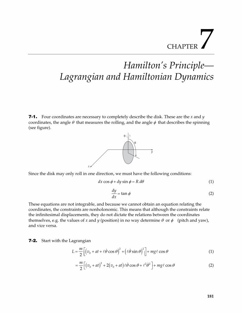
CHAPTER 7 Hamilton’s Principle—
Lagrangian and Hamiltonian Dynamics
7-1. Four coordinates are necessary to completely describe the disk. These are the x and y coordinates, the angle that measures the rolling, and the angle that describes the spinning (see figure).
!
"
x
y
Since the disk may only roll in one direction, we must have the following conditions:
cos sindx dy R d (1)
tandydx
(2)
These equations are not integrable, and because we cannot obtain an equation relating the coordinates, the constraints are nonholonomic. This means that although the constraints relate the infinitesimal displacements, they do not dictate the relations between the coordinates themselves, e.g. the values of x and y (position) in no way determine or (pitch and yaw), and vice versa.
7-2. Start with the Lagrangian
2 2
0 cos sin cos2m
at mgL v (1)
2 2 20 02 cos
2m
v at v at mg cos (2)
181
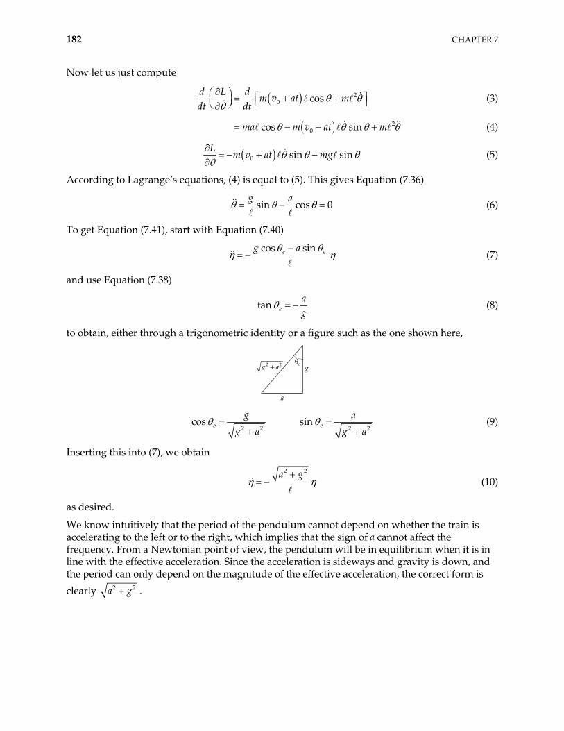
182 CHAPTER 7
Now let us just compute
20 cos
d L dm v at m
dt dt (3)
20cos sinma m v at m (4)
0 sin sinL
m v at mg (5)
According to Lagrange’s equations, (4) is equal to (5). This gives Equation (7.36)
sin cos 0g a
(6)
To get Equation (7.41), start with Equation (7.40)
cos sineg a e (7)
and use Equation (7.38)
tan eag
(8)
to obtain, either through a trigonometric identity or a figure such as the one shown here,
g
a
"eg a2 2+
2 2
sg
g aco e
2 2sin e
a
g a (9)
Inserting this into (7), we obtain
2 2a g
(10)
as desired.
We know intuitively that the period of the pendulum cannot depend on whether the train is accelerating to the left or to the right, which implies that the sign of a cannot affect the frequency. From a Newtonian point of view, the pendulum will be in equilibrium when it is in line with the effective acceleration. Since the acceleration is sideways and gravity is down, and the period can only depend on the magnitude of the effective acceleration, the correct form is
clearly 2 2a g .
HAMILTON’S PRINCIPLE—LAGRANGIAN AND HAMILTONIAN DYNAMICS 183
7-3.
"
#! "
R
If we take angles and as our generalized coordinates, the kinetic energy and the potential energy of the system are
2 21
2 2T m R I
1 (1)
cosU R R mg (2)
where m is the mass of the sphere and where U = 0 at the lowest position of the sphere. I is the moment of inertia of sphere with respect to any diameter. Since 22 5I m , the Lagrangian becomes
2 2 2 21 1cos
2 5U m R m R R mgL T (3)
When the sphere is at its lowest position, the points A and B coincide. The condition A0 = B0 gives the equation of constraint:
,f R 0 (4)
Therefore, we have two Lagrange’s equations with one undetermined multiplier:
0
0
fL d Ldt
fL d Ldt
(5)
After substituting (3) and f R and f into (5), we find
2sin 0R mg m R R (6)
220
5m (7)
From (7) we find :
25
m (8)
or, if we use (4), we have
25
m R (9)
Substituting (9) into (6), we find the equation of motion with respect to :
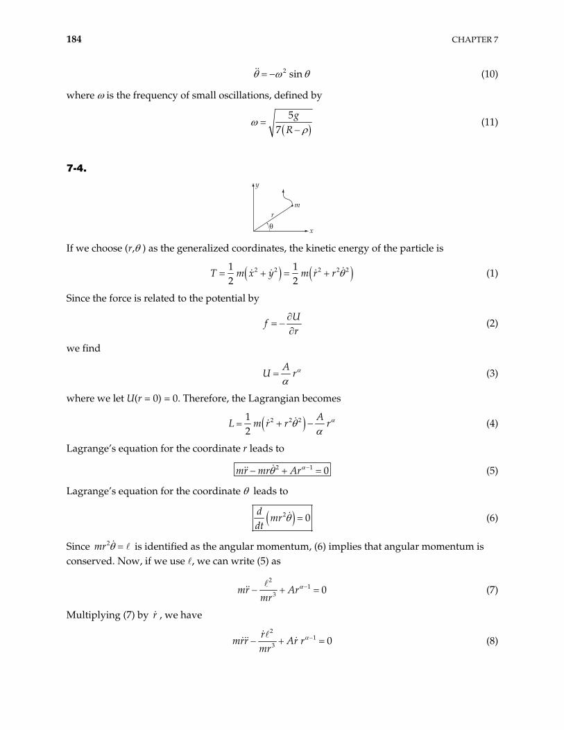
184 CHAPTER 7
2 sin (10)
where is the frequency of small oscillations, defined by
5
7g
R (11)
7-4.
y
m
x
r
"
If we choose (r, ) as the generalized coordinates, the kinetic energy of the particle is
2 2 2 2 21 12 2
T m x y m r r (1)
Since the force is related to the potential by
U
fr
(2)
we find
A
U r (3)
where we let U(r = 0) = 0. Therefore, the Lagrangian becomes
2 2 212
AL m r r r (4)
Lagrange’s equation for the coordinate r leads to
2 1 0mr mr Ar (5)
Lagrange’s equation for the coordinate leads to
2 0d
mrdt
(6)
Since is identified as the angular momentum, (6) implies that angular momentum is conserved. Now, if we use , we can write (5) as
2mr
2
13 0mr Ar
mr (7)
Multiplying (7) by , we have r
2
13 0
rmrr Ar r
mr (8)
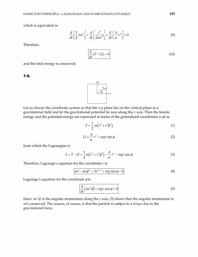
HAMILTON’S PRINCIPLE—LAGRANGIAN AND HAMILTONIAN DYNAMICS 185
which is equivalent to
2
22
10
2 2d d d A
mr rdt dt mr dt
(9)
Therefore,
0d
T Udt
(10)
and the total energy is conserved.
7-5.
! x
y
r m
Let us choose the coordinate system so that the x-y plane lies on the vertical plane in a gravitational field and let the gravitational potential be zero along the x axis. Then the kinetic energy and the potential energy are expressed in terms of the generalized coordinates (r, ) as
2 2 212
T m r r (1)
sinA
U r mgr (2)
from which the Lagrangian is
2 2 21sin
2A
U m r r r mgrL T (3)
Therefore, Lagrange’s equation for the coordinate r is
2 1 sin 0mr mr Ar mg (4)
Lagrange’s equation for the coordinate is
2 cos 0d
mr mgrdt
(5)
Since 2mr is the angular momentum along the z axis, (5) shows that the angular momentum is not conserved. The reason, of course, is that the particle is subject to a torque due to the gravitational force.
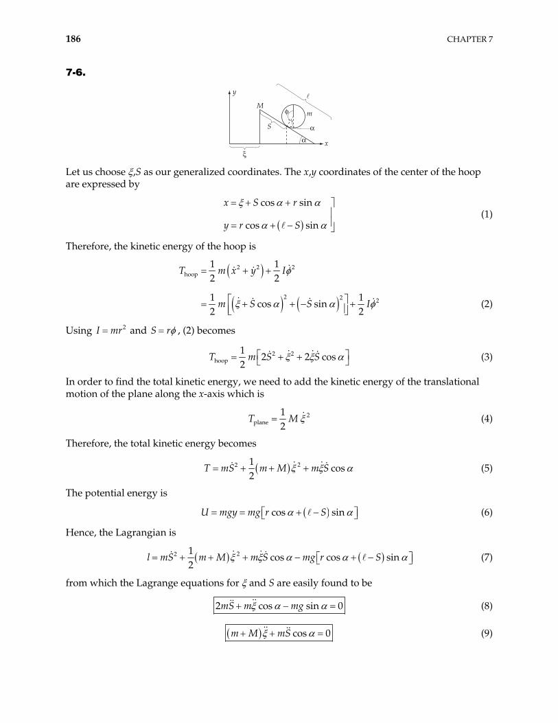
186 CHAPTER 7
7-6.
y
M
S
m
$$
!
%x
Let us choose ,S as our generalized coordinates. The x,y coordinates of the center of the hoop are expressed by
cos sin
cos sin
x S r
y r S (1)
Therefore, the kinetic energy of the hoop is
2 2 2hoop
2 2 2
1 12 2
1 1cos sin
2 2
T m x y I
m S S I (2)
Using and 2I mr S r , (2) becomes
2 2hoop
12 2 cos
2T m S S (3)
In order to find the total kinetic energy, we need to add the kinetic energy of the translational motion of the plane along the x-axis which is
2plane
12
T M (4)
Therefore, the total kinetic energy becomes
22 1cos
2T mS m M m S (5)
The potential energy is
cos sinU mgy mg r S (6)
Hence, the Lagrangian is
22 1cos cos sin
2S m M m S mg r Sl m (7)
from which the Lagrange equations for and S are easily found to be
2 cos sinmS m mg 0 (8)
cos 0m M mS (9)
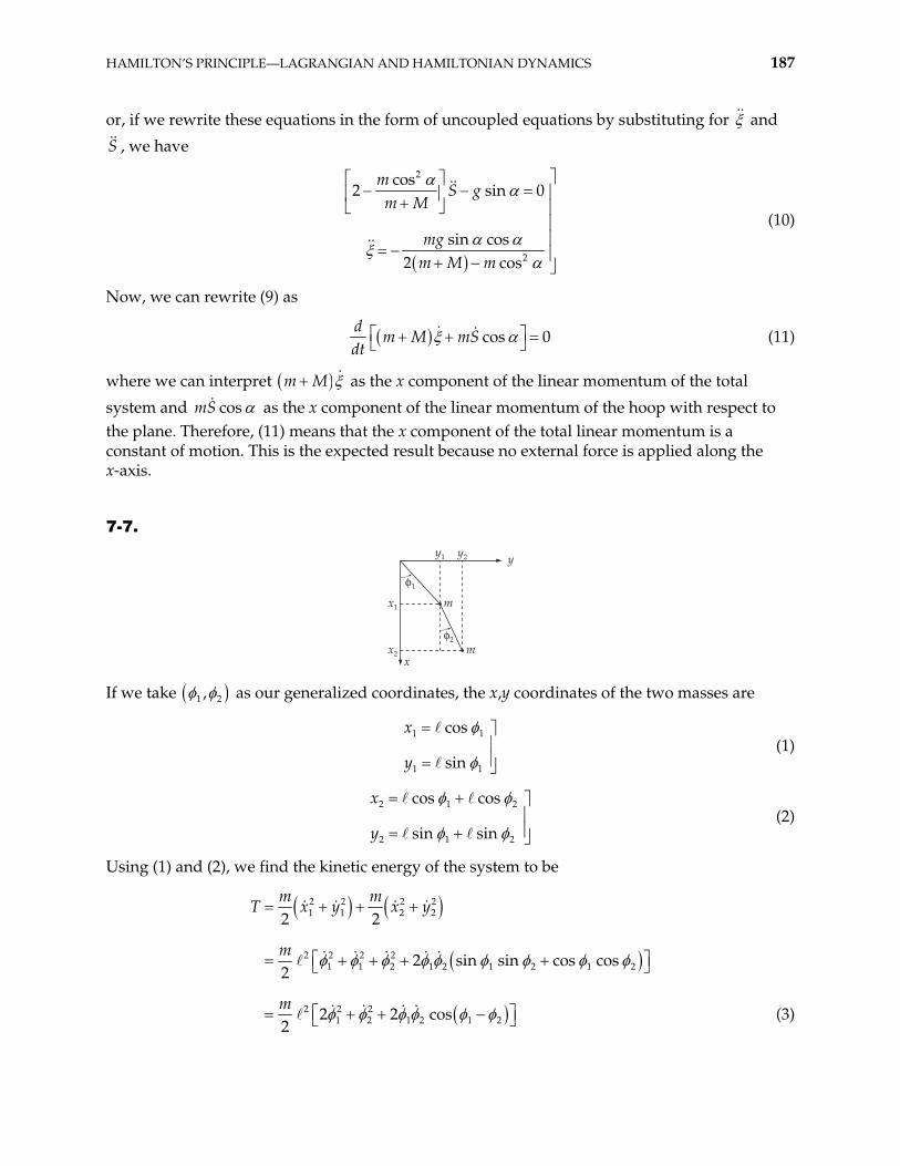
HAMILTON’S PRINCIPLE—LAGRANGIAN AND HAMILTONIAN DYNAMICS 187
or, if we rewrite these equations in the form of uncoupled equations by substituting for and
, we have S
2
2
cos2 si
sin cos2 cos
mS g
m M
mgm M m
n 0
(10)
Now, we can rewrite (9) as
cos 0d
m M mSdt
(11)
where we can interpret m M as the x component of the linear momentum of the total
system and cosmS as the x component of the linear momentum of the hoop with respect to the plane. Therefore, (11) means that the x component of the total linear momentum is a constant of motion. This is the expected result because no external force is applied along the x-axis.
7-7.
x1
y1 y2
x2
m
y
mx
!1
!2
If we take 1 2, as our generalized coordinates, the x,y coordinates of the two masses are
1 1
1 1
cos
sin
x
y (1)
2 1
2 1
cos cos
sin sin
x
y
2
2
(2)
Using (1) and (2), we find the kinetic energy of the system to be
2 2 2 21 1 2 2
2 2 2 21 1 2 1 2 1 2 1 2
2 2 21 2 1 2 1 2
2 2
2 sin sin cos cos2
2 2 cos2
m mT x y x y
m
m (3)
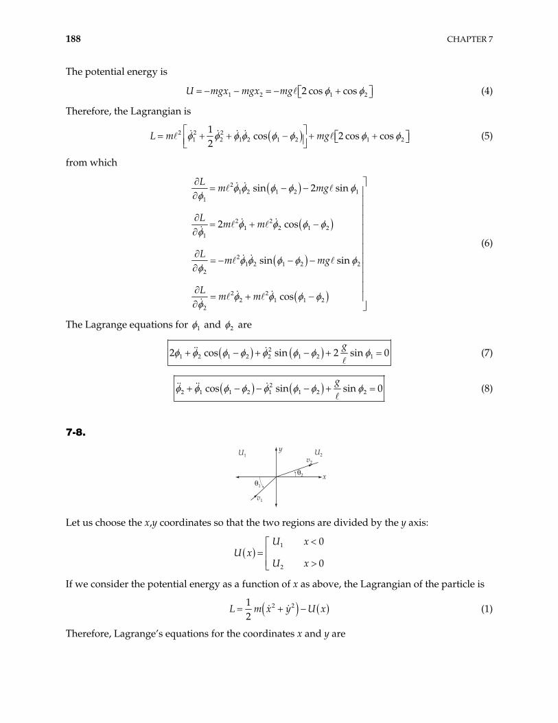
188 CHAPTER 7
The potential energy is
U m 1 2 12 cos cosgx mgx mg 2 (4)
Therefore, the Lagrangian is
2 2 21 2 1 2 1 2 1
1cos 2 cos cos
2mg 2L m (5)
from which
21 2 1 2 1
1
2 21 2 1 2
1
21 2 1 2 2
2
2 22 1 1 2
2
sin 2 sin
2 cos
sin sin
cos
Lm m
Lm m
Lm mg
Lm m
g
(6)
The Lagrange equations for 1 and 2 are
21 2 1 2 2 1 2 1cos sin 2 sin 0
g2 (7)
22 1 1 2 1 1 2 2cos sin sin 0
g (8)
7-8.
v1
v2
"2
"1
U1 U2y
x
Let us choose the x,y coordinates so that the two regions are divided by the y axis:
1
2
0
0
U xU x
U x
If we consider the potential energy as a function of x as above, the Lagrangian of the particle is
2 212
L m x y U x (1)
Therefore, Lagrange’s equations for the coordinates x and y are
HAMILTON’S PRINCIPLE—LAGRANGIAN AND HAMILTONIAN DYNAMICS 189
0dU x
mxdx
(2)
0my (3)
Using the relation
xx x x dpdP dP Pd dxmx mx
dt dt dx dt m dx (4)
(2) becomes
0x x dU xP dPm dx dx
(5)
Integrating (5) from any point in the region 1 to any point in the region 2, we find
2 2
1 1
0x x dU xP dPdx dx
m dx dx (6)
2 1
2 2
2 1 02 2
x xP PU U
m m (7)
or, equivalently,
2 21 1 2
1 12 2
mx U mx U2 (8)
Now, from (3) we have
0d
mydt
and is constant. Therefore, my
1my my2 (9)
From (9) we have
21
1 12 2
my my22 (10)
Adding (8) and (10), we have
21 1 2
1 12 2
mv U mv U22
2
(11)
From (9) we also have
1 1 2sin sinmv mv (12)
Substituting (11) into (12), we find
1 2
1 2 1 2
2 1 1
sin1
sinv U Uv T
(13)
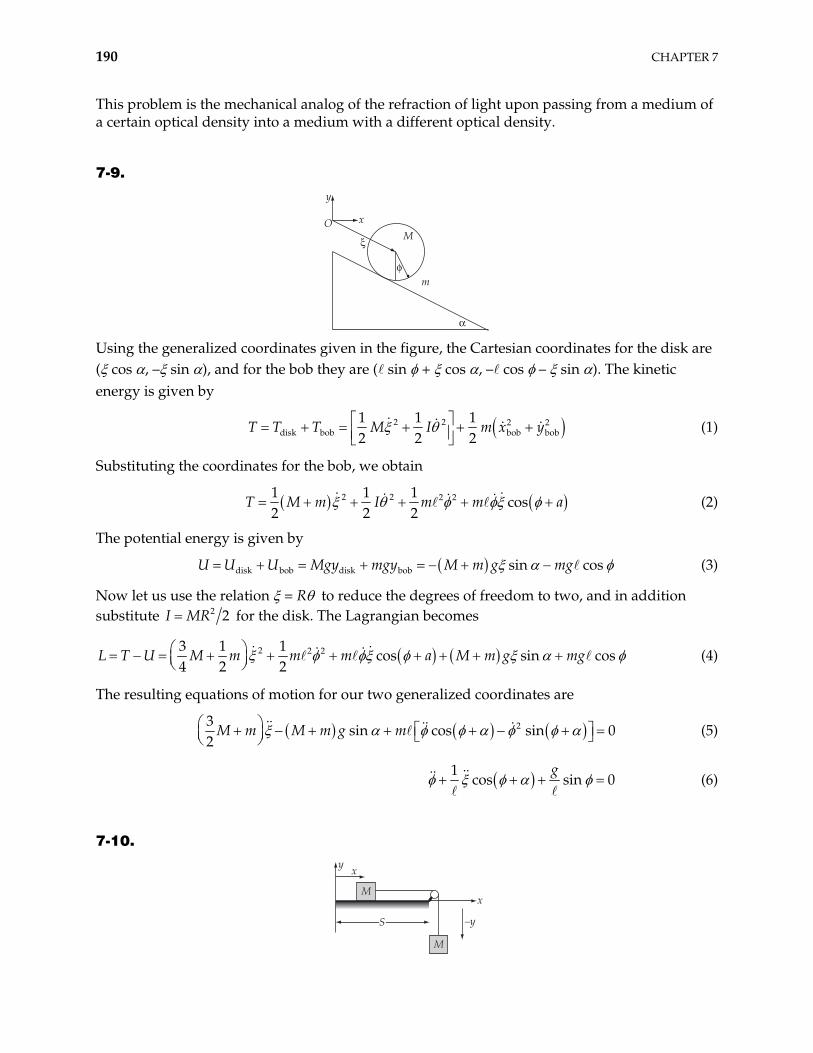
190 CHAPTER 7
This problem is the mechanical analog of the refraction of light upon passing from a medium of a certain optical density into a medium with a different optical density.
7-9.
O x
y
M
m!
$
%
Using the generalized coordinates given in the figure, the Cartesian coordinates for the disk are ( cos , – sin ), and for the bob they are ( sin + cos , – cos – sin ). The kinetic energy is given by
2 2 2 2disk bob bob bob
1 1 12 2 2
T M I m x yT T (1)
Substituting the coordinates for the bob, we obtain
2 2 2 21 1 1cos
2 2 2m I m m aT M (2)
The potential energy is given by
disk bob disk bob sin cosU U Mgy mgy M m g mgU (3)
Now let us use the relation = R to reduce the degrees of freedom to two, and in addition substitute 2 2I MR for the disk. The Lagrangian becomes
2 2 23 1 1cos sin cos
4 2 2L T U M m m m a M m g mg (4)
The resulting equations of motion for our two generalized coordinates are
23sin cos sin 0
2M m M m g m (5)
1
cos sin 0g
(6)
7-10.
MM
MM
y x
x
–yS
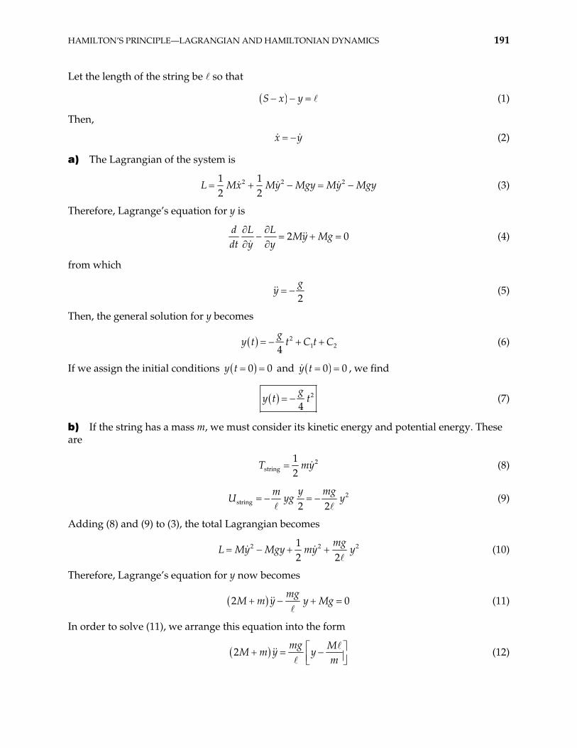
HAMILTON’S PRINCIPLE—LAGRANGIAN AND HAMILTONIAN DYNAMICS 191
Let the length of the string be so that
S x y (1)
Then,
x y (2)
a) The Lagrangian of the system is
2 2 21 12 2
Mx My Mgy My MgyL (3)
Therefore, Lagrange’s equation for y is
2d L L
My Mgdt y y
0 (4)
from which
2g
y (5)
Then, the general solution for y becomes
214
gy t t C t C2 (6)
If we assign the initial conditions 0y t 0 and 0y t 0 , we find
2
4g
y t t (7)
b) If the string has a mass m, we must consider its kinetic energy and potential energy. These are
2string
12
T my (8)
2string 2 2
y mgmU yg y (9)
Adding (8) and (9) to (3), the total Lagrangian becomes
2 212 2
mgL My Mgy my y2 (10)
Therefore, Lagrange’s equation for y now becomes
2mg
M m y y Mg 0 (11)
In order to solve (11), we arrange this equation into the form
2mg M
M m y ym
(12)
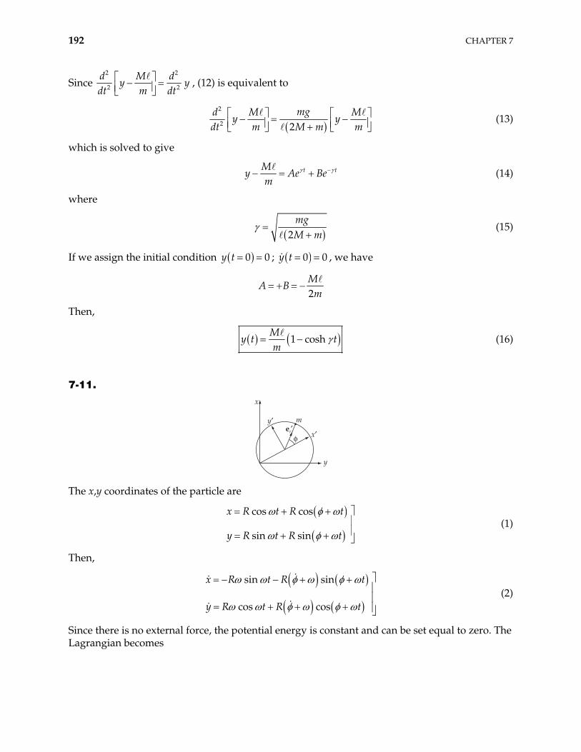
192 CHAPTER 7
Since 2 2
2
d M dy
dt m dt2 y , (12) is equivalent to
2
2 2mgd M M
ydt m M m m
y (13)
which is solved to give
tMy Ae B
mte (14)
where
2
mgM m
(15)
If we assign the initial condition 0 0y t ; 0y t 0 , we have
2M
A Bm
Then,
1 coshM
y t tm
(16)
7-11.
x
x&
m
y
y&
!er&
The x,y coordinates of the particle are
cos cos
sin sin
x R t R t
y R t R t (1)
Then,
sin sin
cos cos
x R t R t
y R t R t (2)
Since there is no external force, the potential energy is constant and can be set equal to zero. The Lagrangian becomes
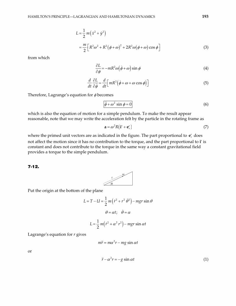
HAMILTON’S PRINCIPLE—LAGRANGIAN AND HAMILTONIAN DYNAMICS 193
2 2
22 2 2 2
12
2 c2
L m x y
mR R R os (3)
from which
2 sinL
mR (4)
2 cosd L d
mRdt dt
(5)
Therefore, Lagrange’s equation for becomes
2 sin 0 (6)
which is also the equation of motion for a simple pendulum. To make the result appear reasonable, note that we may write the acceleration felt by the particle in the rotating frame as
2rRa i e (7)
where the primed unit vectors are as indicated in the figure. The part proportional to re does not affect the motion since it has no contribution to the torque, and the part proportional to i is constant and does not contribute to the torque in the same way a constant gravitational field provides a torque to the simple pendulum.
7-12.
rm
" Put the origin at the bottom of the plane
2 2 21sin
2U m r r mgrL T
;t
22 21sin
2L m r r mgr t
Lagrange’s equation for r gives
2 sinmr m r mg t
or
2 sinr r g t (1)
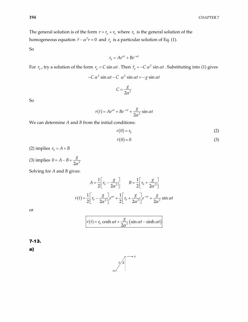
194 CHAPTER 7
The general solution is of the form p hrr r where is the general solution of the
homogeneous equation and hr
2 0r r pr is a particular solution of Eq. (1).
So
t thr Ae Be
For pr , try a solution of the form r C sinp t . Then 2 sinpr C t . Substituting into (1) gives
2 2sin sin sinC t C t g t
22g
C
So
2 sin2
t t gr t Ae Be t
We can determine A and B from the initial conditions:
00r r (2)
0 0r (3)
(2) implies 0r A B
(3) implies 22g
A B0
Solving for A and B gives:
0 02 2
1 12 2 2 2
g gA r B r
0 02 2
1 1sin
2 2 2 2 2t tg g g
r e r e t2r t
or
0 2cosh sin sinh2
gr t t tr t
7-13.
a)
"
a
b
m
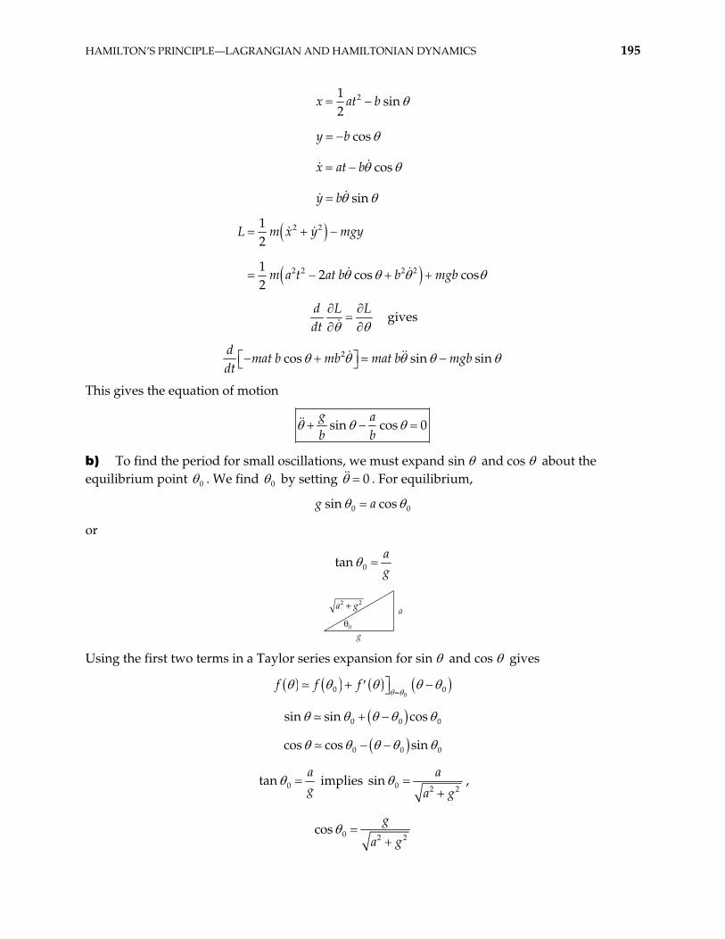
HAMILTON’S PRINCIPLE—LAGRANGIAN AND HAMILTONIAN DYNAMICS 195
21sin
2
cos
cos
sin
x at b
y b
x at b
y b
2 2
2 2 2 2
12
12 cos cos
2
L m x y mgy
m a t at b b mgb
d L Ldt
gives
2cos sin sinmat b mb mat b mgbdtd
This gives the equation of motion
sin cos 0g ab b
b) To find the period for small oscillations, we must expand sin and cos about the equilibrium point 0 . We find 0 by setting 0 . For equilibrium,
0 0sin cosg a
or
0tanag
g
a"0
a g2 2+
Using the first two terms in a Taylor series expansion for sin and cos gives
0
0 0f f f
0 0sin sin cos 0
0 0cos cos sin 0
0tanag
implies 0 2 2sin
a
a g,
0 2 2cos
g
a g
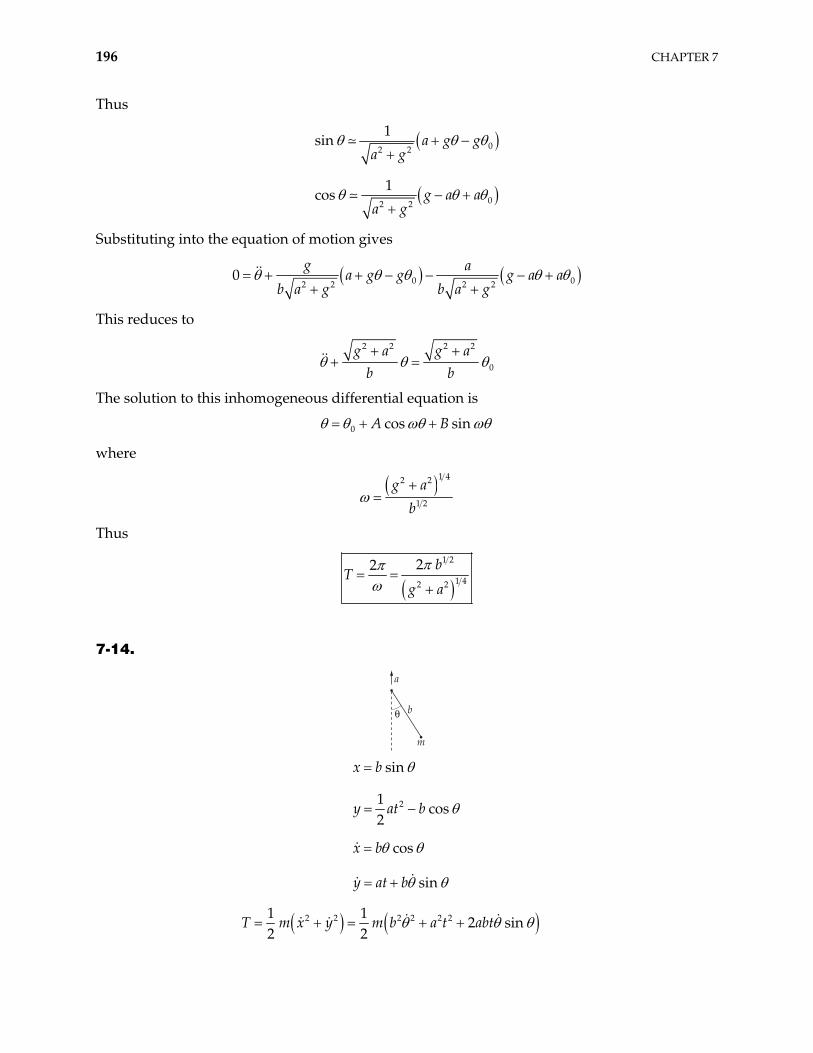
196 CHAPTER 7
Thus
02 2
1sin a g g
a g
02 2
1cos g a a
a g
Substituting into the equation of motion gives
0 02 2 2 2
g aa g g g a a
b a g b a g0
This reduces to
2 2 2 2
0
g a g ab b
The solution to this inhomogeneous differential equation is
0 cos sinA B
where
1 42 2
1 2
g a
b
Thus
1 2
1 42 2
22 bT
g a
7-14.
"
a
b
m
2
sin
1cos
2
cos
sin
x b
y at b
x b
y at b
2 2 2 2 2 21 12 sin
2 2x y m b a t abtT m
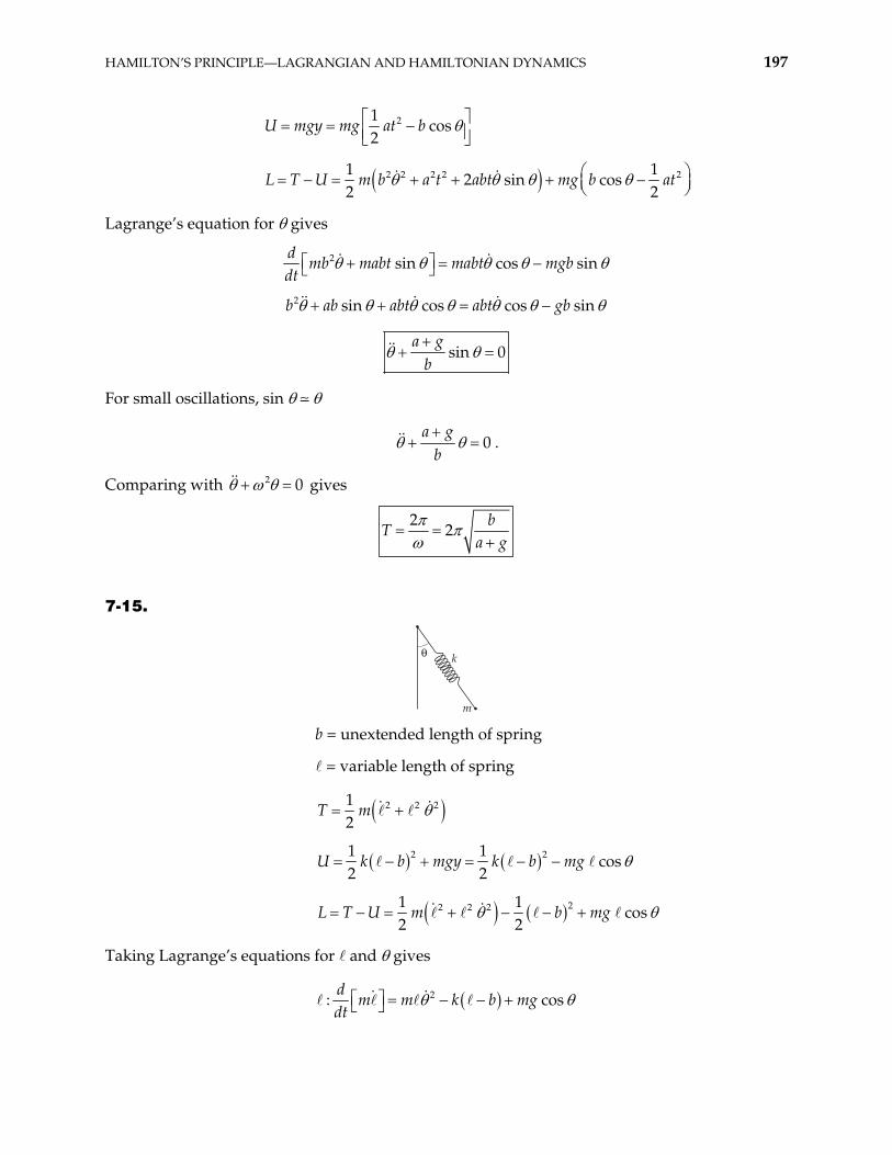
HAMILTON’S PRINCIPLE—LAGRANGIAN AND HAMILTONIAN DYNAMICS 197
21cos
2gy mg at bU m
2 2 2 2 21 12 sin cos
2 2U m b a t abt mg b atL T
Lagrange’s equation for gives
2 sin cos sind
mb mabt mabt mgbdt
b a2 sin cos cos sinb abt abt gb
sin 0a g
b
For small oscillations, sin
0a g
b.
Comparing with gives 2 0
2
2b
Ta g
7-15.
k
m
"
b = unextended length of spring
= variable length of spring
2 2 212
T m
2 21 1cos
2 2b mgy k b mgU k
22 2 21 1cos
2 2U m b mgL T
Taking Lagrange’s equations for and gives
2: cd
m m k b mgdt
os
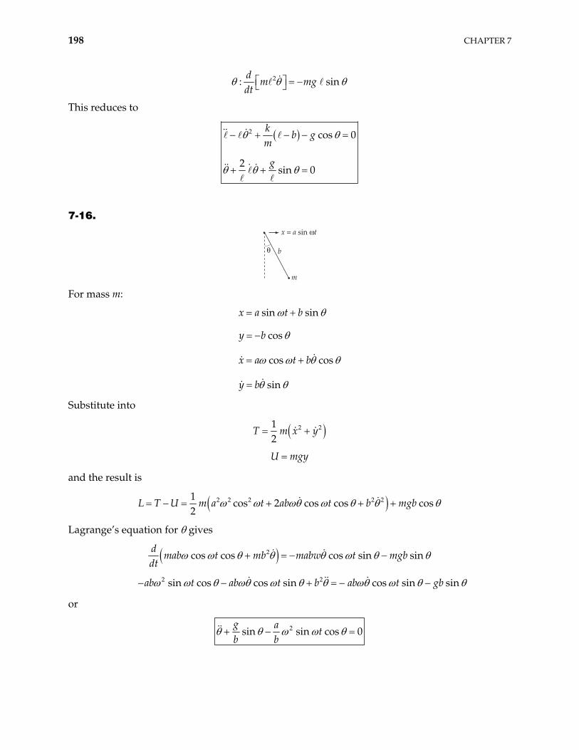
198 CHAPTER 7
2: sd
m mgdt
in
This reduces to
2 cos 0
2sin 0
kb g
m
g
7-16.
"
m
b
x = a sin 't
For mass m:
sin sin
cos
cos cos
sin
x a t b
y b
x a t b
y b
Substitute into
2 212
T m x y
U mgy
and the result is
2 2 2 2 21cos 2 cos cos cos
2L T U m a t ab t b mgb
Lagrange’s equation for gives
cod 2s cos cos sin sinmab t mb mabw t mgbdt
2 2sin cos cos sin cos sin sinab t ab t b ab t gb
or
2sin sin cos 0g a
tb b
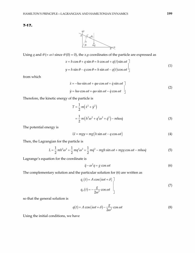
HAMILTON’S PRINCIPLE—LAGRANGIAN AND HAMILTONIAN DYNAMICS 199
7-17.
"
"
A
B
C
y
hmg
q
Using q and (= t since (0) = 0), the x,y coordinates of the particle are expressed as
cos sin cos sin
sin cos sin cos
x h q h t q t t
y h q h t q t t (1)
from which
sin cos sin
cos sin cos
x h t q t q t
y h t q t q t (2)
Therefore, the kinetic energy of the particle is
2 2
2 2 2 2 2
12
12
T m x y
m h q q mh q (3)
The potential energy is
sin cosU mgy mg h t q t (4)
Then, the Lagrangian for the particle is
2 2 2 2 21 1 1sin cos
2 2 2mh mq mq mgh t mgq t mh qL
t
(5)
Lagrange’s equation for the coordinate is
2 cosq q g (6)
The complementary solution and the particular solution for (6) are written as
2
cos
cos2
c
P
q t A i t
gq t t
(7)
so that the general solution is
2cos cos2
gq t A i t t (8)
Using the initial conditions, we have
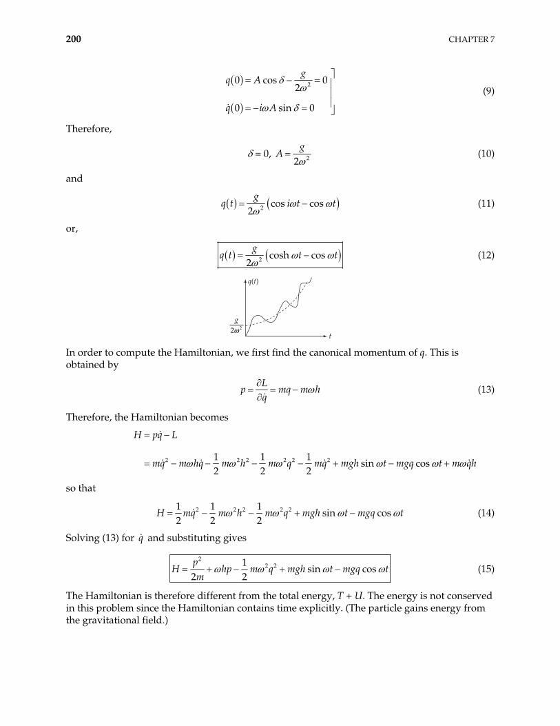
200 CHAPTER 7
20 cos 0
2
0 sin 0
gq A
q i A
(9)
Therefore,
= 0, 22g
A (10)
and
2 cos cos2
gq t i t t (11)
or,
2 cosh cos2
gq t t t (12)
q(t)
t
g2 2'
In order to compute the Hamiltonian, we first find the canonical momentum of q. This is obtained by
L
p mq m hq
(13)
Therefore, the Hamiltonian becomes
2 2 2 2 2 21 1 1
sin cos2 2 2
H pq L
mq m hq m h m q mq mgh t mgq t m qh
so that
2 2 2 2 21 1 1sin cos
2 2 2H mq m h m q mgh t mgq t (14)
Solving (13) for and substituting gives q
2
2 21sin cos
2 2p
H hp m q mgh t mgq tm
(15)
The Hamiltonian is therefore different from the total energy, T + U. The energy is not conserved in this problem since the Hamiltonian contains time explicitly. (The particle gains energy from the gravitational field.)
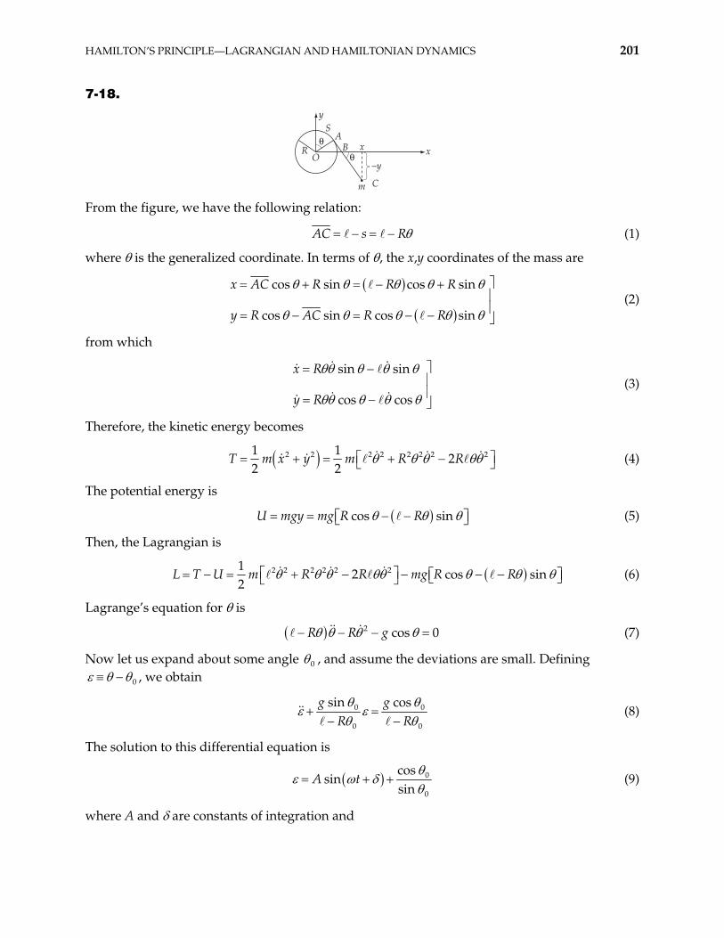
HAMILTON’S PRINCIPLE—LAGRANGIAN AND HAMILTONIAN DYNAMICS 201
7-18.
""
yS
RO
AB
Cm
x
–yx
From the figure, we have the following relation:
AC s R (1)
where is the generalized coordinate. In terms of , the x,y coordinates of the mass are
cos sin cos sin
cos sin cos sin
x AC R R R
y R AC R R (2)
from which
sin sin
cos cos
x R
y R (3)
Therefore, the kinetic energy becomes
2 2 2 2 2 2 2 21 12
2 2x y m R RT m (4)
The potential energy is
cos singy mg R RU m (5)
Then, the Lagrangian is
2 2 2 2 2 212 cos
2L T U m R R mg R R sin (6)
Lagrange’s equation for is
2 cos 0R R g (7)
Now let us expand about some angle 0 , and assume the deviations are small. Defining
0 , we obtain
0
0 0
sin cosg gR R
0 (8)
The solution to this differential equation is
0
0
cossin
sinA t (9)
where A and are constants of integration and
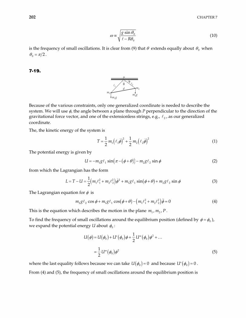
202 CHAPTER 7
0
0
singR
(10)
is the frequency of small oscillations. It is clear from (9) that extends equally about 0 when
0 2 .
7-19.
PP
m1
m2
m2gm1g
d"
!
Because of the various constraints, only one generalized coordinate is needed to describe the system. We will use , the angle between a plane through P perpendicular to the direction of the gravitational force vector, and one of the extensionless strings, e.g., , as our generalized coordinate.
2
The, the kinetic energy of the system is
2
1 1 2 21 12 2
T m m2
(1)
The potential energy is given by
1 1 2 2sin sing m gU m (2)
from which the Lagrangian has the form
2 2 21 1 2 2 1 1 2 2
1sin sin
2U m m m g m gL T (3)
The Lagrangian equation for is
2 22 2 1 1 1 1 2 2cos cos 0m g m mm g (4)
This is the equation which describes the motion in the plane . 1 2, ,m m P
To find the frequency of small oscillations around the equilibrium position (defined by 0 ), we expand the potential energy U about 0 :
20 0 0
20
12
12
U U U U
U (5)
where the last equality follows because we can take 0 0U and because 0 0U .
From (4) and (5), the frequency of small oscillations around the equilibrium position is
HAMILTON’S PRINCIPLE—LAGRANGIAN AND HAMILTONIAN DYNAMICS 203
022
1 1 2 2
Um m 2 (6)
The condition 0 0U gives
2 2 1 10
1 1
costan
sinm m
m (7)
or,
2 2 1 10 1 22 2 2 2
1 1 2 2 1 2 1 2
cosn
2 cos
m m
m m m msi (8)
Then from (2), (7), and (8), 0U is found to be
0 0 2 2 1 1 1 1 0
2 2 22 2 1 1 1 1
2 2 1 11 22 2 2 22 2 1 11 1 2 2 2 1 2 1
1 22 2 2 21 1 2 2 2 1 2 1
sin cos sin cot
cos sincos
cos2 cos
2 cos
U g m m m
g m m mm m
m mm m m m
g m m m m (9)
Finally, from (6) and (9), we have
1 22 2 2 2
1 1 2 2 1 2 1 222 2
1 1 2 2
2 cosm m m mg
m m (10)
which, using the relation,
2 21 2
1 2
cos2
d2
(11)
can be written as
1 22 2 21 2 1 1 2 2 1 2
2 21 1 2 2
g m m m m d m m
m m2 (12)
Notice that 2 degenerates to the value g appropriate for a simple pendulum when d 0 (so that ). 1 2
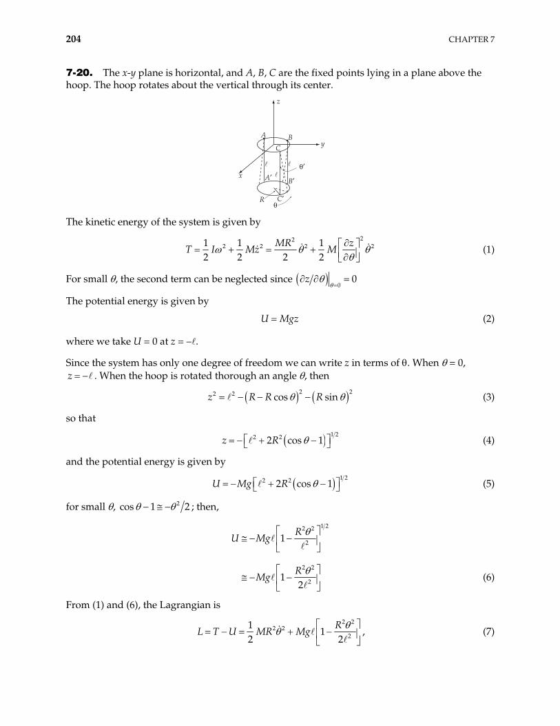
204 CHAPTER 7
7-20. The x-y plane is horizontal, and A, B, C are the fixed points lying in a plane above the hoop. The hoop rotates about the vertical through its center.
z
A B
B&
y
x
R
C
C&
A&"&
" The kinetic energy of the system is given by
22
2 2 21 1 12 2 2 2
MR zMz M 2T I (1)
For small , the second term can be neglected since 0
0z
The potential energy is given by
U Mgz (2)
where we take U = 0 at z = – .
Since the system has only one degree of freedom we can write z in terms of . When = 0, z . When the hoop is rotated thorough an angle , then
22 2 cos sinz R R R
2 (3)
so that
1 22 22 cos 1z R (4)
and the potential energy is given by
1 22 22 cos 1U Mg R (5)
for small , 2s 1 2co ; then,
1 22 2
2
2 2
2
1
12
RU Mg
RMg (6)
From (1) and (6), the Lagrangian is
2 2
2 22
11
2 2R
U MR MgL T , (7)
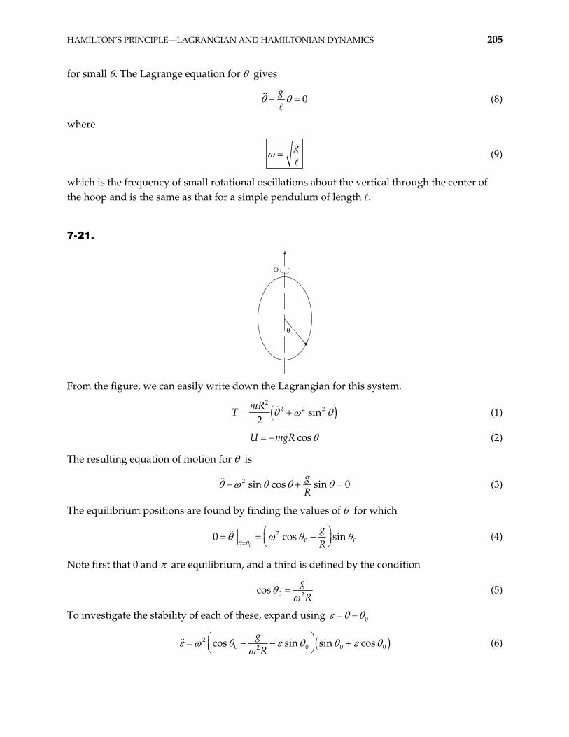
HAMILTON’S PRINCIPLE—LAGRANGIAN AND HAMILTONIAN DYNAMICS 205
for small . The Lagrange equation for gives
0g
(8)
where
g
(9)
which is the frequency of small rotational oscillations about the vertical through the center of the hoop and is the same as that for a simple pendulum of length .
7-21.
'
"
From the figure, we can easily write down the Lagrangian for this system.
2
2 2 2sin2
mRT (1)
cosU mgR (2)
The resulting equation of motion for is
2 sin cos sin 0gR
(3)
The equilibrium positions are found by finding the values of for which
0
200 cos
gR 0sin (4)
Note first that 0 and are equilibrium, and a third is defined by the condition
0 2cosgR
(5)
To investigate the stability of each of these, expand using 0
20 0 02cos sin sin cos
gR 0 (6)
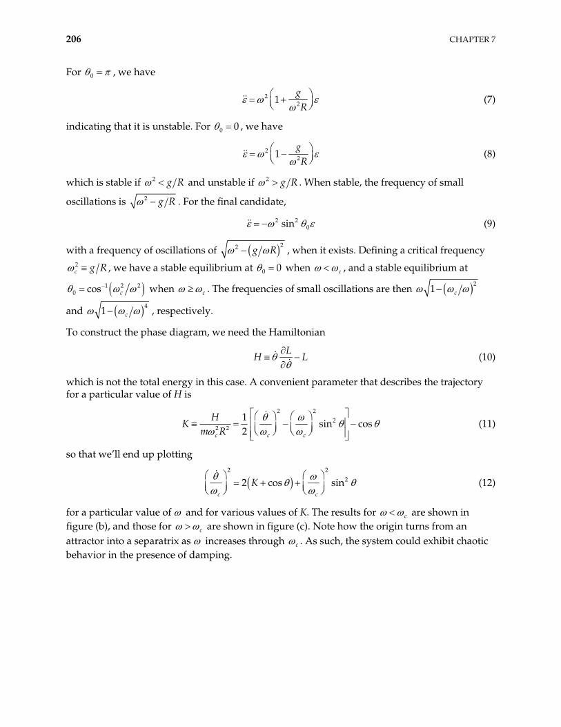
206 CHAPTER 7
For 0 , we have
221gR
(7)
indicating that it is unstable. For 0 0 , we have
221gR
(8)
which is stable if 2 g R and unstable if 2 g R . When stable, the frequency of small
oscillations is 2 g R . For the final candidate,
2 20sin (9)
with a frequency of oscillations of 22 g R , when it exists. Defining a critical frequency
2c g R , we have a stable equilibrium at 0 0 when c , and a stable equilibrium at
1 2 20 cos c when c . The frequencies of small oscillations are then
21 c
and 4
1 c , respectively.
To construct the phase diagram, we need the Hamiltonian
L
H L (10)
which is not the total energy in this case. A convenient parameter that describes the trajectory for a particular value of H is
2 2
22 2
1sin cos
2c c c
Hm R
K (11)
so that we’ll end up plotting
2 2
22 cos sinc c
K (12)
for a particular value of and for various values of K. The results for c are shown in figure (b), and those for c are shown in figure (c). Note how the origin turns from an attractor into a separatrix as increases through c . As such, the system could exhibit chaotic behavior in the presence of damping.
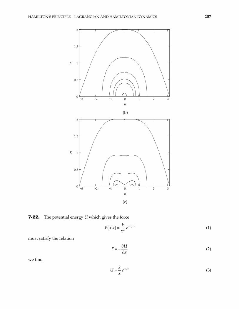
HAMILTON’S PRINCIPLE—LAGRANGIAN AND HAMILTONIAN DYNAMICS 207
3 2 1 0 1 20
0.5
1
1.5
2
3
K
!
(b)
3 2 1 0 1 20
0.5
1
1.5
2
3
K
!
(c)
7-22. The potential energy U which gives the force
2, tkF x t e
x (1)
must satisfy the relation
U
Fx
(2)
we find
tkU e
x (3)
208 CHAPTER 7
Therefore, the Lagrangian is
212
tkL T U mx e
x (4)
The Hamiltonian is given by
xL
H p x L x Lx
(5)
so that
2
2txp k
Hm x
e (6)
The Hamiltonian is equal to the total energy, T + U, because the potential does not depend on velocity, but the total energy of the system is not conserved because H contains the time explicitly.
7-23. The Hamiltonian function can be written as [see Eq. (7.153)]
j jj
H p q L (1)
For a particle which moves freely in a conservative field with potential U, the Lagrangian in rectangular coordinates is
2 2 212
L m x y z U
and the linear momentum components in rectangular coordinates are
x
y
z
Lp mx
x
p my
p mz
(2)
2 2 2 2 2 2
2 2 2 2 2 2
12
1 12 2 x y z
H mx my mz m x y z U
m x y z U p p pm
(3)
which is just the total energy of the particle. The canonical equations are [from Eqs. (7.160) and (7.161)]
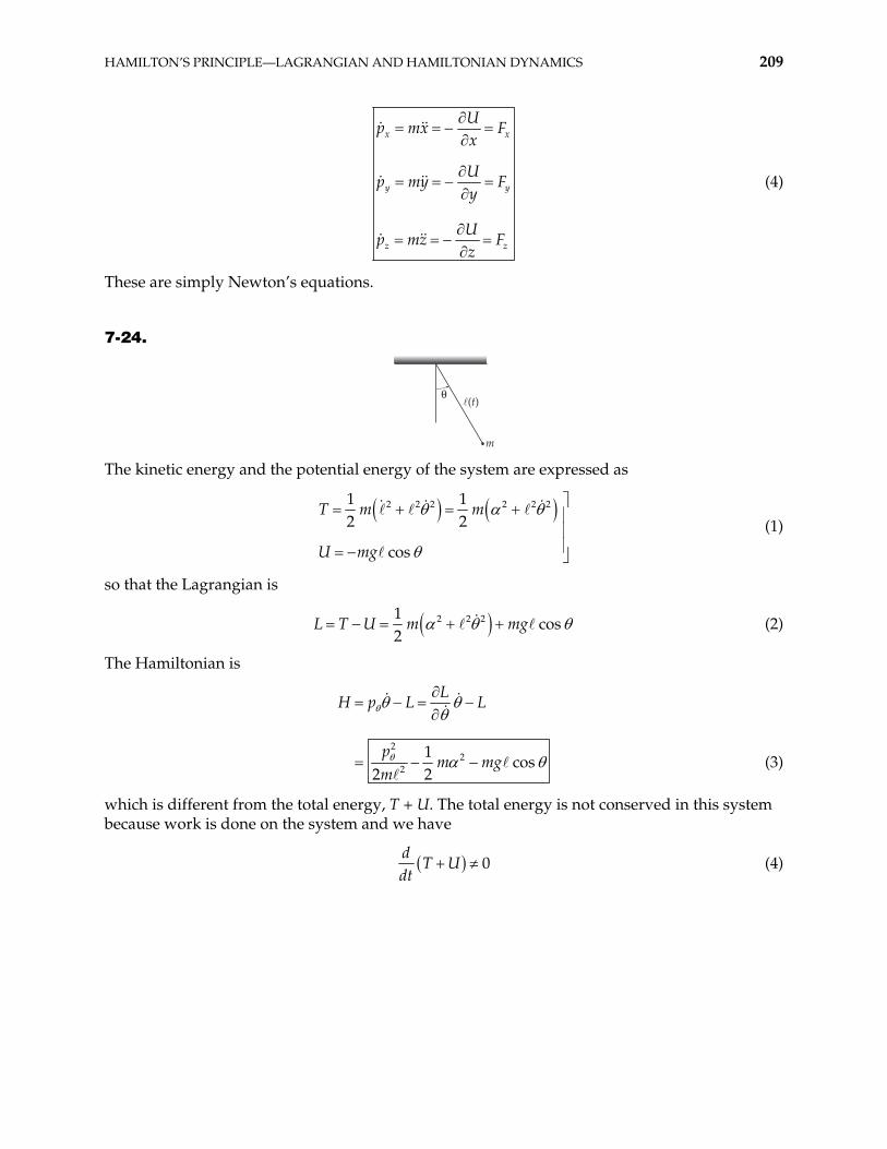
HAMILTON’S PRINCIPLE—LAGRANGIAN AND HAMILTONIAN DYNAMICS 209
x x
y y
z z
Up mx F
x
Up my F
y
Up mz F
z
(4)
These are simply Newton’s equations.
7-24.
"
m The kinetic energy and the potential energy of the system are expressed as
2 2 2 2 2 21 1
2 2
cos
T m m
U mg
(1)
so that the Lagrangian is
2 2 21cos
2U m mgL T (2)
The Hamiltonian is
2
22
1cos
2 2
LH p L L
pm mg
m (3)
which is different from the total energy, T + U. The total energy is not conserved in this system because work is done on the system and we have
0d
T Udt
(4)
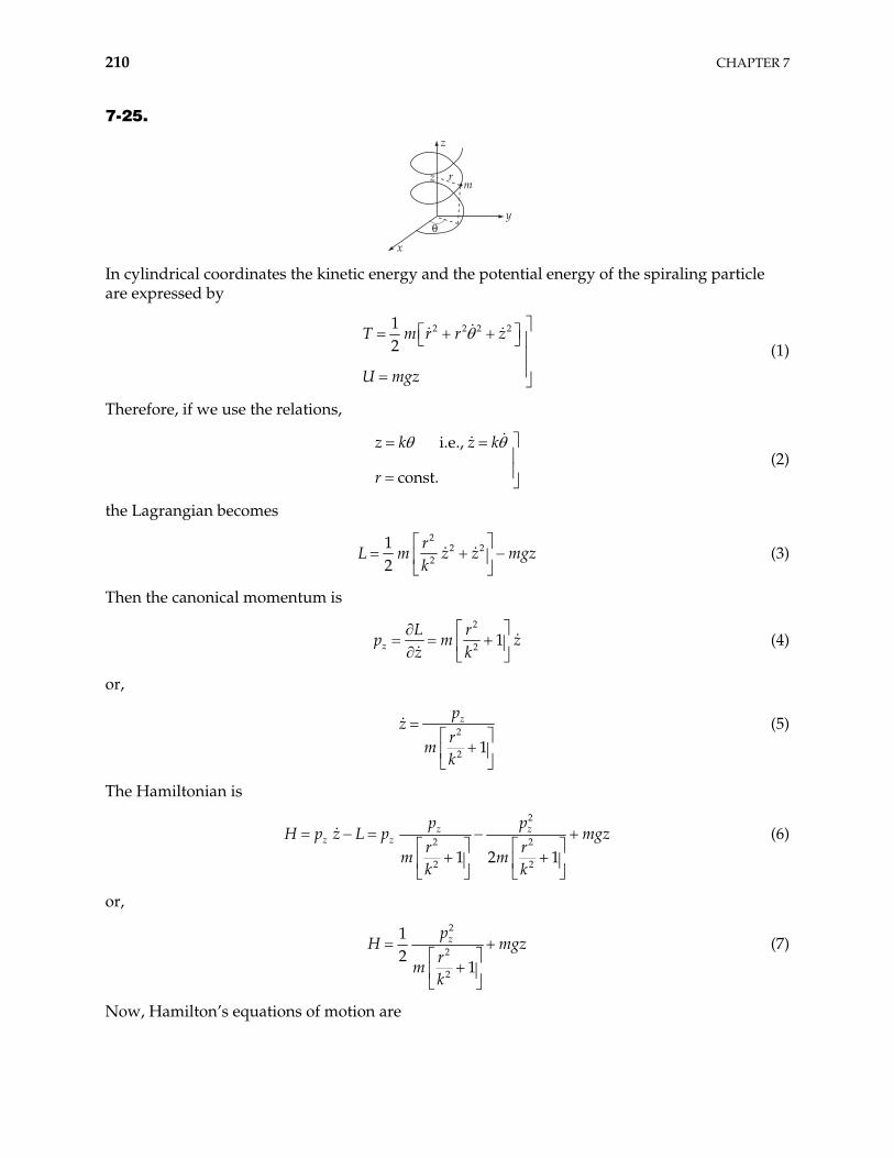
210 CHAPTER 7
7-25.
z
mz r
y
x
"
In cylindrical coordinates the kinetic energy and the potential energy of the spiraling particle are expressed by
2 2 2 21
2T m r r z
U mgz
(1)
Therefore, if we use the relations,
i.e.,
const.
z k z k
r (2)
the Lagrangian becomes
2
2 22
12
rL m z z mg
kz (3)
Then the canonical momentum is
2
2 1zL r
p mz k
z (4)
or,
2
2 1
zpz
rm
k
(5)
The Hamiltonian is
2
2 2
2 21 2 1
z zz z
p pH p z L p mgz
r rm m
k k
(6)
or,
2
2
2
12
1
zpH mgz
rm
k
(7)
Now, Hamilton’s equations of motion are
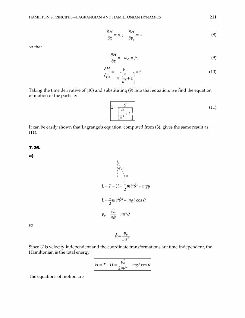
HAMILTON’S PRINCIPLE—LAGRANGIAN AND HAMILTONIAN DYNAMICS 211
zH
pz
; z
Hz
p (8)
so that
zH
mg pz
(9)
2
2 1
z
z
pHz
p rm
k
(10)
Taking the time derivative of (10) and substituting (9) into that equation, we find the equation of motion of the particle:
2
2 1
gz
rk
(11)
It can be easily shown that Lagrange’s equation, computed from (3), gives the same result as (11).
7-26.
a)
"
m
2 212
L T U m mgy
2 21cos
2L m mg
2Lp m
so
2
pm
Since U is velocity-independent and the coordinate transformations are time-independent, the Hamiltonian is the total energy
2
2 cos2
pH T U mg
m
The equations of motion are
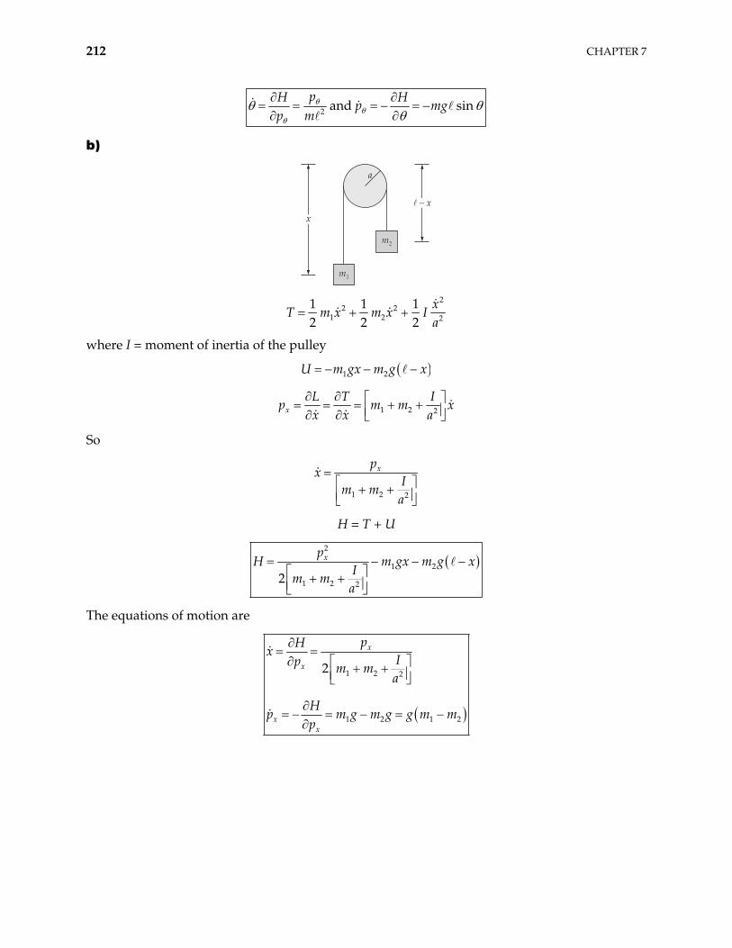
212 CHAPTER 7
2 and sinpH H
p mgp m
b)
a
m2m2
m1m1
x
2
2 21 2 2
1 1 12 2 2
xT m x m x I
a
where I = moment of inertia of the pulley
1 2U m gx m g x
1 2 2xL T I
p m m xx x a
So
1 2 2
xpx
Im m
a
H = T + U
2
1 2
1 2 22
xpH m gx m g x
Im ma
The equations of motion are
1 2 2
1 2 1 2
2
x
x
xx
pHx
Ip m ma
Hp m g m g g m m
p
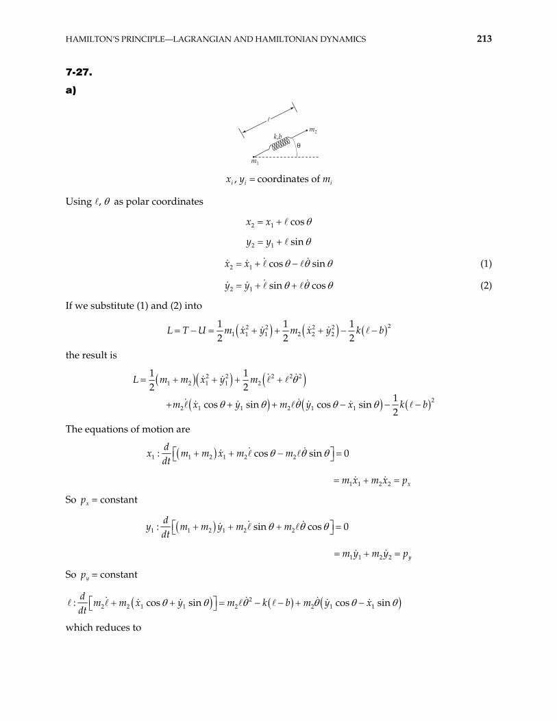
HAMILTON’S PRINCIPLE—LAGRANGIAN AND HAMILTONIAN DYNAMICS 213
7-27.
a)
m2
m1
k,b"
, coordinates ofi ix y m i
Using , as polar coordinates
2 1 cosx x
2 1 siny y
2 1 cos sinx x (1)
2 1 sin cosy y (2)
If we substitute (1) and (2) into
22 2 2 21 1 1 2 2 2
1 1 12 2 2
U m x y m x y k bL T
the result is
2 2 2 2 21 2 1 1 2
22 1 1 2 1 1
1 12 2
1cos sin cos sin
2
L m m x y m
m x y m y x k b
The equations of motion are
1 1 2 1 2 2
1 1 2 2
: cos sin 0
x
dx m m x m m
dt
m x m x p
So = constant xp
1 1 2 1 2 2
1 1 2 2
: sin cos 0
y
dy m m y m m
m y m y p
dt
So yp = constant
22 2 1 1 2 2 1 1: cos sin cos sin
dm m x y m k b m y x
dt
which reduces to
214 CHAPTER 7
21 1
2
cos sin 0k
x y bm
22 2 1 1
2 1 1 2 1 1
: cos sin
sin cos cos sin
dm m y x
dtm x y m x y
which reduces to
1 1cos sin2
0y x
b) As was shown in (a)
1
constantxL
px
1
constantyL
py
(total linear momentum)
c) Using L from part (a)
1 1 2 1 2 2
1
cos sinxL
p m m x m mx
1 1 2 1 2 2
1
sin cosyL
p m m y m my
2 1 2 1 2cos sinL
p m x m y m
22 1 2 1 2sin cosp m x m y m
Inverting these equations gives (after much algebra)
11
1
sin1cosxx p p
mp
11
1
cos1sinyy p p
mp
1 1
1 2
1 2
1cos sinx y
m mp p p
m m
1 1
1 2
1 2
1sin cosx y
m mp p p
m m
Since the coordinate transformations are time independent, and U is velocity independent,
H T U
Substituting using the above equations for in terms of gives iq ip
HAMILTON’S PRINCIPLE—LAGRANGIAN AND HAMILTONIAN DYNAMICS 215
1 1 1 1
1 1
22 2 21 2
21 2
2
12 cos sin
21
2 sin cos2
x y x y
x y
pm mH p p p p p p
m mp
p p k b
The equations of motion are
1
1
11
sin1cosx
x
Hx p p
p mp
1
1
11
cos1siny
y
Hy p p
p mp
1 1
1 2
1 2
1cos sinx y
m mHp p p
p m m
1 1
1 2
1 2
1sin cosx y
m mHp p p
p m m
1 1
1 1
0 0x yH H
p px y
1 1
21 2
3 21 2 1
sin cosx y
m m p pHp p p k
m m mb
1 1 1 1
1 1
sin cos cos sinx y x yp pH
p p p p pm m
Note: This solution chooses as its generalized coordinates what the student would most likely choose at this point in the text. If one looks ahead to Section 8.2 and 8.3, however, it would show another choice of generalized coordinates that lead to three cyclic coordinates ( , , and ), as shown in those sections.
CMx CMy
7-28. so 2F kr 1U kr
2 2 212
kL T U m r r
r
so rr
pLp mr r
r m
22so
pLp mr
mr
Since the coordinate transformations are independent of t, and the potential energy is velocity-independent, the Hamiltonian is the total energy.
216 CHAPTER 7
2 2 2
2 22
2 2 4
2 2
2
12
12
2 2
r
r
kH T U m r r
r
p p km r
m m r r
p p kH
m mr r
Hamilton’s equations of motion are
2
2
3 2
0
r
r
r
p pH Hr
p m p
pH kp
r mr r
Hp
mr
7-29.
a
k
m"
b = unextended length of spring
= variable length of spring
a) sin sin cosx x
21cos cos sin
2y at y at
Substituting into 2 2
2
12
12
T m x y
U mgy k b
gives 2
22 2 2 2 212 sin cos cos
2 2at k
L T U m a t at mg b2
Lagrange’s equations give:
HAMILTON’S PRINCIPLE—LAGRANGIAN AND HAMILTONIAN DYNAMICS 217
2: cos sin cosd
m amt m mat mg k bdt
2: sin sin sin cosd
m mat mat mg matdt
Upon simplifying, the equations of motion reduce to:
2 cos 0
2sin 0
ka g b
m
a g
b) cos or cospL
p m mat atm
(1)
2 sinL
p m mat
or 2
sinp atm
(2)
Since the transformation equations relating the generalized coordinates to rectangular coordinates are not time-independent, the Hamiltonian is not the total energy.
i iH p q L p p L
Substituting (1) and (2) for and and simplifying gives
2 2
2 22
1 1sin cos cos
2 2 2 2p p at
H p atp k b mgat mm m
g
The equations for and are
2 sin
cos agreeing with (1) and (2)
pH atp m
pHat
p m
The equations for and p p are
2
2 3sin cospH at
k b mgm
p p
or
2
2 3sin cos 0pat
k b mgm
p p
cos sin sinH at
at p mgp p
218 CHAPTER 7
or
cos sin sin 0at
at p mgp p
c) 2
sin , cos 12
Substitute into Lagrange’s equations of motion
22 1 0
2
20
ka g b
m
a g at
For small oscillations, . Dropping all second-order terms gives 1, 1, 1
0
k ka g b
m m
a g
For ,
2
2Ta g
The solution to the equation for is
homogeneous particular
cos sink k m
A t B t a g bm m k
So for ,
2
2m
Tk
7-30.
a) From the definition of a total derivative, we can write
k
k k k
dg g g q g pdt t q t p t
k (1)
Using the canonical equations
HAMILTON’S PRINCIPLE—LAGRANGIAN AND HAMILTONIAN DYNAMICS 219
kk
k
kk
k
q Hq
t p
p Hp
t q
(2)
we can write (1) as
k k k k k
dg g g gH Hdt t q p p q
(3)
or
,dg g
g Hdt t
(4)
b) jj
j
q Hq
t p (5)
According to the definition of the Poisson brackets,
, j jj
k k k k k
q gH Hq H
q p p q (6)
but
jjk
k
q
q and 0j
k
q
p for any j,k (7)
then (6) can be expressed as
,j jj
Hq H q
p (8)
In the same way, from the canonical equations,
jj
Hp
q (9)
so that
, j jj
k k k k k
p pH Hp H
q p p q (10)
but
jjk
k
p
p and 0j
k
p
q for any j,k (11)
then,
220 CHAPTER 7
,j jj
Hp p H
q (12)
c) , j jk kk j
p pp pp p
q p p q (13)
since,
0kpq
for any k, (14)
the right-hand side of (13) vanishes, and
,k jp p 0 (15)
In the same way,
, j jk kk j
q qq qq q
q p p q (16)
since
0jq
p for any j, (17)
the right-hand side of (16) vanishes and
,k jq q 0 (18)
d)
, j jk kk j
k j
p pq qq p
q p p q
(19)
or,
,k j kjq p (20)
e) Let ,k kg p q be a quantity that does not depend explicitly on the time. If ,k kg p q commutes with the Hamiltonian, i.e., if
,g H 0 (21)
then, according to the result in a) above,
0dgdt
(22)
and g is a constant of motion.
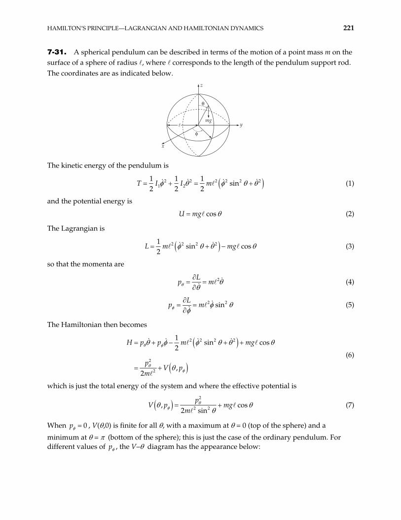
HAMILTON’S PRINCIPLE—LAGRANGIAN AND HAMILTONIAN DYNAMICS 221
7-31. A spherical pendulum can be described in terms of the motion of a point mass m on the surface of a sphere of radius , where corresponds to the length of the pendulum support rod. The coordinates are as indicated below.
"
!
ymg
x
z
The kinetic energy of the pendulum is
2 2 2 2 21 2
1 1 1sin
2 2 2I m 2T I (1)
and the potential energy is
cosU mg (2)
The Lagrangian is
2 2 2 21sin cos
2L m mg (3)
so that the momenta are
2Lp m (4)
2 2sinL
p m (5)
The Hamiltonian then becomes
2 2 2 2
2
2
1sin cos
2
,2
H p p m mg
pV p
m
(6)
which is just the total energy of the system and where the effective potential is
2
2 2,2 sin
pV p mg
mcos (7)
When 0p , V( ,0) is finite for all , with a maximum at = 0 (top of the sphere) and a
minimum at = (bottom of the sphere); this is just the case of the ordinary pendulum. For different values of p , the V– diagram has the appearance below:
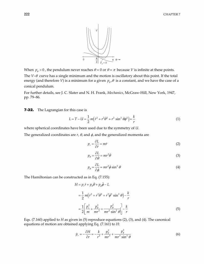
222 CHAPTER 7
V
P! = 00 ((
2"
When 0p , the pendulum never reaches = 0 or = because V is infinite at these points.
The V– curve has a single minimum and the motion is oscillatory about this point. If the total energy (and therefore V) is a minimum for a given p , is a constant, and we have the case of a conical pendulum.
For further details, see J. C. Slater and N. H. Frank, Mechanics, McGraw-Hill, New York, 1947, pp. 79–86.
7-32. The Lagrangian for this case is
2 2 2 2 2 21sin
2k
U m r r rr
L T (1)
where spherical coordinates have been used due to the symmetry of U.
The generalized coordinates are r, , and , and the generalized momenta are
rL
p mrr
(2)
2Lp mr (3)
2 2sinL
p mr (4)
The Hamiltonian can be constructed as in Eq. (7.155):
2 2 2 2 2 2
22 2
2 2 2
1sin
2
12 sin
r
r
H p r p p L
km r r r
r
pp p km mr mr r
(5)
Eqs. (7.160) applied to H as given in (5) reproduce equations (2), (3), and (4). The canonical equations of motion are obtained applying Eq. (7.161) to H:
22
2 3 3 2sinr
ppH kp
r r mr mr (6)
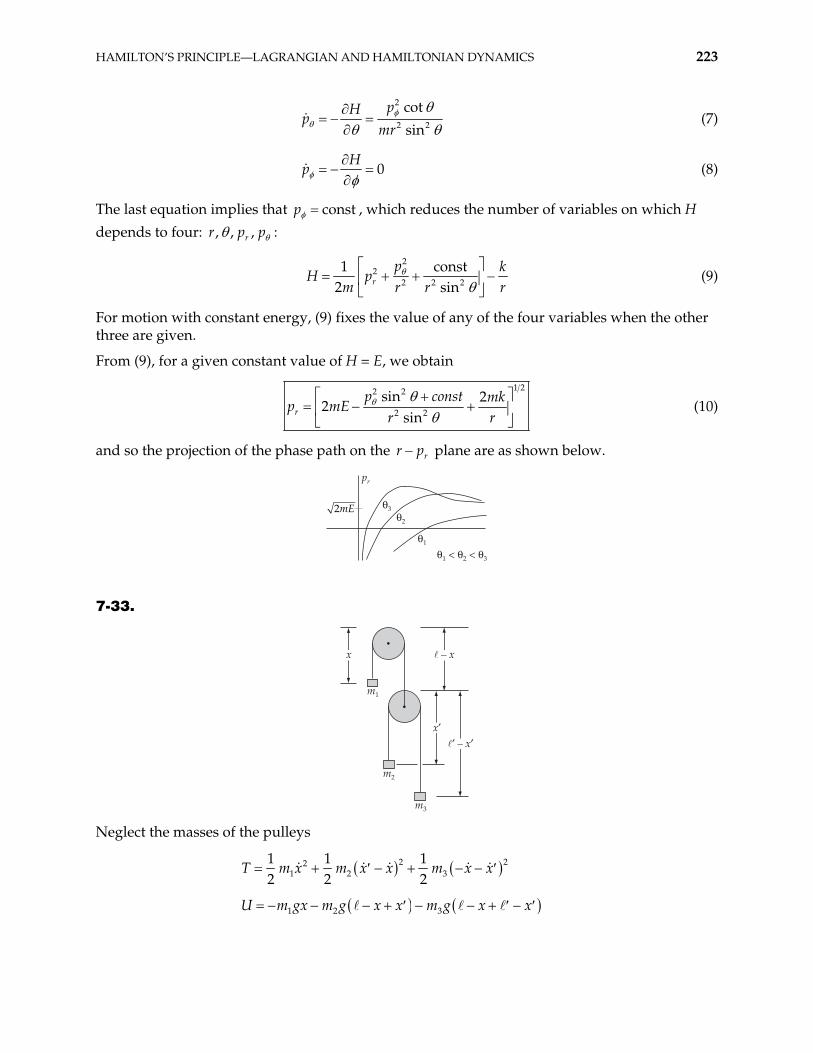
HAMILTON’S PRINCIPLE—LAGRANGIAN AND HAMILTONIAN DYNAMICS 223
2
2 2
cotsin
pHp
mr (7)
0H
p (8)
The last equation implies that constp , which reduces the number of variables on which H depends to four: , , ,rr p p :
2
22 2 2
1 const2 sinr
p kH p
m r r r (9)
For motion with constant energy, (9) fixes the value of any of the four variables when the other three are given.
From (9), for a given constant value of H = E, we obtain
1 22 2
2 2
sin 22
sinrp const mk
Er r
p m (10)
and so the projection of the phase path on the r rp plane are as shown below.
pr
"3"2
"1
"1 < "2 < "3
2mE
7-33.
m1
m2
m3
x&
x
Neglect the masses of the pulleys
2 221 2 3
1 1 12 2 2
x m x x m x xT m
1 2 3m gx m g x x m g x xU
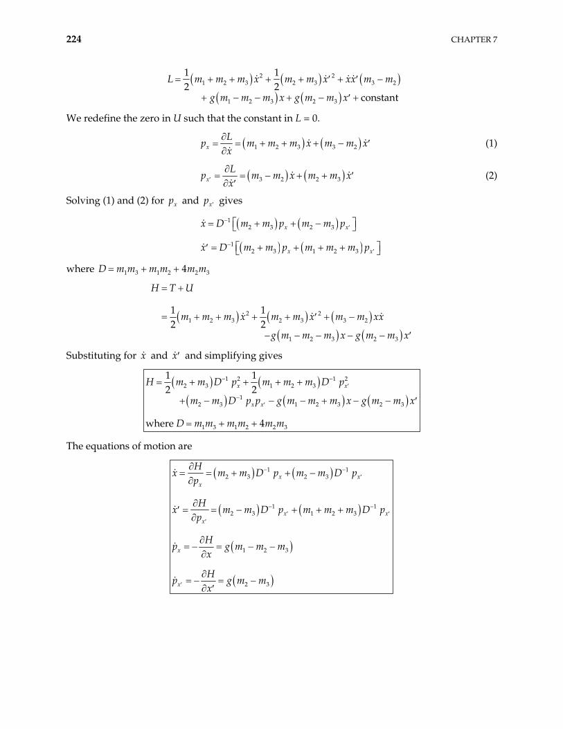
224 CHAPTER 7
2 2
1 2 3 2 3 3 2
1 2 3 2 3
1 1
constant
m m x m m x xx m m
g m m m x g m m x2 2
L m
We redefine the zero in U such that the constant in L = 0.
1 2 3 3 2xL
p m m m x m m xx
(1)
3 2 2 3xL
p m m x m m xx
(2)
Solving (1) and (2) for and gives xp xp
12 3 2 3x xx D m m p m m p
12 3 1 2 3x xx D m m p m m m p
where D m 1 3 1 2 2 34m m m m m
2 21 2 3 2 3 3 2
1 2 3 2 3
1 12 2
H T U
m m m x m m x m m xx
g m m m x g m m x
Substituting for and and simplifying gives x x
1 2 1 22 3 1 2 3
12 3 1 2 3 2 3
1 3 1 2 2 3
1 12 2
where 4
x x
x x
H m m D p m m m D p
m m D p p g m m m x g m m x
D m m m m m m
The equations of motion are
1 12 3 2 3
1 12 3 1 2 3
1 2 3
2 3
x xx
x xx
x
x
Hx m m D p m m D p
p
Hx m m D p m m m D
p
Hp g m m m
x
Hp g m m
x
p
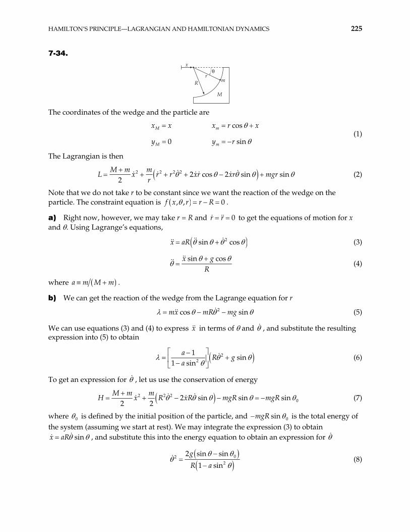
HAMILTON’S PRINCIPLE—LAGRANGIAN AND HAMILTONIAN DYNAMICS 225
7-34.
x
Rr
m
M
"
The coordinates of the wedge and the particle are
cos
0 s
M m
M m
x x x r
y y r in
x (1)
The Lagrangian is then
2 2 2 2 2 cos 2 sin sin2
M m mL x r r xr xr mgr
r (2)
Note that we do not take r to be constant since we want the reaction of the wedge on the particle. The constraint equation is , , 0f x r r R .
a) Right now, however, we may take r = R and 0r r to get the equations of motion for x and . Using Lagrange’s equations,
2sin cosx aR (3)
sin cosx g
R (4)
where a m M m .
b) We can get the reaction of the wedge from the Lagrange equation for r
2cos sinmx mR mg (5)
We can use equations (3) and (4) to express in terms of and x , and substitute the resulting expression into (5) to obtain
22
1sin
1 sina
R ga
(6)
To get an expression for , let us use the conservation of energy
2 2 202 sin sin sin
2 2M m m
H x R xR mgR mgR (7)
where 0 is defined by the initial position of the particle, and 0sinmgR is the total energy of the system (assuming we start at rest). We may integrate the expression (3) to obtain
siR nx a , and substitute this into the energy equation to obtain an expression for
022
2 sin sin
1 sin
g
R a (8)
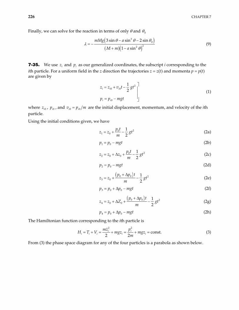
226 CHAPTER 7
Finally, we can solve for the reaction in terms of only and 0
3
022
3 sin sin 2 sin
1 sin
mMg a
M m a (9)
7-35. We use iz and as our generalized coordinates, the subscript i corresponding to the ith particle. For a uniform field in the z direction the trajectories z = z(t) and momenta p = p(t) are given by
ip
2
0 0
0
12i i i
i i
z z v t gt
p p mgt
(1)
where 0iz , , and 0ip 0 0i iv p m are the initial displacement, momentum, and velocity of the ith particle.
Using the initial conditions given, we have
201 0
12
p tz z
mgt
t
(2a)
1 0p p mg (2b)
202 0 0
12
p tz z z g
mt
t
(2c)
2 0p p mg (2d)
0 0 23 0
12
p p tz z
mgt
t
(2e)
3 0 0p p p mg (2f)
0 0 24 0 0
12
p p tz z Z g
mt
t
(2g)
4 0 0p p p mg (2h)
The Hamiltonian function corresponding to the ith particle is
22
const.2 2
iii i i i i
pmzV mgz mgz
mH T (3)
From (3) the phase space diagram for any of the four particles is a parabola as shown below.
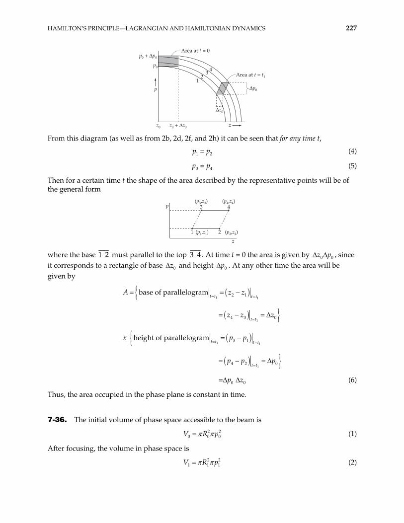
HAMILTON’S PRINCIPLE—LAGRANGIAN AND HAMILTONIAN DYNAMICS 227
p0 + )p0
z0 + )z0
p0
Area at t = 0
Area at t = t1
)p0
z0
)z0
p
z
12
3 4
From this diagram (as well as from 2b, 2d, 2f, and 2h) it can be seen that for any time t,
1p p2 (4)
3p p4 (5)
Then for a certain time t the shape of the area described by the representative points will be of the general form
p
z
1 2
3 4
(p1,z1) (p2,z2)
(p3,z3) (p4,z4)
where the base 1 must parallel to the top 2 3 4 . At time t = 0 the area is given by 0 0z p , since it corresponds to a rectangle of base 0z and height 0p . At any other time the area will be given by
1 1
1
1 1
1
2 1
4 3 0
3 1
4 2 0
0 0
base of parallelogram
height of parallelogram
=
t t t t
t t
t t t t
t t
A z z
z z z
x p p
p p p
p z (6)
Thus, the area occupied in the phase plane is constant in time.
7-36. The initial volume of phase space accessible to the beam is
20 0V R p2
0 (1)
After focusing, the volume in phase space is
2 21 1V R p1 (2)
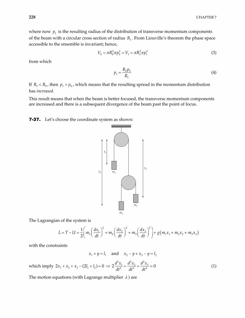
228 CHAPTER 7
where now is the resulting radius of the distribution of transverse momentum components of the beam with a circular cross section of radius . From Liouville’s theorem the phase space accessible to the ensemble is invariant; hence,
1p
1R
2 2 20 0 0 1 1V R p V R p2
1 (3)
from which
0 01
1
R pp
R (4)
If , then , which means that the resulting spread in the momentum distribution has increased.
1R R0 01p p
This result means that when the beam is better focused, the transverse momentum components are increased and there is a subsequent divergence of the beam past the point of focus.
7-37. Let’s choose the coordinate system as shown:
x1
m1
m2
m3
x3x2
The Lagrangian of the system is
22 2
31 21 2 3 1 1 2 2
12
dxdx dxL T U m m m g m x m x m x
dt dt dt 3 3
1 2
with the constraints
and 1x y l 2 3x y x y l
which imply 22 2
31 21 2 3 1 2 2 2 22 (2 ) 0 2
d xd x d xx x x l l
dt dt dt0 (1)
The motion equations (with Lagrange multiplier ) are
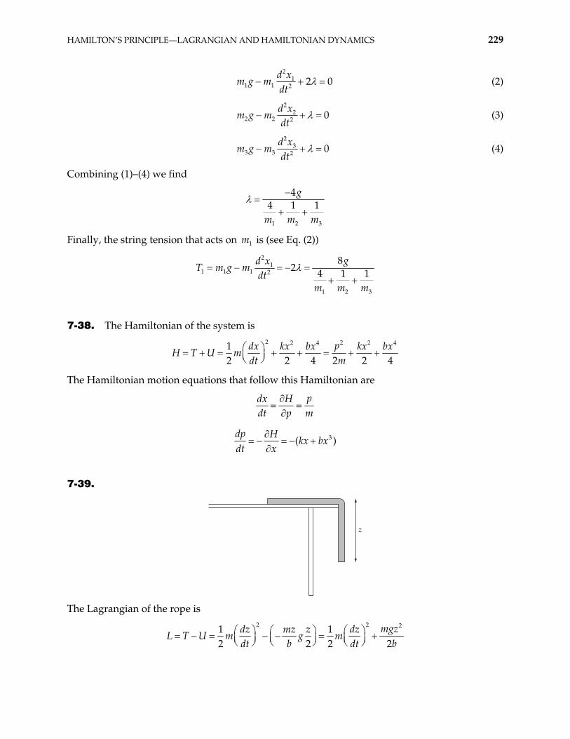
HAMILTON’S PRINCIPLE—LAGRANGIAN AND HAMILTONIAN DYNAMICS 229
2
11 1 2 2
d xm g m
dt0 (2)
2
22 2 2 0
d xm g m
dt (3)
2
33 3 2 0
d xm g m
dt (4)
Combining (1)–(4) we find
1 2
44 1 1
g
m m m3
Finally, the string tension that acts on m is (see Eq. (2)) 1
2
11 1 1 2
1 2
82 4 1 1
gd xg m
dtm m m3
T m
7-38. The Hamiltonian of the system is
2 22 4 21
2 2 4 2 2pdx kx bx kx bx
U mdt m
4
4H T
The Hamiltonian motion equations that follow this Hamiltonian are
pdx H
dt p m
3( )dp H
kx bxdt x
7-39.
z
The Lagrangian of the rope is
2 2 21 1
2 2 2mgzdz mz z dz
U m g mdt b dt b2
L T
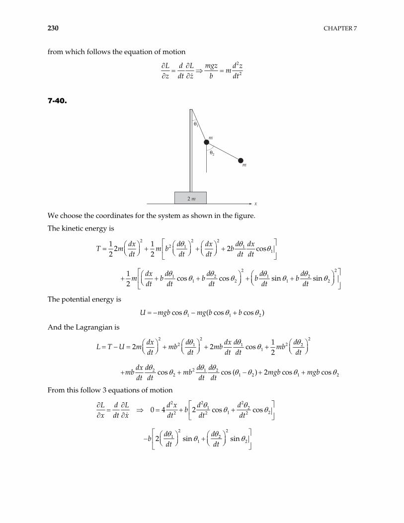
230 CHAPTER 7
from which follows the equation of motion
2
2
mgzL d L d zm
z dt z b dt
7-40.
m
m
2 mx
"2
"1
We choose the coordinates for the system as shown in the figure.
The kinetic energy is
22 22 1 1
1
2 21 2 1 2
1 2 1
1 12 2 cos
2 2
1cos cos sin sin
2
d ddx dx dxT m m b b
dt dt dt dt dt
d d d ddxm b b b b
dt dt dt dt dt 2
2
The potential energy is
U m 1 1cos ( cos cos )gb mg b b
And the Lagrangian is
2 222 21 1 2
1
22 1 22 1 2 1
12 2 cos
2
cos cos ( ) 2 cos cos
d d ddx dxL T U m mb mb mb
dt dt dt dt dt
d d ddxmb mb mgb mgb
dt dt dt dt 2
From this follow 3 equations of motion
2 221 2
1 22 2 2
2 21 2
1 2
0 4 2 cos cos
2 sin sin
d dL d L d xb
x dt x dt dt dt
d db
dt dt
HAMILTON’S PRINCIPLE—LAGRANGIAN AND HAMILTONIAN DYNAMICS 231
2 221 2
1 12 2 21 1
22
1 2
2 sin 2 2 cos cos( )
sin( )
d dL d L d xg b b
dt dt dt dt
db
dt
1 2
2 2
22 222 1 1
2 2 1 22 2 2sin cos cos ( ) sin ( )
L d Ldt
d d dd xg b b b
dt dt dt dt 1 2
7-41. For small angle of oscillation we have
2 2
21 12 2
d db m
dt dtb
T m and U m cosgb
So the Lagrangian reads
2 2
21 1cos
2 2d db
U mb m mgbdt dt
L T
from which follow 2 equations of motion
2 2
2cosL d L d d b d
b gb dt dt dt dtb
2 2
2 22 2sin 2 2
L d L db d d d dmgb mb mb mb mb
dt dt dt dt dt dt

232 CHAPTER 7
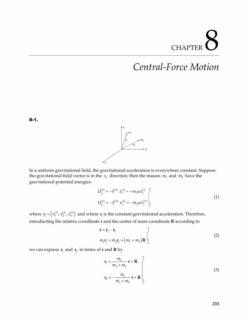
CHAPTER 8 Central-Force Motion
8-1.
x3
m2
m1
x2
r1
r2
x1 In a uniform gravitational field, the gravitational acceleration is everywhere constant. Suppose the gravitational field vector is in the x direction; then the masses and have the gravitational potential energies:
1 1m 2m
1 1 1 11 1 1
2 2 2 21 2 1
g
g
U F x m x
U F x m x (1)
where 1 1 11 1 2 3, ,x x xr and where is the constant gravitational acceleration. Therefore,
introducting the relative coordinate r and the center of mass coordinate R according to
1 2
1 1 2 2 1 2m m m m
r r r
r r R (2)
we can express r and r in terms of r and R by 1 2
21
1 2
12
1 2
mm m
mm m
r r
r r
R
R
(3)
233
234 CHAPTER 8
which differ from Eq. (8.3) in the text by R. The Lagrangian of the two-particle system can now be expressed in terms of r and R:
2 2 1 21 1 2 2
2 2
2 11 2
1 2 1 2
2 11 2
1 2 1 2
1 12 2
1 12 2
g gL m m U U U
m mm m U r
m m m mm m
m x X m xm m m m
X
r r r
r R r R (4)
where x and X are the components of r and R, respectively. Then, (4) becomes 1x
222 22 1
1 2 11 2 1 2
1 2 1 21 2
1 2
1 1 12
m mL m m m m
m m m mm m m m
U r x m m Xm m
r r 2 R2 2 (5)
Hence, we can write the Lagrangian in the form
22
1 2 1 21 12 2
r m m m mL U Xr R (6)
where is the reduced mass:
1 2
1 2
m mm m
(7)
Therefore, this case is reducible to an equivalent one-body problem.
8-2. Setting 1u r , Eq. (8.38) can be rewritten as
2
2 22 2
duE k u u
(1)
where we have used the relation 21du r dr . Using the standard form of the integral [see Eq. (E.8c), Appendix E]:
1
2 2
1 2sin const.
4
dx ax baax bx c b ac
(2)
we have
2
1
2
2 2
2 2
const. sin2 8
krk E
(3)
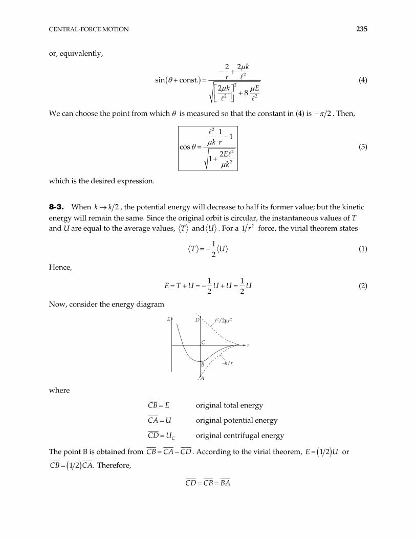
CENTRAL-FORCE MOTION 235
or, equivalently,
2
2
2 2
2 2
sin const.2 8
krk E
(4)
We can choose the point from which is measured so that the constant in (4) is 2 . Then,
2
2
2
1 1cos
21
k r
Ek
(5)
which is the desired expression.
8-3. When 2k k , the potential energy will decrease to half its former value; but the kinetic energy will remain the same. Since the original orbit is circular, the instantaneous values of T and U are equal to the average values, T and U . For a 2r1 force, the virial theorem states
12
T U (1)
Hence,
1 12 2
E T U U U U (2)
Now, consider the energy diagram
E D
C
A
r
–k/rB
where
CB E original total energy
CA U original potential energy
CCD U original centrifugal energy
The point B is obtained from CB CA CD . According to the virial theorem, 1 2E U or
1 2 .CB CA Therefore,
CD CB BA
236 CHAPTER 8
Hence, if U suddenly is halved, the total energy is raised from B by an amount equal to 1 2 CA
or by CB . Thus, the total energy point is raised from B to C; i.e., E(final) = 0 and the orbit is parabolic.
8-4. Since the particle moves in a central, inverse-square law force field, the potential energy is
k
Ur
(1)
so that the time average is
0
1 kU
rdt (2)
Since this motion is a central motion, the angular momentum is a constant of motion. Then,
(3) 2 .r const
from which
2r
dt d (4)
Therefore, (2) becomes
2 22
0 0
1 k r kU d
rrd (5)
Now, substituting 1 cosr and 3 22 a , (5) becomes
2
3 20
12 1 cosk
Ua
d (6)
where a is the semimajor axis of the ellipse. Using the standard integral [see Eq. (E.15), Appendix E],
2
20
11 cos 1
d2
(7)
and the relation,
21a (8)
(6) becomes
k
Ua
(9)
The kinetic energy is
CENTRAL-FORCE MOTION 237
2
22
12 2
T rr
(10)
and the time average is
2
23
0 0
1 12
kT T dt Tr
ad (11)
Part of this integral is trivial,
2 2
23
0
12 2
kT rr d
a (12)
To evaluate the integral above, substitute the expression for r and make a change of variable
2 22 2 12 2
22
0 0 1
sin 12 2 11 cos
d xrr d
x 2
dx1 1 (13)
The reader is invited to evaluate this integral in either form. The solution presented here is to integrate by parts twice, which gives a third integral that can be looked up in a table:
1
1 12 2
2 21 11
1 1 111 1 1
x dx x dxxxx x x
(14)
1 11 1
211
sin sin11 1
x x x dx x
x (15)
1
1 12 2
1
1 11 2sin tan
1 11
xx
x (16)
2 2
11
1 (17)
Substituting this into (13) and then into (12), we obtain the desired answer,
2k
Ta
(18)
This explicitly verifies the virial theorem, which states that for an inverse-square law force,
12
T U (19)
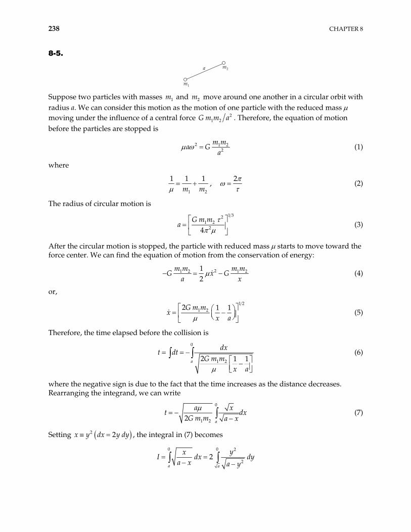
238 CHAPTER 8
8-5.
a
m1
m2
Suppose two particles with masses and move around one another in a circular orbit with radius a. We can consider this motion as the motion of one particle with the reduced mass moving under the influence of a central force
1m 2m
21 2G m m a . Therefore, the equation of motion
before the particles are stopped is
2 1 22
m ma G
a (1)
where
1 2
1 1 1m m
, 2
(2)
The radius of circular motion is
1 32
1 224
G m ma (3)
After the circular motion is stopped, the particle with reduced mass starts to move toward the force center. We can find the equation of motion from the conservation of energy:
21 2 1 212
m m m mG x G
a x (4)
or,
1 2
1 22 1 1G m mx
x a (5)
Therefore, the time elapsed before the collision is
0
1 22 1 1a
dxt dt
G m mx a
(6)
where the negative sign is due to the fact that the time increases as the distance decreases. Rearranging the integrand, we can write
0
1 22 a
a xt
G m m a xdx (7)
Setting 2 2x y dx y dy , the integral in (7) becomes
0 0 2
22
a a
yxI dx
a x a ydy
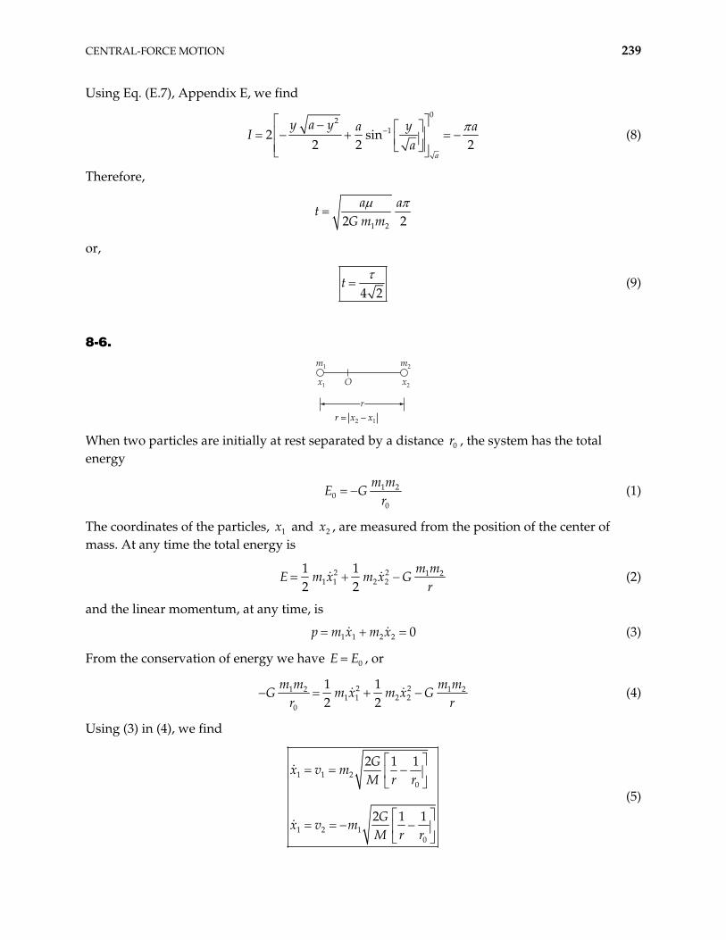
CENTRAL-FORCE MOTION 239
Using Eq. (E.7), Appendix E, we find
02
12 sin2 2
a
y a y ya aa 2
I (8)
Therefore,
1 22 2
a at
G m m
or,
4 2
t (9)
8-6.
m1 m2
x1 x2O
rr x x= !2 1
When two particles are initially at rest separated by a distance , the system has the total energy
0r
1 20
0
m mE G
r (1)
The coordinates of the particles, and , are measured from the position of the center of mass. At any time the total energy is
1x 2x
2 2 1 21 1 2 2
1 12 2
m mE m x m x G
r (2)
and the linear momentum, at any time, is
1 1 2 2 0p m x m x (3)
From the conservation of energy we have E 0E , or
2 21 2 1 21 1 2 2
0
1 12 2
m m m mG m x m x G
r r (4)
Using (3) in (4), we find
1 1 20
1 2 10
2 1 1
2 1 1
Gx v m
M r r
Gx v m
M r r
(5)
240 CHAPTER 8
8-7. Since F r kr is a central force, angular momentum is conserved and the areal velocity, 2dA dt , is trivially constant (see Section 8.3). In order to compute U , we start with
2
22
2
drdt
E Ur
(1)
and
2
2kr
U (2)
The time average of the potential energy becomes
max
min
0
3
4 22
1
22 2
2 2
r
r
U U dt
kr dr
krEr
(3)
Substituting
2 12
r x dr dxr
(4)
(4) becomes
2max
2min 2
22 22 2
r
r
x dxkU
kEx x
(5)
Using the integrals in Eqs. (E.9) and (E.8c), Appendix E,
2 1
2 2
1sin
2 4
x dx b axax bx c
a a aax bx c b ac
2 b (6)
(5) becomes
max
min
1 2 2 21 4
1 222
2 2sin
2 2 2 2
r
r
k E E kr kU r
k k kkE
2Er (7)
But and were originally defined as the roots of maxr minr2
22E U
r. Hence, the second term
vanishes at both limits of integration. On the other hand,
CENTRAL-FORCE MOTION 241
max
min
max
min
2
2
24 2
22
2
2
2 2
r
r
r
r
dr
E Ur
rdr
k r Er
(8)
or, using (5),
2max
2min
max
min
22
1 2 21
1 222
22 2
2sin
2
r
r
r
r
dx
kx Ex
E krk kE
(9)
Using (9) to substitute for in (7), we have
2E
U (10)
Now,
2E
T E U (11)
The virial theorem states:
1
2n
T U when U k 1nr (12)
In our case n = 1, therefore,
2E
T U (13)
8-8. The general expression for (r) is [see Eq. (8.17)]
2
2
222
r drr
E Ur
(1)
where 2 2r dr krU k in the present case. Substituting 2x r and dx = 2r dr into (1), we
have
242 CHAPTER 8
2
2 2
12 2 1
dxr
k Ex x x (2)
Using Eq. (E.10b), Appendix E,
1
2
1 2sin
4
dx bx ccx ax bx c x b ac2
(3)
and expressing again in terms of r, we find
22
102 2
24 2
11
sin2
E rr
E kr
(4)
or,
2
0 22
2 2
1n 2
1 1
Erk k
E E
2si (5)
In order to interpret this result, we set
2
2
2
1k
E
E
(6)
and specifying 0 4 , (5) becomes
2 1 cos 2r
(7)
or,
2 2 2 2cos sinr r (8)
Rewriting (8) in x-y coordinates, we find
2 2 2 2x y x y (9)
or,
22
1
1 1
yx (10)
Since a > 0, > 1 from the definition, (10) is equivalent to
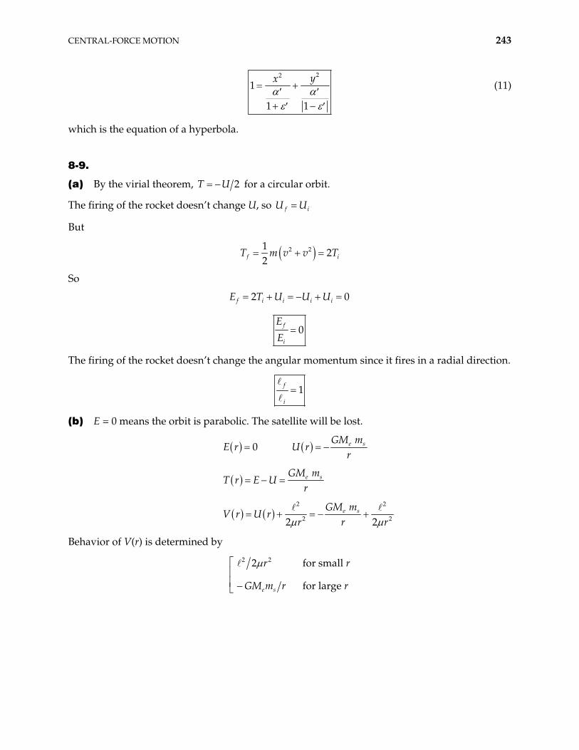
CENTRAL-FORCE MOTION 243
22
1
1 1
yx (11)
which is the equation of a hyperbola.
8-9.
(a) By the virial theorem, 2UT for a circular orbit.
The firing of the rocket doesn’t change U, so f iU U
But
2 212
2f iT m v v T
So
2 0f i i i iE T U U U
0f
i
E
E
The firing of the rocket doesn’t change the angular momentum since it fires in a radial direction.
1f
i
(b) E = 0 means the orbit is parabolic. The satellite will be lost.
0 e sGM mE r U r
r
e sGM mT r E U
r
2 2
2 22 2e sGM m
V r U rr r r
Behavior of V(r) is determined by
2 22 for small
for large e s
r r
GM m r r
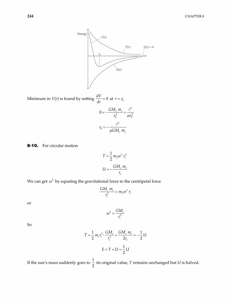
244 CHAPTER 8
EnergyV(r)
U(r)
T(r) E(r) = 0
r0
Minimum in V(r) is found by setting 0dVdr
at 0r r
2
2 30 0
0 e sGM mr r
2
0e s
rGM m
8-10. For circular motion
2 212 e eT m r
s e
e
GM mU
r
We can get 2 by equating the gravitational force to the centripetal force
22s e
e ee
GM mm r
r
or
23
s
e
GMr
So
23
1 12 2
s ese e
e e
GM mGMT m r
r r 2U
12
E T U U
If the sun’s mass suddenly goes to 12
its original value, T remains unchanged but U is halved.
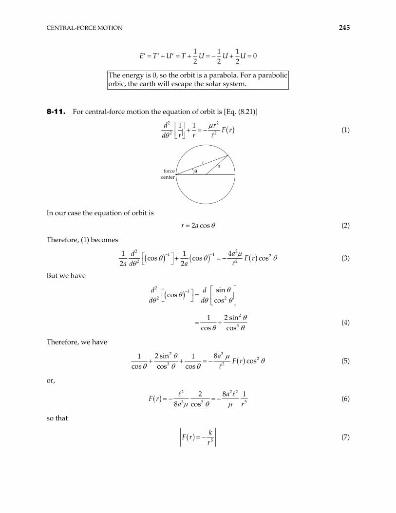
CENTRAL-FORCE MOTION 245
1 1 1
02 2 2
U T U U UE T
Tor
he energy is 0, so the orbit is a parabola. For a parabolicbic, the earth will escape the solar system.
8-11. For central-force motion the equation of orbit is [Eq. (8.21)]
2 2
2 2
1 1d rF r
d r r (1)
forcecenter
ra
"
In our case the equation of orbit is
2 cosr a (2)
Therefore, (1) becomes
2 2
1 1 22
4cos cos cos
2 2d
F ra d a 2
a1 1 (3)
But we have
21
2 2
2
3
sincos
cos
2 sin1cos cos
d dd d
(4)
Therefore, we have
2 3
23 2
2 sin 81 1cos
cos cos cosa
F r (5)
or,
2 2
3 5
2 88 cos
aF r
a r
2
5
1 (6)
so that
5
kF r
r (7)
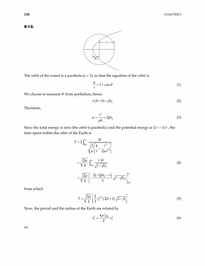
246 CHAPTER 8
8-12.
#re
re
The orbit of the comet is a parabola ( = 1), so that the equation of the orbit is
1 cosr
(1)
We choose to measure from perihelion; hence
0 Er r (2)
Therefore,
2
2 Erk (3)
Since the total energy is zero (the orbit is parabolic) and the potential energy is U k r , the time spent within the orbit of the Earth is
2
2
22
2
2
2 223
E
E
E
E
E
E
r
r
r
rE
rE
Er
drT
kr r
r drk r r
r rr r
k
(4)
from which
3 22 22 1 1
3 ET rk
(5)
Now, the period and the radius of the Earth are related by
2
2 4 EE r
k3
E (6)
or,
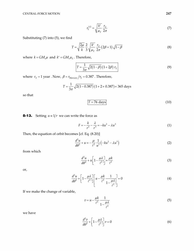
CENTRAL-FORCE MOTION 247
3 2
2E
EE
kr (7)
Substituting (7) into (5), we find
2 2
2 1 13 2
E
E
kT
k (8)
where sk GM and s Ek GM . Therefore,
1
2 1 1 23 ET (9)
where 1 yearE . Now, Mercury 0.387Er r . Therefore,
1
2 1 0.387 1 2 0.387 365 days3
T
so that
76 daysT (10)
8-13. Setting 1u we can write the force as r
22 3
k 3F ku ur r
(1)
Then, the equation of orbit becomes [cf. Eq. (8.20)]
2
22 2 2
1d uu ku
d u3u (2)
from which
2
2 21d u k
ud 2 (3)
or,
2
2 2 2
2
11
1
d u ku
d0 (4)
If we make the change of variable,
2
2
1
1
kv u (5)
we have
2
2 21d v
vd
0 (6)
248 CHAPTER 8
or,
2
22 0
d vv
d (7)
where 2 21 . This equation gives different solutions according to the value of . Let us consider the following three cases:
i) 2 :
For this case and the solution of (7) is 2 0
cosv A
By proper choice of the position = 0, the integration constant can be made to equal zero. Therefore, we can write
2
1cos
kA
r (9)
When = 1 ( = 0), this equation describes a conic section. Since we do not know the value of the constant A, we need to use what we have learned from Kepler’s problem to describe the motion. We know that for = 0,
2
11 cos
kr
and that we have an ellipse or circle (0 < 1) when E < 1, a parabola ( = 1) when E = 0, and a hyperbola otherwise. It is clear that for this problem, if E 0, we will have some sort of parabolic or hyperbolic orbit. An ellipse should result when E < 0, this being the only bound orbit. When 1, the orbit, whatever it is, precesses. This is most easily seen in the case of the ellipse, where the two turning points do not have an angular separation of . One may obtain most constants of integration (in particular A) by using Equation (8.17) as a starting point, a more formal approach that confirms the statements made here.
ii) 2
For this case and (3) becomes 2 0
2
2
d u kd 2 (10)
so that
22
12
ku
rA B (11)
from which we see that r continuously decreases as increases; that is, the particle spirals in toward the force center.
CENTRAL-FORCE MOTION 249
iii) 2
For this case and the solution (7) is 2 0
2coshv A (12)
may be set equal to zero by the proper choice of the position at which = 0. Then,
22
1cosh
kA
r (13)
Again, the particle spirals in toward the force center.
8-14. The orbit equation for the central-force field is [see Eq. (8.17)]
2 4 2
2
22
dr rE U
d r2 (1)
But we are given the orbit equation:
2r k (2)
from which
2
2 24dr
kd
(3)
Substituting (2) into (3), we have
2
24 4dr r
kd k
kr (4)
From (1) and (4), we find the equation for the potential U:
4 2
2
24
2r
kr E Ur2 (5)
from which
2 2
3
2 12
kU E
r r2
1 (6)
and F r U r . Therefore,
2
4 3
6 1kF r
r r (7)
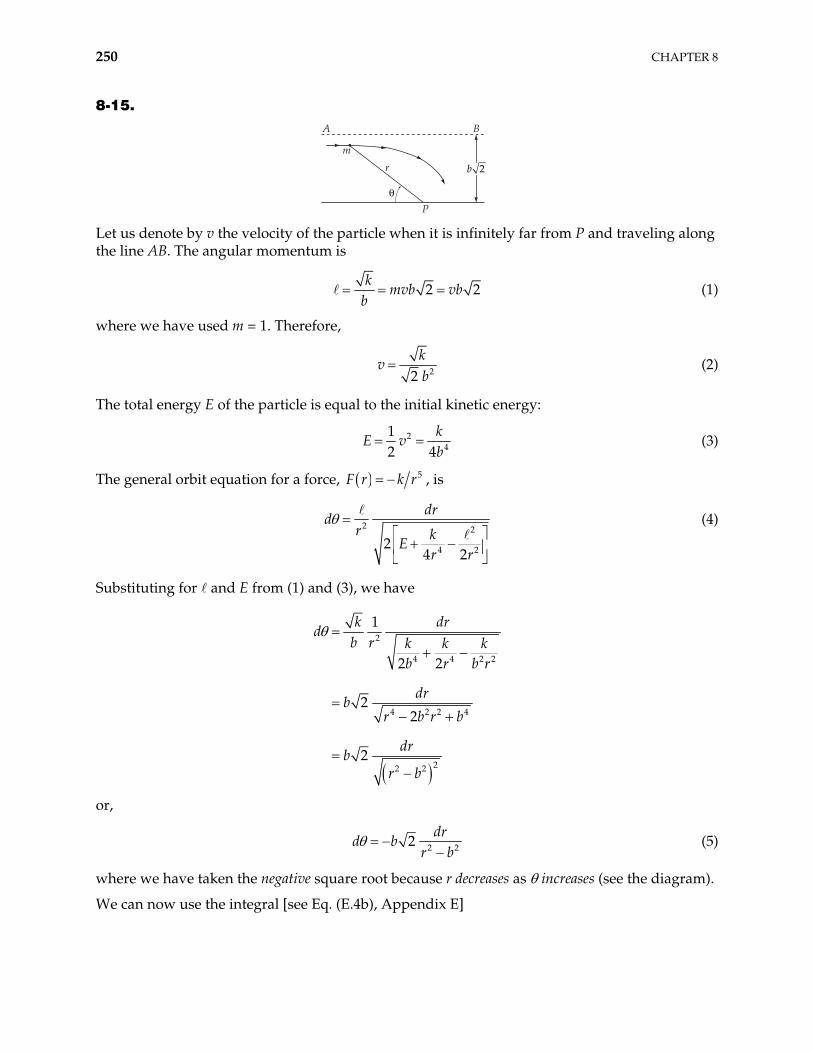
250 CHAPTER 8
8-15.
A B
r
P
m
"
b 2
Let us denote by v the velocity of the particle when it is infinitely far from P and traveling along the line AB. The angular momentum is
2k
mvb vbb
2 (1)
where we have used m = 1. Therefore,
22k
vb
(2)
The total energy E of the particle is equal to the initial kinetic energy:
24
12 4
kE v
b (3)
The general orbit equation for a force, 5F r k r , is
2 2
4 224 2
drd
r kEr r
(4)
Substituting for and E from (1) and (3), we have
2
4 4 2
4 2 2 4
22 2
1
2 2
22
2
k drd
b r k k kb r b r
drb
r b r b
drb
r b
2
or,
22dr
d br b2 (5)
where we have taken the negative square root because r decreases as increases (see the diagram).
We can now use the integral [see Eq. (E.4b), Appendix E]
CENTRAL-FORCE MOTION 251
12 2 2
1coth
dx axa x b ab b
(6)
from which we obtain
102 coth
rb
(7)
or,
0coth2
r b (8)
Now, coth as 0, since r as 0, we must have 0 0 . Thus,
coth 2r b (9)
Notice that r is always greater than b (because coth 1 as ), so that the denominator in (5) never equals zero nor changes sign. Thus, r always decreases as increases. This is, the particle spirals in toward P but never approaches closer than a distance b.
8-16. The total energy of the particle is
E T U (1)
a principle that by no means pushes the philosophical envelope of physical interpretation. The impulse that causes v v + v changes the kinetic energy, not the potential energy. We therefore have
212
E T mv mv v (2)
By the virial theorem, for a nearly circular orbit we have
212
E mv (3)
so that
2E v
E v (4)
where we have written –E since E < 0. The major and minor axes of the orbit are given by
2 2k
a bE E
(5)
Now let us compute the changes in these quantities. For a we have
22 2k k E E
aE E E
a (6)
and for b we have
252 CHAPTER 8
3
12 22 2 2
Eb
EE E EE b (7)
Easily enough, we can show that v v and therefore
2a b E
a b E vv
(8)
8-17. The equation of the orbit is
1 cosr
(1)
from which
1 cos
r (2)
where 2 k and 2
2
21
Emk
. Therefore, the radial distance r can vary from the
maximum value 1 to the minimum value 1 . Now, the angular velocity of the particle is given by
2r (3)
Thus, the maximum and minimum values of become
max 22min
min 22max
1
1
r
r
(4)
Thus,
2
max
min
11
n (5)
from which we find
11
nn
(6)
8-18. Kepler’s second law states that the areal velocity is constant, and this implies that the angular momentum L is conserved. If a body is acted upon by a force and if the angular momentum of the body is not altered, then the force has imparted no torque to the body; thus,
CENTRAL-FORCE MOTION 253
the force must have acted only along the line connecting the force center and the body. That is, the force is central.
Kepler’s first law states that planets move in elliptical orbits with the sun at one focus. This means the orbit can be described by Eq. (8.41):
1 cos with 0r
1 (1)
On the other hand, for central forces, Eq. (8.21) holds:
2 2
2 2
1 1d rF r
d r r (2)
Substituting 1 from (1) into the left-hand side of (2), we find r
22
1r F r
a (3)
which implies, that
2
2F rr
(4)
8-19. The semimajor axis of an orbit is defined as one-half the sum of the two apsidal distances, and [see Eq. (8.44)], so maxr minr
max min 2
1 12 2 1 1
r r1
(1)
This is the same as the semimajor axis defined by Eq. (8.42). Therefore, by using Kepler’s Third Law, we can find the semimajor axis of Ceres in astronomical units:
22
22
4
4
CC
C C
EEE
E
ka
ka (2)
where c sk M mc , and
1 1 1
c sM mc
Here, sM and are the masses of the sun and Ceres, respectively. Therefore, (2) becomes cm
1 32
C s c c
E s e E
a M ma M m
(3)
from which
254 CHAPTER 8
1 3
2
1333, 4808,000 4.6035
333, 480 1C
E
aa
(4)
so that
2.767C
E
aa
(5)
The period of Jupiter can also be calculated using Kepler’s Third Law:
1 223 1 23
23
4
4
JJ
J J Js E
EE sE
E
ak aM m
M m aak
J E
(6)
from which
1 2
3333, 480 15.2028
333, 480 318.35J
E
(7)
Therefore,
11.862J
E
(8)
The mass of Saturn can also be calculated from Kepler’s Third law, with the result
95.3s
e
mm
(9)
8-20. Using Eqs. (8.42) and (8.41) for a and r, we have
44
20
1 cos1cos cos
1a
dtr
(1)
From Kepler’s Second Law, we can find the relation between t and :
2
212 1 cos
dt dA dab ab
(2)
since 21 2dA r d . Therefore, (1) becomes
4 22
242
0
1 1cos cos 1 cos
21
a ad
r ab (3)
It is easily shown that the value of the integral is 2 . Therefore,
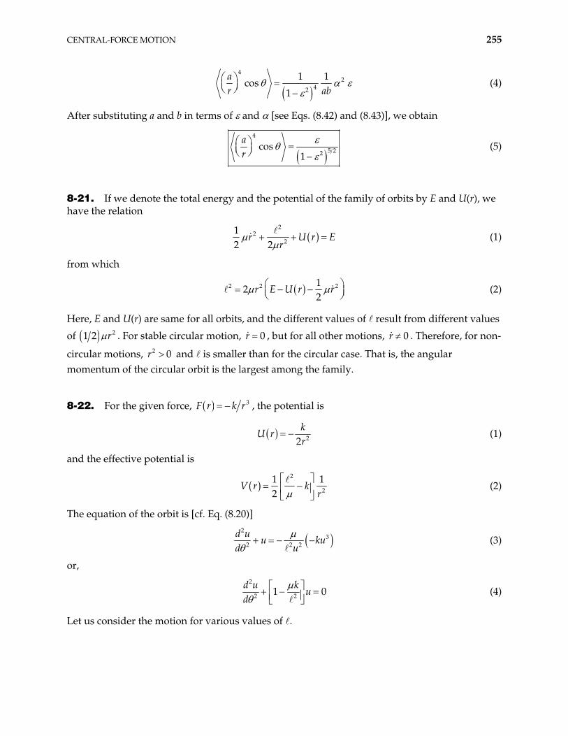
CENTRAL-FORCE MOTION 255
4
242
1 1cos
1
ar ab
(4)
After substituting a and b in terms of and [see Eqs. (8.42) and (8.43)], we obtain
4
5 22cos
1
ar
(5)
8-21. If we denote the total energy and the potential of the family of orbits by E and U(r), we have the relation
2
22
12 2
r U rr
E (1)
from which
2 2 12
2r E U r r2 (2)
Here, E and U(r) are same for all orbits, and the different values of result from different values
of 21 2 r . For stable circular motion, 0r , but for all other motions, 0r . Therefore, for non-
circular motions, and is smaller than for the circular case. That is, the angular momentum of the circular orbit is the largest among the family.
2 0r
8-22. For the given force, 3F r k r , the potential is
22k
U rr
(1)
and the effective potential is
2
2
1 12
V r kr
(2)
The equation of the orbit is [cf. Eq. (8.20)]
2
32 2 2
d uu
d uku (3)
or,
2
2 21d u k
ud
0 (4)
Let us consider the motion for various values of .
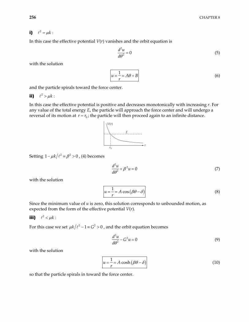
256 CHAPTER 8
i) 2 k :
In this case the effective potential V(r) vanishes and the orbit equation is
2
2 0d ud
(5)
with the solution
1
u Ar
B (6)
and the particle spirals toward the force center.
ii) 2 k :
In this case the effective potential is positive and decreases monotonically with increasing r. For any value of the total energy E, the particle will approach the force center and will undergo a reversal of its motion at ; the particle will then proceed again to an infinite distance. 0r r
V(r)
E
rr0
Setting 2 2k1 , (4) becomes 0
2
22 0
d uu
d (7)
with the solution
1
cosu Ar
(8)
Since the minimum value of u is zero, this solution corresponds to unbounded motion, as expected from the form of the effective potential V(r).
iii) 2 k :
For this case we set 2 21k G 0 , and the orbit equation becomes
2
22 0
d uG u
d (9)
with the solution
1
coshu Ar
(10)
so that the particle spirals in toward the force center.
CENTRAL-FORCE MOTION 257
In order to investigate the stability of a circular orbit in a 3r1 force field, we return to Eq. (8.83)
and use 3g r k r . Then, we have
2
32 3 31 1
k
x x3x (11)
or,
2
33
10
1x k
x (12)
Since 0r pr , Eq. (8.87) shows that 2k . Therefore, (12) reduces to
0x (13)
so that the perturbation x increases uniformly with the time. The circular orbit is therefore not stable.
We can also reach the same conclusion by examining the basic criterion for stability, namely, that
2
20 and 0r r
V Vr r
The first of these relations requires 2k while the second requires 2 k . Since these requirements cannot be met simultaneously, no stable circular orbits are allowed.
8-23. Start with the equation of the orbit:
1 cosr
(1)
and take its time derivative
2 sin sinrr r2 (2)
Now from Equation (8.45) and (8.43) we have
2
2 2
1
aab (3)
so that from (2)
max 2
2
1
ar (4)
as desired.
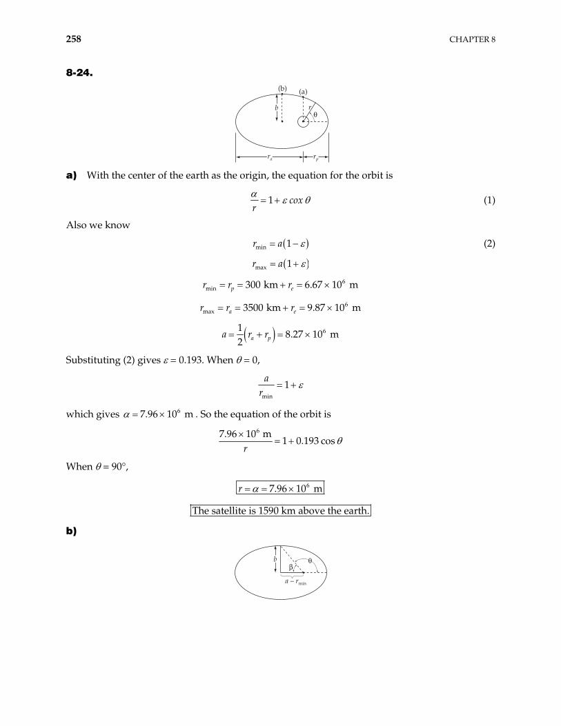
258 CHAPTER 8
8-24.
r
(b) (a)
"b
ra rp a) With the center of the earth as the origin, the equation for the orbit is
1 coxr
(1)
Also we know
min 1r a (2)
max 1r a
6min 300 km 6.67 10 mp er r r
r r 6max 3500 km 9.87 10 ma er
618.27 10 m
2 a pa r r
Substituting (2) gives = 0.193. When = 0,
min
1a
r
which gives . So the equation of the orbit is 67.96 10 m
67.96 10 m
1 0.193 cosr
When = 90°,
67.96 10 mr
T he satellite is 1590 km above the earth.
b)
b
a – rmin
#"
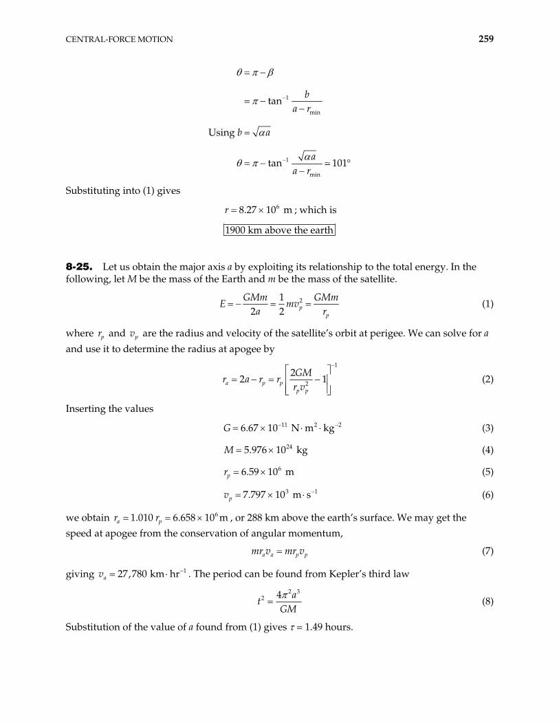
CENTRAL-FORCE MOTION 259
1
min
1
min
tan
Using
tan 101
ba r
b a
aa r
Substituting into (1) gives
; which is 68.27 10 mr
1900 km above the earth
8-25. Let us obtain the major axis a by exploiting its relationship to the total energy. In the following, let M be the mass of the Earth and m be the mass of the satellite.
212 2 p
p
GMm GMmE mv
a r (1)
where pr and pv are the radius and velocity of the satellite’s orbit at perigee. We can solve for a and use it to determine the radius at apogee by
1
2
22a p p
p p
GMr a r r
r v1 (2)
Inserting the values
11 2 26.67 10 N m kgG (3)
(4) 245.976 10 kgM
(5) 66.59 10 mpr
37.797 10 m spv 1 (6)
we obtain , or 288 km above the earth’s surface. We may get the speed at apogee from the conservation of angular momentum,
61.010 6.658 10 ma pr r
a a p pmr v mr v (7)
giving . The period can be found from Kepler’s third law 127,780 km hrav
2 3
2 4 at
GM (8)
Substitution of the value of a found from (1) gives = 1.49 hours.
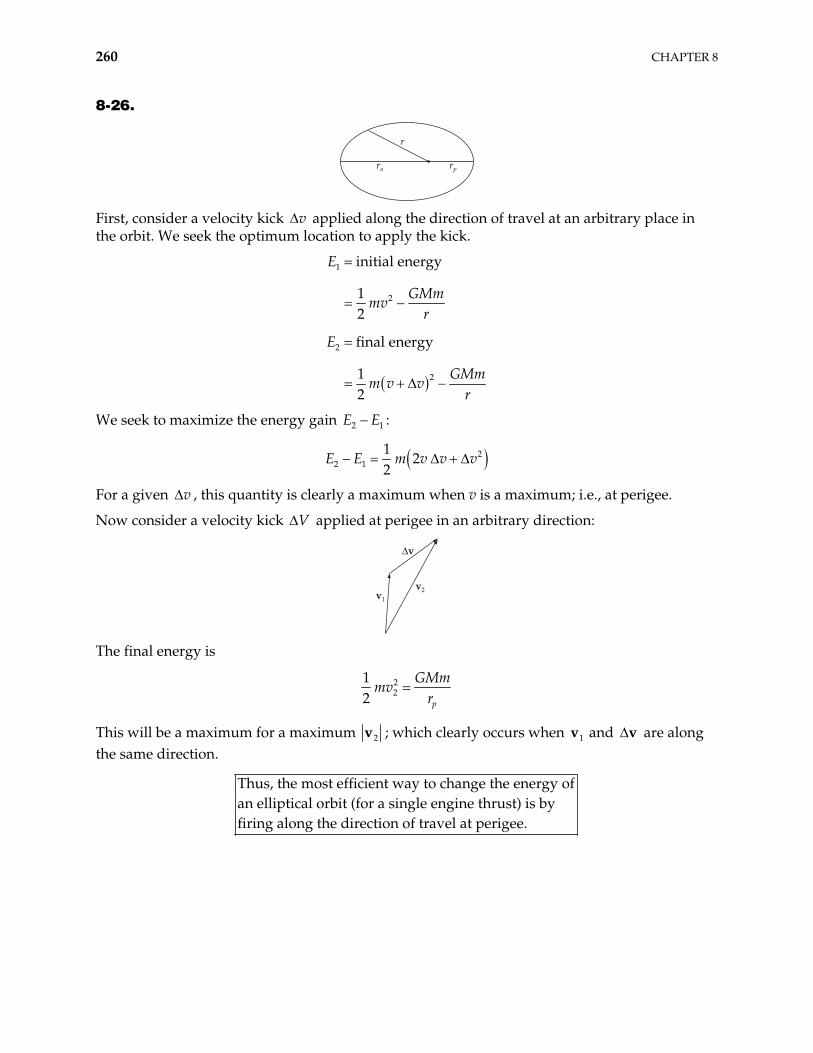
260 CHAPTER 8
8-26.
r
ra rp
First, consider a velocity kick applied along the direction of travel at an arbitrary place in the orbit. We seek the optimum location to apply the kick.
v
1
2
2
2
initial energy
12
final energy
12
E
GMmmv
r
E
GMmm v v
r
We seek to maximize the energy gain E E2 1 :
22 1
12
2E E m v v v
For a given , this quantity is clearly a maximum when v is a maximum; i.e., at perigee. v
Now consider a velocity kick applied at perigee in an arbitrary direction: V
$v
v2v1
The final energy is
22
12 p
GMmmv
r
This will be a maximum for a maximum 2v ; which clearly occurs when and are along the same direction.
1v v
Thus, the most efficient way to change the energy of
elliptical orbit (for a single engine thrust) is byfiring along the direction of travel at perigee.an
CENTRAL-FORCE MOTION 261
8-27. By conservation of angular momentum
a a p p
p pa
a
mr v mr v
r vor v
r
Substituting gives
1608 m/sav
8-28. Use the conservation of energy for a spacecraft leaving the surface of the moon with just enough velocity to reach r = : escv
i i f fT U T U
2 mesc
GM10 0
2 m
mmv
r
esc2 m
m
GMv
r
where
M 22mass of the moon 7.36 10 kgm
r 6radius of the moon 1.74 10 mm
Substituting gives
esc 2380 m/sv
8-29. max 0 min 0,v v v v v v
From conservation of angular momentum we know
a a b bmv r mv r
or
max maxmax min min max
min min
;r v
v r v rr v
(1)
Also we know
min 1r a e (2)
max 1r a e (3)
Dividing (3) by (2) and setting the result equal to (1) gives
262 CHAPTER 8
max max
min min
min max
min max max min
0
11
1 1
2 2
r ver e v
v e v
e v v v v
e v v
e
0ve
v
8-30. To just escape from Earth, a velocity kick must be applied such that the total energy E is zero. Thus
22
10
2eGM m
mvr
(1)
where
2
24
11 2 2
6
6
velocity after kick
5.98 10 kg
6.67 10 Nm /kg
200 km
200 km 6.37 10 m
6.57 10 m
e
e
v
M
G
r r
Substituting into (1) gives v . 2 11.02 km/sec
For a circular orbit, the initial velocity v is given by Eq. (8.51) 1
1 7.79 km/seceGMv
r
Thus, to escape from the earth, a velocity
ck of 3.23 km/sec must be applied.ki
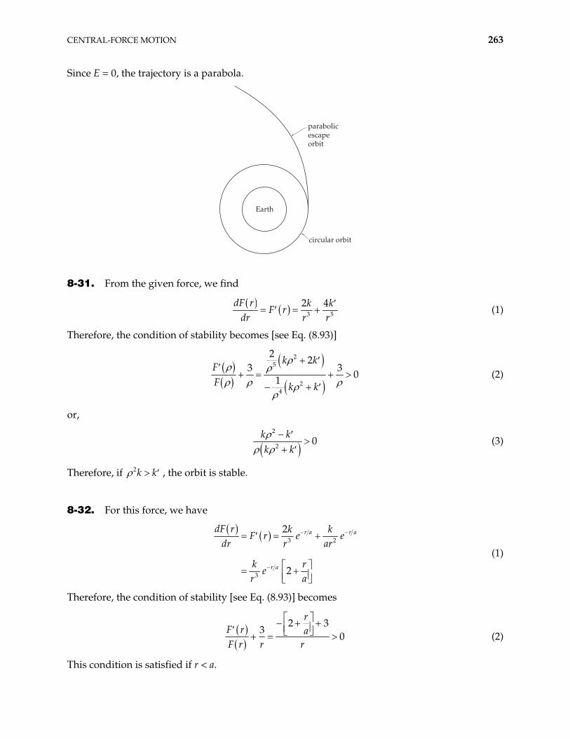
CENTRAL-FORCE MOTION 263
Since E = 0, the trajectory is a parabola.
parabolicescapeorbit
circular orbit
Earth
8-31. From the given force, we find
3
2 4dF r k kF r
dr r r5 (1)
Therefore, the condition of stability becomes [see Eq. (8.93)]
25
24
2 23
01
k kFF k k
3 (2)
or,
2
20
k kk k
(3)
Therefore, if , the orbit is stable. 2k k
8-32. For this force, we have
3 2
3
2
2
r a r a
r a
dF r k kF r e e
dr r ar
k re
r a
(1)
Therefore, the condition of stability [see Eq. (8.93)] becomes
2 3
30
rF r aF r r r
(2)
This condition is satisfied if r < a.
264 CHAPTER 8
8-33. The Lagrangian of the particle subject to a gravitational force is written in terms of the cylindrical coordinates as
2 2 2 212
L T U m r r z mgz (1)
From the constraint , we have 2 4r az
2rr
za
(2)
Therefore, (1) becomes
2
2 2 22
11
2 4 4mgr
L m r r ra a
2 (3)
Lagrange’s equation for is
2 0L d L d
mrdt dt
(4)
This equation shows that the angular momentum of the system is constant (as expected):
(5) 2 const.mr
Lagrange’s equation for r is
2
2 22 1
4 2 4mgL d L m d r
rr mr r m rr dt r a a dt a2 0 (6)
from which
2
2 2 22 21
4 2 4 2mgm r
rr mr r m r rra a a a2 0
m (7)
After rearranging, this equation becomes
2 2
22 2 3
11
4 4 2mgr m
rr ra a a m r
0m r (8)
For a circular orbit, we must have 0r r or, r = = constant. Then,
2
32mg
a m (9)
or,
2
2
2m g
a4 (10)
Equating this with 2 2 4m 2 , we have
2
2 4 2 4
2m g
ma
(11)
CENTRAL-FORCE MOTION 265
or,
2
2ga
(12)
Applying a perturbation to the circular orbit, we can write
where 1x
r x (13)
This causes the following changes:
2 2
3 3
2
1 31
r x
x
r
r x
r x
(14)
from which, we have
2 2
2 2 2
0, in lowest order
2 , in lowest ord
rr x x
r r x x x er (15)
Thus, (8) becomes
2
22 3
11
4 2mg x
xa a m
1 3 0m x (16)
But
2
32mg
a m (17)
so that (16) becomes
2 2
2
31
4 2mg
m x x xa a m 4 0 (18)
Substituting (17) into (18), we find
2
2
21
4mg
m x xa a
0 (19)
or,
2
20
4
gx x
aa
(20)
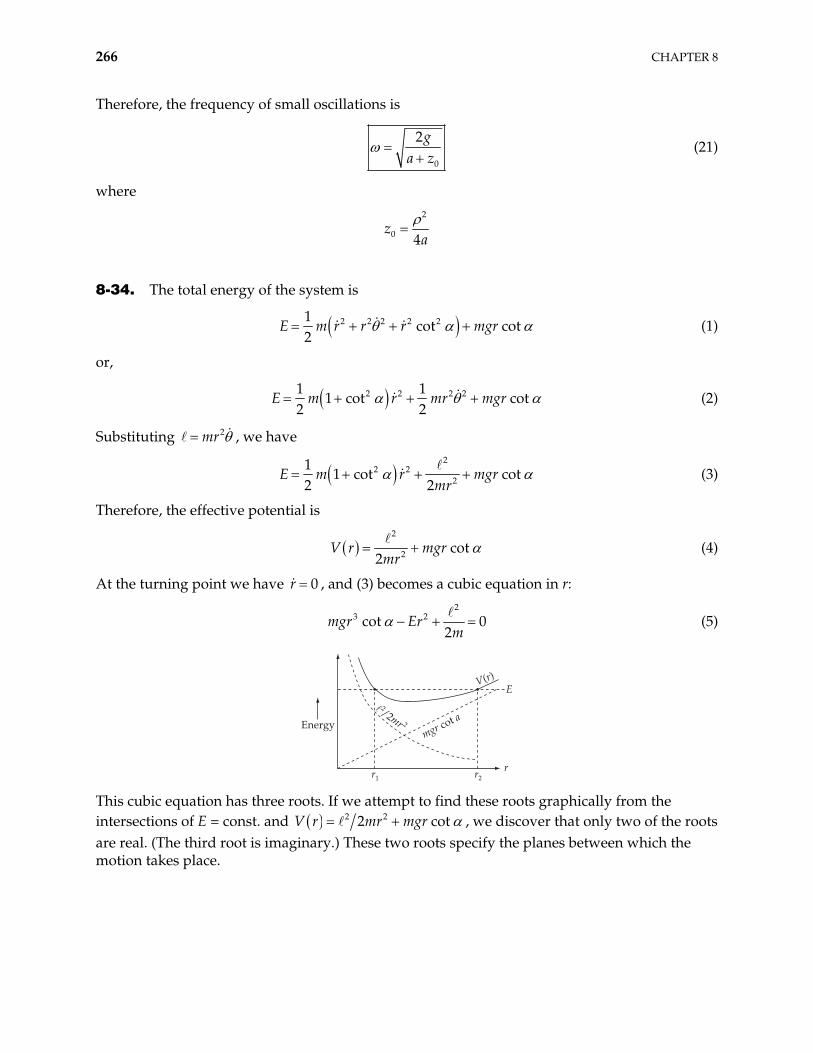
266 CHAPTER 8
Therefore, the frequency of small oscillations is
0
2ga z
(21)
where
2
0 4z
a
8-34. The total energy of the system is
2 2 2 2 21cot cot
2r r r mgrE m (1)
or,
2 2 2 21 11 cot cot
2 2r mr mgrE m (2)
Substituting 2mr , we have
2
2 22
11 cot cot
2 2r mgr
mrE m (3)
Therefore, the effective potential is
2
2 cot2
V r mgrmr
(4)
At the turning point we have , and (3) becomes a cubic equation in r: 0r
2
3 2cot 02
mgr Erm
(5)
Energymgr cot a
r2r1
E
r
V(r)
This cubic equation has three roots. If we attempt to find these roots graphically from the intersections of E = const. and 2 22 cmr mgr otV r , we discover that only two of the roots are real. (The third root is imaginary.) These two roots specify the planes between which the motion takes place.
CENTRAL-FORCE MOTION 267
8-35. If we write the radial distance r as
, cor x nst. (1)
then x obeys the oscillatory equation [see Eqs. (8.88) and (8.89)]
20 0x x (2)
where
0
3gg (3)
The time required for the radius vector to go from any maximum value to the succeeding minimum value is
0
2t (4)
where 00
2, the period of x. Thus,
0
t (5)
The angle through which the particle moves during this time interval is
0
t (6)
where is the angular velocity of the orbital motion which we approximate by a circular motion. Now, under the force F r g r , satisfies the equation
2 F r g (7)
Substituting (3) and (7) into (6), we find for the apsidal angle
0 3
3
g
g gg
g
(8)
Using 1n
kg r
r, we have
g ng
(9)
Therefore, (8) becomes
3 n (10)
268 CHAPTER 8
In order to have the closed orbits, the apsidal angle must be a rational fraction of 2 . Thus, n must be
2, 1, 6,n
n = 2 corresponds to the inverse-square-force and n = –1 corresponds to the harmonic oscillator force.
8-36. The radius of a circular orbit in a force field described by
2r ak
F r er
(1)
is determined by equating F(r) to the centrifugal force:
2
2ak
er m 3 (2)
Hence, the radius of the circular orbit must satisfy the relation
2
aemk
(3)
Since the orbit in which we are interested is almost circular, we write
1r (4)
where 1 for all values of . (With this description, the apsides correspond to the maximum and minimum values of .)
We can express the following quantities in terms of by using (4):
1 1
1ur
(5a)
2 2
2
1 1d dd r d 2 (5b)
12
221
1
au
a
F u ku e
k ea (5c)
Then, substitution into Eq. (8.20) yields
2
2 2
1 11 1
ad mkep a
d (6)
Multiplying by , using (3) and simplifying, (6) reduces to
2
2 1d
ad
0 (7)
CENTRAL-FORCE MOTION 269
This equation obviously has two types of solution depending on whether a is larger than or smaller than 1; we consider only < a. (In fact, there is no stable circular orbit for > a.)
For the initial condition, we choose 0 to be a maximum (i.e., an apside) at = 0. Then, we have
1 2
0 cos 1 , for a a (8)
This solution describes an orbit with well-defined apsides. The advance of the apsides can be found from (8) by computing for what value of is again a maximum. Thus,
2
1 a (9)
The advance of the apside is given by
1 2
2 2 1 1 a (10)
In the particular case in which a we obtain, by extending (10),
2 2 12a
(11)
so that
a
(12)
8-37. From the equations in Section 8.8 regarding Hohmann transfers:
1 2v v v
1 21 2t tv v v v v
2
1 1 2 1 2 2 1 2
2 rk k k kv
mr r r mr mr mr r r12 r
(1)
Substituting
11 2 2 24
1
2
6
6.67 10 Nm /kg 5.98 10 kg
initial height above center of Earth 2
final height above center of Earth 3
radius of the Earth 6.37 10 m
e
e
e
e
kGM
m
r r
r r
r
gives
1020 m/sv
270 CHAPTER 8
8-38. Substitute the following into Eq. (1) of problem 8-37:
11 2 2 30
111
112
6.67 10 Nm /kg 1.99 10 kg
mean Earth-sun distance 1.50 10 m
mean Venus-sun distance 1.08 10 m
sk
GMm
r
r
The result is . The answer is negative because 5275 m/sv 2r r1 ; so the rocket must be fired in the direction opposite to the motion (the satellite must be slowed down).
5275 m/s; opposite to direction of motion.v
From Eq. (8.58), the time is given by
3 2
3 2 1 2
2tr rm m
T ak k
(1)
Substituting gives
148 days
8-39. We must calculate the quantity 1v for transfers to Venus and Mars. From Eqs. (8.54), (8.53), and (8.51):
11 1
2
1 1 2 1
2
tv v v
rk kmr r r mr
where
11 3 2 30
91
92
6.67 10 m /s -kg 1.99 10 kg
mean Earth-sun distance 150 10 m
Venus 108mean sun distance 10 mMars 228
sk
GMm
r
r
Substituting gives
Venus
Mars
2.53 km/sec
2.92 km/sec
v
v
where the negative sign for Venus means the velocity kick is opposite to the Earth’s orbital motion.
Th us, a Mars flyby requires a larger than a Venus flyby.v
CENTRAL-FORCE MOTION 271
8-40. To crash into the sun, we calculate 1v from Eq. (8.54) with r = mean distance from sun to Earth, and = radius of the sun. Using Eqs. (8.54), (8.53), and (8.51) we have
1
2r
21 sun
1 1 2 1
2 s sGM GMrv
r r r r
Substituting
11 2 2
30
111
82 sun
6.67 10 Nm /kg
1.99 10 kg
1.5 10 m
6.96 10 m
s
se
G
M
r r
r r
gives
1 sun26.9 km/secv
To escape from the solar system, we must overcome the gravitational pull of both the sun and Earth. From conservation of energy ( final 0E ) we have:
210
2s e
se e
GM m GM mmv
r r
Substituting values gives
43500 m/sv
Now
escape
43500 29700 m/s
13.8 km/s
i
s
se
v v v
GMv
r
v
To les
send the waste out of the solar system requiress energy than crashing it into the sun.
8-41. From the equations in Section 8.8 regarding Hohmann transfers
1 2
1 2
1 2t t
v v v
v v v v
where
272 CHAPTER 8
1
21
1 1 2 1
2;t
rk kv v
mr r r mr
2
11
2 1 2 2
2;t
rk kv v
mr r r mr
Substituting
11 2 2 24
6 51
82
6.67 10 Nm /kg 5.98 10 kg
200 km 6.37 10 m 2 10 m
mean Earth-moon distance 3.84 10 m
e
e
kGM
m
r
r r
gives
3966 m/sv
From Eq. (8.58), the time of transfer is given by
3 2
3 2 1 2
2tr rm m
T ak k
Substituting gives
429,000 sec. 5 days
8-42.
r
11 2 2
24
5 61
2
83
6.67 10 Nm /kg
5.98 10 kg
2 10 m 6.37 10 m
?
mean Earth-moon distance 3.84 10 m
e
G
M
r
r
We can get from Kepler’s Third Law (with = 1 day) 2r
1 32
72 2 4.225 10 m
4eGM
r
We know 2E GMm r
CENTRAL-FORCE MOTION 273
So
111
1
102
93
3.04 10 J2
4.72 10 J
5.19 10 J
eGM mE r
r
E r
E r
To place the satellite in a synchronous orbit would require a minimum energy of 2 1E r E r
112.57 10 J
8-43. In a circular orbit, the velocity v of satellite is given by 0
20
02
mv GMm GMv
R R R
where M is the Earth’s mass.
Conservation of energy implies
2 21 2
2 2mv mvGMm GMm
R R2
Conservation of angular momentum gives
1 22mRv m Rv
From these equations, we find
143GM
vR
so the velocity need to be increased by a factor 4 3 to change the orbit.
8-44. The bound motion means that 2
02
mvE V
where r akr
V e .
The orbit of particle moving in this central force potential is given by
274 CHAPTER 8
min
min
2
2
2
2 2
2
/
22
12
2
r
r
r
rar
r drr
E Vr
drr keE
r r
In first order of , this is ( / )r a
( ) 2 22 2
2 2
2 22 2
rdr dr
k k k kr E r E
r r a a r r
Now effectively, this is the orbit of particle of total energy k
Ea
moving in potential kr
. It is
well known that this orbit is given by (see Chapter 8)
1 cosr
where2
k and
2
2
21
kE
k a
If 0 1 , the orbit is ellipsoid; if 0 , the orbit is circular.
8-45.
a) In equilibrium, for a circular orbit of radius r0,
2 00 0
0
FF m r
mr
b) The angular momentum (which is conserved) of a particle in circular orbit is
20L mr 3
0mFr
The force acting on a particle, which is placed a distance r (r is very close to equilibrium position ) from the center of force is or
32
0 03
3 2 2
0 0 0 03 2 40 0 0
3 3
LF m r F F
mr
L L Lr r F r r k r r
mr mr mr
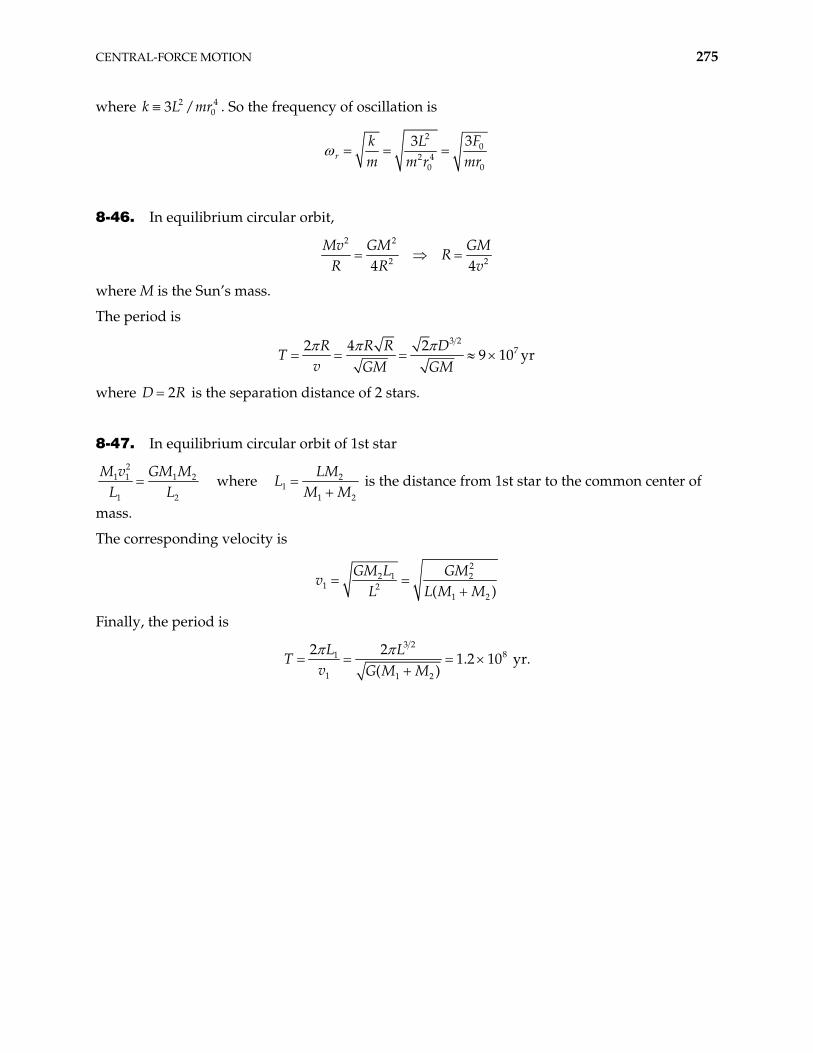
CENTRAL-FORCE MOTION 275
where . So the frequency of oscillation is 203 /k L mr4
2
02 4
0 0
33r
Fk Lm m r mr
8-46. In equilibrium circular orbit,
2 2
2 24 4Mv GM GM
RR R v
where M is the Sun’s mass.
The period is
3 2
72 4 29 10 yr
R R R Dv GM GM
T
where D is the separation distance of 2 stars. 2R
8-47. In equilibrium circular orbit of 1st star 2
1 1 1 2
1 2
M v GM ML L
where 21
1 2
LML
M M is the distance from 1st star to the common center of
mass.
The corresponding velocity is
2
2 1 21 2
1 2( )GM L GM
vL L M M
Finally, the period is
3 2
81
1 1 2
2 21.2 10 yr.
( )L L
v G M MT

276 CHAPTER 8
CHAPTER 9 Dynamics of a
System of Particles
9-1. Put the shell in the z > 0 region, with the base in the x-y plane. By symmetry, 0x y .
2
1
2
1
2 2 2
0 02 2 2
0 0
sin
sin
r
r rr
r r
zr dr d dz
r dr d d
Using z = r cos and doing the integrals gives
4 4
2 1
3 32 1
3
8
r rz
r r
9-2.
z
h
x
ya
zha
h= ! +"
By symmetry, 0x y .
Use cylindrical coordinates , , z.
0 mass density
277
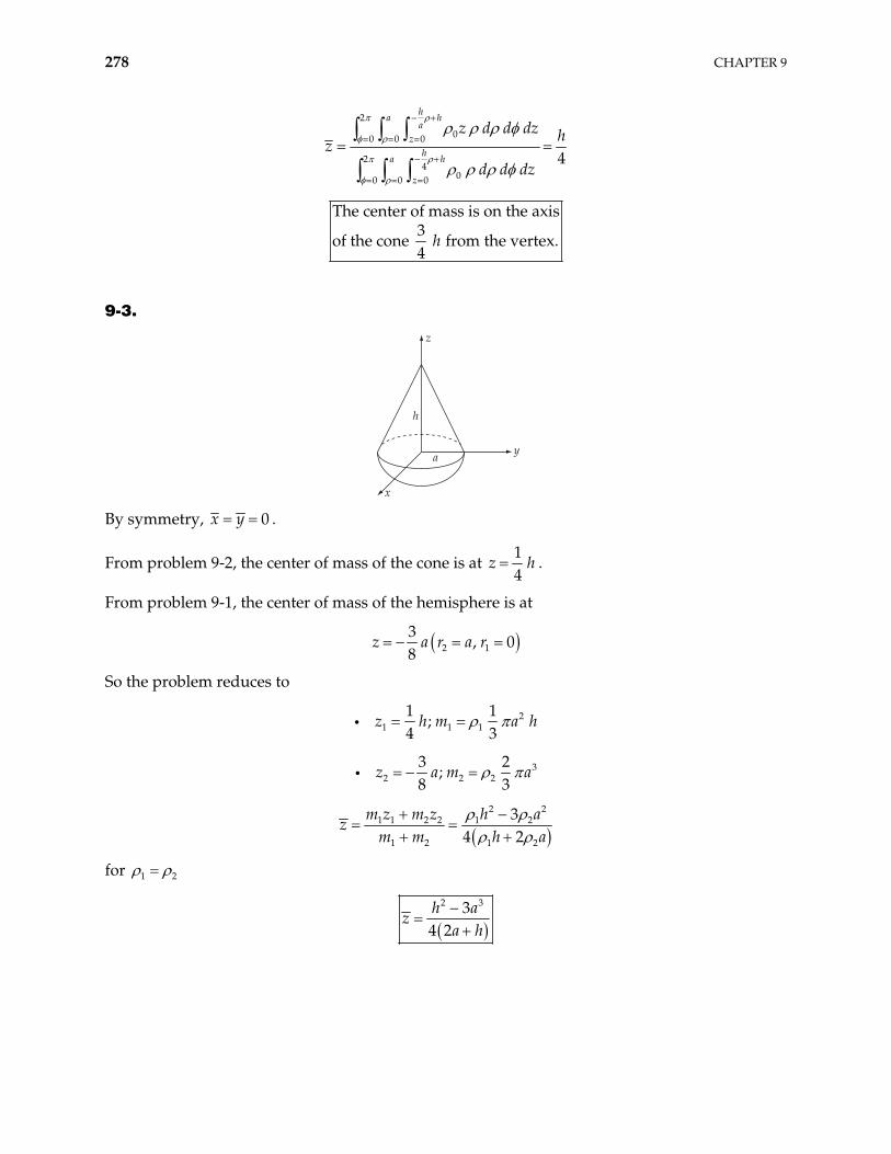
278 CHAPTER 9
2
00 0 0
24
00 0 0
4
ha h
az
ha h
z
z d d dz hz
d d dz
The center of mass is on the axis
3of the cone from the vertex.
4h
9-3.
z
h
x
ya
By symmetry, 0x y .
From problem 9-2, the center of mass of the cone is at 14
z h .
From problem 9-1, the center of mass of the hemisphere is at
2 13
, 08
z a r a r
So the problem reduces to
21 1 1
1 1;
4 3z h m a h
32 2 2
3 2;
8 3z a m a
2 2
1 1 2 2 1 2
1 2 1 2
34 2
m z m z h az
m m h a
for 1 2
2 33
4 2h a
za h
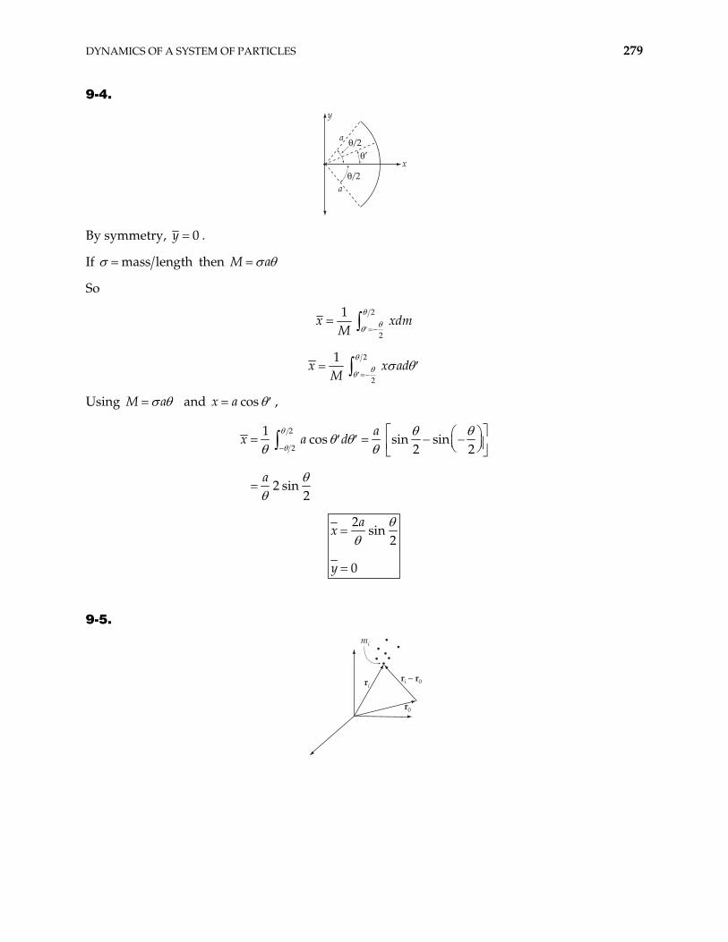
DYNAMICS OF A SYSTEM OF PARTICLES 279
9-4.
#$
#/2
#/2
y
x
a
a
By symmetry, 0y .
If mass length then M a
So
2
2
1x xdm
M
2
2
1x x
Mad
Using M a and cosx a ,
2
2
1cos sin sin
2 2
2 sin2
ax a d
a
2sin
2
0
ax
y
9-5.
ri – r0
r0
ri
mi
280 CHAPTER 9
th
th1
position of the particle
mass of the particle
total mass
constant gravitational field
i
i
i
m i
M m
r
g
Calculate the torque about 0r
0
0
1 0
0
0
i
i i
i i
i i
i i i
i i
m
m m
m m
m M
r r F
r r g
r g r g
r g r
r g r g
g
Now if the total torque is zero, we must have
0i im Mr r
or
01
i imM
r r
which is the definition of the center of mass. So
0 CM0 about or center of gravity center of mass.
r r
9-6. Since particle 1 has F = 0, , then 0 0 0r v 1 0r . For particle 2
02 0 ˆ ˆthen
FF r
mF x x
Integrating twice with gives 0 0 0r v
202 ˆ
2F
r tm
x
201 1 2 2CM
1 2
ˆ4Fm m
tm m mr r
r x
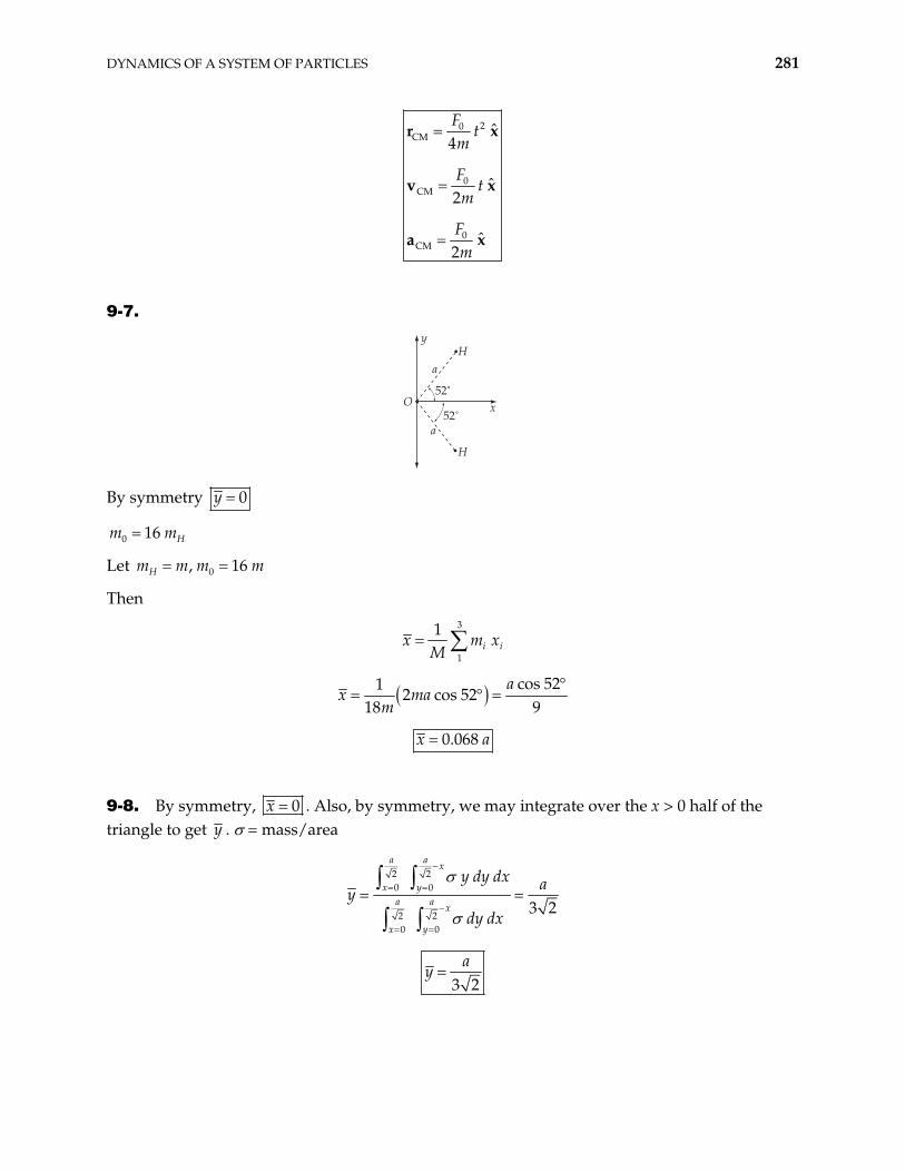
DYNAMICS OF A SYSTEM OF PARTICLES 281
20CM
0CM
0CM
ˆ4
ˆ2
ˆ2
Ft
m
Ft
m
Fm
r x
v x
a x
9-7.
O
y
a
a
H
H
x52˚
52˚
By symmetry 0y
0 16 Hm m
Let 0, 16Hm m m m
Then
3
1
1i ix m
Mx
cos 521
2 cos 5218 9
ax ma
m
0.068x a
9-8. By symmetry, 0x . Also, by symmetry, we may integrate over the x > 0 half of the triangle to get y . = mass/area
2 20 0
2 20 0
3 2
a ax
x ya a
x
x y
y dy dx ay
dy dx
3 2
ay
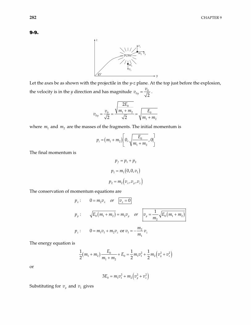
282 CHAPTER 9
9-9.
POW!
45˚
z
y
m1
m2
v1
vy
vz
Let the axes be as shown with the projectile in the y-z plane. At the top just before the explosion,
the velocity is in the y direction and has magnitude 00 2y
vv .
0
1 20 00
1 2
2
2 2y
Em mv E
vm m
where and are the masses of the fragments. The initial momentum is 1m 2m
01 2
1 2
0, , 0iE
p m mm m
The final momentum is
1 2fp p p
1 1 10,0,p m v
2 2 , ,x y zp m v v v
The conservation of momentum equations are
2: 0x xv or v 0xp m
0 1 2 2 0 1 22
1:y y yp E m m m v or v E m m
m
21 1 2 1
1
or : 0z z zm
p m v m v v vm
The energy equation is
2 201 2 0 1 1 2
1 2
12 2 2
21 1y z
Em m E m v m v v
m m
or
2 20 1 1 23 2
y zE m v m v v
Substituting for yv and v gives 1
DYNAMICS OF A SYSTEM OF PARTICLES 283
0 1 2 122 1 2
2z
E m m mv
m m m
21
1z
mv v
m gives
0 2 11
1 1 2
2E m mv
m m m
So
travels straight down with speed =1m 1v
travels in the y-z plane 2m
1 2 0 1 22 22
2 1 2
1 2 11 1
1 2
4
2tan tan
y z
z
y
E m mv v v
m m m
m m mvv m m
The mass is the largest it can be when 1m 1 0v , meaning 22m m1 and the mass ratio is
1
2
12
mm
9-10.
x2x1
x
yB
A#
First, we find the time required to go from A to B by examining the motion. The equation for the y-component of velocity is
0 sinyv v gt (1)
At B, v ; thus 0y 0 sinBt v g . The shell explodes giving m and horizontal velocities v and (in the original direction). We solve for and using conservation of momentum and energy.
1 2m 1
2v 1v 2v
1 2 0 1 1 2osx 2: cp m m v m v m v (2)
2 2 21 2 0 1 1 2
1 1: cos
2 2m v E m v 2
212
m vE m (3)
Solving for in (2) and substituting into (3) gives an equation quadratic in v . The solution is 2v 1
284 CHAPTER 9
21 0
1 1 2
cosm E
v vm m m
(4)
and therefore we also must have
12 0
2 1 2
cosm E
v vm m m
(5)
Now we need the positions where m and m land. The time to fall to the ocean is the same as the time it took to go from A to B. Calling the location where the shell explodes x = 0 gives for the positions of and upon landing:
1 2
1m 2m
1 1 2 2;Bx v t x v tB (6)
Thus
01 2 1 2
sinvx x v v
g (7)
Using (4) and (5) and simplifying gives
0 11 2
1 2 2 1
sin 2v m mEg m m m m
2x x (8)
9-11. The term in question is
b
f
For n = 3, this becomes
12 13 21 23 31 32 12 21 13 31 23 32f f f f f f f f f ff f
But by Eq. (9.1), each quantity in parentheses is zero. Thus
3 3
1 1
0f
9-12.
a) 00 ln
mv v u
m
Assuming , we have 0 0v
m 10
100 lns 9
v08
2.02 m/s; yes, he runs out of gas.v
DYNAMICS OF A SYSTEM OF PARTICLES 285
b) Relative to Stumblebum’s original frame of reference we have:
Before throwing tank
98 kg
2.02 m/s
After throwing the tank we want Stumblebum’s velocity to be slightly greater than 3 m/s (so that he will catch up to the orbiter).
8 kg 90 kg
3m/sV
Conservation of momentum gives
98 kg 2.02 m/s 90 kg 3 m/s 8 kg
9 m/s
v
v
(This velocity is relative to Stumblebum’s original reference frame; i.e., before he fires his pressurized tank.) Since Stumblebum is traveling towards the orbiter at 2.02 m/s, he must throw the tank at v = 9 m/s + 2.02 m/s
11 m/sv
9-13. From Eq. (9.9), the total force is given by
( )eF f
As shown in Section 9.3, the second term is zero. So the total force is
( )eF
It is given that this quantity is zero.
Now consider two coordinate systems with origins at 0 and 0
O
O$
m%
r%$r%
r0
where
is a vector from 0 to 0 0r
r is the position vector of m in 0
286 CHAPTER 9
r is the position vector of m in 0
We see that 0ar r r
The torque in 0 is given by
( )er F
The torque in 0 is
( )
( )0
( ) ( )0
( )0
e
e
e e
e
r F
r r F
r F r F
r F
But it is given that ( ) 0eF
Thus
9-14. Neither Eq. (9.11) or Eq. (9.31) is valid for a system of particles interacting by magnetic forces. The derivations leading to both of these equations assumes the weak statement of Newton’s Third Law [Eq. (9.31) assumes the strong statement of the Third Law also], which is
f f
That this is not valid for a system with magnetic interactions can be seen by considering two particles of charge and moving with velocities and : 1q 2q 1v 2v
q1q2
v2
f21
v1f12
Now
ij i i ijqf v B
where ijB is the magnetic field at due to the motion of iq jq .
DYNAMICS OF A SYSTEM OF PARTICLES 287
Since ijf is perpendicular to both and iv ijB (which is either in or out of the paper), ijf can only be parallel to jif if and iv jv are parallel, which is not true in general.
Thus, equations (9.11) and (9.31) are not valid for
ystem of particles with magnetic interactions.a s
9-15. = mass/length
dp
Fdt
becomes
mg mv mv
where m is the mass of length x of the rope. So
;m x m x
2
2
dvx g x x v
dt
dv dxx g x v
dx dt
dvx g xv v
dx
Try a power law solution:
1;n ndvv ax nax
dx
Substituting,
1 2 2n nx g x ax nax a x n
or
2 21 nx g a n x
Since this must be true for all x, the exponent and coefficient of x must be the same on both sides of the equation.
Thus we have: 1 = 2n or 12
n
2 21 or
3g
g a n a
So
2
3gx
v
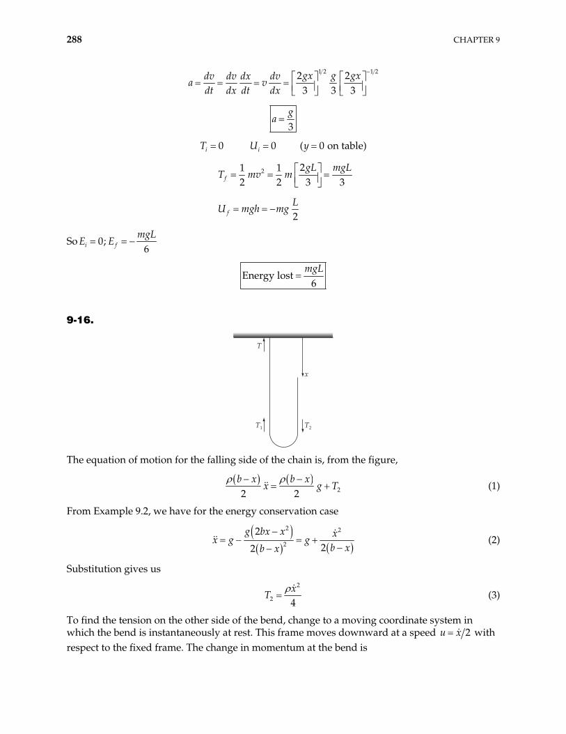
288 CHAPTER 9
1 2 1 22 2
3 3 3gx g gxdv dv dx dv
dt dx dt dxa v
3g
a
T U 0 0 ( 0 on ti i y able)
2 21 12 2 3f
gL mgLT mv m
3
2fL
U mgh mg
So 0;6i f
mgLE E
Energy lost6
mgL
9-16.
T1 T2
T
x
The equation of motion for the falling side of the chain is, from the figure,
22 2b x b x
x g T (1)
From Example 9.2, we have for the energy conservation case
2 2
2
2
22
g bx x xx g g
b xb x (2)
Substitution gives us
2
2 4x
T (3)
To find the tension on the other side of the bend, change to a moving coordinate system in which the bend is instantaneously at rest. This frame moves downward at a speed 2u x with respect to the fixed frame. The change in momentum at the bend is
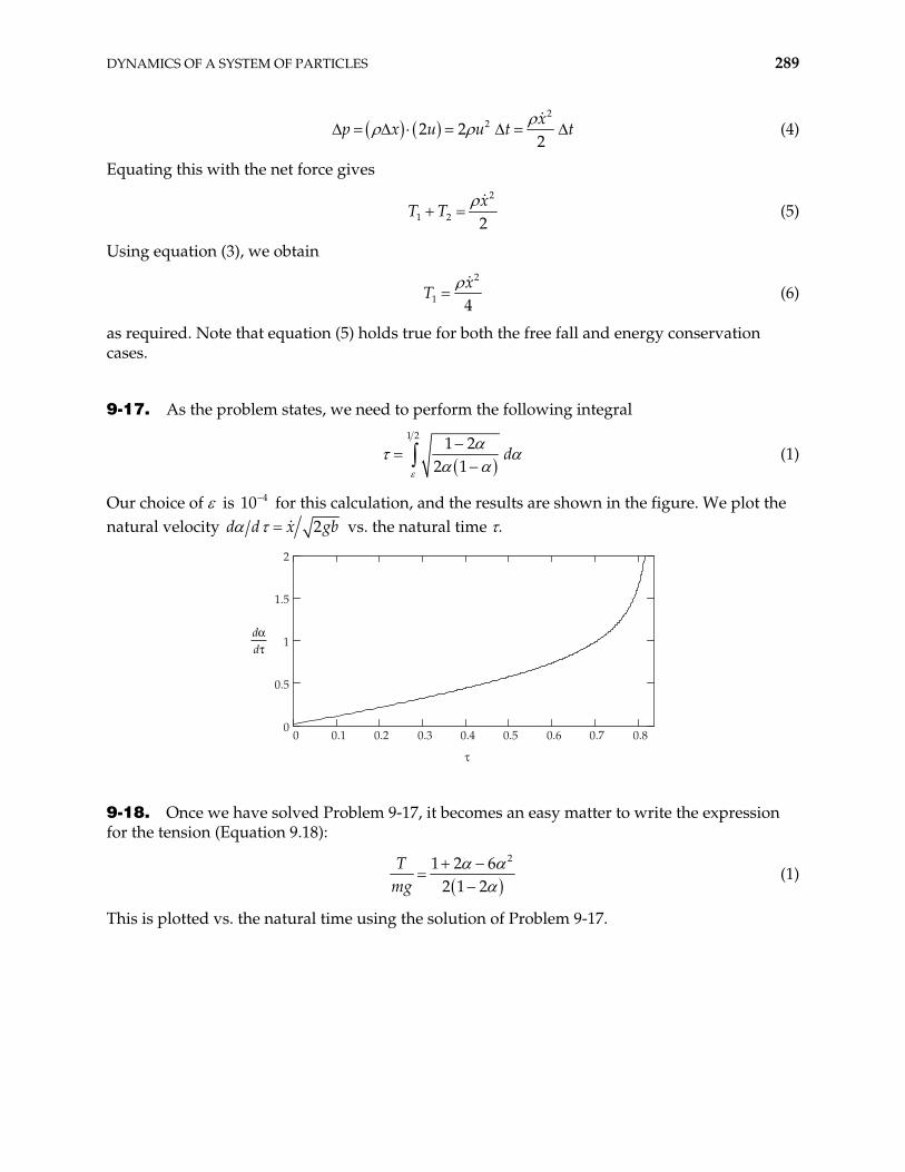
DYNAMICS OF A SYSTEM OF PARTICLES 289
2
22 22x
p x u u t t (4)
Equating this with the net force gives
2
1 2 2x
T T (5)
Using equation (3), we obtain
2
1 4x
T (6)
as required. Note that equation (5) holds true for both the free fall and energy conservation cases.
9-17. As the problem states, we need to perform the following integral
1 2 1 2
2 1d (1)
Our choice of is 10 for this calculation, and the results are shown in the figure. We plot the natural velocity
4
2d d x gb vs. the natural time .
0 0.1 0.2 0.3 0.4 0.5 0.6 0.7 0.80
0.5
1
1.5
2
&
dd%&
9-18. Once we have solved Problem 9-17, it becomes an easy matter to write the expression for the tension (Equation 9.18):
21 2 6
2 1 2T
mg (1)
This is plotted vs. the natural time using the solution of Problem 9-17.
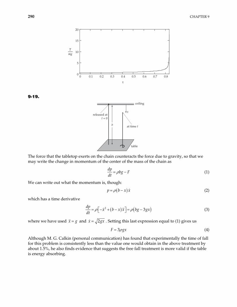
290 CHAPTER 9
0 0.1 0.2 0.3 0.4 0.5 0.6 0.7 0.80
5
10
15
20
&
Tmg
9-19.
released att = 0
x
at time t
ceiling
table
b
The force that the tabletop exerts on the chain counteracts the force due to gravity, so that we may write the change in momentum of the center of the mass of the chain as
dp
bg Fdt
(1)
We can write out what the momentum is, though:
p b x x (2)
which has a time derivative
2 3dp
x b x x bg gxdt
(3)
where we have used and x g 2x gx
3
. Setting this last expression equal to (1) gives us
F gx (4)
Although M. G. Calkin (personal communication) has found that experimentally the time of fall for this problem is consistently less than the value one would obtain in the above treatment by about 1.5%, he also finds evidence that suggests the free fall treatment is more valid if the table is energy absorbing.
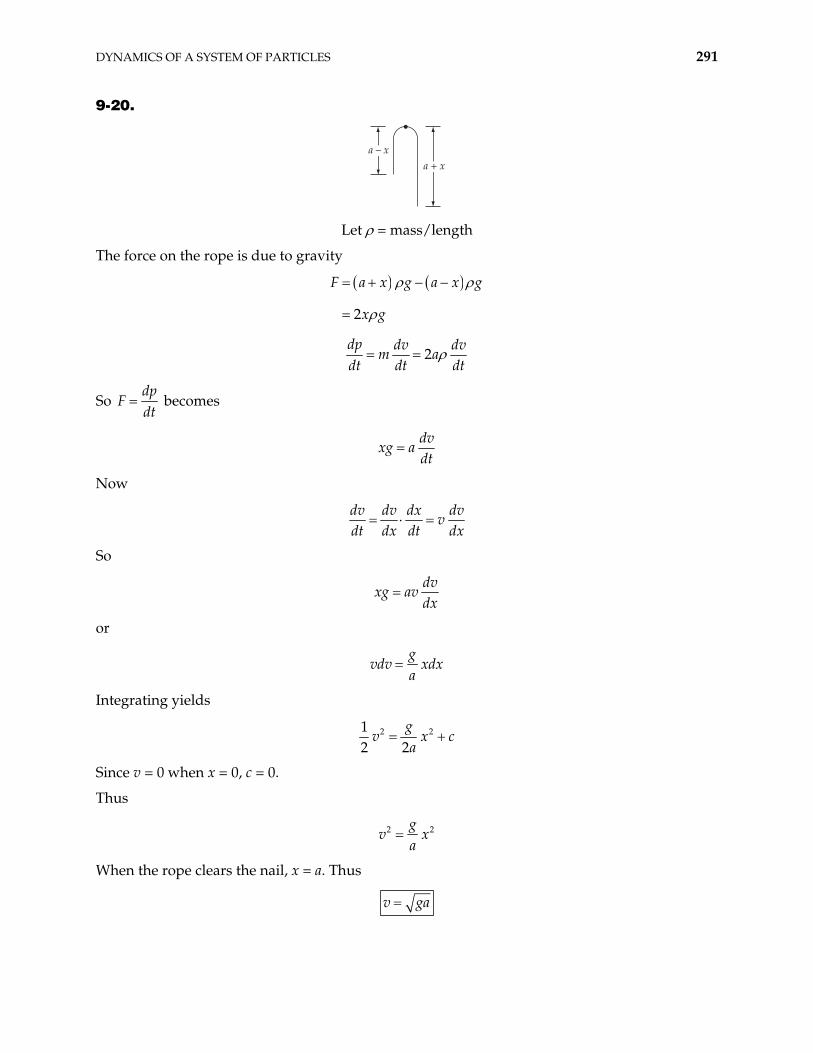
DYNAMICS OF A SYSTEM OF PARTICLES 291
9-20.
a – xa + x
Let = mass/length
The force on the rope is due to gravity
2
F a x g a x g
x g
2dp dv dv
m adt dt dt
So dp
Fdt
becomes
dv
xg adt
Now
dv dv dx dv
vdt dx dt dx
So
dv
xg avdx
or
g
vdv xdxa
Integrating yields
2 212 2
gv x
ac
Since v = 0 when x = 0, c = 0.
Thus
2 2gv x
a
When the rope clears the nail, x = a. Thus
v ga
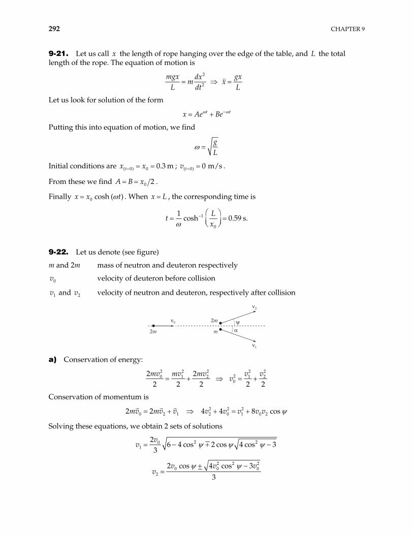
292 CHAPTER 9
9-21. Let us call the length of rope hanging over the edge of the table, and the total length of the rope. The equation of motion is
x L
2
2
mgx gxdxm x
L dt L
Let us look for solution of the form
t tx Ae Be
Putting this into equation of motion, we find
gL
Initial conditions are ; ( 0) 0 0.3 mtx x ( 0) 0 m/stv .
From these we find 0 2A B x .
Finally 0 cosh ( )x x t . When , the corresponding time is x L
1
0
1cosh 0.59 s.
Lt
x
9-22. Let us denote (see figure)
m and 2m mass of neutron and deuteron respectively
0v velocity of deuteron before collision
1v and v velocity of neutron and deuteron, respectively after collision 2
2m
2m'0
'2
'1
m %(
a) Conservation of energy:
2 2 2 2
20 1 2 10
22 2 2 2
mv mv mv v vv
22
22
Conservation of momentum is
2 2 2 2 20 2 1 2 0 1 0 24 4 8 cosmv mv v v v v v v
Solving these equations, we obtain 2 sets of solutions
2 201
26 4 cos 2 cos 4 cos 3
3v
v
2 2
0 02
2 cos 4 cos 33
v vv
20v
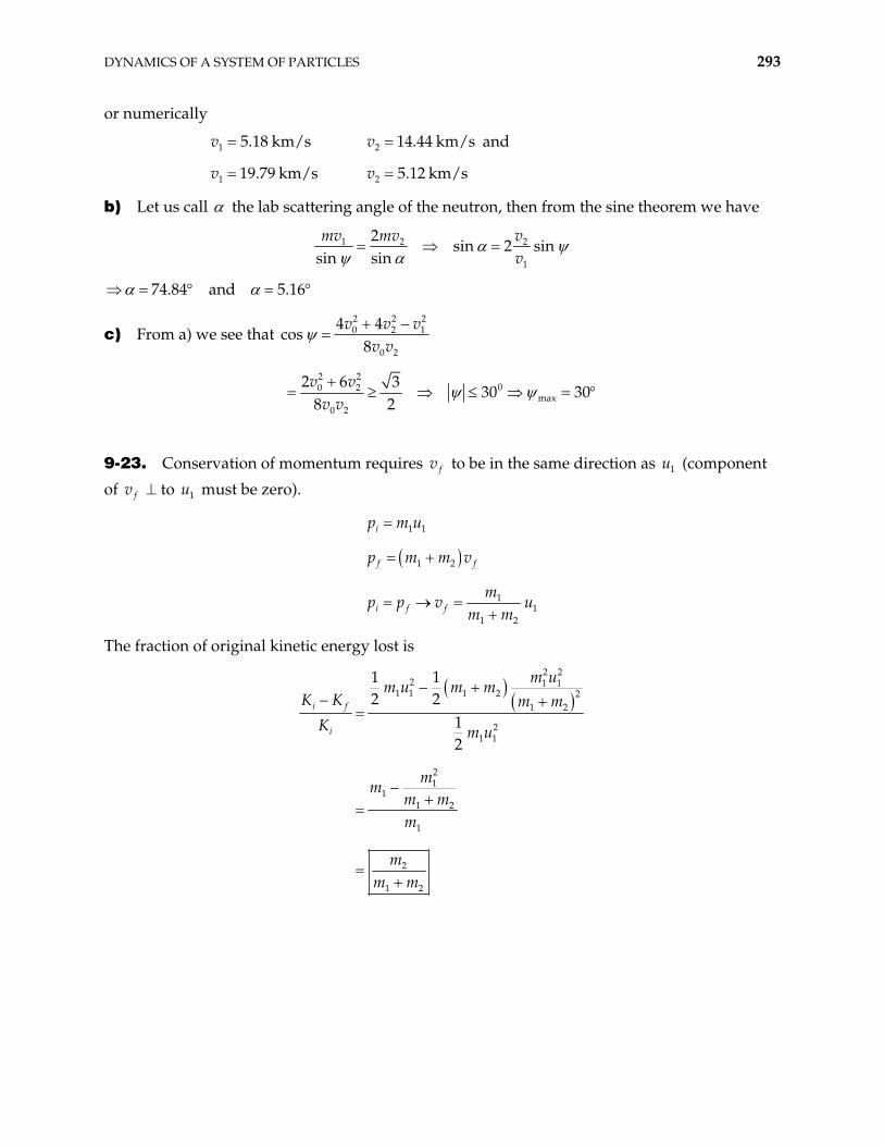
DYNAMICS OF A SYSTEM OF PARTICLES 293
or numerically
1 5.18 km/sv 2 14.44 km/sv and
1 19.79 km/sv 2 5.12 km/sv
b) Let us call the lab scattering angle of the neutron, then from the sine theorem we have
1 2 2
1
2sin 2 sin
sin sinmv mv v
v
74.84 and 5.16
c) From a) we see that 2 20 2
0 2
4 4cos
8v v v
v v
21
2 2
00 2max
0 2
2 6 330 30
8 2v v
v v
9-23. Conservation of momentum requires fv to be in the same direction as u (component
of 1
fv to must be zero). 1u
1 1ip m u
1 2f fp m m v
11
1 2i f f
mp p v
m mu
The fraction of original kinetic energy lost is
2 22 1 1
1 1 1 2 21 2
21 1
21
11 2
1
2
1 2
1 12 2
12
i f
i
m um u m m
K K m mK m u
mm
m mm
mm m
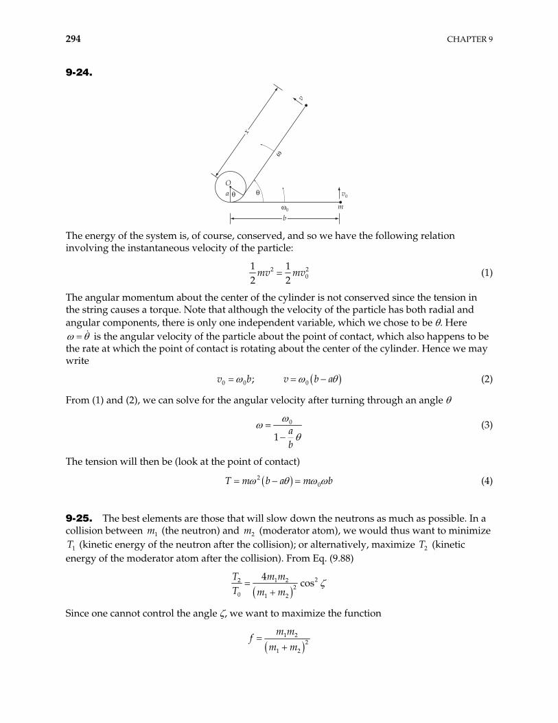
294 CHAPTER 9
9-24.
)0
b
v0
x
)
v
m
aO
# #
The energy of the system is, of course, conserved, and so we have the following relation involving the instantaneous velocity of the particle:
20
1 12 2
mv mv2 (1)
The angular momentum about the center of the cylinder is not conserved since the tension in the string causes a torque. Note that although the velocity of the particle has both radial and angular components, there is only one independent variable, which we chose to be . Here
is the angular velocity of the particle about the point of contact, which also happens to be the rate at which the point of contact is rotating about the center of the cylinder. Hence we may write
0 0 0;v b v b a (2)
From (1) and (2), we can solve for the angular velocity after turning through an angle
0
1 ab
(3)
The tension will then be (look at the point of contact)
20T m b a m b (4)
9-25. The best elements are those that will slow down the neutrons as much as possible. In a collision between (the neutron) and (moderator atom), we would thus want to minimize
(kinetic energy of the neutron after the collision); or alternatively, maximize T (kinetic energy of the moderator atom after the collision). From Eq. (9.88)
1m 2m
1T 2
22 1 22
0 1 2
4cos
T m mT m m
Since one cannot control the angle , we want to maximize the function
1 22
1 2
m mf
m m
DYNAMICS OF A SYSTEM OF PARTICLES 295
with respect to . ( m = constant) 2m 1
2 2
1 1 21 24
2 1 2
0 when m m mdf
m mdm m m
By evaluating 1 2
2
22 m m
d fdm
1 2m m
one can show that the equilibrium point is a maximum. Thus, is a
maximum for . Back to reactors, one would want elements whose mass is as close as possible to the neutron mass (thus, as light as possible). Naturally, there are many other factors to consider besides mass, but in general, the lower the mass of the moderator, the more energy is lost per collision by the neutrons.
2T
9-26. The internal torque for the system is
1 12 2 21N r f r f (1)
where f is the force acting on the first particle due to the second particle. Now 12
21 12f f (2)
Then,
1 2 12
1 2 2 1 2 10
1 2 1 20
rk
v
krv
N r r f
r r r r r r
r r r r (3)
This is not zero in general because 1 2r r and 1 2r r are not necessarily parallel. The
internal torque vanishes only if the internal force is directed along the line joining two particles. The system is not conservative.
9-27. The equation for conservation of yp in the lab system is (see fig. 9-10c):
1 1 2 20 sin sim v m v n
Thus
1 1
2 2
sin sinm vm v
or
1 1
2 2
sin sinm Tm T
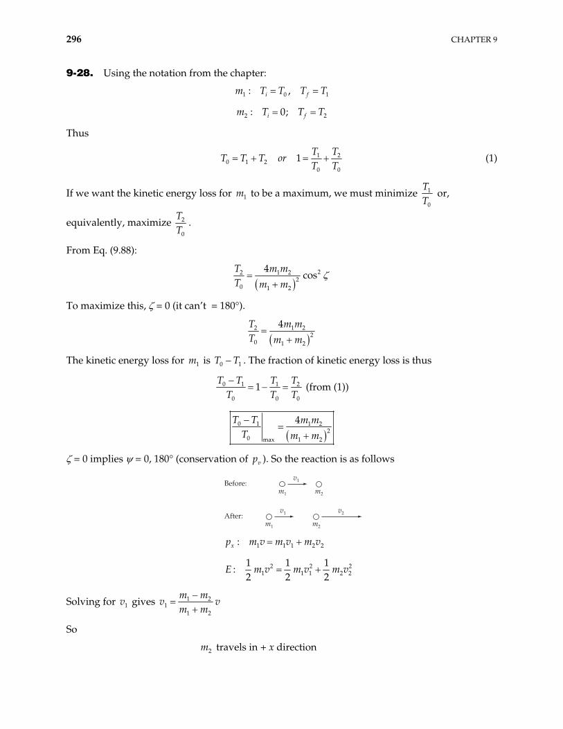
296 CHAPTER 9
9-28. Using the notation from the chapter:
1 0: ,i fm T T T T1
2 2: 0;i fm T T T
Thus
10 1 2
0 0
1T T
T T T orT T
2 (1)
If we want the kinetic energy loss for to be a maximum, we must minimize 1m 1
0
TT
or,
equivalently, maximize 2
0
TT
.
From Eq. (9.88):
22 1 22
0 1 2
4cos
T m mT m m
To maximize this, = 0 (it can’t = 180°).
2 12
0 1 2
4T m mT m m
2
1
The kinetic energy loss for is T . The fraction of kinetic energy loss is thus 1m 0 T
0 1 1
0 0
1T T T T
T T2
0T (from (1))
0 1 1 22
0 1 2max
4T T m mT m m
= 0 implies = 0, 180° (conservation of ). So the reaction is as follows vp
Before:
After:
m1
v1
m2
m1
v1
m2
v2
1 1 1 2:xp m v m v m v2
2 21 1 1
1 1 1:
2 2 2E m v m v m 2
2 2v
Solving for gives 1v 1 21
1 2
m mv v
m m
So
travels in + x direction 2m
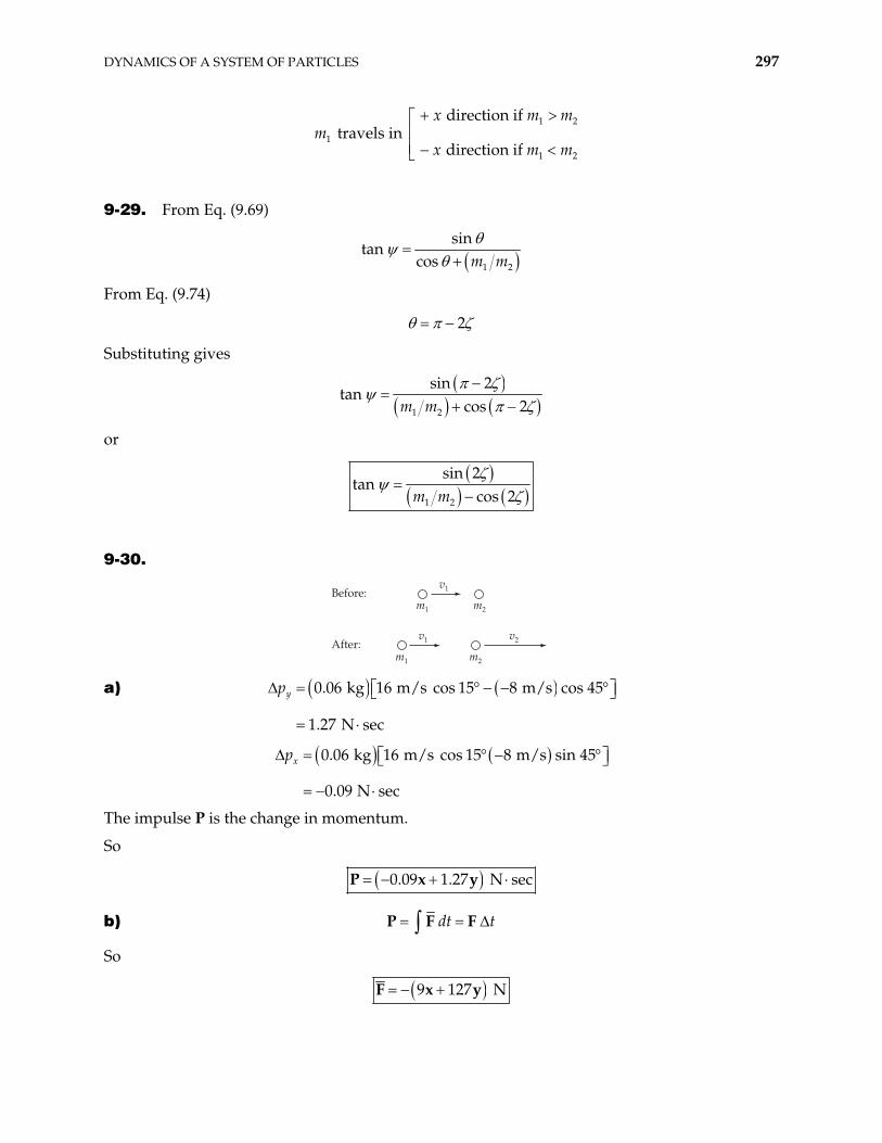
DYNAMICS OF A SYSTEM OF PARTICLES 297
m travels in 1
1 2
1 2
direction if
direction if
x m
x m
m
m
9-29. From Eq. (9.69)
1 2
sintan
cos m m
From Eq. (9.74)
2
Substituting gives
1 2
sin 2tan
cos 2m m
or
1 2
sin 2tan
cos 2m m
9-30.
Before:
After:
m1
v1
m2
m1
v1
m2
v2
a) 0.06 kg 16 m/s cos 15 8 m/s cos 45
1.27 N sec
yp
0.06 kg 16 m/s cos 15 8 m/s sin 45
0.09 N sec
xp
The impulse P is the change in momentum.
So
0.09 1.27 N secP x y
b) dt tP F F
So
9 127 NF x y
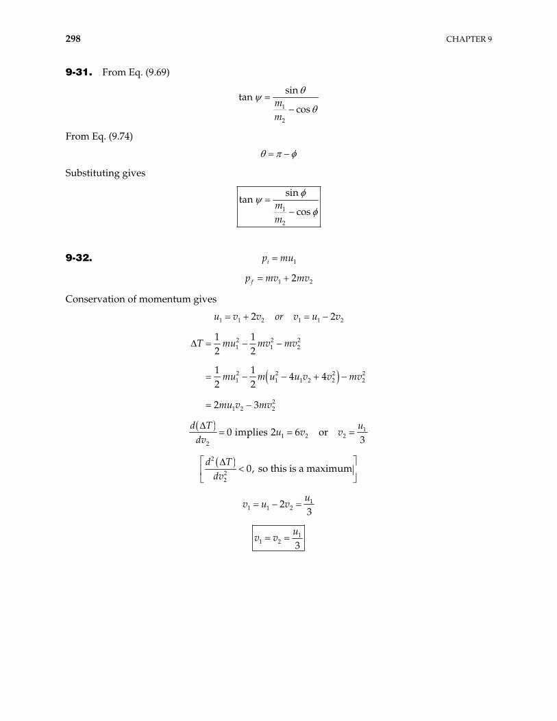
298 CHAPTER 9
9-31. From Eq. (9.69)
1
2
sintan
cosmm
From Eq. (9.74)
Substituting gives
1
2
sintan
cosmm
9-32. 1ip mu
1 22fp mv mv
Conservation of momentum gives
1 1 2 1 12 2u v v or v u v2
2 2 21 1 2
2 2 21 1 1 2 2
21 2 2
1 12 2
1 14 4
2 2
2 3
T mu mv mv
mu m u u v v mv
mu v mv
22
11 2 2
2
0 implies 2 6 or3
d T uu v v
dv
2
22
0, so this is a maximumd T
dv
11 1 22
3u
v u v
11 2 3
uv v
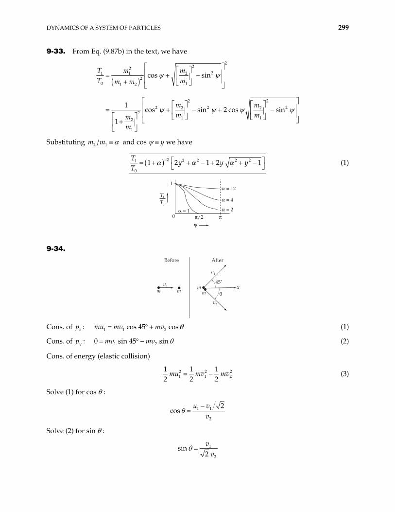
DYNAMICS OF A SYSTEM OF PARTICLES 299
9-33. From Eq. (9.87b) in the text, we have
222
21 1 22
0 11 2
2 22 22 2
21 12
1
cos sin
1cos sin 2 cos sin
1
T m mT mm m
m mm mm
m
2
Substituting 2 1m m and cos y we have
2 2 2 2 21
0
1 2 1 2T
y y yT
1 (1)
% = 12
% = 4
% = 2% = 1*/2(
*
1
0
TT
1
0
9-34.
Before After
45˚
mm
mx
m
v2
v1
u1
#
Cons. of zp : 1 1 2cos 45 cosmu mv mv (1)
Cons. of yp : 1 20 sin 45 simv mv n (2)
Cons. of energy (elastic collision)
2 21 1
1 1 12 2 2
mu mv mv22 (3)
Solve (1) for cos :
1 1
2
2cos
u vv
Solve (2) for sin :
1
2
sin2v
v
300 CHAPTER 9
Substitute into , simplify, and the result is 2 2cos sin 1
2 2 21 2 1 12u v v u v1
Combining this with (3) gives
21 12 2v u 1v
We are told v , hence 1 0
1 1 2v u
Substitute into (3) and the result is
2 1 2v u
Since v , (2) implies 1 v2
0 45
9-35. From the following two expressions for 1 0T T ,
2
1 12
0 1
Eq. (9.82)T vT u
222
21 1 22
11 2
cos sin Eq. (9.87b)m
T mm mT m
we can find the expression for the final velocity of in the lab system in terms of the scattering angle :
1v 1m
2
21 1 21
1 2 1
cos sinm u m
m m mv (1)
If time is to be constant on a certain surface that is a distance r from the point of collision, we have
1 0r v t (2)
Thus,
2
21 1 0 2
1 2 1
cos sinm u t m
m m mr (3)
This is the equation of the required surface. Let us consider the following cases:
DYNAMICS OF A SYSTEM OF PARTICLES 301
i) : 2 1m m
21 01 0cos 1 sin cos
2u t
r u t (4)
(The possibility r = 0 is uninteresting.)
iI) : 2 12m m
21 0 cos 4 sin3
u tr (5)
iII) : Rewriting (3) as 2m
2 2
1 1 02
1 2 1 2
2
cos sin1
1
m u tm m m mm
r (6)
and taking the limit , we find 2m
1 0r u t (7)
All three cases yield spherical surfaces, but with the centers displaced:
v1t0–v1t0
m2 = 2m1
m2 = +
m1 = m2
m2m1
O
! v t1 0
3
This result is useful in the design of a certain type of nuclear detector. If a hydrogenous material is placed at 0 then for neutrons incident on the material, we have the case . Therefore, neutrons scattered from the hydrogenous target will arrive on the surface A with the same time delay between scattering and arrival, independent of the scattering angle. Therefore, a coincidence experiment in which the time delay is measured can determine the energies of the incident neutrons. Since the entire surface A can be used, a very efficient detector can be constructed.
1m m2
9-36. Since the initial kinetic energies of the two particles are equal, we have
2 2 21 1 2 2 2 1
1 1 12 2 2
m u m u m u2 (1)
or,
21
2
mm
(2)
302 CHAPTER 9
Now, the kinetic energy of the system is conserved because the collision is elastic. Therefore,
2 2 21 1 2 2 1 1 2 2
1 1 12 2 2
m u m u m u m v2 (3)
since v . Momentum is also conserved, so we can write 1 0
1 1 2 2 1 2 1 2 2m u m u m m u m v (4)
Substituting the second equality in (4) into (3), we find
2
2 1 21 1 2 1
2
12
m mm u m u
m2 (5)
or,
2
11 2
2
12
mm m
m (6)
Using 21 2m m , (6) becomes
22 22 (7)
solving for , we obtain
21 2; 3 2 2 (8)
This gives us
1 2
2 1
: 03 2 2; 1 2 with :
m um u 0 (9)
9-37.
36 10 7 2
0
733 3
Impulse
360 10
10360 6 10 6 10 N s
3
t
F dt
t dt
kg m
Impulse 1.44s
Since the initial velocity is zero, fv v
Impulse P m v
So
DYNAMICS OF A SYSTEM OF PARTICLES 303
kg m1.44
s0.003 kgfv
muzzlem
480s
v
9-38.
v1$v1
V#
# ! (
(
20 1 1
21 1 1
12
12
T m u
T m v
(1)
Thus,
2
12
0 1
T vT u
1 (2)
Now, from the diagram above, we have
1 1cos cosv V v (3)
Using Eq. (9.68) in the text, this becomes
21
1
cos cosm
v Vm
(4)
Thus,
22 2
1 22 21 1 1
cosv mVu u m
(5)
Using Eq. (9.84) in the text,
1
1 1
mVu m m2
(6)
Therefore, we find
2
21 1
20 11 2
coscos
T mT mm m 2m
(7)
If we define
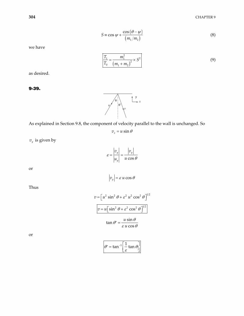
304 CHAPTER 9
1 2
coscosS
m m (8)
we have
2
21 12
0 1 2
T mS
T m m (9)
as desired.
9-39.
#$#
uv
yx
As explained in Section 9.8, the component of velocity parallel to the wall is unchanged. So
sinxv u
yv is given by
cos
y y
y
v v
uu
or
cosyv u
Thus
1 22 2 2 2 2sin cosv u u
1 22 2 2sin cosv u
sin
tancos
uu
or
1 1tan tan
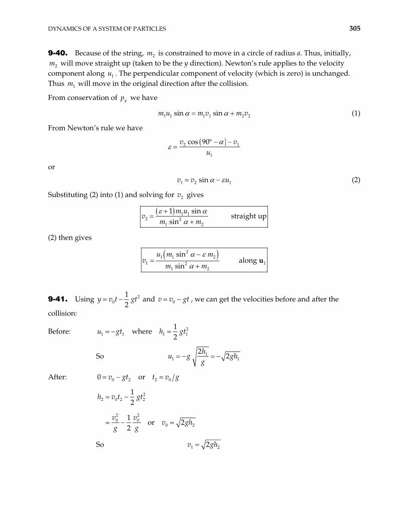
DYNAMICS OF A SYSTEM OF PARTICLES 305
9-40. Because of the string, is constrained to move in a circle of radius a. Thus, initially, will move straight up (taken to be the y direction). Newton’s rule applies to the velocity
component along . The perpendicular component of velocity (which is zero) is unchanged. Thus will move in the original direction after the collision.
2m
2m
1u
1m
From conservation of yp we have
1 1 1 1 2 2sin sinm u m v m v (1)
From Newton’s rule we have
2 1
1
cos 90v vu
or
1 2 sinv v u1 (2)
Substituting (2) into (1) and solving for gives 2v
1 12 2
1 2
1 sinstraight up
sinm u
m mv
(2) then gives
2
1 1 21 12
1 2
sinalong
sin
u m m
m muv
9-41. Using 20
12
y v t gt and v v , we can get the velocities before and after the
collision:
0 gt
Before: 21 1 1
1where
2u gt h g 1t
So 11 1
22
hu g gh
g
After: 0 2 2 00 orv gt t v g
22 0 2 2
2 20 0
0 2
12
1or 2
2
h v t gt
v vv g
g gh
So 1 22v gh
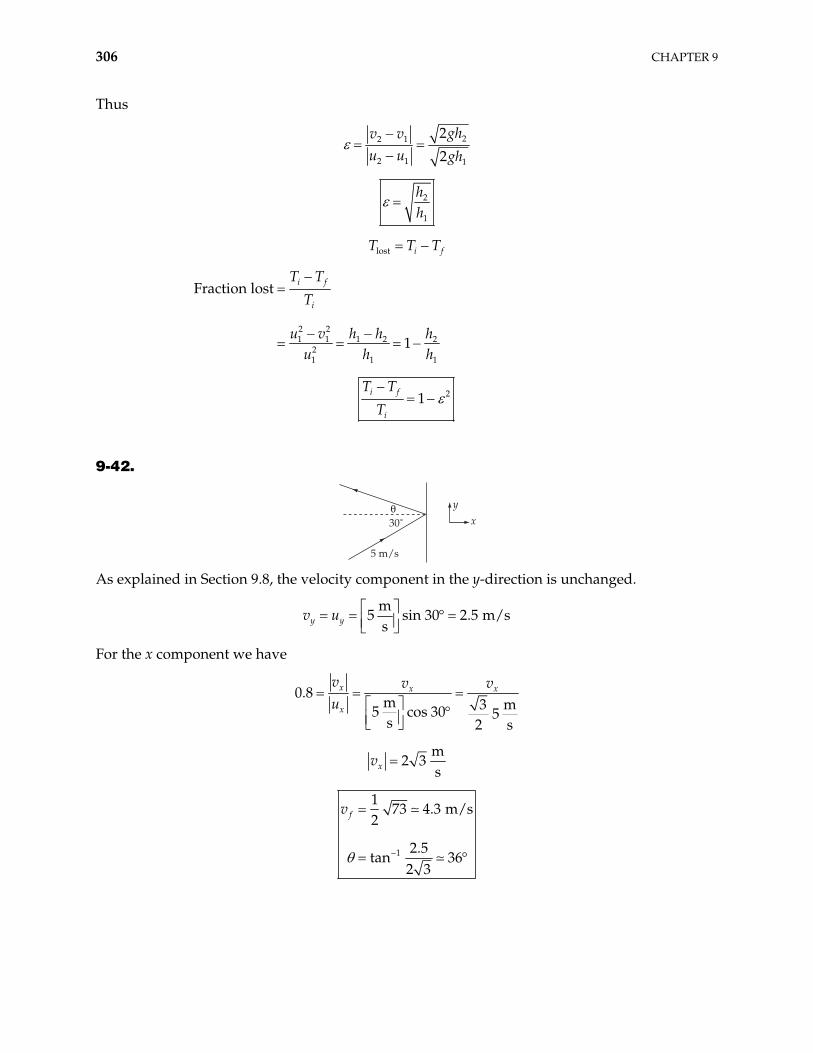
306 CHAPTER 9
Thus
22 1
2 1 1
22
ghv vu u gh
2
1
hh
lost i fT T T
2 21 1 1 2
21 1
Fraction lost
1
i f
i
T T
T
u v h h hu h
2
1h
21i f
i
T T
T
9-42.
yx30˚
5 m/s
#
As explained in Section 9.8, the velocity component in the y-direction is unchanged.
m
5 sin 30 2.5 m/ssy yv u
For the x component we have
0.8m 3 m5 cos 30 5s 2 s
x x x
x
v v vu
m
2 3sxv
1
173 4.3 m/s
2
2.5tan 36
2 3
fv
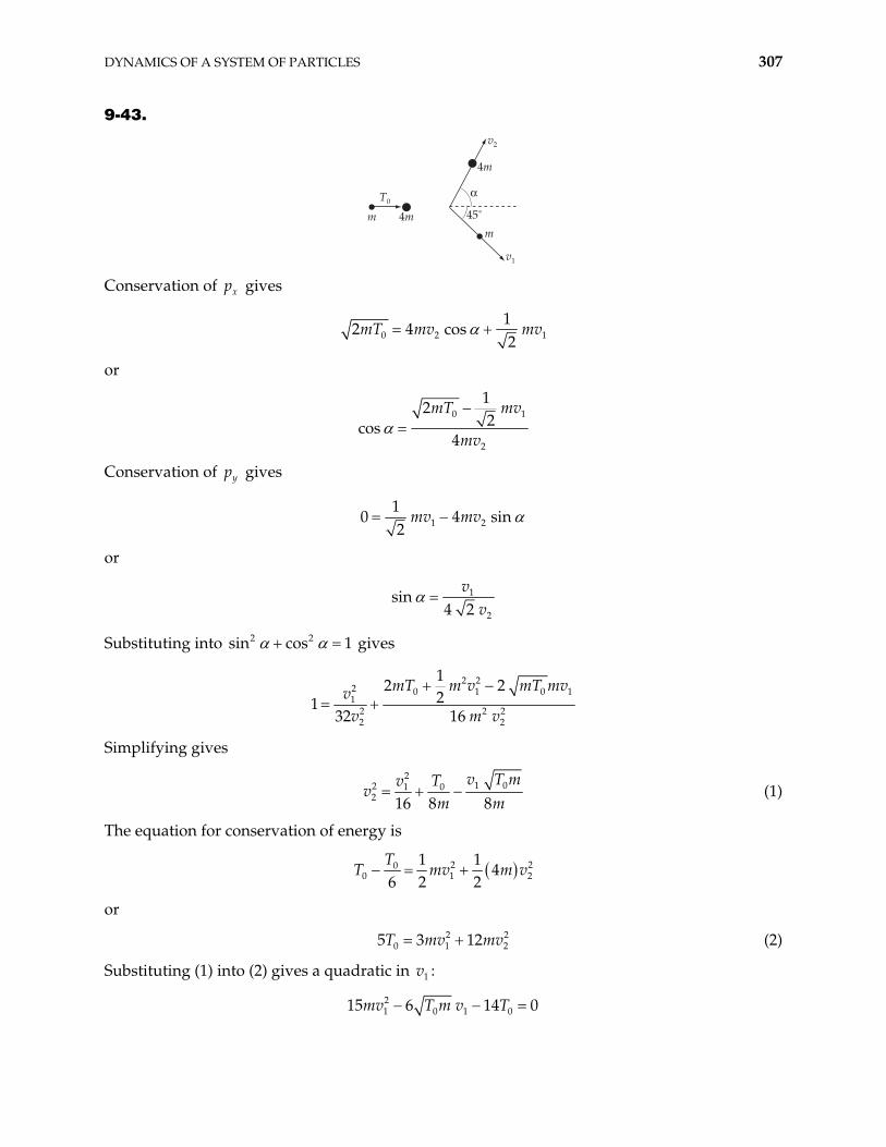
DYNAMICS OF A SYSTEM OF PARTICLES 307
9-43.
%T0
v2
v1
45˚4mmm
4m
Conservation of gives xp
0 21
2 4 cos2
mT mv mv1
or
0 1
2
122cos
4
mT mv
mv
Conservation of yp gives
1 21
0 42
mv mv sin
or
1
2
sin4 2
vv
Substituting into si gives 2 2n cos 1
2 22 0 1 01
2 2 22 2
12 22
32 16
mT m v mT mvvv m v
11
Simplifying gives
2
1 02 012 16 8 8
v T mTvv
m m (1)
The equation for conservation of energy is
2 200 1
1 14
6 2 2T
T mv 2m v
22
or
(2) 20 15 3 12T mv mv
Substituting (1) into (2) gives a quadratic in : 1v
21 0 1 015 6 14 0mv T m v T
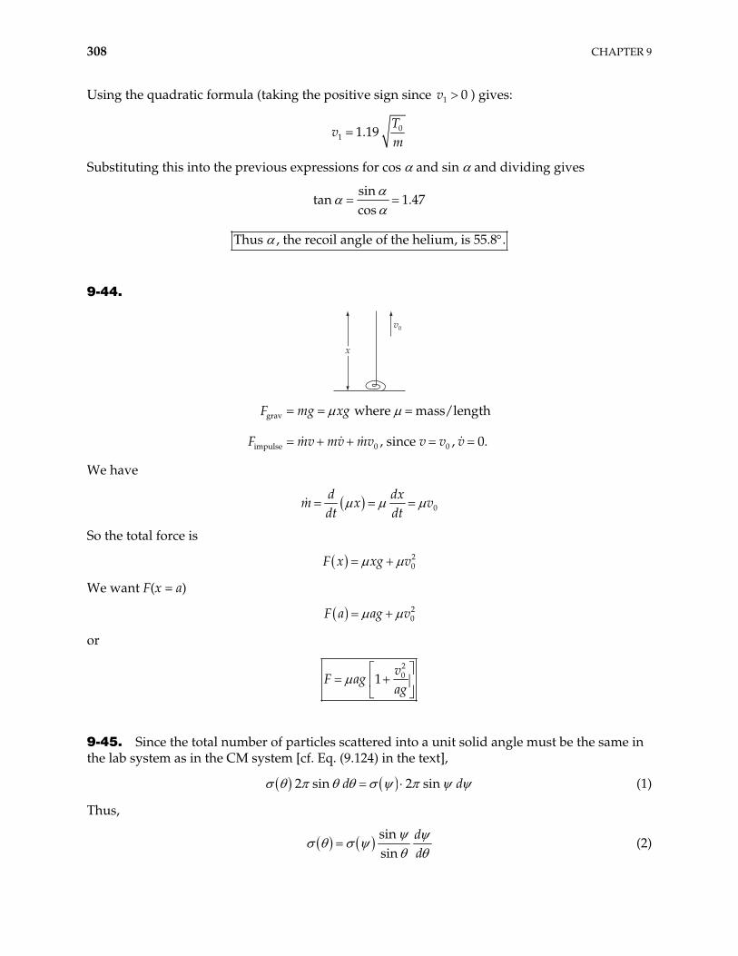
308 CHAPTER 9
Using the quadratic formula (taking the positive sign since v ) gives: 1 0
01 1.19
Tv
m
Substituting this into the previous expressions for cos and sin and dividing gives
sin
tan 1.47cos
Thu s , the recoil angle of the helium, is 55.8 .
9-44.
v0
x
grav
impulse 0 0
where mass/length
, since , 0.
F mg xg
F mv mv mv v v v
We have
0d dx
m xdt dt
v
So the total force is
20F x xg v
We want F(x = a)
20F a ag v
or
201
vF ag
ag
9-45. Since the total number of particles scattered into a unit solid angle must be the same in the lab system as in the CM system [cf. Eq. (9.124) in the text],
2 sin 2 sind d (1)
Thus,
sinsin
dd
(2)
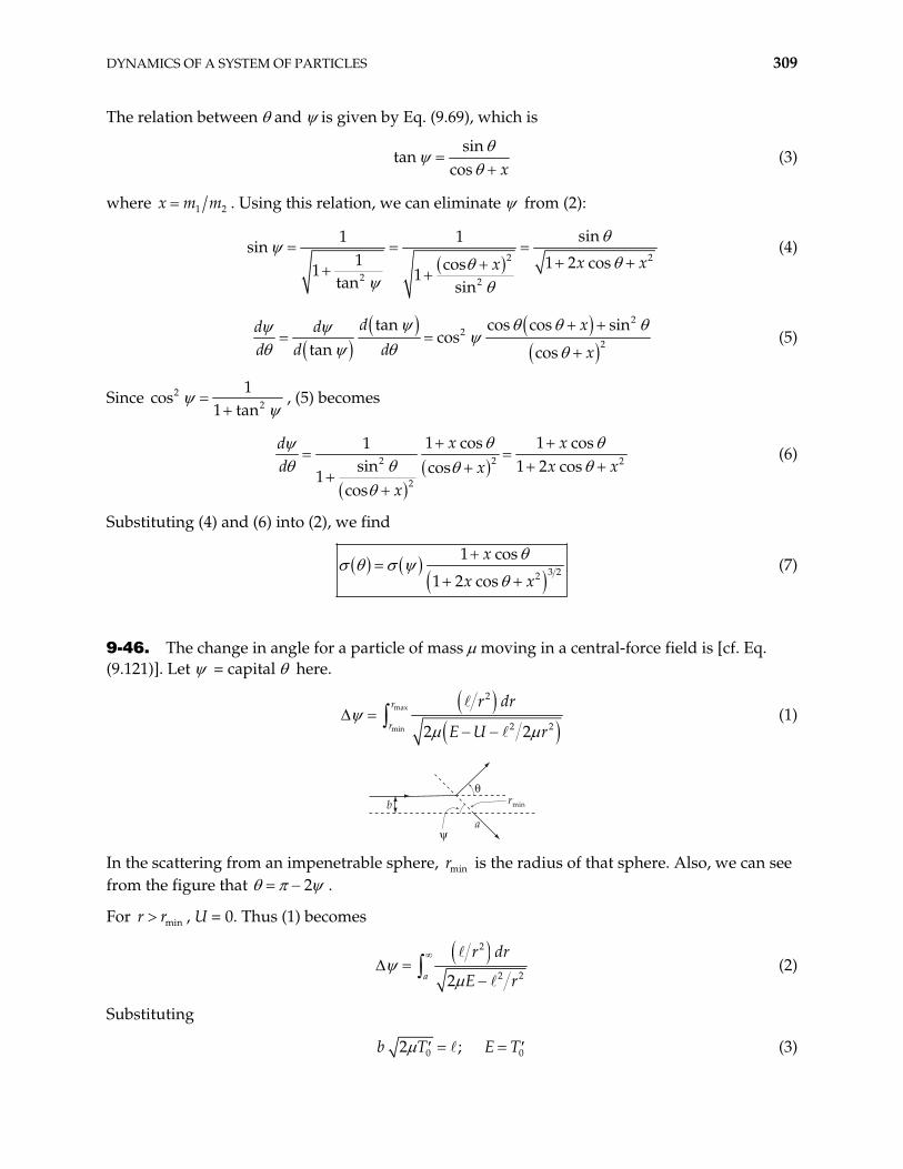
DYNAMICS OF A SYSTEM OF PARTICLES 309
The relation between and is given by Eq. (9.69), which is
sin
tancos x
(3)
where 1x m m2 . Using this relation, we can eliminate from (2):
2
2 2
sin1 1n
1 1 2 coscos1 1tan sinx xx 2
si (4)
2
22
tan cos cos sincos
tan cos
d xd d d x
d d (5)
Since 22
1s
1 tanco , (5) becomes
2 2 2
2
1 cos 1 cos1sin 1 2 coscos1
cos
x xd xx
x
dx
(6)
Substituting (4) and (6) into (2), we find
3 22
1 cos
1 2 cos
x
x x (7)
9-46. The change in angle for a particle of mass moving in a central-force field is [cf. Eq. (9.121)]. Let = capital here.
max
min
2
2 22 2
r
r
r dr
E U r (1)
b
a
rmin
#
( In the scattering from an impenetrable sphere, is the radius of that sphere. Also, we can see from the figure that
minr2 .
For , U = 0. Thus (1) becomes minr r
2
2 22a
r dr
E r (2)
Substituting
02 ;b T E T0 (3)
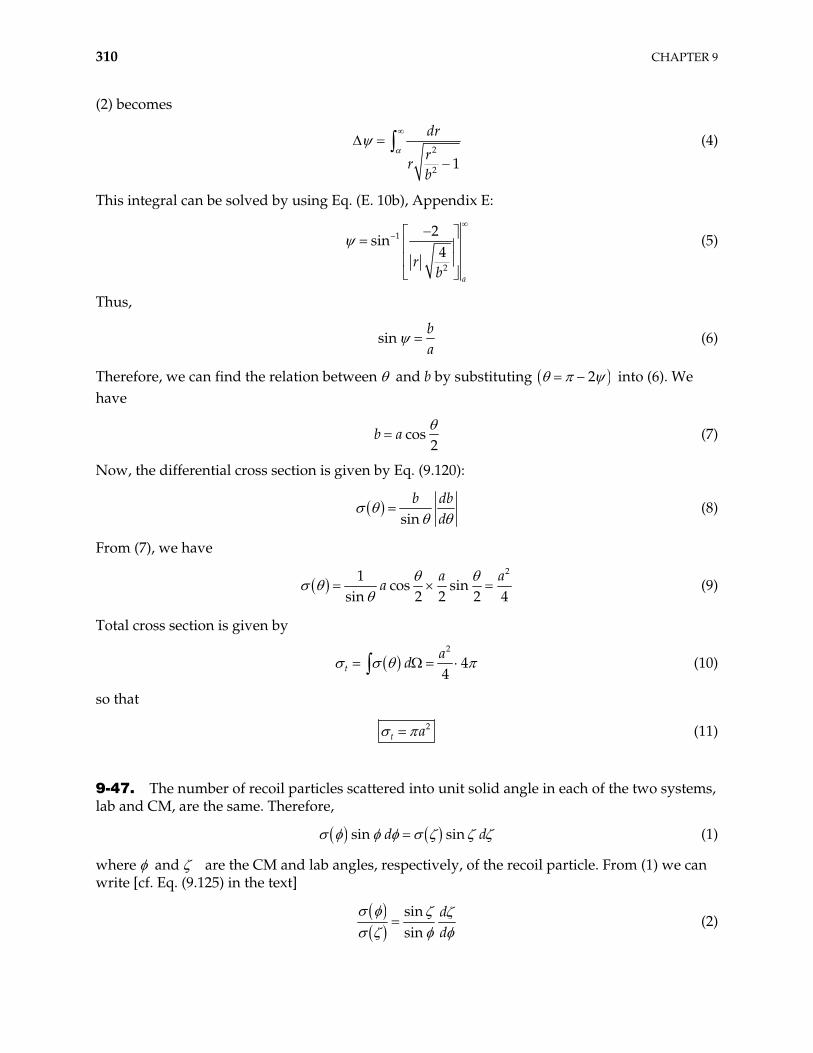
310 CHAPTER 9
(2) becomes
2
2 1
dr
rrb
(4)
This integral can be solved by using Eq. (E. 10b), Appendix E:
1
2
2sin
4
a
rb
(5)
Thus,
sinba
(6)
Therefore, we can find the relation between and b by substituting 2 into (6). We have
cos2
b a (7)
Now, the differential cross section is given by Eq. (9.120):
sin
b dbd
(8)
From (7), we have
21
cos sinsin 2 2 2 4
aa
a (9)
Total cross section is given by
2
44ta
d (10)
so that
2t a (11)
9-47. The number of recoil particles scattered into unit solid angle in each of the two systems, lab and CM, are the same. Therefore,
sin sind d (1)
where and are the CM and lab angles, respectively, of the recoil particle. From (1) we can write [cf. Eq. (9.125) in the text]
sinsin
dd
(2)
DYNAMICS OF A SYSTEM OF PARTICLES 311
Now, in general, 2 [see Eq. (9.74)]. Hence,
sin sin 1sin sin 2 2 cos
(3)
and
12
dd
(4)
Using (3) and (4) in (2), we have
1
4 cos (5)
For , the Rutherford scattering cross section is [Eq. (9.141)] 1m m2
2
2 40
14 sinkT 2
(6)
Also for this case, we have [Eqs. (9.71) and (9.75)]
2
2
(7)
Hence,
sin sin sin cos2 2
(8)
and since the CM recoil cross section ( ) is the same as the CM scattering cross section ( ) , (6) becomes
2
2 40
14 coskT
(9)
Using (5) to express ( ), we obtain
4 cos (10)
or,
2
2 30
1cos
kT
(11)
312 CHAPTER 9
9-48. In the case , the scattering angle for the incident particle measured in the lab system is very small for all energies. We can then anticipate that ( ) will rapidly approach zero as increases.
1m m2
Eq. (9.140) gives the Rutherford cross section in terms of the scattering angle in the CM system:
2
CM 2 40
1sin 24
kT
(1)
From Eq. (9.79) we see that for , 1 2m m
20 0
1 2 1
m mT T
m m m2
0T (2)
Furthermore, from Eq. (9.69),
2
1 1
2
sintan sin
cos
mm mm
(3)
and therefore, since is expected to be small for all cases of interest,
1
2 2
sin tanm mm m
1 (4)
Then,
2
1
2
cos 1mm
(5)
and
2
2 1
2
1sin 2 1 1
2mm
(6)
(Notice that 1 , but since m , the quantity 1 m2 1m m2 is not necessarily small compared to unity.)
With the help of (2) and (6), we can rewrite the CM cross section in terms of as
2
1CM 2
22 01
2
12
1 1
m km T
mm
(7)
According to Eq. (9.129),
DYNAMICS OF A SYSTEM OF PARTICLES 313
22
1 1
2 2
LAB CM 2
1
2
cos 1 sin
1 sin
m mm m
mm
(8)
We can compute LAB with the help of (7) and the simplifications introduced in the right-hand side of (8) by the fact that 1 :
22
1 1
22 2
1LAB 2
2 22 01 1
2 2
1
21 1 1
m mm mm k
m Tm mm m
(9)
and so,
22 2
1 2 0LAB 2
2 2
1 1
2 2
2
1 1 1
m k m T
m mm m
(10)
This expression shows that the cross section has a second-order divergence at = 0. For values of 2m m1 , (9) gives complex values for lab . This result is due to the approximations involved in its derivation, making our result invalid for angles larger than 2 1m m .
9-49. The differential cross section for Rutherford scattering in the CM system is [cf. Eq. (9.140) in the text]
2
240
116 sin
2
kT
(1)
where [cf. Eq. (9.79)]
20
1 2
mT
m m 0T (2)
314 CHAPTER 9
Thus,
221 2
240 2
221
240 2
116 sin
2
11
16 sin2
m mkT m
mkT m
(3)
Since 1 2 1m m , we expand
2
1 1
2 2
1 1 2m mm m
(4)
Thus, to the first order in 1m m2 , we have
2
12
40 2
11 2
16 sin2
mkT m
(5)
This result is the same as Eq. (9.140) except for the correction term proportional to 1 2m m .
9-50. The potential for the given force law is
22k
U rr
(1)
First, we make a change of variable, 1z r . Then, from Eq. (9.123), we can write
max
1 22
max 20
02 2
20
1
2 max 020
220
1
sin2
2
z
kz b
mu
b dz
kb zmu
b zzk
bmu
bk
bmu
(2)
Solving (2) for b = b( ),
2 2 20
2
4
kb
mu (3)
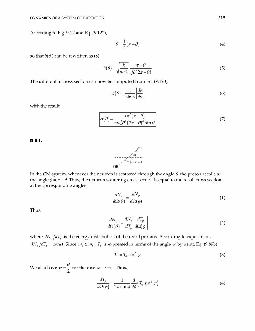
DYNAMICS OF A SYSTEM OF PARTICLES 315
According to Fig. 9-22 and Eq. (9.122),
12
(4)
so that b( ) can be rewritten as ( ):
20 2
kb
mu (5)
The differential cross section can now be computed from Eq. (9.120):
sin
b dbd
(6)
with the result
2
22 20 2 sin
kmu
(7)
9-51.
#
, = * ! #p
n
In the CM system, whenever the neutron is scattered through the angle , the proton recoils at the angle = – . Thus, the neutron scattering cross section is equal to the recoil cross section at the corresponding angles:
pndNdN
d d (1)
Thus,
p pn
p
dN dTdNd dT d
(2)
where p pdN dT is the energy distribution of the recoil protons. According to experiment,
p pdN dT = const. Since p nm m , pT is expressed in terms of the angle by using Eq. (9.89b):
20 sinpT T (3)
We also have 2
for the case p nm m . Thus,
20
1sin
2 sinpdT d
Td d
(4)
316 CHAPTER 9
or,
20
0
sin2 sin 2
sin cos2 sin 2 2 4
pdT T dd d
T T0 (5)
Therefore, we find for the angular distribution of the scattered neutron,
0
4pn
p
dNdN Td dT
(6)
Since p pdN dT = const., ndN d is also constant. That is, the scattering of neutrons by protons is isotropic in the CM system.
9-52. Defining the differential cross section ( ) in the CM system as in Eq. (9.116), the number of particles scattered into the interval from to + d is proportional to
sin cosdN d d
2
(1)
From Eq. (9.87a) and the assumption of elastic collisions (i.e., T T0 1 T ), we obtain
2 1 22
0 1 2
21 cos
T m mT m m
(2)
or, solving for cos ,
22cos m
m
T TT
(3)
where 1 202
1 2
4m
m mm m
T is the maximum energy attainable by the recoil particle in the lab
system. Then, (1) can be rewritten as
T
22m
dTdN
T (4)
and consequently, we obtain the desired result for the energy distribution:
2
dNdT
(5)
DYNAMICS OF A SYSTEM OF PARTICLES 317
9-53.
1m mass of particle 1 , mass of 2m 238 U
1 ,u u1 : velocity of particle in LAB and CM before collision
1 ,v v1
2
2
: velocity of particle in LAB and CM after collision
2 ,u u : velocity of in LAB and CM before collision 238 U
2 ,v v ” velocity of in LAB and CM after collision 238 U
2 0u , 2
1 11 7.7MeV
2m u
T
90 is angle through which particle is deflected in LAB
is angle through which particle and are deflected in CM 238 U
is recoil angle of in LAB 238 U
m1 u1
v1
vv2$ –vCM
m1
m2-
#
2
a) Conservation of momentum in LAB:
1 1 2 21 1
1 1 2 2
costan
sinm u m v
um v m v
v
Conservation of energy in LAB:
2 2
1 1 1 1 2 2
2 2 2m u m v m v2
From these equations we obtain the recoil scattering angle of 238 U
tan 2 1
2 1
44.52m mm m
b) The velocity of CM of system is
1 1CM
1 2
m uv
m m
The velocity of in CM after collision is v v238 U '2 2 Cv M . From the above figure we can obtain
the scattering angle of particle in CM to be 238 U
318 CHAPTER 9
2 2
2 2 12
2 1
sinn 89.04
cos cm
v m mv v m
ta
In CM, clearly after collision, particle moves in opposite direction of that of 23 . 8 U
c) The kinetic energy of particle after collision in LAB is 238 U
22 2 2
1 02 2 2 1 1 11
2 1 2 1 2
20.25 MeV
2 2 cosm vm m u m
Tm m m m m
m v
Evidently, conservation of energy is satisfied.
d) The impact parameter in CM is given in Section 9.10.
0
cot2 2k
bT
where 1 2
09q q
k and 20 1 1 2
12
u m u 22T m is the total energy of system in CM,
so 141 2 1 22
0 1 2 1
cot 1.8 10 m4 2q q m m
bm m u
We note that b is the impact parameter of particle with respect to CM, so the impact
parameter of particle with respect to is 238 U 1 2 14
2
1.83 10 m.m m b
m
e) In CM system, the orbit equation of particle is
1 cosr
where 0 corresponds to r rmin
min 1r is closest distance from particle to the center of mass, and
22
1 10
1 1 2 1
4 m u bm k q q m
and
221 10
1 1 2
21 12 0
1 11 2 1
41 2 1 2
41
m u bEE
m k q q m
m u bm u
q q m
1
But the actual minimum distance between particles is
141 2min min
2
0.93 10 m.m m
r rm
DYNAMICS OF A SYSTEM OF PARTICLES 319
f) Using formula
22 2
LAB CM 2 2
cos 1 sin
1 sin
x x
x
where 1
2
mx
m, 90 ,
2
CM 240
14 sin
2
kT
We find this differential cross section in LAB at = 90°:
28 2LAB 90 3.16 10 m
g) Since d
( ) sin d dN
N we see that the ratio of probability is
sin
11.1' sin
9-54. Equation 9.152 gives the velocity of the rocket as a function of mass:
0 00 0
0
ln ln 0
ln
m mv v u v
m m
mp mv mu
m
To maximize p, set 0dpdm
00 lndp m
udm m
1
10 0
0
1m m m
e or em m m
ln
To check that we have a maximum, examine
1
0
2 2
2 2m m e
d p d p udm dm m
1
0
2
20
0m m e
d p ue
dm m, so we have a maximum.
1
0
me
m
320 CHAPTER 9
9-55. The velocity equation (9.165) gives us:
0lnm
v t gt um t
(1)
where 0m t m t , the burn rate 09 10m , the burn time 300 s , and the exhaust
velocity u . These equations are good only from t = 0 to t = . First, let us check that the rocket does indeed lift off at t = 0: the thrust
-14500 m s2
0 09 10 su um m m0 g13 5 m , as required. To find the maximum velocity of the rocket, we need to check it at the times t = 0 and t = , and also check for the presence of any extrema in the region 0 < t < . We have v(0) = 0,
, and calculate 1( ) 0 m sln 10v g u 740
1 0dv u u
g gdt m t m t g
(2)
The inequality follows since 0u m g m t g100 m s
. Therefore the maximum velocity occurs at t = ,
where v g . A similar single-stage rocket cannot reach the moon since ln 10 74u110 4 m s0ln ln 10finalu m m uv t , which is less than escape velocity and independent of
fuel burn rate.
9-56.
a) Since the rate of change of mass of the droplet is proportional to its cross-sectional area, we have
2dmk r
dt (1)
If the density of the droplet is ,
343
m r (2)
so that
24dm dm dr dr
rdt dr dt dt
2kr (3)
Therefore,
4
dr kdt
(4)
or,
0 4k
r r t (5)
as required.
DYNAMICS OF A SYSTEM OF PARTICLES 321
b) The mass changes with time, so the equation of motion is
d dv dm
F mv m v mdt dt dt
g (6)
Using (1) and (2) this becomes
3 24 43 3
dvr kr v
dt3r g (7)
or,
3
4dv k
v gdt r
(8)
Using (5) this becomes
0
34
4
dv k vgkdt r t
(9)
If we set 34
kA and
4k
B , this equation becomes
0
dv Av g
dt r Bt (10)
and we recognize a standard form for a first-order differential equation:
dv
P t v Q tdt
(11)
in which we identify
0
AP t
r Bt; Q(t) = g (12)
The solution of (11) is
v t constantP t dt P t dt
e e Q dt (13)
Now,
00
30
ln
ln
A AP t dt dt r Bt
r Bt B
r Bt (14)
since 3AB
. Therefore,
(15) 30
Pdte r Bt
322 CHAPTER 9
Thus,
3 30 0
3 40 0
constant
4
v t r Bt r Bt g dt
gr Bt r Bt C
B (16)
The constant C can be evaluated by setting 00v t v :
40 03
0
14g
v rr B
C (17)
so that
30 0 04
gC v r r
B4 (18)
We then have
4 30 0 03
0
14 4g g
r Bt v r rB Br Bt
40v t (19)
or,
4 303
10
4g
v t Bt rBBt
(20)
where 30r0 means “terms of order and higher.” If is sufficiently small so that we can
neglect these terms, we have
30r 0r
v t t (21)
as required.
9-57. Start from our definition of work:
dp
W F dx dx v dpdt
(1)
We know that for constant acceleration we must have v = at (zero initial velocity). From Equation (9.152) this means
0at um m e (2)
We can then compute dp:
0 1at u atd mv d mat ma dt at dm m ae dt
udp (3)
This makes our expression for the work done on the rocket
0
0
t at ur
m aW at u at e
udt (4)
DYNAMICS OF A SYSTEM OF PARTICLES 323
The work done on the exhaust, on the other hand, is given with v (v – u) and , so that (exhaustdp dm v u)
20
0
t at ue
m aW at u e
udt (5)
The upper limit on the integrals is the burnout time, which we can take to be the final velocity divided by the acceleration. The total work done by the rocket engines is the sum of these two quantities, so that
2 2000 0
1v a v uat u xm a
u uat e dt m u x e dxu
W (6)
where the obvious substitution was made in the last expression. Upon evaluating the integral we find
0v uW m uve muv (7)
where m is the mass of the rocket after its engines have turned off and v is its final velocity.
9-58. From Eq. (9.165) the velocity is
0lndy m
v gt udt m
0lnm
dy gt u dtm
Since mdt
, dt dm
2 01ln
2mu
y C gt dmm
ln 1 lna a
dx xx x
, so we have
2 01ln
2mu
y C gt m mm
Evaluate C using y = 0 when t = 0, 0m m
0umC
0 2 01ln
2u m m mmu
tm
y g ; 0m m t
2 01ln
2mmu
y ut gtm
At burnout, , By y Bt t
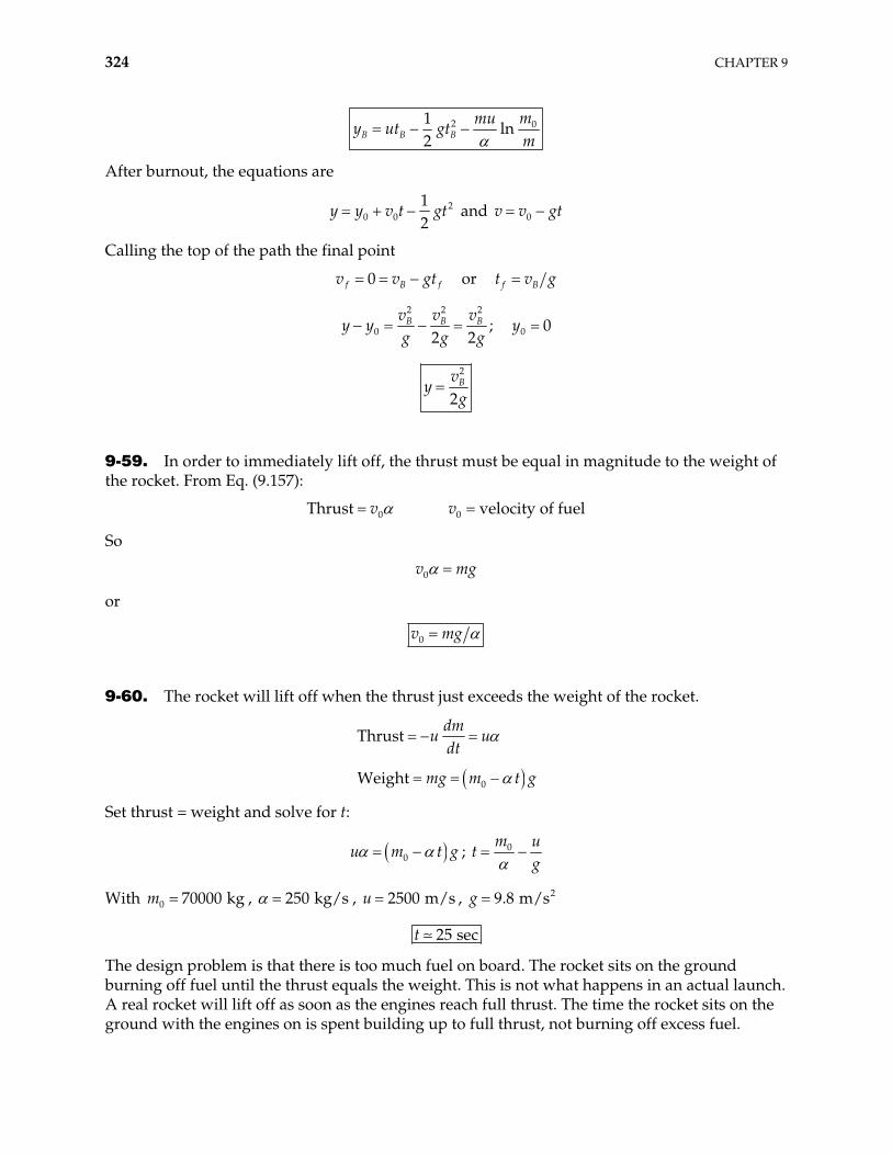
324 CHAPTER 9
2 01ln
2B B Bmmu
y ut gtm
After burnout, the equations are
20 0
12
y y v t gt and v v0 gt
Calling the top of the path the final point
0f B fv v gt or f Bt v g
2 2
0 2 2B Bv v v
y yg g
2B
g; 0 0y
2
2Bv
yg
9-59. In order to immediately lift off, the thrust must be equal in magnitude to the weight of the rocket. From Eq. (9.157):
Thru 0st v 0 velocity of fuelv
So
0v mg
or
0v mg
9-60. The rocket will lift off when the thrust just exceeds the weight of the rocket.
Thrustdm
u udt
0Weight mg m t g
Set thrust = weight and solve for t:
0u m t g ; 0m ut
g
With , 0 70000 kgm 250 kg/s , 2500 m/su , 29.8 m/sg
25 sect
The design problem is that there is too much fuel on board. The rocket sits on the ground burning off fuel until the thrust equals the weight. This is not what happens in an actual launch. A real rocket will lift off as soon as the engines reach full thrust. The time the rocket sits on the ground with the engines on is spent building up to full thrust, not burning off excess fuel.
DYNAMICS OF A SYSTEM OF PARTICLES 325
9-61. From Eq. (9.153), the velocity after the first state is:
1 0 lnv v u k
After the second stage:
2 1 0ln 2 lnv v u k v u k
After the third stage:
3 2 0ln 3 lnv v u k v u k
After the n stages:
1 0ln lnn nv v u k v nu k
0 lnnv v nu k
9-62. To hover above the surface requires the thrust to counteract the gravitational force of the moon. Thus:
16
6
dmu m
dt
u dmdt
g m
g
Integrate from m to 0.8 and t = 0 to T: 0m 0m
2
6 2000 m/s6ln 0.8 ln 0.8
9.8 m/su
Tg
273 secT
9-63.
a) With no air resistance and constant gravity, the problem is simple:
20
12
mv mgh (1)
giving the maximum height of the object as 20 2 1800 kmh v g . The time it takes to do this is
0 610 sv g .
b) When we add the expression for air resistance, the differential equation that describes the projectile’s ascent is
2
211
2 Wt
dv vmg c Av mg
dt vF m (2)
326 CHAPTER 9
where 12 2 5 kt Wg c A
1 3 kg
m sv m would be the terminal velocity if the object were falling
from a sufficient height (using 3m as the density of air). Solution of this differential equation gives
1 0tan tantt t
gtvv t v
v v (3)
This gives v = 0 at time 10tan 300 st tv g v v . The velocity can in turn be integrated to
give the y-coordinate of the projectile on the ascent. The height it reaches is the y-coordinate at time :
22
0ln 12
t
t
v vh
g v (4)
which is 600 km.
c) Changing the acceleration due to gravity from –g to 22
e e e eGM R y g R R y changes our differential equation for y to
22
e
t e
y Ry g
v R y (5)
Using the usual numerical techniques, we find that the projectile reaches a height of 630 km in
a flight time of 330 s.
d) Now we must replace the in the air resistance equation with ( )y . Given the dependence of on , we may write the differential equation tv
22
0
e
t e
y y Ry g
v R y (6)
where we use log and 510 ( ) 0 11 (5 10 )y y 0 1 3 , with the ’s in and y in meters.
The projectile then reaches a height of 2500 km in a flight time of 940 s. This is close to the
height to which the projectile rises when there is no air resistance, which is 2600 km.
3kg m
DYNAMICS OF A SYSTEM OF PARTICLES 327
0 0.1 0.2 0.3 0.4 0.5 0.6 0.7 0.8 0.9 10
0.5
1
1.5
2
2.5
(a) (b) (c) (d)
t (1000 s)
heig
ht (1
000
km)
9-64. We start with the equation of motion for a rocket influenced by an external force, Eq. (9.160), with including gravity, and later, air resistance. extF
a) There is only constant acceleration due to gravity to worry about, so the problem can be solved analytically. From Eq. (9.166), we can obtain the rocket’s height at burnout
2 01ln
2b b bb
mmuy ut gt
m (1)
where is the mass of the rocket at burnout and bm 0 bm m tb . Substitution of the given
values gives . After burnout, the rocket travels an additional 250 kmby 2 2bv , where is the
rocket velocity at burnout. The final height the rocket ends up being 3700 km, after everything is taken into account.
g bv
b) The situation, and hence the differential equation, becomes more complicated when air resistance is added. Substituting 2 2ext WF mg c Av (with ) into Equation (9.160), we obtain
31 3 kg m
2
2Wc Avdv u
gdt m m
(2)
We must remember that the mass m is also a function of time, and we must therefore include it also in the system of equations. To be specific, the system of equations we must use to do this by computer are
2
2W
vy
c Avuv g
m mm
(3)
These must be integrated from the beginning until the burnout time, and therefore must be integrated with the substitution = 0. Firstly, we get the velocity and height at burnout to be
and . We can numerically integrate to get the second part of the 17000 m sbv 230 kmby
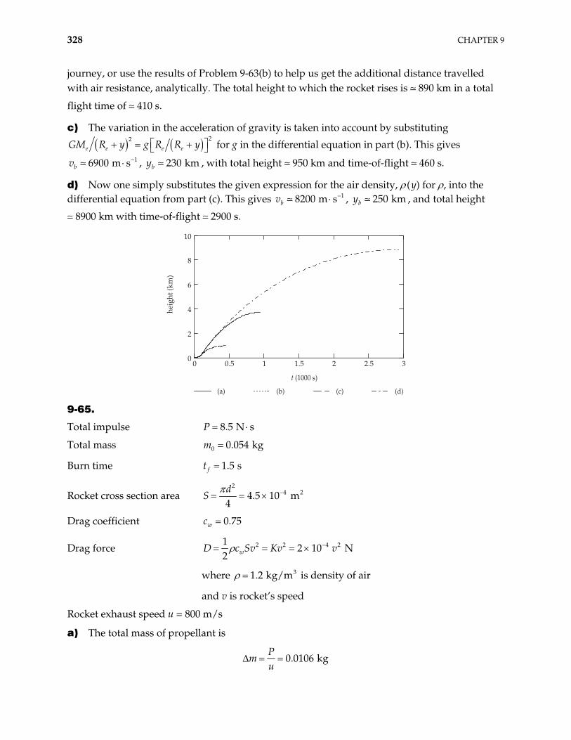
328 CHAPTER 9
journey, or use the results of Problem 9-63(b) to help us get the additional distance travelled with air resistance, analytically. The total height to which the rocket rises is 890 km in a total
flight time of 410 s.
c) The variation in the acceleration of gravity is taken into account by substituting 22
e e e eGM R y g R R y16900 m sbv 230 kmby
for g in the differential equation in part (b). This gives
, , with total height 950 km and time-of-flight 460 s.
d) Now one simply substitutes the given expression for the air density, (y) for , into the differential equation from part (c). This gives v 18200 m sb , , and total height
8900 km with time-of-flight 2900 s.
250 kmby
0 0.5 1 1.5 2 2.5 30
2
4
6
8
10
heig
ht (k
m)
(a) (b) (c) (d)
t (1000 s)
9-65.
Total impulse 8.5 N sP
Total mass 0 0.054 kgm
Burn time 1.5 sft
Rocket cross section area 2
4 24.5 10 m4d
S
Drag coefficient 0.75wc
Drag force 2 2 4 212 10 N
2 wD c Sv Kv v
where 1.2 is density of air 3 kg/m
and v is rocket’s speed
Rocket exhaust speed u = 800 m/s
a) The total mass of propellant is
0.0106 kgP
mu
DYNAMICS OF A SYSTEM OF PARTICLES 329
Since , we will assume that the rocket’s mass is approximately constant in this problem. The equation of motion of rocket is
0~ 20%m m
20 o
dvm m g u
dtKv
(where 37.1 10 kg/sf
mt
is fuel burn rate)
02
0
m dvdt
u m g Kv
Using the initial condition at t = 0, v = 0, we find
0 02
0
( ) tanhu m g K u m g
K mv t
At burn-out, , we find 1.5 sft t
( ) 114.3 m/sf fv v t
The height accordingly is given by
00200
( ) ( ) d ln coshk u m gm
v t t tk m
h t
At burn out, ft t , we find the burn-out height
( ) 95.53 mf fh h t
b) After the burn-out, the equation of motion is
2 00 0 2
0
ddd
dm vv
g Kvt m g
m m tKv
with solution
0
0
( ) tanm g Kg
v t t CK m
Using the initial condition at ft t , ft vv , we find the constant C = –1.43 rad, so
0
0
( ) tan 1.43m g Kg
v t tK m
and the corresponding height
0
0
( ) ( ) d 0.88 ln cos 1.43f
t
f ft
Kgmh v t t h t
K mh t
330 CHAPTER 9
When the rocket reaches its maximum height (at t tmax ) the time t can be found by setting We then find And the maximum height the rocket can reach is
max
max( )v t 0. max 7.52 s.t
max max( ) 334 mh h t
c) Acceleration in burn-out process is (see v(t) in a))
0
0 0220
d 1( )
dcosh
u m gvt m k u m g
tm
a t
Evidently, the acceleration is maximum when t = 0 and
20
0
( 0) 95.4 m/smaxu m g
a a tm
d) In the fall-down process, the equation of motion is
200
dd
m vm g Kv
t,
With the initial condition t t , v = 0, we find max maxt t
0max
0
( ) tanhm g Kg
v t t tK m
(v(t) is negative for , because then the rocket falls downward) maxt t
The height of the rocket is
max
0max max max
0
( ) ln cosht
t
Kgmv t dt h t t
K mh h
To find the total flight-time, we set h = 0 and solve for t. We find total 17.56 st
e) Putting into the expression of V in part d), we find the speed at ground impact to be
totalt t t
0max
0
tanh 49.2 m/sg totalm g Kg
tK m
v t
9-66. If we take into account the change of the rocket’s mass with time 0m m t , where is the fuel burn rate,
37.1 10 kg/s
as calculated in problem 9-65.
The equation of motion for the rocket during boost phase is
DYNAMICS OF A SYSTEM OF PARTICLES 331
20 2
0
d dd
v vm t u Kv
t Kv udt
t m
Integrating both sides we obtain finally
2
0
20
1( )
1
Ku
Ku
C t m uv t
KC t m
where C is a constant. Using the initial condition ( ) 0 at 0v t t , we can find C and the velocity is
2
0
2
0
1 1( )
1 1
Ku
Ku
tmu
v tK
tm
a) The rocket speed at burn-out is (note t 1.5 sf ).
( ) 131.3 m/sf fv v t
b) The distance the rocket has traveled to the burn-out is
( ) 108.5 mft
fh v t dt
9-67. From Equation (9.167) we have
2
002
0
ln2
f fbo f f
g m m muH m m
mm
Using numerical values from Example 9.12 41.42 10 kg/s
60 2.8 10 kgm
60.7 10 kgfm
2.600 m/su
we find 97.47 kmboH .
From Equation (9.168) we find
0( )lnf o
bof
g m m mv u
m
2125 m/sbov

332 CHAPTER 9
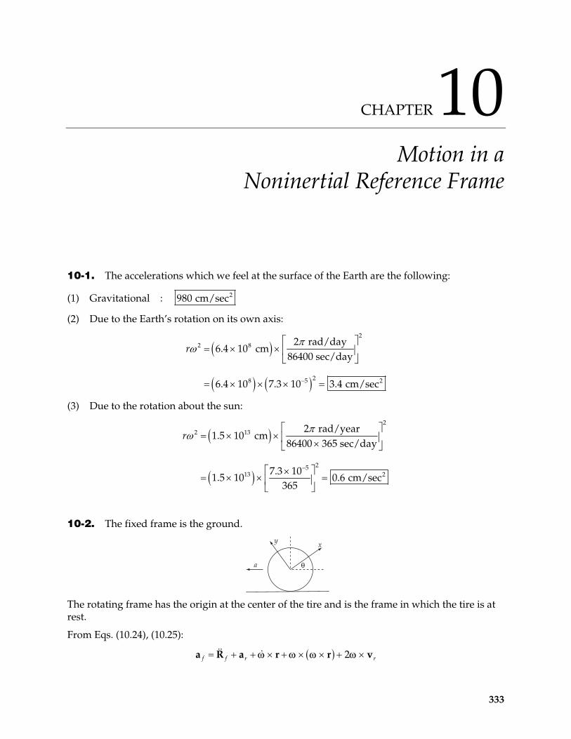
CHAPTER 10 Motion in a
Noninertial Reference Frame
10-1. The accelerations which we feel at the surface of the Earth are the following:
(1) Gravitational : 2980 cm/sec
(2) Due to the Earth’s rotation on its own axis:
2
2 8
28 5
2 rad/day6.4 10 cm
86400 sec/day
6.4 10 7.3 10 3.4 cm/sec
r
2
(3) Due to the rotation about the sun:
22 13
2513 2
2 rad/year1.5 10 cm
86400 365 sec/day
7.3 101.5 10 0.6 cm/sec
365
r
10-2. The fixed frame is the ground.
y
a !
x
The rotating frame has the origin at the center of the tire and is the frame in which the tire is at rest.
From Eqs. (10.24), (10.25):
2f f r ra r r va R
333
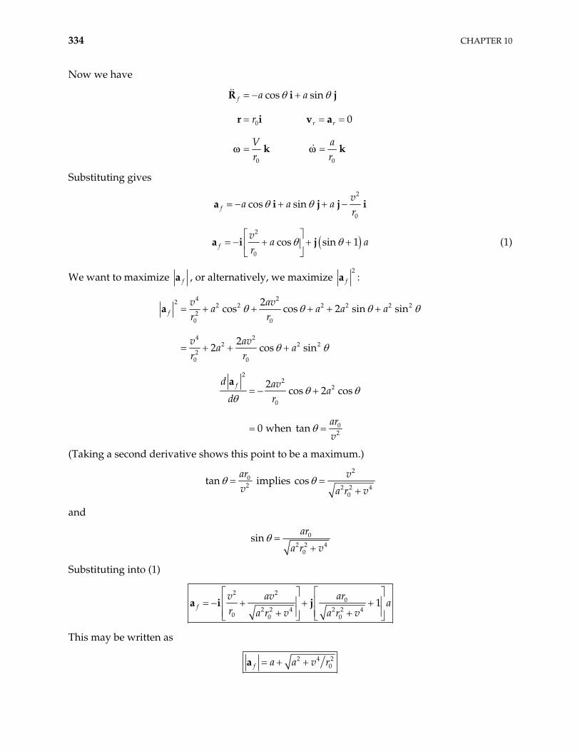
334 CHAPTER 10
Now we have
0
0 0
cos sin
0
f
r r
a a
r
V ar r
R i
r i v a
k k
j
Substituting gives
2
0
cos sinfv
a a ar
a i j j i
2
0
cos sin 1fv
ar
a i j a (1)
We want to maximize fa , or alternatively, we maximize 2
fa :
4 22 2 2 2 2 2 22
0 0
4 22 2 2
20 0
2cos cos 2 sin sin
22 cos sin
fv av
a a ar r
v ava a
r r
aa
22
2
0
02
2cos 2 cos
0 when tan
fd ava
d r
arv
a
(Taking a second derivative shows this point to be a maximum.)
2
02 2 2 4
0
n implies cosar vv a r v
ta
and
02 2 4
0
sinar
a r v
Substituting into (1)
2 2
02 2 4 2 2 4
0 0 0
1farv av
ar a r v a r v
ja i
This may be written as
2 4 20f a a v ra
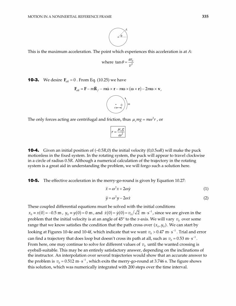
MOTION IN A NONINERTIAL REFERENCE FRAME 335
!
A
This is the maximum acceleration. The point which experiences this acceleration is at A:
where 02
arv
tan
10-3. We desire . From Eq. (10.25) we have eff 0F
eff 2f rm m m mr r vF F R
r
0 "
The only forces acting are centrifugal and friction, thus 2smg m r , or
2s gr
10-4. Given an initial position of (–0.5R,0) the initial velocity (0,0.5 R) will make the puck motionless in the fixed system. In the rotating system, the puck will appear to travel clockwise in a circle of radius 0.5R. Although a numerical calculation of the trajectory in the rotating system is a great aid in understanding the problem, we will forgo such a solution here.
10-5. The effective acceleration in the merry-go-round is given by Equation 10.27:
2 2x x y (1)
2 2y y x (2)
These coupled differential equations must be solved with the initial conditions
0 0 0.5 mx x , 0 0 0 my y , and 100 0 2 m sx y v
0v
, since we are given in the problem that the initial velocity is at an angle of 45° to the x-axis. We will vary over some range that we know satisfies the condition that the path cross over . We can start by
looking at Figures 10-4e and 10-4f, which indicate that we want . Trial and error can find a trajectory that does loop but doesn’t cross its path at all, such as
0v
1
0.
0 0( , )x y
0.47 m s
0v 153 m s . From here, one may continue to solve for different values of v until the wanted crossing is eyeball-suitable. This may be an entirely satisfactory answer, depending on the inclinations of the instructor. An interpolation over several trajectories would show that an accurate answer to the problem is , which exits the merry-go-round at 3.746 s. The figure shows this solution, which was numerically integrated with 200 steps over the time interval.
0
10.512 m s0v
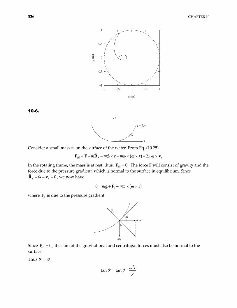
336 CHAPTER 10
–0.5 0 0.5 1
0.5
0
0.5
x (m)y
(m)
1
–1–1
10-6.
z
m
r
z = f(r)
Consider a small mass m on the surface of the water. From Eq. (10.25)
eff 2f rm m m r mr vF F R
In the rotating frame, the mass is at rest; thus, eff 0F . The force F will consist of gravity and the force due to the pressure gradient, which is normal to the surface in equilibrium. Since
, we now have 0f rR v
0 pm mg F r
where pF is due to the pressure gradient.
Fp
mg
m"2r
!#
!
Since F , the sum of the gravitational and centrifugal forces must also be normal to the surface.
eff 0
Thus = .
2
tan tanr
g
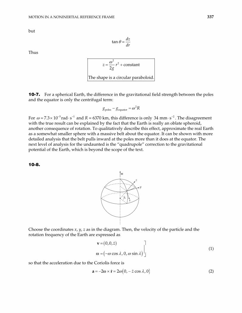
MOTION IN A NONINERTIAL REFERENCE FRAME 337
but
tandzdr
Thus
22 constant
2
The shape is a circular paraboloid.
z rg
10-7. For a spherical Earth, the difference in the gravitational field strength between the poles and the equator is only the centrifugal term:
2poles equatorg g R
For and R = 6370 km, this difference is only 3457.3 10 rad s 1 2 mm s . The disagreement with the true result can be explained by the fact that the Earth is really an oblate spheroid, another consequence of rotation. To qualitatively describe this effect, approximate the real Earth as a somewhat smaller sphere with a massive belt about the equator. It can be shown with more detailed analysis that the belt pulls inward at the poles more than it does at the equator. The next level of analysis for the undaunted is the “quadrupole” correction to the gravitational potential of the Earth, which is beyond the scope of the text.
10-8.
x
y
z
$
"
Choose the coordinates x, y, z as in the diagram. Then, the velocity of the particle and the rotation frequency of the Earth are expressed as
0,0,
cos , 0, sin
zv (1)
so that the acceleration due to the Coriolis force is
2 2 0, cosza r , 0 (2)
338 CHAPTER 10
This acceleration is directed along the y axis. Hence, as the particle moves along the z axis, it will be accelerated along the y axis:
2 cosy z (3)
Now, the equation of motion for the particle along the z axis is
0z v gt (4)
20
12
z v t gt (5)
where v is the initial velocity and is equal to 0 2gh if the highest point the particle can reach is h:
0 2v gh
c
(6)
From (3), we have
2 cosy z (7)
but the initial condition 0y z 0 implies c = 0. Substituting (5) into (7) we find
20
2 20
12 cos
2
cos 2
y v t
gt v t
gt
(8)
Integrating (8) and using the initial condition y(t = 0) = 0, we find
2 20
1cos
3y gt v t (9)
From (5), the time the particle strikes the ground (z = 0) is
01
02
v gt t
so that
02vt
g (10)
Substituting this value into (9), we have
3 20 0
03 2
302
8 41cos
3
4cos
3
v vy g v
g g
vg
(11)
If we use (6), (11) becomes
MOTION IN A NONINERTIAL REFERENCE FRAME 339
34
cos3
hy
g8
(12)
The negative sign of the displacement shows that the particle is displaced to the west.
10-9. Choosing the same coordinate system as in Example 10.3 (see Fig. 10-9), we see that the lateral deflection of the projectile is in the x direction and that the acceleration is
02 2 sin cosx z ya x v V (1)
Integrating this expression twice and using the initial conditions, 0x 0 and 0x 0 , we obtain
20 cos sinx t V t (2)
Now, we treat the z motion of the projectile as if it were undisturbed by the Coriolis force. In this approximation, we have
20
1sin
2z t V t gt (3)
from which the time T of impact is obtained by setting z = 0:
02 sinVT
g (4)
Substituting this value for T into (2), we find the lateral deflection at impact to be
3
202
4sin cos sin
Vx T
g (5)
10-10. In the previous problem we assumed the z motion to be unaffected by the Coriolis force. Actually, of course, there is an upward acceleration given by 2 x yv so that
02 cos cosz V g (1)
from which the time of flight is obtained by integrating twice, using the initial conditions, and then setting z = 0:
0
0
2 sin2 cos cos
VT
g V (2)
Now, the acceleration in the y direction is
0
2
2 cos sin
y x za y v
V gt (3)
Integrating twice and using the initial conditions, 00 cosy V and 0 0y , we have
340 CHAPTER 10
3 20
1cos cos sin cos
3t gt V t V t0y (4)
Substituting (2) into (4), the range R is 3 3 3 3 2
0 0 03 2
00 0
sin cos 4 sin cos 2 cos cos83 22 cos cos 2 cos cos
V g V VR
g Vg V g V cos cos (5)
We now expand each of these three terms, retaining quantities up to order but neglecting all quantities proportional to 2 and higher powers of . In the first two terms, this amounts to neglecting 02 cos cV os compared to g in the denominator. But in the third term we must use
2 20 0 0
0
320
0 2
2 cos sin 2 2cos sin 1 cos cos
21 cos cos
4sin cos cos
V V Vg gV
gg
VR
g (6)
where is the range when Coriolis effects are neglected [see Example 2.7]: 0R
2
00
2cos sin
VR
g (7)
The range difference, , now becomes 0R R R
3
202
4 1cos sin cos sin
3V
Rg
3 (8)
Substituting for in terms of from (7), we have, finally, 0V 0R
1 2 3 202 1cos cot tan
3R
Rg
(9)
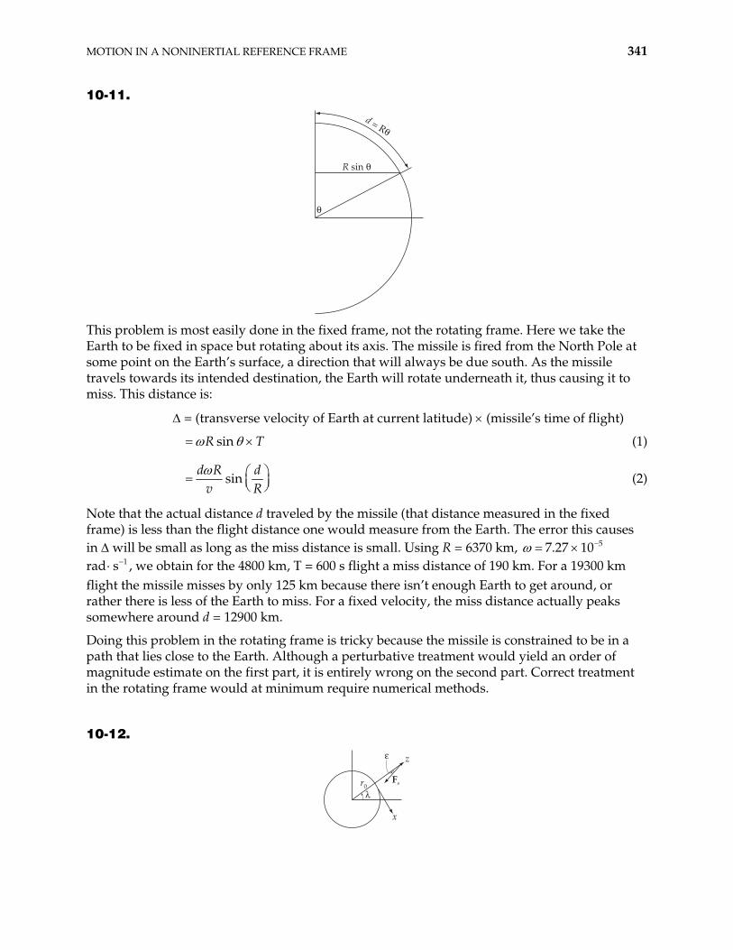
MOTION IN A NONINERTIAL REFERENCE FRAME 341
10-11.
!
R sin !
d = R!
This problem is most easily done in the fixed frame, not the rotating frame. Here we take the Earth to be fixed in space but rotating about its axis. The missile is fired from the North Pole at some point on the Earth’s surface, a direction that will always be due south. As the missile travels towards its intended destination, the Earth will rotate underneath it, thus causing it to miss. This distance is:
= (transverse velocity of Earth at current latitude) (missile’s time of flight)
sinR T (1)
sind R d
v R (2)
Note that the actual distance d traveled by the missile (that distance measured in the fixed frame) is less than the flight distance one would measure from the Earth. The error this causes in will be small as long as the miss distance is small. Using R = 6370 km, 57.27 10 rad , we obtain for the 4800 km, T = 600 s flight a miss distance of 190 km. For a 19300 km flight the missile misses by only 125 km because there isn’t enough Earth to get around, or rather there is less of the Earth to miss. For a fixed velocity, the miss distance actually peaks somewhere around d = 12900 km.
1s
Doing this problem in the rotating frame is tricky because the missile is constrained to be in a path that lies close to the Earth. Although a perturbative treatment would yield an order of magnitude estimate on the first part, it is entirely wrong on the second part. Correct treatment in the rotating frame would at minimum require numerical methods.
10-12.
z
Fsr0
x
$
%
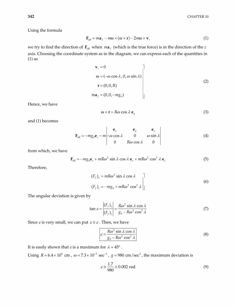
342 CHAPTER 10
Using the formula
eff 2f rm m mF a r v (1)
we try to find the direction of when effF fma (which is the true force) is in the direction of the z axis. Choosing the coordinate system as in the diagram, we can express each of the quantities in (1) as
0
0
( cos , 0, sin )
(0,0, )
(0,0, )
r
f
R
m mg
v
r
a
(2)
Hence, we have
cos yRr e (3)
and (1) becomes
eff 0 cos 0 sin0 cos 0
x y
zmg mR
ze e e
2 2
F e (4)
from which, we have
2eff 0 sin cos cosz xmg mR mR zeF e (5) e
Therefore,
2
2 20
( ) sin cos
( ) cos
f x
f z
F mR
F mg mR (6)
The angular deviation is given by
2
2 20
( ) sin costan
cos( )f x
f z
F Rg RF
(7)
Since is very small, we can put . Then, we have
2
2 20
sin coscos
Rg R
(8)
It is easily shown that is a maximum for 45 .
Using , , , the maximum deviation is 86.4 10 cmR 5 17.3 10 sec 2980 cm/secg
1.7
0.002 rad980
(9)
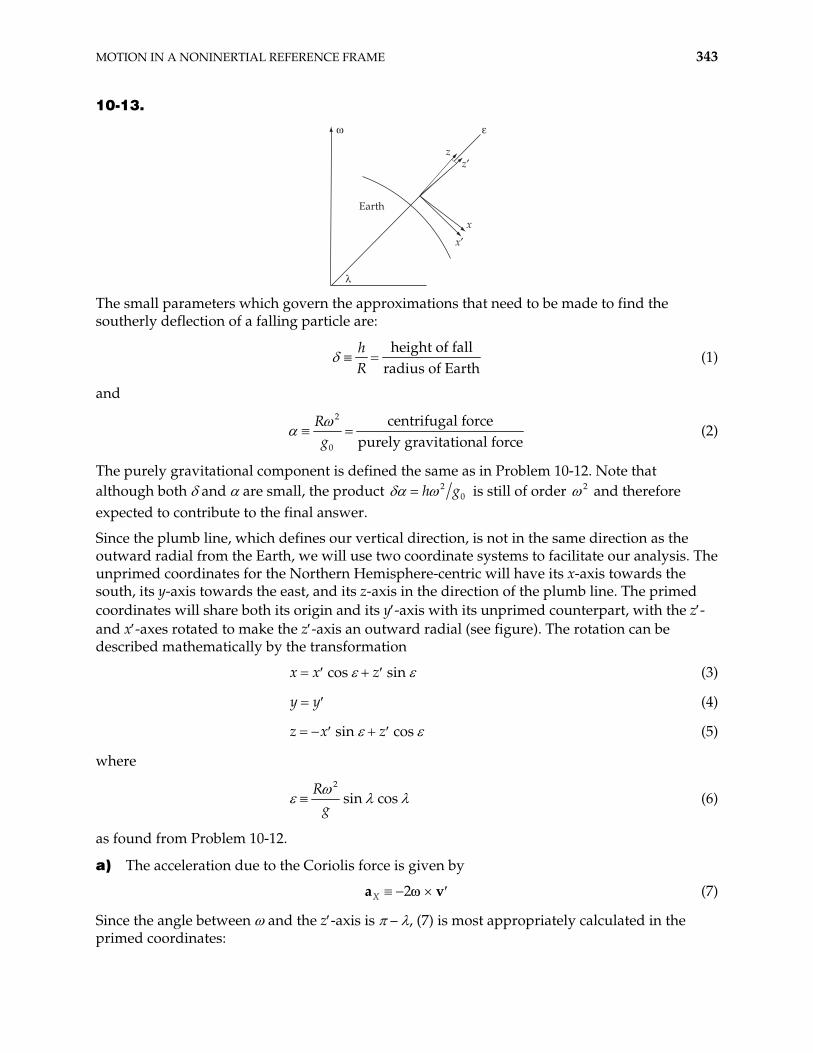
MOTION IN A NONINERTIAL REFERENCE FRAME 343
10-13.
"
$
%
z#z
x
x#
Earth
The small parameters which govern the approximations that need to be made to find the southerly deflection of a falling particle are:
height of fall
radius of EarthhR
(1)
and
2
0
centrifugal forcepurely gravitational force
Rg
(2)
The purely gravitational component is defined the same as in Problem 10-12. Note that although both and are small, the product 2
0h g is still of order 2 and therefore expected to contribute to the final answer.
Since the plumb line, which defines our vertical direction, is not in the same direction as the outward radial from the Earth, we will use two coordinate systems to facilitate our analysis. The unprimed coordinates for the Northern Hemisphere-centric will have its x-axis towards the south, its y-axis towards the east, and its z-axis in the direction of the plumb line. The primed coordinates will share both its origin and its y -axis with its unprimed counterpart, with the z - and x -axes rotated to make the z -axis an outward radial (see figure). The rotation can be described mathematically by the transformation
cos sinx x z (3)
(4) y y
sin cosz x z (5)
where
2
sin cosR
g (6)
as found from Problem 10-12.
a) The acceleration due to the Coriolis force is given by
2Xa v (7)
Since the angle between and the z -axis is – , (7) is most appropriately calculated in the primed coordinates:
344 CHAPTER 10
2 sinx y (8)
2 cos siny z x (9)
2 cosz y (10)
In the unprimed coordinates, the interesting component is
2 sin cos cos sinx y (11)
At our level approximation this becomes
2 sinx y (12)
Using the results for and y z , which is correct to order (also found from Example 10.3),
2 22 sin cosx gt (13)
Integrating twice and using the zeroth order result for the time-of-fall, 2ht , we obtain for the deflection
g
2
22sin cos
3Xh
dg
(14)
b) The centrifugal force gives us an acceleration of
ca r (15)
The component equations are then
2 sin sin cosx x R z (16)
(17) 2y y
20cos sin cosz x R z g (18)
where we have included the pure gravitational component of force as well. Now transform to the unprimed coordinates and approximate
20sin cos sinx R z g (19)
We can use Problem 10-12 to obtain sin to our level of approximation
2
0
sin sin cosRg
(20)
The prompts a cancellation in equation (19), which becomes simply
2 sin cosx z (21)
Using the zeroth order result for the height, 2 2z h gt , and for the time-of-fall estimates the deflection due to the centrifugal force
2
25sin cos
6ch
dg
(22)
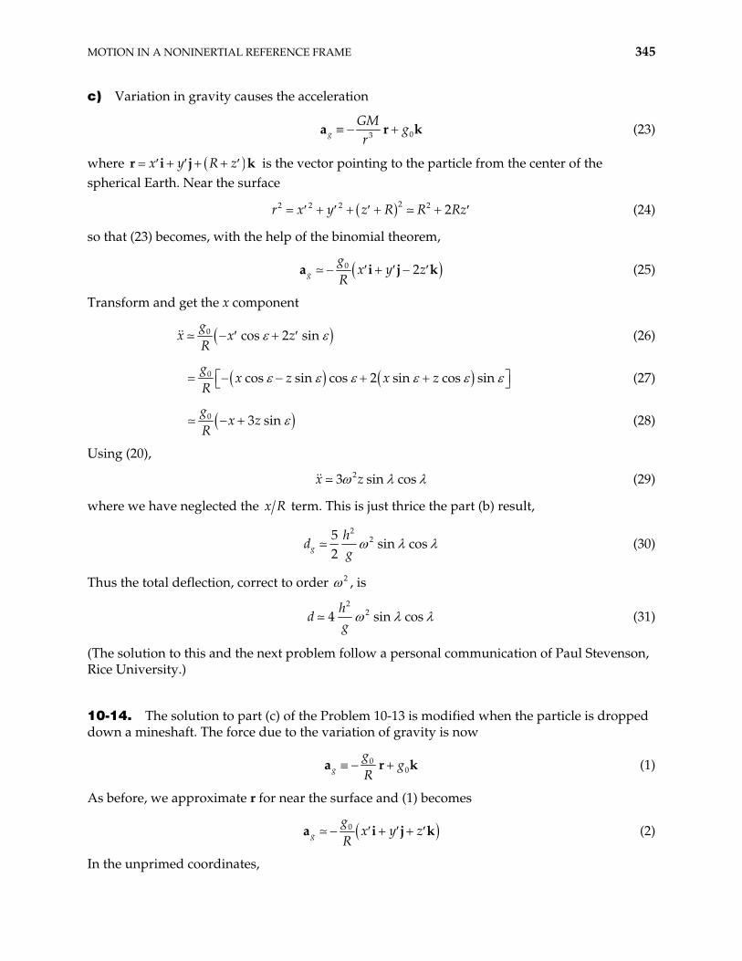
MOTION IN A NONINERTIAL REFERENCE FRAME 345
c) Variation in gravity causes the acceleration
03gGM
gr
a r k (23)
where x y R zjr i is the vector pointing to the particle from the center of the spherical Earth. Near the surface
k
22 2 2 2 2r x y z R R Rz (24)
so that (23) becomes, with the help of the binomial theorem,
0 2gg
x y zR
a i j k (25)
Transform and get the x component
0 cos 2 sing
x x zR
(26)
0 cos sin cos 2 sin cos sing
x z x zR
(27)
0 3 sing
x zR
(28)
Using (20),
23 sin cosx z (29)
where we have neglected the x term. This is just thrice the part (b) result, R
2
25sin cos
2gh
dg
(30)
Thus the total deflection, correct to order 2 , is
2
24 sin cosh
dg
(31)
(The solution to this and the next problem follow a personal communication of Paul Stevenson, Rice University.)
10-14. The solution to part (c) of the Problem 10-13 is modified when the particle is dropped down a mineshaft. The force due to the variation of gravity is now
00g
gg
Ra r k (1)
As before, we approximate r for near the surface and (1) becomes
0g
gx y z
Ra i j k (2)
In the unprimed coordinates,
346 CHAPTER 10
0x
x gR
(3)
To estimate the order of this term, as we probably should have done in part (c) of Problem 10-13, we can take 2 2~x h g , so that
2~h
x hR
(4)
which is reduced by a factor h R from the accelerations obtained previously. We therefore have no southerly deflection in this order due to the variation of gravity. The Coriolis and centrifugal forces still deflect the particle, however, so that the total deflection in this approximation is
2
23sin cos
2h
dg
(5)
10-15. The Lagrangian in the fixed frame is
212 f fL mv U r (1)
where fv and fr are the velocity and the position, respectively, in the fixed frame. Assuming we have common origins, we have the following relation
f r rv v r (2)
where v and are measured in the rotating frame. The Lagrangian becomes r rr
22 22 r r r rm
Uv r r rrL v (3)
The canonical momentum is
r rr
Lm m rp v
vr (4)
The Hamiltonian is then
221 12 2r r r r rmv U r mv p rH L (5)
H is a constant of the motion since 0L t , but H E since the coordinate transformation equations depend on time (see Section 7.9). We can identify
212cU m rr (6)
as the centrifugal potential energy because we may find, with the use of some vector identities,
22 2
2c rm
U r rr (7)
2r rm r r (8)
MOTION IN A NONINERTIAL REFERENCE FRAME 347
rm r (9)
which is the centrifugal force. Computing the derivatives of (3) required in Lagrange’s equations
rr
dm m
dt rL
av
v (10)
r r cr
mL
v rr
U U (11)
r rm m Uv r (12)
The equation of motion we obtain is then
2r rm ma r rv
a
m U (13)
If we identify F and F , then we do indeed reproduce the equations of motion given in Equation 10.25, without the second and third terms.
eff rm U
10-16. The details of the forces involved, save the Coriolis force, and numerical integrations in the solution of this problem are best explained in the solution to Problem 9-63. The only thing we do here is add an acceleration caused by the Coriolis force, and re-work every part of the problem over again. This is conceptually simple but in practice makes the computation three times more difficult, since we now also must include the transverse coordinates in our integrations. The acceleration we add is
2 sin sin cos cosc y x z yv v v vj ka i (1)
where we have chosen the usual coordinates as shown in Figure 10-9 of the text.
a) Our acceleration is
Cga k a (2)
As a check, we find that the height reached is 1800 km, in good agreement with the result of
Problem 9-63(a). The deflection at this height is found to be 77 km, to the west.
b) This is mildly tricky. The correct treatment says that the equation of motion with air resistance is (cf. equation (2) of Problem 9-63 solution)
2 Ct
vg
va k v a (3)
The deflection is calculated to be 8.9 km.
c) Adding the vaiation due to gravity gives us a deflection of 10 km.
d) Adding the variation of air density gives us a deflection of 160 km.
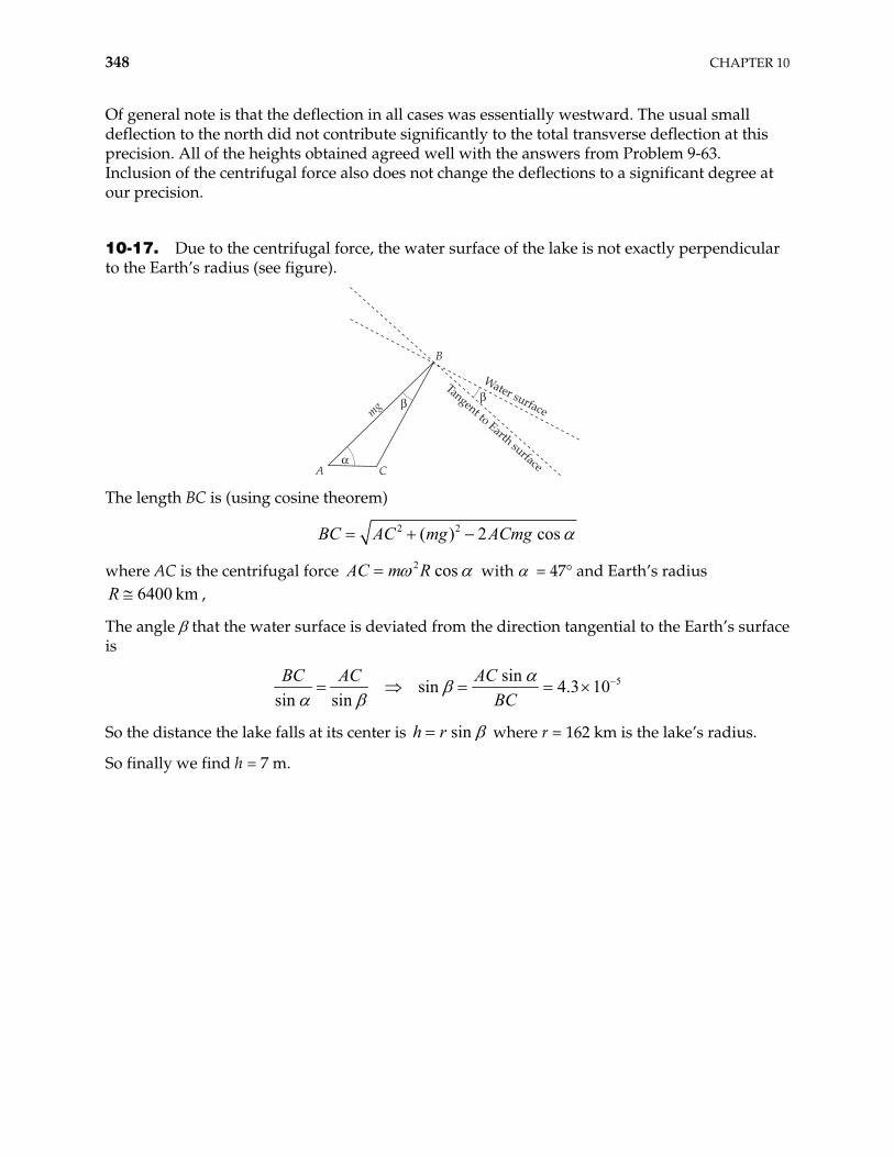
348 CHAPTER 10
Of general note is that the deflection in all cases was essentially westward. The usual small deflection to the north did not contribute significantly to the total transverse deflection at this precision. All of the heights obtained agreed well with the answers from Problem 9-63. Inclusion of the centrifugal force also does not change the deflections to a significant degree at our precision.
10-17. Due to the centrifugal force, the water surface of the lake is not exactly perpendicular to the Earth’s radius (see figure).
mg
C
B
& &Water surface
Tangent to Earth surface'A
The length BC is (using cosine theorem)
2 2( ) 2 cosAC mg ACmgBC
where AC is the centrifugal force 2 cosAC m R with = 47° and Earth’s radius , 6400 kmR
The angle that the water surface is deviated from the direction tangential to the Earth’s surface is
5sinsin 4.3 10
sin sin
BC AC ACBC
So the distance the lake falls at its center is sinh r where r = 162 km is the lake’s radius.
So finally we find h = 7 m.
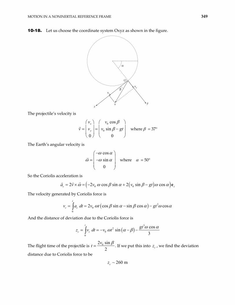
MOTION IN A NONINERTIAL REFERENCE FRAME 349
10-18. Let us choose the coordinate system Oxyz as shown in the figure.
O
(x
(y
(
&
'
xy
The projectile’s velocity is
v v where = 37° 0
0
cossin
0 0
x
y
v vv gt
The Earth’s angular velocity is
cossin0
where = 50°
So the Coriolis acceleration is
0 02 2 cos sin 2 sin cosc zv v gt ea v
The velocity generated by Coriolis force is
20
0
2 cos sin sin cos cost
c ca dt v t gtv
And the distance of deviation due to the Coriolis force is
3
20
0
cossin
3
t
c cgt
dt v tz v
The flight time of the projectile is 02 sin2
vt . If we put this into , we find the deviation
distance due to Coriolis force to be
cz
~ 260 mcz
350 CHAPTER 10
10-19. The Coriolis force acting on the car is
2 2 sinc cF m v F mv
where = 65°, m = 1300 kg, v = 100 km/hr.
So 4.76 N.cF
10-20. Given the Earth’s mass, M , the magnitude of the gravitational field vector at the poles is
245.976 10 kg
22 9.866 m/spolepole
GMg
R
The magnitude of the gravitational field vector at the equator is
2 2e2 R 9.768 m/seq q
eq
GMg
R
where is the angular velocity of the Earth about itself.
If one use the book’s formula, we have
at the poles 2( 90 ) 9.832 m/sg
and
g at the equator 2( 0 ) 9.780 m/s
10-21. The Coriolis acceleration acting on flowing water is
2 2 sinc ca v a v
Due to this force, the water is higher on the west bank. As in problem 10-17, the angle that the water surface is deviated from the direction tangential to Earth’s surface is
5
2 2 2 2 2 2
2 sin2.5 10
4 sinsin c
c
a v
g a g v
The difference in heights of the two banks is
3sin 1.2 10 mh
where m is the river’s width. 47
10-22. The Coriolis acceleration is 2ca v . This acceleration ca pushes lead bullets
eastward with the magnitude 2 coscos 2c gta v , where = 42°.
The velocity generated by the Coriolis force is
MOTION IN A NONINERTIAL REFERENCE FRAME 351
2( ) coscv t a dt gt
and the deviation distance is
3
( ) cos3c c
gtx v t dt
The falling time of the bullet is 2ht . So finally g
3
38cos 2.26 10 m
3c
hx
g

352 CHAPTER 10
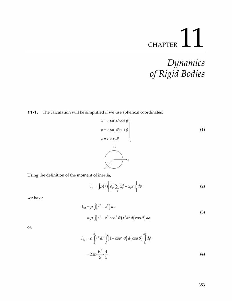
CHAPTER 11 Dynamics
of Rigid Bodies
11-1. The calculation will be simplified if we use spherical coordinates:
sin cos
sin sin
cos
x r
y r
z r
(1)
z
y
x Using the definition of the moment of inertia,
2ij ij k i j
k
I r x x x dv (2)
we have
2 233
2 2 2 2cos cos
I r z dv
r r r dr d d (3)
or,
1 24 2
330 1 0
5
1 cos cos
42
5 3
R
I r dr d
R
d
(4)
353
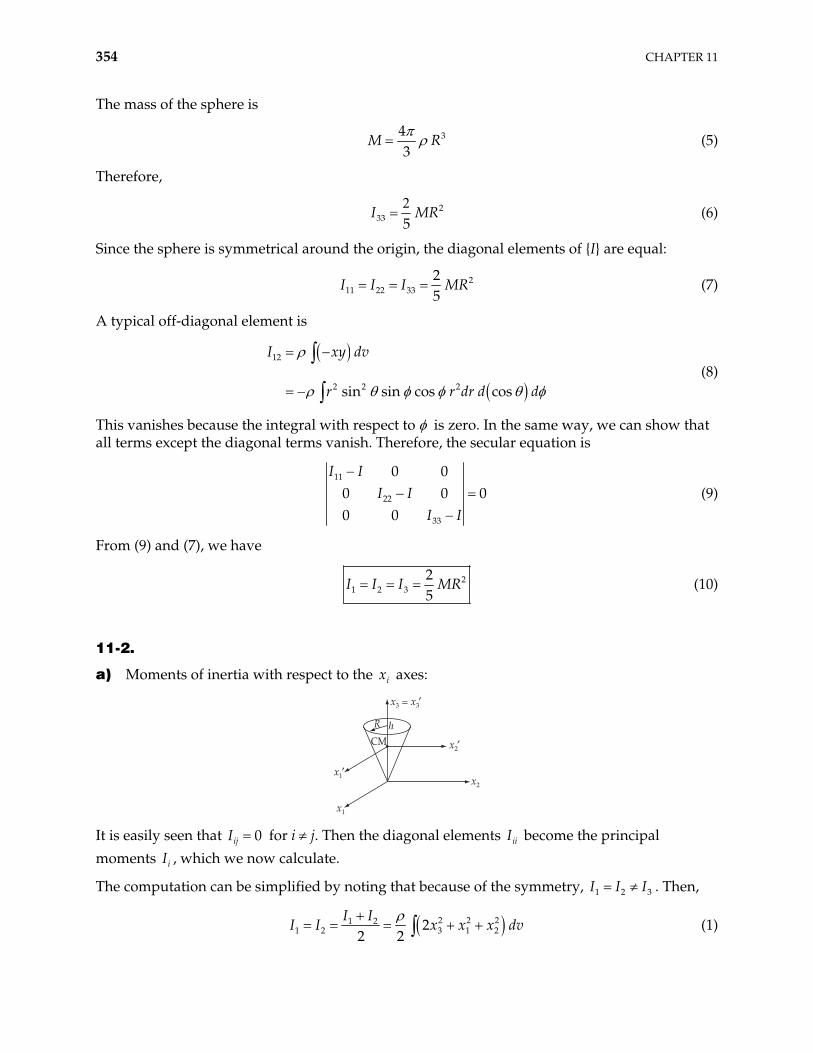
354 CHAPTER 11
The mass of the sphere is
343
M R (5)
Therefore,
233 5
I MR (6)
Since the sphere is symmetrical around the origin, the diagonal elements of {I} are equal:
211 22 33
25
I I I MR (7)
A typical off-diagonal element is
12
2 2 2sin sin cos cos
I xy dv
r r dr d d (8)
This vanishes because the integral with respect to is zero. In the same way, we can show that all terms except the diagonal terms vanish. Therefore, the secular equation is
11
22
33
0 00 00 0
I II I
I I0 (9)
From (9) and (7), we have
21 2 3
25
I I I MR (10)
11-2.
a) Moments of inertia with respect to the x axes: i
x3 = x3!
R hCM
x1
x1! x2
x2!
It is easily seen that for i j. Then the diagonal elements become the principal moments I , which we now calculate.
0ijI iiI
i
The computation can be simplified by noting that because of the symmetry, . Then, 1 2I I I3
2 2 21 21 2 3 1 22
2 2I I
x x x dI I v (1)
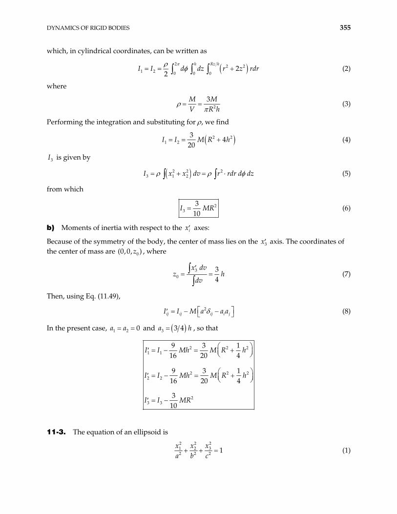
DYNAMICS OF RIGID BODIES 355
which, in cylindrical coordinates, can be written as
2 2 2
1 2 0 0 02
2h Rz h
d dz r z rdI I r (2)
where
2
3M MV R h
(3)
Performing the integration and substituting for , we find
21 2
34
20I I M R h2 (4)
3I is given by
2 2 23 1 2I x x dv r rdr d dz (5)
from which
23
310
I MR (6)
b) Moments of inertia with respect to the xi axes:
Because of the symmetry of the body, the center of mass lies on the 3x axis. The coordinates of the center of mass are (0 0,0, )z , where
3
034
x dvz h
dv (7)
Then, using Eq. (11.49),
2ij ij ij i jI I M a a a (8)
In the present case, and 1 2 0a a 3 3 4a h , so that
2 21 1
2 22 2
23 3
9 3 116 20 4
9 3 116 20 4
310
I I Mh M R h
I I Mh M R h
I I MR
2
2
11-3. The equation of an ellipsoid is
22 231 2
2 2 2 1xx x
a b c (1)
356 CHAPTER 11
which can be written in normalized form if we make the following substitutions:
1 2 3, ,x a x b x c (2)
Then, Eq. (1) reduces to
2 2 2 1 (3)
This is the equation of a sphere in the ( , , ) system.
If we denote by dv the volume element in the system and by d the volume element in the ( , , ) system, we notice that the volume of the ellipsoid is
ix
1 2 3
43
V dv dx dx dx abc d d d
abc d abc (4)
because d is just the volume of a sphere of unit radius.
The rotational inertia with respect to the passing through the center of mass of the ellipsoid (we assume the ellipsoid to be homogeneous), is given by
3 -axisx
2 23 1 2
2 22 2
MI x x dv
V
Mabc a b d
V (5)
In order to evaluate this integral, consider the following equivalent integral in which z = r cos :
2 2 2 2
2 12 2
0 0 0
2
2
sin
cos sin
2 12
3 5
415
R
a z dv a z r dr r d d
a d d r d
a
a
4 r
(6)
Therefore,
2 22 2 2415
a b d a b2 (7)
and
2 23
15
I M a b (8)
Since the same analysis can be applied for any axis, the other moments of inertia are
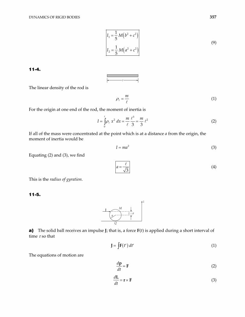
DYNAMICS OF RIGID BODIES 357
2 21
2 22
15
15
I M b c
I M a c
(9)
11-4.
The linear density of the rod is
m
(1)
For the origin at one end of the rod, the moment of inertia is
3
2
0 3 3m m
I x dx 2 (2)
If all of the mass were concentrated at the point which is at a distance a from the origin, the moment of inertia would be
(3) 2I ma
Equating (2) and (3), we find
3
a (4)
This is the radius of gyration.
11-5.
J M
a
Q
z – a
z
a) The solid ball receives an impulse J; that is, a force F(t) is applied during a short interval of time so that
t dtJ F (1)
The equations of motion are
ddtp
F (2)
ddtL
r F (3)
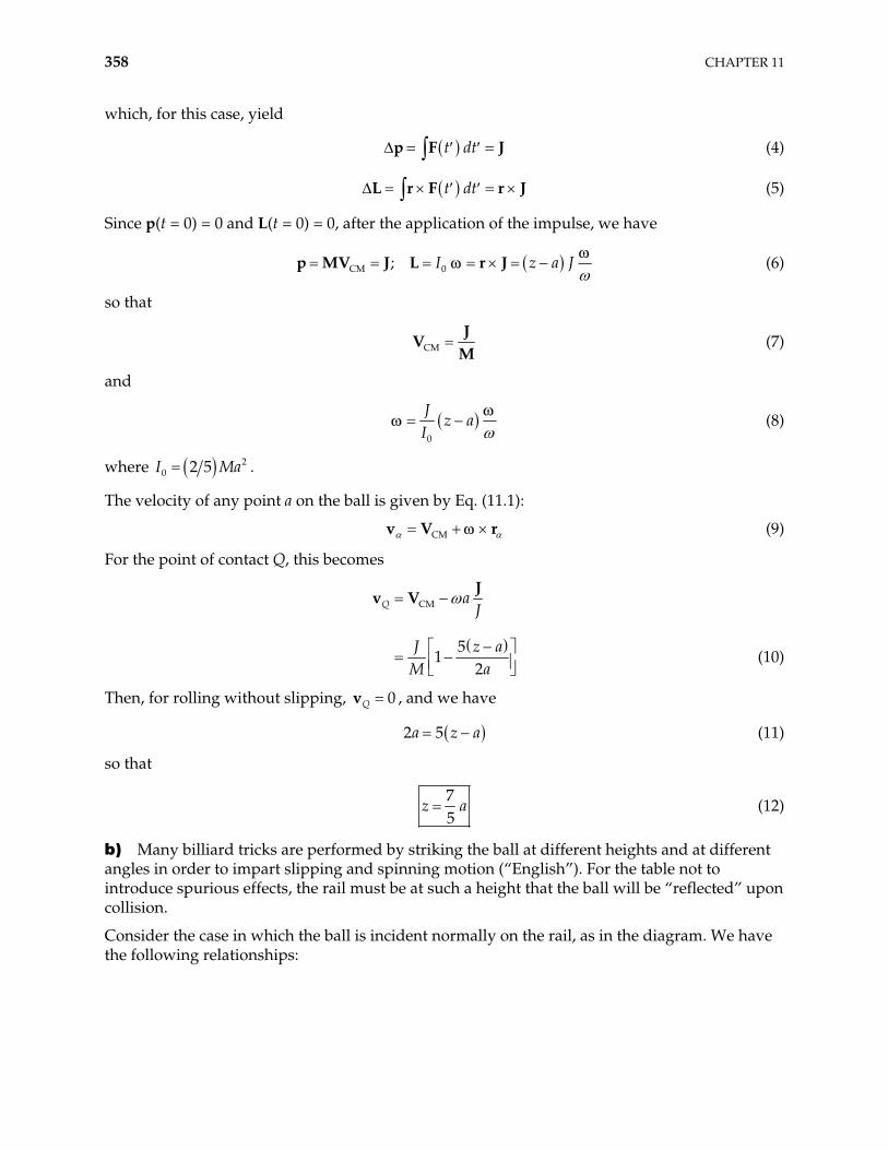
358 CHAPTER 11
which, for this case, yield
t dtp F J (4)
t dtL r F r J (5)
Since p(t = 0) = 0 and L(t = 0) = 0, after the application of the impulse, we have
CM 0; I z a JV J L r Jp M (6)
so that
CMJ
VM
(7)
and
0
Jz a
I (8)
where 20 2 5I Ma .
The velocity of any point a on the ball is given by Eq. (11.1):
CMv V r (9)
For the point of contact Q, this becomes
CM
51
2
Q aJ
J z aM a
Jv V
(10)
Then, for rolling without slipping, 0Qv , and we have
2 5a z a (11)
so that
75
z a (12)
b) Many billiard tricks are performed by striking the ball at different heights and at different angles in order to impart slipping and spinning motion (“English”). For the table not to introduce spurious effects, the rail must be at such a height that the ball will be “reflected” upon collision.
Consider the case in which the ball is incident normally on the rail, as in the diagram. We have the following relationships:
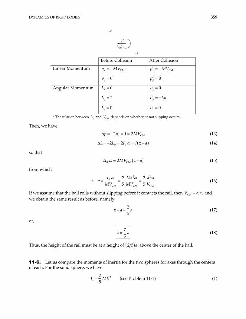
DYNAMICS OF RIGID BODIES 359
y
x
VCM
Before Collision After Collision
Linear Momentum CM
0
x
y
p MV
p
CM
0
x
y
p MV
p
Angular Momentum 0
*
0
x
y
z
L
L
L
0
0
x
y
z
L
L L
L
y
* The relation between and depends on whether or not slipping occurs. yL CMV
Then, we have
CM2 2xp p J MV (13)
02 2yL L I J z a (14)
so that
0 CM2 2I MV z a (15)
from which
2 2
0
CM CM CM
2 25 5
I Ma az a
MV MV V (16)
If we assume that the ball rolls without slipping before it contacts the rail, then VCM a , and we obtain the same result as before, namely,
25
z a a (17)
or,
75
z a (18)
Thus, the height of the rail must be at a height of 2 5 a above the center of the ball.
11-6. Let us compare the moments of inertia for the two spheres for axes through the centers of each. For the solid sphere, we have
22(see Problem 11-1)
5sI MR (1)
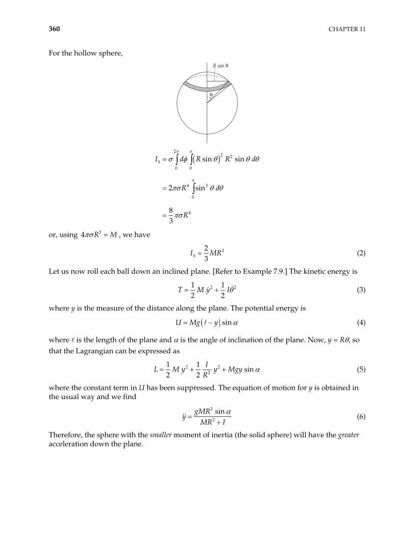
360 CHAPTER 11
For the hollow sphere,
"
R sin "
22 2
0 0
4 3
0
4
sin sin
2 sin
83
hI d R R
R d
R
d
or, using , we have 24 R M
223hI MR (2)
Let us now roll each ball down an inclined plane. [Refer to Example 7.9.] The kinetic energy is
21 12 2
T M y I 2 (3)
where y is the measure of the distance along the plane. The potential energy is
sinU Mg y (4)
where is the length of the plane and is the angle of inclination of the plane. Now, y = R , so that the Lagrangian can be expressed as
2 22
1 1sin
2 2I
L M y y MgyR
(5)
where the constant term in U has been suppressed. The equation of motion for y is obtained in the usual way and we find
2
2
singMRy
MR I (6)
Therefore, the sphere with the smaller moment of inertia (the solid sphere) will have the greater acceleration down the plane.
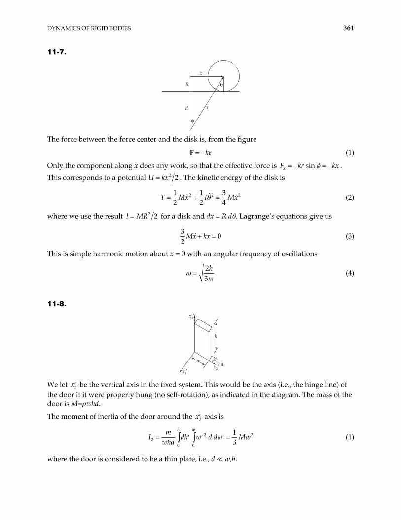
DYNAMICS OF RIGID BODIES 361
11-7.
R
d
x
r
#
"
The force between the force center and the disk is, from the figure
kF r (1)
Only the component along x does any work, so that the effective force is sinxF kr kx .
This corresponds to a potential 2 2xU k . The kinetic energy of the disk is
2 21 1 32 2 4
T Mx I Mx2 (2)
where we use the result 2 2I MR for a disk and dx = R d . Lagrange’s equations give us
3
02
Mx kx (3)
This is simple harmonic motion about x = 0 with an angular frequency of oscillations
23
km
(4)
11-8.
x3!
x1!x2!
d
h
w
We let be the vertical axis in the fixed system. This would be the axis (i.e., the hinge line) of the door if it were properly hung (no self-rotation), as indicated in the diagram. The mass of the door is M= whd.
3x
The moment of inertia of the door around the x3 axis is
23
0 0
13
h wmI dh w d dw
whd2Mw (1)
where the door is considered to be a thin plate, i.e., d w,h.
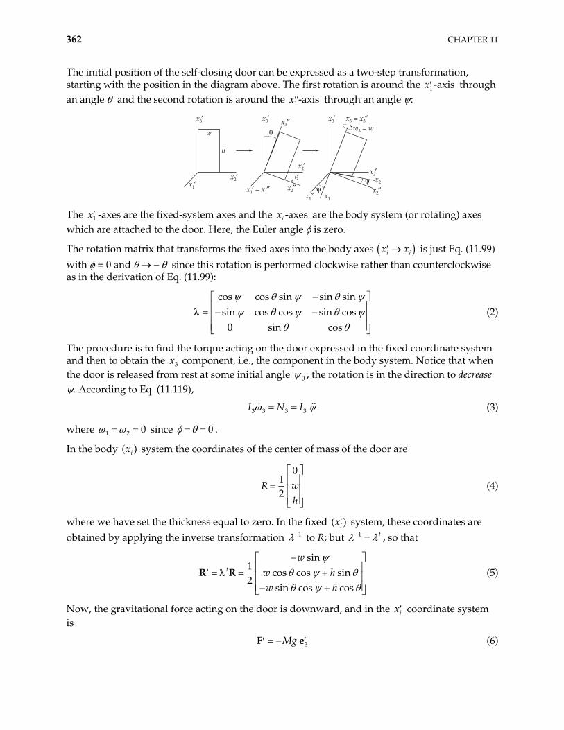
362 CHAPTER 11
The initial position of the self-closing door can be expressed as a two-step transformation, starting with the position in the diagram above. The first rotation is around the through an angle and the second rotation is around the
1 -axisx
1 -axisx through an angle :
w
h
x3!
x2!x1!
x3! x3$
x2!
x2$x1! = x1$
"
"
x3! x3 = x3$w3 = w
x2!x2
x2$x1$ x1
%%
The -axes are the fixed-system axes and the are the body system (or rotating) axes which are attached to the door. Here, the Euler angle is zero.
1x -axesix
The rotation matrix that transforms the fixed axes into the body axes ix xi is just Eq. (11.99) with = 0 and – since this rotation is performed clockwise rather than counterclockwise as in the derivation of Eq. (11.99):
cos cos sin sin sinsin cos cos sin cos
0 sin cos (2)
The procedure is to find the torque acting on the door expressed in the fixed coordinate system and then to obtain the component, i.e., the component in the body system. Notice that when the door is released from rest at some initial angle
3x
0 , the rotation is in the direction to decrease . According to Eq. (11.119),
3 3 3 3I N I (3)
where 1 2 0 since . 0
In the body ( system the coordinates of the center of mass of the door are )ix
0
12
R wh
(4)
where we have set the thickness equal to zero. In the fixed ( )ix system, these coordinates are obtained by applying the inverse transformation 1 to R; but 1 t , so that
sin
1cos cos sin
2sin cos cos
t
ww hw h
R R (5)
Now, the gravitational force acting on the door is downward, and in the coordinate system is
ix
3MgF e (6)
DYNAMICS OF RIGID BODIES 363
There the torque on the door, expressed in the fixed system, is
1 2 31sin cos cos sin sin cos cos
20 0 1
cos cos sin1
sin2
0
Mg w w h w h
w hMg w
N R F
e e e
(7)
so that in the body system we have
2 2cos cos sin cos cos sin1
sin sin2
sin sin
w h wMg h
wN N (8)
Thus,
31
sin sin2
N Mgw (9)
and substituting this expression into Eq. (3), we have
23
1 1sin sin
2 3Mgw I Mw (10)
where we have used Eq. (1) for . Solving for 3I ,
3
sin sin2
gw
(11)
This equation can be integrated by first multiplying by :
21 3sin sin
2 2
3sin cos
2
gdt dt
w
gw
(12)
where the integration constant is zero since cos 0 when 0 . Thus,
3
sin cosg
w (13)
We must choose the negative sign for the radical since 0 when cos 0 . Integrating again, from = 90° to = 0°,
0
02
3sin
cos
Tgddt
w (14)
364 CHAPTER 11
where T = 2 sec. Rewriting Eq. (14),
2
0
3sin
cosgd
Tw
(15)
Using Eq. (E. 27a), Appendix E, we find
2
1 2
0
14cos324
d (16)
From Eqs. (E.20) and (E.23),
1 1 11 0.906
4 4 4
13.624
4 (17)
And from Eqs. (E.20) and (E.24),
3 3 31 0.919
4 4 4
31.225
4 (18)
Therefore,
2
0
3.6242.62
2 1.225cosd
(19)
Returning to Eq. (15) and solving for sin ,
22sin 2.62
3wgT
(20)
Inserting the values for g, w(= 1m), and T(= 2 sec), we find
1sin 0.058
or,
3.33 (21)
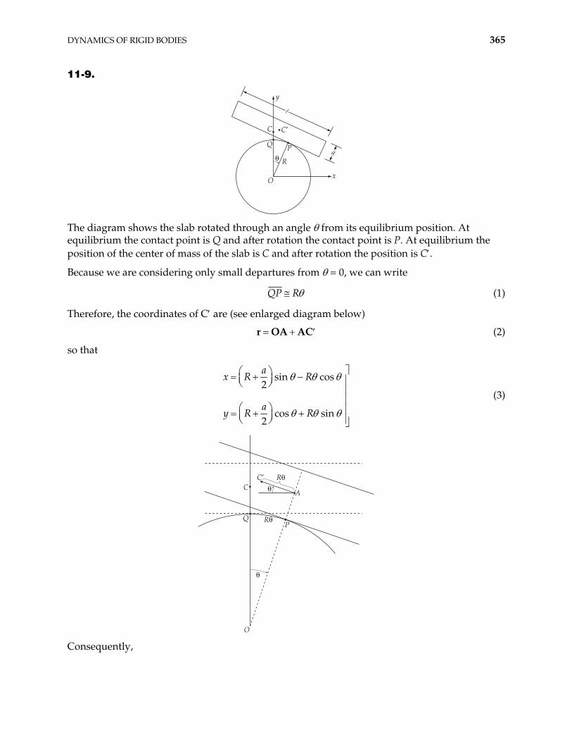
DYNAMICS OF RIGID BODIES 365
11-9.
a
O
R
Q P
C C!
"
y
x
The diagram shows the slab rotated through an angle from its equilibrium position. At equilibrium the contact point is Q and after rotation the contact point is P. At equilibrium the position of the center of mass of the slab is C and after rotation the position is C .
Because we are considering only small departures from = 0, we can write
QP R (1)
Therefore, the coordinates of C are (see enlarged diagram below)
r OA AC (2)
so that
sin cos2
cos sin2
ax R R
ay R R
(3)
C
Q
C!
R"
R"
P
O
A
"
"
Consequently,
366 CHAPTER 11
cos cos sin2
cos sin2
sin cos sin2
sin cos2
ax R R R
aR
ay R R R
aR
from which
2
2 2 2 2
4a
x y R 2 (4)
The kinetic energy is
2 21 12 2
T M x y I 2 (5)
where I is the moment of inertia of the slab with respect to an axis passing through the center of mass and parallel to the z-axis:
2 2112
I M a (6)
Therefore,
21
12
T f (7)
where
2
2 21 4
af M R I (8)
The potential energy is
2U Mgy f (9)
where
2 cos sin2a
f Mg R R (10)
and where Eq. (3) has been used for y.
The Lagrangian is
21
12
L f f2 (11)
The Lagrange equation for is
DYNAMICS OF RIGID BODIES 367
0d L Ldt
(12)
Now,
1L
f
1 1
22 2 2 22
4
d Lf f
dt
aM R I MR (13)
21 2
2 2
12
sin cos sin2
Lf f
aMR Mg R R R (14)
Combining, we find
22 2 2 2 sin cos sin 0
4 2a a
M R I MR Mg R R R (15)
For the case of small oscillations, 2 and 2 , so that Eq. (15) reduces to
22 0
4
aMg R
MaI
(16)
The system is stable for oscillations around = 0 only if
22
2 0
4
aMg R
MaI
(17)
This condition is satisfied if 2 0R a , i.e.,
2a
R (18)
Then, the frequency is
22 2
21
4 12
aMg R
Ma M a (19)
Simplifying, we have
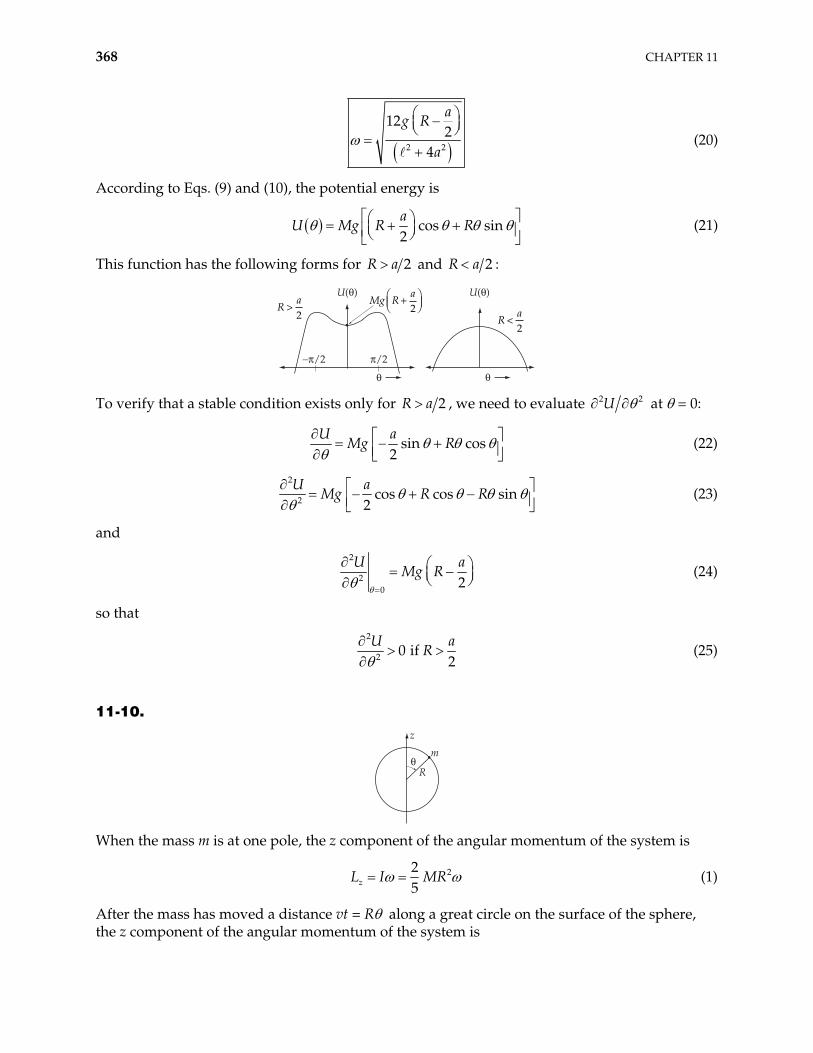
368 CHAPTER 11
2 2
122
4
ag R
a (20)
According to Eqs. (9) and (10), the potential energy is
cos sin2a
U Mg R R (21)
This function has the following forms for 2R a and 2R a :
U(") U(")
"
&'/2 '/2
Ra>2 R
a<2
Mg Ra+(
)*+,-2
"
To verify that a stable condition exists only for 2R a , we need to evaluate 2U 2 at = 0:
sin cos2
U aMg R (22)
2
2 cos cos sin2
U aMg R R (23)
and
2
20 2
UMg R
a (24)
so that
2
2 0 if 2
UR
a (25)
11-10.
z
m
R"
When the mass m is at one pole, the z component of the angular momentum of the system is
225zL I MR (1)
After the mass has moved a distance vt = R along a great circle on the surface of the sphere, the z component of the angular momentum of the system is
DYNAMICS OF RIGID BODIES 369
2 2 22sin
5zL MR mR (2)
where is the new angular velocity. Since there is no external force acting on the system, angular momentum must be conserved. Therefore, equating (1) and (2), we have
2
2 2 2
25
2 sin5
MR
MR mR (3)
Substituting vt R and integrating over the time interval during which the mass travels from one pole to the other, we have
2
2 2 20
25
2 sin5
Rt
V
t
MRdt
MR mR vt R (4)
Making the substitutions,
,vt R u dt R v du (5)
we can rewrite (4) as
2
2 2 20
2
20
25
2 sin5
21 sin
MR Rdu
vMR mR u
R duv u
(6)
where 5 2m M and where we have used the fact that the integrand is symmetric around 2u to write as twice the value of the integral over half the range. Using the identity
2 1sin 1 cos 2
2u u (7)
we express (6) as
2
0
21 11 c2 2
R duv uos 2
(8)
or, changing the variable to x = 2u,
0 1 11 c
2 2
R dxv xos
(9)
Now, we can use Eq. (E.15), Appendix E, to obtain
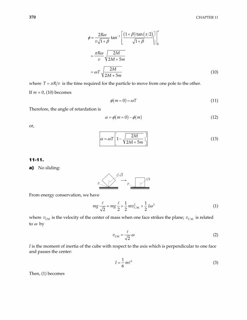
370 CHAPTER 11
1
0
1 tan 22tan
1 1
22 5
22 5
xRv
R Mv M m
MT
M m (10)
where T R v is the time required for the particle to move from one pole to the other.
If m = 0, (10) becomes
0m T (11)
Therefore, the angle of retardation is
0m m (12)
or,
2
12 5
MT
M m (13)
11-11.
a) No sliding:
PP
22
From energy conservation, we have
2C.M.
1 12 2 22
mg mg mv I 2 (1)
where v is the velocity of the center of mass when one face strikes the plane; v is related to by
CM C.M.
CM 2v (2)
I is the moment of inertia of the cube with respect to the axis which is perpendicular to one face and passes the center:
216
I m (3)
Then, (1) becomes
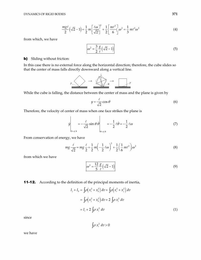
DYNAMICS OF RIGID BODIES 371
2 2
2 21 1 12 1
2 2 2 6 32mg m
m 2m (4)
from which, we have
2 32 1
2g
(5)
b) Sliding without friction:
In this case there is no external force along the horizontal direction; therefore, the cube slides so that the center of mass falls directly downward along a vertical line.
P"P
While the cube is falling, the distance between the center of mass and the plane is given by
cos2
y (6)
Therefore, the velocity of center of mass when one face strikes the plane is
0 4 4
1 1sin
2 22y (7)
From conservation of energy, we have
2
21 1 1 12 2 2 2 62
mg m m 2mg (8)
from which we have
2 122 1
5g
(9)
11-12. According to the definition of the principal moments of inertia,
2 2 2 2
2 2 2
2
2
2
j k i k i j
j k i
i i
I I x x dv x x dv
x x dv x dv
I x dv (1)
since
2 0ix dv
we have
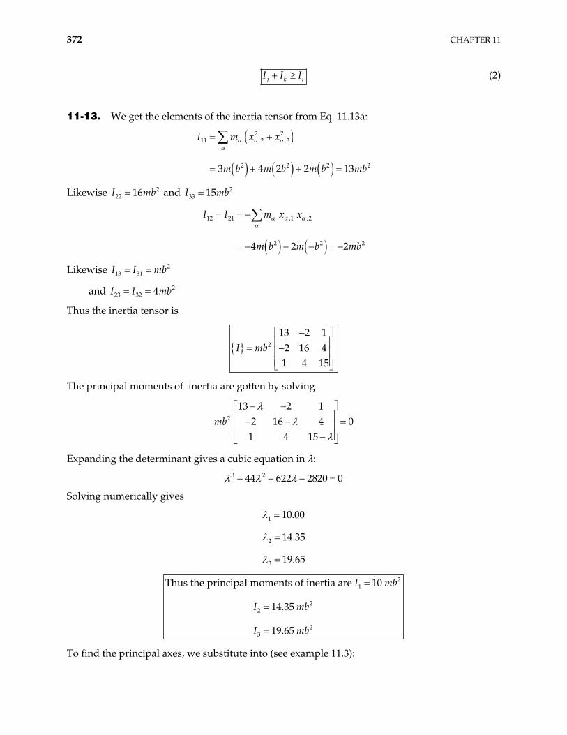
372 CHAPTER 11
j k iI I I (2)
11-13. We get the elements of the inertia tensor from Eq. 11.13a:
2 211 ,2 ,3
2 2 23 4 2 2 13
I m x x
m b m b m b mb2
b b
2
Likewise and 222 16I m 2
33 15I m
12 21 ,1 ,2
2 24 2 2
I I m x x
m b m b mb
Likewise 213 31I I mb
and I I 223 32 4mb
Thus the inertia tensor is
2
13 2 12 16 4
1 4 15I mb
The principal moments of inertia are gotten by solving
2
13 2 12 16 4
1 4 15mb 0
Expanding the determinant gives a cubic equation in :
3 244 622 2820 0
Solving numerically gives
1
2
3
10.00
14.35
19.65
21
22
23
Thus the principal moments of inertia are 10
14.35
19.65
I mb
I mb
I mb
To find the principal axes, we substitute into (see example 11.3):
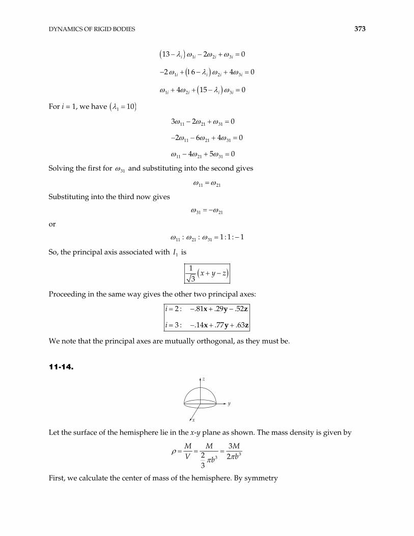
DYNAMICS OF RIGID BODIES 373
1 2 3
1 2
1 2 3
13 2 0
2 6 4
4 15 0
i i i i
i i i i
i i i i
3 0
For i = 1, we have 1 10
11 21 31
11 21 31
11 21 31
3 2 0
2 6 4
4 5 0
0
Solving the first for 31 and substituting into the second gives
11 21
Substituting into the third now gives
31 21
or
11 21 31: : 1 : 1 : 1
So, the principal axis associated with is 1I
13
x y z
Proceeding in the same way gives the other two principal axes:
2 : .81 .29 .52
3 : .14 .77 .63
i
i
x y
x y
z
z
We note that the principal axes are mutually orthogonal, as they must be.
11-14.
z
y
x Let the surface of the hemisphere lie in the x-y plane as shown. The mass density is given by
33
32 23
M M MV bb
First, we calculate the center of mass of the hemisphere. By symmetry
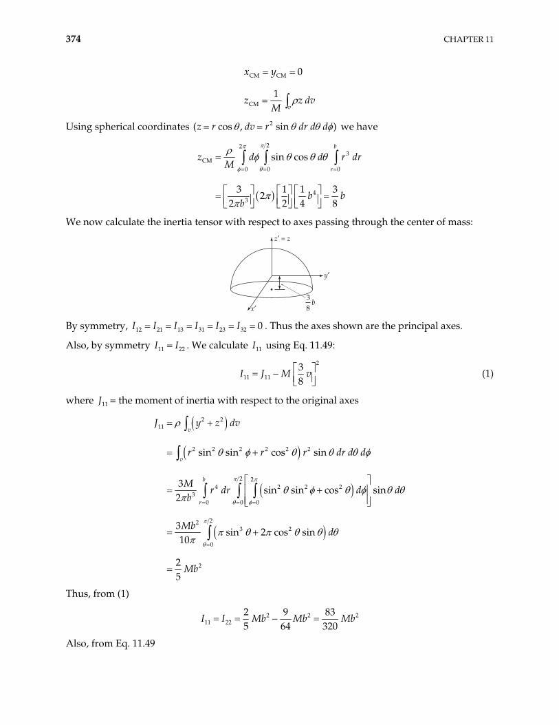
374 CHAPTER 11
CM CM
CM
0
1v
x y
z z dvM
Using spherical coordinates 2( cos , sin )z r dv r dr d d we have
223
CM0 0 0
43
sin cos
3 1 1 32
2 2 4 8
b
r
z d dM
b bb
r dr
We now calculate the inertia tensor with respect to axes passing through the center of mass:
z! = z
x!
y!
38
b
By symmetry, . Thus the axes shown are the principal axes. 12 21 13 31 23 32 0I I I I I I
Also, by symmetry I . We calculate I using Eq. 11.49: 11 22I 11
2
11 1138
I J M v (1)
where 11J = the moment of inertia with respect to the original axes
2 211
2 2 2 2 2 2
2 24 2 2 2
30 0 0
223 2
0
2
sin sin cos sin
3sin sin cos sin
2
3sin 2 cos sin
10
25
v
v
b
r
J y z dv
r r r dr d d
Mr dr d d
b
Mbd
Mb
Thus, from (1)
2 211 22
2 9 835 64 320
I I Mb Mb Mb2
Also, from Eq. 11.49
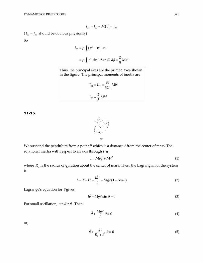
DYNAMICS OF RIGID BODIES 375
33 33 330I J M J
( should be obvious physically) 33 33I J
So
2 233
4 3 2sin
5
v
v
I x y dv
r dr d d M 2b
211 22
233
Thus, the principal axes are the primed axes shown in the figure. The principal moments of inertia are
83I
320
2I
5
I Mb
Mb
11-15.
"
P
g
We suspend the pendulum from a point P which is a distance from the center of mass. The rotational inertia with respect to an axis through P is
(1) 20I MR M 2
where is the radius of gyration about the center of mass. Then, the Lagrangian of the system is
0R
2
1 cos2
IL T U Mg (2)
Lagrange’s equation for gives
sin 0I Mg (3)
For small oscillation, sin . Then,
0Mg
I (4)
or,
2 20
0g
R (5)
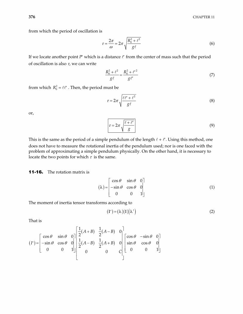
376 CHAPTER 11
from which the period of oscillation is
2 202
2R
g (6)
If we locate another point P which is a distance from the center of mass such that the period of oscillation is also , we can write
2 2 20 0R Rg g
2
(7)
from which . Then, the period must be 20R
2
2g
(8)
or,
2g
(9)
This is the same as the period of a simple pendulum of the length +
1
. Using this method, one does not have to measure the rotational inertia of the pendulum used; nor is one faced with the problem of approximating a simple pendulum physically. On the other hand, it is necessary to locate the two points for which is the same.
11-16. The rotation matrix is
cos sin 0sin cos 00 0
(1)
The moment of inertia tensor transforms according to
t (2)
That is
1 10
2 2cos sin 0 cos sin 01 1
sin cos 0 0 sin cos 02 2
0 0 1 0 00 0
A B A B
I A B A B
C 1
DYNAMICS OF RIGID BODIES 377
1 1 1 1cos sin sin cos 0
2 2 2 2cos sin 01 1 1 1
sin cos 0 cos sin sin cos 02 2 2 2
0 0 1 0 0
A B A B A B A B
A B A B A B A B
C
2 2
2 2
2 2
2 2
1 1cos cos sin sin
2 21 1
sin cos2 2
0
1 1cos sin 0
2 21 1
sin sin cos cos 02 2
0
A B A B A B
A B A B
A B A B
A B A B A B
C
or
2 2
2 2
1 1 1cos sin cos sin 0
2 2 21 1 1
sin cos cos sin 02 2 2
0 0
A B A B A B A B
A B A B A B A B
C
I (3)
If 4 , sin cos 1 2 . Then,
0 0
0 00 0
AB
CI (4)
11-17.
x3
x2
x1
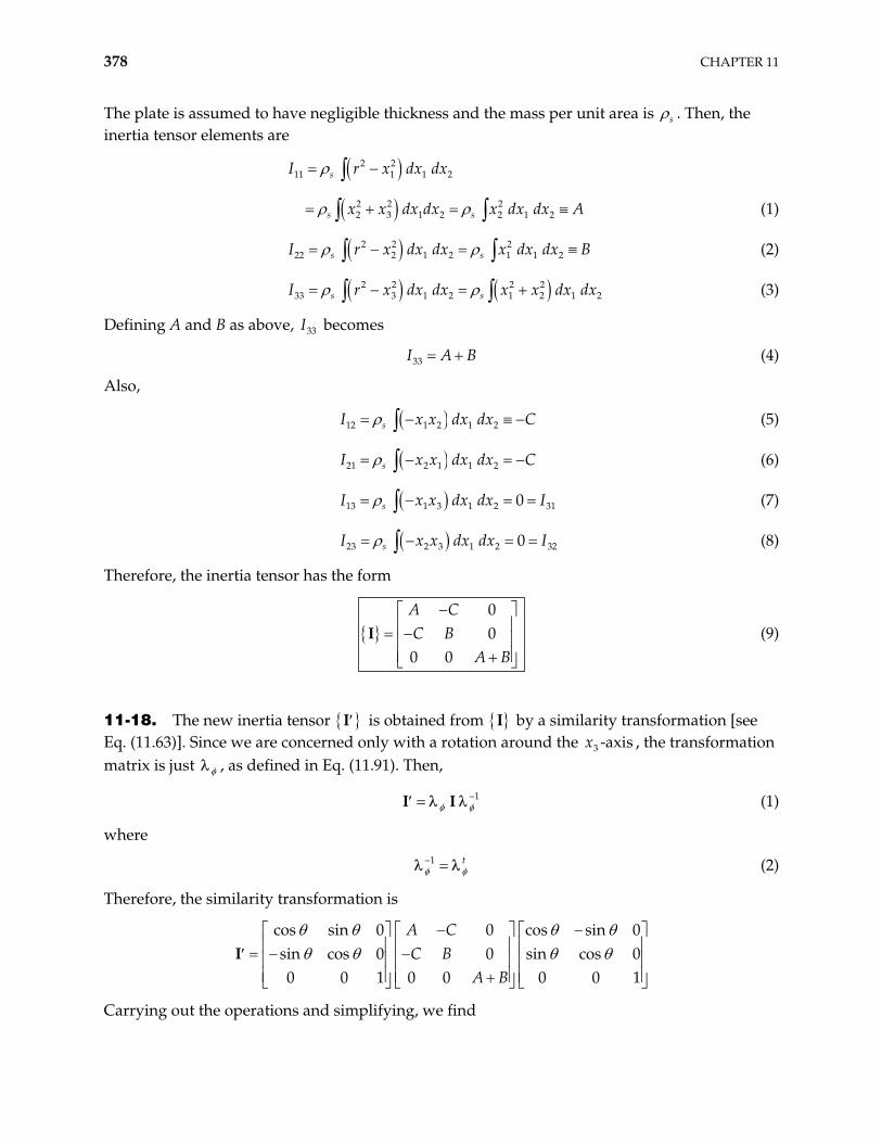
378 CHAPTER 11
The plate is assumed to have negligible thickness and the mass per unit area is s . Then, the inertia tensor elements are
2 211 1 1 2s x dxI r dx
2 2 22 3 1 2 2 1 2s sx x dx dx x dx dx A (1)
2 2 222 2 1 2 1 1 2s sx dx dx x dx dxI r (2) B
2 2 2 233 3 1 2 1 2 1s sr x dx dx x x dx dx2
B
I (3)
Defining A and B as above, becomes 33I
33I A (4)
Also,
12 1 2 1 2sI x x dx dx C (5)
21 2 1 1 2sI x x dx dx C (6)
13 1 3 1 2 310sI x x dx dx I (7)
23 2 3 1 2 320sI x x dx dx I (8)
Therefore, the inertia tensor has the form
00
0 0
A CC B
A BI (9)
11-18. The new inertia tensor I is obtained from I by a similarity transformation [see Eq. (11.63)]. Since we are concerned only with a rotation around the , the transformation matrix is just
3 -axisx, as defined in Eq. (11.91). Then,
1I I (1)
where
1 t (2)
Therefore, the similarity transformation is
I cos sin 0 0 cos sin 0sin cos 0 0 sin cos 00 0 1 0 0 0 0
A CC B
A B 1
Carrying out the operations and simplifying, we find
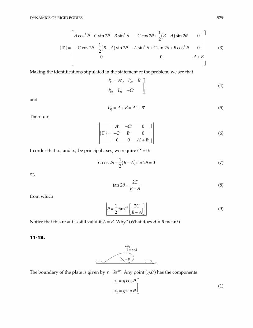
DYNAMICS OF RIGID BODIES 379
2 2
2 2
1cos sin 2 sin cos 2 sin 2 0
21
cos 2 sin 2 sin sin 2 cos 020 0
A C B C B A
C B A A C B
A B
I (3)
Making the identifications stipulated in the statement of the problem, we see that
11 22
12 21
,I A I B
I I C (4)
and
33I A B A B (5)
Therefore
00
0 0
A CC B
A BI (6)
In order that and be principal axes, we require C = 0: 1x 2x
1
cos 2 sin 2 02
C B A (7)
or,
2
tan 2C
B A (8)
from which
11 2tan
2C
B A (9)
Notice that this result is still valid if A = B. Why? (What does A = B mean?)
11-19.
" = 0
x2
x. "
" = '
" = '/2
1
The boundary of the plate is given by r ke . Any point ( , ) has the components
1
2
cos
sin
x
x (1)
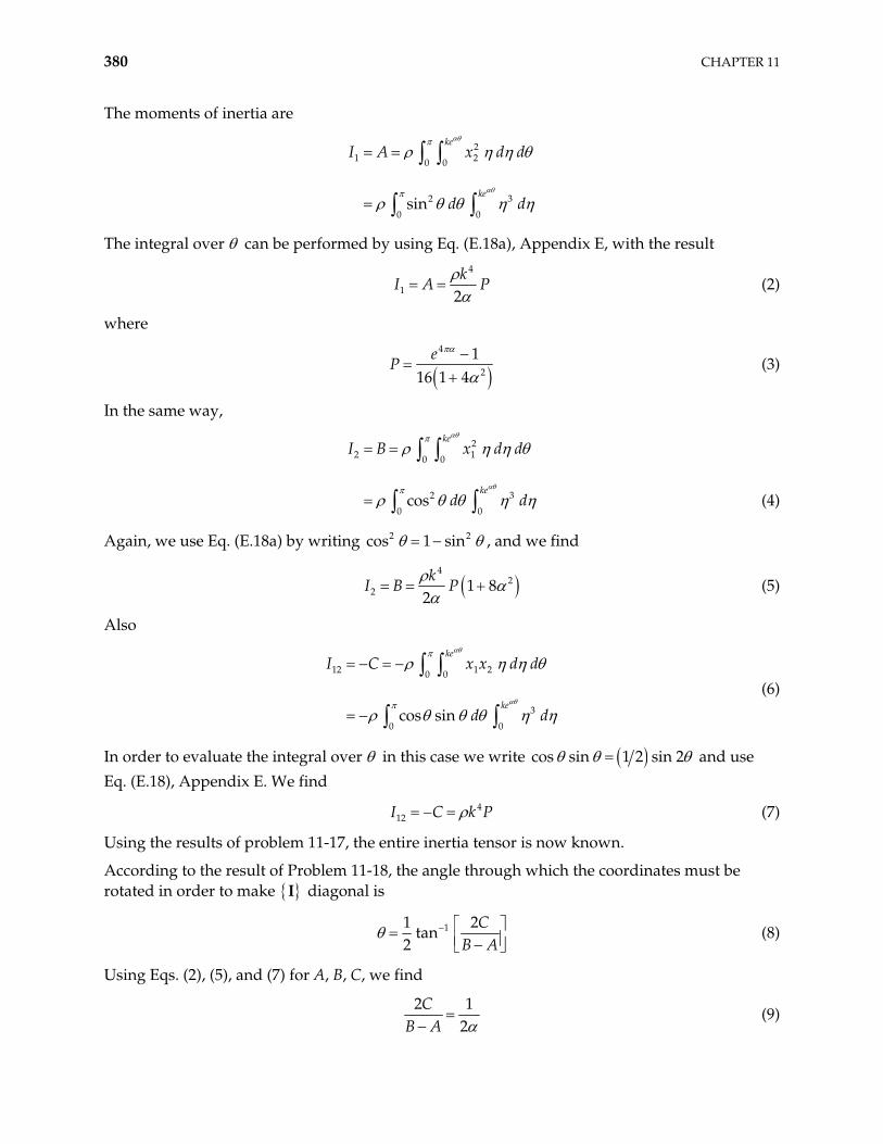
380 CHAPTER 11
The moments of inertia are
21 20 0
2 3
0 0sin
ke
ke
I A x d d
d d
The integral over can be performed by using Eq. (E.18a), Appendix E, with the result
4
1 2k
I A P (2)
where
4
2
116 1 4
eP (3)
In the same way,
22 10 0
2
0 0cos
ke
ke
I B x d d
d 3 d (4)
Again, we use Eq. (E.18a) by writing co 2s 1 sin2 , and we find
4
22 1 8
2k
I B P (5)
Also
12 1 20 0
3
0 0cos sin
ke
ke
I C x x d d
d d
(6)
In order to evaluate the integral over in this case we write cos sin 1 2 sin 2 and use Eq. (E.18), Appendix E. We find
(7) 412I C k P
Using the results of problem 11-17, the entire inertia tensor is now known.
According to the result of Problem 11-18, the angle through which the coordinates must be rotated in order to make I diagonal is
11 2tan
2C
B A (8)
Using Eqs. (2), (5), and (7) for A, B, C, we find
2 1
2C
B A (9)
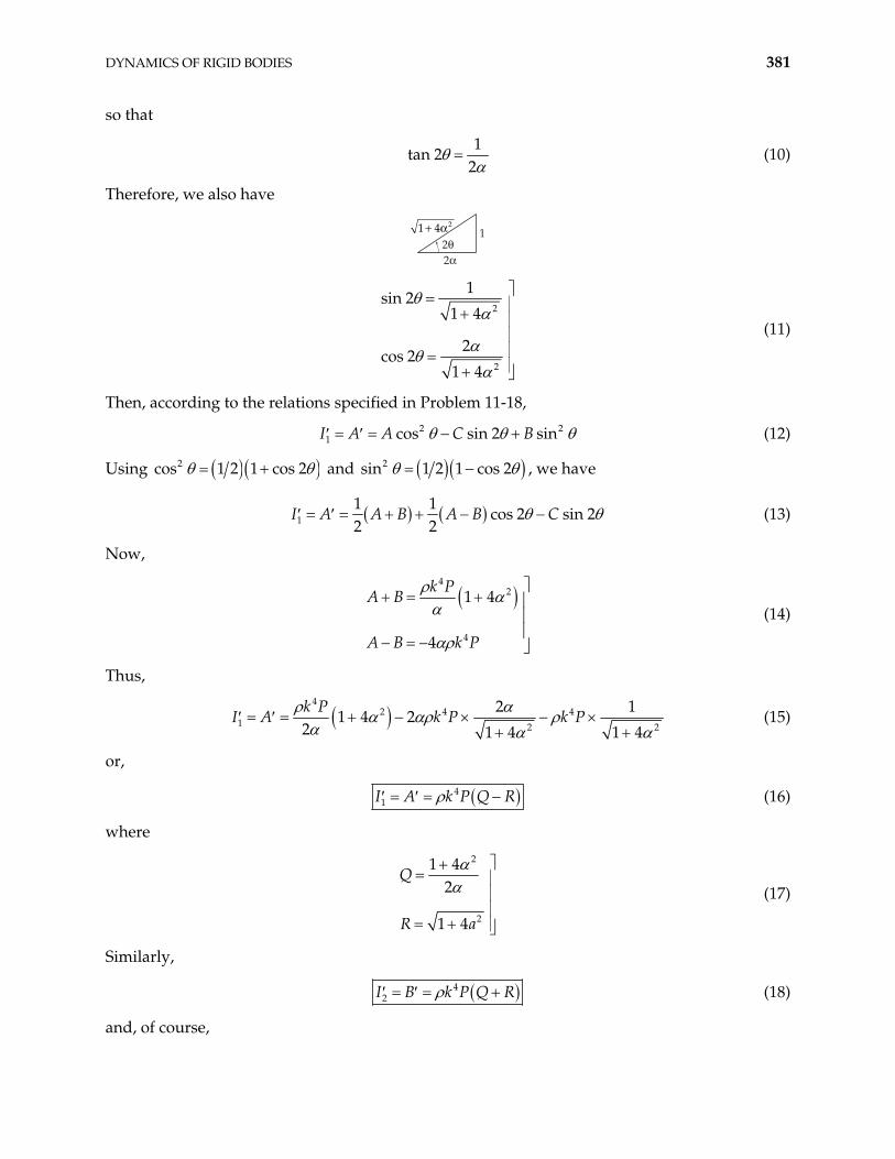
DYNAMICS OF RIGID BODIES 381
so that
1
tan 22
(10)
Therefore, we also have
2"2/
11 4 2+ /
2
2
1sin 2
1 4
2cos 2
1 4
(11)
Then, according to the relations specified in Problem 11-18,
21 cos sin 2 sinI A A C B 2 (12)
Using 2cos 1 2 1 cos 2 and 2sin 1 2 1 cos 2 , we have
11 1
cos 2 sin 22 2
A B A B CI A (13)
Now,
42
4
1 4
4
k PA B
A B k P
(14)
Thus,
4
2 4 41 2 2
2 11 4 2
2 1 4 1 4
k Pk P k PI A (15)
or,
41I A k P Q R (16)
where
2
2
1 42
1 4
Q
R a
(17)
Similarly,
42I B k P Q R (18)
and, of course,
382 CHAPTER 11
3I A B I I1 2 (19)
We can also easily verify, for example, that I12 0C .
11-20. We use conservation of energy. When standing upright, the kinetic energy is zero. Thus, the total energy is the potential energy
1 2b
E U mg
(2b
is the height of the center of mass above the floor.)
When the rod hits the floor, the potential energy is zero. Thus
22
12
E T I
where I is the rotational inertia of a uniform rod about an end. For a rod of length b, mass/length :
2 3end
0
1 13 3
b
I x dx b 2mb
Thus
2 22
16
T mb
By conservation of energy
1 2U T
2 212 6b
mg mb
3gb
11-21. Using I to denote the matrix whose elements are those of I , we can write
L I (11.54)
L I (11.54a)
We also have and and therefore we can express L and as x x xtx
tL L (11.55a)
t (11.55b)
substituting these expressions into Eq. (11.54), we have
DYNAMICS OF RIGID BODIES 383
t tL I
and multiplying on the left by ,
t tL I
or
tL I
by virture of Eq. (11.54a), we identify
tI I (11.61)
11-22. According to Eq. (11.61),
1
,ij ik k j
k l
I I (1)
Then,
1
,
1
,
,
ii ik k ii i k
k i ikk i
k k kkk k
tr I I
I
I I
I
(2)
so that
tr trI I (3)
This relation can be verified for the examples in the text by straightforward calculations.
Note: A translational transformation is not a similarity transformation and, in general, tr is not invariant under translation. (For example,
Itr I will be different for inertia tensors expressed in
coordinate system with different origins.)
11-23. We have
1I I (1)
Then,
384 CHAPTER 11
1
1
1
I I
I
I
so that,
I I (2)
This result is easy to verify for the various examples involving the cube.
11-24.
–a/2 a/2x2
x1
& 32
a
The area of the triangle is 23 4A a , so that the density is
2
43
M MA a
(1)
a) The rotational inertia with respect to an axis through the point of suspension (the origin) is
x2
x1
"
1
2 23 1 2 1 2
2 02 2
1 1 20 3
22
4 2
2
3 124 6
a
a x
I x x dx dx
dx x x dx
a Ma
2
(2)
When the triangle is suspended as shown and when = 0, the coordinates of the center of mass are 2(0, ,0)x , where
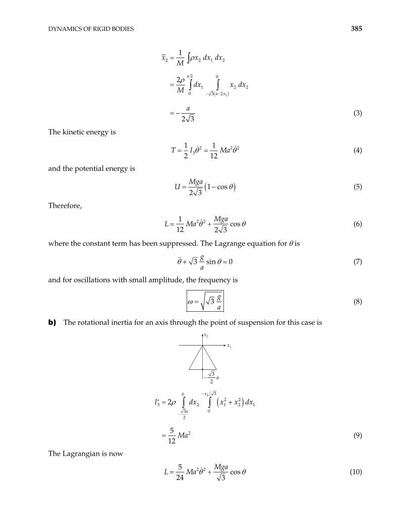
DYNAMICS OF RIGID BODIES 385
1
2 2 1 2
2 0
1 20 3 2
1
2
2 3
a
a x
x x dx dxM
dx x dxM
a
2
(3)
The kinetic energy is
23
1 12 12
T I Ma2 2 (4)
and the potential energy is
1 cos2 3Mga
U (5)
Therefore,
2 21cos
12 2 3Mga
L Ma (6)
where the constant term has been suppressed. The Lagrange equation for is
3 sin 0ga
(7)
and for oscillations with small amplitude, the frequency is
3ga
(8)
b) The rotational inertia for an axis through the point of suspension for this case is
x2
x1
& 32
a
2 302 2
3 2 1 203
2
2
2
512
x
a
I dx x x
Ma
1dx
(9)
The Lagrangian is now
2 25cos
24 3Mga
L Ma (10)
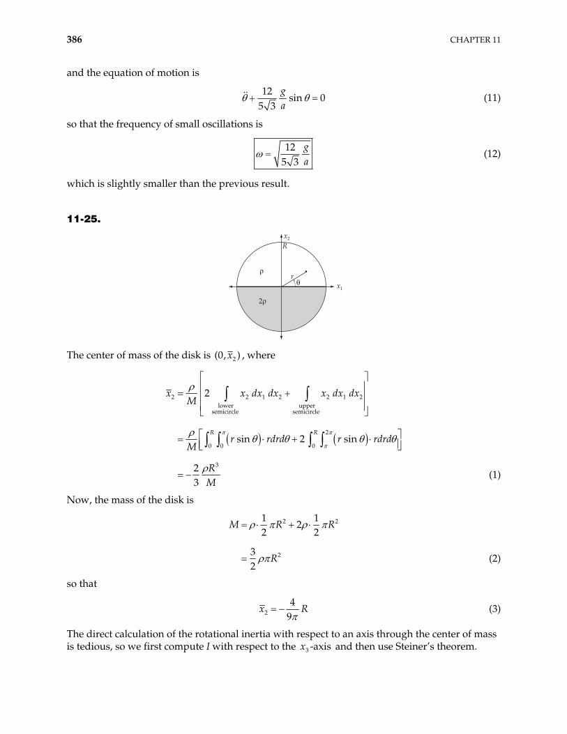
386 CHAPTER 11
and the equation of motion is
12
sin 05 3
ga
(11)
so that the frequency of small oscillations is
12
5 3ga
(12)
which is slightly smaller than the previous result.
11-25.
x2
x1
R
r
20
0"
The center of mass of the disk is 2(0, )x , where
2 2 1 2 2 1 2lower upper
semicircle semicircle
2
0 0 0
3
2
sin 2 sin
23
R R
x x dx dx x dx dxM
r rdrd r rdrdM
RM
(1)
Now, the mass of the disk is
2 2
2
1 12
2 2
32
M R
R
R
(2)
so that
24
9x R (3)
The direct calculation of the rotational inertia with respect to an axis through the center of mass is tedious, so we first compute I with respect to the and then use Steiner’s theorem. 3 -axisx
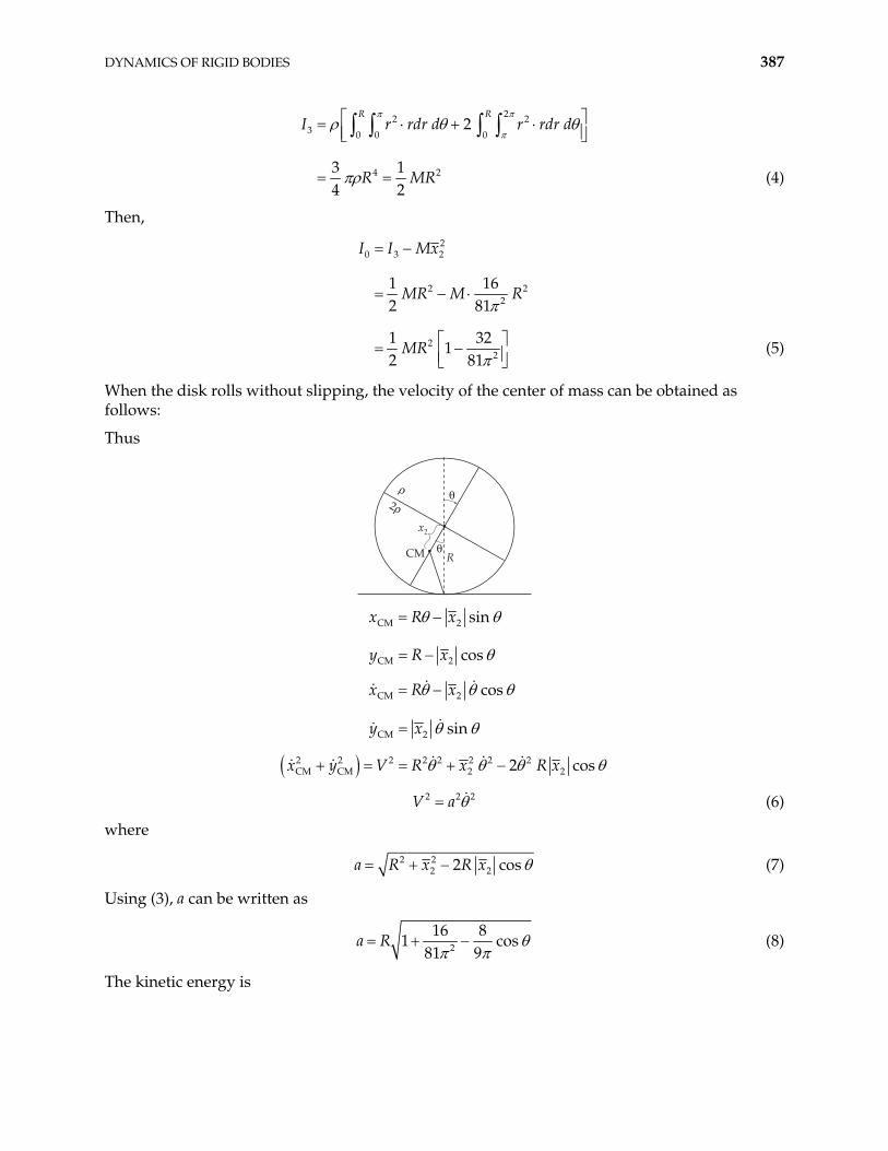
DYNAMICS OF RIGID BODIES 387
22 23 0 0 0
4 2
2
3 14 2
R RI r rdr d r rd
R MR
r d
(4)
Then,
20 3 2
2 22
22
1 12 81
1 321
2 81
I I Mx
6MR M R
MR (5)
When the disk rolls without slipping, the velocity of the center of mass can be obtained as follows:
Thus
RCM
"
"
CM 2
CM 2
sin
cos
x R x
y R x
200
x2
CM 2
CM 2
cos
sin
x R x
y x
2 2 2 2 2 2 2 2CM CM 2 22 cox y V R x R x s
2
2 2V a (6)
where
2 22 22 cosa R x R x (7)
Using (3), a can be written as
2
16 81
81 9a R cos (8)
The kinetic energy is
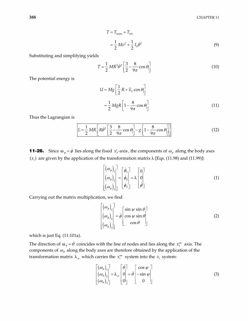
388 CHAPTER 11
trans rot
20
1 12 2
T T T
Mv I 2 (9)
Substituting and simplifying yields
2 21 3 8cos
2 2 9T MR (10)
The potential energy is
21
cos2
1 81 cos
2 9
U Mg R x
MgR (11)
Thus the Lagrangian is
21 3 8 8cos 1 cos
2 2 9 9R R gL M (12)
11-26. Since lies along the fixed 3 -axisx , the components of along the body axes
are given by the application of the transformation matrix [Eqs. (11.98) and (11.99)]: ( )ix
1 1
22
33
00 (1)
Carrying out the matrix multiplication, we find
1
2
3
sin sincos sin
cos (2)
which is just Eq. (11.101a).
The direction of coincides with the line of nodes and lies along the axis. The components of
1x along the body axes are therefore obtained by the application of the
transformation matrix which carries the xi system into the system: ix
1
2
3
cos0 sin0 0
(3)
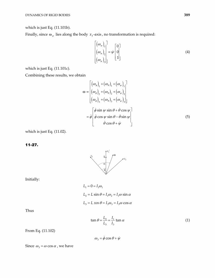
DYNAMICS OF RIGID BODIES 389
which is just Eq. (11.101b).
Finally, since lies along the body , no transformation is required: 3 -axisx
1
2
3
001
(4)
which is just Eq. (11.101c).
Combining these results, we obtain
11 1
22 2
33 3
sin sin cos
cos sin sin
cos
(5)
which is just Eq. (11.02).
11-27.
L
/
"
1x3x2
x3!
Initially:
1 1 1
2 1 2 1
3 3 3 3
0
sin sin
cos
L I
L L I I
L L xos I I
Thus
2 1
3 3
tan tanL IL I
(1)
From Eq. (11.102)
3 cos
Since 3 cos , we have

390 CHAPTER 11
cos cos (2)
From Eq. (11.131)
3 13
1
I II
(2) becomes
3
1
cos cosII
(3)
From (1), we may construct the following triangle
I3
I3 tan /
"
from which 31 22 2 2
3 1
stan
I
I Ico
Substituting into (3) gives
2 2 2 21 3
1
sin cosI II
11-28. From Fig. 11-7c we see that is along the 3 -axisx , is along the line of nodes, and is along the . Then, 3 -axx is
3e (1)
whee is the unit vector in the direction. 3e 3x
Projecting the lines of nodes into the 1 -x and 2 -axesx , we obtain
1 2cos sine e (2)
has components along all three of the xi axes. First, we write in terms of a component along the x and a component normal to this axis: 3 -axis
12 3sin cose e (3)
where
12 1 2sin cose e e (4)
Then,
1 2 3sin sin sin cos cose e e (5)
DYNAMICS OF RIGID BODIES 391
Collecting the various components, we have
1
2
3
cos sin sin
sin sin cos
cos
(6)
11-29. When the motion is vertical = 0. Then, according to Eqs. (11.153) and (11.154),
3P I P (1)
and using Eq. (11.159), we see that
3 3P P I (2)
Also, when = 0 (and ), the energy is [see Eq. (11.158)] 0
23 3
12
E I Mgh (3)
Furthermore, referring to Eq. (11.160),
23 3
12
E E I Mgh (3)
If we wish to examine the behavior of the system near = 0 in order to determine the conditions for stability, we can use the values of P , P , and E for = 0 in Eq. (11.161). Thus,
22 2
3 3212 2
12
1 cos1cos
2 2 sinI
I MghI
Mgh (5)
Changing the variable to z = cos and rearranging, Eq. (5) becomes
2
212 3 32
12
12 1
z 2 2z Mgh I z I wI
(6)
The questions concerning stability can be answered by examining this expression. First, we note that for physically real motion we must have 2 0z . Now, suppose that the top is spinning very rapidly, i.e., that 3 is large. Then, the term in the square brackets will be negative. In such a case, the only way to maintain the condition 2 0z is to have z = 1, i.e., = 0. Thus, the motion at = 0 will be stable as long as
2 212 3 34Mgh I I 0 (7)
or,
122 23 3
41
Mgh II
(8)
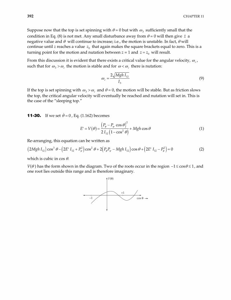
392 CHAPTER 11
Suppose now that the top is set spinning with = 0 but with 3 sufficiently small that the condition in Eq. (8) is not met. Any small disturbance away from = 0 will then give z a negative value and will continue to increase; i.e., the motion is unstable. In fact, will continue until z reaches a value 0z that again makes the square brackets equal to zero. This is a turning point for the motion and nutation between z = 1 and 0z z will result.
From this discussion it is evident that there exists a critical value for the angular velocity, c , such that for 3 c the motion is stable and for c there is nutation:
12
3
2c
Mgh II
(9)
If the top is set spinning with 3 c and = 0, the motion will be stable. But as friction slows the top, the critical angular velocity will eventually be reached and nutation will set in. This is the case of the “sleeping top.”
11-30. If we set , Eq. (1.162) becomes 0
2
212
coscos
2 1 cos
P PMgh
IE V (1)
Re-arranging, this equation can be written as 3 2 2
12 12 12 122 cos 2 cos 2 cos 2 0Mgh I E I P P P Mgh I E I P2 (2)
which is cubic in cos .
V( ) has the form shown in the diagram. Two of the roots occur in the region 1 cos 1, and one root lies outside this range and is therefore imaginary.
V(")
cos "–1
+1
DYNAMICS OF RIGID BODIES 393
11-31. The moments of inertia of the plate are
1 2
2
3 1 2
2
22
cos 2
1 cos 2
2 cos
I I
I
I I I
I
I
(1)
We also note that
1 2 2
22
1 cos 2
2 sin
I I I
I (2)
Since the plate moves in a force-free manner, the Euler equations are [see Eq. (11.114)]
1 2 1 2 3 3
2 3 2 3 1 1
3 1 3 1 2 2
0
0
0
I I I
I I I
I I I
(3)
Substituting (1) and (2) into (3), we find
2 22 1 2 2 3
2 2 3 2 1
2 3 1 2 2
2 sin 2 cos 0
cos 2 cos 2 0
0
I I
I I
I I
(4)
These equations simplify to
23 1 2
1 2 3
2 3 1
tan
(5)
From which we can write
21 2 3 2 2 1 1 3 3 cot (6)
Integrating, we find
2 2 2 2 2 2 2 22 2 1 1 3 30 0 cot 0 cot (7)
Now, the initial conditions are
394 CHAPTER 11
1
2
3
0 cos
0 0
0 sin
(8)
Therefore, the equations in (7) become
22 2 2 2 2 2 22 1 3cos cot cos (9)
From (5), we can write
2 22 3
21 (10)
and from (9), we have 2 2 21 3 cot . Therefore, (10) becomes
22 3 cot (11)
and using 2 2 2 2 23 2sin tan from (9), we can write (11) as
22 2 2 22
cottan sin
(12)
Since 2 2d dt , we can express this equation in terms of integrals as
22 2 2 22
cottan sin
ddt (13)
Using Eq. (E.4c), Appendix E, we find
1 2 tan1tanh cot
tan sin sint (14)
Solving for 2 ,
2 cos tanh sint t (15)
11-32.
a) The exact equation of motion of the physical pendulum is
sin 0I MgL
where , so we have 2I Mk
2 singLk
or
2
d cosdd d
gLt k
or
DYNAMICS OF RIGID BODIES 395
2d d cogLk
s
so
22
2cos
gLa
k
where a is a constant determined by the initial conditions. Suppose that at t , 0 0 and at
that initial position the angular velocity of the pendulum is zero, we find 02
2a
kcos
gl. So
finally
02
2cos cos
glk
b) One could use the conservation of energy to find the angular velocity of the pendulum at any angle , but it is exactly the result we obtained in a), so at 01 , we have
102
2cos cos 53.7 s
gLk
11-33. Cats are known to have a very flexible body that they can manage to twist around to a feet-first descent while falling with conserved zero angular momentum. First they thrust their back legs straight out behind their body and at the same time they tuck their front legs in. Extending their back legs helps to resist spinning, since rotation velocity evidently is inversely proportional to inertia momentum. This allows the cat to twist their body differently to preserve zero angular momentum: the front part of the body twisting more than the back. Tucking the front legs encourages spinning to a downward direction preparing for touchdown and as this happens, cats can easily twist the rear half of their body around to catch up with the front.
However, whether or not cats land on their feet depends on several factors, notably the distance they fall, because the twist maneuver takes a certain time, apparently around 0.3 sec. Thus the minimum height required for cats falling is about 0.5m.
11-34. The Euler equation, which describes the rotation of an object about its symmetry axis, say 0x, is
x x y z y z xI I I N
x
where xN b is the component of torque along Ox. Because the object is symmetric about Ox, we have y zII , and the above equation becomes
0dd
xxx x x
b tII b e
t x

396 CHAPTER 11
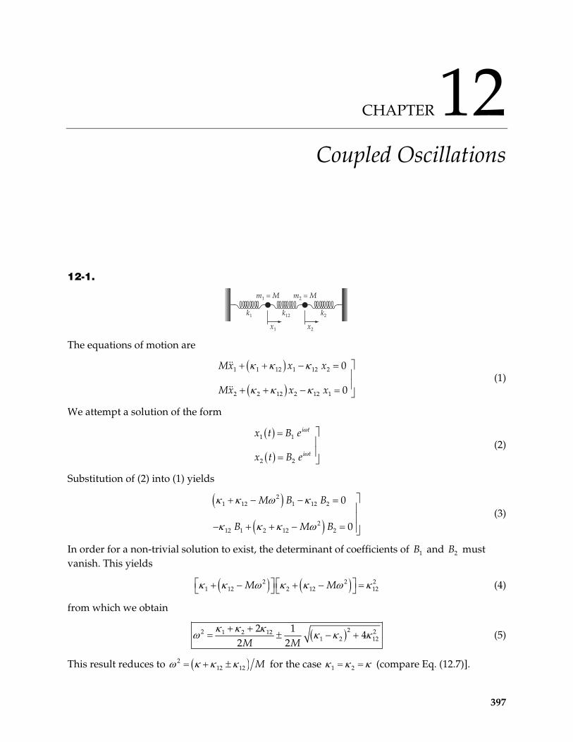
CHAPTER 12 Coupled Oscillations
12-1.
m1 = M
k1
x1
k12 k2
m2 = M
x2 The equations of motion are
1 1 12 1 12 2
2 2 12 2 12 1
0
0
Mx x x
Mx x x (1)
We attempt a solution of the form
1 1
2 2
i t
i t
x t B e
x t B e (2)
Substitution of (2) into (1) yields
21 12 1 12 2
212 1 2 12 2
0
0
M B B
B M B (3)
In order for a non-trivial solution to exist, the determinant of coefficients of and must vanish. This yields
1B 2B
2 21 12 2 12 12M M 2 (4)
from which we obtain
21 2 121 2 12
2 14
2 2M M2 2 (5)
This result reduces to 212 12 M for the case 1 2 (compare Eq. (12.7)].
397
398 CHAPTER 12
If were held fixed, the frequency of oscillation of m would be 2m 1
201 1 12
1M
(6)
while in the reverse case, would oscillate with the frequency 2m
202 2 12
1M
(7)
Comparing (6) and (7) with the two frequencies, and , given by (5), we find
22 21 2 12 1 2 12
12 4
2M
21 2 12 1 2 1 12 0
1 12
2M M 1 (8)
so that
01 (9)
Similarly,
22 21 2 12 1 2 12
12 4
2M
21 2 12 1 2 2 12 0
1 12
2M M 2 (10)
so that
02 (11)
If , then the ordering of the frequencies is 1 2
01 02 (12)
12-2. From the preceding problem we find that for 12 1 2,
1 12 2 121 2;
M M (1)
If we use
101 02;
M M2 (2)
then the frequencies in (1) can be expressed as
COUPLED OSCILLATIONS 399
121 01 01 1
1
122 02 02 2
2
1 1
1 1
(3)
where
12 121 2
1 2
;2 2
(4)
For the initial conditions [Eq. 12.22)],
1 2 1 20 , 0 0, 0 0, 0 0x x x ,x D (5)
the solution for 1x t is just Eq. (12.24):
1 2 1 21 cos cos
2 2D t tx t (6)
Using (3), we can write
1 2 01 02 1 01 2 02
2 2 (7)
1 2 01 02 1 01 2 02
2 2 (8)
Then,
1 cos cosx t D t t t t (9)
Similarly,
1 2 1 22 sin sin
2 2
sin sin
x t D t t
D t t t t (10)
Expanding the cosine and sine functions in (9) and (10) and taking account of the fact that and are small quantities, we find, to first order in the ’s,
1 cos cos sin cos cos sinD t t t t t t t tx t (11)
2 sin sin cos sin sin cosD t t t t t t t tx t (12)
When either 1x t or 2x t reaches a maximum, the other is at a minimum which is greater than zero. Thus, the energy is never transferred completely to one of the oscillators.
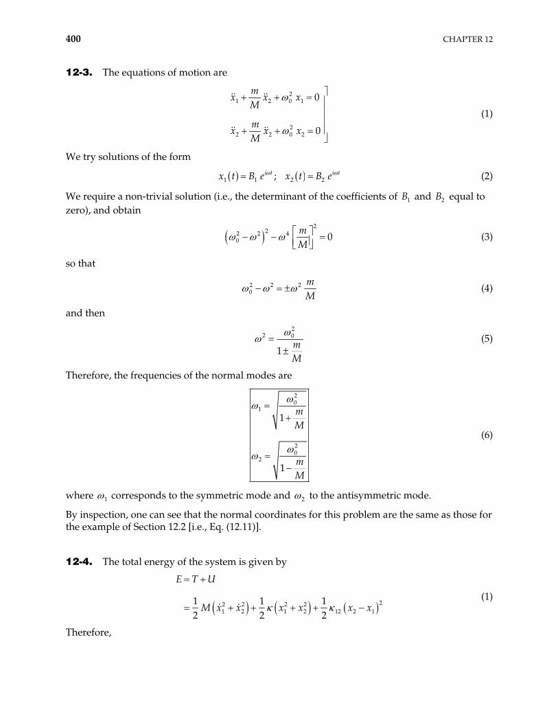
400 CHAPTER 12
12-3. The equations of motion are
21 2 0 1
22 2 0 2
0
0
mx x x
M
mx x x
M
(1)
We try solutions of the form
1 1 2 2;i t i tx t B e x t B e (2)
We require a non-trivial solution (i.e., the determinant of the coefficients of B and equal to zero), and obtain
1 2B
2
22 2 40 0
mM
(3)
so that
2 2 20
mM
(4)
and then
2
2 0
1 mM
(5)
Therefore, the frequencies of the normal modes are
20
1
20
2
1
1
mM
mM
(6)
where 1 corresponds to the symmetric mode and 2 to the antisymmetric mode.
By inspection, one can see that the normal coordinates for this problem are the same as those for the example of Section 12.2 [i.e., Eq. (12.11)].
12-4. The total energy of the system is given by
22 2 2 2
1 2 1 2 12 2 11 1 12 2 2
E T U
M x x x x x x (1)
Therefore,
COUPLED OSCILLATIONS 401
1 1 2 2 1 1 2 2 12 2 1 2 1
1 1 12 2 1 1 2 2 12 2 1
1 12 1 12 2 1 2 12 1 12 2 2
dEM x x x x x x x x x x x x
dt
Mx x x x x Mx x x x x
Mx x x x Mx x x x
2
(2)
which exactly vanishes because the coefficients of and are the left-hand sides of Eqs. (12.1a) and (12.1b).
1x 2x
An analogous result is obtained when T and U are expressed in terms of the generalized coordinates 1 and 2 defined by Eq. (12.11):
2 21 2
14
T M (3)
2 21 2 12
1 14 2
U 21 (4)
Therefore,
1 12 1 1 2 2 2dE
M Mdt
2 2 (5)
which exactly vanishes by virtue of Eqs. (12.14).
When expressed explicitly in terms of the generalized coordinates, it is evident that there is only one term in the energy that has as a coefficient (namely, 12
212 1
1
), and through Eq. (12.15) we see that this implies that such a term depends on the ’s and 1C , but not on the ’s and 2C 2 .
To understand why this is so, it is sufficient to recall that 1 is associated with the anitsymmetrical mode of oscillation, which obviously must have 12 as a parameter. On the other hand, 2 is associated to the symmetric mode, 1 2x t x t , 1 2x t x t , in which both masses move as if linked together with a rigid, massless rod. For this mode, therefore, if the spring connecting the masses is changed, the motion is not affected.
12-5. We set . Then, the equations of motion are 1 2 12
1 1 1 2
2 2 2 1
2 0
2 0
m x x x
m x x x (1)
Assuming solutions of the form
1 1
2 2
i t
i t
x t B e
x t B e (2)
we find that the equations in (1) become
402 CHAPTER 12
21 1 2
21 2 2
2 0
2 0
m B B
B m B (3)
which lead to the secular equation for 2 :
2 21 22 2m m 2 (4)
Therefore,
2
1 2
31 1
m m (5)
where 1 2 1 2m m m m
1 2
is the reduced mass of the system. Notice that (5) agrees with Eq.
(12.8) for the case m m and M 12 . Notice also that 2 is always real and positive since the maximum value of 1 m23 m is 3 4 . (Show this.)
Inserting the values for 1 and 2 into either of the equations in (3), we find1
111 21
1 2
32 1 1
ma a
m m (6)
and
112 22
1 2
32 1 1
ma
m ma (7)
Using the orthonormality condition produces
111
1a
D (8)
1 2 1 22
2 1 221
1
32 1 1m m m mm m m
Da (9)
where
2
2 211 2 1 1 2 2
2 2 1 2
322 2 1
m mm m m
m m m m1 2m
D m (10)
The second eigenvector has the components
1 2 1 22
2 1 212
2
32 1 1m m m mm m m
Da (11)
1 Recall that when we use 1 , we call the coefficients 1 1 a11 and 2 1 a21 , etc.
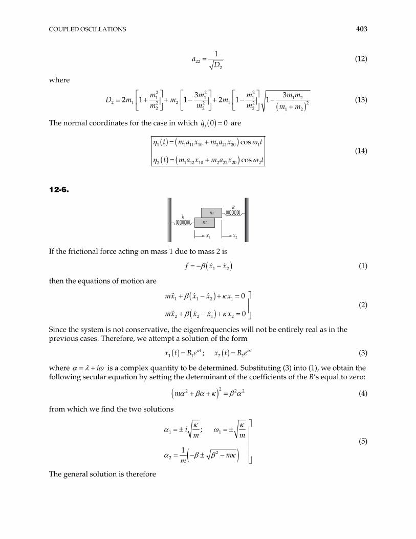
COUPLED OSCILLATIONS 403
222
1a
D (12)
where
2 2 21 1 1
2 1 2 1 22 2 22 2 2 1 2
3 32 1 1 2 1 1
m m m mm m
m m m m m1 2m
D m (13)
The normal coordinates for the case in which 0jq 0 are
1 1 11 10 2 21 20
2 1 12 10 2 22 20
cos
cos
t m a x m a x t
t m a x m a x
1
2t (14)
12-6.
mm
mmk
k
x1 x2 If the frictional force acting on mass 1 due to mass 2 is
1 2f x x (1)
then the equations of motion are
1 1 2 1
2 2 1 2
0
0
mx x x x
mx x x x (2)
Since the system is not conservative, the eigenfrequencies will not be entirely real as in the previous cases. Therefore, we attempt a solution of the form
1 1 2 2;tx t B e x t B e t (3)
where i is a complex quantity to be determined. Substituting (3) into (1), we obtain the following secular equation by setting the determinant of the coefficients of the B’s equal to zero:
22m 2 2 (4)
from which we find the two solutions
1 1
22
;
1
im m
mm
(5)
The general solution is therefore
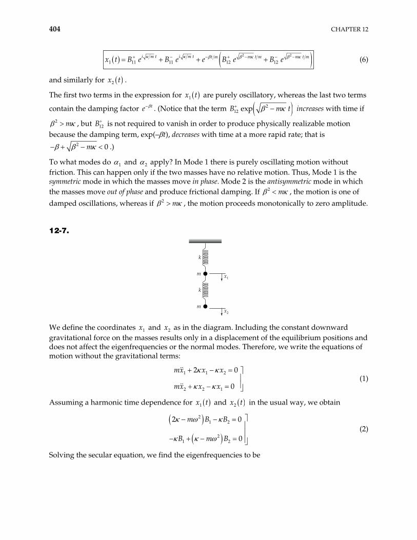
404 CHAPTER 12
2 2
1 11 11 12 12i m t i m t m t m m t mt mB e B e e B e B ex t (6)
and similarly for 2x t .
The first two terms in the expression for 1x t are purely oscillatory, whereas the last two terms
contain the damping factor te . (Notice that the term 212 expB m t increases with time if
2 m , but is not required to vanish in order to produce physically realizable motion because the damping term, exp(– t), decreases with time at a more rapid rate; that is
12B
2 0m .)
To what modes do 1 and 2 apply? In Mode 1 there is purely oscillating motion without friction. This can happen only if the two masses have no relative motion. Thus, Mode 1 is the symmetric mode in which the masses move in phase. Mode 2 is the antisymmetric mode in which the masses move out of phase and produce frictional damping. If 2 m , the motion is one of damped oscillations, whereas if 2 m , the motion proceeds monotonically to zero amplitude.
12-7.
m
k
m
k
x1
x2
We define the coordinates and as in the diagram. Including the constant downward gravitational force on the masses results only in a displacement of the equilibrium positions and does not affect the eigenfrequencies or the normal modes. Therefore, we write the equations of motion without the gravitational terms:
1x 2x
1 1 2
2 2 1
2 0
0
mx x x
mx x x (1)
Assuming a harmonic time dependence for 1 tx and 2x t in the usual way, we obtain
21 2
21 2
2 0
0
m B B
B m B (2)
Solving the secular equation, we find the eigenfrequencies to be
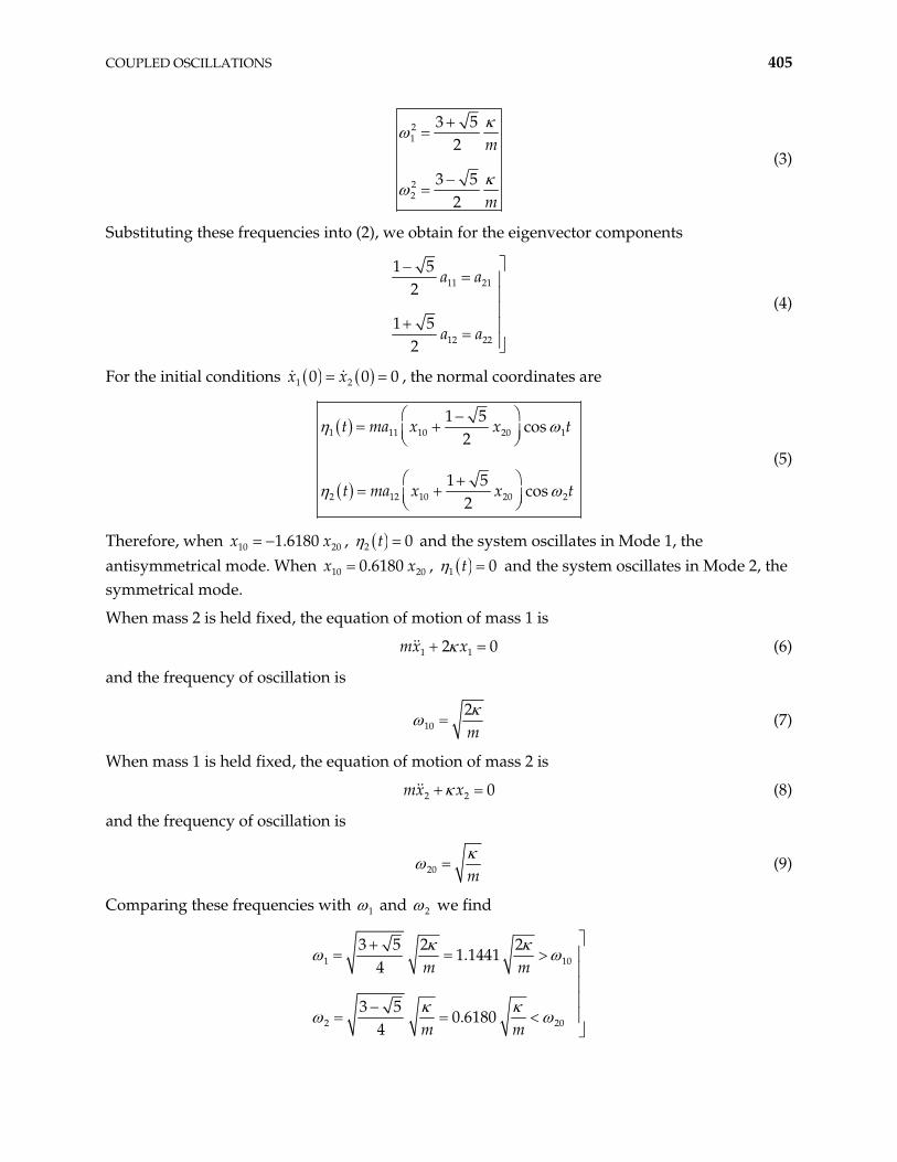
COUPLED OSCILLATIONS 405
21
22
3 52
3 52
m
m
(3)
Substituting these frequencies into (2), we obtain for the eigenvector components
11 21
12 22
1 52
1 52
a a
a a
(4)
For the initial conditions 1 20 0x x 0 , the normal coordinates are
1 11 10 20
2 12 10 20
1 5cos
2
1 5cos
2
t ma x x t
t ma x x t
1
2
(5)
Therefore, when , 10 201.6180x x 2 0t and the system oscillates in Mode 1, the antisymmetrical mode. When , 10 20.6180x x 0 1 0t and the system oscillates in Mode 2, the symmetrical mode.
When mass 2 is held fixed, the equation of motion of mass 1 is
1 12mx x 0 (6)
and the frequency of oscillation is
102m
(7)
When mass 1 is held fixed, the equation of motion of mass 2 is
2 2 0mx x (8)
and the frequency of oscillation is
20 m (9)
Comparing these frequencies with 1 and 2 we find
1 1
2 2
3 5 2 21.1441
4
3 50.6180
4
m m
m m
0
0
406 CHAPTER 12
Thus, the coupling of the oscillators produces a shift of the frequencies away from the uncoupled frequencies, in agreement with the discussion at the end of Section 12.2.
12-8. The kinetic and potential energies for the double pendulum are given in Problem 7-7. If we specialize these results to the case of small oscillations, we have
2 2 21 2 1 2
12 2
2T m (1)
2 21 2
12
2U mg (2)
where 1 refers to the angular displacement of the upper pendulum and 2 to the lower pendulum, as in Problem 7-7. (We have also discarded the constant term in the expression for the potential energy.)
Now, according to Eqs. (12.34),
,
12 jk j k
j k
T m q q (3)
,
12 jk j k
j k
U A q q (4)
Therefore, identifying the elements of m and A , we find
2 2 11 1
mm (5)
2 00 1
mgA (6)
and the secular determinant is
2 2
2 2
2 20
g
g (7)
or,
2 2 42 2g g
0 (8)
Expanding, we find
2
4 24 2g g
0 (9)
which yields
COUPLED OSCILLATIONS 407
2 2 2g
(10)
and the eigenfrequencies are
1
2
2 2 1.848
2 2 0.765
g g
g g (11)
To get the normal modes, we must solve
2 0jk r jk jrj
A m a
For k = 1, this becomes:
2 211 11 1 21 21 2 0r r r rA m a A m a
For r = 1:
2 211 212 2 2 2 2 2
g gmg m a m a 0
Upon simplifying, the result is
21 112a a
Similarly, for r = 2, the result is
22 122a a
The equations
1 11 1 12
2 21 1 22
x a a
x a a
2
2
can thus be written as
1 11 1 2212
x a a 2
1 11 1 22 22x a a
Solving for 1 and 2 :
1 2 11 2
2211
2 2;
22 2x x x x
aa2
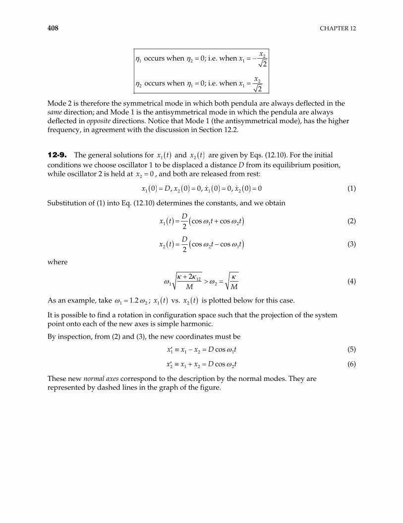
408 CHAPTER 12
21 2 1
22 1 1
occurs when 0; i.e. when 2
occurs when 0; i.e. when 2
xx
xx
Mode 2 is therefore the symmetrical mode in which both pendula are always deflected in the same direction; and Mode 1 is the antisymmetrical mode in which the pendula are always deflected in opposite directions. Notice that Mode 1 (the antisymmetrical mode), has the higher frequency, in agreement with the discussion in Section 12.2.
12-9. The general solutions for 1x t and 2x t are given by Eqs. (12.10). For the initial conditions we choose oscillator 1 to be displaced a distance D from its equilibrium position, while oscillator 2 is held at , and both are released from rest: 2 0x
1 2 1 20 , 0 0, 0 0, 0x x x 0x D (1)
Substitution of (1) into Eq. (12.10) determines the constants, and we obtain
1 1cos cos2D
x t t t2 (2)
2 2cos cos2D
x t t t1 (3)
where
121 2
2M M
(4)
As an example, take 1 21.2 ; 1x t vs. 2x t is plotted below for this case.
It is possible to find a rotation in configuration space such that the projection of the system point onto each of the new axes is simple harmonic.
By inspection, from (2) and (3), the new coordinates must be
1 1 2 1cosx x x D t (5)
2 1 2 2cosx x x D t (6)
These new normal axes correspond to the description by the normal modes. They are represented by dashed lines in the graph of the figure.
COUPLED OSCILLATIONS 409
0.2
0.2
–0.5
0.4
0.6
0.8
1.0 0.4 0.6 0.8 1.0
! "2
52
t =
! "2
32
t =
! "2 3t =
! "2 2t =
7"2
x2(t)/D x2#
x1#
x1(t)/D
!2t = "
3"
4"
!2t = 2"
!1 = 1.2 !2
!2t = 0
12-10. The equations of motion are
1 1 12 1 12 2 0
2 2 12 2 12 1
cos
0
mx bx x x F t
mx bx x x (1)
The normal coordinates are the same as those for the undamped case [see Eqs. (12.11)]:
1 1 2 2 1;x x x x2 (2)
Expressed in terms of these coordinates, the equations of motion become
2 1 2 1 12 2 1 12 2 1 0
2 1 2 1 12 2 1 12 2 1
2 cos
0
m b F
m b
t (3)
By adding and subtracting these equations, we obtain the uncoupled equations:
0121 1 1
02 2 2
2cos
cos
Fbt
m m m
Fbt
m m m
(4)
With the following definitions,
410 CHAPTER 12
2 121
22
0
2
2
bm
m
m
FA
m
(5)
the equations become
2
1 1 1 1
22 2 2 2
2 c
2 c
os
os
A t
A t (6)
Referring to Section 3.6, we see that the solutions for 1 t and 2 t are exactly the same as that given for x(t) in Eq. (3.62). As a result 1 t exhibits a resonance at 1 and 2 t exhibits a resonance at 2 .
12-11. Taking a time derivative of the equations gives q I
11 2 0
ILI MI
C
22 1 0
ILI MI
C
Assume 1 1i tI B e , 2 2
i tI B e ; and substitute into the previous equations. The result is
2 21 1 2
10i t i t i tLB e B e M B e
C
2 22 2 1
10i t i t i tLB e B e M B e
C
These reduce to
2 21 2
10B L B M
C
2 21 2
10B M B L
C
This implies that the determinant of coefficients of B and must vanish (for a non-trivial solution). Thus
1 2B
COUPLED OSCILLATIONS 411
2 2
2 2
1
01
L MC
M LC
2
22 210L M
C
2 21L M
C
or
2 1C L M
Thus
1
2
1
1
C L M
C L M
12-12. From problem 12-11:
1 1 21
0LI I MIC
(1)
2 2 11
0LI I MIC
(2)
Solving for in (1) and substituting into (2) and similarly for I , we have 1I 2
2
1 1 2
2
2 2 1
10
10
M ML I I I
L C CL
M ML I I I
L C CL
(3)
If we identify
2
12
11
Mm L
L
MLC
MC L
(4)
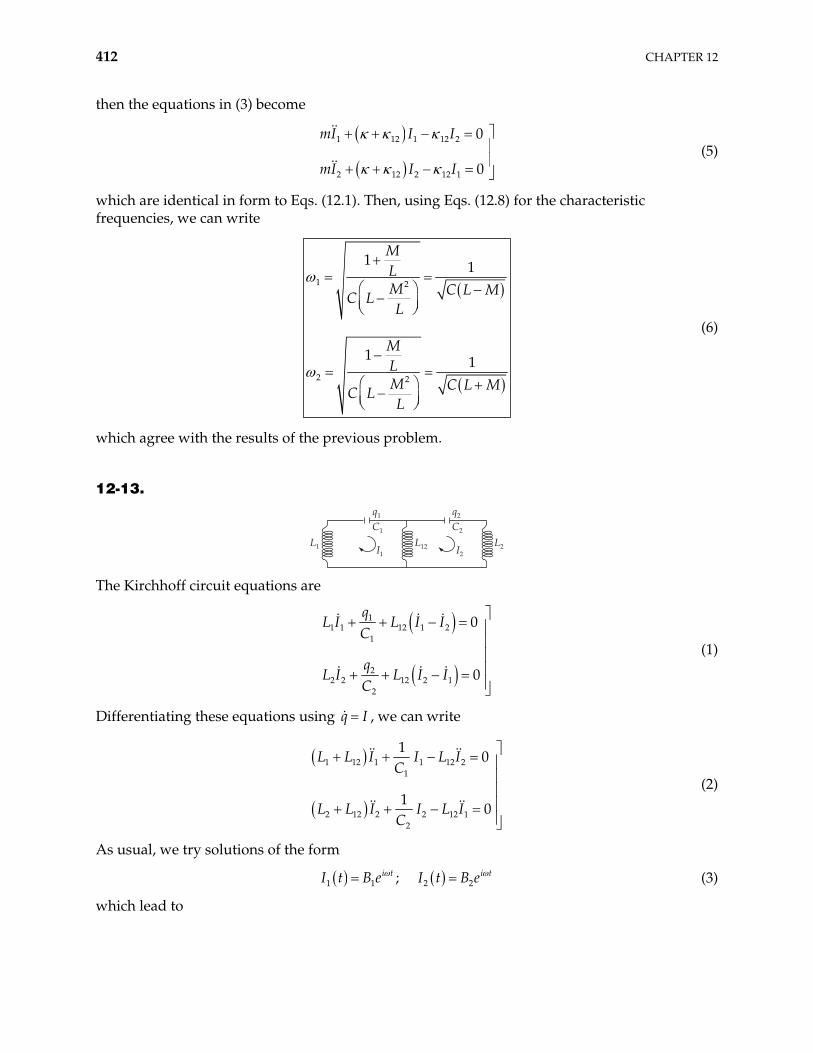
412 CHAPTER 12
then the equations in (3) become
1 12 1 12 2
2 12 2 12 1
0
0
mI I I
mI I I (5)
which are identical in form to Eqs. (12.1). Then, using Eqs. (12.8) for the characteristic frequencies, we can write
1 2
2 2
1 1
1 1
MLM C L MC LL
MLM C L MC LL
(6)
which agree with the results of the previous problem.
12-13.
I1
C1
q1
I2
C2
q2
L1 L12 L2
The Kirchhoff circuit equations are
11 1 12 1 2
1
22 2 12 2 1
2
0
0
qL I L I I
C
qL I L I I
C
(1)
Differentiating these equations using q I , we can write
1 12 1 1 12 21
2 12 2 2 12 12
10
10
L L I I L IC
L L I I L IC
(2)
As usual, we try solutions of the form
1 1 2 2;i t i tI t B e I t B e (3)
which lead to
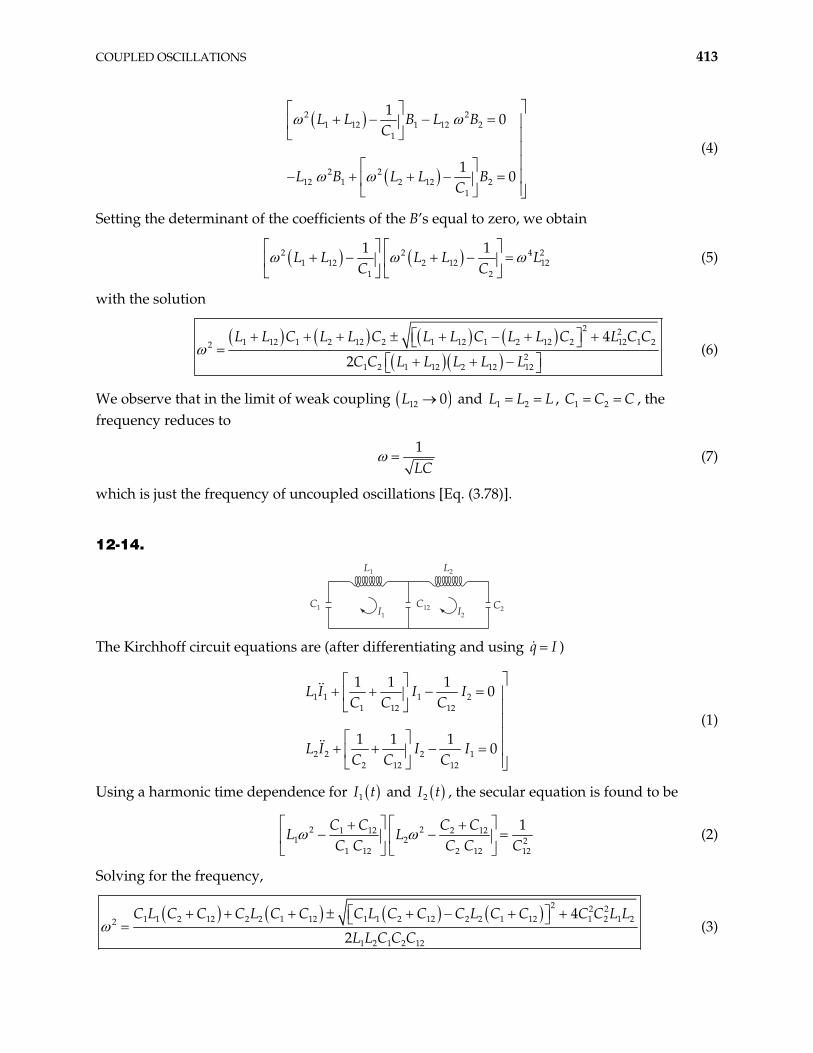
COUPLED OSCILLATIONS 413
2 21 12 1 12 2
1
2 212 1 2 12 2
1
10
10
L L B L BC
L B L L BC
(4)
Setting the determinant of the coefficients of the B’s equal to zero, we obtain
2 21 12 2 12 1
1 2
1 1L L L L L
C C4 2
2 (5)
with the solution
2 2
1 12 1 2 12 2 1 12 1 2 12 2 12 1 222
1 2 1 12 2 12 12
4
2
L L C L L C L L C L L C L C C
C C L L L L L (6)
We observe that in the limit of weak coupling 12 0L and 1 2L L L , C C , the frequency reduces to
1 2 C
1LC
(7)
which is just the frequency of uncoupled oscillations [Eq. (3.78)].
12-14.
I1
C1 C12 I2C2
L1 L2
The Kirchhoff circuit equations are (after differentiating and using q I )
1 1 1 21 12 12
2 2 2 12 12 12
1 1 10
1 1 10
L I I IC C C
L I I IC C C
(1)
Using a harmonic time dependence for 1I t and 2 tI , the secular equation is found to be
2 21 12 2 121 2 2
1 12 2 12 12
1C C C CL L
C C C C C (2)
Solving for the frequency,
2 2 21 1 2 12 2 2 1 12 1 1 2 12 2 2 1 12 1 2 1 22
1 2 1 2 12
4
2
C L C C C L C C C L C C C L C C C C L L
L L C C C (3)
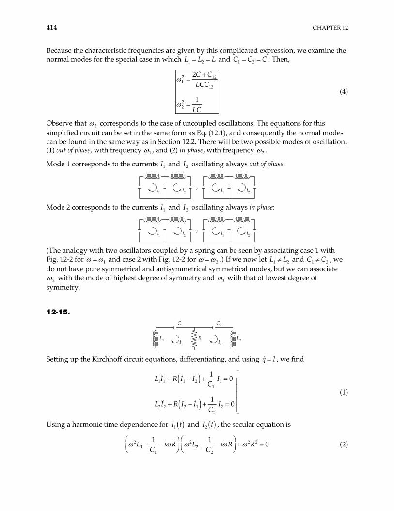
414 CHAPTER 12
Because the characteristic frequencies are given by this complicated expression, we examine the normal modes for the special case in which 1 2L L L and C C1 2 C . Then,
2 121
12
22
2
1
C CLCC
LC
(4)
Observe that 2 corresponds to the case of uncoupled oscillations. The equations for this simplified circuit can be set in the same form as Eq. (12.1), and consequently the normal modes can be found in the same way as in Section 12.2. There will be two possible modes of oscillation: (1) out of phase, with frequency 1 , and (2) in phase, with frequency 2 .
Mode 1 corresponds to the currents and oscillating always out of phase: 1I 2I
;I1 I2 I1 I2
Mode 2 corresponds to the currents and oscillating always in phase: 1I 2I
;I1 I2 I1 I2
(The analogy with two oscillators coupled by a spring can be seen by associating case 1 with Fig. 12-2 for 1 and case 2 with Fig. 12-2 for 2 .) If we now let and , we do not have pure symmetrical and antisymmetrical symmetrical modes, but we can associate
1L L2 21C C
2 with the mode of highest degree of symmetry and 1 with that of lowest degree of symmetry.
12-15.
I1
C1
I2
C2
L1 R L2
Setting up the Kirchhoff circuit equations, differentiating, and using q I , we find
1 1 1 2 11
2 2 2 1 22
10
10
L I R I I IC
L I R I I IC
(1)
Using a harmonic time dependence for 1I t and 2 tI , the secular equation is
2 21 2
1 2
1 10L i R L i R R
C C2 2 (2)
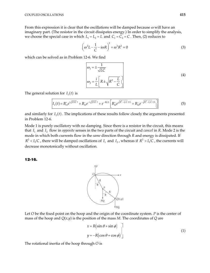
COUPLED OSCILLATIONS 415
From this expression it is clear that the oscillations will be damped because will have an imaginary part. (The resistor in the circuit dissipates energy.) In order to simplify the analysis, we choose the special case in which 1 2L L L and 1 2C C C . Then, (2) reduces to
2
2 10L i R R
C2 2 (3)
which can be solved as in Problem 12-6. We find
1
22
1LC
i LR R
L C
(4)
The general solution for is 1I t
2 21 1
1 11 11 12 12i LC t i LC t R L C t L R L C t LRt LB e B e e B e B eI t (5)
and similarly for . The implications of these results follow closely the arguments presented in Problem 12-6.
2I t
Mode 1 is purely oscillatory with no damping. Since there is a resistor in the circuit, this means that and flow in opposite senses in the two parts of the circuit and cancel in R. Mode 2 is the mode in which both currents flow in the same direction through R and energy is dissipated. If
1I 2I
2 CR L , there will be damped oscillations of and , whereas if 1I 2I 2R L C , the currents will decrease monotonically without oscillation.
12-16.
O
y
x
R
PR
Mg Q(x,y)
Mg
$
%
Let O be the fixed point on the hoop and the origin of the coordinate system. P is the center of mass of the hoop and Q(x,y) is the position of the mass M. The coordinates of Q are
sin sin
cos cos
x R
y R (1)
The rotational inertia of the hoop through O is
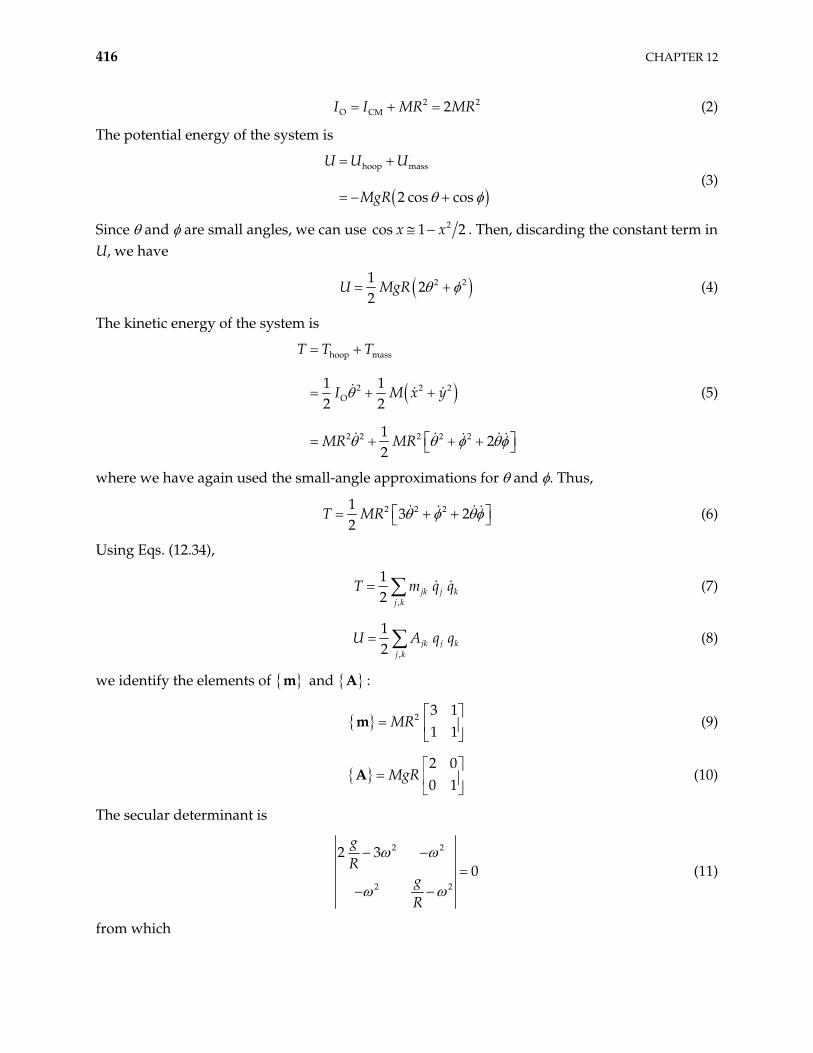
416 CHAPTER 12
(2) 2O CM 2I I MR MR2
The potential energy of the system is
hoop mass
2 cos cos
U U U
MgR (3)
Since and are small angles, we can use 2s 1 2x xco . Then, discarding the constant term in U, we have
2 212
2U MgR (4)
The kinetic energy of the system is
hoop mass
2 2 2O
2 2 2 2 2
1 12 2
12
2
T T T
I M x y
MR MR
(5)
where we have again used the small-angle approximations for and . Thus,
2 2 213 2
2T MR (6)
Using Eqs. (12.34),
,
12 jk j k
j k
T m q q (7)
,
12 jk j k
j k
U A q q (8)
we identify the elements of m and A :
2 3 11 1
MRm (9)
2 00 1
MgRA (10)
The secular determinant is
2 2
2 2
2 30
gR
gR
(11)
from which
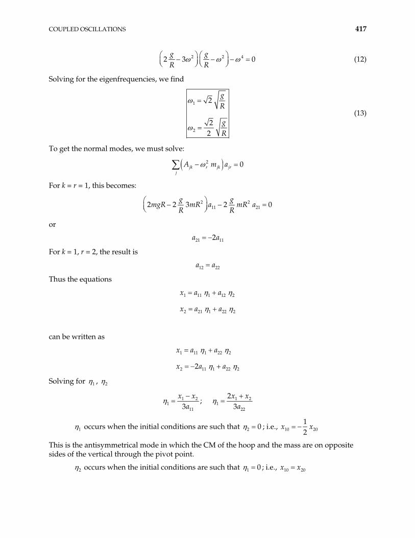
COUPLED OSCILLATIONS 417
2 2 42 3g gR R
0 (12)
Solving for the eigenfrequencies, we find
1
2
2
22
gR
gR
(13)
To get the normal modes, we must solve:
2 0jk r jk jrj
A m a
For k = r = 1, this becomes:
2 211 212 2 3 2
g gmgR mR a mR a
R R0
or
21 112a a
For k = 1, r = 2, the result is
12 22a a
Thus the equations
1 11 1 12
2 21 1 22
x a a
x a a
2
2
can be written as
1 11 1 22 2
2 11 1 222
x a a
x a a 2
Solving for 1 , 2
1 2 11 1
11 22
2;
3 3x x x x
a a2
1 occurs when the initial conditions are such that 2 0 ; i.e., 10 2012
x x
This is the antisymmetrical mode in which the CM of the hoop and the mass are on opposite sides of the vertical through the pivot point.
2 occurs when the initial conditions are such that 1 0 ; i.e., 10 20x x
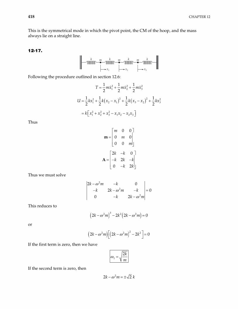
418 CHAPTER 12
This is the symmetrical mode in which the pivot point, the CM of the hoop, and the mass always lie on a straight line.
12-17.
kk m km km
x1 x2 x3 Following the procedure outlined in section 12.6:
2 21 2
1 1 12 2 2
T mx mx m 23x
222 21 2 1 3 2
2 2 21 2 3 1 2 2 3
1 1 1 12 2 2 2
U kx k x x k x x kx
k x x x x x x x
3
Thus
0 0
0 00 0
mm
mm
2 0
20 2
k kk k k
k kA
Thus we must solve
2
2
2
2 02 0
0 2
k m kk k m k
k k m
This reduces to
32 2 22 2 2k m k k m 0
or
22 2 22 2 2k m k m k 0
If the first term is zero, then we have
12km
If the second term is zero, then
22 2k m k
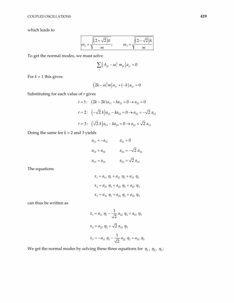
COUPLED OSCILLATIONS 419
which leads to
2 3
2 2 2 2;
k k
m m
To get the normal modes, we must solve
2 0jk r jk jrj
A m a
For k = 1 this gives:
21 22 0r r rk m a k a
Substituting for each value of r gives
11 21 21
12 22 22 12
13 23 23 13
1 : 2 2 0 0
2 : 2 0 2
3 : 2 0 2
r k k a ka a
a ka a
r k a ka a a
r k a
Doing the same for k = 2 and 3 yields
11 31 21
12 32 22 32
13 33 23 33
0
2
2
a a a
a a a a
a a a a
The equations
1 11 1 12 2 13
2 21 1 22 2 23
3 31 1 32 2 33
x a a a
x a a a
x a a a
3
3
3
can thus be written as
1 11 1 22 2 33 3
2 22 2 33 3
3 11 1 22 2 33
12
2
12
x a a a
x a a
x a a a 3
We get the normal modes by solving these three equations for 1 , 2 , 3 :

420 CHAPTER 12
1 31
11
1 22
22
2
22 2
x xa
x xa
3x
and
1 23
33
24
x xa
3x
The normal mode motion is as follows
1 1
2 2
3 2 1 3
:
: 2
: 2
x x
x x
x x x
3
1 32
2
x
12-18.
x1
y1m
b
x
MM
$
1 1
1 1
sin ; cos
cos ; sin
x x b x x b
y b b y b
Thus
2 2 21 1
2 2 2 2
1
1 12 2
1 12 cos
2 2
1 cos
T Mx m x y
Mx m x b b x
U mgy mgb
For small , 2
cos 12
. Substituting and neglecting the term of order 2 gives
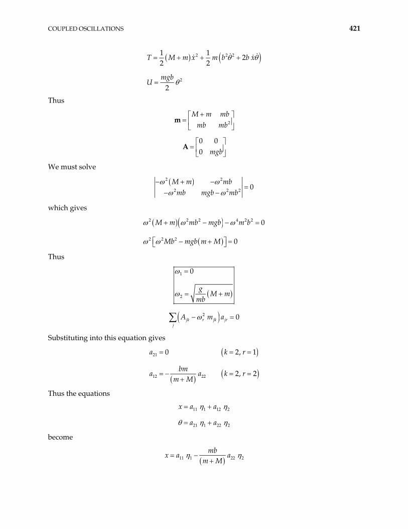
COUPLED OSCILLATIONS 421
2 2 2
2
1 12
2 2
2
T M m x m b b x
mgbU
Thus
2
M m mbmb mb
m
0 00 mgb
A
We must solve
2 2
2 2 0M m mb
mb mgb mb2
which gives
2 2 2 4 2
2 2 2
0
0
M m mb mgb m b
Mb mgb m M
2
Thus
1
2
0
gM m
mb
2 0jk r jk jrj
A m a
Substituting into this equation gives
21
12 22
0 2
2, 2
a k
bma a k
m M
, 1r
r
Thus the equations
11 1 12 2
21 1 22 2
x a a
a a
become
11 1 22 2mb
x a am M
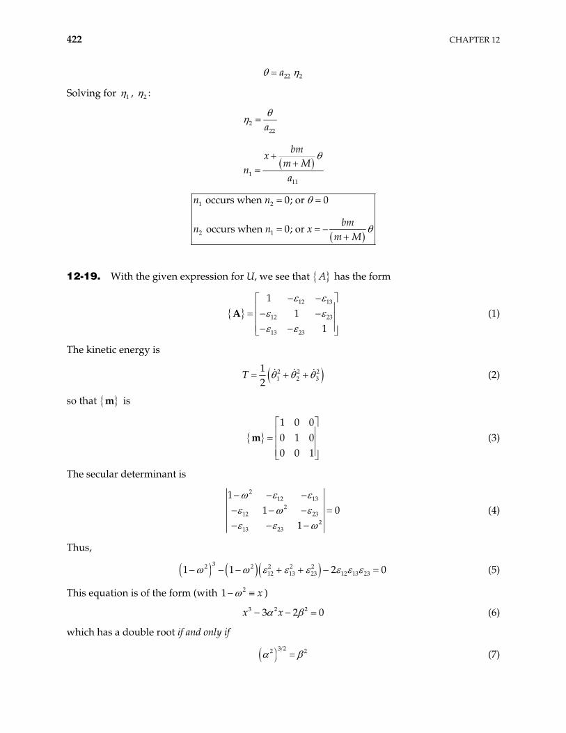
422 CHAPTER 12
22 2a
Solving for 1 , 2 :
222
111
a
bmx
m Mn
a
1 2
2 1
occurs when 0; or 0
occurs when 0; or
n n
bmn n x
m M
12-19. With the given expression for U, we see that A has the form
12 13
12 23
13 23
11
1A (1)
The kinetic energy is
2 2 21 2 3
12
T (2)
so that m is
1 0 00 1 00 0 1
m (3)
The secular determinant is
212 13
212 23
213 23
11
10 (4)
Thus,
32 2 2 2 2
12 13 23 12 13 231 1 2 0 (5)
This equation is of the form (with 1 2 x )
3 2 23 2x x 0 (6)
which has a double root if and only if
3 22 2 (7)
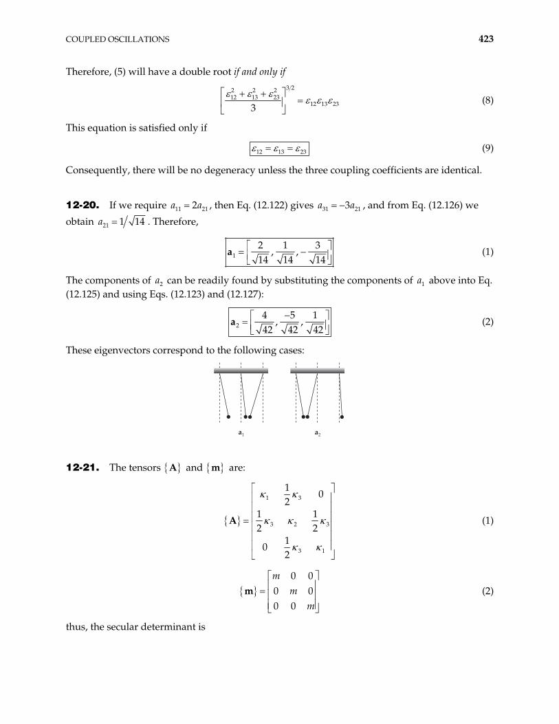
COUPLED OSCILLATIONS 423
Therefore, (5) will have a double root if and only if
3 22 2 2
12 13 2312 13 233
(8)
This equation is satisfied only if
12 13 23 (9)
Consequently, there will be no degeneracy unless the three coupling coefficients are identical.
12-20. If we require , then Eq. (12.122) gives 11 212a a 31 213a a , and from Eq. (12.126) we
obtain 21 1 14a . Therefore,
12 1 3
, ,14 14 14
a (1)
The components of can be readily found by substituting the components of above into Eq. (12.125) and using Eqs. (12.123) and (12.127):
2a 1a
24 5 1
, ,42 42 42
a (2)
These eigenvectors correspond to the following cases:
a1 a2
12-21. The tensors A and m are:
1 3
3 2 3
3 1
10
212 2
10
2
1A (1)
0 0
00 0
mm
m0m (2)
thus, the secular determinant is
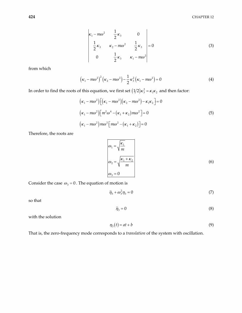
424 CHAPTER 12
21 3
23 2 3
23 1
10
21 1
02 2
10
2
m
m
m
(3)
from which
22 2 2 2
1 2 3 11
02
m m m (4)
In order to find the roots of this equation, we first set 23 11 2 2 and then factor:
(5)
2 2 21 1 2 1 2
2 2 4 21 1 2
2 2 21 1 2
0
0
0
m m m
m m m
m m m
Therefore, the roots are
11
1 22
3 0
m
m (6)
Consider the case 3 0 . The equation of motion is
23 3 3 0 (7)
so that
3 0 (8)
with the solution
3 t at b (9)
That is, the zero-frequency mode corresponds to a translation of the system with oscillation.
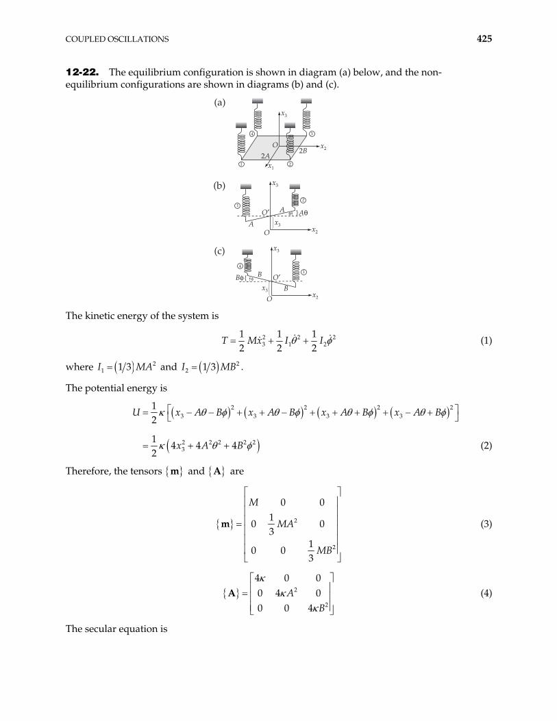
COUPLED OSCILLATIONS 425
12-22. The equilibrium configuration is shown in diagram (a) below, and the non-equilibrium configurations are shown in diagrams (b) and (c).
1 2
4 3
x1
x2
x3
O2A
2B
(a)
12
x3x
x3
O
O#A
A A$$
2
&'(
}
(b)
14
x3x
x3
O
O#B
BB% %
2
)*+
{
(c)
The kinetic energy of the system is
2 23 1 2
1 1 12 2 2
T Mx I I 2 (1)
where 21 1 3I MA and 2
2 1 3I MB .
The potential energy is
2 2 2 23 3 3 3
2 2 2 2 23
12
14 4 4
2
U x A B x A B x A B x A B
x A B (2)
Therefore, the tensors m and A are
2
2
0 01
03
10 0
3
M
MA 0
MB
m (3)
2
2
4 0 00 4 00 0 4
AB
A (4)
The secular equation is
426 CHAPTER 12
2 2 2 2 2 2 21 14 4 4
3 3M A MA B MB 0 (5)
Hence, the characteristic frequencies are
1
2
3 2
2
32
32
M
M
M
(6)
We see that 2 3 , so the system is degenerate.
The eigenvector components are found from the equation
2 0jk r jk jrj
A m a (7)
Setting to remove the indeterminacy, we find 32 0a
21 2 3
2
01 00 ; 3 ; 00 0 3
MMA
MB
aa a (8)
The normal coordinates are (for 3 0 0 0x 0 )
1 30 1
02
03 3
cos
cos3
cos3
t x M t
A Mt
B Mt t
2t (9)
Mode 1 corresponds to the simple vertical oscillations of the plate (without tipping). Mode 2 corresponds to rotational oscillations around the axis, and Mode 3 corresponds to rotational oscillations around the -axis.
1x
2x
The degeneracy of the system can be removed if the symmetry is broken. For example, if we place a bar of mass m and length 2A along the of the plate, then the moment of inertia around the is changed:
2 -axisx
1 -axisx
21
13
I M m A (10)
The new eigenfrequencies are
COUPLED OSCILLATIONS 427
1
2
3
2
32
32
M
M m
M
(11)
and there is no longer any degeneracy.
12-23. The total energy of the r-th normal mode is
2 21 1
2 2
r r r
r r
E T U
2r
(1)
where
ri tr re (2)
Thus,
ri tr r ri e (3)
In order to calculate T and U , we must take the squares of the real parts of r r r and r :
222
2
Re Re cos sin
cos sin
r r r r r r r
r r r r r r
i i t i
t t
t
(4)
so that
221
cos sin2r r r r r rT t t (5)
Also
222
2
Re Re cos sin
cos sin
r r r r r r
r r r r
i t i
t t
t
(6)
so that
221
cos2r r r r r rU t xin t (7)
Expanding the squares in T and U , and then adding, we find r r
428 CHAPTER 12
2 2 21
2
r r r
r r r
E T U
Thus,
2212r r rE (8)
So that the total energy associated with each normal mode is separately conserved.
For the case of Example 12.3, we have for Mode 1
1 10 20 cos2M
x x 1t (9)
Thus,
1 1 10 20 sin2M
x x 1t (10)
Therefore,
2 21 1 1
1 12 2
E 21 (11)
But
2 121
2M
(12)
so that
2 22 212 121 10 20 1 10 20
212 10 20
2 21 1sin cos
2 2 2 2
12
4
M ME x x t x x
M M
x x
1t
(13)
which is recognized as the value of the potential energy at t = 0. [At t = 0, , so that the total energy is
1 2 0x x
1 0U t .]
12-24. Refer to Fig. 12-9. If the particles move along the line of the string, the equation of motion of the j-th particle is
1j j j jmx x x x x 1j (1)
Rearranging, we find
1 2j j j jx x x xm 1 (2)
which is just Eq. (12.131) if we identify md with m .
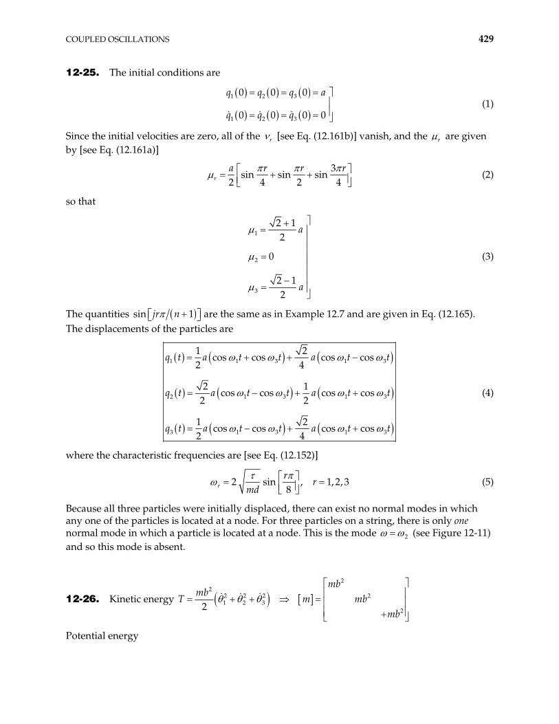
COUPLED OSCILLATIONS 429
12-25. The initial conditions are
1 2 3
1 2 3
0 0 0
0 0 0 0
q q q a
q q q (1)
Since the initial velocities are zero, all of the r [see Eq. (12.161b)] vanish, and the r are given by [see Eq. (12.161a)]
3
sin sin sin2 4 2 4ra r r r
(2)
so that
1
2
3
2 12
0
2 12
a
a
(3)
The quantities si are the same as in Example 12.7 and are given in Eq. (12.165). The displacements of the particles are
n 1jr n
1 1 3 1
2 1 3 1
3 1 3 1
1 2cos cos cos cos
2 4
2 1cos cos cos cos
2 2
1 2cos cos cos cos
2 4
q t a t t a t t
a t t a t t
q t a t t a t t
3
3
3
q t (4)
where the characteristic frequencies are [see Eq. (12.152)]
2 sin , 1, 28r
rr
md, 3 (5)
Because all three particles were initially displaced, there can exist no normal modes in which any one of the particles is located at a node. For three particles on a string, there is only one normal mode in which a particle is located at a node. This is the mode 2 (see Figure 12-11) and so this mode is absent.
12-26. Kinetic energy
22
2 2 2 21 2 3
22
mbmb
mbT m mb
Potential energy
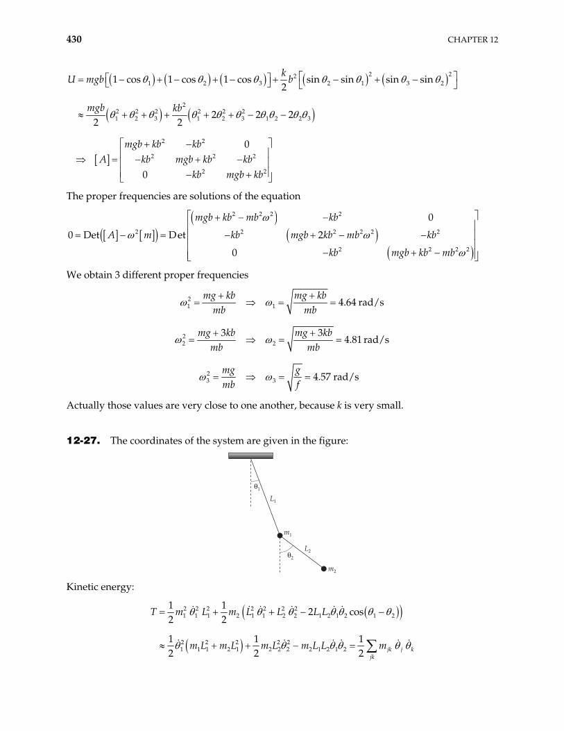
430 CHAPTER 12
2 221 2 3 2 1 3
22 2 2 2 2 21 2 3 1 2 3 1 2 2 3
2 2
2 2 2
2 2
1 cos 1 cos 1 cos sin sin sin sin2
2 2 22 2
0
0
kU mgb b
mgb kb
mgb kb kbA kb mgb kb kb
kb mgb kb
2
The proper frequencies are solutions of the equation
2 2 2 2
2 2 2 2 2
2 2
0
0 Det Det 2
0
mgb kb mb kb
A m kb mgb kb mb kb
kb mgb kb mb
2
2 2
We obtain 3 different proper frequencies
21 1
22 2
23 3
4.64 rad/s
3 34.81 rad/s
4.57 rad/s
mg kb mg kbmb mb
mg kb mg kbmb mb
mg gmb f
Actually those values are very close to one another, because k is very small.
12-27. The coordinates of the system are given in the figure:
L1
m1
m2
$1
$2
L2
Kinetic energy:
2 2 2 2 2 2 21 1 1 2 1 1 2 2 1 2 1 2 1 2
2 2 2 2 21 1 1 2 1 2 2 2 2 1 2 1 2
1 12 cos
2 2
1 1 12 2 2 jk j k
jk
T m L m L L L L
m L m L m L m L L m
COUPLED OSCILLATIONS 431
2
1 2 1 2 1 22
2 1 2 2 2jk
m m L m L Lm
m L L m L
Potential energy:
1 1 1 2 1 1 2 2
2 21 2
1 2 1 2 2
1 cos 1 cos 1 cos
12 2 2 jk j k
jk
U m gL m g L L
m m gL m gL A
1 2 1
2 2
00jk
m m gLA
m gL
Proper oscillation frequencies are solutions of the equation
2Det 0A m
2 221 2 1 2 1 2 1 1 2 2 1 2
1,21 1 22
m m g L L m m g m L L m L L
m L L
The eigenstate corresponding to 1 is 11
21
aa
where
1 2 1 1 221 112 221 2
1 2 1 2 1 2 1 1 2 2 1 2
21
m m L gm La a
m L m m g L L m m g m L L m L L
The eigenstate corresponding to 2 is 12
22
aa
where
1 2 1 1 222 122 221 2
1 2 1 2 1 2 1 1 2 2 1 2
21
m m L gm La a
m L m m g L L m m g m L L m L L
These expressions are rather complicated; we just need to note that and have the same
sign
11a 21a
11
21
0aa
while and have opposite sign 12a 22a 11
21
0aa
.
The relationship between coordinates 1 2, and normal coordinates 1 2, are
121 1
1 11 1 12 2 22
2 21 1 22 2 112 1
21
~
~
aa a aa a a
a
2
2
432 CHAPTER 12
To visualize the normal coordinate 1 , let 2 0 . Then to visualize the normal coordinate 2 ,
we let 1 0 . Because 11
21
0aa
and 12
22
aa
0 , we see that these normal coordinates describe two
oscillation modes. In the first one, the two bobs move in opposite directions and in the second, the two bobs move in the same direction.
12-28. Kinetic energy: 2
22 2 2 21 1 2 2 2
2
01 12 2 0
m bT m b m b m
m b
Potential energy: 1 1 2 2 1
2 21
2 22
1 cos 1 cos sin sin2k
U m gb m gb b b
m gb kb kbA
kb m gb kb
2
Solving the equation, 2Det 0A m , gives us the proper frequencies of oscillation,
2 21 25 (rad/s)
gb
2 22
1 2
25.11(rad/s)g k kb m m
The eigenstate corresponding to 1 is 11
22
aa
with 21 117.44a a
The eigenstate corresponding to 2 is 12
22
aa
with 22 128.55a a
From the solution of problem 12-27 above, we see that the normal coordinates are
121 1 2 1
22
~ 0aa 2.12
112 1 2 1
21
~ 0aa 2.13
Evidently 1 then characterizes the in-phase oscillation of two bobs, and 2 characterizes the out-of-phase oscillation of two bobs.
Now to incorporate the initial conditions, let us write the most general oscillation form:
1 1 2 2
1 1 2 2
1 1 2 2
1 11 12
2 21 22
11 12
Re
Re
Re 7.44 8.35
i t i i t i
i t i i t i
i t i i t i
a e a e
a e a e
a e a e
where is a real normalization constant. The initial conditions helps to determine parameters ’s, a’s, ’s.
COUPLED OSCILLATIONS 433
1 11 1 12 2
2 11 1 12
Re 0 7 cos cos 0.122 rad
Re 0 0 7.44 cos 8.35 cos 0
t a a
t a a 2
1 1sin sin 0 . Then
1 11 1 12 2 1 2
2 11 1 12 2 2
cos cos 0.065 cos 0.057 cos
7.44 cos 8.35 cos 0.48 cos cos
a t a t t
a t a t t 1t
where 1 5.03 rad/s , 2 4.98 rad/s (found earlier)
Approximately, the maximum angle 2 is 0.096 rad and it happens when
2
1
cos 1cos 1
tt
which gives
2 1
1 2
2 2 12 1 2
t n kt k n
because 1
2
101100
we finally find 50k n and 2
10063 st .
Note: 2 max 0.96 rad and at this value the small-angle approximation breaks down, and
the value 2max we found is just a rough estimate.

434 CHAPTER 12
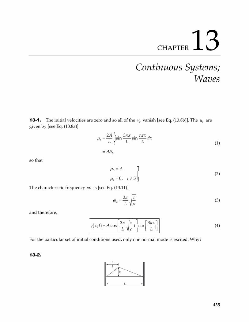
CHAPTER 13 Continuous Systems;
Waves
13-1. The initial velocities are zero and so all of the r vanish [see Eq. (13.8b)]. The r are given by [see Eq. (13.8a)]
0
3
2 3sin sin
L
r
r
A x r xdx
L L L
A
(1)
so that
3
0, 3r
A
r (2)
The characteristic frequency 3 is [see Eq. (13.11)]
33L
(3)
and therefore,
3 3
, cos sinx
q x t A tL L
(4)
For the particular set of initial conditions used, only one normal mode is excited. Why?
13-2.
L3
h
L
435
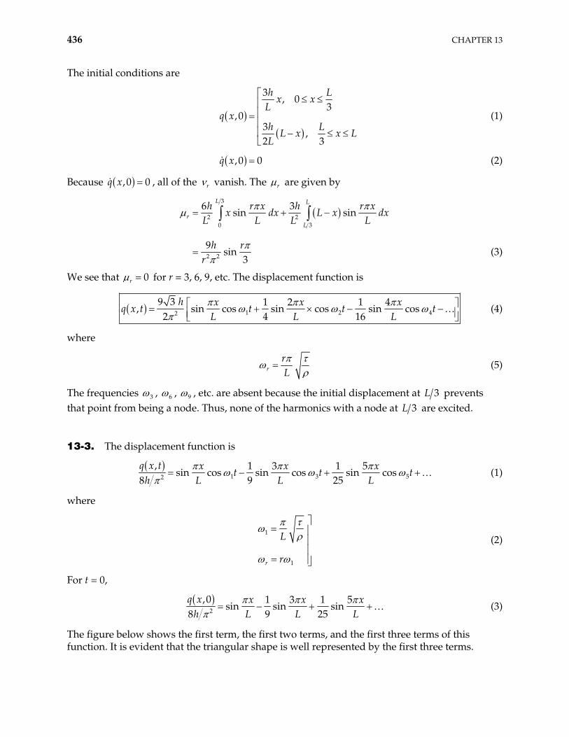
436 CHAPTER 13
The initial conditions are
3, 0
3,0
3,
2 3
h Lx x
Lq x
h LL x x L
L
(1)
,0 0q x (2)
Because ,0 0q x , all of the r vanish. The r are given by
3
2 20 3
2 2
6 3sin sin
9sin
3
L L
rL
h r x h r xx dx L x
L L L L
h rr
dx
(3)
We see that 0r for r = 3, 6, 9, etc. The displacement function is
1 22
9 3 1 2 1 4, sin cos sin cos sin cos
2 4 16h x x x
q x t t t tL L L 4 (4)
where
rrL
(5)
The frequencies 3 , 6 , 9 , etc. are absent because the initial displacement at 3L prevents that point from being a node. Thus, none of the harmonics with a node at 3L are excited.
13-3. The displacement function is
1 32
, 1 3 1 5sin cos sin cos sin cos
8 9 25q x t x x x
t th L L L 5t (1)
where
1
1r
L
r
(2)
For t = 0,
2
,0 1 3 1 5sin sin sin
8 9 25x x x
h L L Lq x
(3)
The figure below shows the first term, the first two terms, and the first three terms of this function. It is evident that the triangular shape is well represented by the first three terms.
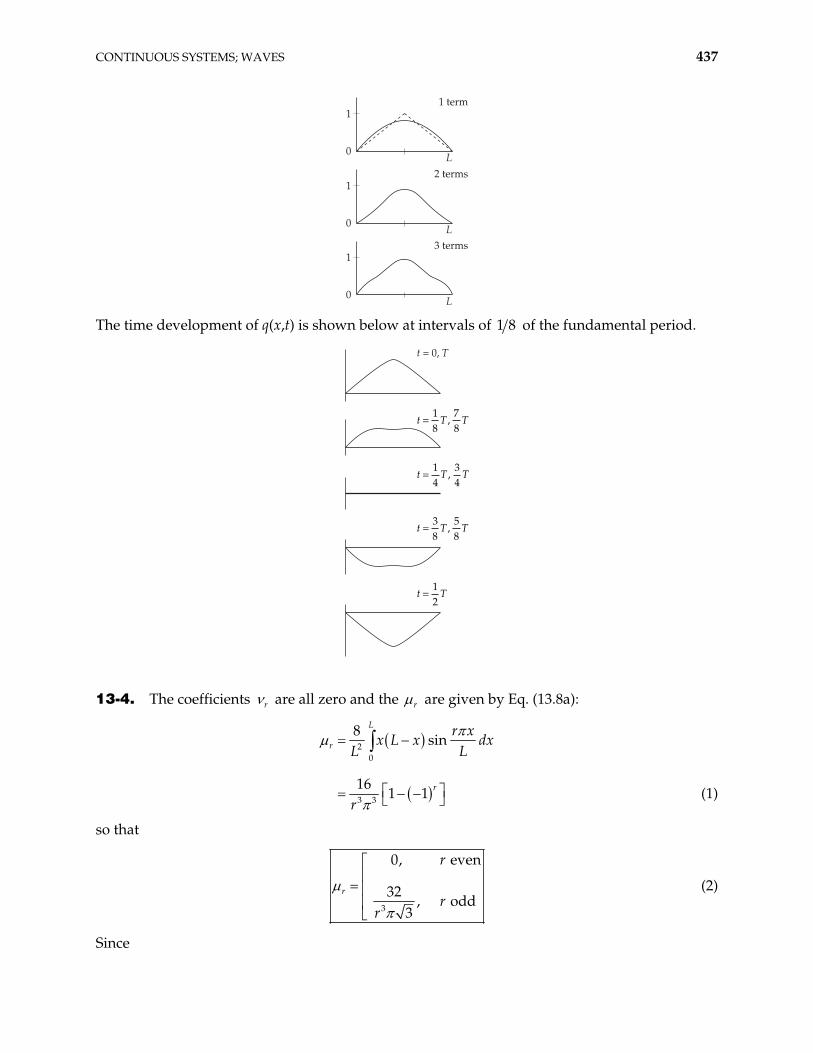
CONTINUOUS SYSTEMS; WAVES 437
1 term
L
1
0
2 terms
L
1
0
3 terms
L
1
0
The time development of q(x,t) is shown below at intervals of 1 of the fundamental period. 8
t = 0, T
t T= 18
78
, T
t T= 14
34
, T
t T= 38
58
, T
t T= 12
13-4. The coefficients r are all zero and the r are given by Eq. (13.8a):
20
3 3
8sin
161 1
L
r
r
r xx L x dx
L L
r (1)
so that
3
0, even
32, odd
3
r
r
rr
(2)
Since
438 CHAPTER 13
, sin cosrr
r xq x t t
L r (3)
the amplitude of the n-th mode is just n .
The characteristic frequencies are given by Eq. (13.11):
nnL
(4)
13-5. The initial conditions are
0
,0 0
1,
2,
0, otherwise
q x
v x sq x t
(1)
The r are all zero and the r are given by [see Eq. (13.8b)]
2
02
0
2sin
4sin sin
2
L s
rr L s
r
r xv d
L L
v r r sr L
x
(2)
from which
1 20
0, even
41 sin , od
r r
r
r
v r sr
r Ld
(3)
(Notice that the even modes are all missing, as expected from the symmetrical nature of the initial conditions.)
Now, from Eq. (13.11),
1 L (4)
and 1r r . Therefore,
1 202
1
41 sin , odr
rv r s
rr L
d (5)
According to Eq. (13.5),
CONTINUOUS SYSTEMS; WAVES 439
, sin
sin sin
ri tr
r
r rr
r xq x t e
L
r xt
L (6)
Therefore,
01 3
1
4 1 3 3, sin sin sin sin sin sin
9v s x s x
t t tL L L L
q x (7)
Notice that some of the odd modes—those for which sin 3 0s L —are absent.
13-6. The initial conditions are
0
0
,0 0
40
4
4,0
2 4
02
q x
v Lx x
L
v L Lq x x x
L
Lx L
2L (1)
The velocity at t = 0 along the string, ,0q x , is shown in the diagram.
v
L
v0
L4
L2
34L
The r are identically zero and the r are given by:
1 0
03 2
1
2,0 sin
8sin 2 sin
2 4
L
rr x
q x dxrL L
v rr
r (2)
Observe that for r = 4n, r is zero. This happens because at t = 0 the string was struck at 4L , and none of the harmonics with modes at that point can be excited.
Evaluation of the first few r gives
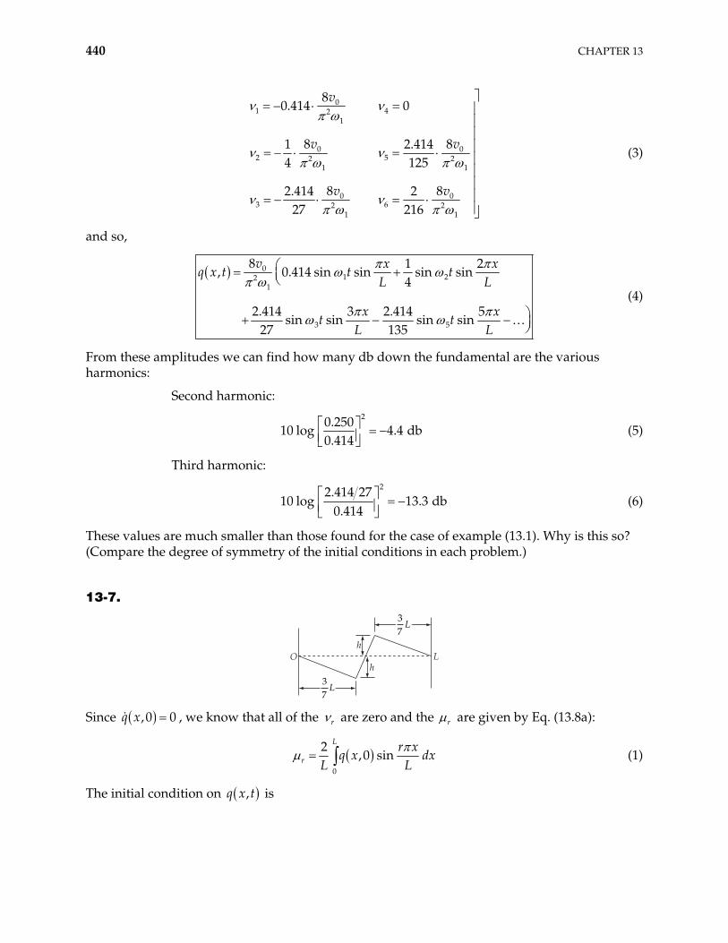
440 CHAPTER 13
01 42
1
02 52
1 1
0 03 62 2
1 1
80.414 0
81 2.414 125
8 82.414 227 216
v
v
v v
02
84 v (3)
and so,
01 22
1
3 5
8 1 2, 0.414 sin sin sin sin
4
2.414 3 2.414 5sin sin sin sin
27 135
v x xq x t t t
L L
x xt t
L L
(4)
From these amplitudes we can find how many db down the fundamental are the various harmonics:
Second harmonic:
20.250
10 log 4.4 db0.414
(5)
Third harmonic:
22.414 27
10 log 13.3 db0.414
(6)
These values are much smaller than those found for the case of example (13.1). Why is this so? (Compare the degree of symmetry of the initial conditions in each problem.)
13-7.
37
L
37
L
h
hLO
Since ,0 0q x , we know that all of the r are zero and the r are given by Eq. (13.8a):
0
2,0 sin
L
rr x
q x dxL L
(1)
The initial condition on ,q x t is
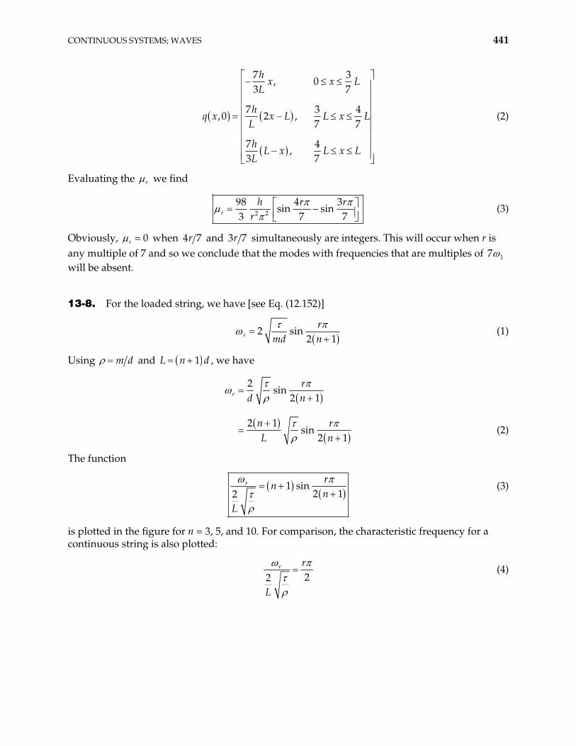
CONTINUOUS SYSTEMS; WAVES 441
7 3, 0
3 7
7 3,0 2 ,
7 7
7 4,
3 7
hx x
L
hx L L x L
L
hL x L x L
L
4
L
q x (2)
Evaluating the r we find
2 2
98 4 3sin sin
3 7rh r r
r 7 (3)
Obviously, 0r when 4 7r and 3 7r simultaneously are integers. This will occur when r is any multiple of 7 and so we conclude that the modes with frequencies that are multiples of 17 will be absent.
13-8. For the loaded string, we have [see Eq. (12.152)]
2 sin2 1r
rmd n
(1)
Using m d and 1L n d , we have
2sin
2 1
2 1sin
2 1
rr
d n
n rL n
(2)
The function
1 sin2 12
r rn
nL
(3)
is plotted in the figure for n = 3, 5, and 10. For comparison, the characteristic frequency for a continuous string is also plotted:
22
r r
L
(4)
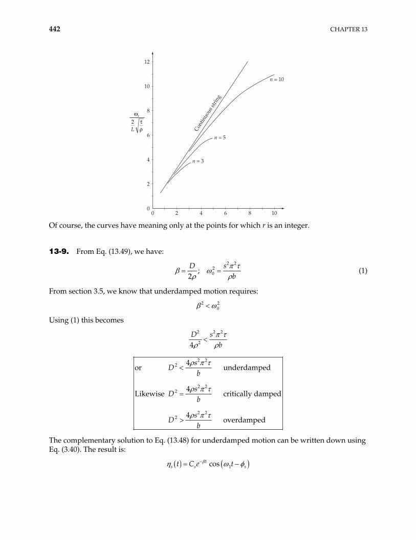
442 CHAPTER 13
00
2 4 6 8 10
2
4
6
8
10
12
Contin
uous
strin
g
n = 10
n = 5
n = 3
!"#
r
L2
Of course, the curves have meaning only at the points for which r is an integer.
13-9. From Eq. (13.49), we have:
2 2
20;
2D s
b (1)
From section 3.5, we know that underdamped motion requires:
2 20
Using (1) this becomes
2 2 2
24D s
b
2 22
2 22
2 22
4or underdamped
4ise critically damped
4overdamped
sD
b
sD
b
sD
b
Likew
The complementary solution to Eq. (13.48) for underdamped motion can be written down using Eq. (3.40). The result is:
1costs st C e t s
CONTINUOUS SYSTEMS; WAVES 443
where 2 21 0
2 , 0 and are as defined in (1), and C and s s are arbitrary constants depending on the initial conditions. The complete solution to Eq. (13.48) is the sum of the particular and complementary solutions (analogous to Eq. (13.50)):
0
1 2 22 2
2 sin cos2cos
st
s s s
sF t
t C e ts D
bb
where
12 2
2
tansD
sb
From Eq. (13.40):
, sinrr
r xq x t t
b
Thus
2 2 2 0
2 2 22 2
2 sin cos2, exp cos sin
2 4
(underdamped)
r
r rr
rF t
Dt s D r xq x t C t
b br Db
b
13-10. From Eq. (13.44) the equation for the driving Fourier coefficient is:
0
, sinb
ss x
f t F x t dxb
If the point x is a node for normal coordinate s, then
where is an integerx n
n sb s
(This comes from the fact that normal mode s has s-half wavelengths in length b.)
For x nb s
,
sin sin 0; hence 0ss x
n fb
t
444 CHAPTER 13
Thus, if the string is driven at an arbitrary point,
al modes with nodes at the driving point will be excited.none of the norm
13-11. From Eq. (13.44)
0
, sinb
ss x
f t F x t dxb
(1)
where ,F x t is the driving force, and sf t is the Fourier coefficient of the Fourier expansion of ,F x t . Eq. (13.45) shows that is the component of sf t ,F x t effective in driving normal
coordinate s. Thus, we desire ,F x t such that
0 for
0 for
sf t s n
s n
From the form of (1), we are led to try a solution of the form
, sinn x
F x t g tb
where g(t) is a function of t only.
Thus
0
sin sinb
sn x s x
f t g t dxb b
For n s, the integral is proportional to 0
sinb
x
n s xb
; hence 0sf t for s n.
For n = s, we have
2
0
sin 02
b
sn x b
f t g t dx g tb
Only the n normal coordinate will be driven. th
thThus, to drive the harmonic only,
, sin
nn x
F x t g tb
CONTINUOUS SYSTEMS; WAVES 445
13-12. The equation to be solved is
2 2
0s s sD s
b (1)
Compare this equation to Eq. (3.35):
202 0x x x
The solution to Eq. (3.35) is Eq. (3.37):
2 2 2 21 0 2exp expte A t A t0x t
Thus, by analogy, the solution to (1) is
2 22 2 2 2
21 22 2exp exp
4 4Dt
sD s D s
n t e A t A tb b
13-13. Assuming k is real, while and v are complex, the wave function becomes
, i t i t kx
t kx t
x t Ae
Ae e (1)
whose real part is
, costx t Ae t kx (2)
and the wave is damped in time, with damping coefficient .
From the relation
2
22k
v (3)
we obtain
(4) 2 22i k u iw
By equating the real and imaginary part of this equation we can solve for and in terms of u and w:
2k uw
(5)
and
(6) kw
iku
Since we have assumed to be real, we choose the solution
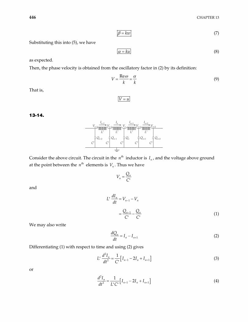
446 CHAPTER 13
kw (7)
Substituting this into (5), we have
ku (8)
as expected.
Then, the phase velocity is obtained from the oscillatory factor in (2) by its definition:
Re
Vk k
(9)
That is,
V u
13-14.
Vn+2Vn–2
L$
C$
InVn–1
L$
In+1Vn
L$
In+2Vn+1
Qn–1
C$Qn
C$Qn+1
C$Qn+2
C$Qn–2
L$
In–2
Consider the above circuit. The circuit in the inductor is I , and the voltage above ground at the point between the elements is V . Thus we have
thn nthn n
nn
QV
C
and
1
1
nn n
n
dIL V V
dt
Q QC C
n (1)
We may also write
1n
n ndQ
I Idt
(2)
Differentiating (1) with respect to time and using (2) gives
2
12
12n
n n nd I
L I Idt C 1I (3)
or
2
12
12n
n n nd I
I I Idt L C 1 (4)
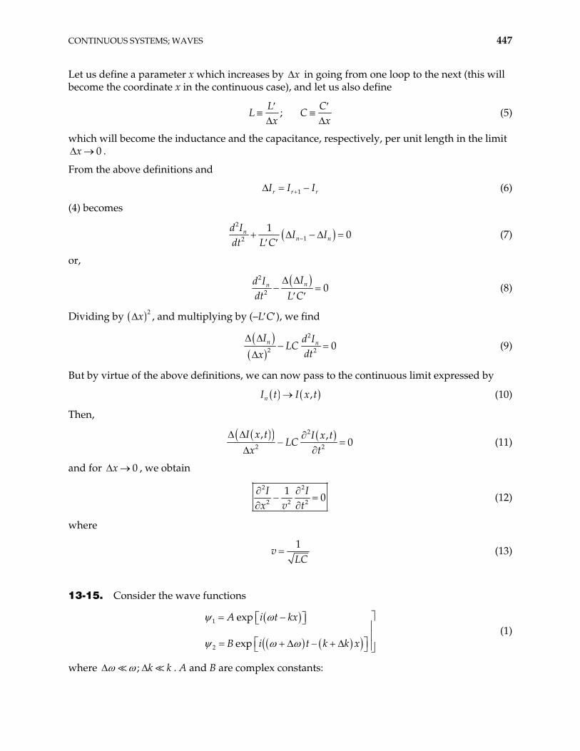
CONTINUOUS SYSTEMS; WAVES 447
Let us define a parameter x which increases by x in going from one loop to the next (this will become the coordinate x in the continuous case), and let us also define
;L C
L Cx x
(5)
which will become the inductance and the capacitance, respectively, per unit length in the limit . 0x
From the above definitions and
1r rI I Ir (6)
(4) becomes
2
12
10n
n nd I
I Idt L C
(7)
or,
2
2 0nn Id Idt L C
(8)
Dividing by 2x , and multiplying by (–L C ), we find
2
2 2 0n nI d ILC
dtx (9)
But by virtue of the above definitions, we can now pass to the continuous limit expressed by
,nI t I x t (10)
Then,
2
2 2
, ,0
I x t I x tLC
x t (11)
and for , we obtain 0x
2 2
2 2 2
10
I Ix v t
(12)
where
1
vLC
(13)
13-15. Consider the wave functions
1
2
exp
exp
A i t kx
B i t k k x (1)
where ; k k . A and B are complex constants:
448 CHAPTER 13
exp
exp
a
b
A A i
B B i (2)
The superposition of 1 and 2 is given by
1 2
2 2exp exp exp2 2
t kx t kxi
a bk
i t k x A i e B i ei (3)
which can be rewritten as
2exp2 2 2
a b b at kx t kxi i
a bki w t k x A e B e 2 (4)
Define
b a
t x k (5)
and
2 2i i iA e B e e (6)
Therefore,
2 22 2A B (7)
1 22 2cos cos
22
aA B
A B (8)
1 22 2sin sin
22
aB A
A B (9)
That is, is a function of t k x . Using (6) and (7) – (9), we can rewrite (4) as
exp2 2 2
ia bki t k x e (10)
and then,
Re cos cos2 2 2
sin sin2 2 2
a b
a b
kt k x
kt k x
(11)
CONTINUOUS SYSTEMS; WAVES 449
From this expression we see that the wave function is modulated and that the phenomenon of beats occurs, but for A B, the waves never beat to zero amplitude; the minimum amplitude is, from Eq. (11), A B , and the maximum amplitude is A B . The wave function has the form shown in the figure.
A B+ A B%Re&
wt – kx
13-16. As explained at the end of section 13.6, the wave will be reflected at and will then propagate in the –x direction.
0x x
13-17. We let
, 2
, 2j
m j nm
m j n 1 (1)
where n is an integer.
Following the procedure in Section 12.9, we write
2 2 2 1 2 22n n n n nF m q q q qd 1 (2a)
2 1 2 1 2 2 1 2 22n n n nF m q q q qd n (2b)
Assume solutions of the form
22
i t nkdnq Ae (3a)
2 12 1
i t n kdnq Be (3b)
Substituting (3a,b) into (2a,b), we obtain
2
2
2
2
ikd ikd
ikd ikd
A Be A Bem d
B Ae B Aem d
(4)
from which we can write
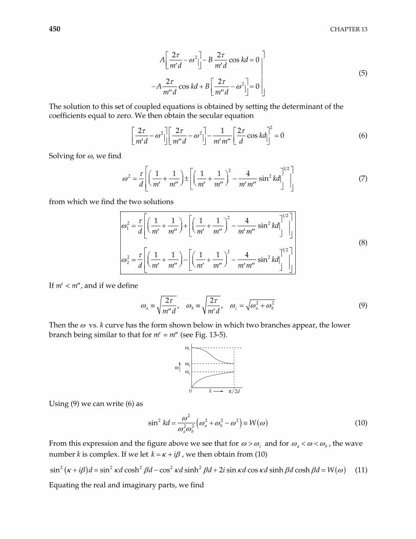
450 CHAPTER 13
2
2
2 2cos 0
2 2cos 0
A B kdm d m d
A kd Bm d m d
(5)
The solution to this set of coupled equations is obtained by setting the determinant of the coefficients equal to zero. We then obtain the secular equation
2
2 22 2 1 2cos 0kd
m d m d m m d (6)
Solving for , we find
1 221 1 1 1 4
sin kdd m m m m m m
2 2 (7)
from which we find the two solutions
1 222 21
1 222 22
1 1 1 1 4sin
1 1 1 1 4sin
kdd m m m m m m
kdd m m m m m m
(8)
If m < m , and if we define
22 2, ,a b cm d m d
2a b (9)
Then the vs. k curve has the form shown below in which two branches appear, the lower branch being similar to that for m = m (see Fig. 13-5).
!a
!b
!c
0 k
!
'/2d Using (9) we can write (6) as
2
2 2 2 22 2sin a ba b
kd W (10)
From this expression and the figure above we see that for c and for a b , the wave number k is complex. If we let , we then obtain from (10) k i
2 2 2 2 2sin sin cosh cos sinh 2 sin cos sinh coshi d d d d d i d d d d W (11)
Equating the real and imaginary parts, we find
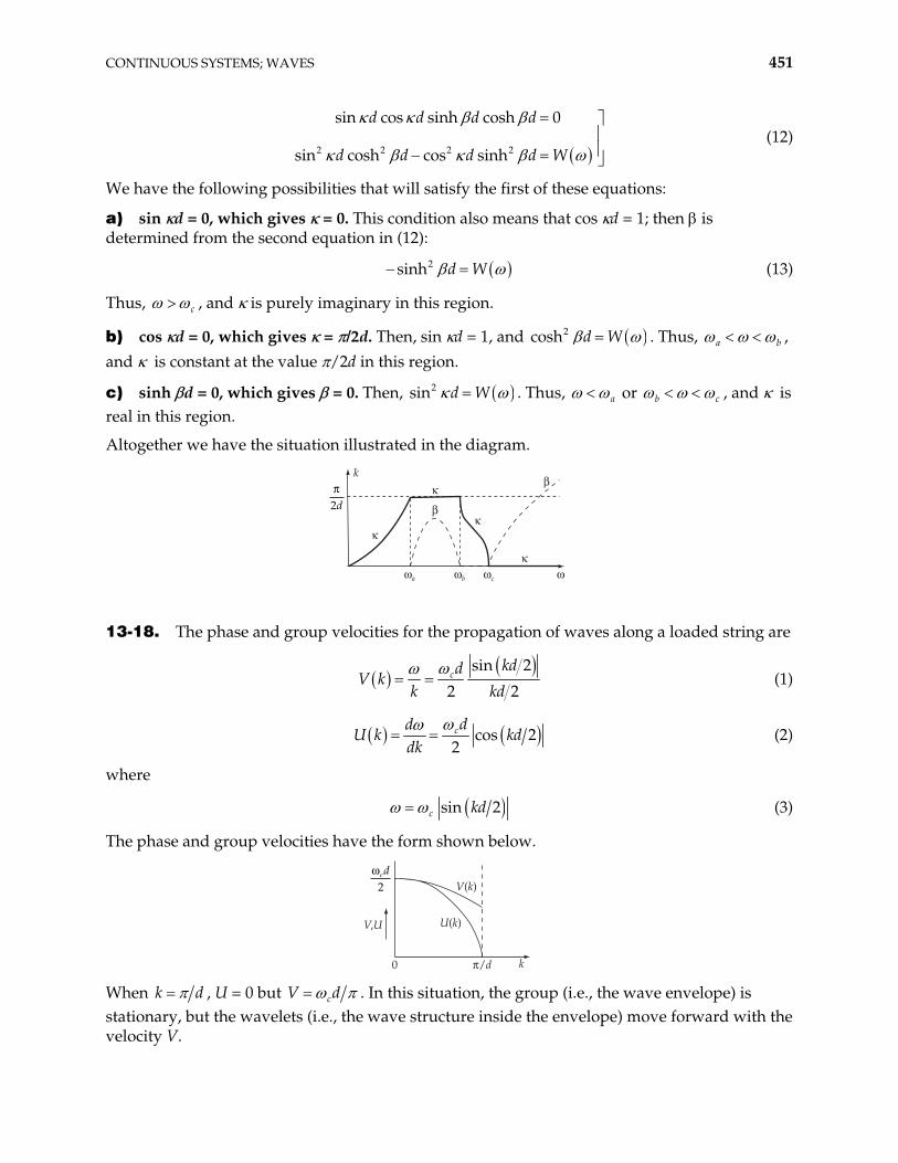
CONTINUOUS SYSTEMS; WAVES 451
2 2 2 2
sin cos sinh cosh 0
sin cosh cos sinh
d d d d
d d d d W (12)
We have the following possibilities that will satisfy the first of these equations:
a) sin d = 0, which gives = 0. This condition also means that cos d = 1; then is determined from the second equation in (12):
2sinh d W (13)
Thus, c , and is purely imaginary in this region.
b) cos d = 0, which gives = /2d. Then, sin d = 1, and 2cosh d W . Thus, a b , and is constant at the value /2d in this region.
c) sinh d = 0, which gives = 0. Then, 2n d Wsi . Thus, a or b c , and is real in this region.
Altogether we have the situation illustrated in the diagram.
k
(
(
(
(!a !b !c !
)
)'2d
13-18. The phase and group velocities for the propagation of waves along a loaded string are
sin 2
2 2c
kddV k
k kd (1)
cos 22cdd
U k kddk
(2)
where
sin 2c kd (3)
The phase and group velocities have the form shown below.
V,U U(k)
V(k)
0 k'/d
!cd2
When k d , U = 0 but cdV . In this situation, the group (i.e., the wave envelope) is stationary, but the wavelets (i.e., the wave structure inside the envelope) move forward with the velocity V.
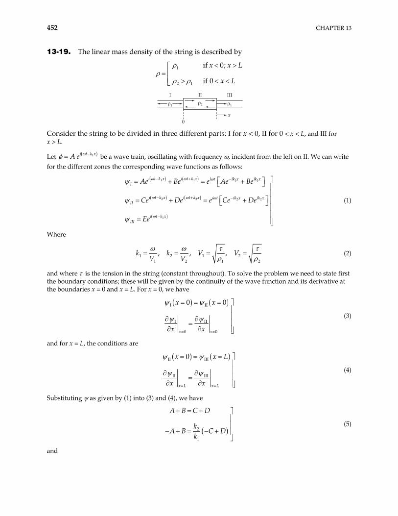
452 CHAPTER 13
13-19. The linear mass density of the string is described by
1
2 1
if 0;
if 0
x x
x L
L
I II III
0x
#1 #1#2
Consider the string to be divided in three different parts: I for x < 0, II for 0 < x < L, and III for x > L.
Let be a wave train, oscillating with frequency , incident from the left on II. We can write for the different zones the corresponding wave functions as follows:
1i t k xA e
II
1 1 1 1
2 2 2 2
1
i t k x i t k x i t ik x ik xI
i t k x i t k x i t ik x ik x
i t k xIII
Ae Be e Ae Be
Ce De e Ce De
Ee
(1)
Where
1 2 1 21 2 1
, , ,V VV V 2
k k (2)
and where is the tension in the string (constant throughout). To solve the problem we need to state first the boundary conditions; these will be given by the continuity of the wave function and its derivative at the boundaries x = 0 and x = L. For x = 0, we have
I II
I II
0 0
0 0
x x
x x
x x
(3)
and for x = L, the conditions are
II III
II III
0
x L x L
x x
x x
L
(4)
Substituting as given by (1) into (3) and (4), we have
2
1
A B C D
kA B C D
k
(5)
and
CONTINUOUS SYSTEMS; WAVES 453
2 2 1
2 2 11
2
ik L ik L ik L
ik L ik L ik L
C e D e E e
kC e D e E e
k
(6)
From (6) we obtain
2 1
2 1
1
2
1
2
11
2
11
2
i k k L
i k k L
kC E e
k
kD E e
k
(7)
Hence,
222 1
2 1
i k Lk kC e
k kD (8)
From (5) we have
2
1 1
1 11 1
2 2k k2A Ck k
D (9)
Using (7) and rearranging the above equation
2
21 2 2
2 11 2 1
12
i k Lk kA e k k
k k kD (10)
In the same way
222 1 1 2
1
12
i k LB k k e k kk
D (11)
From (10) and (11) we obtain
2
2
2 2 21 2
2 21 2 1 2
1i k L
i k L
k k eBA k k e k k 2 (12)
On the other hand, from (6) and (8) we have
2 12
2 1
2 i k k Lk DE e
k k (13)
which, together with (10) gives
1 2
2
1 22 2
1 2 1 2
4 i k k L
i k L
k k eEA k k e k k 2 (14)
Since the incident intensity is proportional to 0I 2A , the reflected intensity is 2rI B , and the total
transmitted intensity is 2t EI , we can write
454 CHAPTER 13
2 2
0 2 ,r tB E
I I I I0 2A A (15)
Substituting (12) and (14) into (15), we have, for the reflected intensity,
2
2
22 2 21 2
0 2 21 2 1 2
1i k L
r i k L
k k eI I
k k e k k 2 (16)
From which
22 21 2 2
0 24 4 2 2 2 21 2 1 2 1 2 2
1 cos 2
6 cos 2r
k k k L
k k k k k k k LI I (17)
and for the transmitted intensity, we have
1 2
2
2
1 20 2 2
1 2 1 2
4 i k k L
t i k L
k k eI I
k k e k k 2 (18)
so that
2 21 2
0 24 4 2 2 2 21 2 1 2 1 2 2
8
6 2 cos 2t
k k
k k k k k k k LI I (19)
We observe that I I , as it must. 0r t I
For maximum transmission we need minimum reflection; that is, the case of best possible transmission is that in which
0
0
t
r
I I
I (20)
In order that , (17) shows that L must satisfy the requirement 0rI
21 cos 2 0k L (21)
so that we have
2 2
, 0,1, 2,m m
L mk
(22)
The optical analog to the reflection and transmission of waves on a string is the behavior of light waves which are incident on a medium that consists of two parts of different optical densities (i.e., different indices of refraction). If a lens is given a coating of precisely the correct thickness of a material with the proper index of refraction, there will be almost no reflected wave.
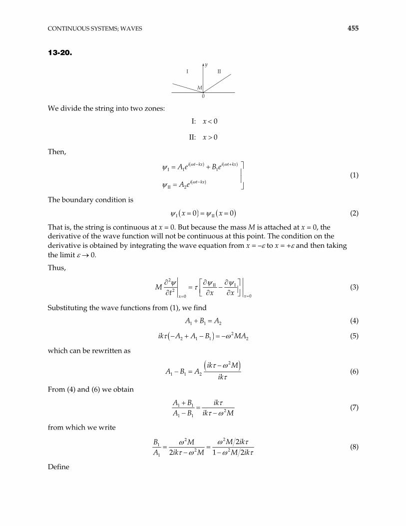
CONTINUOUS SYSTEMS; WAVES 455
13-20.
I II
M
0
y
We divide the string into two zones:
I: 0
II: 0
x
x
Then,
I 1 1
II 2
i t kx i t kx
i t kx
A e B e
A e (1)
The boundary condition is
I II0x x 0 (2)
That is, the string is continuous at x = 0. But because the mass M is attached at x = 0, the derivative of the wave function will not be continuous at this point. The condition on the derivative is obtained by integrating the wave equation from x = – to x = + and then taking the limit 0.
Thus,
2
II I2
00 xx
Mt x x
2
(3)
Substituting the wave functions from (1), we find
1 1A B A (4)
22 1 1ik A A B MA2 (5)
which can be rewritten as
2
1 1 2
ik MA B A
ik (6)
From (4) and (6) we obtain
1 12
1 1
A B ikA B ik M
(7)
from which we write
22
12 2
1
22 1 2
M ikB MA ik M M ik
(8)
Define
456 CHAPTER 13
2
tan2
MP
k (9)
Then, we can rewrite (8) as
1
1 1B iPA iP
(10)
And if we substitute this result in (4), we obtain a relation between 1A and 2A :
2
1
11
AA iP
(11)
The reflection coefficient, 2
1
1
BR
A, will be, from (10),
2 22
12
1
tan1 1 tan
B PR
A P 2 (12)
or,
2sinR (13)
and the transmission coefficient, 2
2
1
AT
A, will be from (10)
2
22
1
1 11 1 tan
AT
A P 2 (14)
or,
2cosT (15)
The phase changes for the reflected and transmitted waves can be calculated directly from (10) and (11) if we substitute
1 1 1
1 1 1
2 2 2
i
i
i
B B e B
A A e A
A A e A
(16)
Then,
1
1 1 tan 1112
1 1 1Ai iBB P
eA A P
B Pe (17)
and
1
2 12 tan22
1 1
1
1A Ai iAA
eA A P
Pe (18)
CONTINUOUS SYSTEMS; WAVES 457
Hence, the phase changes are
1 1
2 1
1 1
1 1
1tan tan cot
tan tan tan
B A
A A
P
P
(19)
13-21. The wave function can be written as {see Eq. (13.111a)]
(1) , i t kxx t A k e dk
Since A(k) has a non-vanishing value only in the vicinity of 0k k , (1) becomes
(2) 0
0
,k k
i t kx
k k
x t e dk
According to Eq. (13.113),
0 0 0k k (3)
Therefore, (2) can now be expressed as
0
0 0 0 0
0
0 0 0 00 0 0
0 0 0 0 0
0
0
,
22
k ki w k t i t x k
k k
i k k t x i k k t xi k t
i k t i t x k i t x k
x t e e dk
e ee
i t x
e e et x i
(4)
and writing the term in the brackets as a sine, we have
0 00
0
2 sin, i t k xt x k
x t et x
(5)
The real part of the wave function at t = 0 is
02 sin
Re ,0 cosx k
xx
k x (6)
If , the cosine term will undergo many oscillations in one period of the sine term. That is, the sine term plays the role of a slowly varying amplitude and we have the situation in the figure below.
0k k
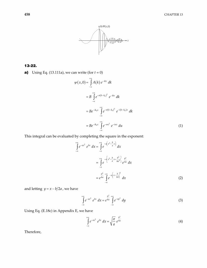
458 CHAPTER 13
x
Re*(x,0)
13-22.
a) Using Eq. (13.111a), we can write (for t = 0)
(1)
20
20 00
20
,0 ikx
k k ikx
k k i k k xik x
ik x u iux
x A k e dk
B e e dk
Be e e dk
Be e e du
This integral can be evaluated by completing the square in the exponent:
22
2 222
22
4 4
24
ba x xax bx a
b b ba x xa a a
bb a xaa
e e dx e dx
e e
e e dx
dx
(2)
and letting 2y x b a , we have
2
224b
ayax bx ae e dx e e dy (3)
Using Eq. (E.18c) in Appendix E, we have
2
24b
ax bx ae e dx ea
(4)
Therefore,
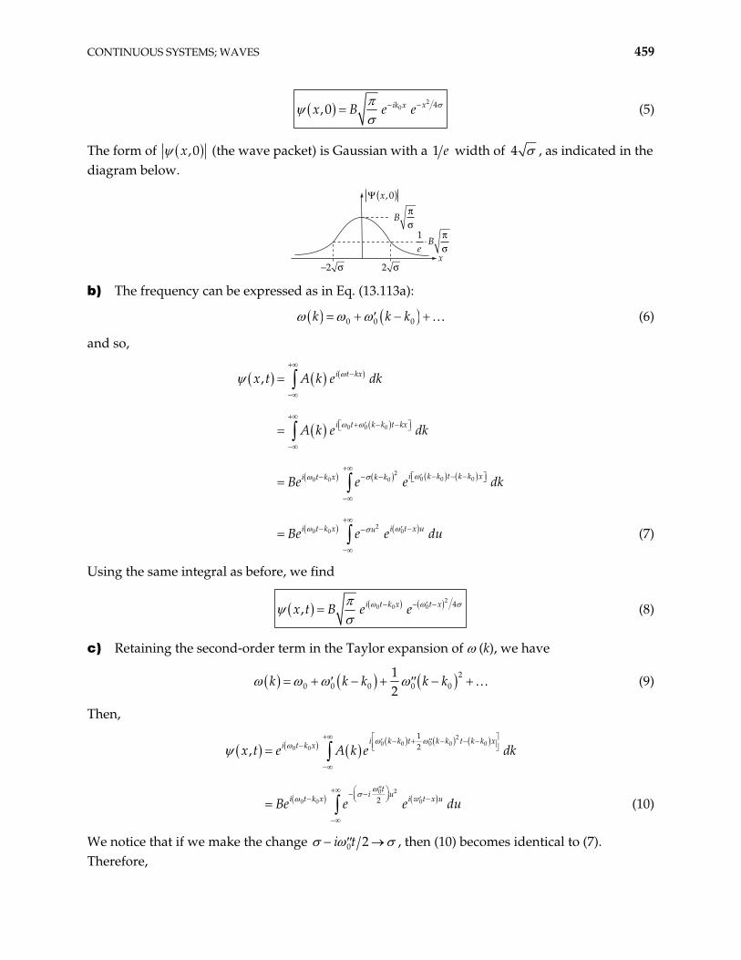
CONTINUOUS SYSTEMS; WAVES 459
2
0 4,0 xik xx B e e (5)
The form of ,0x (the wave packet) is Gaussian with a 1 width of e 4 , as indicated in the diagram below.
%2 + 2 +
1e
, B'+
B'+
* x, 0( )
x
b) The frequency can be expressed as in Eq. (13.113a):
0 0 0k k k (6)
and so,
(7)
0 0 0
20 0 00 0 0
20 0 0
, i t kx
i t k k t kx
i k k t k k xi t k x k k
i t k x i t x uu
x t A k e dk
A k e dk
Be e e dk
Be e e du
Using the same integral as before, we find
2
0 0 0 4, i t k x t xx t B e e (8)
c) Retaining the second-order term in the Taylor expansion of (k), we have
20 0 0 0 0
12
k k k k k (9)
Then,
20 0 0 0 0
0 0
20
0 0 0
12
2
,i k k t k k t k k xi t k x
ti ui t k x i w t x u
x t e A k e dk
Be e e du (10)
We notice that if we make the change 0 2i t , then (10) becomes identical to (7). Therefore,
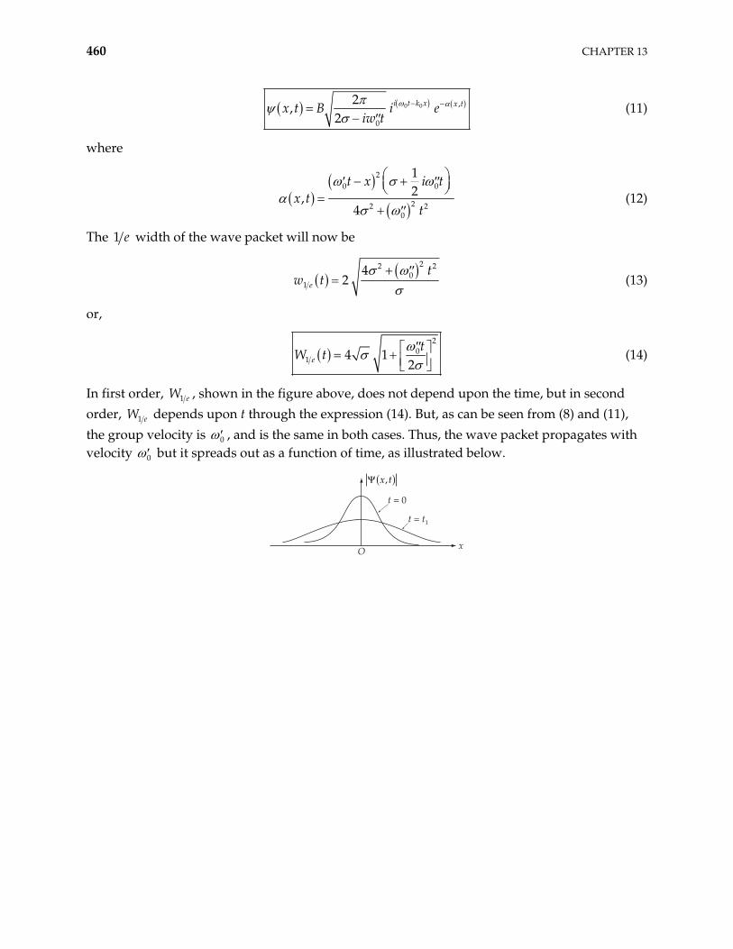
460 CHAPTER 13
0 0 ,
0
2,
2i t k x x tx t B i e
iw t (11)
where
20 0
22 20
12,
4
t x i tx t
t (12)
The 1 width of the wave packet will now be e
22 2
01
42e
tw t (13)
or,
2
01 4 1
2et
W t (14)
In first order, 1 eW , shown in the figure above, does not depend upon the time, but in second order, 1 eW depends upon t through the expression (14). But, as can be seen from (8) and (11), the group velocity is 0 , and is the same in both cases. Thus, the wave packet propagates with velocity 0 but it spreads out as a function of time, as illustrated below.
O x
t = t1
t = 0
* x t,( )
CHAPTER 14 The Special Theory
of Relativity
14-1. Substitute Eq. (14.12) into Eqs. (14.9) and (14.10):
1 1v
x x xc 1 (1)
1 1 1v
x x xc
(2)
From (1)
1
1
1x vx c
From (2)
1
1
1
1
xvxc
So
1
11
vvcc
or
2 2
1
1 v c
461
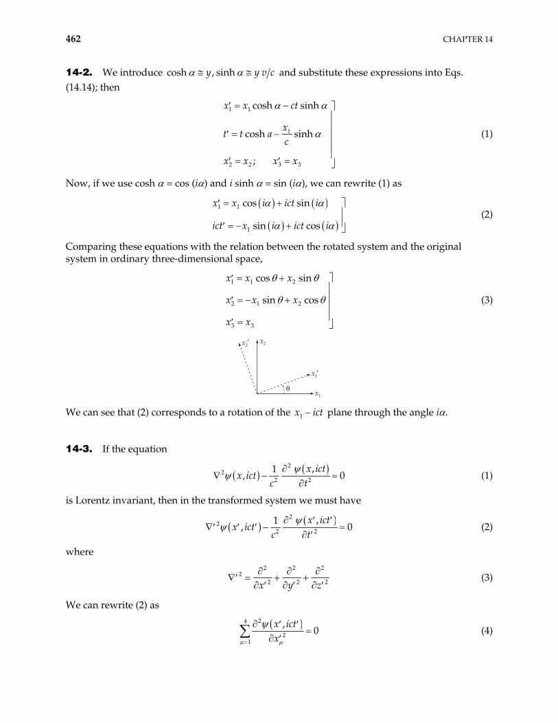
462 CHAPTER 14
14-2. We introduce cosh , sinhy y v c and substitute these expressions into Eqs. (14.14); then
1 1
1
2 2 3 3
cosh sinh
cosh sinh
;
x x ct
xt t a
c
x x x x
(1)
Now, if we use cosh = cos (i ) and i sinh = sin (i ), we can rewrite (1) as
1 1
1
cos sin
sin cos
x x i ict i
ict x i ict i (2)
Comparing these equations with the relation between the rotated system and the original system in ordinary three-dimensional space,
1 1 2
2 1 2
3 3
cos sin
sin cos
x x x
x x x
x x
(3)
x2x2!
x1
x1!
"
We can see that (2) corresponds to a rotation of the 1x ict plane through the angle i .
14-3. If the equation
2
22 2
,1,
x ictx ict
c t0 (1)
is Lorentz invariant, then in the transformed system we must have
2
22 2
,1,
x ictx ict
c t0 (2)
where
2 2
22 2x y z
2
2 (3)
We can rewrite (2) as
24
21
,0
x ictx
(4)
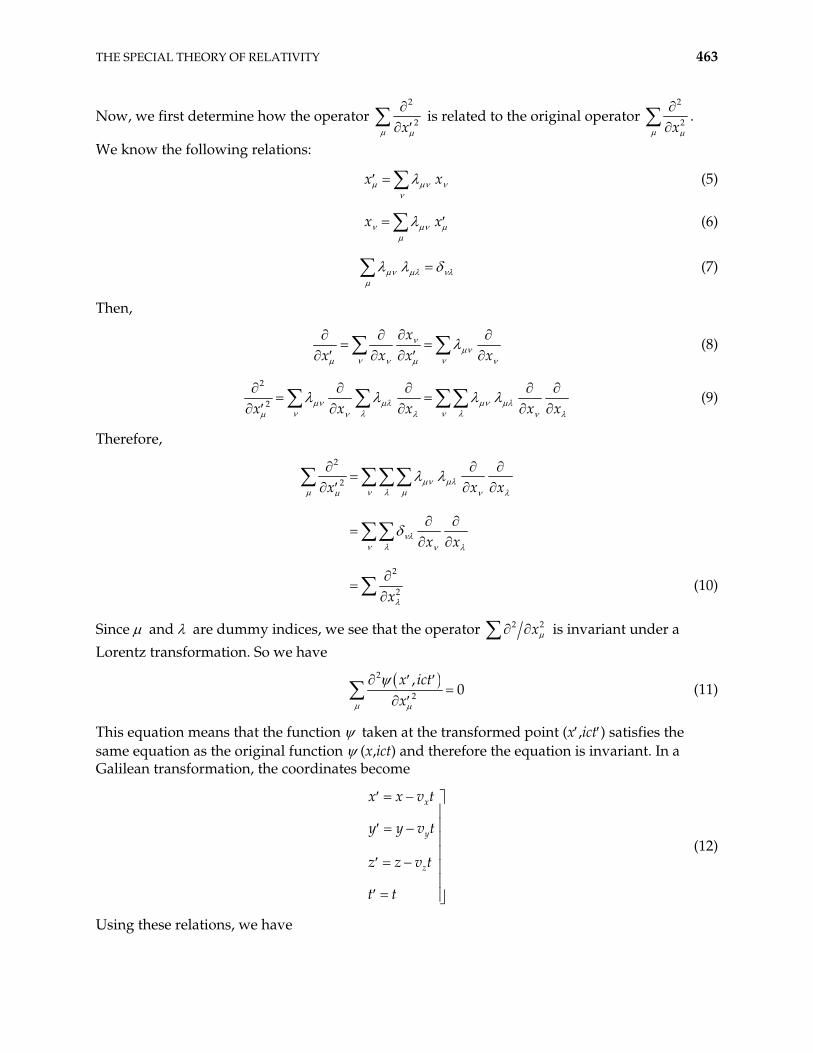
THE SPECIAL THEORY OF RELATIVITY 463
Now, we first determine how the operator 2
2x is related to the original operator
2
2x.
We know the following relations:
x x (5)
x x (6)
(7)
Then,
x
x x x x (8)
2
2x x x x x (9)
Therefore,
2
2
2
2
x x
x x
x
x
(10)
Since and are dummy indices, we see that the operator 2 x2 is invariant under a Lorentz transformation. So we have
2
2
,0
x ictx
(11)
This equation means that the function taken at the transformed point (x ,ict ) satisfies the same equation as the original function (x,ict) and therefore the equation is invariant. In a Galilean transformation, the coordinates become
x
y
z
x x v t
y y v t
z z v t
t t
(12)
Using these relations, we have
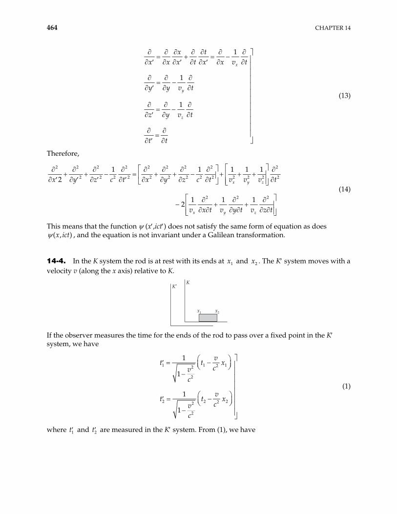
464 CHAPTER 14
1
1
1
x
y
z
x tx x x t x x v t
y y v t
z y v t
t t
(13)
Therefore,
2 2 2 2 2 2 2 2
2 2 2 2 2 2 2 2 2 2 2 2
2 2 2
1 1 1 1 12
1 1 12
x y z
x y z
x y z c t x y z c t v v v t
v x t v y t v z t
2
2
(14)
This means that the function (x ,ict ) does not satisfy the same form of equation as does ( , )x ict , and the equation is not invariant under a Galilean transformation.
14-4. In the K system the rod is at rest with its ends at and . The K system moves with a velocity v (along the x axis) relative to K.
1x 2x
KK!
x1 x2
If the observer measures the time for the ends of the rod to pass over a fixed point in the K system, we have
1 1 22
2
2 2 22
2
1
1
1
1
vt t
cvc
vt t
cvc
1
2
x
x
(1)
where t and t are measured in the K system. From (1), we have 1 2
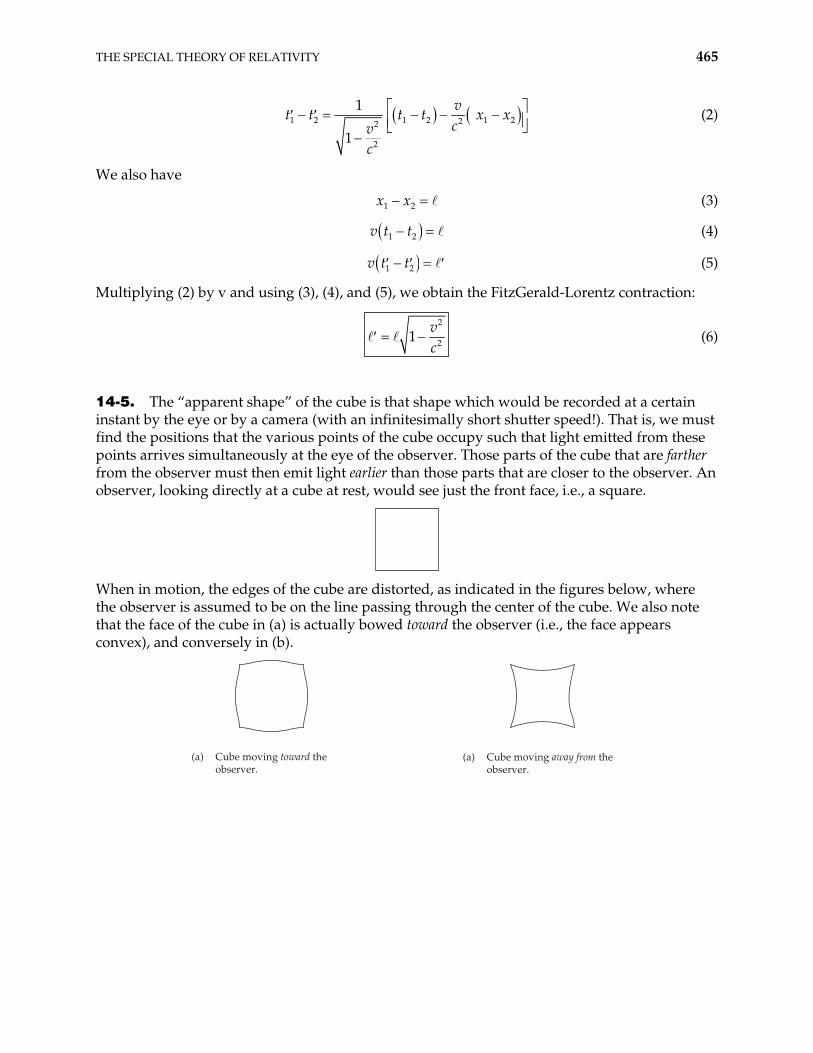
THE SPECIAL THEORY OF RELATIVITY 465
1 2 1 2 1 222
2
1
1
vt t x x
cvc
t t (2)
We also have
1 2x x (3)
1 2v t t (4)
1 2v t t (5)
Multiplying (2) by v and using (3), (4), and (5), we obtain the FitzGerald-Lorentz contraction:
2
21vc
(6)
14-5. The “apparent shape” of the cube is that shape which would be recorded at a certain instant by the eye or by a camera (with an infinitesimally short shutter speed!). That is, we must find the positions that the various points of the cube occupy such that light emitted from these points arrives simultaneously at the eye of the observer. Those parts of the cube that are farther from the observer must then emit light earlier than those parts that are closer to the observer. An observer, looking directly at a cube at rest, would see just the front face, i.e., a square.
When in motion, the edges of the cube are distorted, as indicated in the figures below, where the observer is assumed to be on the line passing through the center of the cube. We also note that the face of the cube in (a) is actually bowed toward the observer (i.e., the face appears convex), and conversely in (b).
(a) Cube moving toward the
observer. (a) Cube moving away from the
observer.
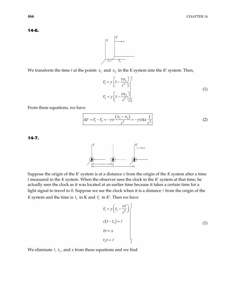
466 CHAPTER 14
14-6.
K!v
x1 x2
K
We transform the time t at the points and in the K system into the K system. Then, 1x 2x
11 2
22 2
vxt t
c
vxt t
c
(1)
From these equations, we have
1 21 2 2
1x xt t t v v x
c c2 (2)
14-7.
K K!v
x Suppose the origin of the K system is at a distance x from the origin of the K system after a time t measured in the K system. When the observer sees the clock in the K system at that time, he actually sees the clock as it was located at an earlier time because it takes a certain time for a light signal to travel to 0. Suppose we see the clock when it is a distance from the origin of the K system and the time is t in K and 1 1t in K . Then we have
1 1 2
1
1
vt t
c
c t t
tv x
t v
(1)
We eliminate , t , and x from these equations and we find 1
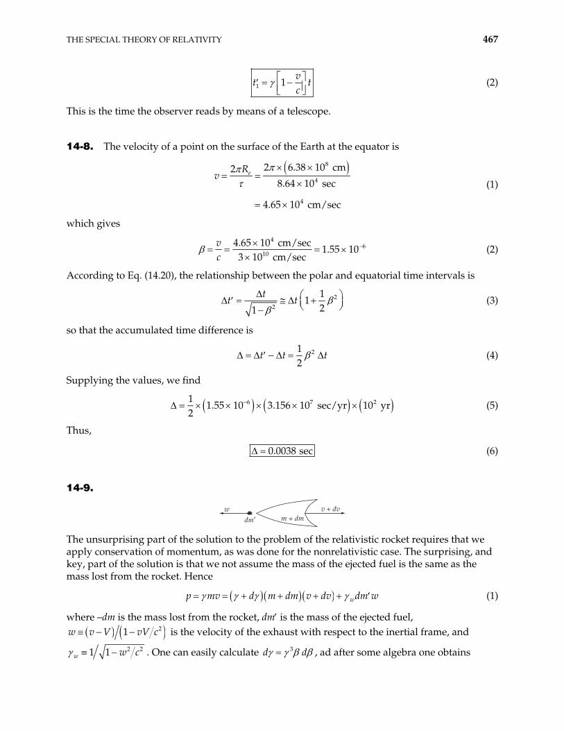
THE SPECIAL THEORY OF RELATIVITY 467
1 1v
tc
t (2)
This is the time the observer reads by means of a telescope.
14-8. The velocity of a point on the surface of the Earth at the equator is
8
4
4
2 6.38 10 cm28.64 10 sec
4.65 10 cm/sec
eRv
(1)
which gives
4
610
4.65 10 cm/sec1.55 10
3 10 cm/secvc
(2)
According to Eq. (14.20), the relationship between the polar and equatorial time intervals is
2
2
11
21
tt t (3)
so that the accumulated time difference is
212
t t t (4)
Supplying the values, we find
6 711.55 10 3.156 10 sec/yr 10 yr
22 (5)
Thus,
0.0038 sec (6)
14-9.
wdm! m + dm
v + dv
The unsurprising part of the solution to the problem of the relativistic rocket requires that we apply conservation of momentum, as was done for the nonrelativistic case. The surprising, and key, part of the solution is that we not assume the mass of the ejected fuel is the same as the mass lost from the rocket. Hence
wp mv d m dm v dv dm w (1)
where –dm is the mass lost from the rocket, dm is the mass of the ejected fuel, 21w v V vV c is the velocity of the exhaust with respect to the inertial frame, and
2 21 1w w c . One can easily calculate 3d d , ad after some algebra one obtains
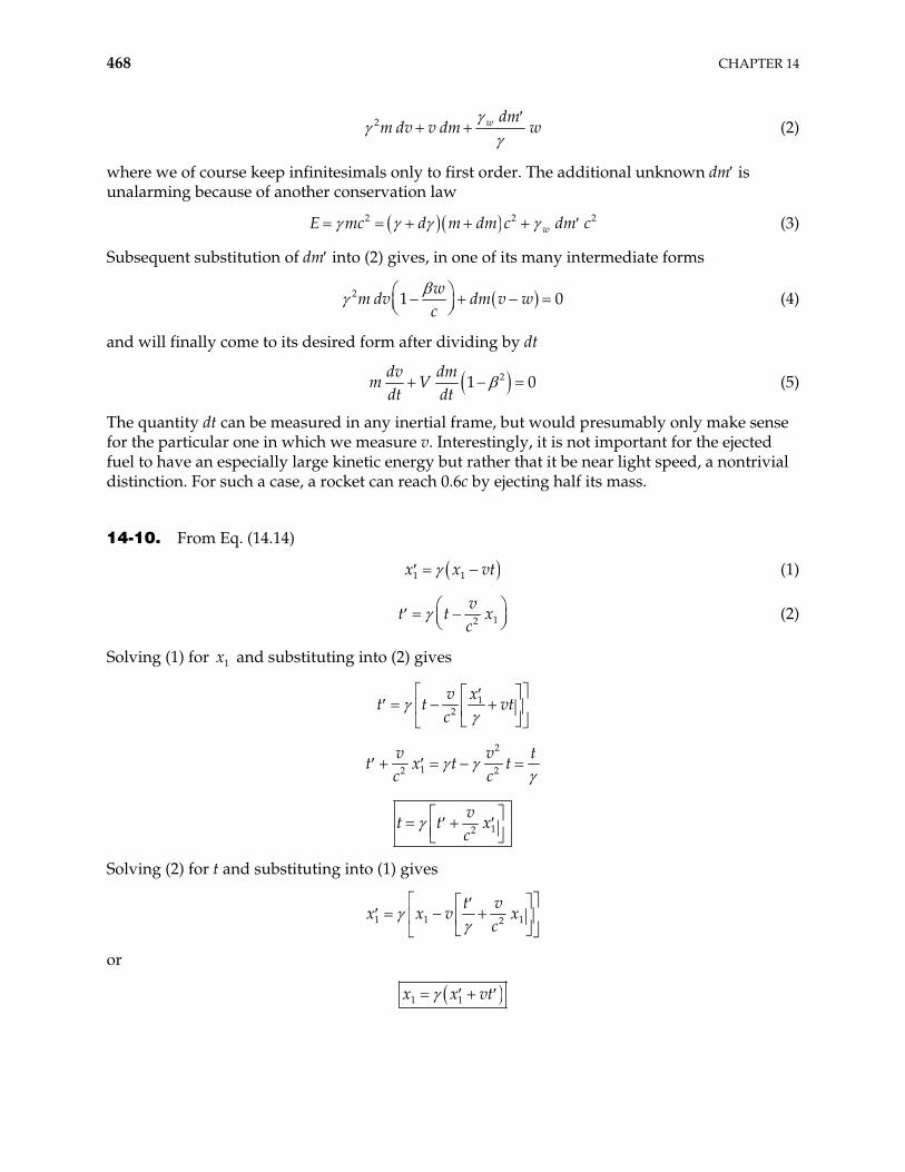
468 CHAPTER 14
2 w dmm dv v dm w (2)
where we of course keep infinitesimals only to first order. The additional unknown dm is unalarming because of another conservation law
2 2wc d m dm c dm c2E m (3)
Subsequent substitution of dm into (2) gives, in one of its many intermediate forms
2 1w
m dv dm v wc
0 (4)
and will finally come to its desired form after dividing by dt
21dv dm
m Vdt dt
0 (5)
The quantity dt can be measured in any inertial frame, but would presumably only make sense for the particular one in which we measure v. Interestingly, it is not important for the ejected fuel to have an especially large kinetic energy but rather that it be near light speed, a nontrivial distinction. For such a case, a rocket can reach 0.6c by ejecting half its mass.
14-10. From Eq. (14.14)
1 1x x vt (1)
12
vt t x
c (2)
Solving (1) for and substituting into (2) gives 1x
12
xvt t vt
c
2
12 2
v vt x t t
c ct
12
vt t x
c
Solving (2) for t and substituting into (1) gives
1 1 12
t vx x v x
c
or
1 1x x vt
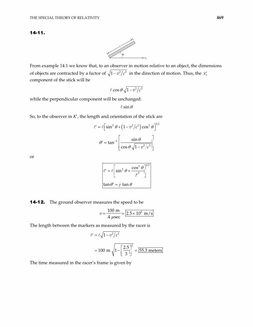
THE SPECIAL THEORY OF RELATIVITY 469
14-11.
"
x1 From example 14.1 we know that, to an observer in motion relative to an object, the dimensions
of objects are contracted by a factor of 2 21 v c in the direction of motion. Thus, the 1x component of the stick will be
2 2cos 1 v c
while the perpendicular component will be unchanged:
sin
So, to the observer in K , the length and orientation of the stick are
1 22 2 2 2sin 1 cosv c
1
2 2
sintan
cos 1 v c
or
1 222
2
cossin
tan tan
14-12. The ground observer measures the speed to be
8100 m2.5 10 m/s
.4 secv
The length between the markers as measured by the racer is
2 2
2
1
2.5100 m 1 55.3 meters
3
v c
The time measured in the racer’s frame is given by
470 CHAPTER 14
12
8
2
2
2.5 10 m/s 100 m.4 sec
1 2.5 3
.22 sec
vt t x
c
c
The speed observed by the racer is
82.5 10 m/svt t
14-13.
1 22
1.5 s
1 0.999 22.4
t t
t
Therefore 34 st .
14-14.
K K!
receiver
v
source In K, the energy and momentum of each photon emitted are
00 and
hE h p
c
Using Eq. (14.92) to transform to K :
01 1
0 0
;h
E h E vp pc
vh h
c
THE SPECIAL THEORY OF RELATIVITY 471
So
0
0 02
1
1 111
vc
which agrees with Eq. (14.31).
14-15. From Eq. (14.33)
011
Since c
011
or
011
With 0 656.3 nm and 4
8
4 103 10
, = 656.4 nm.
S o the shift is 0.1 nm toward the red (longer wavelength).
14-16.
"
"!
Earth
star
v
K!
K
Consider a photon sent from the star to the Earth. From Eq. (14.92)
1E E vp
also
1E E vp
472 CHAPTER 14
Now
00 1 1, , cos , cos
hhE h p p
c cE h
Substituting yields
0 1 cos
and
0 1 cos
Thus
21 cos 1 cos
1 2 2cos cos cos cos 1
cos cos cos cos
Solving for cos yields
cos
cos1 cos
where
angle in earth’s frame
angle in star’s frame
v c
14-17. From Eq. (14.33)
011
Since
c ,
011
We have 01.5 . This gives 5
13
or
81.2 10 m/secv
THE SPECIAL THEORY OF RELATIVITY 473
14-18.
"
observer
source
light
v
K!
K
Proceeding as in example 14.11, we treat the light as a photon of energy h .
In 00: ,
hh p
cK E
In 1: h E pK E
For the source approaching the observer at an early time we have
01
hp
c
Thus
0 0 011
vc
For the source receding from the observer (at a much later time) we have
01
hp
c
and
011
So
0
0
1source approaching observer
1
1source receding from observer
1
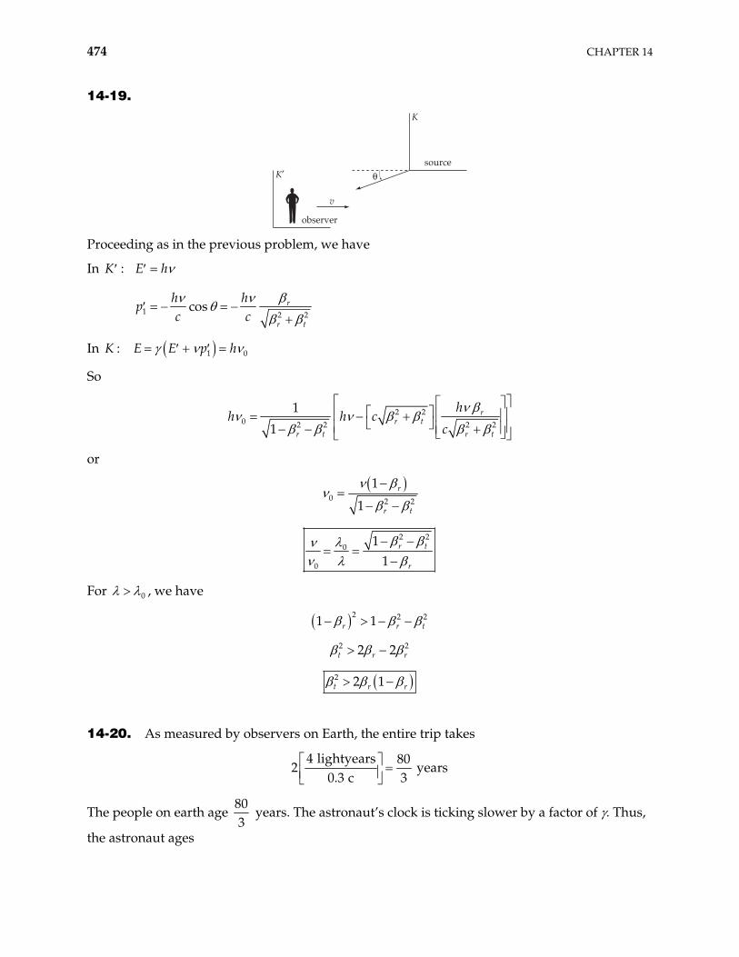
474 CHAPTER 14
14-19.
"
observer
source
v
K
K!
Proceeding as in the previous problem, we have
In
1 2 2
:
cos r
r t
K E h
h hp
c c
In 1 0:K E E p h
So
2 20 2 2 2 2
1
1r
r t
r t r t
hc
ch h
or
0 2 2
1
1r
r t
2 2
0
0
11
r t
r
For 0 , we have
2 2 21 1r r t
2 22 2t r r
2 2 1t r r
14-20. As measured by observers on Earth, the entire trip takes
4 lightyears 80
2 y0.3 c 3
ears
The people on earth age 803
years. The astronaut’s clock is ticking slower by a factor of . Thus,
the astronaut ages
THE SPECIAL THEORY OF RELATIVITY 475
280 801 0.3 0.95 years
3 3
So
Those on Earth age 26.7 years.The astronaut ages 25.4 years.
14-21. 00 3 22 2 2
0 3 22 2
1 22
1 1 1
1 1
mdF m
dt
m
v vv
v v
(1)
If we take (this does not mean v v1 1vv e 2 3 0 ), we have
1 1
101
1 0 13 2 3 22 2 21 1 1
v vv mv c c v m v1F m (2)
02 221
tm
2F v m v (3)
03 321
tm
3F v m v (4)
14-22. The total energy output of the sun is
3 21.4 10 W m 4dE
Rdt
2 (1)
where is the mean radius of the Earth’s orbit around the sun. Therefore, 111.50 10 mR
263.96 10 WdEdt
(2)
The corresponding rate of mass decrease is
92
14.4 10 kg s
dm dEdt c dt
1 (3)
The mass of the sun is approximately 1. , so this rate of mass decrease can continue for a time
3099 10 kg
476 CHAPTER 14
30
139 1
1.99 10 yr1.4 10 yr
4.4 10 kg sT (4)
Actually, the lifetime of the sun is limited by other factors and the sun is expected to expire about years from now. 94.5 10
14-23. From Eq. (14.67)
2 2 2 20
2 20 0
20
2 2 2 2
2
2
p c E E
E T E
E T T
p c T mc T
14-24. The minimum energy will occur when the four particles are all at rest in the center of the mass system after the collision.
Conservation of energy gives (in the CM system)
22 4p pE m c
or
2,CM 02 2p pE m c E
which implies = 2 or 3 2
To find the energy required in the lab system (one proton at rest initially), we transform back to the lab
1E E vp (1)
The velocity of K (CM) with respect to K(lab) is just the velocity of the proton in the K system. So u = v.
Then
2 21 CMv p v mu mv mc 2vp
Since = 2, 3 2 ,
1 032
vp E
Substituting into (1)
THE SPECIAL THEORY OF RELATIVITY 477
lab 0 0 0 03 7
2 22 2
E E E E 7E
2 2 The minimum proton energy in the lab system
7 , of which 6 is kinetic energy.p pm cis m c
14-25. Let B z 0B
x yv vv i j
Then
0
0 0
00 0x y
y x
q q v vB
q v B v B
i j kv B
i j
d dq m
dt dtF v B p v gives
0y x
qBdv v
dt mv i j
Define 0q B m
Thus
and x y y xv v v v
or
2x y xv v v
and
2y x yv v v
t
t
So
cos sin
cos sin
x
y
v A t B
v C t D
Take 0xv v , 0yv 0 . Then A = v, C = 0. Then 0 0x y 0v v
0 0
0,
y xv v
B D v
v
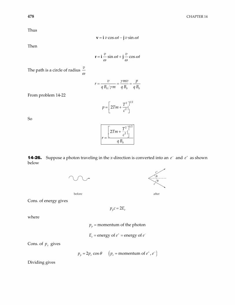
478 CHAPTER 14
Thus
cos sinv t v tv i j
Then
sin cosv v
t tr i j
The path is a circle of radius v
0 0 0
pv mvr
q B m q B q B
From problem 14-22
1 22
22T
p Tmc
So
1 22
2
0
2 TTm
cr
q B
14-26. Suppose a photon traveling in the x-direction is converted into an e and as shown below
e
before after
e+
e–
""
Cons. of energy gives
2p ep c E
where
momentum of the photon
energy of energy of
p
e
p
E e e
Cons. of gives xp
2 cos momentum of ,p e ep p p e e
Dividing gives
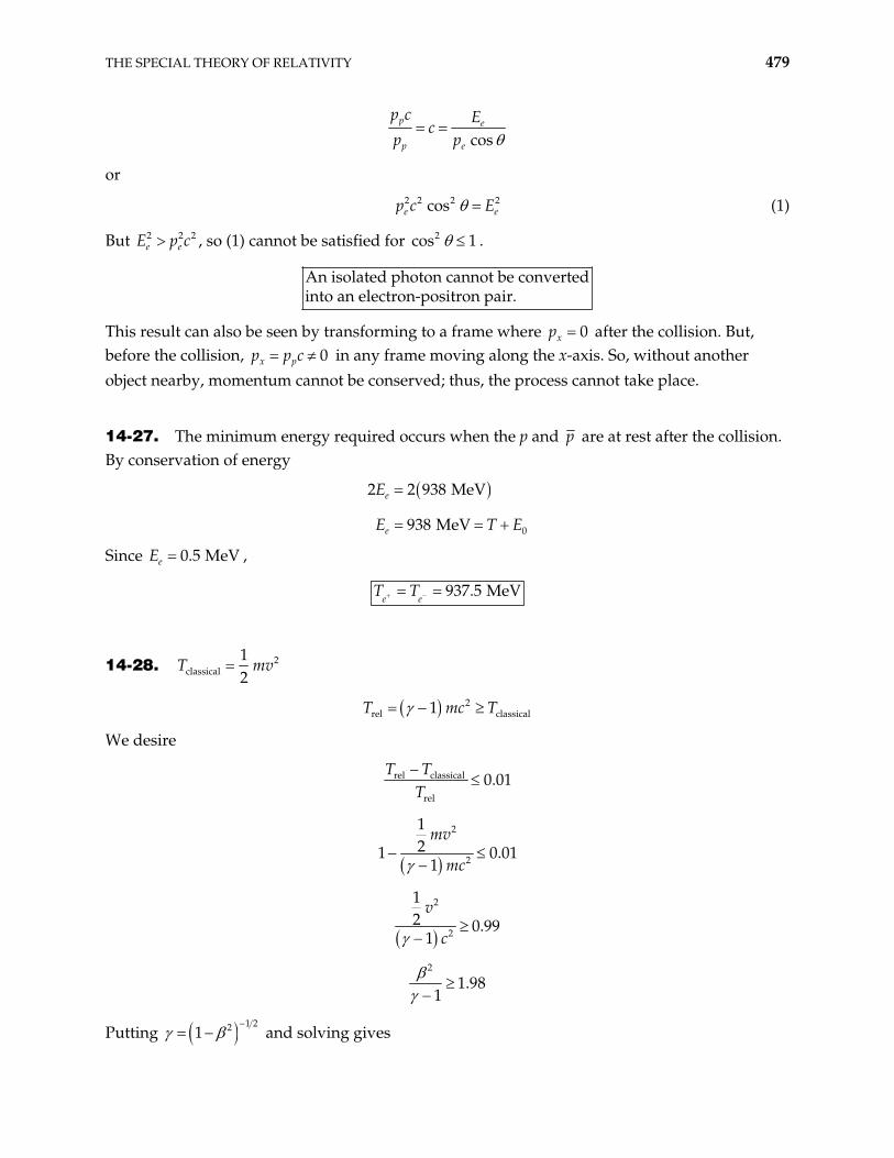
THE SPECIAL THEORY OF RELATIVITY 479
cos
p e
p e
p c Ec
p p
or
2 2 2 2cose ep c E (1)
But , so (1) cannot be satisfied for 2 2e eE p c2 2cos 1 .
An isolated photon cannot be converted
to an electron-positron pair.in
This result can also be seen by transforming to a frame where 0xp after the collision. But, before the collision, 0x pp p c in any frame moving along the x-axis. So, without another object nearby, momentum cannot be conserved; thus, the process cannot take place.
14-27. The minimum energy required occurs when the p and p are at rest after the collision. By conservation of energy
0
2 2 938 MeV
938 MeV
e
e
E
E T E
Since E , 0.5 MeVe
937.5 MeVe e
T T
14-28. 2classical
12
T mv
2rel classical1T mc T
We desire
rel classical
rel
0.01T T
T
2
2
121 0
1
mv
mc.01
2
2
12 0.99
1
v
c
2
1.981
Putting 1 221 and solving gives
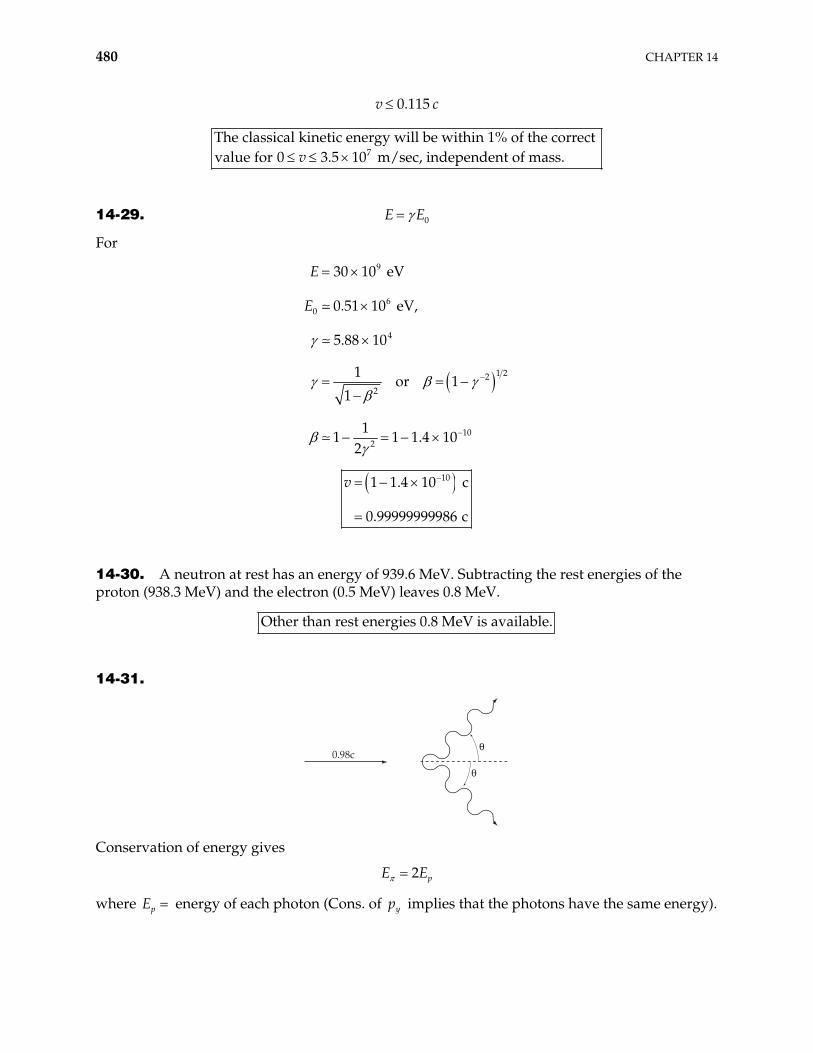
480 CHAPTER 14
0.115v c
7The classical kinetic energy will be within 1% of the correct
for 0 3.5 10 m/sec, independent of mass.vvalue
14-29. 0E E
For
9
60
4
1 22
2
102
30 10 eV
0.51 10 eV,
5.88 10
1or 1
1
11 1 1.4 10
2
E
E
101 1.4 10 c
0.99999999986 c
v
14-30. A neutron at rest has an energy of 939.6 MeV. Subtracting the rest energies of the proton (938.3 MeV) and the electron (0.5 MeV) leaves 0.8 MeV.
Ot her than rest energies 0.8 MeV is available.
14-31.
0.98c"
"
Conservation of energy gives
2 pE E
where E energy of each photon (Cons. of p yp implies that the photons have the same energy).
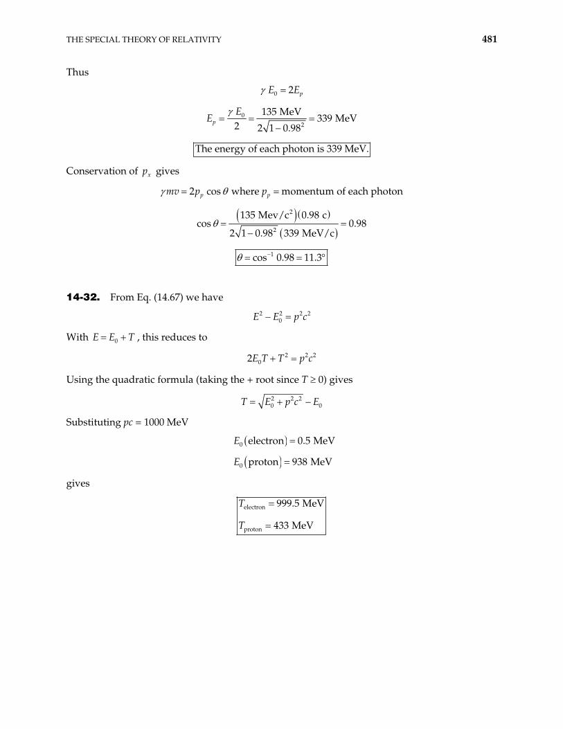
THE SPECIAL THEORY OF RELATIVITY 481
Thus
0 2 pE E
02
135 MeV339 MeV
2 2 1 0.98p
EE
Th e energy of each photon is 339 MeV.
Conservation of gives xp
mv 2 cos where momentum of each photonp pp p
2
2
135 Mev/c 0.98 cs 0.98
2 1 0.98 339 MeV/cco
1cos 0.98 11.3
14-32. From Eq. (14.67) we have
2 2 20E E p c2
2
With , this reduces to 0E E T
2 202E T T p c
Using the quadratic formula (taking the + root since T 0) gives
2 2 20 0T E p c E
Substituting pc = 1000 MeV
0 electron 0.5 MeVE
0 proton 938 MeVE
gives
electron
proton
999.5 MeV
433 MeV
T
T
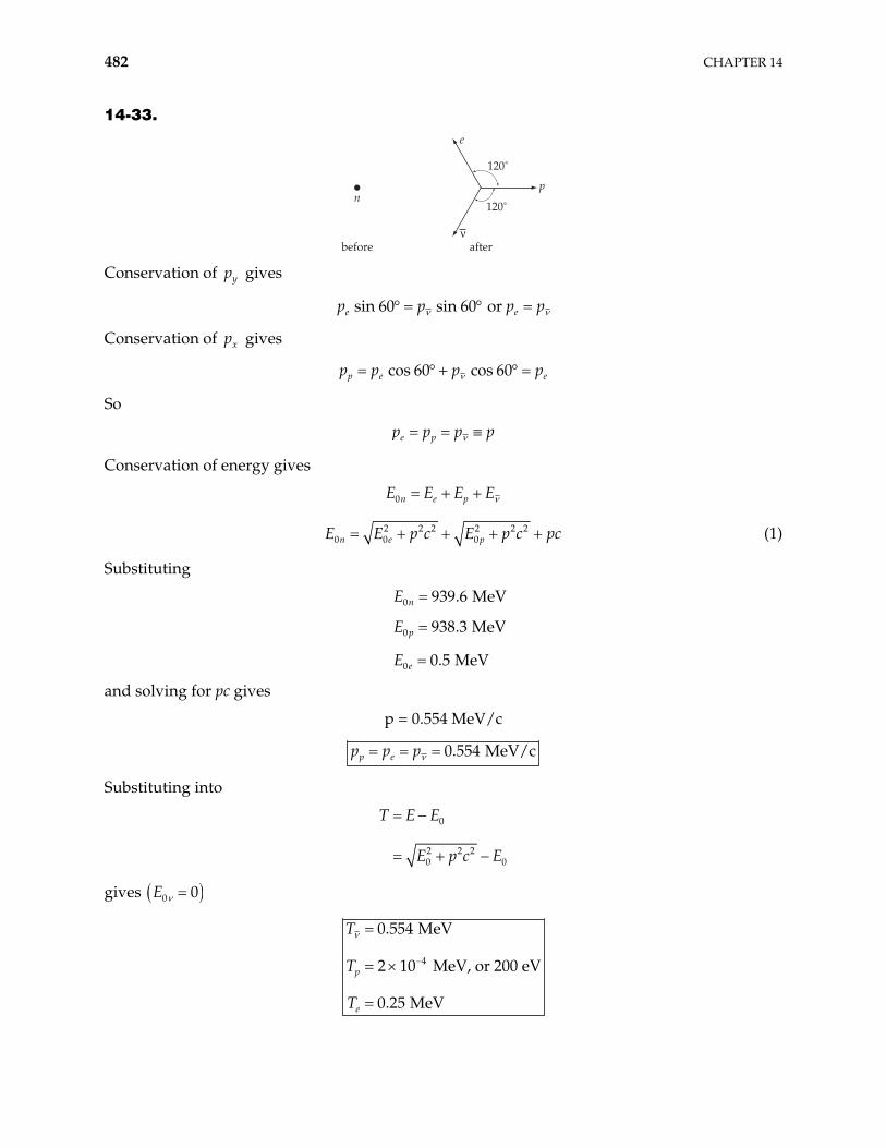
482 CHAPTER 14
14-33.
120˚
120˚
afterbefore
p
e
n
#
Conservation of yp gives
sin 60 sin 60 or e ep p p p
Conservation of gives xp
cos 60 cos 60p e ep p p p
So
e pp p p p
Conservation of energy gives
0n e pE E E E
2 2 2 2 2 20 0 0n e pE E p c E p c pc (1)
Substituting
0 939.6 MeVnE
0 938.3 MeVpE
0 0.5 MeVeE
and solving for pc gives
p = 0.554 MeV/c
0.554 MeV/cp ep p p
Substituting into
0
2 2 20 0
T E E
E p c E
gives 0 0E
4
0.554 MeV
2 10 MeV, or 200 eV
0.25 MeV
p
e
T
T
T
THE SPECIAL THEORY OF RELATIVITY 483
14-34. 2 2 2 2 2 21 2s c t x x x3
Using the Lorentz transformation this becomes
2 22 2 1
2 2 2122 21 1
2 32 2 2 2
2 2 22 2 2 211 2 2
2 22 32 2
2 2 2 2 21 2 3
2 21 1
1
v xc t x vt x v t x vtcs x
v c v c
v x vx c t t
c cx x
v c
c t x x x
2x
So
2 2s s
14-35. Let the frame of Saturn be the unprimed frame, and let the frame of the first spacecraft be the primed frame. From Eq. (14.17a) (switch primed and unprimed variables and change the sign of v)
11
121
u vu u v
c
Substituting v = 0.9 c
1 0.2u c
gives
1 0.93u c
14-36. Since
1 2 3 and , , ,d dX
X x x x id d
F m ct
we have
21 1
1 2
2232
2 32 2
2
4 2
dx d xdF m m
d d d
d xd xF m F m
d d
d ictd dF m icm
d d dt
484 CHAPTER 14
Thus
2 21
1 12 2
2 21
1 42 2
2 22 2
2 22 2
14 2 2
221
2 2
4 1
;
d x dF m m x vt
d d
d x d tm mv F i
d d
d x d xF m m F F F
d d
vxdF icm t
d c
d xd ticm i m
d d
F i F
3 3
F
Th us the required transformation equations are shown.
14-37. From the Lagrangian
2 2 11 1
2L mc kx2 (1)
we compute
L
kxx
(2)
21
L Lmc
v v (3)
Then, from (2) and (3), the Lagrange equation of motion is
2
01
d mckx
dt (4)
from which
3 220
1
mckx (5)
Using the relation
dv dv dx dv
cdt dx dt dx
v (6)
we can rewrite (4) as
THE SPECIAL THEORY OF RELATIVITY 485
2
3 220
1
mc dkx
dx (7)
This is easily integrated to give
2
2
2
121
mckx E (8)
where E is the constant of integration.
The value of E is evaluated for some particular point in phase space, the easiest being x = a; = 0:
2 12
E mc ka2 (9)
From (8) and (9),
2
2 2
2
1 12 21
mckx mc ka2 (10)
Eliminating 2 from (10), we have
2 42
22 2 2
2 2 2
2 22
2 2 2
112
4
2
m c
mc k a x
kmc a xk a x
kmc a x
(11)
and, therefore,
2 2 2 2 2
2 2 2
412
k a x mc k a xdxc dt mc k a x
(12)
The period will then be four times the integral of dt = dt(x) from x = 0 to x = a:
2 22
2 2 2 202
124
14
ak
a xm mc dxk k
a x a xmc
(13)
Since x varies between 0 and a, the variable x a takes on values in the interval 0 to 1, and therefore, we can define
sinxa
(14)
from which
486 CHAPTER 14
2 2
cosa x
a (15)
and
2 2dx a x d (16)
We also define the dimensionless parameter,
22a k
mc (17)
Using (14) – (17), (13) transforms into
2 22
2 20
1 2 cos2
1 cos
ad
c (18)
Since 2 2 1ka mc for the weakly relativistic case, we can expand the integrand of (18) in a series of powers of :
2 2 22 2 2
1 22 2
2 2
2 2
1 2 cos1 2 cos 1 cos
21 cos
11 2 cos
2
31 cos
2 (19)
Substitution of (19) into (18) yields
22 2
0
2
0
2 31 cos
2
3 1sin 2
2 2
ad
c
a ac c
(20)
Evaluating (20) and substituting the expression for from (17), we obtain
2
2
32
8m ak c
km
(21)
or,
2
0 2
31
16kamc
(22)
THE SPECIAL THEORY OF RELATIVITY 487
14-38.
(for constant)
dp dF mu
dt dt
dm u m
dt
2 21
d um
dt u c
1 2 1 22 2 2 22
2 2
1 1
1
uu c u u cducmdtu c
3 22 21
dum u c
dt
Thus
3 22 21
duF m u c
dt
14-39. The kinetic energy is
2 2 2 4 20 0T p c m c m c (1)
For a momentum of 100 MeV/c,
24proton 10 931 931 936 931 5 MeVT (2)
24electron 10 0.51 0.51 100 0.5 99.5 MeVT (3)
In order to obtain and , we use the relation
2
2 2 00 21
m cE mc m c (4)
so that
20
Em c
(5)
and
2
11 (6)
electron100
2000.51
(7)
488 CHAPTER 14
2
electron1
1 0.99200
9988 (8)
This is a relativistic velocity.
proton936
1.0054931
(9)
2
proton1
11.0053
0.1 (10)
This is a nonrelativistic velocity.
14-40. If we write the velocity components of the center-of-mass system as jv , the transformation of , jp into the center-of-mass system becomes
, , 2j
j j
v Ep p
c (1)
where 2
2
1
1 jvc
. Since in the center-of-mass system, , 0jp must be satisfied, we have
, , 2 0jj j
v Ep p
c (2)
or,
, j
jp cv
c E (3)
14-41. We want to compute
2
1 012
0 0 0
E m cTT E m c
(1)
where T and E represent the kinetic and total energy in the laboratory system, respectively, the subscripts 0 and 1 indicate the initial and final states, and is the rest mass of the incident particle.
0m
The expression for in terms of 0E 1 is
20 0E m c 1 (2)
1E can be related to (total energy of particle 1 in the center of momentum reference frame after the collision) through the Lorentz transformation [cf. Eq. (14.92)] (remembering that for the inverse transformation we switch the primed and unprimed variables and change the sign of v):
1E
THE SPECIAL THEORY OF RELATIVITY 489
1 1 1 1 1 cosE E c p
1
(3)
where 1 0 1p m c and E m 21 0c 1 :
2 2 21 0 1 11 cosE m c (4)
Then, from (1), (2), and (4),
2 2 2
1 1 11
0 1
cos 11
TT
(5)
For the case of collision between two particles of equal mass, we have, from Eq. (14.127),
2 11
12
(6)
and, consequently,
2 2 2 11 1 1
11
2 (7)
Thus, with the help of (6) and (7), (5) becomes
1 11
0 1
1 1 co2 1
1 cos2
TT
s
(8)
We must now relate the scattering angle in the center of momentum system to the angle in the lab system.
Squaring Eq. (14.128), which is valid only for 1m m2 , we obtain an equation quadratic in cos . Solving for cos in terms of tan2 , we obtain
21
21
1tan 1
2cos 11 tan
2
(9)
One of the roots given in (9) corresponds to = , i.e., the incident particle reverses its path and is projected back along the incident direction. Substitution of the other root into (8) gives
2
12
210 1
2 cos11 2 cos 1 sin1 tan
2
TT 2 (10)
An elementary manipulation with the denominator of (10), namely,
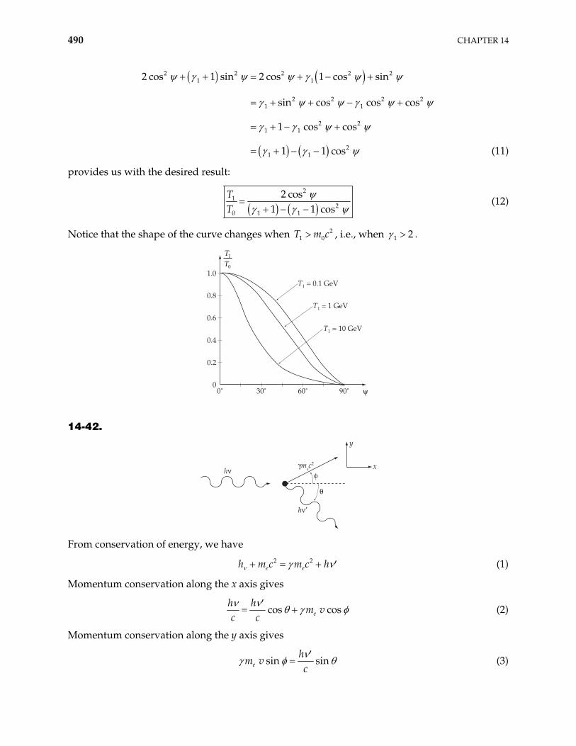
490 CHAPTER 14
2 2 2 2 21 1
2 2 2 21 1
2 21 1
21 1
2 cos 1 sin 2 cos 1 cos sin
sin cos cos cos
1 cos cos
1 1 cos (11)
provides us with the desired result:
2
12
0 1 1
2 cos1 1 cos
TT
(12)
Notice that the shape of the curve changes when T m , i.e., when 21 0c 1 2 .
0.2
00˚ 30˚ 60˚ 90˚
0.4
0.6
0.8
1.0
TT
1
0
T1 = 0.1 GeV
T1 = 1 GeV
T1 = 10 GeV
$
14-42.
%
"
h#
h#!
&mec2
y
x
From conservation of energy, we have
2 2e eh m c m c h (1)
Momentum conservation along the x axis gives
cos coseh h
m vc c
(2)
Momentum conservation along the y axis gives
sin sineh
m vc
(3)
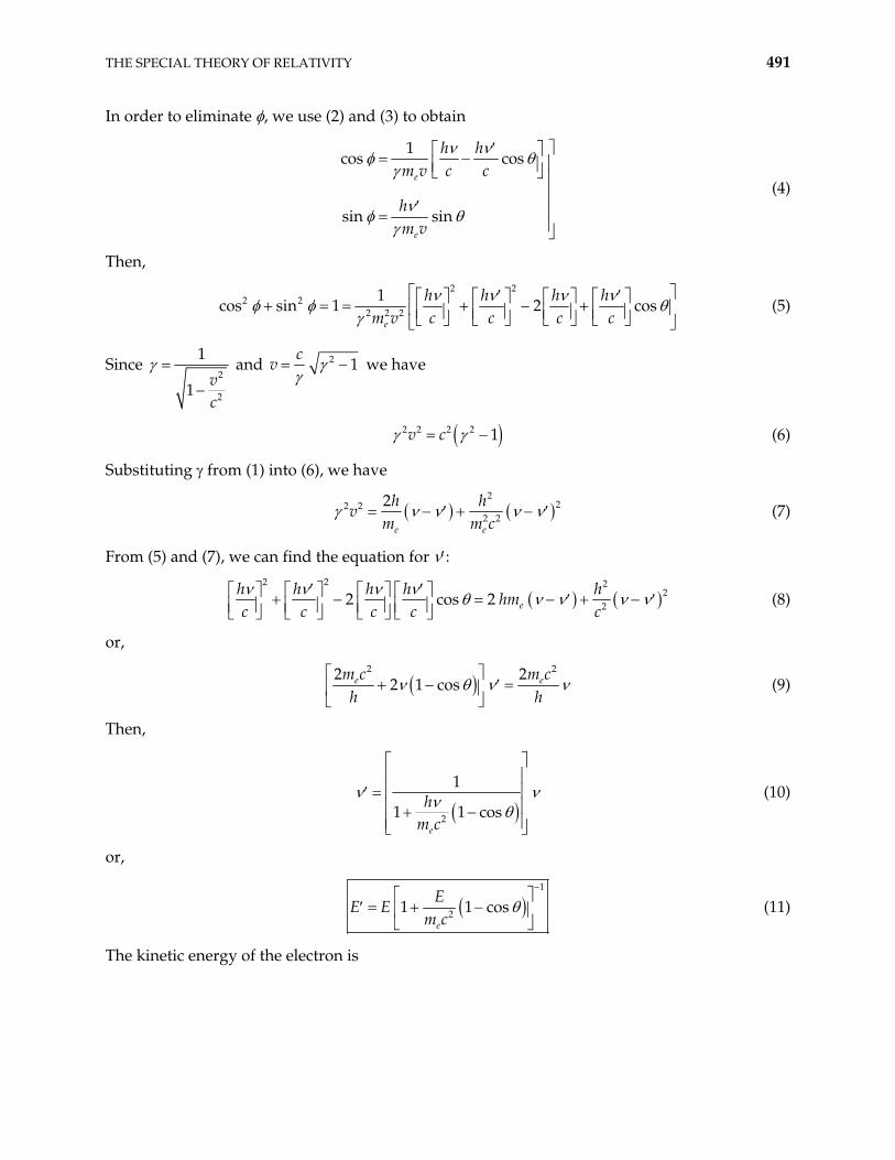
THE SPECIAL THEORY OF RELATIVITY 491
In order to eliminate , we use (2) and (3) to obtain
1cos cos
sin sin
e
e
h hm v c c
hm v
(4)
Then,
2 2
2 22 2 2
1s sin 1 2 cos
e
h h h hm v c c c c
co (5)
Since 2
2
1
1 vc
and 2 1c
v we have
2 2 2 2 1v c (6)
Substituting from (1) into (6), we have
2
22 22 2
2
e e
h hv
m m c (7)
From (5) and (7), we can find the equation for :
2 2 2
222 cos 2 e
h h h h hhm
c c c c c (8)
or,
2 22
2 1 cosem c m ch h
2 e (9)
Then,
2
1
1 1 cose
hm c
(10)
or,
1
21 1 cose
EE E
m c (11)
The kinetic energy of the electron is
492 CHAPTER 14
2 2
2
11
1 1 cose e
e
c m c h h E Em c
T m
2
2
2
1 cos
1 1 cose
e
ET Em c
m c
(12)