Solutions Chapter 5

Presented by Suong Jian & Liu Yan, MGMT Panel , Guangdong University of Finance.

- 134 -

Chapter 6 DEMAND ESTIMATION QUESTIONS & ANSWERS Q6.1 A linear approximation to the market demand curve for Chevy Trail Blazers assumes

a constant marginal effect of changes in price on the quantity demanded. Is this assumption valid at extraordinarily high prices, like $75,000, and at giveaway low prices, like $7,500?

Q6.1 ANSWER

No. Linear demand curves assume a constant marginal effect of changes in price, prices of other goods, income, advertising and other factors. It is vital to remember that this assumption is only valid within the range of observed data. When estimating the market demand curve, it is essential that analysis of the estimated model be confined to the range of data used to derive the model itself. For example, General Motors has very good information about the relationship between price and the quantity demanded of Chevrolet Trail Blazer SUVs, but only within the neighborhood of current prices. When GM offers a $2,500 rebate on Trail Blazers, it is able to gain sufficient information to derive a linear approximation to the underlying market demand curve. Nobody knows how many Trail Blazers would be purchased at an extraordinarily high price, like $75,000, nor at a giveaway low price, like $7,500. Those prices are irrelevant to the company=s present production, pricing and promotion decisions. What a linear approximation to the firm=s market demand curve can do is provide valuable information around the present suggested retail price near $35,000-$40,000.

Q6.2 Explain how shifting demand and supply curves make market demand estimation

difficult. Q6.2 ANSWER

The identification problem relates to the difficulty encountered in properly isolating independent variables (X factors) that influence a given dependent variable (Y factor). To accurately model the demand function for a given product, the effects of all relevant independent variables must be incorporated. Moreover, these independent influences must be reflected using an appropriate linear or log-linear model. The process of accurately modeling the link between dependent Y variables and

Demand Estimation


- 135 -

independent X variables is made difficult by the dynamic nature of demand relations. The identification problem is especially troublesome in demand estimation because many factors that influence demand also influence supply. When demand and supply relations are so interrelated as to make accurate empirical estimation futile, it becomes impossible to identify each individual function.

Q6.3 ARapid innovation in the development, assembly, and delivery of personal computers

has led to a sharply downward sloping market demand curve for Dell, Inc.@ Discuss this statement.

Q6.3 ANSWER

This statement is false, and reflects a basic misconception concerning the differences between shifts in demand and movements along a demand curve. A market demand curve shows the relation between the price charged and the quantity demanded, holding constant the effects of all other variables in the demand function. To plot a demand curve, it is necessary to obtain data on the price/quantity relation, while keeping fixed all other factors in the demand function. Rapid innovation in the development, assembly, and delivery of personal computers has led to an increase in market demand for personal computers. This is reflected in a rightward shift in the market demand curve, not in a downward movement along the market demand cure, holding product quality and the level of innovation constant.

Q6.4 ADemand for higher education is highest among the wealthy. This has led to an

upward sloping demand curve for college education. The higher the tuition charged, the greater is demand.@ Discuss this statement.

Q6.4 ANSWER

This statement is false, and reflects a basic misconception concerning the differences between shifts in demand and movements along a demand curve. A market demand curve shows the relation between the price charged and the quantity demanded, holding constant the effects of all other variables in the demand function. To plot a demand curve, it is necessary to obtain data on the price/quantity relation, while keeping fixed all other factors in the demand function. As income rises, it is reasonable to expect an increase in market demand for higher education. This is reflected in a rightward shift in the market demand curve, not in a downward movement along the market demand curve, holding product quality and the level of income constant. Now, in terms of college education, a caveat may be in order. To the extent that consumers are poorly informed about the quality of various colleges

Chapter 6


- 136 -

and universities, some consumers may use the amount of tuition charged as a proxy for product quality. For such uninformed consumers, the quantity demanded might in fact rise with tuition when they assume high tuition rates signal high academic quality.

Q6.5 How do linear and log-linear models differ in terms of their assumptions about the

nature of demand elasticities? Q6.5 ANSWER

The elasticity of demand is defined as the percentage change in demand following a 1 per cent change in a given demand-determining variable. In the linear model approach, the effect on demand of a one-unit change in any independent variable is assumed to be constant. This leads to changing elasticities of demand at different points along the linear demand curve. In the log-linear model approach, the effect of a one-unit change in any independent variable will tend to vary, but the elasticities of demand are assumed to be constant. Therefore, linear models involve an underlying assumption of changing elasticities; log-linear models assume constant elasticities.

Q6.6 Describe some of the limitations of market experiments. Q6.6 ANSWER

Market experiments have several serious shortcomings. They are expensive and usually undertaken on a scale too small to allow high levels of confidence in the results. Market experiments are seldom run for sufficiently long periods to indicate the long-run effects of various price, advertising, or packaging strategies. Difficulties associated with uncontrolled parts of market experiments also hinder their use. Changing economic conditions during the experiment can invalidate the results, especially if the experiment includes several separate markets. A local strike, layoffs by a major employer, or a severe snowstorm can ruin a market experiment. Likewise, a change in a competing product's promotion, price, or packaging can distort the results. There is also the danger that customers lost during the experiment as a result of price manipulations may not be regained when the experiment ends.

In some controlled laboratory experiments consumers are given funds and asked to shop in a simulated store. By varying prices, product packaging, displays, and other factors, the experimenter can learn a great deal about consumer behavior. Laboratory experiments provide information similar to that of field experiments, but have the advantages of lower cost and greater control of extraneous factors. However, subjects invariably know that they are part of an experiment, and this can

Demand Estimation


- 137 -

distort shopping habits. They may, for example, exhibit considerably more price consciousness than is typical in their everyday shopping. Moreover, the high cost of such experiments necessarily limits the sample size, which can make inference from the sample to the general population tenuous.

Q6.7 If a regression model estimate of total profit is $50,000 with a standard error of the

estimate of $25,000, what is the chance of an actual loss? Q6.7 ANSWER

The standard error of the estimate can be used to determine a range within which the dependent Y variable can be predicted with varying degrees of statistical confidence based on the regression coefficients and values for the X variables. Because the best estimate of the tth value for the dependent variable is ^Y t, as predicted by the regression equation, the standard error of the estimate can be used to determine just how accurate a prediction ^Y t is likely to be. If the ut error terms are normally distributed about the regression equation, as would be true when large samples of more than 120 or so observations are analyzed, there is a 95 per cent probability that observations of the dependent variable will lie within the range ^Y t ∀ (1.96 Η SEE), or within roughly two standard errors of the estimate. Because the 5 per cent rejection region is evenly split between each tail of the distribution, there is a 2.5 per cent chance of encountering an observation that is two standard deviations below the fitted value. In this question, there is a 2.5 per cent chance that actual profits will fall below $0, or more than two standard deviations below the expected value of $50,000.

Q6.8 A simple regression TR = a + bQ is not able to explain 19 per cent of the variation

in total revenue. What is the coefficient of correlation between TR and Q? Q6.8 ANSWER

In a simple regression model with only one independent variable the correlation coefficient, r, measures goodness of fit. The correlation coefficient falls in the range between 1 and -1. If r = 1, there is a perfect direct linear relation between the dependent Y variable and the independent X variable. If r = -1, there is a perfect inverse linear relation between Y and X. In both instances, actual values for Yt all fall exactly on the regression line. The regression equation explains all of the underlying variation in the dependent Y variable in terms of variation in the independent X variable. If r = 0, zero correlation exists between the dependent and independent variables; they are autonomous. When r = 0, there is no relation at all between actual

Chapter 6


- 138 -

Yt observations and fitted ^Y t values. The squared value of the coefficient of correlation, called the coefficient of

determination or R2, shows how well a regression model explains changes in the value of the dependent Y variable. R2 is defined as the proportion of the total variation in the dependent variable that is explained by the full set of independent variables. Thus, when a given regression model is unable to explain 19 per cent of the variation in the dependent Y variable (total revenue), explained variation equals 81 per cent . In such an instance, the square root of the coefficient of determination, equal to the correlation coefficient, equals 0.9 or 90 percent.

Q6.9 In a regression-based estimate of a demand function, the beta coefficient for

advertising equals 3.75 with a standard deviation of 1.25 units. What is the range within which there can be 99 per cent confidence that the actual parameter for advertising can be found?

Q6.9 ANSWER

The standard error of the estimate indicates the precision with which the regression model can be expected to predict the dependent Y variable. The standard deviation (or standard error) of each individual coefficient provides a similar measure of precision for the relation between the dependent Y variable and a given X variable. When the standard deviation of a given estimated coefficient is small, a strong relation is suggested between X and Y. When the standard deviation of a coefficient estimate is relatively large, the underlying relation between X and Y is typically weak. As a rough rule-of-thumb, assuming a typical regression model of four or five independent X variables plus an intercept term, a calculated t-statistic greater than two permits rejection of the hypothesis that there is no relation between the dependent Y variable and a given X variable at the α = 0.05 significance level (with 95 per cent confidence). A calculated t-statistic greater than three typically permits rejection of the hypothesis that there is no relation between the dependent Y variable and a given X variable at the α = 0.01 significance level (with 99 per cent confidence). Similarly, there is roughly a 95 per cent chance that the actual parameter lies in the range b ∀ (2 Η S.E.), and a 99 per cent chance that the actual parameter lies in the range b ∀ (3 Η S.E.). If the b-coefficient for advertising equals 3.75 with a standard deviation of 1.25 units, there can be 99 per cent confidence that the actual parameter for advertising lies in the range 3.75 ∀ (3 Η 1.25), or from 0 to 7.5 units.

Q6.10 Managers often study the profit margin-sales relation over the life cycle of individual

products, rather than the more direct profit-sales relation. In addition to the

Demand Estimation


- 139 -

economic reasons for doing so, are there statistical advantages as well? (Note: Profit margin equals profit divided by sales.)

Q6.10 ANSWER

Yes, managers study the profit margin-sales relation over the life cycle of individual products and for individual products at any one point in time to gauge relative profitability. High profit margins are attractive as they suggest unique product characteristics that are valued by customers. If profit margins deteriorate over time, this means that distinctive features valued by customers have been eroded by competition or changing consumption patterns. In addition to the economic advantages for analyzing profit margin-sales relations rather than profit-sales relations, there are important statistical advantages as well. Both sales and profit data embody a size element--big firms tend to report large sales and profit numbers. As a result, there is often a link between firm size and the size or variability of disturbance terms for any given profit-sales relation. A residual sequence plot is often used to indicate whether or not the variance of the residual term is constant over the entire sample. Common corrective action for this heteroskedasticity problem is to transform the regression variables into logarithmic or ratio form prior to estimation, or rely on more sophisticated weighted least squares regression methods.

SELF-TEST PROBLEMS & SOLUTIONS STP6.1 Linear Demand Curve Estimation. Women=s NCAA basketball has enjoyed

growing popularity across the country, and benefitted greatly from sophisticated sports marketing. Savvy institutions use time-tested means of promotion, especially when match-ups against traditional rivals pique fan interest. As a case in point, fan interest is high whenever the Arizona State Sun Devils visit Tucson, Arizona, to play the Arizona Wildcats. To ensure a big fan turnout for this traditional rival, suppose the University of Arizona offered one-half off the $16 regular price of reserved seats, and sales jumped from 1,750 to 2,750 tickets.

A. Calculate ticket revenues at each price level. Did the pricing promotion

increase or decrease ticket revenues?

B. Estimate the reserved seat demand curve, assuming that it is linear.

C. How should ticket prices be set to maximize total ticket revenue? Contrast this

Chapter 6


- 140 -

answer with your answer to part A. STP6.1 SOLUTION A. The total revenue function for the Arizona Wildcats is: TR = P Η Q

Then, total revenue at a price of $16 is: TR = P Η Q = $16 Η 1,750 = $28, 000

Total revenue at a price of $8 is: TR = P Η Q = $8 Η 2,750 = $22,000

The pricing promotion caused a decrease in ticket revenues. B. When a linear demand curve is written as: P = a + bQ

a is the intercept and b is the slope coefficient. From the data given previously, two points on this linear demand curve are identified. Given this information, it is possible to exactly identify the linear demand curve by solving the system of two equations with two unknowns, a and b:

16 = a + b(1,750) minus 8 = a + b(2,250) 8 = -1,000 b b = -0.008

Demand Estimation


- 141 -

By substitution, if b = -0.008, then: 16 = a + b(1,750) 16 = a - 0.008(1,750) 16 = a - 14 a = 30

Therefore, the reserved seat demand curve can be written: P = $30 - $0.008Q C. To find the revenue-maximizing output level, set MR = 0, and solve for Q. Because TR = P Η Q = ($30 - $0.008Q)Q = $30Q - $0.008Q2 MR = ΜTR/ΜQ MR = $30 - $0.016Q = 0 0.016Q = 30 Q = 1,875

At Q = 1,875, P = $30 - $0.008(1,875) = $15

Total revenue at a price of $15 is: TR = P Η Q

Chapter 6


- 142 -

= $15 Η 1,875 = $28,125

(Note: Μ2TR/ΜQ2 < 0. This is a ticket-revenue maximizing output level because total ticket revenue is decreasing for output beyond Q > 1,875.)

ST6.2 Regression Analysis. The use of regression analysis for demand estimation can be

further illustrated by expanding the Electronic Data Processing (EDP), Inc., example described in the chapter. Assume that the link between units sold and personal selling expenditures described in the chapter gives only a partial view of the impact of important independent variables. Potential influences of other important independent variables can be studied in a multiple regression analysis of EDP data on contract sales (Q), personal selling expenses (PSE), advertising expenditures (AD), and average contract price (P). Because of a stagnant national economy, industry-wide growth was halted during the year, and the usually positive effect of income growth on demand was missing. Thus, the trend in national income was not relevant during this period. For simplicity, assume that relevant factors influencing EDP's monthly sales are as follows:

Units Sold, Price, Advertising and Personal Selling Expenditures for

Electronic Data Processing, Inc. Month

Units Sold

Price

Advertising Expenditures

Personal Selling

Expenditures January

2,500

$3,800

$26,800

$43,000

February

2,250

3,700

23,500

39,000 March

1,750

3,600

17,400

35,000

April

1,500

3,500

15,300

34,000 May

1,000

3,200

10,400

26,000

June

2,500

3,200

18,400

41,000 July

2,750

3,200

28,200

40,000

August

1,750

3,000

17,400

33,000 September

1,250

2,900

12,300

26,000

October

3,000

2,700

29,800

45,000 November

2,000

2,700

20,300

32,000

Demand Estimation


- 143 -

Units Sold, Price, Advertising and Personal Selling Expenditures for

Electronic Data Processing, Inc. Month

Units Sold

Price

Advertising Expenditures

Personal Selling

Expenditures December

2,000

2,600

19,800

34,000

Average 2,020.83

$3,175.00

$19,966.67

$35,666.67

If a linear relation between unit sales, contract price, advertising, and personal

selling expenditures is hypothesized, the EDP regression equation takes the following form:

where Y is the number of contracts sold, P is the average contract price per month, AD is advertising expenditures, PSE is personal selling

expenses, and u is a random disturbance term--all measured on a monthly basis over the past year.

When this linear regression model is estimated over the EDP data, the following regression equation is estimated (t-statistics in parentheses):

where Pt is price, ADt is advertising, PSEt is selling expense, and t-statistics are indicated within parentheses. The standard

error of the estimate or SEE is 123.9 units, the coefficient of determination or R2 = 97.0%, the adjusted coefficient of determination is 2

R = 95.8%, and the relevant F statistic is 85.4.

A. What is the economic meaning of the b0 = -117.513 intercept term? How

would you interpret the value for each independent variable's coefficient estimate?

B. How is the standard error of the estimate (SEE) employed in demand

estimation?

C. Describe the meaning of the coefficient of determination, R2, and the adjusted coefficient of determination, 2.R

D. Use the EDP regression model to estimate fitted values for units sold and

t t t0 P AD PSE t tSales = = + + + + b b b b PSE uY P AD

t tt t = -117.513 - 0.296 + 0.036 + 0.066Units PSEP AD(-0.35) (-2.91) (2.56) (4.61)

Chapter 6


- 144 -

unexplained residuals for each month during the year. ST6.2 SOLUTION A. The intercept term b0 = -117.513 has no clear economic meaning. Caution must

always be exercised when interpreting points outside the range of observed data and this intercept, like most, lies far from typical values. This intercept cannot be interpreted as the expected level of unit sales at a zero price, assuming both advertising and personal selling expenses are completely eliminated. Similarly, it would be hazardous to use this regression model to predict sales at prices, selling expenses, or advertising levels well in excess of sample norms.

Slope coefficients provide estimates of the change in sales that might be expected following a one-unit increase in price, advertising, or personal selling expenditures. In this example, sales are measured in units, and each independent variable is measured in dollars. Therefore, a one-dollar increase in price can be expected to lead to a 0.296-unit reduction in sales volume per month. Similarly, a one-dollar increase in advertising can be expected to lead to a 0.036-unit increase in sales; a one-dollar increase in personal selling expenditures can be expected to lead to a 0.066-unit increase in units sold. In each instance, the effect of independent X variables appears quite consistent over the entire sample. The t statistics for price and advertising exceed the value of two, meaning that there can be 95% confidence that price and advertising have an effect on sales. The chance of observing such high t statistics for these two variables when in fact price and advertising have no effect on sales is less than 5%. The t statistic for the personal selling expense variable exceeds the value of 3, the critical t value for the α = 0.01 (99% confidence level). The probability of observing such a high t statistic when in fact no relation exists between sales and personal selling expenditures is less than 1%.0F

1 Again, caution must be used when interpreting these individual regression coefficients. It is important not to extend the analysis beyond the range of data used to estimate the regression coefficients.

B. The standard error of the estimate, or SEE, of 123.9 units can be used to construct a

confidence interval within which actual values are likely to be found based on the size of individual regression coefficients and various values for the X variables. For

1The t statistic for personal selling expenses exceeds 3.355, the precise critical t value for the α = 0.01 level and n - k = 12 - 4 = 8 degrees of freedom. The t statistic for price and advertising exceeds 2.306, the critical t value for the α = 0.05 level and 8 degrees of freedom, meaning that there can be 95 percent confidence that price and advertising affect sales. Note also that F3,8 = 85.40 > 7.58, the precise critical F value for the α = 0.01 significance level.

Demand Estimation


- 145 -

example, given this regression model and the values Pt = $3,800, ADt = $26,800, and PSEt = $43,000 for each respective independent X variable during the month of January; the fitted value ^Y t = 2,566.88 can be calculated (see part D). Given these values for the independent X variables, 95% of the time actual observations for the month of January will lie within roughly 2 standard errors of the estimate; 99% of the time actual observations will lie within roughly 3 standard errors of the estimate. Thus, approximate bounds for the 95% confidence interval are given by the expression 2,566.88 ∀ (2 Η 123.9), or from 2,319.08 to 2,814.68 sales units. Approximate bounds for the 99% confidence interval are given by the expression 2,566.88 ∀ (3 Η 123.9), or from 2,195.18 to 2,938.58 sales units.

C. The coefficient of determination is R2 = 97.0%; it indicates that 97% of the variation

in EDP demand is explained by the regression model. Only 3% is left unexplained. Moreover, the adjusted coefficient of determination is 2

R = 95.8%; this reflects only a modest downward adjustment to R2 based upon the size of the sample analyzed relative to the number of estimated coefficients. This suggests that the regression model explains a significant share of demand variation--a suggestion that is supported by the F statistic. F3,8 = 85.4 and is far greater than five, meaning that the hypothesis of no relation between sales and this group of independent X variables can be rejected with 99% confidence. There is less than a 1% chance of encountering such a large F statistic when in fact there is no relation between sales and these X variables as a group.

D. Fitted values and unexplained residuals per month are as follows:

Demand Function Regression Analysis for Electronic Data Processing, Inc. Month

Units Sold

Price

Advertising

Expenditures

Personal Selling

Expenditures

Fitted Value for

Units Sold

Unexplained

Residuals January

2,500

$3,800

$26,800

$43,000

2,566.88

-66.88

February

2,250

3,700

23,500

39,000

2,212.98

37.02

March

1,750

3,600

17,400

35,000

1,758.35

-8.35

April

1,500

3,500

15,300

34,000

1,646.24

-146.24

May

1,000

3,200

10,400

26,000

1,029.26

-29.26

June

2,500

3,200

18,400

41,000

2,310.16

189.84

July

2,750

3,200

28,200

40,000

2,596.51

153.49

August

1,750

3,000

17,400

33,000

1,803.83

-53.83

September

1,250

2,900

12,300

26,000

1,186.56

63.44

October

3,000

2,700

29,800

45,000

3,133.35

-133.35

November

2,000

2,700

20,300

32,000

1,930.90

69.10

Chapter 6


- 146 -

Demand Function Regression Analysis for Electronic Data Processing, Inc.

Month

Units Sold

Price

Advertising

Expenditures

Personal Selling

Expenditures

Fitted Value for

Units Sold

Unexplained

Residuals December 2,000 2,600 19,800 34,000 2,074.97 -74.97 Average

2,020.83

$3,175.00

$19,966.67

$35,666.67

2,020.83

0.00

PROBLEMS & SOLUTIONS P6.1 Demand Estimation Concepts. Identify each of the following statements as true or

false and explain why.

A. The effect of a $1 change in price is constant, but the elasticity of demand will vary along a linear demand curve.

B. In practice, price and quantity tend to be individually rather than

simultaneously determined.

C. A demand curve is revealed if prices fall while supply conditions are held constant.

D. The effect of a $1 change in price will vary, but the elasticity of demand is

constant along a log-linear demand curve.

E. Consumer interviews are a useful means for incorporating subjective information into demand estimation.

P6.1 SOLUTION A. True. The effect of a $1 change in price is constant, but the elasticity of demand will

vary along a linear demand curve. B. False. In practice, the forces of supply and demand tend to simultaneously rather

than individually determine price and quantity. C. False. A demand curve is revealed if prices fall while demand conditions are held

constant. D. True. The effect of a $1 change in price will vary, but the elasticity of demand is

constant along a log-linear demand curve.

Demand Estimation


- 147 -

E. True. Consumer interviews are a very useful means for incorporating subjective information, such as consumer expectations, in demand estimation.

P6.2 Regression Analysis. Identify each of the following statements as true or false and

explain why:

A. A parameter is a population characteristic that is estimated by a coefficient derived from a sample of data.

B. A one-tail t test is used to indicate whether the independent variables as a

group explain a significant share of demand variation.

C. Given values for independent variables, the estimated demand relation can be used to derive a predicted value for demand.

D. A two-tail t test is an appropriate means for testing direction (positive or

negative) of the influences of independent variables.

E. The coefficient of determination shows the share of total variation in demand that cannot be explained by the regression model.

P6.2 SOLUTION A. True. A parameter is a population characteristic that is estimated by a coefficient

derived from a sample of data. B. False. An F test is used to indicate whether or not the independent variables as a

group explain a significant share of demand variation. C. True. Given values for independent variables, the estimated demand relation can be

used to derive a predicted (or fitted) value for demand. D. False. A one-tail t test is an appropriate means for tests of direction (positive or

negative) or comparative magnitude concerning the influences of the independent variables on y.

E. False. The coefficient of determination (R2) shows the share of total variation in demand that can be explained by the regression model.

P6.3 Revenue vs. Profit Maximization. The Best Buy Company, Inc., is a leading

specialty retailer of consumer electronics, personal computers, entertainment

Chapter 6


- 148 -

software and appliances. The Company operates retail stores and commercial Web sites, the best known of which is bestbuy.com. Recently, this site offered a Sony 600-Watt Home Theater with combination 600-total-watt surround sound receiver, 5-disc DVD player with DVD, CD, CD-R/RW and MP3 playback and digital AM/FM tuner plus matching 6-speaker set including subwoofer. At a price of $1,100, weekly sales totaled 2,500 units. After a $100 online rebate was offered, weekly sales jumped to 5,000 units.

Using these two price-output combinations, the relevant linear demand and marginal revenue curves can be estimated as:

P = $1,200 - $0.04Q and MR = $1,200 - $0.08Q

A. Calculate the revenue-maximizing price-output combination and revenue level.

If Best Buy=s marginal cost per unit is $800, calculate profits at this activity level assuming TC = MC Η Q.

B. Calculate the profit-maximizing price-output combination. Also calculate

revenues and profits at the profit-maximizing activity level. P6.3 SOLUTION A. To find the revenue-maximizing price-output rental rate, set MR = 0, and solve for Q.

Because TR = P Η Q = ($1,200 - $0.04Q)Q = $1,200Q - $0.04Q2 MR = ΜTR/ΜQ MR = $1,200 - $0.08Q = 0 0.08Q = 1,200 Q = 15,000

At Q = 15,000,

Demand Estimation


- 149 -

P = $1,200 - $0.04(15,000) = $600

Total revenue at a price of $600 is: TR = P Η Q = $600 Η 15,000 = $9 million per week π = TR - TC

= $1,200Q - $0.04Q2 - $800Q

= $1,200(15,000) - $0.04(15,0002) - $800(15,000) = -$3 million per week (loss)

(Note: Μ2TR/ΜQ2 < 0. This is a revenue-maximizing output level because total revenue is decreasing for output beyond Q > 15,000 units.)

B. To find the profit-maximizing output level analytically, set MR = MC, or set Mπ = 0,

and solve for Q. Because MR = MC $1,200 - $0.08Q = $800 0.08Q = 400 Q = 5,000

At Q = 5,000, P = $1,200 - $0.04(5,000) = $1,000

Chapter 6


- 150 -

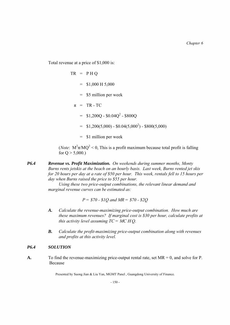
Total revenue at a price of $1,000 is:

TR = P Η Q = $1,000 Η 5,000 = $5 million per week π = TR - TC

= $1,200Q - $0.04Q2 - $800Q

= $1,200(5,000) - $0.04(5,0002) - $800(5,000) = $1 million per week

(Note: Μ2π/ΜQ2 < 0, This is a profit maximum because total profit is falling for Q > 5,000.)

P6.4 Revenue vs. Profit Maximization. On weekends during summer months, Monty

Burns rents jetskis at the beach on an hourly basis. Last week, Burns rented jet skis for 20 hours per day at a rate of $50 per hour. This week, rentals fell to 15 hours per day when Burns raised the price to $55 per hour.

Using these two price-output combinations, the relevant linear demand and marginal revenue curves can be estimated as:

P = $70 - $1Q and MR = $70 - $2Q

A. Calculate the revenue-maximizing price-output combination. How much are

these maximum revenues? If marginal cost is $30 per hour, calculate profits at this activity level assuming TC = MC Η Q.

B. Calculate the profit-maximizing price-output combination along with revenues

and profits at this activity level. P6.4 SOLUTION A. To find the revenue-maximizing price-output rental rate, set MR = 0, and solve for P.

Because

Demand Estimation


- 151 -

TR = P Η Q = ($70 - $1Q)Q = $70Q - $1Q2 MR = ΜTR/ΜQ MR = $70 - $2Q = 0 2Q = 70 Q = 35

At Q = 35, P = $70 - $1(35) = $35

Total revenue at a price of $35 is: TR = P Η Q = $35 Η 35 = $1,225 per day π = TR - TC

= $70Q - $1Q2 - $30Q

= $70(35) - $1(352) - $30(35) = $175 per day

(Note: Μ2TR/ΜQ2 < 0. This is a revenue-maximizing output level because total revenue is decreasing for output beyond Q > 35 hours.)

B. To find the profit-maximizing output level analytically, set MR = MC, or set Mπ = 0,

Chapter 6


- 152 -

and solve for Q. Because MR = MC $70 - $2Q = $30 2Q = 40 Q = 20

At Q = 20, P = $70 - $1(20) = $50

Total revenue at a price of $50 is: TR = P Η Q = $50 Η 20 = $1,000 per day π = TR - TC

= $70Q - $1Q2 - $30Q

= $70(20) - $1(202) - $30(20) = $400 per day

(Note: Μ2π/ΜQ2 < 0, This is a profit maximum because total profit is falling for Q > 20.)

P6.5 Linear Demand Curve Estimation. Anathema Printers, Inc., is a leading supplier of

high-speed color printers. Price and unit sales data per year are as follows:

2000

2001

2002

2003

2004 Price ($)

$9,000

$8,000

$6,000

$5,000

$3,000

Demand Estimation


- 153 -

Units sold 25,000 50,000 100,000 125,000 175,000

A. Complete the following table, and use these data to derive intercept and slope coefficients for the linear demand curve.

Year

Price

Quantity

ΜPric

e

ΜQuantity

Slope = ΜP/ΜQ

2000

$9,000

25,000

---

---

---

2001 8,000

50,000

2002 6,000

100,000

2003 5,000

125,000

2004 3,000

175,000

B. Assuming that demand conditions are held constant, use the preceding data to

plot a linear demand curve. P6.5 SOLUTION A. A linear demand curve is based on the assumption that a one-unit change in price

leads to a constant change in the quantity demanded. From the annual price/output data note that:

Year

Price

Quantity

ΜPrice

ΜQuantity

Slope = ΜP/ΜQ

2000 $9,000

25,000

---

---

---

2001 8,000

50,000

-$1,000

25,000

-0.04

2002 6,000

100,000

-2,000

50,000

-0.04

2003 5,000

125,000

-1,000

25,000

-0.04

2004 3,000

175,000

-2,000

50,000

-0.04

When a linear demand curve is written as:

P = a + bQ

a is the intercept and b is the slope coefficient. By definition, slope equals ΜP/ΜQ. From above:

Chapter 6


- 154 -

b = ΜP/ΜQ = -0.04.

Therefore, P = a - $0.04Q.

Under the assumption of a liner demand relation, each of the data points given in the table fall exactly along the linear demand curve. The value of the intercept term can be easily calculated using data for any of the data points given in the table. For example, using the 2004 data point where P = $3,000 and Q = 175,000,

P = a - $0.04Q $3,000 = a - $0.04(175,000) $3,000 = a - $7,000 a = $10,000

Therefore, in general: P = $10,000 - $0.04Q or Q = 250,000 - 25P B.

Demand Estimation


- 155 -

P6.6 Linear Demand Curve Estimation. Jackie Bouvier, the manager of a 100-unit

apartment building, knows from experience that all units will be occupied if rent is $900 per month. Bouvier also knows that, on average, one additional unit will go unoccupied for each $10 increase in the monthly rental rate.

A. Estimate the apartment rental demand curve assuming that it is linear and that

price is expressed as a function of output. B. Calculate the revenue-maximizing apartment rental rate. How much are these

maximum revenues.

C. With revenue maximization, what is the optimal number of vacant apartments? Explain your answer.

P6.6 SOLUTION A. When a linear demand curve is written as: P = a + bQ

a is the intercept, and b is the slope coefficient. By definition, slope equals ΜP/ΜQ. If one additional apartment unit will go unoccupied for each $10 increase in the monthly rental rate,

Chapter 6


- 156 -

b = ΜP/ΜQ = -10

Therefore, P = a - $10Q

Under the assumption of a liner demand relation, each of the data points for price and output fall exactly along the linear demand curve. Once the value of the slope coefficient is known, the value of the intercept term and the exact form of the demand curve can be easily calculated using any data point. For example, based on the fact that all apartments will be rented at a rental rate of $900 per month, Q = 100 and P = $900 is one data point. It follows that:

P = a - $10Q $900 = a - $10(100) $900 = a - $1,000 a = $1,900

Therefore, in general: P = $1,900 - $10Q B. To find the revenue-maximizing rental rate, set MR = 0, and solve for P. Because TR = P Η Q = ($1,900 - $10Q)Q = $1,900Q - $10Q2 MR = ΜTR/ΜQ MR = $1,900 - $20Q = 0 20Q = 1,900

Demand Estimation


- 157 -

Q = 95

At Q = 95, P = $1,900 - $10(95) = $950

Total revenue at a price of $950 is: TR = P Η Q = $950 Η 95 = $90,250

(Note: Μ2TR/ΜQ2 < 0. This is a rental-revenue maximizing output level because total ticket revenue is decreasing for output beyond Q > 95.)

C. In part B, it was determined that the revenue-maximizing apartment rental rate is P =

$950 per month. At that rental rate, Q = 95 apartments will be rented, and 5 units will remain vacant. Notice that while all apartments could be rented at a rental rate of P = $900, that rental rate would only generate $90,000 per month in rental revenues. At the higher $950 rate, an additional $250 in rental revenue is generated despite having 5 units remain vacant. Algebraically, the P = $900 per month is associated with MR < 0. Revenue maximization requires setting prices so that MR = 0, and solving for P.

P6.7 Identification Problem. Business is booming for Consulting Services, Inc. (CSI), a

local supplier of computer set-up consulting services. The company can profitably employ technicians as quickly as they can be trained. The average hourly rate billed by CSI for trained technician services and the number of billable hours (output) per quarter over the past six quarters are as follows:

Q-1

Q-2

Q-3

Q-4

Q-5

Q-6

Hourly rate ($) $20

$25

$30

$35

$40

$45

Billable hours 2,000

3,000

4,000

5,000

6,000

7,000

Quarterly demand and supply curves for CSI services are

Chapter 6


- 158 -

QD = 4,000 - 200P + 2,000T (Demand), QS = -2,000 + 200P (Supply),

where Q is output, P is price, T is a trend factor, and T = 1 during Q-1 and increases by one unit per quarter.

A. Express each demand and supply curve in terms of price as a function of output.

B. Plot the quarterly demand curves for the last six quarterly periods. (Hint: Let

T = 1 to find the Y intercept for Q-1, T = 2 for Q-2, and so on.)

C. Plot the CSI supply curve on the same graph.

D. What is this problem's relation to the identification problem? P6.7 SOLUTION A. Demand

QD = 4,000 - 200P + 2,000T

200P = 4,000 - QD + 2,000T

P = $20 - $0.005QD + $10T

Supply

QS = -2,000 + 200P

200P = 2,000 + QS

P = $10 + $0.005QS B.,C.

Demand Estimation


- 159 -

D. This problem illustrates the identification problem. If either the demand or supply

function is shifting while the other is stable, then the price/output data can be used to trace out the stable curve. Here the supply curve is stable while demand is growing rapidly (shifting to the right). Therefore, the price/output data given in the problem can be used to trace out the relevant supply curve.

P6.8 Correlation and Simple Regression. Market Research, Inc., has conducted a survey

to learn the relationship between income and age for a n = 15 sample of households in the affluent Minneapolis suburb of Eden Prairie, Minnesota. Survey results were as follows:

Age Income ($000)

32 81 33 86 33 87 37 92 38 94 40 99 41 102

Chapter 6


- 160 -

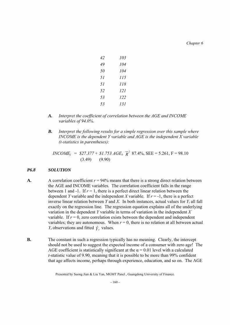
42 103 49 104 50 104 51 115 51 118 52 121 53 122 53 131

A. Interpret the coefficient of correlation between the AGE and INCOME

variables of 94.0%. B. Interpret the following results for a simple regression over this sample where

INCOME is the dependent Y variable and AGE is the independent X variable (t-statistics in parentheses):

INCOMEj = $27.377 + $1.753 AGEi, 2

R 87.4%, SEE = 5.261, F = 98.10 (3.49) (9.90) P6.8 SOLUTION A. A correlation coefficient r = 94% means that there is a strong direct relation between

the AGE and INCOME variables. The correlation coefficient falls in the range between 1 and -1. If r = 1, there is a perfect direct linear relation between the dependent Y variable and the independent X variable. If r = -1, there is a perfect inverse linear relation between Y and X. In both instances, actual values for Yt all fall exactly on the regression line. The regression equation explains all of the underlying variation in the dependent Y variable in terms of variation in the independent X variable. If r = 0, zero correlation exists between the dependent and independent variables; they are autonomous. When r = 0, there is no relation at all between actual Yt observations and fitted ˆ tY values.

B. The constant in such a regression typically has no meaning. Clearly, the intercept

should not be used to suggest the expected income of a consumer with zero age! The AGE coefficient is statistically significant at the α = 0.01 level with a calculated t-statistic value of 9.90, meaning that it is possible to be more than 99% confident that age affects income, perhaps through experience, education, and so on. The AGE

Demand Estimation


- 161 -

coefficient value of 1.7532 implies that a one year increase in AGE results in an average increase of $1,753 in the INCOME.

The 2R = 87.4 means that 87.4% of the variation in INCOME can be

explained using just the AGE independent variable. The F statistic of 98.10 means that this level of explained variation is statistically significant at more than the 99% confidence level, F = 98.10 > *

1,13, = .01F α = 9.07. The probability of encountering such a large F statistic when in fact no relation exists between these Y and X variables is less than 1%. The standard error of the estimate of 98.10 can be used to indicate the range within which actual income might be found for a customer with a given age. On average, actual income equals roughly Y ∀ (2 Η SEE) with 95% confidence, and Y ∀ (3 Η SEE) with 99% confidence.

P6.9 Multiple Regression. Colorful Tile, Inc., is a rapidly growing chain of ceramic tile

outlets that caters to the do-it-yourself home remodeling market. In 2004, 33 stores were operated in small to medium-size metropolitan markets. An in-house study of sales by these outlets revealed the following (standard errors in parentheses):

Q = 5 - 5P + 2A + 0.2I + 0.25HF (3) (1.8) (0.7) (0.1) (0.1) R2 = 93%, Standard Error of the Estimate = 6.

Here, Q is tile sales (in thousands of cases), P is tile price (per case), A is advertising expenditures (in thousands of dollars), I is disposable income per capita (in thousands of dollars), and HF is household formation (in hundreds).

A. Fully evaluate and interpret these empirical results on an overall basis using

R2, 2,R F-statistic and SEE information.

B. Is quantity demanded sensitive to Aown@ price?

C. Austin, Texas, was a typical market covered by this analysis. During 2004 in the Austin market, price was $5, advertising was $30,000, income was an average $50,000 per household, and the number of household formations was 4,000. Calculate and interpret the relevant advertising point elasticity.

D. Assume that the preceding model and data are relevant for the coming period.

Estimate the probability that the Austin store will make a profit during 2006 if total costs are projected to be $300,000.

Chapter 6


- 162 -

P6.9 SOLUTION A. (i) Coefficient of determination = R2 = 93%, implying that 93% of demand

variation is explained by the regression model. (ii) Corrected coefficient of determination = 2

R = R2 - (k - 1/n - k)(1 - R2) = 0.93 - (4/28)(1 - 0.93) = 0.92, implying that 92% of demand variation is explained by the regression model when both coefficient number, k, and sample size, N, are controlled for.

(iii) F statistic = (n - k/k - 1)(R2/1 - R2) = (28/4)(0.93/0.07) = 93 > F*4, 28, α = 0.01 = 4.07 implying one can reject the null hypothesis H0: b1 = b2 = b3 = b4 = 0 and conclude with 99% confidence that the dependent variables as a group explain a significant share of demand variation.

(iv) Standard error of the estimate = SEE = 6 implying that Q = Q ∀ 2.048 Η 6 with 95% confidence. Q = Q ∀ 2.763 Η 6 with 99% confidence. B. To determine whether quantity demanded depends upon Aown@ price, the question

must be asked: is bP 0? If bP 0, then evidence exists that sales do indeed depend upon price. For testing purposes, the null hypothesis one seeks to reject is the converse of the above question:

H0: bP = 0 (Two-tail test)

where,

|t| = P

P28, =0.01

b

5b| | = = 2.78 > = 2.763t1.8 ασ

which means it is possible to reject H0: bP = 0 with 99% confidence and conclude that yes, demand does seem sensitive to price.

C. Because Q = 5 - 5P + 2A + 0.2I + 0.25HF = 5 - 5(5) + 2(30) + 0.2(50) + 0.25(40)

Demand Estimation


- 163 -

= 60(000)

The point advertising elasticity is calculated as: εA = ΜQ/ΜA Η A/Q = 2 Η 30/60 = 1

Because εA = 1, a 1% increase in advertising will lead to commensurate percentage increase in demand.

D. Pr = 0.5 or 50%. To generate breakeven revenues of $300,000, Colorful Tile would

have to sell Q = TR/P = TC/P = $300,000/$5 = 60,000 cases. From part C, Q = 60(000). Because there is a 50/50 chance that actual sales

will be above or below this level, there is a 50/50 chance that the Austin store will make a profit when TC = $300,000.

P6.10 Multiplicative Demand Functions. Getaway Tours, Inc., has estimated the

following multiplicative demand function for packaged holiday tours in the East Lansing, Michigan, market using quarterly data covering the past four years (16 observations):

Qy = -1.10 0.5 3.8 2.5 1.85

y x y x10P P A A I R2 = 80%, Standard Error of the Estimate = 20

Here, Qy is the quantity of tours sold, Py is average tour price, Px is average price for some other good, Ay is tour advertising, Ax is advertising of some other good, and I is per capita disposable income. The standard errors of the exponents in the preceding multiplicative demand function are

A. Is tour demand elastic with respect to price?

B. Are tours a normal good?

C. Is X a complement good or substitute good?

y x y x IP P A A = 0.04, = 0.35, = 0.5, = 0.9, and = 0.45.b b b b b

Chapter 6


- 164 -

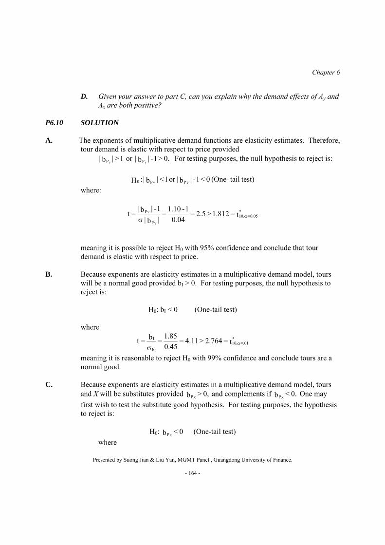
D. Given your answer to part C, can you explain why the demand effects of Ay and Ax are both positive?

P6.10 SOLUTION A. The exponents of multiplicative demand functions are elasticity estimates. Therefore,

tour demand is elastic with respect to price provided yP| | > 1b or

yP| | - 1 > 0.b For testing purposes, the null hypothesis to reject is:

where:

meaning it is possible to reject H0 with 95% confidence and conclude that tour demand is elastic with respect to price.

B. Because exponents are elasticity estimates in a multiplicative demand model, tours

will be a normal good provided bI > 0. For testing purposes, the null hypothesis to reject is:

H0: bI < 0 (One-tail test)

where

meaning it is reasonable to reject H0 with 99% confidence and conclude tours are a normal good.

C. Because exponents are elasticity estimates in a multiplicative demand model, tours

and X will be substitutes provided XP > 0,b and complements if

XP < 0.b One may first wish to test the substitute good hypothesis. For testing purposes, the hypothesis to reject is:

H0: XP < 0b (One-tail test)

where

Y Y0 P P: | | < 1 or | | - 1 < 0 (One- tail test)b bH

Y

Y

P *10, =0.05

P

| | - 1 1.10 - 1bt = = = 2.5 > 1.812 = t| | 0.04b

ασ

I

I *10, =.01

b

1.85bt = = = 4.11 > 2.764 = t0.45 α

σ

Demand Estimation


- 165 -

indicating it is reasonable to reject H0 with 90% confidence, and conclude tours and X are substitutes.

D. Both Aown@ and competitor advertising appear to increase sales. Although

relatively uncommon, this is not a rare occurrence. Advertising of substitutes can sometimes raise sales for competitor products due to beneficial spillover effects following increased customer awareness.

CASE STUDY FOR CHAPTER 6 Demand Estimation for Mrs. Smyth=s Pies Demand estimation for brand-name consumer products is made difficult by the fact that managers must rely on proprietary data. There simply is not any publicly available data which can be used to estimate demand elasticities for brand-name orange juice, frozen entrees, pies, and the like--and with good reason. Competitors would be delighted to know profit margins across a broad array of competing products so that advertising, pricing policy, and product development strategy could all be targeted for maximum benefit. Product demand information is valuable and jealously guarded.

To see the process that might be undertaken to develop a better understanding of product demand conditions, consider the hypothetical example of Mrs. Smyth's Inc., a Chicago-based food company. In early 2005, Mrs. Smyth's initiated an empirical estimation of demand for its gourmet frozen fruit pies. The firm is formulating pricing and promotional plans for the coming year, and management is interested in learning how pricing and promotional decisions might affect sales. Mrs. Smyth's has been marketing frozen fruit pies for several years, and its market research department has collected quarterly data over two years for six important marketing areas, including sales quantity, the retail price charged for the pies, local advertising and promotional expenditures, and the price charged by a major competing brand of frozen pies. Statistical data published by the U.S. Census Bureau (http://www.census.gov) on population and disposable income in each of the six market areas were also available for analysis. It was therefore possible to include a wide range of hypothesized demand determinants in an empirical estimation of fruit pie demand. These data appear in Table 6.2. Table 6.2 here

The following regression equation was fit to these data: Qit = b0 + b1Pit + b2Ait + b3PXit + b4Yit + b5Popit + b6Tit + uit

X

X

P *10, =0.10

P

0.50bt = = = 1.43 > 1.372 = t0.35 α

σ

Chapter 6


- 166 -

Q is the quantity of pies sold during the tth quarter; P is the retail price in dollars of Mrs. Smyth's frozen pies; A represents the dollars spent for advertising; PX is the price, measured in dollars, charged for competing premium-quality frozen fruit pies; Y is dollars of disposable income per capita; Pop is the population of the market area; T is the trend factor (2003-1 = 1, . . . , 2004-4 = 8); and uit is a residual (or disturbance) term. The subscript i indicates the regional market from which the observation was taken, whereas the subscript t represents the quarter during which the observation occurred. Least squares estimation of the regression equation on the basis of the 48 data observations (eight quarters of data for each of six areas) resulted in the estimated regression coefficients and other statistics given in Table 6.3. Table 6.3 here A. Describe the economic meaning and statistical significance of each individual

independent variable included in the Mrs. Smyth's frozen fruit pie demand equation. B. Interpret the coefficient of determination (R2) for the Mrs. Smyth's frozen fruit pie

demand equation. C. Use the regression model and 2004-4 data to estimate 2005-1 unit sales in the

Washington, DC-Baltimore, MD, market. D. To illustrate use of the standard error of the estimate statistic, derive the 95 per cent

and 99 per cent confidence intervals for 2005-1 unit sales in the Washington, DC-Baltimore, MD, market.

CASE STUDY SOLUTION A. The individual coefficients for the Mrs. Smyth's pie demand regression equation can

be interpreted as follows. The intercept term, 646,958, has no economic meaning in this instance; it lies far outside the range of observed data and obviously cannot be interpreted as the demand for Mrs. Smyth's frozen fruit pies when all the independent variables take on zero values. The coefficient for each independent variable indicates the marginal relation between that variable and sales of pies, holding constant the effect of all the other variables in the demand function. For example, the -127,443 coefficient for P, the price charged for Mrs. Smyth's pies, indicates that when the effects of all other demand variables are held constant, each $1 increase in price causes quarterly sales to decline by roughly 127,443 pies. Similarly, the 5.353 coefficient for A, the advertising and promotion variable, indicates that for each $1 increase in advertising during the quarter, roughly 5.353 additional pies are sold. Demand for Mrs. Smyth's pies rises by roughly 29,337 pies with every $1 increase in competitor prices, and a $1 increase in average disposable income per household

Demand Estimation


- 167 -

leads to roughly a 0.344-unit increase in quarterly pie demand. Similarly, a one person increase in the population of a given market area leads to a small 0.024-unit increase in quarterly pie demand. Finally, the coefficient for the trend variable indicates that pie demand is growing in a typical market by roughly 4,406 units per quarter. Mrs. Smyth's is enjoying secular growth in pie demand

Individual coefficients provide useful estimates of the expected marginal influence on demand following a one-unit change in each respective variable. However, they are only estimates. For example, it would be very unusual for a $1 increase in price to cause exactly a -127,443-unit change in the quantity demanded. The actual effect could be more or less. For decision-making purposes, it would be helpful to know if the marginal influences suggested by the regression model are stable or instead tend to vary widely over the sample analyzed. In general, if it is known with certainty that Y = a + bX, then a one-unit change in X will always lead to a b-unit change in Y. If b > 0, X and Y will be directly related; if b < 0, X and Y will be inversely related. If no relation at all holds between X and Y, then b = 0. Although the true parameter b is unobservable, its value is estimated by the regression coefficient ^b . If ^b = 10, a 1-unit change in X will increase Y by 10 units. This effect may appear to be large, but it will be statistically significant only if it is stable over the entire sample. To be statistically reliable, ^b must be large relative to its degree of variation over the sample.

In Mrs. Smyth's frozen fruit pie demand equation, the coefficient estimates for price (P), advertising (A), competitor price (PX) and population (Pop) are all more than twice as large as their respective standard errors. Therefore, it is possible to reject the hypothesis that each of these independent variables is unrelated to pie demand with 95 per cent confidence. These coefficient estimates suggest an especially strong relation between pie demand and the P, A, and Pop variables. Each of these coefficient estimates is over three times as large as its underlying standard error and therefore is statistically significant at the 99 per cent confidence level. Once the effects of these independent variables have been constrained, there is no additional independent influence noted for income (Y) or the time trend variable (T).

B. The coefficient of determination R2 = 0.896 or 89.6 percent indicates that the

regression model has explained 89.6 per cent of the total variation in pie demand. This is a very satisfactory level of explanation for the model as a whole. The corrected coefficient of determination 2

R = 0.881 or 88.1 per cent is a relatively modest downward adjustment from R2 = 89.6%; it suggests that the high level of explanatory power achieved by the regression model cannot be attributed to an overly small sample size. Finally, the F statistic is used to indicate whether a significant share of variation in the dependent variable has been explained by the

Chapter 6


- 168 -

regression model. The hypothesis actually tested is that the dependent Y variable is statistically unrelated to all the independent X variables included in the model. If this hypothesis cannot be rejected, variation explained by the regression is small. The critical value for F is denoted as

1 2,f f ,F where f1, the degrees of freedom for the numerator, equals k - 1, and f2, the degrees of freedom for the denominator, equals n - k. For example, the F statistic for this example involves f1 = k - 1 = 7 - 1 = 6, and f2 = n - k = 48 - 7 = 35 degrees of freedom. Also note that the calculated F6,35 = 58.86 > 3.47, the critical F6,30 value for the α = 0.01 or 99% confidence level. This means there is less than a 1% chance of observing such a high F statistic when there is no link between the dependent Y variable and the entire group of X variables. Given the ability to reject the hypothesis of no relation at the 99% confidence level, it will always be possible to reject this hypothesis at the lower, 95% and 90%, confidence levels.

C. To project the next quarter's sales of frozen fruit pies in the Washington, DC-

Baltimore, MD, market the company must simply enter expected values for each independent variable in the estimated demand equation. Mrs. Smyth's expects an average price for its pies of $7.36, advertising expenditures of $30,487. The prices of competing pies are expected to be $5.32; disposable income per capita is $41,989; population in the market area is 7,782,654 persons; and the quarter for which demand is being forecast is the ninth quarter in the model. Inserting the appropriate unit values into the demand equation results in an estimated demand of:

Q = 646957.817 - 127442.803(7.36) + 5.353(30,487) + 29,337.340(5.32) + 0.344(41,989) + 0.024(7,782,654) + 4,405.940(9) = 268,869 pies.

Mrs. Smyth's could forecast the total demand for its pies by forecasting sales in each of the six market areas, then summing these area forecasts to obtain an estimate of total pie demand. Using the results from the demand estimation model and data from each individual market, it would also be possible to construct a confidence interval for total pie demand based on the standard error of the estimate. (Note: Be sure to remember that 2005-1 is time period T = 9!)

D. Although 268,869 is the best estimate of pie demand for Washington, DC-Baltimore, MD,

during the 2005-1 period, it is highly unlikely that precisely this number of pies will actually be sold. Either more or less may be sold, depending on the effects of other

Demand Estimation


- 169 -

factors not explicitly accounted for in our pie demand estimation model. The standard error of the estimate is a very useful statistic because it allows us to construct a range or confidence interval within which actual sales are likely to fall. For example, sales can be projected to fall within a range of ∀ 2 standard errors of the 268,869 expected sales level with a confidence level of 95 per cent . The standard error of the estimate for the Mrs. Smyth's pie demand-estimation model is roughly 60,700 pies. Therefore, an interval of ∀ 2(60,700) or ∀ 121,400 pies around the expected sales of 268,869 pies represents the 95 per cent confidence interval. This means that one can predict with a 95 per cent probability of being correct that sales of Mrs. Smyth's pies during the next quarter in the Washington, DC-Baltimore, MD, area will lie in the range from 147,469 to 390,269 pies. Assuming that the hypothesized values for the various independent variables are correct, there is only a 5 per cent chance that actual sales in the Washington, DC-Baltimore, MD, market during the coming period will fall outside this range. Similarly, there is a 99 per cent chance that actual sales will fall in the range of 268,869 ∀ 3(60,700), or between 86,769 and 450,969 pies, and only a 1 per cent chance that actual sales will fall outside this range.

Solutions Chapter 5

Documents

Transcript of Solutions Chapter 5