Johan LarssonUniversity of Maryland

PSAAP-3 Kickoff MeetingAug 18-19, 2020

Solution-verification, grid-adaptation and uncertainty quantification for chaotic turbulent flow problems

Ivan Bermejo-MorenoUniversity of Southern California

Qiqi WangMIT

𝑢

Motivation and target problems

PDEs exhibiting turbulence – chaotic, truly multiscale (broadband) solutions

2

Supernovae explosions

Shock/turbulence interactions

Rayleigh-Taylor mixing

Typically with many problem parameters: Reynolds number, initial disturbance, geometry, fluid properties, model form and coefficients, …

In general, turbulence + other physics effects (shocks, chemistry, …) –this work is focused on the turbulence

Supersonic combustion

The need for the sensitivity gradient ∇𝐽 in UQ of turbulent flows

• 𝒪 100 or more parameters – must avoid ”curse-of-dimensionality” (e.g., no polynomial chaos).

• Different engineering challenges require different levels of UQ:a) Approximate error barsb) Confidence intervalsc) Full pdf, long-tail events,…

• Error attribution – ∇𝐽 provides direct information

• Estimating the effects of grid-induced errors – requires ∇𝐽 due to the extremely high dimensionality

3

Approximate 𝜎( sufficient Sensitivity (∇𝐽) is sufficient Approximate 𝜎(, approx. pdf With ∇𝐽, gradient-enhanced KrigingMust sample With ∇𝐽, can focus sampling

0.0 0.4 0.8 1.2 1.6 2.0�P/�Psep

0

1

2

3

4

5

6

Lin

t/(�

⇤ g3)

0.0 0.4 0.8 1.2 1.6�P/�P 0

sep

0

1

2

3

4

5

6

Lin

t/(�

⇤ g3)

(a) (b)

Sample VVUQ problem:Does DNS (red/blue/black) agree with experiment (green)?

2. Develop algorithms that use the sensitivity gradient (of different levels of accuracy) to perform:• uncertainty estimation• error attribution• grid adaptation

Specific objectives:1. Develop algorithms for computing the sensitivity gradient 𝛁𝑱 for chaotic turbulence problems

Consider methods at different levels of accuracy and cost

Project objectives

Main goal: to develop a mathematical foundation for VVUQ of PDEs that exhibit chaotic/broadband dynamics

4

- how large is the error in 𝐽?- what factors contribute the most to my estimated error/uncertainty?- how to design/refine grid to optimally reduce the error in 𝐽?

∇𝐽 ≡ gradient in parameter space of a QoI 𝐽

Focus application: turbulent boundary layer over flat plate, with varying pressure gradients

The developed methods will be applicable to a wide range of chaotic problems

Overall approach

The key challenge: In realistic chaotic/broadband (turbulence) problems with many parameters, computing ∇𝐽 is only affordable via adjoints – but the adjoint equations diverge exponentially, and the available solutions (shadowing, ensembles of short-duration adjoints) are infeasibly costly or inapplicable in general.

5

Overall approach:1. Develop multiple methods to compute ∇𝐽 stemming from different approximations and trade-offs:

a) Methods starting from chaos-theory (shadowing and others)b) Methods starting from physics-inspired reduced-order modelingc) Methods combining ideas from these philosophically different approaches

2. Local error estimation, for use in both uncertainty estimation and grid-adaptation3. Compare these methods on a validation / benchmark problem – learn about strengths, weaknesses,

inherent limitations, possible improvements, ...

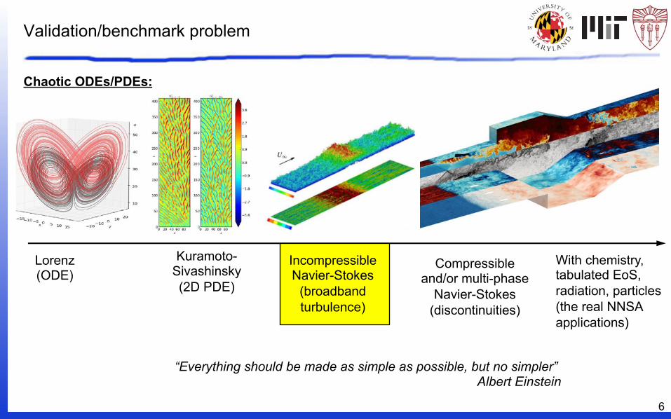
Validation/benchmark problem

6

Chaotic ODEs/PDEs:

Lorenz(ODE)

Kuramoto-Sivashinsky(2D PDE)

Incompressible Navier-Stokes

(broadband turbulence)

Compressible and/or multi-phase

Navier-Stokes(discontinuities)

With chemistry, tabulated EoS, radiation, particles(the real NNSA applications)

“Everything should be made as simple as possible, but no simpler”Albert Einstein

Our choice: Flat-plate turbulent boundary layer with spatial pressure gradient• Space of parameters for sensitivity studies includes:

• Natural parameters – can be highly controlled in our own reference simulations:• Reynolds number• State of incoming boundary layer (thickness + mean & turbulent wall-normal profiles)• Spatial mean pressure profiles in streamwise and spanwise directions

• Modeling parameters (evaluation of epistemic uncertainties):• Subgrid-scale (SGS) model• Wall model (future studies)

• Quantities of Interest:• Drag force streamwise & spanwise• Size of separation bubble

Validation/benchmark problem

7

wall-normal gradient of streamwise velocity

𝑄-criterion isosurfaces

Coleman et al (2018)

wall-distance

𝜕𝑢/𝜕𝑦

𝑢

𝑥𝑦

𝑧Flat plate boundary layer with non-zero pressure gradient

Sensitivity divergence in long-time-averaged chaotic systems1

8

Instantaneous QoI

time

Time-averaged QoI

Chaotic problems have unstable manifolds, which by definition cause divergence of the linearized initial-value problem

1 e.g., Lea et al (Tellus 2000)

One solution: Least squares shadowing (LSS)1

9

Instantaneous QoI

time

Time-averaged QoI

A “shadow trajectory” is defined to stay close to the reference solution at all times, while satisfying the governing equation

1 Wang (SIAM 2014)

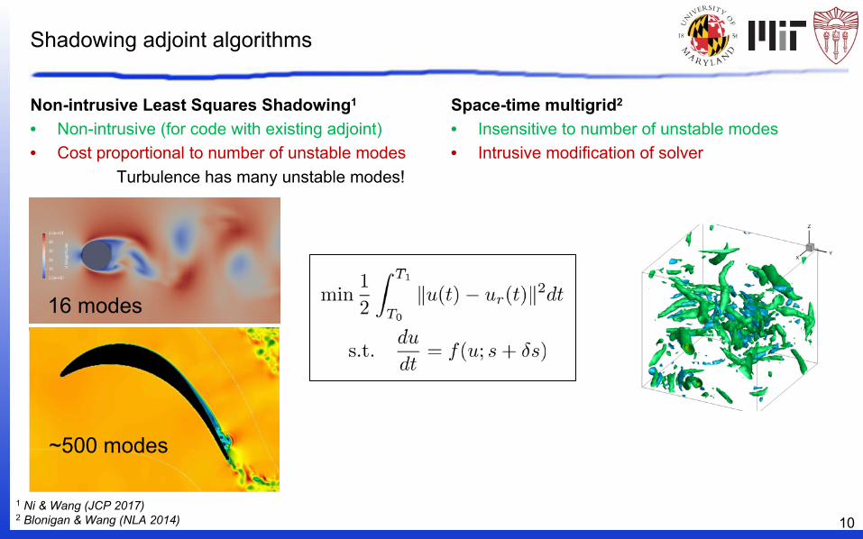
Shadowing adjoint algorithms

Non-intrusive Least Squares Shadowing1

• Non-intrusive (for code with existing adjoint)• Cost proportional to number of unstable modes

Turbulence has many unstable modes!

10

16 modes

~500 modes

Space-time multigrid2

• Insensitive to number of unstable modes• Intrusive modification of solver

1 Ni & Wang (JCP 2017)2 Blonigan & Wang (NLA 2014)

Cost reduction ideas for shadowing algorithm

Theorem: a shadowing tangent solution can be found within the affine space of:

1. the tangent restricted to the stable subspace, and2. the span of all unstable modes

Example: low-Re flow over a cylinder

Lyapunov exponents

Cost reduction ideas for shadowing algorithm

Theorem: a shadowing tangent solution can be found within the affine space of:

1. the tangent restricted to the stable subspace, and2. the span of all unstable modes

Observation: Many unstable modes can have the same high-wavenumber content and differ from each other only in their “modulation”, a low-wavenumber multiplicative factor.

Hypothesis: Cost reduction can be achieved through computing multiple unstable modes by solving a single tangent equation, then apply different low-wavenumber modulations to the solution.

In addition: There are other approaches (beyond shadowing) based on similar ideas from chaos theory – we will pursue these too.

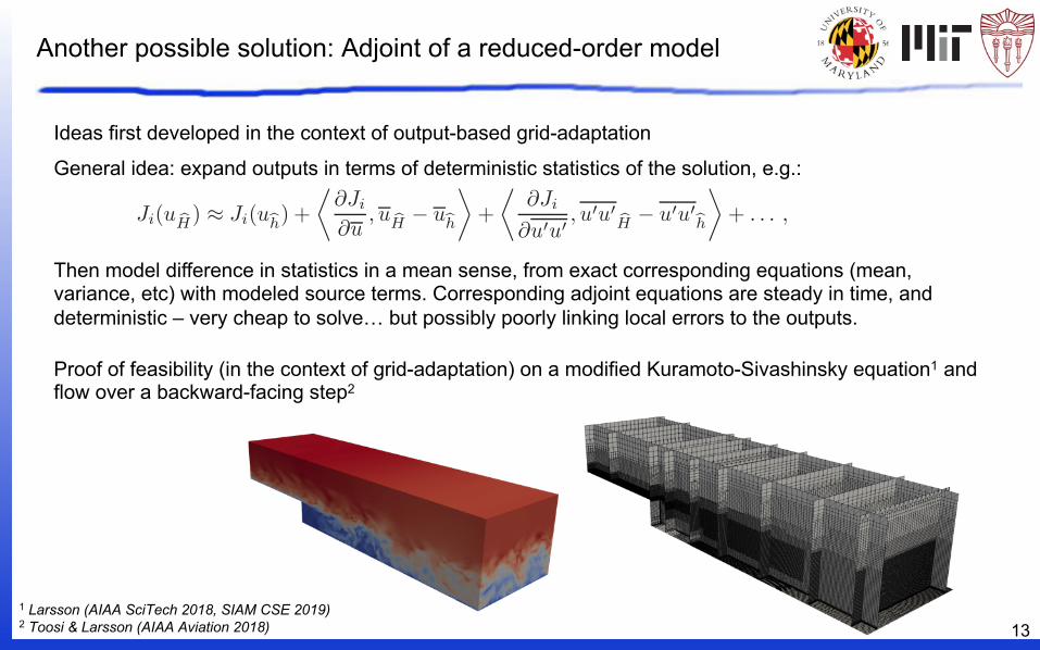
Another possible solution: Adjoint of a reduced-order model

13

estimate is still not a bound), but it may diminish the problem in practice if one chooses to construct thefirst GH through refinement: in that case, even if the initial grid is exceedingly coarse, it is hard to imagine auniform refinement by a factor of 2 or so having no real effect on the outputs. Therefore, we may hypothesizethat the proposed formulation could be useful even for non-chaotic problems.

Having argued for a new formulation of the grid-adaptation problem in this section, we proceed byproposing one possible approach of solving it.

3. One approach to solving the verification-driven grid-adaptation problem

In order to solve the new grid-adaptation problem, the heart of the matter is the need for a link betweena candidate grid-spacing ∆h(x, t) and the difference in simulation outputs |Ji(uH) − Ji(uh)| that it wouldproduce (after the uniform coarsening). Even for chaotic problems, outputs must be deterministic in orderto be meaningful: they could be means and variances of the solution, or conditional averages, or perhapsmore general moments of a probability density function. But the outputs would necessarily contain someaveraging to make them deterministic and thus meaningful.

The idea here is therefore to expand the outputs not in terms of the solution itself but rather in terms ofdeterministic statistics of the solution. The ideal choice of statistics (or averages) to include in the expansionis probably application- and output-specific; to illustrate the concept, we expand in terms of the mean u(x, t)and variance u′u′(x, t) here, as

Ji(uH) ≈ Ji(uh) +

⟨∂Ji∂u

, uH − uh

⟩

+

⟨∂Ji∂u′u′

, u′u′

H − u′u′

h

⟩

+ . . . , (7)

with the dots implying that additional (or other) quantities could be included.Note that averaging could be performed in multiple ways, including ensemble- or phase-averaging; thus

the averaged quantities may still depend on t.We emphasize that the choice of expanding in terms of u and u′u′ is just one choice – for outputs that

are more related to other types of statistics, those could be used instead. Similarly, there is no limit on thenumber of terms in the expansion (other than computational cost). Having said this, there are probablymany applications where the most important outputs are strongly related to either the mean or variance ofthe solution. In the interest of conciseness, in the following we assume that the expansion (7) is accurate andreasonable. Obviously, for a three-dimensional problem, we would expand in terms of all components ui andu′

iu′

j.The fact that the outputs Ji are statistics of an underlying chaotic solution also implies that they are

necessarily polluted by an error due to finite sampling (e.g., too few ensemble averages, or too short time-averaging). This error affects both the verification and adaptation criteria (Eqns. 5 and 6), and turns theminto de facto probabilistic hypothesis tests. This issue is left for future work, and we assume that statisticsare perfectly sampled here.

As is the case in classic grid-adaptation (the adjoint-weighted residual method), the inner products inEqn. (7) are most efficiently computed using adjoints. To find these adjoints, we must first derive linearizedequations for small perturbations in u(x, t) and u′u′(x, t).

3.1. Equations for small perturbations of the mean and variance

Averaging the exact evolution equation (1) yields

N (u(x, t)) ≡ M(

u(x, t), u′u′(x, t), . . .)

= 0 ,

which is an equation for the mean u(x, t) that contains unclosed higher-order terms. Exactly which higher-order terms depends on the nature of the nonlinearity in N ; in this work, we assume a quadratic nonlinearity,for which M(u, u′u′) = 0. This assumption is true for the incompressible Navier-Stokes equations and theapplications we consider below.

If we instead average the coarse-grained and discretized equation (3), we get

M(

uh, u′u′h

)

= Sh , (8)

6

General idea: expand outputs in terms of deterministic statistics of the solution, e.g.:

Then model difference in statistics in a mean sense, from exact corresponding equations (mean, variance, etc) with modeled source terms. Corresponding adjoint equations are steady in time, and deterministic – very cheap to solve… but possibly poorly linking local errors to the outputs.

Ideas first developed in the context of output-based grid-adaptation

Proof of feasibility (in the context of grid-adaptation) on a modified Kuramoto-Sivashinsky equation1 and flow over a backward-facing step2

1 Larsson (AIAA SciTech 2018, SIAM CSE 2019)2 Toosi & Larsson (AIAA Aviation 2018)

Adjoint of a reduced-order model

In this project, use this general idea of expanding the output in terms of deterministic statistics

14

estimate is still not a bound), but it may diminish the problem in practice if one chooses to construct thefirst GH through refinement: in that case, even if the initial grid is exceedingly coarse, it is hard to imagine auniform refinement by a factor of 2 or so having no real effect on the outputs. Therefore, we may hypothesizethat the proposed formulation could be useful even for non-chaotic problems.

Having argued for a new formulation of the grid-adaptation problem in this section, we proceed byproposing one possible approach of solving it.

3. One approach to solving the verification-driven grid-adaptation problem

In order to solve the new grid-adaptation problem, the heart of the matter is the need for a link betweena candidate grid-spacing ∆h(x, t) and the difference in simulation outputs |Ji(uH) − Ji(uh)| that it wouldproduce (after the uniform coarsening). Even for chaotic problems, outputs must be deterministic in orderto be meaningful: they could be means and variances of the solution, or conditional averages, or perhapsmore general moments of a probability density function. But the outputs would necessarily contain someaveraging to make them deterministic and thus meaningful.

The idea here is therefore to expand the outputs not in terms of the solution itself but rather in terms ofdeterministic statistics of the solution. The ideal choice of statistics (or averages) to include in the expansionis probably application- and output-specific; to illustrate the concept, we expand in terms of the mean u(x, t)and variance u′u′(x, t) here, as

Ji(uH) ≈ Ji(uh) +

⟨∂Ji∂u

, uH − uh

⟩

+

⟨∂Ji∂u′u′

, u′u′

H − u′u′

h

⟩

+ . . . , (7)

with the dots implying that additional (or other) quantities could be included.Note that averaging could be performed in multiple ways, including ensemble- or phase-averaging; thus

the averaged quantities may still depend on t.We emphasize that the choice of expanding in terms of u and u′u′ is just one choice – for outputs that

are more related to other types of statistics, those could be used instead. Similarly, there is no limit on thenumber of terms in the expansion (other than computational cost). Having said this, there are probablymany applications where the most important outputs are strongly related to either the mean or variance ofthe solution. In the interest of conciseness, in the following we assume that the expansion (7) is accurate andreasonable. Obviously, for a three-dimensional problem, we would expand in terms of all components ui andu′

iu′

j.The fact that the outputs Ji are statistics of an underlying chaotic solution also implies that they are

necessarily polluted by an error due to finite sampling (e.g., too few ensemble averages, or too short time-averaging). This error affects both the verification and adaptation criteria (Eqns. 5 and 6), and turns theminto de facto probabilistic hypothesis tests. This issue is left for future work, and we assume that statisticsare perfectly sampled here.

As is the case in classic grid-adaptation (the adjoint-weighted residual method), the inner products inEqn. (7) are most efficiently computed using adjoints. To find these adjoints, we must first derive linearizedequations for small perturbations in u(x, t) and u′u′(x, t).

3.1. Equations for small perturbations of the mean and variance

Averaging the exact evolution equation (1) yields

N (u(x, t)) ≡ M(

u(x, t), u′u′(x, t), . . .)

= 0 ,

which is an equation for the mean u(x, t) that contains unclosed higher-order terms. Exactly which higher-order terms depends on the nature of the nonlinearity in N ; in this work, we assume a quadratic nonlinearity,for which M(u, u′u′) = 0. This assumption is true for the incompressible Navier-Stokes equations and theapplications we consider below.

If we instead average the coarse-grained and discretized equation (3), we get

M(

uh, u′u′h

)

= Sh , (8)

6

and expand the range of accuracy/cost possibilities:• Where to truncate the expansion? After mean, (co-)variances, higher-order?• How to model unclosed terms? Inferred eddy-viscosity and analogously for higher moments?• How does the accuracy depend on the flow, the parameter, and the QoI?• Consider averages other than in time, for use in unsteady problems – e.g., applicable to Rayleigh-Taylor etc

Consider complexity-reduction that retains some chaotic character but with very few unstable modes –could then be combined with the chaos-theory-based methods?

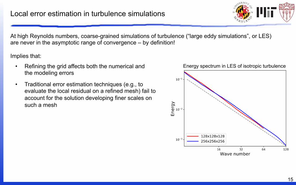
Local error estimation in turbulence simulations

At high Reynolds numbers, coarse-grained simulations of turbulence (“large eddy simulations”, or LES) are never in the asymptotic range of convergence – by definition!

15

Energy spectrum in LES of isotropic turbulence• Refining the grid affects both the numerical and the modeling errors

• Traditional error estimation techniques (e.g., to evaluate the local residual on a refined mesh) fail to account for the solution developing finer scales on such a mesh

Implies that:

Local error estimation in turbulence simulations

Approaches:

16

Actual LES Frozen 𝑢2u0iu

0j

<latexit sha1_base64="(null)">(null)</latexit><latexit sha1_base64="(null)">(null)</latexit><latexit sha1_base64="(null)">(null)</latexit><latexit sha1_base64="(null)">(null)</latexit>

increases

⌧

model

ij ⇠ C�2

����@ui

@xj

����@ui

@xj<latexit sha1_base64="(null)">(null)</latexit><latexit sha1_base64="(null)">(null)</latexit><latexit sha1_base64="(null)">(null)</latexit><latexit sha1_base64="(null)">(null)</latexit>

�<latexit sha1_base64="(null)">(null)</latexit><latexit sha1_base64="(null)">(null)</latexit><latexit sha1_base64="(null)">(null)</latexit><latexit sha1_base64="(null)">(null)</latexit> decreases

increases

unchanged

decreases

unchanged@ui/@xj<latexit sha1_base64="(null)">(null)</latexit><latexit sha1_base64="(null)">(null)</latexit><latexit sha1_base64="(null)">(null)</latexit><latexit sha1_base64="(null)">(null)</latexit>

Grid-refinement of LES with an eddy-viscosity model:

1. Traditional residual-based: interpolate solution onto refined grid, evaluate the residual. But does this estimate what would actually happen on a refined grid, where smaller scales would develop?

3. “Coarse-graining consistency” error estimation

2. Estimation of the time-averaged error by comparing averages (and co-variances, etc) on different grids – natural consequence of the “averaged adjoint” approach to sensitivity.• Works in channel flow and backward-facing step flow, but what about more general types of flows?

Software integration (and essentially the overall work plan...)

DNS/LES flat-plate flow (primal) solver Chaos-theory-based approaches

• Cartesian, co-located structured grid• Incompressible Navier-Stokes• Finite difference (2nd – 6th order)• Fractional step time integration • DFT, pencil-based, null-space

pressure Poisson solver Adjoint of ROM approaches

• Adjoint of non-chaotic (RANS) averaged forward equations

• Eddy-viscosity inference from LES data

• Higher-order statistics based

Local error estimators

• Numerical residual• Small-scale resolved energy • Solution differences in

everywhere-dissimilar grids

Grid convergence and adaptation

Forward problem UQ and sensitivity analysis Error and solution verification

• Setup of simulation parameter sweeps• Ensemble jobs, and run pipeline.

UMDMITUSC

Multi-solver software framework for integrated VVUQ on high-fidelity simulation of chaotic, turbulent flow

1) Interface with existing resource manager frameworks (e.g., Flux)2) MPI-based embedded many-run execution within single job submission

LES mode

DNS mode

• !! forward DNS simulations for perturbed input parameters.

Verification of methodology with DNS `truth’

• Finite-difference based sensitivity and error estimation

• Comparison and assessment of VVUQ methodology

• Space-time multigrid type solvers• Non-intrusive solvers, utilizing

Jacobian• Phase-space based solvers

Exascale approach:Kokkos, Trilinos

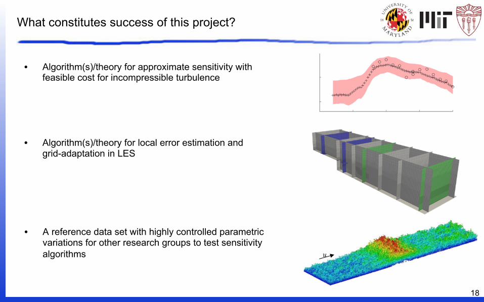
What constitutes success of this project?

• Algorithm(s)/theory for approximate sensitivity with feasible cost for incompressible turbulence

18

𝑢

• Algorithm(s)/theory for local error estimation and grid-adaptation in LES

• A reference data set with highly controlled parametric variations for other research groups to test sensitivity algorithms