
Solution of Linear Optimization Problems using a Simplex like
51
2006:285 CIV MASTER'S THESIS Solving Linear Optimization Problems using a Simplex Like Boundary Point Method in Dual Space Per Bergström Luleå University of Technology MSc Programmes in Engineering Engineering Physics Department of Mathematics 2006:285 CIV - ISSN: 1402-1617 - ISRN: LTU-EX--06/285--SE
Transcript of Solution of Linear Optimization Problems using a Simplex like

2006:285 CIV
M A S T E R ' S T H E S I S
Solving Linear Optimization Problemsusing a Simplex Like Boundary Point
Method in Dual Space
Per Bergström
Luleå University of Technology
MSc Programmes in Engineering Engineering Physics
Department of Mathematics
2006:285 CIV - ISSN: 1402-1617 - ISRN: LTU-EX--06/285--SE

Solving Linear Optimization Problems using a
Simplex like boundary point method in dual
space
by
Per Bergstrom
Department of Mathematics
Lulea University of Technology
SE-971 87 Lulea
Sweden
October 1, 2006


Abstract
This thesis treats an algorithm that solves linear optimization problems. Thealgorithm is based on a similar idea as the simplex method but in this algorithmthe start value also might be an inner point or a boundary point at the feasibleregion. The start value does not necessarily have to be a corner point that thesimplex algorithm demands. The algorithm solves problems in standard form.That means that the constraints are with equality and every variable must bepositive. The algorithm operates in the dual space to the original problem. Duringthe progress of the algorithm the iteration points will be on the boundary at thefeasible region to the dual problem and finally end up in a corner. Afterwardsthe iteration values go from corner to corner until finally the optimum is reached,just like the simplex algorithm. The expected time to solve linear optimizationproblems with this algorithm seems to be polynomial in time with respect to thesize of the problem, thought the worst case behavior has not been analyzed. Ifthe last iteration value is just an approximate solution to the dual problem thealgorithm will transfer it to a quite good approximation to the primal problem.Much of the development in this thesis is a continuation of a similar algorithmwhich was done one year ago.
In the introduction and in the second chapter different forms of linear optimiza-tion problems are described. The algorithm is implemented in Matlab R© and thecode can be find in the appendices of this paper. There are also different versions,which solve different types of problems. One for general problems and one fornetwork flow problems.
3

Acknowledgments
First of all I would like to thank my supervisor, associate professor Ove Edlund.He has taken his doctor’s degree in scientific computing. A majority part of hisdoctoral thesis deals with linear programming. The interested reader who wantsto read it can find it on the web. There is a link to Ove’s thesis in the referencesof this thesis, in fact reference number [1]. It was perfect to have a supervisor likeOve when experiment with and writing about linear programming. It is alwaysgood to have an experienced supervisor in his own subject when doing research.
This thesis has been time consuming. At least it took a long while from startuntil finish. Before I finished my master thesis I was offered an interesting traineejob. That was a trainee job at the Swedish company Tomlab1, which is the world-
wide leading company in optimization solvers for Matlab R© and LabVIEWTM
.The company has offices in Vasteras (Sweden) and San Diego (USA, CA), and Iwas placed in San Diego. It was very exciting to live in another part of the worldfor a while than northern Sweden where I was born and usually live. The traineejob at Tomlab had no direct connection with this thesis, but the job gave meunderstanding in how extremely important optimization is for the society today.It also gave me lots of experiences in computer science and last but not least, itgave me knowledge in how it is to work in the industry. However, it was not ahard decision to accept the job offer from Tomlab, even if I was forced to finishthis thesis during the lovely Swedish summer.
Lulea, October 1, 2006
Per Bergstrom
1http://www.tomlab.biz/
4

Table of Contents
List of Tables . . . . . . . . . . . . . . . . . . . . . . . . . . . . . . . . 6
1. Introduction . . . . . . . . . . . . . . . . . . . . . . . . . . . . . . 7
2. Linear Optimization and Sparse Matrices . . . . . . . . . . . . 92.1. Example 1. A Transportation Problem . . . . . . . . . . . . 92.2. Example 2. Relay swimming race . . . . . . . . . . . . . . . 132.3. Example of network flow problem . . . . . . . . . . . . . . . 15
3. Simplex method . . . . . . . . . . . . . . . . . . . . . . . . . . . . . 22
4. Simplex boundary method . . . . . . . . . . . . . . . . . . . . . . 234.1. An improvement . . . . . . . . . . . . . . . . . . . . . . . . 244.2. Dual problem . . . . . . . . . . . . . . . . . . . . . . . . . . 24
5. Test result . . . . . . . . . . . . . . . . . . . . . . . . . . . . . . . 265.1. Dense matrices . . . . . . . . . . . . . . . . . . . . . . . . . 265.2. Network flow problems . . . . . . . . . . . . . . . . . . . . . 275.3. Netlib test problems . . . . . . . . . . . . . . . . . . . . . . 29
6. Conclusion . . . . . . . . . . . . . . . . . . . . . . . . . . . . . . . . 30
7. Other methods . . . . . . . . . . . . . . . . . . . . . . . . . . . . . 31
Appendix A. Sketch of a convergence proof . . . . . . . . . . . 32
Appendix B. lpmin.m . . . . . . . . . . . . . . . . . . . . . . . . . . . . 33
Appendix C. lpmin flow.m . . . . . . . . . . . . . . . . . . . . . . . . . 44
References . . . . . . . . . . . . . . . . . . . . . . . . . . . . . . . . . . 49
5

List of Tables
Table 2.1. The yearly capacities and requirements in suitable units. . . . 9Table 2.2. Unit costs for supplying each customer from each supplier. . 9Table 2.3. The swimmers personal best expressed in seconds. . . . . . . 13
Table 5.1. Comparison between two different algorithms. m is the numberof equality constraints and t is measured in seconds. . . . . . . . . . 26
Table 5.2. Comparison between two different algorithms. m is the numberof equality constraints and t is measured in seconds. . . . . . . . . . 27
Table 5.3. Results from comparison with problem from simsys sparse.m is the number of equality constraints and t is measured in seconds. 28
Table 5.4. Results from comparison with problem from simsys sparse2.m is the number of equality constraints and t is measured in seconds. 28
Table 5.5. Results from comparison with problem from Netlib. t is mea-sured in seconds. . . . . . . . . . . . . . . . . . . . . . . . . . . . . . 29
6
1. Introduction
This Master Thesis is a sequel to a D-level thesis that was done one year ago. Theresult from that was so good, enough to make a continuation possible, a Masterthesis, on the same theme. The algorithm in the D-level thesis solves problem inone mathematical form, not a usual form in applied problems. That’s the goalin this thesis, to write the code suited for applied problems. In the beginning ofthis thesis some applied problems will be described. Two different terms are used,linear programming and linear optimization, but they describe the same thing.
First of all, something about linear programming and its history must be men-tioned. For the readers who are not familiar with the subject, it can be said thatit all started for about 60 years ago, during World War II. At least, lots of thingsin the area of subject took shape at that time. Of course, lots of persons were in-volved into developing and improvement of solving linear programming problems,but there is one who has a special influence and has been acknowledged as thefounder of the first efficient solving algorithm, the simplex method. His name isGeorge Dantzig. George worked with military planning in Pentagon for the U.S.Air Force during World War II. He was expert in solving planning problems with adesk calculator. It was then it all started. Developing mathematical models werenot the only thing he did, he also developed an efficient solver to the problems.The method is called the simplex method. Since that time mathematical planninghas been spread to more applications than military planning. In the beginningof the book ”Linear programming and extensions”, which is written by GeorgeDantzig, reference [2], Dantzig gives examples of linear programming problemsand also the origins to linear programming models.
Today it is an important tool in many industrial applications and financialand economical science. The development of models has led to larger and largerproblems. Problems with a size of millions of variables are not unrealistic. Seefor example reference [3], where the authors describe and solve a problem withmillions of variables, and they make use of a linear programming solver. Suchlarge problems will take very long time to solve. With that size of problems it isvery important what kind of solving method you are using. It also may bee goodidea to make use of a supercomputer. Then it is good to have an algorithm thatis efficient to use on a parallel computer.
Until the middle of the 80’s the simplex method was with no doubt the leadingsolver. Then there came new generation solvers called inner point methods. Thedifference between the inner point methods and the simplex method is that in thesimplex method all the iteration points are in corners to the feasible region. Inthe inner point method all the iteration points are inside the feasible region. Forvery large problems the simplex method might be very time consuming. That isbecause of the numbers of corners to the feasible region grow exponential to thesize of the problem. However, the inner point method might be unstable because ofall the numerical troubles that might occur. So different problems claim different
7

1. Introduction
solvers. For one type of problem one solver is the best, and for another type ofproblem another solver is the best. Which solver is the best depends on manythings. One thing is clear, when solving large linear programming problems, itmight be an advantage to have many solvers to choose from.
In the following text linear programming will be abbreviated as LP.
8

2. Linear Optimization and Sparse Matrices
In applied linear programming the matrix will often be huge and sparse. Thesparse pattern arises because of weak relations between all the decision variables.Every variable just has direct connection with a couple of other variables amongperhaps thousands of them. A detailed example of this follows in section 2.3. Inthis chapter examples of linear programming problems from the reality will bedescribed. There is lot of literature where you can find examples of applied linearprogramming. For example, see [4],[5] or [6].
One of many types of problems is the transportation problem. In [4] Williamsgives an example of such a problem. At page 73 you can find the following example.
2.1. Example 1. A Transportation Problem
Three suppliers (S1,S2,S3) are used to provide four customers (T1,T2,T3,T4) withtheir requirements for a particular commodity over a year. The yearly capacities ofthe suppliers and requirements of the customers are given in table 2.1 (in suitableunits).
Table 2.1. The yearly capacities and requirements in suitable units.
Suppliers S1 S2 S3
Capacities (per year) 135 56 93Customers T1 T2 T3 T4
Requirements (per year) 62 83 39 91
The unit costs for supplying each customer from each supplier are given in table2.2 (in £/unit).
Table 2.2. Unit costs for supplying each customer from each supplier.
CustomersT1 T2 T3 T4
S1 132 - 97 103Suppliers S2 85 91 - -
S3 106 89 100 98
A dash indicates the impossibility of certain suppliers for certain depots or cus-tomers.
The total capacity of the suppliers is greater than the requirement of the cus-tomers. To get an easier structure in the problem you can introduce a new cus-tomer (it is called a dummy customer) with requirement 9 units per year. With
9

2. Linear Optimization and Sparse Matrices
the new dummy customer the total capacity of the suppliers is equal to the re-quirement of the customers.
The problem can be viewed in a graph. Se figure 2.1.
Figure 2.1. Graph for problem in example 1.
This problem can be formulated to a LP model by introducing variables xij torepresent the quantity of the commodity sent from Si to Tj in a year. The resultantmodel is (2.1).
10

2. Linear Optimization and Sparse Matrices
min
132x
11+
97x
13+
103x
14+
85x
21+
91x
22+
106x
31+
89x
32+
100x
33+
98x
34
subje
ctto
−x11−x
13−x
14−x
15
=−1
35−x
21−x
22−x
25
=−5
6−x
31−x
32−x
33−x
34−x
35
=−9
3x
11
+x
21
+x
31
=62
+x
22
+x
32
=83
x13
+x
33
=39
x14
+x
34
=91
x15
+x
25
+x
35
=9
xij
≥0,∀i
,j
(2.1
)
11

2. Linear Optimization and Sparse Matrices
If the dummy customer T5 was not introduced the three first equalities had beeninequalities. As you can see the model has a very special structure.
Another type of problem is the assignment problem. In [7] the authors give anexample of an assignment problem.
12

2. Linear Optimization and Sparse Matrices
2.2. Example 2. Relay swimming race
Before every Olympic Game or big competition the national swimming team man-ager gets the commission to take out the best team in relay swimming 4x100 metermedley. Medley consists of the sections backstroke, butterfly, breaststroke andfreestyle. At the Olympic Games in Sidney the national women’s team managerhad to choose from among six swimmers. The swimmers personal best is given intable 2.3 expressed in seconds. A dash in the table means that the person couldn’tor didn’t want to swim that section. Determine which team that gives the lowesttotal time.
Table 2.3. The swimmers personal best expressed in seconds.Name Freestyle Backstroke Breaststroke Butterfly
Emma 57.78 - 70.05 -Therese 54.41 62.42 - 60.60Johanna 56.62 67.40 - 58.93Anna-Karin 57.66 - - 59.47Louise K 57.89 66.09 70.73 63.10Louise J 55.55 - - 62.87
Since there are six swimmers and four sections it makes it easier to introducetwo pretending sections which will be assign to those swimmers who will not beselected to the team. The two pretending sections will have a cost of 0. The graphof the problem can be seen in figure 2.2.
13

2. Linear Optimization and Sparse Matrices
Figure 2.2. Graph for problem in example 2.
The problem is to find the team that gives the lowest total time. This problemcan be expressed as a linear optimization problem similar as in previous example.
14

2. Linear Optimization and Sparse Matrices
2.3. Example of network flow problem
In the two previous sections two examples were described more or less from thereality. Both the problems have a similar structure. A more general problem ofthis kind is network flow problems. A Matlab-program that generates these kindof problems has been made in this master thesis. When testing LP algorithms itis an advantage to have a problem to solve. Of course you can take examples fromliterature but it takes lots of time to write it down and these problems are alsoquite small. In real life these problems are much larger, with perhaps hundredsof thousands variables. To get problems of that size it is impossible to write itdown from literature, because of no literature has examples of that size, and ifthey have, it should take to much time to transfer the problems correctly. Oneway to evade this is to let a computer program generates test problems.
Network flow problems can be shown in a graph. A graph consists of nodesand arcs. Each node is connected with at least one other node by an arc (or manyarcs). The graph is connected. That means that it is a connection between all thenodes in one or another way.
In the network there are production, consumption and a flow. The productionand consumption are at the nodes and the flow is in the arcs. One node is viewedin figure 2.3.
Figure 2.3. Node with net production, inflow and outflow.
At each node there is a total inflow, a total outflow and a net production. Nothingof the flow disappears and therefore must the equation (2.2) hold at each node.
total outflow− total inflow = net production (2.2)
Because of the fact that the graph is connected it is a connection between all thenodes. In the type of problem that is generated here the graph is undirected. Thatmeans that the flow can go in both directions between each node. Se figure 2.4.
15

2. Linear Optimization and Sparse Matrices
Figure 2.4. Undirected graph.
In the continuation one undirected arc will be used instead of two directed arcsbetween the nodes.
For every node the equation (2.2) must hold. The flow from node i to node j isdenoted by xi,j. Of course, the flow must be greater then zero and the flow mightalso have an upper limit (unlike the example problems in the previous chapter).Each node has a number of inflows and a number of outflows. Some of them havealso a net production different from zero. It is the cost of the total flow throughthe network you want to minimize. This kind of problem is an LP-problem of theform (2.3).
minx
cTx
s.t.Ax = bx ≥ 0
(2.3)
The rows in A consist of information from corresponding node. The matrix willhave a distinctly sparse pattern. Every column in A consists of one 1 and one −1.The remaining elements are zero. The number of columns in A is the same as thenumber of arcs in the graph. This is the same as the number of variables in theproblem.
A quite large problem can be viewed in figure 2.5. This flow problem has 1024nodes and 5052 arcs.
16

2. Linear Optimization and Sparse Matrices
Fig
ure
2.5
.G
raph
wit
hop
tim
also
luti
on.
17

2. Linear Optimization and Sparse Matrices
The node that has a positive net production (the source) is marked with red color.Also the amount of the net production is marked in the graph. In this examplethere are 10 nodes that have a negative net production (the sinks). The sinks aremarked with blue colour and also the amounts of the (negative) net production aremarked. The nodes that have zero net production are smaller and black. In thiscase the cost is proportional with the distance between the nodes. The optimalsolution is marked with dark red color. The structure plot of the matrix A to thisproblem is shown in figure 2.6.
Figure 2.6. Structure plot of A.
The sparse pattern appears distinctly. As mentioned before the number of non-zeros in each column is two. Since there are 1024 rows only about 0.002 of thetotal elements are nonzero. For larger problems this share will be even smaller.
Another version of generated test problems have also been done. The secondversion generates the same kind of problmes but the graph of this problem willhave a little bit different form. The graph and the structure plot can be seen infigure 2.7 and figure 2.8.
18

2. Linear Optimization and Sparse Matrices
Fig
ure
2.7
.G
raph
wit
hop
tim
also
luti
on.
19

2. Linear Optimization and Sparse Matrices
Figure 2.8. Structure plot of A.
The graph of this problem has another structure and the structure plot of thematrix also shows that the pattern of the matrix is different. This is because ofthe difficulty to number the nodes. The number of nodes is the same as in theexample before, 1024, but the number of arcs is more, in fact 5714. That meansthat this problem has 5714 decision variables. Likewise in this problem the numberof non-zeros in each column is two, so the share of non-zeros is the same.
As mentioned in the beginning of this chapter the reason of making a pro-gram that generates test problems is to get problems prepared to solve with somemethod. This type of problem is quite representative for general LP-problemsfrom the reality. The matrix that belongs to the problem is huge and sparse. Oneway to solve this kind of problems is to test all the possible combinations. With aproblem of the same size as the latest present the number of different combinationsare about 101164. For every combination you have to solve a sparse linear equationsystem of size 1023× 1023. That time is small but not negligible. Let say it takesabout 10−6 seconds for a (very) fast computer to test each combination. Thenit takes 101158 seconds to solve the problem. It is about 101140 times the age ofthe universe. There is no chance to solve this kind of problem by testing all thecombinations. You have to use a much more clever method.
The programs that generate the two different test problems can be find onthe Internet at Mathworks file exchange central1. The program that generatestest problems like the one in figure 2.5 have the name simsys sparse and theprogram that generates test problems like the one in figure 2.7 have the namesimsys sparse2.
Athanasios Migdalas has written a book on network problem. That book canbe found in the references, [8], and it contains lots of network related problems.
A realistic and complex special case of minimum cost network flow problem iswhen you have one sink and one source and the cost is proportional to the distancebetween the nodes. Then the optimal solution can be interpreted as the shortestpath in a road network system. A modern application of this is trip planning withGPS. A GPS is not as fast as a stationary computer so then it is very important tosolve the problem very efficiently. See figure 2.9 for a trip planning example. Hereis the shortest path between Lulea University of Technology and Lulea Airport
1http://www.mathworks.com/matlabcentral/fileexchange/loadFile.do?objectId=8845&objectType=file
20

2. Linear Optimization and Sparse Matrices
marked with a thicker line.
Figure 2.9. The shortest path between Lulea University of Technology and LuleaAirport. (Source: www.eniro.se)
21

3. Simplex method
An old faithful solver to LP-problems is the simplex method. George Dantzigmainly developed it in the middle of the 20th century, during World War II.Dantzig was working at Pentagon with military planning for the U.S. Air Force.He developed mathematical models and solved them with a desk calculator. Butit was not just mathematical models he developed, he also developed an efficientsolver to this kind of problem, in fact the simplex method.
The simplex method can be described in two parts, usually named phase-I andphase-II.
• In simplex phase-I the algorithm searches for a feasible basic solution.
• In simplex phase-II the algorithm iterates toward the optimum from vertexto vertex.
Here follows just a short description of the simplex method. In simpex phase-Islack variables will be added to the problem. That must be done to find a value ofthe decision variable where all the constraints are fulfilled. When such a solutionis found, in other words, a feasible basic solution is found, the search for optimumcan start. That is what will be done in simplex phase-II. In phase-II the algorithmwill search from vertex to vertex to find the optimal solution. The next vertexwill be chosen such that the search direction is in the steepest feasible direction.When doing so optimum will finally be reached.
There are almost uncountable books written about the simplex method. GeorgeDantzig himself wrote some of them, see for example reference [2]. Another ex-ample of literature describing the simplex method is the reference [9], written byLuenberger. In those references the simplex method is described in detail andtherefore will no further explanation be given about it.
22

4. Simplex boundary method
In the previous paper [10], a D-level thesis in mathematics, a little bit differentmethod than the simplex method was analyzed. It has many similar properties asthe simplex method and can be seen as a simplex phase-I method with anothersearch method (no slack variables). The D-level thesis is written in Swedish. Herefollows a short summary about the method.
The method, which was analyzed, solves a LP-problem of the form given in(4.1).
minx
cTx
s.t.Ax ≥ b
(4.1)
The method is quite similar to the simplex method, but the iteration point mustnot necessarily be a corner point in the beginning. It starts at origin, and then ititerates towards the feasible region by ”jumping” in the direction of the normalto non-fulfilled constraints. If the constraint is not fulfilled the new x will be setby equation (4.2).
x = x +bi −Aix
AiATi
ATi (4.2)
In equation (4.2) Ai is the i:th row in A and bi is the i:th element in b. This isequivalent with an orthogonal projection onto the hyper plane spanned by the i:thconstraint. The sketch of convergence proof can be found in Appendix A.
Instead of just using (4.2) you can use different start values based on the firstconverged x. With that method you will have different values of x that convergetowards the feasible region. Because of the feasible region is a convex region youcan use for example the mean value of all converged x to get a point much closerto the feasible region. See figure 4.1 for an illustration.
23

4. Simplex boundary method
Figure 4.1. Illustration of convergence.
When a feasible point is reached, the search for optimum begins. The searchdirection will be the steepest feasible search direction. That means that if theiteration point is an inner point the search direction will be the negative gradientvector, and if the iteration point is a boundary point the search direction will bethe negative gradient vector projected onto the equality fulfilled constraints. Thelength of every iteration step is adjusted so the step will be as large as possiblein the same time the new iteration value will be at the boundary to the feasibleregion. After some iteration the iteration point will be at a corner and then thesimplex phase-II starts.
4.1. An improvement
One problem with the method present in the D-level thesis [10] is that even ifthe function value at the first corner point is pretty close to the optimal functionvalue the number of simplex steps will be huge, especially for large problems.One way to improve this phenomenon is that when you have get a feasible point,you don’t start immediately by searching for a feasible corner. Instead you tryto get a more centralized point in the feasible region. After that you go a smallstep in the negative (if it is a minimum problem) gradient direction. Then youtake a step perpendicular to the gradient vector to get a more centralized point.After that a small step in the negative gradient direction has to be done, and soon. After about m steps (the number of variables) you will be closer to optimumand quite centralized. The hard thing is to centralize the point. That is also themost expensive. How good this works out depends on the geometry of the feasibleregion.
4.2. Dual problem
The example problems in chapter 2 were on another form than (4.1), but thereis a relation between them. The problems (2.3) and (4.1) are dual to each other,with the exception that the dual problem is a maximization problem. That meansit is the same to solve problem (4.3) and problem (4.4).
24
4. Simplex boundary method
maxy
bTy
s.t.ATy ≤ c
(4.3)
minx
cTx
s.t.Ax = bx ≥ 0
(4.4)
At optimum cTx = bTy and the constraints in (4.3) that are satisfied with equal-ity, correspond to the elements in x are equal to zero in (4.4). For all feasible xand y, cTx ≥ bTy. That causes one problem since if you have an approximatesolution in the problem (4.3) you can’t use it in (4.4). One way to overcome thatproblem is, when you have found a corner point, which is a good approximationof optimum, you use it in the same way when you are going back to the primalproblem, as you do when you have found the absolute optimum. Unfortunately,that point has a function value less than the optimal solution. That means thatsome of the decision variables xi in x will be less than zeros and hence outsideof the feasible set of solutions. To overcome that problem you can use a similarmethod to reach the feasible region as done in the dual problem. That means firstof all, all xi < 0 will be put to zero. After that you solve (4.5) which is an easyproblem to solve.
minx
(x− xp)2
s.t.Ax = b
(4.5)
In (4.5) xp is the previous x, and x is the new. Some of the new elements xi in xare less than zero. The xi that are less than zeros can be put to zero. Then (4.5)will be solved again and so on. With this method x will converge to the feasibleset, unfortunately not to optimum. It might be better to take some simplex steptoo many than too few.
One more thing that has to be mentioned is when you for example solve networkflow problem you can make use of the characteristics of that type of problem. Firstof all, all the elements in c are bigger or equal to zero. That means that no timehas to be spent in searching for a feasible point. The part in the algorithm whereit tries to find a centralized close-to-optimum point might also be skipped. Thespecial structure makes it unnecessarily to do that. That is because of when afeasible corner is reached with the first part in the algorithm, it will not requireso many simplex steps, even with a uncentralized point. Therefore with this kindof problem you can use a reduced algorithm that directly starts with finding afeasible corner point and then starts the simplex method.
25

5. Test result
In this chapter follows the test results. The algorithm is implemented in Mat-lab with the name lpmin. Comparison has been done with Matlab’s own solver,linprog, which is included in Matlab’s optimization toolbox. linprog is usingdifferent methods for Medium-Scale Optimization and Large-Scale Optimization.For more information about linprog and its solver methods, see the documenta-tion of linprog on Mathworks homepage1.
5.1. Dense matrices
When the D-level thesis [10] was made a program that generates a kind of testproblem was also made. Here exactly the same principle is used but the problemsare in the problem format (2.3). The matrices are dense. This is not the networkflow problem that was described in section 2.3 in this thesis.First a quite easyproblem, where c > 0. The result is shown in table 5.1.
Table 5.1. Comparison between two different algorithms. m is the number ofequality constraints and t is measured in seconds.
m lpmin (t1) linprog (t2) t2/t1
50 0.71 1.87 2.63100 2.09 10.82 5.18150 6.31 33.78 5.35200 17.79 70.69 3.97250 45.31 159.78 3.53300 76.34 297.04 3.89
The last column tells the time quota, a comparison between the two differentsolvers. Here all the quotas are bigger than one and therefore it is obvious thatlpmin is faster in this case.
A comparison test when the elements in c have both positive and negativeelement values have also being done. That means it is harder to find a feasiblesolution in the dual problem. The result for this can be find in table 5.2.
1http://www.mathworks.com/access/helpdesk/help/toolbox/optim/ug/linprog.html
26

5. Test result
Table 5.2. Comparison between two different algorithms. m is the number ofequality constraints and t is measured in seconds.
m lpmin (t1) linprog (t2) t2/t1
50 0.55 1.48 2.69100 2.69 10.33 3.84150 9.28 39.11 4.21200 19.67 86.01 4.37250 46.96 161.38 3.44300 99.47 244.04 2.45
Table 5.2 shows the result from the second comparison. Also here, quotas are allthe time bigger than one and therefore lpmin is faster also in this case.
However, these problems are quite easy. For example, the problems do not haveany degenerated corners and the linear equation systems that have to be solved ineach iteration are quite well conditioned, which is not the case in problems fromthe real world. In real world problems lots of troubles might occur.
5.2. Network flow problems
In chapter 2 the network flow problems are described and it is also mentionedsomething about the network flow test problem generation. However, a programthat generates sparse LP test problems based from network flow problems has beenconstructed. The test problem program returns realistic optimization problemsthat could have been taken from the real world.
The network flow problems have a very characteristic structure. That can beused when solving the problems. The algorithm that solves these special kind ofproblem is named lpmin flow. The two different network test problem generatorsdescribed in chapter 2 are named simsys sparse and simsys sparse2. The resultwith problems from simsys sparse is present in table 5.3 and the result withproblems from simsys sparse2 is present in table 5.4.
27

5. Test result
Table 5.3. Results from comparison with problem from simsys sparse. m isthe number of equality constraints and t is measured in seconds.
m lpmin flow (t1) linprog (t2) t2/t1
100 0.17 0.11 0.65195 0.6 0.17 0.28306 1.48 0.28 0.19400 2.69 0.44 0.16506 3.95 0.50 0.13600 5.61 0.60 0.11702 5.99 0.59 0.10812 9.23 0.99 0.11900 12.41 0.94 0.08992 13.89 1.21 0.09
Table 5.4. Results from comparison with problem from simsys sparse2. m isthe number of equality constraints and t is measured in seconds.
m lpmin flow (t1) linprog (t2) t2/t1
100 0.22 0.61 2.77200 0.77 0.22 0.29300 1.32 0.44 0.33400 2.69 0.44 0.16500 3.45 0.46 0.13600 5.93 0.77 0.13700 8.30 0.82 0.099800 12.85 0.99 0.077900 15.44 1.21 0.0781000 17.02 1.43 0.084
28

5. Test result
5.3. Netlib test problems
The last comparison test is for LP test problem from Netlib. The Netlib testproblems and their description can be found on the internet2 at the link given inthe footnote. All the Netlib problems are not compared in this test. One reasonis that many of the LP problems have an upper bound on their decision variableand hence can not be solved by lpmin. One other reason, which is more serious, isthat round-off errors made lpmin useless in some cases were lpmin failed to findthe optimum. The result for some of the problems can be find in table 5.5.
Table 5.5. Results from comparison with problem from Netlib. t is measured inseconds.
m lpmin (t1) linprog (t2) t2/t1
afiro 0.07 0.06 0.86bandm∗ 5.79 0.39 0.068blend∗ 0.15 0.09 0.60israel∗ 1.15 1.23 1.07sc50a∗ 0.14 0.04 0.28sc50b.mat∗ 0.12 0.03 0.25sc105∗ 0.34 0.061 0.18sc205∗ 0.99 0.11 0.11scagr7.mat∗ 0.54 0.07 0.13scagr25.mat∗ 11.0 0.31 0.028sctap1.mat∗ 4.00 0.25 0.062share1b∗ 0.70 0.20 0.29share2b∗ 0.45 0.09 0.20stocfor1∗ 0.34 0.10 0.29
∗ Slightly wrong result.
The test result which is given in table 5.5 tells that lpmin is not the best choiceof solver for this kind of problem. It was only one of the Netlib problems lpmin
was able to solve with a correct solution. In some of the problems lpmin returneda quite bad solution and there also exists problems were lpmin did not return asolution at all because of difficulties with round-off errors.
2http://www.netlib.org/lp/data/
29

6. Conclusion
As everyone can see in chapter 5 the results differ a lot between the different kindsof test problems. For the problems with dense matrices lpmin was faster thanlinprog. That follows from the tables 5.1 and 5.2. In other words lpmin is abetter choice of solver for these kind of problems than linprog is. In the D-levelthesis, [10], where the problem was in the form (4.1), the result was even muchbetter for lpmin compared with linprog. The problems were after all generatedin the same way as the Dense matrices problem in this thesis. With the format(4.1) was the time comparison t2/t1 growing in the same rate as the number ofvariables were growing.
With the network flow problems linprog was faster as follows from tables5.3 and 5.4. One possibility is that linprog has a more efficient sparse matrixhandling than lpmin. Another possibility is that the structure of the problemmakes it more efficient to solve with the method used in linprog. These twothings makes it better to use linprog then lpmin for these kind of problem.
The result for the Netlib problems was not in favour for lpmin which followsfrom table 5.5. For some of the Netlib problems lpmin failed because of round-offerrors and for some problems lpmin did not find the absolute optimum. This tellsthat lots of work on the algorithm in lpmin is still remaining.
From this it follows that for some kind of problem one solver method mightbe the best and for another type of problem another solver method might be thebest. If a method is perfect for problems in some application it can totally fail insome other application.
Consequently, the result for lpmin was blended. This algorithm turns definiteout to be a promising first attempt. The result for the first kind of test problems,the one with dense matrices, was eminent for lpmin. The comparison was donewith a commercial solver, but lpmin solved it much faster. On the other hand, thenetwork flow problem and the Netlib problem could have been solved faster andmore accurate by lpmin. A Swedish proverb might be used in this case, Romewas not built in one day. That means that it takes a lot of time to constructa complicated work and it will never be finished. It is the same with algorithmdevelopment. Lots of time has been spent to develop this algorithm, lpmin, butmuch more work is still remaining to make the algorithm complete.
One thing to make lpmin to a better solver is to translate the Matlab-code tofor example C-code. That will speed up the calculations which will do lpmin to amuch faster solver. Another thing is to do lpmin better in sparse matrix handling.That would do lpmin more competitive compared with commercial solvers.
30

7. Other methods
There are several different methods that solve linear optimization problems. Thesimplex method is the most known but it is not the only method. As mentioned inthe introduction there is also a method type called inner point method. That typeof method works in a quite different way. The first distinct difference is that withthe inner point method the iteration values are inside the feasible region, not on theboundary as in the simplex method. That explains the name of the method type.There are lots of different kinds of inner point methods. One method is explainedin reference [11] and [12]. These reports can be found on the Internet, on the pageHigher Order Primal Dual Method1, which is a site were lots of optimization stuffcan be found.
The method described in [11] and [12] works in a way that the primal- anddual problem are solved in the same time. The lower and upper bounds of thedecision variable are replaced with a special function which is put into the objectivefunction. This boundary function can looks like in many different ways. In thereports [11] and [12] the authors use a logarithmic barrier function to replace thebounds with. It is called a barrier function because it will not be defined outsideof the feasible region. Another type of function that can be used to replace thebounds of the decision variable with is a penalty function. It is a function thatis defined outside the feasible region but outside the feasible region its functionvalues are of the kind that the iteration value will be forced into the feasible region.An analyze of this has been done in Article III in [1].
One advantage with the inner point methods are that they are quite fast forlarge scale problems. The simplex method might be very slow for large scaleproblems. That is because of the number of corners grow exponentially withrespect to the size of the problem. Every iteration step goes quickly but thenumbers of iterations will be very large. Another advantage with inner pointmethods is that you can stop whenever you want, and if it has converged well,you will get a good approximate value to optimum. The big disadvantage is thatin every iteration an ill conditioned equation system has to be solved. It is veryhard to solve an ill conditioned equation system with numerical methods to get acorrect solution. The solution you will get might be completely wrong. That cancause troubles when using inner point methods.
1http://www.maths.ed.ac.uk/~gondzio/software/hopdm.html
31

Appendix A. Sketch of a convergence proof
Here follows a sketch of a convergence proof for the method used in chapter 4.
Figure Appendix A.1. Illustration of convergence.
Proof. Choose a local orthogonal coordinate system such that the x1-axis is or-thogonal to the normal of the actual constraint. The other coordinate axes canbe choosen arbitrary as long they are orthogonal with each other. This gives x(j)
and x(j+1) will have the coordinates(
x1 x2 · · · xn
)and
(0 x2 · · · xn
)respectively. The point P has the coordinates
(P1 P2 · · · Pn
). All the co-
ordinates are expressed in the local coordinate system. The distances between Pand x(j), P and x(j+1) respectively can be written as the following.
dist(P− x(j)) =√
(P1 − x1)2 + (P2 − x2)2 + . . . + (Pn − xn)2
dist(P− x(j+1)) =√
(P1)2 + (P2 − x2)2 + . . . + (Pn − xn)2
This gives:
P1 ≥ 0 and x1 < 0 ⇒ dist(P− x(j)) > dist(P− x(j+1))
The conclusion is that x(j+1) is closer to the feasible region than x(j). Assume thatx(j) converges to a distance d > 0 to the feasible region. Sooner or later you willcome to a constraint which is tangent to the feasible region. Then a longer stepthan zero must be taken and hence the only possibility is that x(j) converges tothe feasible region.
32

Appendix B. lpmin.m
function x=lpmin(c,Aeq,beq)
% min c’*x
% Aeq*x=beq
% 0<=x
[m,n]=size(Aeq);
[R,p] = chol(Aeq*Aeq’);
if p==m
m=m-1;
elseif and(p>0,p<m)
error(’Rank-deficient matrix’);
end
x=lpmin2(c,Aeq(1:m,:),beq(1:m),m,n,R(:,1:m));
function x=lpmin2(c,Aeq,beq,m,n,R)
% min c’*x
% Aeq*x=beq
% 0<=x
% Aeq must have full rank
c=(1e2/max(abs(c)))*c;
colnorm=sqrt(sum(Aeq.^2,1));
% find a feasible y (in dual space)
ind=find(c<0)’;
cou=length(ind);
if cou>0
y=zeros(m,1);
for j=1:5
for i=ind(randperm(cou))
sc=c(i)-y’*Aeq(:,i);
if sc<0
y=y+0.7*(sc/colnorm(i)^2)*Aeq(:,i);
end
end
end
bol=1;
33

Appendix B. lpmin.m
for j=1:4
co=0;
for i=randperm(n)
sc=c(i)-y’*Aeq(:,i);
if sc<0
co=co+1;
y=y+(sc/colnorm(i)^2)*Aeq(:,i);
end
end
if co==0
bol=0;
break
end
end
if bol
y0=1.5*y;
for j=1:2
co=0;
for i=randperm(n)
sc=c(i)-y0’*Aeq(:,i);
if sc<0
co=co+1;
y0=y0+(sc/colnorm(i)^2)*Aeq(:,i);
end
end
if co==0
bol=0;
y=y0;
break
end
end
if bol
y=0.5*(y0+y);
y0=y;
for j=1:3
co=0;
for i=randperm(n)
sc=c(i)-y0’*Aeq(:,i);
if sc<0
co=co+1;
y0=y0+1.9*(sc/colnorm(i)^2)*Aeq(:,i);
end
34

Appendix B. lpmin.m
end
if co==0
bol=0;
y=y0;
break
end
end
if bol
for j=1:3
co=0;
for i=randperm(n)
sc=c(i)-y’*Aeq(:,i);
if sc<0
co=co+1;
y=y+1.1*(sc/colnorm(i)^2)*Aeq(:,i);
end
end
if co==0
bol=0;
break
end
end
if bol
y=0.5*(y+y0);
for j=1:5
co=0;
for i=randperm(n)
sc=c(i)-y’*Aeq(:,i);
if sc<0
co=co+1;
y=y+(0.8+0.4*rand)*(sc/colnorm(i)^2)*Aeq(:,i);
end
end
if co==0
bol=0;
break
end
end
end
end
end
35

Appendix B. lpmin.m
end
else
y=zeros(m,1);
end
warning off
c_Ay=c’-y’*Aeq;
mov=c_Ay./colnorm;
mimov=min(mov);
test=0;
if mimov<0
c_Ay=c_Ay-(2*mimov)*colnorm;
test=1;
dmov=1;
elseif mimov<=1e-4
mimov=-min(c_Ay(c_Ay>1e-4));
c_Ay=c_Ay-(2*mimov)*colnorm;
bol=mov<=1e-4;
dir=Aeq(:,bol)*(1./colnorm(bol)’);
diA=dir’*Aeq;
tvec=c_Ay./diA;
t1=0.5*min(tvec(diA>0));
t2=mean([0 max(tvec(diA<0))]);
if t2==0
t2=-100*t1;
end
t=t1+t2;
y=y+t*dir;
c_Ay=c_Ay-t*diA;
test=1;
dmov=1;
end
nob=beq/norm(beq);
bA=beq’*Aeq;
step=1-0.957^(130/m);
y0=y;
c_Ay0=c_Ay;
ys=y;
c_Ays=c_Ay;
36

Appendix B. lpmin.m
% find a well centered feasible point close to optimum (in dual space)
iter=ceil(1.3*m);
for i=1:(iter+40)
dis=c_Ay./colnorm;
[ind,mi,ma]=misor(dis,ceil(m/4));
del=ma-mi;
hl=(1-(((dis(ind)-mi))/del))./colnorm(ind);
dir=Aeq(:,ind)*hl’;
if i>15
dir=dir-(dir’*nob)*nob;
if norm(dir)<1e-5
dir=randn(m,1);
dir=dir/norm(dir);
dir=dir-(dir’*nob)*nob;
end
end
if norm(dir)<1e-5
tvecb=c_Ay(bA>0)./bA(bA>0);
t=step*min(tvecb);
y=y+t*beq;
c_Ay=c_Ay-t*bA;
if and(i>20,i<30)
ys=y;
c_Ays=c_Ay;
end
else
diA=dir’*Aeq;
tvec=c_Ay./diA;
t1=mean([0 min(tvec(diA>0))]);
t2=mean([0 max(tvec(diA<0))]);
if t1==0
if t2==0
t1=10;
else
t1=-t2;
end
end
if t2==0
t2=-t1;
37

Appendix B. lpmin.m
end
t=t1+t2;
y=y+t*dir;
c_Ay=c_Ay-t*diA;
if test
gamma=min((c_Ay./colnorm)/(-2*dmov*mimov));
if gamma>1;
test=0;
c_Ay=c_Ay+(dmov*2*mimov)*colnorm;
c_Ay0=c_Ay0+(dmov*2*mimov)*colnorm;
c_Ays=c_Ays+(dmov*2*mimov)*colnorm;
else
c_Ay=c_Ay+(gamma*mimov*dmov)*colnorm;
c_Ay0=c_Ay0+(gamma*mimov*dmov)*colnorm;
c_Ays=c_Ays+(gamma*mimov*dmov)*colnorm;
dmov=dmov-0.5*gamma*dmov;
end
end
end
if i>49
if ceil((i-40)*30/iter)==(i-40)*30/iter
dir=y-y0;
diA=c_Ay0-c_Ay;
tvec2=c_Ay(diA>0)./diA(diA>0);
t=min(tvec2);
if length(t)>0
y=y+0.6*t*dir;
c_Ay=c_Ay-0.6*t*diA;
y0=y;
c_Ay0=c_Ay;
end
end
end
if i>35
tvecb=c_Ay(bA>0)./bA(bA>0);
mi=min(tvecb);
t=step*mi;
y=y+t*beq;
c_Ay=c_Ay-t*bA;
38

Appendix B. lpmin.m
end
end
y=y+((1-step)*mi)*beq;
c_Ay=c_Ay-((1-step)*mi)*bA;
ind=abs(c_Ay)<1e-15;
numind=1:n;
tt=1;
nop=1e-20;
x=zeros(n,1);
% find a feasible corner (in dual space)
for i=1:(m-1)
tt=Aeq(:,ind)\beq;
if i>0.95*m
hl=(beq’*Aeq(:,ind))’;
r=hl-((Aeq(:,ind)*tt)’*Aeq(:,ind))’;
q=r;
rrp=r’*r;
for j=1:5
if norm(r)<1e-16
break
end
Aq=((Aeq(:,ind)*q)’*Aeq(:,ind))’;
alfa=rrp/(q’*Aq);
tt=tt+alfa*q;
r=r-alfa*Aq;
rr=r’*r;
beta=rr/rrp;
q=r+beta*q;
rrp=rr;
end
end
dir=beq-Aeq(:,ind)*tt;
no=norm(dir);
if no/nop<1e-10
if min(tt)>=-1e-8
x(ind)=tt;
break
end
dir=randn(m,1);
39

Appendix B. lpmin.m
dir=dir/norm(dir);
tt=Aeq(:,ind)\dir;
if i>0.95*m
hl=(dir’*Aeq(:,ind))’;
r=hl-((Aeq(:,ind)*tt)’*Aeq(:,ind))’;
q=r;
rrp=r’*r;
for j=1:5
if norm(r)<1e-16
break
end
Aq=((Aeq(:,ind)*q)’*Aeq(:,ind))’;
alfa=rrp/(q’*Aq);
tt=tt+alfa*q;
r=r-alfa*Aq;
rr=r’*r;
beta=rr/rrp;
q=r+beta*q;
rrp=rr;
end
end
dir=dir-Aeq(:,ind)*tt;
no=norm(dir);
if no/nop<1e-9
break
end
diA=dir’*Aeq;
tvec=c_Ay./diA;
bol=not(ind);
[t,indind]=min(abs(tvec(bol)));
else
diA=dir’*Aeq;
tvec=c_Ay./diA;
bol=and(diA>0,not(ind));
[t,indind]=min(tvec(bol));
end
nop=no;
if length(t)>0
y=y+t*dir;
c_Ay=c_Ay-t*diA;
else
40

Appendix B. lpmin.m
error(’Dual unbounded, primal infeasible’);
end
indp=ind;
ind=c_Ay<1e-15;
ind(indp)=1;
indvec=numind(bol);
ind(indvec(indind))=1;
end
% do simplex phase II (in dual space)
if max(x)==0
for i=1:3*m
su=sum(ind);
if su==m
tt=Aeq(:,ind)\beq;
[ttmi,k]=min(tt);
if ttmi>-1e-13;
break
elseif ttmi==-Inf
hl=(beq’*Aeq(:,ind))’;
r=hl-((Aeq(:,ind)*tt)’*Aeq(:,ind))’;
q=r;
rrp=r’*r;
for j=1:5
if norm(r)<1e-16
break
end
Aq=((Aeq(:,ind)*q)’*Aeq(:,ind))’;
alfa=rrp/(q’*Aq);
tt=tt+alfa*q;
r=r-alfa*Aq;
rr=r’*r;
beta=rr/rrp;
q=r+beta*q;
rrp=rr;
end
dir=beq-Aeq(:,ind)*tt;
else
ek=zeros(m,1);
ek(k)=-1;
dir=Aeq(:,ind)’\ek;
dir=dir/norm(dir);
end
41

Appendix B. lpmin.m
if dir’*beq<0
break
end
diA=dir’*Aeq;
tvec=c_Ay./diA;
t=min(tvec(and(diA>0,not(ind))));
if length(t)>0
y=y+t*dir;
c_Ay=c_Ay-t*diA;
indp=ind;
cusu=cumsum(ind);
indred=find(cusu==k);
indp(indred(1))=0;
ind=c_Ay<1e-10;
ind(indp)=1;
else
error(’Dual unbounded, primal infeasible’);
end
elseif su>m
indp=ind;
ind1=randperm(su);
ind2=logical(zeros(su,1));
ind2(ind1(1:m))=1;
ind(ind)=ind2;
indp(indp)=not(ind2);
c_Ay(indp)=c_Ay(indp)+(min(norm(t*dir),1)*1e-2)*colnorm(indp);
else
ind=misor(c_Ay./colnorm,m);
end
end
end
% Find x
x=zeros(n,1);
x(ind)=Aeq(:,ind)\beq;
co=0;
while not(or(min(x)>-1e-17,co>30))
co=co+1;
x(x<0)=0;
tt=(R\(R’\(beq-Aeq*x)));
x=x+(tt’*Aeq)’;
end
42

Appendix B. lpmin.m
function [ind,mii,maa]=misor(vec,p)
% index with the p smallest values
ind=logical(zeros(size(vec)));
[so,ind2]=sort(vec);
ind(ind2(1:p))=1;
maa=max(vec(ind));
mii=min(vec(ind));
function [ind,mi,ma]=misorapp(vec,p)
% boolean-index with approximately the p smallest values.
m=length(vec);
q=(p/m)^2;
ma=max(vec);
mi=min(vec);
ma=mi+q*(ma-mi);
ind=vec<ma;
su=length(ind(ind));
if su>p
[ind2,mi,ma]=misorapp(vec(ind),p);
ind(ind)=ind2;
su=length(ind(ind));
end
43

Appendix C. lpmin flow.m
function x=lpmin_flow(c,Aeq,beq)
% min c’*x
% Aeq*x=beq
% 0<=x
% rank(Aeq)={number of rows}-1
% c>=0
[m,n]=size(Aeq);
m=m-1;
x=lpmin_flow2(c,Aeq(1:m,:),beq(1:m),m,n);
function x=lpmin_flow2(c,Aeq,beq,m,n)
% min c’*x
% Aeq*x=beq
% 0<=x
% Aeq must have full rank
c=(1e2/max(abs(c)))*c;
colnorm=sqrt(sum(Aeq.^2,1));
warning off
c_Ay=c’;
y=zeros(m,1);
% find a start point at the boundary
bA=beq’*Aeq;
tvec=c_Ay./bA;
t=min(tvec(bA>0));
if length(t)>0
y=t*beq;
c_Ay=c_Ay-t*bA;
else
error(’Dual unbounded, primal infeasible’);
end
ind=abs(c_Ay)<1e-15;
numind=1:n;
nop=1e-20;
44
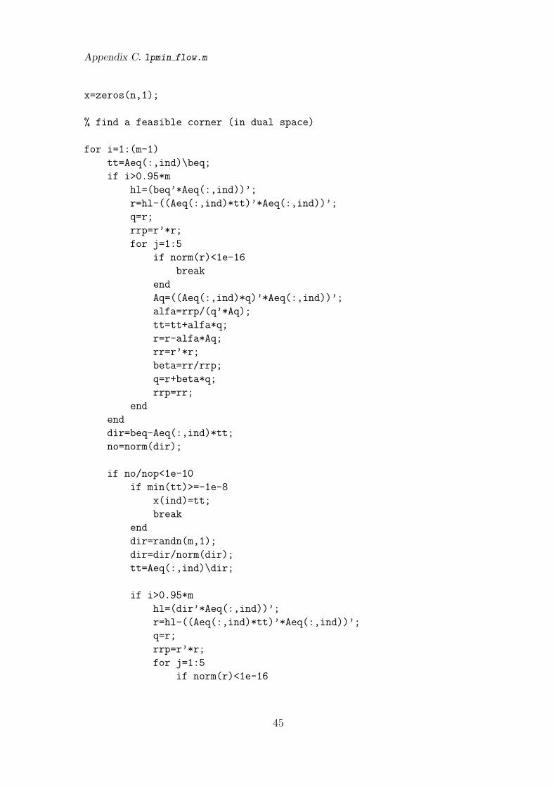
Appendix C. lpmin flow.m
x=zeros(n,1);
% find a feasible corner (in dual space)
for i=1:(m-1)
tt=Aeq(:,ind)\beq;
if i>0.95*m
hl=(beq’*Aeq(:,ind))’;
r=hl-((Aeq(:,ind)*tt)’*Aeq(:,ind))’;
q=r;
rrp=r’*r;
for j=1:5
if norm(r)<1e-16
break
end
Aq=((Aeq(:,ind)*q)’*Aeq(:,ind))’;
alfa=rrp/(q’*Aq);
tt=tt+alfa*q;
r=r-alfa*Aq;
rr=r’*r;
beta=rr/rrp;
q=r+beta*q;
rrp=rr;
end
end
dir=beq-Aeq(:,ind)*tt;
no=norm(dir);
if no/nop<1e-10
if min(tt)>=-1e-8
x(ind)=tt;
break
end
dir=randn(m,1);
dir=dir/norm(dir);
tt=Aeq(:,ind)\dir;
if i>0.95*m
hl=(dir’*Aeq(:,ind))’;
r=hl-((Aeq(:,ind)*tt)’*Aeq(:,ind))’;
q=r;
rrp=r’*r;
for j=1:5
if norm(r)<1e-16
45

Appendix C. lpmin flow.m
break
end
Aq=((Aeq(:,ind)*q)’*Aeq(:,ind))’;
alfa=rrp/(q’*Aq);
tt=tt+alfa*q;
r=r-alfa*Aq;
rr=r’*r;
beta=rr/rrp;
q=r+beta*q;
rrp=rr;
end
end
dir=dir-Aeq(:,ind)*tt;
no=norm(dir);
if no/nop<1e-9
break
end
diA=dir’*Aeq;
tvec=c_Ay./diA;
bol=not(ind);
[t,indind]=min(abs(tvec(bol)));
else
diA=dir’*Aeq;
tvec=c_Ay./diA;
bol=and(diA>0,not(ind));
[t,indind]=min(tvec(bol));
end
nop=no;
if length(t)>0
y=y+t*dir;
c_Ay=c_Ay-t*diA;
else
error(’Dual unbounded, primal infeasible’);
end
indp=ind;
ind=c_Ay<1e-15;
ind(indp)=1;
indvec=numind(bol);
ind(indvec(indind))=1;
end
% do simplex phase II (in dual space)
46

Appendix C. lpmin flow.m
if max(x)==0
for i=1:3*m
su=sum(ind);
if su==m
tt=Aeq(:,ind)\beq;
[ttmi,k]=min(tt);
if ttmi>-1e-13;
break
elseif ttmi==-Inf
hl=(beq’*Aeq(:,ind))’;
r=hl-((Aeq(:,ind)*tt)’*Aeq(:,ind))’;
q=r;
rrp=r’*r;
for j=1:5
if norm(r)<1e-16
break
end
Aq=((Aeq(:,ind)*q)’*Aeq(:,ind))’;
alfa=rrp/(q’*Aq);
tt=tt+alfa*q;
r=r-alfa*Aq;
rr=r’*r;
beta=rr/rrp;
q=r+beta*q;
rrp=rr;
end
dir=beq-Aeq(:,ind)*tt;
else
ek=zeros(m,1);
ek(k)=-1;
dir=Aeq(:,ind)’\ek;
dir=dir/norm(dir);
end
if dir’*beq<0
break
end
diA=dir’*Aeq;
tvec=c_Ay./diA;
t=min(tvec(and(diA>0,not(ind))));
if length(t)>0
y=y+t*dir;
c_Ay=c_Ay-t*diA;
47

Appendix C. lpmin flow.m
indp=ind;
cusu=cumsum(ind);
indred=find(cusu==k);
indp(indred(1))=0;
ind=c_Ay<1e-10;
ind(indp)=1;
else
error(’Dual unbounded, primal infeasible’);
end
elseif su>m
indp=ind;
ind1=randperm(su);
ind2=logical(zeros(su,1));
ind2(ind1(1:m))=1;
ind(ind)=ind2;
indp(indp)=not(ind2);
c_Ay(indp)=c_Ay(indp)+(min(norm(t*dir),1)*1e-2)*colnorm(indp);
else
ind=misor(c_Ay./colnorm,m);
end
end
end
% Find x
x(ind)=Aeq(:,ind)\beq;
function [ind,mii,maa]=misor(vec,p)
% index with the p smallest values
ind=logical(zeros(size(vec)));
[so,ind2]=sort(vec);
ind(ind2(1:p))=1;
maa=max(vec(ind));
mii=min(vec(ind));
48
References
[1] Ove Edlund. Solution of linear programming and non-linear regression prob-lems using linear M-estimation methods. Phd thesis, Lulea University of Tech-nology, http://epubl.luth.se/1402-1544/1999/17/, 1999. ISSN:1402-1544 ; 1999:17.
[2] George B Dantzig. Linear programming and extensions. 1968. Princeton, N.J. : Princeton Univ. Press, 1963. ISBN 0-691-08000-3.
[3] Gondzio J. and R. Kouwenberg. High performance computing for assetliability management. Technical report, Department of Mathematics &Statistics, The University of Edinburgh and Econometric Institute, ErasmusUniversity Rotterdam, http://www.maths.ed.ac.uk/~gondzio/software/wrecord.ps, 1999.
[4] H. Paul Williams. Model building in mathematical programming. 1999.Chichester : Wiley. ISBN 0-471-99788-9.
[5] Hillier, Frederick S and Lieberman, Gerald. Introduction to operations re-search. 2005. Boston : McGraw-Hill. ISBN 0-07-123828-X.
[6] Ciriani, Tito A and Leachman, Robert C. Optimization in industry : mathe-matical programming and modelling techniques in practice. 1993. Chichester; Wiley. ISBN 0-471-93492-5.
[7] Jan Lundgren, Mikael Ronnqvist, and Peter Varbrand. Introduction to op-erations research. 2003. Lund : Studentlitteratur. ISBN 91-44-03104-1.
[8] Athanasios Migdalas. Mathematical programming techniques for analysisand design of communication and transportation networks. 1988. Linkoping: Univ. ISBN 91-7870-302-6.
[9] David G Luenberger. Linear and nonlinear programming. 1984. Reading,Mass. : Addison-Wesley. ISBN 0-201-15794-2.
[10] Per Bergstrom. En algoritm for linjara optimeringsproblem. D-level thesis,Lulea University of Technology, http://epubl.ltu.se/1402-1552/2005/
04/, 2005.
[11] Gondzio J. and T. Terlaky. A computational view of interior point methodsfor linear programming. Technical report, Logilab, HEC Geneva, Section ofManagement Studies, University of Geneva,Faculty of Technical Mathematicsand Informatics, Delft University of Technology, http://www.maths.ed.ac.uk/~gondzio/software/oxford.ps, 1994.
49

[12] Andersen E.D., J. Gondzio, C. Meszaros, and X. Xu. Implementation ofinterior point methods for large scale linear programming. Technical report,Logilab, HEC Geneva, Section of Management Studies, University of Geneva,http://www.maths.ed.ac.uk/~gondzio/software/kluwer.ps, 1996.
50


