Solute tranport in periodical heterogeneous porous

media: importance of observation scale and

experimental sampling

Samer Majdalani, Jean-Philippe Chazarin, Carole Delenne, Vincent Guinot

To cite this version:

Samer Majdalani, Jean-Philippe Chazarin, Carole Delenne, Vincent Guinot. Solute tranportin periodical heterogeneous porous media: importance of observation scale and experimentalsampling. Journal of Hydrology, Elsevier, 2015, 520, pp.52-60. .

HAL Id: hal-01101494

https://hal.archives-ouvertes.fr/hal-01101494

Submitted on 9 Jan 2015

HAL is a multi-disciplinary open accessarchive for the deposit and dissemination of sci-entific research documents, whether they are pub-lished or not. The documents may come fromteaching and research institutions in France orabroad, or from public or private research centers.

L’archive ouverte pluridisciplinaire HAL, estdestinee au depot et a la diffusion de documentsscientifiques de niveau recherche, publies ou non,emanant des etablissements d’enseignement et derecherche francais ou etrangers, des laboratoirespublics ou prives.

1

Solute transport in periodical heterogeneous porous media: Importance 1

of observation scale and experimental sampling  2

3 S. Majdalani (1), J.P. Chazarin (2) , C. Delenne (1), V. Guinot (1, 3). 4 5 6 (1) Université Montpellier 2 Polytech Montpellier/HSM, CC 057, Place Eugène Bataillon, 34095 7 Montpellier Cedex 5, France 8 (2) Institut de Recherche pour le Développement (IRD)/ HSM, CC 057, Place Eugène Bataillon, 9 34095 montpellier Cedex 5, France 10 (3) Inria, Team LEMon 11 12 Corresponding Author: Samer Majdalani 13 Tel: +33 4 67 14 90 59 14 Fax : +33 4 67 14 47 74 15

Email: samer.majdalani@msem.univ-montp2.fr 16 17 18 19 20 21 Acepted for publication in Journal of Hydrology, 520, 52-60, 2015 22

23

24

2

Abstract 1

This paper focuses on the effects of the observation scale and sampling on the dispersion of tracers in 2 periodical heterogeneous porous media. A Model Heterogeneous Porous Medium (MHPM) with a 3 high degree of heterogeneity was built. It consists of a preferential flow path surrounded by glass 4 beads. 44 tracer experiments were carried out on several series of periodic MHPM to investigate the 5 effect of the observation scale on solute dispersion. Each series was replicated several times, allowing 6 for a statistical description of the unit transfer function of the MHPM. No significant trend was found 7 for the dispersion coefficient as a function of the size of the MHPM. However, given the variability of 8 the breakthrough curves from one experiment replicate to another, under-sampling might easily lead to 9 conclude that the dispersion coefficient is variable with distance. Depending on the samples used, it 10 would be as easy to (wrongly) detect an increasing trend as to detect a decreasing one. A confidence 11 interval analysis of the experimental breakthrough curves in the Laplace space shows that (i) there 12 exists a model with scale independent parameters that can describe the experimental breakthrough 13 curves within the limits of experimental uncertainty, (ii) this model is not the Advection-Dispersion 14 (AD) model, (iii) the modelling error of the AD model decreases with the number of periods, (iv) the 15 size of the Reference Elementary Volume for the dispersion coefficient is between 10 and 20 periods. 16 The effects of sampling prove to override those of scaling. This, with the invalidity of the AD model, 17 leads to question attempts to calibrate and/or identify trends in the dispersion coefficient at 18 intermediate scales from a limited number of experiment replicates. 19

Keywords 20

Dispersion modelling 21 Intermediate Scale Experiment 22 Heterogeneous media 23

1. Introduction 24

Understanding solute transport in porous media is important to predict the fate of contaminants in 25 natural soils. Natural soils are highly heterogeneous and implicate various transport mechanisms. 26 Tracer experiments on laboratory soil columns made a big contribution to identify these mechanisms. 27 The most widespread transport model for inert solute is the Advection-Dispersion (AD) model. Fitting 28 this model against real-world tracer tests has been reported to induce an increase in the dispersion 29 coefficient with the travelled distance (see e.g. Dagan, 1989; Gelhar et al., 1992; Zhou and Selim, 30 2003). The variability of the dispersion coefficient with distance has motivated a strong interest for 31 alternative models. Recently, laboratory tracer experiments have been used as a benchmarking basis to 32 test the respective accuracy of a variety of normal and anomalous transport models (see e.g. the review 33 in Gao et al., 2009). It has also been suggested by some authors that the dispersion coefficient in 34 mobile-immobile models should be made exponentially dependent on distance in order to accurately 35 reproduce experimental breakthrough curves in laboratory column experiments (Gao et al., 2010). 36 37 A number of laboratory tracer experiments in porous media are available from the literature (Silliman 38 et al., 1998). Laboratory experiments on heterogeneous porous media are very few in comparison to 39 those done on homogeneous porous media. One cause might be the practical difficulty to conceive and 40 construct heterogeneous porous media. 41 42 Silliman and Simpson (1987) used fine sand inclusions (small cubes) with coarse sand surrounding. 43 They found a change in the shape of the breakthrough curve at each of five measurement sections, and 44 inferred a continuous increase in dispersivity with distance. Saiers et al. (1994) used a coarse sand 45 inclusion (tubule) with finer sand surrounding. The inclusion constituted a preferential flow path and 46 contributed to more than 60% of the mass balance. The breakthrough curves exhibited multiple 47 inflection points that cannot be accounted for by the classical Advection Dispersion (AD) model. In 48 comparison to other studies, the work of Saiers et al. (1994) is distinguished by the high degree of 49 heterogeneity of the porous media. This fact is reflected in the shape of the breakthrough curves. Much 50

3

more than a mere tailing effect, the breakthrough curves exhibited a clear two-step shape. Li et al. 1 (1994) used coarse inclusions (polyethylene porous cylinders) with finer sand surrounding. The 2 resulting breakthrough curves exhibited asymmetry. Huang et al. (1995) used a 12.5 m long column 3 with a wide range of soil materials. Their breakthrough curves exhibited irregular and nonsigmoidal 4 distributions and were in most cases poorly described by the AD model. 5 6 Sternberg et al. (1996) and Irwin et al. (1996) were the first to use a periodical heterogeneous porous 7 media, where the heterogeneity consisted of a succession of several glass bead sets tested in several 8 serial orders. The breakthrough curves were used to infer the variation of the dispersion coefficient 9 with distance. Unfortunately, the breakthrough curves are not shown in the publications and no 10 estimate is provided for the goodness-of-fit of the AD model. It is thus impossible to determine 11 whether fitting the coefficients of the AD model was meaningful. However, both studies present the 12 results of dispersion estimations. Sternberg et al. (1996) found that dispersion does not necessarily 13 increase with scale, but that it can increase and decrease depending on the particular arrangement of 14 properties in the medium. They deduced that the system length was unimportant in observing the scale 15 effect. Conversely, in the study of Irwin et al. (1996), dispersion appeared to be scale dependent up to 16 a certain travel distance. But, quoting the authors’ own words, "because of the scatter in the data, it 17 could be argued that the apparent increase in longitudinal dispersion is simply a result of the variation 18 in the data". This raises the issue of sampling effects. 19 20 Greiner et al. (1997) used aggregates of lower permeability in a surrounding of higher permeability. 21 Niehren and Kinzelbach (1998) used cylindrical cellpore filters (less permeable) in a quartzsand 22 surrounding (more permeable). Tran Ngoc et al. (2011) used spherical clay inclusions (micro porosity) 23 surrounded by sand (macro porosity). Danquigny et al. (2004) performed tracer tests on two kinds of 24 heterogeneous porous material: a channel structured medium (5.6m×1m×1m), with channels crossing 25 the whole tank, and a statistically correlated random structure. They found that the breakthrough 26 curves of the statistically correlated random structure could be fitted with the AD model (at least for 27 long distances), but that the fit is quite poor for channel structured model due to the non-Gaussian 28 distribution of the concentration. 29 Zin et al. (2004) designed an artificial porous medium with several conductivity contrasts, using low 30 conductivity inclusions (small beads) surrounded by a high conductivity matrix (large beads). They 31 found that the breakthrough curves of the low-contrast medium showed no tailing, while those of high-32 contrast medium showed tailing. Golfier et al. (2011) used fine sand inclusions (lenses) with coarse 33 sand surrounding. Their breakthrough curves showed asymmetry. The low degree of heterogeneity in 34 the studies of Sternberg et al. (1996) and Irwin et al. (1996) might have led to some contradictory 35 conclusions concerning the dispersion scale dependence. As to the study of Saiers et al. (1994), the 36 authors were not mainly interested in the problematic of dispersion scale dependence, but rather in 37 colloidal mobilization and transport in a structured porous media. 38 39 In the light of the abovementioned studies, it appears that studying the effect of heterogeneity on 40 solute transport requires two conditions: (i) a high degree of heterogeneity of the porous media (as the 41 experimental model of Saiers et al. (1994)), and (ii) a periodical heterogeneous porous media (as the 42 experimental protocol of Sternberg et al. (1996) and Irwin et al. (1996)). The first condition guarantees 43 that the effects of material heterogeneity are clearly visible, while the second allows the influence of 44 scale effects to be assessed. This also allows for a better quality of the experimental data, with easily 45 replicable experiments yielding reliable statistics. 46 47 In this study, we conceived a Model Heterogeneous Porous Medium (MHPM) with a high degree of 48 heterogeneity. The purpose is to (i) enrich the experimental database of laboratory tracer tests with 49 high quality data, (ii) answer the following six questions. 50 (Q1) Can a scaling trend be observed for the dispersion coefficient in this highly heterogeneous 51

MHPM? 52 (Q2) If this is not the case, can the variations of the dispersion with the observation scale be 53

attributed to experimental artefacts such as sampling effects? 54

4

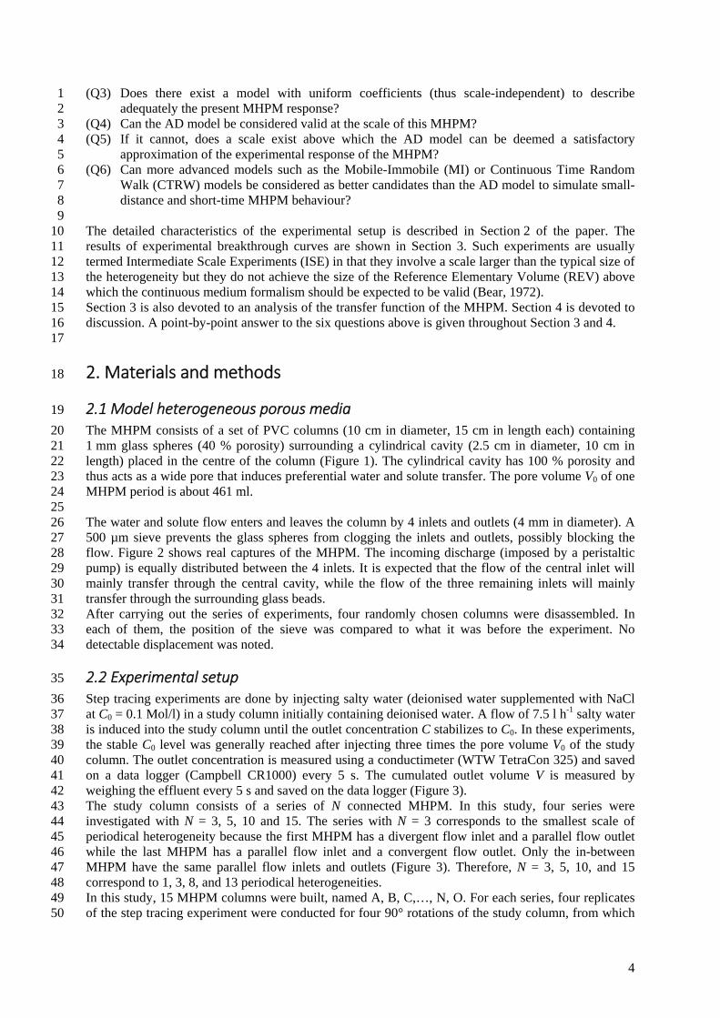
(Q3) Does there exist a model with uniform coefficients (thus scale-independent) to describe 1 adequately the present MHPM response? 2

(Q4) Can the AD model be considered valid at the scale of this MHPM? 3 (Q5) If it cannot, does a scale exist above which the AD model can be deemed a satisfactory 4

approximation of the experimental response of the MHPM? 5 (Q6) Can more advanced models such as the Mobile-Immobile (MI) or Continuous Time Random 6

Walk (CTRW) models be considered as better candidates than the AD model to simulate small-7 distance and short-time MHPM behaviour? 8

9 The detailed characteristics of the experimental setup is described in Section 2 of the paper. The 10 results of experimental breakthrough curves are shown in Section 3. Such experiments are usually 11 termed Intermediate Scale Experiments (ISE) in that they involve a scale larger than the typical size of 12 the heterogeneity but they do not achieve the size of the Reference Elementary Volume (REV) above 13 which the continuous medium formalism should be expected to be valid (Bear, 1972). 14 Section 3 is also devoted to an analysis of the transfer function of the MHPM. Section 4 is devoted to 15 discussion. A point-by-point answer to the six questions above is given throughout Section 3 and 4. 16 17

2. Materials and methods 18

2.1 Model heterogeneous porous media 19

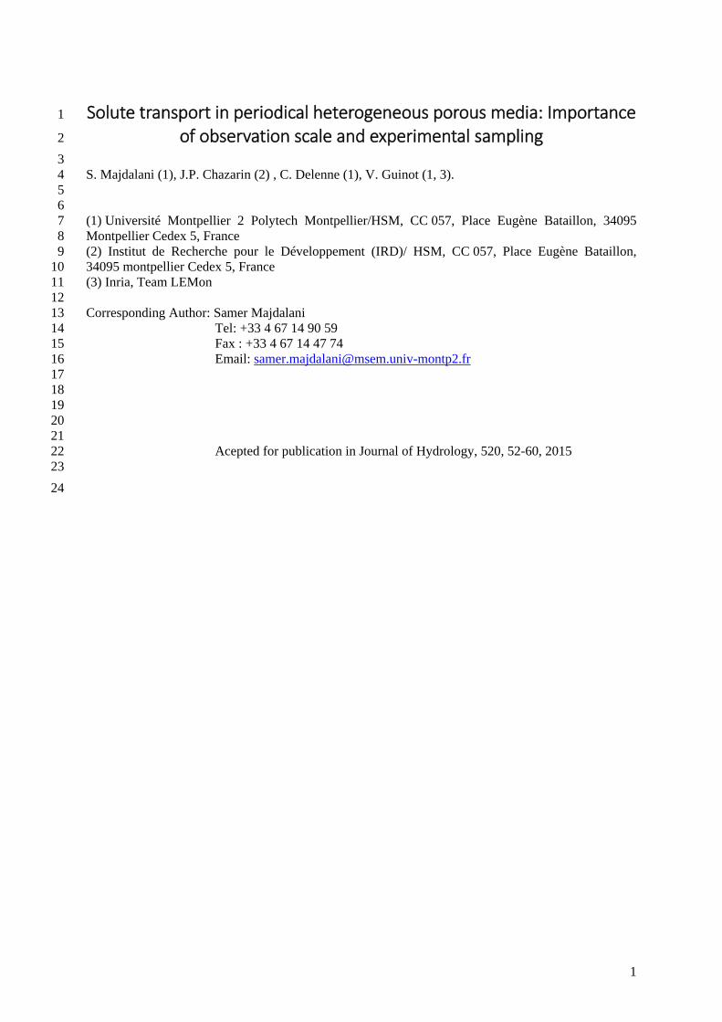
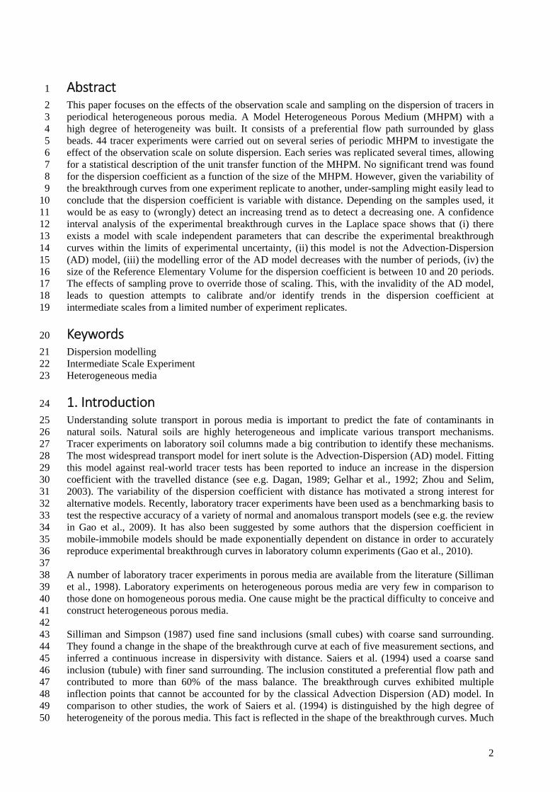
The MHPM consists of a set of PVC columns (10 cm in diameter, 15 cm in length each) containing 20 1 mm glass spheres (40 % porosity) surrounding a cylindrical cavity (2.5 cm in diameter, 10 cm in 21 length) placed in the centre of the column (Figure 1). The cylindrical cavity has 100 % porosity and 22 thus acts as a wide pore that induces preferential water and solute transfer. The pore volume V0 of one 23 MHPM period is about 461 ml. 24 25 The water and solute flow enters and leaves the column by 4 inlets and outlets (4 mm in diameter). A 26 500 µm sieve prevents the glass spheres from clogging the inlets and outlets, possibly blocking the 27 flow. Figure 2 shows real captures of the MHPM. The incoming discharge (imposed by a peristaltic 28 pump) is equally distributed between the 4 inlets. It is expected that the flow of the central inlet will 29 mainly transfer through the central cavity, while the flow of the three remaining inlets will mainly 30 transfer through the surrounding glass beads. 31 After carrying out the series of experiments, four randomly chosen columns were disassembled. In 32 each of them, the position of the sieve was compared to what it was before the experiment. No 33 detectable displacement was noted. 34

2.2 Experimental setup 35

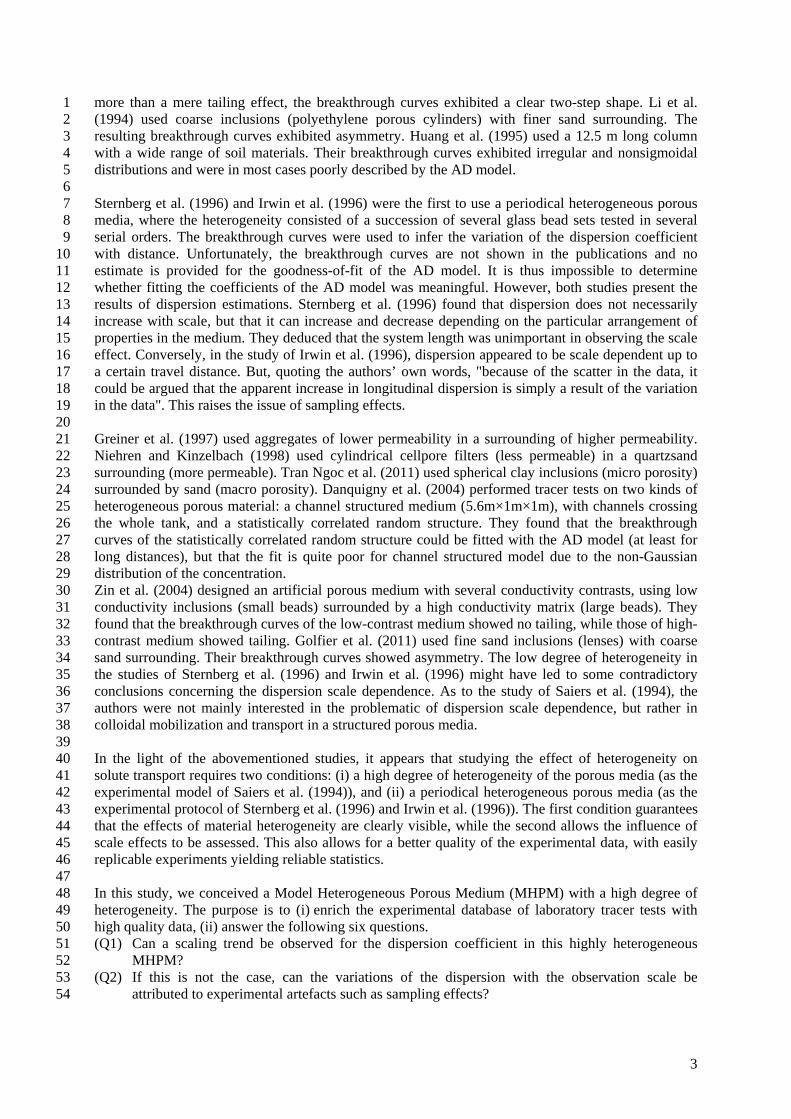
Step tracing experiments are done by injecting salty water (deionised water supplemented with NaCl 36 at C0 = 0.1 Mol/l) in a study column initially containing deionised water. A flow of 7.5 l h-1 salty water 37 is induced into the study column until the outlet concentration C stabilizes to C0. In these experiments, 38 the stable C0 level was generally reached after injecting three times the pore volume V0 of the study 39 column. The outlet concentration is measured using a conductimeter (WTW TetraCon 325) and saved 40 on a data logger (Campbell CR1000) every 5 s. The cumulated outlet volume V is measured by 41 weighing the effluent every 5 s and saved on the data logger (Figure 3). 42 The study column consists of a series of N connected MHPM. In this study, four series were 43 investigated with N = 3, 5, 10 and 15. The series with N = 3 corresponds to the smallest scale of 44 periodical heterogeneity because the first MHPM has a divergent flow inlet and a parallel flow outlet 45 while the last MHPM has a parallel flow inlet and a convergent flow outlet. Only the in-between 46 MHPM have the same parallel flow inlets and outlets (Figure 3). Therefore, N = 3, 5, 10, and 15 47 correspond to 1, 3, 8, and 13 periodical heterogeneities. 48 In this study, 15 MHPM columns were built, named A, B, C,…, N, O. For each series, four replicates 49 of the step tracing experiment were conducted for four 90° rotations of the study column, from which 50

5

a mean breakthrough curve was deduced. The purpose of the 90° rotation is to eliminate biases 1 resulting from a possible interaction between density-driven effects and the 120° spacing between the 2 column inlets and outlets. The various column combinations used for the various experiments are 3 summarized in Table 1. 4 5 N V0 (ml) L (m) Column groups Total replicates 3 1383 0.45 ABC, FGH, DEJ, KLM, INO 20 5 2305 0.75 ABCDE, FGHIJ, KLMNO 12 10 4610 1.50 A–J, F–O 8 15 6915 2.25 A–O 4

Table 1. Experimental configurations. L is the total length of the porous media. 6

3. Experimental results 7

3.1 Experimental  breakthrough curve 8

For each value of N, four experimental signals are computed: the average breakthrough concentration 9

)(tC , its standard deviation C , the minimum and maximum breakthrough concentrations, defined as 10

)(max)(),(min)(

,)()(1

1,)(

1)(

maxmin

1

22

1

tCtCtCtC

tCtCR

tCR

tC

ii

ii

R

iiC

R

ii

(1) 11

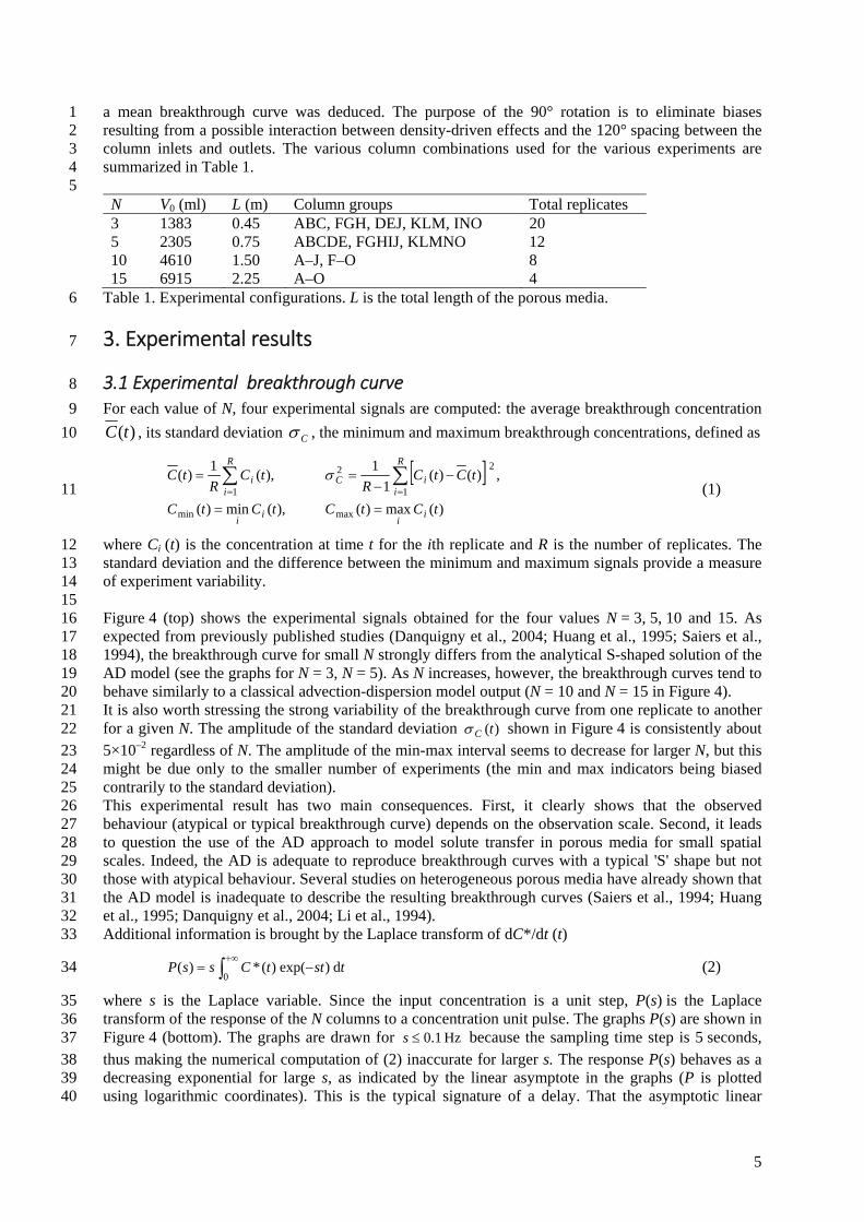
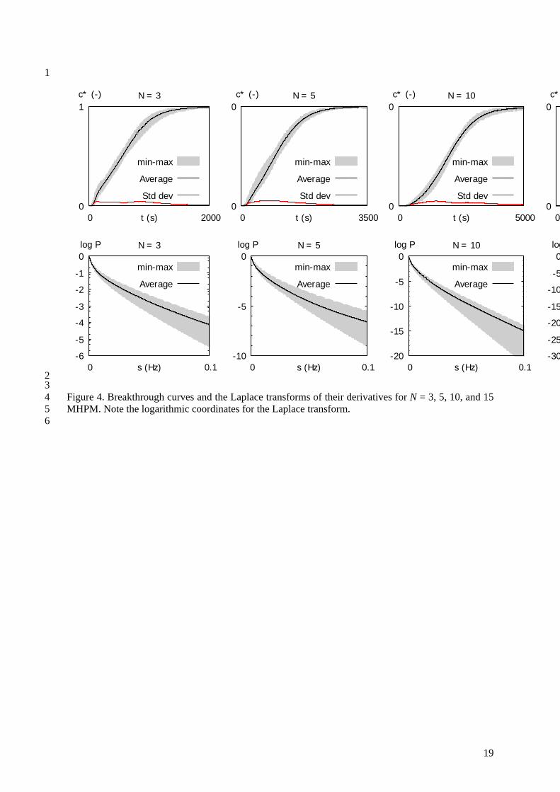
where Ci (t) is the concentration at time t for the ith replicate and R is the number of replicates. The 12 standard deviation and the difference between the minimum and maximum signals provide a measure 13 of experiment variability. 14 15 Figure 4 (top) shows the experimental signals obtained for the four values N = 3, 5, 10 and 15. As 16 expected from previously published studies (Danquigny et al., 2004; Huang et al., 1995; Saiers et al., 17 1994), the breakthrough curve for small N strongly differs from the analytical S-shaped solution of the 18 AD model (see the graphs for N = 3, N = 5). As N increases, however, the breakthrough curves tend to 19 behave similarly to a classical advection-dispersion model output (N = 10 and N = 15 in Figure 4). 20 It is also worth stressing the strong variability of the breakthrough curve from one replicate to another 21 for a given N. The amplitude of the standard deviation )(tC shown in Figure 4 is consistently about 22 5×10–2 regardless of N. The amplitude of the min-max interval seems to decrease for larger N, but this 23 might be due only to the smaller number of experiments (the min and max indicators being biased 24 contrarily to the standard deviation). 25 This experimental result has two main consequences. First, it clearly shows that the observed 26 behaviour (atypical or typical breakthrough curve) depends on the observation scale. Second, it leads 27 to question the use of the AD approach to model solute transfer in porous media for small spatial 28 scales. Indeed, the AD is adequate to reproduce breakthrough curves with a typical 'S' shape but not 29 those with atypical behaviour. Several studies on heterogeneous porous media have already shown that 30 the AD model is inadequate to describe the resulting breakthrough curves (Saiers et al., 1994; Huang 31 et al., 1995; Danquigny et al., 2004; Li et al., 1994). 32 Additional information is brought by the Laplace transform of dC*/dt (t) 33

0

d)exp()(*)( tsttCssP (2) 34

where s is the Laplace variable. Since the input concentration is a unit step, P(s) is the Laplace 35 transform of the response of the N columns to a concentration unit pulse. The graphs P(s) are shown in 36 Figure 4 (bottom). The graphs are drawn for Hz1.0s because the sampling time step is 5 seconds, 37 thus making the numerical computation of (2) inaccurate for larger s. The response P(s) behaves as a 38 decreasing exponential for large s, as indicated by the linear asymptote in the graphs (P is plotted 39 using logarithmic coordinates). This is the typical signature of a delay. That the asymptotic linear 40

6

behaviour is reached for smaller s as N increases indicates that advection phenomena become 1 predominant as N increases, a well-known feature of the advection-dispersion model for increasing 2 Peclet number values. This, however, is not sufficient to validate the AD model, an issue that is 3 addressed in Section 4.1. 4

3.2 Scaling trend for the dispersion coefficient 5

Questions (Q1) and (Q2) are answered assuming that the AD model is valid, with governing equations 6

02

2

x

CD

x

Cu

t

C (3a) 7

LxxC ,00)0,( (3b) 8

where D is the dispersion coefficient, and u the flow velocity. Analytical solutions are available for an 9 upstream boundary condition in the form of a step flux function (Ogata and Banks 1961) 10

22erfcexp

2erfc),(00),0( 0

2/12/1

C

Dt

utx

D

ux

Dt

utxtxCttC

(4) 11

The unit response to a Dirac flux pulse is obtained as the derivative of (4) with respect to time 12

Dt

utxutx

Dt

utxutx

Dt

CtxCtCtC

4

)(exp

4

)(exp

)(4),()(),0(

2

2

2/32/10

0

(5) 13

The Laplace transform of the solution (5) can also be obtained by solving equation (3) in the space-14 Laplace domain: 15

2/1

2

41,

2

1exp

1

2),(ˆ

su

DF

F

D

ux

FsxC (6) 16

The experimental dispersion coefficient D is computed using a formula derived from the analytical 17 solution of the advection-dispersion equation (Bear 1972): 18

50

22

50

40602

50

4060 22t

L

t

ttLu

t

ttD

(7) 19

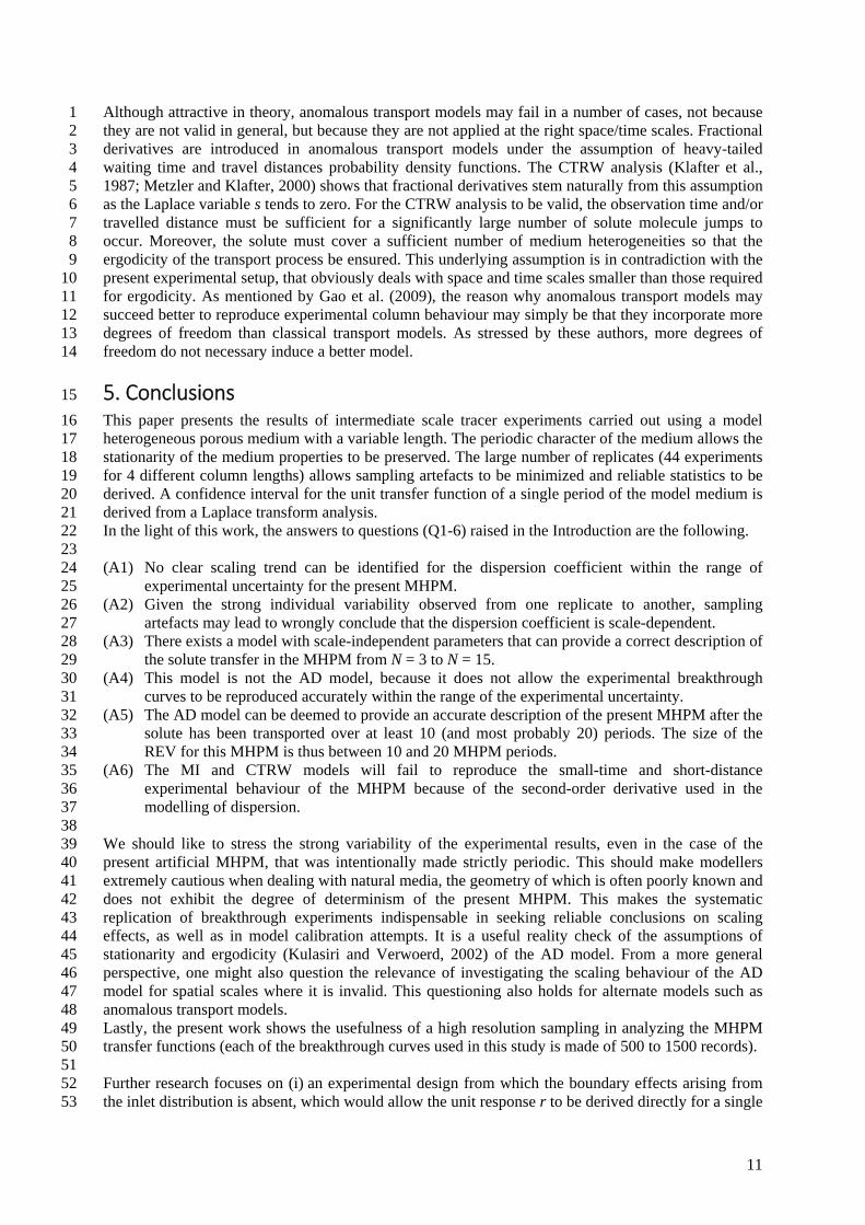
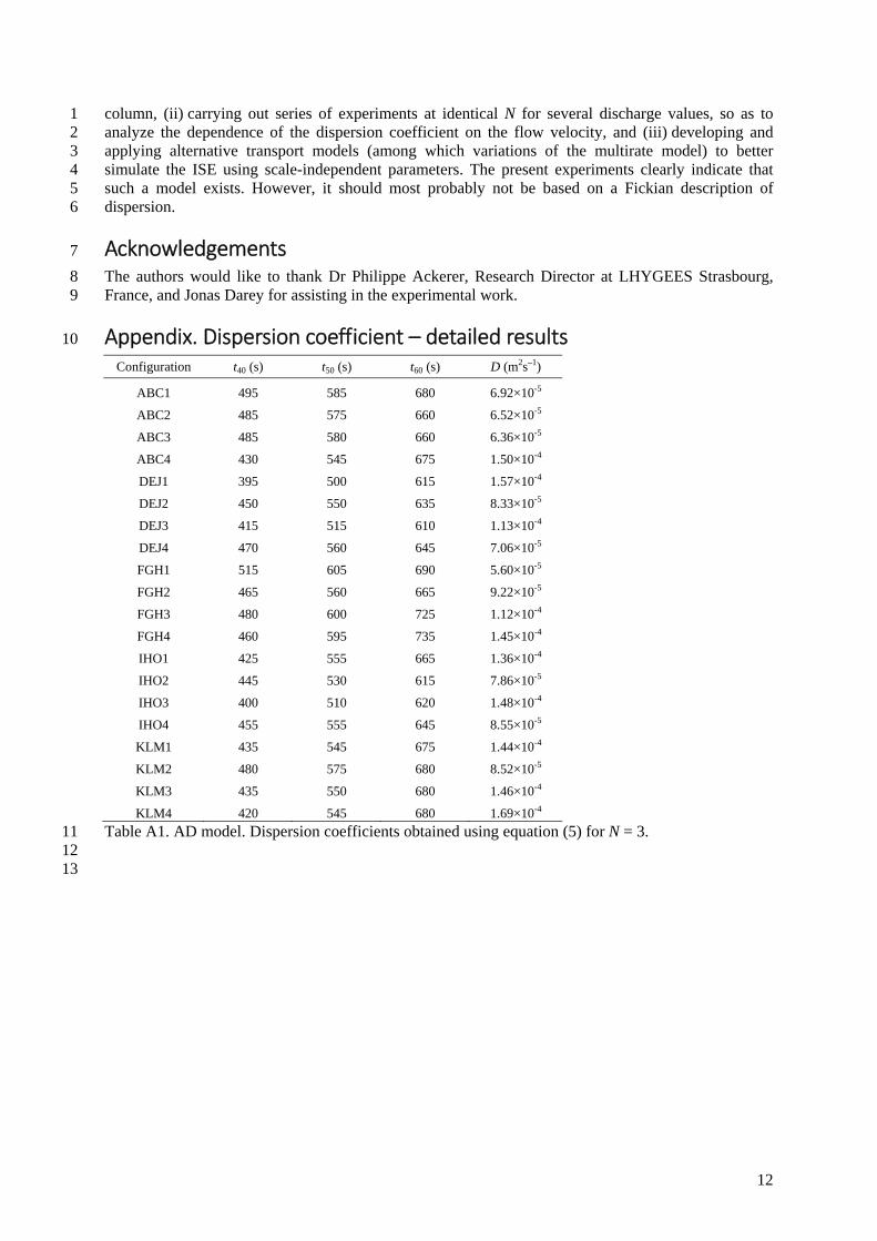
used by e.g. Irwin et al. (1996) and Sternberg et al. (1996). 20 Equation (5) was applied to the experimental configurations shown in Table 1. The detailed results are 21 given in the Appendix (Tables A1 to A4), only statistics are presented here. For each value of N, the 22 average, standard deviation, minimum and maximum of D obtained from the various possible 23 configurations are provided in Table 2. Several remarks can be made at this stage. 24 Firstly, the variations in the average D with L are smaller than the standard deviation of D for any 25 given L. Since the individual variations between the replicates for a given N override by far any visible 26 trend, it can be concluded that no significant trend of distance-dependent dispersion D(L) is detected 27 given the experimental uncertainty. 28 Secondly, given the range of variations between the minimum and maximum values, it is possible to 29 find a sequence among all the experimental values in Tables A1-4 such that an increasing trend D(L) 30 is detected. An example of such a sequence is (ABC1, ABCDE2, A–J4, A–O4). But it would be just as 31 easy to detect a decreasing trend D(L) by choosing the values in Tables A1–4 appropriately, for 32 instance the sequence (KLM4, FGHIJ3, K–O2, A–O3). Such trends, however, would only be sampling 33 artefacts. 34 35 It can be concluded as an answer to question (Q1) that, in the limit of experimental uncertainty, no 36 significant scaling trend can be identified for the dispersion coefficient in the present MHPM. As an 37

7

answer to question (Q2), sampling artefacts may easily lead to the conclusion that the dispersion 1 coefficient is subjected to a scaling trend in this MHPM. It is stressed that only the systematic 2 replication of the tracer experiments and a high-resolution sampling allows this question to be 3 answered with a satisfactory degree of confidence. 4 5

L (m) N D (m2s–1) average D (m2s–1) standard

deviation D (m2s–1) minimum D (m2s–1) maximum

0.45 3 1.08×10–4 3.65×10–5 5.60×10–5 1.69×10–4

0.75 5 1.36×10–4 6.37×10–5 7.40×10–5 3.29×10–4

1.50 10 1.18×10–4 3.38×10–5 6.58×10–5 1.81×10–4

2.25 15 1.18×10–4 3.00×10–5 8.43×10–5 1.67×10–4

Table 2. AD model. Dispersion coefficients obtained using equation (7). See the detailed results in the 6 Appendix. 7

3.3 Unit transfer function 8

The purpose of the present subsection is to answer question (Q3). Since the various replicates Ci(t) all 9 give different time series for a given number N of columns, the unit transfer function is different for 10 each replicate. The proposed approach consists in determining the envelope of all possible C(t) signals 11 for a Dirac input. It is obvious from Definition (1) that neither the lower bound Cmin nor the upper 12 bound Cmax of this envelope do correspond to a single replicate signal Ci(t), the purpose being only to 13 determine the range of possible variations of C(t) for each time t. 14 For this, it is necessary to estimate the unit transfer function of a single MHPM period. Denote by PN,i 15 the Laplace transform of the ith replicate for a number N of columns. A minimum-maximum 16 confidence interval is defined for P with the following lower and upper bounds: 17

iNRi

NiNRi

N PPPP ,,,1

max,,,,1

min, max,min

(8) 18

where N denotes the number of columns used in the experiment and i denotes the replicate. This 19 allows a confidence interval to be defined for the unit Laplace transform of a single MPMH period. 20 Let r be the Laplace transform of a single MHPM period for a Dirac concentration input. The lower 21 and upper bounds defined in (8) yield a confidence interval ),(),,( maxmin NMrNMr for r. Indeed, the 22 convolution property of the Laplace transform leads to 23

NMNMNMrrNMr ,,),(),( maxmin (9a) 24

NMP

PNMr

P

PNMr

MN

M

NMN

M

N

,,,,

1

min,

max,max

1

max,

min,min (9b) 25

If a unit transfer function with scale-independent parameters exists, all the confidence intervals 26 ),(),,( maxmin NMrNMr derived for all possible combinations (M, N) should overlap. Denoting 27 respectively by r1 and r2 the lower and upper bounds of the intersection of all the confidence intervals, 28 one has by definition 29

NMrrNMrrNMNM

,min,,max max,

2min,

1 (10) 30

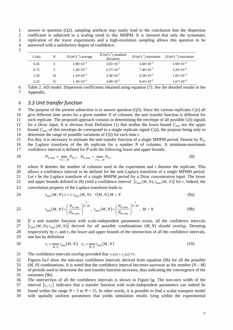
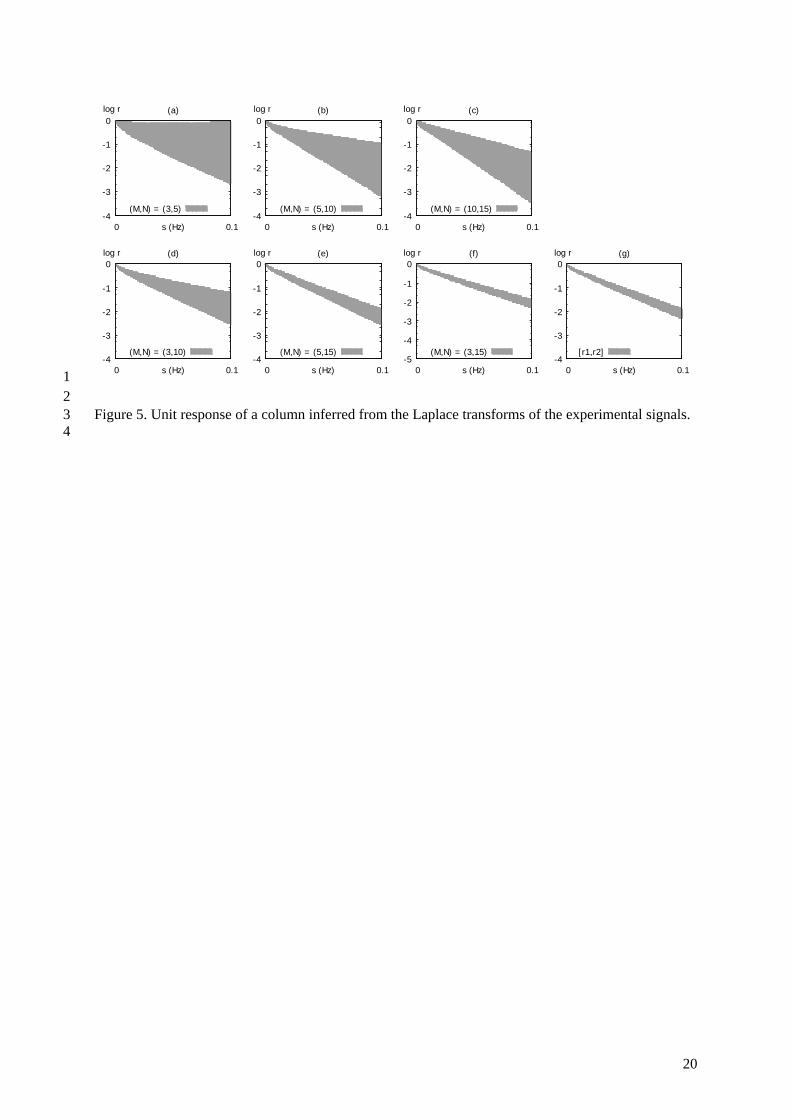
The confidence intervals overlap provided that ssrsr )()( 21 . 31 Figures 5a-f show the min-max confidence intervals derived from equation (9b) for all the possible 32 (M, N) combinations. It is noted that the confidence interval becomes narrower as the number (N – M) 33 of periods used to determine the unit transfer function increases, thus indicating the convergence of the 34 estimates (9b). 35 The intersection of all the confidence intervals is shown in Figure 5g. The non-zero width of the 36 interval 21 , rr indicates that a transfer function with scale-independent parameters can indeed be 37 found within the range N = 3 to N = 15. In other words, it is possible to find a scalar transport model 38 with spatially uniform parameters that yields simulation results lying within the experimental 39

8

uncertainty. This model, however, is not necessarily the classical AD model. This issue is explored in 1 the next section. 2

4. Discussion 3

4.1 Validity of the AD model 4

The purpose of the present section is to answer questions (Q4-5). If the AD model is valid at the scale 5 of N MHPM periods, then there exists a combination (D, u) such that 6

ssrsNlCsr NN )(),(ˆ)( 21 (11) 7

where l = 15 cm is the length of a single MHPM period. Clearly, this condition is not satisfied for 8 N = 1. Indeed, for large s, the analytical solution (6) behaves as 9

2/1

2/12/12/12/12/1 exp),(ˆ2

sD

Nl

sD

usNlCsD

uF (13) 10

a function with a horizontal asymptotic direction in semi-logarithmic coordinates, while r1(s) and r2(s) 11

take the form of straight lines for large s (see Figure 5g). Consequently, the function ),(ˆ sNlC does not 12

lie within the interval NN rr 21 , for all s and the AD model is invalid to some extent. This is illustrated 13

by Figure 6a, where the confidence interval NN rr 21 , and the function sNlC ,ˆ are plotted for N = 1. 14 The degree of accuracy of the AD model is assessed by computing the L2-norm of the difference 15 between the experimental transfer function and the theoretical one in the Laplace space: 16

2/1

0

22 d)(

1

Sss

SL (13a) 17

)(),(ˆif)(),(ˆ)(),(ˆ)(if0

)(),(ˆif)(),(ˆ

)(

22

21

11

srsNlCsrsNlC

srsNlCsr

srsNlCsrsNlC

sNN

NN

NN

(13b) 18

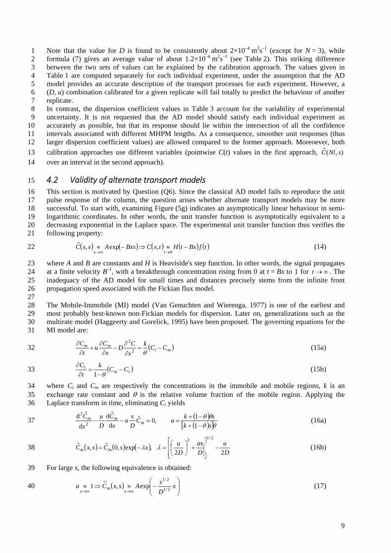
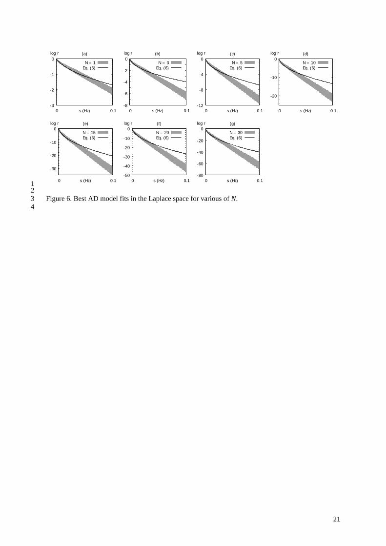
where S = 0.1 Hz is the upper bound of s. Eq. (13b) gives a zero error if the solution of the AD model 19 lies between r1 and r2 in the Laplace space, that is, if the AD solution falls within the range of the 20 experimental uncertainty. 21 Table 3 shows the combinations (D, u) that minimize the L2-norm (13a) for various values of N. 22 Figure 6a-g shows the corresponding plots in the Laplace space. The L2-norm for N = 1 is large, 23 indicating that the AD model provides a poor description of the transfer process at the scale of a single 24 column. However, the L2-norm decreases quickly with N, which is an indication that the AD model 25 gains worth with the number of MHPM periods. The driving mechanism for this is interesting to 26 notice. As shown by Figures 6a-g, the AD transfer function lies outside the confidence interval for 27 s > 3×10–2 Hz in all graphs. In other words, in terms of relative error, the AD model is equally 28 inaccurate for all values of N. However, the amplitude of the transfer function decreases quickly as N 29 increases. The absolute value of the error thus becomes smaller as N increases. 30 31

N D u L2 Figure 1 1.57×10–4 1.98×10–3 2.13×10–3 6a 3 2.85×10–4 1.18×10–3 1.27×10–4 6b 5 2.36×10–4 9.98×10–4 1.70×10–6 6c

10 2.24×10–4 7.97×10–4 1.75×10–10 6d 15 2.07×10–4 7.71×10–4 6.51×10–15 6e 20 2.07×10–4 7.71×10–4 2.045×10–18 6f 30 2.07×10–4 7.71×10–4 2.66×10–25 6g

Table 3. AD model. Optimal parameter set for the objective function (13a-b). 32 33

9

Note that the value for D is found to be consistently about 2×10–4 m2s–1 (except for N = 3), while 1 formula (7) gives an average value of about 1.2×10–4 m2s–1 (see Table 2). This striking difference 2 between the two sets of values can be explained by the calibration approach. The values given in 3 Table 1 are computed separately for each individual experiment, under the assumption that the AD 4 model provides an accurate description of the transport processes for each experiment. However, a 5 (D, u) combination calibrated for a given replicate will fail totally to predict the behaviour of another 6 replicate. 7 In contrast, the dispersion coefficient values in Table 3 account for the variability of experimental 8 uncertainty. It is not requested that the AD model should satisfy each individual experiment as 9 accurately as possible, but that its response should lie within the intersection of all the confidence 10 intervals associated with different MHPM lengths. As a consequence, smoother unit responses (thus 11 larger dispersion coefficient values) are allowed compared to the former approach. Moreoever, both 12

calibration approaches use different variables (pointwise C(t) values in the first approach, ),(ˆ sNlC 13 over an interval in the second approach). 14

4.2  Validity of alternate transport models 15

This section is motivated by Question (Q6). Since the classical AD model fails to reproduce the unit 16 pulse response of the column, the question arises whether alternate transport models may be more 17 successful. To start with, examining Figure (5g) indicates an asymptotically linear behaviour in semi-18 logarithmic coordinates. In other words, the unit transfer function is asymptotically equivalent to a 19 decreasing exponential in the Laplace space. The experimental unit transfer function thus verifies the 20 following property: 21

tfBxtHtxCBxsAsxCts

0

,exp,ˆ (14) 22

where A and B are constants and H is Heaviside's step function. In other words, the signal propagates 23 at a finite velocity B–1, with a breakthrough concentration rising from 0 at t = Bx to 1 for t . The 24 inadequacy of the AD model for small times and distances precisely stems from the infinite front 25 propagation speed associated with the Fickian flux model. 26 27 The Mobile-Immobile (MI) model (Van Genuchten and Wierenga, 1977) is one of the earliest and 28 most probably best-known non-Fickian models for dispersion. Later on, generalizations such as the 29 multirate model (Haggeerty and Gorelick, 1995) have been proposed. The governing equations for the 30 MI model are: 31

mimm CC

k

x

CD

x

Cu

t

C

2

2

(15a) 32

imi CC

k

t

C

1 (15b) 33

where Ci and Cm are respectively the concentrations in the immobile and mobile regions, k is an 34 exchange rate constant and is the relative volume fraction of the mobile region. Applying the 35 Laplace transform in time, eliminating Ci yields 36

sk

skaC

D

sa

x

C

D

u

x

Cm

mm

1

1,0ˆ

d

ˆd

d

ˆd2

2

(16a) 37

D

u

D

as

D

uxsCsxC mm 22

,exp,0ˆ,ˆ2/12

(16b) 38

For large s, the following equivalence is obtained: 39

x

D

sAsxCa

sm

s 2/1

2/1

exp,~

1 (17) 40

10

leading to a horizontal asymptotic direction in the semi-logarithmic plots of Figures 4 to 6. 1

Consequently, the ),(ˆ sxCm curve (16) cannot remain between the min-max bounds of the 2 experimental confidence interval for large s, thereby failing to account for the experimental MHPM 3 behaviour for small times. 4 5 The modelling community's attention has been drawn over the past years to anomalous transport 6 models (see e.g. Gao et al, 2009 for a review). Anomalous transport models use a non-Fickian model 7 for dispersion. The underlying assumption is that the characteristic time scale and/or the characteristic 8 length of the solute movement are infinite. Under such conditions, the assumption of Brownian 9 movement is no longer valid and long-term memory effects appear. The general form for anomalous 10 transport models is 11

1,1

10

10

,01

1

x

C

tD

x

C

tu

t

C (18) 12

where kk t / stands for the kth-order fractional time derivative (see e.g. Oldham and Spanier, 1974; 13 Podlubny, 1999 for definitions). For 1,1 , Equation (18) is obtained assuming that the 14 probability density function w of the displacement time and d of displacement length obey the 15 following asymptotic behaviours for large time and distances (Metzler and Klafter, 2000): 16

11,

x

Bxd

t

Atw

xt (19) 17

The combinations 1,1 and 1,1 correspond respectively to the so-called Galilean-18 variant and Galilean-invariant fractional diffusion models presented in Metzler et al. (2002) under the 19 Continuous Time Random Walk (CTRW) formalism. For 1 , so-called Levy walks are obtained. As 20 shown in Klafter et al. (1987), that solute particles may cover arbitrary long distances within a 21 displacement (thus leading to infinite velocities, a physical impossibility) may be balanced by a 22 coupling between the pdfs w(t) and d(x). Depending on the respective natures of w and d, any 23 anomalous dispersive behaviour may be obtained, from subdiffusive to superdiffusive. Note that the 24 case 1,1 has been investigated by Pachepsky et al. (2000) and applied to column 25 experiment simulation by Gao et al. (2009). The behaviour of the analytical expression given by 26 Pachepsky et al. (2009) is not easy to analyze, even in the Laplace space. However, a qualitative 27 reasoning suffices to discard this option to model the present experiments. The Levy flight model 28 yields infinite signal propagation velocities, just as does the standard, Fickian model. Consequently, 29 for large s, this model also lies outside the experimental unit response of the MHPM in the Laplace 30 space. The case will therefore not be analyzed hereafter. 31 32 For 1 , applying the Laplace transform to (18) gives 33

0ˆd

ˆd

d

ˆd 112

2

CD

s

x

Cs

D

u

x

C

(20a) 34

1

2/1

2222

22,exp,0ˆ,ˆ s

D

u

D

ss

D

uxsCsxC (20b) 35

which gives the following equivalences 36

x

D

sAsxC

D

sss 2/1

2/

2/1

2/

exp,~

1,1

(21) 37

As for the MI model, this model yields a horizontal asymptotic direction in semi-logarithmic 38 coordinates and does not allow the experimental behaviour to be reproduced for large s. 39 40

11

Although attractive in theory, anomalous transport models may fail in a number of cases, not because 1 they are not valid in general, but because they are not applied at the right space/time scales. Fractional 2 derivatives are introduced in anomalous transport models under the assumption of heavy-tailed 3 waiting time and travel distances probability density functions. The CTRW analysis (Klafter et al., 4 1987; Metzler and Klafter, 2000) shows that fractional derivatives stem naturally from this assumption 5 as the Laplace variable s tends to zero. For the CTRW analysis to be valid, the observation time and/or 6 travelled distance must be sufficient for a significantly large number of solute molecule jumps to 7 occur. Moreover, the solute must cover a sufficient number of medium heterogeneities so that the 8 ergodicity of the transport process be ensured. This underlying assumption is in contradiction with the 9 present experimental setup, that obviously deals with space and time scales smaller than those required 10 for ergodicity. As mentioned by Gao et al. (2009), the reason why anomalous transport models may 11 succeed better to reproduce experimental column behaviour may simply be that they incorporate more 12 degrees of freedom than classical transport models. As stressed by these authors, more degrees of 13 freedom do not necessary induce a better model. 14

5. Conclusions 15

This paper presents the results of intermediate scale tracer experiments carried out using a model 16 heterogeneous porous medium with a variable length. The periodic character of the medium allows the 17 stationarity of the medium properties to be preserved. The large number of replicates (44 experiments 18 for 4 different column lengths) allows sampling artefacts to be minimized and reliable statistics to be 19 derived. A confidence interval for the unit transfer function of a single period of the model medium is 20 derived from a Laplace transform analysis. 21 In the light of this work, the answers to questions (Q1-6) raised in the Introduction are the following. 22 23 (A1) No clear scaling trend can be identified for the dispersion coefficient within the range of 24

experimental uncertainty for the present MHPM. 25 (A2) Given the strong individual variability observed from one replicate to another, sampling 26

artefacts may lead to wrongly conclude that the dispersion coefficient is scale-dependent. 27 (A3) There exists a model with scale-independent parameters that can provide a correct description of 28

the solute transfer in the MHPM from N = 3 to N = 15. 29 (A4) This model is not the AD model, because it does not allow the experimental breakthrough 30

curves to be reproduced accurately within the range of the experimental uncertainty. 31 (A5) The AD model can be deemed to provide an accurate description of the present MHPM after the 32

solute has been transported over at least 10 (and most probably 20) periods. The size of the 33 REV for this MHPM is thus between 10 and 20 MHPM periods. 34

(A6) The MI and CTRW models will fail to reproduce the small-time and short-distance 35 experimental behaviour of the MHPM because of the second-order derivative used in the 36 modelling of dispersion. 37

38 We should like to stress the strong variability of the experimental results, even in the case of the 39 present artificial MHPM, that was intentionally made strictly periodic. This should make modellers 40 extremely cautious when dealing with natural media, the geometry of which is often poorly known and 41 does not exhibit the degree of determinism of the present MHPM. This makes the systematic 42 replication of breakthrough experiments indispensable in seeking reliable conclusions on scaling 43 effects, as well as in model calibration attempts. It is a useful reality check of the assumptions of 44 stationarity and ergodicity (Kulasiri and Verwoerd, 2002) of the AD model. From a more general 45 perspective, one might also question the relevance of investigating the scaling behaviour of the AD 46 model for spatial scales where it is invalid. This questioning also holds for alternate models such as 47 anomalous transport models. 48 Lastly, the present work shows the usefulness of a high resolution sampling in analyzing the MHPM 49 transfer functions (each of the breakthrough curves used in this study is made of 500 to 1500 records). 50 51 Further research focuses on (i) an experimental design from which the boundary effects arising from 52 the inlet distribution is absent, which would allow the unit response r to be derived directly for a single 53

12

column, (ii) carrying out series of experiments at identical N for several discharge values, so as to 1 analyze the dependence of the dispersion coefficient on the flow velocity, and (iii) developing and 2 applying alternative transport models (among which variations of the multirate model) to better 3 simulate the ISE using scale-independent parameters. The present experiments clearly indicate that 4 such a model exists. However, it should most probably not be based on a Fickian description of 5 dispersion. 6

Acknowledgements 7

The authors would like to thank Dr Philippe Ackerer, Research Director at LHYGEES Strasbourg, 8 France, and Jonas Darey for assisting in the experimental work. 9

Appendix. Dispersion coefficient – detailed results 10

Configuration t40 (s) t50 (s) t60 (s) D (m2s–1)

ABC1 495 585 680 6.92×10-5

ABC2 485 575 660 6.52×10-5

ABC3 485 580 660 6.36×10-5

ABC4 430 545 675 1.50×10-4

DEJ1 395 500 615 1.57×10-4

DEJ2 450 550 635 8.33×10-5

DEJ3 415 515 610 1.13×10-4

DEJ4 470 560 645 7.06×10-5

FGH1 515 605 690 5.60×10-5

FGH2 465 560 665 9.22×10-5

FGH3 480 600 725 1.12×10-4

FGH4 460 595 735 1.45×10-4

IHO1 425 555 665 1.36×10-4

IHO2 445 530 615 7.86×10-5

IHO3 400 510 620 1.48×10-4

IHO4 455 555 645 8.55×10-5

KLM1 435 545 675 1.44×10-4

KLM2 480 575 680 8.52×10-5

KLM3 435 550 680 1.46×10-4

KLM4 420 545 680 1.69×10-4

Table A1. AD model. Dispersion coefficients obtained using equation (5) for N = 3. 11 12 13

13

Configuration t40 (s) t50 (s) t60 (s) D (m2s–1)

ABCDE1 865 1005 1165 9.97×10-5

ABCDE2 900 1035 1170 7.40×10-5

ABCDE3 725 860 1010 1.44×10-4

ABCDE4 730 870 1020 1.44×10-4

FGHIJ1 890 1035 1185 8.83×10-5

FGHIJ2 840 970 1100 8.33×10-5

FGHIJ3 845 1035 1225 1.46×10-4

FGHIJ4 765 905 1065 1.37×10-4

KLMNO1 765 910 1065 1.34×10-4

KLMNO2 835 985 1140 1.10×10-4

KLMNO3 805 980 1165 1.55×10-4

KLMNO4 630 825 1035 3.29×10-4

Table A2. AD model. Dispersion coefficients obtained using equation (5) for N = 5. 1 2 3 4

Configuration t40 (s) t50 (s) t60 (s) D (m2s–1)

A–J1 1730 1965 2215 1.40×10-4

A–J2 1850 2090 2320 1.09×10-4

A–J3 1695 1960 2245 1.81×10-4

A–J4 1800 2035 2280 1.23×10-4

K–O1 1925 2125 2350 8.47×10-5

K–O2 1805 2015 2235 1.02×10-4

K–O3 1870 2050 2225 6.58×10-5

K–O4 1675 1905 2140 1.41×10-4

Table A3. AD model. Dispersion coefficients obtained using equation (5) for N = 10. 5 6

Configuration t40 (s) t50 (s) t60 (s) D (m2s–1)

A–O1 2800 3075 3360 1.09×10-4

A–O2 2655 2925 3185 1.14×10-4

A–O3 2785 3025 3265 8.43×10-5

A–O4 2680 3010 3350 1.67×10-4

Table A4. AD model. Dispersion coefficients obtained using equation (5) for N = 15. 7 8

References 9

Bear, J., 1972. Dynamics of fluids in porous media. Dover, NY. 10 11 Dagan, G., 1989. Flow and Transport in Porous Formations, Springer-Verlag, Berlin. 12 13 Danquigny, C., Ackerer, P., and Carlier, J. P., 2004. Laboratory tracer tests on three-dimensional 14 reconstructed heterogeneous porous media. Journal of Hydrology, 294, 196-212. 15 16 Gao, G., Zhan, H., Feng, S., Huang, G., Mao, X., 2009. Comparison of alternative models for 17 simulating anomalous solute transport in a large heterogeneous soil column. Journal of Hydrology, 18 377, 391-404. 19 20

14

Gao, G., Zhan, H., Feng, S., Fu, B., Ma, Y., Huang, G., 2010. A new mobile-immobile model for 1 reactive solute transport with scale-dependent dispersion. Water Resources Research, 46, W08533. 2 3 Gelhar, L. W., W. Welty, Rehfeldt, K.R., 1992. A critical review of data on field-scale dispersion in 4 aquifers, Water Resources Research, 28, 1955–1974. 5 6 Golfier, F., Quintard, M., and Woodd, B. D., 2011. Comparison of theory and experiment for solute 7 transport in weakly heterogeneous bimodal porous media. Advances in Water Resources, 34, 899-914. 8 9 Greiner, A., Schreiber, W., Brix, G., and Kinzelbach, W., 1997. Magnetic resonance imaging of 10 paramagnetic tracers in porous media: Quantification of flow and transport parameters. Water 11 Resources Research, 33, 6, 1461-1473. 12 13 Haggerty, R., Gorelick, S. M. 1995. Multiple‐rate mass transfer for modeling diffusion and surface 14 reactions in media with pore‐scale heterogeneity, Water Resour. Res., 31, 2383–2400. 15 16 Huang, K., Toride, N., Van Genuchten, M. T., 1995. Experimental investigation of solute transport in 17 large, homogeneous and heterogeneous, saturated soil columns. Transport in Porous Media, 18, 283-18 302. 19 20 Irwin, N. C., Botz, M. M., and Greenkorn, R. A., 1996. Experimental investigation of characteristic 21 length scale in periodic heterogeneous porous media. Transport in Porous Media, 25, 235-246. 22 23 Klafter, J., Blumen, A., Shlesinger, M.F, 1987. Stochastic pathway to anomalous difusion. Physical 24 Review A, 35, 3081-3085. 25 26 Kulasiri, D., Verwoerd, W., 2002. Stochastic dynamics – modelling solute transport in porous media. 27 North Holland Series Applied Mathematics volume 44, Elsevier. 28 29 Li, L., Barry, D. A., Culligan-Hensley, P. J., and Bajracharya, K., 1994. Mass transfer in soils with 30 local stratification of hydraulic conductivity. Water Resources Research, 30, 11, 2891-2900. 31 32 Metzler, R., Klafter, J., 2000. The random walk's guide to anomalous diffusion: a fractional dynamics 33 approach. Physics Reports, 339, 1–77. 34 35 Niehren, S., Kinzelbach, W., 1998. Artificial colloid tracer tests: development of a compact on-line 36 microsphere counter and application to soil column experiments. Journal of Contaminant Hydrology, 37 35, 249-259. 38 39 Ogata, A., Banks, R.B., 1961. A solution of the differential equation of longitudinal dispersion in 40 porous media. US Geological Survey Professional Paper 411A. 41 42 Oldham, K.B., Spanier, J., 1974. The fractional Calculus. Academic Press. 43 44 Pachepsky, Y., Benon, D., Rawls, W., 2000. Simulating scale-dependent solute transport in soils with 45 the fractional advective–dispersive equation. Soil Science Society of America Journal, 64, 1234–1243. 46 47 Podlublny, I., 1999. Fractional Differential Equations. An introduction to fractional derivatives. 48 Academic Press. 49 50 Saiers, J.E., Hornberger, G.M., Hervey, C., 1994. Colloidal silica transport through structured, 51 heterogeneous porous media. Journal of Hydrology, 163, 271-288. 52 53 Silliman, S.E., Simpson, E.S., 1987. Laboratory evidence of the scale effect in dispersion of solutes in 54 porous media. Water Resources Research, 23(8), 1667-1673. 55

15

1 Silliman, S.E., Zheng, L., Conwell, P., 1998. The use of laboratory experiments for the study of 2 conservative solute transport in heterogeneous porous media. Hydrogeology Journal, 6, 166-177. 3 4 Sternberg, S. P. K., Cushman, J., and Greenkorn, R. A., 1996. Laboratory observation of nonlocal 5 dispersion. Transport in Porous Media, 23, 135-151. 6 7 Tran Ngoc, T. D., Lewandowska, J., Vauclin, M., and Bertin, H., 2011. Two-scale modeling of solute 8 dispersion in unsaturated double-porosity media: Homogenization and experimental validation. 9 International Journal for Numerical and Analytical Methods in Geomechanics, 35, 1536-1559. 10 11 Van Genuchten, M. T., Wierenga, P.G., 1977. Mass transfer studies in sorbing porous media: II. 12 Experimental evaluation with tritium (3H2O), Soil Sci. Soc. Am. J., 41, 272–278. 13 14 Zhou, L., Selim, H.M., 2003. Scale-dependent dispersion in soils: an overview, Adv. Agron., 80, 223–15 263. 16 17 Zin, B., Meigs, L. C., Harvey, C. F., Haggerty, R., Peplinsky, W. J., Von Schwerin, C. F., 2004. 18 Experimental visualization of solute transport and mass transfer processes in two-dimensional 19 conductivity fields with connected regions of high conductivity. Environ. Sci. Technol., 38, 3916-20 3926. 21 22 23 24 25 26 27 28

29 30

16

1

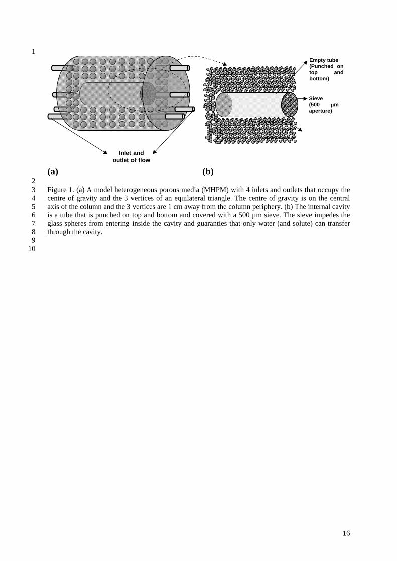
2 Figure 1. (a) A model heterogeneous porous media (MHPM) with 4 inlets and outlets that occupy the 3 centre of gravity and the 3 vertices of an equilateral triangle. The centre of gravity is on the central 4 axis of the column and the 3 vertices are 1 cm away from the column periphery. (b) The internal cavity 5 is a tube that is punched on top and bottom and covered with a 500 µm sieve. The sieve impedes the 6 glass spheres from entering inside the cavity and guaranties that only water (and solute) can transfer 7 through the cavity. 8 9

10

(a) (b)

Inlet and outlet of flow

Empty tube (Punched on top and bottom)

Sieve (500 µm aperture)

17

1 2

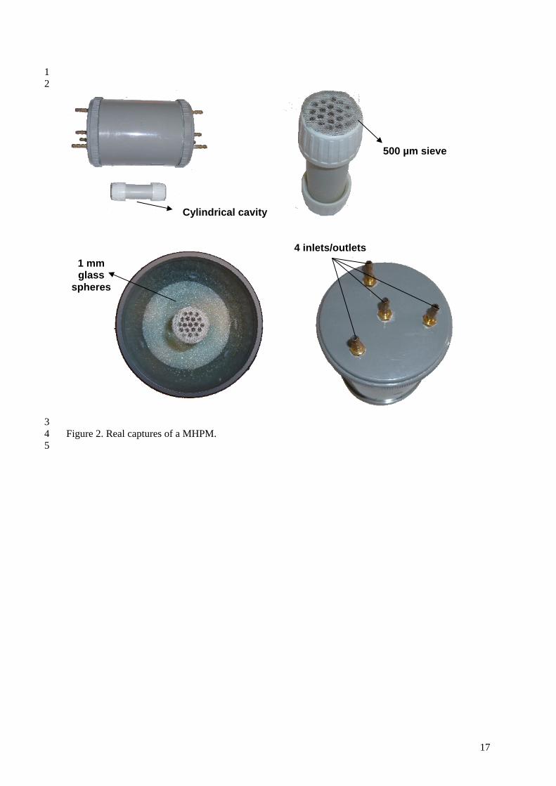
3 Figure 2. Real captures of a MHPM. 4

5

Cylindrical cavity

500 µm sieve

1 mm glass

spheres

4 inlets/outlets

18

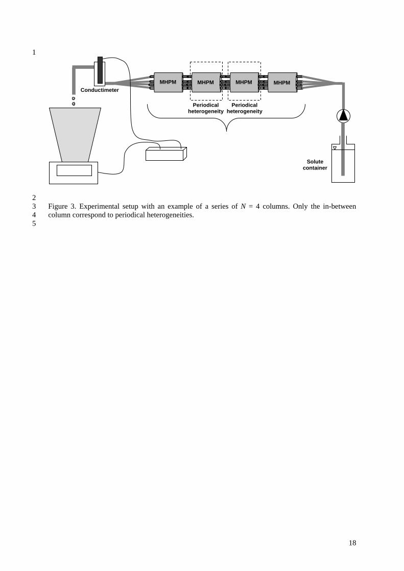
1

2 Figure 3. Experimental setup with an example of a series of N = 4 columns. Only the in-between 3 column correspond to periodical heterogeneities. 4

5

Solute container

Conductimeter

Periodical heterogeneity

MHPM MHPM MHPM MHPM

Periodical heterogeneity

19

1

0

1

0 2000

c* (-)

t (s)

N = 3

min-max

Average

Std dev

-6

-5

-4

-3

-2

-1

0

0 0.1

log P

s (Hz)

N = 3

min-max

Average

0

0

0 3500

c* (-)

t (s)

N = 5

min-max

Average

Std dev

-10

-5

0

0 0.1

log P

s (Hz)

N = 5

min-max

Average

0

0

0 5000

c* (-)

t (s)

N = 10

min-max

Average

Std dev

-20

-15

-10

-5

0

0 0.1

log P

s (Hz)

N = 10

min-max

Average

0

0

0

c*

-30

-25

-20

-15

-10

-5

0log

2 3 Figure 4. Breakthrough curves and the Laplace transforms of their derivatives for N = 3, 5, 10, and 15 4 MHPM. Note the logarithmic coordinates for the Laplace transform. 5

6

20

-4

-3

-2

-1

0

0 0.1

log r

s (Hz)

(a)

(M,N) = (3,5)-4

-3

-2

-1

0

0 0.1

log r

s (Hz)

(b)

(M,N) = (5,10)-4

-3

-2

-1

0

0 0.1

log r

s (Hz)

(c)

(M,N) = (10,15)

-4

-3

-2

-1

0

0 0.1

log r

s (Hz)

(d)

(M,N) = (3,10)-4

-3

-2

-1

0

0 0.1

log r

s (Hz)

(e)

(M,N) = (5,15)-5

-4

-3

-2

-1

0

0 0.1

log r

s (Hz)

(f)

(M,N) = (3,15)-4

-3

-2

-1

0

0 0.1

log r

s (Hz)

(g)

[r1,r2]

1 2 Figure 5. Unit response of a column inferred from the Laplace transforms of the experimental signals. 3

4

21

-3

-2

-1

0

0 0.1

log r

s (Hz)

(a)

N = 1Eq. (6)

-8

-6

-4

-2

0

0 0.1

log r

s (Hz)

(b)

N = 3Eq. (6)

-12

-8

-4

0

0 0.1

log r

s (Hz)

(c)

N = 5Eq. (6)

-20

-10

0

0 0.1

log r

s (Hz)

(d)

N = 10Eq. (6)

-30

-20

-10

0

0 0.1

log r

s (Hz)

(e)

N = 15Eq. (6)

-50

-40

-30

-20

-10

0

0 0.1

log r

s (Hz)

(f)

N = 20Eq. (6)

-80

-60

-40

-20

0

0 0.1

log r

s (Hz)

(g)

N = 30Eq. (6)

1 2 Figure 6. Best AD model fits in the Laplace space for various of N. 3 4