Solitons and Instantons LECTURE NOTES - Cornell...

1

Solitons and InstantonsLECTURE NOTES

Lecture notes largely based on a lectures series given by Csaba Csakiat Cornell University in 2013

Notes Written by: JEFF ASAF DROR

2016

Contents

1 Introduction 5

2 Scalar solitons 62.1 1 + 1 dimensional solitons . . . . . . . . . . . . . . . . . . . . . . . . . . 6

2.1.1 Soliton basics . . . . . . . . . . . . . . . . . . . . . . . . . . . . . 62.1.2 Static solutions . . . . . . . . . . . . . . . . . . . . . . . . . . . . 92.1.3 Explicit solution . . . . . . . . . . . . . . . . . . . . . . . . . . . 112.1.4 Particle-like properties . . . . . . . . . . . . . . . . . . . . . . . . 13

2.2 Complications and topology . . . . . . . . . . . . . . . . . . . . . . . . . 132.2.1 Multiple scalar fields . . . . . . . . . . . . . . . . . . . . . . . . . 142.2.2 Topological charge . . . . . . . . . . . . . . . . . . . . . . . . . . 142.2.3 Derrick’s theorem and D > 1 . . . . . . . . . . . . . . . . . . . . 16

3 Solitons in gauge theories 183.1 Review of gauge fields . . . . . . . . . . . . . . . . . . . . . . . . . . . . 183.2 Non-abelian Higgs theory . . . . . . . . . . . . . . . . . . . . . . . . . . . 193.3 Vacua of spontaneously broken gauge theories . . . . . . . . . . . . . . . 21

3.3.1 Georgi-Glashow model . . . . . . . . . . . . . . . . . . . . . . . . 223.3.2 SU(5) . . . . . . . . . . . . . . . . . . . . . . . . . . . . . . . . . 23

3.4 Topological solutions with SSB . . . . . . . . . . . . . . . . . . . . . . . 243.5 Vortex solution . . . . . . . . . . . . . . . . . . . . . . . . . . . . . . . . 25

3.5.1 Critical Vortex . . . . . . . . . . . . . . . . . . . . . . . . . . . . 29

4 Homotopy Theory 324.1 Basics . . . . . . . . . . . . . . . . . . . . . . . . . . . . . . . . . . . . . 324.2 Important examples . . . . . . . . . . . . . . . . . . . . . . . . . . . . . . 354.3 Exact homotopic sequence . . . . . . . . . . . . . . . . . . . . . . . . . . 38

4.3.1 Basics . . . . . . . . . . . . . . . . . . . . . . . . . . . . . . . . . 384.3.2 Examples . . . . . . . . . . . . . . . . . . . . . . . . . . . . . . . 38

5 Magnetic Monopoles 425.1 Monopoles in general . . . . . . . . . . . . . . . . . . . . . . . . . . . . . 42

5.1.1 Dirac’s derivation . . . . . . . . . . . . . . . . . . . . . . . . . . . 425.1.2 Derivation using quantization of angular momentum . . . . . . . 45

2

CONTENTS 3

5.2 Dyons . . . . . . . . . . . . . . . . . . . . . . . . . . . . . . . . . . . . . 465.3 Duality transformation of Maxwell’s equations . . . . . . . . . . . . . . . 475.4 Topological Monopoles . . . . . . . . . . . . . . . . . . . . . . . . . . . . 48

5.4.1 ’t Hooft-Polyakov monopole . . . . . . . . . . . . . . . . . . . . . 49

Preface

If you have any corrections please let me know at [email protected]. Useful referencesfor this course are Aspects of Symmetry by S. Coleman[1], Solitons and Instantons by R.Rajaraman [2], and ABC of Instantons by M. Shifman et al. [3]

4

mailto:[email protected]

Chapter 1

Introduction

This lecture series will be study of non-trivial field configurations in quantum field the-ories. Conventional quantum field theory (QFT) assumes the classical field we expandaround are independent of space and time. While this is true for the bulk of effects inQFT, there are some states and effects which are due to non-trivial topologies for theunperturbed state. These effects are not small perturbations and thus never be extractedusing a perturbative expansion. We begin by studying these effects in Minkowski space,where we show that additional particles exist in QFT which are not excited states of atrivial classical configuration. Such particles are collectively known as solitons. We thenmove on to studying such solutions in Euclidean space, which provide a description oftunneling phenomena in QFT through what are known as instantons. Tunneling canhave profound effects producing new effective operators into the Lagrangian.

Solitons and instantons are nonperturbative solutions of the classical nonlinear equa-tions of motion. We differentiate the two as follows:

Solitons InstantonsMinkowski Euclidean

Finite energy, E <∞ Finite action, S <∞Non-dissapative, remain localized Not a particle, describes tunneling effect

The similarities of the two are:

• Neither of these two involve an expansion in the coupling constant.

• Topological conservation - there will be a different kind of conserved charge butthis current doesn’t follow from Noether’s theorem.

5

Chapter 2

Scalar solitons

2.1 1 + 1 dimensional solitons

2.1.1 Soliton basics

We begin our discussion with classical scalar field theory in Minkowski space. As inordinary QFT, the classical solutions will be the vacuum for which we quantize ourtheory. Thus understanding the classical solutions is instrumental in understanding thefull quantum theory. To this end we study the Euler-Lagrange equations of motion,

∂µ∂L

∂(∂µφ)=∂L∂φ

(2.1)

As we will see solutions to this equation can vary in space. In order for this solution tohave physical importance, it needs to have a finite energy,

E ≡∫ddxE(x, t) (2.2)

where, E ≡ T 00. Furthermore, we want vacuum states which are stable over time, instead

of converting to trivial solutions at late times. This condition can be written as,

limt→∞

maxall xE(x, t) 6= 0 (2.3)

This is a physicists definition of the soliton. This slightly differs from a mathematiciansdefinition which involves a requirement that the superposition of two solitons remaina soliton. They would call the less restrictive solutions that satisfy the conditions wementioned above, solitary waves.

The crucial aspect of all these solutions is going to be, what is the manifold of vacuafor the theory. If there is no nonlinear term there is nothing nontrivial. We really wantto take the interaction term seriously and add it to the action.

We start with φ4 theory1,

L =1

2∂µφ∂

µφ− 1

4λφ4 (2.4)

1We use the negative spatial metric throughout and gµν = (1,−1) for two dimensions

6

2.1. 1 + 1 DIMENSIONAL SOLITONS 7

The equation of motion for this theory is ( ≡ ∂µ∂µ),

φ+ λφ3 = 0 (2.5)

Our goal is to find solutions this partial differential equation with finite energy. Insteadof attacking this problem head-on, lets first compute the energy. The potential is just aquartic,

φ

V (φ)

The energy momentum tensor is found by considering the variation of the Lagrangianunder space-time translations which gives,

T µν = ∂µφ∂νφ−1

2(∂µφ)2δµν +

λ

4φ4δµν (2.6)

allowing us to compute the energy density (we use a prime to indicate a spatial derivative)

E =1

2φ2 +

1

2φ′2 +

λ

4φ4 (2.7)

The energy of the given solution is,

E [φ] =

∫ ∞−∞

dx

(1

2φ2 +

1

2φ′2 +

λ

4φ4

)(2.8)

Here we are working in 1 + 1 dimensions. The energy is clearly positive definite. Theenergy is zero only if φ = 0. But we are not requiring zero energy solutions, we are justrequiring finite energy solutions. Can we find other finite energy solutions? In this case,no. Here we have only 1 classical vacuum. To get a finite energy, we must have φ → 0for x→ ±∞. While field configurations that start and end with the same value of φ aresolutions, it turns out there are no non-trivial solutions with these boundary conditions(we show this rigorously later on).

Now instead lets consider a theory with two vacua:

8 CHAPTER 2. SCALAR SOLITONS

φ

V (φ)

A sample potential is given by,

V (φ) =1

2∂µφ∂

µφ+1

2φ2 − λ

4φ4 (2.9)

Then the energy density expression then is,

E [φ] =

∫ ∞−∞

dx

(1

2φ2 +

1

2φ′2 − 1

2φ2 +

λ

4φ4

)(2.10)

The minima occur at φ± = ±1/√λ. Then the condition to have finite energy solutions

is,lim

x→±∞φ→ φ± (2.11)

This problem has less trivial boundary conditions and can yield non-trivial solutions.Instead of study the two previous cases in detail, lets consider an arbitrary potential.

A Lagrangian with a potential, U(φ) is given by,

L =1

2(∂µφ)2 − U(φ) (2.12)

with U(φ) being some complicated function,

φ

U(φ)


There are many possible positions where the potential is vanishing. If we denote theminima with φi then we have U(φi) = 0. The equation of motion is given by,

φ− φ′′ = −∂U∂φ

(2.13)

The energy density is given by,

E [φ] =

∫ ∞−∞

dx

[1

2φ2 +

1

2φ′2 + U(φ)

](2.14)

E [φ] = 0 implies that the field is constant, φ = φi. Alternatively finite solutions can beacheived if scalar field asymptotically approaces on of the vacua. Therefore, E [φ] < ∞implies that,

limx→+∞

φ = φi, limx→−∞

φ = φj (2.15)

The finite energy solutions interpolate between two of the zeroes in the potential.We now want to find explicit form for these solutions. Solving the partial differential

equation is difficult, but we can simplify our analysis using Lorentz invariance. Insteadof solving the full equations we can first look for static solutions and then add the timedependence by boosting them 2.

2.1.2 Static solutions

The equation of motion in the static case is,

φ′′ =∂U

∂φ(2.16)

This is an ordinary second order differential equation. This is reminiscent of Newton’ssecond law for a 1D particle in a potential with the sign of the potential is reversed,x = −∂U

∂x.

φ

−U(φ)

2Its not apriori clear whether there are some additional time dependent solutions that we can’t getfrom boosting them. While we acknowledge this as a possibility we ignore it for our purposes.


As in Newton’s equation we can introduce a conserved quantity, the “total mechanicalenergy”,

W =1

2φ′2 − U (2.17)

You know that when x→ ±∞ the field has to approach a constant value (its at minimumof the potential). This implies that φ′ → 0. Futhermore, at a zero of the potential weknow that U = 0. Hence to get the finite field theory energy solutions, the mechanicalenergy has to be zero,

limx→±∞

W = 0 (2.18)

Furthermore, since this quantity is conserved we have,

1

2φ′2 = U ⇒ φ′ = ±

√2U(φ) (2.19)

What sort of solutions could this equation yield? You are interested in the mechanicalsolutions in this potential that go from one maximum (in this inverted potential) toanother maximum. This could be something that goes from φmax1 → φmax2 , φmax2 → φmax3 ,etc, where we denote the different maxima by φmaxi .

Claim 1. In 1D, you can only have solutions that go between neighbooring vacua.

Proof. If you try to go from φmax1 → φmax3 then you can only do it by going through φmax2 .When you go through φmax2 you will have U(φmax2 ) = 0. Because this is a maximum thederivative is also vanishing, ∂U(φmax2 )/∂φ. This is telling us that,

1

2φ′2 − U(φ) = 0⇒ φ′ =

√2U(φ) (2.20)

which implies that at the minima, φ′ = 0. Now

φ′′ =∂U

∂φ

∣∣∣∣φ=φmax2

= 0 (2.21)

Furthermore,

φ′′′ =d

dx

∂U

∂φ=∂2U

∂φ2φ′

φmax2−−−→ 0 (2.22)

and similary for higher derivatives. Thus the particle really gets stuck there. You cannotroll down on the other side. In higher dimensions you can avoid a vacua by going aroundit making this feature only present in the one dimensional case.

Lets now address a claim we made earlier:

Claim 2. Any solution with the same initial and final vacuum is a trivial solution.

Proof. Suppose we had a solution that started and ended at the same vacuum, φ0, butmoved away from that vacuum away from infinity. The field starts at φ0 and at somepoint, φ1, it needs to turn around to return to φ0. At the turnaround point we must haveφ′1 = 0, but this implies that U(φ1) = 0 by equation 2.19 and hence φ1 is a vacuum andhence the field will be stuck there.


For n minima you can have the possible transitions,

n−1︷︸︸︷1→ 2 , 2→ 3 , ... , n− 1→ n

n−1︷︸︸︷n→ n− 1 , n− 1→ n− 2 , ... , 2→ 1

Thus in total we have

2(n− 1) (2.23)

possible solutions. The ones that go one direction you call solitons and the ones going inthe other direction are called antisolitons.

2.1.3 Explicit solution

To get an explicit solution we need to integrate over the equation of motion,

1

2φ′2 = U(φ) (2.24)

Separating variables gives,

x− x0 = ±∫ φ(x)

φ0

dφ1√

2U(φ)(2.25)

We now consider the kink solution. This is a 1 + 1 dimensional soliton with thepotential,

U(φ) =λ

4

(φ2 − m2

λ

)2

(2.26)

The higher dimensional version of these are domain walls The way the constant is pickedλ is still the quartic and m is the “mass” of the quantized field. The vacua are at,

φ0 = ±√m2

λ(2.27)

We plug this into our general expression,

x− x0 = ±√

2

λ

∫ φ(x)

φ0

dφ

(φ2 − m2

λ

)−1(2.28)

Lets pick x0 to be the center of the soliton. We can pick where exactly the center of thesoliton is. We pick φ0 = φ(0) = 0.

The integral is easy to perform using Mathematica,∫ x

0

dx1

x2 − a2= −1

atanh−1

x

a(2.29)


Using this result we get (with a = m/√λ),

x− x0 = ±√

2

mtanh−1

(φ(x)

√λ

m

)(2.30)

which gives,

φ(x) = ± m√λ

tanh

[m√

2(x− x0)

](2.31)

This is our first explicit soliton solution. It takes the form,

φ(x)

x

− m√λ

m√λ

pert. vacuax0

antikink

kink

Its obvious that we can’t call this field configuration a particle as its not localized inspace. However, nobody really cares about the fields (perturbative vacua aren’t localizedeither!). Its only the energy density that needs to be localized. This determines if youcan have a particle-like behavior or not.

The energy density is,

E(x) =1

2φ′2 + U(φ) (2.32)

We have,

φ′ =m√λ

1

cosh2[m√2(x− x0)

] (2.33)

1

2φ′2 =

m4

4λ

1


] (2.34)

The total energy density is just,

E(x) =m4

2λ

1


] (2.35)

This is indeed localized as desired,

2.2. COMPLICATIONS AND TOPOLOGY 13

E(x)

xx0

∆L = 1m

To assign some classical mass we would find the total energy,

M ≡ E =

∫ ∞−∞

dxE(x) =2√

2

3

m3

λ(2.36)

Note that λ here is not dimensionless since we are not working in 3+1 dimensions, so thisdoes indeed have dimensions of mass. We see that the mass, M ∝ 1

λ. This is something

you will never get in perturbation theory.

2.1.4 Particle-like properties

To get the solution for all times can boost this solution,

x− x0 → γ(x− x0 − vt) , (2.37)

γ ≡ (1− v2)−1/2. Boosting the field,

φ→ ± m√λ

tanh

[γm√

2(x− x0 − vt)

](2.38)

with an energy density,

E =γm4

2λsech4

[γm√

2(x− x0 − vt)

](2.39)

Performing the integral over space gives as expected,

E = γM (2.40)

2.2 Complications and topology

We now consider more complicated soliton solutions.


2.2.1 Multiple scalar fields

First suppose we have multiple scalar fields,

φi(x, t) i = 1, ..., N (2.41)

with the Lagrangian and equations of motion:

L =1

2φi 2 − 1

2φi ′ 2 − U(φi) ⇒ φi = −∂U

∂φi(2.42)

Static solutions can be found from,

φi ′′ =∂U

∂φi(2.43)

The classical mechanical analogue is a N -dimensional motion of particle in −U(φi) po-tential. The total energy is,

E[φi]

=

∫dx∑i

φi ′ 2 + U(φi) (2.44)

The main difference here is that we can have a non-trivial solutions iwth one minimumfor the potential. For example:

φ2

φ1

×φ0

2.2.2 Topological charge

In both cases we’ve seen so far there is an important quantity which characterizes thefield configuration, the difference in the vacuum at spatial infinity. We claim this is aconserved quantity suggesting the following definition:

Def. 1. Topologically Equivalent: Two solutions are said to be topologically equivalentif they cannot be continuously deformed into one another without passing through a barrierof infinite action.

Def. 2. Continuous Deformation: For two solutions, f1(x) and f2(x), a continu-ous deformation, parameterized by t ∈ [0, 1], between the two solutions is a continuousfunction, F (t, x), such that F (0, x) = f1(x) and F (1, x) = f2(x).


Are the two kink solutions topologically equivalent? To check this we introduce ageneric deformation,

Φ(t, x) =m√λ

[g(t) tanh y + h(t) tanh(−y)] y ≡ m√2

(x− x0) , (2.45)

= (g − h)m√λ

tanh y , (2.46)

where g, h are arbitrary continuous functions of t with g(0) = h(1) = 1 and g(1) = h(0) =0. The static action is given by,

S(t) =

∫dx

1

2Φ′ 2 +

λ

4

(Φ2 − m2

λ

)2

(2.47)

=m4

4λ

∫dx(g − h)2

1

cosh4 y+((g − h)2 tanh2 y − 1

)2(2.48)

The first integral is convergent, however the second diverges for |g(t) − h(t)| 6= 1. Wehave g(0)−h(0) = 1 and g(1)−h(0) = −1. and since g and h are continuous, there mustbe a point in t ∈ (0, 1) for which the integral diverges. Thus we conclude that these twosolutions are topologically inequivalent.

Thus at least for the kink the quantity,

φ(∞, t)− φ(−∞, t) (2.49)

cannot be changed with a finite amount of energy and must be conserved. We will alwaysassume that the non-trivial topological solutions we find are topologically inequivalent.Thus we can define a quantity known as the “topological charge” that quantifies thedifference between vacua:

Q ∝ φ(∞, t)− φ(−∞, t) , (2.50)

where the constant of proporitionality is conventional. For the kink one can introduce,

Q ≡√λ

m(φ(∞, t)− φ(−∞, t)) (2.51)

Thus,

Q =

2 (kink)

0 (trivial)

−2 (anti-kink)

(2.52)

Note that this charge does not follow from Noether’s theorem, but instead is conservedindependently from the equations of motion. Since we have a conserved charge, we expectsome associated current. We can find the current by rewriting the charge,

Q =

√λ

m

∫dx∂xφ(x, t) (2.53)


Thus we know that j0 =√λm∂xφ. We want to make this into a four-vector. The only

tensors we have at our disposal are gµν , εµν , and ∂µ. Thus we must have,

jµ =

√λ

mεµν∂νφ (2.54)

This is divergenceless as required, ∂µjµ ∝ εµν∂µ∂νφ = 0.

2.2.3 Derrick’s theorem and D > 1

We now consider solitons in more than one spatial dimension, D. In such systems thereis a theorem, known as Derrick’s theorem, which restricts the type of systems thatcan have topological solutions. Consider a N -component scalar field, φi(x, t) in D spatialdimensionn. The Lagrangian is given by,

L =1

2∂µφ

i∂µφi − U(φi) (2.55)

The static equations of motion are the solutions of the equation,

φi =∂U

∂φi(2.56)

with static energy,

E =

∫dDx

1

2∂aφ

i∂aφi︸︷︷︸

≡E1[φi]

+

∫dDxU(φi)︸︷︷︸≡E2[φi]

(2.57)

Now lets assume we find φi1 which is a solution of the equations of motion. Now considerthe class of field configurations (which are generically not solutions),

φiλ(x) ≡ φi1(λx) (2.58)

The action for a given solution φλ(x) is given by,

S(λ) = −∫dDx

(1

2∂aφ

i1(λx)∂aφ

i1(λx) + U

[φi1(λx)

])(2.59)

= −∫dDyλ−D

(1

2λ2

∂

∂yaφi(y)

∂

∂yaφi(y) + U [φ1(y)]

)(2.60)

= −(λ2−DE1 + λ−DE2) (2.61)

To have an extremum of the action,

dS(λ)

dλ= (2−D)λ1−DE1 −Dλ−D−1E2 = 0 ⇒ E2 =

2−DD

E1 (2.62)

Now the key observation, is that E1 and E2 are both positive definite quantities. Thisputs a restriction on the possible values of D. To this let us consider the different cases:


1. D = 1: In this case we find, E1 = E2. This says that in one spatial dimension thetension in the field is equal to its potential energy. This is an analogue to the viraltheorem.

2. D = 2: This says that E2 = 0 or equivalently, U = 0. The only known possibilitywhere you have a non-trivial solution is in the non-linear σ model where φiφi = a2.

3. D > 2: E2 < 0! since E2 is positive definite, there are no non-trivial solutions forD > 2.

Thus, the somewhat dissapointing conclusion is that in the 3 + 1 dimensions scalar fieldscannot have instanton solutions. Note that its still possible to lift lower dimensionalsolutions to 3 + 1 dimensions but these won’t be finite energy and hence do not have aparticle interpretation (e.g., domain walls).

Chapter 3

Solitons in gauge theories

3.1 Review of gauge fields

Before plunging into solitons in gauge theories we quickly review the basics of non-abeliangauge theories. A group G is charactorized by the structure constants, fabc, which arerelated to the generators of the group by,[

T a, T b]

= −ifabcT c (3.1)

and a = 1, 2, ..., dim(G). The gauge fields are denoted by,

Aµ ≡ AaµTa (3.2)

and the fields transform under the gauge symmetry through,

Aµ → gAµg−1 +

i

e(∂µg)g−1 (3.3)

where e denotes the coupling constant, and g is a group element in the adjoint represen-tation,

g ≡ eiαaTa (3.4)

Explicitly we can write the gauge transformation in terms of the generators:

gAµg−1 = eiαaTaT be−αcTcAb (3.5)

= Aµ + iαa (TaTb − TbTa)Ab + ... (3.6)

= Aµ + αafabcTcAbµ (3.7)

Furthermore,

1

2(∂µg)g−1 =

i

e(i∂µαaTa) (1− αaTa) (3.8)

= −1

e∂αaTa (3.9)

18

3.2. NON-ABELIAN HIGGS THEORY 19

Therefore,

Aµ → Aµ −1

e∂αaTa − εafabcTcAb (3.10)

Under a gauge transformation the field strength tensor,

F aµν = ∂µA

aν − ∂νAaµ − efabcAbµAcν (3.11)

transformations in the adjoint representation,

Fµν → gFµνg−1 (3.12)

3.2 Non-abelian Higgs theory

We now consider a non-abelian gauge theory with a Higgs field in a generic representation.The Lagrangian is given by,

L = −1

4TrFµνF

µν + |Dµφ|2 + U [φ] (3.13)

with the covariant derivative,

(Dµφ)m = ∂µφm + ieAaµtamnφn (3.14)

Computing the equations of motion is straightforward. The final result is,

DµFaµν = ieφtaDνφ+ h.c. (3.15)

DµDνφm =

(∂U

∂φm

)∗(3.16)

We now look for static solutions,

∂0φ = 0 (static) (3.17)

Claim 3. There exists a gauge such that A0 = 0. This is known as the temporal gauge.

Proof. Consider a generic gauge configuration and apply a gauge transformation,

A0 → gA0g−1 +

i

e(∂0g)g−1 (3.18)

We need to show there exists a g such that,

gA0g−1 = − i

e(∂0g)g−1 (3.19)

for any A0. This condition can be rewritten,

g−1∂g

∂t= ieA0 (3.20)

20 CHAPTER 3. SOLITONS IN GAUGE THEORIES

This is a well known diffential equation, familiar from constructing correlation functionsin QFT, and has the solution,

g = T exp

[ie

∫A0(t

′)dt′]

(3.21)

Thus for static solutions we can always work in a gauge such that,

D0φ = 0 (static) (3.22)

Note that this still does not completely fix the gauge as we can still make t-indepentgauge transformations.

In this gauge fixing,

F a0i = ∂0A

ai − ∂iAa0 − efabcAb0Aci = ∂0A

ai (3.23)

which gives the action,

S =

∫dDx

[1

2(∂0A

ai )

2 + |∂0φ|2]

+

∫dDx

[1

4(F a

ij)2 + |Diφ|2 + U [φ]

](3.24)

= 0 + E1

[F 2]

+ E2 [Diφ] + E3 [U ] (static) (3.25)

Using this we can now rebuild the scaling arguement in the theory.Assume we found a static solution to the equations of motion,

φ1(x) , Aµ1(x) (3.26)

Now consider the family of functions which are not solutions to the equations of motion,except at λ = 1:

φλ(x) = φ1(λx) , Aµλ(x) = λAµ1(λx) (3.27)

which implies,Fij(x)→ λ2Fij(λx) , Diφ→ λDiφ(λx) (3.28)

This gives a rescaled action,

S [φL, Aµλ] = −λ−D

∫dD(λx)

1

4λ4Fij(λx)Fij(λx) + λ2 |Diφ|2 + U(φ) (3.29)

= −λ−D(λ4E1 + λ2E2 + E3

)(3.30)

As before we should have an extremum in the action when λ = 1:

−Dλ−D−1(λ4E1 + λ2E2 + E3

)+ λ−D

(4λ3E1 + 2λE2

)= 0 (3.31)

or(4−D)E1 + (2−D)E2 −DE3 = 0 (3.32)

As before, lets consider the different cases

3.3. VACUA OF SPONTANEOUSLY BROKEN GAUGE THEORIES 21

1. D = 1: Gauge fields don’t propagate with one spatial dimension, so we don’t expectany interesting instanton effects here

2. D = 2: Our master equation tells us that E1 = E3. For this peculiar possibility,the scalar potential energy is exactly equal to the gauge field energy. This is knownas the “vortex” solution.

3. D = 3: The master equations says that E1 − E2 − 3E3 = 0. This corresponds to amonopole solution.

4. D = 4: Here the master equations gives, −2E2 − 4E3 = 0. This can only be asolution if E2 = E3 = 0. In other words in four spatial dimensions soliton solutionscan exist only if the scalar field has vanishing energy ⇒ solution involves only thegauge field. These will be of fundamental importance when we discuss instantonsbut we postpone this discussion until then.

3.3 Vacua of spontaneously broken gauge theories

We now study the vacuum of a gauge theory with a manifold of vacua, instead of finiteset of discrete vacua. The concept of a manifold of vacua is familiar from spontaneouslybroken symmetries. Since we are interested in D = 3, we study theories with scalarand gauge fields. Both of these will have a non-trivial vacuum configurations. Theperturbative vacuum is simmply,

φ0 = const , Aaµ = 0 (3.33)

However, our interest will be in more intricate vacua.

Consider the gauge group, G (with elements, g), broken to a subgroup, H (withelements h). We denote a vacuum state by φ0. Since the vacuum is invariant under thesubgroup we have,

hφ0 = φ0 (3.34)

Gauge fields in H will remain massless and the other gauge bosons (those in G/H) pickup a mass. U(φ) must be invariant under, φ→ gφ, which in turn also implies,

U(gφ0) = 0 (3.35)

Thus the set of vacua related to φ0 by a full gauge transformation correspond to minima.While gφ0 always corresponds to a minima its non-trivial to know whether this willcorrespond to all minima.

Claim 4. If gφ0 can generate all minima than the minimal set of generators that cangenerate all minima, is the “coset”, G/H, defined by g1 = g2h.


Proof. Let us parameterize all minima by a vector, θ: φ0(θ). By assumption it is givenby a group element acting on a single vacuum,

φ0(θ) = g1φ0(0) (3.36)

Generically this choice of g will not be unique and so we’ll also have

φ0(θ) = g2φ0(0) (3.37)

This implies that,

g−12 g1φ0(0) = φ0(0) (3.38)

which is the defining characteristic of the unbroken subgroup. Thus,

g−12 g1 = h ⇒ g1 = g2h (3.39)

Thus the elements g which are identified with g1 = g2h can generate all the minima.

One subtlety to the above is sometimes the invariance of the potential (G) is a bitbigger than that of the full gauge group, G. Then subgroup may also be a bit smaller, H.What you are really after is G/H. We will see an example of this shortly when considerSU(5).

3.3.1 Georgi-Glashow model

The Georgi-Glashow model was a candidate for the weak interactions before the confir-mation of the Z boson. The model comprises of SU(2) gauge symmetry with a Higgstriplet, φa and a potential,

U =λ

4

(φiφi − a2

)2(3.40)

The symmetry of the potential is, SU(2).

Claim 5. SU(2) is isomorphic to S3 (3D sphere embedded in 4D)

Proof. An arbitrary element of SU(2) can be written as,(a b−b∗ a∗

)(3.41)

with the condition |a2|2 + |b|2 = 1. Writing a = y1 + iy2 and b = y3 + iy4 gives thecondition,

y21 + y22 + y23 + y24 = 1 (3.42)

which is the defining equation for 3-sphere.

3.3. VACUA OF SPONTANEOUSLY BROKEN GAUGE THEORIES 23

The Higgs gains a vacuum expectation value (VEV) which by gauge symmetry canbe taken to be in the first component,

φ =

h+ aφ2

φ3

(3.43)

Then,

V =λ

4

(φ22 + φ2

3 + 2ha)2

(3.44)

The h field is massive and φ2 and φ3 are massless giving 2 goldstone bosons (GB). Theinvariant subgroup is H = SO(2) and corresponds to rotations between φ2 and φ3. Thevacuum manifold is given by SU(2)/U(1) which is a 2-sphere, S2 (a sphere embedded ina 3 dimensional space). This is because the vacua are characterized with,

φ21 + φ2

2 + φ23 = a2 (3.45)

which is the defining equation of a 2-sphere.

φ21 + φ2

2 + φ23 = a2

φ3

φ2

φ1

3.3.2 SU(5)

Next consider G =SU(5), a candidate for grand unification of the SM, broken by ascalar adjoint Higgs, φ, to SU(3)×SU(2)×U(1). A scalar adjoint can be formed from afundamental and anti-fundamental, forming a hermitian tracless 2×2 matrix transformingas φ → gφg−1. Usually the potential which gives rise to this breaking has an accidentalZ2 symmetry under the transformation,

φ→

−1

−1−1

−1−1

φ (3.46)


This is not an element of SU(5) (it doesn’t have determinant equal to 1). Thus thepotential is invariant under

G = SU(5)× Z2 (3.47)

An adjoint of the VEV,

φ0 = v

1

11−3/2

−3/2

(3.48)

can produce the desire symmetry pattern. H is made of,M1 ≡

(g1

12×2

), M2 ≡

(13×3

g2

), M3 ≡

(e2iθ13×3

e−3θ/212×2

)(3.49)

Clearly,Hφ0 = hφh−1 = φ0 (3.50)

as desired. However, not all of the vacua at distinct, e.g., g1 = e−2π/313×3, g2 = −12×2,θ = π/3. Then

M1M2M3 = 15×5 (3.51)

Therefore, the invariance group is not SU(3)×SU(2)×U(1) but smaller. One can showthat the actual subgroup is SU(3)× SU(2)× U(1)/Z6. This will effect properties of themonopole!

3.4 Topological solutions with SSB

We now repeat the procedure to find topological solutions. As before we work in thetemporal gauge. Furthermore, it will be convenient to work in polar coordinates. Weclaim without proof that one can use the remaining gauge freedom to fix the gauge suchthat,

Aar = 0 (3.52)

In order to have a finite energy density we must have,∫dDx |Diφ|2

r→∞−−−→ 0 (3.53)

Due to our gauge fixing condition this implies,

∂rφr→∞−−−→ 0 (3.54)

and so φ will asymptotically be r independent,

φ∞(r, θi, t) = φ∞(θi, t) (3.55)

3.5. VORTEX SOLUTION 25

The field values at∞ are called the “sphere at infinity”. We learned from our experiencewith solitons that different vacuum configurations of the field at the boundaries, yieldsdifferent topological solutions. Thus this sphere at (spatial!) infinity, should somehow bemapped to the different vacua. In D spatial dimensions this implies a mapping,

SD−1 → G/H (3.56)

The mathematical tool to compute these mappings is known as “homotopy theory”,which we’ll study in more detail soon. However, in many cases you can use physicalarguments to compute most of what you need to understand the topology, as we did forSU(2)→ U(1) where we found we needed a mapping from S2 → S2.

Our goal is to find non-trivial classical solutions to the equations of motion. Thus wewant the derivatives of the fields to be non-vanishing. However, equation 3.53 combinedwith equation 3.54, greatly restrict the possible solutions! We must have,

limr→∞

Dθiφ = limr→∞

1

r

1

sin θ...

∂φ∞∂θi

+ iAθiφ∞ = 0 (3.57)

Since φ is asymptotically r-independent, we know how Aθi behaves at large r:

limr→∞

Aθi ∝1

r(3.58)

Recall that we are interested in finite action solutions. For a potential falling off as 1/ris the energy in the E and B fields finite? Equation 3.24 shows that the energy in ourgauge is,

1

4

∫dDx(F a

ij)2 ∼

∫dD−1θ

∫drrD−1

1

r4(3.59)

which is convergent if D − 5 ≤ −2 or D ≤ 3. Thus we conclude:

Finite action, non-trivial, solutions to the classical equations of motion can onlyexist in spontaneously broken gauge theories if D ≤ 3.

3.5 Vortex solution

The vortex is a topological solution of a spontaneously broken abelian gauge symmetry,also known as “Landau-Ginsburg” theory. We will focus on the case of 2+1 dimensions,known as the Neilson-Oloson vertex. It has important physical consequences as it forms atheory of superconductivity through a dynamical breaking of U(1)EM which occurs throghcondensation of electron pairs giving a non-zero vacuum expectation value,

〈Ω|e−e−|Ω〉 6= 0 (3.60)


The unbroken group is G = U(1) with a complex scalar, φ, which in superconductivity,forms the electron pair: φ ≡ 1

f2e−Le

−R, where f is some dimensionful scale. We will take

the scalar potential to be,

V (φ) =λ

4

(|φ|2 − a2

)2λ > 0 (3.61)

The vacuum manifold (parametrized by G/H = U (1) ' S1) is given by,φ0(σ) = aeiσ

(3.62)

Since we are working in 2 spatial dimensions, the sphere at infinity is also a circle,

φ(∞, θ) : S1 → S1 (3.63)

To describe the boundary conditions we need a mapping between θ → σ, i.e., we needσ(θ). Pictorally,

sphere at ∞mapping

σ(θ)

We are interested in homotopically inequivalent mappings.

Def. 3. Homotopically Equivalent: Two mappings, σ1(θi) and σ2(θi) are homotopi-cally equivalent if there exists a linear combination of the mappings with a parameter tsuch that at t = 0 its equal to σ1 and at t = 1 its equal to σ2 while keeping the base-pointfixed.

Def. 4. Based point: A base point of a mapping, σ(θi) is reference point of the mappingwhere σ(θi,0) is always equal to some constant, σ0

Before studying this model in detail lets give a few examples. First consider themappings,

σ1(θ) = θ σ2(θ) = kθ, k ∈ Z (3.64)

The basepoint we have chosen is θ0 = 2πp, σ0 = 2πp, p ∈ Z. Clearly both these solutionsobey this condition. Are these homotopically equivalent? Consider,

tσ1(θ) + (1− t)σ2(θ) = [k + t(1− k)] θ (3.65)

This homotopy does not keep the basepoint fixed unless k = 1 for all t and hence thesesolutions are not homotopically equivalent. We see that solutions which go around thesphere at infinity a different number of times are homotopically equivalent.


Alternatively, consider two mappings which both go around the sphere at infinity withdifferent “speeds”:

σ1(θ) = θ σ2(θ) = 2π sinθ

4(3.66)

These are homotopically eqiuvalent since,

tσ1(2π) + (1− t)σ2(2π) = 2π (3.67)

and hence keeps the basepoint fixed.Lastly consider the trivial mapping and a mapping which doesn’t go once around the

vacuum:

σ1(θ) = 0 σ2(θ) =

θ 0 ≥ θ ≥ π

(2π − θ) π ≥ θ ≥ 2π(3.68)

The linear combination:tσ1(2π) + (1− t)σ2(2π) = 0 (3.69)

and so these are homotopically equivalent.We see that the key concept in finding charatorizing mappings is the number of

times we go around the circle in coset space as we go once around the circle at infintiy.This is known as the winding number. The above consider show1 that mappings arehomotopically inequivalent if and only if they have the different winding numbers. Aswe’ll see there is an infinite number of such solutions, each having a distinct energy.

Explicitly, the winding number can be written,

n =σ(2π)− σ(0)

2π(3.70)

=1

2π

∫ 2π

0

dθdσ(θ)

dθ(3.71)

We can compute the action explicitly for the vacuum manifold, φ = aeiθ. The action isgiven by,

−∫d2x

[1

4FijF

ij + |Diφ|2 + U(φ)

](3.72)

For static solutions the energy is always equal to the negative of the action. Thus toavoid keeping track of a pesky negative sign, we’ll always work with the energy and lookfor extrema in the energy instead. Since we are working with an abelian 2D gauge theorywe can simplify the gauge field:

F12 = ∂xAy − ∂yAx = εij∂iAj = B (3.73)

At r →∞,φ(∞, θ) = aeiσ(θ) (3.74)

1Technically we didn’t actually show that solutions with different winding numbers are homotopicallyinequivalent since we only tried one candidate mapping.


Inserting this into equation 3.57 we get,

limr→∞

Dθφ = limr→∞

(ari∂θσ − ieAθa

)eiσ = 0 (3.75)

or,dσ

dθ= e lim

r→∞rAθ (3.76)

Note that earlier we concluded that Aθ ∝ 1r

so this is a finite quantity. This can be usedto compute the winding number:

n =e

2π

∫ 2π

0

dθ limr→∞

rAθ (3.77)

=e

2π

∫A · ds (3.78)

=e

2π

∫B · da (3.79)

This is just the magnetic flux passing through the circle at infinity giving the quantizationcondition,

Φ =2π

en (3.80)

Thus we conclude that for n 6= 0 this theory has quantized magnetic charge. This isindeed the case in a superconductor.

Lets pause and summarize what happened here. We studied the classical solutionsto a 2+1 dimensional spontaneously broken U(1) gauge theory and looked for solutionswith non-trivial vacua and finite energy. We found that there exists an infinite set of suchsolutions, described by a discrete quantum number: the winding number. There will alsobe solutions with trivial vacua, such that the quantum theory contains excitations ofan ordinary scalar field, an ordinary massive gauge field, and of a novel ground state,whose gauge field configuration produces a non-zero magnetic flux. In a quantum theorythere will be small fluctuations about this vacuum. However, these small fluctuations(by definition of being small) won’t be able to take your out of this vacuum. Thus thisquantity is a conserved quantity often referring to as a topological charge.

Since we have a charge there should be a corresponding current. We want somethingwhich obeys, ∂µj

µ = 0 and which yields,∫d2xj0 = − e

2π

∫d2xεij∂iAj (3.81)

= − e

2π

∫d2xε0µν∂µAν (3.82)

which suggests,

jµ ≡ e

2πεµνρ∂νAρ (3.83)

∂µjµ = 0 as a consequence of the antisymmetry of the levi-cevita desired.


3.5.1 Critical Vortex

Obtaining solutions to the coupled, second order, partial differential equations for φ andAµ is a difficult problem. It would be much nicer if we could reduce these equations tofirst order as we did for the kick solution. Unfortunately, this cannot be done in generalbut we can recast the solutions into a more convenient form in a certain limit. The idea isto use that solutions will minimize the action. If we write the action in terms of positivedefinite quantities we can have a better idea of when the action will be minimized.

Consider the action of the static solution,

E =

∫d2x

[1

2F 212 + |D1φ|2 + |iD2φ|2 +

λ

4

(|φ|2 − a2

)2](3.84)

where we write the kinetic term in a form convenient for the discussion below. The massesof the radial mode and the gauge boson are, m2

A = 2e2a2 and m2φ = 1

2λa2, respectively.

Shifting terms around in the action gives,

E =

∫d2x

[1

2

(F12 +

√λ

2(|φ|2 − a2)

)2

+ |(D1 + iD2)φ|2 − i((D1φ)†D2φ− (D2φ)†D1φ

)−√λ

2F12(|φ|2 − a2)

](3.85)

Using,2 ∫d2x(D1φ)†D2φ− (D2φ)†D1φ = ie

∫d2xφ†F12φ (3.86)

we have,

E =

∫d2x

[1

2

(F12 +

√λ

2(|φ|2 − a2)

)2

+ |(D1 + iD2)φ|2 +

(e−√λ

2

)|φ|2 F12

]+

√λ

2a2Φ

(3.87)

The first two terms are positive definite. The last term is a (quantized) topological term.The third term gives the coupling between the scalar and the gauge boson and its sign,which can be positive or negative depending on the relative value of λ and e, has a crucial

2Note that, ∫d2x(Diφ)†Djφ =

∫d2x(−φ†∂i + ieφ†Ai)Djφ = −

∫d2xφ†DiDjφ

and

F12 =i

e[D1, D2]


effect on the qualitative features of the model. The relevant ratio is an order parameterand can be written in terms of the masses,

mφ

mA

=

√λ/2

e(3.88)

If mφ < mA then we have a type I supeconductor. Here the vortices attact each otherdestropying superconductivity relatively quickly. If mφ > mA then we have a type IIsuperconductor. Here the vortices repel and don’t combine together. This leads to amuch larger critical magnetic field.

To get the rough behavior of the solutions its interesting to consider the regime thatmφ = mA, known as the critical vortex. In this case the total energy is just,

E =

∫d2x

[1

2

(F12 +

√λ

2(|φ|2 − a2)

)2

+ |(D1 + iD2)φ|2]

+ 2πna2 (3.89)

We can now reduce the corresponding second order equations by making a bold assump-tion: the solutions to the equations of motion will minimize these positive definite quanti-ties, lets assume that the terms are identically zero. In this case we get the correspondingequations known as the BPS equations:

F12 + e(|φ|2 − a2

)= 0 (3.90)

(D1 + iD2)φ = 0 (3.91)

For simplicity lets focus on the case where n = 1. We want to use an satz consistent withour boundary conditions,

φ(∞, θ) = aeiθ (3.92)

limr→∞

rAθ =1

e(3.93)

and φ,Aθ finite as r → 0. This gives the generic form,3

φ(r, θ) = aeiθϕ(r) (3.94)

Aθ(r, θ) =1

e

1− f(r)

ror Ai =

1

e

εijxj2r2

(1− f(r)) (3.95)

3Recall that to convert from cartesian to polar coordinates:(AxAy

)=

(cθ −sθsθ cθ

)(ArAθ

)(∂x∂y

)=

(cθ −sθsθ cθ

)(∂r1r∂θ

)


The field strength is given by,

eF12 = eεij∂iAj (3.96)

=1

2∂k

[xk

1− f(r)

r2

](3.97)

= −1

2

1

r

∂f

∂r(3.98)

and

(D1 + iD2)φ = eiθ (Dr + iDθ) aeiθϕ(r) (3.99)

= ae2iθ[∂rϕ(r)−

(1

r− eAθ

)ϕ

](3.100)

= ae2iθ[∂rϕ(r)− f(r)

rϕ

](3.101)

which leads to the BPS equations:

1

rf ′ − 2e2a2

(ϕ2 − 1

)= 0 (3.102)

ϕ′ − f

rϕ = 0 (3.103)

The boundary conditions are, limr→∞ ϕ(r) = 1limr→∞ f(r) = 0limr→0 ϕ(r) = 0limr→0 f(r) = 1

(3.104)

Pictorially it looks like,

r

ϕ(r)

f(r)

core

At the core of the vortex, the Higgs field vanishes and the gauge symmetry is unbroken.However, at large distances it will go its usual value, |φ| = a. Roughly we have,

f(r) ∼ e−mφr, 1− ϕ(r) ∼ e−mφr (3.105)

Chapter 4

Homotopy Theory

4.1 Basics

In our discussions of topological solutions in theories with broken continuous symmetries,we need to know how to map the sphere at infinity to the vacuum manifold, i.e.,

Sn →M (4.1)

As our base point in the n-dimensional sphere(p0) we take the north pole, and the cor-responding base point in the vacuum manifold as, m0. In other words we need to find afunction,

f : Sn →M|f(p0) = m0 (4.2)

There is a set of such functions which are homotopically equivalent. We denote this setby [f ].

Def. 5. Homotopy class: The set of all mappings between Sn →M which are homo-topically equivalent.

Def. 6. Homotopy group: The set of homotopy classes. We denote this group by,πn(M,m0).

The fact that the homotopy group forms a group is not obvious. We will show thissoon. In order to prove such statements in homotopy theory pictorally it is convenientto first define some useful concepts.

32

4.1. BASICS 33

cut and opensphere−−−−−−−→

p0

boundary is p0 (north pole)

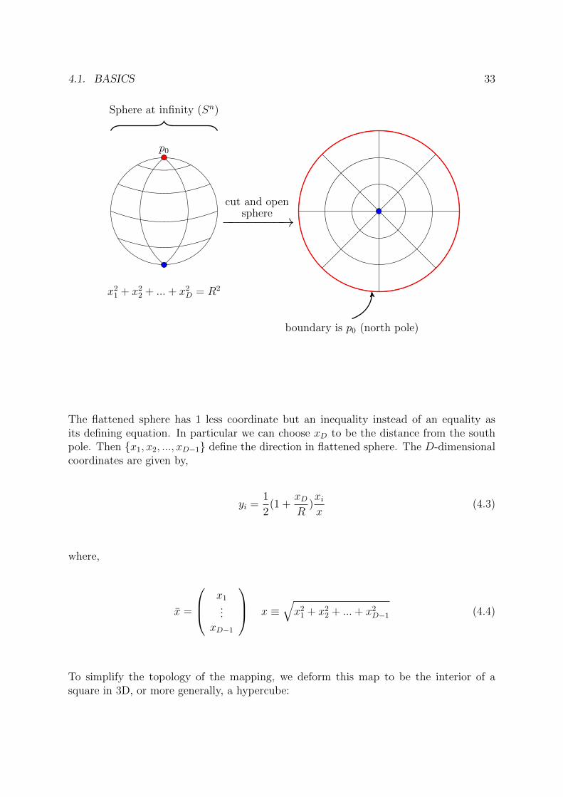
Sphere at infinity (Sn)

x21 + x22 + ...+ x2D = R2

The flattened sphere has 1 less coordinate but an inequality instead of an equality asits defining equation. In particular we can choose xD to be the distance from the southpole. Then x1, x2, ..., xD−1 define the direction in flattened sphere. The D-dimensionalcoordinates are given by,

yi =1

2(1 +

xDR

)xix

(4.3)

where,

x =

x1...

xD−1

x ≡√x21 + x22 + ...+ x2D−1 (4.4)

To simplify the topology of the mapping, we deform this map to be the interior of asquare in 3D, or more generally, a hypercube:

34 CHAPTER 4. HOMOTOPY THEORY

boundary is p0 (north pole)

deformcircle−−−→

In particular we use the coordinates,

zi =1

2

(1 +

r

Myi

)r ≡

√∑i

y2i , i = 1, 2, ..., D − 1 (4.5)

where the zi now denote the distances along each direction in this hypercube. In D = 3(3 spatial dimensions), its the two directions in a square. These are what we will call the“standard coordinates”. A given map can be represented pictorally as,

f(z)

With this machinery we can define group product f = f2 · f1 as

f(z1, z2, ..., zD−1) =

f1(z1, ..., zD−2, 2zD−1) zD−1 ≤ 1/2f2(z1, ..., zD−2, 2zD−1) zD−1 ≥ 1/2

(4.6)

In words: you take two maps and squash them together such that the product map isequal to the first map for zD−1 ≤ 1/2 and the second map for zD−1 ≥ 1/2. The rescalingby a constant of zD−1 shows that the maps are “squashed”. Further, we emphasize thatfor each map p0 is always on the boundary and so the product map still has p0 on theboundary. Pictorally we have,

× =

4.2. IMPORTANT EXAMPLES 35

One can show that we can apply this product to equivalence classes:

[f2] · [f1] = [f2 · f1] (4.7)

i.e., [f2] · [f1] is independent of choice on f2 and f1. Furthermore, one can show thisproduct defines a group, i.e., that it contains an identity element, is associative, and hasan inverse. Furthermore, one can show that n ≥ 2, the group is commutative (abelian).The group is denoted,

πn(M) (4.8)

where for n = D − 1 for the sphere at infinity.

4.2 Important examples

We now present some relevant examples which we will refer back to throughout thesenotes. Consider the mappings from a circle to a 2-sphere order higher dimensional space:

π1(Sm) m ≥ 2 (4.9)

This can be written as a mapping:S1 → Sm (4.10)

Claim 6. The only element in π1(Sm) is the unit element.

Proof. Since Sm is a larger space then S1 there must at least one point in Sm which is notmapped to in S1. Thus we are free to consider the mapping removing this point in Sm.This mapping is homotopically equivalent to a disk (i.e., it can always be continuouslydeformed to a disk) so pictorally:

continuouslydeform

circle at ∞


Any circle will always map to some closed path on the disk. This path can always becontinuously deformed to a point. This is easy to show explicitly for a circular imagepath, charactorized by an angle θ. We denote the point in the image by parameters, xand y. In this case we can consider the homotopy,

F(t, θ) = r0

(t cos θ + (1− t)

t sin θ

)(4.11)

where we have chosen as or base point F(t, 2π) = (r0, 0). For t = 1 this is just a circularpath and for t = 1 this is just a point in the image and this always has the basepoint,x(t, 2π) = r0, y(t, 2π) = 0.

While we only show this explicitly for a circular path its easy to convince yourselfthis will hold for a generic path as long x and y are valid coordinates (i.e., there are notopological defects, e.g., a donut shape where clearly x, y coordinates would not makesense. Thus this mapping is homotopically equivalent to the mapping to a constant andhence π1(Sm) is the unit element.

More generally we have,

Claim 7. For any m > n: πn(Sm) = ∅

We defer proof of this claim to a later lecture once we’ve developed a bit more ma-chinery.

Claim 8. π1(S1) = Z (the homotopy group of the circle at infinity to a circle is the groupintegers under addition).

Proof. Recall that in equation 3.65 we considered this exact mapping:

f : S1 → S1

0 ≤ θ ≤ 2π 0 ≤ σ ≤ 2π(4.12)

We found the mappings, k1θ and k2θ, were homotopically equivalent only if k1 = k2.Therefore, we conclude that the homotopy group is composed of an infinite set of homo-topies charactorized by an integer.

Claim 9. We can generalize the previous relation: πn(Sn) = Z

Proof. We can charactorize the sphere at infinity and the coset sphere by two sets ofangles:

θ = (θ1, θ2, ...) (4.13)

σ = (σ1(θ), σ2(θ), ...) (4.14)

The volume of the domain is given by,

Vdom =

∫Sn

√g(θ)dθ1dθ2...dθn (4.15)

4.2. IMPORTANT EXAMPLES 37

The volume of the range is,

Vran =

∫Sn

√g(σ)dσ1dσ2...dσn (4.16)

=

∫Sn

√g(σ) det

(dσidθj

)dθ1dθ2...dθn (4.17)

where the integral runs over the full range of the sphere, i.e., its an integral including thepotential multiple coverings of the group. The ratio of these volumes will be given by the“covering number” or the number of times the range covers the domain:

k ≡ VranVdom

(4.18)

As we’ve seen the σs form an inequivalent homotopy if they cover the θs a differentnumber of times. Thus, k is an integer.

As an example of the above consider π1(S1) where σ = kθ:

Vdom =

∫ 2π

0

dθ = 2π (4.19)

Vran =

∫ 2πk

0

dσ = k

∫ 2π

0

dθ = 2πk (4.20)

Lets now consider the cases where the image is “smaller” than the sphere at infinity.One can show:

Claim 10. π2(S1) = ∅Proof. The generic mapping from the 2-sphere to the circle with two sections, z > 0 andz < 0:

σ(x, y) (4.21)

where z defined as ±√R2 − x2 − y2. We show that for each half we can shrink the

half-sphere into a point and so we can shrink the whole sphere. Consider the homotopy,

σ(tx+ 1− t, yt) (4.22)

which has the base point, x = 1, y = 0 with the image base point σ(1, 0). Clearly this isa continuous deformation keeping the basepoint fixed. We can trivially do the same forthe z < 0 half and so this mapping is equivalent to the constant mapping:

σ

∣∣∣∣t=0

= σ(1, 0) (4.23)

More generally we have,

Claim 11. πn(S1) = ∅, n > 1

Unlike the lasso’ing a basketball these results are not intuitive. One might expect thelogic we used for π2(S1) to transfer over to π3(S2) however it does not.


4.3 Exact homotopic sequence

4.3.1 Basics

Computing homotopy groups is a difficult task. A very useful tool is called “exact homo-topy sequence. As usual our goal to find a mapping,

M : G1 → G2 (4.24)

Before we introduce the sequences, we need some definitions:

Def. 7. kerM : the set of all elements in G1 that are mapped to the identity element ofG2:

ker(M) = g ∈ G1,M(g1) = 1 (4.25)

Def. 8. ImM : the set of all elements in G2 which are mapped to by something in G1:

ImM = g2 ∈ G2 | ∃g1 ∈ G1,M(g1) = g2 (4.26)

Def. 9. Exact: A given sequence,

G1M1−−→ G2

M2−−→ G2M3−−→ · · · (4.27)

is exact ifImMi = ker(Mi+1) ∀i (4.28)

Claim 12. There exists a sequence,

πn+1(G/H)→ πn(H)M1−−→ πn(G)

M2−−→ πn(G/H)M3−−→ πn−1(H)

M ′1−−→ · · · (4.29)

Proving this claim is feasible but somewhat technical. Instead we take this for grantedand proceed to applications of this theorem.

4.3.2 Examples

Perhaps the simplest application of this is for the sequence:

∅ M1−−→ GM2−−→ ∅ (4.30)

Claim 13. If this is an exact sequence (one where ImM1 = kerM2) then ⇒ G = ∅.

Proof. An ∅ can only map into ∅ and so ImM1 = ∅. Furthermore, by the definition ofthe kernal of M2 (all elements in G which are mapped to the identity, kerM2 = G). Sincewe have an exact sequence we also have, kerM2 = ∅. Therefore, kerM2 = G = ∅

Claim 14. If the sequence,

∅ M1−−→ AM2−−→ B

M3−−→ ∅ (4.31)

is exact then,A = B (4.32)

4.3. EXACT HOMOTOPIC SEQUENCE 39

Proof. Again we have,

ImM1 = ∅ = kerM2 (4.33)

kerM3 = B = ImM2 (4.34)

M2 is a map from A→ B whose kernal is trivial (only identity of A maps to the identityof B) and whose image is B (the set of elements of A which map to B are equal to B).Thus there are no “extra elements” in A and the map is one-to-one and so,

A = B (4.35)

Now lets consider some applications of these ideas into actual groups we will beinterested in.

Claim 15. π3(S2) = Z

Proof. Recall that for the breaking of SU(2) → U(1), the vacuum manifold is equal to a2-sphere: SU(2)/U (1) = S2. Thus we can instead study π3(SU(2)/U(1)). This is muchsimpler since now we can use our exact homotopic sequence. We have,

π3(H) → π3(G) → π3(G/H) → π2(H) (4.36)

or π3(U(1)) → π3(SU(2)) → π3(SU(2)/U(1)) → π2(U(1)) (4.37)

We know that π3(U(1)) = π3(S1) = ∅ and similarly, π2(U(1)) = ∅. Thus we can use thetrick we just learned to say,

π3(SU(2)/U(1)) = π3(SU(2)) (4.38)

since SU(2) = S3, SU(2)/U(1) = S2, and earlier we showed that π3(S3) = Z so,

π3(S2) = Z (4.39)

Claim 16. π1(SO(3)) = Z2

Proof. Consider G = SU(2) and H = Z2 with the sequence,

π1(SU(2))︸︷︷︸∅

→ π1(SU(2)/Z2)→ π0(Z2)→ π0(SU(2))︸︷︷︸∅

(4.40)

π0(G) measures how many connected components G has. Thus π0(Z2) = Z2. Further-more, π1(SU(2)/Z2) = π1(SO(3)). Therefore,

π1(SO(3)) = Z2 (4.41)


Claim 17. π1(SO(N)) = Z2 for N ≥ 3.

Proof. We can again use our Higgs intuition to simplify the problem. For a general SO(N)symmetry broken with a scalar φ, a fundamental of SO(N),

〈φ〉 =

v0...0

(4.42)

After φ gains a VEV, the unbroken subgroup is SO(N − 1) given a coset,

G/H = SO(N)/SO(N − 1) = SN−1 (4.43)

Now consider the exact sequence,

π2(SO(N)/SO(N − 1))︸︷︷︸∅

→ π1(SO(N − 1))→ π1(SO(N))→ π1(SO(N)/SO(N − 1))︸︷︷︸∅

(4.44)where the endpoints are both trivial as long as N ≥ 4. This implies that,

π1(SO(N)) = π1(SO(N − 1)) (4.45)

For N = 4 we have,π1(SO(4)) = π1(SO(3)) = Z2 (4.46)

where we have used our previous result. Applying this relation consecutively we get,

π1(SO(N)) = Z2 N ≥ 3 (4.47)

Claim 18. π1(SU(N)) = ∅ for N ≥ 2

Proof. Again we use our knowledge of spontaneous symmetry breaking to help us extractthe homotopy group. For a fundamental scalar charged under at SU(N) we have,

|φ|2 =

2N︷︸︸︷(φR1 )2 + (φI1)

2 + (φR2 )2 + ... (4.48)

Thus the vacuum manifold is a 2N − 1 sphere:

SU(N)/SU(N − 1) = S2N−1 (4.49)

Now consider the exact sequence,

π2(SU(N)/SU(N − 1))︸︷︷︸∅

→ π1(SU(N − 1))→ π1(SU(N))→ π1(SU(N)/SU(N − 1))︸︷︷︸∅

(4.50)where the end points are the trivial group if N ≥ 2. Thus we have,

π1(SU(N)) = π1(SU(N − 1)) (4.51)

since π1(SU(2)) = ∅ we can iteratively show that π1(SU(N)) = 0 for all N ≥ 2.

4.3. EXACT HOMOTOPIC SEQUENCE 41

One can similarly show two other important homotopy groups:

Claim 19. π2(SU(N)) = ∅

This will be used for studying soliton solutions in 3 + 1 dimensions.

Claim 20. π3(SU(N)) = Z

This will be important when we discuss instantons since instantons in D dimensionsare equivalent to solitons in D − 1 dimensions.

Chapter 5

Magnetic Monopoles

5.1 Monopoles in general

As we’ll see in 3 + 1 dimensions soliton solutions of spontaneously broken gauge theoriesconsist of a tower of monopoles, each with different topological charge. However, beforeapplying our knowledge of topological field theory, let us first discuss the properties ofmonopoles in general.

An electric monopole in electromagnetism is simply a charged particle with charge qwhose E field takes the form,1

E = er

r3(5.1)

One can form an analogue of this for a magnetic monopole with magnetic charge, g,

B = gr

r3(5.2)

5.1.1 Dirac’s derivation

How will such a monopole behave? Dirac’s insight: If we can come up with a find amagnetic field configuration in EM for which there does not exist a test that would dif-ferentiate it from a monopole than that system should share properties with a monopole.

Consider an half-infinite solenoid:

1The prefactor here is of course just conventional, but we attempt to keep gaussian units throughtoutthis discussion.

42

5.1. MONOPOLES IN GENERAL 43

B

...

This is called a Dirac string and has B field lines that look just like a monopole. Theonly difference between the Dirac string and the monopole is the Dirac string has a fluxalong the tube,

Φ =

∫B · da = 4πg

r3

r3= 4πg (5.3)

where we used that the flux in the tube should also be equal to the flux emitted by theend. Is this flux an observable quantity? It can be observed through the Abrahav-Bohmeffect.

Recall that the Schrodinger equation with a magnetic field is given by,

−~2

2m

(∇+

ie

~cA(r)

)2

ψ(r) + V (r)ψ(r) = Eψ(r) (5.4)

If we consider a change of variables,

ψ(r) = exp

(− ie~cf(r)

)ψ0(r) (5.5)

with

f(r) =

∫ r

r0

A(r′) · dr′ ⇒ ∇f(r) = A(r) (5.6)

Then ψ0(r) satisfies, (− ~2

2m∇2 + V

)ψ0(r) = Eψ0(r) (5.7)

Therefore, the presence of A gives an additional position dependent phase to ψ. Thiscan be detected through interference. Consider the following setup:

44 CHAPTER 5. MAGNETIC MONOPOLES

e−source

r+

r−

flux

L

a

where the flux tube represents the center of the Dirac string, far away from the monopole-like end. The magnetic flux modifies the interference pattern due to the additional phase.This phase is independent of path (since A is a conservative vector field), and so the phasedifference of the bottom and top wavefunctions (assuming they start in phase) is,

exp

(1

λ(r+ − r−) +

e

~c

∮A · dr

)(5.8)

where L is the distance from the slits to the screen, λ is the wavelength, and

r± =√L2 + (y ± a/2)2 (5.9)

The first term gives the standard formula for the double slit interference and the secondis the new addition due to the fluxtube. The new term can be written,

e

~c

∮A · dr =

e

~cΦ (5.10)

For this term to be unphysical we must have,

e

~cΦ = 2πn n ∈ Z (5.11)

Using our expression for the flux computed earlier we have,

g =~c2en (5.12)

Thus a Dirac string with quantized charge with quantized charge, shares properties witha monopole. Thus we conclude that a monopole can’t have arbitrarily charged monopolesbut only quanta of ~c/2e.

5.1. MONOPOLES IN GENERAL 45

5.1.2 Derivation using quantization of angular momentum

Now consider an alternative derivation of the same result using angular momentum.Consider an electric monopole at the origin with a magnetic monopole a distance r′

away. For simplicity we place the magnetic monopole along the z direction:

g

r′

r

θ

e

The electromagnetic and magnetic fields of the system are,

E = er

r3B = g

r− r′

|r− r′|3(5.13)

giving an angular momentum,

∫dJ =

1

4πc

∫r×

mom density︷︸︸︷(ε0E×B dV ) (5.14)

= − ge

4πc

∫drr2

∫d cos dφ

r× (r× r′)

r3 |r− r′|3(5.15)

The numerator can be simplified using the triple product identity,

numerator = (r · r′)r− r2r′ (5.16)

= r2r′(cos θr − z) (5.17)

which gives,

J = − ge

4πc

∫dr rr′

∫d cos

∫dφ

(cos θr − z)

(r2 + r′2 − 2rr′ cos θ)3/2(5.18)

Note that since x ∝ sinφ, y ∝ cosφ:∫dφf(r, θ)r = 2πf(r, θ) cos θz (5.19)

and so we can write the above as,

J =ge

2cz

∫dr rr′

∫ 1

−1dcθ

1− c2θ(r2 + r′2 − 2rr′cθ)3/2

(5.20)


The integral is easy done using Mathematica:∫ 1

−1dx

1− x2

(r2 + r′2 − 2rr′x)3/2=

4

3

1r′3

r < r′1r3

r > r′(5.21)

and so,

J =ge

2c

4

3z

[∫ r′

0

drr

r′2+

∫ ∞r′

r′

r2

](5.22)

=ge

cz (5.23)

Since angular momentum is quantized, with a minimum value of ~/2:

g =~c2en (5.24)

in agreement with the result we derived completely independently above.

Both the derivations above required an electric charge to derive the quantizationcondition. We have taken the charge to be electron-like, but we know that we have otherobjects with smaller charges then electrons, quarks. If we consider the derivations abovewith smaller charges, then the lowest magnetic charge must be larger. However, thisconclusion is a bit too quick. If a particle exists, like quarks, that has additional chargesas well as electromagnetic charges the phase from the Aharonov-Bohm effect (or angularmomentum in the second derivation) can be at least partially cancelled canelled by phasesdue to additional interactions. For example we can find the phase in the Aharonov-Bohmeffect using a “down-quark Dirac string“ is,

exp[−i( e

3~c− gs

~c

)](5.25)

where the sign is due to color being attractive. This type of cancellation occurs for GUTmonopoles.

5.2 Dyons

Above we considered particles with only electric or only magnetic charge. Dyons are(hypothetical) particles that carry both charges. What is there quantization condition?Consider two such particles with charges,

(q1, g1) (q2, g2) (5.26)

Now consider particle one going around particle two,

5.3. DUALITY TRANSFORMATION OF MAXWELL’S EQUATIONS 47

2

1

The phase of −4πiq1g2/~c and 4πiq2g1~c respectively giving a relative phase shift of,

exp

[−i4π

~c(q1g2 − q2g1)

]. (5.27)

This phase shift is unobservable if,

q1g2 − q2g1 =1

~cn

2(5.28)

This is known as the Schwinger-Dyson quantization condition. For q1 = e, q2 = 0, g1 = 0,g2 = g we recover the earlier result. However, for dyons electric charges are not all integermultiples of a fundamental charge. In particle consider two particle with charges,

1

~c

(n1 −

θ

2πm1,m1

),

1

~c

(n2 −

θ

2πm2,m2

)(5.29)

for n1, n2,m1,m2 ∈ Z. The Dirac quantization condition gives,

q1g2 − q2g1 =1

~c(n1m2 − n2m1) (5.30)

(the θ term cancels) satisfying the quantization condition. Hence there is a continuos setof charges parameterized by a parameter θ that can exist. The Witten effect [4] showsthat this parameter is equal to the θ angle of the gauge theory.

5.3 Duality transformation of Maxwell’s equations

Maxwell’s equations are given in their differential form as,

∇ · E = 4πρe (5.31)

∇ ·B = 0 (5.32)

∇× E = −1

c∂tB (5.33)

∇×B =1

c∂tE +

4π

cje (5.34)


where ρe and je are the electric charge and current respectively. Generically there is nosymmetry relating the E and B fields. However, when the sources vanish, ρe, je = 0 theequations are symmetric under an SO(2) transformation:(

EB

)→(

cθ sθ−sθ cθ

)(EB

)(5.35)

This is known as the duality transformation of Maxwell’s equations. Now suppose wehad electric and/or magnetic charges. You can always redefine your fields by rotatingaway one of the charges using a duality transformation:

(q, g)→ (qcθ + gsθ,−qsθ + gcθ) (5.36)

Thus there is nothing special about magnetism. The statement that “magnetic chargesdon’t carry charges” is a statement that we can always define our electric and magneticfields such that the “one that has a source” is the electric field and the other one is themagnetic field.

How would Maxwell’s equation look like with a magnetic source? To see this considerthe simplest electromagnetic duality, α = 90o. In this case,

E→ B B→ −E (5.37)

Recall that Maxwell’s equation can be written in terms of the field strength tensor,

∂µFµν =4π

cje,ν ∂νF

µν = 0 (5.38)

where Fαβ ≡ εαβµνFµν . In matrix form,

F =

0 ET

0 Bz −By

−E −Bz 0 Bx

By −Bx 0

F =

0 −BT

0 Ez −EyB −Ez 0 Ex

Ey −Ex 0

(5.39)

Thus under such a rotation we have, F → −F and F → F . Adding in magnetic chargeswe expect,

∂µFµν =4π

cjeν ∂µFµν =

4π

cjmν (5.40)

We will show that the topological current in monopole-type soolitons will endeed enterin jmµ .

5.4 Topological Monopoles

Thus far we have studied generic properties of monopoles. We now consider a particleexample.

5.4. TOPOLOGICAL MONOPOLES 49

5.4.1 ’t Hooft-Polyakov monopole

Consider the Georgi-Glashow model of an SO(3) symmetry with a triplet φa and poten-tial,

U(φ) = λ(φ2 − v2)2 (5.41)

The symmetry breaking pattern is,

SU(2)→ U(1) (5.42)

Thus we have two broken generators (in the toy SM, these would give mass to the W±

with mass mW = ev). The relevant homotopy group is,

π2(SU(2)/U(1)) = π2(S2) = Z (5.43)

Thus we expect a conserved integer charge. What is the conserved current? We won’tderive the form of the current but instead reveal the answer and then show that it isindeed conserved. The desired current is,

Kµ =1

8πεµνρσεabc(∂

νφa)(∂ρφb)(∂σφc) (5.44)

where φa ≡ φa/v. This is clearly conserved since,

∂µKµ ∝ εµνρσ(∂µ∂νφa)(...) + ... = 0 (5.45)

Note that this current is a non-Noether current, but of topological origin. The conservedcharge is,

Q =

∫d3xK0 (5.46)

=1

8πεabc

∫d3x

(φ1φa∂2φb∂3φc − ∂2φa∂1φb∂3φc + ...

)(5.47)

=1

8πεabcεijk

∫d3x∂iφa∂jφb∂kφc (5.48)

=1

8πεabcεijk

∫d3x∂i

[φa∂jφb∂kφc

]−(((((((((((φa(∂i∂jφb)∂kφc + ... (5.49)

=1

8πεabcεijk

∫d3x∂i

[φa∂jφb∂kφc

](5.50)

To simplify this integral note that,∫dDx∂if(x) =

∫dΩ lim

r→∞

xirf(x) (5.51)

which can be derived as a particular case of Gausses law by considering a sphericalintegration region. Furthermore,

dΩ =1

(D − 1)!dθ1dθ2...

1

rD−1

[r

x1det

∂x

∂θ 1− r

x2det

∂x

∂θ 2+ ...

](5.52)

=1

(D − 1)!dθ1dθ2...

1

rD−1εim1m2...εp1p2...

r

xi

(∂xm1

∂θp1

∂xm2

∂θp2...

)(5.53)


or for D = 3:

dΩ =1

2dα1dα2εimnεpq

r

xi

∂xm∂αp

∂xn∂αq

(5.54)

where α1 and α2 are the angles (usually denoted θ and φ). Thus we conclude,∫d3x∂if(x) = εimnεpq

1

2d2α lim

r→∞

∂xm∂αp

∂xn∂αq

f(α) (5.55)

and

Q =1

16πεabcεijkεimnεpq

∫d2α lim

r→∞φa∂φb

∂αw

∂φc

∂αv

∂αw∂xj

∂αv∂xk

∂xm∂αp

∂xn∂αq

(5.56)

=1

16π

∫d2αεabcεpqφ

a

(∂φb

∂αp

∂φc

∂αq− ∂φb

∂αq

∂φc

∂αp

)(5.57)

=1

8π

∫d2αεabcεpqφ

a ∂φb

∂αp

∂φc

∂αq(5.58)

Now convert the integral to coordinates in the internal φa space, (ξ1, ξ2) which gives,

Q =1

4π

∫d2ξ

1

2εabcεrs

∂φb

∂ξr

∂φc

∂ξsφa (5.59)

The factor in the center is just the differential of the surface in the internal space and sowe can write,

Q =1

4π

∫dV int∂aφ

a (5.60)

where the volume integral now runs over the internal (image) space.We want to argue that this topological current will play the role of the magnetic

current. For these topological solutions the VEV is not pointing in the smae directionall the time. This implies that the unbroken U(1) direction is changing. Given this howshould you define Fµν?

’t Hooft showed that,

FEMµν = φaF a

µν −1

eεabcφaDµφ

bDνφc (5.61)

is gauge invariant. Note that if φ = (0 , 0 , 1)T then DµφaD2

νφ = 0 and so FEMµν = F 3

µν .

Far out since Dµφ contributes to the energy density we have,

Dµφ→ 0 ⇒ FEMµν ' φaF a

µν (5.62)

With lots of algebra one can show that,

1

2εµνρσ∂

νF ρσEM =

4π

eKµ (5.63)

Bibliography

[1] S. Coleman. Aspects of Symmetry: Selected Erice Lectures. Cambridge UniversityPress, 1988.

[2] R. Rajaraman. Solitons and instantons : an introduction to solitons and instantonsin quantum field theory / R. Rajaraman. North-Holland Pub. Co. ; sole distributorsfor the USA and Canada, Elsevier Science Pub. Co Amsterdam ; New York : NewYork, N.Y, 1982.

[3] A. I. Vainshtein, V. I. Zakharov, V. A. Novikov, and M. A. Shifman. ABC’s ofInstantons. Sov. Phys. Usp., 25:195, 1982. [Usp. Fiz. Nauk136,553(1982)].

[4] E. Witten. Dyons of charge e/2. Physics Letters B, 86(3):283 – 287, 1979.

51

Solitons and Instantons LECTURE NOTES - Cornell...

Documents

Transcript of Solitons and Instantons LECTURE NOTES - Cornell...