J . Fluid Mech. (1990), vol. 216, p p . 323-342 Printed in Great Britain

323

Solidification of an alloy cooled from above Part 1. Equilibrium growth

By ROSS C. KERR't, ANDREW W. M. GRAE WORSTER'S A N D HERBERT E. HUPPERT'.2

Department of Applied Mathematics and Theoretical Physics, Institute of Theoretical Geophysics,

University of Cambridge, Silver Street, Cambridge CB3 9EW, UK

(Received 22 June 1989)

The interaction between the solidification and convection that occurs when a melt is cooled from above is investigated in a series of three papers. In these papers we consider a two-component melt that partially solidifies to leave a buoyant residual fluid. The solid forms a mushy layer of dendritic crystals, the interstices of which accommodate the residual fluid. The heat extraction through the upper boundary, necessary to promote solidification, drives convection a t high Rayleigh numbers in the melt below the mushy layer. The convection enhances the heat transfer from the melt and alters the rate of solidification. In this paper the various phenomena are studied in a series of laboratory experiments in which ice is frozen from aqueous solutions of isopropanol. The experiments are complemented by the development of a general theoretical model in which the mush is treated as a continuum phase with thermodynamic properties that are functions of the local solid fraction. The model, which is based upon principles of equilibrium thermodynamics and local conservation of heat and solute, produces results in good agreement with the experimental data. Careful comparisons between this theory and experiments suggest the need to explore non-equilibrium effects, which are investigated in Parts 2 and 3.

1. Introduction Fluid convection in a cooled melt significantly influences the resulting solidi-

fication. The fluid motions affect heat and mass transfer rates that ultimately determine compositional variations and crystal habit within the solidified product. The interactions between solidification and convection are of particular importance in the casting of metal alloys, the production of semiconductor crystals and the formation of igneous rocks.

Fluid motions in the melt can occur naturally when solidification takes place in a gravitational field ; the cooling necessary for solidification causes temperature gradients that can lead to thermal convection. Additionally, when an alloy is solidified, compositional gradients arise as one component is preferentially incorporated into the growing solid, and these too can cause convection. Huppert & Worster (1985) identified six different regimes in systems cooled from a single

t Present address : Research School of Earth Sciences, ANU, GPO Box 4, Canberra, ACT 2601, Australia.

3 Present address : Departments of Engineering Sciences and Applied Mathematics, and Chemical Engineering, Northwestern University, Evanston, IL 60208, USA.

324 R. C. Kerr, A . W. Woods, M . G. Worster and H . E . Huppert

horizontal boundary that forms either the upper or lower boundary of the melt. The type of convection that can occur depends both on the applied thermal field and on whether the residual fluid (depleted of the component forming the solid phase) has a greater, a lesser, or the same density as the original melt. Huppert & Worster then analysed a system with a dense residual which is cooled from below. In such a case, convective motions are absent because both the thermal and compositional fields are gravitationally stable.

The freezing temperature of an alloy (its liquidus temperature) is a function of its composition. The minimum freezing temperature, below which the alloy is completely solid, is called the eutectic temperature. In this paper we only consider cases in which the cooled boundary has a temperature above the eutectic temperature and so the system will always be only partially solidified.

A feature of special interest in alloy solidification is the formation of partially solidified regions called ‘mushy layers’, which were discussed in some detail by Worster (1986). A mushy layer is a region of mixed phase comprising a matrix of solid, dendritic crystals with fluid-filled interstices. It forms as a result of local supersaturation (temperature below the local liquidus temperature) in the melt, which commonly occurs during the solidification of alloys owing to the much slower diffusion rate of most solutes compared with that of heat. By increasing the surface area a t which solidification can take place, the mushy layer enhances the release of both latent heat and rejected fluid. This simultaneously raises the local temperature and depresses the local liquidus temperature so that the supersaturation is reduced and may be almost eliminated. Since rejected fluid is accommodated within the interstices of the mush, the rate of growth of the mushy layer is controlled principally by the rate of heat transfer.

In’this series of papers, summarized in Kerr et al. (1989), we consider the case of a two-component alloy cooled from above which rejects a buoyant residual fluid. The system is therefore unstable to thermal convection while the compositional field is stabilizing. Turner, Huppert & Sparks (1986, herein referred to as THS) described a number of laboratory experiments in such a geometry and also presented a theoretical analysis of the simpler system in which a pure (or eutectic) melt is cooled and solidified from above. Their theory elucidated the changing balances between heat conduction through the solid, the latent heat released by the solidification of the melt and the heat transfer from the convecting fluid below. In considering the solidification of an alloy, we have additionally to concern ourselves with the evolution of a mushy layer.

In $2 we describe a set of carefully controlled laboratory experiments designed to provide accurate data on the solidification of an alloy cooled from above. In these experiments, ice was frozen from a mixture of water and isopropanol. The experimental data are used to test the accuracy of a mathematical model, which we formulate in $ 3 and discuss in $4. The model employs partial differential equations to describe heat and solute conservation within the mushy layer, which is treated as a new continuum phase assumed to be in local thermodynamic equilibrium. The convective heat flux from the liquid region is calculated with a semi-empirical formula appropriate for convection a t high Rayleigh numbers. The model is closed by the hypothesis of marginal equilibrium at the growing interface between the mushy layer and the liquid, which was introduced by Worster (1986).

Global conservation relationships for heat and solute are derived from the full system of differential equations in the Appendix. The resulting set of ordinary differential equations, which extends the model of Huppert & Worster (1985), is

Solidi$cation of a n alloy cooled from above. Part 1 325

much easier to compute than the local model. It can produce good approximate results for some of the gross features of the system, such as the rate of growth of the mushy layer, and may be useful for many practical applications.

2. Laboratory experiments with isopropanol We performed a series of experiments in which aqueous solutions of isopropanol

were cooled from above. The behaviour of many binary melts will be similar to that observed in this particular system, which we chose for a number of reasons. First, the solution satisfied the requirement that when it is cooled, the formation of ice rejects a buoyant alcohol-enriched solution, Second, this system has the convenient feature that the solid (ice) is also less dense than the initial solution, so that, unlike previous experiments (such as those of Chen & Turner 1980; and THS), the experiment is not complicated by small crystals occasionally falling through the solution. Third, reliable thermodynamic data are available for this chemical system. This is essential in order to make comparisons between the experimental and theoretical results. Fourth, the anomalous density maximum a t 4 "C associated with pure water can be eliminated by using a sufficient concentration of isopropanol (greater than about 12 wt %) without the liquidus temperature of the solution becoming inconveniently low. For the experiments described in this paper we used a solution of 16.8 wt YO isopropanol, which has a liquidus temperature of -6.2 "C.

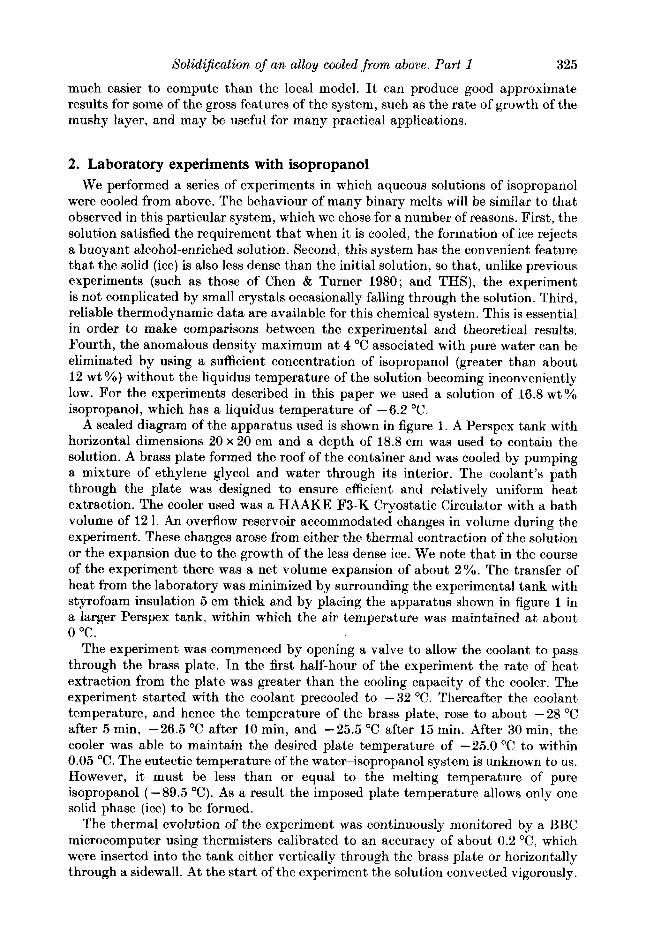
A scaled diagram of the apparatus used is shown in figure 1. A Perspex tank with horizontal dimensions 20 x 20 cm and a depth of 18.8 cm was used to contain the solution. A brass plate formed the roof of the container and was cooled by pumping a mixture of ethylene glycol and water through its interior. The coolant's path through the plate was designed to ensure efficient and relatively uniform heat extraction. The cooler used was a HAAKE F3-K Cryostatic Circulator with a bath volume of 12 1. An overflow reservoir accommodated changes in volume during the experiment. These changes arose from either the thermal contraction of the solution or the expansion due to the growth of the less dense ice. We note that in the course of the experiment there was a net volume expansion of about 2 %. The transfer of heat from the laboratory was minimized by surrounding the experimental tank with Styrofoam insulation 5 cm thick and by placing the apparatus shown in figure 1 in a larger Perspex tank, within which the air temperature was maintained at about 0 "C.

The experiment was commenced by opening a valve to allow the coolant to pass through the brass plate. I n the first half-hour of the experiment the rate of heat extraction from the plate was greater than the cooling capacity of the cooler. The experiment started with the coolant precooled to -32 "C. Thereafter the coolant temperature, and hence the temperature of the brass plate, rose to about -28 "C after 5 min, -26.5 "C after 10 min, and -25.5 "C after 15 min. After 30 min, the cooler was able to maintain the desired plate temperature of -25.0 "C to within 0.05 "C. The eutectic temperature of the water-isopropanol system is unknown to us. However, i t must be less than or equal to the melting temperature of pure isopropanol (-89.5 "C). As a result the imposed plate temperature allows only one solid phase (ice) to be formed.

The thermal evolution of the experiment was continuously monitored by a BBC microcomputer using thermisters calibrated to an accuracy of about 0.2 "C, which were inserted into the tank either vertically through the brass plate or horizontally through a sidewall. At the start of the experiment the solution convected vigorously.

326 R. C. Kerr, A . W. Woods, M . G. Worster and H . E . Huppert

To cooler

- * I 20 cm l o - 10 cm I 1 Scale

FIGURE 1. A scaled diagram of the experimental apparatus.

This convection diminished as the solution temperature decreased from an initial value of 4.0OC: to a constant value of about half a degree below the liquidus temperature (-6.2 "C) after about 400 min.

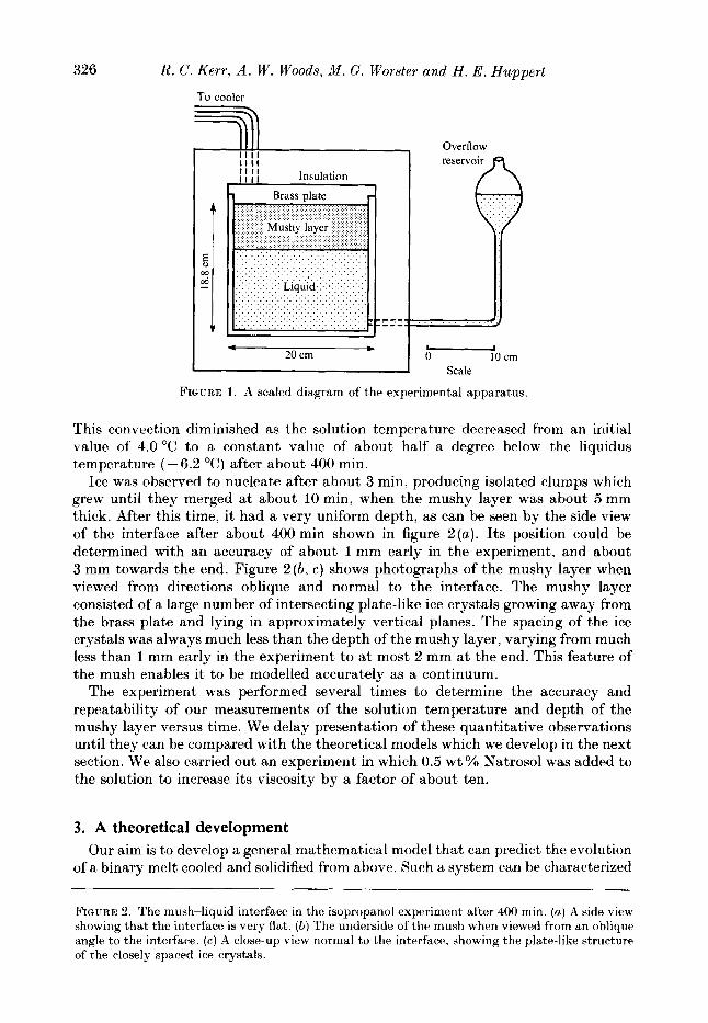
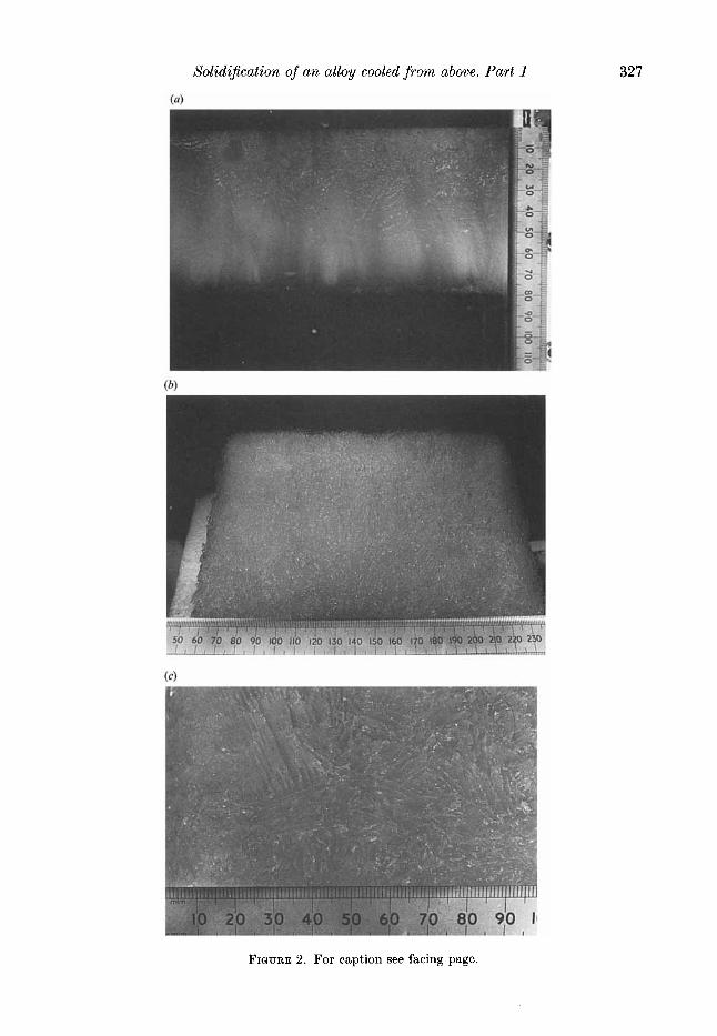
Ice was observed to nucleate after about 3 min, producing isolated clumps which grew until they merged a t about 10 min, when the mushy layer was about 5 mm thick. After this time, it had a very uniform depth, as can be seen by the side view of the interface after about 400 min shown in figure 2(a ) . I ts position could be determined with an accuracy of about 1 mm early in the experiment, and about 3 mm towards the end. Figure 2 ( b , c ) shows photographs of the mushy layer when viewed from directions oblique and normal to the interface. The mushy layer consisted of a large number of intersecting plate-like ice crystals growing away from the brass plate and lying in approximately vertical planes. The spacing of the ice crystals was always much less than the depth of the mushy layer, varying from much less than 1 mm early in the experiment to a t most 2 mm at the end. This feature of the mush enables it to be modelled accurately as a continuum.

The experiment was performed several times to determine the accuracy and repeatability of our measurements of the solution temperature and depth of the mushy layer versus time. We delay presentation of these quantitative observations until they can be compared with the theoretical models which we develop in the next section. We also carried out an experiment in which 0.5 wt % Natrosol was added to the solution to increase its viscosity by a factor of about ten.

3. A theoretical development Our aim is to develop a general mathematical model that can predict the evolution

of a binary melt cooled and solidified from above. Such a system can be characterized

FIGURE 2. The mush-liquid interface in the isopropanol experiment after 400 min. (a) A side view showing tha t the interface is very flat. ( b ) The underside of the mush when viewed from an oblique angle to the interface. ( c ) A close-up view normal to the interface, showing the plate-like structure of the closely spaced ice crystals.

Solidi$cation of an alloy cooled from above. Part 1 327

FIGURE 2. For caption see facing page.

328 R. C. Kerr, A . W. Woods, M . G . Worster and H . E . Huppert

........... \r ............ ;B ............ \,v-.. .......... 4 - 6; - 4-

+! !d ............ 1 1 ............. 1 1 ............. , , .............

+ I I + I ,

+! !+ I .

I ,

............ : 1 : ............... :I; .............. ; I : ............. i i . . \ I \ I

\ I \ I

\ I Y , I \ I

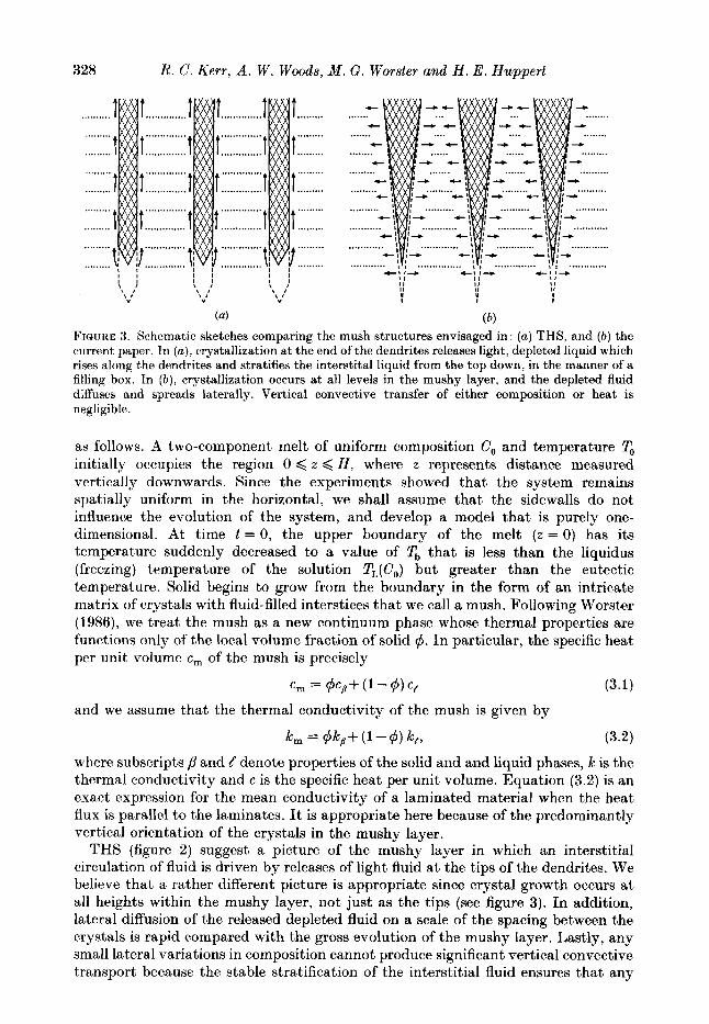
(4 (4 FIGURE 3. Schematic sketches comparing the mush structures envisaged in: (a) THS, and ( b ) the current paper. In (a), crystallization a t the end of the dendrites releases light, depleted liquid which rises along the dendrites and stratifies the interstital liquid from the top down, in the manner of a filling box. In ( b ) , crystallization occurs at all levels in the mushy layer, and the depleted fluid diffuses and spreads laterally. Vertical convective transfer of either composition or heat is negligible.

as follows. A two-component melt of uniform composition C, and temperature T, initially occupies the region 0 < z < H , where z represents distance measured vertically downwards. Since the experiments showed that the system remains spatially uniform in the horizontal, we shall assume that the sidewalls do not influence the evolution of the system, and develop a model that is purely one- dimensional. At time t = 0, the upper boundary of the melt ( z = 0) has its temperature suddenly decreased to a value of Tb that is less than the liquidus (freezing) temperature of the solution TL(Co) but greater than the eutectic temperature. Solid begins to grow from the boundary in the form of an intricate matrix of crystals with fluid-filled interstices that we call a mush. Following Worster (1986), we treat the mush as a new continuum phase whose thermal properties are functions only of the local volume fraction of solid 4. I n particular, the specific heat per unit volume c, of the mush is precisely

c , = 4c,+ (1 - 4 ) c,

k, = 4ks+ (1 -4 ) k,,

(3.1)

(3.2)

and we assume that the thermal conductivity of the mush is given by

where subscripts p and / denote properties of the solid and and liquid phases, k is the thermal conductivity and c is the specific heat per unit volume. Equation (3.2) is an exact expression for the mean conductivity of a laminated material when the heat flux is parallel to the laminates. It is appropriate here because of the predominantly vertical orientation of the crystals in the mushy layer.

THS (figure 2) suggest a picture of the mushy layer in which an interstitial circulation of fluid is driven by releases of light fluid a t the tips of the dendrites. We believe that a rather different picture is appropriate since crystal growth occurs a t all heights within the mushy layer, not just as the tips (see figure 3). In addition, lateral diffusion of the released depleted fluid on a scale of the spacing between the crystals is rapid compared with the gross evolution of the mushy layer. Lastly, any small lateral variations in composition cannot produce significant vertical convective transport because the stable stratification of the interstitial fluid ensures that any

Solidification of an

(4

alloy cooled from above. Part 1

(b)

t I---' I

329

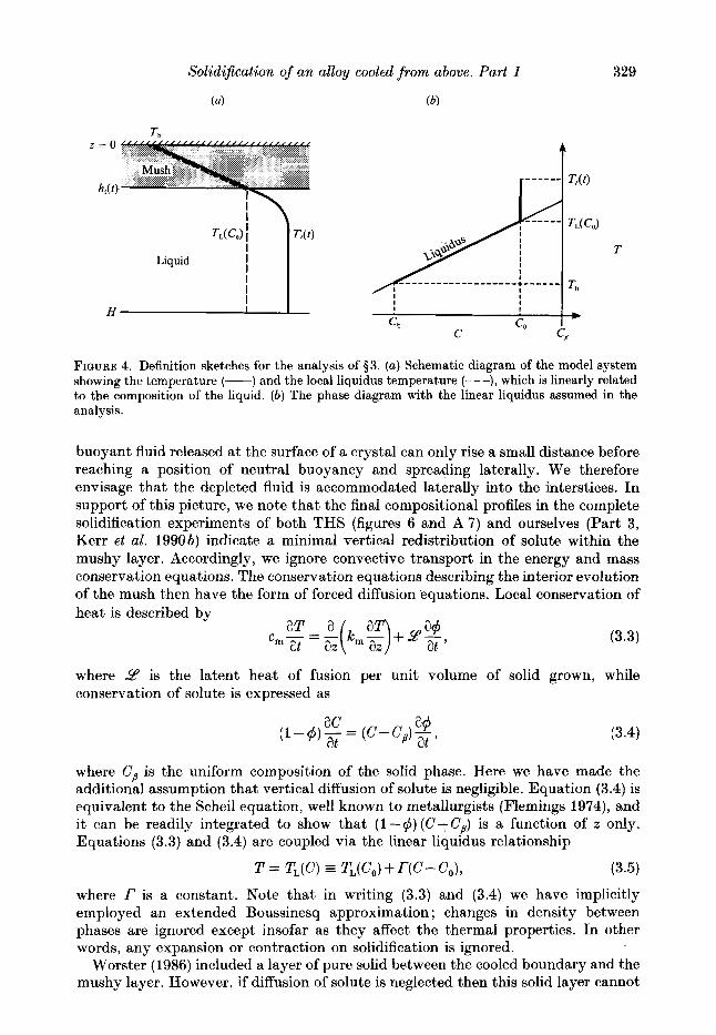
FIGURE 4. Definition sketches for the analysis of $3. (a) Schematic diagram of the model system showing the temperature (-) and the local liquidus temperature (---), which is linearly related to the composition of the liquid. (b ) The phase diagram with the linear liquidus assumed in the analysis.

buoyant fluid released at the surface of a crystal can only rise a small distance before reaching a position of neutral buoyancy and spreading laterally. We therefore envisage that the depleted fluid is accommodated laterally into the interstices. In support of this picture, we note that the final compositional profiles in the complete solidification experiments of both THS (figures 6 and A 7) and ourselves (Part 3, Kerr et al. 1990b) indicate a minimal vertical redistribution of solute within the mushy layer. Accordingly, we ignore convective transport in the energy and mass conservation equations. The conservation equations describing the interior evolution of the mush then have the form of forced diffusion equations. Local conservation of heat is described by

(3.3)

where 2' is the latent heat of fusion per unit volume of solid grown, while conservation of solute is expressed as

ac at

(1-4)- = (3.4)

where Cp is the uniform composition of the solid phase. Here we have made the additional assumption that vertical diffusion of solute is negligible. Equation (3.4) is equivalent to the Scheil equation, well known to metallurgists (Flemings 1974), and it can be readily integrated to show that (1 -$) (C-Ca) is a function of z only. Equations (3.3) and (3.4) are coupled via the linear liquidus relationship

T = TL(C) TL(Co)+r(C-Co), (3.5)

where f is a constant. Note that in writing (3.3) and (3.4) we have implicitly employed an extended Boussinesq approximation ; changes in density between phases are ignored except insofar as they affect the thermal properties. In other words, any expansion or contraction on solidification is ignored.

Worster (1986) included a layer of pure solid between the cooled boundary and the mushy layer. However, if diffusion of solute is neglected then this solid layer cannot

330 R. C. Kerr , A . W . Woods, M . C. Worster and H . E. Huppert

form and the mushy layer extends all the way to the boundary. The typical situation, part way through the evolution of the system, is shown schematically in figure 4. Mush extends from z = 0 to x = h,(t), a t which level the temperature is Ti and the composition of the interstitial fluid is Ci. I n the region hi < z < H , liquid is convecting vigorously and we assume therefore that it well mixed with temperature

and composition C,. At the interface z = h, between mush and liquid, conservation of heat requires that

where FT is the convective heat flux transferred from the liquid to the mush regions. This equation, together with (3.9) below, formed the basis of a model presented by THS for the growth of eutectic solid (rather than mush) from the upper boundary. The first term of (3.6) represents the specific heat needed to accommodate the increase in temperature across the thermal boundary layer as the solid grows. This term, which has been incorporated in the model to conserve heat, was omitted from the analysis presented by THS. Its influence is small whenever a Stefan number based on the temperature drop across the boundary layer, LYpIc,(%-q), is large, which is often the case.

The other boundary conditions that we apply at the interface are a condition of conservation of solute and, in this paper, the condition of marginal equilibrium introduced by Worster (1986). The condition of marginal equilibrium states that the temperature gradient in the liquid ahead of the interface is equal to the gradient of the local liquidus temperature. I n the limit of zero solutal diffusivity the two conditions combine to give

q5 = 0, ci = c, ( z = hi). (3.7)

To estimate the heat transfer across the mush-liquid interface, we note that in our experiments the Rayleigh number Ra associated with the convecting liquid is large (about lo9 a t the start), and thus we adopt the approximate relationship Nu cc Rat, where Nu is the Nusselt number (Turner 1979; Denton & Wood 1979). The dimensional heat flux is therefore taken to be

where g is the acceleration due to gravity, u the coefficient of thermal expansion, K[

and v the thermal diffusivity and kinematic viscosity of the liquid respectively and A is a constant. I n the limit D / K , --f 0, where D is the compositional diffusivity, all the compositional variation is accommodated within the mushy layer and hence the thermal convection in the melt ahead of the mush-liquid interface is unaffected by any compositional buoyancy. Finally, the bulk temperature of the liquid region evolves according to

(3.9)

and we assume that there is no flux of solute across the mush-liquid interface, so that

The governing equations for the whole system can be made dimensionless by c, = c,.

Solidi,fication of an alloy cooled from above. Part 1 33 1

scaling lengths with H , time with H ' / K ~ , temperatures with AT = TL(CO)-q and

(3.10)

Equations (3.3)-(3.5) can then be combined to give the single dimensionless equation

k where k @ + ( 1 - $ ) ,

kC

C S

CC c = q Q + ( l - $ ) + 3 ( l - $ ) 2

- e and 9=-*

The 1 imensionless parameters appearing in (3.13) and (3.1, the mushy layer

9 S = - cc AT '

c -c, and w = B . Q, - Cb

(3.11)

(3.12)

(3.13)

(3.14)

) are a Stefan number for

(3.15)

(3.16)

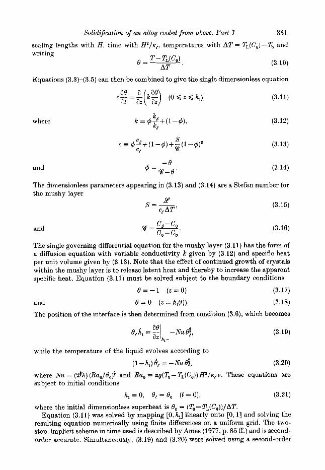
The single governing differential equation for the mushy layer (3.11) has the form of a diffusion equation with variable conductivity k given by (3.12) and specific heat per unit volume given by (3.13). Note that the effect of continued growth of crystals within the mushy layer is to release latent heat and thereby to increase the apparent specific heat. Equation (3.11) must be solved subject to the boundary conditions

8 = - 1 ( z = O ) (3.17)

and e = o (2 = hip)). (3.18)

The position of the interface is then determined from condition (3.6), which becomes

(3.19)

while the temperature of the liquid evolves according to

p h i ) & = -Nut$, (3.20)

where Nu = (&A) (Ra,/8,); and Ra, = ag(T,- TL(Co)) H 3 / q u. These equations are subject to initial conditions

hi = 0, ec = e, ( t = o), (3.21)

where the initial dimensionless superheat is 8, = (T, - T,(C,))/AT. Equation (3.11) was solved by mapping [0, hi] linearly onto [0,1] and solving the

resulting equation numerically using finite differences on a uniform grid. The two- step, implicit scheme in time used is described by Ames (1977, p. 85 ff.) and is second- order accurate. Simultaneously, (3.19) and (3.20f were solved using a second-order

332 R. C. Kerr, A . W . Woods, M . G. Worster and H . E. Huppert

X X

X

-

-

-

* ' I

40 60 80 I

Value

1.832 J cm-3 O C - '

3.912 J ~ m - ~ O C - l

0.022 W cm-' O C - l

0.0037 W cm-I OC-' 306 J ~ 1 3 1 ~ ~

0.057 cm2 s-l 0.056

A

- 0

-10

T ("C)

-20

-30

100

Source

E D B, n C D

A -

-

-

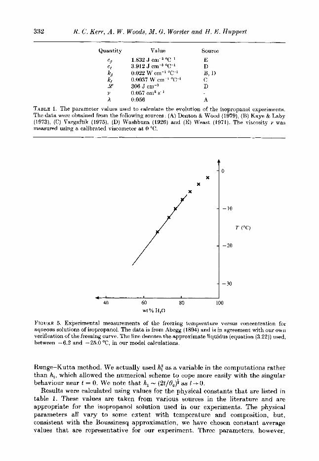
TABLE 1. The parameter values used to calculate the evolution of the isopropanol experiments. The data were obtained from the following sources: (A) Denton & Wood (1979), (B) Kaye & Laby (1973), (C) Vargaftik (1975), (D) Washburn (1926) and (E) Weast (1971). The viscosity v was measured using a calibrated viscorneter at 0 O C .

-10

T ("C)

-20

X X lo

1 - 3 0 - ~-

40 60 80 100 wt Yo H,O

FIGURE 5. Experimental measurements of the freezing temperature versus concentration for aqueous solutions of isopropanol. The data is from Abegg (1894) and is in agreement with our own verification of the freezing curve. The line denotes the approximate liquidus (equation (3.22)) used, between -6.2 and -25.0 "C. in our model calculations.

Runge-Kutta method. We actually used ht as a variable in the computations rather than hi, which allowed the numerical scheme to cope more easily with the singular behaviour near t = 0. We note that hi - (2t/O,$ as t + O .

Results were calculated using values for the physical constants that are listed in table 1. These values are taken from various sources in the literature and are appropriate for the isopropanol solution used in our experiments. The physical parameters all vary to some extent with temperature and composition, but, consistent with the Boussinesq approximation, we have chosen constant average values that are representative for our experiment. Three parameters, however,

Solidi$cation of an alloy cooled from above. Part 1

3

a (10-4 o c - 1 )

2

1

333

I I I I

-12 -8 -4 0 4 8

T ("C)

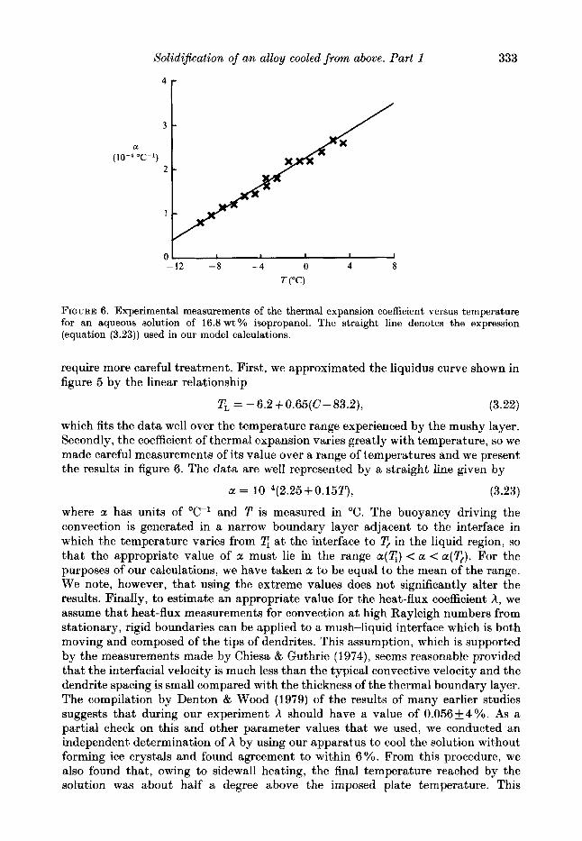
FIGURE 6. Experimental measurements of the thermal expansion coefficient versus temperature for an aqueous solution of 16.8 wt Yo isopropanol. The straight line denotes the expression (equation (3.23)) used in our model calculations.

require more careful treatment. First, we approximated the liquidus curve shown in figure 5 by the linear relationship

TL = -6.2+0.65(C-83.2), (3.22)

which fits the data well over the temperature range experienced by the mushy layer. Secondly, the coefficient of thermal expansion varies greatly with temperature, so we made careful measurements of its value over a range of temperatures and we present the results in figure 6. The data are well represented by a straight line given by

a = 10-4(2.25+0.15T), (3.23)

where a has units of O C - l and T is measured in "C. The buoyancy driving the convection is generated in a narrow boundary layer adjacent to the interface in which the temperature varies from in the liquid region, so that the appropriate value of a must lie in the range a ( q ) < a < a(%). For the purposes of our calculations, we have taken a to be equal to the mean of the range. We note, however, that using the extreme values does not significantly alter the results. Finally, to estimate an appropriate value for the heat-flux coefficient A, we assume that heat-flux measurements for convection a t high Rayleigh numbers from stationary, rigid boundaries can be applied to a mush-liquid interface which is both moving and composed of the tips of dendrites. This assumption, which is supported by the measurements made by Chiesa & Guthrie (1974), seems reasonable provided that the interfacial velocity is much less than the typical convective velocity and the dendrite spacing is small compared with the thickness of the thermal boundary layer. The compilation by Denton & Wood (1979) of the results of many earlier studies suggests that during our experiment h should have a value of 0.056+4%. As a partial check on this and other parameter values that we used, we conducted an independent determination of h by using our apparatus to cool the solution without forming ice crystals and found agreement to within 6%. From this procedure, we also found that, owing to sidewall heating, the final temperature reached by the solution was about half a degree above the imposed plate temperature. This

a t the interface to

334 R. C. Kerr, A . W . Woods, M . G . Worster and H . E. Huppert

0 400 800 I200 I600

t (min)

I I I

I I I I 0 200 400 600 800

t (min)

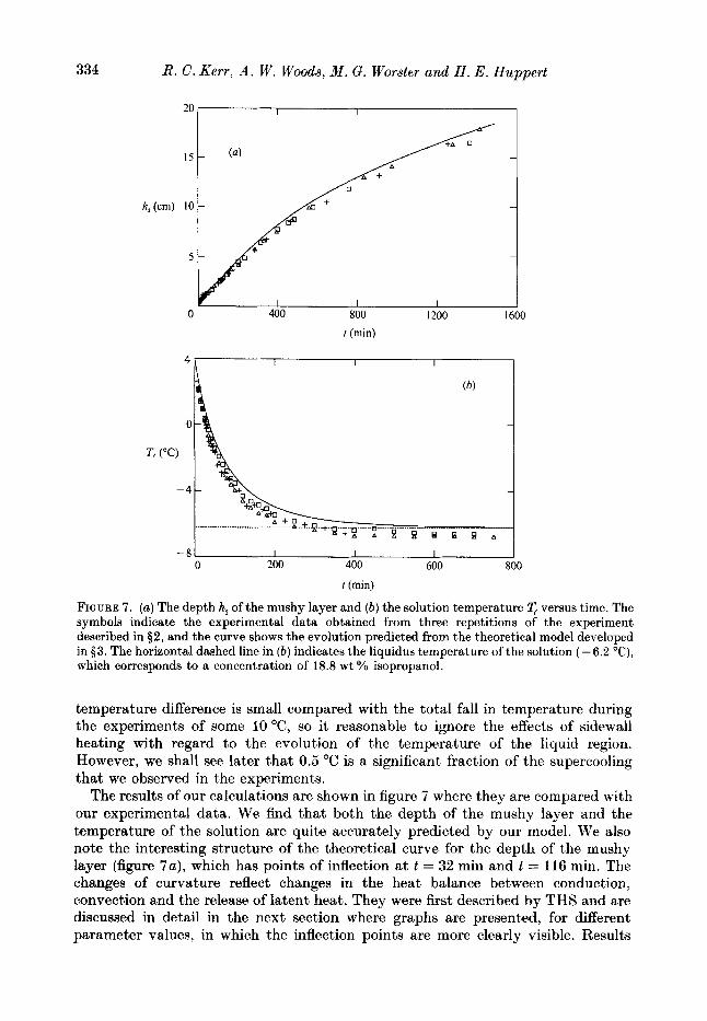
FIGURE 7. (a) The depth hi of the mushy layer and (b ) the solution temperature versus time. The symbols indicate the experimental data obtained from three repetitions of the experiment described in $2, and the curve shows the evolution predicted from the theoretical model developed in $3. The horizontal dashed line in (b ) indicates the liquidus temperature of the solution (-6.2 "C), which corresponds to a concentration of 18.8 wt YO isopropanol.

temperature difference is small compared with the total fall in temperature during the experiments of some 10°C, so i t reasonable to ignore the effects of sidewall heating with regard to the evolution of the temperature of the liquid region. However, we shall see later that 0.5 "C is a significant fraction of the supercooling that we observed in the experiments.

The results of our calculations are shown in figure 7 where they are compared with our experimental data. We find that both the depth of the mushy layer and the temperature of the solution are quite accurately predicted by our model. We also note the interesting structure of the theoretical curve for the depth of the mushy layer (figure 7 a ) , which has points of inflection at t = 32 min and t = 116 min. The changes of curvature reflect changes in the heat balance between conduction, convection and the release of latent heat. They were first described by THS and are discussed in detail in the next section where graphs are presented, for different parameter values, in which the inflection points are more clearly visible. Results

Solidi$cation of an alloy cooled from above. Part 1 335 similar to those shown in figure 7 were obtained for the experiment with the more viscous solution.

4. Discussion The general mathematical model developed in the last section can be used to make

predictions of the evolution of many solidifying systems that are of interest to at least metallurgists and geologists. Before discussing the parameter regimes that are relevant to particular applications, we shall examine the physical importance of the various parameters by using the model to explore the variations in behaviour that can occur as the parameter values are varied.

For simplicity we consider systems in which the thermodynamic properties of the liquid and solid phases are identical. There are then just four dimensionless parameters that specify the system, namely the Stefan number S, the concentration ratio %?, the initial superheat 8, and the initial Rayleigh number Ra,.

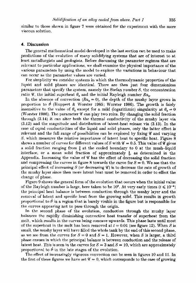
In the absence of convection (Ra, = 0 ) , the depth of the mushy layer grows in proportion to ti (Huppert & Worster 1985; Worster 1986). The growth is fairly insensitive to the value of 8, except for a mild (logarithmic) singularity a t 6, = 0 (Worster 1986). The parameter U can play two roles. By changing the solid fraction through (3.14) it can alter both the thermal conductivity of the mushy layer via (3.12) and the magnitude and distribution of latent-heat release via (3.13). In the case of equal conductivities of the liquid and solid phases, only the latter effect is relevant and the full range of possibilities can be explored by fixing V and varying S , which measures the relative importance of latent heat to specific heat. Figure 8 shows a number of curves for different values of S with % = 0.5. This value of W gives a solid fraction ranging from $ at the cooled boundary to 0 at the mush-liquid interface, or a mean solid fraction of approximately $, as determined in the Appendix. Increasing the value of U has the effect of decreasing the solid fraction and compressing the curves in figure 8 towards the curve for S = 0. We see that the principal effect of increasing S (or decreasing U ) is to decrease the rate of growth of the mushy layer since then more latent heat must be removed in order to effect the change of phase.

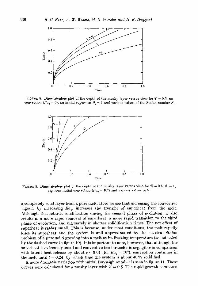
Figure 9 shows the general form of the evolution that occurs when the initial value of the Rayleigh number is large, here taken to be lo0. At very early times ( t < the principal heat balance is between conduction through the mushy layer and the removal of latent and specific heat from the growing solid. This results in growth proportional to I$ in a region that is barely visible in the figure but is responsible for the curves appearing not to pass through the origin.

In the second phase of the evolution, conduction through the mushy layer balances the rapidly diminishing convective heat transfer of superheat from the melt, which results in the curves being concave upwards. This phase lasts until most of the superheat in the melt has been removed a t t = 0.01 (see figure 12). When S is small, the mushy layer will have filled the whole tank by the end of this second phase, as we see from the curves for S = 0 and S = 1. However, when S is larger, a third phase ensues in which the principal balance is between conduction and the release of latent heat. This is seen in the curves for S = 3 and S = 10, which are approximately proportional to ti in the late stages of the evolution.

The effect of increasingly vigorous convection can be seen in figures 10 and 11. In the first of these figures we have set %? = 0, which corresponds to the case of growing

336 R. C. Kerr, A . W. Woods, M . G . Worster and H . E. Huppert

0.8 -

-

-

I I I I

0 0.2 0.4 0.6 0.8 1 .O Time

FIQURE 8. Dimensionless plot of the depth of the mushy layer versus time for W = 0.5, no convection (Ra, = 0 ) , an initial superheat 0, = 1 and various values of the Stefan number S.

1.0 I I 1 I I I 1 .o I 1 I I

n

I I 0 0.2 0.4 0.6 0.8 I .o 0 0.2 0.4 0.6 0.8 I .o

Time

FIQURE 9. Dimensionless plot of the depth of the mushy layer versus time for W = 0.5, 8, = I , vigorous initial convection (Ra, = 10') and various values of 8.

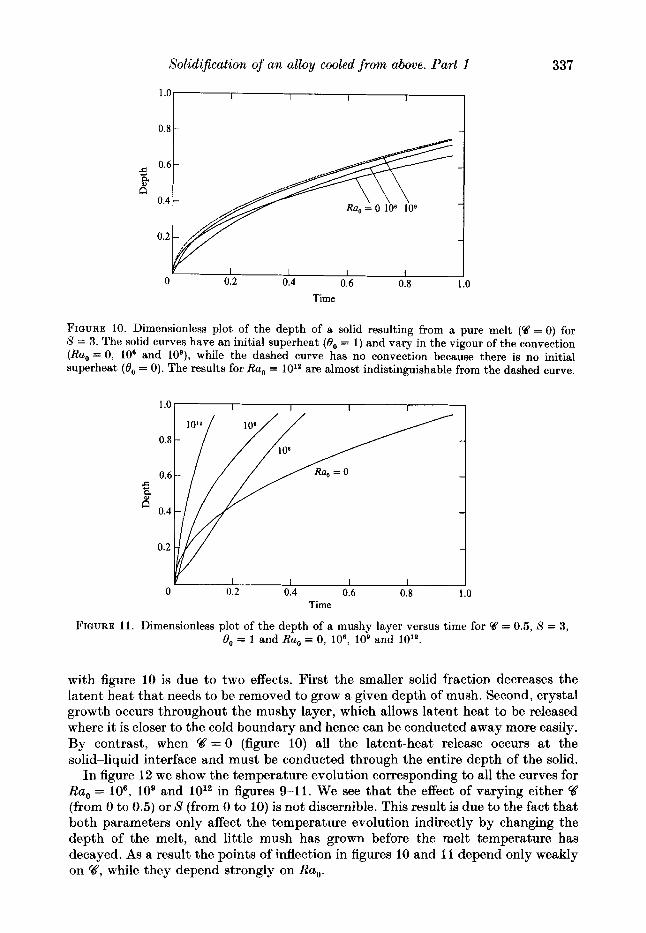
a completely solid layer from a pure melt. Here we see that increasing the convective vigour, by increasing Ra,, increases the transfer of superheat from the melt. Although this retards solidification during the second phase of evolution, it also results in a more rapid removal of superheat, a more rapid transition to the third phase of evolution, and ultimately in shorter solidification times. The net effect of superheat is rather small. This is because, under most conditions, the melt rapidly loses its superheat and the system is well approximated by the classical Stefan problem of a pure solid growing into a melt a t its freezing temperature (as indicated by the dashed curve in figure 10). It is important to note, however, that although the superheat is extremely small and convective heat transfer is negligible in comparison with latent-heat release by about & = 0.01 (for Ra, = lo@), convection continues in the melt until t = 0.24, by which time the system is about 40% solidified.

A more dramatic variation with initial Rayleigh number is seen in figure 11. These curves were calculated for a mushy layer with %? = 0.5. The rapid growth compared

Solidification of an alloy cooled from above. Part 1

0.8 l ’ O 1

337

Time

FIGURE 10. Dimensionless plot of the depth of a solid resulting from a pure melt (U = 0) for S = 3. The solid curves have an initial superheat (0, = 1) and vary in the vigour of the convection (Ra, = 0, 10‘ and lo’), while the dashed curve has no convection because there is no initial superheat (0, = 0). The results for Ra, = 10l2 are almost indistinguishable from the dashed curve.

Time

FIGURE 11. Dimensionless plot of the depth of a mushy layer versus time for W = 0.5, S = 3, 0, = 1 and Ru, = 0, lo6, loB and 10l2.

with figure 10 is due to two effects. First the smaller solid fraction decreases the latent heat that needs to be removed to grow a given depth of mush. Second, crystal growth occurs throughout the mushy layer, which allows latent heat to be released where it is closer to the cold boundary and hence can be conducted away more easily. By contrast, when V = O (figure 10) all the latent-heat release occurs a t the solid-liquid interface and must be conducted through the entire depth of the solid.

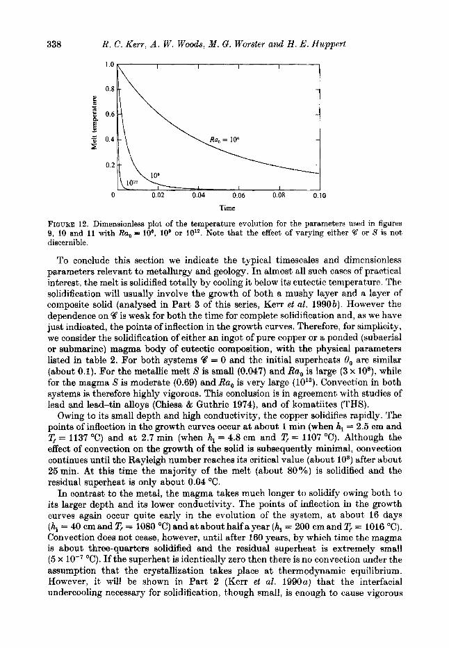
In figure 12 we show the temperature evolution corresponding to all the curves for Ra, = lo6, lo9 and 10l2 in figures 9-11. We see that the effect of varying either V (from 0 to 0.5) or X (from 0 to 10) is not discernible. This result is due to the fact that both parameters only affect the temperature evolution indirectly by changing the depth of the melt, and little mush has grown before the melt temperature has decayed. As a result the points of inflection in figures 10 and 11 depend only weakly on V, while they depend strongly on Ra,.

338 R. C . Kerr, A . W. Woods, M . G . Worster and H . E. Huppert

I L 1

0 0.02 0.04 0.06 0.08 0.10

Time

FIGURE 12. Dimensionless plot of the temperature evolution for the parameters used in figures 9, 10 and 11 with Ra, = lod, lo8 or 10". Note that the effect of varying either V or S is not discernible.

To conclude this section we indicate the typical timescales and dimensionless parameters relevant to metallurgy and geology. In almost all such cases of practical interest, the melt is solidified totally by cooling it below its eutectic temperature. The solidification will usually involve the growth of both a mushy layer and a layer of composite solid (analysed in Part 3 of this series, Kerr et al. 1990b). However the dependence on W is weak for both the time for complete solidification and, as we have just indicated, the points of inflection in the growth curves. Therefore, for simplicity, we consider the solidification of either an ingot of pure copper or a ponded (subaerial or submarine) magma body of eutectic composition, with the physical parameters listed in table 2. For both systems W = 0 and the initial superheats 0, are similar (about 0.1). For the metallic melt 8 is small (0.047) and Ra, is large (3 x lo8), while for the magma S is moderate (0.69) and Ra, is very large (l0ls). Convection in both systems is therefore highly vigorous. This conclusion is in agreement with studies of lead and lead-tin alloys (Chiesa & Guthrie 1974), and of komatiites (THS).

Owing to its small depth and high conductivity, the copper solidifies rapidly. The points of inflection in the growth curves occur at about 1 min (when hi = 2.5 cm and

= 1137 "C) and at 2.7 min (when hi = 4.8 cm and T, = 1107 "C). Although the effect of convection on the growth of the solid is subsequently minimal, convection continues until the Rayleigh number reaches its critical value (about lo3) after about 25 min. At this time the majority of the melt (about 80%) is solidified and the residual superheat is only about 0.04 "C.

In contrast to the metal, the magma takes much longer to solidify owing both to its larger depth and its lower conductivity. The points of inflection in the growth curves again occur quite early in the evolution of the system, at about 16 days (hi = 40 cm and T( = 1080 "C) and at about half a year (hi = 200 cm and T / = 1016 "C). Convection does not cease, however, until after 160 years, by which time the magma is about three-quarters solidified and the residual superheat is extremely small (5 x lo-' "C). If the superheat is identically zero then there is no convection under the assumption that the crystallization takes place a t thermodynamic equilibrium. However, it will be shown in Part 2 (Kerr et al. 1 9 9 0 ~ ) that the interfacial undercooling necessary for solidification, though small, is enough to cause vigorous

Solidi$cation of an alloy cooled from above. Part I 339

Units

O C

"C "C ern J OC-'

J ~ m - ~ O C - l

W cm-' O C - l

W cm-' "C-l J ~ m - ~ om2 s-l "C-1 -

Metal

1185 1085 0 30 29 30 2.44 1.66 1700 0.004

0.056 2 x 10-4

Magma

1100 1000 0

2.0 2.0 0.01 0.01 1350 100

0.056

104

5 x 10-5

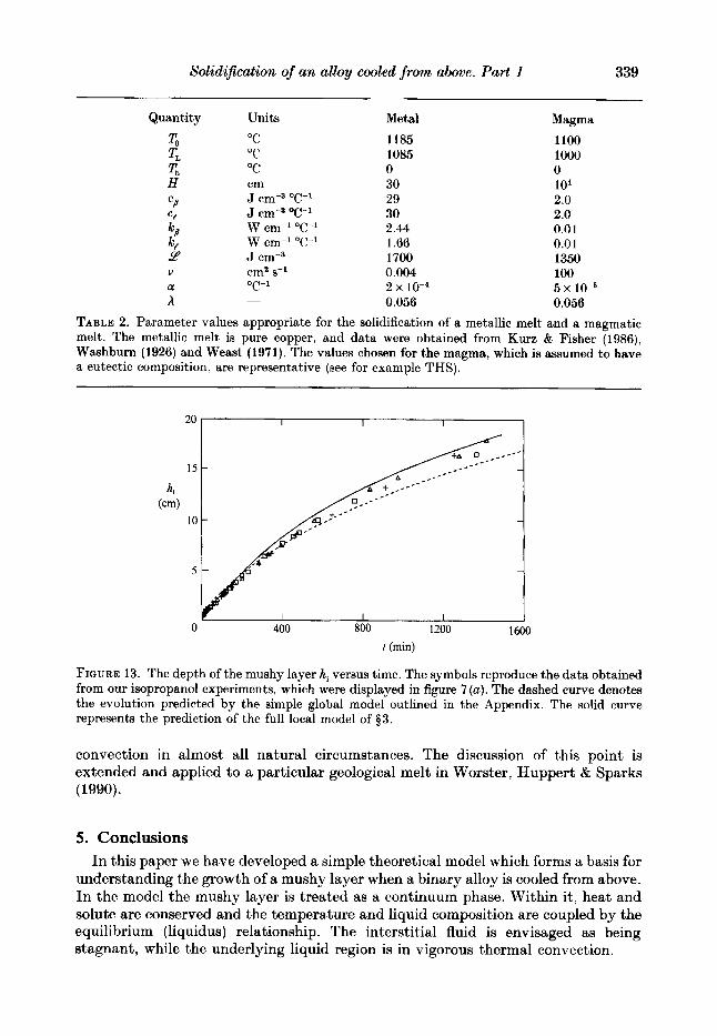
TABLE 2. Parameter values appropriate for the solidification of a metallic melt and a magmatic melt. The metallic melt is pure copper, and data were obtained from Kurz & Fisher (1986), Washburn (1926) and Weast (1971). The values chosen for the magma, which is assumed to have a eutectic composition, are representative (see for example THS).

I I I I

t (min)

FIGURE 13. The depth of the mushy layer hi versus time. The symbols reproduce the data obtained from our isopropanol experiments, which were displayed in figure 7 (a). The dashed curve denotes the evolution predicted by the simple global model outlined in the Appendix. The solid curve represents the prediction of the full local model of $3.

convection in almost all natural circumstances. The discussion of this point is extended and applied to a particular geological melt in Worster, Huppert & Sparks (1990).

5. Conclusions In this paper we have developed a simple theoretical model which forms a basis for

understanding the growth ofa mushy layer when a binary alloy is cooled from above. In the model the mushy layer is treated as a continuum phase. Within it, heat and solute are conserved and the temperature and liquid composition are coupled by the equilibrium (liquidus) relationship. The interstitial fluid is envisaged as being stagnant, while the underlying liquid region is in vigorous thermal convection.

340 R. C. Kerr, A . W . Woods, M . G . Worster and H . E . Huppert

To test the model we performed a number of experiments with a particular solution of water and isopropanol, which offered few complications and for which reliablc thermodynamic data were available. Both the thickness of the growing mushy layer and the temperature of the underlying convecting solution were measured, and their evolution was found to be well fitted by the predictions of our theoretical model. This result suggests that the model incorporates correctly the three governing thermodynamic processes : the extraction of heat from the system through the mushy layer by thermal conduction; the internal growth of the mushy layer with the consequent release of latent heat; and the heat extracted at the interface from the underlying melt. I n the Appendix we show how the same fundamental thermodynamic processes can be approximated, using integral constraints derived from the basic model, to achieve results that may well be adequate for many practical applications.

Despite the close agreement between theory and experiment, it is clear from figure 7 ( b ) that the model systematically overestimates the temperature of the melt. Although the discrepancy is small, it is particularly significant that in the experiments the melt became supersaturated, a possibility not allowed for in the theory. The disequilibrium of the melt can, in other systems, cause different phenomenona to occur. In Part 2 of this series of papers (Kerr et al. 1990a), we shall extend our model to account for disequilibrium effects in the melt and explore the consequences for the solidifying system.

We wish to thank Mark Hallworth for his technical assistance with the laboratory experiments. A. B. Crowley, J. Dantzig, A. Hoadley, D. T. J. Hurle, C. Jaupart and J. S. Turner provided valuable comments and reviews. We gratefully acknowledge research fellowships from the following Cambridge Colleges : Churchill (R. C. K.), Trinity (M.G.W.) and St John’s (A.W.W.), and financial support from the BP Venture Research Fund (H.E. H.). A. W. W. is also grateful for support as a Green Scholar a t IGPP, Scripps Institution of Oceanography during the final stages of the research.

Appendix In this Appendix, we examine the procedure of simplifying the model of the mushy

layer so that it relies only on global conservation of heat and solute. This approach was employed by Huppert & Worster (1985) to develop a model which predicted accurately the rate of growth of ice when aqueous solutions of various salts were cooled from below, The primary advantage of this approach is that it avoids the necessity of solving the partial differential equation for heat conduction in the mushy layer. The resulting equations are therefore much easier to compute.

The method adopts a simple trial function for the solid fraction within the mushy layer. Here, as in Huppert & Worster (1985), we choose

$ = constant (0 < x d hi). (A 1)

We estimate the conductive heat flux through the mushy layer by assuming a linear temperature profile, which is consistent with (A 1) in the limit of large Stefan number. An equation expressing the global conservation of solute is obtained from

Solidi$cation of an alloy cooled from above. Part 1 341

(3.4) by integrating it with respect to time and then with respect to height across the whole depth of the domain. This yields the dimensionless constraint

( l -$ ) - edz+$% = 0. hi l . r

With the approximate function 8 = (z/hi) - 1, this yields

1 $ = $ =- - 2%+1'

A set of ordinary differential equations describing the system is then given by (3.20) coupled with

which is the equivalent of (3.19). The differential equations were solved using a fourth-order, Runge-Kutta method

starting from asymptotic expansions of the solutions. The results for the depth of the mushy layer hi are shown in figure 13 where they are compared to both the data obtained from our experiments with isopropanol and with the results of the detailed model of Q 3. The evolution of the temperature of the liquid region el, as predicted by the simple model of this Appendix, is indistinguishable from that shown in figure 7 (a). The agreement shown in figure 13 illustrates how the use of integral constraints applied to trial functions can give good approximate results for some of the gross features of the evolution of the system.

When using the global model it is important to understand the nature of the approximations that have been made. For example, the adoption of a linear temperature profile assumes that the timescale for cooling by conduction H 2 / ~ is small in comparison either with the timescale for removal of latent heat by conduction Sfla/, or with the timescale for cooling by convection R a - i H 2 / ~ . This is an excellent approximation at moderate or large Stefan numbers. It is clearly inappropriate, howe$er, if both the Stefan number is small, so that the release of latent heat is negligible, and the Rayleigh number is simultaneously large, resulting in the rapid loss of superheat.

The assumption of a constant solid fraction implies that the latent heat is all released a t the mush-liquid interface. This is exact for +? = 0, corresponding to a solid fraction of unity, but is increasingly inaccurate as %9 increases and the solid fraction 4, decreases. In reality, the release of latent heat is distributed throughout the mushy layer, nearer to the cooled boundary through which it must ultimately be conducted. This particular approximation therefore underestimates the rate of growth. A second effect of the assumption of a constant solid fraction is that it leads to an overestimate of the effective conductivity of the mushy layer whenever the conductivities of the solid and liquid phases are unequal. These two effects of the same assumption can therefore partly counteract each other.

The result of all these approximations is that the global model has given us predictions for the growth of mushy layers from aqueous solutions that have been accurate to within about 10 YO.

R . G . Kerr, A . W. Woods, M . G. Worster and H . E . Huppert

R E F E R E N C E S

ABEGG, R. 1894 Studien iiber Gefrierpunkte Konzentrierter Losungen. 2. Phys. Chem. 15,

ARIES, W. F. 1977 Numerical Methods for Pa,rtial Diferential Equations (2nd edn.). Academic. CHEN, C. F. & TURNER, J. S. 1980 Crystallization in a double-diffusive system. J . Geophys. Res.

CHIESA, F. M. & GUTHRIE, R. I. 1,. 1974 Eatural convective heat transfer rates during the solidification and melting of metals and alloy systems. Tram. ASME J . Heat Transfer 96,

DENTON, R. A. & WOOD, I. R. 1979 Turbulent convection between two horizontal plates. Intl J .

FLEMINGS, M. C . 1974 RolidiJication Processing. McGraw-Hill. HUPPERT, H. E. & WORSTER, M. G. 1985 Dynamic solidification of a binary melt,. Nature 314,

KAYE, G. W.C. & LABY, T. H. 1973 Tables of Physical and Chemical Constants and some Mathematical Functions. Longman.

KERR, R. C., WOODS, A. W., WORSTER, M. G. & HUPPERT, H. E. 1989 Disequilibrium and macrosegregation during the solidification of a binary melt. Nature 340, 357-362.

KERR, R. C., WOODS, A. W., WORSTER, M. G. & HUPPERT, H. E. 1990a Solidification of an alloy cooled from above. Part 2. X6n-equilibrium interfacial kinetics. J . Fluid Mech. 217, 331-348.

KERR, R. C., WOODS, A. W., WORSTER, M. G. & HUPPERT, H. E. 1990b Solidification of an alloy cooled from above. Part 3. Compositional stratification within the solid. J . Fluid Mech. 218, (in press).

KURZ, W. & FISHER, D. J. 1986 Fundamentals of #olidi$cation. Trans. Tech. Publications. TURNER, J . S. 1979 Buoyancy Effects in Fluids. Cambridge University Press. TURNER, J. S., HUPPERT, H. E. & SPARKS, R. S. J. 1986 Komatiites 11: Experimental and

theoretical investigations of' post-emplacement cooling and crystallization. J . Petrol. 27, 397437 (referred to herein as THS).

VARGAFTIK, N. 13. 1975 Tables on the Thermodynamic Properties of Liquids and Gases. John Wiley BE Sons.

WASHBURN, E. W. (ED.) 1926 International Critical Tables of Numerical data: I'hysics, Chemistry and Technology. National Academic Press.

WEAST, R. C. (ED.) 1971 CRC Handbook of Chemistry and Physics. The Chemical Rubber Co. WORSTER, M. G . 1986 Solidification of an alloy from a cooled boundary. J . Fluid Mech. 167,

WORSTER, M. G., HUPPERT, H. E. & SPARKS, R. S. J. 1990 Convection and crystallization in

209-261.

85, 2573-2593.

377-384.

Heat Mass Transfer 22, 1339-1346.

703-707.

481-501.

magma cooled from above. Earth Planet. Sci. Lett. (sub judice).