Solidification kinetics in undercooled pure iron and iron-boron … · 2016-07-04 ·...
120
SOLIDIFICATION KINETICS IN UNDERCOOLED PURE IRON AND IRON-BORON ALLOYS UNDER DIFFERENT FLUID FLOW CONDITIONS DISSERTATION zur Erlangung des Grades eines Doktors der Naturwissenschaften in der Fakultät für Physik und Astronomie der Ruhr-Universität Bochum von Christian Karrasch aus Bonn Bochum 2016
Transcript of Solidification kinetics in undercooled pure iron and iron-boron … · 2016-07-04 ·...

SOLIDIFICATION KINETICS IN UNDERCOOLED
PURE IRON AND IRON-BORON ALLOYS
UNDER DIFFERENT FLUID FLOW
CONDITIONS
DISSERTATION
zur
Erlangung des Grades
eines Doktors der Naturwissenschaften
in der Fakultät für Physik und Astronomie
der Ruhr-Universität Bochum
von
Christian Karrasch
aus
Bonn
Bochum 2016

1. Gutachter: Prof. Dr. Dieter M. Herlach
2. Gutachter: Prof. Dr. Kurt Westerholt
Datum der Disputation: 28. Januar 2016

TO KAROLINA AND MY FAMILY


We are at the very beginning of time for human race.
It is not unreasonable that we grapple with problems.
But there are tens of thousands of years in the future.
Our responsibility is to do what we can, learn what we can,
Improve the solutions, and pass them on.
RICHARD P. FEYNMAN (1918-1988)
CONTENTS
INTRODUCTION .................................................................................................................................................................. 1
1 THEORETICAL BACKGROUND: SOLIDIFICATION IN UNDERCOOLED LIQUIDS ............................ 5
1.1 Thermodynamics: Undercooling and Driving Force for Solidification ..................................... 6
1.2 Thermodynamics of Binary Systems ...................................................................................................... 7
1.3 Nucleation Theory .......................................................................................................................................... 8
1.3.1 Homogeneous Nucleation .................................................................................................................. 8
1.3.2 Heterogeneous Nucleation ............................................................................................................. 13
1.3.3 Nucleation in Alloys .......................................................................................................................... 14
1.4 Solid-Liquid Interface ................................................................................................................................ 15
1.5 Local Equilibrium to Non-Equilibrium Solidification ................................................................... 18
1.5.1 GIBBS-THOMSON Effect and the Morphology of the Solid-Liquid Interface .................. 18
1.5.2 Attachment Kinetics at the Solid-Liquid Interface ............................................................... 20
1.5.3 Solute Trapping ................................................................................................................................... 22
2 DENDRITIC GROWTH MODEL ......................................................................................................................... 25
2.1 Sharp Interface Model for Dendritic Solidification ........................................................................ 26
2.2 Influence of Convection on Dendrite Growth .................................................................................. 32
3 EUTECTIC GROWTH MODEL ............................................................................................................................ 35
3.1 Current Model for Concentrated Alloys with Non-Linear Phase Diagram (NLPD) .......... 37
3.2 Model of Li and Zhou (LZ) for Dilute Alloys with Linear Phase-Diagram (LPD) ............... 40
3.3 Kinetic Liquidus Slopes for Large Undercoolings .......................................................................... 41
4 EXPERIMENTAL METHODS .............................................................................................................................. 45
4.1 Electromagnetic Levitation (1g-EML) ................................................................................................. 45
4.2 Electromagnetic Levitation under Reduced Gravity (µg-EML) ................................................ 48
4.3 Melt-Fluxing in a Static Magnetic Field (MF) ................................................................................... 51
4.4 Infrared Camera (IRC) versus High-Speed Camera (HSC) .......................................................... 53
4.5 Microstructure Analysis ............................................................................................................................ 55

5 SAMPLE SYSTEM: IRON-BORON ..................................................................................................................... 57
5.1 Phase Diagram, Material Parameter, and Crystallographic Structure ................................... 57
5.2 Sample Material and Preparation for Experiments and Microstructure Analysis............ 59
6 EXPERIMENTAL RESULTS AND DISCUSSION ........................................................................................... 61
6.1 Growth Morphology and Microstructure........................................................................................... 61
6.2 Bent Dendrite Growth ................................................................................................................................ 65
6.2.1 Bent growing dendrites under reduced gravity conditions ............................................. 65
6.2.2 Microstructure of bent dendrites ................................................................................................ 66
6.2.3 Discussion ............................................................................................................................................. 66
6.2.4 Conclusion ............................................................................................................................................. 68
6.3 Dendrite Growth Velocity 𝑽 versus Undercooling ∆𝑻 .................................................................. 69
6.3.1 Pure Fe .................................................................................................................................................... 70
6.3.2 Fe-1 at.% B ............................................................................................................................................ 76
6.3.3 Fe-5 at.% B ............................................................................................................................................ 83
6.3.4 Fe-10 at.% B ......................................................................................................................................... 86
6.4 Eutectic composition Fe-17 at.% B ....................................................................................................... 89
6.4.1 Eutectic Dendrite Growth Velocities 𝒗(∆𝑻) ............................................................................ 89
6.4.2 Microstructure Analysis of Fe-17 at.% B .................................................................................. 96
SUMMARY .......................................................................................................................................................................... 97
A APPENDIX .............................................................................................................................................................. 101
A.1 Video Analysis of Dendrite Growth Velocity ................................................................................. 101
BIBLIOGRAPHY ............................................................................................................................................................. 103
Publication List ............................................................................................................................................................. 112
Curriculum Vitae .......................................................................................................................................................... 114
Acknowledgments ....................................................................................................................................................... 113

1 INTRODUCTION
INTRODUCTION
Our daily life is surrounded by materials which were formed during phase transformation, such
as ice, steel constructions of buildings, and even crack resistant display-glass of smartphones.
Since the Bronze Age (4000 BC – 1200 BC) followed by the Iron Age (1200 BC – 500 BC) the use
of solidification techniques, alloying and casting play a key role in human history. For example
the legendary Damascus steel swords are known for their sharpness and strength. This material
culture of mankind is culminated in our today’s high technology society. However, not before the
first half of the 20th century scientists tried to develop a physical understanding how the
material properties were related to the conditions of solidification.
In the case of metals the major growth mode is dendritic solidification (tree-like). “Worldwide, as
many as 10 billion metallic dendrites are produced in industry every second” [1]. In other
words, to understand and to control dendritic solidification processes is of great economic
interest. Particularly the initial process conditions determine the evolution of the microstructure
and therefore influence the final product of solidification. The main challenge is to design
materials directly from the melt with specific material properties without expensive post-
processing. Therefore it is essential to have a fundamental physical understanding of the
complex mechanism of dendritic solidification which is mainly governed by the heat and mass
transport at the moving solid-liquid interface. Even though dendrite growth is an experimentally
and theoretically well investigated process, there are still many open questions in this field of
solidification science [2].
Since ISAAC NEWTON (1643-1727) studied snowflakes under a microscope the process how
dendritic structures form out of chaos is not fully understood. In particular, side branches of
dendrites have a self-similar pattern and fractal geometry. NEWTON investigated ice crystals and
their identification which were formed in clouds under various environmental conditions. In
order to understand the laws of nature he supposed an underlying surface order to explain this
manifold phenomenon. In general, the mechanism of dendritic growth is driven by temperature
and or concentration gradients at the solid-liquid interface. Initially solid fluctuations into the
liquid at the growth front of a crystal are able to grow faster as other parts. Those tips dash
forward becoming a dendritic stem which can build further side branches leading to a network
structure with residual liquid in between. In detail, dendrite growth is a complex process dealing
with many aspects as follows:
Diffusion of heat and mass
Solubility of the chemical components in the solid
Atomic attachment kinetics at the interface between liquid and solid
2 INTRODUCTION
Shape, curvature and stability of the interface
Surface energy of the interface and its anisotropy
Concentration and thermal convection.
In order to understand dendritic solidification kinetics in more detail it is important to measure
key factors as for instance the growth velocity 𝑉 over a wide range of magnitude and therefore
verify dendrite growth models. Non-equilibrium rapid solidification offers this possibility. In
1724 GABRIEL FAHRENHEIT discovered an effect called undercooling ∆𝑇. He observed water
droplets which stayed liquid below their freezing temperature of 0 °C. In a clean environment a
high purity material remains liquid in a metastable undercooled state unless hundreds of atoms
cluster statistically together and form a stable nucleus which starts to grow. Statistical
nucleation theory tells you which phase nucleates with a certain possibility. Thermodynamics
defines the equilibrium state of coexisting liquid and solid phase whereas growth theory
describes the kinetics of growth. The opportunity of undercooling offers to study dendritic
solidification far from thermal equilibrium over a wide range of undercooling. The dependence
of 𝑉(∆𝑇) varies for metals from 𝑐𝑚/𝑠 up to several 𝑚/𝑠 depending on the undercooling from
50 𝐾 to above 300 𝐾 prior to equilibrium solidification.
Rapid solidification in undercooled melts can be investigated by containerless experimental
methods where heterogeneous nucleation on container walls is completely avoided which
otherwise limits the undercoolability of a melt. For instance electromagnetic levitation (EML)
technique [3] is applied to undercool droplets of metallic melt accessible for in-situ diagnostics
of the solidification process. During the transformation of the undercooled liquid phase into the
solid phase latent heat is released leading to a visible contrast between liquid and solid which is
recordable by a high-speed video camera. In the past infrared cameras were to slow for
observing crystal growth in metals. Recent developments make fast infrared cameras available.
As feasibility study within this thesis an infrared camera is used to evaluate it as a powerful tool
for new findings. This is especially interesting for low melting materials at small undercooling
with weak contrast in visible light.
Understanding industrial multicomponent alloys is a very complex issue. To study dendritic
growth and investigate effects of solidification, a binary system like Fe-B is used as a model
system. Moreover the knowledge of the solidification behaviour and thermodynamic properties
of Fe-B is of interest in several fields of material engineering. For example, Fe-B is a subsystem of
the Nd-Fe-B alloys with superior magnetic properties. Also the high modulus TiB2-reinforced
steel composite is based on the Fe-B-Ti ternary alloy. Furthermore B is used for hardenability of
steels and even to form amorphous alloys. In this thesis the growth kinetics of pure Fe and Fe-B
alloys are investigated by measuring the growth velocity 𝑉 as a function of undercooling ∆𝑇. In
3 INTRODUCTION
general, dendritic solidification in undercooled melts is mainly governed by nucleation and
crystal growth. Namely the interfacial energy, the interfacial mobility and the crystal anisotropy
are key factors for dendrite growth kinetics and dendritic morphology which will be
investigated in the present work by measuring and modelling 𝑉(∆𝑇). The anisotropic nature of
the interfacial free energy and atomic attachment kinetics lead to a preferred growth direction
of the dendritic crystal. In the case of a cubic crystal structure like Fe the ⟨100⟩ −direction is
typical [4]. The knowledge of the growth morphology is crucial to analyse EML dendrite growth
videos where only the intersection of the solidification front with the spherical sample surface is
visible. In detail, the pattern visible on the surface is the intersection of a growing octahedron of
which the center is placed on the sample surface [5]. The vertices correspond to the primary
dendrite tips and the edges correspond to the secondary side branches.
Pure Fe melts crystallize primarily in body-centered cubic phase. The Fe-B system is an
incongruent melting metal-metalloid alloy at low B concentrations. Starting with pure Fe
manifold phenomena can be studied by stepwise adding B. In general, B is poorly soluble in Fe
[6] and has a low equilibrium partition coefficient 𝑘𝐸 ≪ 1. During solidification the different
solubility of solvent in liquid and solid phase leads to a pile up of B concentration and a
concentration gradient in front of the moving interface. Due to the low solubility of B in Fe the
dendrite growth velocity is limited by the diffusion of B in liquid Fe. At low undercoolings this
effect dominates, and slows down dendrite growth velocity leading to a Fe-B solid solution. For
larger undercoolings at low B concentration (such as Fe-1 at.% B) an effect called solute trapping
is expected. At a certain undercooling the rapid propagation of the solid-liquid interface leads to
entrapment of solute beyond its chemical equilibrium solubility. B is incorporated above its
solubility limit in Fe leading to a supersaturated solid solition. This non-equilibrium
phenomenon (solute trapping) can be explained and treated by the sharp interface model taking
into account a velocity dependent partition coefficient 𝑘(𝑉).
At higher B concentrations the growth velocity is expected to slow further down. Additionally
the primary crystallization mode changes from body-centered cubic (bcc) to face-centered cubic
(fcc) structure (Fe-5 and 10 at.% B). In this case a phase competition in nucleation and growth
takes place between bcc and fcc structure. Measurements of dendrite growth velocity as a
function of undercooling may help to give a phase discrimination.
By further increasing the B concentration (Fe-17 at.% B) the single phase dendritic mode
changes to the multiphase eutectic growth mode in which two different crystallographic phases
are formed simultaneously during solidification. The eutectic composition Fe-17 at.% B is a
metallic glass former which gives rise to investigations of glass formation. Even nucleation and
crystallization may be suppressed by applying sufficiently high external cooling rates. However

4 INTRODUCTION
the glass transition temperature 𝑇𝑔 of Fe-17 at.% B is about 800 𝐾 [7] and cannot be reached by
the experimental methods applied within this thesis. Amorphous Fe-17 at.% B may be prepared
at much higher cooling rates (~106 𝐾 𝑠−1).
Melt convection is an important aspect which affects dendritic growth at high fluid flow
velocities. In earth laboratory, high electromagnetic fields are necessary in a terrestrial 1g-EML
to lift the sample against gravity. Therefore electromagnetic stirring induces fluid flow which
affects the heat and mass transport at the solid-liquid interface during solidification. This
influence of forced convection changes dendritic growth morphology and growth velocity,
especially if the fluid flow velocity is in the same order of magnitude or larger than the
solidification velocity itself. The present research shows unexpected bent dendrite growth under
different fluid flow conditions which was accepted for publication [8]. This phenomenon has
been observed in-situ for the first time in solidifying metals during levitation. Bent dendrite
growth appears at low undercooling for all investigated dendritic growing alloys (Fe-1, 5, and 10
at.% B). In the present work the influence of convection on growth velocity and morphology is
investigated by applying different experimental fluid flow conditions:
1g-EML (0.3 𝑚/𝑠 ) [9]
µg-EML (0.05 𝑚/𝑠) [9] under reduced gravity during parabolic flight
Melt-fluxing experiments in a static magnetic field (0 − 6 𝑇).

5 THEORETICAL BACKGROUND: SOLIDIFICATION IN UNDERCOOLED LIQUIDS
God created the solids,
The Devil their surfaces.
WOLFGANG PAULI (1900-1958)
1 THEORETICAL BACKGROUND: SOLIDIFICATION IN UNDERCOOLED LIQUIDS
In this chapter the thermodynamic background is described in order to understand non-
equilibrium rapid solidification processes. Together with chapter 2 dendritic growth and chapter
3 eutectic growth it builds the fundament to interpret the experimental results. For further and
more detailed explanations the author refers to i.e. the book SOLIDIFICATION by J. A. DANTZIG
and M. RAPPAZ [10] or METASTABLE SOLIDS FROM UNDERCOOLED MELTS by D.M. HERLACH, P.
GALENKO and D. HOLLAND-MORITZ [11].
Thermodynamics characterizes the equilibrium state of liquid and solid phase. However a system
in thermodynamic equilibrium would not change in a macroscopic view. There has to be a
deviation from equilibrium, otherwise solid and liquid will coexist at the melting temperature
with no moving of the phase boundary. For instance, lowering the temperature of the system
results in an expansion of the stable phase (solid) at the expense of the unstable phase (liquid).
In other words, the crystal grows into the melt. In this case the liquid at the interface is
undercooled. Rapid Solidification from a deeply undercooled liquid state is a non-equilibrium
process which is governed by nucleation and crystal growth. In order to initiate solidification a
nucleus of critical size has to be formed in the undercoolded melt. Nucleation theory predicts
which crystallographic phase is selected and defines the probability of atoms which statistically
cluster together to form a nucleus. After a nucleus of critical size is formed it becomes stable by
further growth which is described by crystal growth theory. Subsequently, the solid state
expands by crystal growth that is either dendritic or eutectic. The driving force for solidification
is the GIBBS free energy which will be defined in this chapter. In general, with increasing
undercooling the driving force for solidification increases which leads to a faster growth of the
solid phase.
6 THEORETICAL BACKGROUND: SOLIDIFICATION IN UNDERCOOLED LIQUIDS
1.1 Thermodynamics: Undercooling and Driving Force for Solidification
The equilibrium state of a thermodynamic system can be described by the thermodynamic
potential. In case of choosing temperature 𝑇, pressure 𝑝, and particle number N, as
thermodynamic variables the GIBBS free energy 𝐺(𝑝, 𝑇, 𝑁) is the thermodynamic potential. It
describes the changes of the system is the GIBBS free energy 𝐺(𝑝, 𝑇, 𝑁). The GIBBS free energy 𝐺
is defined by:
𝐺(𝑝, 𝑇, 𝑁) = 𝑈(𝑆, 𝑉, 𝑁) + 𝑝 ∙ 𝑉⏟ 𝐻(𝑆,𝑁,𝑝)
− 𝑇 ∙ 𝑆(𝑈, 𝑉, 𝑁) = 𝐻 − 𝑇 ∙ 𝑆,
where 𝑈 is the internal energy of the system, 𝑉 the volume, 𝑆 the entropy, and 𝐻 the enthalpy.
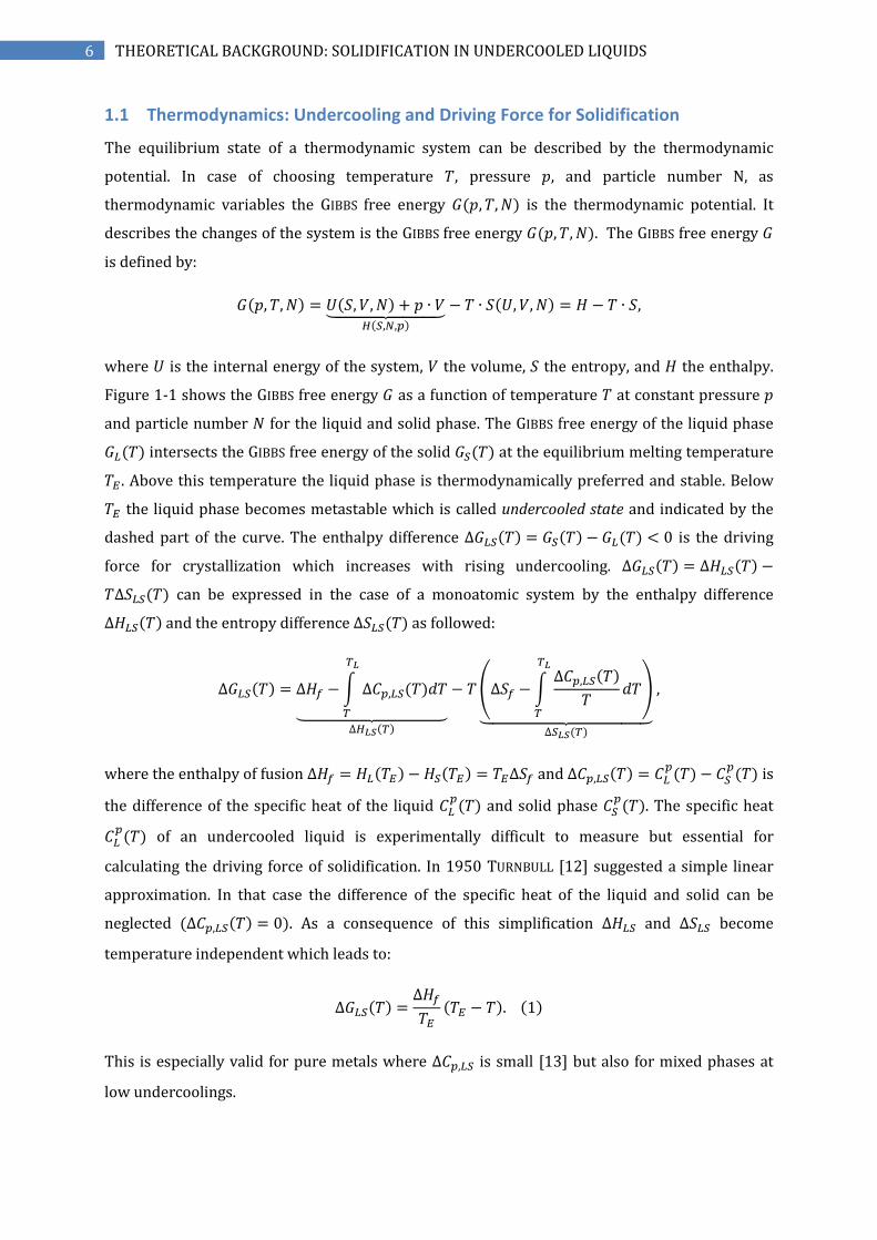
Figure 1-1 shows the GIBBS free energy 𝐺 as a function of temperature 𝑇 at constant pressure 𝑝
and particle number 𝑁 for the liquid and solid phase. The GIBBS free energy of the liquid phase
𝐺𝐿(𝑇) intersects the GIBBS free energy of the solid 𝐺𝑆(𝑇) at the equilibrium melting temperature
𝑇𝐸 . Above this temperature the liquid phase is thermodynamically preferred and stable. Below
𝑇𝐸 the liquid phase becomes metastable which is called undercooled state and indicated by the
dashed part of the curve. The enthalpy difference ∆𝐺𝐿𝑆(𝑇) = 𝐺𝑆(𝑇) − 𝐺𝐿(𝑇) < 0 is the driving
force for crystallization which increases with rising undercooling. ∆𝐺𝐿𝑆(𝑇) = ∆𝐻𝐿𝑆(𝑇) −
𝑇∆𝑆𝐿𝑆(𝑇) can be expressed in the case of a monoatomic system by the enthalpy difference
∆𝐻𝐿𝑆(𝑇) and the entropy difference ∆𝑆𝐿𝑆(𝑇) as followed:
∆𝐺𝐿𝑆(𝑇) = ∆𝐻𝑓 −∫ ∆𝐶𝑝,𝐿𝑆(𝑇)𝑑𝑇
𝑇𝐿
𝑇⏟ ∆𝐻𝐿𝑆(𝑇)
− 𝑇(∆𝑆𝑓 −∫∆𝐶𝑝,𝐿𝑆(𝑇)
𝑇𝑑𝑇
𝑇𝐿
𝑇
)
⏟ ∆𝑆𝐿𝑆(𝑇)
,
where the enthalpy of fusion ∆𝐻𝑓 = 𝐻𝐿(𝑇𝐸) − 𝐻𝑆(𝑇𝐸) = 𝑇𝐸∆𝑆𝑓 and ∆𝐶𝑝,𝐿𝑆(𝑇) = 𝐶𝐿𝑝(𝑇) − 𝐶𝑆
𝑝(𝑇) is
the difference of the specific heat of the liquid 𝐶𝐿𝑝(𝑇) and solid phase 𝐶𝑆
𝑝(𝑇). The specific heat
𝐶𝐿𝑝(𝑇) of an undercooled liquid is experimentally difficult to measure but essential for
calculating the driving force of solidification. In 1950 TURNBULL [12] suggested a simple linear
approximation. In that case the difference of the specific heat of the liquid and solid can be
neglected (∆𝐶𝑝,𝐿𝑆(𝑇) = 0). As a consequence of this simplification ∆𝐻𝐿𝑆 and ∆𝑆𝐿𝑆 become
temperature independent which leads to:
∆𝐺𝐿𝑆(𝑇) =∆𝐻𝑓
𝑇𝐸(𝑇𝐸 − 𝑇). (1)
This is especially valid for pure metals where ∆𝐶𝑝,𝐿𝑆 is small [13] but also for mixed phases at
low undercoolings.

7 THEORETICAL BACKGROUND: SOLIDIFICATION IN UNDERCOOLED LIQUIDS
Figure 1-1: The GIBBS free energy 𝑮 as a function of the temperature 𝑻 plotted for a liquid phase 𝑮𝑳(red) and a solid
phase 𝑮𝑺 (blue). The equilibrium melting point 𝑻𝑬 is defined by the intersection of 𝑮𝑳and 𝑮𝑺. For a given undercooling
∆𝑻 the driving force for solidification is the GIBBS free energy difference ∆𝑮𝑳𝑺.
1.2 Thermodynamics of Binary Systems
In the case of a binary alloy the thermodynamic state of a system can no longer be described by
only the pressure 𝑝, temperature 𝑇 and number of particles 𝑁. The different types of particles
(molecules or atoms) interact with each other. Therefore the GIBBS free energy becomes also
dependent on the composition as an additional thermodynamic variable. Furthermore the total
GIBBS free energy 𝐺 of the binary system is not only the sum of the GIBBS free enthalpies 𝐺1and
𝐺2 of each system. An additional free enthalpy term of mixing ∆𝐺𝑚𝑖𝑥 has to be taken into
account.
Let a binary alloy be consisting of components 𝑁1 and 𝑁2 in atomic percent (at.%). The
composition of both can be characterized by the concentration 𝑐1 = 𝑁1/𝑁 and 𝑐2 = 1 − 𝑐1 with
the total number of the particles 𝑁 = 𝑁1 + 𝑁2. Consequently the GIBBS free energy of the binary
system can be written as:
𝐺(𝑇, 𝑝, 𝑐1, 𝑐2) = 𝑐1𝐺1(𝑇, 𝑝) + 𝑐2𝐺2(𝑇, 𝑝) + ∆𝐺𝑚𝑖𝑥(𝑇, 𝑝, 𝑐1, 𝑐2) ,
where ∆𝐺𝑚𝑖𝑥 = ∆𝐻𝑚𝑖𝑥 − 𝑇∆𝑆𝑚𝑖𝑥 is the GIBBS free energy of mixture, ∆𝐻𝑚𝑖𝑥 the enthalpy of
mixture, and ∆𝑆𝑚𝑖𝑥 the entropy of mixture.
In a binary system the minor component is called the solute, while the major component is the
solvent. The crystal structure of the composition is not strictly the same as of each component.
Moreover if elements are not soluble, the mixture has to implement vacancies or interstitials to
build a crystal structure. In the case of Fe-B for small B concentration the crystal forms a solid

8 THEORETICAL BACKGROUND: SOLIDIFICATION IN UNDERCOOLED LIQUIDS
solution. At large undercoolings the B is incorporated beyond its equilibrium solubility, known
as solute trapping leading to a supersaturated crystal which will be explained in chapter 1.5.2.
To summarise, a binary system can be described by the GIBBS free energy 𝐺(𝑇, 𝑝, 𝑐1, 𝑐2). From a
macroscopic thermodynamic point of view an undercooled liquid state should not exist because
the liquid state is energetically unfavourable below the equilibrium temperature 𝑇𝐸 . Even
though, the solid state is energetically preferred, there has to be a certain mechanism which has
to initiate the transformation from liquid to solid. This process of nucleation for solidification
will be described in the following subchapter.
1.3 Nucleation Theory
Nucleation initiates of solidification and will be described in this subchapter. In 1926 first
attempts to describe the kinetics of nucleation were developed by VOLMER and WEBER about
condensation of supersaturated vapour [14]. BECKER and DÖRING extended this model in 1935
[15]. Later 1949, TURNBULL and FISHER [16] developed modified models to analyze nucleation of
a crystal in an undercooled melt.
Below the equilibrium melting point 𝑇𝐸 the GIBBS free energy 𝐺 of a liquid phase decreases with
increasing temperature and the melt should transform into the energetically preferred solid
phase. As described in the previous section the driving force for solidification increases with
rising undercooling. Obviously a free energy barrier exists to initiate solidification otherwise
undercooling would not be possible. Consequently the undercooling of liquids cannot be
explained by thermodynamics alone. Following thermodynamics in a liquid phase, the atoms
move randomly driven by kinetic energy (temperature). Due to statistical fluctuations atoms
collide and may spontaneously build an embryo which may form a nucleus. By further growth
the nucleus becomes stable.
Classical nucleation theory distinguishes between homogeneous and heterogeneous nucleation.
Homogeneous nucleation is an intrinsic mechanism where atoms build statistically a cluster
which is able to grow. This is governed only by the thermodynamic properties of the system
itself. Heterogeneous nucleation in contrast is an extrinsic process initiated by an inhomogeneity
like a foreign particle or container wall acting as nucleation sides. For achieving deep
undercoolings the heterogeneous nucleation sides need to be minimized. This can be realized by
using high-purity materials under clean experimental conditions.
1.3.1 Homogeneous Nucleation
The homogeneous nucleation in a liquid is an intrinsic process. The temperature driven motion
of atoms leads to statistical density fluctuations in the liquid which built solid-like clusters.
Above the equilibrium melting point 𝑇𝐸 those clusters decompose and disappear. In the case of

9 THEORETICAL BACKGROUND: SOLIDIFICATION IN UNDERCOOLED LIQUIDS
an undercooled melt at temperatures below 𝑇𝐸 the GIBBS free energy of the solid phase 𝐺𝑆
becomes smaller as for the liquid phase 𝐺𝐿. Consequently, the free enthalpy difference
∆𝐺𝐿𝑆 = 𝐺𝑆(𝑇) − 𝐺𝐿(𝑇) is negative. This implies that the transformation from a metastable
undercooled liquid into solid phase is energetically preffered. Obviously it exists an energy
barrier which the solid-like cluster has to overcome to initialize solidification otherwise the
metastable undercooled state would not be possible. In fact, the formation of such a cluster
means that energy is needed to build up an interface between solid and liquid with an interfacial
energy 𝜎𝐿𝑆. For simplicity consider a spherical like geometry of clusters. Therefore the energy
balance ∆𝐺(𝑟) during the formation of such a spherical solid-like cluster in an undercooled melt
can be written as a function of the cluster radius 𝑟. In total, ∆𝐺(𝑟) is the sum of a volume ∆𝐺𝑉(𝑟)
and surface contribution ∆𝐺𝐴(𝑟):
∆𝐺(𝑟) = ∆𝐺𝑉(𝑟) + ∆𝐺𝐴(𝑟) = −4
3𝜋𝑟3∆𝐺𝐿𝑆 + 4𝜋𝑟
2𝜎𝐿𝑆 . (2)
Figure 1-2 shows the GIBBS free energy difference ∆𝐺 as a function of the radius 𝑟. The volume
contribution of the free enthalpy is proportional to 𝑟3 whereas the surface contribution
dependence is 𝑟2. This means ∆𝐺 has a maximum at ∆𝐺∗ at a critical radius 𝑟∗. Clusters smaller
than 𝑟∗ are unstable. ∆𝐺𝑉 is negative which means an energy benefit for the system to build a
solid-like cluster. However there is an energy barrier ∆𝐺∗ to overcome such a cluster. Even as
the cluster gains energy through further growth larger as 𝑟∗ it stays metastable. The cluster
becomes stable if it reaches 𝑟0 = 1.5 ∙ 𝑟∗ since the free enthalpy balance becomes negative.
Figure 1-2: GIBBS free energy difference ∆𝑮 as a function of the radius 𝒓. The volume contribution ∆𝑮𝑽 is negative and
proportional to 𝒓𝟑 whereas the surface contribution ∆𝑮𝑨 is positive an proportional to 𝒓𝟐. The activation energy ∆𝑮∗
is necessary for the formation of a critical nucleus with the radius 𝒓∗.

10 THEORETICAL BACKGROUND: SOLIDIFICATION IN UNDERCOOLED LIQUIDS
The critical radius 𝑟∗ is given by the maximum of equation (2) to:
𝑟∗ = −2𝜎𝐿𝑆∆𝐺𝐿𝑆
.
As an example, for pure Fe with a typical undercooling for homogeneous nucleation of
∆𝑇 = 420 𝐾, with the latent heat of fusion ∆𝐻𝑓 = 1737 𝐽/𝑐𝑚3, the surface energy 𝜎𝐿𝑆 =
204 ∙ 10−7 𝐽/𝑐𝑚2, and the melting temperature ∆𝑇𝐸 = 1811 𝐾 the critical radius can be
calculated by combining equation (1) and (2):
𝑟∗ =2𝜎𝐿𝑆𝑇𝐸∆𝐻𝑓∆𝑇
=2 ∙ (204 ∙ 10−7 𝐽/𝑐𝑚2) ∙ (1811 𝐾)
1737 𝐽/𝑐𝑚3 ∙ 420 𝐾≈ 1.01 𝑛𝑚 .
The lattice constant of body-centered cubic (bcc) Fe crystal is 𝑎0 = 0.28665 𝑛𝑚. Therefore the
volume of a unit cell and the volume of the critical nucleus are:
𝑉𝑢𝑛𝑖𝑡 𝑐𝑒𝑙𝑙 = (𝑎0)3 = 2.36 ∙ 10−23 𝑚3
𝑉𝑟∗ =43⁄ 𝜋(𝑟∗)3 = 435.19 ∙ 10−23 𝑚3 .
Consequently, the critical nucleus is built of 𝑉𝑟∗/𝑉𝑢𝑛𝑖𝑡 𝑐𝑒𝑙𝑙 = 184 unit cells. Each unit cell consists
of 4 atoms which means a critical nucleus has in total 688 Fe atoms.
To build such an critical nucleus of 𝑟∗ ≈ 1 𝑛𝑚 consisting of 𝑛 = 688 atoms an activation energy
of
∆𝐺∗ =16𝜋
3
𝜎𝐿𝑆3
∆𝐺𝐿𝑆2 ≈ 22 𝑒𝑉
is needed. This energy barrier explains why metallic melts can be undercooled to several
hundred Kelvin prior to equilibrium solidification before a stable nucleus appears. For
comparison, if the temperature is 1500 °𝐶 the thermal energy of an atom according to the
equipartition theorem with its average translational kinetic energy 3 2⁄ 𝑘𝐵𝑇 is about 0.23 𝑒𝑉.
To rate the probability of nucleation VOLMER and WEBER developed a model for condensation of
supersaturated vapour [14]. This model is based on the assumption that clusters grow or decay
by the attachment or detachment of atoms to the nuclei. They considered the number of clusters
𝑁𝑛 containing 𝑛 atoms per unit volume 𝑉𝑚𝑜𝑙 at a temperature 𝑇 which can be described by the
BOLTZMANN statistics:

11 THEORETICAL BACKGROUND: SOLIDIFICATION IN UNDERCOOLED LIQUIDS
𝑁𝑛 =𝑁𝐴𝑉𝑚𝑜𝑙
𝑒𝑥𝑝 (−∆𝐺(𝑛)
𝑘𝐵𝑇) ,
where 𝑘𝐵 =𝑅𝑁𝐴⁄ = 1.3806488(13) × 10−23 𝐽 ∙ 𝐾−1 is the BOLTZMANN constant while
𝑅 = 8.3144621(75) 𝐽 ∙ 𝐾−1 ∙ 𝑚𝑜𝑙−1 is the universal gas constant, 𝑁𝐴 = 6.02214129(27) ×
1023 𝑚𝑜𝑙−1 the AVOGADRO constant, and 𝑉𝑚𝑜𝑙 the molar volume. ∆𝐺(𝑛) corresponds to the
energy required to build a cluster consisting of 𝑛 atoms. Obviously the probability to find small
clusters is higher than to find large clusters. However for 𝑛 → ∞ the function increases
exponentially which is non-conform to the conservation number of particles. Therefore VOLMER
and WEBER proposed that the clusters which reach the critical size 𝑛∗ will grow further through
attachment of particles. In other words those clusters are extracted from the ensemble which
means that the distribution function aborts at 𝑛∗. This behaviour is illustrated in Figure 1-3.
Figure 1-3: Cluster distribution function 𝑵𝒏 as a function of the cluster size with 𝒏 particles according to the model of VOLMER and WEBER (blue curve) [14] and BECKER and DÖRING (red curve) [15]. The shaded areas are equal according to
the particle conservation law.
However even a post-critical cluster (metastable) is able to shrink by detachment of atoms with
a certain possibility. Therefore BECKER and DÖRING [15] suggested a cluster distribution function
which respects the particle conservation law and converges for large clusters above the critical
size 𝑛∗ which is also shown in Figure 1-3.
Consequently the steady-state (quasi stationary) nucleation rate 𝐼(𝑡) according to BECKER and
DÖRING is given by the frequency for building clusters with a radius 𝑟 > 𝑟∗ or with atoms 𝑛 > 𝑛∗
which can be expressed by:
𝐼(𝑡) = 𝐾𝑛∗+𝑁𝑛∗(𝑡) − 𝐾𝑛∗+1
− 𝑁𝑛∗+1(𝑡) ,

12 THEORETICAL BACKGROUND: SOLIDIFICATION IN UNDERCOOLED LIQUIDS
where 𝑁𝑛∗ and 𝑁𝑛∗+1 are the number of clusters containing 𝑛∗ respectively 𝑛∗ + 1 atoms. The
factor 𝐾𝑛∗+ is the probability for clusters converting from 𝑛∗ to the size of 𝑛∗ + 1 atoms. In the
contrary 𝐾𝑛∗+1− describes the detachment from a 𝑛∗ + 1 cluster to a cluster with 𝑛∗ atoms. In
particular, the number of clusters 𝑁𝑛(𝑡) with 𝑛 atoms at a time 𝑡 is given by the nucleation rate:
𝐼𝑆𝑆ℎ𝑜𝑚 = 𝐾𝑛∗
+ 𝑁𝐴𝑉𝑚𝑜𝑙
Г𝑧𝑒𝑥𝑝 (−∆𝐺∗
𝑘𝐵𝑇) .
The ZELDOVICH-factor Г𝑧 takes into account the post-critical clusters 𝑛 > 𝑛∗ and is defined as the
second derivation of ∆𝐺 for 𝑛 = 𝑛∗ as follows:
Г𝑧 = √∆𝐺∗
3𝜋𝑘𝐵𝑇𝑛∗2 .
The transformation from a liquid to a solid state needs a thermally activated atomic diffusion
process. Therefore BECKER [17] assumed a diffusion controlled attachment of atoms to a cluster.
In addition, TURNBULL and FISHER [16] suggested for attaching an atom to a cluster the atom has
to diffuse through the solid-liquid interface which means it has to overcome an activation
barrier ∆𝐺𝑎 for thermally activated atomic diffusion. In this case, the attachment rate 𝐾𝑛∗+ can be
described by the Boltzmann statistics:
𝐾𝑛∗+ = 4𝑛∗
23𝜈0𝑒𝑥𝑝 (−
∆𝐺𝑎𝑘𝐵𝑇
) ,
where 𝜈0 = 𝑘𝐵𝑇 ℎ⁄ is the vibration frequency of the atoms with ℎ = 6.62606957 × 10⁻³⁴ 𝐽 ∙ 𝑠
the PLANCK constant. The factor 4𝑛∗2
3 takes into account that the attachment of atoms to the
cluster is only possible at the surface of the nucleus.
Consequently the nucleation rate can be written as:
𝐼𝑆𝑆ℎ𝑜𝑚 = 4𝑛∗
23𝜈0
𝑁𝐴𝑉𝑚𝑜𝑙
Г𝑧𝑒𝑥𝑝 (−∆𝐺𝑎𝑘𝐵𝑇
)𝑒𝑥𝑝 (−∆𝐺∗
𝑘𝐵𝑇) .
In order to quantify the nucleation rate 𝐼𝑆𝑆ℎ𝑜𝑚, ∆𝐺𝑎 is assumed to be equal to the activation energy
for atomic diffusion. Furthermore the diffusion coefficient 𝐷 and the interatomic spacing 𝑎0 are
correlated in the following way:
6𝐷
𝑎02 = 𝜈0𝑒𝑥𝑝 (−
∆𝐺𝑎𝑘𝐵𝑇
) ,
while the diffusion coefficient 𝐷 is related to the viscosity 𝜂(𝑇) by the EINSTEIN-STOKES equation:
𝐷 =𝑘𝐵𝑇
3𝜋𝑎0𝜂(𝑇) .

13 THEORETICAL BACKGROUND: SOLIDIFICATION IN UNDERCOOLED LIQUIDS
Therefore the stationary nucleation rate density 𝐼𝑆𝑆ℎ𝑜𝑚 for homogeneous nucleation can be
rewritten as:
𝐼𝑆𝑆ℎ𝑜𝑚(𝑇) =
8𝑛∗23𝑘𝐵𝑇
𝜋𝑎03𝜂(𝑇)
𝑁𝐴𝑉𝑚𝑜𝑙
Г𝑧𝑒𝑥𝑝 (−∆𝐺∗
𝑘𝐵𝑇) .
The temperature dependence of the prefactors is negligible small compared to the exponential
term which finally leads to an approximation for the nucleation frequency of:
𝐼𝑆𝑆ℎ𝑜𝑚(𝑇) ≈
1036
𝜂(𝑇)𝑒𝑥𝑝 (−
∆𝐺∗
𝑘𝐵𝑇)𝑚−3𝑠−1.
1.3.2 Heterogeneous Nucleation
In the previous section homogeneous nucleation was described as an intrinsic process only
dependent on the characteristic thermophysical properties of the sample system itself and the
surface energy. On the contrary, heterogeneous nucleation is an extrinsic mechanism where
foreign phases like impurities or container walls act as nucleation sides.
In 1929 VOLMER [18] described heterogeneous nucleation on a planar substrate which is
schematically shown in Figure 1-4. The nucleus has a spherical cap geometry with a
wetting/contact angle 𝜗 which is determined by the balance of the interfacial energies between
the undercooled liquid and the substrate 𝛾𝐿𝑆, between the crystal nucleus and the substrate 𝛾𝐶𝑆,
and between the undercooled liquid and the crystal nucleus 𝛾𝐿𝐶 . In detail, the equilibrium of the
interfacial tensions between the undercooled liquid, the substrate, and the solid nucleus, is given
by:
𝛾𝐿𝑆 = 𝛾𝐶𝑆 + 𝛾𝐿𝐶 cos𝜗 .
In the case of heterogeneous nucleation, the activation energy ∆𝐺ℎ𝑒𝑡∗ to build a critical nucleus
size is reduced by the geometrical factor 𝑓(𝜗) compared to the homogeneous nucleation ∆𝐺ℎ𝑜𝑚∗ :
∆𝐺ℎ𝑒𝑡∗ = ∆𝐺ℎ𝑜𝑚
∗ 𝑓(𝜗),
while the catalytic factor 𝑓(𝜗) varies from zero to one (0 ≤ 𝑓(𝜗) ≤ 1).
For complete wetting (𝜗 = 0) the catalytic factor becomes zero (𝑓(𝜗) = 0) which means the
activation energy ∆𝐺ℎ𝑒𝑡∗ = 0 for nucleation disappears. This leads to epitaxial growth on the
substrate at the equilibrium melting point 𝑇𝐸 without undercooling. In the other extreme case of
non-wetting (𝑓(𝜗) = 1) the substrate has no influence on the nucleation behaviour which means
∆𝐺ℎ𝑒𝑡∗ is equal to ∆𝐺ℎ𝑜𝑚
∗ .

14 THEORETICAL BACKGROUND: SOLIDIFICATION IN UNDERCOOLED LIQUIDS
Figure 1-4: Heterogeneous crystal nucleus (C) on a planar substrate (S) in an undercooled liquid (L). The nucleus has a spherical cap geometry with a wetting angle 𝝑 which is determined by the balance of the interfacial tensions
between the crystal nucleus, the undercooled liquid and the substrate.
The steady state nucleation rate for heterogeneous nucleation follows the same formalism as for
homogeneous nucleation and is given by:
𝐼𝑆𝑆ℎ𝑒𝑡(𝑇) = 𝜉
8𝑛∗2 3⁄ 𝑘𝐵𝑇
𝜋𝑎03𝜂(𝑇)
𝑁𝐴𝑉𝑚𝑜𝑙
𝛤𝑧𝑒𝑥𝑝 (−∆𝐺ℎ𝑜𝑚
∗ 𝑓(𝜗)
𝑘𝐵𝑇) ,
where the factor 𝜉 ≤ 1 limits the number of atoms which are close enough to the solid-liquid
interface to participate in a nucleation event. In other words for homogeneous nucleation each
atom (𝑁ℎ𝑜𝑚 = 𝑁𝐴 𝑉𝑚𝑜𝑙⁄ ) can act as a starting point for nucleation whereas for heterogeneous
nucleation only the atoms close to the substrate 𝑁ℎ𝑒𝑡 = 𝜉𝑁ℎ𝑜𝑚 act as nucleation sites.
However nucleation on a planar substrate is only a special case for heterogeneous nucleation. In
general, the catalytical effect of impurities, rough surfaces or foreign phases lead to
heterogeneous initiated solidification before homogeneous nucleation appears. Consequently
heterogeneous nucleation limits the undercoolability and is undesirable to investigate rapid
solidification in deeply undercooled melts. Large undercoolings can be achieved by the use of
high purity materials/environment. In the case of contactless techniques like electromagnetic
levitation heterogeneous nucleation on container walls can be completely avoided.
1.3.3 Nucleation in Alloys
So far, the described nucleation theory is only valid in liquids of pure elements. In alloys the
concentration has to be taken into account as an additional thermodynamic variable. Therefore
the GIBBS free enthalpy of the solid 𝐺𝑆 and liquid phase 𝐺𝐿, as well as the entropy of fusion ∆𝑆𝑓
are not only a function of temperature but also depend on the chemical composition.

15 THEORETICAL BACKGROUND: SOLIDIFICATION IN UNDERCOOLED LIQUIDS
Furthermore the nucleus composition can vary from the composition of the liquid. This depends
on the solubility of its components in the solid. Consequently the concentration changes also the
GIBBS free energy difference ∆𝐺𝐿𝑆, the solid-liquid interfacial energie 𝛾𝐿𝑆, and the activation
energy barrier ∆𝐺∗ for nucleation. Furthermore, in binary alloys, according to SPAEPEN and
THOMSON [19, 20] the concentration dependence in a nucleus is a function of undercooling.
1.4 Solid-Liquid Interface
In the previous sections the undercooled state of a liquid was defined and nucleation was
introduced as the initiation for solidification. The physical effects at a solid-liquid interface play
a key role to understand rapid crystal growth in an undercooled melt. Therefore this subchapter
describes models for a solid-liquid interface and how to calculate the solid-liquid interfacial
energy. The motion of this phase boundary and non-equilibrium effects will be discussed in the
next subchapter.
Referring to the previous section 1.3 about nucleation the solid-liquid interfacial energy 𝛾
greatly affects the activation energy barrier ∆𝐺∗ to build a nucleus of critical size. The solid-
liquid interfacial energy is defined as the GIBBS free energy necessary for the formation of a
solid-liquid interface per unit area ([𝛾] = 𝐽/𝑚2). However this physical quantity is not directly
accessible to experiments. It has the general form of 𝛾 = 𝐻 − 𝑇𝑆 with an enthalpic and entropic
contribution. The interfacial free energy is governed by interplay between the short-range order
in the liquid and the crystallographic structure of the solid. In general 𝛾 is of anisotropic nature
depending on the crystal structure. The underlying surface energy anisotropy leads to preferred
growth directions of the solid. In the case of bcc-crystals like 𝛾-Fe the ⟨100⟩ growth direction is
typical [10]. Later on we will see the importance of this fact. To put it more simply, we ignore the
anisotropy in the first step by introducing a negentropic (negative entropy) model by SPAEPEN
and THOMPSON [21, 22, 19].
Figure 1-5 illustrates a schematically solid-liquid interface based on the model by SPAEPEN and
THOMPSON. SPAEPEN assumes a monoatomic system idealized by hard spheres to describe the
interface between a close packed crystal/solid plane and a dense random packed liquid phase.
The crystalline structure of the solid is characterized by a “maximum short-range density”. For
instance the highest possible packing fraction of hard spheres is realized in a fcc crystal.
Consider a dense random packing which follows three construction rules:
(1) Tetrahedral short-range order is preferred,
(2) Octahedral short-range order is forbidden,
(3) Density is maximized.

16 THEORETICAL BACKGROUND: SOLIDIFICATION IN UNDERCOOLED LIQUIDS
With these rules the boundary layers of the crystal can be constructed. The first two rules
originate from FRANK’s [23] prediction of a polytetrahedral short range order in metallic melts.
The third rule guarantees to minimize the free energy of the interface.
Figure 1-5: Schematic concept of a solid-liquid interface based on to the negentropic model by SPAEPEN and THOMSPON. 𝑯 is the enthalpy, 𝑻𝑬 the equilibrium melting temperature 𝑺 the entropy, and 𝜸𝒊 the solid-liquid interfacial energy.
The interfacial energy 𝛾 is defined as the difference of the GIBBS free energy of a system which
contains a solid-liquid interface and a hypothetical reference system. The free energy changes
discontinuously at the phase boundary from the bulk solid 𝐺𝑆 to the bulk liquid 𝐺𝐿. The density
of the solid 𝜌𝑆 and liquid 𝜌𝐿 is assumed to be constant with a sharp transition which means
discontinues change at the boundary. At the equilibrium melting temperature 𝑇𝐸 it follows that:
𝐺𝐿(𝑇𝐸) = 𝐻𝐿(𝑇𝐸) − 𝑇𝐸𝑆𝐿(𝑇𝐸) = 𝐻𝑆(𝑇𝐸) − 𝑇𝐸𝑆𝑆(𝑇𝐸) = 𝐺𝑆(𝑇𝐸) ,
⇒ ∆𝐺𝐿𝑆(𝑇𝐸) = ∆𝐺𝐿 − ∆𝐺𝑆 = 0 .
The enthalpy of fusion is ∆𝐻𝑓 = 𝐻𝐿(𝑇𝐸) − 𝐻𝑆(𝑇𝐸) and the entropy of fusion ∆𝑆𝑓 = ∆𝐻𝑓 𝑇𝐸⁄ .
In particular, the entropy of fusion ∆𝑆𝑓 = ∆𝑆𝑣𝑖𝑏 + ∆𝑆𝑐𝑜𝑛𝑓 consists of two contributions, a
vibrational term ∆𝑆𝑣𝑖𝑏 and an atomic configuration term ∆𝑆𝑐𝑜𝑛𝑓. Typical values for metals are
[21]:
∆𝑆𝑓 ≈ 1.2 𝑘𝐵 𝑝𝑒𝑟 𝑎𝑡𝑜𝑚 ,

17 THEORETICAL BACKGROUND: SOLIDIFICATION IN UNDERCOOLED LIQUIDS
∆𝑆𝑣𝑖𝑏 ≈ 0.2 𝑘𝐵 𝑝𝑒𝑟 𝑎𝑡𝑜𝑚 ,
∆𝑆𝑐𝑜𝑛𝑓 ≈ 1.0 𝑘𝐵 𝑝𝑒𝑟 𝑎𝑡𝑜𝑚 .
The solid-liquid interfacial energy 𝛾𝑖 at the equilibrium melting temperature 𝑇𝐸 per interface
atom is given by:
𝛾𝑖(𝑇𝐸) = 𝑇𝐸[∆𝑆𝑐𝑜𝑛𝑓(𝑙𝑖𝑞𝑢𝑖𝑑) − ∆𝑆𝑐𝑜𝑛𝑓(𝑖𝑛𝑡𝑒𝑟𝑓𝑎𝑐𝑒)] ,
where ∆𝑆𝑐𝑜𝑛𝑓(𝑙𝑖𝑞𝑢𝑖𝑑) and ∆𝑆𝑐𝑜𝑛𝑓(𝑖𝑛𝑡𝑒𝑟𝑓𝑎𝑐𝑒) are the difference in configurational entropy per
atom for the reference sytem and the interface system. Therefore the interfacial energy 𝛾𝑆 per
atom in the crystal solid plane is given by:
𝛾𝑆(𝑇𝐸) =𝑁𝑖𝑁𝑆𝑇𝐸[∆𝑆𝑐𝑜𝑛𝑓(𝑙𝑖𝑞𝑢𝑖𝑑) − ∆𝑆𝑐𝑜𝑛𝑓(𝑖𝑛𝑡𝑒𝑟𝑓𝑎𝑐𝑒)] ,
where 𝑁𝑖 𝑁𝑆⁄ is the ratio of the numbers in the interface and solid plane. The dimensionless
solid-liquid interfacial energy 𝛼 is defined by:
𝛼 ≡𝛾𝑆(𝑇𝐸)
∆𝐻𝑓=𝑁𝑖𝑁𝑆(∆𝑆𝑐𝑜𝑛𝑓(𝑙𝑖𝑞𝑢𝑖𝑑) − ∆𝑆𝑐𝑜𝑛𝑓(𝑖𝑛𝑡𝑒𝑟𝑓𝑎𝑐𝑒)
∆𝑆𝑓) .
The 𝛼-factor is determined by the structure of the solid and liquid phase and is independent of
the temperature. To put it more simple, the configurational entropy of the interface can be
written as:
𝑆𝑐𝑜𝑛𝑓(𝑖𝑛𝑡𝑒𝑟𝑓𝑎𝑐𝑒) = 𝑆𝑐𝑜𝑛𝑓(1)𝑁1𝑁𝑖 ,
while 𝑆𝑐𝑜𝑛𝑓(1) is the configurational entropy per atom of the first interfacial layer which
contains 𝑁1 interface atoms. 𝑆𝑐𝑜𝑛𝑓(1) depends on the total number 𝑍 of possible configurations
to build up the interface in accordance with the construction rules.
Consequently the dimensionless factor 𝛼 can be calculated for bcc, fcc, and hcp crystal structures
[19, 21, 22, 24]:
𝛼𝑏𝑐𝑐 = 0.70 ,
𝛼𝑓𝑐𝑐,ℎ𝑐𝑝 = 0.86 .
This is in good agreement with the results obtained by density functional theory 𝛼𝑓𝑐𝑐 = 0.86
[25] and experimental investigations by HOLLAND-MORITZ [26].
18 THEORETICAL BACKGROUND: SOLIDIFICATION IN UNDERCOOLED LIQUIDS
Finally the solid-liquid interfacial energy per surface atom can be calculated with the 𝛼-factor
by:
𝛾𝐿𝑆 = 𝛼∆𝑆𝑓∆𝑇𝐸
(𝑁𝐴𝑉𝑚𝑜𝑙2 )1/3
,
where 𝑉𝑚𝑜𝑙 is the molar volume and 𝑁𝐿 is the AVOGADRO constant.
In the case of pure Fe at the equilibrium melting temperature ∆𝑇𝐸 = 1811 𝐾 the interfacial
energy 𝛾𝐿𝑆 is about 0.210 𝐽/𝑚2 and at an undercooling ∆𝑇 = 295 𝐾 about 0.204 𝐽/𝑚2 [27]
1.5 Local Equilibrium to Non-Equilibrium Solidification
After the introduction of the solid-liquid interface, the next step is to study the kinetics of the
advancement of the solid-liquid interface during solidification.
This subchapter describes the physical effects at a moving solid-liquid interface. In particular, it
considers solidification as a moving solid-liquid boundary with respect to the attachment
kinetics as well as the shape of the boundary (GIBBS-THOMSON effect). The deviation from
equilibrium arises from gradients in temperature and/or composition. Solidification is driven by
heat flow and mass transport (diffusion) into the undercooled melt opposite to directional
solidification. The heat flow into the undercooled melt leads to a negative temperature gradient
that destabilizes a planar front due to temperature fluctuations. In alloy systems a concentration
gradient occurs due to the fact that the solubility of the solvent in the solid state is smaller as in
the liquid state. This leads to a concentration pile up at the solidification front and therefore to a
concentration gradient into the melt. If the undercooling is large enough and the growth of the
solidification front faster as atomic diffuse velocity at the interface, solute trapping occurs. The
atoms cannot “escape” which leads to an entrapment of solute in the solid state beyond its
chemical equilibrium.
The investigated solidification modes within this thesis are dendritic growth (chapter 2) and
eutectic growth (chapter 3) which will be described including theoretical models in separate
chapters.
1.5.1 GIBBS-THOMSON Effect and the Morphology of the Solid-Liquid Interface
After introducing the solid-liquid interfacial energy, the shape of the solid-liquid boundary itself
is of significant interest and physical meaning. Moreover the morphology of the solidification
front not only determines the growth conditions but also the evolution of the microstructure.
Consider a spherical solid particle surrounded by an undercooled melt. The curved solid-liquid
interface increases the pressure on the solid particle. Per definition the GIBBS free energy

19 THEORETICAL BACKGROUND: SOLIDIFICATION IN UNDERCOOLED LIQUIDS
𝐺(𝑝, 𝑇, 𝑁) = 𝑈 + 𝑝𝑉 − 𝑇𝑆 includes a pressure-volume term. This means by increasing the
pressure leads to a raising of the GIBBS free energy (by ∆𝐺 = ∆𝑝𝑉). This effect is known as
capillary or GIBBS-THOMSON effect. As a consequence, the melting point of the curved solid 𝑇𝐸𝑅 will
be lower as of than a planar surface 𝑇𝐸∞. Small crystals are in equilibrium with their liquid melt
at a lower temperature than large crystals. The reduction of the melting point depends on the
mean radius of curvature 𝜅 and the GIBBS-THOMSON coefficient Г:
∆𝑇𝑅 = 𝑇𝐸∞ − 𝑇𝐸
𝑅 = Г ∙ 𝜅.
where ∆𝑇𝑅 is called the curvature undercooling and 𝜅 is the curvature of the solid. The GIBBS-
THOMSON coefficient Г is in the order of 10−7𝐾𝑚 and can be expressed by the solid-liquid
interfacial energy:
Г =𝛾𝐿𝑆𝑉𝑚𝑜𝑙∆𝑆𝑓
.
This equation can be written as a capillary length 𝑑0 = Г𝐶𝐿𝑝/∆𝐻𝑓.
The curvature 𝜅 at a point on the interface is defined by:
𝜅 =1
𝑅1+1
𝑅2 ,
where the main curvatures 𝑅1 and 𝑅2 are the radii of curvature measured for any orthogonal
pair of directions in the surface. For a sphere with radius 𝑅 as well as for a rotational paraboloid
at the tip, the curvature is 𝜅 = 2/𝑅 which leads to:
∆𝑇𝑅 =2Г
𝑅 .
Consequently the curvature of the interface reduces the melting temperature at the interface
due to the GIBBS-THOMSON effect. Consequently, the interface temperature 𝑇𝑖 has to be corrected
by the curvature undercooling ∆𝑇𝑅:
𝑇𝑖 = 𝑇𝐸 − ∆𝑇𝑅 .
Aside the suppression of the equilibrium melting temperature of a curved interface by the GIBBS-
THOMSON effect the interface is undercooled due to atomic attachment kinetics under rapid
solidification conditions.

20 THEORETICAL BACKGROUND: SOLIDIFICATION IN UNDERCOOLED LIQUIDS
1.5.2 Attachment Kinetics at the Solid-Liquid Interface
The previous sections describe how the interfacial energy between a solid-liquid interface can
be calculated and is determined by its shape (GIBBS-THOMSON effect). The next step is to define
the kinetic effects for solidification which are governed by the atomic diffusion at the interface
border and the ability of atoms to attach to a solid from the undercooled melt.
According to rate theory [28, 29] the velocity 𝑉 = 𝛿(𝑅𝑆−𝑅𝐿) of a moving solidification front is a
result of the attachment rate 𝑅𝑆 and detachment rate 𝑅𝐿 multiplied by the distance 𝛿 between
solidified mono layers which is approximated by interatomic spacing. Figure 1-6 illustrates this
process.
For a pure system, the correlation between the growth velocity 𝑉 and the GIBBS free energy ∆𝐺
with a temperature 𝑇𝑖 at a sharp interface is given by WILSON [30] and FRENKEL [31]:
𝑉 = 𝑓 ∙ 𝛿 ∙ 𝜈 ∙ exp (−∆𝐺𝑎
𝑅𝑇𝑖)
⏟ 𝑉0
∙ [1 − exp (∆𝐺(𝑇𝑖)
𝑅𝑇𝑖)] . (1.4.2-1)
The atoms have to overcome the energy barrier ∆𝐺𝑎 in order to change from liquid into solid
state. Thermal atomic motion in the liquid with a vibration frequency 𝜈 (approximattelly
1013 𝐻𝑧) lead to fluctuations which are able to overcome the energy barrier. The
accommodation factor 𝑓 ≤ 1 is the fraction for available attachment positions in the solid which
is typically 1 for metals.
Figure 1-6: Schematic potential well at an interface temperature 𝑻𝒊 < 𝑻𝑬 to illustrate the detachment rate 𝑹𝑳 from
solid to liquid and the attachment rate 𝑹𝑺 from liquid to solid. The barrier height ∆𝑮𝒂 between liquid and solid is
given by the activation energy for atomic diffusion whereas the GIBBS free energy difference ∆𝑮𝑳𝑺 represents the
asymmetry between liquid and solid.

21 THEORETICAL BACKGROUND: SOLIDIFICATION IN UNDERCOOLED LIQUIDS
A linearization of equation (1.4.2-1) for the typical case ∆𝐺(𝑇𝑖) 𝑅𝐺𝑇𝑖⁄ ≪ 1 leads to:
𝑉 = 𝑉0∆𝐺𝐿𝑆𝑅𝐺𝑇𝑖
= 𝜇𝑘 ∆𝑇𝐾 ,
where ∆𝑇𝐾 = 𝑇𝐸 − 𝑇𝑖 is the interfacial kinetic undercooling for a planar interface moving at a
constant velocity 𝑉. The mobility of such a moving phase boundary is defined as a constant
𝜇𝑘 > 0 which is called kinetic coefficient given in 𝑚 ∙ 𝑠−1 ∙ 𝐾−1.
Using equation ∆𝐺𝐿𝑆(𝑇) = ∆𝐻𝑓∆𝑇/𝑇𝐸 the kinetic coefficient can be written as:
𝜇𝑘 =𝑉0∆𝐻𝑓
𝑅𝐺𝑇𝐸𝑇𝑖≈𝑉0∆𝐻𝑓
𝑅𝐺𝑇𝐸2
Expressed in atomic quantities the equation changes to:
𝜇𝑘 =𝑉0∆�̂�𝑓
𝑘𝐵𝑇𝐸2 ,
where 𝑘𝐵 = 𝑅𝐺 𝑁𝐴⁄ = 1.3806504 × 10⁻²³ 𝐽/𝐾 is the BOLTZMANN constant and ∆�̂�𝑓 is the latent
heat of fusion per atom.
According to JACKSON [32] the mechanism of crystal growth can be classified as diffusion limited
and collision limited growth. In the case of diffusion limited growth a complex crystal needs
atomic rearrangement which is limited by the diffusion velocity 𝑉𝐷. The solidification front
cannot move faster as the atoms diffuse. Whereas in the case of collision limited growth, like in a
pure metal or solid solution, the growth velocity is governed by the number of collisions where
an atoms from the liquid state collides with a solid atom and joins the crystal. In this situation
the energy barrier ∆𝐺𝑎 is negligible small.
For pure Fe the kinetic coefficient 𝜇𝑘 can be approximated with the velocity of sound 𝑉0and is in
the order of 104 𝑚 ∙ 𝑠−1.
Furthermore, the attachment kinetics depends on the crystallographic plane considered which
means 𝜇𝑘 is anisotropic. In pure metals ∆𝑇𝐾 is small for slow growth velocities. However for very
high growth velocities (100 − 1000 𝑚𝑠−1) the atoms cannot move fast enough to avoid being
captured by the moving solidification front. The structure of the liquid is frozen without
rearrangement. This leads to an amorphous material which is called metallic glass in the case of
metals. The first discovered metallic glass was an AuSi alloy in 1960 [33]. Amorphous metals
have a widespread scientific and commercial interest due to their unique mechanical and
magnetic properties [34, 35, 36]. By developing multicomponent alloy compositions with deep
eutectics, large atomic size mismatch between constituents and sluggish crystallization kinetics,

22 THEORETICAL BACKGROUND: SOLIDIFICATION IN UNDERCOOLED LIQUIDS
the critical cooling rates to prevent crystallization could be reduced by orders of magnitude
(from 106 in quenched ribbons to 0.7 𝐾/𝑠 in Pd-Cu-Ni-P) [37].
In conclusion we arrive to the expression for the interface temperature 𝑇𝑖 including the GIBBS-
THOMSON effect (curvature undercooling ∆𝑇𝑅) and the kinetic contribution:
𝑇𝑖 = 𝑇𝐸 − ∆𝑇𝑅 − ∆𝑇𝐾 .
1.5.3 Solute Trapping
In general, the solid state has a lower solubility of solute in solvent than the liquid state.
Consider an alloy solidifying under near equilibrium conditions which is schematically shown in
the left image of Figure 1-7. The solute concentration in the liquid 𝑐𝐿∗ and the solute
concentration in the solid at the moving solid-liquid interface 𝑐𝑆∗ defines the equilibrium
partition coefficient 𝑘𝐸 = 𝑐𝑆∗/𝑐𝐿
∗. The different solubility of solvent in liquid and solid phase leads
to a pile up in front of the interface. This results in a concentration gradient into the undercooled
liquid which is determined by the diffusion velocity 𝑉𝐷. The composition ahead of the
solidification front (concentration field) differs from the initially composition of the liquid melt.
Consequently the local conditions of solidification change which leads to a constitutional
undercooling.
Consider a rapid propagation of the solid-liquid interface under non-equilibrium conditions. If
the solidification front propagates faster as the diffusion velocity, an entrapment of solute occurs
beyond its chemical equilibrium solubility. To put it more simply, the solute atoms cannot
“escape” (diffuse) fast enough ahead of the solidification front. This effect is called solute
trapping which results in a supersaturated solid solution. In the extreme case of complete solute
trapping 𝑐𝑠∗ = 𝑐𝐿
∗ while 𝑘 = 1. The right image of Figure 1-7 illustrates the phenomenon of solute
trapping.
AZIZ and KAPLAN [38, 39] introduced an effective partition coefficient 𝑘(𝑉) depending on the
solidification velocity 𝑉. They proposed a model for dilute and concentrated alloys in which 𝑘(𝑉)
varies continuously between 𝑘 = 𝑘𝐸 and 𝑘 = 1.
The driving force for the solute redistribution at the interface is given by:
κ𝑒(𝑐𝐿∗ , 𝑐𝑆
∗ , 𝑇) = 𝑒𝑥𝑝(−∆(𝜇
𝐵′ − 𝜇
𝐴′ )
𝑅𝐺𝑇),
where 𝜇′(𝑐, 𝑇) = 𝜇(𝑐, 𝑇) − 𝑅𝐺𝑇 𝑙𝑛(𝑐). 𝜇 is the chemical potential while the symbol ∆ refers to the
differences of the thermodynamic potentials in the liquid and the solid state with respect to the
components A and B.

23 THEORETICAL BACKGROUND: SOLIDIFICATION IN UNDERCOOLED LIQUIDS
Figure 1-7: Solute Trapping: A solute pile up propagates ahead of the solidification front. As the growth velocity
becomes higher as the speed of diffusion at the interface, the solute atoms are “trapped” in the solid. In the case of
complete solute trapping the solute concentration in the solid are equal to the concentration in the liquid.
According to AZIZ and KAPLAN [39] the velocity dependent partition coefficient is given by:
𝑘(𝑉, 𝑇, 𝑐𝐿∗) =
𝑐𝑠∗
𝑐𝐿∗ =
κ𝑒 + 𝑉 𝑉𝐷𝑖⁄
1 − (1 − κ𝑒)𝑐𝐿∗ + 𝑉 𝑉𝐷𝑖⁄
,
where 𝑉𝐷𝐼 is the interface diffusion speed which is in the order of 10 𝑚/𝑠 [40, 1].
For dilute alloys the equation simplifies and leads to following approximation:
𝑘(𝑉) =𝑘𝐸 + 𝑉 𝑉𝐷𝐼⁄
1 + 𝑉 𝑉𝐷𝐼⁄ .
The effect of solute trapping occurs especially in systems with a small partition coefficient
𝑘𝐸 ≪ 1 like in Fe-B or Ni-B [41]. Solute trapping is expected to occur in the Fe-B system for small
B concentrations at large undercoolings.
In the case of non-equilibrium solidification the equilibrium phase diagram is not valid and
cannot be applied. The liquidus and solidus lines from an equilibrium phase diagram will
approach each other for increasing growth velocity and increasing solute trapping at the
interface. Due to the deviation from chemical equilibrium a kinetic liquidus line can be
introduced constructing a kinetic phase diagram. The slope of such kinetic liquidus line 𝑚𝑉 is
given by:

24 THEORETICAL BACKGROUND: SOLIDIFICATION IN UNDERCOOLED LIQUIDS
𝑚𝑉(𝑉) = 𝑚𝐸1 − 𝑘(𝑉) + 𝑘(𝑉) ln (𝑘(𝑉)/𝑘𝐸)
1 − 𝑘𝐸 ,
where 𝑚𝐸 is the slope of the equilibrium liquidus line. The velocitiy dependence is factored in
the non-equilibrium partition coefficient 𝑘(𝑉).
Experimental results can be well predicted for small and moderate growth velocities by the
considerations above. However, the model is not able to predict complete solute trapping. This
segregation free growth has been observed experimentally. The weak point of the model is the
assumption of an infinite diffusion velocity in the bulk liquid 𝑉𝐷 = ∞. Therefore GALENKO [42]
proposed an additional kinetic parameter by introducing a finite diffusion velocity in the bulk
liquid 𝑉𝐷. Taking into account the deviation from chemical equilibrium ahead of the
solidification front and a finite diffusion velocity leads to:
𝑘(𝑉) =
{
𝑘𝐸 + 𝑐0(1 − 𝑘𝐸) (1 −
𝑉2
𝑉𝐷2) +
𝑉𝑉𝐷𝐼
1 −𝑉2
𝑉𝐷2 +
𝑉𝑉𝐷𝐼
𝑉 < 𝑉𝐷
1 𝑉 ≥ 𝑉𝐷
In the GALENKO model 𝑘 reaches the value 1 at 𝑉𝐷 while in the model by AZIZ 𝑘 = 1 is only
realized for an infinite growth velocity 𝑉 = ∞. This behaviour is illustrated in Figure 1-8 which
shows a schematically plot of a hypothetical velocity dependent partition coefficient. The model
by GALENKO was recently confirmed by molecular dynamics simulations (MD) [43].
Figure 1-8: Schematic plot of the velocity dependent partition coefficient 𝒌(𝑽) as a function of the growth velocity 𝑽 according to models by AZIZ and GALENKO.

25 DENDRITIC GROWTH MODEL
2 DENDRITIC GROWTH MODEL
The previous chapter introduced the physical background to describe nucleation and
solidification in undercooled liquids. The present chapter provides the concept of dendritic
growth and how to model dendrite growth velocities as a function of undercooling according to
a sharp interface model taking into account fluid flow effects in heat and mass transport in the
melt.
After a stable nucleus is formed in an undercooled melt the solidification is assumed to
propagate as a steady-state process. Thermal and solute gradients govern rapid solidification
and cause deviations from equilibrium since the overall system is not at the lowest GIBBS free
energy. As already discussed the main effects from local equilibrium to non-equilibrium
solidification are:
surface energy of a curved interface,
attachment kinetics of the atoms, and
trapping of solute elements.
In the case of an undercooled melt, the sample solidifies rapidly under non-equilibrium
conditions. A planar growth front becomes instable due to a negative temperature and a
concentration gradient which leads to a different growth morphology. For metals the major
growth mode is dendritic. Figure 2-1 (left image) shows a solidified dendritic structure at the
surface of a Fe-5 at.% B sample and a schematic growing dendrite (right image). Obviously a
dendrite has a multi-branch “tree-like” crystal structure. In fact, the term “dendrite” derives
from the Greek word Déndron (𝛿έ𝜈𝛿𝜌𝜊𝜈), which means “tree”.
Figure 2-1: Left picture: SEM image of a Fe-5 at.% B sample surface. Right picture: Schematic illustration of a growing
dendrite into the liquid.

26 DENDRITIC GROWTH MODEL
2.1 Sharp Interface Model for Dendritic Solidification
The sharp interface model is a one dimensional simplification of an idealized growing dendrite.
Furthermore the dendrite tip is assumed to be a rotational paraboloid with a sharp phase
boundary of solid and liquid at the interface.
Figure 2-2: Schematic illustration of the sharp interface model defining the temperature and solute concentration
field ahead of a parabolic dendrite tip with the interface temperature 𝑻𝒊 and curvature radius 𝑹 which grows at a
constant velocity 𝑽 into the undercooled melt. The total undercooling ∆𝑻 = 𝑻𝑳 − 𝑻𝑳∞ splits into various contributions:
the thermal undercooling ∆𝑻𝑻, the constitutional undercooling ∆𝑻𝑪, the curvature undercooling ∆𝑻𝑹and the kinetic
undercooling ∆𝑻𝑲.
In this study a sharp interface model developed by GALENKO and DANILOV [44, 45] is applied that
is an extension of the LKT-model (by LIPTON, KURZ, and TRIVEDI) [46] in the respect of measured

27 DENDRITIC GROWTH MODEL
dendrite growth velocities 𝑉 as a function of undercooling ∆𝑇. The total undercooling ∆𝑇 as
measured in the experiment is illustrated in Figure 2-2 which splits into various contributions:
∆𝑇 = ∆𝑇𝑇 + ∆𝑇𝐶 + ∆𝑇𝑁 + ∆𝑇𝑅 + ∆𝑇𝐾 . (2.1-1)
The terms of undercooling are listed in Table 2-1 and described in the following. Figure 2-2
illustrates the concept of the model and shows the contributions of each undercooling term.
In the case of a pure metal, the total undercooling simplifies to ∆𝑇 = ∆𝑇𝑇 + ∆𝑇𝑅 + ∆𝑇𝐾 .
Table 2-1: Terms of undercooling
Term Description/Origin
∆𝑻 Total undercooling Sum of all undercooling contributions ∆𝑻𝑻 Thermal undercooling Heat transport ∆𝑻𝑪 Constitutional undercooling Mass transport ∆𝑻𝑵 Non-equilibrium liquidus
undercooling Slope of the kinetic liquidus line
∆𝑻𝑹 Curvature undercooling GIBBS-THOMSON effect ∆𝑻𝑲 Kinetic undercooling Kinetic and attachment effects
The thermal undercooling ∆𝑇𝑇 at the dendrite tip is governed by the heat transport into the
liquid, which is expressed by:
∆𝑇𝑇 = 𝑇𝑖 − 𝑇𝐿∞ =
∆𝐻𝑓
𝑐𝑃,𝐿
⏟ ∆𝑇ℎ𝑦𝑝
𝐼𝑣(𝑃𝑇) ,
where 𝑇𝑖 is the temperature at the interface (dendrite tip) of the growing dendrite and 𝑇𝐿∞ is the
temperature of the undercooled melt far from the interface. The latent heat of fusion ∆𝐻𝑓
divided by the specific heat of the liquid 𝑐𝑝,𝐿 defines the hypercooling limit ∆𝑇ℎ𝑦𝑝 = ∆𝐻𝑓 𝑐𝑝,𝐿⁄
which is the maximum increase in the interface temperature due to the release of latent heat.
The thermal PÉCLET number 𝑃𝑇(𝑉, 𝑅) = 𝑉 ∙ 𝑅/(2𝐷𝑇) is a function of the dendrite tip growth
velocity 𝑉 and the tip radius curvature 𝑅 while 𝐷𝑇 is the thermal diffusivity in the liquid which is
in the order of 10−5 𝑚2/𝑠. The heat diffusion into the undercooled melt is described by the
related IVANTSOV function 𝐼𝑣(𝑃𝑇) = 𝑃𝑇 ∙ 𝑒𝑥𝑝(𝑃𝑇)𝐸1, where 𝐸1 ≔ ∫ 𝑡−1exp (−𝑡 ∙ 𝑥)𝑑𝑡∞
1 is the first
exponential integral function.
The solutal/constitutional undercooling ∆𝑇𝐶 is characterized by the mass transport into the
liquid:
∆𝑇𝐶 =𝑚𝑉𝐶0(𝑘𝑉 − 1)𝐼𝑣(𝑃𝐶)
1 − (1 − 𝑘𝑉)𝐼𝑣(𝑃𝐶) ,

28 DENDRITIC GROWTH MODEL
with the velocity dependent partition coefficient 𝑘𝑉, the IVANTSOV function for mass diffusion
𝐼𝑣(𝑃𝐶) = 𝑃𝐶 ∙ 𝑒𝑥𝑝(𝑃𝐶)𝐸1 , and the PÉCLET number of mass diffusion 𝑃𝐶(𝑉, 𝑅) = 𝑉 ∙ 𝑅/(2𝐷𝐶). The
diffusion coefficient 𝐷𝐶 is not well known. BRILLO et al. found a relation between viscosity and
self-diffusion 𝐷𝜂 = 𝑐𝑜𝑛𝑠𝑡 in the case of ZrNi [47]. This stands in contrast to the EINSTEIN-STOKES-
equation:
𝐷𝐶 =𝑘𝐵𝑇
6𝜋𝜂𝑅𝑎 ,
which gives an approximation for the diffusion coefficient valid for spherical particles with
radius 𝑅𝑎 in a liquid with the dynamic viscosity 𝜂 for low REYNOLDS number. However, the
EINSTEIN-STOKES-equation is used within this work to give an estimation for the diffusion
coefficient. In the case of B in Fe the diffusion coefficient 𝐷𝐶 is in the order 10−9 𝑚2/𝑠 while the
atomic diffusion speed in the bulk liquid 𝑉𝐷 for B in Fe is about some 𝑚/𝑠. The liquidus slope 𝑚𝑉
is given by:
𝑚𝑉(𝑉) =𝑚𝐸
1−𝑘𝐸[1 − 𝑘𝑉 + 𝑙𝑛 (
𝑘𝑉
𝑘𝐸) + (1 + 𝑘𝑉)
2 𝑉
𝑉𝐷] , 𝑉 < 𝑉𝐷
𝑚𝑉(𝑉) =𝑚𝐸 𝑙𝑛(𝑘𝐸)
𝑘𝐸−1 , 𝑉 ≥ 𝑉𝐷
where 𝑘𝐸 is the equilibrium partition coefficient and 𝑚𝐸 is the slope of the equilibrium liquidus
line in the equilibrium phase diagram.
In the case of rapid solidification, the solute partition coefficient 𝑘 becomes a function of the
growth velocity (section 1.5.3) which is expressed by the non-equilibrium partition coefficient
𝑘𝑉 [42]:
𝑘𝑉(𝑉) =
{
𝑘𝐸 + 𝑐0(1 − 𝑘𝐸) (1 −
𝑉2
𝑉𝐷2) +
𝑉𝑉𝐷𝐼
1 −𝑉2
𝑉𝐷2 +
𝑉𝑉𝐷𝐼
𝑉 < 𝑉𝐷
1 𝑉 ≥ 𝑉𝐷
where 𝑐0 is the nominal composition. The interface diffusion velocity 𝑉𝐷𝐼 can be obtained by
dividing the diffusion coefficient 𝐷𝐶 in the solid-liquid interface by the interatomic spacing 𝑎0
(𝑉𝐷𝐼 = 𝐷𝐶 𝑎0⁄ ). The diffusion coefficient at the interface is smaller compared to the bulk diffusion
coefficient [48].
The concentration at the dendrite tip can be calculated by:
𝑐𝐿∗ = {
𝑐01 − (1 − 𝑘𝑉)𝐼𝑣(𝑃𝐶)
, 𝑉 < 𝑉𝐷 ,
𝑐0 , 𝑉 ≥ 𝑉𝐷 .

29 DENDRITIC GROWTH MODEL
The non-equilibrium liquidus undercooling ∆𝑇𝑁 takes into account the shift of the equilibrium
liquidus slope 𝑚𝐸 to its non-equilibrium liquidus value 𝑚𝑉 in the kinetic phase diagram:
∆𝑇𝑁 = (𝑚𝐸 −𝑚𝑉)𝐶0 ,
which is the case for large dendrite growth velocities.
The curvature undercooling ∆𝑇𝑅 due to the GIBBS-THOMSON effect (section 1.5.1) is defined by:
∆𝑇𝑅 =2
𝑅 ,
with the GIBBS-THOMSON coefficient = 𝛾0𝑉𝑚𝑜𝑙/∆𝑆𝑓 and the radius of curvature 𝑅.
As described in section 1.5.2 the kinetic undercooling ∆𝑇𝐾 is expressed by:
∆𝑇𝐾 =𝑉
𝜇𝐾 ,
which takes into account kinetic effects at the solid-liquid interface and the attachment of atoms
from liquid to solid. The kinetic growth coefficient
𝜇𝐾 =𝑓𝑣0∆𝐻𝑓
𝑅𝐺𝑇𝐿2
represents the mobility of the phase boundary as described in chapter 1.5.2.
Now all terms of undercooling ∆𝑇 have been defined and the interface temperature 𝑇𝑖 at the
dendrite tip is determined. However the undercooling ∆𝑇(𝑉, 𝑅) is a function of the velovity 𝑉
and the dendrite tip radius 𝑅 which is unknown. Possible dendrite tip radii are thin fast growing
dendrites and thick slow growing dendrites. For a given undercooling ∆𝑇 Figure 2-3 shows
possible pairs of (𝑉, 𝑅). The IVANTSOV solution for the moving-boundary-problem 𝑉 ∙ 𝑅 = 𝑐𝑜𝑛𝑠𝑡
(isothermal solution ∆𝑇 = ∆𝑇𝑇) gives an infinite number of possible values (dashed line in
Figure 2-3). This solution assumes an isothermal solid-liquid interface (𝑇𝑖 = 𝑇𝐸) and does not
take into account the GIBBS-THOMSON effect. Experiments by GLICKSMAN [49] on transparent
systems demonstrated that dendrites always grow with a particular growth velocity 𝑉 and a
specific tip radius 𝑅. Moreover the growth velocity increases with undercooling whereas the tip
radius decreases. Figure 2-4 illustrates this behaviour for a pure system and an alloy. TEMKIN
[50] includes the curvature of the dendrite tip for an isotropic case ∆𝑇 = ∆𝑇𝑇 + ∆𝑇𝑅 (non-
isothermal solution) which is shown as the green curve in Figure 2-3. According to this analysis
a minimum tip radius 𝑅𝑚𝑖𝑛 exists at 𝑉 = 0 which can be identified with the critical cluster radius
𝑟∗ of a nucleus. The maximum-velocity principle proposes that the dendrite grows with its
maximum velocity 𝑉𝑚𝑎𝑥. However this assumption is not in agreement with the experiments by
30 DENDRITIC GROWTH MODEL
GLICKSMAN which show a much larger dendrite tip radius. LANGER and MÜLLER-KRUMBHAAR [51,
52] suggested a selection criterion for a stable dendrite tip radius and introduced the marginal
stability criterion 𝜎∗ = 1/4𝜋2. According to them the operating dendrite tip radius is
approximately equal to a minimum wavelength for planar instabilities. Even if this selection
criterion leads to a good agreement between theory and experiment, it is not based on a physical
explanation. The microscopic solvability theory [53, 54, 55] provides a solution of the form
𝑉 ∙ 𝑅2 = 𝑐𝑜𝑛𝑠𝑡 and predicts a selection constant 𝜎∗ which depends on the capillary anisotropy of
strength 휀 [56]. As a consequence of the solvability theory dendrite growth requires anisotropy
of the interfacial dynamics and therefore gives an explanation why dendrites grow along
preferred crystallographic directions.
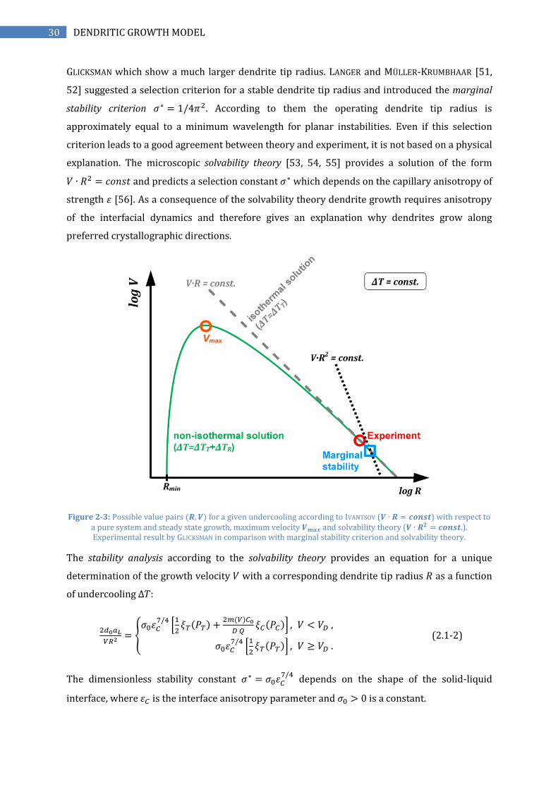
Figure 2-3: Possible value pairs (𝑹, 𝑽) for a given undercooling according to IVANTSOV (𝑽 ∙ 𝑹 = 𝒄𝒐𝒏𝒔𝒕) with respect to a pure system and steady state growth, maximum velocity 𝑽𝒎𝒂𝒙 and solvability theory (𝑽 ∙ 𝑹𝟐 = 𝒄𝒐𝒏𝒔𝒕.). Experimental result by GLICKSMAN in comparison with marginal stability criterion and solvability theory.
The stability analysis according to the solvability theory provides an equation for a unique
determination of the growth velocity 𝑉 with a corresponding dendrite tip radius 𝑅 as a function
of undercooling ∆𝑇:
2𝑑0𝑎𝐿
𝑉𝑅2= {
𝜎0휀𝐶7/4[1
2𝜉𝑇(𝑃𝑇) +
2𝑚(𝑉)𝐶0
𝐷 𝑄𝜉𝐶(𝑃𝐶)] , 𝑉 < 𝑉𝐷 ,
𝜎0휀𝐶7/4[1
2𝜉𝑇(𝑃𝑇)] , 𝑉 ≥ 𝑉𝐷 .
(2.1-2)
The dimensionless stability constant 𝜎∗ = 𝜎0휀𝐶7/4
depends on the shape of the solid-liquid
interface, where 휀𝐶 is the interface anisotropy parameter and 𝜎0 > 0 is a constant.
31 DENDRITIC GROWTH MODEL
𝜎∗ = {
2𝑑0𝑎𝐿𝑉𝑅2
=1
4𝜋2≈ 0.0253 (planar phase boundary)
0.0192 (spherical phase boundary)0.025 (parabolic phase boundary)
𝜉𝑇(𝑃𝑇) and 𝜉𝐶(𝑃𝐶) are the stability functions which depend on the thermal and the chemical
PÉCLET numbers. They are given by:
𝜉𝑇(𝑃𝑇) =1
(1 + 𝑎112⁄ 𝑃𝑇)
2 ,
𝜉𝐶(𝑃𝐶) =1
(1 + 𝑎212⁄ 𝑃𝐶)
2 ,
where = 15𝐶 is the stiffness for a crystal with cubic symmetry and the anisotropy 𝐶 of the
interfacial energy. In particular, 𝜉𝑇.𝐶(𝑃𝑇,𝐶) → 1 for small growth velocities (𝑉 → 0) and
𝜉𝑇.𝐶(𝑃𝑇,𝐶) → 0 for high growth velocities (𝑉 → ∞). The parameters 𝑎1 and 𝑎2 are obtained by
fitting to experimental data or by an asymptotical analysis [57].
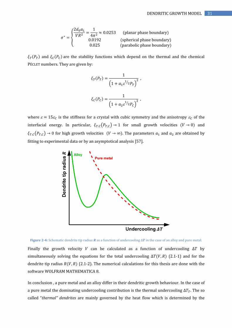
Figure 2-4: Schematic dendrite tip radius 𝑹 as a function of undercooling ∆𝑻 in the case of an alloy and pure metal.
Finally the growth velocity 𝑉 can be calculated as a function of undercooling ∆𝑇 by
simultaneously solving the equations for the total undercooling ∆𝑇(𝑉, 𝑅) (2.1-1) and for the
dendrite tip radius 𝑅(𝑉, 𝑅) (2.1-2). The numerical calculations for this thesis are done with the
software WOLFRAM MATHEMATICA 8.
In conclusion , a pure metal and an alloy differ in their dendritic growth behaviour. In the case of
a pure metal the dominating undercooling contribution is the thermal undercooling ∆𝑇𝑇. The so
called “thermal” dendrites are mainly governed by the heat flow which is determined by the

32 DENDRITIC GROWTH MODEL
thermal diffusivity 𝐷𝑇 ≈ 10−5 𝑚2/𝑠. On the contrary for an alloy the constitutional undercooling
∆𝑇𝐶 dominates for low undercoolings. The so called “solutal” dendrites are governed by mass
diffusion which is determined by the diffusion coefficient 𝐷𝐶 ≈ 10−9 𝑚2/𝑠. “Thermal” dendrites
are much faster as “sulutal” dendrites because 𝐷𝑇 and 𝐷𝐶 differ by four orders of magnitude. At
large undercoolings a transition occurs from sulutal-controlled to thermally-controlled dendrite
growth. At high growth velocities (large undercoolings) an alloy behaves like a pure metal.
2.2 Influence of Convection on Dendrite Growth
So far we treated dendritic solidification as a steady state one-dimensional sharp interface
process which is an interplay between heat/mass transport, attachment kinetics and surface
energy. However experimental reality cannot provide ideal conditions like for instance a resting
liquid in its mechanical equilibrium without fluid flow. In experiments, natural and forced
convection occur. Namely fluid flow is generated by BUOYANCY forces due to thermal and/or
concentrational gradients (natural convection), by surface tension gradients (MARANGONI
convection), and by external forces like electromagnetic stirring (forced convection). In
particular, the fluid flow acts on the concentration and temperature gradient field ahead of the
solidification front which will be discussed in the following and implemented into the sharp
interface model.
Figure 2-5: Left image: Effect of fluid flow on the growth of a settling NH4Cl crystal showing an enhanced growth velocity in the opposing fluid flow direction [10]. Right image: Computed streamtraces for fluid flow over a phase-
field modelled growing isolated dendrite [58].
The left image of Figure 2-5 shows a settling NH4Cl growing dendritic crystal which corresponds
to an upward fluid flow 𝑈 [10]. A significant enhanced dendrite growth velocity can be observed
in the opposite direction of the fluid flow relative to the crystal. The right image shows a phase-
field simulation of a growing dendrite with indicated fluid flow streamtraces [58]. Obviously the
dendrite grows faster against the direction of fluid flow 𝑈.

33 DENDRITIC GROWTH MODEL
Consequently the mechanism of convection inside the undercooled melt has to be taken into
account to model the experimental results. We will see later, especially if the fluid flow velocity
is in the same order of magnitude or greater as the solidification velocity itself. A modification to
the LKT-model with respect to the effect of forced convection caused by electromagnetic stirring
has been suggested by GALENKO et al. [59, 60].
As an estimation for electromagnetic levitation experiments (experimental method described in
chapter 4.1), the fluid flow velocity 𝑈0 is assumed to be a result of the balance between the
electromagnetic field, gravitation, and the viscous dissipation:
𝑈0 =
[ 2
𝜌
(
𝜌𝑔𝑅0 +
𝐵02 (1 − 𝑒𝑥𝑝 (2
𝑅0𝛿⁄ ))
8𝜋+𝜌𝜂2
2𝛿2
)
]
12⁄
,
where 𝑔 is the gravity acceleration, 𝜌 is the mass density, 𝜂 is the dynamic viscosity of the liquid,
𝛿 is the skin depth, 𝑅0 is the radius of the sample, and 𝐵0 is the time averaged value of the
magnetic field inside the levitation coil.
Figure 2-6: Upwards growing dendrite in an electromagnetic levitated liquid sample with indicated streamlines. In this idealized case the fluid flow velocity 𝑼𝟎 occurs in the opposite direction as the dendrite growth velocity 𝑽.
In the case of forced convection inside the melt, the stability parameter 𝜎∗ becomes dependent
on the fluid flow velocity 𝑈0 which can be expressed by:
𝜎∗ =𝜎0휀𝑐
74⁄
1 + 𝜒(𝑅𝑒)𝑈0 𝛤𝑎 ∆𝑇ℎ𝑦𝑝
,
where 𝜎0 is the stability constant, 𝑅𝑒 is the REYNOLDS number and 𝜒(𝑅𝑒) is a function which is
defined by BOUISSOU and PELCÉ in Ref. [61]. The stability parameter 𝜎∗ was chosen to fulfil
𝜎0휀𝑐7 4⁄ 𝜎∗⁄ = 1.675 as a result of phase-field modelling [58] in the idealized case of an upstream
fluid flow for a free growing dendrite which is illustrated in Figure 2-6. The thermal

34 DENDRITIC GROWTH MODEL
undercooling ∆𝑇𝑇 and the constitutional undercooling ∆𝑇𝐶 have to be modified due to
convection. This is expressed by additional thermal and mass diffusion PÉCLET numbers which
dependent on the fluid flow velocity 𝑈0 which are defined by:
𝑃𝑇𝑓(𝑈0, 𝑅) =
𝑈0 ∙ 𝑅
2𝑎𝐿,
𝑃𝐶𝑓(𝑈0, 𝑅) =
𝑈0 ∙ 𝑅
2𝐷.
Consequently the thermal undercooling ∆𝑇 = 𝑇𝑖 − 𝑇𝐿∞ is given by:
∆𝑇𝑇 = 𝑇𝑖 − 𝑇𝐿∞ = ∆𝑇ℎ𝑦𝑝 ∙ 𝑃𝑇 ∙ 𝑒𝑥𝑝(𝑃𝑇 + 𝑃𝑇
𝑓)∫ 𝑞−1 exp(−𝑞 ∙ 𝑃𝑇 + (𝑙𝑛 𝑞 − 𝑞)𝑃𝑇
𝑓)𝑑𝑞
∞
1
,
and the constitutional undercooling ∆𝑇𝐶 changes to:
∆𝑇𝐶 =𝑚𝑉𝐶0(𝑘𝑉 − 1)𝐼𝑣
𝑓(𝑃𝐶 , 𝑃𝐶𝑓)
1 − (1 − 𝑘𝑉)𝐼𝑣𝑓(𝑃𝐶 , 𝑃𝐶
𝑓) ,
while 𝐼𝑣𝑓(𝑃𝐶 , 𝑃𝐶𝑓) = 𝑃𝐶 ∙ 𝑒𝑥𝑝(𝑃𝐶 + 𝑃𝐶
𝑓)𝐸1−𝑃𝐶
𝑓(𝑃𝐶 + 𝑃𝐶𝑓) is a modified IVANTSOV function.

35 EUTECTIC GROWTH MODEL
3 EUTECTIC GROWTH MODEL
The dendritic growth is a single-phase growth mechanism. Eutectic growth is a cooperative
growth of two solid phases within one liquid phase. This chapter gives a description of the
eutectic growth theory and introduces a modified JACKSON-HUNT model [62] for eutectic
solidification to analyse the experimental results. For further details and explanations the author
refers to Chapter 7 in the book METASTABLE SOLIDS FROM UNDERCOOLED MELTS by D.M.
HERLACH, P. GALENKO and D. HOLLAND-MORITZ [11].
The Fe-B system is a metallic glass former. Metallic glasses are characterized by the fact that no
crystallographic long range order is present in the solidified material. For instance, if the Fe-17
at.% B alloy melt is undercooled to the glass transition temperature 𝑇𝑔 the undercooled melt
freezes into a metastable amorphous phase. However, this experimental conditions cannot be
realized by the experimental methods used within this thesis. Therefore much higher cooling
rates are necessary (~ 106 𝐾 𝑠−1). In the case of 1g-EML experiments which are performed in
this work, the Fe-17 at.% B alloy solidifies eutectic. The eutectic solidification is a cooperative
growth of two phases simultaneously which is shown schematically in Figure 3-1. In particular,
𝛾-Fe solid solution and stoichiometric compound 𝐹𝑒2𝐵 solidify.
Figure 3-1: Schematic illustration of eutectic solidification in Fe-B alloy system. λ is the interlamellar spacing. 𝑺𝜸 and
𝑺𝑭𝒆𝟐𝑩 are the half widths of 𝜸-Fe and Fe2B. 𝝈𝜸/𝑳, 𝝈𝑭𝒆𝟐𝑩/𝑳 and 𝝈𝜸/𝑭𝒆𝟐𝑩 are the interface energies at the triple junction
point (TJ). 𝑽 is the steady state growth velocity of both phases solidifying cooperatively into the liquid.

36 EUTECTIC GROWTH MODEL
In cooperation with Professor HAIFENG WANG and his student KUANG WANGWANG a modified
JACKSON-HUNT model [62] for eutectic solidification is used within this thesis to model the 1g-
EML experimental results for the eutectic composition Fe-17 at.% B [63].
Eutectic alloys have been studied intensively by experiments and modelling due to their
economic importance (e.g. casting [64], pattern formation and selection [65]). The pioneering
work for modelling eutectic growth was done by JACKSON and HUNT (JH) in 1966 [62]. They
assumed a linear phase-diagram (LPD) for solidification under local equilibrium conditions. The
JH model is able to predict the experimental results in directional solidification (e.g. Al-Cu [66]
and In–In2Bi [67] eutectic alloys). In order to show some physical insights into rapid
solidification, two simple types of LPD were adopted by TRIVEDI-MAGNIN-KURZ (TMK) [68]. One
model assumes cigar-shaped growth with parallel liquidus and solidus lines below the
equilibrium eutectic temperature while the other model uses constant and equal partition
coefficients. Subsequently, non-equilibrium kinetics are implemented with LPD to apply for
rapid solidification in a dilute alloy [69].
Even though TMK-kind models [68, 69] are widely used in rapid solidification, the LPDs are
rarely found in practical alloy systems. In fact, the assumption of dilute alloys with LPD is only
applicable to small undercooling [70, 71]. In the case of an undercooled eutectic alloy, the
negative temperature gradient ahead of the migrating interface results in an interface instability
which leads to the formation of an eutectic dendrite morphology [72, 73]. Assuming a purely
thermal driven dendrite, the eutectic growth model (e.g. TMK [68]) and dendrite growth model
(e.g. Lipton-Kurz-Trivedi (LKT) [46]) can be combined to describe the solute diffusion parallel to
the interface, and the thermal diffusion perpendicular to it [74, 75]. However these eutectic
dendrite growth models for dilute alloys with LPD [74, 75] cannot predict the experimental
results, especially at high undercooling according to calculation results in Refs. [46, 73, 74].
Therefore a modified model with non-linear phase diagram (NLPD) is introduced in the
following.
37 EUTECTIC GROWTH MODEL
3.1 Current Model for Concentrated Alloys with Non-Linear Phase Diagram (NLPD)
Figure 3-1 illustrates the concept of eutectic solidification and shows the used important
variables. For a migrating planar interface under steady state conditions, the non-equilibrium
diffusion equation is given by [76]:
2 22
2 2 21 0L L L
LDL
C C CV V
D ZX V Z
(3.1-1)
The solution of Eq. (3.1-1) in the case of lamellar eutectic growth is [76]:
0 2 2
0
0
cos exp ,, 1
,
n
n n DL
nL L DL
DL
VZC B b X V V
C X Z D V V
C V V
(3.1-2)
Here LC is the liquid concentration,
0C is the liquid concentration far from the interface, V is
the growth velocity, DLV is the solute diffusion velocity in the liquid,
LD is the solute diffusion
coefficient, 2nb n ( 0,1,2,......n ) and 2
1 1 2 2n en P
with the lamellar spacing and
2e LP V D the PÉCLET number.
In order to obtain the Fourier coefficients nB ( 0,1,2,......n ), the average mass conservation law
at the interface is introduced by [77]:
0
, 0
,
LL L
LZ
C C X SD C
C C S X S SV Z
2 2 2Fe B Fe B Fe B
, (3.1-3)
where S ( S2Fe B ) is the half width of the -Fe ( 2Fe B ) lamellar spacing, C
is the average solute
concentration of at the L interface, C2Fe B the concentration of a stoichiometric compound
2Fe B is constant and equal to 1 3 and, *
LC and *
LC2Fe B are the average liquid concentration at the
L and the L2Fe B interface which can be obtained from Equation (3.1-2) as:
*
0 00
1
1,0 sin
fn
L L
n
BC C X dX C B n f
f n f
(3.1-4)
*
0 0
1
1,0 sinn
L Lf
n
BC C X dX C B n f
f n f
2
2 2
Fe B
Fe B Fe B
(3.1-5)
Substituting equations (3.1-2), (3.1-4) and (3.1-5) into equation (3.1-3) and noting that the
concentration at the triple-junction point (e.g. X S , 0Z ) is equal to the kinetic eutectic
concentration LC of a planar interface [77, 78], the Fourier coefficients nB are obtained as:

38 EUTECTIC GROWTH MODEL
0 0
1
cosL n
n
B C C B n f
(3.1-6)
2
2
2
Fe B 2 21 Fe B
2sin2sin/ 1n
mn m
m fn fB C C
n m f f
( 1n ), (3.1-7)
where f and 2Fe Bf are the volume fraction of -Fe and
2Fe B , respectively. The introduction of
an average mass conservation law with the interface equation (3.1-3) instead of the mass
conservation law at the interface for dilute alloys with LPD, makes the current solution of
diffusion equation applicable to concentrated alloys with NLPD [77, 78].
The kinetic eutectic composition LC is determined by the kinetic conditions at the L
(equations (3.1-8) and (3.1-9)) and 2Fe B L (equation (3.1-10)) interfaces:
1 Fe^ B^^ 2
^ ^ ^ 21 1 exp
L Lg I L
I
g IDL L L DL
R TV V
R TV C C C V
, (3.1-8)
^ B^ ^ Fe^
0
11 exp
L L L L
g I
C CV
V R T
, (3.1-9)
2 2 2 2 2 2
12
^ B^ Fe^^Fe B Fe B Fe B Fe B Fe B Fe B
^2 20
111 exp
1
L L LL
g ILDI DL
C C C C gV
V R TCV V V
, (3.1-10)
where I
DLV is the interfacial solute diffusion velocity, 0V is the upper limit velocity of V ,
^ ^ ^j j j
i L i L ( i , 2Fe B ; Fej , B ) is the chemical potential difference between solid and
liquid, ^ B^ Fe^
L L L is the solute diffusion potential, gR is the gas constant,
IT is the interface
temperature and 2Fe Bg the Gibbs energy of
2Fe B which is temperature-dependent but not
concentration-dependent. For the solid-solution phase -Fe, there are two independent
dissipative processes which are a trans-interface diffusion equation (3.1-8) and an interface
migration equation (3.1-9). Whereas for the stoichiometric compound 2Fe B two dissipative
processes dependent on each other and the kinetic interface condition is given by only one
equation (3.1-10) [78, 79].
In the case of LPD, the average interface undercooling is adopted generally to obtain uniquely
the relation between and ∆𝑇 ( e
E IT T ) for a given growth velocity V from the minimum
undercooling principle 0IT [62]. However this method is not applicable here because the
interface undercooling contributions (e.g. constitutional undercooling, curvature undercooling
etc.) cannot be obtained analytically in the case of NLPD [78, 79, 80]. Therefore, the average

39 EUTECTIC GROWTH MODEL
kinetic interface conditions for migration of the L and 2Fe B L interfaces are averaged by the
volume fractions of and 2Fe B :
2 2 2 2 2 2 2 2 2
2
* B* * Fe*
/ /
0
12
* B* Fe*^Fe B Fe B Fe B Fe B Fe B Fe B Fe B Fe B/ Fe B/
*2 20 Fe B
11 exp
111 exp
1
L L L L m L L
g I
L L L m L LL
L g IDI DL
C C V KV f V
R T
C C C C g V Kf
V C R TV V V
(3.1-11)
where 2sini L i iK f with i ( i and
2Fe B ) the contact angle is the average interface
curvature [80], / L and 2Fe B/ L are the interface energies.
mV is the molar volume which is
assumed to be the same for 𝛾-Fe and Fe2B. Similarly, the averaged kinetic interface condition for
trans-interface diffusion at the L interface is:
1 * ** 2
* * * 21 1 exp
A B
L Lg I L
I
g IDL L L DL
R TV V
R TV C C C V
. (3.1-12)
So far, a model for lamellar eutectic growth under steady-state conditions is proposed by
adopting the interface kinetic models for concentrated alloys [79, 80] (i.e. equations (3.1-8)-(3.1-
12)). The next step is to impose a negative temperature gradient for the growing lamellar
eutectic interface in order to generate its instability concerning a eutectic dendrite. In the case of
such purely thermal-controlled dendrite growth [74, 75], the thermal undercooling TT can be
obtained from the IVANTSOV solution [81] as:
f
T TL
P
HT Iv P
C
, (3.1-13)
where fH ( f ff H f H
) is the average latent heat of fusion, L
PC ( L L
P Pf C f C
) is the
average specific heat of undercooled melts, 2T LP VR with L the thermal diffusion coefficient
and R the dendrite tip radius is the thermal PÉCLET number. Equation (3.1-13) gives actually a
relation between VR and TT . To find a unique solution, a second equation from the solvability
theory [82, 83] is needed:
7/4
0
/ 2/ L
T f T PR P H C
, (3.1-14)
where 21 1T T Ta P is a stability function , L Lf f is the average GIBBS-THOMSON
coefficient while i
Li i L m fV S and i
fS is the average entropy of fusion of the i L interface,

40 EUTECTIC GROWTH MODEL
is the anisotropy coefficient, 0 1 0.42 the stability constant, and 0.3Ta . For a given velocity
V , R and TT are determined by equations (3.1-13) and (3.1-14).
The described combination of the lamellar eutectic model and the thermal dendrite growth
model defines a total undercooling I TT T T . Consequently, , R and T can be calculated
for a given growth velocity V with the current eutectic dendrite growth model for concentrated
alloys with NLPD (i.e. Eqs. (3.1-4)-(3.1-14)).
3.2 Model of Li and Zhou (LZ) for Dilute Alloys with Linear Phase-Diagram (LPD)
In the LI and ZHOU model (LZ) model for dilute alloys with linear phase diagram (LPD) [75], the
TRIVEDI-MAGNIN-KURZ (TMK) model [68] is used to describe the lamellar eutectic growth. A
second type of LPD in the TMK-model is introduced with constant and equal equilibrium
partition coefficients ek , which is a good approximation for the Fe-B eutectic alloy. The relations
between the interface undercooling IT , the growth velocity V and the lamellar spacing is
given by the minimum undercooling principle [76, 69]:
2 1
2
KV
K , (3.2-1)
1L L
I
L L
m m PT
m m P P
2
2
Fe B
Fe B
, (3.2-2)
where
1
sinsin2
LL
L L
Kf m f m
2 2
2 2
Fe B Fe B
Fe B Fe B
, (3.2-3)
2
1
L
kK P P
f f D
2Fe B
, (3.2-4)
3
2
21
1sin
1 1 2
n
nn
pP n f
n p k
, (3.2-5)
23
2
2 21
1sin
1 1 1
n n
nn n
p pP P n f
n p p
. (3.2-6)
Here 2n ep n P , 2 21 DLV V , k is the velocity-dependent non-equilibrium partition
coefficient, Lm and Lm2Fe B are the slopes of kinetic liquidus which are given by [82, 83]:

41 EUTECTIC GROWTH MODEL
e
I
DL
I
DL
Vk
Vk k k
V
V
2Fe B
, (3.2-7)
2
1 ln 11
e
Li
Li e e
D
m k Vm k k
Vk k
(𝑖 = 𝛾, 𝐹𝑒2𝐵) . (3.2-8)
The combination of equations (3.2-1)-(3.2-8) together with the thermal dendrite growth model
(3.1-13) and (3.1-14) lead to the LZ eutectic dendrite growth model for dilute alloys with LPD. In
particular, the LZ model [75] is extended by taking into account non-equilibrium solute diffusion
( in equations (3.2-5)-(3.2-7)) and non-equilibrium interface kinetics (equations (3.2-7) and
equations (3.2-8)). To put it more simply, the only difference between the current and the LZ
model is whether dilute alloys with LPD are assumed or not.
3.3 Kinetic Liquidus Slopes for Large Undercoolings
Figure 3-2 shows the evolutions of equilibrium (kinetic) liquidus slopes e
Lm and 2Fe B
e
Lm ( Lm and
2Fe BLm ) as a function of undercooling T for the presented model of concentrated alloys with
NLPD. An interesting result for the -Fe phase at high undercoolings is the fact that the kinetic
liquidus slope Lm becomes smaller as the equilibrium liquidus slope 2Fe B
e
Lm .
Figure 3-2: Evolution of equilibrium and kinetic liquidus slopes as a function of undercooling.

42 EUTECTIC GROWTH MODEL
Figure 3-3: Kinetic phase-diagram of the eutectic Fe-B sytem in the case of concentrated alloys with NLPD (a) and dilute alloys with LPD (b).
Figure 3-3 shows the kinetic phase-diagram for the eutectic Fe-B alloy system in the case of
concentrated alloys with NLPD (a) and dilute alloys with LPD (b). In the case of a given
composition for concentrated alloys with NLPD, the kinetic liquidus of -Fe and Fe2B decreases
while the kinetic solidus of -Fe increases with the growth velocity V . For the stoichiometric
compound Fe2B occurs no solute trapping [78, 80] while the kinetic and equilibrium solidus
coincide with each other. For a given low temperature (or high undercooling), e.g. 1200T K ,
Lm decreases continuously from e
Lm as the increase of V and thus Lm is smaller than e
Lm
(tangents in Figure 3-3(a)). If both -Fe and Fe2B are assumed as dilute alloys, their kinetic
(a)
(b)

43 EUTECTIC GROWTH MODEL
liquidus for a given concentration decrease while their kinetic solidus increase with growth
velocity V (Figure 3-3(b)). Lm (2Fe BLm ) thus is always larger than e
Lm (2Fe B
e
Lm ). Furthermore the
smaller slope of kinetic liquidus at high undercooling implies the importance to extend the
eutectic theory to concentrated alloys with NLPD.

44 EUTECTIC GROWTH MODEL

45 EXPERIMENTAL METHODS
4 EXPERIMENTAL METHODS
This chapter explains the experimental methods to study rapid solidification for deep
undercoolings. Most experiments are performed in a terrestrial electromagnetic levitator (1g-
EML) which is shown in Figure 4-1. In order to investigate and reduce convectional effects some
experiments were done in the TEMPUS1 facility (µg-EML) under reduced gravity conditions
during parabolic flight. Furthermore to vary fluid flow conditions, experiments were performed
in a melt fluxing facility under influence of a high strength static magnetic field up to 6 𝑇.
In addition, experiments with an infrared camera were performed as a feasibility study. This is
especially interesting for low undercoolings (∆𝑇 < 50 𝐾) and low melting materials. Due to the
maximum framerate of 850 𝑓𝑝𝑠 the investigated growth velocities are limited to about 1 𝑚/𝑠.
The Microstructure of the as solidified samples is analysed with a scanning electron microscope
(SEM) and Electron Backscatter Diffraction (EBSD) in order to examine the dendritic and
eutectic structure including its crystallographic orientation.
Figure 4-1: The photo shows a freely floating liquid iron sample at a temperature of about 𝟏𝟔𝟎𝟎 °𝑪. A water-cooled copper coil generates a high-frequency magnetic field, in which a seven-millimetre iron droplet levitates.
4.1 Electromagnetic Levitation (1g-EML)
The electromagnetic levitation (EML) technique [3] is an experimental method to deeply
undercool electrically conductive materials (e.g. metallic melts) far below their equilibrium
melting temperature and allows direct observation (in-situ) of the solidification process. Even
highly reactive materials can be processed. This containerless technique makes it possible to
avoid heterogeneous nucleation on container walls. By the use of high purity materials under
1 Tiegelfreies Elektro-Magnetisches Prozessieren unter Schwerelosigkeit (TEMPUS)

46 EXPERIMENTAL METHODS
clean environmental conditions it is possible to reach deep undercoolings up to 300 𝐾 prior to
solidification. The vacuum-chamber is evacuated to 10−7 𝑚𝑏𝑎𝑟 and backfilled with high-purity
helium (6N) to a few hundred 𝑚𝑏𝑎𝑟 in order to limit evaporation of the sample. The
transformation process of the undercooled liquid phase into the solid phase leads to a visible
contrast between solid and liquid due to the release of latent heat during rapid solidification.
The advancement of the solidification front is recorded by a high-speed video camera. Figure 4-2
shows schematically an EML experimental setup. The facility consists of a water-cooled copper
levitation coil which creates an alternating magnetic field due to an alternating current 𝐼
(≈ 400 𝐴) and high voltage (≈ 100 𝑉) at high frequency (up to 300 𝑘𝐻𝑧). The resulting
magnetic field amplitude 𝐻0 is about 105 𝐴/𝑚. In general, a high frequency magnetic field
induces an eddy (current) field an electrically conducting sample. Particularly, the magnetic field
induces a voltage 𝑈𝑖𝑛𝑑~𝑓 ∙ 𝐻0 and an eddy current 𝑗𝑖𝑛𝑑~𝜎 ∙ 𝑓 ∙ 𝐻0 in the metallic sample with the
electric conductivity 𝜎. The interaction between the sample and the magnetic field can be
described as followed. To consider the MAXWELL equations, a temporal variation of a magnetic
field – 𝜕�⃗� 𝜕𝑡⁄ = ∇⃗⃗ × �⃗� induces eddy currents in the sample which react back on the source of the
magnetic field (LENZ’s law) and create a magnetic field which is counter directed to the primary
field. That results in a repulsive LORENTZ force 𝐹𝐿⃗⃗⃗⃗ = −∇⃗⃗ (�⃗⃗� ∙ �⃗� ) between the levitation coil and
the sample, where �⃗⃗� is the magnetic dipole moment induced in the sample. In other words, the
sample behaves like a diamagnet and is repelled by the coil. The LORENTZ force acts on each point
of the sample surface, while it is zero at the north and south pole. In the case of a levitating
sample, the LORENTZ force is sufficient to compensate the gravitational force 𝐹𝐺⃗⃗⃗⃗ = 𝑚 ∙ 𝑔 , where
𝑚 is the mass of the sample and 𝑔 is the gravitational acceleration. The levitated sample can be
assumed as a droplet-like head of liquid which is hold mainly on its equator at the surface where
the LORENTZ force is strongest. Stable levitation conditions depend on the coil geometry and
sample properties (like electrical conductivity, diameter and mass). It should be mentioned, that
as a side effect of the strong electromagnetic field which is necessary for lifting the sample
against gravity, strong electromagnetic stirring is applied. This forced convection results in fluid
flow velocities up to 0.3 𝑚/𝑠 [9] in the liquid sample.

47 EXPERIMENTAL METHODS
Figure 4-2: Schematic view of an electromagnetic levitation facility. The sample is processed under noble gas
atmosphere in a vacuum chamber. Levitation and heating are achieved by an electromagnetic field produced by high
frequency alternating currents flowing through a water-cooled copper coil. The actual force which lifts the sample
against gravity 𝑭𝑮 is the LORENTZ-force 𝑭𝑳 which acts mainly at the equator on the surface. The temperature is
measured contactless with an infrared-pyrometer.
The electromagnetic levitation and inductive heating are coupled and appear simultaneously in
EML. The levitation force is proportional to 𝑗𝑖𝑛𝑑 ∙ 𝐻0 whereas the power of absorption
𝑃𝑂ℎ𝑚 = 𝑈𝑖𝑛𝑑 ∙ 𝑗𝑖𝑛𝑑 is proportional to 𝐻02. In order to achieve an experimental optimization for
levitation and inductive heating, the amplitude of the coil current and the sample mass can be
adjusted.
Samples for an EML experiment are about 1 𝑔 in weight and 6 − 7 𝑚𝑚 in diameter. The
temperature is measured contactless at the top of each sample by a two-color pyrometer with a
sampling rate of 100 𝐻𝑧. The accuracy of the pyrometer is approximately ±3 𝐾. The emissivity 휀
of the sample material is unknown. Using the pyrometer at a constant emissivity 휀 of 0.2
requires a correction of the measured temperature values 𝑇𝑝𝑦𝑟 . A temperature 𝑇 can be
calculated by using following equation:
1
𝑇=
1
𝑇𝑝𝑦𝑟+1
𝑇𝐿−
1
𝑇𝐿𝑝𝑦𝑟 ,
where 𝑇𝑝𝑦𝑟 is the temperature recorderd by the pyrometer, 𝑇𝐿𝑝𝑦𝑟
is the measured liquid
temperature by the pyrometer and 𝑇𝐿 is the liquidus temperature taken from the literature

48 EXPERIMENTAL METHODS
phase diagram. The corrected temperatures can be calculated and the undercooling ∆𝑇 can be
extracted from the temperature time profile.
Figure 4-3: Schematic temperature-time profile measured in an undercooling electromagnetic levitation experiment.
First the sample levitates in solid state, followed by melting, overheating in liquid state, undercooling until rapid
solidification (recalescence) occurs spontaneously with dendritic growth, solidification of residual liquid, and ends up
in solid state again.
Figure 4-3 shows a schematic temperature-time profile for a typical undercooling experiment.
The solid sample is levitated and at the same time inductively heated. By increasing the power
the sample starts to melt. Once the sample is completely molten the temperature increases
rapidly. This point in the temperature-time profile is used as a reference for the liquidus point
for calibrating the temperature measured by the pyrometer. Overheating is applied to get rid of
pollutions and potential oxide layers. The sample is cooled by reducing the power to a minimum
and additionally by a diffuse He-gas flow. While the sample is undercooled spontaneous
nucleation takes place. A primarily formed crystal nucleus grows rapidly and during subsequent
growth latent heat is released. During this recalescence a contrast is visible between the dark
undercooled liquid and bright solidified material which can be recorded by a high-speed camera.
After recalescence a portion of the sample is solidified into a dendritic network. These dendrites
thicken until the residual liquid solidifies.
4.2 Electromagnetic Levitation under Reduced Gravity (µg-EML)
Concerning terrestrial EML, the electromagnetic field necessary for levitation induces strong
convective fluid flow inside the melt due to electromagnetic stirring. The resulting fluid flow
velocity in 1g-EML is estimated to be around 0.3 m/s [9]. In order to verify the influence of
convection on the growth velocity and morphology, experiments were performed under reduced
gravity conditions in micro-gravity (µg) during parabolic flight missions using the TEMPUS2
facility [84] aboard an AIRBUS A300 Zero-G airplane (cf. Figure 4-4). The experimental setup of
2 Tiegelfreies Elektro-Magnetisches Prozessieren unter Schwerelosigkeit (TEMPUS)

49 EXPERIMENTAL METHODS
an µg-EML is similar to the 1g-EML. The main difference in the TEMPUS facility compared to
terrestrial EML is the decoupling of positioning and heating due to superposition of a weak
quadrupole positioning field (150 kHz) and a strong dipole heating field (400 kHz). During
solidification the dipole heating field is turned off, resulting in a low remaining fluid flow
velocity of about 0.05 m/s [9] and therefore one order of magnitude lower as in terrestrial 1g-
EML.
Figure 4-4: Left image: TEMPUS facility for containerless electromagnetic levitation. Right image: AIRBUS A300 Zero-G airplane by NOVESPACE [85].
To achieve micro-gravity for about 22 𝑠 the airplane follows a parabolic flight manoeuvre which
is shown schematically in Figure 4-5. The aircraft initially climbs up at an angle of 47 degrees
(injection point) following a parabolic trajectory until the pilot pulls out the nose with an angle
of 42 degrees downwards (recovery point). Under these circumstances the remaining
acceleration forces are in the order of 10−3 𝑔 during 22 𝑠 of reduced gravity. The parabolic flight
campaigns are performed by the company NOVESPACE from Bordeaux, France.
Figure 4-5: Schematic view of a parabolic flight manoeuvre

50 EXPERIMENTAL METHODS
The TEMPUS facility was already flown three times aboard Space Shuttle Spacelab missions
(IML-2, MSL-1 and MSL-1R), five sounding rocket flights with the carrier TEXUS3, and more than
2000 parabolas during several parabolic flight campaigns. Since September 2014 an EML is also
installed at the International Space Station (ISS). The Fe-10 at.% B alloy was qualified within this
thesis due to a parabolic flight experiment to be a sample for batch 2 in 2015/16 aboard the ISS
as part of the MAGNEPHAS project.
Figure 4-6: German astronaut ALEXANDER GERST installing and switching on the EML-ISS (picture by ESA4 [86]) in Nov. 2014 aboard the International Space Station (picture by NASA5 [87]).
3 Technologische Experimente unter Schwerelosigkeit (TEXUS) 4 European Space Agency (ESA) 5 National Aeronautics and Space Administration (NASA)

51 EXPERIMENTAL METHODS
4.3 Melt-Fluxing in a Static Magnetic Field (MF)
Beside 1g-EML and µg-EML it is possible to achieve different fluid flow conditions by using a
strong magnetic field. A static magnetic field reduces the fluid flow due to magnetic damping in
conductive materials which could be shown by YASUDA et al. [88].
In 1939 BARDENHEUER and BLECKMANN published first melt fluxing experiments (MF) of
undercooling Fe and Ni bulk melts. With this technique they were able to undercool samples to
about ∆𝑇/∆𝑇𝐸 ≈ 0.18. Later on, TURNBULL et al. [89] produced an amorphous Pd40Ni40P20 sphere
after fluxing the melt in B2O3 with cooling rates of just a few 𝐾/𝑠. In 1987, FLEMINGS et al. [90]
combined the MF with the EML technique and investigated dendritic growth of undercooled Ni-
Sn alloys.
YECKEL and DERBY did three-dimensional simulations of the flow induced by transient
acceleration (g-jitter) in microgravity crystal growth [91]. In most cases, the application of a
magnetic field suppresses flow oscillations, but for transverse jitter at intermediate frequencies,
flow oscillations are increased.
ZHANG et al. combined EML with a superconducting magnet [92]. They could show by
investigations of Co-Cu alloys which show a metastable miscibility gap that the effect of a static
magnetic field of 2 𝑇 is similar to that of reduced gravity during parabolic flights.
The melt fluxing experiments in a static magnetic field for this work were performed together
with Professor Dr. JIANRONG GAO at the Key Laboratory on Electromagnetic Processing of Materials
of the North-Eastern University (Shenyang, China). A static magnetic field was applied with a
superconducting magnet up to 6 𝑇. Figure 4-7 shows the experimental setup. The sample is
covered with melt flux on an Al2O3 sample holder. The temperature is measured by an infrared-
pyrometer while the solidification is recorded by a high-speed video camera (HSC) with a
telelens and prism. Due to the high magnetic field the HSC has to be placed at a safe distance
which leads to a low resolution of the videos to about 64 × 64 𝑝𝑥 corresponding to a sample
diameter of about 7 𝑚𝑚.
B2O3, DURAN and PYREX are used as fluxing agents due to their ability of high solubility for
metal oxides at high temperatures. Those materials act as impurity absorber.

52 EXPERIMENTAL METHODS
Figure 4-7: Schematic experimental setup for melt fluxing experiments in a static magnetic field produced by a superconducting magnet. The estimated flow field inside the liquid sample is indicated as stream lines.
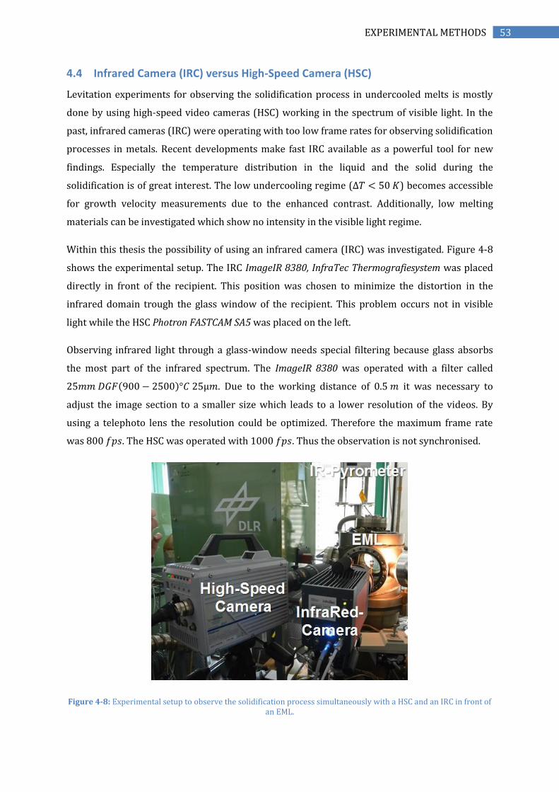
53 EXPERIMENTAL METHODS
4.4 Infrared Camera (IRC) versus High-Speed Camera (HSC)
Levitation experiments for observing the solidification process in undercooled melts is mostly
done by using high-speed video cameras (HSC) working in the spectrum of visible light. In the
past, infrared cameras (IRC) were operating with too low frame rates for observing solidification
processes in metals. Recent developments make fast IRC available as a powerful tool for new
findings. Especially the temperature distribution in the liquid and the solid during the
solidification is of great interest. The low undercooling regime (∆𝑇 < 50 𝐾) becomes accessible
for growth velocity measurements due to the enhanced contrast. Additionally, low melting
materials can be investigated which show no intensity in the visible light regime.
Within this thesis the possibility of using an infrared camera (IRC) was investigated. Figure 4-8
shows the experimental setup. The IRC ImageIR 8380, InfraTec Thermografiesystem was placed
directly in front of the recipient. This position was chosen to minimize the distortion in the
infrared domain trough the glass window of the recipient. This problem occurs not in visible
light while the HSC Photron FASTCAM SA5 was placed on the left.
Observing infrared light through a glass-window needs special filtering because glass absorbs
the most part of the infrared spectrum. The ImageIR 8380 was operated with a filter called
25𝑚𝑚 𝐷𝐺𝐹(900 − 2500)°𝐶 25µ𝑚. Due to the working distance of 0.5 𝑚 it was necessary to
adjust the image section to a smaller size which leads to a lower resolution of the videos. By
using a telephoto lens the resolution could be optimized. Therefore the maximum frame rate
was 800 𝑓𝑝𝑠. The HSC was operated with 1000 𝑓𝑝𝑠. Thus the observation is not synchronised.
Figure 4-8: Experimental setup to observe the solidification process simultaneously with a HSC and an IRC in front of an EML.

54 EXPERIMENTAL METHODS
Figure 4-9 shows snapshots of a solidifying 𝐹𝑒2𝐵 sample recorded simultaneously the HSC and
IRC. In the upper row (HSC) the solid phase is light and the liquid phase is dark grey. In the IRC
snapshots (lower row) it is possible to observe the propagating of the solidification front and the
temperature information.
The emissivity 휀 of the solid and liquid phase differs and is unknown. The calculation of the
temperature by the computer software is done according to the STEFAN-BOLTZMANN-law. A
calibration of the IRC was performed to the liquidus temperature of the used sample material.
However the spherical shape of the sample leads to a misinterpretation of the temperature. This
results in a higher temperature at the outer part of the spherical sample.
In conclusion this study demonstrated the possibility of observing solidification processes with
an IRC. Low-melting materials like Al-Cu alloys cannot be investigated with common HSC in
visible light but show remarkable contrast in the infrared. Furthermore detailed information
about the heat distribution in the melt and during the solidification could be observed and is of
great interest for future experiments. Nevertheless using IRC is still limited to growth velocities
up to 1 𝑚/𝑠 due to the maximum frame rate of 850 𝑓𝑝𝑠.
Figure 4-9: Snapshots of a solidifying 𝑭𝒆𝟐𝑩 sample. Upper row: High-speed camera at 𝟏𝟎𝟎𝟎 𝒇𝒑𝒔. Lower row: Infrared camera at 𝟖𝟎𝟎 𝒇𝒑𝒔.

55 EXPERIMENTAL METHODS
4.5 Microstructure Analysis
An optical microscope (ZEISS AXIO IMAGER.A2M) is used for imaging the solidified sample
surface to find correlations of the observed solidification patterns which were recorded in-situ
by the high-speed video camera.
The maximum magnification of a light microscope (≈ 1000 ×) is limited by the wavelength of
visible light (400 − 700 𝑛𝑚) used for illumination. Electrons have a much shorter wavelength
which means higher resolution and greater magnification. In this work, a scanning electron
microscope (SEM) is used to analyse the sample surface structure and bulk microstructure of the
as solidified samples. The LEO 1530 VP GEMINI SEM used for analysis is operating under high
vacuum conditions with a focussed electron beam (up to 30 𝑘𝑉 energy) which is produced by a
SCHOTTKY field emission gun. The sample is scanned in a raster pattern by the electron beam
while the scattering and reflection are detected. There are three main effects which occur while
the electron beam interacts with the sample, first the reflection of high-energy electrons by
elastic scattering, second the emission of secondary electrons by inelastic scattering, and third
the emission of electromagnetic radiation. Consequently the SEM is equipped with detectors for
back scattered electrons (BSE), secondary electrons (SE), and X-rays (EDX). The image of a
sample is reconstructed by a computer…
The electron backscatter diffraction (EBSD) is a powerful microstructure analysis technique in
the field of solidification [93]. It is used to investigate the crystallographic orientation of the
microstructure (dendritic and eutectic). The EBSD (OXFORD INSTRUMENTS HKL EBSD system) is
equipped with a backscatter diffraction detector.
The analysis of the composition can in principle be investigated by energy dispersive X-ray
spectroscopy (EDX). However, in the case of boron this doesn’t work because of inherent
physical effects and technical reasons. Inherent physical problems for the analysis of light
elements with EDX are the low fluorescence yield, absorption and peak overlaps with L, M and
N lines of heavier elements [94].

56 EXPERIMENTAL METHODS

57 SAMPLE SYSTEM: IRON-BORON
5 SAMPLE SYSTEM: IRON-BORON
In this chapter the binary Fe-B metal-metalloid system, its properties, and sample preparation
are described. The investigations concentrate at the Fe-rich side of the phase diagram.
The Fe-B alloy is used as a model system to investigate dendritic and eutectic solidification in Fe
based alloy melts. The knowledge of the solidification behaviour and thermodynamic properties
of Fe-B is of interest in several fields of material engineering. For example, Fe-B is a subsystem of
the Nd-Fe-B alloys with superior magnetic properties. Also the high modulus TiB2-reinforced
steel composite is based on the Fe-B-Ti ternary alloy. Furthermore B is used for hardenability of
steels. Fe-17 at.% B eutectic composition is a metallic glass builder.
5.1 Phase Diagram, Material Parameter, and Crystallographic Structure
The investigations in this study are done for the Fe-B metal-metalloid with Fe-1, 5, 10 and 17
at.% B at the Fe-rich side of the Fe-B phase diagram which is shown in Figure 5-1 [95]. The
solidus-line is unknown. In this case the equilibrium partition coefficient 𝑘𝐸 of B in solid Fe
cannot be extracted from the phase diagram. In particular 𝑘𝐸 is very small (𝑘𝐸 ≪ 1). Reffering to
literature it should be in the order of 10−4. Therefore 𝑘𝐸 is a fitting-parameter which has to be
matched with the measurements of 𝑣(∆𝑇) concerning the growth velocity modelling in this
thesis.
Figure 5-1: Fe-B phase diagram [95]

58 SAMPLE SYSTEM: IRON-BORON
The approximation of the liquidus line gives the slope of the equilibrium liquidus 𝑚𝐿 for each
composition. The liquidus slope 𝑚𝐿 can also be calculated by:
|∆𝐻𝑚𝐹𝑒| =
𝑅 ∙ 𝑇𝐿2(𝑘𝐸 − 1)
𝑚𝐿 ,
if 𝑘𝐸 = 0. Table 5-1 summarizes the values for 𝑚𝐿 of each alloy composition. In general, small
variations of 𝑚𝐿 have no influence on the interpretation of 𝑣(∆𝑇).
Table 5-1: Slope of the equilibrium liquidus 𝒎𝑳 which is taken from the phase diagram 𝒎𝑳
𝒂𝒑𝒑𝒓𝒐𝒙 and calculated 𝒎𝑳𝒄𝒂𝒍𝒄.
Composition 𝑻𝑳 [K] 𝒎𝑳𝒂𝒑𝒑𝒓𝒐𝒙
[𝑲/𝒂𝒕.%] 𝒎𝑳𝒄𝒂𝒍𝒄
[𝑲/𝒂𝒕.%]
Fe-1 at.% B 1793 −17.14 −19.36 Fe-5 at.% B 1723 −16.56 −17.88 Fe-10 at.% B 1590 −15.47 −15.22
The solidifying 𝛿-Fe phase has a cubic-crystal structure (body-centered cubic, bcc) as shown in
Figure 5-2. Pure Fe and Fe-B with low B concentrations crystallizes in a bcc structure. As a result
of the underlying surface energy anisotropy the solid grows along preferred directions. In the
case of bcc-crystals the ⟨100⟩ growth direction is typical [10].
Figure 5-2: Body-Centered-Cubic (bcc) and Face-Centered-Cubic (fcc) with number of nearest neighbours 𝑪
(coordination cumber)
Moreover in cubic crystals the solid grows dendritic-like with six primary trunks perpendicular
to each other along one of the six equivalent ⟨100⟩ directions. Behind the advancing dendrite tip
the secondary arms form the four conjugate ⟨100⟩ directions. The overall resulting shape of such
a dendritic growing crystal is an octahedron which is shown in Figure 5-2. This shape can also be
observed as an intersection with the surface of the spherical sample in the levitation videos for
pure Fe. Phase-field simulations for equiaxed dendrites support this assumption of preferred
growth directions and growth morphology [4].
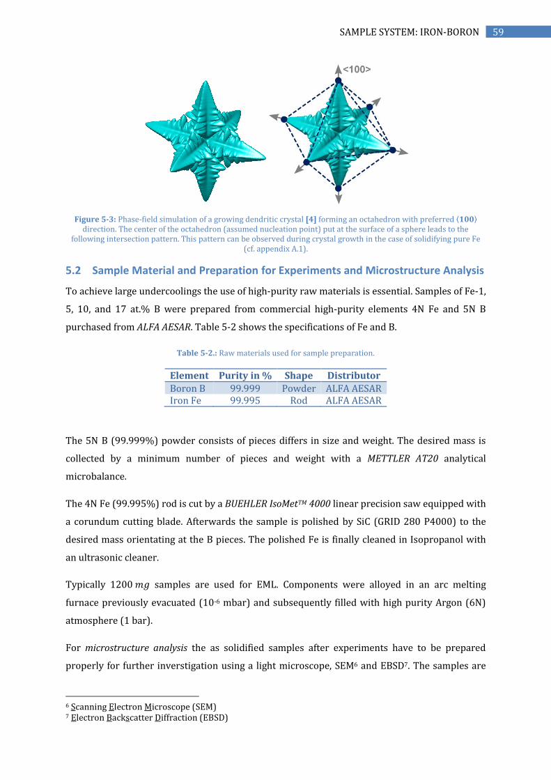
59 SAMPLE SYSTEM: IRON-BORON
Figure 5-3: Phase-field simulation of a growing dendritic crystal [4] forming an octahedron with preferred ⟨𝟏𝟎𝟎⟩ direction. The center of the octahedron (assumed nucleation point) put at the surface of a sphere leads to the
following intersection pattern. This pattern can be observed during crystal growth in the case of solidifying pure Fe (cf. appendix A.1).
5.2 Sample Material and Preparation for Experiments and Microstructure Analysis
To achieve large undercoolings the use of high-purity raw materials is essential. Samples of Fe-1,
5, 10, and 17 at.% B were prepared from commercial high-purity elements 4N Fe and 5N B
purchased from ALFA AESAR. Table 5-2 shows the specifications of Fe and B.
Table 5-2.: Raw materials used for sample preparation.
Element Purity in % Shape Distributor
Boron B 99.999 Powder ALFA AESAR Iron Fe 99.995 Rod ALFA AESAR
The 5N B (99.999%) powder consists of pieces differs in size and weight. The desired mass is
collected by a minimum number of pieces and weight with a METTLER AT20 analytical
microbalance.
The 4N Fe (99.995%) rod is cut by a BUEHLER IsoMetTM 4000 linear precision saw equipped with
a corundum cutting blade. Afterwards the sample is polished by SiC (GRID 280 P4000) to the
desired mass orientating at the B pieces. The polished Fe is finally cleaned in Isopropanol with
an ultrasonic cleaner.
Typically 1200 𝑚𝑔 samples are used for EML. Components were alloyed in an arc melting
furnace previously evacuated (10-6 mbar) and subsequently filled with high purity Argon (6N)
atmosphere (1 bar).
For microstructure analysis the as solidified samples after experiments have to be prepared
properly for further inverstigation using a light microscope, SEM6 and EBSD7. The samples are
6 Scanning Electron Microscope (SEM) 7 Electron Backscatter Diffraction (EBSD)

60 SAMPLE SYSTEM: IRON-BORON
cut by a diamond wire saw and embedded in a conducting amorphous material. The cross-
section surface is polished by using SiC abrasive paper (GRID 280 P4000) followed by alumina
and silica suspension to remove any residual damage due to cutting and grinding.

61 EXPERIMENTAL RESULTS AND DISCUSSION
6 EXPERIMENTAL RESULTS AND DISCUSSION
In this chapter the experimental results are presented and discussed within current
solidification models. The main focus of this thesis lies on the growth kinetics in the Fe-B system
for dendritic growth (Fe-1, 5, 10 at.% B) and eutectic growth (Fe-17 at.% B) by measuring and
modelling the growth velocity 𝑉(∆𝑇, 𝑈0) as a function of undercooling ∆𝑇 influenced by different
fluid flow conditions with varying fluid flow velocity 𝑈0.
During the investigations on the Fe-B binary system, the videos showed unexpected growth
morphologies which changes if concentration, undercooling and fluid flow conditions are
altered. Especially the observation of bent growing dendrites is significant.
The error of the measured undercooling ∆𝑇 is estimated as ±5 𝐾 according to the unknown
emissivity, the measurement accuracy of the infrared pyrometer, and the uncertainty of the
temperature-time profile (caused by sample moving) which was used to determine the liquidus
temperature as well as the maximum undercooling before rapid solidification (see chapter 4.1).
The error of the growth velocity 𝑉 differs from 5% up to 25% depending on the precision of the
measured sample diameter (±0.1 𝑚𝑚), the quality of the video (resolution), and the visibility of
the full solidification process which is sometimes partially hidden because of the sample rotation
during solidification. The videos are analysed to measure the growth velocity according to
appendix A.1. For reasons of clarity no error bars are plotted in the graphs. However the scatter
of data points represents the uncertainty of the measured data. The used models for calculation
to describe the experimental results are in good agreement with experiments and show major
trends which qualitatively reproduce significant effects like solute trapping. Some material and
physical parameters are not well known, like the velocity dependent partition coefficient 𝑘, the
stability constant 𝜎, the anisotropy of the interfacial energy 휀, and the kinetic growth coefficient
𝜇𝐾 , which were chosen as “best fit” parameters to describe the experimental results within the
order of magnitude given by literature.
6.1 Growth Morphology and Microstructure
Figure 6-1 shows an overview of the observed growth morphologies for pure Fe, Fe-1, 5, 10 and
17 at.% B at low and high undercoolings. As described in section A.1 pure Fe solidifies in an
octahedron shape where the intersection of the sample surface results in a rhombohedral
pattern. With increasing B concentration the observed growth fronts change with respect to a
regular shape, in contrast and sharpness.

62 EXPERIMENTAL RESULTS AND DISCUSSION
Figure 6-1: Growth morphologies for pure Fe, Fe-1, 5, 10, and 17 at.% B at low and high undercoolings.

63 EXPERIMENTAL RESULTS AND DISCUSSION
Figure 6-2: Surface of Fe-5 at.% B sample.
The microstructure of selected Fe-1, 5 and 10 at.% samples with different undercoolings were
analysed in order to check for dendritic solidification. All investigated samples show a typical
dendritic structure. Figure 6-2 shows the dendritic microstructure of a Fe-5 at.% B sample
surface and Figure 6-3 the dendritic network of a Fe-10 at.% B sample solidified with an
undercooling ∆𝑇 = 110 𝐾. The crossection of the same Fe-10 at.% B sample implies curved
dendrites which will be discussed in section 6.2.
Figure 6-3: SEM image of a Fe-10at.% B 1g-EML sample surface shows a network of dendritic structure which was solidified at an undercooling of ∆𝑻 = 𝟏𝟎𝟖 𝑲.

64 EXPERIMENTAL RESULTS AND DISCUSSION
Figure 6-4: Cross-section SEM image of a Fe-10 at.% B sample.
Since the high speed video camera recordings show unique and significant solidification
morphologies it should be possible to find matching patterns in the as solidified microstructure
of the sample surface. Figure 6-7 shows an SEM image of a Fe-1 at.% B sample surface and the
corresponding video recording solidification pathway. Similar patterns are visible in both
images however a definite relation could not be found.
Figure 6-5: Sample surface (SEM) in comparison with the growth morphology visible in the high-speed video (snapshot) during solidification process. Similar structures can be observed but not identified/matched exactly.
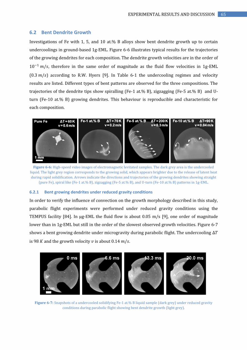
65 EXPERIMENTAL RESULTS AND DISCUSSION
6.2 Bent Dendrite Growth
Investigations of Fe with 1, 5, and 10 at.% B alloys show bent dendrite growth up to certain
undercoolings in ground-based 1g-EML. Figure 6-6 illustrates typical results for the trajectories
of the growing dendrites for each composition. The dendrite growth velocities are in the order of
10−1 𝑚/𝑠, therefore in the same order of magnitude as the fluid flow velocities in 1g-EML
(0.3 𝑚/𝑠) according to R.W. Hyers [9]. In Table 6-1 the undercooling regimes and velocity
results are listed. Different types of bent patterns are observed for the three compositions. The
trajectories of the dendrite tips show spiralling (Fe-1 at.% B), zigzagging (Fe-5 at.% B) and U-
turn (Fe-10 at.% B) growing dendrites. This behaviour is reproducible and characteristic for
each composition.
Figure 6-6: High-speed video images of electromagnetic levitated samples. The dark grey area is the undercooled
liquid. The light grey region corresponds to the growing solid, which appears brighter due to the release of latent heat
during rapid solidification. Arrows indicate the directions and trajectories of the growing dendrites showing straight
(pure Fe), spiral like (Fe-1 at.% B), zigzagging (Fe-5 at.% B), and U-turn (Fe-10 at.% B) patterns in 1g-EML.
6.2.1 Bent growing dendrites under reduced gravity conditions
In order to verify the influence of convection on the growth morphology described in this study,
parabolic flight experiments were performed under reduced gravity conditions using the
TEMPUS facility [84]. In µg-EML the fluid flow is about 0.05 m/s [9], one order of magnitude
lower than in 1g-EML but still in the order of the slowest observed growth velocities. Figure 6-7
shows a bent growing dendrite under microgravity during parabolic flight. The undercooling ∆𝑇
is 98 𝐾 and the growth velocity 𝑣 is about 0.14 𝑚/𝑠.
Figure 6-7: Snapshots of a undercooled solidifying Fe-1 at.% B liquid sample (dark grey) under reduced gravity
conditions during parabolic flight showing bent dendrite growth (light grey).

66 EXPERIMENTAL RESULTS AND DISCUSSION
Table 6-1: Highest undercoolings ∆𝑻 and corresponding dendrite growth velocities 𝒗 for Fe-1, 5 and 10 at.% B where
bent dendrite growth has been observed so far. Data for pure Fe is added for comparison.
Undercooling
T [K]
Dendrite growth
velocity v [m/s] Observed pattern
1g
–E
ML
Pure Fe 60 0.6 Straight, no bending
Fe-1 at.% B 70 0.2 Spiral growth
Fe-5 at.% B 200 0.3 Zigzagging
Fe-10 at.% B 110 0.05 U-turn
TEMPUS
(𝝁𝒈 − 𝑬𝑴𝑳) Fe-1 at.% B 100 0.14 Spiral/Zigzagging
6.2.2 Microstructure of bent dendrites
Figure 6-8 shows the cross section microstructure of a bent dendrite with SEM and EBSD of a Fe-
10 at.% B sample. The sample was processed in 1g-EML and solidified at an undercooling ∆𝑇 of
110 𝐾.
Figure 6-8: SEM and EBSD images of a cross section of Fe-10 at.% B solidified at an undercooling ∆T of 110K in 1g-
EML showing a bent dendrite. The bending occurs mainly in the light blue region and at its transitions to the dark blue
and green region, respectively.
6.2.3 Discussion
The trajectories of the dendrite tips show spiralling, zigzagging, and U-turn patterns for growing
dendrites. So far we did not observe bent growing dendrites in any other metallic materials we
investigated except multicomponent steel alloy. The findings appear to be relevant only for Fe-
based alloys.

67 EXPERIMENTAL RESULTS AND DISCUSSION
Figure 6-9: Schematic view of an electromagnetic levitation facility and levitated liquid sample with stream lines of fluid flow as indicated inside the melt [60]
In general, the dendritic solidification is a competition between heat/solute diffusion and
surface energy [10]. B is poorly soluble in Fe [6]. According to growth models, a solute pile up
exists at the solid-liquid interface of the dendrite tip, which slows down the dendrite growth
velocity. Additionally, fluid flow influences the thermal and solute gradients ahead of the solid-
liquid interface. In particular, the fluid flow velocity inside the melt in 1g-EML is in the same
order of magnitude as the growth velocity itself. Figure 6-9 shows schematically the calculated
fluid flow loops inside a laminar liquid sample according to P. Galenko et al. [60]. There seems to
be a weak correlation between the fluid flow loops inside the liquid sample and the trajectories
of the observed bent growing dendrites. More advanced investigations are needed to confirm
this. Even under reduced gravity conditions with weaker fluid flow velocity the bent dendrite
growth occurs for Fe-1 at.% B.
The microstructure of solidified samples showed that the effect of bent dendrites seems to be
mainly sample-surface dominated. Up to now we were unable to find significant bent dendrites
in the bulk microstructure of the samples. This could be explained due to coarsening and
fragmentation of the as solidified microstructure. The cross section microstructure of solidified
sample (Figure 6-8) indicates a stepwise breaking of the dendrite. Different crystal orientations
of the grains are represented in different colors. A bending occurs mainly in the middle part
(light blue region) and at its transitions to the dark blue and green region.
Regarding bent growing dendrites, one possible explanation was given by A. M. Mullis in 1999
[96] simulated dendritic bending and rosette formation during solidification under forced fluid
flow perpendicular to the growth direction in a shearing flow. So far it is unclear whether the

68 EXPERIMENTAL RESULTS AND DISCUSSION
presented experiments show an actual bent growth or deformation during growth. Phase-field
modelling could reproduce the measured bending/deformation during solidification as reported
by M. Yamaguchi and C. Beckermann [97]. They computed elasto-viscoplastic deformation of
growing solid under a linear shear velocity field using the material point method. According to
them, a phase-field model for simultaneous solid deformation and liquid flow is still not
available.
Overall, the Fe-B system shows a weak anisotropy of the solid-liquid interfacial energy which
may explain the observed bent dendrite growth and why this phenomenon was not reported in
for instance Ni-B with a much higher anisotropy [98]. In addition, the described solidification
interface morphology pattern by LIU et al. [99] in undercooled Co-24 at.% Sn eutectic melt
demonstrated a transition to seaweed growth mode due to its weak interface energy anisotropy.
Another possible explanation for the observed bent dendrite growth is given by L. Gránásy et al.
stating that impurities perturb the crystallization process by deflecting the dendrite tip during
growth [100]. These foreign particles act as orientation pinning centers. In the melt a random
field of impurities may exist leading to zigzagging or spiralling dendrites.
Our study has several limitations for the analysis of the dendrite growth morphologies. First, the
strong oscillation and rotation of the liquid droplet has to be taken into account. In particular,
the shape of the sample changes during crystallization. Second, the nucleation point appears
statistically at a random point on the sample surface, so it is not possible to reproduce the same
experimental conditions. Third, the fluid flow inside the melt is a nonlinear chaotic process and
non-predictable. Fourth, the influence of impurities cannot be neglected.
6.2.4 Conclusion
The research shows bent growing dendrites under different fluid flow conditions. This
phenomenon has been observed in-situ, as far as we know, for the first time in solidifying metals
during levitation. In the case of Fe-10 at.% B in 1g-EML the effect was stronger than for Fe-1 and
5 at% B. Bent dendrite growth could also been observed for Fe-1 at.% B under micro-gravity
conditions during parabolic flight with weaker fluid flow compared to 1g-EML.
The cause of the observed bent dendrite growth is unclear. Impurities cannot be neglected and
should be considered as a possible explanation to the growth behaviour. Unless the fluid flow
and its influence on the thermal and/or concentration gradients at the growing dendrite tip may
cause the growth of bent dendrites. It is well known that a growing dendrite follows the largest
temperature gradient. For instance, future research using an infrared camera could help to
clarify and visualize the thermal field around the growing dendrite.
Finally the effect of bent growing dendrites may be used to manipulate the microstructure
development during solidification. For example, dendrites could be bent during growth to follow

69 EXPERIMENTAL RESULTS AND DISCUSSION
the curving of a turbine blade or guided growing dendrites of semiconductor on substrates could
lead to new technologies.
6.3 Dendrite Growth Velocity 𝑽 versus Undercooling ∆𝑻
The Fe-B dendrite growth velocities 𝑉 are measured as a function of undercooling ∆𝑇.
Experiments were performed in electromagnetic levitator under different fluid flow conditions:
terrestrial 1g-EML and µg-EML TEMPUS facility during parabolic flight. Additional experiments
for Fe-10 at.% B were done in a quartz glass crucible without levitation in a 1g-EML facility.
Furthermore melt fluxing experiments (MF) were performed for Fe-1, 5, and 10 at.% B under
influence of a high magnetic field up to 6 𝑇.
1g-EML:
Pure Fe
Fe-1 at.% B
Fe-5 at.% B
Fe-10 at.% B
Fe-17 at.% B
0 50 100 150 200 250 3001E-3
0,01
0,1
1
10
Gro
wth
velo
city V
[m
/s]
Undercooling T [K]
Figure 6-10: Overview of dendritic Fe, Fe-1, 5, 10 and eutectic 17 at.%B 1g-EML results: Half-logarithmic plot of the growth velocity 𝑽 as a function of undercooling ∆𝑻. The dashed lines are given as a guide for the eye to show main
trends.
Figure 6-10 gives an overview about the measured growth velocities for pure Fe, Fe-1, 5 and 10
at.% (including also the eutectic composition Fe-17 at.% B) which are presented and discussed
in the following. Dashed lines are given as a guide for the eye. The overview shows clearly the
influence of B concentration slowing down the growth velocity. The used sharp interface model
for modelling dendritic growth velocities (pure Fe, Fe-1, 5 and 10 at.%) as a function of
undercooling is described in chapter 2.

70 EXPERIMENTAL RESULTS AND DISCUSSION
6.3.1 Pure Fe
In order to study the effect of alloying B to Fe it is essential to firstly measure pure Fe for
comparison. In addition, these results are compared to Ni and Ni-B alloys. Figure 6-11 shows the
results of the dendritic growth velocity for pure Fe and Ni as a function of undercooling
including the LKT-model predictions. Fe has a monotonous behaviour with increasing
undercooling from some 𝑐𝑚/𝑠 at low undercoolings up to 50 𝑚/𝑠 at about 300 𝐾 undercooling.
The videos show a regular, as expected for cubic metals, growth morphology (see section 6.1)
with a visible growth front at the sample surface which is the intersection of an octahedral
shaped grain. This can be explained by the growth of dendrites along ⟨100⟩ directions. The
tracing of the dendrite tip pathway as the apex of a growing pyramid gives a precise
determination of the propagating tip and its velocity inside the spherical sample (see A.1 Video
Analysis). According to its equilibrium phase diagram Fe solidifies primarily into bcc phase
whereas Ni solidifies into fcc. Furthermore Ni shows a different growth behaviour as Fe at high
undercoolings. In the case of Ni, above ∆𝑇 > 180 𝐾 (𝑉 > 40 𝑚/𝑠) the shape at the sample
surface changes from an octahedral to an isotropic growth front. BASSLER et al. [101] suggest that
the growing dendrites thermally interact with each other. The dendrites become more closely
spaced and the thermal fields surrounding each dendrite begin to overlap. However this
behaviour cannot be observed in Fe but may occur at undercoolings above 300 𝐾.
0 50 100 150 200 250 300
0
10
20
30
40
50
60
70Ni:
Eckler 1994
Model
Fe:
Schleip 1990
Current work
Model
Dendri
te G
row
th V
elo
city V
[m
/s]
Undercooling T [K]
Figure 6-11: Dendrite Growth Velocity 𝑽 of Fe and Ni as a function of undercooling ∆𝑻. The parameter used for modelling are listed in Table 6-2.
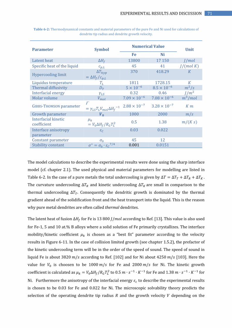
71 EXPERIMENTAL RESULTS AND DISCUSSION
Table 6-2: Thermodynamical constants and material parameters of the pure Fe and Ni used for calculations of
dendrite tip radius and dendrite growth velocity.
Parameter Symbol Numerical Value
Unit Fe Ni
Latent heat ∆𝐻𝑓 13800 17 150 𝐽/𝑚𝑜𝑙
Specific heat of the liquid 𝑐𝑝,𝐿 45 41 𝐽/(𝑚𝑜𝑙 𝐾)
Hypercooling limit ∆𝑇ℎ𝑦𝑝
= ∆𝐻𝑓 𝑐𝑝,𝐿⁄
370 418.29 𝐾
Liquidus temperature 𝑇𝐿 1811 1728.15 𝐾 Thermal diffusivity 𝐷𝑇 5 × 10⁻⁶ 8.5 × 10⁻⁶ 𝑚2/𝑠 Interfacial energy 𝛾𝐿𝑆 0.32 0.46 𝐽/𝑚2 Molar volume 𝑉𝑚𝑜𝑙 7.09 × 10⁻⁶ 7.08 × 10⁻⁶ 𝑚3/𝑚𝑜𝑙
GIBBS-THOMSON parameter
= 𝛾𝐿𝑆𝑇𝐿𝑉𝑚𝑜𝑙∆𝐻𝑓−1
2.88 × 10⁻⁷ 3.28 × 10⁻⁷ 𝐾 𝑚
Growth parameter 𝑽𝟎 1000 2000 𝑚/𝑠 Interfacial kinetic coefficient
𝜇𝑘= 𝑉0∆𝐻𝑓/𝑅𝐺𝑇𝐿
2 0.5 1.38 𝑚/(𝐾 𝑠)
Interface anisotropy parameter
휀𝐶 0.03 0.022
Constant parameter 𝜎0 45 12 Stability constant 𝜎∗ = 𝜎0 ∙ 휀𝐶
7/4 0.001 0.0151
The model calculations to describe the experimental results were done using the sharp interface
model (cf. chapter 2.1). The used physical and material parameters for modelling are listed in
Table 6-2. In the case of a pure metals the total undercooling is given by ∆𝑇 = ∆𝑇𝑇 + ∆𝑇𝑅 + ∆𝑇𝐾 .
The curvature undercooling ∆𝑇𝑅 and kinetic undercooling ∆𝑇𝐾 are small in comparison to the
thermal undercooling ∆𝑇𝑇. Consequently the dendritic growth is dominated by the thermal
gradient ahead of the solidification front and the heat transport into the liquid. This is the reason
why pure metal dendrites are often called thermal dendrites.
The latent heat of fusion ∆𝐻𝑓 for Fe is 13 800 𝐽/𝑚𝑜𝑙 according to Ref. [13]. This value is also used
for Fe-1, 5 and 10 at.% B alloys where a solid solution of Fe primarily crystallizes. The interface
mobility/kinetic coefficient 𝜇𝑘 is chosen as a “best fit” parameter according to the velocity
results in Figure 6-11. In the case of collision limited growth (see chapter 1.5.2), the prefactor of
the kinetic undercooling term will be in the order of the speed of sound. The speed of sound in
liquid Fe is about 3820 𝑚/𝑠 according to Ref. [102] and for Ni about 4250 𝑚/𝑠 [103]. Here the
value for 𝑉0 is choosen to be 1000 𝑚/𝑠 for Fe and 2000 𝑚/𝑠 for Ni. The kinetic growth
coefficient is calculated as 𝜇𝑘 = 𝑉0∆𝐻𝑓/𝑅𝐺𝑇𝐿2 to 0.5 𝑚 ∙ 𝑠−1 ∙ 𝐾−1 for Fe and 1.38 𝑚 ∙ 𝑠−1 ∙ 𝐾−1 for
Ni. Furthermore the anisotropy of the interfacial energy 휀𝑐 to describe the experimental results
is chosen to be 0.03 for Fe and 0.022 for Ni. The microscopic solvability theory predicts the
selection of the operating dendrite tip radius 𝑅 and the growth velocity 𝑉 depending on the

72 EXPERIMENTAL RESULTS AND DISCUSSION
magnitude of the anisotropy of the interfacial energy 휀𝑐 in terms of a dimensionless stability
parameter 𝜎∗ = 𝜎0 ∙ 휀𝑐7/4
. As a best fit parameter 𝜎∗ is determined to be 0.001 for Fe and 0.0151
for Ni. The theoretical operating dendrite tip radius 𝑅 as a function of undercooling is plotted in
Figure 6-12 for Fe and Ni. Obviously a thinner operating dendrite tip radius for Ni is consistent
with the faster growth of Ni compared to Fe. A thin dendrite grows faster as a thick one. Pure Fe
crystallises in body-centered cubic (bcc) crystal structure whereas pure Ni crystallises in face-
centered cubic (fcc) crystal structure. An Fe atom in a bcc crystal has 8 and a Ni atom in a fcc
crystal has 12 nearest neighbours. HOLLAND-MORITZ et al. investigated the short-range order and
coordination number 𝑍 in undercooled Fe and Ni liquids by neutron diffraction experiments
[104]. Atoms joining the solid from the liquid have in the case of Ni (fcc) a higher possibility to
attach which can explain the faster dendritic growth of Ni. The crystallization kinetics in fcc and
bcc metals were investigated with MD simulations by ASHKENAZY and AVERBACK [105]. Their
results show two different temperature regimes. In MD simulations for hard spheres it could be
shown that the reported velocity difference in bcc and fcc crystallization is related to kinetic
factors and not to an anisotropy in the free energy [2, 106].
0 50 100 150 200 250 300
10-7
10-6
10-5
10-4
Theoretical operating dendrite tip radius:
Fe
Ni
Dendrite
Tip
Radiu
s R
[m
]
Undercooling T [K]
Figure 6-12: Half-logarithmic plot of the theoretical operating dendrtite tip Radius 𝑹 as a function of undercooling ∆𝑻 for Ni (dashed blue) and Fe (solid red).
The total undercooling ∆𝑇 for Fe and Ni split into different undercooling contributions which are
shown in Figure 6-13. The thermal undercooling ∆𝑇𝑇 is dominating the growth behaviour
(thermal dendrite) while the kinetic undercooling ∆𝑇𝐾 increases with rising undercooling. The
contribution of the curvature undercooling ∆𝑇𝑅 due to the GIBBS-THOMSON effect is smaller than
5 𝐾 over the entire undercooling range accessible by the experiments and therefore neglectable
small. However the difference between Fe and Ni is significant in the case of the curvature
undercooling ∆𝑇𝑅.

73 EXPERIMENTAL RESULTS AND DISCUSSION
0 50 100 150 200 250 3001E-4
1E-3
0,01
0,1
1
10
100
Ni:
Thermal undercooling TT
Kinetic undercooling TK
Curvature undercooling TR
Fe:
Thermal undercooling TT
Kinetic undercooling TK
Curvature undercooling TR
Ni
TK
TR
Co
ntr
ibu
tio
n o
f u
nd
erc
oo
ling
[K
]
Undercooling T [K]
TT
Fe
Figure 6-13: Contributions of undercooling as a function of the total undercooling ∆𝑻 for Fe (red) and Ni (blue): Thermal undercooling ∆𝑻𝑻 (dashed), kinetic undercooling ∆𝑻𝑲 (solid) and curvature undercooling
∆𝑻𝑹 (dotted).
The theoretical influence of convection on the growth velocity is plotted in a half-logarithmic
plot in Figure 6-14 for different fluid flow velocities 𝑈0 = 0.05 𝑚/𝑠 and 0.3 𝑚/𝑠 which
correspond to the theoretical values in 𝜇g-EML and 1g-EML [9]. In a pure metal the fluid flow
acts on the thermal gradient field ahead of the growing dendrite as described in chapter 2.2.
Consequently with increasing fluid flow the temperature gradient gets steeper and the dendrite
grows faster while the heat transport is enhanced. The thermal undercooling contribution ∆𝑇𝑇 is
plotted in Figure 6-15 as a function of the total undercooling ∆𝑇 and growth velocity 𝑉 for
different fluid flow conditions. In the case of an alloy the influence of convection on the
concentration field ahead of the growing dendrite is much stronger (see 6.3.2, 6.3.3, and 6.3.4).
This is reasonable because the thermal diffusion (10−5 𝑚/𝑠) is much larger than the mass
diffusion (10−9 𝑚/𝑠).
It should be mentioned that fluid-flow also acts on phase selection and nucleation in
undercooled liquid metals as shown by HYERS et al. [107]. However this fact is not included in
the sharp interface model which was used to model the growth velocities as a function of
undercooling.

74 EXPERIMENTAL RESULTS AND DISCUSSION
0 50 100 150 200 250 3000,1
1
10
Fe:
Schleip 1990
Current work
U0 = 0 m/s
U0 = 0.05 m/s (g-EML)
U0 = 0.3 m/s (1g-EML)
U0 = 1 m/s
U0 = 3 m/s
U0 = 10 m/s
Dendrite
Gro
wth
Velo
city V
[m
/s]
Undercooling T [K]
U0
Figure 6-14: Half-logarithmic plot of Fe dendrite growth velocity 𝑽 as a function of undercooling ∆𝑻 for different fluid flow 𝑼𝟎.
0 50 100 150 200 250 3000
50
100
150
200
Co
ntr
ibutio
n o
f th
erm
al u
nd
erc
oo
ling
TT [
K]
Undercooling T [K]
Thermal Undercooling TT:
U0 = 0 m/s
U0 = 0.05 m/s
U0 = 0.3 m/s
U0 = 1 m/s
U0 = 3 m/s
U0 = 10 m/s
U0
0 5 10 15 20 25 30 35 40 45 500
25
50
75
100
125
150
175
200
225
Co
ntr
ibu
tio
n o
f th
erm
al u
nd
erc
oo
ling
T
T [
K]
Dendrite Growth Velocity V [m/s]
Thermal Undercooling TT:
U0 = 0.05 m/s (g-EML)
U0 = 0.03 m/s (1g-EML)
U0 = 1 m/s
U0 = 3 m/s
U0 = 10 m/s
U0
Figure 6-15: Thermal undercooling ∆𝑻𝑻 for Fe plotted as a function of the total undercooling ∆𝑻 and the dendrite growth velocity 𝑽 for different fluid flow 𝑼𝟎.

75 EXPERIMENTAL RESULTS AND DISCUSSION
0 50 100 150 200 250 3000,0
0,1
0,2
0,3
0,4
0,5
0,6
0,7
0,8
0,9
1,0
Fe
Contr
ibution o
f curv
atu
re u
nderc
oolin
g
TR [K
]
Undercooling T [K]
Curvature Undercooling TR:
U0 = 0 m/s
U0 = 0.05 m/s
U0 = 0.3 m/s
U0 = 1 m/s
U0 = 3 m/s
U0 = 10 m/s
U0
Figure 6-16: Contribution of curvature undercooling ∆𝑻𝑹 to the total undercooling ∆𝑻 plotted for diffent fluid flow 𝑼𝟎.
The fluid flow velocity of 𝑈0 = 10 𝑚/𝑠 to describe the 1g-EML experimental results is physical
unrealistic. The used two-dimensional model underestimates the heat and mass transport by
convection. Recently, GAO et al. investigated dendrite growth velocities in an undercooled melt of
pure Ni under static magnetic field (up to 6 𝑇) [108]. The used three-dimensional model by
ALEXANDROV and GALENKO [109] can describe the growth velocity results as a function of
undercooling. This demonstrate a realistic description of dendritic growth kinetics of pure
substances with convection due to stronger heat and mass transport as in two-dimensional
models.

76 EXPERIMENTAL RESULTS AND DISCUSSION
6.3.2 Fe-1 at.% B
Figure 6-17 shows the results of dendrite growth velocity 𝑉 as a function of undercooling ∆𝑇 for
Fe 1g-EML and Fe-1 at.% B 1g-EML and 𝜇g-EML. By alloying 1 at.% B to Fe the growth velocity
for small undercoolings drops down essentially to the range of velocities of 𝑐𝑚/𝑠. For small
undercoolings the dendrite growth velocities of the dilute Fe-B alloy stay much smaller than
those of pure Fe. At an undercooling of about 160 𝐾 the growth velocity of Fe-1 at.% B shows a
sharp increase to about 14 𝑚/𝑠. This effect is called solute trapping which is described in
chapter 1.5.3. Table 6-3 lists the material parameter used for modelling of dendrite growth. A
similar growth behaviour can be observed in the Ni-B system. The transition of diffusion limited
growth of dendrites (solutal growth) to thermally controlled solidification was proven by Eckler
in 1992 [110]. Figure 6-18 shows their results for Ni-B. Solute trapping for Ni-1 at.% B occurs at
a higher undercooling (> 200 𝐾) compared to Fe-1 at.% B. In the case of dilute Fe-1 at.% B the
plot can be divided into 3 regimes:
Solutal growth (80 𝐾 < ∆𝑇 < 160 𝐾),
Solutal and thermal growth (plateau ∆𝑇 > 160 𝐾),
Thermal growth, almost partition less solidification (∆𝑇 > 280 𝐾).
The first regime is the diffusion limited (80 𝐾 < ∆𝑇 < 160 𝐾) which is described well by the
model. Second regime is the transition from diffusion limited to thermally controlled
(160 𝐾 < ∆𝑇 < 190 𝐾) with the active development of solute trapping. Third regime is the
totally thermal controlled part with a high scattering in data.
0 50 100 150 200 250 300
0
10
20
30
40
50
Fe:
1g-EML
Fe-1 at.% B:
1g-EML
g-EML
Model U0 = 0 m/s
De
ndrite
Gro
wth
Ve
locity V
[m
/s]
Undercooling T [K]
Figure 6-17: Dendrite growth velocity as a function of undercooling for Fe and Fe-1 at.% B.

77 EXPERIMENTAL RESULTS AND DISCUSSION
Table 6-3: Thermodynamical constants and material parameters of the Fe-1 at.% B composition used for calculations
of dendrite tip radius and dendrite growth velocity.
Parameter Symbol Numerical value Unit
Concentration of Boron 𝐶0 10 𝑎𝑡.% Liquidus temperature 𝑇𝑚 1793 𝐾 Latent heat ∆𝐻𝑓 13800 𝐽/𝑚𝑜𝑙
Specific heat of the liquid 𝑐𝑝,𝐿 45 𝐽/(𝑚𝑜𝑙 𝐾)
Hypercooling limit ∆𝑇ℎ𝑦𝑝 = ∆𝐻𝑓 𝑐𝑝,𝐿⁄ 306.7 𝐾
Liquidus slope 𝑚𝑒 −17.14 𝐾/𝑎𝑡.% Partition coefficient 𝑘𝑒 0.001 Diffusion coefficient 𝐷𝐶 5 × 10⁻⁹ 𝑚2/𝑠 Thermal diffusivity 𝐷𝑇 5 × 10⁻⁶ 𝑚2/𝑠 Interfacial energy 𝛾𝐿𝑆 0.31 𝐽/𝑚2 Molar volume 𝑉𝑚𝑜𝑙 7.09 × 10⁻⁶ 𝑚3/𝑚𝑜𝑙 GIBBS-THOMSON coefficient = 𝛾𝐿𝑆𝑇𝐿𝑉𝑚𝑜𝑙∆𝐻𝑓
−1 2.85 × 10⁻⁷ 𝐾 𝑚
Diffusion speed in bulk liquid 𝑉𝐷 14 𝑚/𝑠 Interface diffusion speed 𝑉𝐷𝐼 2.5 𝑚/𝑠 Interfacial kinetic coefficient 𝜇𝑘 = 𝑉0∆𝐻𝑓/𝑅𝐺𝑇𝐿
2 0.118 𝑚/(𝐾 𝑠)
Interface anisotropy parameter 휀𝐶 0.03 Stability constant parameter 𝜎0 45 Stability constant 𝜎∗ = 𝜎0 ∙ 휀𝐶
7/4 0.097 First asymptotic parameter 𝑎1 0.3 Second asymptotic parameter 𝑎2 0.02
Figure 6-18: Results by Eckler et al. taken from Ref. [110]. Dendrite growth velocities 𝑽 for Ni, Ni-0.7, and Ni-1 at.% B as a function of undercooling ∆𝑻 (left graph). The growth velocities show a sharply rise at a critical undercooling ∆𝑻∗ = 𝟐𝟏𝟒 𝑲 for Ni-0.7 at.% B and ∆𝑻∗ = 𝟐𝟔𝟕 𝑲 for Ni-1 at.% B. This effect of solute trapping can be seen in the
concentration (upper right graph) and dendrite tip radius (lower right graph).

78 EXPERIMENTAL RESULTS AND DISCUSSION
The diffusion velocity 𝑉𝐷 of B in liquid Fe can be estimated to be around 14 𝑚/𝑠 by the
experimental data where solute trapping occurs, wheras the diffusion velocity at the interface
𝑉𝐷𝐼 is about 2.5 𝑚/𝑠. The velocity dependence of the partition coefficient 𝑘(𝑉) is plotted in
Figure 6-19. For 𝑉 = 0 𝑚/𝑠 the partition coefficient has the value of the equilibrium partition
coefficient 𝑘𝐸 = 0.001. With rising solidification velocity 𝑘 increases until reaching the diffusion
velocity 𝑉𝐷where solute trapping occurs and 𝑘 remains 1 for 𝑉 ≥ 𝑉𝐷. This is consistent with the
jump of one magnitude in growth velocity from 𝑐𝑚/𝑠 to the diffusion velocity of 𝑚/𝑠 at an
undercooling ∆𝑇 ≈ 160 𝐾.
0 50 100 150 200 250 300 350
0,0
0,2
0,4
0,6
0,8
1,0
Velo
city d
ep
end
ent
pa
rtitio
n c
oeff
icie
nt k(V
)
Undercooling T [K]
Fe-1 at.% B:
k(V)
Figure 6-19: Velocity dependence of the partitioning coefficient 𝒌(𝑽) plotted as a function of undercooling (orange dashed) and growth velocity (red solid). Starting at ∆𝑻 = 𝟎 𝑲 corresponding to a growth velocity 𝑽 = 𝟎 𝒎/𝒔 with the value of the equilibrium partition coefficient 𝒌𝑬 = 𝟎.𝟎𝟎𝟏 and rising until reaching the diffusion velocity 𝑽𝑫 = 𝟏𝟒 𝒎/𝒔
at an undercooling ∆𝑻 = 𝟏𝟔𝟎 𝑲 where solute trapping occurs and 𝒌 becomes 𝟏 for 𝑽 ≥ 𝑽𝑫.
The crystal growth velocity is the decisive parameter governing the trapping of solute in the
solvent material. The concentrations at the dendrite tip in the liquid phase 𝑐𝐿∗ and in the solid
phase 𝑐𝑆∗ is given by:
𝑐𝐿∗ =
𝑐01 − [1 − 𝑘(𝑉)] 𝐼𝑣(𝑃𝐶)
,
𝑐𝑆∗ = 𝑘(𝑉)𝑐𝐿
∗ .
Figure 6-20 shows the calculated distribution of 𝑐𝐿∗ and 𝑐𝑆
∗ as a function of undercooling. For
small undercoolings the B concentration 𝑐𝐿∗ grows rapidly with rising undercooling due to solute
rejection into the liquid. This leads to a pile up of B concentration ahead of the growing dendrite
tip. The growing crystal solves B according to its equilibrium partition coefficient 𝑘𝐸 which
limits the growth velocity due to the finite diffusion velocity of B atoms in the liquid Fe. This
process dominates and slows down the growth velocity 𝑉 to some 𝑐𝑚/𝑠 until solute trapping
increases the solute concentration 𝑐𝑆∗ in the crystal. The sharp increase of the dendrite growth
velocity at an undercooling of about 160 𝐾 implies solute trapping. As a consequence, the
concentration 𝑐𝐿∗ in the liquid phase approaches the nominal concentration of the composition (1
at. % B) while the concentration 𝑐𝑆∗ of the crystal increases to the nominal composition.
0 5 10 15 20 25 30
0.0
0.2
0.4
0.6
0.8
1.0
V m s
kV

79 EXPERIMENTAL RESULTS AND DISCUSSION
Obviously, B is trapped beyond its equilibrium partition coefficient leading to a supersaturated
solid solution. At very large undercoolings solidification takes place partitionless.
0 50 100 150 200 250 3000,00
0,25
0,50
0,75
1,00
1,25
1,50
1,75
Co
nce
ntr
atio
n [
at.
% B
]
Undercooling T [K]
Fe-1 at.% B:
cL*
cS*
c0
Figure 6-20: Calculated concentrations 𝒄𝑳∗ and 𝒄𝑺
∗ at the dendrite tip as a function of undercooling.
The total undercooling ∆𝑇 splits into different undercooling terms. The constitutional
undercooling ∆𝑇𝐶 and the curvature undercooling ∆𝑇𝑅 dominate the first regime (∆𝑇 < 160 𝐾)
while the thermal undercooling ∆𝑇𝑇 and the kinetic undercooling ∆𝑇𝐾 dominate the regime for
large undercoolings. The critical undercooling ∆𝑇∗ = 160 𝐾 is also pronounced in the dendrite
tip radius which is plotted in Figure 6-22.
0 50 100 150 200 250 300 3500
50
100
150
200
250
TK
TT
TC
TR
Contr
ibutio
n o
f un
derc
oolin
g [K
]
Undercooling T [K]
Fe-1 at.% B:
Figure 6-21: Contributions of undercooling as a function of the total undercooling ∆𝑻 for Fe-1 at.% B: Constitutional undercooling ∆𝑻𝑪 (blue solid), thermal undercooling ∆𝑻𝑻 (red solid), kinetic undercooling ∆𝑻𝑲 (orange dashed) and
curvature undercooling ∆𝑻𝑹 (green dotted).

80 EXPERIMENTAL RESULTS AND DISCUSSION
0 50 100 150 200 250 300
10-8
10-7
10-6
10-5
Fe-1 at.% B
Pure Fe
Dendrite
Tip
Radiu
s R
[m
]
Undercooling T [K]
Figure 6-22: Dendrite Tip Radius R a s a function of undercooling ∆𝑻.
The growth velocity at about 160 𝐾 where the solute trapping phenomenon occurs another
interesting effect becomes apparent. A very slim growing concentrational dendrite of about
10−8𝑚 radius can grow faster as a thermal dendrite of about 10−6 𝑚. The dendrite growth
velocity of Fe-1 at.% B seems to be even faster than that of pure Fe. This effect has been
observed by ECKLER et al. for Ni-C [111]. They reported anomalously high velocities in the Ni-0.6
at.% C alloy which showed enhanced dendrite growth velocities in comparison with nominal
pure Ni.
At very large undercooling the growth velocity values of Fe-1 at.% cannot be described by the
model. Above an undercooling of 300 𝐾 the velocity rises drastically. This effect and the scatter
of data points could be explained by a shift of primary bcc to primary fcc phase. This is the same
idea as the assumption to explain the difference between Fe and Ni which was already discussed
in section 6.3.1. HOLLAND-MORITZ et al. investigated the short-range order in undercooled Fe and
Ni liquids by neutron diffraction experiments [104]. In brief, for bcc the coordination number is
8 in contrast to 12 in the case of fcc crystal structure. Therefore the attachment kinetics is faster
for 12 instead of 8 nearest neighbours.
The small value of the anisotropy strength parameter 휀𝐶 = 0.03 is an indication to explain bent
dendrite growth which is described in section 6.2. The growing dendrite tip is “sensible” against
concentrational and thermal fluctuations induced by fluid flow. Not only the growth direction is
affected by fluid flow but also the dendrite growth velocity. Therefore the growth velocities are
measured under different fluid flow conditions (µg-EML and melt fluxing with a static magnetic
field). Figure 6-23 shows the dendrite growth velocity as a function of undercooling for 1g-EML

81 EXPERIMENTAL RESULTS AND DISCUSSION
and 𝜇g-EML. In the case of 𝜇g-EML the growth velocities at low undercoolings are as expected
smaller than in 1g-EML. In general the growth velocity is increased by fluid flow. Consequently,
smaller fluid flow velocities lead to slower growth velocities. This influence is strongest for small
undercoolings compared with large undercoolings.
0 50 100 150 200 250 300
0,01
0,1
1
10
Fe-1 at.% B:
1g-EML
g-EML
U0 = 0 m/s
U0 = 0.05 m/s (g-EML)
U0 = 0.3 m/s (1g-EML)
Dend
rite
Gro
wth
Ve
locity V
[m
/s]
Undercooling T [K]
Figure 6-23: Half-logarithmic plot of the dendrite growth velocities as a function of undercooling for Fe-1 at.% B in 1g-EML and 𝝁g-EML. The influence of convection is strongest at low undercooling where the fluid flow velocity inside
the melt is in the same order of magnitude as the growth velocity itself.
6.3.2.1 Microstructure Analysis of Fe-1 at.% B samples
Microstructure of samples processed during parabolic flight are analysed by means of SEM. One
sample is investigated with respect to its microstructure which solidified at slow undercooling
∆𝑇 = 70 𝐾 under microgravity conditions and another sample which solidified at large
undercooling ∆𝑇 = 270 𝐾 (with solute trapping). Samples processed in 𝜇𝑔-EML show typically a
more detailed undisturbed microstructure due to less fluid flow conditions during solidification.
To give a confirmation of solute trapping the interdendritic fraction is estimated and analysed.
Therefore a sample solidified with and without solute trapping is investigated. A homogeneous
distribution of primarily Fe solidifies dendritic. The remaining liquid in the space between
network of dendrite branches after primary solidification leads to coarsening of the actual
dendrites unless the remaining liquid solidifies eutectic. For high undercoolings, where solute
trapping occurs the fraction of interdendritic B content should be less compared to low

82 EXPERIMENTAL RESULTS AND DISCUSSION
undercoolings with no solute trapping. The reason is that B is “trapped” already in the dendritic
structure which means less B remains for the interdendritic eutectic solidification.
Figure 6-24: Interdendritic fraction of parabolic flight samples… Low undercooling (∆𝑻 = 𝟕𝟎 𝑲 ) and high
undercooling (∆𝑻 = 𝟐𝟕𝟎 𝑲) where solute trapping occurs.

83 EXPERIMENTAL RESULTS AND DISCUSSION
6.3.3 Fe-5 at.% B
Fe-5 at.% B shows in the case of 1g-EML experiments a very strong bent growing dendrite
behaviour (zigzagging) as mentioned in section 6.1. Therefore the measured growth velocities
have a large error/scatter and should be interpreted with care. Figure 6-25 shows the
experimental results (1g-EML, 𝜇g-EML and MF) for dendrite growth velocities as a function of
undercooling. Table 6-4 lists the material parameter used for modelling of dendrite growth
velocities. The model describes the data in good agreement also concerning different fluid flow
velocities 𝑈0. The used parameters for modelling Fe-5 at.B growth velocities include the desired
values for the solid-liquid interface free energy 𝛾 = 0.31 𝐽𝑚−2, its anisotropy 휀 = 0.01 which is
weaker than the found value for Fe-1 at.% B, and the kinetic growth coefficient 𝜇𝑘 =
0.04 𝑚𝐾−1𝑠−1 which is also smaller compared to Fe-1 at.% B. However, the appearance of solute
trapping cannot be proofed in the case of Fe-5 at.% B as well as the competition between
primary bcc and fcc structure crystallization. The contributions of undercooling are shown in
Figure 6-26. The solute concentration at the dendrite tip is plotted in Figure 6-28. Figure 6-27
shows a half-logarithmic plot of the theoretical operating dendrite tip radius 𝑅 as a function of
undercooling.
0 50 100 150 200 250 300
0,01
0,1
1
Fe-5 at.% B:
MF (0 Tesla)
MF (1 Tesla)
1g-EML
U0 = 0 m/s
U0 = 0.3 m/s (1g-EML)
U0 = 0.05 m/s (g-EML)
De
nd
rite
Gro
wth
Ve
locity V
[m
/s]
Undercooling T [K]
U0
Figure 6-25: Dendrite growth velocity 𝑽 as a function of undercooling ∆𝑻 for Fe-5 at.% B.

84 EXPERIMENTAL RESULTS AND DISCUSSION
Table 6-4: Thermodynamical constants and material parameters of the Fe-5 at.% B composition used for calculations
of dendrite tip radius 𝑹, dendrite growth velocity 𝑽, undercooling contributions.
Parameter Symbol Numerical value Unit Ref.
Concentration of Boron 𝐶0 5 𝑎𝑡.% Liquidus temperature 𝑇𝑚 1723 𝐾 Latent heat ∆𝐻𝑓 13800 𝐽/𝑚𝑜𝑙
Specific heat of the liquid 𝑐𝑝,𝐿 45 𝐽/(𝑚𝑜𝑙 𝐾)
Hypercooling limit ∆𝑇ℎ𝑦𝑝 = ∆𝐻𝑓 𝑐𝑝,𝐿⁄ 306.7 𝐾
Liquidus slope 𝑚𝑒 −16.56 𝐾/𝑎𝑡.% Partition coefficient 𝑘𝑒 0.001 Diffusion coefficient 𝐷𝐶 1 × 10⁻⁹ 𝑚2/𝑠 Thermal diffusivity 𝐷𝑇 4.5 × 10⁻⁶ 𝑚2/𝑠 Interfacial energy 𝛾𝐿𝑆 0.31 𝐽/𝑚2 Molar volume 𝑉𝑚𝑜𝑙 7.09 × 10⁻⁶ 𝑚3/𝑚𝑜𝑙 GIBBS-THOMSON coefficient = 𝛾𝐿𝑆𝑇𝐿𝑉𝑚𝑜𝑙∆𝐻𝑓
−1 2.7 × 10⁻⁷ 𝐾 𝑚
Growth parameter 𝑉0 - 𝑚/𝑠 Diffusion speed in bulk liquid 𝑉𝐷 14 𝑚/𝑠 Interface diffusion speed 𝑉𝐷𝐼 2.5 𝑚/𝑠 Interfacial kinetic coefficient 𝜇𝑘 = 𝑉0∆𝐻𝑓/𝑅𝐺𝑇𝐿
2 0.04 𝑚/(𝐾 𝑠)
Interface anisotropy parameter 휀𝐶 0.01 Stability constant parameter 𝜎0 5 Stability constant 𝜎∗ = 𝜎0 ∙ 휀𝐶
7/4 0.0086 First asymptotic parameter 𝑎1 0.3 Second asymptotic parameter 𝑎2 0.01
0 50 100 150 200 250 3001E-5
1E-4
1E-3
0,01
0,1
1
10
100
Co
ntr
ibu
tio
n o
f u
nd
erc
oo
ling
[K
]
Undercooling T [K]
TK
TC
TT
TR
Figure 6-26: Contributions of undercooling as a function of the total undercooling ∆𝑻 for Fe-5 at.% B: Constitutional undercooling ∆𝑻𝑪, kinetic undercooling ∆𝑻𝑲 (blue dashed), thermal undercooling ∆𝑻𝑻 (blue dash-dotted), and
curvature undercooling ∆𝑻𝑹 (red dotted)

85 EXPERIMENTAL RESULTS AND DISCUSSION
0 50 100 150 200 250 300
10-8
10-7
10-6
10-5
Dend
rite
Tip
Rad
ius R
[m
]
Undercooling T [K]
Fe-5 at. % B
Figure 6-27: Half-logarithmic plot of the theoretical operating dendrtite tip Radius 𝑹 as a function of undercooling ∆𝑻 for Fe-5 at.% B.
0 50 100 150 200 250 3000
1
2
3
4
5
6
7
8
9
10
11
c0
Co
nce
ntr
atio
n [
at.
% B
]
Undercooling T [K]
Fe-5 at.% B:
cS*
cL*
Figure 6-28: Concentration of B at the grwoing dendrite tip in the liquid 𝒄𝑳∗ (blue) and the solid 𝒄𝑺
∗ (red).

86 EXPERIMENTAL RESULTS AND DISCUSSION
6.3.4 Fe-10 at.% B
Fe-10 at.% B experiments were performed in 1g-EML, µg-EML TEMPUS parabolic flight, and
melt fluxing experiments in a static magnetic field (1 and 2 𝑇).
50 100 150 200 250 300
0,0
0,1
0,2
0,3
0,4
0,5
0,6
Fe-10 at.% B:
Quartz glass crucible
1g-EML
g-EML
MF (0 Tesla)
MF (1 Tesla)
MF (2 Tesla)
U0 = 0 m/s
U0 = 0.05 m/s (g-EML)
U0 = 0.3 m/s (1g-EML)
U0 = 1 m/s
De
nd
rite
Gro
wth
Ve
locity V
[m
/s]
Undercooling T [K]
Figure 6-29: Dendrite growth velocity 𝑽 as a function of undercooling ∆𝑻 for Fe-10 at.% B.
The measured growth velocities for Fe-10 at.% B have a large error/scatter and should be
interpreted with care. This can be explained by influence of fluid flow in 1g-EML, rotation and
oscillation of the samples. The growth velocities might overestimated because of the curved
growth (U-Turn). Figure 6-29 shows the experimental results (1g-EML, 𝜇g-EML and MF) for
dendrite growth velocities as a function of undercooling. Table 6-5 lists the material parameter
used for modelling of dendrite growth velocities. The model describes the experimental data
qualitatively with different fluid flow velocities 𝑈0. The used parameters for modelling Fe-10

87 EXPERIMENTAL RESULTS AND DISCUSSION
at.B growth velocities include the desired values for the solid-liquid interface free energy
𝛾 = 0.31 𝐽𝑚−2, its anisotropy 휀 = 0.01 which is the same for Fe-5 at.% B, and the kinetic growth
coefficient 𝜇𝑘 = 0.006 𝑚𝐾−1𝑠−1 which is smaller compared to Fe-1 and 5 at.% B. The
contributions of undercooling are shown in Figure 6-30. The solute concentration at the
dendrite tip is plotted in Figure 6-31. Figure 6-32 shows a half-logarithmic plot of the theoretical
operating dendrite tip radius 𝑅 as a function of undercooling.
The results for MF with 2 Tesla are as expected similar to 𝜇g-EML. The influence of convection is
strongest for 1g-EML compared to MF and µg.
Table 6-5: Thermodynamical constants and material parameters of the Fe-10 at.% B composition used for
calculations of dendrite tip radius 𝑹, dendrite growth velocity 𝑽, undercooling contributions.
Parameter Symbol Numerical value Unit Ref.
Concentration of Boron 𝐶0 10 𝑎𝑡.% Liquidus temperature 𝑇𝑚 1590 𝐾 Latent heat ∆𝐻𝑓 13800 𝐽/𝑚𝑜𝑙
Specific heat of the liquid 𝑐𝑝,𝐿 45 𝐽/(𝑚𝑜𝑙 𝐾)
Hypercooling limit ∆𝑇ℎ𝑦𝑝 = ∆𝐻𝑓 𝑐𝑝,𝐿⁄ 306.7 𝐾
Liquidus slope 𝑚𝑒 −15.22 𝐾/𝑎𝑡.% Partition coefficient 𝑘𝑒 0.001 Diffusion coefficient 𝐷𝐶 1.2 × 10⁻⁹ 𝑚2/𝑠 Thermal diffusivity 𝐷𝑇 5 × 10⁻⁶ 𝑚2/𝑠 Interfacial energy 𝛾𝐿𝑆 0.31 𝐽/𝑚2 Molar volume 𝑉𝑚𝑜𝑙 7.09 × 10⁻⁶ 𝑚3/𝑚𝑜𝑙 GIBBS-THOMSON coefficient = 𝛾𝐿𝑆𝑇𝐿𝑉𝑚𝑜𝑙∆𝐻𝑓
−1 2.532 × 10⁻⁷ 𝐾 𝑚
Growth parameter 𝑉0 - 𝑚/𝑠 Diffusion speed in bulk liquid 𝑉𝐷 14 𝑚/𝑠 Interface diffusion speed 𝑉𝐷𝐼 2.5 𝑚/𝑠 Interfacial kinetic coefficient 𝜇𝑘 = 𝑉0∆𝐻𝑓/𝑅𝐺𝑇𝐿
2 0.006 𝑚/(𝐾 𝑠)
Interface anisotropy parameter 휀𝐶 0.01 Stability constant parameter 𝜎0 5 Stability constant 𝜎∗ = 𝜎0 ∙ 휀𝐶
7/4 0.00158 First asymptotic parameter 𝑎1 0.1 Second asymptotic parameter 𝑎2 0.029

88 EXPERIMENTAL RESULTS AND DISCUSSION
0 50 100 150 200 250 3001E-3
0,01
0,1
1
10
100Fe-10 at.% B:
Co
ntr
ibu
tio
n o
f u
nd
erc
oo
ling
[K
]
Undercooling T [K]
TC
TK
TR
TT
Figure 6-30: Contributions of undercooling as a function of the total undercooling ∆𝑻 for Fe-10 at.% B: Constitutional undercooling ∆𝑻𝑪, kinetic undercooling ∆𝑻𝑲 (blue dashed), thermal undercooling ∆𝑻𝑻 (blue dash-dotted), and
curvature undercooling ∆𝑻𝑹 (red dotted)
0 50 100 150 200 250 300
0
10
20
30
40
Co
nce
ntr
atio
n [
at.
% B
]
Undercooling T [K]
Fe-10 at.% B:
c0
cL*
cS*
Figure 6-31: Concentration of B at the grwoing dendrite tip in the liquid 𝒄𝑳∗ (blue) and the solid 𝒄𝑺
∗ (red).
0 50 100 150 200 250 30010
-7
10-6
10-5
De
nd
rite
Tip
Ra
diu
s R
[m
]
Undercooling T [K]
Fe-10 at. % B
Figure 6-32: Half-logarithmic plot of the theoretical operating dendrtite tip Radius 𝑹 as a function of undercooling ∆𝑻 for Fe-10 at.% B.

89 EXPERIMENTAL RESULTS AND DISCUSSION
6.4 Eutectic composition Fe-17 at.% B
In this work, rapid solidification of undercooled Fe-17 at.% B eutectic alloy was studied. The
presented eutectic dendrite growth model (Chapter 3: Eutectic growth) is an extension of
previous models [72, 73] for concentrated alloys with non-linear phase-diagram (NLPD). The
measured growth velocity as a function of undercooling is accurately predicted by the current
eutectic dendrite model for concentrated alloys with NLPD. Previous models for dilute alloys
with linear phase-diagram could not predict the measured behavior. To the best knowledge of
the author, this is the first report where experimental results of eutectic dendrite growth
velocities in undercooled melts can be predicted successfully. The experimental and modelling
results were puplished in Scripta Materialia [63].
Eutectic solidification is a cooperative growth of two phases. However the Fe2B phase
additionally competes with the metastable Fe3B phase [112, 113]. The maximum achieved
undercolling was ∆𝑇 = 217 𝐾. Note that, the maximal undercooling in the current work is much
smaller than ∆𝑇 = 386 𝐾 where a metastable Fe3B phase was found [114]. Therefore the studied
eutectic dendrite is assumed to be solely crystallized by a cooperative growth of 𝛾-Fe and Fe2B.
In order to investigate the microstructure of a Fe-17 at.% B sample, an 𝜇𝑔-EML parabolic flight
sample is analysed by SEM.
6.4.1 Eutectic Dendrite Growth Velocities 𝒗(∆𝑻)
The eutectic composition shows a smooth growth front (see section 6.1) which can be estimated
as a spherical morphology. Therefore all videos are analyses as described in chapter A.1 with the
assumption of isotropic growth.
In 1997 BATTEZZATI et al. calculated the dendrite growth velocities for different undercoolings of
Fe-17 at.% B which are tabulated in Table 6-6 [115]. The measured growth veolicities in this
thesis are about one order of magnitude larger than predicted by BATTEZZATI.
Table 6-6: Calculated growth velocities from Battezzati et al. [115] as a first estimation to describe growth behaviour of Fe-17 at.% B
Undercooling ∆𝑻 [𝑲] Calculated growth velocity 𝒗 [𝒎/𝒔]
𝟓𝟎 1.5 × 10⁻⁴ 𝟏𝟎𝟎 5 × 10⁻⁴ 𝟐𝟎𝟎 1.1 × 10⁻³
Therefore a more advanced theoretical approach is needed to describe the growth behaviour of
Fe-17 at.% B eutectic alloy as a function of undercooling. In fact it is not one single primary
phase growing but two phases grow cooperative.

90 EXPERIMENTAL RESULTS AND DISCUSSION
Figure 6-33: Equilibrium phase diagram of the Fe-B eutectic alloy and its metastable extension according to the thermodynamic optimization of Rompaey et al. [116]. It is approximated as the second type of LPD in the TMK model
[68] LPD1, and LPD2 (slopes of equilibrium liquidus are given by the values at the eutectic point).
The equilibrium Fe-B eutectic phase-diagram is shown in Figure 6-33. Its metastable extensions
are calculated according to the thermodynamic treatment of ROMPAEY et al. [116] which is
indicated by solid and dashed lines. The 𝛾-Fe solid-solution phase on the left hand side has a
negligible solubility of B, whereas the Fe2B phase on the right hand side is the stoichiometric
compound with a molar fraction 𝐶𝐹𝑒2𝐵 = 1/3. At the equilibrium eutectic temperature
𝑇𝐸𝑒 = 1454.4 𝐾, the equilibrium partition coefficients are 𝑘𝛾
𝑒 = 0.00115 and 𝑘𝐹𝑒2𝐵𝑒 =
(𝐶𝐹𝑒2𝐵 − 𝑎) (𝐶𝐿∗ − 𝑎) = 0⁄ , respectively. Here 𝑎 = 1/3 is the composition at which the solidus
and liquidus line of Fe2B intersect [117], and 𝐶𝐿∗ is the liquid composition at the interface. Since
𝑘𝛾𝑒 and 𝑘𝐹𝑒2𝐵
𝑒 are negligibly small, the Fe-B eutectic alloy might be approximated reasonably as
the second type of LPD in the TMK model [68]. For 𝑘𝛾𝑒 = 𝑘𝐹𝑒2𝐵
𝑒 = 𝑘𝑒 = 0.001, the absolute
values of the slopes of 𝛾-Fe and Fe2B equilibrium liquidus are 𝑚𝐿𝛾𝑒 = 2030 𝐾 𝑎𝑡.−1 and
𝑚𝐿𝐹𝑒2𝐵𝑒 = 1395 𝐾 𝑎𝑡.−1 respectively indicated by dotted lines in Figure 6-33 as LPD1. In this
case, the eutectic dendrite growth model of Li and Zhou (LZ) [75] is applicable for TMK-kind
LPDs .
The experimental and computed results are summarized in Figure 6-34. In the case of the LZ
model LPD1 the experimental results cannot be predicted which is similar to previous works for
eutectics [73, 74, 118]. Therefore an eutectic dendrite growth model for undercooled
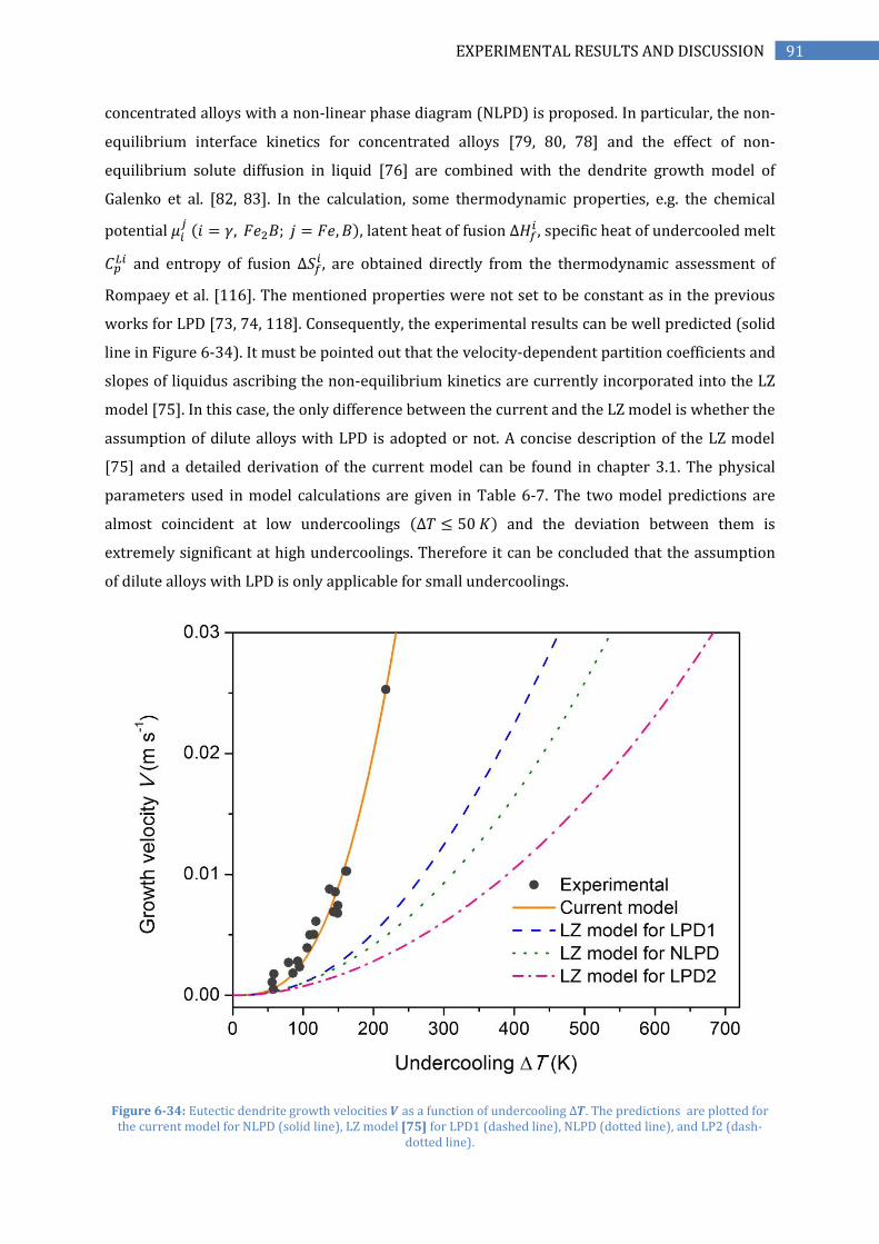
91 EXPERIMENTAL RESULTS AND DISCUSSION
concentrated alloys with a non-linear phase diagram (NLPD) is proposed. In particular, the non-
equilibrium interface kinetics for concentrated alloys [79, 80, 78] and the effect of non-
equilibrium solute diffusion in liquid [76] are combined with the dendrite growth model of
Galenko et al. [82, 83]. In the calculation, some thermodynamic properties, e.g. the chemical
potential 𝜇𝑖𝑗 (𝑖 = 𝛾, 𝐹𝑒2𝐵; 𝑗 = 𝐹𝑒, 𝐵), latent heat of fusion ∆𝐻𝑓
𝑖 , specific heat of undercooled melt
𝐶𝑝𝐿𝑖 and entropy of fusion ∆𝑆𝑓
𝑖 , are obtained directly from the thermodynamic assessment of
Rompaey et al. [116]. The mentioned properties were not set to be constant as in the previous
works for LPD [73, 74, 118]. Consequently, the experimental results can be well predicted (solid
line in Figure 6-34). It must be pointed out that the velocity-dependent partition coefficients and
slopes of liquidus ascribing the non-equilibrium kinetics are currently incorporated into the LZ
model [75]. In this case, the only difference between the current and the LZ model is whether the
assumption of dilute alloys with LPD is adopted or not. A concise description of the LZ model
[75] and a detailed derivation of the current model can be found in chapter 3.1. The physical
parameters used in model calculations are given in Table 6-7. The two model predictions are
almost coincident at low undercoolings (∆𝑇 ≤ 50 𝐾) and the deviation between them is
extremely significant at high undercoolings. Therefore it can be concluded that the assumption
of dilute alloys with LPD is only applicable for small undercoolings.
Figure 6-34: Eutectic dendrite growth velocities 𝑽 as a function of undercooling ∆𝑻. The predictions are plotted for the current model for NLPD (solid line), LZ model [75] for LPD1 (dashed line), NLPD (dotted line), and LP2 (dash-
dotted line).

92 EXPERIMENTAL RESULTS AND DISCUSSION
Table 6-7: Thermodynamical, physical and material parameters of the Fe-17 at.% B eutectic alloy used for modelling.
Parameter Symbol Numerical
value Unit Ref.
Concentration of Boron 𝐶0 17 𝑎𝑡.% Eutectic equilibrium temperature 𝑇𝑒 1454.4 𝐾 Interfacial solute diffusion velocity 𝑉𝐷𝐿
𝐼 0.5 𝑚/𝑠 Solute diffusion velocity in liquid 𝑉𝐷𝐿 1 𝑚/𝑠 Upper limit velocity for interface migration 𝑉0 450 𝑚/𝑠 Solute diffusion coefficient in liquid 𝐷𝐿 3 × 10⁻¹⁰ 𝑚2/𝑠 Thermal diffusion coefficient 𝛼𝐿 1.5 × 10⁻⁵ 𝑚2/𝑠 Molar volume 𝑉𝑚 6.675 × 10⁻⁶ 𝑚3/𝑚𝑜𝑙 Interface tension of 𝜸/𝑳 interface 𝜎𝛾/𝐿 0.3 𝐽/𝑚2
Interface tension of Fe2B interface 𝜎𝐹𝑒2𝐵/𝐿 0.5 𝐽/𝑚2
Anisotropy coefficient 휀𝐶 0.006 Equilibrium solute partition coefficient 𝑘𝑒 0.001 Volume fraction of 𝜸 𝑓𝛾 0.492
Slope of equilibrium liquidus of 𝜸 𝑚𝐿𝛾𝑒 2030 𝐾/𝑎𝑡.%
Slope of equilibrium liquidus Fe2B 𝑚𝐿𝐹𝑒2𝐵𝑒 1395 𝐾/𝑎𝑡.%
At high undercoolings, the eutectic dendrite growth is dominated by non-equilibrium kinetics. In
this case, the interface temperature 𝑇𝐼 decreases significantly with increasing undercooling ∆𝑇
(solid and dashed lines in Figure 6-35(a)). In particular, the interface temperature 𝑇𝐼 deviates
considerably from the equilibrium eutectic temperature 𝑇𝐸𝑒 (e.g. 𝑇𝐸
𝑒 − 𝑇𝐼 = 382 𝐾 for the current
model and 𝑇𝐸𝑒 − 𝑇𝐼 = 443 𝐾 for the LZ model [75] using LPD1 at ∆𝑇 = 600 𝐾). Furthermore the
equilibrium partition coefficients and the slopes of equilibrium liquidus which are a function of
𝑇𝐼 may differ significantly from the values at the equilibrium eutectic temperature 𝑇𝐸𝑒. In the
current model, 𝑘𝛾𝑒 increases from 0.00115 at ∆𝑇 = 0 𝐾 to 0.00162 at ∆𝑇 = 600 𝐾 (dotted line in
Figure 6-35(a)). However 𝑘𝐹𝑒2𝐵𝑒 stays zero for all undercoolings ∆𝑇. In conclusion, the variation
of equilibrium solute partition coefficients with ∆𝑇 is not significant which means 𝑘𝛾𝑒 = 𝑘𝐹𝑒2𝐵
𝑒 =
𝑘𝑒 = 0.001 is a reasonable approximation by LPD1 in Figure 6-33. On the contrary the slopes of
equilibrium liquidus 𝑚𝐿𝛾𝑒 and 𝑚𝐿𝐹𝑒2𝐵
𝑒 increase substantially from 𝑚𝐿𝛾𝑒 = 3733 𝐾 𝑎𝑡.−1 and
𝑚𝐿𝐹𝑒2𝐵𝑒 = 2684 𝐾 𝑎𝑡.−1 at ∆𝑇 = 0 𝐾 to 𝑚𝐿𝛾
𝑒 = 7115 𝐾 𝑎𝑡.−1 and 𝑚𝐿𝐹𝑒2𝐵𝑒 = 4914 𝐾 𝑎𝑡.−1 at
∆𝑇 = 600 𝐾, respectively (solid and dashed lines in Figure 6-35(b)). Obviously 𝑚𝐿𝛾𝑒 =
2030 𝐾 𝑎𝑡.−1 and 𝑚𝐿𝐹𝑒2𝐵𝑒 = 1395 𝐾 𝑎𝑡.−1 are adopted by the LPD1 in Figure 6-33 whereas the
deviation from the actual temperature-dependent slopes of the equilibrium liquidus line is
already considerable even at ∆𝑇 = 0 𝐾 (compare dashed and dash-dotted lines in Figure
6-35(b)). The LPD1 is plausible for rapid solidification in the case of Fe-B eutectic alloy. However
if the slopes of equilibrium liquidus are given by the values at the eutectic point (i.e.
𝑚𝐿𝛾𝑒 = 3733 𝐾 𝑎𝑡.−1 and 𝑚𝐿𝐹𝑒2𝐵
𝑒 = 2684 𝐾 𝑎𝑡.−1), a more reasonable LPD2 can be introduced
(dash-dotted lines in Figure 6-33). Its prediction for high undercoolings (dash-dotted line in

93 EXPERIMENTAL RESULTS AND DISCUSSION
Figure 6-34) becomes even worse as LPD1. This behaviour is an unreasonable amplification of
non-equilibrium effects by the assumption of LPD which will be discussed in the following.
Figure 6-35: Interface temperature 𝑻𝑰, equilibrium partition coefficient 𝒌𝜸𝒆 (a), slopes of equilibrium liquidus 𝒎𝑳𝜸
𝒆 and
𝒎𝑳𝑭𝒆𝟐𝑩𝒆 (b) as a function of undercooling ∆𝑻 in the current model and the LZ model [75] for LPD1.
The non-equilibrium partition coefficients and the slopes of kinetic liquidus as a function of
undercooling are shown in Figure 6-36. For the solid-solution phase 𝛾-Fe, the kinetic partition
coefficient 𝑘𝛾 increases from 0.00115 at ∆𝑇 = 0 𝐾 to 0.00209 at ∆𝑇 = 600 𝐾. The slope of
kinetic liquidus 𝑚𝐿𝛾 increases from 3733 𝐾 𝑎𝑡.−1 at ∆𝑇 = 0 𝐾 to 5700 𝐾 𝑎𝑡.−1 at ∆𝑇 = 600 𝐾
(solid lines in Figure 6-36 (a) and (b)). For the stoichiometric phase 𝐹𝑒2𝐵, the kinetic partition
coefficient 𝑘𝐹𝑒2𝐵 = 𝑘𝐹𝑒2𝐵𝑒 = 0 is constant and independent from ∆𝑇 [80, 78]. Whereas the slope
of kinetic liquidus 𝑚𝐿𝐹𝑒2𝐵 increases from 2684 𝐾 𝑎𝑡.−1 at ∆𝑇 = 0 𝐾 to 6469 𝐾 𝑎𝑡.−1 at
∆𝑇 = 600 𝐾 (dashed line in Figure 6-36 (a) and (b)). Regarding that 𝑘𝛾𝑒 = 0.00162, 𝑘𝛾 =
0.00209, 𝑚𝐿𝛾𝑒 = 7115 𝐾 𝑎𝑡.−1, 𝑚𝐿𝛾 = 5700 𝐾 𝑎𝑡.
−1, 𝑚𝐿𝐹𝑒2𝐵𝑒 = 4914 𝐾 𝑎𝑡.−1 and 𝑚𝐿𝐹𝑒2𝐵 =
6469 𝐾 𝑎𝑡.−1 at ∆𝑇 = 600 𝐾, the non-equilibrium effect on the partition coefficient and the
slopes of liquidus is so significant that it should be considered. As has been shown by the dashed
and dash-dotted lines in Figure 6-34, an implementation of the non-equilibrium effect into the
LZ model [75] is however not sufficient. If not only velocity-dependent but also temperature-
dependent 𝑚𝐿𝛾 and 𝑚𝐿𝐹𝑒2𝐵 in the current model, i.e. the NLPD effect, are incorporated into the
LZ model [75], the experimental results can be described better but is still not satisfactory
(dotted line in Figure 6-34). These results differ to the recent work of Wang et al. [119, 120] in
which the transition from eutectics to glass can be described successfully by taking into
consideration the non-equilibrium kinetics for dilute alloys with NLPD.
(a) (b)

94 EXPERIMENTAL RESULTS AND DISCUSSION
Figure 6-36: Non-equilibrium partition coefficients (a) and slopes of non-equilibrium liquidus (b) as a function of undercooling ∆𝑻 in the current model, the LZ model [75] for LPD1 and LPD2.
In the current work, the interface kinetic models for concentrated alloys [79, 80, 78] are
followed. If dilute alloys are assumed for the interface kinetics as that in the LZ model [75], the
non-equilibrium kinetic effect on 𝑘𝛾 and 𝑚𝐿𝛾 are amplified artificially (dotted lines in Figure
6-36(a), dotted and short-dashed lines Figure 6-36(b)), whereas for 𝐹𝑒2𝐵, unreasonable solute
trapping occurs (dotted line in Figure 6-36(a)) and the kinetic effect on 𝑚𝐿𝐹𝑒2𝐵 is also increased
arbitrarily (the dash-dotted and short-dotted lines in Figure 6-36(b)). Even though the kinetic
slopes for the LZ model with LP2 are much closer to the current model with NLPD at low
undercooling, they deviate more significantly than the LZ model with LPD1 for high
undercooling. This is the reason why the LZ model for LPD2 predicts worse than the LZ model
for LPD1 as shown previously. The assumption of dilute alloys can amplify unreasonably non-
equilibrium effect. Consequently this should be abandoned to describe rapid eutectic
solidification. It must be pointed out that a very interesting result is that at ∆𝑇 = 600 𝐾, 𝑚𝐿𝛾 is
much smaller than 𝑚𝐿𝛾𝑒 in the case of concentrated alloys, in contrast to the case of dilute alloys.
In conclusion, the eutectic dendrite growth velocities of 1g-EML experiments in undercooled Fe-
17 at.% B eutectic alloy can be well predicted by the model presented in this thesis for
concentrated alloys with NLPD. The extension of model of eutectic solidification to describe
concentrated alloys with NLPD may be of general meaning. Therefore the presented
experimental results and modelling will be puplished in Scripta Materialia (2015).
As an outlook, the current model can be extended by implementing fluid flow. Figure 6-37 shows
melt fluxing experiments in comparison to 1g-EML experiments. Obviously the MF experiments
show slower growth velocities 𝑉(∆𝑇) compared to 1g-EML. According to these results, the
eutectic growth behavior depends strongly on the fluid flow conditions.
(a) (b)

95 EXPERIMENTAL RESULTS AND DISCUSSION
0 50 100 150 2000,000
0,005
0,010
0,015
0,020
0,025
0,030
Fe-17 at.% B (1g-EML)
Fe-17 at.% B (MF 0 Tesla)
Current modelG
row
th v
elo
city V
[m
/s]
Undercooling T [K]
Figure 6-37: Growth velocity 𝑽 as a function of undercooling ∆𝑻 1g-EML and Melt Fluxing (MF) experiments

96 EXPERIMENTAL RESULTS AND DISCUSSION
6.4.2 Microstructure Analysis of Fe-17 at.% B
The microstructure analysis of a parabolic flight sample with an undercooling ∆𝑇 = 43 𝐾 shows
similar results as described by YANG et. al [112]. A cross-section of the parabolic flight sample in
Figure 6-38 shows mainly solidified eutectic structures and square/rod-like structures with
eutectic structure inside. Significant at the surface of the sample are rod-like needles which are
exposed in a shrinkage hole (Figure 6-39).
Figure 6-38: Crosssection of Fe-17 at.% B eutectic parabolic flight sample
Figure 6-39: Surface SEM images of Fe-17 at.% B solidified sample under microgravity conditions during parabolic flight. The left image shows a shrinkage hole originating from the end of solidification where rod-like structure are
exposed. The right image shows a more detailed picture of such a rod-like tip.

97 SUMMARY
SUMMARY
If I have seen further it is by standing on the shoulders of giants.
ISAAC NEWTON (1643-1727)
The fundamental understanding of solidification kinetics and how complex structures (crystals)
built from a disordered metallic melt is of general scientific interest. Applied science can profit
from this knowledge to design materials from the melt and improve material properties. Recent
developments in the field of solidification science like atomistic and phase-field modelling
techniques as well as new experiments have led to major progress during the first years of this
century [2]. However, there are still many open questions to be answered and experimental
challenges to be overcome, before the mechanism of non-equilibrium solidification is completely
understood. Therefore, it is essential to measure key factors which can be compared to
predictions of phase-field modelling and molecular dynamic simulations. Furthermore, these
parameters can be used to improve and falsify solidification models. The focus of the present
work lies on the growth kinetics of non-equilibrium dendritic and eutectic solidification in the
binary Fe-B system under different convective fluid flow conditions. The binary Fe-B system offers
to study manifold growth phenomena in dendritic (Fe-1, 5, 10 at.% B) and eutectic (Fe-17 at.%
B) alloys. Mainly, solidification is governed by heat and mass transport, while the evolution of
the microstructure is determined by the solid-liquid interface and convectional effects. In
particular, key factors of the solid-liquid interface are of major interest, including its anisotropic
nature which governs the solidification pattern evolution. These are the solid-liquid interface
free energy 𝛾, its anisotropy 휀, and the kinetic growth coefficient 𝜇𝑘. However, they are not
directly accessible by experiments. In order to determine those parameters, the growth velocity
𝑉 can be studied as a function of undercooling ∆𝑇. In the case of metals, the dependence of 𝑉(∆𝑇)
varies from 10−2 𝑚/𝑠 up to several 10 𝑚/𝑠 depending on the undercooling ∆𝑇 (50 − 300 𝐾)
prior to solidification and the concentration of the alloy. The influence of convection (fluid flow
inside the melt) on the growth morphology and the growth velocity is investigated by applying
different experimental methods (containerless and melt fluxing experiments). The growth
velocity results are discussed within current solidification models which provide the desired
parameters as “best fit” values.
Rapid solidification of undercooled melts is accessible by containerless processing and melt-
fluxing techniques. Heterogeneous nucleation on container walls is avoided in levitation
experiments and the solidification process can be directly observed (in-situ). During rapid
solidification of an undercooled melt, latent heat is released (recalescence). This leads to a
contrast between the undercooled liquid (dark) and solid (bright). The advancement of the
solidification front is observed by a high-speed video camera. In earth laboratory
98 SUMMARY
electromagnetic levitation (1g-EML), experiments are carried out to undercool and solidify
samples of about 7 𝑚𝑚 of diameter and 1 𝑔 in mass. However, strong electromagnetic fields are
necessary to levitate a liquid droplet against gravity, which induces convective fluid flow inside
the liquid sample due to electromagnetic stirring (forced convection). The fluid flow velocity 𝑈0
in the case of 1g-EML is about 0.3 𝑚/𝑠 [9]. In order to investigate the influence of convection,
experiments under reduced gravity conditions are performed with the TEMPUS facility (𝜇g-
EML). This experimental method is used during parabolic flight missions aboard an AIRBUS
A300 Zero-G which fulfils a parabolic flight manoeuver providing about 22 𝑠 of reduced gravity
(microgravity). Only a weak positioning field is necessary for levitation. This limits the fluid flow
velocity in 𝜇g-EML to about 0.05 𝑚/𝑠 [9], which is one order of magnitude smaller than in 1g-
EML. In addition, melt-fluxing (MF) experiments without levitation in earth laboratory are
performed. MF combined with a static magnetic field (produced by a superconducting magnet)
provides different fluid flow conditions due to magnetic damping. At 2 𝑇 for instance, the fluid
flow is comparable to 𝜇g-EML [92].
Experiments with an Infrared-camera (IRC) instead of a high-speed video camera (HSC) are
performed. This is especially interesting for low undercoolings (∆𝑇 < 50 𝐾) and low melting
materials which show no strong contrast between solid and liquid in the visible light region. It
could be shown, that IR-cameras make it possible to observe the solidification processes of low
melting materials and are suitable for measurements of growth velocities up to 1 𝑚/𝑠.
Furthermore the thermal field around a growing dendrite may be visible for faster IRC with
higher resolution.
A sharp interface model by GALENKO and DANILOV [44, 45, 59, 60] is used to model the
experimental dendrite growth velocity data 𝑉(∆𝑇, 𝑈0) as a function of undercooling ∆𝑇 and fluid
flow velocity 𝑈0. This model is an extended and modified version of the LKT-model by LIPTON,
KURZ and TRIVEDI [46]. In contrast to phase-field modelling, the sharp interface model includes
solute trapping and is much less complex than Phase-field models applied for near equilibrium
solidification [121]. The experimental results (1g-EML, 𝜇g-EML and MF) and modelling show
strong influence of convection on the growth velocity at small undercoolings, especially if the
dendrite growth velocity is in the same order of magnitude as the fluid flow velocity. Increasing
fluid flow conditions lead to faster dendrite growth due to enhanced heat and mass transport in
the melt.
The dendrite growth velocity results for Fe-B as a function of undercooling show a strong
dependence on B concentration (pure Fe, Fe-1, 5 and 10 at.% B). Pure Fe dendrite growth
velocities vary from about one 𝑚/𝑠 at low undercoolings (∆𝑇 < 100 𝐾) up to 30 𝑚/𝑠 for large
undercoolings (∆𝑇 ≈ 300 𝐾). By adding B to Fe the growth velocity slows down drastically. This

99 SUMMARY
can be explained due to the small equilibrium partitioning coefficient 𝑘𝐸 ≪ 1 of B in Fe. The first
regime is the diffusion limited (80 𝐾 < ∆𝑇 < 160 𝐾) which is described well by the model.
Second regime is the transition from diffusion limited to thermally controlled (160 𝐾 < ∆𝑇 <
190 𝐾) with the active development of solute trapping. At an undercooling of about 160 𝐾 the
Fe-1 at.% B alloy shows a sharp increase in the growth velocity from 10−2𝑚/𝑠 to about 14 𝑚/𝑠.
Solute trapping occurs (∆𝑇 > 160 𝐾) where B atoms are forced to higher concentration as their
equilibrium solubility in the solid. This leads to a supersaturated solid solution. Another aspect
is that the dendrite growth velocity of Fe-1 at.% B seems to be even faster than that of pure Fe at
an undercooling of about 160 𝐾, which can be explained by slim solutal dendrites growing even
faster as thick thermal dendrites of a pure metal. This effect has also been observed for Ni-C
[111]. The third regime (∆𝑇 > 280 𝐾) is the totally thermal controlled part with almost partition
less solidification. The parameter used for modelling include the desired values for the solid-
liquid interface free energy 𝛾 = 0.31 𝐽𝑚−2, its anisotropy 휀 = 0.03, the kinetic growth coefficient
𝜇𝑘 = 0.118 𝑚𝐾−1𝑠−1, and the equilibrium partition coefficient 𝑘𝐸 ≈ 0.001. In the case of rapid
solidification, the solute partition coefficient, becomes a function of the growth velocity 𝑉 which
was introduced by AZIZ and KAPLAN [38, 39] expressed by the non-equilibrium partition
coefficient 𝑘(𝑉). However 𝑘 = 1 is only realized in their model for an infinite growth velocity
𝑉 = ∞ (complete solute trapping). Therefore GALENKO [42] proposed an additional kinetic
parameter by introducing a finite diffusion velocity in the bulk liquid 𝑉𝐷. The model by GALENKO
describes the growth behaviour of Fe-1 at.% B including solute trapping much better as the
model by AZIZ and KAPLAN. Furthermore the model by GALENKO was recently confirmed by
molecular dynamics simulations (MD) [43].
Not only the growth velocity but also the growth morphology is influenced by fluid flow in the
melt. The studies on Fe with 1, 5, and 10 at.% B alloys show unexpected bent dendrite growth up
to certain undercoolings in ground-based 1g-EML and 𝜇g-EML [8]. This phenomenon has been
observed in-situ, as far as we know, for the first time in solidifying metals during levitation. In
the future, the effect of bent growing dendrites may be used to manipulate the microstructure
development during solidification. For example, dendrites could be bent during growth to follow
the curving of a turbine blade or guided growing dendrites of semiconductor on substrates could
lead to new technologies.
Fe-5 and 10 at.% B show a strong influence of convection on the growth velocity as a function of
undercooling. The measured growth velocities (1g-EML, 𝜇g-EML, and MF) have a large
error/scatter and should be interpreted with care. The influence of convection on the growth
velocity is underestimated by the used two-dimensional solidification model. Unrealistic fluid
flow velocities of above 1 𝑚/𝑠 are necessary to describe the experimental results of Fe-10 at.%

100 SUMMARY
B. The appearance of solute trapping cannot be proofed for Fe-5 at.% B as well as the
competition between primary bcc and fcc structure crystallization. The Fe-10 at.%. B alloy was
qualified within this thesis due to a parabolic flight experiment as a sample for EML batch 2 in
2015/16 aboard the International Space Station (ISS) as part of the MAGNEPHAS project. These
future experiments under reduced gravity conditions will help to clarify the influence of
convection on bent growth behaviour and growth velocity as a function of undercooling.
Going one step further by adding more B (Fe-17 at.% B) the dendritic growth shifts to eutectic
solidification where two phases grow cooperatively (Fe-B and Fe2B). Fe-B as a metallic glass
former has the ability to solidify amorphous. The glass temperature for Fe-17 at.% B is about
800 𝐾 [7]. However to form an amorphous Fe-B glassy alloy, a high cooling rate of
approximately 1000 𝐾/𝑠 (e.g. rapid quenching technique) is necessary, which cannot be
achieved by the used methods. Besides dendrites, eutectic structures are the most commonly
observed microstructure in casting [122]. In the case of eutectics, two solid phases grow
cooperatively with a nearly planar solid-liquid interface. The size of the eutectic lamellar spacing
is close to the growing dendrite tip radius. However, this is much finer than the primary and
secondary arm spacing of dendrites which gives eutectics improved mechanical properties. In
the case of near equilibrium eutectic solidification, the solute diffusion and interface energy
effects dominate while the thermal gradient effects are negligible. However, turning to non-
equilibrium rapid solidification the thermal effects have to be taken into account. In the present
work non-equilibrium eutectic growth was investigated in undercooled Fe-17 at.% B eutectic
alloy by measuring the growth velocity 𝑉 as a function of undercooling ∆𝑇. The experimental
results of the concentrated eutectic alloy Fe-17at.% B cannot be approximated as a dilute alloy
with classical eutectic growth models (JACKSON-HUNT model with linear phase diagram). In order
to describe the growth velocity as a function of undercooling, a new model is presented in this
thesis for concentrated alloys with non-linear phase diagram (NLPD) [63]. The experiments
were done by the author of the thesis and the modelling part was done in cooperation by Prof.
HAIFENG WANG and KUAN WANGWANG from the Northwestern Polytechnical University of Xi’An.
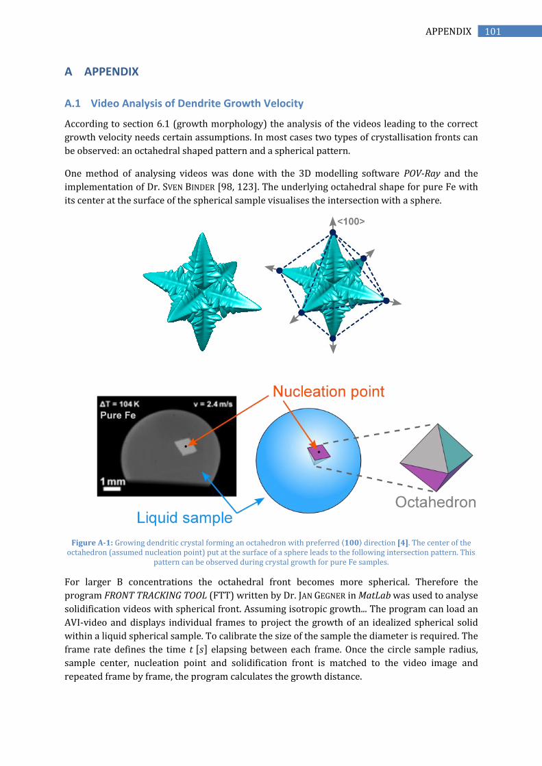
101 APPENDIX
A APPENDIX
A.1 Video Analysis of Dendrite Growth Velocity
According to section 6.1 (growth morphology) the analysis of the videos leading to the correct
growth velocity needs certain assumptions. In most cases two types of crystallisation fronts can
be observed: an octahedral shaped pattern and a spherical pattern.
One method of analysing videos was done with the 3D modelling software POV-Ray and the
implementation of Dr. SVEN BINDER [98, 123]. The underlying octahedral shape for pure Fe with
its center at the surface of the spherical sample visualises the intersection with a sphere.
Figure A-1: Growing dendritic crystal forming an octahedron with preferred ⟨𝟏𝟎𝟎⟩ direction [4]. The center of the octahedron (assumed nucleation point) put at the surface of a sphere leads to the following intersection pattern. This
pattern can be observed during crystal growth for pure Fe samples.
For larger B concentrations the octahedral front becomes more spherical. Therefore the
program FRONT TRACKING TOOL (FTT) written by Dr. JAN GEGNER in MatLab was used to analyse
solidification videos with spherical front. Assuming isotropic growth... The program can load an
AVI-video and displays individual frames to project the growth of an idealized spherical solid
within a liquid spherical sample. To calibrate the size of the sample the diameter is required. The
frame rate defines the time 𝑡 [𝑠] elapsing between each frame. Once the circle sample radius,
sample center, nucleation point and solidification front is matched to the video image and
repeated frame by frame, the program calculates the growth distance.

102 APPENDIX
The plot of the data represents the growth distance 𝑠 [𝑚𝑚] on the y-axis against time 𝑡 [𝑠] on the
x-axis. The slope 𝑚 [𝑚𝑚/𝑠] of the linear regression line is the growth velocity 𝑣 [𝑚𝑚/𝑠] which is
defined by:
𝑚 =∑ (𝑥𝑖 − �̅�)(𝑦𝑖 − �̅�)𝑛𝑖=1
∑ (𝑥𝑖 − �̅�)2𝑛
𝑖=1
,
where �̅�, �̅� are the mean values and 𝑥𝑖, 𝑦𝑖 each data point. The intercept 𝑏 = �̅� − 𝑚�̅� guarantees
that the distance from each data point to the line squared is minimized. This simple linear
regression line �̅� = 𝑚�̅� + 𝑏. least squares regression.
Figure A-2 shows a screenshot of the FFT program as example for a spherical front. The
diameter of the sample is 6.7 𝑚𝑚 and the high-speed video camera recorded with a framerate of
30,000 𝑓𝑝𝑠. After calibrating the sample diameter, the growth front and its center was stepwise
selected for each frame. The growth velocity plotted as the slope of growing radius per time
which is about 13.4 𝑚/𝑠 for this example using 10 frames of solidification.
Figure A-2: Screenshot of the program Front Tracking Tool (FFT)

103 BIBLIOGRAPHY
BIBLIOGRAPHY
[1] M. Rappaz and W. Kurz, “Dendrites solidified by computer,” Nature, vol. 375, p. 103 pp.,
1995.
[2] M. Asta, C. Beckermann, A. Karma, W. Kurz, R. Napolitano, M. Plapp, G. Purdy, M. Rappaz
and R. Trivedi, “Solidification microstructures and solid-state parallels: Recent
developments, future directions,” Acta Materialia, vol. 57, no. 146, pp. 941-971, 2009.
[3] D. M. Herlach, “Containerless Undercooling and Solidification of Pure Metals,” Annual
Review of Material Science, vol. 21, pp. 23-44, 1991.
[4] T. Haxhimali, A. Karma, F. Gonzales and M. Rappaz, “Orientation selection in dendritic
evolution,” Nature Materials, vol. 5, pp. 660-664, 2006.
[5] S. Binder, M. Kolbe, S. Klein and D. M. Herlach, “Solidification of tetragonal Ni2B from the
undercooled melt,” Europhysics Letters, vol. 97, no. 3, 2012.
[6] T. B. Cameron and J. E. Morral, Metallurgical Transactions, vol. 17, no. A, pp. 1481-1483,
1986.
[7] M. Palumbo, G. Cacciamani, E. Bosco and M. Baricco, “Thermodynamic Analysis of Glass
Formation in Fe-B System,” Calphad, vol. 25, no. 4, pp. 625-637, 2001.
[8] C. Karrasch, T. Volkmann, J. Valloton, M. Kolbe and D. M. Herlach, “Bent Dendrite Growth in
Undercooled Fe-B Alloy Melts,” IOP Conference Series: Material Science and Engineering,
submitted 2014.
[9] R. W. Hyers, Meas. Sci. Technol., no. 16, pp. 394-401, 2005.
[10] J. A. Dantzig and M. Rappaz, SOLIDIFICATION, Lausanne, Switzerland: EPFL Press, 2009.
[11] D. Herlach, P. Galenko and D. Holland-Moritz, METASTABLE SOLIDS FROM
UNDERCOOLED MELTS, Amsterdam, London: Elsevier, 2007.
[12] D. Turnbull, “Formation of crystal nuclei in liquid metals,” Journal of Applied Physics, vol.
21, pp. 1022-1028, 1950.
[13] R. R. Hultgren, Selected Values of the Thermodynamic Properties of Binary Alloys, Ohio:
American Society for Metals, 1973.
[14] M. Volmer and A. Weber, “Keimbildung in gesättigten Gebilden,” Zeitschrift für
physikalische Chemie, vol. 119, pp. 277-301, 1926.
[15] R. Becker and W. Döring, “Kinetische Behandlung der Keimbildung in übersättigten
Dämpfen,” Annalen der Physik, vol. 416, no. 8, pp. 719-752, 1935.

104 BIBLIOGRAPHY
[16] D. Turnbull and J. C. Fisher, “Rate of Nucleation in Condensed Systems,” Journal of
Chemical Physics, vol. 17, no. 71, 1949.
[17] R. Becker, “On the Formation of Nuclei during Precipitation,” Proceedings of the Physical
Society, vol. 52, pp. 71-76, 1940.
[18] M. Volmer, “Über Keimbildung und Keimwirkung als Spezialfälle der heterogenen
Katalyse,” Zeitschrift für Elektrochemie und angewandte physikalische Chemie, vol. 35, no. 9,
pp. 555-561, 1929.
[19] C. V. Thompson, Harvard Universiy: Ph.D. Thesis, 1979.
[20] C. V. Thompson and F. Spaepen, “Homogeneous Crystal Nucleation in Binary Metallic
Melts,” Acta Metallurgica, vol. 31, pp. 2021-2027, 1983.
[21] F. Spaepen, “Structual Model for the Solid-Liquid Interface in Mono-Atomic Systems,” Acta
Met., vol. 23, pp. 729-743, 1975.
[22] F. Spaepen and R. B. Meyer, “The Surface Tension in a Structural Model for the Solid-Liquid
Interface,” Scripta Metallurgica, vol. 10, pp. 257-263, 1976.
[23] F. C. Frank, “Supercooling of Liquids,” Proc. Roy. Soc. Lond., vol. A 215, pp. 43-46, 1952.
[24] D. R. Nelson and F. Spaepen, “Polytetrahedral Order in Condensed Matter,” Solid State
Physics, vol. 42, pp. 1-90, 1989.
[25] W. E. McMullen and D. W. Oxtoby, “A Theoretical Study of the Hard Sphere Fluid-Solid
Interface,” J. Chem. Phys., vol. 88, pp. 1967-1975, 1988.
[26] D. Holland-Moritz, Ordnungsphänomene, fest-flüssig Grenzflächen und Phasenselektion in
unterkühlten Metallschmelzen, Ruhr-Universität Bochum: Habilitationsschrift, 2003.
[27] Z. Jian, K. Kuribayashi and W. Jie, “Solid-liquid Interface Energy of Metals at Melting Point
and Undercooled State,” Materials Transactions, vol. 42, no. 4, pp. 721-726, 2002.
[28] J. W. Christian, The Theory of Transformations in Metals and Alloys, Oxford: Pergamon,
1975.
[29] A. A. Chernov, Modern Chrystallography III, vol. 36, Berlin: Springer, 1984.
[30] H. A. Wilson, “On the velocity of solidification and viscosity of supercooled liquids,” Philos.
Mag., vol. 50, pp. 238-250, 1900.
[31] J. Frenkel, “Note on a relation between the speed of crystallization and viscosity,” Phys. Z.
Sowj., vol. 1, pp. 498-500, 1932.
[32] K. A. Jackson, “The Interface Kinetics of Crystal Growth Processes,” Interface Science, vol.
10, pp. 159-169, 2002.

105 BIBLIOGRAPHY
[33] W. Klement, R. H. Willens and P. Duwez, “Non-Crystalline Structure in Solidified Gold-
Silicon Alloys,” Nature, vol. 187, no. 4740, p. 869–870, 1960.
[34] M. Telford, “The Case for Bulk Metallic Glass,” Materials Today, vol. 7, no. 3, pp. 36-43,
2004.
[35] Y. H. Liu, G. Wang, R. J. Wang, D. Q. Zhao, M. X. Pan and W. H. Wang, “Super Plastic Bulk
Metallic Glasses at Room Temperature,” Science, vol. 315, no. 5817, pp. 1385-1388, 2007.
[36] H. Guo, P. F. Yan and Y. B. Wang, “Tensile Ductility and Necking of Metallic Glass,” Nature
Materials, vol. 6, no. 10, pp. 735-739, 2007.
[37] D. C. Hofmann, “Bulk Metallic Glasses and Their Composites: A Brief History of Diverging
Fields,” Journal of Materials, pp. 1-8, 2013.
[38] M. J. Aziz, “Model for Solute Redistribution During Rapid Solidification,” Journal of Applied
Physics, vol. 53, pp. 1158-1168, 1982.
[39] M. J. Aziz and T. Kaplan, “Continuous Growth Model for Alloy Solidification,” Acta
Metallurgica, vol. 36, pp. 2335-2347, 1988.
[40] W. Kurz and D. J. Fisher, Fundamentals of Solidification, Lausanne: Trans Tech
Publications, 1989.
[41] K. Eckler, Dendritisches Wachstum in unterkuehlten Metallschmelzen, Ruhr-Universität
Bochum: Dissertation, 1992.
[42] P. K. Galenko, “Solute trapping and diffusionless solidification in a binary system,” Phys.
Rev. E, no. 76, 2007.
[43] J. J. Hoyt, M. Asta and A. Karma, “Atomistic Simulations of Solute Trapping and Solute
Drag,” in Solidification of Containerless Undercooled Melts, Weinheim, Wiley-VCH, 2012, pp.
363-380.
[44] P. K. Galenko and D. A. Danilov, “Local Nonequilibrium Effect on Rapid Dendritic Growth in
a Binary Alloy Melt,” Pysics Letters A, vol. 235, pp. 271-280, 1997.
[45] P. K. Galenko and D. A. Danilov, “Model for Free Dendritic Alloy Growth under Interfacial
and Bulk Phase Nonequilibrium Conditions,” Journal of Crystal Growth, vol. 197, pp. 992-
1002, 1999.
[46] J. Lipton, W. Kurz and R. Trivedi, “Rapid Dendrite Growth in Undercooled Alloys,” Acta
Metallurgica, vol. 35, no. 4, pp. 957-964, 1987.
[47] J. Brillo, A. I. Pommrich and A. Meyer, “Relation between Self-Diffusion and Viscosity in
Dense Liquids: New Experimental Results from Electrostatic Levitation,” Physical Review
Letters, vol. 107, no. 165902, pp. 5902-1-4, 2011.

106 BIBLIOGRAPHY
[48] A. Kerrache, J. Horbach and K. Binder, “Molecular Dynamics Computer Simulation of
Crystal Growth and Melting in Al50Ni50,” Europhys. Lett., vol. 81, pp. 58001:1 - 6, 2008.
[49] S. C. Huang and M. E. Glicksman, “Overview 12: Fundamentals of Dendritic Solidification-II.
Steady-State Tip Growth,” Acta Metallurgica, vol. 29, pp. 701-715, 1981.
[50] D. E. Temkin, “Growth Velocity of a Needle Crystal in a Supercooled Melt,” Dokl. Akad. Nauk
SSSR , vol. 132, pp. 1307-1310, 1960.
[51] J. S. Langer and H. Müller-Krumbhaar, “Stability Effects in Dendritic Crystal Growth,”
Journal of Crystal Growth, vol. 42, pp. 11-14, 1977.
[52] J. S. Langer and H. Müller-Krumbhaar, “Theory of Dendritic Growth-I. Elements of a
Stability Analysis,” Acta Metallurgica, vol. 26, pp. 1681-1687, 1978.
[53] B. Caroli, C. Caroli, B. Roulet and J. S. Langer, “Solvability Condition for Needle Crystals at
Large Undercooling in a Nonlocal Model of Solidification,” Physical Review A, vol. 33, no. 1,
pp. 442-452, 1986.
[54] D. A. Kessler and H. Levine, “Velocity Selection in Dendritic Growth,” Physical Review B, vol.
33, no. 11, pp. 7867-7870, 1986.
[55] M. Ben Amar, “Dendritic Growth Rate at Arbitary Undercooling,” Physical Review A, vol. 41,
no. 4, pp. 2080-2092, 1990.
[56] A. Barbieri, D. C. Hong and J. S. Langer, “Velocity Selection in the Symmetric Model of
Dendritic Crystal Growth,” Physical Review A, vol. 1987, pp. 1802-1808, 35.
[57] D. V. Alexandrov and P. K. Galenko, “Selection criterion of stable dendritic growth at
arbitary Péclet numbers with convection,” Phys. Rev. E, vol. 87, no. 6, pp. 062403:1-
062403:5, 2013.
[58] J.-H. Jeong, N. Goldenfeld and J. A. Dantzig, “Phase field model for three-dimensional
dendritic growth with fluid flow,” Phys. Rev. E, no. 64, 2001.
[59] P. K. Galenko, O. Funke, J. Wang and D. M. Herlach, “Kinetics of Dendritic Growth under the
Influence of Convective Flow in Solidification of Undercooled Droplets,” Materials Science
Engineering A, pp. 375-377, 2004.
[60] P. Galenko, S. Binder and G. J. Ehlen, “Forced Flow Effect on Dendritic Growth Kinetics in a
Binary Non-Isothermal System,” in Solidification of Containerless Undercooled Melts,
Weinheim, Wiley-VCH, 2012, pp. 349-362.
[61] P. Bouissou and P. Pelcé, “Effect of a Forced Flow on Dendritic Growth,” Phys. Rev. A, no.
40, p. 6673–6680, 1989.
[62] K. A. Jackson and J. D. Hunt, Trans. Metall Soc. AIME, vol. 236, pp. 1129-1142, 1966.
[63] W. Kuang, C. Karrasch, H. Wang, F. Liu and D. M. Herlach, “Eutectic Dendrite Growth in

107 BIBLIOGRAPHY
Undercooled Fe83B17 Alloy: Experiments and Modeling,” Scripta Materialia, vol. 105, pp.
34-37, 2015.
[64] W. Kurz and D. J. Fisher, “Dendrite Growth in Eutectic Alloys: The Coupled Zone,”
International Materials Reviews, vol. 24, no. 1, pp. 177-204, 1979.
[65] A. Karma and A. Sarkissian, “Morphological Instabilities of Lamellar Eutectics,”
Metallurgical Materials and Transactions A, vol. 27, no. 3, pp. 635-656, 1996.
[66] H. Walker, S. Liu, J. H. Lee and R. Trivedi, “Eutectic Growth in Three Dimensions,”
Metallurgical and Materials Transactions A, vol. 38, no. 7, pp. 1417-1425, 2007.
[67] S. Akamatsu, S. Bottin-Rousseau and G. Faivre, “Determination of the Jackson–Hunt
Constants of the In–In2Bi Eutectic Alloy based on In Situ Observation of its Solidification
Dynamics,” Acta Materialia, vol. 59, pp. 7586-7591, 2011.
[68] R. Trivedi, P. Magnin and W. Kurz, “Theory of Eutectic Growth under Rapid Solidification
Conditions,” Acta Metallurgica, vol. 35, no. 4, pp. 971-980, 1987.
[69] W. Kurz and R. Trivedi, “Eutectic Growth under Rapid Solidification Condition,” Metall.
Trans., vol. 22, pp. 3051-3057, 1991.
[70] H. F. Wang, F. Liu, Z. Chen, G. C. Yang and Y. H. Zhou, “Analysis of Non-Equilibrium
Dendrite Growth in Bulk Undercooled Alloy Melt: Model and Application,” Acta Materialia,
vol. 55, pp. 497-506, 2007.
[71] H. F. Wang, F. Liu, Z. Chen, W. Yang, G. C. Yang and Y. H. Zhou, “Effect of Non-Linear
Liquidus and Solidus in Undercooled Dendrite Growth: A Comparative Study in Ni–0.7
at.% B and Ni–1 at.% Zr Systems”.
[72] B. Wei, D. Herlach, B. Feuerbacher and F. Sommer, “Dendritic and Eutectic Solidification of
Undercooled Co-Sb Alloys,” Acta Metallurgica & Materialia, vol. 41, pp. 1801-1809, 1993.
[73] L. Liu, J. F. Li and Y. H. Zhou, “Solidification Interface Morphology Pattern in Undercooled
Co-24.0 at% Sn Eutectic Melt,” Acta Materialia, vol. 59, pp. 5558-5567, 2011.
[74] R. Goetzinger, M. Barth and D. M. Herlach, “Physical Mechanism of Formation of the
Anomalous Eutectic Structure in Ni-Si, Co-Sb and Ni-Al-Ti Alloys,” Acta Materialia, vol. 46,
pp. 1647-1655, 1998.
[75] J. F. Li and Y. H. Zhou, “Eutectic Growth in Bulk Undercooled Melts,” Acta Materialia, vol.
53, no. 8, pp. 2351-2359, 2005.
[76] P. K. Galenko and D. M. Herlach, “Diffusionless Crystal Growth in Rapidly Solidifying
Eutectic Systems,” Physical Review Letters , vol. 96, p. 150602, 2006.
[77] H. F. Wang, F. Liu and D. M. Herlach, “On the Solution of Solute Diffusion during Eutectic
Growth,” Journal of Crystal Growth, vol. 389, pp. 68-73, 2014.

108 BIBLIOGRAPHY
[78] H. F. Wang, F. Liu and D. M. Herlach, “Kinetics of Triple-Junctions in Eutectic Solidification:
A Sharp Interface Model,” Journal of Materials Science, vol. 50, pp. 176-188, 2015.
[79] H. F. Wang, F. Liu, H. M. Zhai and K. Wang, “Application of the Maximal Entropy Production
Principle to Rapid Solidification: A Sharp Interface Model,” Acta Materialia, vol. 60, pp.
1444-1454, 2012.
[80] H. F. Wang, F. Liu and D. M. Herlach, “Modeling the Growth Kinetics of a Multicomponent
Stoichometric Compound,” J. Materials Science, vol. 49, pp. 1537-1543, 2014.
[81] G. P. Ivantsov, Dokl. Akad. Nauk. SSSR., vol. 58, p. 567, 1947.
[82] P. K. Galenko, S. Reutzel, D. M. Herlach, D. Danilov and B. Nestler, “Modelling of Dendritic
Solidification in Undercooled Dilute Ni-Zr Melts.,” Acta Materialia, vol. 55, p. 6834–6842,
2007.
[83] P. K. Galenko, S. Reutzel, D. M. Herlach, S. G. Fries, I. Steinbach and M. Apel, “Dendritic
Solidification in Undercooled Ni–Zr–Al Melts: Experiments and Modelling,” Acta
Materialia, vol. 57, p. 6166–6175, 2009.
[84] G. Lohöfer and J. Piller, “The new ISS electromagnetic levitation facility: MSL - EML,”
Proceedings 40th AIAA Aerospace Sciences Meeting & Exhibit, 2002.
[85] Novespace, “Multimedia,” Novespace, 2007. [Online]. Available:
http://www.novespace.fr/en,home,download.html. [Accessed 11 2015].
[86] A. Gerst, “twitter.com: 3-2-1 GO! Switching on power to Electromagnetic Levitator #EML -
finding alloys on #ISS for the engine of the future,” ESA, 05 11 2014. [Online]. Available:
https://twitter.com/Astro_Alex/status/529930334960640000?nav=true. [Accessed 09
11 2015].
[87] NASA, “DLR,” NASA, [Online]. Available:
http://www.dlr.de/next/desktopdefault.aspx/tabid-7443/12421_read-30013/. [Accessed
11 2015].
[88] H. Yasuda, I. Ohnaka, Y. Ninomiya, R. Ishii, S. Fujita and K. Kishio, “Levitation of Metallic
Melt by Using the Simultaneous Imposition of the Alternating and Static Magnetic Fields,”
Journal of Crystal Growth, vol. 260, pp. 475-485, 2004.
[89] H. W. Kui, A. L. Greer and D. Turnbull, “Formation of Bulk Metallic Glass by Fluxing,”
Applied Physics Letters, vol. 45, no. 6, pp. 615-616, 1984.
[90] J. Wu, T. J. Piccone, Y. Shiohara and M. C. Flemings, “Dendritic Growth of Undercooled
Nickel-Tin: Part I,” Metallurgical Transactions A, vol. 18A, pp. 915-924, 1987.
[91] A. Yeckel and J. J. Derby, “Dynamics of Three-Dimensional Convection in Microgravity
Crystal Growth: g-Jitter with Steady Magnetic Fields,” Journal of Crystal Growth, vol. 263,
pp. 40-52, 2004.

109 BIBLIOGRAPHY
[92] Y. K. Zhang, J. Gao, D. Nagamatsu, T. Fukuda, H. Yasuda, M. Kolbe and J. C. He, “Reduced
Droplet Coarsening in Electromagnetically Levitated and Phase-Seperated Cu-Co Alloys by
Imposition of a Static Magnetic Field,” Scripta Materialia, vol. 59, pp. 1002-1005, 2008.
[93] E. Boehm-Courjault, F. Gonzales, A. Jacot, F. Kohler, A. Mariaux, C. Niederberger, M. A.
Salgado-Ordorica and M. Rappaz, “EBSD: A Powerful Microstructure Analysis Technique in
the Field of Solidification,” Journal of Microscopy, vol. 233, pp. 160-169, 2009.
[94] J. Berlin, “Analysis of Boron with Energy Dispersive X-ray Spectrometry,” Imaging &
Microscopy, vol. 13, no. 2, pp. 19-21, 2011.
[95] H. Okamoto, “B-Fe (boron-iron),” Journal of Phase Equilibria and Diffusion, vol. 25, no. 3,
pp. 297-298, 2004.
[96] A. M. Mullis, “Growth induced dendritic bending and rosette formation during
solidification in a shearing low,” Acta Materialia, vol. 47, pp. 1783-1789, 1999.
[97] M. Yamaguchi and C. Beckermann, “Simulation of solid deformation during solidification:
Compression of a single dendrite,” Acta Materialia, vol. 61, pp. 4053-4065, 2013.
[98] S. Binder, Dissertation: Undercooling and Solidification of tetragonal Ni2B under different
convective flow conditions, Bochum, 2010.
[99] L. Liu, J. F. Li and Y. H. Zhou, “Solidification Interface Morphology Pattern in the
undercooled Co-24.0 at.% Sn Eutectic Melt,” Acta Materialia, vol. 59, pp. 5558-5567, 2011.
[100] L. Gánásy, T. Pusztai, J. A. Warren, J. F. Douglas, T. Börzsönyi and V. Ferreiro, “Growth of
‘dizzy dendrites’ in a random field of foreign particles,” Nature Materials, vol. 2, pp. 92-96,
2003.
[101] B. T. Bassler, W. H. Hofmeister and R. J. Bayuzick, “The Solidification Velocity of Pure
Nickel,” Materials Science and Engineering A, vol. 342, pp. 80-92, 2003.
[102] P. M. Nasch, M. H. Manghnani and R. A. Secco, “Sound Velocity Measurements in Liquid
Iron by Ultrasonic Interferometry,” Journal of Geophysical Research, vol. 99, no. B3, p.
4285–4291 , 1994.
[103] R. S. Hixson, M. A. Winkler and M. L. Hodgdon, “Sound Speed and Thermophysical
Properties of Liquid Iron and Nickel,” Physical Review B, vol. 42, no. 10, pp. 6485-6491,
1990.
[104] T. Schenk, D. Holland-Moritz, V. Simonet, R. Belissent and D. M. Herlach, “Icosahedral
Short-Range Order in Deeply Undercooled Metallic Melts,” Physical Review Letters, vol. 89,
no. 7, pp. 61:20-25, 2002.
[105] Y. Ashkenazy and R. S. Averback, “Kinetic Stages in the Crystallization of Deeply
Undercooled Body-Centered-Cubic and Face-Centered-Cubic metals,” Acta Materialia, vol.
58, pp. 524-530, 2010.

110 BIBLIOGRAPHY
[106] Y. Mu, A. Houk and X. Song, “Anisotropic Interfacial Free Energies of the Hard-Sphere
Crystal-Melt Interfaces,” Journal of Physical Chemistry B, vol. 109, p. 6500–6504, 2005.
[107] R. Hyers, D. M. Matson, K. F. Kelton, D. Holland-Moritz and T. Volkmann, “Fluid-Flow
Effects on Phase Selection and Nucleation in Undercooled Liquid Metals,” Journal of
Physics: Conference Series, vol. 327, pp. 012013:1-7, 2011.
[108] J. Gao, M. Han, A. Kao, K. Pericleous, D. V. Alexandrov and P. K. Galenko, “Dendritic Growth
Velocities in an Undercooled Melt of Pure Nickel under Static Magnetic Fields: A Test of
Theory with Convection,” Acta Materialia, vol. 103, pp. 184-191, 2016.
[109] D. V. Alexandrov and P. K. Galenko, “Dendrite Growth under Forced Convection: Analysis
Methods and Experimental Tests,” Physics Uspekhi, vol. 57, no. 8, pp. 771-786, 2014.
[110] K. Eckler, R. F. Cochrane, D. M. Herlach and B. Feuerbacher, “Evidence for a transition from
diffusion-controlled to thermally controlled solidification in metallic alloys,” Physical
Review B, vol. 45, no. 9, pp. 5019-5022, 1992.
[111] K. Eckler, D. M. Herlach, R. G. Hamerton and A. L. Greer, “Dendrite Growth Velocities in
Highly Undercooled, Dilute Ni-C melts,” Material Science and Engineering, vol. A, no. 133,
pp. 730-733, 1991.
[112] C. Yang, F. Liu, G. Yang and Y. Zhou, “Structure evolution upon non-equilibrium
solidification of bulk undercooled Fe-B system,” Journal of Crystal Growth, vol. 311, pp.
404-412, 2009.
[113] M. Palumbo, G. Cacciamani, E. Bosco and M. Baricco, “Thermodynamic Analysis of Glass
Formation in Fe-B System,” Calphad, vol. 25, no. 4, pp. 625-637, 2001.
[114] C. Yang, F. Liu, G. Yang, Y. Chen, N. Liu and Y. Zhou, “Microstructure and Phase Selection in
Bulk Undercooled Fe–B Eutectic Alloys,” Journal of Alloys and Compounds, vol. 441, no. 1-2,
pp. 101-106, 2007.
[115] L. Battezzati, C. Antonione and M. Baricco, “Undercooling of Ni-B and Fe-B alloys and their
metastable phase diagrams,” Journal of Alloys and Compounds, vol. 247, pp. 164-171, 1997.
[116] T. V. Rompaey, K. C. H. Kumar and P. Wollants, “Thermodynamic Optimization of the B–Fe
System,” Journal of Alloys and Compounds, vol. 334, p. 173.181, 2002.
[117] R. Trivedi and W. Kurz, “Modeling of Solidification Microstructures in Concentrated
Solutions and Intermetallic Systems,” Matallurgical Transactions A, vol. 21 A, pp. 1113-
1118, 1990.
[118] C. Yang, J. Gao, Y. K. Zhang, M. Kolbe and D. M. Herlach, “New Evidence for the Dual Origin
of Anomalous Eutectic Structures in Undercooled Ni-Sn Alloys: In Situ Observations and
EBSD Characterization,” Acta Materialia 59, vol. 59, pp. 3915-3926, 2011.
[119] N. Wang, Y. E. Kalay and R. Trivedi, “Eutectic-to-Metallic Glass Transition in the Al–Sm

111 BIBLIOGRAPHY
System,” Acta Materialia, vol. 59, pp. 6604-6619, 2011.
[120] R. Trivedi and N. Wang, “Theory of Rod Eutectic Growth Under Far-From-Equilibrium
Conditions: Nanoscale Spacing and Transition to Glass,” Acta Materialia, vol. 60, pp. 3140-
3152, 2012.
[121] I. Steinbach, “Phase-Field Models in Materials Science,” Modelling and Simulation in
Materials Science and Engineering, vol. 17, pp. 073001:1-31, 2009.
[122] R. Trivedi and W. Kurz, “Casting and Solidification,” in Materials Processing Handbook,
Boca Raton, CRC Press, 2007, pp. 16:1-18.
[123] D. M. Herlach and D. M. Matson, Solidification of Containerless Undercooled Melts,
Weinheim: Wiley-VCH, 2012.
[124] D. Y. Sun and M. Asta, “Crystal-Melt Interfacial Free Energies and Mobilities in fcc and bcc
Fe,” Physical Review B, vol. 69, 2004.
[125] J.-. H. Jeong, N. Goldenfeld and J. A. Dantzig, “Phase Field Model for Three-Dimensional
Dendritic Growth with Fluid Flow,” PHYSICAL REVIEW E, vol. 64, pp. 041602:1-14, 2001.
[126] M. Barth, F. Joo, B. Wei and D. M. Herlach, “Measurement of the enthalpy and specific heat
of undercooled nickel and iron melts,” Journal of Non-Crystalline Solids, pp. 398-401, 1993.
[127] O. Tolochko and J. Agren, “Thermodynamic Properties of Supercooled Fe-B Liquids - A
Theoretical and Experimental Study,” Journal of Phase Equilibria, vol. 21, no. 1, pp. 19-24,
2000.

112 Publication List
PUBLICATION LIST
The following publications are already published/submitted including results of this thesis with
permission of Prof. Dr. Dieter M. Herlach.
[SCRIPTA MATERIALIA] W. Kuang, C. Karrasch, H. Wang, F. Liu and D. M. Herlach, “Eutectic
Dendrite Growth in Undercooled Fe83B17 Alloy: Experiments and
Modeling,” Scripta Materialia, vol. 105, pp. 34-37, 2015.
[IOP] C. Karrasch, T. Volkmann, J. Valloton, M. Kolbe and D. M. Herlach,
“Bent Dendrite Growth in Undercooled Fe-B Alloy Melts,” IOP
Conference Series: Material Science and Engineering, accepted
2014.

113 Acknowledgments
ACKNOWLEDGMENTS
No man is an island,
Entire of itself, …
JOHN DONNE (1572-1631)
This thesis could not have been written without the help and support of others…
First of all, I want to thank my supervisor Prof. Dr. Dieter M. Herlach for his support and infinite patience. His experience and interest in the experimental investigations as well as discussions about modelling were extremely valuable and encouraging. He offered me the chance to work on this interesting topic and to join his group of excellent scientists. I am very thankful for the opportunity he offered me to present my scientific results in many international conferences all over the world. The participation in two parabolic flights were an awesome and unforgettable experience.
I am grateful to Prof. Dr. Kurt Westerholt to be the second referee.
I would like to thank Prof. Dr. Andreas Meyer for support and the opportunity to work at the Institute of Materials Physics in Space at the German Aerospace Center in Cologne.
I want to thank:
Dr. Thomas Volkmann as an advisor, for his help and support in experimental and theoretical questions.
Dr. Matthias Kolbe for taking SEM/EBSD images and fruitful discussions in life and science.
Dr. Jan Gegner for proofreading this thesis and using his MATLAB program to analyse videos and modelling dendrite growth velocities.
Dr. Jonas Valloton for many measurement sessions and a great time with him.
Dr. Stefan Klein for proofreading this thesis, his help and support.
Marcus Reinartz for investigations with the InfraRed-camera.
Prof. Dr. Haifeng Wang and his student Kuang Wangwang for cooperation in modelling and a lifelong treasure for me to visit Xi’An.
Prof. Dr. Jianrong Gao for the opportunity to visit and measure at the Northeastern University of Shenyang, very fruitful discussions and double checking my modelling results.
Dr. D. Holland-Moritz and Dr. P. Galenko for discussions and useful suggestions.
Raphael Kobold for being a colleague and good friend. Pierre-Yves for being a friend and office mate during our journey to become a PhD.
Ingeborg Parpart and Kim Prochnow to be the heart of our institute glueing all together.
Claudia Wulf for being an island of help and support in the ocean of RUB.
The workshop guys Matthias, Kosta, Horst and Ralf for their humor and supply of coffee in bad times.
Heliana Cardenas for her motivational friendship and proofreading for parts of this thesis.
Stefan Burggraf for being a friend in hard times, proofreading and support in sample preparation.
Simon Haßelmann for proofreading this thesis and being his best man.
This work was financially supported by the German Research Foundation DFG within contract HE1601/18 and the European Space Agency ESA under contract numbers 4200020277 and 4200014980.
Finally I would like to thank my family and friends for their support, love and never-ending patience to hear the words: “Sorry, I cannot join, I am about to finish and I have to finally work on my thesis.”
Special thanks to Dr. med. Karolina Jablonska for her love, support and infinite patience.

114 Curriculum Vitae
CURRICULUM VITAE
Name: Christian Karrasch
Date of Birth: 28.06.1982
Place of Birth: Bonn-Duisdorf, Germany
Nationality: German
08/88 – 06/92 Grundschule Finkenhof, Bonn Hardtberg
06/92 – 06/98 Realschule Hardtberg, Bonn
08/98 – 29/06/01 Abitur, Helmholtz Gymnasium, Bonn
11/01– 09/02 Wehrdienst
10/02 – 27/06/11 Diploma in Physics, Rheinische Friedrich-Wilhelms-Universität
Bonn. Diploma Thesis in the works of PD. Dr. R. Vianden at the
Helmholtz-Institute for Radiation and Nuclear Physics:
„Kristallgitterschäden durch hohe elektrische Stromdichten im III-
V-Halbleiter Galliumnitrid“
02/12 - PhD Student in Physics of the Institute for Experimental Physics IV
(Ruhr-Universität Bochum) of Prof. Dr. Dieter M. Herlach in
cooperation with the Institute of Materials Physics in Space,
German Aerospace Center (DLR) in Cologne