SOLID-STATE SINTERING SIMULATION: …bruchon/conferences/PinoMunoz_ECCOMAS2012.pdfSOLID-STATE...

European Congress on Computational Methodsin Applied Sciences and Engineering (ECCOMAS 2012)

J. Eberhardsteiner et.al. (eds.)Vienna, Austria, September 10-14, 2012

SOLID-STATE SINTERING SIMULATION: SURFACE, VOLUME ANDGRAIN-BOUNDARY DIFFUSIONS

Daniel Pino Munoz, Julien Bruchon, Francois Valdivieso and Sylvain Drapier

Centre Sciences des Materiaux et des Structures & LCG UMR CNRS 5146Ecole Nationale Superieure des Mines de Saint-Etienne

158 Cours Fauriel, 42023, Saint-Etienne, Francepino,bruchon,valdivie,[email protected]

Keywords: Sintering, Diffusion phenomena, Surface tension, Finite elements, Level-set meth-ods

Abstract. Within the general context of solid-state sintering process, this work presents anumerical modeling approach, at the grain scale, of ceramic grain packing consolidation. Typ-ically, the sintering process triggers several mass transport paths that are thermally activated:surface, grain boundary and volume diffusions. Including this physics into a high-performancecomputing framework would permit to gain precious insights about the driving mechanismswhich are seldom accessible at this scale.

In performing this kind of simulations, several challenges will be faced: the strong topolog-ical changes which appear during sintering simulation at the grains scale, the evolution of thestructure that is mainly driven by the surface tension phenomena through the Laplace’s law,and the mechanical properties of the grains which could, possibly, be different. The proposednumerical simulations are carried out within an Eulerian Finite Element framework and theLevel-Set method is used to cope with changes in the microstructure. The results obtained withthis numerical strategy are compared with success to the usual geometrical models.


1 INTRODUCTION

Sintering is one of the stages of the powder metallurgy manufacturing process. Sintering isused for the fabrications of high performances materials and parts in a wide -and still growing-range of domains. Since the 50’s a large amount of work has dedicated to the theoretical andexperimental study of this process. However the understanding of the underlying physical phe-nomena is still a field of active research. Diffusion phenomena are considered to be responsiblefor the microstructural evolution that takes place during sintering [8]. After the powder has beenshaped, under the heat action different diffusion mechanisms are thermally activated. Duringthe first stages of the process the necks between the particles are created. Necks continue todevelop allowing the open porosity to become closed, to finally end up by vanishing at the endof the sintering process.

Even if it is possible to distinguish at least six different diffusion mechanisms, this work ismainly concerned by the surface, volume and grain boundary diffusions, which are consideredto be the most important diffusion paths. Those diffusion mechanisms can be modeled by usingthe first Fick’s law. This law establishes a relationship between the matter flux j and the gradientof the chemical potential µ :

j = m∇µ (1)

where m is the mobility associated with the diffusion path considered. The chemical potentialmeasures the tendency to diffuse of a substance and its value depends on the region of theparticles that is being considered, e.g. surface, volume, grain-boundary, etc.

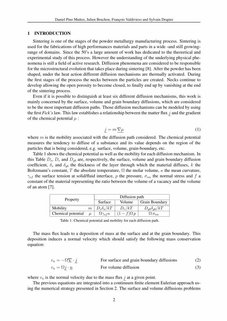
Table 1 shows the chemical potential as well as the mobility for each diffusion mechanism. Inthis Table Ds, Dv and Dgb are, respectively, the surface, volume and grain boundary diffusioncoefficient, δs and δgb the thickness of the layer through which the material diffuses, k theBoltzmann’s constant, T the absolute temperature, Ω the molar volume, κ the mean curvature,γsf the surface tension at solid/fluid interface, p the pressure, σnn the normal stress and f aconstant of the material representing the ratio between the volume of a vacancy and the volumeof an atom [7].

PropertyDiffusion path

Surface Volume Grain BoundaryMobility m Dsδs/kT Dv/kT Dgbδgb/kT

Chemical potential µ Ωγsfκ (1− f)Ω p Ωσnn

Table 1: Chemical potential and mobility for each diffusion path.

The mass flux leads to a deposition of mass at the surface and at the grain boundary. Thisdeposition induces a normal velocity which should satisfy the following mass conservationequation:

vn = −Ω∇ · j For surface and grain boundary diffusions (2)

vn = Ωj · n For volume diffusion (3)

where vn is the normal velocity due to the mass flux j at a given point.The previous equations are integrated into a continuum finite element Eulerian approach us-

ing the numerical strategy presented in Section 2. The surface and volume diffusions problems

2


are presented in Sections 3 and 4, respectively. In Section 5, the bases toward the sinteringsimulation by grain-boundary diffusion are stated. The results are presented in Section 7 andfinally the conclusions and perspectives are discussed in Section 8.

2 LEVEL-SET STRATEGY

Initially, the numerical strategy for the simulation of sintering by surface and volume diffu-sion is presented. The strategy for the simulation of sintering by grain-boundary diffusion isslightly different and will be developed in Section 5.

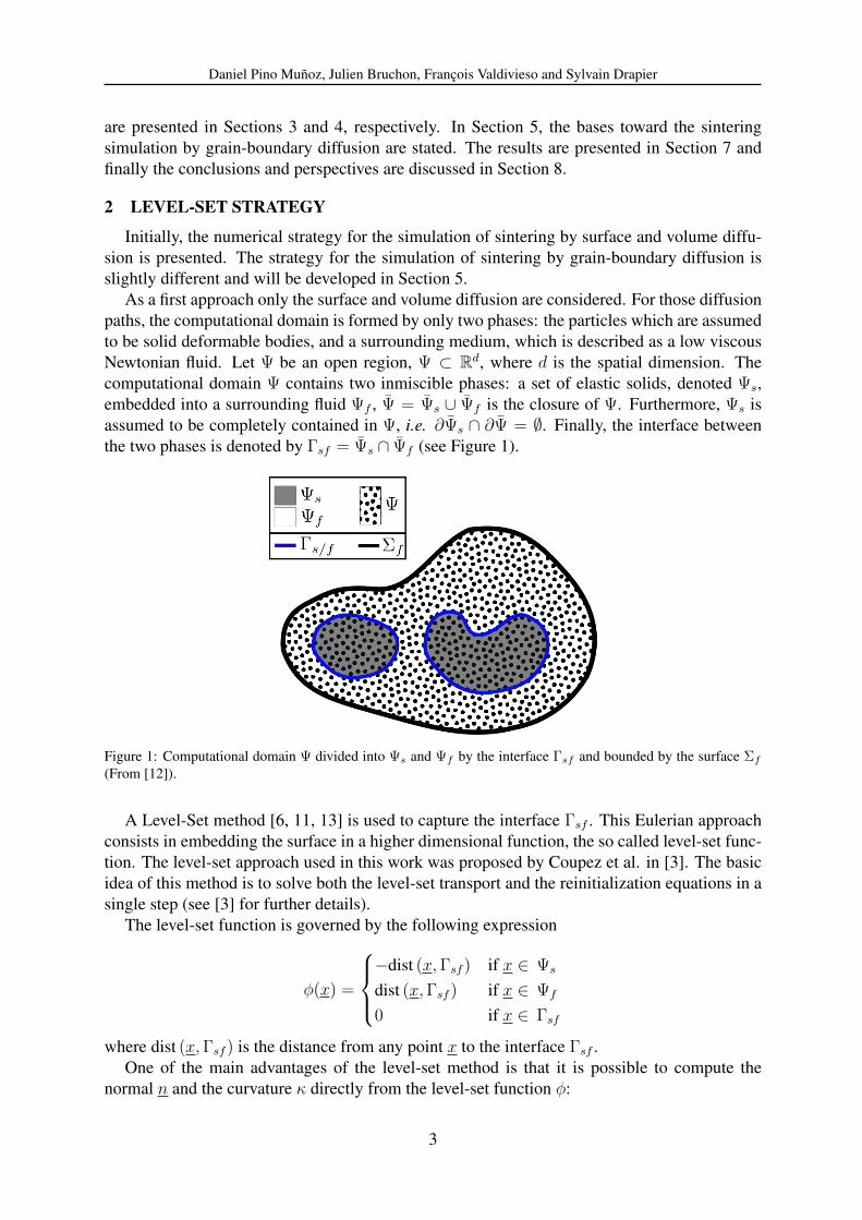
As a first approach only the surface and volume diffusion are considered. For those diffusionpaths, the computational domain is formed by only two phases: the particles which are assumedto be solid deformable bodies, and a surrounding medium, which is described as a low viscousNewtonian fluid. Let Ψ be an open region, Ψ ⊂ Rd, where d is the spatial dimension. Thecomputational domain Ψ contains two inmiscible phases: a set of elastic solids, denoted Ψs,embedded into a surrounding fluid Ψf , Ψ = Ψs ∪ Ψf is the closure of Ψ. Furthermore, Ψs isassumed to be completely contained in Ψ, i.e. ∂Ψs ∩ ∂Ψ = ∅. Finally, the interface betweenthe two phases is denoted by Γsf = Ψs ∩ Ψf (see Figure 1).

Figure 1: Computational domain Ψ divided into Ψs and Ψf by the interface Γsf and bounded by the surface Σf

(From [12]).

A Level-Set method [6, 11, 13] is used to capture the interface Γsf . This Eulerian approachconsists in embedding the surface in a higher dimensional function, the so called level-set func-tion. The level-set approach used in this work was proposed by Coupez et al. in [3]. The basicidea of this method is to solve both the level-set transport and the reinitialization equations in asingle step (see [3] for further details).

The level-set function is governed by the following expression

φ(x) =

−dist (x,Γsf ) if x ∈ Ψs

dist (x,Γsf ) if x ∈ Ψf

0 if x ∈ Γsf

where dist (x,Γsf ) is the distance from any point x to the interface Γsf .One of the main advantages of the level-set method is that it is possible to compute the

normal n and the curvature κ directly from the level-set function φ:

3


n =∇φ‖ ∇φ ‖

(4)

κ = ∇ · n (5)

In the classical level-set method, the level-set function φ is transported by solving the fol-lowing transport equation:

∂φ

∂t+∇φ · v = 0 (6)

In our case, the velocity v corresponds to the velocity due to the mass flux j and will becomputed by using equations (2) and (3). The Finite Elements Method is used to solve thePDEs presented in this work. The computational domain is discretized by using simplexes(triangles in 2D and tetrahedrals in 3D) with linear interpolations. In particular, when usingthe finite element method for the numerical treatment of equation (6), the Streamline upwindPetrov-Galerkin method (SUPG) is required.

3 SURFACE DIFFUSION

In Section 1, equations for modeling the surface diffusion were introduced. As showed inTable 1 the chemical potential on surface µs is proportional to the curvature κ, which means thatthe matter flux by surface diffusion js is proportional to the first derivative of the curvature js ∝∂κ. From equation (2), its associated velocity is proportional to the Laplacian of the curvaturevn ∝ ∂2κ. Furthermore, the curvature can be computed by using the Level-set function φ,but some difficulties will raise as the curvature κ is proportional to the second derivative of φ.In this case the normal velocity is proportional to the fourth derivative of φ: vn ∝ ∂4φ. Aclassical finite element computation of the normal velocity vn from φ would lead to unphysicaloscillations of the velocity field. As demonstrated by Bruchon et al. in [1], such oscillationsare greatly reduced by solving a mixed κ/∆κ formulation. The proposed mixed formulation ispresented in equations (7) and (8):

κt + ∇ ·(

∆t

A∇vtn

)= ∇ ·

(1

A∇φt

)(7)

vn ‖ ∇φt ‖ − C0∇ ·(Pφt · ∇κt

)= 0 (8)

where κt is the curvature at time t, ∆t is the time step, ∆t/A is a regularization parameter withA given by A =‖ ∇φt −∆t∇vt−∆t

n ‖, vtn is the normal velocity at the time t, φt is the level-setfunction at the time t, C0 is a constant containing the diffusion parameter of the material andPφt is the projection operator at time t given by: Pφt = I − n⊗ n.

Additionally, Bruchon et al [1] have shown that the velocity field obtained by solving equa-tions (7) and (8) leads to volume conservation.

4 VOLUME DIFFUSION

In this case, the matter flux is considered to be proportional to the gradient of the pressurep (Equation (3) and Table 1). This means that the mechanical problem should be solved inorder to compute the matter flux and therefore the associated normal velocity. At the particles

4


scale (microscopic scale), the effect of the surface tension phenomena can not be considered asnegligible. The numerical approach developed to solve the mechanical problem is presented inSection 4.1. According to equation (3), the normal velocity due to the volume diffusion is alsoproportional to the gradient of the pressure as it will be presented in Section 4.2.

4.1 Mechanical problem

The numerical approach developed to solve the mechanical problem is presented in [12].The inertia terms and the volume forces are neglected. The momentum conservation can beexpressed by the set of equations (9):

∇ · σ = 0 in Ψ (9a)σ · n = g in Σt (9b)v = vc in Σv (9c)[

σ · n]

Γsf= γsfκn in Γsf (9d)

where σ is the Cauchy stress tensor for the solid or the fluid. g is the stress vector on the outerboundary Σt, velocity v is equal to vc over Σv, [ • ]|Γsf

denotes a jump across the interface Γsf ,γsf is the surface tension coefficient and κ is the main curvature. The outer boundary of Ψ,Σf = ∂Ψ (showed in Figure 1), is divided into Σt and Σv where the Neumann and Dirichletboundary conditions are respectively applied.

For mass conservation issues, the formulation presented in this paper is a mixed formula-tion, the momentum conservation equation should be complemented with the mass conservationequation. Particles are assumed to have a linear elastic isotropic behavior:

σ = 2µε(u)−(

1− 2

3

µ

K

)pI (10a)

tr(ε(u)

)+

p

K= 0 (10b)

with p the pressure, u the displacement, µ the shear modulus, ε(u) = (∇u + t∇u)/2 thelinearized strain tensor, K the bulk modulus, tr (•) the trace operator and I the second orderidentity tensor.

The fluid is Newtonian incompressible:

σ = 2ηε(v)− pI (11a)

tr(ε(v)

)= 0 (11b)

where v the velocity, η the viscosity and ε(v) = (∇v + t∇v)/2 the strain rate tensor.The numerical method used to solve the mechanical problem (9) to (11), along with the

stabilization method is presented in [12]. The numerical treatment of the surface tension termis not straightforward within an Eulerian approach since there is no nodes over the interfaceΓsf . The Surface Local Reconstruction (SLR) method is used. However, since the interfaceΓsf is given by the zero isosurface of the level-set function (φ = 0), it is possible to locallyreconstruct the interface. This is the Surface Local Reconstruction (SLR) method used here:after the intersection between an element and the interface Γsf has been found, the surface

5


tension term can then be explicitly computed over this locally reconstructed surface. All thedetails concerning the numerical implementation of the method are presented in [12]. It isimportant to note that a stabilization method is required in order to satisfy the Ladyzenskaja-Babuska-Brezzi condition for P1/P1 elements. In this case, a multiscale stabilization method isused, specifically, the Algebraic Sub-Grid Scale stabilization (ASGS) method.

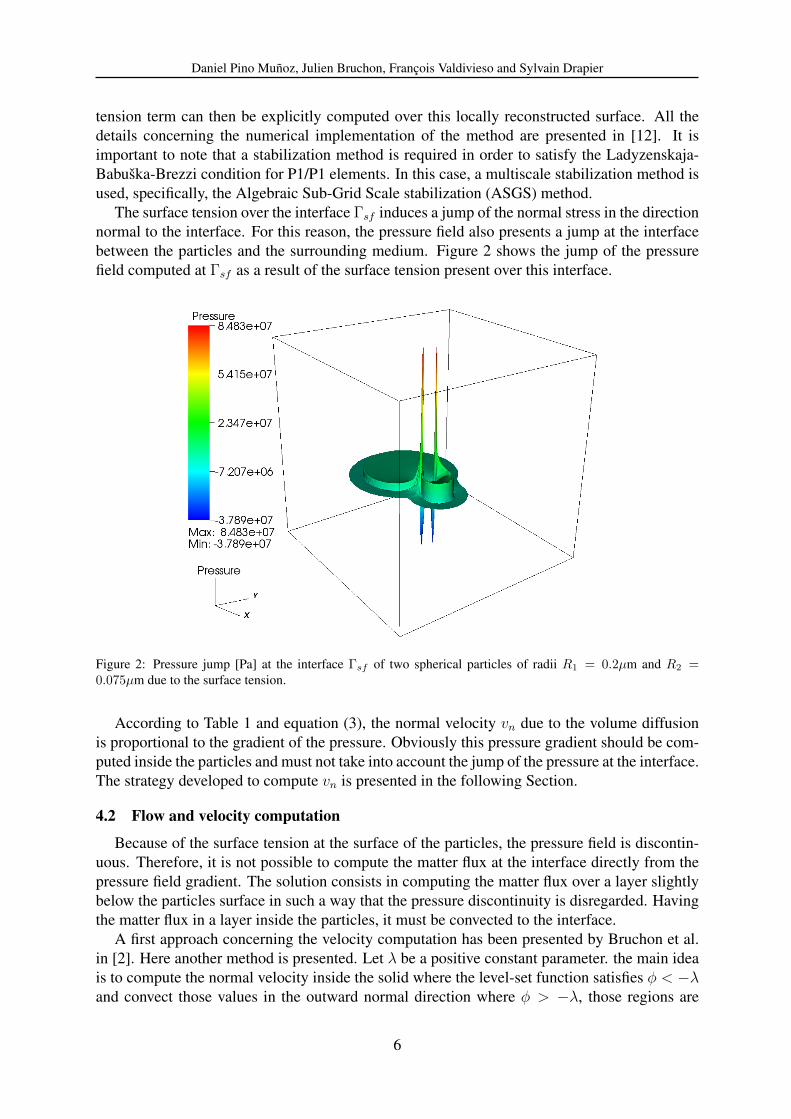
The surface tension over the interface Γsf induces a jump of the normal stress in the directionnormal to the interface. For this reason, the pressure field also presents a jump at the interfacebetween the particles and the surrounding medium. Figure 2 shows the jump of the pressurefield computed at Γsf as a result of the surface tension present over this interface.

Figure 2: Pressure jump [Pa] at the interface Γsf of two spherical particles of radii R1 = 0.2µm and R2 =0.075µm due to the surface tension.

According to Table 1 and equation (3), the normal velocity vn due to the volume diffusionis proportional to the gradient of the pressure. Obviously this pressure gradient should be com-puted inside the particles and must not take into account the jump of the pressure at the interface.The strategy developed to compute vn is presented in the following Section.

4.2 Flow and velocity computation

Because of the surface tension at the surface of the particles, the pressure field is discontin-uous. Therefore, it is not possible to compute the matter flux at the interface directly from thepressure field gradient. The solution consists in computing the matter flux over a layer slightlybelow the particles surface in such a way that the pressure discontinuity is disregarded. Havingthe matter flux in a layer inside the particles, it must be convected to the interface.

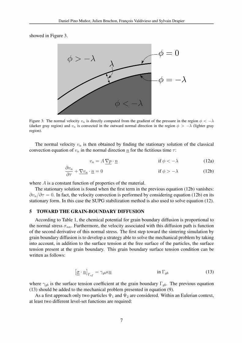
A first approach concerning the velocity computation has been presented by Bruchon et al.in [2]. Here another method is presented. Let λ be a positive constant parameter. the main ideais to compute the normal velocity inside the solid where the level-set function satisfies φ < −λand convect those values in the outward normal direction where φ > −λ, those regions are

6


showed in Figure 3.

Figure 3: The normal velocity vn is directly computed from the gradient of the pressure in the region φ < −λ(darker gray region) and vn is convected in the outward normal direction in the region φ > −λ (lighter grayregion).

The normal velocity vn is then obtained by finding the stationary solution of the classicalconvection equation of vn in the normal direction n for the fictitious time τ :

vn = A∇p · n if φ < −λ (12a)∂vn∂τ

+∇vn · n = 0 if φ > −λ (12b)

where A is a constant function of properties of the material.The stationary solution is found when the first term in the previous equation (12b) vanishes:

∂vn/∂τ = 0. In fact, the velocity convection is performed by considering equation (12b) en itsstationary form. In this case the SUPG stabilization method is also used to solve equation (12).

5 TOWARD THE GRAIN-BOUNDARY DIFFUSION

According to Table 1, the chemical potential for grain boundary diffusion is proportional tothe normal stress σnn. Furthermore, the velocity associated with this diffusion path is functionof the second derivative of this normal stress. The first step toward the sintering simulation bygrain boundary diffusion is to develop a strategy able to solve the mechanical problem by takinginto account, in addition to the surface tension at the free surface of the particles, the surfacetension present at the grain boundary. This grain boundary surface tension condition can bewritten as follows:

[σ · n

]Γsf

= γgbκn in Γgb (13)

where γgb is the surface tension coefficient at the grain boundary Γgb. The previous equation(13) should be added to the mechanical problem presented in equation (9).

As a first approach only two particles Ψ1 and Ψ2 are considered. Within an Eulerian context,at least two different level-set functions are required:

7


φ1(x) =

−dist (x,Γsf ) if x ∈ Ψ1

dist (x,Γsf ) if x /∈ Ψ1

0 if x ∈ ∂Ψ1

; φ2(x) =

−dist (x,Γsf ) if x ∈ Ψ2

dist (x,Γsf ) if x /∈ Ψ2

0 if x ∈ ∂Ψ2

In this way, the grain boundary Γgb is defined by the surface where φ1 ≡ 0 and φ2 ≡ 0.The solid/fluid interface Γsf is defined by the surface where one of the following conditions issatisfied:

• φ1 ≡ 0 and φ2 6= 0.

• φ1 6= 0 and φ2 ≡ 0

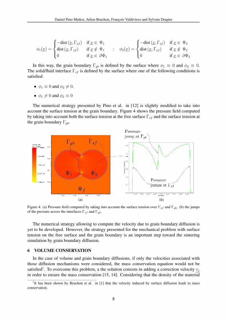
The numerical strategy presented by Pino et al. in [12] is slightly modified to take intoaccount the surface tension at the grain boundary. Figure 4 shows the pressure field computedby taking into account both the surface tension at the free surface Γsf and the surface tension atthe grain boundary Γgb.

Figure 4: (a) Pressure field computed by taking into account the surface tension over Γsf and Γgb. (b) the jumpsof the pressure across the interfaces Γsf and Γgb.

The numerical strategy allowing to compute the velocity due to grain boundary diffusion isyet to be developed. However, the strategy presented for the mechanical problem with surfacetension on the free surface and the grain boundary is an important step toward the sinteringsimulation by grain boundary diffusion.

6 VOLUME CONSERVATION

In the case of volume and grain boundary diffusions, if only the velocities associated withthose diffusion mechanisms were considered, the mass conservation equation would not besatisfied1. To overcome this problem, a the solution consists in adding a correction velocity vcin order to ensure the mass conservation [15, 14]. Considering that the density of the material

1It has been shown by Bruchon et al. in [1] that the velocity induced by surface diffusion leads to massconservation.

8


remains constant, the mass conservation leads to the conservation of the volume of the particles.This volume conservation is in agreement with the experimental results that can be found in theliterature.

In order to satisfy the volume conservation, the correction velocity is computed after eachtime step and is used to restore the initial volume of the structure. Let V0 be the initial volumeof the structure. After a time step, the volume at the time t (Vt) may be different from V0. Thecorrection velocity is assumed to be normal to the surface of the particles and is also assumedto be be constant over all the computational domain. Considering this, vc is given by:

vc =V0 − VtS∆t

n (14)

where S is the total area of the surface of the structure and ∆t is the time step. Finally, equation(14) is introduced into the convection equation (equation (6)) to recover the initial volume ofthe structure.

7 NUMERICAL RESULTS

All the developments have been implemented in the finite element library CimLib. CimLibis a highly parallel C++ library developed at Center for Material Forming (Mines ParisTech,CNRS UMR 7635) by the team of Professor Coupez [4]. As in [2], the simulations presented inthis work have been performed by using a mesh adaptation strategy aiming to obtain accurateresults while keeping a “reasonable” number of mesh elements. The mesh is refined over anarrow band around the surface of the particles, the detailed strategy is presented in [10]. Theelement size is computed as a function of the second derivative of a primal variable such asa filtered level-set function or the pressure field. This approach has successfully been appliedwithin the sintering simulation context by Bruchon et al. in [1, 2].

The material properties used in the following simulations correspond to the properties ofAlumina (Al2O3) and are summarized in Table 2.

Constant Value UnitsDsΩγsfδs/kT 1·10−7 m mol/sDvΩ (1− f) /kT 55.16 m mol/N s

K 260 GPaµ 156 GPaη 1e-3 Pa/sγsf 0.9 N/mΩ 8.55·10−6 m3/mol

Table 2: Material properties used.

7.1 Two particles sintering: surface and volume diffusions

The first step toward the simulation of sintering process at the particles scale consists instudying the growth of the neck formed between two particles during the early stages of sinter-ing. There exists different models attempting to predict the evolution of the radius of the neckX as a function of time. Those models2 are mainly based on some geometrical hypotheses of

2Also called power laws.

9


the evolution of the neck and the particles. In general those geometrical models can be writtenas follows: (

X(t)

r

)n= A t (15)

where r is the radius of the particles (supposed to remain constant) and A and n are parameterdepending on the radius of the particles and the diffusion path being considered. Even if thevalidity of these models is restricted to necks radii smaller than 30% of the radius of the par-ticles, they represent a very useful tool concerning the validation of the kinetic obtained frommore elaborated numerical approaches. For graphical purposes, equation (15) can be slightlymodified by introducing the dimensionless time t∗:(

X(t)

r

)n= A′ t∗ (16)

where A′ is a constant and no longer depends on the radius of the particles.

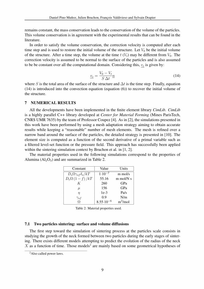
Figure 5: Growth by surface diffusion of the dimensionless neck radius X/r over the dimensionless time t∗ fordifferent values of r [1].

Figure 5 presents the evolution of the dimensionless radius X/r as a function of t∗ duringsintering by surface diffusion for particle radii between 0.1 and 2.5. According to Exner et al.[5], the exponent n on equation (16) ranges between 3 and 7 for surface diffusion, which is inagreement with the simulations performed here. The dashed line showed in Figure 5 (referredto as “Simulation, 1/7”) corresponds to the best fitting curve obtained by least-squares and forcomparison purposes, the line corresponding to n = 6 in equation (16) is also plotted (referredto as “1/6 law”).

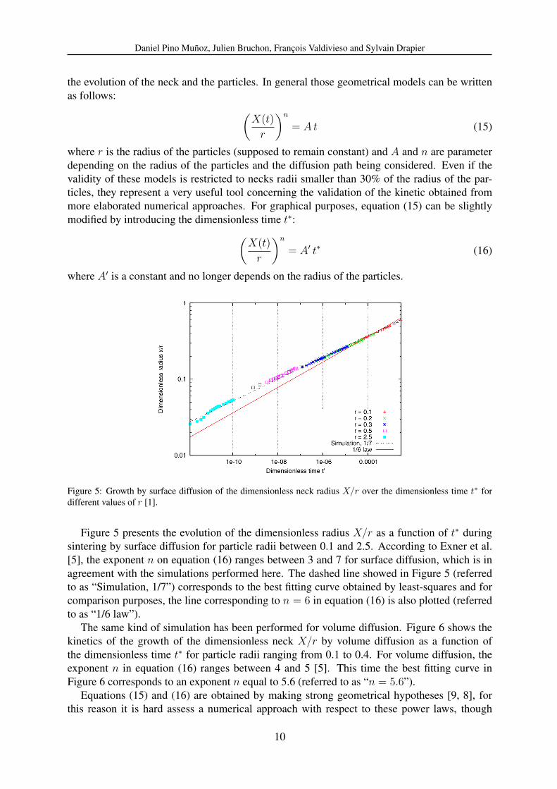
The same kind of simulation has been performed for volume diffusion. Figure 6 shows thekinetics of the growth of the dimensionless neck X/r by volume diffusion as a function ofthe dimensionless time t∗ for particle radii ranging from 0.1 to 0.4. For volume diffusion, theexponent n in equation (16) ranges between 4 and 5 [5]. This time the best fitting curve inFigure 6 corresponds to an exponent n equal to 5.6 (referred to as “n = 5.6”).

Equations (15) and (16) are obtained by making strong geometrical hypotheses [9, 8], forthis reason it is hard assess a numerical approach with respect to these power laws, though

10


those laws are very useful to analyze the kinetics of a specific diffusion path in a qualitativeway. Considering this, it is fairly safe to say that our approach is able to group the main mecha-nisms controlling both surface and volume diffusions, and is especially robust although pressurediscontinuities are to be computed numerically and volume has to be conserved. Nevertheless,a better understanding of the volume diffusion requires a deeper study of this diffusion path andthis study is yet to be done.

Figure 6: Growth by volume diffusion of the dimensionless neck radius x/r over the dimensionless time t∗ fordifferent values of r [2].

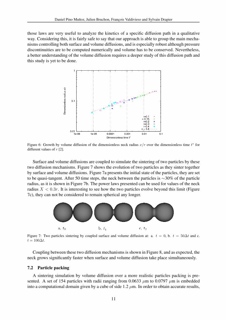
Surface and volume diffusions are coupled to simulate the sintering of two particles by thesetwo diffusion mechanisms. Figure 7 shows the evolution of two particles as they sinter togetherby surface and volume diffusions. Figure 7a presents the initial state of the particles, they are setto be quasi-tangent. After 50 time steps, the neck between the particles is ∼30% of the particleradius, as it is shown in Figure 7b. The power laws presented can be used for values of the neckradius X < 0.3r. It is interesting to see how the two particles evolve beyond this limit (Figure7c), they can not be considered to remain spherical any longer.

Figure 7: Two particles sintering by coupled surface and volume diffusion at: a. t = 0, b. t = 50∆t and c.t = 100∆t.

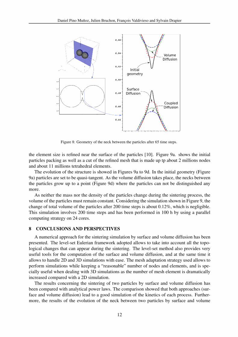
Coupling between these two diffusion mechanisms is shown in Figure 8, and as expected, theneck grows significantly faster when surface and volume diffusion take place simultaneously.

7.2 Particle packing

A sintering simulation by volume diffusion over a more realistic particles packing is pre-sented. A set of 154 particles with radii ranging from 0.0633 µm to 0.0797 µm is embeddedinto a computational domain given by a cube of side 1.2 µm. In order to obtain accurate results,

11


Figure 8: Geometry of the neck between the particles after 65 time steps.

the element size is refined near the surface of the particles [10]. Figure 9a. shows the initialparticles packing as well as a cut of the refined mesh that is made up tp about 2 millions nodesand about 11 millions tetrahedral elements.

The evolution of the structure is showed in Figures 9a to 9d. In the initial geometry (Figure9a) particles are set to be quasi-tangent. As the volume diffusion takes place, the necks betweenthe particles grow up to a point (Figure 9d) where the particles can not be distinguished anymore.

As neither the mass nor the density of the particles change during the sintering process, thevolume of the particles must remain constant. Considering the simulation shown in Figure 9, thechange of total volume of the particles after 200 time steps is about 0.12%, which is negligible.This simulation involves 200 time steps and has been performed in 100 h by using a parallelcomputing strategy on 24 cores.

8 CONCLUSIONS AND PERSPECTIVES

A numerical approach for the sintering simulation by surface and volume diffusion has beenpresented. The level-set Eulerian framework adopted allows to take into account all the topo-logical changes that can appear during the sintering. The level-set method also provides veryuseful tools for the computation of the surface and volume diffusion, and at the same time itallows to handle 2D and 3D simulations with ease. The mesh adaptation strategy used allows toperform simulations while keeping a “reasonable” number of nodes and elements, and is spe-cially useful when dealing with 3D simulations as the number of mesh element is dramaticallyincreased compared with a 2D simulation.

The results concerning the sintering of two particles by surface and volume diffusion hasbeen compared with analytical power laws. The comparison showed that both approaches (sur-face and volume diffusion) lead to a good simulation of the kinetics of each process. Further-more, the results of the evolution of the neck between two particles by surface and volume

12


Figure 9: Evolution of a particle packing through the time.

diffusions are in agreement with the predictions obtained from power laws. The simulation ofsintering by coupled surface and volume diffusions has been presented. Even if the results ofthis coupling seem to be in agreement with the kinetics of the process, it is very difficult tovalidate the results as there is no experimental data available for these two routes. Finally thecapabilities of the numerical approach has been demonstrated by performing a simulation of thesintering of more realistic 3D particle packing.

A large amount of work is yet to be done, mainly concerning the grain boundary diffusion.But the bases for the treatment of the diffusion path has been presented as the approach devel-oped to solve the mechanics can also be used to take into account the surface tension at the grainboundary. The mechanical problem has been solved by considering the particles to respond aslinear elastic isotropic materials, it would be very interesting to study how differently the struc-ture would evolve if another material model would be considered or if the mechanical propertiesof each particle were different. The global goal of this work is to simulate the sintering processof fully 3D granular packing, which would open huge perspectives regarding the computationalmaterials design.

REFERENCES

[1] J. Bruchon, S. Drapier, and F. Valdivieso. 3D finite element simulation of the matter flowby surface diffusion using a level set method. Int J Numer Meth Eng, 86(7):845–861,2011.

13


[2] J. Bruchon, D. Pino Munoz, F. Valdivieso, and S. Drapier. Finite element simulation ofmass transport during sintering of a granular packing. Part I. surface and lattice diffusion.J Am Ceram Soc, pages 1–8, 2012.

[3] T. Coupez. Reinitialisation convective et locale des fonctions level set pour le mouvementde surfaces et dinterfaces. Journees Activites Universitaires de Mecanique-La Rochelle,31 aout et 1er septembre 2006, 2006.

[4] H. Digonnet, L. Silva, and T. Coupez. Cimlib: a fully parallel application for numericalsimulations based on components assembly. In AIP Conference Proceedings, volume 908,page 269, 2007.

[5] H. E. Exner, E. Arzt, Robert W. Cahn, and P. Haasen. Sintering processes. In PhysicalMetallurgy (Fourth Edition), pages 2627–2662. North-Holland, Oxford, 1996.

[6] R. Fedkiw and S. Osher. Level-set methods: An overview and some recent results. JComput Phys, 169(2):463–502, 2001.

[7] K. Garikipati, L. Bassman, and M. Deal. A lattice-based micromechanical continuumformulation for stress-driven mass transport in polycrystalline solids. Journal of the Me-chanics and Physics of Solids, 49(6):1209–1237, 2001.

[8] C. Herring. Surface tension as a motivation for sintering. The physics of powder metal-lurgy, 27(2):143–179, 1951.

[9] G. C. Kuczynski. Self-diffusion in sintering of metallic particles. Transactions of theAIME, 185:169–178, 1949.

[10] Y. Mesri, W. Zerguine, H. Digonnet, L. Silva, and T. Coupez. Dynamic parallel adaptionfor three dimensional unstructured meshes: Application to interface tracking. Proceedingsof the 17th International Meshing Roundtable, pages 195–212, 2008.

[11] D. Peng, B. Merriman, S. Osher, H. Zhao, and M. Kang. A PDE-based fast local level setmethod. J Comput Phys, 155(2):410–438, 1999.

[12] D. Pino Munoz, J. Bruchon, S. Drapier, and F. Valdivieso. A finite element-based level-setmethod for fluid - elastic solid interaction with surface tension. Int J Numer Meth Eng, Toappear, 2011.

[13] M. Sussman, P. Smereka, and S. Osher. A level set approach for computing solutions toincompressible Two-Phase flow. J Comput Phys, 14(1):146–159, 1994.

[14] F. Wakai and KA Brakke. Mechanics of sintering for coupled grain boundary and surfacediffusion. Acta materialia, 59(14):5379–5387, 2011.

[15] Y.U. Wang. Computer modeling and simulation of solid-state sintering: A phase fieldapproach. Acta materialia, 54(4):953–961, 2006.

14

SOLID-STATE SINTERING SIMULATION: …bruchon/conferences/PinoMunoz_ECCOMAS2012.pdfSOLID-STATE...

Documents

Transcript of SOLID-STATE SINTERING SIMULATION: …bruchon/conferences/PinoMunoz_ECCOMAS2012.pdfSOLID-STATE...