SOLERGY A Computer Code Calculating the Annual Energy from ...
153
SANDIA REPORT SAN D86-8060 0 UC-62a Unlimited Release * Printed May 1987 SOLERGY - A Computer Code for Calculating the Annual Energy from Central Receiver Power Plants M. C. Stoddard, S. E. Faas, C. J. Chiang, J. A. Dirks Prepared by Sandia National Laboratories Albuquerque. New Mexico 87185 and Livermore. Calitornia 94550 for the United States Department of Energy under Contracl DE-ACO4-76DPOO78B
Transcript of SOLERGY A Computer Code Calculating the Annual Energy from ...

SANDIA REPORT SAN D86-8060 0 UC-62a Unlimited Release
* Printed May 1987
SOLERGY - A Computer Code for Calculating the Annual Energy from Central Receiver Power Plants
M. C. Stoddard, S. E. Faas, C. J. Chiang, J. A. Dirks
Prepared by Sandia National Laboratories Albuquerque. New Mexico 87185 and Livermore. Calitornia 94550 for the United States Department of Energy under Contracl DE-ACO4-76DPOO78B

.
Issued by Sandia National Laboratories, operated for the United States De artment of Energy by Sandla Corporation. N6TICE This report was prepared as an account of work sponsored by an agency of the United States Government. Neither the United States Government nor any agency thereof, nor any of their employees, nor any of the contractors, subcontractors, or their employees, makes any war- ranty, express or implied, or assumes any legal liability or responsibility for the accuracy, completeness, or usefulness of any information, apparatus, product, or process disclosed, or represents that its use would not infringe privately owned rights. Reference herein to any specific commercial product, process, or service by trade name, trademark, manufacturer, or otherwise, does not necessarily constitute or imply its endorsement, recommendation, or favoring by the United States Government, any agency thereof or any of their contractors or subconractors. The views and opinions expressed herein do not necessarily state or reflect those of the United States Government, any agency thereof or any of their contractors or subcontractors.
Printed in the United States of America Available from
National Technical Information Service 5285 Port Royal Road Springfield, VA 22161
NTlS price codes Printed copy: A08 Microfiche copy: A01
I

UC-62a SAND 86-8060 Unlimited Release Printed May 1987
SOLERGY - A Computer Code for Calculating the Annual Energy from Central Receiver Power Plants
M. C. Stoddard Sandia National Laboratories
Livermore, CA 94550
S. E. Faas Sandia National Laboratories
Livermore, CA 94550
C. J. Chiang Sandia National Laboratories
Albuquerque, NM 87185
J. A. Dirks Pacific Northwest Laboratories
Richland, WA 99352
ABSTRACT
The program SOLERGY was designed to simulate the operation and power output, of a user-defined solar central receiver power plant for a time period of up to one year. SOLERGY utilizes recorded or simulated weather data and plant com- ponent performance models to calculate the power flowing through each part of the solar plant. A plant control subroutine monitors these powers and determines when to operate the various plant subsyst,ems. Parasitic electrical power is computed on a 24-hour basis.


SOLAR THERMAL TECHNOLOGY
FOREWORD
The research and development described in this document was conducted within the U.S. De- partment of Energy’s (DOE) Solar Thermal Technology Program. The goal of the Solar Thermal Technology Program is to advance the engineering and scientific understanding of solar thermal technology, and t o establish the technology base from which private industry can develop solar thermal power production options for introduction into the competitive energy market.
Solar thermal technology concentrates solar radiation by means of tracking mirrors or lenses onto a receiver where the solar energy is absorbed as heat and convert.ed into electricity or incor- porated into products as process heat. The two primary solar thermal technologies, central re- ceivers and distributed receivers, employ various point and line-focus optics t o concentrate sun- light. Current central receiver systems use fields of heliostats (two-axis tracking mirrors) to focus the sun’s radiant energy onto a single tower-mounted receiver. Parabolic dishes up t o 17 meters in diameter track the sun in two axes and use mirrors or Fresnel lenses to focus radiant energy onto a receiver. Troughs and bowls are line-focus tracking reflectors that concentrate sunlight onto receiver tubes along their focal lines. Concentrating collector modules can be used alone or in a multi-module syst,em. The concentrated radiant energy absorbed by the solar thermal receiver is transported t o the conversion process by a circulating working fluid. Receiver temperatures range from 100°C in low-temperature troughs t o over 150OOC in dish and central receiver systems.
The Solar Thermal Technology Program is directing efforts t o advance and improve promising system concepts through the research and development of solar thermal materials, components, and subsystems, and the testing and performance evaluation of subsystems and systems. These efforts are carried out through the technical direction of D O E and its network of national labo- ratories who work with private industry. Together they have established a comprehensive, goal directed program t o improve performance and provide technically proven options for eventual in- corporation into the Nation’s energy supply.
To be successful in contributing to an adequate national energy supply a t reasonable cost, solar thermal energy must eventually be economically competitive with a variety of other energy sources. Components and system-level performance targets have been developed as quantitative program goals. The performance targets are used in planning research and development activi- ties, measuring progress, assessing alternative technology options, and making optimal component developments. These targets will be pursued vigorously to insure a successful program.
iii/iv


CONTENTS
1.0 Introduction 2.0 Major Component Models
2.1 Collector Field Model 2.2 Receiver and Piping Models 2.3 Thermal Storage Model 2.4(a) Turbine Operational Controller
2.4(b) Alternate Turbine Operational Controller Simple Dispatch
Value Maximizing Dispatch 2.5 Turbine Model 2.6 Parasitics Model
3.0 SOLERGY Input 3.1 SOLERGY Namelist Input: SOLNML.DAT 1
3.2 SOLERGY Input Weather Data: SOLM’EA.DAT 4.0 SOLERGY Output
4.1 Annual Energy Summary 4.2 Annual Efficiency Calculations
Appendix A-SOLER GY Subroutine Description Appendix B --Sample SOLERGY Problems Appendix C-The VALCALC Program Appendix D--Sample VALCALC Problems -4ppendix E-Thermal Storage Tank Heat Loss Factors References
Page 1 5 5 7
13 17
23
31 35 37 37 53 55 55 59 61 83
109 119 131 135

ILLUSTRATIONS
No.
1 SOLERGY Program Flow Diagram
2 Flowchart of Decisions for Subroutine RCVR
3 Thermal Storage Variable Definitions
4 Storage Energy Levels for Simple Dispatch
5 Phases of Turbine Startup
6 Levelized SCE Value Rates: Summer
7 Levelized SCE Value Rates: Winter
Page
4
8
14
18
20
24
25

TABLES
No.
I. NMLGEN Namelist Variables
11. KMLLOC Namelist Variables
111. NMLCOEF and NMLCOLF Namelist Variables
IV. NMLRCVR Namelist Variables
V. NMLPIPE Namelist Variables
VI. NMLSTRG Namelist Variables
VII. NMLTRBN Namelist Variables
VIII. DISPATCH Namelist Variables
IX. PRNTOUT Namelist Variables
Page
37
38
39
4 1
4 1
42
47
49
50


1.0 INTRODUCTION
The program SOLERGY was designed to simulate the operation and power output of a user-defined solar central receiver power plant for a time period of up to one year. SOLERGY utilizes recorded or simulated weather data and plant component models to calculate the power flowing through each part of the solar plant. A plant control subroutine monitors these powers and determines when to operate the various plant subsystems. There are two different plant control sub- routines available in SOLERGY-output maximizing and value maximizing. The user selects one of them to control plant operation for the entire simulation run. Parasitic electrical power is computed on a 24-hour basis. SOLERGY was devel- oped on a VAX 111780 with a VMS 4.0 operating system using the FORTRAN language.
SOLERGY is based on a solar central receiver annual energy simulation code called STEAEdl) . STEAEC was written to compare plant design proposals for the construction and testing of a pilot plant. This pilot plant, Solar One, was eventually constructed and tested. The annual energy based on STEAEC cal- culations was found to be noticeably different than that actually produced. This spurred an investigation of STEAEC, which uncovered several shortcomings. The most significant shortcoming was the failure to account for parasitic electrical power consumption over the entire day. STEAEC accounted for electrical para- sitic power only during during the daylight hours while the plant was operating. This was typical for annual energy estimation codes of the mid-seventies applied to solar central receivers.
More recently. a computer code providing estimates of annual energy output was needed for evaluating conceptual designs during a comprehensive study which ultimately provided technical data for a solar central receiver design handbook(2). A valuable tool motivated by the needs of this study, is a subroutine which con- trolled the simulated plant in such a manner that electricity was produced during hours of peak demand. This subroutine contains a thermal energy dispatch strat- egy that maximizes the plant revenue and profit. SOLERGY, when used with an ancilliary program called VALCALC, computes plant revenue over the simulation period. VALCALC calculates the value of electricity based on the avoided costs of the Southern California Edison Company as described in Appendix C.
As a result of the need for a more realistic prediction capability, STEAEC was rewritten, improving and expanding its capabilities, and renamed SOLERGY. The main features of SOLERGY are that it:
Utilizes actual or simulated site weather data a t time intervals as short as 7.5 minutes.
1

Computes net electrical energy output including parasitics based on a 24-hour day.
Incorporates advanced plant energy dispatching capability to better simulate plant usage in a utility grid.
Models single phase fluids (e.g. molten salt and liquid sodium). Water/steam systems can also be modelled with some effort.
Supports a sodium receiver passing heat to a molten salt storage system through an intermediate heat exchanger.
Requires no subroutines from commercial math software packages.
Receiver model has up-to-date thermal loss and startup time algorithms.
Storage model supports startup delays and allows the energy in storage to fall below zero (fluid colder than design minimum).
Turbine model supports delays for turbine roll, generator synchronization, and ramp to full load. Off-design point operation of the turbine can also be modelled.
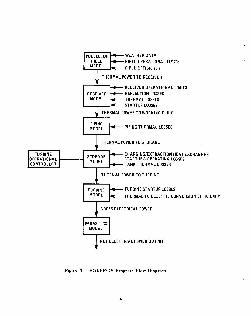
The basic program flow for SOLERGY is shown in Figure 1. For each time step, the collector field model concentrates the incident solar radiation and di- rects it onto the receiver. Logic within the receiver model decides whether the energy collection portion of the plant will operate based on the level of power de- livered by the collector field. All power from the receiver is delivered to thermal storage, provided that thermal storage can accept it, (i.e. storage is not full). The electricity production portion of the plant can be operated nearly independently from the energy collection portion, depending on which turbine operational con- troller is selected. Three levels of complexity are available within two plant con- trol subroutines for turbine operational control: sunfollowing (turbine operation is attempted whenever the receiver is operating), simple delay (turbine operation is delayed unt,il a specified energy level in thermal storage is achieved), and value maximizing (electrical power is produced during periods when its value is great- est. The parasitic model calculates electrical parasitics based on which portions of the plant are operational.
Power flow calculations are made for each time step, which can be chosen to be as small as 0.125 hour. Plant operational decisions are based on ambient weather, power incident on the receiver, thermal storage energy level, and time of day/year. The criteria for formulating these decisions will be more fully dis- cussed in the next section which describes the major plant component models. Following the component model descriptions are two sections, one describing the SOLERGY input and the other describing t,he output. Appendices A through D list all SOLERGY subroutines; sample problem input and output; a description of the program VALCALC, which calculates the value of electricity generated by
2

the plant and revenue from the plant; and a sample problem utilizing VALCALC. Appendix E contains additional details on thermal storage tank loss factors.
3
WEATHER DATA FIELO OPERATIONAL LIMITS
TURBINE MODEL
1 - L FIELO EFFICIENCY
- TURBINE STARTUP LOSSES - THERMAL TO ELECTRIC CONVERSION EFFICIENCY
THERMAL POWER TO RECEIVER
R ECEl V E R 0 PE RAT1 ON A L LIMITS RECEIVER REFLECT1 ON LOSSES
MODEL THERMAL LOSSES STARTUP LOSSES
THERMAL POWER TO WORKING FLUID
PIPING THERMAL LOSSES PIPING MODEL
PARASITICS MODEL
NET ELECTRICAL POWER OUTPUT 4 Figure 1. SOLERGY Program Flow Diagram
4

2.0 MAJOR COMPONENT MODELS
The main program of SOLERGY initializes the namelist variables (described in Section 3.1) and calculates design point efficiencies. A series of subroutines, corresponding to the major plant components shown in Figure 1, are then called sequentially for each time step. The main program tabulates daily and annual energy totals and writes them to output files.
2.1 Collector Field Model
Subroutine COLF
The collector field model directs the solar radiation incident on the heliostats onto the receiver. The collector field operates whenever the solar elevation an- gle and the ambient wind speed and temperature are within specified limits and if there is solar insolation. All of the collector field operational limits are user- specified and are discussed more fully in Section 3, the collector field namelist in- put description. The power to the receiver is calculated as:
PTR(K) = F * DNI(K) * FS * (1)
where:
F = collector field efficiency, DNI(K) FS PTR(K) K = current time step.
= incident solar radiation at time K, kW/m2 , = collector field reflective area, m2 , = power incident on receiver, MWt, and
The collector field efficiency accounts for losses due to heliostat reflectivity, cosine, shadowing, blocking, spillage, and wind speed. It is calculated as a func- tion of solar azimuth and elevation angles in the subroutine EFFIC.
Subroutine EFFIC
A two-dimensional collector field efficiency matrix is specified as input in the namelist NMLCOEF. This matrix is often referred to as an "az-el" table, since it gives the collector field efficiency as a function of solar azimuth and elevation angles. This field efficiency mat.rix can be generated by various computer codes,
5

such as DELSOL (3) or MIRVAL (4), and is discussed further in the namelist NMLCOEF section. The collector field efficiency matrix contains the effects of cosine, shadowing, blocking, and spillage. It may also contain the effect of he- liostat reflectivity. If the field efficiency matrix does not contain heliostat reflec- tivity, this factor can be accounted for in the collector field efficiency expression given by Equation 2. Field efficiency matrices generated by DELSOL also contain the receiver absorptivity. This factor was removed from the field efficiency ma- trix by dividing the DELSOL resultant by the receiver absorptivity. The receiver absorptivity is considered a part of the receiver subsystem; therefore, its effect is introduced in the receiver model. The decline in collector field performance with wind speed can also be included in the model. The collector field efficiency, F in Equation (l), is calculated at each time step as:
F = EFF * RFLCTY * EFWS(WS) (2)
where:
EFF
RFLCTY
EF W S ( W S)
= collector field efficiency from the
= heliostat reflectivity - if not included
= collector field efficiency as a function of
az-el table,
in EFF, and
wind speed, if known.
SOLERGY utilizes the subroutine TSPLIN, which interpolates the two- dimensional field efficiency matrix. The cubic spline routines SPLIFT and SPLINT efficiency factors.
are used for interpolation of the one-dimensional array of wind speed
6

2.2 Receiver and Piping Models
Subroutine RCVR
The receiver model in SOLERGY determines receiver operatam based on the current power aLYailable from the heliostat field and the previous receiver status. In addition to shutdown, startup, and rated operation modes, a derated operation mode is included. A limited time holding mode is available for a receiver with doors, permitting instantaneous restart after a period of low insolation.
The first section of the subroutine RCVR determines if the power to the re- ceiver is within its operational range. If the power to the receiver is greater than the receiver thermal rating, the input is decreased to the thermal rating, simulat- ing heliostat defocusing. If the power is less than the minimum, the power input is set to zero and the receiver shuts down (or remains shut down) or the receiver goes on hold if it has doors. In reality, the lower receiver power limit is set by the minimum flowrate that the receiver flow valves can handle. Figure 2 shows a flowchart representation of this decision-making process for the receiver.
The mode of receiver operation in the previous time step is examined next in the subroutine. Based on the receiver status and the thermal power available to the receiver (which was just calculated), a decision is made for the receiver to remain in its current operational mode or to transition to a new mode. If the re- ceiver is operating, the reflective and thermal power losses are calculated. The result is PTWF, the power transmitted to the working fluid.
Steady- St at e Rated Operation
The receiver remains in rated operation or transitions to rated operation when net positive power can be collected. The power to the receiver from the he- liostat field is represented by PTR(K), where K is the current time step. This quantity accounts for the collector field efficiency and heliostat reflectivity. The power which can be transferred to the working fluid is:
PTWF = EPS * PTR(K) - XLR(\VS(K))
where:
PTWF
EPS = receiver absorptivity PTR(K)
= thermal power delivered to the working fluid, MWt
= thermal power delivered by the heliostat field to the receiver, MWt, and
7
(3)

RECEIVER
DEFOCUS HEL1oSTATS so
POWER TO RECEIVER EQUALS
MAXIMUM ALLOWABLE
IS POWER TO THE No RECEIVER LESS THAN
f-- RECEIVER MAXIMUM POWER LIMIT?
+ SHUTDOWN Is NET To No DOES THE RECEIVER No
RECEIVER" GREATER THAN RECEIVER
HAVE DOORS?
1
HASTHE RECEIVER NO BEEN ON HOLD FOR + ON YES
HOLD 3 TIME STEPS? CONTINUE OPERATIONS I
OR BEGIN OPERATION IF
PREVIOUSLY SHUT DOWN SHUT DOWN
YES
*REDUCED BY REFLECTIVE, RADIATIVE, AND CONVECTIVE LOSSES
Figure 2. Flowchart of Decisions for the Receiver Subroutine
8

XLR(WS(K)) = receiver thermal loss due to convection and radiation as a function of wind speed, MWt.
A rough determination is then made of whether this power to the working fluid, PTWF, will result in net positive power collected by the receiver. This is done by estimating the thermal equivalent of the parasitics required to operate the solar portion of the plant, represented by the variable AUXCOST.
SPPAR = 0.0691 * (GPOWER)'.0408
and
AUXCOST = SPPAR/EPSS(74., 1.)
where:
SPPAR GPOWER AUXCOST
EPSS( 74.,1.)
= solar plant parasitics, MW, = gross power rating of the plant, MW, = thermal power equivalent of parasitic
power, MWt = thermal to electric conversion efficiency
for the turbine at nominal conditions.
(4)
( 5 )
The algorithm for calculating SPPAR is described in Section 2.6 which describes the parasitic model. The conversion of parasitic electrical power to its thermal equivalent utilizes the turbine conversion efficiency. The AUXCOST calcula- tion provides only a rough indication of net positive receiver power. If PTWF is greater than AUXCOST, the receiver is said to be generating net positive power.
Steady- St at e De rat ed Ope ration
The receiver enters a derated operational mode when the power it collects is less t,han AUXCOST, but still greater than the minimum power limit of the receiver. This is expressed as:
AUXCOST > PTWF > RMF * RS
where:
RMF RS
= receiver minimum flow fraction, and = receiver thermal rating, MWt.
9

Derated operation is permitted for three consecutive time steps, after which time a receiver without doors shuts down and a receiver with doors goes into the hold mode.
Receiver Hold Mode
The hold mode simulates the operation of a receiver with doors. During peri- ods of low insolation the doors are closed and the heat transfer fluid is circulated through the receiver in anticipation of a receiver restart. This mode of operation is permitted for three time steps. If the insolation returns to an acceptable level, receiver operation commences with no startup delay. If, after three time steps in the hold mode, the insolation is still too low for receiver operation, the receiver is shut down. A receiver with doors shuts down immediately (no hold mode) if the low insolation occurs within three time steps of sunset. If it is of interest to change the number of time steps associated with the receiver door simulation, this change must be made in the RCVR subroutine (this is not an input variable).
Receiver Shutdown
R.eceiver shutdown can occur as the result of low insolation or sunset. Either of these conditions results in zero power being delivered to the working fluid.
Receiver Startup
Receiver startup is initiated when the power which would be delivered to the working fluid if the receiver w&s operating exceeds the minimum allowable power delivered to the working fluid. That is:
EPS * PTR(K) - XLR(WS(K)) > (RMF * RS)
The transient receiver startup requirements are based on when the receiver was last shut down. The fraction, XTO, between zero and one, represents the cur- rent state of the receiver. A value of zero indicates that the receiver is cold, and a value close to one indicat.es that the receiver is warm. The value of XTO is in- fluenced by both the length of time that the receiver has been shut, down and the receiver cool down parameter.
(-TRSHUT t ALPHAR) XTO = e
where:
(7)
XTO = current receiver state (0 <_ XTO 5 l ) , TRSHUT = time the receiver has been shut down, hours, ALPHAR = receiver cool down parameter (hrs-I).
10

User input to the receiver namelist allows the specification of a time and/or energy required for receiver startup from a cold state. These variables are TREQD and EREQD, respectively, and are described in more detail in Section 3. The receiver state. XTO, causes these variables to be scaled, establishing the current init,ial state of the time (TINIT) and/or energy requirements (EINIT) for startup.
TINIT = TREQD * XTO
EINIT = EREQD * XTO
The time and energy required to start the receiver are then calculated as:
TTOSTART = TREQD - TINIT
ETOSTART = EREQD - EINIT
Once both of these requirements are satisfied, the receiver transitions to ei- ther rated or derated operation. During startup, although power is directed onto the receiver: no power is delivered to the working fluid. This energy loss due to receiver startup is collected in the variable RCVRSTRT, which is reported sepa- rately in the output as a receiver startup energy loss.
Subroutine PIPE
The PIPE subroutine calculates thermal losses in the piping as a function of ambient dry bulb temperature, DBT. The power loss in the piping is calculated as:
PWF = PTWF - RS * XLP(DBT) (12)
XLP(DBT) is the power loss in the piping, expressed as a fraction of the receiver thermal rating. This is a user input variable. The power to the working fluid from the receiver, PTWF, is decreased by the piping loss, resulting in power in the working fluid, PWF.


2.3 Thermal Storage Model
Subroutine STRG
All power from the receiver is sent to thermal storage. Power used to oper- ate the turbine for electrical power generation is extracted from thermal storage. Thus, the storage subroutine in SOLERGY responds to the demands placed on it, by the receiver subroutine and turbine controller subroutine. SOLERGY is a power flow model; however, thermal storage must be energy based. Power multi- plied by the time step gives the energy added to or extracted from thermal stor- age. Thermal storage is limited by the thermal rating of its charging and extrac- tion heat exchangers, if present, and by its state of charge. As is true for all of SOLERGY, the various thermal power gains and losses are handled in a quasi- steady manner by assuming that all powers are constant during a time interval. The storage subroutine also supports rudimentary transient response through the mechanism of a time and/or energy delay before useful operation can commence (Le. startup delay). Useful operation is defined as transferring energy into storage or delivering steam to the turbine. Charging and extraction of thermal storage can occur simultaneously.
Normal Operation
Three basic equations (13-15) are used in calculating the energy exchanges in thermal storage: the equation for normal operation, a transient charging startup condit,ion, and a transient extraction startup condition. The equation for normal operation is as follows:
ENEW = ES + [(PTS - TPLDC) - (TPLFT + TPLBTC)
-(PFS + TPLDD)] * DELT
where:
ES ENEW PTS
TPLDC
TPLFT
TPLBTC
= previous amount of energy in storage, MWthr, = updated amount of energy in storage, MWthr, = thermal power delivered to storage by the receiver via
= thermal power lost to the environment in the charging
= the thermal power lost by the storage tank to the
= the thermal power lost through the exchange of heat
the piping system, MWt.
heat exchangers and charging piping, MWt.
environment, MWt.
13

across the thermocline between the hot and cold regions, MWt. This is for thermocline tanks only.
= the thermal power delivered to the turbine or process, MWt. = the thermal power lost to the environment by the
= the time interval, hours.
PFS TPLDD
DELT extraction heat exchangers and piping, MWt.
Figure 3 associates these variables with particular components of thermal storage.
TPLBTC TPLFT
TPLDC
PFS 2 = PFS + TPLDD
STORAGE TANK(S) PTS
E XT R ACT1 0 N CHARGING
PTS 2 = PTS - TPLDC
TPLDD
Figure 3. Thermal storage variable definitions
There are maximum and minimum limits on the thermal storage charge and extraction rates. If the maximum limit is exceeded, the excess is calculated and reported in the variable SUPTS for charging and UPFS for extraction. The value of SUPTS and UPFS is used to signal the subroutine HANDLER (described in the next section) that a mismatch of power flows has occurred and must be cor- rected. If the power level (PM’F or PFS) falls below the minimum rate for the charging or extraction loop, that loop will be shut down. If the power level is be- low the minimumand non-zero, the value of SUPTS or UPFS will be set equal to the power level, signalling HANDLER that the power cannot be absorbed by storage or delivered to the turbine.
14

There are maximum and minimum limits on the amount of energy which can be contained in thermal storage. If the maximum stored energy is exceeded in a particular time interval according to Equation (13), a new charging power level that will just fill storage to its maximum is back-calculated. This new power level (PTS) is used to calculate the excess power, which is then stored in the variable SUPTS. If the new power level is below the minimum charge rate, the charging loop is halted. The difference between the request (PFS) and the available power is stored in the variable UPFS-unavailable power from storage. Likewise, if more power is requested for the turbine (PFS) than is available from storage, then the. extraction request must be reformulated. If this new value is below the minimum, the extraction loop is halted. In either case, the value of SUPTS or UPFS is sent back to the subroutine HANDLER which then revises the power sent to storage or the power extracted from storage. Further details of thermal storage operation are presented in Appendix A.2.
Transient Ope ration
Since heat exchangers cannot be brought from standby to full power opera- tion instantaneously, the storage subroutine provides the user with two tools for modelling the lag associated with bringing a heat exchanger or pipe and valve network to rated operating conditions: a time lag and an energy lag.
Since some energy must be expended during startup, a startup power must be defined. The maximum startup power levels for the charging and extraction loops are specified by the variables PWARMC and PWARMD, respectively. The power flow during startup is limited to these values plus the appropriate thermal loss. That is, the charging power limit (PTSMAX) and the maximum rate of energy extraction from the storage dank during transition (PFS2) are:
PTSMAX(,,,,,i,,t) = PWARMC + TPLDC (14)
PFS2 = PWARMD + TPLDD (15)
The variable PFS2 is the thermal power extracted from the storage tank. No thermal energy is delivered to the turbine during extraction startup and no ther- mal energy is delivered to the thermal storage tank during charging startup. The storage subroutine will remain in the transition mode for charging or extraction until the time and energy delay requirements are met.
Subroutine HANDLER
The subroutine HANDLER is called only if an unsatisfied condition is de- tected in the storage subroutine. HAIL’DLER performs the necessary adjustments to resolve this condition, which can result from an unacceptable power to storage
15

from the receiver, an unacceptable request for power by the turbine, or an extrac- t ion/ turbine st artup condition.
The subroutine HANDLER is called if either of the following two conditions exist. The first condition is if either of the storage values SUPTS or UPFS is non- zero, that is, if the thermal storage system either cannot accept the power de- livered by the receiver subsystem (SUPTS # 0 ) or cannot supply the requested amount of power to the turbine (UPFS # 0). HANDLER calculates the required reductions in the appropriate power streams. If necessary, it back-calculates re- quired reductions in power to the receiver (PTR), simulating heliostat defocus- ing. Energy losses due to defocusing heliostats are reported in SOLERGY output (Section 4.2 contains further details).
The second condition which will result in a call to HANDLER is startup of the storage extraction and turbine subsystems. HANDLER must delay the tur- bine startup until the STRG subroutine has completed the extraction heat ex- changer warm up. Once the extraction heat exchanger is warm, energy can be sent through it to begin the turbine startup.
16

2.4(a) Turbine Operational Controller Simple Dispatch
Subroutine G ONOGO
The GONOGO subroutine provides the turbine operational strategy. It mon- itors the energy €eve1 in thermal storage. When a specified level is reached, the t.urbine startup is initiated. GONOGO brings the turbine to full power and con- tinues operation at full power until storage is exhausted.
The GONOGO subroutine is called from the main program after the subrou- tine PIPE. GONOGO can also be called from the subroutine HANDLER (Sec- tion 2.3) if: (i) storage cannot supply the power that GONOGO has requested for the turbine or (ii) HANDLER detects that the extraction heat exchanger has successfully completed startup and turbine startup should begin. GONOGO ex- amines a set of turbine operational flags and branches to various sections of the subroutine based on the turbine status during the last time step. The basic goal of GONOGO is to decide when to begin turbine startup. Once begun, it will continue to operate the turbine at rated conditions whenever possible until the energy in storage is depleted. GONOGO formulates the request for power from storage, PFS, for turbine startup and operation. The subroutine branches which correspond to the various turbine operational modes will now be described.
Turbine Previously Shutdown
GONOGO allows the user the basic capability to specify the level of storage charge at which turbine startup will be initiated. This is accomplished through the set of input variables ESMIN1, ESMAX1, ESMIN2, and ESMAX2. There is a simple construct in GONOGO for requesting that turbine startup is delayed until the on-peak period is reached. For Southern California Edison during the summer months (days 155 through 280 in 1984), the on-peak period begins at noon; for the winter months, this period begins at 1700 (Daylight Savings Time). Although on-peak periods do not occur on holidays or weekends, this fact is not recognized in the GONOGO dispatch strategy. Every day is treated the same way. Electrical power generated during the on-peak period has a greater value than power gen- erated during the off-peak or mid-peak periods. If i t is before the on-peak period then CSMAXl and ESMAX2 govern turbine startup. If it is during the on-peak period then ESMINl and ESMIN2 govern turbine startup.
During the on-peak period, ESMINl and ESMIh’2 dictate the minimum stor- age charge level which must exist before the turbine can be started (Figure 4). ESMINl is used when the receiver is at rated operation and ESMIN2 is used when the receiver is not operating. In general, turbine startup can be initiated with less energy in storage if the receiver is operating since it is assumed that the
1 7

EMAX
ESMINZ: START TURBINE NOW IF RECEIVER IS NOT OPERATING
ESMINl: START TURBINE NOW IF RECEIVER IS OPERATING
EMIN
(a) On-peak Period
ESMAXZ: START TURBINE NOW IF RECEIVER IS NOT OPERATING
ESMAX1: START TURBINE NOW IF RECEIVER IS OPERATING (AVO IDS DISCAR D)
(b) Mid- or Off-peak Period
Figure 4. Storage Energy Levels for Simple Dispatch
18

receiver will continue to supply energy to storage. ESMINl should therefore be less than ESMIN2.
During the off-peak period, ESMAXl and ESMAX2 dictate the storage en- ergy levels a t which the turbine will be started. Similar to the previous situation, ESMAXl applies when the receiver is operating and ESMAX2 applies when it is not operating. Selection of a value for ESMAXl influences the amount of energy which will be discarded due to limited storage capacity. If the value chosen for ESMAXl is close to the maximum storage capacity, EMAX, when turbine startup is finally initiated, it may not be completed in time to avoid discard. However, if a low value is chosen for ESMAXl, turbine startup will be attempted whenever this minimal storage charge level exists. Specifying low values for ESMINl and ESMAXl provide the sunfollowing dispatch in which the turbine attempts to run whenever the receiver is collecting energy.
Clearly, for systems with smaller thermal storage capacities, there is less abil- ity to shift turbine operation to gain more revenue from power production with- out discarding unacceptably large amounts of energy. With smaller capacity ther- mal storage systems, it is recommended that minimal values of ESMINl and ESMAXl be selected in order to avoid energy discard when thermal storage is full. It is still important, however, to select large enough values of ESMIN2 and ESMAX2 to prevent GONOGO from attempting turbine startup when there is no chance of achieving successful power production.
With thermal storage systems of larger capacity, multiple runs of SOLERGY may be required in order to locate the optimal turbine operation for the system under consideration. The main variable to change between runs should be the value of ESMAX1.
Turbine Previously in Startup
Once the conditions for turbine startup are achieved, the turbine startup pro- cess begins. Figure 5 illustrates the phases of turbine startup. Since the thermal storage extraction heat exchanger must first be warmed before initiating the tur- bine startup, a two-layered turbine startup procedure is employed. First, the re- quest for minimum power from thermal storage is made:
PFS = TMFS * TPFSL (16)
The thermal power required by the turbine for rated operation is represented by TPFSL. TMFS is the fraction of TPFSL which sets the minimum level at which the turbine can operate. The thermal energy extracted from st,orage is used first in a prestart mode to warm the extraction heat exchanger. This energy is accu- mulated in the variable EXTRSTRT. No power is actually sent to the turbine.
When the prestart condition is successfully terminated (extraction heat. ex- changer is warm), then the actual turbine startup is initiated. The length of time
19
_- --__I__- __

TPFSL
W a a a 0 I- v)
0
U
w
0
I a
a 3 n
TMFS * TPFSL PWARMD
I I r 1 1-
t t W z - m a 3 I- O I- I- z W v)
I 4 G
a 0 I- s W z W a
t
0 W I- a a A -1 3 U
Figure 5 . Phases of turbine startup
that the turbine has been shutdown is examined. This value determines if the turbine startup will be hot, warm, or cold. -4 hot startup requires that the tur- bine was shut down less than TBHWS hours ago; a warm startup is used if shut- down was less than TBWCS hours ago, and a cold startup is used if shutdown was more than TBWCS hours ago. The default values for these input variables are 12 and 72 hours, respectively. They are described further in Section 3.0 under the namelist NMLTRBN input section.
The turbine shutdown time governs the selection of synchronization and ramp delays for the startup. The times of these delays are calculated for a cold startup as :
TSl = TIM(K) + SDC (17)
20

TS2 = TS1+ RDC (18)
where:
TS 1 TS2 TIM(K) SDC RDC
= time at which the synchronization will be completed, = time at which the ramp delay will be completed, = time of the day (hrs), = cold synchronization time delay (hrs), and = cold ramp time delay (hrs) .
TSI and TS2 are calculated for warm and hot conditions in a similar manner em- ploying the warm and hot synchronization delays, SDW and SDH, and the warm and hot ramp delays, RDW and RDH, respectively. These input variables are dis- cussed more fully in the turbine namelist description of Section 3.
A request is made for minimum power from storage, PFS1, as either the mini- mum storage extraction rate, PFSMIN, or TMFS * TPFSL, whichever is greater.
A second temporary request for power from storage, PFS2,, is formulated as:
PFS2 = PM/EPSS(WBT(K),PMX)
The ratio PMX is calculated as:
(19)
PMX = (TIM(K) - TSl)/(TS2 - TS1) (20)
If the current time is greater than TS1 (PMX > 0 ) , then the turbine ramps to its rat,ed power production according to:
PM = PMX * EPSS(WBT(K), 1) * TPFSL
where EPSS is the turbine thermal to electric conversion efficiency. The value of PFS2 (a local variable and different) from the local variable PFS2 in STRG) is zero if the synchronization time delay has not yet been satisfied. The final request for power from storage is chosen to be the greater of PFSl and PFS2.
When GONOGO is entered wit,h the turbine in startup and both the synchro- nization and ramp delays have been satisfied, the turbine transitions to rated op- eration.
Storage Unable to Satisfy Turbine Demand
This segment of the code occurs after the branches to other portions of the subroutine for turbine shutdown or startup have been made. Thus, it will be reached only by a call to GONOGO from HANDLER aft.er the thermal storage subroutine has signaled that it is unable to supply the requested power, PFS,
21

while the turbine is in rated or derated operation. This section of GONOGO ex- amines the new value of PFS formulated by HANDLER. If it is above the mim- imum threshold of turbine operation (TMFS * TPFSL), but less than the power required for rated turbine operation, GONOGO will place the turbine in derated operation. However, if the new value of PFS is less than (TMFS * TPFSL), then GONOGO shuts the turbine down, formulating a revised request of zero power from storage. It then returns control to HANDLER.
Turbine an Rated or Derated Operation
Regardless of whether the turbine was previously in rated or derated opera- tion, GONOGO always requests enough power for rated operation from storage:
PFS = TPFSL (22)
The storage subroutine must evaluate this request each time step to de- termine if it can satisfy this demand. If the request cannot be satisfied, then HANDLER is called and in turn calls GONOGO with a revised value of PFS. GONOGO determines if the new value of PFS is sufficient for continued turbine operat ion.
22

2.4(b) Alternate Turbine Operational Controller Value-Maximizing Dispatch
Subroutine MAXOUT
MAXOUT is a version of subroutine GONOGO that has been modified to maximize the value of electricity generated by a solar plant. This objective is accomplished by operating the turbine during the on-peak period of a utility in preference to the mid-peak and off-peak periods. Also, MAXOUT attempts to operate the turbine during the mid-peak period in preference to the off-peak pe- riod. The increase in value of electricity that can be obtained by using MAXOUT can be substantial and may be obtainable with little or no increase in cost. The net benefit of value-maximizing dispatch depends on the utility, the solar plant design, the insolation, and the amount of additional thermal storage that may be required to allow the solar plant to regularly supply electricity during the on-peak and mid-peak demand periods.
The value-maximizing thermal energy dispatch strategy used in MAXOUT is designed for the rate periods of the Southern California Edison Company (SCE). These rate periods are defined in SCE Schedule TOU-8 ( 6 ) . Figures 6 and 7 show the maximum value per unit of electric energy as a function of clock time, for a weekday during the summer and winter seasons, respectively. Weekends and holi- days are entirely off-peak periods. The value rates plotted in these figures are lev- elized over plant, lifetime and are normalized by the maximum value rate, which occurs during the on-peak period of the summer season. The value rate varies greatly during a day because of the high capital costs of peaking plants. Electric- ity generated by a solar plant may earn the maximum value rate only if the solar plant can be relied upon to deliver electricity during the on-peak period. Further explanation of the value of electricity can be found in Appendix C and in the de- tailed description of subroutine MAXOUT in Appendix A.2.
At the time of this writing, only SCE's rate structure has been examined. Appendix C.2 outlines modifications that would be necessary to use MAXOUT for utilities other than SCE. The dispatch strategy is a modified version of the dispatch strategy that was developed for the computer program SUNBURN ('1. The following is a description of the objectives of thermal energy dispatch for so- lar plants in general. Then, the dispatch strategy used in MAXOUT is briefly de- scribed. Finally, turbine operation is described for several hypot het(ica1 situations. Details of the algorithms used in MAXOUT can be found in Appendix A.2.
23

24

0
cv hi ....... .........
. . . . . . . . .
. . . . . . . .
. . . . . .
. . . . . .
. . . . . .
. . .
. . . . . .
. . . . . .
. . . . . . . . .
..,.......
J 1 : 1 :
1 : 1 :
I!
1 ; 1 :
: . . . . . . . . . . . . . . I ; . . . . . I.
: i ........................ . .
. . . . .
, . ._. .
.......... , .
..
.............
.............
. . . . .
. . .
. . . . . . . . .
........... .......... 0 ad 7
............
I I I I' . ' . . ' " ' . I I I I I
. . . . . . . . . . . . . . . . I . . . . . . . . . . . . . . . . . . .
. . . .
....
. . . .
. . .
0 ui 7
..................
0 f a , E
si=
.. . . . . . . . . . . . . . . . . . . . . . . . . . . . .
................................
1 . . . . . . . . . . . ; . . . . . . . . . . . . . . . . . I I I I I
.......................
. . . . . . .
. . . . . . . . .
. . . . . . . . . .
. . . . . . . .
. . . . . . . .
. .
. . . . . . . . . .
__ . ._ .. . . . . . . . . . . r !y
9 0 0 0
0 7
w u rn . . . . . . . . . . . ......... .............................. . . . . . . .
0 ,ad . . . . . . . . . . . . . . . . . . . 1 . . . . . . . .
. . . . . . . . . . . . ..................... 9 'co
. . . . . . . . . . . . . . . . . . . . . . . . .
. . . . . I I I I I
I
I 1 I I I I
.................. .......
0 . o
Z'l 0'1 Z'O 0
25

Objectives of Thermal Energy Dispatch
Thermal energy dispatch is simply defined as the manner in which thermal energy is used in a power plant. There are several possible objectives of thermal energy dispatch strategies for a solar plant. These are listed below:
1. to minimize discard of thermal energy-discard occurs when thermal storage is full and the receiver thermal power output exceeds the turbine energy con- sumption rate,
2. to maximize turbine efficiency-run the turbine at full power,
3. to maximize turbine life-minimize the number of turbine starts, and
4. to maximize value of electricity-operate the turbine during high demand pe- riods in preference to low demand periods.
The principal problem for thermal energy dispatch strategies for solar plants is the variation in insolation. The principal tool used to deal with this problem is thermal storage.
The Dispatch Strategy of MAXOUT
The thermal energy dispatch strategy in MAXOUT attempts to satisfy all four of the objectives listed above. Often, one objective can be satisfied only at the expense of anot,her. For example, to satisfy the fourth objective it is desirable to postpone turbine startup, allowing storage to be filled. However, to satisfy the first objective, it is desirable to advance turbine startup to avoid possible over- flow of storage. Therefore, tradeoffs must be made. The rules and assumptions that are used in MAXOUT to make these tradeoffs, which correspond to the four objectives described above, are as follows:
a. A prediction of energy flows is used to determine when to start. t,he turbine so that overflow of storage is avoided,
b. The prediction of energy flows is based on running the turbine at full power,
c. The turbine is run at less than full power, rather than shut down, if thermal energy must be conserved for use during the on-peak period, and
d. A prediction of energy flows is used to determine when to start the turbine so that the maximum amount of energy is stored prior to turbine startup, consis- tent with objective # 1 above. Before the on-peak period, the turbine may be derated if it is predicted tha.t insufficient energy will be available to operate the turbine at full power throughout the on-peak period. After the on-peak or mid-peak periods, and on weekends and holidays, the turbine may be shut down before storage is exhausted to allow for the possibility that there will be insufficient insolation to run the turbine during the on-peak and mid-peak periods for the next day or the day after the next day.
26

The dispatch strategy controls turbine startup, operation, and shutdown ac- cording to the following energy quantities:
PHBT: the predicted amount of thermal energy collected by the receiver from the current time until sunset,
ES: the amount of energy currently in storage, and
SCOI, SC02, and SC03: calculated values of thermal storage, called car- ryover storage.
PHBT is calculated by subroutine PREDICT. PREDICT uses one of two pre- dicted insolation arrays: SUNP(*) and SUNAP(*). SUNP(*) is updated once at the end of each day within the main program. SUNP(*) is derived exclusively from the actual insolation for previous days. SUIVAP(*) is set equal to SUNP(*) at the beginning of each day. Then, for each time step that the sun is above the horizon, subroutine ADJPRE adjusts SUNAP( *), for each time step until sunset, according to the difference between the predicted and the actual insolation value for the current time step. Details of the adjustment procedure may be found in the description of subroutine ADJPRE in Appendix A.l.
The dispatch strategy uses thermal storage:
to avoid discard of thermal energy when the receiver collects more power than the turbine can use, and
to insure generation of power during the on-peak period, even if there is no incident solar energy at this time.
The effectiveness of the dispatch strategy in accomplishing these goals depends on the solar multiple, storage capacity, and insolation. The carryover storage en- ergy levels, SCO1, SCO2, and SC03, are calculated and used to accomplish the second objective, without precluding the first. The carryover storage levels are calculated once at the beginning of each day from the variable SMAX, which is the maximum level of thermal energy in storage that is predicted to occur for the day, subject to the following two assumptions:
1. storage is empty at the beginning of the day, and
2. the turbine is started at time T, where
T = (time at the end of the on-peak period) - PHBT/TPFSL,
TPFSL is thermal energy consumption rate of the turbine at full power,
PHBT is the predicted amount of energy collected by the receiver from the current time until sunset, and
For weekends and holidays (off-peak periods), the start and the end times of the on-peak period are set to the time when sunset occurs.
27

SMAX is calculated at the beginning of each day using the insolation prediction SUNP(*). The calculation is performed by subroutine SCOVER (see Appendix A) according to the following procedure:
i ES(i) = (PTS(j) - PTT(j))dt, and
j = 1
SMAX = Max[ES(i)],
where:
ES(2’) = ith value of energy in storage, MWth,
PTS(j) = power to storage for j t h time step, MWt,
PTT(j) = power to turbine for j t h time step, MWt, and
dt = duration of time step, hours
The carryover storage levels are calculated as follows:
SCOl = (EMAX - SMAX), with SMAX calculated for today
SCOZ = (EMAX - SMAX), with SMAX calculated for tomorrow (the on- peak period may end at a different time tomorrow)
SC03 = SCOZ + (E - PHBT), where:
E is the greater of E’ and E”,
E’ is the energy required to run the turbine at, full power from the begin- ning of the mid-peak period today through the end of the on-peak period today, and
E“ is the energy required to run the turbine at full power from the be- ginning of the mid-peak period tomorrow through the end of the on-peak period tomorrow.
The carryover storage levels are constrained to be between zero and EMAX.
There are three major daily time intervals during which the turbine will be operated using a different procedure:
a.. before and during the on-peak period,
b. during the mid-peak period which occurs after the on-peak period (summer only, see Figures 6 and 7), and
28

c. during the off-peak period which occurs after the on-peak period, and during weekends and holidays.
SCOl is used to control turbine startup and operation during interval a; SC02 is used to control turbine operation during interval b; and SC03 is used to control turbine startup and operation during interval c.
The dispatch strategy attempts to reserve SCOl in thermal storage before the on-peak period. This is accomplished by delaying turbine startup and, if neces- sary, by derating the turbine before the on-peak period. Since SC02 is SCOl cal- culated for tomorrow (see above), during time interval b the turbine is shut down when the energy level in storage drops below SC02. Thus, the next day will begin with the next day’s value of SCOl in storage.
Time interval c is during the off-peak period. It is desirable to shift genera- tion of electricity from the off-peak period to either the on-peak or the mid-peak periods. Thus, in time interval c, if PHBT is less than SC03, the turbine will be shut, d0wn.t Details of the algorithms used in MAXOUT can be found in Ap- pendix A.2.
Ezamples of Turbine Operation
MAXOUT attempts to run the plant according to a certain plan. If variations in insolation cause deviations from this operational plan, then MAXOUT adjusts energy flows to drive the plant back towards this plan. This operational plan can be illustrated by describing plant operation on a baseline day. A baseline day oc- curs when the insolation prediction is correct, not only for the current day but for several preceding days. For a solar plant with a field sufficiently large to run the t,urbine during at least the on-peak period, a baseline day can be characterized by the following occurrences:
- The day begins with SCOl in storage,
- The turbine is started at time T, where T = [(end time of the on-peak pe- riod) - PHBT/TPFSL]
- Aft,er startup, the turbine is run at full power through the end of the on-peak period,
- During the day, the maximum thermal energy level in storage will be EMAX, the storage capacity, and
- The turbine will be shut down with at least SC02 in storage.
If less insolation occurs than was predicted, then the following may occur:
t MAXOUT assumes that loss of heat from thermal storage can be neglected for the purpose of value-maximizing dispatch.
29

(t) If the shortfall in insolation is detected before turbine startup, then turbine start will be delayed.
(ai) If the shortfall in insolation is detected after turbine startup, then the turbine will be derated, preserving SCOl in storage for possible use during the on- peak period. During the day, the maximum level of thermal energy in storage may be less than EMAX.
If more insolation occurs than was predicted, then the following may occur:
(i) If the excess of insolation is detected before turbine startup, then turbine start will be advanced.
(ai) If the excess of insolation is detected after turbine startup, then thermal en- ergy might be discarded. (Actually, the calculation of SMAX in subroutine SCOVER overestimates SMAX by a small amount, so that discard may not occur whenever actual insolation exceeds predicted insolation (see Appendix A).
30

2.5 Turbine Model
Subroutine TRBN
The subroutine TRBN uses the thermal power delivered from thermal storage to produce electricity. Since the steam generation system is modeled in the stor- age subroutine as the extraction heat exchanger, the turbine subroutine simply converts this thermal power into electrical power. The turbine is always in one of four modes: (2) shutdown, (ii) startup, (iii) rated operation, or (io) derated oper- ation.
The subroutine GONOGO, which acts as the system controller, determines the operational state of the turbine. If sufficient power can be sent to the turbine from thermal storage, the turbine operates. If sufficient power is not available from thermal storage, GONOGO shuts the turbine down.
As explained in the previous section, MAXOUT is an alternative system con- troller. Like GONOGO, MAXOUT determines the operational state of the tur- bine. However, the turbine operational state is determined using parameters other than just the amount of energy in storage. MAXOUT decides whether to start the turbine and whether to run it in a rated or derated mode based on (2)
the amount of energy in storage, (ii) a prediction of receiver output for the re- mainder of the day, (2;;) the present rate period of the day (on-peak, mid-peak, or off-peak), and (zu) the amount of time until the end of the on-peak period.
Turbine Shutdown
The turbine shutdown mode is straightforward. The subroutine GONOGO determines if there is sufficient power delivered from thermal storage for turbine operation. If sufficient power is not available, the turbine is shut down. Power to the turbine from storage (PTT) is set to zero, as is gross electrical power deliv- ered from the turbine (PFT = 0). The variable representing thermal power from storage, PFS, is always equal to PTT since direct tuibine operation from the re- ceiver was not intended to be an option in SOLERGY.
Turbine Startup
When turbine startup is initiated, synchronization and ramp delays are expe- rienced before operation commences. When the controller subroutine GONOGO starts the turbine, it calculates the times at which the synchronization delay and ramp delay will be completed. The magnitude of these delays is calculated in GONOGO. The delays depend on how long the turbine has been shut down.
31

There are provisions for a hot start, a warm start, and a cold start. Further de- tails of the synchronization and ramp delays were discussed in Section 2.4a.
Prior to completion of the synchronization time delay, all power sent to the turbine from thermal storage is used to warm the turbine. No electrical power is produced. All of the “lost” power is accumulated in the variable TRBNSTRT, which reports it as turbine startup energy in the output. Once synchronization has been completed, the electrical output of the turbine is gradually increased until the ramp time delay has been satisfied. If sufficient power continues to be available from thermal storage, the turbine transitions to rated or derated opera- tion.
Rated Turbine Operation
When thermal storage is able to supply sufficient power for rated turbine op- eration, the thermal to electric conversion efficiency is used to compute the gross electrical output from the turbine. The function EPSS provides the conversion ef- ficiency as a function of ambient wet bulb temperature and steam mass flow rate. When full power is supplied from thermal storage, the mass flow fraction is unity.
PFT = EPSS(WBT(K), 1.) * TPFSL
where:
PFT EPSS TPFSL
WBT(K)
= gross electrical power from the turbine, MWc, = turbine thermal to electric conversion efficiency, = thermal power required by the turbine for rated
= ambient wetbulb temperature, a F. operation, and
Derated Turbine Operation
The turbine is permitted to operate in a derated mode, such as during startup, above a specified minimum power level. This minimum power level is stated as some fraction of TPFSL, the thermal power required for rated turbine operation. This fraction, TMFS, is specified by the user in the input namelist.
The subroutine GONOGO places the turbine in derated operation when the power available from thermal storage is greater than TMFS * TPFSL but less than TPFSL. The turbine subroutine computes an effective turbine mass flow fraction, FMF, using the available power from storage, PFS:
FMF = PFS/TPFSL.
32
(24)
The conversion to electrical output is then made, using this mass flow fraction:
PFT = EPSS(WBT(K), FMF) * PFS
The power from the turbine, PFT, is in units of MW,.
33/34

. ..

2.6 Parasitics Model
Subroutine PARAS1
The parasitics subroutine calculates the plant parasitics in MW,, depending upon the mode of plant operation. The operational parasitics are calculated for three major plant portions: the balance of plant, the turbine plant, and the solar plant. There are two relationships for nonoperational parasitics: one is used for daily weather outages or nightime shutdown and the other is used for scheduled outages or extended weather outages. The algorithms used in this subroutine are based on an extensive review of solar cent.ra1 receiver power plant design studies and data from the operation of the Solar One Pilot Plant ( 8 ) .
Operational Parasitic3
The three plant systems for which operational parasitics are calculated are the turbine plant, the solar plant, and the balance of plant.
Solar Plant Parasitics-The variable SPPAR represents parasitic power re- quirements associated with operation of the solar plant. SPPAR accounts for op- eration of the collector field, receiver, and thermal storage subsystems (pumps and steam generator included). When some, but not all, of the plant subsystems are operating, SPPAR is reduced as follows:
(2) when the receiver, collector field, and thermal storage charging systems are operating, parasitics are roughly 63% of SPPAR, and
(ii) when only thermal storage extraction is operating, parasitics are 37% of SPPAR.
The algorithm for SPPAR calculation is based on the gross rated power of the plant, GPOWER, in MW,. For operation of all solar plant subsystems, SPPAR is calculat.ed by:
SPPAR = 0.0691 * (GPOWER)'.0408 (26)
Turbine Plant Parasitics-Turbine plant operational parasitics include power requirements for the turbine generator, condenser, and heat rejection systems. The turbine plant parasitics, TPPAR, are calculated from the time that turbine startup is initiated until the turbine is shut down. Equation (27) gives the algo- rithm for TPPAR:
TPPAR = 0.0793 * (GPO WER)0.8184 (27)
35

Balance of Plant Parasitics-The balance of plant parasitics, BOPPAR, ac- count for all plant operational parasitics that are not included in either TPPAR or SPPAR. Whenever any portion of the solar or turbine plant is operating, the balance of plant parasitics are calculated by:
BOPPAR = 0.056 * (GPOWER)0.6129 (28)
Nonoperational Parasitics
During any time that the plant systems are not operating, one form of the nonoperational parasitics is calculated.
Nightime and Weather Outage Parasitics-Nonoperational parasitics are calcu- lated by the algorithm in Equation (29) for nightime shutdown and normal (less than three consecutive days) weather outages. The variable, PMPAR, represents this parasitic power requirement:
PMPAR = 0.1241* (GPOWER)0*5568 (29)
Shutdown Parasitics-Shutdown parasitics, SDPAR, are calculated during extended weather outages or during scheduled plant outages. The parasitic power requirements for these times differ from those during nightime and shorter weather outages.
SDPAR = 0.18 + 0.009 * GPOWER (30)
Total Plant Parasatacs
The total parasitic energy requirement for the plant is calculated on a 24-hour basis as the sum of all operational and nonoperational parasitic energies. This value is reported in the daily summary of plant operation as well as in the annual plant summary table. The parasitic load is subtracted from the gross electrical plant output to obtain the net electricity produced by the plant.
36

3.0 SOLERGY INPUT
There are two input files which are required to run SOLERGY: a namelist file (SOLNML.DAT) and a weather file (SOLWEA.DAT). The namelist input file describes physical and operational details about the plant and provides other mis- cellaneous information such as the plant location and the level of output detail re- quired for this run. The weather file consists of ambient weather information for a particular site over one year-beginning on January 1 and continuing through December 31.
3.1 SOLERGY Namelist Input: SOLNML.DAT
The namelist file is used to modify any of the default variable values specified in the SOLERGY subroutine INPUT1. The default plant is a 100 MW, molten salt receiver with molten salt storage and a solar multiple of 1.2 (see Appendix B.l). Thermal storage is sized for 1.25 hours of operation.
Namelist NMLGEN
The NMLGEN namelist is used to specify the time step for the weather data and to specify the forced and scheduled outage days. The default time step is 0.25 hour. The minimum allowable time step is 0.125 hour. For time steps less than 0.125 hours, all major arrays in SOLERGY must be redimensioned. For the default case, there are no outage days. A maximum of fifty forced outage days and fifty scheduled outage days are permitted. In specifying the outage days, the Julian dates of outage days are required; if the total number of outage days is less than fifty, then zeros are used to specify the balance. Only whole days may be taken as outage days. As in an actual operating plant, outage days may corre- spond with weather outage times.
Table I. NMLGEN Namelist l'ariahles
- SOLERGY time step, hrs - Julian dates of the forced outage days - Julian dates of the scheduled outage days
DELT IFOUT ISCHED
37
I- -- --

IFOUT - The forced outage days represent times when equipment failures prevent the plant from operating. The occurrence of forced outage days should be random throughout the year and the duration of the forced outages (number of days) should correspond to the predicted duration of forced out- ages (i.e., the mean and standard deviation of the forced outage times should match what would be expected for a plant of the design being analyzed).
ISCHED - The scheduled outage days should occur in one or two groups dur- ing the year. The scheduled outage is a block of time during which planned annual maintenance is conducted. This is often taken to be three weeks in December.
Namelist NMLLOC
The variables describing the plant location are input in the NMLLOC namelist. All default values are for Barstow, California.
Table 11. NMLLOC Namelist Variables
ALAT - Local latitude (degrees) ALONG ZONE IFLAGP
- Local longitude (degrees west of Greenwich) - Local international time zone - Print flag: 1 = full output to screen, 0 = no output.
ZONE - The time zone is specified as a real number: 8.0 is the Pacific time zone, 7.0 is the Mountain time zone, and 6.0 is the Central time zone, etc..
IFLAGP - Detailed output of the sun position calculation is printed to the screen. Under normal circumstances this flag should be set to zero.
Namelists NMLCOEF and NMLCOLF: Collector Field Model
The variables describing the collector field model are entered in two namelists: NMLCOEF and NMLCOLF. The NMLCOEF namelist specifies the input for the two-dimensional collector field efficiency matrix. The NMLCOLF namelist spec- ifies the collector field operational limits as well as additional collector efficiency factors. The namelist variables are defined in Table 111. Additional comments on variable definitions are also made below.
AZR - The default azimuthal angles specified within SOLERGY are consis- tent with the DELSOL (3) default values. These values are: 0, 30, 60, 75, 90, 110, and 130 degrees.
38

Table 111. NMLCOEF and NMLCOLF Namelist Variables
NMLCOEF Namelist Variables
NX NY AZR
ELR
FR
- Number of rows in the FR array (number of EL angles) - Number of columns in the FR array (number of AZ angles) - Row vector of azimuth angles: NY values in
- Column vector of elevation angles: NX values in
- Field efficiency matrix (NY by NX)
ascending order
ascending order
NMLCOLF Namelist Variables
FS TLIML TLIMU WSLIM ELIM
RFLCTY NEFWS wsx WSEF
- Collector field reflective area (m2) - Lower collector field operating temperature limit ( F ) - Upper collector field operating temperature limit ( F ) - Maximum wind speed for field operation (m/s) - Minimum solar elevation angle for collector
- Heliostat reflectivity, if not included in FR - Number of elements in the wind speed efficiency array - Wind speed values for spline fit (m/s) - Wind speed efficiency vector
field operation (degrees)
ELR - The default elevation angles from DELSOL are used in SOLERGY. These values are: 5, 15, 25, 45, 65, and 89.5. It should be noted that DELSOL uses the solar zenith angle instead of the elevation angle, therefore the DELSOL zenith angles must be subtracted from 90 degrees to obtain the required elevation angles for SOLERGY.
FR - The field efficiency matrix FR may contain the effect of heliostat reflec- tivity, depending on the method used to generate the az-el table. If reflectiv- ity is included in FR, then the input parameter RFLCTY should equal unity in order to avoid accounting for reflectivity twice.
Whatever code is used to generate the field efficiency mat,rix may also include the receiver absorptivity (DELSOL includes this effect). In this case, the ef- fect of the receiver absorptivity should be removed from the FR array. The receiver subsystem is considered to be a separate entity. Receiver reflective losses are accounted for in the receiver model.
FS - The collector field reflective area is from DELSOL output. It may be of interest to reduce this value by some percentage in order to assess the effect of heliostat outages, which reduces the available collector field area.
39
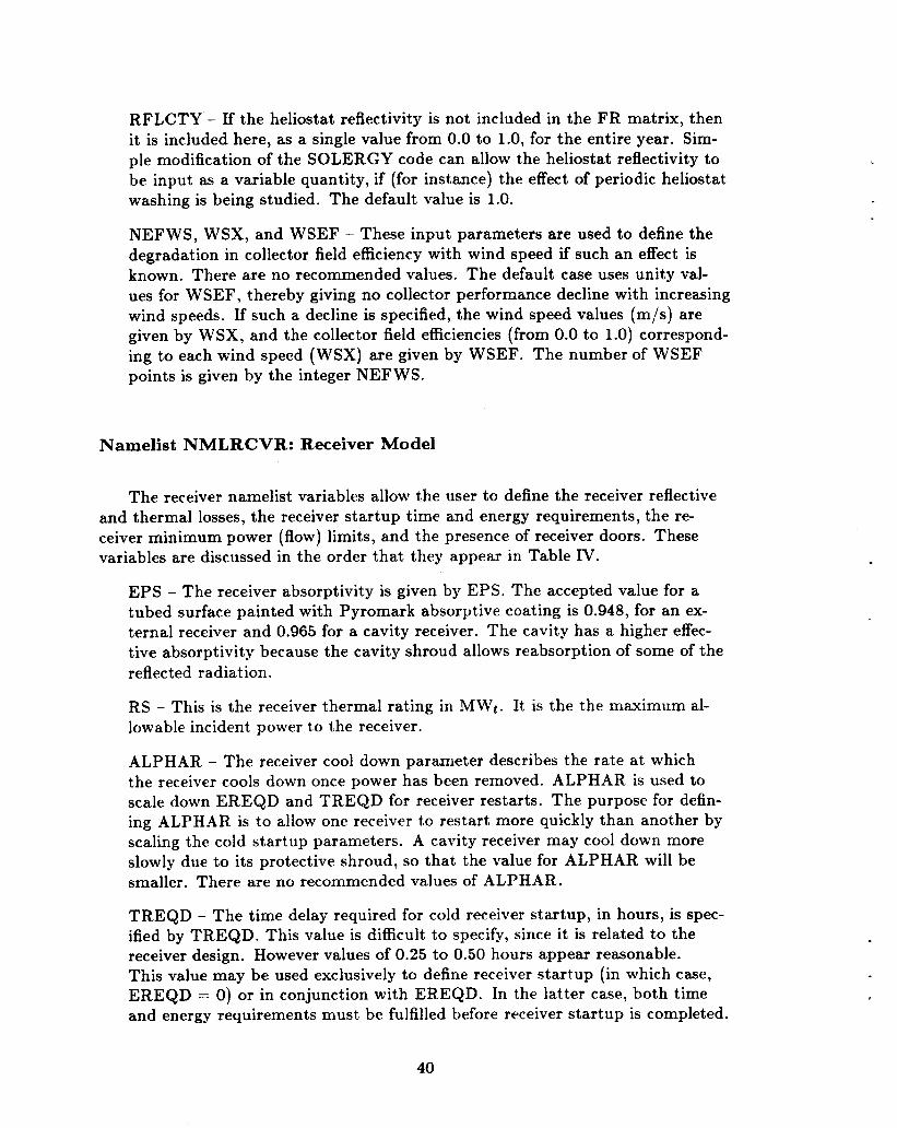
RFLCTY - If the heliostat reflectivity is not included in the FR matrix, then it is included here, as a single value from 0.0 to 1.0, for the entire year. Sim- ple modification of the SOLERGY code can allow the heliostat reflectivity to be input as a variable quantity, if (for instance) the effect of periodic heliostat washing is being studied. The default value is 1.0.
NEFWS, WSX, and WSEF - These input parameters are used to define the degradation in collector field efficiency with wind speed if such an effect is known. There are no recommended values. The default case uses unity val- ues for WSEF, thereby giving no collector performance decline with increasing wind speeds. If such a decline is specified, the wind speed values (m/s) are given by WSX, and the collector field efficiencies (from 0.0 to 1.0) correspond- ing to each wind speed (WSX) are given by WSEF. The number of WSEF points is given by the integer NEFWS.
Namelist NMLRCVR: Receiver Model
The receiver namelist variables allow the user to define the receiver reflective and thermal losses, the receiver startup time and energy requirements, the re- ceiver minimum power (flow) limits, and the presence of receiver doors. These variables are discussed in the order that they appear in Table IV.
EPS - The receiver absorptivity is given by EPS. The accepted value for a tubed surface painted with Pyromark absorptive coating is 0.948, for an ex- ternal receiver and 0.965 for a cavity receiver. The cavity has a higher effec- tive absorptivity because the cavity shroud allows reabsorption of some of the reflected radiation.
RS - This is the receiver thermal rating in MWt. It is the the maximum al- lowable incident power t,o t,he receiver.
ALPHAR - The receiver cool down parameter describes the rate at which the receiver cools down once power has been removed. ALPHAR is used to scale down EREQD and TREQD for receiver restarts. The purpose for defin- ing ALPHAR is to allow one receiver to restart more quickly than another by scaling the cold startup parameters. A cavity receiver may cool down more slowly due to its protective shroud, so that the value for ALPHAR will be smaller. There are no recommended values of ALPHAR.
TREQD - The time delay required for cold receiver startup, in hours, is spec- ified by TREQD. This value is difficult to specify, since it is related to the receiver design. However values of 0.25 to 0.50 hours appear reasonable. This value may be used exclusively to define receiver startup (in which case, EREQD = 0) or in conjunction with EREQD. In the latter case, both time and energy requirements must be fulfilled before receiver startup is completed.
40

EREQD - The energy required for a cold receiver startup, in MWht, is spec- ified by EREQD. This variable may be used exclusively to define receiver startup (in which case TREQD = 0) or in conjunction with TREQD. In the latter case, both time and energy requirements must be fulfilled before re- ceiver startup is completed.
RMF - The minimum acceptable flow fraction through the receiver is defined by RMF. Current designs place this value from 0.10 to 0.25 of maximum flow. Physically, RMF represents the ratio of the minimum flow to full flow with which the receiver can operate and still produce rated conditions at the out- let. It is used in SOLERGY to define the minimum incident power level with which the receiver can operate.
IFILL - The type of receiver, with doors or without, is defined by IFILL. A value of one defines a receiver with doors; a value of two defines a receiver without doors. The effect of IFILL is to determine whether the receiver must shut down during periods of low insolation or whether it can go into the hold mode, thereby avoiding the receiver startup procedure if the insolation level is restored.
Table IV. NMLRCVR Namelist Variables
EPS - Receiver absorptivity RS ALPHAR TREQD EREQD RMF IFILL - Receiver door flag
- R.eceiver thermal rating (MWt) - Receiver cool down parameter (hours-') - Time delay for receiver startup (hours) - Energy required for receiver startup (MWthr) - Receiver minimum flow fraction
Namelist NMLPIPE: Piping Model
The piping model namelist variables define the energy lost from the working fluid between the receiver and thermal storage as a function of ambient tempera- ture. This loss is quite small.
Table V. NMLPIPE Namelist Variables
NXLP TXLP
YXLP
- Number of elements in the temperature vector - Vector of ambient temperature points for spline fit, in
- Vector of corresponding loss coefficients. ascending order ( ' C)
4 1
I
___I
YXLP - These values (from 0.0 to 1.0) describe the fraction of power lost during transmission through the piping. They are used to obtain the power loss through the plant piping as a function of ambient temperature. There are no recommended values. The default values from Reference 1 were used- their origin is unknown.
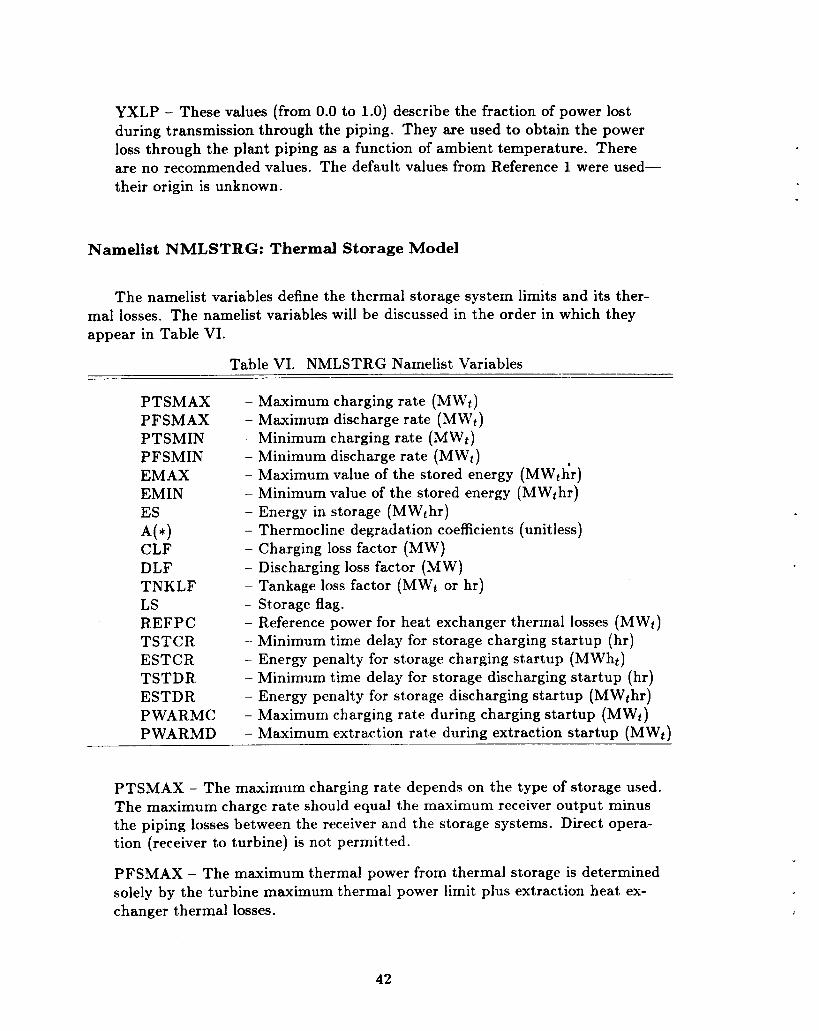
Namelist NMLSTRG: Thermal Storage Model
The namelist variables define the thermal storage system limits and its ther- mal losses. The namelist variables will be discussed in the order in which they appear in Table VI.
Table VI. NMLSTRG Namelist Variables
PTSMAX PFSMAX PTSMIN PFSMIN EMAX EMIN ES
CLF DLF TNKLF LS REFPC TSTCR ESTCR TSTDR ESTDR PWARMC PWARMD
A(*)
- Maximum charging rate (MWt) - Maximum discharge rate (MWt) - Minimum charging rate (MWt) - Minimum discharge rate (MWt) - Maximum value of the stored energy (MWth'r) - Minimum value of the stored energy (MWthr) - Energy in storage (MWthr) - Thermocline degradation coefficients (unitless) - Charging loss factor (MW) - Discharging loss factor (MW) - Tankage loss factor (MWt or hr) - St>orage flag. - Reference power for heat exchanger thermal losses (MWt) - Minimum time delay for storage charging startup (hr) - Energy penalty for storage charging startup (MWht) - Minimum time delay for storage discharging startup (hr) - Energy penalty for storage discharging startup (MWthr) - Maximum charging rate during charging startup (MWt) - Maximum extraction rate during extraction startup (MWt)
PTSMAX - The maximum charging rate depends on the type of storage used. The maximum charge rate should equal the maximum receiver output minus the piping losses between the receiver and the storage systems. Direct opera- tion (receiver to turbine) is not permitted.
PFSMAX - The maximum thermal power from thermal storage is determined solely by the turbine maximum thermal power limit plus extraction heat ex- changer thermal losses.

..
PTSMIN - The minimum charging rate depends on the type of thermal stor- age system. If a direct storage system is used, the minimum charge rate is functionally set by the minimum receiver output. However, a minimum charge rate of zero may be adequate unless there is a minimum flow required by the storage system itself. If an indirect storage system is used, the charg- ing heat exchanger design will determine the minimum charging rate. If little is known about the charging heat exchanger design, a minimum charging rate of one tenth of the maximum charge rate is a good rule-of-thumb.
PFSMIN - The minimum thermal storage discharge rate represents the ex- traction heat exchanger (steam generator system) turn-down ratio. From 10 to 25% of PFSMAX appears reasonable. Caution: PFSMIN must be less than or equal to TPFSL*TMFS or the turbine will not be allowed to start.
EMAX - The maximum energy capacity of thermal storage is determined by the designer based on the plant requirements, the relative cost of storage, and the extra collector field and receiver capacity required to provide storage with energy. DELSOL system designs can be used to define the storage size for a given solar multiple. The equation below may also be used, with caution, if no better information is available:
EMAX = 13.9 In (z) * PFSMAX (4)
where SM is the plant solar multiple. This equation is good only for solar multiples from 1.25 to 3.5 and for non-thermocline storage. If thermocline storage is modeled, the energy in storage must be referenced to the ambient temperature because of the tank thermal loss equation requirements. In the case of thermocline storage, EMAX is calculated as follows:
Eh4AX = 13.91n (E) * PFSMAX + EREF 1.18 ( 5 )
where EREF is t,he energy contained in the storage bed between the ambient temperature, Tamb, and the “cold” temperature in storage, Tcold:
where p and cp are the thermocline bed average density and specific heat re- spectively. See Appendix E for more discussion of this point. When subrou- tine MAXOUT is used, larger values of EMAX than calculated from Equa- tions 4 and 5 will result in higher energy values. Of course, larger storage sizes will also increase the plant cost. The optimal storage size (EMAX) will depend on the cost of storage and the increase in value provided by the addi- tional storage.
43

EMIN - The minimum stored energy is determined by the plant thermal en- ergy requirement during standby. There is no easy way to determine this value if a plant design is not available. An informed guess may be necessary. If thermocline storage is modeled, the minimum stored energy must be refer- enced to the ambient temperature (see Appendix E).
ES - The “instantaneous” energy in storage appears in the namelist so a user may set it as an initial condition. The value of ES should be between EMIN and EMAX.
A(l) , A(2), A(3)-These coefficients are used to determine the useful energy lost due to heat conduction and convection across the thermocline in a ther- mocline storage tank. The form of the heat loss equation is:
TPLBTC = A(l) + A(2) * ES + A(3) * ES2 (6)
There are no suggested values for these coefficients.
CLF - The charging loss factor is used to determine the charging heat ex- changer and piping network heat loss rates (MWt). The charging loss factor is used as follows:
Direct Storage (no heat exchanger):
TPLDC = CLF
Indirect Storage (charging heat exchanger present) :
TPLDC = CLF * ( PTSMAX)’ REFPC
(7)
Equation (8) assumes that the heat losses scale by the heat exchanger maximum thermal power capacity to the third power. The reference heat exchanger power, REFPC = 264 MWt, and the recommended value of 0.14 h4Wt for CLF is based on the Babcock and Wilcox molten salt steam generator repodg). There is no recommended value for CLF when used to determine the charging heat losses for direct storage.
DLF - The extraction (discharging) loss factor is used similarly to the charg- ing loss factor for indirect storage. It is assumed that thermal storage always discharges its energy through a heat exchanger. The recommended value for REFPC and DLF are 264.0 MWt and 0.14 MWt, respectively.
44
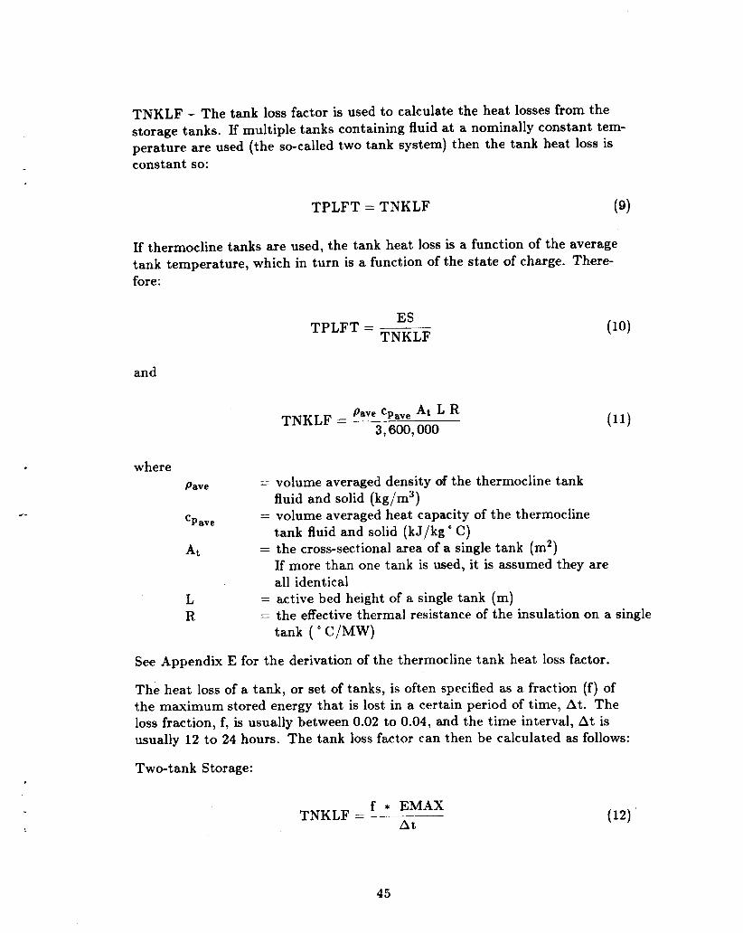
a-
TNKLF - The tank loss factor is used to calculate the heat losses from the storage tanks. If multiple tanks containing fluid at a nominally constant tem- perature are used (the so-called two tank system) then the tank heat loss is constant so:
TPLFT = TNKLF (9)
If thermocline tanks are used, the tank heat loss is a function of the average tank temperature, which in turn is a function of the state of charge. There- fore:
and
where
ES TNKLF TPLFT =
Pave CP ave At L R 3,600,000
TNKLF =
Pave
'pave
At
= volume averaged density of the thermocline tank
= volume averaged heat capacity of the thermocline
= the cross-sectional area of a single tank (m2)
fluid and solid (kg/m3)
tank fluid and solid (kJ/kg O C)
If more than one tank is used, it is assumed they are all identical
L R
= active bed height of a single tank (m) = the effective thermal resistance of the insulation on a single
tank ( 'C/MW)
See Appendix E for the derivation of the thermocline tank heat loss factor.
The heat loss of a tank, or set, of tanks, is oftmen specified as a fraction (f) of the maximum stored energy that is lost in a certain period of time, At. The loss fraction, f, is usually between 0.02 to 0.04: and the time interval, At is usually 12 to 24 hours. The tank loss factor can then be calculated as follows:
Two-t ank Storage:
f * EMAX At TNKLF =

Thermocline Storage:
At EMAX TNKLF = -
f EMAX - EMIN
LS - This directs the storage subroutine to use relations for a direct system, LS = 1; a thermocline system, LS = 2; or a storage system with an interfluid charging heat exchanger, LS = 3.
REFPC - This is the reference thermal power for computing the heat ex- changer heat losses. See CLF and DLF for more information. The recom- mended value of REFPC is 264.0 MWt.
TSTCR - The time delay before rated operation can occur after initiating charging startup is closely tied to the charging loop design and operating method. Therefore, it is extremely difficult to provide a recommended value. However, based on Solar One experience, the charging loop startup delay can range from 0.25 to 1.0 hour depending on the initial state of the charging heat exchangers. For a direct storage system (no charging heat exchangers), the charging startup time may be included as part of the receiver startup time. In this case, TSTCR = 0.
ESTCR - The energy penalty for charging loop startup represents the energy absorbed by the charging loop in bringing it to rated temperature. There is no recommended value.
TSTDR - The time delay before rated operation can occur in the extraction loop is closely tied to the extraction loop design and operating method. The default value of 0.25 hour is felt to be a reasonable estimate.
ESTDR - The energy penalty for extraction loop startup represents the en- ergy absorbed by the extraction loop in bringing it to rated temperature. There is no recommended value.
PWARMC - The maximum startup power level (MWt) for the charging loop is based on the heat exchanger and piping network design. The thermal power is limited during startup to avoid excessive thermal stresses during the transition to operating temperatures. For a system in which the receiver fluid is identical to the storage fluid, this value should be large (i.e., equal to RS) in order to remove any charging delay since charging heat exchangers do not exist. For a system with a charging heat exchanger, a value from 10 to 25% of RS seems reasonable.
The user is cautioned against specifying values of PWARMC that are less than the minimum flow limits of the receiver (RS * RMF or PTSMIN) when the direct storage option, LS = 1 or 3, is invoked. This error will prevent the receiver from ever operating since the charging heat exchanger cannot be started because the flow rate required for its warm-up cannot be achieved.
46

e-
PWARMD - The maximum startup power level (MWt) for the extraction loop is based on the heat exchanger and piping network design. The thermal power is limited during startup to avoid excessive thermal stresses during the transition to operating temperatures. There is no recommended value; how- ever, a value from 10 to 25% of the turbine thermal rating seems reasonable.
Namelist NMLTRBN: Turbine Model
The namelist variables in NMLTRBN describe the turbine, including its size, conversion efficiency, startup characteristics, and, for the simplified dispatch strat- egy, startup requirements. These input variables are defined in Table VII.
Table VII. NMLTRBN Namelist Variables
TBHWS TBWCS SDH SD W SDC RDH RDW RDC TPFSL TMFS ESMINl
ESMIN2
ESMAXl
ESMAX2
NREPSS
NCEPSS
REPSS
CEPSS
FEPSS
- Time between hot and warm startup (hr) - Time between warm and cold startup (hr) - Hot turbine synchronization delay (hr) - Warm turbine synchronization delay (hr) - Cold turbine synchronization delay (hr) - Hot turbine ramp delay (hr) - Warm turbine ramp delay (hr) - Cold turbine ramp delay (hr) - Thermal power for rated turbine operation (MWt) - Minimum turbine flow fraction (0.0 to 1.0) - Minimum storage energy level for turbine start, peak
period, receiver operating (Mb'thr) - Minimum storage energy level for turbine start, peak
period, receiver not operating (MWthr) - Storage level at which turbine must be started,
receiver operating (MWthr) - Storage level at which turbine must be started,
receiver not operating (MWthr) - Number of rows in FEPSS matrix (no. of wetbulb
temperatures) - Number of columns in FEPSS matrix (no. of
fractions of rated power) - Row vector of fractions of rated power for bicubic spline
(0.0 to 1.0). Must be NCEPSS values in ascending order. - Column vector of wet bulb temperature values ( ' C) for
bicubic spline. Must be NREPSS values in ascending order. - Matrix values for thermal to electric conversion efficiency
(0.0 to 1.0). Order is import,ant: all values in column 1, followed by all values in column two, etc. (NCEPSS by NREPSS)

TBHWS - The default time between a hot and a warm turbine startup is cur- rently set to 12.0 hours. This means that a turbine startup within 12 hours of the last turbine shutdown is treated as a hot startup. The value of TBHWS is from STEAEC,(') as are the values of TBWCS, SDH, SDC, RDH, RDW, and RDC. Their origin is otherwise unknown. Other turbine startup charactistics can be used.
TBWCS - The default time interval between a hot and a cold turbine startup is 72.0 hours. This means that a turbine startup within 12 to 72 hours of the last turbine shutdown is treated as a warm startup. After 72 hours of shut- down, the turbine will undergo a cold startup.
SDH, SDW, and SDC - The default hot, warm, and cold turbine synchro- nization time delays are 0.20, 0.24, and 0.40 hours, respectively. These values cause one time step delay for the hot and warm turbine synchronization and two time steps delay for the cold turbine synchronization if the time step is fifteen minutes. No electrical power is generated during these intervals.
RDH, RDW, and RDC - The hot, warm, and cold turbine ramp delays are 0.55, 1.10, and 3.30 hours, respectively. These values define the time required to ramp the turbine up to full power. Electrical power is generated at a re- duced rate during this interval.
TPFSL - The thermal power required by the turbine for rated operation is defined by TPFSL. This value can be determined by dividing the gross elec- t.rica1 power output of the turbine by its maximum thermal to electric conver- sion efficiency. In a properly designed plant, TPFSL is less than PFSMAX.
TMFS - The minimum fraction of full power at which the turbine is permit- ted to operate is expressed by TMFS. This value is dependent on the turbine being modeled; 0.25 is a reasonable value.
ESMINl sets the minimum value of storage energy a t which the turbine can be started during periods of rated receiver operation. It is typically a low value, perhaps 2-10% of the maximum thermal storage capacity. The as- sumption is that if the receiver is operating at rated conditions, energy will continue to be sent to thermal storage and the turbine startup will be success- fully completed without completely exhausting the stored energy.
ESMAX1 sets the level of storage energy at which turbine startup must be initiated, even if the time of day is not within an on-peak period. The value chosen for this variable will dictate whether energy will be discarded while awaiting the beginning of the on-peak period. If ESMAXl is a low value (e.g. equal to ESMINl) with respect to the maximum storage capacity, the tur- bine will run essentially whenever energy is coming from the receiver. This is a sunfollowing dispatch mode; it maximizes the net electricity produced by the plant. The revenue generated by the sale of this electricity will likely be less than any other dispatch scheme. When ESMAXl is chosen to be greater
48

.-
than ESMINl, the turbine startup is delayed until thermal storage reaches the level specified by ESMAXl (outside of the on-peak power period) or ESMIN1 (within the on-peak power period). In a properly specified plant, ESMAXl should never be less than ESMINl.
If GONOGO detects that the receiver is not in rated operation, it branches to allow ESMIN2 and ESMAX2 to control turbine startup.
ESMIN2 sets the minimum storage energy level at which the turbine can be started during periods of non-rated receiver operation. Since the receiver is not operating at rated conditions, it may not be assumed that a contin- ual stream of energy will be available for power generation. Thus, the value of ESMIN2 should be greater than that for ESMINl to prevent depletion of stored energy during turbine startup. To avoid excess turbine starts, ESMIN2 should be equal t,o the energy required for an hour or two of full power tur- bine operation.
ESMAX2 - Likewise, ESMAX2 sets the maximum storage energy level at which the turbine must be started when the receiver is not at rated opera- tion, regardless of the generating period. It is recommended that the value for ESMAX2 be chosen close to the maximum storage capacity.
ESMINl, ESMIN2, ESMAX1, and ESMAX2 are used with subroutmine GONOGO (IDISP = 1) only.
NREPSS, NCEPSS, CEPSS, and FEPSS - These values are used to obtain the turbine thermal-to-electric conversion efficiency as a function fo ambient wetbulb temperature and mass flow fraction. The default values are from Ref- erence 10 and are listed in the sample problem in Appendix B.l.
Namelist DISPATCH
The variables in the DISPATCH namelist allow selection of either the simpli- fied turbine dispatch strategy (turbine controller subroutine GONOGO) or the value maximizing turbine dispatch strategy (subroutine MAXOUT).
Table VIII. DISPATCH Namelist Variables
IDISP
TSTUR PSTFR
IDF1, IDF2
- Dispatch strategy selection: 0 for GONOGO and
- Estimated average time for turbine startup (hr) - Estimated fraction of rated turbine power output (TPFSL)
during TSTUR (0.0 to 1.0) - Print dispatch strategy trace (MAXOUT option) to output
unit 5 (file DISPAT.TRC) from day IDFl to day IDF2.
1 for MAXOUT
49

IDISP - If MAXOUT is selected (IDISP = l), then the next input variables are used. TSTUR and PSTFR provide information to the subroutine which attempts to predict the energy output for the day.
TSTUR can to estimated as (TSTDR or ESTDR/PWARMD) plus the sum of the turbine synchronization and ramp delays. PSTFR can be estimated as (TPFSL * TSTUR)-' * [(ESTDR or TSTDR * PWARMD) + (turbine synchronization delay) * TPFSL * TMFS + (turbine ramp delay) * TPFSL t 0.5).
IDF1, IDF2 - If no dispatch tracing is desired, then select any values for IDFl and IDF2 such that IDFl is greater than IDF2.
Namelist PRNTOUT: Output Selection
The values selected for the PRNTOUT namelist determine the beginning and ending days for which the output file will be produced. The level of detail for the output file, SOLOUT.PRT (unit 9), is also specified.
Table IX. MAXOUT Namelist Variables
MFLAG NDAF
NDAL
- Output detail print flag with values from 0 to 4. - First day to be printed with MFLAG level of information.
- Last day of the run; default is day 366. Default is day 1.
MFLAG = 0: component efficiencies are printed.
Minimal output-the annual plant performance summary and
MFLAG = 1: page for NDAF through NDAL is printed.
In addition to the previous level of detail, a daily summary
MFLAG = 2: In addition to the previous level of detail, the power flow and storage energy status for each time step for the days NDAF through NDAL is printed.
MFLAG = 3: efficiency and power to the receiver at each time step is printed.
In addition to the previous level of detail, the collector field
MFLAG = 4: the weather data tape is printed.
NDAF, NDAL - Note that NDAF denotes t,he first day for which output will be generated at the level of detail specified by MFLAG. It does not denote the first day for which SOLERGY calculations will be performed. (The run always begins with day 1.) However, NDAL denotes the last day for which
In addition to the previous level of detail, the input data from
50

output will be generated as well as the day on which the SOLERGY run will terminate.
51/52


3.2 SOLERGY Input Weather Data: SOLWEA.DAT
*.
The current form of the SOLERGY weather data is as an ASCII character file. The first line of the file is a header giving the year of the data. This value should begin in column one. The remaining lines of the file are the weather data. The minimal set of data that must be provided is the average direct normal inso- lation for each time step (DELT). The standard meteorological data required by SOLERGY are the following:
a. Direct normal insolation ( W/m2)
b. Wind direction (degrees with north equal to zero, increasing clockwise)
c. Wind speed (m/s)
d. Dewpoint temperature ( O F)
e. Barometric pressure (in. of Hg)
f. Dry bulb (ambient) temperature ( F)
A sample line of weather dat,a could look like the following:
842.42 83.00 4.00 45.00 29.60 72.00
Since the data are read by SOLERGY in free format, the entries on one line need to be separated by one or more spaces. There is no time mark on t,he data. It is assumed that the first line of data is for 12:OO a.m., January 1, and that subse- quent records are for each and every time step. No gaps are allowed in the data.
The user may add more data to each line as desired. Example, 9 are:
a. Heliostat reflectivity
b. Receiver absorptivity
c. Precomputed field efficiency
The first two would be used for simulating a time varying reflectivity or absoptiv- ity; the last if the user wished to reduce the computation required in SOLERGY by precomputing the field efficiency for each time step. Simple coding changes would be required to utilize these additional data.
If the dew point temperature data are not available for the site of interest, it is possible to compute the dew point knowing the relative or specific humidity, the ambient temperature, and using psychrometric tables such as those found in reference 11. If the user feels it appropriate, use of the following relationship for a constant 50% specific humidity is a third option:
53

Tdpt = 0.9017Tamb - 12.27
where: Tdpt = dewpoint temperature, F Tamb = ambient temperature, O F
This equation is valid over the range of ambient temperature from 10 O F to 120 F.
54

4.0 SOLERGY OUTPUT
- -
The minimum output from SOLERGY (MFLAG = 0) produces three pages of output. The first page is a summary description of the plant, including maximum power to the turbine, maximum storage charge rate, maximum heliostat field ef- ficiency, receiver thermal rating, thermal storage capacity, and the heliostat field size. The second output page provides a summary of the plant operation through- out the period of the run, nominally one year. The third page produces a sum- mary of “design point” and annual efficiencies for the collector field, receiver, pip- ing, and turbine subsystems. It also reports the overall plant efficiency. In addition to this output file (SOLOUT.PRT), SOLERGY produces two other output files: NMLOUT.PRT and EGEN.DAT. The NMLOUT.PRT file gives all namelist vlaues used in the current run. The EGEN.DAT file contains the input required for run- ning the program VALCALC (see Appendix C).
4.1 Annual Energy Summary
The annual energy summary, which is the minimum output generated in the SOLOUT.PRT file (unit 9), is now described in detail. Increasing levels of detail are produced by increasing the value of MFLAG up to 4. For MFLAG = 1, the daily values of the quantities described below are reported. For MFLAG = 2, the values of (1-4, 7-11, and 13) and the storage charge level are reported at each time step. For MFLAG = 3, the collector field efficiency and power to the receiver are printed at each time step. For MFLAG = 4, the weather data is printed for each time step. If the run was for less than one year, this output will represent the sum of daily operations, but will still be labeled as “yearly”.
1. Yearly Parasitics - Balance of Plant: Parasitic energy consumption occurring during plant operation for all subsystems except solar components and the tur- bine plant. Variable: YBOPPAR.
2. Yearly Parasitics - Turbine Plant: Parasitic energy consumption for operation of the turbine plant, which includes the turbine generator, condenser, and heat rejection systems. Variable: YTPPAR.
3. Yearly Parasitics - Solar Plant: Parasitic energy consumption for operation of the solar plant. This includes operation of the collector field, receiver, and ther- mal stor?ge charging and extraction subsystems. Variable: YSPPAR.

4. Yearly Parasitics - PM Shutdown: Parasitic energy consumption for nighttime and weather shutdown. Variable: YPMPAR.
5. Yearly Energy to Collector Field: Total energy that is available to the heliostat field. Dividing this number by the heliostat field size (m2) yields the annual in- solation (MWhr/m2). Variable: YDNI.
6. Yearly Energy to Receiver: Energy directed onto receiver from the heliostat field, including the effects of collector field efficiency and reflectivity. Not in- cluded are: energy that the receiver cannot use because the energy is too low, energy discarded because heliostats must be defocused to reduce power sent to storage, energy discarded because the power to the receiver exceeds receiver thermal rating, and energy not used due to plant outages. These quantities are accumulated in other variables. Variable: YPTR.
7. Yearly Energy to Working Fluid: Energy to receiver, reduced by receiver ther- mal and reflective losses. Variable: YPTWF.
8. Yearly Energy in Working Fluid: Energy to working fluid, reduced by piping thermal losses. Variable: YPWF.
9. Yearly Energy to Storage: All energy in the working fluid is sent to thermal storage (YPTS = YPVVF). Variable: YPTS.
10. Yearly Energy to Turbine from Storage: Energy sent to the turbine is YPTS reduced by the storage tank thermal losses, the charging and extraction heat exchanger thermal losses, and the energy required to start up the charging and extraction heat exchangers. Variable: YPFS.
11. Yearly Energy to Turbine: Energy sent to turbine equals energy from thermal storage (YPTT = YPFS). Variable: YPTT.
12. Yearly Surplus Energy to Receiver: Energy not used due to defocusing the he- liostats when the power to the receiver is greater than the receiver thermal rat- ing. Variable: YSPTR.
13. Yearly Surplus Energy to Storage at Receiver: Energy discarded because stor- age cannot accept the input: either storage is full or the charging heat ex- changer has not yet started. In both of these cases, t,he plant defocuses he- liostats and the net result is a reduction in power to the receiver. YSUPTR provides the amount of receiver energy discarded for these situations. Variable: YSUPTR.
14. Yearly Surplus Energy to Storage at Storagg: This energy is identical to the en- ergy given in YSUPTR: except that it is provided at the entrance to the stor- age system. The piping losses and receiver thermal and reflection losses have been removed from YSUPTR to obtain YSPTS. The lost energy at the storage interface is provided for information only. Variable: YSPTS.
56

15. Yearly Receiver Minimum Flow Losses: Receiver energy that is not collected because it is less than the minimum energy needed to operate the receiver. Variable: YPLRMF.
16. Yearly Receiver Start Time: Hours that the receiver spends in startup. Vari- able: YSTIME.
17. Yearly Weather Receiver Down Time: Hours that the receiver is nonopera- tional due to low insolation. Variable: YWTIME.
18. Yearly Forced Outage Time: Hours that the plant is nonoperational due to forced outage time. Variable: YFORC.
19. Yearly Scheduled Outage Time: Hours that the plant is nonoperational due to scheduled outage time. Variable: YSCHED.
20. Yearly Energy Loss Due to Outage Time: Energy that was not collected due to either forced or scheduled outages. Variable: YEOUTAGE.
21. ISTRT1: Number of times that the receiver begins startup within 45 minutes of sunrise. Variable: IBEGIN1.
22. ISTRT2: Number of times that the receiver begins startup within two hours of sunrise. Variable: IBEGIN2.
23. ISTRT3: Number of times that the receiver begins startup within three hours of sunrise. Variable: IBEGIN3.
24. ISTRT4: Total number of times that the receiver begins startup. Variable: IBEGIN4.
25. Number of Days Receiver did not Operate: Number of days during which there were no receiver starts. Variable: INOOP.
26. Number of Days Receiver Had More Than One Start: Variable: IMULTI.
27. Startup Energies: Receiver: Energy consumed during receiver startup. This energy appears in YPTR but is not passed on to YPTWF. Variable: YRSTRT.
Charging Heat Exchanger (Sodium to Salt Heat Exchanger): Energy consumed during startup of the charging heat exchanger. This energy is present in YPTS, but is not added to energy in storage. It is therefore a loss of useful energy in the storage tank. Variable: YCSTRT.
Extraction Heat' Exchanger: Energy consumed during startup of the extrac- t,ion heat exchanger. This energy appears as a loss of useful energy from stor- age, and is not passed on as YPFS. Variable: YESTRT.
Turbine: Energy consumed during startup of the turbine. This energy appears in YPTT, thermal power sent to the turbine, but does not result in electrical power generation. Variable: YTSTRT.
57

28. Turbine Starts: Number of times that a turbine start was initiated. Variable: ITSTART.
29. Turbine Starts Completed: Number of times that the turbine start was success- fully completed. A turbine start) cannot be completed when there is insufficient energy in storage and/or coming from the receiver through thermal storage to fulfill the turbine startup energy requirement. Variable: ION.
30. Yearly Gross Electricity from Turbine: Variable: YGPFT.
31. Yearly Net, Electricity from Turbine: Gross electricity from the turbine minus plant parasitics. Variable: YPFT.
32. Yearly Parasitics Furnished Plant: Sum of all plant parasitics. Variable: YPARN.
58

4.2 Annual Efficiency Calculations
...
Annual efficiencies are calculated for the collector field, receiver, piping, ther- mal storage, and turbine subsystems, as well as for the entire system. Accumulated energy values resulting from a SOLERGY simulation (whether or not it was for an entire year) are used to formulate these “annual” efficiencies. The calculation of each of these quantities is described below.
Collector Field Efficiency
The annual collector field efficiency, EFEC, is calculated as all the energy that the collector field could direct to the receiver divided by the annual insola- tion, YDNI. The numerator contains not only the energy actually used by the re- ceiver (YPTR), but also the energy that the receiver could not accept due to low insolation (YPLRMF), storage being full (YSUPTR), or the receiver rating be- ing exceeded (YSPTR) as well as energy that was not collected due to outage time (YEOUTAGE). The collector field efficiency shows the effects of heliostat reflectiv- ity, and cosine, shadowing, and blocking losses.
EFEC = (YPTR + YSTPR + YSUPTR + YPLRMF + YEOUTAGE)/YDNI (1)
Receiver Efficiency
The annual receiver efficiency, EFREC, is calculated as the energy that was transmitted to the working fluid divided by the energy incident on the receiver. Energy losses in the receiver are due to reflection, thermal emission, and convec- tion, as well as due to receiver startup.
EFREC = YPTWFjYPTR (2)
Piping Efficiency
The annual piping efficiency, EFPIPE, is calculated as the energy in the work- ing fluid after passing through the piping, YPWF, divided by the energy collected
59

by the receiver, YPTWF. The piping efficiency reflects the effect of thermal loss in the piping, which is generally quite small.
EFPIPE = YPWFjYPTWF (3)
Thermal Storage Efficiency
The annual thermal storage efficiency, EFTS, is calculated as the thermal en- ergy that storage delivers to the turbine, YPTT, divided by the energy sent to stor- age (YPTS = YPWF). This efficiency reflects the effects of storage tank thermal losses and startup of the charging and extraction heat exchangers.
EFTS = YPTT/YPTS (4)
Electrical Power Generation System Efficiency
The annual electrical power generation subsystem efficiency, EFEPGS, is cal- culat,ed as the gross electrical energy generated by the turbine, YGPFT, divided by the thermal energy delivered to the turbine by thermal storage (YPTT). The EPGS efficiency shows the effect of the turbine thermal to electric conversion effi- ciency as well as turbine startup losses.
EFEPGS = YGPFTjYPTT (5 )
Plant Efficiency
The overall annual plant efficiency, EFTOT, is calculated as the net electri- cal energy generated by the turbine divided by the annual insolation. The overall system efficiency represents the effects of all subsystem losses, outage time, and 24-hour plant parasitic loads.
EFTOT = (YGPFT - YPARN)/YDNI (6)
where:
YPARN YDNI
= total plant parasitics, 24-hour basis, MW, hrs. = total annual insolation available to the plant.
60

APPENDIX A: SOLERGY SUBROUTINE DESCRIPTION
Appendix A contains descriptions of all subroutines contained in SOLER GY. Section A.l provides a very brief description of each subroutine and Section A.2 gives more detailed information about major portions of the SOLERGY code. The purpose of Section A.2 is to provide information for the user interested in understanding the code in sufficient depth to make modifications to it.
A.l Summary Description of SOLERGY Subroutines
Subroutine INPU T1
The subroutine INPUT1 initializes all namelist input variables via either the default data st.at,ements or new values read from the namelist input file SOLNML.DAT, or a combination thereof. The default values represent a 100 MW, plant with a solar multiple of 1.2. The receiver fluid and thermal storage medium are both molten salt. Thermal storage is sized to provide 1.25 hours of rated power generation when it is fully charged and the receiver is not operating.
Subroutine COEF
The subroutine COEF is deactivated in SOLERGY. COEF should be reac- tivated if it desired to use IMSL library routines for generating two-dimensional splines for interpolating the two-dimensional input matrices. Reactivation consists of removing the ‘‘C‘s ”in column 1 of the IBCCCU call. The subroutine COEF calls IBCCCU, an interpolatory natural bicubic spline routine to generate matri- ces representing collector field efficiencies. In order to produce a self-contained code, the subroutine TSPLIN was written. SOLERGY is therefore able to run using only software which is in the public domain.
Subroutine INPUT2
The subroutine INPUT2 reads the input weather data file SOLWEA.DAT. This file, in ACSII format, contains values for direct normal insolation, wind di- rection, wind speed, dew point temperature, station pressure, and dry bulb tem-

perature. The subroutine calculates the wet bulb temperature and obtains the solar azimuth and elevation values from the subroutine SUNPOS.
Subroutine SUNPOS
The subroutine SUNPOS calculates the local azimuth and elevation of the sun at a specified geographic location and time.
Subroutine COLF
The subroutine COLF is the collector field model. It calculates the power to the receiver from the collector field (PTR(K)) as a function of the direct normal insolation, the field size, and the field efficiency.
Subroutine EFFIC
The subroutine EFFIC calculates the collector field efficiency as a funct.ion of solar azimuth and elevation angles. It includes the effects of heliostat, reflectivity and wind speed on field efficiency. EFFIC also determines if ambient conditions will permit operatlion of the collect,or field. Ambient conditions which can effect operation of the collector field are solar elevation angle, wind speed, and dry bulb temperature.
Subroutine EFWS
The subroutine EFWS calculates the effect of wind speed on collector field efficiency using the cubic spline routines SPLIFT and SPLINT.
Subroutine RCVR
The subroutine RCVR is the receiver model. It determines the mode of re- ceiver operation (rated, derated, holding, shutdown, or starting up) based on the current thermal power available from the collector field and the previous status of the receiver.
62

Function XLR
The function XLR is called by the subroutine RCVR to calculate the receiver thermal losses due to reradiation, convection. and conduction as a function of wind speed.
Subroutine PIPE
The subroutine PIPE models the transmission of the working fluid from the receiver to the thermal storage tank.
Function XLP
The function XLP is used in the working fluid transmission model to deter- mine conduction and convection losses in the piping as a function of dry bulb temperature.
Subroutine GONOGO
The subroutine GONOGO is the turbine operational controller. GONOGO monitors the energy level in the thermal storage tank. When a specified level is reached, the turbine startup is initiated. GONOGO continues to operate the tur- bine at rated conditions whenever possible. The turbine is shut down when there is 110 energy available from thermal storage.
Subroutine MAXOUT
The subroutine MAXOUT is the alternate turbine operational controller. SOLERGY uses either GONOGO or MAXOUT for turbine control. The DISPATCH namelist, input variable IDISP determines which of the two tur- bine controllers will be activated. MAXOUT attempts to maximize the value of solar-generated electricity by running the turbine during high value periods. The current default payment schedule is defined by the SCE Schedule TOU-8 (14). MAXOUT may select derated turbine operation and it may shut the turbine down before thermal storage is empty in order to carry thermal storage energy over into another, more valuable, generating period.

Function EPSS
The function EPSS uses a bicubic spline to compute t.he gross thermal to elec- tric conversion efficiency of the turbine as a function of wet bulb temperature and mass flow fraction of the power from storage.
Subroutine STRG
The subroutine STRG is the thermal storage system model. It receives the desired charge and discharge commands from the receiver and the turbine oper- ational controller. If possible, STRG complies with these demands. If the charge rate is excessive or if storage is full, the surplus power to storage is calculated and the demand is revised. If the energy in storage is insufficient to supply a request to the turbine, the unavailable power from storage is calculated and the request is revised. The modes of thermal storage operation are standby, charge, discharge, and simultaneous charge and discharge.
Subroutine HANDLER
The subroutine HAXDLER is called if either of the storage variables SUPTS or UPFS are non-negative, that is, if the thermal storage system either cannot meet the demands from the tjurbine or if it cannot accept the power delivered by the receiver system. HANDLER calculates the required reductions in PTR (power delivered by the collector field): PTWF (power delivered by the receiver to the working fluid). and PWF (power in the working fluid after piping losses) when heliostat defocusing must be simulated.
Subroutine TRBN
The subroutine TRBN uses the power supplied from thermal storage as input, to the turbine. It calculates the electrical power generated by the turbine.
Subroutine PARASI
The subroutine PARASI calculates the plant parasitics depending upon the mode of plant operation. The operational parasitics are calculated for three ma- jor plant portions: the balance of plant, the turbine plant. and the solar plant. There are two equations for nonoperational parasitics: one is used for daily
64

weather outages and for nighttime shutdown and the other is used for the times when there is a scheduled outage or the plant has been on an extended weather outage.
Subroutine ADJPRE
The subroutine ADJPRE performs an adjustment of the insolation prediction to account for the insolation observed for the present time interval of the day. The adjustment is equal to the difference between the predicted and the observed insolation and is subtracted from the prediction for the remainder of the day. The magnitude of the resulting prediction is limited to the maximum clear sky inso- lation values calculated by the subroutine ALLEN. The subroutine ADJPRE as well as the subroutines ALLEN, PREDICT, and SCOVER are used only by the subroutine MAXOUT.
Subroutine ALLEN
The subroutine ALLEN is called at t,he beginning of each day. It calculates the maximum clear sky insolation possible for each time step that the sun is above the horizon. The resulting array, SUNMAX, is used to initialize the ar- ray SUNP at the beginning of the annual simulation and to limit the insolation prediction within the subroutine ADJPRE.
Subroutine PREDICT
The subroutine PREDICT is called once at the beginning of the day and then after each call to ADJPRE during the day. PREDICT uses the predicted insola- tion to estimate the amount of energy available from the receiver for the remain- der of the day until sunset, PHBT, and the amount of energy available from the receiver during the turbine startup period (PHBTS).
Subroutine SCOVER
The subroutine SCOVER is called at the beginning of each day. It calcu- lates SMAX, the maximum amount of thermal energy in storage for that day. SCOVER is explained in greater detail in Appendix A.2.

Subroutine SPLIFT
The subroutine SPLIFT is from the Sandia Mathematical Program Library(’). It fits an interpolating cubic spline to the N data points given in X and Y. It re- turns the first and second derivatives in YP and YPP. The resulting spline, de- fined by X, Y, and YPP, and its first and second derivatives may then be evalu- ated using SPLINT.
Subroutine SPLINT
The subroutine SPLINT is from the Sandia Mathematical Program Library(’). It evaluates a cubic spline and its first and second derivatives at the abscissas in XI. The spline, which is defined by X, Y, and YPP, may have been determined by SPLIFT or any other spline fitting routine that provides second derivatives.
Subroutine TSPLIN
The subroutine TSPLIN uses the one-dimensional spline fit routines SPLIFT and SPLINT to provide a two-dimensional spline fit.
66

A.2 Operational Details of Key SOLERGY Models
Location of the Sun: Subroutine SUNPOS
The amount of power redirected to the receiver by a heliostat field of fixed reflective surface area varies as the sun moves through the sky. Subroutine SUNPOS locates the sun in the sky above the modeled solar central receiver plant in spherical coordinates of azimuth and elevation as shown in Figure A-1. Subroutine SUNPOS also calculates the time of sunrise and sunset in local time which is useful for scheduling plant operations.
Subroutine SUNPOS was taken from reference 12. Additional coding which compensates for the elevation angle due to atmospheric refraction was taken from reference 13, wherein subroutine SUNPOS is referred to as SUNAEP. The method of converting solar time to local time was taken from reference 14.
Variables for Subroutine SUNPOS
There are four namelist variables for subroutine SUNPOS: LAT, LONG, ZONE, and IFLAGP. These variables were described in Section 3 of the text. There are seven input parameters passed to subroutine SUNPOS in the subrou- tine call statement:
YEAR - the year number (e.g., 1984),
DAY - the day number of the year starting with 1 for January 1,
XNHR - the time of the day in local time: hours, minutes (MIN), and sec- onds (SEC).
TA - ambient temperature (degrees F). Used in atmospheric refraction correc- tion calculation.
PRESSA - ambient pressure (millibars). Used in a.tmospheric refraction cor- rection calculation.
There are seven parameters that have a value returned by the subroutine SUTiPOS:
A - Azimuthal angle of the sun in degrees (positive is west of south).
E - Elevation of the sun (degrees).
EC - Elevation corrected for atmospheric refraction (degrees).
67
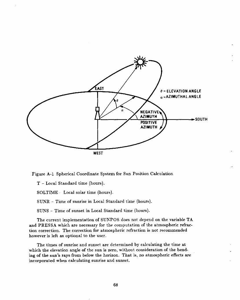
e = ELEVATION ANGLE a =AZIMUTHAL ANGLE
*SOUTH
WEST
.-
Figure A-1 Spherical Coordinate System for Sun Position Calculation
T - Local Standard time (hours).
SOLTIME - Local solar time (hours).
SUNR - Time of sunrise in Local Standard time (hours).
SUNS - Time of sunset in Local Standard time (hours).
The current implementation of SUXF’OS does not, depend on the variable TA and PR.ESSA which are necessary for the computation of the atmospheric refrac- tion correction. The correction for atmospheric refraction is not recommended however is left as optional to the user.
The times of sunrise and sunset are determined by calculating the time at which the elevation angle of the sun is zero, wit,hout consideration of the bend- ing of the sun’s rays from below the horizon. That is, no atmospheric effects are incorporated when calculating sunrise and sunset.
68

Receiver Operational Details: Subroutine RCVR
The decision whether to operate the receiver is made in the RCVR subrou- tine. Upon entry to t,he RCVR subroutine, the previous state of the receiver is checked. If the receiver was previously not shut down, then conditions are exam- ined to determine if the previous state (operation or startup) can continue. If the receiver was previously shut down, then conditions are examined to determine if startup is possible. If startup is not possible, then the shutdown time is allocated to regular nightime shutdown or weather outage. The communication variables of the receiver subroutine are described in Table A.1.
Table A.l Communication Variables of Subroutine RCVR
PTR(K) PTWF PLRMF
SPTR
IRSU
IRO
IDRO
IRSHUT
IHOLD
- Thermal power to the receiver, MWt - Thermal power to the working fluid - Receiver energy not collected because it is less than
the minimum energy the receiver can accept - Surplus power to receiver - power delivered to receiver
that is greater than receiver thermal rating - Receiver startup mode flag: 0 = receiver not in startup;
1 = receiver in startup - Receiver rated operation mode flag: 0 = receiver not in
rated operation; 1 = receiver in rated operation - Receiver derated operation mode flag: 0 = receiver not
in derated operation; 1 = receiver in derated operation - Receiver shutdown mode flag: 0 = receiver not shutdown;
1 = receiver shutdown - Receiver hold mode flag: 0 = receiver not in hold mode;
1 = receiver in hold mode
Upon entering the subroutine RCVR, the time of day is checked to determine if this is an operational time. The receiver is permitted to operate during the times between one half-hour after sunrise and one half-hour before sunset. The selection of these opera6onal times was arbitrary and can be changed if desired. If the current time is within the operational time band, then the power to the receiver is checked for determination of net positive power. The receiver is consid- ered to have net positive power if the incident power minus the reflective, convec- tive, and radiative losses is greater than the minimum receiver power limit. In the case of net positive power, the receiver is started up. Otherwise nighttime shut- down time is accumulated by the variable TRSHUT or weather outage time is ac- cumulated by the variable WTIME. However, in the case of a forced or scheduled outage, the time is not counted as weather outage. Any power that is not col- lected during this period of nonoperation is accumulated in the variable PLRMF.
When the receiver starts up, the variable IDAYOP is incremented by one, sig- nalling that a receiver startup is being initiated. Several other counters are also
69

examined, and if appropriate, are incremented. These counters accumulate the number of starts attempted within different intervals from sunrise. The variable IBEGINl indicates that the receiver start is within forty-five minutes of sunrise; the variable IBEGINZ indicates that the receiver start is within two hours of sun- rise; the variable IBEGIN3 indicates that the receiver start is within three hours of sunrise; and the variable IBEGIN4 indicates that the receiver is being started up, regardless of the time. These variables are for information only and may be modified to count any other significant startup events.
Either a time or energy requirement, or both, is specified for receiver startup in the input namelist. These requirements, EREQD or TREQD, are described more fully in Sections 2.2 and 3.0. These values are specified for a cold receiver. During an actual receiver startup, the time the receiver has been shut down is ac- counted for by describing the receiver initial state with EINIT and TINIT, which are dependent upon TRSHUT. The time and/or energy requirements which must be met are then TTOSTART and ETOSTART, the cold receiver requirement mi- nus the initial states. Completion of startup is signalled by the fullfilment of both the startup time and energy requirement.
There is one condition during which the startup will not proceed: the hold mode. Within the code, this mode is signalled by both the startup flag (IRSU) and the hold mode flag (IHOLD) being set. This mode is permitted only for receivers with doors (IFILL = 1). It is a time-limited state (three time steps) within which the receiver is allowed to exist if it would otherwise have to shut- down. If the receiver is in the hold mode and sufficient insolation for operation returns, the receiver is allowed to restart instantaneously. If, however, insolation does not return within the allotted time, the receiver is forced to shut>down just like a receiver without doors (IFILL = 2).
Thermal Storage System Details: Subroutine STRG
The storage subroutine interacts with the other subroutines of SOLERGY through the variables in Table A.2. Other variables mentioned in this section have been previously described (Section 3). The storage subroutine acts to sat- isfy the demands placed upon it by the receiver and the turbine controller subrou- tines. The demands of the receiver and turbine are communicated to storage by the values of PTS and PFS, respectively. A zero or negative value indicates that charging or extraction is to be halted if it is currently operating, or maintained inactive if that is the current status. A positive value indicates that charging or extraction is to be started if currently inactive, or continued if the function is currently active. In all but one case, a non-zero value of SUPTS or UPFS indi- cates that storage has completely satisfied the demands placed upon it. The one
70

.-
Table A.2 Communication Variables of the Subroutine STRG
PTS PFS SUPTS
UPFS
ES ITRNC
- Power sent to storage, MWt - Power delivered by storage, MWt - The amount of power sent to thermal storage
that is beyond its capability to accept, MWt - The amount of power requested from thermal
storage that can not be delivered, MWt - The energy in storage, MWthr - Indicates if storage is in transition from
charging inactive to charging active. 0 = in steady state, 1 = in transition.
- Indicates if storage is in transition from extraction inactive to extraction active. 0 = in steady state, 1 = in transition.
system is operating in. 0 = Inactive 1 = Charging only 2 = Extraction only 3 = Combined charging and extraction
ITRND
ISTSS - Indicates which steady state mode the storage
ISURP - Indicates which limit condition was exceeded when SUPTS or UPFS is non-zero.
0 = No problem 1 = Charge rate is less than minimum 2 = Charge rate exceeds maximum 3 = Extraction rate exceeds maximum 4 = Extraction rate is less than minimum
ITURNON - Indicates whether the turbine is to be turned on 0 = No 1 = Yes
exception is during the startup of the storage extraction function which will be discussed later.
Figure A-2 is a flow diagram showing the internal operation of the storage subroutine. The first section of the subroutine checks whether the charging power level is positive. If it is zero or negative, the thermal storage status is changed to reflect the shutdown of the dorage charging heat exchanger. The charging power level is then checked to determine whether it is within the maximum and mini- mum limits. If the charging thermal power is out of range, a value for SUPTS is calculated and the subroutine exited.
If the charging power checks are successful, the subroutine continues with the extraction power checks. If the extraction power level is equal to or less than zero, the thermal storage status is changed to reflect extraction loop shutdown.
71
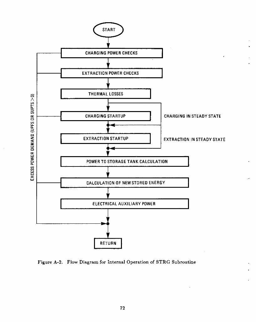
START Q
h
0 A
n
a
2 2 v)
0 v) LL
3
0 z I W 0 a
n - a
Y 2 v) v) W 0 x W
v CHARGING POWER CHECKS
I
EXTRACTION POWER CHECKS
. THERMAL LOSSES
CHARGING STARTUP
I EXTRA CTI 0 N STARTUP
CHARGING IN STEADY STATE
EXTRACTION IN STEADY STATE
1
POWER TO STORAGE TANK CALCULATION
CALCULATiON OF NEW STORED ENERGY I I ELECTRICAL AUXILIARY POWER
ri RETURN
Figure A-2. Flow Diagram for Internal Operation of STRG Subroutine
72

The extraction power is then checked to determine whether it is within the max- imum and minimum limits. If the extraction power is out of range, a value for UPFS is calculated and the subroutine exited.
The t,hird section contains the thermal loss calculations for the charging and extraction heat exchangers and for the thermal storge tank(s).
The fourth section handles the startup of the charging loop. If the charg- ing loop status is inactive and positive thermal power is delivered to the charg- ing loop, the thermal storage status variables are adjusted to show the charging loop is in transition. The code in this section first acts to redefine the maximum and minimum charging rates such that the net power delivered to the charging loop (PTS - TPLDC) does not exceed the charging heat exchanger startup rate (PWARMC). If (PTS - TPLDC) exceeds PWARMC, a value for SUPTS is cal- culated and the subroutine exited. If the net power delivered is within limits, the code then checks to see if the startup time and energy delay criteria have been met. If t.he criteria are satisfied, the charging transition flag is turned off and the storage status is set to indicate that the charging loop is active. These two changes will cause the charging transition code to be bypassed in subsequent calls to the storage subroutine.
The fifth section handles the startup of the extraction loop. If the extraction loop status is inactive and positive thermal power is demanded from the extrac- tion loop, the thermal storage status variables are adjusted to show the extraction loop is in transition (ITRND = 1). The code in this section then acts to redefine the maximum and minimum extraction rates such that the net power delivered to the turbine, PFS, is zero, and such that the energy extracted from the stor- age tanks is equal to the sum of the extraction heat exchanger startup rate and its thermal loss (PWARMD + TPLDD). The value for UPFS remains zero even though thermal storage is not providing the requested thermal power. The code then checks to see if the time and energy delay criteria for extraction heat ex- changer startup have been met. If the criteria are satisfied, the extraction transi- tion flag is turned off and the storage status is set to indicate that the extraction loop is active through ISTSS. These two changes will cause the extraction transi- tion code to be bypassed in subsequent calls to the storage subroutine.
The sixth section computes the thermal powers delivered to and extracted from the storage tanks under steady-state and transient conditions. The charging and extraction mass flow rates are also calculated.
The seventh section calculates the change in energy in the thermal storage t,anks according to Equation 13 in Section 2.2. If the new amount of energy in the storage tanks exceeds the maximum or minimum energy limit, a value for SUPTS or UPTS is calculated and the subroutine exited without updating the variable, ES, by the new value of stored energy. The values of PTS and PFS must be ad- justed and the subroutine reentered in order to change the stored energy value.

Subroutine HANDLER
The subroutine HANDLER is called only if an unsatisfied condition is de- tected in the storage subroutine. HANDLER performs the necessary adjustments to resolve this condition, which can result from an unacceptable power to storage from the receiver, an unacceptable request for power by the turbine, or an extrac- tion/ turbine startup condition.
The subroutine HANDLER is called in two specific situations. The first is if either of the storage values SUPTS or UPFS is non-zero, that is, if the thermal storage system either cannot accept the power delivered by the receiver subsys- tem (SUPTS # 0) or cannot supply the requested amount of power to the turbine (UPFS # 0). HANDLER calculates the required reductions in the appropriate power streams. If necessary, it back-calculates required reductions in power to the receiver (PTR), simulating heliostat defocusing. The variable ISURP is set to a value which corresponds to the particular condition that cannot be satisfied in the storage subroutine.
The second condition which will result in a call to HANDLER is startup of the storage extraction and turbine subsystems. This sets the flag ITURNON = 1, indicating that this subsystem is in a startup mode.
ISURP = 1
Power delivered to storage from the receiver is less than the minimum allow- able storage charge rate. Action: Shut the receiver down, or put a receiver with doors on hold.
The storage subroutine has determined that it cannot accept any of the power from the receiver because the power level is too low. The receiver is shut down, and power t*o storage (PTS) and powers to and in the working fluid (PTWF, PWF) are set to zero. A receiver with doors goes on hold and a receiver without doors shuts down. Power to the receiver (PTR(K)) is set to zero. The power lost due to this low insolation condition is accumulated as a receiver mini- mum flow loss (PLRMF). The storage subroutine is called again, with no power delivered by the receiver subsystem.
ISURP = 2
This condition can be caused by exceeding the maximum storage charge rate, by exceeding the storage charge rate allowed during startup of the charging heat exchanger or, by delivering more energy than storage can accept because it is full. Action: Reduce the receiver output.
The subroutine STRG has specified the quantity of power that it cannot ac- cept in the variable SUPTS, surplus power to storage. The power to storage,
74

PTS, is reduced by this amount, thus simulating a defocus of some heliostats. Corresponding reductions in powers to and in the working fluid (PTWF, PWF) and power to the receiver (PTR(K)) are back-calculated. The variable SUPTR, surplus power to the receiver, accumulates the amount of power which is dis- carded at the receiver interface.
A check is performed to determine if the subsequent conditions will still result in net positive power to the receiver. Three possibilities exist:
(2)
(22)
(iii)
There is still enough power for rated receiver operation (net positive power is being delivered by the receiver). The storage subroutine is called with the new value of power to storage, PTS.
There is enough power for derated receiver operation (net positive power is not delivered by the receiver, that is, the thermal equivalent of parasitic power for solar system operation exceeds the power collected by the receiver). The storage subroutine is called with the new value of PTS.
The power reduction will cause negative power to the receiver. The receiver is shut down. The storage subroutine is called with zero input from the re- ceiver, and the powers to and in the working fluid (PTWF, PWF) and power to the receiver (PTR(K)) are set to zero. The variable PLRMF accumulates the power which is discarded at the receiver interface.
ISURP = 9
The turbine demand exceeds the maximum storage extraction rate or storage cannot supply the turbine demand due to low level. Action: Reduce the turbine demand (PFS) .
The turbine has demanded more power than storage can supply. The storage subroutine sends the amount of power that it cannot supply in HANDLER in the variable UPFS, unavailable power from storage. HANDLER reduces the power demanded from storage, PFS, by UPFS. The subroutine GONOGO or MAXOUT is then called and, if necessary, a transition to a different turbine operating state is made. The section describing GONOGO describes more completely the logic involved in this decision. After returning from GOIVOGO, the storage subroutine is called with the revised power demand.
ISURP = 4
The turbine demands less than the minimum storage extraction rate or the storage tank is empty. Action: Eliminate the demand and shut the turbine down.
When the turbine demands less power than the minimum storage discharge rate or there is no energy in storage, the power requested from storage is elirni- nated. The subroutine GONOGO is called with the revised value, PFS = 0, and
75

the necessary transitions are made. Upon returning to HANDLER, the storage subroutine is called with the revised demands.
ITURNON = 1
The storage extraction heat exchanger and the turbine are in a startup mode. In this situation, the HANDLER subroutine detects when startup of the extrac- tion heat exchanger has been initiated. When it recognizes that the extraction startup has been completed, it allows the turbine warmup to begin.
This two-layered startup is necessary because the extraction heat exchanger startup requires that a request for power from storage be made in order to con- tinue the startup procedure. It will not, however, deliver power from storage un- til the extraction heat exchanger warmup has been completed. SOLERGY must recognize that returning PFS = 0 from the storage subroutine does not indicate that no power is available from storage, but that the extraction heat exchanger is actually preparing itself for power delivery. Therefore, the request of PFS must continue to be made until the extraction heat exchanger is warmed and is ready to supply power to the turbine for the second phase of this subsystem startup.
When HANDLER detects that ITURNON = 1 and ITRND = 0, the startup of the extraction heat exchanger is complete. The flag ICAN = 1 is set, indicat- ing that the turbine startup can begin. The subroutine GONOGO or MAXOUT is called. U’ith the flags ITURNON = 1 and ICAN = 1, GONOGO initiates the turbine startup. More details of the turbine startup are included in the GONO GO subroutine sect ion.
Subroutine SCOVER
SCOVER is called in the main program at the beginning of each day to cal- culate SMAX, the maximum amount of thermal energy in storage for the day. SMAX is calculated using the following assumptions:
1. Storage is empty at the beginning of the day, and
2. The turbine is started at the following t.ime:
Start t,ime = [(time at end of the on-peak period) - PHBT/TPFSL], where:
PHBT = predicted amount of energy collected by the receiver for the day, MWthr
TPFSL = turbine thermal energy consumption rate at full power, MWthr
76

For weekends and holidays, the end of the on-peak period is set (in the main pro- gram) to the time at sunset. SCOVER calls subroutine EFFIC to obtain values of receiver thermal output for each time step of the day.
Figure A-3 shows the receiver thermal power output, thermal power con- sumed by the turbine, and energy level in thermal storage calculated by SCOVER for a solar plant with solar multiple of 1.62 operating on a weekday in July. In the figure, thermal energy is expressed as the length of time that the turbine can be operated at maximum power using that amount of energy. Thermal power is normalized by the maximum thermal power, TPFSL, required by the turbine. As was typical of July 1984, the afternoon was cloudy, as shown by the sharp de- crease in receiver output after l PM. SMAX is identified in the figure as the max- imum thermal energy level in storage for the day.
The thermal storage capacity minus SMAX is the amount of excess, or carry- over storage, SCO1, that can be filled at the beginning of the day without causing overflow of storage later in the day, provided the actual insolation for the day to come is less than or equal to the predicted insolation that was used to calculate SMAX. If the actual insolation is greater than the predicted insolation the tur- bine may be started before the turbine startup time calculated in SCOVER. If the actual insolation is less than the prediction, then the turbine may be started later than anticipated, the turbine may be derated, or carryover storage may be used during the on-peak period.
With just the above definition of SMAX, the amount of thermal energy dis- carded does not go to zero for large thermal storage capacities. Therefore, the value of SMAX is increased within SCOVER, according to the following formula:
SMAX = SMAX + (1.0 - SM) j: HMAX * 3.0
SM is the solar multiple. The value of 3.0 was determined by trial and analysis of various runs of the computer program SUNBURN ('1. For the example of Figure A-3, the value of SMAX returned to the main program was 3.71 hours.
Subroutine MAXOUT
Subroutine MAXOUT is a version of subroutine GONOGO that has been modified to maximize the value of electricity generated by a solar plant. The net incre Lse in value that can be obtained by using the value-maximizing thermal en- ergy dispatch strategy of MAXOUT can be substantial, depending on the utility, the solar plant design, and the amount of additional t,hermal storage that may be required to allow the solar plant to regularly supply electricity during periods when demand for electricity is high. The high electricity value rates are not avail- able to a plant that does not supply electricity with sufficient regularity during high demand periods. Refer to Appendix C for a description of the calculation of electricity value.
77
-_I____)-- ._

. . . . . . . . . . . . . . . . . .
. . . . . . . . . . . . . . . . . . . . . . . . . . . . . .
. . . . . . . . . . . . . . . . . . . . . . . . . . . . . .
. . . . . . . . . . . . . . . . . . . . . . . . . . .
. . . . . . . . . . . . . . . . .
. . . . . . . . . . . . . . .
. . . . . . . . . . . . . . .
. . .
. . .
. . ~ . . . . . . . . . . . . . . . .
ia I2 f t n
. . . . . . . . . . . . . . .
. . . . . . . . . . . . . . . . . . . . .
. . . . . . . . . . . . . . . . . . . . . .
. ) ........................
0
xi 0
hl
0
cv
............................... ................................. c\i
0
0 .............. od
7
0 rd - 0
E si= L n
0 ‘3 s o
O E
.................... . . . . . . . . . . . . . . . . . . . . . . . . . .
m C
0
. . . . . . . . . . . . . . . . . . . . . . . . . . . . . o m r U
7 .- - 9 0 00
0 . . . . . . . . . rd
I I I1 I1 o o a
.. . . . . . . . . . . . . . . . . . . . . . . . . . . . .
t o I I
78

In this section, reasons for the variation in value rate of electricity are ex- plained. Then, details of the thermal energy dispatch strategy of MAXOUT are described. This dispatch strategy uses thermal storage to operate the turbine when the value rate of electricity is the greatest. Without thermal storage, the turbine can operate only when the sun is shining.
Variations in Value Rate of Electricity
A quantity of electricity generated by a solar plant is worth the same amount as that same quantity of electricity generated by any other plant(s). Therefore, if the generation cost of the electricity from the solar plant is the same as the gen- eration cost from any other plant(s), a utility will be indifferent to the source of electricity. Thus, the measure of value of an amount of electricity from a solar plant is the cost of generating that same amount of electricity, using other sources available to the utility. For example, if the cost of generating electricity using other sources is high, then the value of electricity generated by a solar plant will also be high.
The costs of generating electricity vary during a day for utilities that must satisfy a daily varying demand for electricity. Typically, utilities divide days into rate periods: on-peak periods correspond to periods when demand is greatest; mid-peak periods correspond to periods when demand is intermediate; and off- peak periods correspond to periods when demand is least. The difference in cost of electricity during these rate periods reflects the differences in type of plant and type of fuel used to generate electricity during these rate periods. Typically, baseload plants are run continuously throughout the day and exclusively during off-peak periods; in contrast, peaking plants are operated only during the on-peak periods. The cost of electricity generated by peaking plants is greater than the cost of electricity generated by baseload plants primarily because peaking plants are operated for much less time than baseload plants. Therefore, the capital costs of a peaking plant must be distributed over a much smaller amount of electricity. Also, peaking plants characteristically use more expensive fuels and operate with lower efficiency than baseload plants.
Details of the Thermal Energy Dispatch Strategy
The thermal energy dispatch strategy is a set of rules which are designed to run the turbine during the on-peak period in preference to the mid-peak or off- peak periods and to run the turbine during the mid-peak period in preference to the off-peak period. In addition to maximizing the operation of the turbine dur- ing the on-peak period, the dispatch strategy minimizes discard of solar thermal energy by using an insolation prediction to anticipate, and by operating the tur- bine to avoid, discard of thermal energy. This discard would occur during those periods when thermal storage is full and the receiver output is greater than the maximum turbine consumption rate. The dispatch strategy of MAXOUT is appli- cable for solar plants with varying field sizes and storage capacities.
79

At the beginning of each day, values of PHBT and the carryover storage en- ergy levels, SCO1, SC02, and SC03, are calculated based on the predicted inso- lation for the day (see Section 2.4(b) for a description of these variables). This insolation prediction is contained in array SUNP(*). For each time step, be- tween the times of sunrise and sunset, subroutine ADJPRE is called to modify the weather prediction for the present time step and for each of the time steps for the rest of the day. This updated insolation prediction is contained in ar- ray SUNAP(*). Then, subroutine PREDICT is called to calculate new values of PHBT and PHBTS based on the modified weather prediction. PHBTS is the pre- dicted amount of energy collected by the receiver during the turbine startup p e riod. The rules of the dispatch strategy are organized in two groups, depending on whether the turbine is not running or is running.
Turbine Not Running
If the turbine is not running, the dispatch strategy must decide if the turbine should be started. If the present time is before the on-peak period of any day (for holidays and weekends, the main program sets the beginning and the end times of the on-peak period to sunset), and if the following four conditions are satisfied, then the turbine will be started.
1. The energy level in storage, ES, exceeds SCOl,
2. The sum of PHBT and (ES - SCOl) must be greater than the amount of en- ergy required to start and run the turbine at full power until the end of the on-peak period,
3. The sum of PHBTS and (ES - SCO1) must, be greater than the amount of energy required to start the turbine, and
4. (ES - SCO1) must be sufficient to start and run the turbine at full power un- til 1.5 hours aft,er sunrise. This condition insures that carryover storage will not be used to run the turbine before sunrise.
If the present time is within the turbine startup time, TSTUR, of the on-peak period, if today is not a holiday or a weekend, and if the following two conditions are satisfied, then the turbine is started in anticipation of the on-peak period.
1. (ES t PHBT) is greater than the amount of energy required to start and run the turbine until the end of the on-peak period, and
2. (ES + PHBTS) is greater than the amount of energy required to start the turbine.
If the present time is during the on-peak period, not a holiday or weekend, and if the following condition is satisfied, then the turbine is started.
1. (ES + PHBTS) is sufficient to start the turbine.
80

The following two additional turbine startup rules apply at all times:
a. If (ES + PHBTS) minus the storage capacity, EMAX, is greater than the en- ergy required to start the turbine, then the turbine is started to avoid over- flow of thermal storage.
b. If the present day is a holiday or weekend and (ES + PHBT) is less than the sum of S C 0 3 and the energy required to start the turbine, then the turbine is not started.
Turbine Running
If the turbine is running, the dispatch strategy must decide at what power level the turbine should be operated and must consider when to turn off the tur- bine. The turbine may be turned off before thermal storage is exhausted depend- ing, as described below, on the values of the carryover storage levels SC02 and SC03 . Thermal to electric conversion efficiency is maximized by operating the turbine at full power. However, running the turbine at less than full power (der- ated) before the on-peak period may be desirable to conserve thermal energy for use during the on-peak period. In this event, the mass flow fraction of the turbine is determined according to the amount of energy predicted from the receiver for the remainder of the day, the amount of thermal energy in storage, the carryover storage energy levels, and the rate periods of the day. The minimum mass flow fraction of the turbine, TMFS, is equal to 0.25 by default. Frequent on-off cycling of the turbine is considered to be harmful to the turbine and is avoided.
If today is a holiday or weekend and (ES + PHBT) is less than SC03, then the turbine is turned off.
If the present time is before the on-peak period, then the turbine is derated if either of the following conditions applies:
1. ES is less than SCO1. The idea is to maintain SCOl as a reserve energy level in storage for possible use during the on-peak period, should the actual insola- tion be less than the predicted insolation, or
2. PHBT + (ES - SCO1) is less than the energy required to run the turbine at full power from the present time until the end of the on-peak period. Again, the idea is to maintain SCOl as a reserve energy level.
If the present time is during the on-peak period then the turbine is operated at full power or as much energy as is available from the receiver and from storage is used.
If the present time is after the on-peak period but before the end of the mid- peak period (in summer, there is a mid-peak period following the on-peak period; in winter, the mid-peak period and the on-peak period end at the same time),

then the turbine is operated until the energy in storage decreases to SC02. Then, the turbine is turned off.
If the present time is after the mid-peak period which follows the on-peak pe- riod, then the turbine is operated until the energy in storage decreases to SC03. Then, the turbine is turned off.
At the end of each day, the main program SOLERGY sets SUNP(*) to the slim, divided by four, of three times the previous values of SUNP(*) plus t,he ac- tual insolation that occurred for the day.
The amount of energy required to start the turbine is estimated as the prod- uct of three variables:
TSTUR: the average time required to start the turbine, hours,
PSTFR: the average thermal power required by the turbine during the startup period, as a fraction of TPFSL, and
TPFSL: the turbine thermal consumpt.ion rate at full power, MWt.
82

APPENDIX B: SAMPLE SOLERGY PROBLEMS
Two sample problems are presented in this section for the purpose of illustrat- ing SOLERGY problem specification and results. The first sample problem is an annual run of the default case. These results can also be used to provide a bench- mark against which to compare results generated on computer systems other than those a t Sandia National Laboratories Livermore. The SOLERGY default case is the model of a 100 MWe molten salt external receiver with 1.25 hours of molten salt thermal storage. (No charging heat exchanger is modeled since the receiver fluid is also the thermal storage medium.) The solar multiple is 1.2 and the sun- following dispatch strategy is employed. The second sample problem illustrates the modifications required to the default namelist to define a 100 MWe sodium external receiver with molten salt storage and a solar multiple of 2.4. (A charging heat exchanger is modeled since the thermal power collected by the sodium re- ceiver working fluid must be transferred to the molten salt storage medium.) The storage capacity in this case is 12.35 hours (DELSOL output quantity) and the sunfollowing dispatch is also employed. In both cases, the input namelist is shown followed by the summary of annual output. In addition, a single day of detailed results is included. The weather data used for both of these runs was assembled from 1984 weather data recorded at the Solar One site and is contained in the in- put file SOLWEA.DAT.
B. l Case 1: SOLERGY Default Case
The SOLERGY default, case models a molten salt external receiver connected to a two tank molten salt thermal storage system. The turbine generator is capa- ble of producing 100 MLVe. and the solar multiple of the system is 1.2. The ther- mal storage system can provide 1.25 hours of electrical power production at rated capacity when fully charged. A sunfollowing dispatch strategy has been selected, which means that the turbine will attempt to start electrical generation whenever power is being collect,ed by the receiver.
The input file SOLNML.DAT provides the model definit>ion for SOLERGY The SOLNML.DAT input file is:
$ NMLGEN $ END $ NMLLOC $ END $ NMLCOEF

$ END $ NMLCOLF $ END $ NMLRCVR $ END $ NMLPIPE $i END $ NMLTRBN $ END $ NMLSTRG $ END $ DISPATCH $ END 8 PRNTOUT
mflag = 0, ndaf = 1, ndal = 366
$ END
The input namelist is echoed in the SOLERGY output file NMLOUT.PRT although values for every variable are given. The next two pages list the contents of the file NMLOUT.PRT for the default case. The annual output, in its most condensed form (mflag = 0) is provided in the following two pages. This is then followed by a single day of the most detailed output (mflag = 4) for the first day of the year.
84

SNMLCEN IFOUT = 50*0, ISOUT = 50*0 SEND SWLLOC ALAT = 34.89700 , ALONG = 117.0220 , IFLAGP = 0 SEND
7, SNMLCOEF NX - ELR = O.0000000E+W1 5.000000 15.00000 , 25.00000 ,
ZONE = a .ooom ,
- 45.00o00 , 65.00000 , 89.50060 I
90.00000 llO.oob0 130. ooo0 FR = O.O~OCIOOE+OO, 0.2690000 0.4j3oooO 0.578oooO 0.63aoooo , 0.658oooo , O.S~S& , O . ~ E + O O , 0.287oOjlo , 0.472oooO , 0.572oooO I 0.637oooO , 0.657oooO , 0.678oooO , 0.657oooO , 0.678ooOO , 0.0000000€+00, 0.326oooO , 0.482oooO , 0.572oooO , 0.634oooO , 0.656oooO , 0.678oooO , 0.0000000€+00, 0.286oooo , 0.467ooOO , 0.5660000 , 0.634oooO 0.656oooO , 0.678oooO , 0.0000000E+00, 0.3200000 , 0.477oooO I 0.5690000 , 0.632ooOO I 0.655ooOO , 0.678ooOO , O.OOOOOoOE400, 0.319oooO I
0.476ooOO I 0.568MX)o 0.631oooO , 0.654oooO , 0.678oooO
O.0000000€+00, 0.286ooOO 1 0.4690000 1 0.569ooOO 1 0.636oooO j
SEND SNMLCOLF FS = 589000.0 , TLIML = 0.0000000E+00, TLIMU = 120.oooO , ELIM = 0.0000000E+00, WSLIM = 16.00000 , RFLCTY = 1.000000 , NEFWS = 8, wsx = O.OOOOOOOE+OO, 2.000000 4.000000 6.000000 , WSEF = 8*1.000000 SEND SNMLRCVR EPS = 0.948ooOO RS = 365.oooO , ALPHAR = 1.000000 TREQD = O.OQOOOO0E+W: EREQD = 15.00000 RMF = 0.1OOOOOO 1
NXLR = 7, WXLR = 0.0000000€+00, 2.000000 4.000000 , 6.000000 ,
PLXLR = 7*27.40000 , IF ILL = 2 SEND SNMLPIPE NXLP = 9, TXLP = -22.00000 -4.000000 14.00000 32.00000
YXLP = 3.4;3OOOOE-04 , 3.3629999E-04, 3.3i29999E-04 , 3.2519999E-04, SEND
8.000000 , lO.OOOO0 1 12.& j 13.40060 1
8.000000 , 10.00000 , 12.00060
50.00000 68.& 86 .& 104 .& 122.& , 3.1520001E-04, 3.0710001E-04, 2.9910001E-04, 2.9110000E-04, 2.8300000E-04
85

SNMLTRBN TBHWS = 12.00000 , TBWCS = 72.00000 TPFSL = 265.oooO , TMFS = 0.2500000 , ESMINl = 25.00000 , ESMIN2 = 25.00000 , ESMAXl = 25.00000 ESMAX2 = 330.oooO SDH = 0.2000000 , SDW = 0.2400000 , SDC = 0.4000000 , RDH = 0.5500000 , RDW = 1.100000 , RDC = 3.33oooO #
NREPSS = 6, NCEPSS = 4,
CEPSS = 30.00000 40.00000 , 50.00000 , 60.00000 ,
FEPSS = 6*0.;598000 , 6*0:3992000 6*0.4148000 , 6*0.4183000 SEND SNMLSTRC PTSMAX = 375.oooO PFSMAX = 27O.oooO , PTSMIN = 0.0000000E+00, PFSMIN = 0.0000000E+00, EMAX = 330.oooO , EMIN = 0.0000000E+00, ES = 0.0000000E+00, A = 3*0.0000000E+00, CLF = 0.0000000E+00, DLF = 0.1400000 , TNKLF = 0.1OOOOOO , LS - REFPC = 264.oooO , TSTCR = 0.0000000E+00, ESTCR = 0.0000000E+00, TSTDR = 0.2500000 , ESTDR =, 0.0000000E+OO1 PWARMC = 375.oooO PWARMD = 30.00000 SEND $DISPATCH IDISP = 0 , TSTUR = 1.25oooO , PSTFR = 0.5000000 , IDF2 = 0 SEND SPRNTOUT MFLAC = 0 , NDAF = 1, NDAL = 366 f END
REPSS = 0.2907000 0.5239000 1 0.7563000 1 1.oOOOW j
70.00000 80.00060
1, -
IDFl = 400J
86

YEARLY TABULATION
YEARLY PARASITICS - BALANCE OF PLANT = 3382.43
YEARLY PARASITICS - TURBINE PLANT = . 11337.58
YEARLY PARASITICS - SOLAR PLANT - - 29516.56
YEARLY PARASITICS - PM SHUTDOWN - - 9240.11
YEARLY ENERGY TO COL. FLD. - - 1397433.13
YEARLY ENERGY TO RECEIVER - - 811649.06
670372.31 YEARLY ENERGY TO WORKING FLUID
YEARLY ENERGY I N WORKING FLUID - - 670021.56
YEARLY ENERGY TO STORAGE - 670021.56
YEARLY ENERGY TO TURBINE FROM STORAGE = 665059.56
665059.56
YEARLY SURPLUS ENERGY TO RECEIVER - - 281.98
YEARLY SURPLUS ENERGY TO STRG AT RCVR = 4867.46
YEARLY SURPLUS ENERGY TO STRG AT STRG = 4614.35
YEARLY RECEIVER MINIMUM FLOW LOSSES = 11629.33
125.00 YEARLY RECEIVER START TIME - 791 .OO YEARLY WEATHER RECEIVER DOWN TIME -
0.00 YEARLY FORCED OUTAGE DOWN TIME - 0.00 YEARLY SCHEDULED OUTAGE DOWN TIME -
YEARLY ENERGY LOSS DUE TO OUTAGE TIME = 0.00
STRTl = 32 STRT2 = 305 STRT3 = 335 STRT4 =
NUMBER OF DAYS RECEIVER D I D NOT OPERATE = 7
NUMBER OF DAYS RECEIVER HAD MULTIPLE STARTS = 90
STARTUP ENERGIES: RECEIVER = 11006.93 CHARGING =
EXTRACTION = 3645.00 TURBINE =
- -
- - YEARLY ENERGY TO TURBINE (PlT)
- - - -
TURBINE STARTS = 486 TlJRB STARTS COMPLETED = 392
0.00
16363.20
YEARLY GROSS ELECTRICITY FROM TURBINE = 270854.81 MWH
YEARLY NET ELECTRICIlV FROM TURBINE = 217378.02 MWH
YEARLY PARASITICS FURNISHED PLANT - 53476.64 MWH (EL) -
87

PLANT CHARACTERISTICS:
MAXIMUM POWER TO TURBINE = MAXIMUM POWER TO STORAGE = FIELD EFFICIENCY = 0.67007
= 0.872932 RECEIVER EFFICIENCY
STORAGE CAPACITY - - 330. OOMWhr MAIN RECEIVER SIZE
TOTAL FIELD SIZE = 589000.00Sq M.
265. OOMWT 375. OOMWT
365. OOMWT - -
DESIGN POINT EFF. ,ANNUAL EFF.
FIELD 0.67006880 0.59282106
RECEIVER 0.87293154 0.82593864
PIPING 0.99969941 0.99947679
THERMAL STORAGE N/A 0.99259424
EPGS 0.41830003 0.40726399
OVERALL , N/A 0.15555534
88

The next six pages of output result from a case identical to the default case except only the first day is run (i.e., ndaf = ndal = 1). In addition, full detailed output are provided by setting mflag = 4.
First a listing of the weather and az-el table are given for every time step of the day (delt = 0.25). Next, field efficiency and power to the receiver are given for every time step. Then, a detailed listing of all power flows is given. Finally, a tabulation of the plant performance for the day and a “yearly” tabulation (i.e., all days analyzed) is given.

N <
90

91

I N N
I- U . . . . . . . . . . . . . . . . . . . . . . . . . . . . . . . . . n B B B B B B B B B B B B B B B B B B B B B B B B B B B B B B B B B
U . . . . . . . . . . . . . . . . . . . . . . . . . . . . . . . . . n. B B B B B B B B B B B B B B B B B B B B B B B B B B B B B B B B B
&p . . . . . . . . . . . . . . . . . . . . . . . . . . . . . . . . . y n B B B B B B B B B B B B B B B B B B B B B B B B B B B B B B B B ~ 0 0
. . . . . . . . . . . . . . . . . . . . . . . . . . . . . . . . . B B B B B B B B B B B B B B B B B B B B B B B B B B B B B B B B I - 0,
92

93
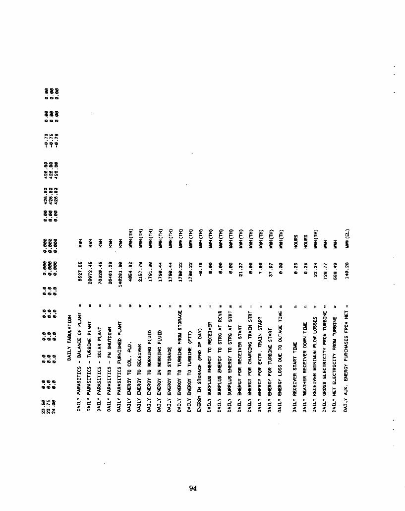
??? B B B
?Fs2. m m t NNN
94

rl t t B I- t- m la
B
n, 0 N I- m 0
3
x N la 4 la t rl
B
< \ z
U U W
B B
U 0
t t la rl
m 0 N IC
< \ z m
B
4
?
W V 4 K 0 I-
t
I- a 4
1y
E! t I- 94
N E! t c rl
B ? a
! B
t
N 01
n! la
B E!
la
B E! I
s; ! B ! B
II rl
V z U V K
V I
W z U m
I B B
II
II
U
v)
< I- v)
k rl
II n u II II II II I N n II H II II II II II I 1 I1
Y H I-
ll m I- K e v)
2 < K W Q 0
t- ? t 4 N
2 I-
I1 II It
8
k 4 K 0
K > V K
V K I- v) 5
J a.
v) w v) v) 0 J
s 0 J U
3 U
5 I K W > U W
2
P > J K
I- z < J a
K W > H g %
% H I-
W
I- 3
5 0
I- < I- < W V < I- 3 f a I-
4 8 n
Y H I-
g n
U 0 R 3 U
R 3 U
E e Z E
0 K I- v)
f 0 n
II W V
J T 2
n < I
W
I- z K
W > U W
K 8
z 0 U
< K I-
t;
a
K W > U W V W K
K < J 0 v)
0 I- V z : P
W V < E- v)
W z U
f 0 t-
x I
0 I-
O I-
J K
5 K W z i3 W K
K W > U
% W K
K W > U W U
a! a > 0 K W
3
I- K
v) 2
rl
J 0 U
0 I-
I I I I v) v) 0 J
v) V U
v)
4 0
CH d
v)
V U
in 4 K <
CH
n
v) V U
v)
<
L d a
v)
t- U
v) < K
Z
2
3 U
V K W z W
0 I-
z U 0 I- O
I- 8 3 a r V v)
II K W > U W
3 v)
3 f
K W E 5
v) > 4 0
v) > < n > V
f > V
I 8 V K 0 U
> V K x B
U 0 U 0
5 3 >
> J K < W
* J K
5 > J K
5 > J K < W >
5 K 4 W >
> J K
P > J K < W >
> J
3 >
95

B.2 Case 2: Modified SOLERGY Default Case
The second sample case models a liquid sodium external receiver connected to a two tank molten salt thermal storage system. In modeling a plant in which the receiver working fluid is different from the storage medium (1s = 3 in NMLSTRG) a charging heat exchanger is included (either tstcr # 0 andjor estcr # 0 in NMLSTRG). The turbine generator is capable of producing 100 MW,. The solar multiple of the system is 2.4, meaning that the heliostat field is capable of supply- ing the receiver with 2.4 times as much thermal power as is required to operate the turbine at its rated capacity. The thermal storage system is capable of op- erating the turbine for 12.35 hours at its rated capacity when the tank is fully charged. A sunfollowing dispatch strategy has been selected. meaning that the turbine will attempt to start electrical generation whenever power is being col- lected by the receiver.
The namelist input file (SOLNML.DAT) now defines this system, which is different from the default case in several major ways. This input namelist is:
$ NMLGEN $ END $ NMLLOC $ END $ NMLCOEF
fr = O., .276, .461, .559, -621, .636, .650, O., .274, .459, .556, .621, .636, .650, O., .268, .415. .549, .613, .632, .650, O., .306, .457, .546, .609, .630, .650, O., .258, .440, .537, .605, .628, .650, O., .292, .442, .533, .599, .624, .650. O., .295, .437, .528, .595, .621, .650
$ END $ NMLCOLF
$ END $ NMLRCVR
rs = 710., ereqd = 30., plxlr = 7 * 29.8
fs = 1186000.
$ END $ NMLPIPE $ END $ NMLSTRG
ptsmax = 720., pfsmax = 270., ptsmin = loo., pfsmin = 30.,
96

emax = 3275., clf = 0.14, 1s = 3, tstcr = 0.50, pwarmc = loo., pwarmd = 30.
$ END $ NMLTRBN
$ END $ DISPATCH $ END $ PRNTOUT
mflag = 0, ndaf = 1, ndal = 366
esmax2 = 3275.
$ END
The major changes in case 2 are in the collector field, receiver, and thermal storage system. The turbine generator remains identical to the default case, and therefore requires no further specification. All input values are echoed back in the SOLERGY output file SOLOUT.PRT, which is included on the next two pages. The output summary pages are given on the following two pages (mflag = 0) and are followed by a single day of detailed output (mflag = 4) for the first day of the year.
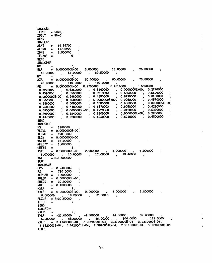
SNMLGW IFOUT = 50*0,
SEND SNMLLOC AUT = 34.89700 ALONG = 117.0220 , ZONE = 8.000000 a IFLAGP = 0 SEND
7, SNMLCOEF NX - ELR = 0.0000000E+00, 5.000000 15.00000 , 25.00000 ,
7, NY -
rsouT = 5o+o
-
45.00000 , 65.00000 , 89.50060 , - AZR = 0.0000000E+00, 30.00000 60.00000 , 75.00000 1
90.00000 11o.oooo 130.& FR = o . h ~ + o o , o.nisoooo 0.4~1oooO 0.559oooo 0.621oooO 0.6360000 , 0.6500060 , 0.OOOOObE+00, 0.274ooi)o , 0.4590000 , 0.5560000 I 0.621oooO , 0.6360000 , 0.6500000 0.0000000E+00, 0.2680000 , 0.415oooO , 0.5490000 I 0.613oooO I
0.632oooO , 0.6500000 , O.0000000E+OO1 0.3060000 , 0.457oooO ,
0.258ooOO , 0.4400000 0.537oooO 0.6050000 I 0.628oooO , 0.6500000 , 0.0000000€+00, 0.2920000 , 0.4420000 , 0.533oooO 0.599oooO , 0.624oooO I 0.6500000 , 0.0000000E+00, 0.2950000 , 0.437ooOO 0.528oooO , 0.5950000 , 0.621oooO , 0.6500000
0.546oooO , 0.6090000 1 0.6300000 1 0.65OOOOO 1 0.0000000E+W,
SEND SNMLCOLF FS = 1186000. 1
TLIML = 0.0000000E+00, TLIMU = 120.oooO ELM = 0.0000000E+00: WSLIM = 16.00000 , RFLCrY = 1.000000 , NEFWS = 81 WSX = 0.0000000E+00, 2.000000 4.000000 6.000000 , WSEF = 8+1.000000 SEND SNMLRCVR EPS = 0.948oooO , RS = 710.oooO ALPHAR = 1.000000 , TREQD = 0.0000000E+00, EREQD = 30.00000 RMF = 0.1OOOOOO , NXLR = 7, WXLR = O.OOOOOOOE+WI 2.000000 4.000000 , 6.000000 ,
PLXLR = 7*29.8oooO , IF ILL = 2 SEND SNMLPIPE NXLP = 9, TXLP = -22.00000 , -4.000000 14.00000 32.00000
YXLP = 3.4;3oOOOE-04 , 3.3629999E-04 , 3.3329999E-O4 , 3.2i19999E-04 , SEND
8.000000 , 10.00000 , 12,OOOb , 13.40060 ,
8.000000 , 10.00000 , 12.OOOb ,
50.00000 68.00000 86 .& 104 .d 122.0060 1
3.1520001E-04, 3.0710001E-04, 2.9910001E-04, 2.911-E-04, 2.8300000E-04
98

SNMLTRBN TBHWS = TBWCS = TPFSL = TMFS = ESMINl = ESMIN2 = ESMAXl = ESMAX2 = SDH - SDW = SDC RDH RDW RDC - NREPSS =
- - - - - - - -
12.00000 8
72.00000 , 265.oooO , 0.2500000 , 25.00000 25.00000 , 25.00000 3275.000 0.2000000 1
0.2400000 0.4000000 , 0.5500000 1.100000 8
3.33oooO ,
70.00000 80.00000 FEpSS 6+O.k98000 , 6+0:3992000 6+0.4148000 , 6+0.4183000 SEND SNMLSTRC PTSMAX = 720.oooO , PFSMAX = 270.oooO PTSMIN = 100.oooO , PFSMIN = 30.00000 , EMAX = 3275.000 , EMIN = 0.0000000E+00, ES = O.0000000E+W1 A = 3+0.0000000E+00, CLF = 0.1400000 , DLF = 0.1400000 , TNKLF = 0.1000000 LS - REFPC = 264.oooO TSTCR = 0.5000000 ESTCR = 0.0000000E+00, TSTDR = 0.2500000 , ESTDR = O.OOOOOOOE+OOl PWARMC = l00.oooO PWARMD = 30.00000 SEND $DISPATCH IDISP = 0 , TSTUR = 1.25oooO PSTFR = 0.5000000 I D F l = 400, IDF2 = 0 SEND SPRNTOUT MFLAC = 0 , NDAF = 1 1 NDAL = 366 SEND
3, -
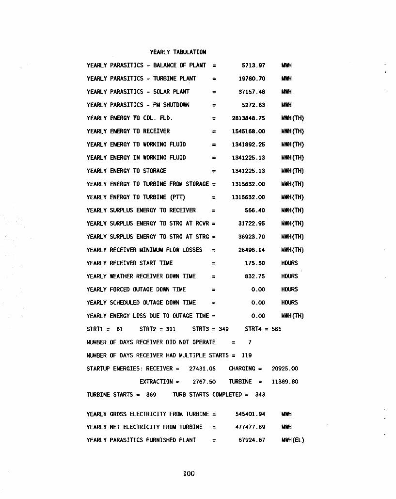
YEARLY TABULATION
YEARLY PARASITICS - BALANCE OF PLANT
YEARLY PARASITICS - TURBINE PLANT
YEARLY PARASITICS - SOLAR PLANT
YEARLY PARASITICS - PM SHUTDOWN YEARLY ENERGY TO COL. FLD.
YEARLY ENERGY TO RECEIVER
YEARLY ENERGY TO WORKING FLUID
YEARLY ENERGY I N WORKING FLUID
YEARLY ENERGY TO STORAGE
YEARLY ENERGY TO TURBINE FROM STORAGE =
- - YEARLY ENERGY TO TURBINE (Pl l)
YEARLY SURPLUS ENERGY TO RECEIVER
YEARLY SURPLUS ENERGY TO STRG AT RCVR =
YEARLY SURPLUS ENERGY TO STRG AT STRG =
YEARLY RECEIVER MINIMUM FLOW LOSSES =
YEARLY RECEIVER START TIME - YEARLY WEATHER RECEIVER DOWN TIME
YEARLY FORCED OUTAGE DOWN TIME - YEARLY SCHEDULED OUTAGE DOWN TIME
YEARLY ENERGY LOSS DUE TO OUTAGE TIME =
- -
- - - - - -
5713.97
19780.70
37157.48
5272.63
2813848.75
1545168 .OO
1341892.25
1341225.13
1341225.13
1315632.00
1315632 .OO
566.40
31722.95
36923.70
26496.14
175.50
832.75
0.00
0.00
0.00
STRTl = 61 STRT2 = 311 STRT3 = 349 STRT4 = 565
NUMBER OF DAYS RECEIVER D I D NOT OPERATE = 7
NUMBER OF DAYS RECEIVER HAD MULTIPLE STARTS = 119
STARTUP ENERGIES: RECEIVER = 27431.05 CHARGING = 20925.00
EXTRACTION = 2767.50 TURBINE = 11389.80
TURBINE STARTS = 369 TURB STARTS COMPLETED = 343
YEARLY GROSS ELECTRICITY FROM TURBINE = 545401 .94 MWH
YEARLY NET ELECTRICITY FROM TURBINE = 477477.69 MWH
YEARLY PARASITICS fXJRNISHED PLANT - - 67924.67 MWH (EL)
100

PLANT CHARACTERISTICS:
MAXIMUM POWER TO TURBINE = MAXIMUM POWER TO STORAGE = FIELD EFFICIENCY = 0,64429
= 0.906028 RECEIVER EFFICIENCY MAIN RECEIVER SIZE - STORAGE CAPACITY = 3275.OOMWhr TOTAL FIELD SIZE
265. OOMWT 720.ooMwT
710. OOMWT
= 1186000.OOSq M.
DESIGN POINT EFF.,ANNUAL EFF.
FIELD 0.64429450 0.57OO2121
RECEIVER 0.90602821 0.86844426
PIPING 0.99969941 0.99950284
THERMAL STORAGE N/A 0.98091811
WGS 0.41830003 0.41455507
OVERALL N/A 0.16968833

As in the previous example problem, the next six pages of output result from a case identical to the first case presented, except that only the first day has been run. Maximum output has been requested.
102

103

. . . . . . . . . . . . . . . . . . . . . . . . . . . . . . . . . . . . . . . . . . . . . . cccccccCccCcccccccccccCcccccccccccCCcccccccc N N N N N N N N N N N N N N N N N N N N N N N N N N N N N N N N N N N N N N N N N N N N
104

. . . . . . . . . . . . . . . . . . . . . . . . . . . . . . . . . B B B B B B B B B B B B Q B B B B B B B B B B B B B B B B Q B B B
. . . . . . . . . . . . . . . . . . . . . . . . . . . . . . . . . B B P B B B B B B B B B B B B B B B B B B O O Q B B B B B B B B B
. . . . . . . . . . . . . . . . . . . . . . . . . . . . . . . . . 8,
B B B B B B B B B B B B Q B B B B B B B B B B B B B B B B B B B B
. . . . . . . . . . . . . . . . . . . . . . . . . . . . . . . . . 4
B B B B B B B B B B B B Q B B B B B B B B B B B B B B B B B B B B
105
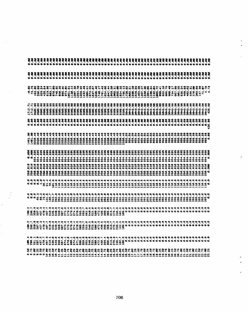
1 06

8 8 8
8 8 8 ???
8 8 8
IDIDm NNN 9tr
???
II II II II II If II I1 II II II II II I1
I-
Y I- K b
K
K 2 E
In ? ? ? 6 8 8 5
J O
z 0 H I-
3 4
I- > J n e a
W
I- ?I t
J L f
I- f d
E d t
I- < t K < t v)
x I
i!
a 0 LL
> W
>
< d a
3 O LL 0 e
3 U
e 3 LL
? ? ? 0 8 8 W
z H m
I I
8 2 X
J U W
t ?I
W z H W K
U 2
a < J 0 In I
K W
W
K
z Y
V E E P
0 I- W a K
I- a J < m
I O
I k f < ? ? ?
8 8 8
> 0 K W 3
J 0 U
0 I-
I K 0 LL
K 2 v)
U n k- H v) < K
2
v) U n
v) < K < O
t; 0 I-
O k-
z H K w
W U
Z
!+!
> V K W 3
> V
! > u K x
>
H ? ? ? 8 8 8
X
3 > J n 4 a
5 H 4 n
> J H 4 a
> J U
< a
> J n < n
> J H
< a
> J n < a
> J H
< a
> -I U < a
> > J J n u < < o n
> -I n < a
* < d a
> J n 4 a
> J U
< a J Y
< a
> J H < a m m r
NNN
107

N d
m d
I y! d
B
c (D (3
m a, W
B a?
r( (3 (A Q t a, a,
B ai
B t c 0 c m r(
Y B
OD Lo
OD N 4
Lo Lo d
B
U U W
U U W
a, 8, H (A 01 a, Lo
P (3
OD r(
B ?
d t (A 01
CD (A
01 a,
4 \ z
< \ z
B B B
W
K
v)
2 e
K w > H W
(r Y
J < P K W I I-
J J
W > 0
2 0 z H
l-4 P a
n J
U !!! 3 a
W
E H B
(3
OD
? !2
I1
n J U
-I 0 V
0 I-
t;
8 t -I
3 t
E z N
d d
d t
9
II
K w z Y L e t; 8 2 P
n I
E (3
N c Lo m
N
It
8 3 U
W z z P
1 m
N c Lo m
N
(I
t4
k
&
< K 0
0 I-
8 t -I K < W >
n I t z Lo
t
m
? 2
I1
W 0 < K 0 I- u)
I 0 K U
W z H m
2 e t;
5 z 3 t
H Lo
Lo d
y!
II
I- z < J
U 0
W V z <
I
In
n
3 m
x L v) 4 K < n
2 S t
c
m Lo N
I1
I-
-I
W z H
f a
I I
v) V H
v) 4 K <
t J
L;
a
3 t
d d
i d
I1
I-
-I
K
0 v)
I
v)
f
3 n
:: L
2
S
v) < K
2 t
d
y! t d
I1
f
1 E v)
I
I
u) V H
v) <
a
L;
s a t J K z
? * c ID (3
II
n H
U W z
3
e & 5 5 5
0 I-
3 t
d
I1 m I- K ti
d
II N
I- v)
z
H
11 d I- K I- v)
v)
!ii z 2 v)
W
H I-
I n *I 5 z W V W
v)
a
n 2 U 0
K
&! t
W I- < K W 0
I-
n
8 8
z n K W
W V W K
v)
2 n U 0
K
f 2
B
c 19
I1
5
d H I- V
k
II
W z U m
f P 0 K U
z
t, id
H V H K
W
v) v)
0 K W > -I K < W
II
W z H m
f
E z K U
V H
K I- V W J W
I- Y
s t J
W *
I1
I-
J f
s
I?
tH
a
I v) z v) V n
v) 4 0 <
t -I K < W t
a
II
F e I-
x 5 0 I-
* W K
x 3 t -I
t
I1
K W
> H W V W K
0 I-
G4
8
3 t
v)
a. K
3 v)
t J
3
II K
K
I- < W K I- v)
e
F t W
! 3 2 t -I K < F
I1
W K I- v)
I- < 0 K I- v)
0 I-
t W
8 v)
3
2
F
a K
* J K 4
I1
2 v) v) 0 J
% 0 J U
H 4 E
z Y
I K W
W K t J K
2
I t
W I U I-
I- K < I- v)
K W
W V 2 L
F
> J K <
I1
W
t- z 5 n
5 z Y L K W I I-
3 * J K < F
I 1
W
I- 5
5
2 2 8
0
W
I-
n
V (r
0 U
t J K
z
I1
Y H I-
5 n W W < I- 3 0
3 2 W I V v)
t J K < F
II
Y H I-
W W < t 3 0
0 t- W 3 n v) v) 0 J
t; 8 t J K
2
t
Lo W
?
II
K W > H W V L
E 8 3
v)
W
2 0 < ti
108

APPENDIX C: THE VALCALC PROGRAM
C. l The Value Calculator Post Processor Program
The VALCALC program calculates the net value of electricity generated by a power plant according to the avoided costs of The Southern California Edison Company (SCE) (15). Updates to this Standard Offer, including the most re- cent estimates of avoided costs, are described in the Avoided Cost Pricing Up- dates, which are published quarterly by SCE (16). These avoided costs are SCE’s marginal costs of generating electricity, and consist of costs for capital equipment and costs for fuel and variable operating and maintenance costs. The value of electricity is divided into capacity payment (s) and energy payments. The capac- ity payment is based on SCE’s avoided capital costs and is obtained either on a firm basis or on an as-available (also referred to as as-delivered) basis. The en- ergy payment is based on SCE’s avoided costs for fuel and for variable operating and maintenance costs. The rate periods, seasons, and holidays of SCE are de- fined by Schedule TOU-8 (6).
The avoided cost methodology is intended for use by a power producer exter- nal to the utility, such as a cogenerator or a small power producer. However, the value calculated by VALCALC can be interpreted as value to SCE, assuming that SCE would incur the same costs by generating the electricity itself. The following is a description the details of the avoided cost methodology, followed by a descrip- tion of its implementation in VALCALC.
The Avoided Cost Methodology of SCE
Energy Value
The energy value represents avoided operating costs and is based on a set of fixed rates for each rate period of each season per unit of electricity generated. Table C.l shows period energy value rates, used in VALCALC, that were effective in August 1985 (16).
The energy value is calculated as the electricity supplied to SCE multiplied by the energy value rate for the season and rate period during which the electricity was generated.

Table C.l. Period Energy Value Rates, y!/kWhr
On-peak Mid-peak Off-peak
Firm Capacity Value
Summer
6.1 4.7 4 .O
Winter
5.7 4.6 4 .O
To qualify for firm capacity payments under Standard Offer No. 2, a power producer must meet the Performance Requirement of SCE. This Performance Re- quirement requires that the power plant operate with a capacity factor of at least 80% during the on-peak periods of each of the summer months, June through September. The calculation of the monthly on-peak capacity factors is based on the Contract Capacity, the amount of electricity supplied to SCE during the period at power levels less than the Contract Capacity, and the duration of the period minus the amount of time during the period allocated for scheduled main- tenance. The Contract Capacity is the size of the plant in units of power. It may or may not be equal to the turbine power rating, and is used strictly to deter- mine firm capacity payments. Reasonable efforts must be made to perform regu- lar maintenance outside the months June through September. The firm capacity value of electricity is calculaded as follows:
Monthly Capacity Period Payment = (Contract Capacity Price)
* (Conversion From Annual to Monthly Payment)
* (Contract Capacity)
* (Period Performance Factor)
The Contract Capacity Price is determined by SCE for plants that begin op- eration at different times and operate for different lengths of time. The value of the Contract Capacity Price used in VALCALC is $88/kW-year, as obtained from The Avoided Cost Pricing Update (16) for a plant beginning operation in 1985 with a term of agreement of one year. The term of agreement specifies how long a plant will be obligated to provide electricity to SCE.
The conversion factors multiplying annual payment to give monthly payment are shown in Table C.2. These factors were obtained from the Avoided Cost Pric- ing Update (16). These factors increase the capacity payment during the on-peak period of the summer season relative to the capacity payment during other peri- ods.
.
110

Table C.2. Conversion to Monthly Payment
Summer Winter
On-peak Mid-peak Off-peak
0.1643 0.0028 0.0025
0.0245 0.0123 0.0036
The Contract Capacity is initially set equal to the net rated output of the turbine. In the event that the Performance Requirement is not satisfied, VALCALC decreases the Contract Capacity and repeats the value calculation in an attempt to meet the Performance Requirement at a lower value of the Con- tract Capacity. If the Performance Requirement cannot be satisfied and the Con- tract Capacity has been decreased to less than one-half of the net rated output of the turbine, then VALCALC calculates the capacity value based on the as- available capacity payment rates .
The Period Performance Factor is a capacity factor based on the net genera- tion at power levels less than the Contract Capacity and the duration of the pe- riod minus the time during the period allocated for scheduled maintenance.
Period Performance Factor =
Period net electricity generated [0.8 * (Contract Capacity) * (Period hours - Maintenance hours)]
The factor of 0.8 allows for a 20% forced outage rate in any month. The Pe- riod Performance Factor cannot exceed unity.
In addition to the Monthly Capacity Period Payment, a Bonus Payment may be earned during the summer months provided that the Performance Require- ment is satisfied and the on-peak capacity factor exceeds 85% for that month. During the winter months, as an additional requirement applying to the Bonus Payment, the on-peak capacity factor for each of the summer months must have exceeded 85%.
Monthly Bonus Payment = (1.2 * on-peak capacity factor - 1.02)
* (Contract Capacity Price)
* (1/12) * (Contract Capacity)

The on-peak capacity factor is calculated as follows:
On-peak capacity factor = . (Net generation during onpeak period)
(Contract Capacity) * (Period hours - Allowable Maintenance Hours)
As-Available Capacity Value
If the solar plant cannot satisfy the Performance Requirement for firm ca- pacity payments, then the capacity value is calculated based on the rates shown in Table C.3. These rates were obtained from The Avoided Cost Pricing Update (16).
Table C.3. As-Available Capacity Payment Rates, y!/k Whr
Summer Winter
On-peak Mid-peak Off-peak
10.95 0.13 0.05
2.62 0.58 0.07
The as-available capacity value is calculated as the net electric generation mul- tiplied by the as-available capacity payment rate for the season and rate period during which the electricity was generated.
The total value of electricity is equal to the sum of the energy value and ei- ther the firm capacity value or the as-available capacity value, minus the cost electricity for parasitics.
Cost of Electricity for Parasitics
VALCALC assumes that electricity required for plant parasitics are obtained from the gross electric generation of the plant. Parasitic power requirements in excess of the gross generation are obtained from SCE with cost (negative value) calculated according to Schedule TOU-8(6). The cost of electricity consists of a Customer Charge, a Demand Charge, and an Energy Charge. These charges are shown in Table C.4. The Demand Charge is calculated as the maximum power level at which SCE supplies electricity during each period of each month multi- plied by the Demand Charge Rate for that rate period.
112

Table C.4. Cost of Electricity
Customer Charge Rate
Demand Charge Rates On-peak Mid-peak Off-peak
Energy Charge Rates
On-peak Mid-peak 0 ff- peak
$ 560 per month
$ 5.05 per kW per month $ 0.65 per kW per month $ 0.00 per kW per month
8.426 # per kWhr 7.026 # per k Whr 5.856 per kWhr
Implementation of the Avoided Cost Methodology in VALCALC
VALCALC processes results from SOLERGY which are contained in the out- put file EGEN.DAT. Each record of EGEN.DAT contains values of gross electric generation, parasitic power required by the plant, and two flags signaling the oc- currence of outages. There is one record in the EGEN.DAT file for each time step of the simulation.
In VALCALC, the main program is a driver which:
(2.) Prompts the user for net turbine rating and time step duration;
(ii.) Calls the subroutine SCE; and
(ziz.) Prints the results to output file SUMMARY.DAT.
The subroutine SCE calls subroutine M’HEN, which determines the season, month, and rate period given the day of the year, the durat,ion of the time step, the local time at the end of the current time step, and two arrays specifying the beginning and ending times of each of the rate periods for each day of the year. These arrays are initialized in subroutine SCE and are for the calendar year 1984.
The subroutine SCE begins with an alphabet,ized list of variables, including their definitions and units. Then, the beginning and ending times of each of the rate periods are set in local time (not daylight savings time) for each day of the year. Next, the total time, the time for forced outages, and the time for scheduled maintenance during the year in each rate period for each month are calculated.
113

Capacity payment, energy payment, and cost rates for electricity are then set. The Contract Capacity is initially set equal to the net rated turbine output, and arrays of monthly period sums are set to zero.
For each time step of each day of the year, subroutine SCE determines the incremental electricity value or cost, and accumulates it in the appropriate ar- ray. At the end of the year, if the plant does not meet the SCE performance re- quirement for firm capacity (80% on-peak capacity factor for the summer months, June through September) then the algorithm reduces the Contract Capacity in an attempt to satisfy the performance requirement at a lower value of the Contract Capacity. This may not be possible, because the on-peak capacity factor is based on that amount of electricity generated at power levels less than the Contract Ca- pacity. As the Contract Capacity is decreased, the amount of electricity used to calculate the on-peak capacity factor may also decrease. Thus, a plant may not be able to qualify for firm capacity payments. If the plant does not qualify for the firm contract, then the as-available capacity payments are obtained.
The subroutine SCE then calculates sums and weighted averages for output by the main program.
The results from VALCALC are organized into eleven categories. For each of the categories, results are printed by month and by period. On-peak periods are designated by the integer 1, mid-peak periods by the integer 2, and off-peak periods by the integer 3. The following is a description of the categories:
1. Total time, hours
2. Maintenance time, hours
3. Forced outage time, hours
4. Gross electric generation, GWhr
5. Electrical parasitics, G Whr
6. Net, electric generation - gross electric generation minus electrical parasitics, GWhr
7. Capacity factor - the first four rows are capacity factor based on total pe- riod hours, net generation, and net rated turbine output. The fifth row is the on-peak capacity factor, as defined above. The numerator of the on-peak ca- pacity factor is gross electric generation for the period minus that portion of electrical parasitics obtained from gross electric generation. The last col- umn shows the average capacity factors weighted by the amount of time in each month, rather than an arithmetic average of the capacity factors for each month.
8. Total capacity value of the sum of the net electric generation and that portion of electrical parasitics obtained from SCE, million of dollars.
114

9. Total energy value of the sum of the net generation and that portion of elec- trical parasitics obtained from SCE, millions of dollars.
10. Charges - cost of electricity purchased from SCE for that portion of electrical parasitics obtained from SCE, millions of dollars.
11. Total net value - total capacity value plus total energy value minus charges, millions of dollars.
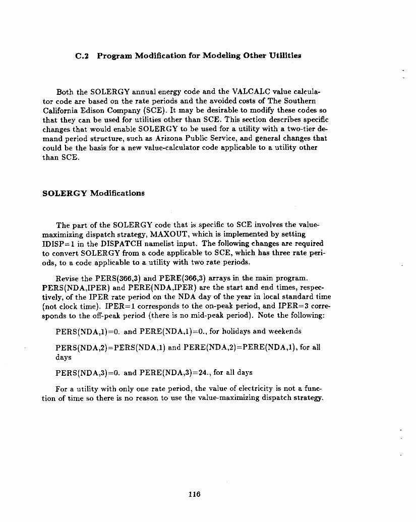
C.2 Program Modification for Modeling Other Utilities
Both the SOLERGY annual energy code and the VALCALC value calcula- tor code are based on the rate periods and the avoided costs of The Southern California Edison Company (SCE). It may be desirable to modify these codes so that they can be used for utilities other than SCE. This section describes specific changes that would enable SOLERGY to be used for a utility with a two-tier de- mand period structure, such as Arizona Public Service, and general changes that could be the basis for a new value-calculator code applicable to a utility other than SCE.
SOLERGY Modifications
The part of the SOLERGY code that is specific to SCE involves the value- maximizing dispatch strategy, MAXOUT, which is implemented by setting IDISP=l in the DISPATCH namelist input. The following changes are required to convert SOLERGY from a code applicable to SCE, which has three rate peri- ods, to a code applicable to a utility with two rate periods.
Revise the PERS(366,3) and PERE(366,3) arrays in the main program. PERS(NDA,IPER) and PERE(NDA,IPER) are the start and end times, respec- tively, of the IPER rate period on the NDA day of the year in local standard time (not clock time). IPER=l corresponds to the on-peak period, and IPER=3 corre- sponds to the off-peak period (there is no mid-peak period). Note the following:
PERS(NDA,l)=O. and PERE(NDA,l)=O., for holidays and weekends
PERS (ND A ,2) = PERS ( ND A, 1) and P ERE ( ND A ,2) = PERE (ND A, 1 ) , for all days
PERS(NDA,3)=0. and PERE(NDA,3)=24., for all days
For a utility with only one rate period, the value of electricity is not a func- tion of time so there is no reason to use the value-maximizing dispatch strategy.
116

VALCALC Modifications
The VALCALC code processes results from SOLERGY contained in the file EGEN.DAT. Since VALCALC is highly specific to SCE, for a different utility, an entirely new version of the program should be written, using VALCALC as a model. The following is a list of changes that would probably be required:
1. Revise the PERS(366,3) and PERE(366,3) arrays in subroutine SCE.
As in SOLERGY, PERS(NDA,IPER) and PERE(NDA,IPER) are the start and end times, respectively, of the IPER rate period on the NDA day of the year in local standard time (not daylight savings time). IPER=l corresponds to the on-peak period, and IPER=3 corresponds to the off-peak period (there is no mid-peak period). Note the following:
PERS(NDA,l)=O. and PERE(NDA,l)=O., for holidays and weekends
PERS (NDA,2)=PERS (ND A,1) and PERE( ND A,Z)=PERE(NDA,l), for all days
PERS(NDA,3)=0. and PERE(NDA,3)=24., for all days
2. Revise firm, bonus, and as-available capacity payment rates and calculation procedures, as required.
3. Revise energy payment rates and calculation procedures, as required.
4. R.evise electricity charge rates and calculation procedures for parasitics that are obtained from the utility, as required.
5. Revise the performance requirement for firm capacity payments, as required.

APPENDIX D: SAMPLE VALCALC PROBLEMS
Three example problems are presented to illustrate the results available from the program VALCALC. For the first example, VALCALC is used to analyze the results of the SOLERGY default case presented in Appendix B . l . The de- fault case uses the sunfollowing dispatch strategy, a solar multiple of 1.2, and 1.25 hours of thermal storage. The second SOLERGY case illust,rating VALCALC out- put is identical to the default case, except that: (i) the value-maximizing dispatch strategy is used and (22) the thermal storage capacity is increased from 1.25 hours to 4 hours. Finally, in the third example, VALCALC is used to analyze the re- sults of a SOLERGY case identical to the default case, except that: ( 2 ) the value- maximizing dispatch strategy is used and (22) the thermal storage capacity is in- creased from 1.25 hours to 6 hours. Thus, the second and third examples differ only in that the solar plant in the third example has two more hours of storage than that in the second example.
As described in Appendix C, VALCALC results include, on a monthly and annual basis, the following quantities for each period (on-peak = 1, mid-peak = 2, off-peak = 3):
1. Total t,ime, hours
2. Maintenance time, hours
3. Forced outage time, hours
4. Gross electric generation, G Wehr
5. Electrical parasitics, GU',hr
6. Net, electric generation, which is gross electric generation minus electrical par- asitics, GWehr
7 . Capacity factor: the first four rows are capacity factor based on total period hours, net generation, and net rated turbine output. The fifth row is the on- peak rapacity factor, as defined above. The numerator of the on-peak ca- pacity factor is gross electric generation for the period minus that portion of electrical parasitics obtained from gross electric generation. The last col- vmn shows the average capacity factors weighted by the amount of time in each month, rather than an arithmetic average of the capacity factors for each month.
8. Total capacity value of the sum of the net electric generation and that portion of electrical parasitics obtained from SCE, millions of dollars.

9. Total energy value of the sum of the net generation and that portion of elec- trical parasitics obtained from SCE, millions of dollars.
10. Charges: cost of electricity purchased from SCE for that portion of electrical parasitics obtained from SCE, millions of dollars.
11. Total net. value: total capacity value plus total energy value minus charges, millions of dollars.
VALCALC output also includes the total net value per unit of net electricity pro- duced by the plant.
D.l Case 1: Sunfollowing Dispatch
This case is a simulation of the default 100 MW, solar plant described in Ap- pendix B.l . The solar multiple of this plant is 1.2 and the storage capacity is 1.25 hours. A sunfollowing thermal energy dispatch strategy is used. Refer to Ap- pendix B.l for a description of this problem. SOLERGY results that are analyzed by VALCALC are contained in the file EGEN.DAT, which has one record for each time step of the simulation.
The VALCALC results for this case are shown on the next page. The results show that the plant generated 217.38 GWhr of net electrical energy and produced a net revenue of $14.292 million dollars for this year. The average value of the electricity produced was therefore 6.575 #/kWhr. As noted in the last line of VALCALC output, the capacity payments were determined by the as-available rates. The plant did not generate enough electricity during the on-peak periods of the summer to qualify for the greater firm-capacity payment rates. The difference between firm and as-available capacity payments is discussed in Appendix C.
120

d W
L
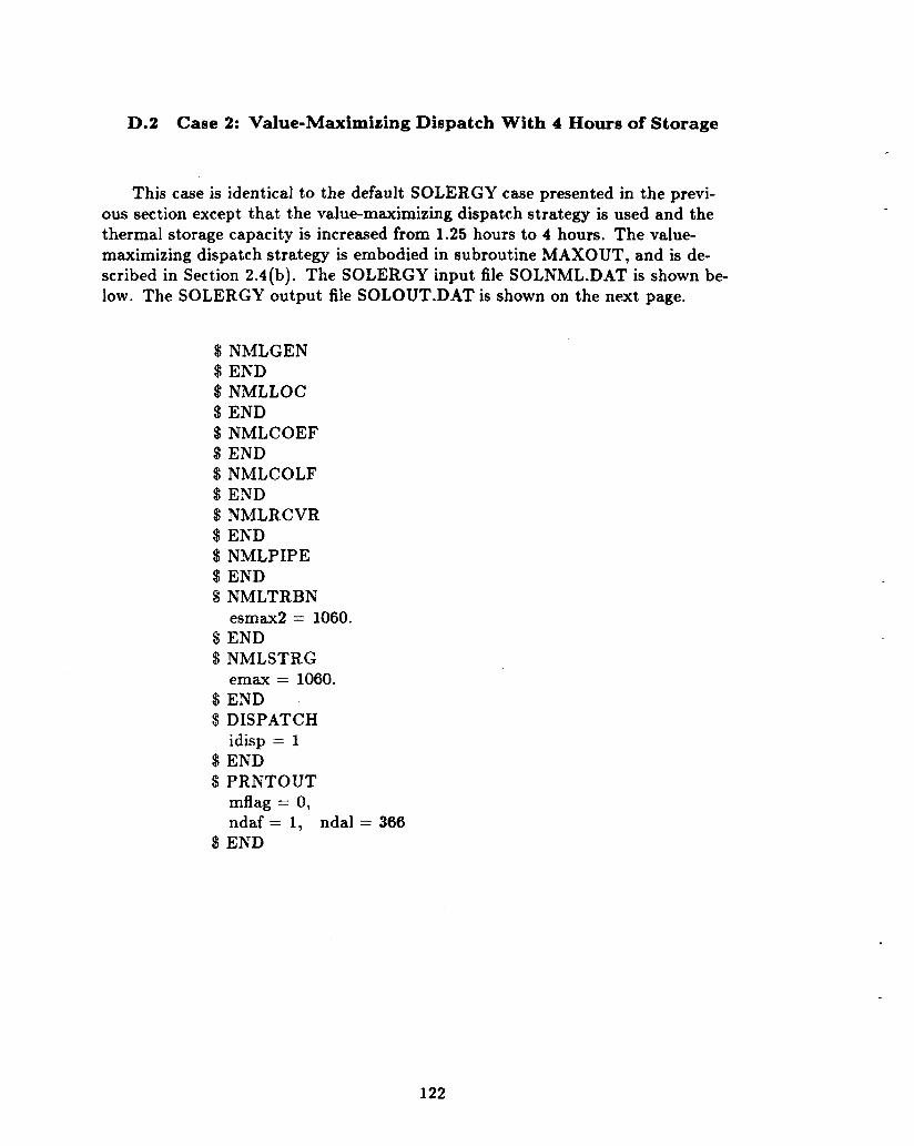
D.2 Case 2: Value-Maximicing Dispatch With 4 Hours of Storage
This case is identical to the default SOLERGY case presented in the previ- ous section except that the value-maximizing dispatch strategy is used and the thermal storage capacity is increased from 1.25 hours to 4 hours. The value- maximizing dispatch strategy is embodied in subroutine MAXOUT, and is de- scribed in Section 2.4(b). The SOLERGY input file SOLNML.DAT is shown be- low. The SOLERGY output file SOLOUT.DAT is shown on the next page.
$ NMLGEN $ END $ NMLLOC $ END $ NMLCOEF $ END $ NMLCOLF $ END $ NMLRCVR $ END !3 NMLPIPE $ END $ NMLTRBN
$ END $ NMLSTRG
$ END S DISPATCH
idisp = 1 $ END $ PRNTOUT
mflag = 0, ndaf = 1,
esmax2 = 1060.
emax = 1060.
ndal = 366 $ END
122
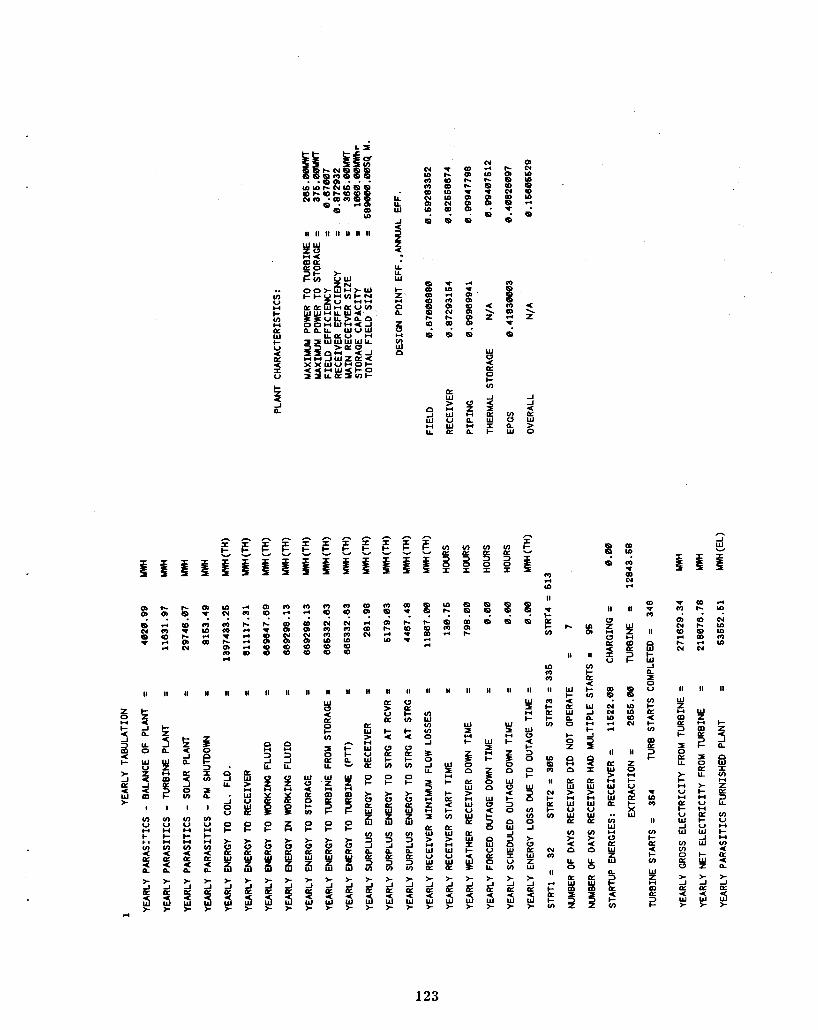
B U I- <
2 < I-
* J K
* 5
-4
E: h
0
s H m
-4
I1
I-
J
W
T
i5 a
$ I
v) U U
v) < K < > J K
L
n
2
E: I- ? s I- 0 N
II
I- z 5
5 a K
0 v)
I
v)
U U
v) 4 K < a.
> J
E
E 0
m W -4 OD
‘c
II
e 1 v)
x
I
v)
U U
v) < K < > J K
a
t,
n
2
E E W
m m t I- Q, m H
o!
II
!3 U
J 0 U
0 I-
> W K I 3 > J
>
4 u II I1 I1 II II II
i U L W
O W O - 4
f 2 I-
? B 9
I-
J n f
U
I U
W U W K 0 I- >
P > J K
2
II
R 3 L
0
B e 0 I-
> W K x > J K
> S
II
n U
U
W
3
i
P
e E > V
2 s >
II
W 0 < K 0
ti 0 I- * W K x 2 > J K
I1
3 4. K 0 I- v)
z K U
x 2
z 3
m
0 I- > W K
> J
>
II
E
f
a.
W z Y
U m
0 I-
> W K W 3 > J K
2
II
K W
W U W
z
e! a
> 0 K x v)
3 2
Y
n K
> J K <
I1
K > U K I- < 0 K I- v)
0 I-
>. W K W 3 3 2
v)
a K
> J K
2
II W K I- v)
2 0 K I- v)
0 + G K x v)
n K
3 2 > J K
< W >
II
v) W v)
v) 0 J
J U
4 U
E
s 6 g
I K W
a- J
K < W >
II
Y U I-
I- K < I- v)
K W
W V
z
> -I K < W >.
II
W I U
I-
5
z
0
PI W
W U W K K W I I-
a
s > J K < F
II
w I t U
5 0
W W <
n
2 a W U K 0 U > -1 K
z
II
W
I- I3
n W W < I- 3 0
W n
a s’ Y U v)
a- J
K < F
II W I U I-
w 0
< I- 3 0
0 I-
W 3
v) v) 0 A
> W K W
a
5 > J K
z
W
K W
0
I- O z
2 a
8
z g
n K W
W U
v) > <
U 0
K
n
I t
F K < I- v)
W J U I-
n
i 9
z I K W
W U W K v) * <
L 0
K W
n
m s
aD
N N W -4
-4
8.
II K W
W U
z g v) W U
0 K W
3 2 K < I- v)
9
W W (D N
8.
II
z I- U < K
s
i
n
U
v) I- K < I- v)
g
m
f
f W m
II v)
4 I- v)
W
k
E m
I
II
W E m
f I 0 K U
>. I- H
U U
K I- V W J W
v) v) 0 K 0
* J K
* 3
II
W z U m
f = 0 K U
a-
U U K
W 2 W
I- W z > J PI 4
W *
t,
t,
II
I- z < J n n W I v) H
z Q
3 U
v)
U c(
v) < (L <
> J PI 4
t,
a
F
123

The VALCALC results for this case are shown on the next page. The results show that the plant generated 218.08 GWhr of net electrical energy and pro- duced a net revenue of $16.699 million dollars. The average value of the electric- ity produced is therefore 7.657 #/kWhr. This is a significant improvement over the SOLERGY default case with the sunfollowing dispatch strategy. As noted in the last line of VALCALC output, the capacity payments were again determined by the as-available rates. Despite use of the value-maximizing dispatch strat- egy and an additional 2.75 hours of thermal storage, in July the plant could not generate enough electricity during the on-peak period to qualify for the greater firm-capacity payment rates. Recall that the performance requirement for firm capacity payments requires that the plant operate with an on-peak capacity fac- tor greater than 80% during the on-peak period for each summer month.
124

88.98 B B B Q c
V <
E 0
V W J m 5 s H <
v) <
K ti 8 .4
h 2)
V
V
2)
2)
0 U
c
a
K B
B ? f 2)
4 0
'0
4 K 2)
z
a n a
i x \
2) C
V
I. LO
I- ?
* a > 2)
z
m L
> <
-
i I 2
???? m m m t B B t t
.4 tc
???? B B B B
???? B B B B
???? B B B B
???? B B B B
B B B B
???? B B B B
???? B B B B
NQOC ? ? O D ? 2 m t m
N
$ * O D - .??? B d M t
m m c m e m d m ????
???? B B B B
???? B B B B
I - m c c
d L O a D L O F I N
'I???
88.8.8 B B B B
88.88. B B B B
U8I-r-m
t b t O F I N
?'I?'. Q t Q N
(ucDN.4 d N
?hi?? LOLOQNN
Q B c m Q ?"?? m m NYQD
NLONQ L O 4 L O . 4
B B B . 4 'I???
???? B B B B
? ? ? ? B B B B
???? W Q Q t NaDNt d 4 t C
???? t Q b B NmBN 4 4 t c
???? B B B B
???? B B B B
???? m m m t O D Q I 0 . C
d t t -
???? B B B B
? ? ? ? B B B B
???? 9 Q I - B
4 t h m m t c u
???? B B B B
? ? ? ? B B B B
m t m m
B B B B B
???? m m m t m m L O 9
d t I -
???? B B B B
$ $ $ $
???? B B B B
? ? ? ? B B B B
QOdLO (DNhcD (*N..lI-
B B B B . . . .
t m t . 4 QBNN
B B B B ? ? ? ?
???? B B B B
? ? ? ? B B B B
c t c m O D ? ? ?
t m t t N d I - d
V - t N t . . . .
.4
dN(n 4NO
2 3 3 - 0 I
E; C W 3 < K W
8
5" 3
z -E
- I C v) < o > -- >-
W z w
- 2: v)- 3: < o > .- > -
I-- W *- Z E -1
I- O I-
; e"
" r "
125
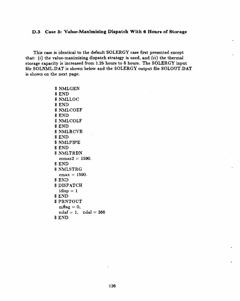
D.3 Case 3: Value-Maximizing Dispatch With 6 Hours of Storage
This case is identical to the default SOLERGY case first presented except that: (i) the value-maximizing dispatch strategy is used, and (ii) the thermal storage capacity is increased from 1.25 hours to 6 hours. The SOLERGY input file SOLNML.DAT is shown below and the SOLERGY output file SOLOUT.DAT is shown on the next page.
$ NMLGEN 8 END $ NMLLOC $ END $ NMLCOEF $ END $ NMLCOLF $ END $ NMLRCVR $ END $ NMLPIPE $ END $ NMLTRBN
$ END $ KMLSTRG
8 END $ DISPATCH
idisp = 1 $ END 8 PRNTOUT
mflag = 0, ndaf = 1,
esmax2 = 1590.
emax = 1590.
ndal = 366 $ END
126

B
t OD
n!
9
11
z J
U 0
W U
J 4.
I
v) U
a
f m
L
3
v) < K 4
> J
a
>
B Y 4 d
N d
r(
I1
I-
J
W z
f a
U
I I
v) U n L v) < K 4.
> J
a
3
B
t
0 N
? E
I1
I- z < J
K < J 0 v)
I
In U
a
n L
s v) 4.
a > J K < W >
E t
Lo t
?
%
II
f
1 0
I-
v)
I
I
v) U U
v) 4 K <
J
n
a
L
a
3 >
h I t E
n I t E
m m t c m d m
I1
n J U
-I 0 U
0 I-
> V K x > J K
< W >
OD
t d
OD
%
I1
K W > U
W K 0 I-
> 0
8
a x 2 > d
n I t E 8 l-
aD cy I- W
m
II
2 3 U
V z H
B
# 0 I-
> V
t J K
v)
U U I-
K W I- U
4. K < V
2
r I- z 3 a
j;. E (3 d
W t Lo
N l- W
I1
E? 3 U
W z z e E & K x 3 > J
>
i- ll ll ll ll ll ll ll
h I t ii
2 0 t Lo N c W
II
W V
0 I- v)
0 I-
>
2
I > -I K
2
h I t E
? m m OD W W
m
I1
W 0 4. K 0 I- v)
I 0 K U
W z U
I 0 I-
& K
8 > J K 4
F
U U W
H v) W n
B
t Lo d
m 0, cy c
B ?
d t 0 0
t < \ z
B
z z
8 4 K 0 I-
II
E e W z U
9
!i 0 t
z
> J
3 >
I1
K W z 8 W K
> V K x 3 a K 2 > J
I1
K > U K I- < 0 K
5l 0 t >
!!I
3 9 3 > J
I1
V K I- v)
I- < V K I- v)
0 I-
&
2 4 v)
v)
3
* -I K
2
I1
v) W v)
v) 0 J
g J U
U ; E I K W > U
W
> J
K <
Y a
e
127
I1
W I U I- I- K < t v)
K W > U W
E > J K < W >
II
W I U I-
5 0
K W >
n
9 W K
K W I
5 > J K
2
I1
W I U t-
f
8 2
3 8
0 n
< I-
n W
I V v)
> J
& 4 W >
I1
W L U
I- W 0 < I- 3 0
t W 3
v) v)
0 -I
> K
n
n
a
x > J K
< W >
In n, m I t
m L I- v)
In B m I1
r K I- In
01 m
I1 d
I- K I- v)
W
K W
0
I- O z
5 a
a n K W > U
Y g v) > 4
U 0
K
n
3 1
v)
c K
< I- v)
W J H I-
a
!i n < I
K W
W U W K
v) > <
U 0
K W
R
n
m s
l- d
(D
!5 r(
d
u K W > H W
K
v)
V K
$
!!
x 2 K 4 I- v)
B ? Lo N
I1
H
< K t X W
t,
-I a B r U
K 4. I- v)
m
f t t m
I1
v)
4 I- v)
W
t
E
I1
W z U
I I 0 K U
>
U U K I- V W J W v) v) 0
L
5 > J K
2
II
W z H
f I 0 K U
c
t;
Y
U U U K
W J W I-
> J K
< W t
I1
I- z 4 J a
8
i?
k
I
i v) U U
v) < K 4
> -1 K
< W >
a

The VALCALC results for this case are shown on the next page. The results show that the plant generated 220.87 GWhr of net electrical energy and produced a net revenue of $18.705 million dollars. The average value of the electricity pro- duced was therefore 8.469 #/kWhr. This is a significant improvement compared to both the default, SOLERGY case and the case with four hours of storage. As noted in the last line of VALCALC output, the capacity payments were deter- mined by the firm capacity payment rates. The Contract Capacity for the firm contract was the net rated output of the turbine, 100 MW,.
128

d N O r ( N 0 4 N O 0 - a > I
3' I- z n < I
E ; I-V I i V
f 9 2 2 <
- c- We- Z E
> V K W J 0 ul
n W V
LL 5
E J < E
1291 130

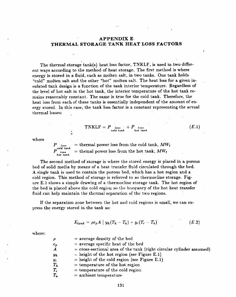
APPENDIX E THERMAL STORAGE TANK HEAT LOSS FACTORS
The thermal storage tank(s) heat loss factor, TNKLF, is used in two differ- ent ways according to the method of heat storage. The first method is where energy is stored in a fluid, such as molten salt, in two tanks. One tank holds “cold” molten salt and the other “ h ~ t ” molten salt. The heat loss for a given in- sulated tank design is a function of the tank interior temperature. Regardless of the level of hot salt in the hot tank, the interior temperature of the hot tank re- mains reasonably constant. The same is true for the cold tank. Therefore, the heat loss from each of these tanks is essentially independent of the amount of en- ergy stored. In this case, the tank loss factor is a constant representing the actual thermal losses:
TNKLF = P i o r s + P 10.8
cold tank hot tank t ++
where P l o r r
P‘d~:p”k = themal power loss from the hot tank, MWt = thermal power loss from the cold tank, MWt
hot tank
The second method of storage is where the stored energy is placed in a porous bed of solid media by means of a heat transfer fluid circulated through the bed. .4 single tank is used to contain the porous bed, which has a hot region and a cold region. This method of storage is referred to as thermocline storage. Fig- ure E.l shows a simple drawing of a thermocline storage tank. The hot region of the bed is placed above the cold region so the buoyancy of the hot heat transfer fluid can help maintain the thermal separation of the two regions.
If the separation zone between the hot and cold regions is small, we can ex- press the energy stored in the tank as:
where: average density of the bed average specific heat of the bed cross-sectional area of the tank (right circular cylinder assumed) height of the hot region (see Figure E.1) height of the cold region (see Figure E.l) temperature of the hot region temperature of the cold region ambient temperature
131

'h
Figure E-1. Thermocline Storage Tank
L
132

The average temperature of the tank, Taue, is
where L is the total height of the bed. The heat loss rate of the tank, Piodd, can be expressed in terms of the average tank temperature and the thermal resis- tance, R, of the tank insulation:
Equation (E.2) can be rearranged into the following form:
The first two terms on the righthand side of Equation (E.5), when compared to Equation (E.3), are equal to LT,,,, and the sum ( y h + y c ) is equal to L. Therefore, we have
which can be inserted into Equation (E.4) to produce the following relationship between the amount of stored energy and the heat loss rate:
Etank pcpALR PlOSd =
This relationship for the heat loss from a thermocline storage tank differs from that for two-tank storage in two very important ways:
1.
2.
The heat loss rate for thermocline storage is a funct.ion of the level of charge whereas for two-tank storage it is independent of the level of charge.
The energy stored in the thermocline storage tank must be expressed as an energy relative to the ambient temperature whereas the energies in a two- tank storage system can be referenced to the cold tank temperature as is com- monly done.

The tank loss factor for a thermocline storage system is a constant equal to the denominator of Equation (E.7):
TNKLF = pc,ARL
If the heat losses from the thermocline storage tank are specified to be a frac- tion, f, of the maximum available stored energy (EMAX - EMIN) in a time pe- riod At , then the following is true:
f(EMAX - EMIN) - EMAX - At pc,ALR plods =
which can be rearranged to determine the tank heat loss factor:
At EMAX TNKLF = pcpALR = - f EMAX - EMIN
134

References
I11
PI
PI
j4j
j 51
161
i 71
181
j9]
1101
ill]
Woodard, J. B. and G. J. Miller, “STEAEC - Solar Thermal Electric Annual Energy Calculator Documentation,” Sandia National Laboratories report, SAND77-8278, January 1978.
Falcone, P. K., “A Handbook for Solar Central Receiver Design,” Sandia Na- tional Laboratories report, SAND86-8009, December 1986.
Kistler, B. L., “A User’s Manual for DELSOL3: A Computer Code for Calcu- lating the Optical Performance and Optimal System Design for Solar Thermal Central Receiver Plants,” Sandia National Laboratories report, SAND86-8018, November 1986.
Leary, P. and J. D. Hankins, “User’s Guide for MIRVAL - A Computer Code for Comparing Designs of Heliostat-Receiver Optics for Central Receiver Solar Power Plants,” Sandia National Laboratories report, SAND77-8280, February 1979.
Haskell, K. H. and W. H. Vandevender, “Brief Instructions for Using the San- dia Mathematical Subroutine Library (Version 8.0) ,” Sandia National Labora- tories report, SAND77-1441, July 1980.
Southern California Edison Co., “Schedule No. TOU-8 General Service - Large,” Effective May 21, 1985.
Chiang, C. J., “SUNBURN: A Computer Program for Evaluating the Poten- tial of Solar Central Receiver Electric Power Plants,” Sandia National Labora- tories report, SAXD86-2165, February 1987.
Norris, H. F., “Utilizing Spreadsheets for Analyzing Solar Thermal Cen- tral Receiver Power Plant Designs,” Sandia National Laboratories report, SAND86-8011, July 1986.
“Molten Salt Electric Experiment Steam Generator Subsystem Final Report,” cont,ractor report prepared by Babcock & Wilcox Nuclear Division, SAND85-8181, April 1986.
“Electric Power Generating Subsystem Study for Advanced Water/Steam Receivers,” Final Technical Report (Draft), February 12, 1980, prepared for Sandia National Laboratories by General Electric Company, contract 83-7550.
Baumeister, T, et. al., Marks’ Standard Handbook for Mechanical Engineers, Eighth Edition, McGraw-Hill Book Company, New York, NY, 1978.
135

[ 121 Walraven, R. “Calculating the Position of the Sun,” Solar Energy, Vol. 20, No. 5-C, pp. 393-397, November 1978.
[ 13j Zimmerman, J. C. “Sun-Pointing Programs and Their Accuracy,” Sandia Na- tional Laboratories report, SAND81-0761, May 1981.
1141 Kreider, J. F. and F. Kreith, Solar Energy Handbook, McGraw-Hill, 1981.
[ 151 Southern California Edison Co., “SCE Standard Agreement Firm Power Purchase,” Document No. 1895H, Effective February 14, 1983, revised August 19, 1985.
I161 Southern California Edison Co., “Avoided Cost Pricing Update for Cogenera- tion and Small Power Producers,” August 1985.
136

MAY 5, 1987 UNLIMITED RELEASE INITIAL DISTRIBUTION
U.S. Department of Energy (5) Forrestal Building Code CE-314 1000 Independence Avenue, S. W. Washington, D.C. 20585 Attn: H. Coleman
S. Gronich F. Morse M. Scheve R. Shivers
U.S. Department of Energy Forrestal Building, Room 5H021C Code CE-33 1000 Independence Avenue, S.W. Washington, D.C. 20585 Attn: C. Carwile
U. S. Department of Energy P.O. Box 5400 Albuquerque, NM 871 15 Attn: D. Graves
U.S. Department of Energy 1333 Broadway Oakland, CA 94612 Attn: R. Hughey
University of California Environmental Science and Engineering Los Angeles, CA 90024 Attn: R. G. Lindberg
University of Houston (2) Solar Energy Laboratory 4800 Calhoun Houston: TX 77704 Attn: A. F. Hildebrandt
L. Vant-Hull
University of Kentucky Dept. of Chemical Engineering Lexington, KY 40506 Attn: J. E. Funk
University of Utah Mechanical & Ind. Engineering Dept. Salt Lake City, Utah 84112 Attn: R. F. Boehm
137

Analysis Review and Critique 6503 81st Street Cabin John, MD 20818 Attn: Carlo La Porta.
Arizona Public Service Company P.O. Box 21666 Phoenix, AZ 85036 Attn: E. Weber
Babcock and Wilcox (2) 91 Stirling Avenue Barberton, OH 44203 Attn: D. C. Smith
D. Young
Battelle Pacific Northwest Laboratories (5) Battelle Boulevard Richland, WA 99352 Attn: J . A. Dirks
Bechtel Group, Inc. (4) P. 0. Box 3965 San Francisco, CA 94119 Attn: P. DeLaquil
S. Fleming B. D. Kelly S. Pate1
Black & Veatch Consulting Engineers (2) P.O. Box 8405 Kansas City, MO 64114 Attn: J . C. Grosskreutz
J . E. Harder
Black & Veatch Consulting Engineers (2) 11401 Lamar Ave. Overland Park, KS 66214 Attn: J . Arroyo
L. E. Stoddard
Boeing Aerospace Mailstop JA-83 P. 0. Box 1470 Huntsville, AL 35807 Attn: W. D. Beverly
California Energy Commission 1516 Ninth St., M/S 40 Sacramento, CA 95814 Attn: A. Jenkins
138

California Public Utilities Com. Resource Branch, Room 5198 455 Golden Gate Ave. San Francisco, CA 94102 Attn: T. Thompson
Cent.ro Investigations Energetica Medroansental Technologie (CIEMAT) Avda. Complutense, 22 28040 Madrid Spain Attn: F. Sanchez
DFVLR EN-TT Institute for Technical Thermodynamics Pfaffenwaldring 38-40 7000 Stuttgart 80 Federal Republic of Germany Attn: Dr. Manfred Becker
El Paso Electric Company P.O. Box 982 El Paso, TX 79946 Attn: J. E. Brown
Electric Power Research Institute (2) P.O. Box 10412 Palo Alto, CA 94303 Attn: J. Bigger
E. DeMeo
Foster Wheeler Development Corp. (3) 12 Peach Tree Hill Road Livingston, NJ 07039 Attn: T. V. Narayanan
S. F. Wu R. J. Zoschak
Georgia Institute of Technology GTRI/EMSL Solar Site Atlanta, GA 30332
D. Gorman 5031 W. Red Rock Drive Larkspur, CO 80118
Jet Propulsion Laboratory 4800 Oak Grove Drive Pasadena, CA 91103 Attn: M. Alper

Los Angeles Department of Water and Power Alternate Energy Systems Room 661A 111 North Hope St. Los Angeles, CA 90051 Attn: Hung Ben Chu
Martin Marietta Aerospace P.O. Box 179, MS LO450 Denver, CO 80201 Attn: T. Buna
h4cDonnell Douglas (4)
5301 Bolsa Avenue Huntington Beach, CA 92647 Attn: D. Barron
R. L. Gervais J. E. Raetz S. Saloff
MS 49-2
Meridian Corporation 5113 Leesburg Pike Falls Church, VA 22041 Attn: D. Kumar
New Mexico Public Service (2) M/S 0160 Alvarado Square Albuquerque, NM 87158 Attn: T. Ussery
A. Martinez
Olin Chemicals Group (2) 120 Long Ridge Road Stamford, CT 06904 Att,n: J. Floyd
D. A. Csejka
Pacific Gas and Electric Company 77 Beale Street San Francisco, CA 94106 Attn: J. Laszlo
Pacific Gas and Electric Company (4) 3400 Crow Canyon Road San Ramon, CA 94526 Attn: G. Braun
T. Hillesland, Jr. B. Norris C. Weinberg
140

Public Service Company of Colorado System Planning 5909 E. 38th Avenue Denver, CO 80207 Attn: D. Smit,h
Resource Analysis P. 0. Box 91890 Los Angeles, CA 90009 Attn: S. Roseman
Rockwell International Rocketdyne Division 6633 Canoga Avenue Canoga Park, CA 91304 At,tn: J. Friefeld
Sandia Solar One Office P. 0. Box 366 Daggett, CA 92327 Attn: A. Snedeker
Science Applications International Corp. (2) 10401 Roselle Street San Diego, CA 92121 Attn: K. Beninga
B. Butler
Solar Energy Research Institute (4) 1617 Cole Boulevard Golden, CO 80401 Attn: B. Gupta
J. Anderson D. Hawkins K. Weaver
Solar Kinetics Inc. P.O. Box 47045 Dallas, TX 75247 Attm: J. A. Hutchison
Solar Power Engineering Co., Inc. (2) P.O. Box 91 Morrison, CO 80465 Attn: H. C. Wroton
M. Connolly
Southern California Edison P.O. Box 325 Daggett, CA 92327 Attn: C. Lopez

Southern California Edison (2) P.O. Box 800 Rosemead, CA 92807 Attn: J. E. Reeves
P. Skvarna
Stlearns Catalytic Corp. P.O. Box 5888 Denver! CO 80217 -4ttn: T. E. Olson
Stone and Webster Engineering Corporation P.O. Box 1214 Boston, MA 0210; Attn: R. W. Kuhr
6000 6220 6221 622 1 6222 6222 6222 6222 6226 6226 6226 6226 6227 6227 8000
8100
8130 8131 8131 8133 8133 8133 8133 8242 8243 8244 8245 8400
8434 8434 8435 8265
D. L. Hartley; Attn: D. G. Schueler E. C. Boes C. J. Chiang (5) K. R. Boldt W. A. Couch C. R. Maxwell J. V. Otts D. J. Alpert J. T. Holmes (25) G. J. Kolb C. E. Tyner J. M. Diggs H. E. Reilly R. S. Claassen; Attn:
E. E. Ives; Attn:
V. Dugan, 6200
R. J . Detry, 8200 P. Mattern, 8300
J. B. Wright, 8150 D. J. Bohrer, 8160 R. A. Baroody, 8180
J. D. Giison S. E. Faas (5) H. M. Witek A. F. Baker Secretary, send to NESC (20) A. C. Skinrood (5) D. N. Tanner B. L. Kistler D. B. Dawson C. Hartwig R. J. Kee R. C. Wayne, Attn:
M. C. Stoddard (5) J. B. Woodard P. K. Faicone Publications Division for OSTI (30)
J. Vitko, 8430 H. Hanser, 8440
142

8265 Publications/Technical Library Processes, 3141 3141 Technical Library Processes Division (3) 8024-2 Central Technical Files (3)
143


![APPENDIX A MATLAB CODE FOR CALCULATION OF MOTOR …researchrepository.murdoch.edu.au/4117/4/Cho_2010_Appendiices.pdf · Table 1 MATLAB code for calculating motor torque[1] ... Motor](https://static.fdocuments.net/doc/165x107/5aa6f2ff7f8b9a424f8bae52/appendix-a-matlab-code-for-calculation-of-motor-1-matlab-code-for-calculating.jpg)