Solar Valuation: An Appraiser's Guide to Solar

Sunlight hits the solar panels and electricity exits

DC power is converted to AC power for household use

Excess power goes to the grid for credit

1.

2.3.

1.

2.

3.

How Solar Works

This guide is an introductory overview for residential real estate appraisers on how to accurately valuate a residential rooftop solar electric (PV) system.

Solar Valuation An Appraiser’s Guide to Solar

Summary How much is solar worth?Because using electricity is not an option, a solar system should not be treated like other amenities in a home. A solar electric system has a uniquely quantifiable benefit: electricity that powers the home. A solar electric system can significantly reduce the cost of ownership. These saved costs should be valued with the home (and the mortgage). In addition, rising utility rates mean that savings, or avoided costs, will increase in the future. Thus, purchasing a rooftop solar system is an economic home-investment. Recent studies show that a solar system increases the property value by a substantial amount, often recovering 100% of the original cost. It is therefore important to give the solar system an accurate value. This may not always be easy to do, especially since solar homes are still relatively new in the real estate market.

Contents• Solar & How it Works• Electricity 101• Solar Economics• Market Valuation Studies• Calculator Tools

©2012 SunPower CorporationPV Value is a registered trademark of Sandia National Lab and Solar Power Electric. All rights reserved.

Valuable Studies•Appraisal Journal Study•Berkeley Lab Report•Premier Gardens Case Study•Ryness Absorption Study•Seattle & Portland Metro Area Study

CalculatorsThere are free tools—provided by state and federal governments—to help you accurately calculate the value of a PV rooftop solar system.

Sandia and Solar Power Electric offer the PV Value™ tool:http://energy.sandia.gov/?page_id=8047

NREL offers the PVWatts™ calculator:http://www.nrel.gov/rredc/pvwatts/

Read on for more detailed information.

Solar systems are measured in DC kW (kilowatts).

Roughly 1 kW = 1,500 kWh/year

2

The Panels & InverterThe solar electric system—also called a PV or photovoltaic system—produces electricity for in-home consumption. The solar system turns on automatically in the morning and turns off automatically at night. From sunrise to sunset, the system converts sunlight into electricity. Solar cells within the panels produce direct current (DC) electricity that flows into an inverter typically located on the inside wall of the garage. The inverter converts DC electricity into alternating current (AC), which is required for residential use to power appliances and fixtures, and instantly delivers the converted electricity to the home’s electric service panel.

How Solar Works

Grid-Connected Solar Systems The electric service panel first uses the solar electricity to supply all of the power required by the home. When the solar system generates more energy than the home consumes, surplus electricity travels through the meter and into the local power grid. The electric meter spins backward and the electric bill decreases (known as “net metering”).

Over the course of the month, if the solar system produces more electricity than the home consumes, the electric bill will be credited for the surplus electricity. Homeowners will be credited at the same rate as if they had purchased the electricity from their local utility.

Solar Electric SystemNot all solar cells are the same. There is a wide range of efficiency and performance based on the cells used to make the solar panel. Solar electric systems constructed of high-efficiency cells, modules, and inverters will generate more power and thereby delivery greater financial benefits.

Life Expectancy of a Solar SystemMost solar systems today come with a 20 or 25-year warranty for power performance. Expected useful life is likely to be 40 to 50 years. The best evidence we have for expected useful life is the existence of several hundred systems that were installed 30 to 40 years ago and still operate today. With the technological advancements made in performance and reliability, it would be safe to assume that today’s systems would last at least as long. In general, solar systems are expected to last 30 years or more if the modules and inverters are qualified and certified products, installation and testing was properly done, and the system is well maintained (inverter replaced after 12-18 years, production monitoring is continued, and the panels are kept clean from excessive dust and debris).

What’s the science behind the solar panel?A solar panel is made up of a number of photovoltaic cells. Photovoltaic (PV) is a method of generating electricity by converting solar energy into direct (DC) current. The PV cells are generally made from thin wafers of silicon, the second most abundant substance on Earth—the same substance that makes up sand. To make the wafers, the silicon is heated to extreme temperatures, and chemicals, usually boron and phosphorous, are added. The addition of these chemicals makes the silicon atoms unstable (their electrons become less tightly held). When photons of sunlight hit a solar panel, some are absorbed into the solar cells, where their energy knocks loose some of the modified silicon's electrons. These loose electrons flow to wires that have been placed within the cells. This flow of electrons through the wires is electricity, which flows to the inverter for conversion to AC power.

Inverter An electrical device that converts direct current (DC)

to alternating current (AC).

Photovoltaic Cell Thin squares, discs, or films of

semiconductor material that generate voltage and current

when exposed to sunlight.

Panel or Module Photovoltaic cells wired together and laminated

between glass (on top) and an encapsulant (on bottom).

Array or System One or more panels wired together at a specific voltage, installed or mounted with

attaching hardware.

A home with an electric solar system is like a car that makes its own gasoline.

3

Electricity 101

= 1,000 watts = 1 kilowatt

So how much solar will a system produce? Solar system sizes are measured in kW (kilowatts). A 1 kW solar system will produce roughly 1,500 kWh (kilowatt-hours) per year.

Electricity MeasurementElectricity is measured in kilowatt-hours. A watt is a unit of power that measures the rate of energy conversion. A typical household incandescent light bulb uses electrical energy at a rate of 25 to 100 watts.

A typical household incandescent light bulb uses electrical energy at a rate of 25 to 100 watts.

Ten 100-watt bulbs are equal to 1,000 watts, which is equal to 1 kilowatt. A kilowatt-hour is a measure of how many kilowatts are being used in one hour. If you turn on those ten bulbs for one hour, that would equal one kilowatt-hour.

Tier 11-376 kWh

$0.11

Tier 2377-489 kWh

$0.13

Tier 3490-752 kwH

$0.25

Tier 4753-1128 kWh

$0.28

Tier 51129+ kWh

$0.29

Table1-Avg.tierrates&baselinesofCAinvestor-ownedutilities(May2012)

Baseline

$41

$27

Tier 2

$15

$0

Tier 3

$18

$0

Tier 4

$0

$0

Cost

without solar $74

with solar $27

Average monthly consumption

Average monthly solar production (2.5 kW)

Remainder purchased from Utility

kWh

562

313

249

Table2-AverageCAhouseholdenergybill(brokendownintiers)

Electricity ConsumptionHow many kilowatt-hours do you think most families consume each month? This is actually a very difficult question to answer because people live such different lifestyles. A large family with several big-screen televisions, computer equipment, and a pool or spa will use much more energy compared to a family with fewer of those items. Also, everyone’s home is different, and some are more energy efficient than others.

The U.S. Energy Information Administration (EIA) 2010 census for the US average residential electricity use per household is 958 kWh per month (or 11,496 kWh per year). [Source: “Residential Average Monthly Bill by Census Division, and State 2010.” EIA. 3 November 2011. Web. 11 May 2012.] Every utility is different, but many charge for power using a tiered system, where everyone starts out buying electricity at a baseline rate at the beginning of the billing cycle. Once a home goes over the baseline, homeowners move into a higher tier with a higher rate. High energy users can get up to the highest tier, which, in Table 1, is $0.29 per kilowatt hour.

For demonstration purposes, we will use the consumption pattern for the average California household which uses 567 kilowatt hours per month; their electricity bill would be $74. They went up to Tier 3 charges [Table 2].

If this family were to install a 2.5 kilowatt system on their home, producing an average of 313 kilowatt hours per month, they could get their bill down to as low as $27 a month. They could opt to buy a larger solar system and wipe out their bill altogether, but it’s not always the best financial choice, because a larger system may be more than what it costs to buy power at the baseline rate.

Rule of Thumb:1 kW = 1,500 kWh/yr

Electricity savings with solar: Monthly savings $47

Annual savings $564

Lifetime savings $23,488** Based on annual savings of $564 over 25 years with an estimated 4% electricity rate increase per year.

4

Lower Ownership Cost

Compared with standard homes, energy-efficient solar homes use substantially less energy for heating, cooling, and water heating. That’s a savings of almost $140 a month. Over the lifetime of the system, the homeowner can save more than $80,0002! Financing the home purchase using an energy efficient mortgage could lead to even greater savings.

1See www.eia.gov/electricity/data.cfm#sales for more information on electricity usage and rates.2 Based on home in San Diego, CA, with $150 per month electric bill. System financed with 25-yr home loan at 3% interest.3 Nevin, Bender, & Gazan. October 1999. “More Evidence of Rational Market Values for Home Energy Efficiency.” The Appraisal Journal, 67 (454-60). 4 Lawrence Berkeley National Laboratory (2011). Analysis of the Effects of Residential Photovoltaic Energy Systems on Home Sales Prices in California. April 2011. Berkeley: Berkeley Lab, Report LBNL-4476E.

Berkeley Lab Report: An Analysis of the Effects of Residential Photovoltaic Energy Systems on Home Sales Prices in California

In a more recent study, Berkeley Lab analyzed nearly 72,000 homes that resold, with 2,000 of these homes including solar.4 The research found that the solar homes sold for an average home sales price premium of approximately $17,000 for a relatively new 3.1 kW PV system (the average size of PV systems in the Berkeley Lab dataset), or $5.5/watt (DC). When expressed as a ratio, an average California home with PV installed equates to a 14:1 to 22:1 sale price to energy savings ratio respectively. This is comparable to the investment that homeowners have made to install PV systems in California (after applicable state and federal incentives).

Saving Money

As utility companies continue to raise their rates, the solar system can keep energy bills low. Nationally, utilities have increased electricity rates an average of about 3-6% per year for the last 30 years1. These rates will only continue to increase. With a solar home, homeowners can lock in lower rates for their solar electricity, and purchase less power from the utility. While the cost of electricity increases with time, the cost of home solar power remains low and constant.

Increasing Property ValueThe Appraisal Journal: More Evidence of Rational Market Values for Home Energy Efficiency

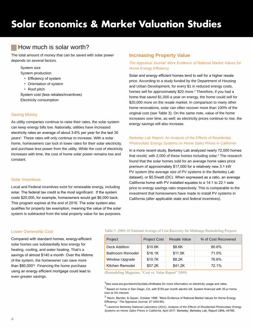
Solar and energy efficient homes tend to sell for a higher resale price. According to a study funded by the Department of Housing and Urban Development, for every $1 in reduced energy costs, homes sell for approximately $20 more.3 Therefore, if you had a home that saved $1,000 a year on energy, the home could sell for $20,000 more on the resale market. In comparison to many other home renovations, solar can often recover more than 100% of the original cost (see Table 3). On the same note, value of the home increases over time, as well; as electricity prices continue to rise, the energy savings will also increase.

Project Project Cost Resale Value % of Cost Recovered

Deck Addition $10.6K $8.6K 80.6%

Bathroom Remodel $16.1K $11.5K 71.0%

Window Upgrade $10.7K $8.2K 76.6%

Kitchen Remodel $57.2K $41.2K 72.1%

(RemodelingMagazine,“Costvs.ValueReport”2009)

Table3:2009-10NationalAverageofCostRecoveryforMidrangeRemodelingProjects

Solar Economics & Market Valuation Studies

How much is solar worth? The total amount of money that can be saved with solar power depends on several factors.

System sizeSystem production

• Efficiency of system• Orientation of system• Roof pitch

System cost (less rebates/incentives)Electricity consumption

Solar Incentives

Local and Federal incentives exist for renewable energy, including solar. The federal tax credit is the most significant. If the system costs $20,000, for example, homeowners would get $6,000 back. This program expires at the end of 2016. The solar system also qualifies for property tax exemption, meaning the value of the solar system is subtracted from the total property value for tax purposes.

5

*NOTICE: The Appraisal Institute publishes this form for use by appraisers where the appraiser deems use of the form appropriate. Depending on the assignment, the appraiser may need to provide additional data, analysis and work product not called for in this form. The Appraisal Institute plays no role in completing the form and disclaims any responsibility for the data, analysis or any other work product provided by the individual appraiser(s). AI Reports® AI-820.03 Residential Green and Energy Efficient Addendum © Appraisal Institute 2011, All Rights Reserved June 2011

Form 820.03*

Client File #: Appraisal File #:

Residential Green and Energy Efficient Addendum

Client: Subject Property: City: State: Zip:

Additional resources to aid in the valuation of green properties and the completion of this form can be found at http://www.appraisalinstitute.org/education/green_energy_addendum.aspx

ENERGY EFFICIENT ITEMS The following items are considered within the appraised value of the subject property:

Insulation

Fiberglass Blown-In Foam Insulation Cellulose Fiberglass Batt Insulation

Other (Describe): Basement Insulation (Describe): Floor Insulation (Describe):

R-Value:

Walls

Ceiling

Floor

Water Efficiency

Reclaimed Water System (Explain):

Cistern - Size: Gallons Location:

Rain Barrels - #: Rain Barrels Provide Irrigation

Windows ENERGY STAR®

Low E High Impact Storm Double Pane Triple Pane

Tinted Solar Shades

Day Lighting Skylights – #:

Solar Tubes - #:

ENERGY STAR Light Fixtures Other (Explain):

Appliances

ENERGY STAR Appliances: Range/Top Dishwasher Refrigerator Other:

Water Heater: Solar Tankless (On Demand) Size: Gal.

Appliance Energy Source: Propane Electric Natural Gas Other (Describe):

HVAC (Describe in Comments Area)

High Efficiency HVAC – SEER: Heat Pump Thermostat/Controllers Passive Solar Programmable Thermostat Wind Radiant Floor Heat Geothermal

Energy Rating

ENERGY STAR Home HPwES (Home Performance with ENERGY STAR) Other (Describe):

Indoor Air PLUS Package

Energy Recovery Ventilator Unit

Certification Attached

HERS Information Rating: Date Rated: Monthly Energy Savings on Rating: $

Utility Costs Average Utility Cost: $ per month based on: Dashboards - #:

Energy Audit Has an energy audit/rating been performed on the subject property? Yes No Unknown If yes, comment on work completed as result of audit.

Comments

Papers & StudiesHere are some helpful papers and studies, which can easily be found by doing a Web search of the title.

“Recognition of Energy Costs and Energy Performance in Real Property Valuation: Considerations and Resources for Appraisers.” 2nd Edition (May 2012). Appraisal Institute and Institute for Market Transformation.

“Valuing High-Performance Houses.” Sandra K. Adomatis, SRA. The Appraisal Journal, Spring 2010.

“AES Report Shows Increased Value of LEED Homes.” La Fleur, Jason, LEED AP+Homes. Dec 17, 2010. Includes Case Study Report. Alliance for Environmental Sustainability (AES) website: www.alliancees.org

Form 820.03 Residential Green and Energy Efficient Addendum. Optional addendum to Fannie Mae, et al, Form 1004. Created by Appraisal Institute, June 2011. http://www.appraisalinstitute.org/education/green_energy_addendum.aspx

Solar Value Tools

PVWatts™NREL’s PVWatts is an online grid data calculator which determines energy production and cost savings of grid-connected PV solar systems throughout the world, easily estimating the hypothetical performance. It works by creating hour-by-hour performance simulations that provide estimated monthly and annual energy production in kW and energy value. http://www.nrel.gov/rredc/pvwatts/

PV Value™This spreadsheet tool developed by Sandia National Laboratories and Solar Power Electric™ is intended to help determine the value of a new or existing photovoltaic (PV) system installed on residential and commercial properties. It is designed to be used by real estate appraisers, mortgage underwriters, credit analysts, real property assessors, insurance claims adjusters and PV industry sales staff.

PV Value is a free Microsoft Excel® spreadsheet which values a PV solar system using an income capitalization approach. Download tool and user manual here: http://energy.sandia.gov/?page_id=8047

Calculators & Resources

CalculatorsThere are free tools provided by the federal government to help you accurately calculate the value of a PV rooftop solar system.

©2012 SunPower CorporationSunPower is a registered trademark of the SunPower Corporation in the US and other countries. PV Value is a registered trademark of Sandia National Lab and Solar Power Electric. All other trademarks are the property of their respective owners. All rights reserved. While substantial care was taken to provide accurate and current data and information, neither SunPower nor any other entity mentioned herein warrants the accuracy or timeliness of the data and info contained herein. This document is for informational purposes only with the understanding that SunPower is not engaged in rendering appraisal or other professional advice or services herein. If expert advice or additional information or services are required, readers are responsible for obtaining such advice or services from appropriate professionals. This document is provided “as is” and is without any warranty of any kind, expressed or implied. All warranties are expressly disclaimed.

Additional InformationThe Appraisal Institute is a good start for resources and information. For information on solar valuation specific to your state, try searching “[your state] solar valuation for appraiser” in your web browser.

The Appraisal Institutehttp://www.appraisalinstitute.org

A reprint from

The

Appraisal Journal

More Evidence of RationalMarket Values for

Home Energy Efficiency

Electronically reprinted with permission from The Appraisal Journal (October 1999),© by the Appraisal Institute, Chicago, Illinois.

For more information, contact Rick Nevin ([email protected]).

Although the research described in this article has been partially funded by the Departmentof Housing and Urban Development (HUD) contract number DU100C000005915 issued toICF Incorporated, and partially funded by the US Environmental Protection Agency (EPA)contract number 68-W5-0068 issued to ICF Incorporated, this research has not been subjectto HUD or EPA review and therefore does not necessarily reflect their views, and noofficial endorsement should be inferred.

Appraisal Journal: Market Values for Energy Efficiency

The Appraisal Journal, October 1999454

CONSTRUCTION AND THE APPRAISER

More Evidence of Rational Market Valuesfor Home Energy Efficiency

Rick Nevin, Christopher Bender, and Heather Gazan

Rick Nevin is a vice president with the ICF Consulting Group, Fairfax, Virginia. He specializes in managingand conducting financial, statistical, and economic analyses for public and private sector clients. He wasthe project manager and principal author of the Regulatory Impact Analysis for the Department of Hous-ing and Urban Development’s proposed rule for lead-based paint hazard evaluation and control. He isalso managing a variety of research and analysis tasks to develop and expand accessible home financ-ing under the Environmental Protection Agency’s “ENERGY STAR HOMES” program. Mr. Nevin earned an MBA inmanagement from Northwestern University, Evanston, Illinois, and his BA and MA in economics from Bos-ton University. Contact: ICF Consulting Group; 9300 Lee Highway; Fairfax, VA 22301-1207. (703) [email protected] Bender is a senior analyst with the Regional Economic Research, San Diego, California. He hasworked in the building energy industry as an engineer and consultant. Once an employee of ICF Consulting,he provided technical, project management, financial, and marketing support for “ENERGY STAR” programs. Hehas conducted numerous energy audits and analyses for light commercial and residential customers. Mr.Bender holds an MS in urban systems engineering from George Mason University, Fairfax, Virginia, and a BS inelectrical engineering from Pennsylvania State University. He is also a Certified Energy Manager.Heather Gazan is an associate with ICF Consulting. She is currently responsible for checking and refiningthe 1997 American Housing Survey (AHS) National Sample microdata to identify and correct processingand coding errors. She has also worked extensively on an analysis of changes in housing stock, using AHSdata. She earned a master’s degree in city planning from the University of Pennsylvania, Philadelphia,and a BA in economics from Pennsylvania State University, University Park.

Authors’ Note: The research described in this article has been partially funded by the Department of Housing and Urban Develop-ment (HUD) (contract number DU100C000005915 issued to ICF Incorporated), and both this research and the research reportedin “Evidence of Rational Market Values for Home Energy Efficiency” (The Appraisal Journal, October 1998) have been fundedwholly or in part by the United States Environmental Protection Agency (EPA) (contract number 68-W5-0068 issued to ICFIncorporated). This research, however, has not been subject to HUD or EPA review. Therefore, the conclusions drawn in thiscolumn do not necessarily reflect their views, and no official endorsement should be inferred.

The article, “Evidence of Rational MarketValues for Home Energy Efficiency,” whichappeared in the October 1998 issue of The Ap-praisal Journal, presented the results of re-search indicating that market values for en-ergy-efficient homes reflect a rational trade-off between homebuyers’ fuel savings andtheir after-tax mortgage interest costs. Thisresearch estimated implicit values for thenumber of rooms in a house, the square foot-age of living space, lot size, location, andother home characteristics, including the an-nual utility bill. We performed separate re-gression analyses for attached and detachedhomes based on the 1991, 1993, and 1995American Housing Survey (AHS) nationaldata and AHS metropolitan statistical area(MSA) data for 1992 through 1996. Table 1

shows that the results of these separate re-gression analyses were remarkably consis-tent, indicating that home value increases byabout $20 for every $1 reduction in annualutility bills, reflecting after-tax mortgage in-terest rates of about 5% from 1991 through1996.

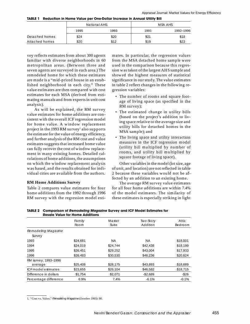
To demonstrate the “real world” valid-ity of this research, the regression resultshave been compared with the collective judg-ment of real estate agents participating in“cost versus value” surveys conducted byRemodeling Magazine (RM). Each year, the RMsurvey asks agents throughout the UnitedStates to estimate the amount that popularremodeling projects would add to the valueof a home in their area if the home were soldwithin a year of project completion. This sur-


455

TABLE 1 Reduction in Home Value per One-Dollar Increase in Annual Utility Bill

National AHS MSA AHS

1995 1993 1991 1992–1996

Detached homes $24 $20 $21 $18Attached homes $20 $12 $19 $23

vey reflects estimates from about 300 agentsfamiliar with diverse neighborhoods in 60metropolitan areas. (Between three andseven agents are surveyed in each area.) Theremodeled home for which these estimatesare made is a “mid-priced house in an estab-lished neighborhood in each city.” Thesevalue estimates are then compared with costestimates for each MSA (derived from esti-mating manuals and from experts in unit costanalysis).

As will be explained, the RM surveyvalue estimates for home additions are con-sistent with the overall ICF regression modelfor home value. A window replacementproject in the 1993 RM survey1 also supportsthe estimate for the value of energy efficiency,and further analysis of the RM cost and valueestimates suggests that increased home valuecan fully recover the cost of window replace-ment in many existing homes. Detailed cal-culations of home additions, the assumptionson which the window replacement analysiswas based, and the results obtained for indi-vidual cities are available from the authors.

RM Home Additions SurveyTable 2 compares value estimates for fourhome additions from the 1992 through 1996RM survey with the regression model esti-

mates. In particular, the regression valuesfrom the MSA detached home sample wereused in the comparison because this regres-sion was taken of the largest AHS sample andshowed the highest measures of statisticalsignificance in our study. The value estimatesin table 2 reflect changes in the following re-gression variables:

• The number of rooms and square foot-age of living space (as specified in theRM survey);

• The estimated change in utility bills(based on the project’s addition to liv-ing space relative to the average size andutility bills for detached homes in theMSA sample); and

• The living space and utility interactionmeasures in the ICF regression model(utility bill multiplied by number ofrooms, and utility bill multiplied bysquare footage of living space).

Other variables in the model (lot size, ageof unit, and location) are not reflected in table2 because these variables would not be af-fected by an addition to an existing home.

The average RM survey value estimatesfor all four home additions are within 7.4%of the model estimates. The similarity ofthese estimates is especially striking in light

1. “Cost vs. Value,” Remodeling Magazine (October 1993): 90.

Nevin/Bender/Gazan: Construction and the Appraiser

TABLE 2 Comparison of Remodeling Magazine Survey and ICF Model Estimates forResale Value for Home Additions

Family Master Two-Story AtticRoom Suite Addition Bedroom

Remodeling MagazineSurvey

1993 $24,681 NA NA $18,0011994 $24,019 $24,744 $42,438 $18,1991995 $26,451 $29,252 $43,004 $17,9331996 $26,483 $30,530 $46,236 $20,624RM survey, 1993–1996

average $25,408 $28,175 $43,893 $18,689ICF model estimates $23,655 $26,104 $46,582 $18,715Difference in dollars $1,754 $2,071 -$2,689 -$26Percentage difference 6.9% 7.4% -6.1% -0.1%



of the detail provided in the RM survey ques-tions that could not be reflected in the modelestimates. For example, the master suite de-scribed in the 1994 RM survey is “a 24-foot-by-16-foot master bedroom with walk-incloset, dressing area, master bath, whirlpooltub, separate ceramic tile shower and double-bowl vanity.” The model estimate, by con-trast, reflects only the value of adding any382-square-foot room, and the associatedchange in the home’s annual utility bill. Inspite of the generic nature of the model, thereis actually more variation between the an-nual RM survey estimates than there is be-tween the average RM estimates and themodel estimates.

Window Replacement ComparisonIn 1993 Remodeling Magazine did a survey onthe value of window replacement. The RMwindow replacement project would “replace16 existing 3-foot-by-5-foot windows withenergy-efficient vinyl or vinyl-clad alumi-num double-pane windows.” To determinewhether the RM value estimates for thisproject were largely attributable to the en-ergy savings, we performed an analysis thatincluded the following four steps:

1. Specifying model home energy use char-acteristics consistent with the RM sur-vey question for windows

2. Estimating pre-project utility bills usingthe (Department of Energy’s) DOE2 en-ergy analysis program, and validatingthese estimates against actual bills re-ported in the AHS

3. Estimating post-project utility bills andcalculating utility bill savings for differ-ent types of windows

4. Multiplying annual utility savings timesthe model value for utility bill, and com-paring these window replacement valueestimates with RM survey value esti-mates

These four steps were repeated for ev-ery MSA included in both the RM survey andin the AHS MSA sample. In all, 25 MSAswere included, providing a range of geo-graphic and climate scenarios to test the re-gression estimate for the value of energy ef-ficiency. The MSAs were:

• East: Boston, Providence, Pittsburgh, Bal-timore/Washington, D.C., and Hartford

• South: New Orleans, Dallas, Birming-ham, Charlotte, and Atlanta

• Midwest: Columbus, Kansas City, Mil-waukee, St. Louis, Minneapolis, Detroit,Cleveland, and Indianapolis

• West: San Diego, Denver, Salt Lake City,Phoenix, Seattle, San Francisco, and Port-land

Model home specifications for thisanalysis were designed to approximate his-torical construction practices and reflect thedescription of remodeled homes in the RMsurvey. The model home in each city wasassumed to have floor space equal to theAHS median square footage for single-fam-ily detached homes in that MSA, reflectingthe RM survey description of a “mid-pricedhouse.” The analysis also specifies 240 squarefeet of windows, based on the RM descrip-tion of replacing sixteen 3-foot-by 5-foot win-dows. The model home is assumed to haverelatively little wall insulation because theRM survey describes a home in an “estab-lished neighborhood” and agents respond-ing to the survey are likely to think aboutolder homes when asked about window re-placement. Older homes and especially thosebuilt before the oil shocks of 1973 and 1979are likely to have less insulation than newerhomes. Ceilings are assumed to have some-what more insulation because ceiling insu-lation has been added to many older homessince the 1973 and 1979 spikes in fuel prices.

To reflect somewhat different regionalconstruction practices, homes in the Southand West were assumed to have a 28% ductloss, whereas homes in the East and Midwestwere assumed to have a 20% duct loss. En-ergy efficiency assumptions for heating andcooling were based on estimates from theHome Energy Rating Systems Council. TheDOE2 energy analysis program was used toestimate model home energy demand withand without air conditioning, and with eachof four heating system types (electric resis-tance, heat pump, natural gas furnace, andoil furnace). Weighted average energy de-mand for each city was calculated based onAHS data showing the percentage of pre-1980 single-family detached homes in eachMSA with air conditioning and each type ofheating system. Data from the 1993 Residen-tial Energy Consumption Survey (RECS), pre-sented in table 3, show that pre-1980 homesaccount for practically all of the homes thatreported replacement of all original win-dows. Therefore, real estate agents respond-ing to the 1993 RM Survey must have madevalue estimates for window replacements


457

based on their experience with pre-1980homes.

Energy consumption associated with hotwater was estimated to reflect typical unitsin the AHS MSA data for single-family de-tached homes built before 1980. Energy con-sumption for other uses of electricity wasbased on estimates from the Home EnergyRatings Systems Council.

Table 4 presents the model home speci-fications that would change as a result of thewindow replacement project. Separate DOE2model estimates for homes before windowreplacement were developed to illustrate thesignificant difference in energy use for homeswith wood-frame windows versus homeswith metal-frame windows. The pre-projectspecifications reflect RECS data indicatingthat most pre-1980 homes in the East andMidwest have storm windows, but mosthomes in the West and South do not. TheRECS data also show that single-pane win-dows are the norm for pre-1980 homes in allregions. The infiltration rate in homes beforewindow replacement was assumed to be oneair change per hour, and the window replace-ment project was expected to reduce the in-filtration rate to 0.7 air changes per hour.

Post-project double-pane windows withclear glass were expected to be the basis forvalue estimates in the RM survey becausehigh-performance low-emissivity (low-e)

TABLE 3 Age Distribution of Homes with All Original Windows Replaced

Year of HomeConstruction Northeast Midwest South West

Pre-1940 38% 45% 22% 15%1940–1949 8% 14% 13% 20%1950–1959 32% 17% 35% 43%1960–1969 15% 21% 11% 13%1970–1979 5% 3% 10% 6%Post-1980 2% 0% 9% 3%

100% 100% 100% 100%Percentage of all homes with

all windows replaced 22% 12% 7% 7%

Source: Residential Energy Consumption Survey, 1993.

windows were not widely used before the1990s. RECS data show that low-e windowsaccount for less than 5% of all replacementwindows installed before 1993. Therefore,this analysis examines whether the energysavings with clear-glass, double-pane win-dows can substantially explain the RM sur-vey value estimates. The additional energysavings with low-e windows are then calcu-lated to show how additional home value canbe realized with the choice of high-perfor-mance windows. Two different high-perfor-mance windows were examined to yield thebest performance in warm or cold climates.

The model home specifications just de-scribed were used to estimate annual energyconsumption for homes before window re-placement in each MSA, and these estimateswere multiplied by 1993 energy prices to es-timate utility bills before window replace-ment. MSA energy prices were approximatedwith available data on 1993 statewide aver-ages for residential prices from the EnergyInformation Administration. Table 5 showsAHS average utility bills and the estimatedutility bills for two pre-project model homesin each region, with wood- and metal-framewindows.

The regional average for DOE2 modelutility bills in homes with wood-frame win-dows are within 14% of the average utilitybills reported in the AHS MSA data. The RECS

TABLE 4 Model Home Specifications for Window Replacement

Region Pre-Project Specification Post-Project Specification

East and Midwest windows Single-pane with storm Clear glass, double-pane(DOE2 glass values) (U-0.57, SC-0.96, SHGC-0.83) (U-0.49, SC-0.89, SHGC-0.76)

South and West windows Single-pane, without storm or High Performance Low-eU-1.09, SC-0.95, SHGC-0.81 (U-0.29, SC-0.33, SHGC-0.29 or

U-0.24, SC-0.5, SHGC-0.44Infiltration rate 1.0 air change per hour 0.7 air change per hour




data in table 6 show that non-metal framesare most common in older homes, and aretherefore more likely to be the basis for theRM survey estimates. The DOE2 model billsshould be somewhat higher than the AHSaverage because the model home bills reflectthe average for pre-1980 homes with single-pane windows. Although RECS data indicatethat about 70% of pre-1980 homes have single-pane glass in most windows, the 30% that re-port double-pane glass in most windowswould tend to reduce the average utility billsin the AHS data. The DOE2 model bills in theSouth are somewhat lower than the actualAHS bills, indicating that the DOE2 modelhome specifications for this analysis mayslightly overstate the energy efficiency of av-erage homes in the South.

Table 7 presents the DOE2 estimatedannual utility bill savings from the windowreplacement project described in the 1993 RMsurvey. Four estimates were calculated for

each region, showing the annual savings as-sociated with replacing wood- or metal-frame, single-pane windows with clear-glass,double-pane windows or high-performancelow-e windows.

The 25 MSA average shows that the en-ergy savings from replacing wood-frame,single-pane windows with clear-glass,double-pane windows is $200 per year, andthe energy savings from replacing metal-frame, single-pane windows is $310 per year.Using high-performance low-e replacementwindows increases annual savings by anadditional $114 per year.

Table 8 compares the RM survey esti-mates for window replacement value withthe ICF model estimates for clear-glass,double-pane replacement windows. The ICFestimates reflect the savings in the annualutility bill resulting from clear-glass, double-pane windows (from table 7) multiplied by$20 (based on the ICF conclusion that home

TABLE 6 Percent of Homes with Non-Metal Frames in Most Windows

Year of Construction Northeast Midwest South West

Pre-1940 84% 87% 78% 65%1940–1949 68% 82% 68% 50%1950–1959 75% 72% 45% 44%1960–1969 71% 62% 36% 15%1970–1979 71% 72% 31% 13%

Source: Residential Energy Consumption Survey.

TABLE 5 DOE2 Estimated Utility Bill for Pre-Project Model Home VersusActual AHS Average Utility Bills

DOE2 AHSEstimated Average Annual Percentage

Annual Utility Bill Utility Bill Difference

Metal frame Wood frame Metal frame Wood frame

East $2,057 $1,922 $1,774 -16% -8%South $1,575 $1,471 $1,598 1% 8%Midwest $1,742 $1,626 $1,428 -22% -14%West $1,429 $1,337 $1,200 -19% -11%25-MSA average $1,684 $1,573 $1,467 -15% -7%

Source: American Housing Survey data and DOE2.

TABLE 7 DOE2 Estimated Annual Utility Bill Savings from Window Replacement

High-PerformancePost-Project Window: Clear-Glass Double-Pane Low-e

Pre-Project Window: Metal frame Wood frame Metal frame Wood frame

East $337 $202 $419 $284South $312 $208 $503 $399Midwest $302 $186 $396 $280West $299 $207 $404 $31225-MSA average $310 $200 $424 $314

Source: Remodeling Magazine.


459

value increases by $20 for every dollar re-duction in annual utility bills).

The 25 MSA average shows that the en-ergy savings from replacing wood-frame,single-pane windows with clear-glass,double-pane windows explains 73% of theRM survey value estimates for this project.The energy savings from replacing metal-frame, single-pane windows with clear-glass,double-pane windows could increase homevalue by 113% of the RM survey value esti-mates. As noted before, the RM survey pri-marily should reflect the experience of realestate agents with the value of replacingwood-frame windows because older homesaccount for most of the homes that have re-placed all original windows, and older homesare more likely to have wood-frame windows.

The results in table 9 indicate that the RMsurvey value estimates for window replace-ment can be substantially explained by themarket value of energy efficiency estimatedby ICF. The 25 MSA average values indicatethat about $4,000 of the RM survey windowreplacement value may be due to energy ef-ficiency, and about $1,500 to the value as-cribed to the ease of use and the appearanceof new windows.

The difference between the model value(for wood frame) and the RM survey value isonly $435 in the South, but this may reflectlimitations of the RM survey data. RECS dataindicate that only 7% of homes in the Southreport that all their original windows havebeen replaced so that real estate agents re-sponding to the RM survey in this region mayhave relatively little experience with the mar-ket value of window replacement. Further,AHS data show that the percentage of pre-1980, single-family detached homes in theSouth with central air conditioning increasedfrom 49% in 1985 to 66% in 1995. Therefore,the response of real estate agents in the Southwho estimate the value of window replace-

ment based on their career experience mayreflect the lesser value of energy-efficienthomes associated with years when fewerhomes had central air conditioning.

The 1993 RM survey concludes that win-dow replacement only recovers about 70%of project costs, on average, but the data intable 8 suggest that RM value estimates mayrepresent only the value of replacing wood-frame windows with clear-glass, double-pane windows. Significantly greater energy-efficiency value could be realized by replac-ing metal-frame windows, and even greaterenergy savings would be realized with high-performance low-e windows. Therefore, theRM survey may accurately reflect the histori-cal cost recovery percentage for window re-placement but may understate the potentialcost recovery with more efficient windows.

Table 9 compares the RM estimates forwindow replacement cost with our energyvalue estimates for high-performance win-dows (based on annual utility savings withhigh-efficiency windows multiplied by $20).The 25-MSA average shows that the valueassociated with energy savings from high-efficiency windows could recover more than85% of the cost of replacing wood-frame,single-pane windows and 115% of the costof replacing metal-frame windows.

Although older homes with wood-framewindows account for most of the homes thathave already replaced all original windows,RECS data indicate that about half of all ex-isting homes have metal-frame windows.Table 9 suggests that replacing metal-framewindows with high-performance windowscould result in an energy-efficient home valuethat exceeds the cost of window replacement.

In the case of wood-frame windows, table9 indicates that the average cost of windowreplacement is about $1,100 more than the ICFmodel value for high-performance windows.RM cost estimates in table 9 may also under-


TABLE 8 ICF Estimated Energy Value for Clear-Glass Double-Pane Windows VersusRemodeling Magazine Survey Value Estimates for Window Replacement

ICF Model Values RM Survey ICF Modelfor Clear-Glass Value Percentage ofDouble-Pane Estimates RM Survey Value


East $6,744 $4,048 $6,372 106% 64%South $6,248 $4,160 $4,595 136% 91%Midwest $6,035 $3,718 $5,757 105% 65%West $5,989 $4,149 $5,118 117% 81%25-MSA average $6,206 $3,993 $5,469 113% 73%




state the higher cost of low-e windows by about$240 (an additional dollar per square foot ofwindow area). On the other hand, the ICFmodel values in table 9 reflect only the valueof energy efficiency, and the analysis of table 8concluded that the appearance value of newwindows makes up about $1,500 of the valueof energy efficiency. The net effect of these fac-tors suggests that the total value of new high-performance low-e windows may also fullyrecover the cost of window replacement inhomes with wood-frame windows.

CONCLUSION

The validity of the overall model for homevalue is substantiated by the comparisonwith value estimates of home additions pro-

vided by real estate agents participating inthe “cost versus value” survey by Remodel-ing Magazine. Detailed analysis of the RMsurvey on a window replacement project alsoindicates that the value estimates from win-dow replacement can be substantially ex-plained by the market value of energy effi-ciency, as estimated in the regression analy-sis. This analysis also indicates that the RMsurvey appears to reflect the historical recov-ery of window replacement cost, but mayunderstate the potential cost recovery withmore efficient windows. In fact, this analy-sis shows that the value associated with high-performance low-e windows could fully re-cover the cost of replacing wood-frame,single-pane windows and may well exceedthe cost of replacing metal-frame windows.

TABLE 9 ICF Estimated Energy Value of High-Performance Low-e Windows VersusRM Survey Cost Estimates for Window Replacement

ICF Model Values RM Survey ICF Modelfor Clear-Glass Cost Percentage ofDouble-Pane Estimates RM Survey Cost


East $8,376 $5,680 $7,764 108% 73%South $10,064 $7,976 $6,455 156% 124%Midwest $7,920 $5,603 $7,571 105% 74%West $8,083 $6,243 $7,642 106% 82%25-MSA average $8,486 $6,272 $7,406 115% 85%



Background

The market for photovoltaic (PV) energy

systems is expanding rapidly in the U.S.

Almost 100,000 PV systems have been

installed in California alone, more than

90% of which are residential. Some of

those “PV homes” have sold, yet little

research exists estimating if those homes

sold for significantly more than similar

non-PV homes. A clearer understanding

of these effects might influence the deci-

sions of homeowners considering install-

ing PV on their home or selling their

home with PV already installed, of home

buyers considering purchasing a home

with PV already installed, and of new

home builders considering installing PV

on their production homes.

To determine whether PV homes sell for

significantly more than comparable non-

PV homes, Berkeley Lab analyzed a

dataset of approximately 72,000 Califor-

nia homes, almost 2,000 of which had

PV systems installed at the time of sale.

The study also investigated whether pre-

miums for PV installed on new homes

were different than those for PV in-

stalled as a retrofit on existing homes,

and whether the age or the size of the PV

system impacted premiums.

A large number of hedonic pricing and

difference-in-difference models (see

sidebar on next page) were used to en-

sure that the results were robust.

Results

The research finds strong evidence that

homes with PV systems in California

have sold for a premium over compara-

ble homes without PV systems. More

specifically, estimates for average PV

premiums among a large number of dif-

ferent model specifications coalesced

near $17,000 for a relatively new

“average-sized” - based on the sample of

homes studied - PV system of 3,100

watts (DC). This corresponds to an aver-

age home sales price premium of $5.5/

watt (DC), with the range of results

across various models being $3.9 to

$6.4/watt.

These results are similar to the average

increase for PV homes found by Dastrop

et al. (2010), which used similar meth-

ods but focused on homes in the San

Diego area. The average sales price pre-

miums also appear to be comparable to

the investment that homeowners have

made to install PV systems in California

(after applicable state and federal incen-

tives), which from 2001-2009 averaged

approximately $5/watt (DC) (Barbose et

al., 2010), and homeowners with PV

also benefit from electricity cost savings

after PV system installation and prior to

home sale.

When the dataset is split between new

and existing homes, PV system premi-

ums are found to be markedly affected

(see figure on back), with new homes

with PV demonstrating average premi-

ums of $2.3 to 2.6/watt, while the aver-

age premium for existing homes with

PV being more than $6/watt. The report

offers a number of possible explanations

for why this disparity might exist, in-

cluding differences in the underlying net

installation costs for PV systems be-

tween new and existing homes. Addi-

tionally, new home builders may gain

value from PV as a market differentiator,

and have therefore often tended to sell

ERNEST

ORLANDO

LAWRENCE

BERKELEY

NATIONAL

LABORATORY

REPORT LBNL-4476E

An Analysis of the Effects of

Residential

Photovoltaic Energy

Systems on Home Sales Prices

in California

Ben Hoen, Ryan Wiser ,

Peter Cappers, and Mark Thayer

Environmental Energy

Technologies Division

April 2011

The report can be downloaded from: http://eetd.lbl.gov/ea/emp/reports/lbnl-

4476e.pdf

This work was supported by the Office of Energy

Efficiency and Renewable Energy (Solar Energy

Technologies Program) of the U.S. Department of

Energy under Contract No. DE-AC02-05CH11231, by

the National Renewable Energy Laboratory under

Contract No. DEK-8883050, and by the Clean Energy

States Alliance.

Research Report Summary

An Analysis of the Effects of Residential

Photovoltaic Energy Systems on Home Sales Prices

in California

Berkeley Lab Summary

http://eetd.lbl.gov/ea/emp/reports/lbnl-4476e.pdf

http://eetd.lbl.gov/ea/emp/reports/lbnl-4476e.pdf

PV as a standard (as opposed to an op-

tional) product on their homes and perhaps

been willing to accept a lower premium in

return for faster sales velocity and de-

creased carrying costs.

The research also finds that, as PV sys-

tems age, the premium enjoyed at the time

of home sale decreases, indicating that

buyers and sellers of PV homes may be

accounting for the decreased efficiency

and remaining expected life of older PV

systems.

When the results are expressed as a ratio

of the sales price premium to estimated

annual electricity cost savings associated

with PV (see figure below) they are con-

sistent with

those of the

m o r e -

e x t e n s i v e

existing lit-

erature on the

impact of

energy effi-

ciency on

home sales

prices; the

present re-

search finds

an averages

range from

7:1 to 31:1, with models coalescing near

20:1.

Applicability

Although this research finds strong evi-

dence that homes with PV systems in Cali-

fornia have sold, on average, for a signifi-

cant premium over comparable homes

without PV systems, the authors recom-

mend that extrapolation of these results to

different locations or market conditions be

done with care.

Further Research Warranted

The report outlines a number of additional

questions that warrant further research,

such as investigating more-recent home

sales (the report’s dataset spanned 1999

thru 2009) from a broader geographic area

(the dataset included only California

homes), and further investigating the dif-

ference in premium between new and ex-

isting PV homes.

What Is a Hedonic Pricing Model?

Hedonic pricing models are fre-

quently used by real estate profes-

sionals and academics to assess the

impacts of individual house and com-

munity characteristics on property

values by investigating the sales

prices of homes. A house can be

thought of as a bundle of characteris-

tics (e.g., number of square feet).

When a price is agreed upon between

a buyer and a seller there is an im-

plicit understanding that those charac-

teristics have value. When data from

a large group of residential transac-

tions are available, the average mar-

ginal contribution to the sales price of

each characteristic can be estimated

with a regression model. The contri-

bution to the selling price of having a

PV system can be thus be estimated,

if other important housing market

influences are adequately controlled

for.

What Is a Difference-in-Difference

Model?

A variant of the hedonic model, a

difference-in-difference model com-

pares inflation adjusted selling prices

of homes that have sold twice, both

before a condition exists (e.g., having

a PV system installed) and after.

What Are Robustness Models?

Because models are built on assump-

tions, practitioners often test those

assumptions by trying multiple model

forms. In this research, “base” mod-

els, which used the full dataset and

controlled for “neighborhood” effects

at the census block group level, were

compared with “robustness” models.

Examples include models that con-

trolled for “neighborhood” at the

subdivision level (a potentially better

proxy than the block group), models

that “matched” PV and non-PV

homes to be statistically identical in

many respects (similar to what an

appraiser might do when valuing a

home), and models that only evalu-

ated PV homes.

The general consistency in results

across all of the models demonstrates

the robustness of the study’s findings.

References

Dastrop, S., Zivin, J. G., Costa, D. L. and Kahn, M. E.

(2010) Understanding the Solar Home Price Premium:

Electricity Generation and “Green” Social Status. UC

Center for Energy & Env. Econ., Berkeley, CA. Dec 9, 10.

WP-001.

Barbose, G., Darghouth, N. and Wiser, R. (2010) Tracking

the Sun III: The Installed Cost of Photovoltaics in the U.S.

1998-2009. LBNL, Berkeley, CA. Dec, 10. LBNL-4121E.

$5.8 $5.6 $4.8

$2.3 $2.6 $2.6

$7.7 $6.5 $6.4

$0

$1

$2

$3

$4

$5

$6

$7

$8

$9

$10

Base

Hedonic Models

Subdivision Robustness

Hedonic Models

Matched Robustness

Hedonic Models

Esti

mat

ed S

ale

Pri

ce P

rem

ium

Fo

r P

V H

om

es

(in

$/W

att

DC

)

All Homes

New Homes

Existing Homes

Berkeley Lab Summary

LBNL-4476E

An Analysis of the Effects of Residential Photovoltaic Energy Systems on Home Sales Prices in California Ben Hoen, Ryan Wiser, Peter Cappers and Mark Thayer Environmental Energy Technologies Division April 2011 Download from http://eetd.lbl.gov/ea/emp/reports/lbnl-4476e.pdf This work was supported by the Office of Energy Efficiency and Renewable Energy (Solar Energy Technologies Program) of the U.S. Department of Energy under Contract No. DE-AC02-05CH11231, by the National Renewable Energy Laboratory under Contract No. DEK-8883050, and by the Clean Energy States Alliance.

ERNEST ORLANDO LAWRENCE BERKELEY NATIONAL LABORATORY

Berkeley Lab Report

Disclaimer

This document was prepared as an account of work sponsored by the United States Government. While this document is believed to contain correct information, neither the United States Government nor any agency thereof, nor The Regents of the University of California, nor any of their employees, makes any warranty, express or implied, or assumes any legal responsibility for the accuracy, completeness, or usefulness of any information, apparatus, product, or process disclosed, or represents that its use would not infringe privately owned rights. Reference herein to any specific commercial product, process, or service by its trade name, trademark, manufacturer, or otherwise, does not necessarily constitute or imply its endorsement, recommendation, or favoring by the United States Government or any agency thereof, or The Regents of the University of California. The views and opinions of authors expressed herein do not necessarily state or reflect those of the United States Government or any agency thereof, or The Regents of the University of California. Ernest Orlando Lawrence Berkeley National Laboratory is an equal opportunity employer.

Berkeley Lab Report

i

LBNL-4476E

An Analysis of the Effects of Residential Photovoltaic Energy Systems on Home Sales Prices in California

Prepared for the

Office of Energy Efficiency and Renewable Energy Solar Energy Technologies Program

U.S. Department of Energy

and the

National Renewable Energy Laboratory

and the

Clean Energy States Alliance

Principal Authors:

Ben Hoen, Ryan Wiser and Peter Cappers Ernest Orlando Lawrence Berkeley National Laboratory

1 Cyclotron Road, MS 90R4000 Berkeley, CA 94720-8136

Mark Thayer

San Diego State University 5500 Campanile Dr.

San Diego, CA 92182-4485

April 2011

This work was supported by the Office of Energy Efficiency and Renewable Energy (Solar Energy Technologies Program) of the U.S. Department of Energy under Contract No. DE-AC02-05CH11231, by the National Renewable Energy Laboratory under Contract No. DEK-8883050, and by the Clean Energy States Alliance.

Berkeley Lab Report

ii

Acknowledgements

This work was supported by the Office of Energy Efficiency and Renewable Energy (Solar Energy Technologies Program) of the U.S. Department of Energy under Contract No. DE-AC02-05CH11231, by the National Renewable Energy Laboratory under Contract No. DEK-8883050, and by the Clean Energy States Alliance. For funding and supporting this work, we especially thank Jennifer DeCesaro (U.S. DOE), Robert Margolis (NREL), and Mark Sinclair (Clean Energy States Alliance). For providing the data that were central to the analysis contained herein, we thank Cameron Rogers (Fiserv), Joshua Tretter (Core Logic Inc.), Bob Schweitzer (Sammish), Eric Kauffman (CERES), James Lee and Le-Quyen Nguyen (CEC), Steven Franz and Jim Barnett (SMUD), and Sachu Constantine (formerly with the CPUC), all of whom were highly supportive and extremely patient throughout the complicated data aquistion process. Finally, we would like to thank the many external reviewers for providing valuable comments on an earlier draft version of the report. Of course, any remaining errors or omissions are our own.

Berkeley Lab Report

iii

Abstract

An increasing number of homes with existing photovoltaic (PV) energy systems have sold in the

U.S., yet relatively little research exists that estimates the marginal impacts of those PV systems

on home sales prices. A clearer understanding of these effects might influence the decisions of

homeowners considering installing PV on their home or selling their home with PV already

installed, of home buyers considering purchasing a home with PV already installed, and of new

home builders considering installing PV on their production homes. This research analyzes a

large dataset of California homes that sold from 2000 through mid-2009 with PV installed.

Across a large number of hedonic and repeat sales model specifications and robustness tests, the

analysis finds strong evidence that California homes with PV systems have sold for a premium

over comparable homes without PV systems. The effects range, on average, from approximately

$3.9 to $6.4 per installed watt (DC) of PV, with most coalescing near $5.5/watt, which

corresponds to a home sales price premium of approximately $17,000 for a relatively new 3,100

watt PV system (the average size of PV systems in the study). These average sales price

premiums appear to be comparable to the investment that homeowners have made to install PV

systems in California, which from 2001 through 2009 averaged approximately $5/watt (DC), and

homeowners with PV also benefit from electricity cost savings after PV system installation and

prior to home sale. When expressed as a ratio of the sales price premium to estimated annual

electricity cost savings associated with PV, an average ratio of 14:1 to 22:1 can be calculated;

these results are consistent with those of the more-extensive existing literature on the impact of

energy efficiency (and energy cost savings more generally) on home sales prices. The analysis

also finds - as expected - that sales price premiums decline as PV systems age. Additionally,

when the data are split between new and existing homes, a large disparity in premiums is

discovered: the research finds that new homes with PV in California have demonstrated average

premiums of $2.3-2.6/watt, while the average premium for existing homes with PV has been

more than $6/watt. One of several possible reasons for the lower premium for new homes is that

new home builders may also gain value from PV as a market differentiator, and have therefore

often tended to sell PV as a standard (as opposed to an optional) product on their homes and

perhaps been willing to accept a lower premium in return for faster sales velocity. Further

research is warranted in this area, as well as a number of other areas that are highlighted.

Berkeley Lab Report

iv

Table of Contents

1. Introduction ............................................................................................................................. 1

2. Data Overview ........................................................................................................................ 6 2.1. Data Sources ................................................................................................................... 6 2.2. Data Processing ............................................................................................................... 8 2.3. Data Summary .............................................................................................................. 10

3. Methods and Statistical Models ............................................................................................ 17 3.1. Methodological Overview ............................................................................................ 17 3.2. Variables Used in Models ............................................................................................. 18 3.3. Fixed and Continuous Effect Hedonic Models ............................................................. 20 3.4. New and Existing Home Models .................................................................................. 24

3.4.1. Difference-in-Difference Models .......................................................................... 24 3.5. Age of the PV System for Existing Homes Hedonic Models ....................................... 27 3.6. Returns to Scale Hedonic Models ................................................................................. 28 3.7. Model Summary............................................................................................................ 30

4. Estimation Results ................................................................................................................ 31 4.1. Fixed and Continuous Effect Hedonic Model Results .................................................. 32 4.2. New and Existing Home Model Results ....................................................................... 35

4.2.1. Difference-in-Difference Model Results .............................................................. 39 4.3. Age of PV System for Existing Home Hedonic Model Results ................................... 41 4.4. Returns to Scale Hedonic Model Results...................................................................... 42

5. Conclusions ........................................................................................................................... 45

References ..................................................................................................................................... 50

Berkeley Lab Report

v

List of Tables

Table 1: Variable Descriptions ..................................................................................................... 10

Table 2: Summary Statistics of Full Dataset ................................................................................. 12

Table 3: Summary Statistics of Repeat Sale Dataset .................................................................... 13

Table 4: Frequency Summary by California County .................................................................... 14

Table 5: Frequency Summary by Home Type, Utility and Sale Year .......................................... 16

Table 6: Difference-in-Difference Description ............................................................................. 25

Table 7: Summary of Models ....................................................................................................... 30

Table 8: Fixed and Continuous Base Hedonic Model Results with Robustness Tests ................. 35

Table 9: New and Existing Home Base Hedonic Model Results with Robustness Tests............. 38

Table 10: Difference-in-Difference Model Results ...................................................................... 41

Table 11: Age of PV System and Return to Scale Hedonic Model Results ................................. 44

List of Figures

Figure 1: Map of Frequencies of PV Homes by California County ............................................. 15

Figure 2: Fixed and Continuous Effect Base Model Results with Robustness Tests ................... 33

Figure 3: New and Existing Home Base Model Results with Robustness Tests .......................... 36

Figure 4: Existing Home Hedonic and Difference-in-Difference Model Results with Robustness

Tests .............................................................................................................................................. 40

Figure 5: Estimated Ratios of Sale Price Premium to Annual Energy Cost Savings ................... 48

Berkeley Lab Report

1

1. Introduction

In calendar year 2010, approximately 880 megawatts (MW)1

of grid-connected solar

photovoltaic (PV) energy systems were installed in the U.S. (of which approximately 30% were

residential), up from 435 MW installed in 2009, yielding a cumulative total of 2,100 MW (SEIA

& GTM, 2011). California has been and continues to be the country’s largest market for PV,

with nearly 1000 MW of cumulative capacity. California is also approaching 100,000 individual

PV systems installed, more than 90% of which are residential. An increasing number of these

homes with PV have sold, yet to date, relatively little research has been conducted to estimate the

existence and level of any premium to sales prices that the PV systems may have generated. One

of the primary incentives for homeowners to install a PV system on their home, or for home

buyers to purchase a home with a PV system already installed, is to reduce their electricity bills.

However, homeowners cannot always predict if they will own their home for enough time to

fully recoup their PV system investment through electricity bill savings. The decision to install a

PV system or purchase a home with a PV system already installed may therefore be predicated,

at least in part, on the assumption that a portion of any incremental investment in PV will be

returned at the time of the home’s subsequent sale through a higher sales price. Some in the

solar industry have recognized this potential premium to home sales prices, and, in the absence

of having solid research on PV premiums, have used related literature on the impact of energy

efficiency investments and energy bill savings on home prices as a proxy for making the claim

that residential PV systems can increase sales prices (e.g., Black, 2010).

The basis for making the claim that an installed PV system may produce higher residential

selling prices is grounded in the theory that a reduction in the carrying cost of a home will

translate, ceteris paribus, into the willingness of a buyer to pay more for that home. Underlying

this notion is effectively a present value calculation of a stream of savings associated with the

1 All references to the size of PV systems in this paper, unless otherwise noted, are reported in terms of direct current (DC) watts under standard test conditions (STC). This convention was used to conform to the most-common reporting conventions used outside of California. In California, PV systems sizes are often referred to using the California Energy Commission Alternating Current (CEC-AC) rating convention, which is approximately a multiple of 0.83 of the DC-STC convention, but depends on a variety of factors including inverter efficiency and realistic operating efficiencies for panels. A discussion of the differences between these two conventions and how conversions can be made between them is offered in Appendix A of Barbose et al., 2010.

Berkeley Lab Report

2

reduced electricity bills of PV homes, which can be capitalized into the value of the home.

Along these lines, a number of studies have shown that residential selling prices are positively

correlated with lower energy bills, most often attributed to energy related home improvements,

such as energy efficiency investments (Johnson and Kaserman, 1983; Longstreth et al., 1984;

Laquatra, 1986; Dinan and Miranowski, 1989; Horowitz and Haeri, 1990; Nevin and Watson,

1998; Nevin et al., 1999). The increased residential sales prices associated with lower energy

bills and energy efficiency measures might be expected to apply to PV as well. Some

homeowners have stated as much in surveys (e.g., CEC, 2002; McCabe and Merry, 2010),

though the empirical evidence supporting such claims is limited in scope. Farhar et al. (2004a;

2008) tracked repeat sales of 15 “high performance” energy efficient homes with PV installed

from one subdivision in San Diego and found evidence of higher appreciation rates, using simple

averages, for these homes over comparable homes (n=12). More recently, Dastrop et al. (2010)

used a hedonic analysis to investigate the selling prices of 279 homes with PV installed in the

San Diego, California metropolitan area, finding clear evidence of PV premiums that averaged

approximately 3% of the total sales price of non-PV homes, which translates into $4.4 per

installed PV watt (DC).

In addition to energy savings, higher selling prices might be correlated with a “cachet value”

based on the “green” attributes that come bundled with energy-related improvements (e.g.,

helping combat global warming, impressing the neighbors, etc.). A number of recent papers

have investigated this correlation. Eichholtz et al. (2009, 2011) analyzed commercial green

properties in the U.S, and Brounen and Kok (2010) and Griffin et al. (2009) analyzed green

labeled homes in the Netherlands and Portland, Oregon, respectively, each finding premiums,

which, in some cases, exceeded the energy savings (Eichholtz et al., 2009, 2011; Brounen and

Kok, 2010). Specifically related to PV, Dastrop et al. (2010) found higher premiums in

communities with a greater share of Toyota Prius owners and college grads, indicating,

potentially, the presence of a cachet value to the systems over and above energy savings. It is

therefore reasonable to believe that buyers of PV homes might price both the energy savings and

the green cachet into their purchase decisions.

Berkeley Lab Report

3

Of course there is both a buyer and

a seller in any transaction, and the sellers of PV homes might

be driven by different motivations than the buyers. Specifically, recouping the net installed cost

of the PV system (i.e., the cost of PV installation after deducting any available state and federal

incentives) might be one driver for sellers. In California, the average net installed cost of

residential PV hovered near $5/watt (DC) from 2001 through 2009 (Barbose et al., 2010).

Adding slightly to the complexity, the average net installed cost of PV systems has varied to

some degree by the type of home, with PV systems installed on new homes in California

enjoying approximately a $1/watt lower average installed cost than PV systems installed on

existing homes in retrofit applications (Barbose et al., 2010). Further, sellers of new homes with

PV (i.e., new home developers) might be reluctant to aggressively increase home sale prices for

installed PV systems because of the burgeoning state of the market for PV homes and concern

that more aggressive pricing might slow home sales, especially if PV is offered as a standard (not

optional) product feature (Farhar and Coburn, 2006). At the same time, the possible positive

impact of PV on product differentiation and sales velocity may make new home developers

willing to sell PV at below the net installed cost of the system. After all, some studies that have

investigated whether homes with PV (often coupled with energy efficient features) sell faster

than comparable homes without PV have found evidence of increased velocity due to product

differentiation (Dakin et al., 2008; SunPower, 2008). Finally, as PV systems age, and sellers (i.e.,

homeowners) recoup a portion of their initial investment in the form of energy bill savings (and,

related, the PV system’s lifespan decreases), the need (and ability) to recoup the full initial

investment at the time of home sale might decrease. On net, it stands to reason that premiums

for PV on new homes might be lower than those for existing homes, and that older PV systems

might garner lower premiums than newer PV systems of the same size.

Though a link between selling prices and some combination of energy cost savings, green cachet,

recouping the net installed cost of PV, seller attributes, and PV system age likely exists, the

existing empirical literature in this area, as discussed earlier, has largely focused on either energy

efficiency in residential and commercial settings, or PV in residential settings but in a limited

geographic area (San Diego), with relatively small sample sizes. Therefore, to date, establishing

a reliable estimate for the PV premiums that may exist across a wide market of homes has not

Berkeley Lab Report

4

been possible. Moreover, establishing premiums for new versus existing homes with PV has not

yet been addressed.

Additionally, research has not investigated whether there are increasing or decreasing returns on

larger PV systems, and/or larger homes with the same sized PV systems, nor has research been

conducted that investigates whether older PV systems garner lower premiums. In the case of

returns to scale on larger PV systems, it is not unreasonable to expect that any increase in value

for PV homes may be non-linear as it relates to PV system size. For example, if larger PV

systems push residents into lower electricity price tiers2

, energy bill savings could be diminished

on the margin as PV system size increases. This, in turn, might translate into smaller percentage

increases in residential selling prices as PV systems increase in size, and therefore a decreasing

return to scale. Larger PV systems might also enjoy some economies of scale in installation

costs, which, in turn, might translate into lower marginal premiums at the time of home sale as

systems increase in size – a decreasing return to scale. Additionally, “cachet value”, to the

degree that it exists, is likely to be somewhat insensitive to system size, and therefore might act

as an additional driver to decreasing returns to scale. Somewhat analogously, PV premiums may

be related to the number of square feet of living area in the home. Potentially, as homes increase

in size, energy use can also be expected to increase, leading homeowners to be subjected to

higher priced electricity rate tiers and therefore greater energy bill savings for similarly sized PV

systems. Finally, as discussed previously, as PV systems age, and both a portion of the initial

investment is recouped and the expected life and operating efficiency of the systems decrease,

home sales price premiums might be expected to decline.

To explore these possible relationships, we investigate the residential selling prices across the

state of California of approximately 2,000 homes with existing PV systems against a comparable

set of approximately 70,000 non-PV homes. The sample is drawn from 31 California counties,

with PV home sales transaction dates of 2000 through mid-2009. We apply a variety of hedonic

pricing (and repeat sales) models and sample sets to test and bound the possible effects of PV on

residential sales prices and to increase the confidence of the findings. Using these tools, we also 2 Many California electric utilities provide service under tiered residential rates that charge progressively higher prices for energy as more of it is used.

Berkeley Lab Report

5

explore whether the effects of PV systems on home prices are impacted by whether the home is

new or existing, by the size of either the PV system or the home itself, and finally by how old the

PV system is when the home sells.3 It should be stated that this research is not

intended to

disentangle the specific effects of energy savings, green cachet, recovery of the cost of

installation, or seller motivations, but rather to establish credible estimates of aggregate PV

residential sales price effects.

The paper begins with a discussion of the data used for the analyses (Section 2). This is

followed by a discussion of the empirical basis for the study (Section 3), where the variety of

models and sample sets are detailed. The paper then turns to a discussion of the results and their

potential implications (Section 4), and finally offers some concluding remarks with

recommendations for future research (Section 5).

3 Due to the limited sample of PV home sales in many individual years, the results presented in this report reflect average impacts over the entire 2000-09 period (after controlling for housing market fluctuations).

Berkeley Lab Report

6

2. Data Overview

To estimate the models described later, a dataset of California homes is used that joins the

following five different sets of data: (1) PV home addresses and system information from three

organizations that have offered financial incentives to PV system owners in the state; (2) real

estate information that is matched to those addresses and that also includes the addresses of and

information on non-PV homes nearby; (3) home price index data that allow inflation adjustments

of sale prices to 2009 dollars; (4) locational data to map the homes with respect to nearby

neighborhood/environmental influences; and (5) elevation data to be used as a proxy for “scenic

vista.” Each of these data sources is described below, as are the data processing steps employed,

and the resulting sample dataset.

2.1. Data Sources

The California Energy Commission (CEC), the California Public Utilities Commission (CPUC),

and the Sacramento Municipal Utility District (SMUD) each provide financial incentives under

different programs to encourage the installation of PV systems in residential applications, and

therefore have addresses for virtually all of those systems, as well as accompanying data on the

PV systems.4

Through these programs, Berkeley Laboratory was provided information on

approximately 42,000 homes where PV was installed, only a fraction of which (approximately

9%) subsequently sold with the PV system in place. The data provided included: address (street,

street number, city, state and zip); incentive application and PV system install and operational

dates; PV system size; and delineations as to whether the home was new or existing at the time

the PV system was installed (where available).

4 The CEC and CPUC have both been collecting data on PV systems installed on homes in the utility service areas of investor owned utilities (e.g., PG&E, SCE, SDG&E) for which they have provided incentives, as have some of California’s publicly owned utilities (e.g., SMUD) that offer similar incentives. The CEC began administering its incentive program in 1998, and provided rebates to systems of various sizes for both residential and commercial customers. The CPUC began its program in 2001, initially focusing on commercial systems over 30 kW in size. In January 2007, however, the CEC began concentrating its efforts on new residential construction through its New Solar Home Partnership program, and the CPUC took over the administration of residential retrofit systems through the California Solar Initiative program. Separately, SMUD has operated a long-standing residential solar rebate program, but of smaller size than the efforts of the CEC and CPUC.

Berkeley Lab Report

7

These addresses were then matched to addresses as maintained by Core Logic (CL)5

• address (e.g., street, street number, city, state and zip+4 code);

, which they

aggregate from both the California county assessment and deed recorder offices. Once matched,

CL provided real estate information on each of the California PV homes, as well as similar

information on approximately 150,000 non-PV homes that were located in the same (census)

block group and/or subdivision as the matched PV homes. The data for both of these sets of

homes included:

• most recent (“second”) sale date and amount; • previous (“first”) sale date and amount (if applicable); • home characteristics (where available) (e.g., acres, square feet of living area, bathrooms,

and year built); • assessed value; • parcel land use (e.g., commercial, residential); • structure type (e.g., single family residence, condominium, duplex); • housing subdivision name (if applicable)6

• census tract and census block group. ; and

These data, along with the PV incentive provider data, allowed us to determine if a home sold

after a PV system was installed ("second" sale). 3,657 such homes were identified in total, and

these homes, therefore, represent the possible sample of homes on which our analysis focused.

A subset of these data for which "first" sale information was available and for which a PV

system had not yet been installed as of this “first” sale, were culled out. These “repeat sales”

were also used in the analysis, as will be discussed in Section 3.

In addition to the PV and real estate data, Berkeley Laboratory obtained from Fiserv a zip-code-

level weighted repeat sales index of housing prices in California from 1970 through mid-2009,

by quarter. These indices, where data were available, were differentiated between low, middle,

5 More information about this product can be obtained from http://www.corelogic.com/. Note that Core Logic, Inc. was formerly known as First American Core Logic. 6 In some cases the same subdivisions were referred to using slightly different names (e.g., “Maple Tree Estates” & “Maple Trees Estates”). Therefore, an iterative process of matching based on the names, the zip code, and the census tract were used to create “common” subdivision names, which were then used in the models, as discussed later.

Berkeley Lab Report

http://www.corelogic.com/�

8

and high home price tiers, to accommodate the different appreciation/depreciation rates of

market segments. Using these indices, all sale prices were adjusted to Q1, 2009 prices.7

From Sammamish Data, Berkeley Laboratory purchased x/y coordinates for each zip+4 code,

which allowed the mapping of addresses to street level accuracy.8 Additionally, Berkeley

Laboratory obtained from the California Natural Resources Agency (via the California

Environmental Resources Evaluation System, CERES) a 30 meter level Digital Elevation Map

(DEM) for the state of California.9

2.2. Data Processing

Combining these latter two sets of data, a street level

elevation could be obtained for each home in the dataset, which allowed the construction of a

variable defined as the elevation of a home relative to its (census) block group. This relative

elevation served as a proxy for “scenic vista”, a variable used in the analysis.

Data cleaning and preparation for final analysis was a multifaceted process involving selecting

transactions where all of the required data fields were fully populated, determining if sales of PV

homes occurred after the PV system was installed, matching the homes to the appropriate index,

ensuring the populated fields were appropriately coded, and finally, eliminating obviously

suspicious observations (e.g., not arms length transactions, outliers, etc.). Initially provided were

a total of 150,000 detached single family residential sale records without PV and a total of 3,657

with PV. These totals, however, were substantially reduced (by approximately 65,000 records,

1,400 of which were PV sales) because of missing/erroneous core characteristic data (e.g., sale

date, sale price, year built, square feet).10

7 The inflation adjustment instrument used for this analysis is the Fiserv Case-Shiller Index. This index is a weighted repeat sales index, accumulated quarterly at, optimally, the zip code level over three home price tiers (e.g., low, middle and high prices). More information can be found at:

Additionally, the final dataset was reduced (by

approximately 14,000 records, 300 of which were PV sales) because some sales occurred outside

the range of the index that was provided (January 1970 to June 2009). Moreover, to focus our

analysis on more-typical California homes and minimize the impact of outliers or potential data-

http://www.caseshiller.fiserv.com/indexes.aspx 8 More information about this product can be obtained from http://www.sammdata.com/ 9 More information about this product can be obtained from http://www.ceres.ca.gov/ 10 Examples of “erroneous” data might include a year built or sale date that is in the future (e.g., “2109” or “Jan 1, 2015”, respectively), or large groups of homes that were listed at the same price in the same year in the same block group that were thought to be “bulk” sales and therefore not valid for our purposes.

Berkeley Lab Report

http://www.caseshiller.fiserv.com/indexes.aspx�

http://www.sammdata.com/�

http://www.ceres.ca.gov/�

9

entry errors on our results, observations not

Table 1

meeting the following criteria were screened out (see

for variable descriptions):

• the inflation adjusted most recent (second) sale price (asp2) is between $85,000 and $2,500,000;11

• the number of square feet (sqft) is greater than 750;

• asp2 divided by sqft is between $40 and $1,000; • the number of acres is less than 25 and greater than sqft divided by 43,560 (where one

acre equals 43,560 sqft);12

• the year the home was built (yrbuilt) is greater than 1900;

• the age of the home (in years) at the time of the most recent sale (ages2) is greater than or equal to negative one;

• the number of bathrooms (baths) is greater than zero and less than ten; • the size of the PV system (size) is greater than 0.5 and less than 10 kilowatts (kW); • each block group contains at least one PV home sale and one non-PV home sale; and • the total assessed value (avtotal), as reported by the county via Core Logic, is less than or

equal to the predicted assessed value (pav), where pav = sp2*1.02^(2010-year of sale).13

In addition, the repeat sales used in the analysis had to meet the following criteria:

• the difference in sale dates (sddif) between the most recent (second) sale date (sd2) and the previous (first) sale date (sd1) is less than 20 years;

• PV is not installed on the home as of sd1; and • the adjusted annual appreciation rate (adjaar) is between -0.14 and 0.3 (where adjaar =

ln(asp2/asp1)/(sddif/365), which corresponds to the 5th and 95th percentile for the distribution of adjaar.14

11 An alternative screen was tested that limited the data to homes under $1 million (leaving 90% of the data) and $600,000 (leaving 75%), with no significant change to the results. 12 An alternative screen that incorporated the number of stories for the home along with the number of square feet in calculating the “footprint”, and therefore allowed smaller parcels to be used, was also explored, with no significant change in results. 13 This screen was intended to help ensure that homes that had significant improvements since the most recent sale, which would be reflected in a higher assessed value than would otherwise be the maximum allowable under California property tax law, were removed from the dataset. The screen was not applied to homes that sold in 2009, however, because, in those cases, assessed values often had not been updated to reflect the most recent sale. 14 This final screen was intended to remove homes that had unusually large appreciation or deprecations between sales, after adjusting for inflation, which could indicate that the underlying home characteristics between the two sales changed (e.g., an addition was added, the condition of the home dramatically worsened, etc.), or the data were erroneous.

Berkeley Lab Report

10

Table 1: Variable Descriptions

2.3. Data Summary

The final full dataset includes a total of 72,319 recent sales, 1,894 of which are PV homes and

70,425 of which are non-PV (see Table 2). The homes with PV systems are distributed evenly

between new (51%) and existing (49%) home types, while the non-PV homes are weighted

toward existing homes (62%) over new (38%) (see Table 5). The final repeat sales dataset of

homes selling twice total 28,313 homes, of which 394 are PV and 27,919 are non-PV (see Table

3).

As indicated in Table 2, the average non-PV home in the full sample (not the repeat sales

sample) sold for $584,740 (unadjusted) in late 2005, which corresponds to $480,862 (adjusted)

Variable Descriptionacre size of the parcel (in acres)acregt1 number of acres more than oneacrelt1 number of acres less than oneadjaar adjusted annual appreciation rateages2 age of home as of sd2ages2sqr ages2 squaredasp1 inflation adjusted sp1 (in 2009 dollars)asp2 inflation adjusted sp2 (in 2009 dollars)avtotal total assessed value of the homebath number of bathroomsbgre_100 relative elevation to other homes in block group (in 100s of feet)elev elevation of home (in feet)lasp1 natural log of asp1lasp2 natural log of asp2pav predicted assessed valuepvage age of the PV system at the time of salesd1 first sale datesd2 second sale datesddif number of days separating sd1 and sd2size size (in STC DC kW) of the PV systemsp1 first sale price (not adjusted for inflation)sp2 second sale price (not adjusted for inflation)sqft size of living areasqft_1000 size of living area (in 1000s of square feet)yrbuilt year the home was built

Berkeley Lab Report

11

in 2009 dollars.15 This “average” home is built in 1986, is 19 years old at the time of sale, has

2,200 square feet of living space, has 2.6 bathrooms, is situated on a parcel of 0.3 acres, and is

located at the mean elevation of the other homes in the block group. On the other hand, the

average PV home in the full sample sold for $660,222 in early 2007, which corresponds to

$537,442 in 2009 dollars. Therefore, this “average” PV home, as compared to the “average”

non-PV home, is higher in value. This difference might be explained, in part, by the fact that the

average PV home is slightly younger at the time of sale (by two years), slightly bigger (by 200

square feet), has more bathrooms (by 0.3), is located on a parcel that is slightly larger (by 0.06

acres), and, of course, has a PV system (which is, on average, 3,100 watts and 1.5 years old).16

The repeat sale dataset, as summarized in Table 3, shows similar modest disparities between PV

and non-PV homes, with the “average” PV homes selling for more (in 2009 $) in both the first

and second sales. Potentially more telling, though, non-PV homes show a slight depreciation (of

-1.4%) between sales after adjusting for inflation, while PV homes show a modest appreciation

(of 3.2%). Average PV homes in the sample are found to be slightly bigger (by 100 square feet),

occupy a slightly larger parcel (by 0.2 acres), older (by 10 years), and, of course, have a PV

system (which is, on average, 4,030 watts and 2.5 years old).

Focusing on the full dataset geographically (see Table 4 and Figure 1), we find that it spans 31

counties with the total numbers of PV and non-PV sales ranging from as few as nine (Humboldt)

to as many as 11,991 (Placer). The dataset spans 835 separate (census) block groups (not shown

in the table), though only 162 (18.7%) of these block groups contain subdivisions with at least

one PV sale. Within the block groups that contain subdivisions with PV sales there are 497

subdivision-specific delineations. As shown in Table 5, the data on home sales are fairly evenly

split between new and existing home types, are located largely within four utility service areas,

15 The adjusted values, which are based on a housing price index, demonstrate the large-scale price collapse in the California housing market post 2005; that is, there has been significant housing price depreciation. 16 Age of PV system at the time of sale is determined by comparing the sale date and ideally an “installation date”, which corresponds to the date the system was operational, but, in some cases, the only date obtained was the “incentive application date”, which might precede the installation date by more than one year. For this reason the age of the system reported for this research is lower than the actual age.

Berkeley Lab Report

12

with the largest concentration in PG&E's territory, and occurred over eleven years, with the

largest concentration of PV sales occurring in 2007 and 2008.

In summary, the full dataset shows higher sales prices for the average PV home than the average

non-PV home, while the repeat sales dataset shows positive appreciation between sales for PV

homes, but not for non-PV homes. Though these observations seem to indicate that a PV sales

price premium exists, these simple comparisons do not take into account the other underlying

differences between PV and non-PV homes (e.g., square feet), their neighborhoods, and the

market conditions surrounding the sales. The hedonic and difference-in-difference statistical

models discussed in the following section are designed to do just that.

Table 2: Summary Statistics of Full Dataset

Variable n Mean Std. Dev. Min Maxacre 70425 0.3 0.8 0.0 24.8acregt1 70425 0.1 0.7 0.0 23.8acrelt1 70425 0.2 0.2 0.0 1.0ages2 70425 19 23.3 -1 108ages2sqr 70425 943 1681 0 11881asp2 70425 480,862$ 348,530$ 85,007$ 2,498,106$ avtotal 70425 497,513$ 359,567$ 10,601$ 3,876,000$ bath 70425 2.6 0.9 1 9bgre_100 70425 0.0 1.2 -18.0 19.0elev 70425 424 598 0 5961lasp2 70425 12.9 0.6 11.4 14.7pvage 70425 0 0 0 0sd2 70425 9/30/2005 793 days 1/7/1999 6/30/2009size 70425 0 0 0 0sp2 70425 584,740$ 369,116$ 69,000$ 4,600,000$ sqft_1000 70425 2.2 0.9 0.8 9.3yrbuilt 70425 1986 23 1901 2009

Variable n Mean Std. Dev. Min Maxacre 1894 0.4 1.0 0.0 21.6acregt1 1894 0.1 0.9 0.0 20.6acrelt1 1894 0.2 0.2 0.0 1.0ages2 1894 17.3 24.5 -1 104ages2sqr 1894 937 1849 0 11025asp2 1894 537,442$ 387,023$ 85,973$ 2,419,214$ avtotal 1894 552,052$ 414,574$ 23,460$ 3,433,320$ bath 1894 2.9 1 1 7bgre_100 1894 0.2 1.3 -10.0 17.9elev 1894 414 584 0 5183lasp2 1894 13.0 0.6 11.4 14.7pvage 1894 1.5 2.0 -1.0 9.0sd2 1894 3/28/2007 622 days 8/1/2000 6/29/2009size 1894 3.1 1.6 0.6 10.0sp2 1894 660,222$ 435,217$ 100,000$ 3,300,000$ sqft_1000 1894 2.4 0.9 0.8 11.0yrbuilt 1894 1989 25 1904 2009

Non-PV Homes

PV Homes

Berkeley Lab Report

13

Table 3: Summary Statistics of Repeat Sale Dataset

Variable n Mean Std. Dev. Min Maxacre 27919 0.3 0.7 0.0 23.2acregt1 27919 0.1 0.6 0.0 22.2acrelt1 27919 0.2 0.2 0.0 1.0ages2 27919 23.6 22.7 0 108ages2sqr 27919 1122.0 1775.0 1.0 11881.0asp1 27919 488,127$ 355,212$ 85,398$ 2,495,044$ asp2 27919 481,183$ 347,762$ 85,007$ 2,472,668$ avtotal 27919 498,978$ 360,673$ 35,804$ 3,788,511$ bath 27919 2.5 0.8 1 9bgre_100 27919 0.0 1.3 -17.7 19.0elev 27919 426 588 0 5961lasp1 27919 12.9 0.6 11.4 14.7lasp2 27919 12.9 0.6 11.4 14.7pvage 27919 0 0 0 0sd1 27919 5/5/2001 1780 days 11/1/1984 12/11/2008sd2 27919 5/14/2006 786 days 3/11/1999 6/30/2009sddif 27919 1835 1509 181 7288size 27919 0 0 0 0sp1 27919 444,431$ 287,901$ 26,500$ 2,649,000$ sp2 27919 577,843$ 371,157$ 69,000$ 3,500,000$ sqft_1000 27919 2.1 0.8 0.8 7.7yrbuilt 27919 1982 23 1901 2008

Variable n Mean Std. Dev. Min Maxacre 394 0.5 1.4 0.0 21.6acregt1 394 0.2 1.3 0.0 20.6acrelt1 394 0.2 0.2 0.0 1.0ages2 394 34.6 25.6 1 104ages2sqr 394 1918.0 2336.0 4.0 11025.0asp1 394 645,873$ 417,639$ 110,106$ 2,339,804$ asp2 394 666,416$ 438,544$ 91,446$ 2,416,498$ avtotal 394 682,459$ 478,768$ 51,737$ 3,433,320$ bath 394 2.6 0.9 1 7bgre_100 394 0.1 1.6 -5.5 17.9elev 394 479 581 3 3687lasp1 394 13.2 0.6 11.6 14.7lasp2 394 13.2 0.6 11.4 14.7pvage 394 2.5 1.6 -1.0 9.0sd1 394 11/22/1999 1792 days 11/30/1984 1/7/2008sd2 394 1/9/2007 672 days 8/1/2000 6/29/2009sddif 394 2605 1686 387 7280size 394 4.03 1.94 0.89 10sp1 394 492,368$ 351,817$ 81,500$ 2,500,000$ sp2 394 800,359$ 489,032$ 121,000$ 3,300,000$ sqft_1000 394 2.2 0.8 0.8 5.3yrbuilt 394 1972 26 1904 2008

Non-PV Homes

PV Homes

Berkeley Lab Report

14

Table 4: Frequency Summary by California County

CA County Non-PV PV TotalAlameda 4,826 153 4,979Butte 457 12 469Contra Costa 5,882 138 6,020El Dorado 938 85 1,023Humboldt 7 2 9Kern 2,498 53 2,551Kings 134 5 139Los Angeles 3,368 82 3,450Marin 1,911 61 1,972Merced 48 2 50Monterey 10 2 12Napa 36 1 37Orange 1,581 44 1,625Placer 11,832 159 11,991Riverside 4,262 87 4,349Sacramento 10,928 483 11,411San Bernardino 2,138 50 2,188San Diego 1,083 30 1,113San Francisco 407 16 423San Joaquin 1,807 20 1,827San Luis Obispo 232 1 233San Mateo 2,647 92 2,739Santa Barbara 224 7 231Santa Clara 6,127 157 6,284Santa Cruz 90 1 91Solano 2,413 39 2,452Sonoma 1,246 32 1,278Tulare 774 14 788Ventura 1,643 42 1,685Yolo 16 1 17Yuba 860 23 883

Total 70,425 1,894 72,319

Berkeley Lab Report

15

Figure 1: Map of Frequencies of PV Homes by California County

Berkeley Lab Report

16

Table 5: Frequency Summary by Home Type, Utility and Sale Year

Home Type * Non-PV PV Total New Home 26,938 935 27,873Existing Home 43,487 897 44,384

Utility ** Non-PV PV Total Pacific Gas & Electric (PG&E)

36,137 1,019 37,156

Southern California Edison (SCE)

14,502 337 14,839

San Diego Gas & Electric (SDG&E)

8,191 35 8,226

Sacramento Municipal Utility District (SMUD)

11,393 498 11,891

Other 202 5 207

Sale Year Non-PV PV Total 1999 110 0 1102000 379 1 3802001 1,335 10 1,3452002 6,278 37 6,3152003 8,783 63 8,8462004 10,888 153 11,0412005 10,678 168 10,8462006 9,072 173 9,2452007 8,794 472 9,2662008 9,490 642 10,1322009 4,618 175 4,793

* A portion of the PV homes could not be classified as either new or existing and therefore are not included in these totals** Non-PV utility frequencies were estimated by mapping block groups to utility service areas, and then attributing the utility to all homes that were located in the block group

Berkeley Lab Report

17

3. Methods and Statistical Models

3.1. Methodological Overview

The data, as outlined above, not only show increased sales values and appreciation for PV homes

(in 2009 $) over non-PV homes, but also important differences between PV and non-PV homes

as regards other home, site, neighborhood and market characteristics that could, potentially, be

driving these differences in value and appreciation. A total of 21 empirical model specifications,

with a high reliance on the hedonic pricing model, are used in this paper to disentangle these

potentially competing influences in order to determine whether and to what degree PV homes

sell for a premium.

The basic theory behind the hedonic pricing model starts with the concept that a house can be

thought of as a bundle of characteristics. When a price is agreed upon between a buyer and

seller there is an implicit understanding that those characteristics have value. When data from a

number of sales transactions are available, the average individual marginal contribution to the

sales price of each characteristic can be estimated with a hedonic regression model (Rosen, 1974;

Freeman, 1979). This relationship takes the basic form:

Sales price = f (home and site, neighborhood, and market characteristics)

“Home and site characteristics” might include, but are not limited to, the number of square feet

of living area, the size of the parcel of land, and the presence of a PV system. “Neighborhood”

characteristics might include such variables as the crime rate, the quality of the local school

district, and the distance to the central business district. Finally, “market characteristics” might

include, but are not limited to, temporal effects such as housing market inflation/deflation.

A variant of the hedonic model is a repeat sales model, which holds constant many of the

characteristics discussed above, and compares inflation adjusted selling prices of homes that

have sold twice, both before a condition exists (e.g., before a PV system is installed on the home)

and after the condition exists (e.g., after a PV system is installed on the home), and across PV

Berkeley Lab Report

18

and non-PV homes. This repeat sales model, in the form used in this paper, is referred to as a

difference-in-difference (DD) model, and is discussed in more detail later.

To test for the impact of PV systems on residential selling prices, a series of “base” hedonic

models, a “base” difference-in-difference model, a series of robustness models, and two “other”

models are estimated for this research.17

3.2. Variables Used in Models

As discussed later, these models are used to test for

fixed (whether the home has a PV system) and continuous (the size of the PV system) effects

using the full dataset of PV homes. They are also used to test for any differences that exist

between new and existing PV homes and between homes with PV systems of different ages, and

to test for the possibility of non-linear returns to scale based on the size of the PV system or the

home itself. Before describing these models in more detail, however, a summary of the variables

to be included in the models is provided.

In each base model, be it hedonic or difference-in-difference, four similar sets of parameters are

estimated, namely coefficients on the variables of interest and coefficients for three sets of

controls that include home and site characteristics, neighborhood (census block group) fixed

effects, and temporal (year and quarter) fixed effects. The variables of interest are the focus of

the research, and include such variables as whether the home has a PV system installed or not,

the size of the PV system, and interactions between these two variables and others, such as the

size of the home or the age of the PV system. To accurately measure these variables of interest

(and their interactions) other potentially confounding variables need to be controlled for in the

models. The base models differ in their specification and testing of the variables of interest, as

discussed later, but use the same three sets of controls.

The first of these sets of control variables accounts for differences across the dataset in home and

site-specific characteristics, including the age of the home (linear and squared), the total square

feet of living area, and the relative elevation of the home (in feet) to other homes in the block

group; the latter variable serves as a proxy for “scenic vista,” a value-influencing characteristic 17 As will be discussed later, each of the “base” models is coupled with a set of two or three robustness models. The “other” models are presented without “robustness” models.

Berkeley Lab Report

19

(see e.g., Hoen et al., 2009).18

Additionally, the size of the property in acres was entered into the

model in spline form to account for different valuations of less than one acre and greater than

one acre.

The second set of controls, the geographic fixed effects variables, includes dummy variables that

control for aggregated “neighborhood” influences, which, in our case, are census block groups.19

A census block group generally contains between 200 and 1,000 households,20 and is delineated

to never cross boundaries of states, counties, or census tracts, and therefore, in our analysis,

serves as a proxy for “neighborhood.” To be usable, each block group had to contain at least one

PV home and one non-PV home. The estimated coefficients for this group of variables capture

the combined effects of school districts, tax rates, crime, distance to central business district and

other block group specific characteristics. This approach greatly simplifies the estimation of the

model relative to determining these individual characteristics for each home, but interpreting the

resulting coefficients can be difficult because of the myriad of influences captured by the

variables. Because block groups are fairly small geographically, spatial autocorrelation21

is also,

to some degree, dealt with through the inclusion of these variables.

Finally, the third set of controls, the temporal fixed effect variables, includes dummy variables

for each quarter of the study period to control for any inaccuracies in the housing inflation

adjustment that was used. A housing inflation index is used to adjust the sales prices throughout

the study period to 2009 prices at a zip code level across as many as three price tiers. Although

18 Other home and site characteristics were also tested, such as the condition of the home, the number of bathrooms, the number of fireplaces, and if the home had a garage and/or a pool. Because these home and site characteristics were not available for all home transactions (and thus reduced the sample of homes available), did not add substantial explanatory power to the model, and did not affect the results substantively, they were not included in the model results presented in this paper. 19 For a portion of the dataset, a common subdivision name was identified, which, arguably, serves as a better proxy for neighborhood than block group. Unfortunately, not all homes fell within a subdivision. Nonetheless, a separate combined subdivision-block group fixed effect was tested and will be discussed later. 20 Census block groups generally contain between 600 and 3,000 people, and the median household size in California is roughly 3. 21 Spatial Autocorrelation - a correlation between neighbors' selling prices - can produce unstable coefficient estimates, yielding unreliable significance tests in hedonic models if not accounted for. One reason for this spatial autocorrelation is omitted variables, such as neighborhood characteristics (e.g., distance to the central business district), which affect all properties within the same area similarly. Having micro-spatial controls, such as block groups or subdivisions, helps control for such autocorrelation.

Berkeley Lab Report

20

this adjustment is expected to greatly improve the model - relative to using just a temporal fixed

effect with an unadjusted price - it is also assumed that because of the volatility of the housing

market, the index may not capture price changes perfectly and therefore the model is enhanced

with the additional inclusion of these quarterly controls.22

3.3. Fixed and Continuous Effect Hedonic Models

The analysis begins with the most basic model comparing prices of all of the PV homes in the

sample (whether new or existing) to non-PV homes across the full dataset. As is common in the

literature (Malpezzi, 2003; Sirmans et al., 2005b; Simons and Saginor, 2006), a semi-log

functional form of the hedonic pricing model is used where the dependent variable, the (natural

log of) sales price (P), is measured in zip code-specific inflation-adjusted (2009) dollars. To

determine if an average-sized PV system has an effect on the sale price of PV homes (i.e., a fixed

effect) we estimate the following base fixed effect model:

( ) ( ) ( ) ( )itk 1 t 2 k 3 i 4 i itka

ln(P ) T N X PVα β β β β ε= + + + + +∑ (1)

where

Pitk represents the inflation adjusted sale price for transaction i, in quarter t, in block group k,

α is the constant or intercept across the full sample,

Tt is the quarter in which transaction i occurred,

Nk is the census block group in which transaction i occurred,

Xi is a vector of a home characteristics for transaction i (e.g., acres, square feet, age, etc.),

PVi is a fixed effect variable indicating a PV system is installed on the home in transaction i,

β1 is a parameter estimate for the quarter in which transaction i occurred,

β2 is a parameter estimate for the census block group in which transaction i occurred,

β3 is a vector of parameter estimates for home characteristics a,

β4 is a parameter estimate for the PV fixed effects variable, and

εitk is a random disturbance term for transaction i,in quarter t, in block group k.

22 A number of models were tested both with and without these temporal controls and with a variety of different temporal controls (e.g., monthly) and temporal/spatial controls (e.g., quarter and tract interactions). The quarterly dummy variables were the most parsimonious, and none of the other approaches impacted the results substantively.

Berkeley Lab Report

21

The parameter estimate of primary interest in this model is β4, which represents the marginal

percentage change in sale price with the addition of an average sized PV system. If differences

in selling prices exist between PV and non-PV homes, we would expect the coefficient to be

positive and statistically significant.

An alternative to equation (1) is to interact the PV fixed effect variable (PVi) with the size (in

kW) of the PV system as installed on the home at the time of sale (SIZEi), thereby producing an

estimate for the differences in sales prices as a function of size of the PV system. This base

continuous effect model takes the form:

( ) ( ) ( ) ( )itk 1 t 2 k 3 i 4 i i itka

ln(P ) T N X PV SIZEα β β β β ε= + + + + ⋅ +∑ (2)

where

SIZEi is a continuous variable for the size (in kW) of the PV system installed on the home

prior to transaction i,

β4 is a parameter estimate for the percentage change in sale price for each additional kW

added to a PV system, and all other terms are as were defined for equation (1).

If differences in selling prices exist between PV and non-PV homes, we would expect the

coefficient to be positive and statistically significant, indicating that for each additional kilowatt

added to the PV system the sale price increases by β4 (in % terms).

This continuous effect specification may be preferable to the PV fixed effect model because one

would expect that the impact of PV systems on residential selling prices would be based, at least

partially, on the size of the system, as size is related to energy bill savings.23

23 Ideally, the energy bill savings associated with individual PV systems could be entered into the model directly, but these data were not available. Moreover, estimating the savings accurately on a system-by-system basis was not possible because of the myriad of different rate structures in California, the idiosyncratic nature of energy use at the household level, and variations in PV system designs and orientations.

Moreover, this

specification allows for a direct estimate of any PV home sales premium in dollars per watt

($/watt), which is the form in which other estimates – namely average net installed costs – are

reported. With the previous fixed effects specification, a $/watt estimate can still be derived, but

Berkeley Lab Report

22

not directly. Therefore, where possible in this paper, greater emphasis is placed on the

continuous effect specification than on the fixed effect estimation.

As mentioned earlier, for each base model we explore a number of different robustness models to

better understand if and to what degree the results are unbiased. In the present research, two

areas of bias are of particular concern: omitted variable bias and sample selection bias.

The omitted variables that are of specific concern are any that might be correlated with the

presence of PV, and that might affect sales prices. An example is energy efficiency (EE)

improvements, which might be installed contemporaneously with a PV energy system. If many

homes with PV have EE improvements, whereas the comparable non-PV homes do not, then

estimates for the effects of PV on selling prices might be inclusive of EE effects and, therefore,

may be inappropriately high. Any other value-influencing home improvements (e.g., kitchen

remodels, new roofs, etc.), if correlated with the presence of PV, could similarly bias the results

if not carefully addressed.

With respect to selection bias, the concern is that the distribution of homes that have installed PV

may be different from the broad sample of homes on which PV is not installed. If both sets of

homes are assumed to have similar distributions but are, in point of fact, dissimilar due to

selection, then the estimates for the effects of PV on the selling price could be inclusive of these

underlying differences but attributed to the existence of PV, thereby also potentially biasing the

results.

To mitigate the issue of omitted variable bias, one robustness model uses the same data sample

as the base model but a different model specification. Specifically, a combined subdivision-

block group fixed effect variable can be substituted, where available, in place of the block group

fixed effect variable as an alternative proxy for “neighborhood.” Potentially omitted variables

are likely to be more similar between PV and non-PV homes at the subdivision level than at the

Berkeley Lab Report

23

block group level, and therefore this model may more-effectively control for such omitted

variables.24

To mitigate the issue of selection bias, one robustness model uses the same model specification

as the base model but with an alternative (subset) of the data sample. Specifically, instead of

using the full dataset with equations (1) and (2), a “coarsened exact matched” dataset is used

(King et al., 2010).25

This matching procedure results in a reduced sample of homes to analyze,

but the PV and non-PV homes that remain in the matched sample are statistically equal on their

covariates after the matching process (e.g., PV homes within a block group are matched with

non-PV homes such that both groups are similar in the number of bathrooms, date of sale, etc.).

As a result, biases related to selection are minimized.

Finally, specific to equation (2), a robustness model to mitigate both omitted variable and

selection bias is constructed in which the sample is restricted to include only

24 Subdivisions are often geographically smaller than block groups, and therefore more accurately control for geographical influences such as distance to central business district. Moreover, homes in the same subdivision are often built at similar times using similar materials and therefore serve as a control for a variety of house specific characteristics that are not controlled for elsewhere in the model. For example, all homes in a subdivision will often be built using the same building code with similar appliances being installed, both of which might control for the underlying energy efficiency (EE) characteristics of the home. For homes not situated in a subdivision, the block group delineation was used, and therefore these fixed effects are referred to as “combined subdivision-block group” delineations.

PV homes (in place

of the full sample of PV and non-PV homes). Because this model does not include non-PV

“comparable” homes, sales prices of PV homes are “compared” against each other based on the

size of the PV systems, while controlling for the differences in the home via the controlling

characteristics (e.g., square feet of living space). PV system size effects are therefore estimated

without the use of non-PV homes, providing an important comparison to the base models, while

also directly addressing any concerns about the inherent differences between PV and non-PV

homes (e.g., whether energy efficient upgrades were made contemporaneously with the PV) and

therefore omitted variable and sample selection bias.

25 The procedure used, as described in the referenced paper, is coarsened exact matching (cem) in Stata, available at: http://ideas.repec.org/c/boc/bocode/s457127.html. The matching procedure creates statistically matched sets of PV and non-PV homes in each block group, based on a set of covariates, which, for this research, include the number of square feet, acres, and baths, as well as the age of the home, its elevation, and the date at which it sold. Because this matching process excludes non-PV homes that are without a statistically similar PV match (and vice versa), a large percentage of homes (approximately 80% non-PV and 20% PV) are not included in the resulting dataset.

Berkeley Lab Report

http://ideas.repec.org/c/boc/bocode/s457127.html�

24

3.4. New and Existing Home Models

Although equations (1) and (2) are used to estimate whether a PV system, on average, effects

selling prices across the entire data sample, they do not allow one to distinguish any such effects

as a function of house type, specifically whether the home is new or existing. As discussed

earlier, new homes with PV might have different premiums than existing homes. To try to tease

out these possible differences, two base hedonic models are estimated using equation (2), one

with only new homes and the other with only existing homes.26

Comparing the coefficient of the

variable of interest (β4) between these two models allows for an assessment of the relative size of

the impact of PV systems across the two home types.

Additionally, two sets of robustness models that were discussed earlier are also applied to the

new and existing home models, one using the coarsened exact matched datasets and the other

using the combined subdivision-block group delineations. These models test the robustness of

the results for selection and omitted variable bias, respectively. Although it is discussed

separately as a base model in the following subsection, the difference-in-difference model, using

repeat sales of existing homes, also doubly serves as a robustness test to the existing homes base

model.

3.4.1. Difference-in-Difference Models

One classic alternative to estimating a hedonic model, as briefly discussed earlier, is to estimate a

difference-in-difference (DD) model (Wooldridge, 2009). This model (see Table 1) uses a set of

homes that have sold twice, both with and without PV, and provides estimates of the effect of

adding PV to a subset of those homes as of the second sale (“DD” as noted in Table 1), while

simultaneously accounting for both the inherent differences in the PV and non-PV groups and

26 New and existing homes were determined in an iterative process. For PV homes, the type of home was often specified by the data provider. It was also discovered that virtually all of the new PV homes (as specified by the PV data providers) had ages, at the time of sale, between negative one and two years, inclusive, whereas the existing PV homes (as specified by the PV data providers) had ages greater than two years in virtually every case. The small percentage (3%) of PV homes that did not fit these criteria were excluded from the models. For non-PV homes, no data specifying the home type were available, therefore, groupings were created following the age at sale criteria used for PV homes (e.g., ages between negative one and two years apply to new non-PV homes).

the trend in housing prices between the first and second sales of non-PV homes. Repeat sales

models of this type are particularly effective in controlling for selection and certain types of

Berkeley Lab Report

25

omitted variable bias. In the former case, any underlying difference in home prices between PV

and non-PV homes prior to the addition of PV is controlled for. In the latter case, PV and non-

PV homes are assumed to have undergone mostly similar changes (e.g., home improvements)

between sales. Any changes to the home that are coincident with the installation of a PV system

(or the PV system household), on the other hand, are not directly controlled for in this model,

though there is reason to believe that any such remaining influences are not imposing substantial

bias in the present study.27

The set of PV homes that are used in the DD model are, by default, existing homes (i.e., the

home was not new when the PV system was installed). Estimates derived from this model,

therefore, apply to - while also serving as a robustness tests for - the existing home models as

specified above.

Table 6: Difference-in-Difference Description

The base DD model is estimated as follows:

( ) ( ) ( ) ( )itk 1 t 2 k 3 i 4 i 5 i 6 i itka

ln(P ) T N X PVH (SALE2 ) (PVS )α β β β β β β ε= + + + + + + +∑ (3)

where

PVHi is a fixed effect variable indicating if a PV system is or will be

27 Support for this assumption comes from two sources. Although surveys (e.g., CPUC, 2010) indicate that PV homeowners install energy efficient “measures” with greater frequency than non-PV homeowners, the differences are relatively small and largely focus on lighting and appliances. The former is not expected to substantially impact sales prices, while the latter could. The surveys also indicate that PV homeowners tend to install other larger EE measures, such as building shell, water heating and cooling improvements, with greater frequency than non-PV homes. Additionally, it might also be hypothesized that PV homeowners may be more-likely to have newer roofs (perhaps installed at the time of PV installation). Dastrop et al. (2010), however, investigated whether home improvements that might require a permit affect PV home sales premium estimates, and found they did not. It should be noted that the PV Only model, discussed previously, directly addresses the concern of omitted variable bias for this analysis.

installed on the home in

transaction i,

Pre PV Post PV DifferencePV Homes PV1 PV2 ΔPV = PV2 - PV1

Non-PV Homes NPV1 NPV2 ΔNPV = NPV2 - NPV1

DD = ΔPV - ΔNPV1 and 2 denote time periods

Berkeley Lab Report

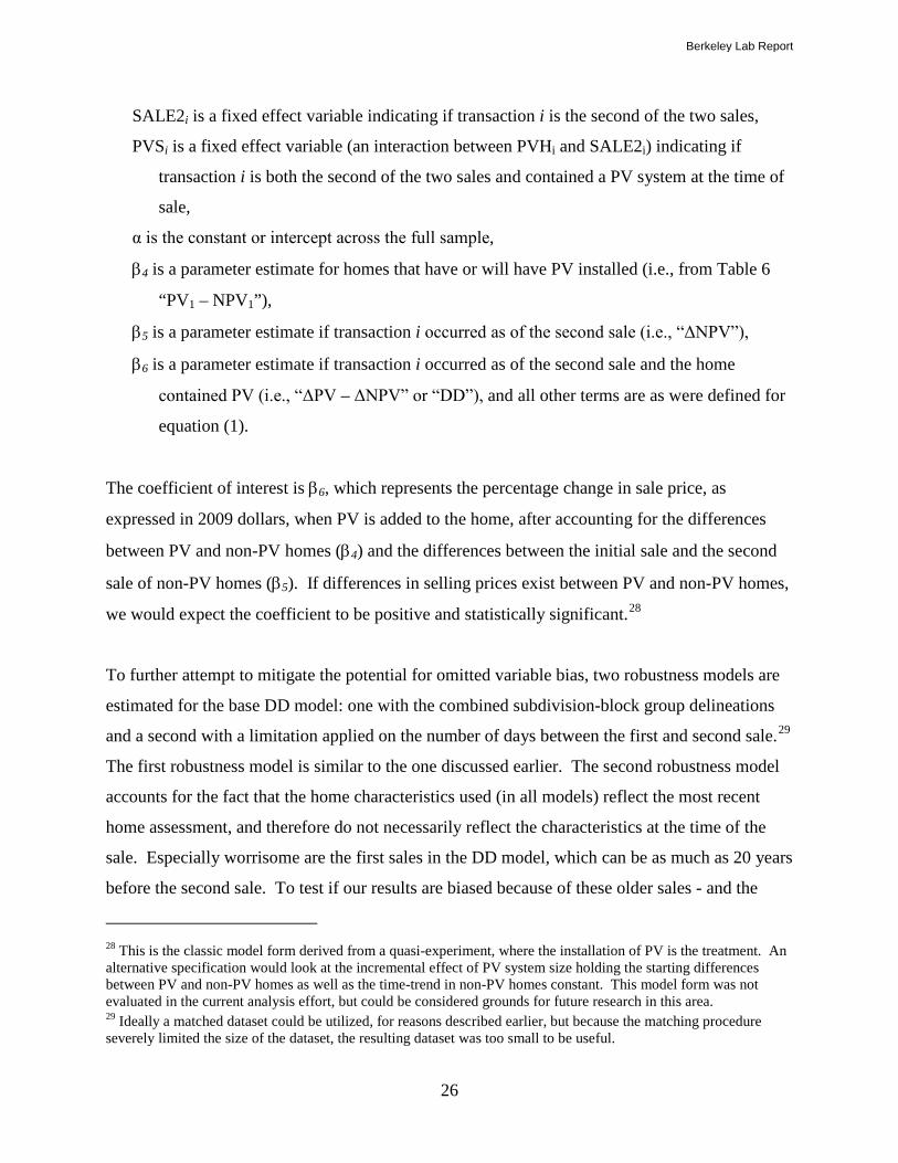
26

SALE2i is a fixed effect variable indicating if transaction i is the second of the two sales,

PVSi is a fixed effect variable (an interaction between PVHi and SALE2i) indicating if

transaction i is both the second of the two sales and contained a PV system at the time of

sale,

α is the constant or intercept across the full sample,

β4 is a parameter estimate for homes that have or will have PV installed (i.e., from Table 6

“PV1 – NPV1”),

β5 is a parameter estimate if transaction i occurred as of the second sale (i.e., “ΔNPV”),

β6 is a parameter estimate if transaction i occurred as of the second sale and the home

contained PV (i.e., “ΔPV – ΔNPV” or “DD”), and all other terms are as were defined for

equation (1).

The coefficient of interest is β6, which represents the percentage change in sale price, as

expressed in 2009 dollars, when PV is added to the home, after accounting for the differences

between PV and non-PV homes (β4) and the differences between the initial sale and the second

sale of non-PV homes (β5). If differences in selling prices exist between PV and non-PV homes,

we would expect the coefficient to be positive and statistically significant.28

To further attempt to mitigate the potential for omitted variable bias, two robustness models are

estimated for the base DD model: one with the combined subdivision-block group delineations

and a second with a limitation applied on the number of days between the first and second sale.29

28 This is the classic model form derived from a quasi-experiment, where the installation of PV is the treatment. An alternative specification would look at the incremental effect of PV system size holding the starting differences between PV and non-PV homes as well as the time-trend in non-PV homes constant. This model form was not evaluated in the current analysis effort, but could be considered grounds for future research in this area.

The first robustness model is similar to the one discussed earlier. The second robustness model

accounts for the fact that the home characteristics used (in all models) reflect the most recent

home assessment, and therefore do not necessarily reflect the characteristics at the time of the

sale. Especially worrisome are the first sales in the DD model, which can be as much as 20 years

before the second sale. To test if our results are biased because of these older sales - and the

29 Ideally a matched dataset could be utilized, for reasons described earlier, but because the matching procedure severely limited the size of the dataset, the resulting dataset was too small to be useful.

Berkeley Lab Report

27

large periods between sales - an additional data screen is applied in which the difference between

the two sale dates is limited to five years.30

3.5. Age of the PV System for Existing Homes Hedonic Models

The age of the PV system at the time of home sale could affect the sales price premium for

existing homes (PV systems on new homes are, by definition, also new). This might occur

because older PV systems have a shorter expected remaining life and may become somewhat

less efficient with age (and therefore deliver a lower net present value of bill savings), but also

because older PV systems will have generated more energy bill savings for the home seller and

the seller may therefore more-willingly accept a lower price. Together, these factors suggest that

premiums for older PV systems on existing homes would be expected to be lower than for newer

systems. In order to test this directly the following base model is estimated:

( ) ( ) ( ) ( )1 2 3 4ln( )itk t k i i i i itka

P T N X PV SIZE AGEα β β β β ε= + + + + ⋅ ⋅ +∑ (4)

where

AGEi is a categorical variable for three groups of PV system age as of the time of sale of the

home: 1) less than or equal to one year old; 2) between 2 and 4 years old; and, 3) five or

more years old.

Therefore, β4 is a vector of parameter estimates for the percentage change in sales price for each

additional kW added to a PV system for each of the three PV system age groups, and all other

terms are as are defined for equation (2). The assumption is that the coefficients for β4 will be

decreasing - indicating they are valued less - as the age of the PV systems decrease. The sample

used for this model is the same as for the existing home model defined previously.

Additionally, two sets of robustness models are explored, one using the coarsened exact matched

dataset and the other using the combined subdivision-block group delineations, to test the

robustness of the results for selection and omitted variable bias, respectively.

30 As was discussed earlier, a screen for this eventuality (using adjaar) is incorporated in our data cleaning. This test therefore serves as an additional check of robustness of the results.

Berkeley Lab Report

28

3.6. Returns to Scale Hedonic Models

As discussed earlier, it is not unreasonable to expect that any increases in the selling prices of PV

homes may be non-linear with PV system size. In equation (2), it was assumed that estimated

price differences were based on a continuous linear relationship with the size of the system. To

explore the possibility of a non-linear relationship among the full sample of homes in the dataset,

the following model is estimated:31

( ) ( ) ( ) ( )1 2 3 4 5ln( ) ( )itk t k i i i i i i itka

P T N X PV SIZE PV SIZE SIZEα β β β β β ε= + + + + ⋅ + ⋅ ⋅ +∑

(5)

where

β5 is a parameter estimate for the percentage change in sales price for each additional kW

added to a PV system squared, and all other terms are as are defined for equation (2).

A negative statistically significant coefficient (β5) would indicate decreasing returns to scale for

larger PV systems, while a positive coefficient would indicate the opposite.

Somewhat analogously, as was discussed previously, premiums for PV systems may be related

to the size of the home.32

( ) ( ) ( ) ( )1 2 3 4 5

6

ln( ) ( )

( )

itk t k i i i ia

i i i itk

P T N X SQFT PV SIZE

PV SIZE SQFT

α β β β β β

β ε

= + + + + + ⋅ +

⋅ ⋅ +

∑

To test this directly using the full dataset, the following model is

estimated:

(6)

where

SQFTi is a continuous variable for the number of square feet for the home in transaction i,33

β4 is a parameter estimate for the percentage change in sale price for each additional 1000

square feet added to the home,

31 Neither this nor the following model is coupled with robustness models in this paper. 32 PV system size is also somewhat correlated with house size as a result of the tendency for increasing energy use and larger roof areas on larger homes. If this correlation was particularly strong then coefficient estimates could be imprecise. The correlation between PV house size and PV system size in the full sample of our data, however, is rather weak, at only 0.14. Clearly, many factors other than house size impact the sizing of PV systems. 33 In all of the previous models the number of square feet is contained in the vector of characteristics represented by Xi, but in this model it is separated out for clarity.

Berkeley Lab Report

29

β5 is a parameter estimate for the percentage change in sale price for each additional kW

added to a PV system,

β6 is a parameter estimate for the percentage change in sale price for each additional 1000

square feet added to PV homes, assuming the size of the PV system does not change, and

all other terms are as were defined for equation (2).

A negative statistically significant coefficient for β6 would indicate decreasing returns to scale

for PV systems as homes increase in size. Alternatively, a positive and statistically significant

coefficient would indicate increasing returns to scale for PV systems installed on larger homes.

Berkeley Lab Report

30

3.7. Model Summary

To summarize, the entire set of 21 estimated models discussed herein is shown in Table 7. The

following definitions of terms, all of which were discussed earlier, are relevant for interpreting

the models listed in the table, and therefore are briefly reviewed again. All “base” models are

coupled with a set of “robustness” models (as noted by a capital “R” in the model number). The

“Other” (returns to scale) models are presented alone. Models 1 - 4 and 6 - 8 use the hedonic

pricing model, whereas Model 5 is based on the difference-in-difference (DD) model. “Fixed”

(versus “continuous”) means that the PV variable is entered into the regression as a zero-one

dichotomous variable (for Models 1-1Rb and 5-5Rb), whereas “continuous” (for all other

models) means that the model estimates the impact of an increase in PV system size on

residential selling prices. Base Models 1, 2, 7 and 8 use the full dataset, while Models 4 and 6

are restricted to existing homes, Model 3 to new homes, and Model 5 to the repeat sales dataset.

The “matched” models use the smaller dataset of coarsened exact matched (PV and non-PV)

homes. “Base” models estimate neighborhood fixed effects at the census block group level,

whereas the “subdivision” models estimate neighborhood fixed effects at the combined

subdivision-block group level.

Table 7: Summary of Models

Model Number Model Name

Base Model

Robustness Model

Other Models Dataset

Neighborhood Fixed Effects

1 Fixed - Base X Full Block Group1Ra Fixed - Matched X Full Matched Block Group1Rb Fixed - Subdivision X Full Subdivision/Block Group

2 Continuous - Base X Full Block Group2Ra Continuous - Matched X Full Matched Block Group2Rb Continuous - Subdivision X Full Subdivision/Block Group2Rc Continuous - PV Only X PV Only Block Group

3 New Homes - Base X New Block Group3Ra New - Matched X New - Matched Block Group3Rb New - Subdivision X New Subdivision/Block Group

4 Existing Homes - Base X Existing Block Group4Ra Existing - Matched X Existing - Matched Block Group4Rb Existing - Subdivision X Existing Subdivision/Block Group

5 Difference-in-Difference (DD) - Base X Repeat Sales Block Group5Ra Difference-in-Difference (DD) - Subdivision X Repeat Sales Subdivision/Block Group5Rb Difference-in-Difference (DD) - Sddif < 5 Years X Repeat Sales w/ sddif < 5 Block Group

6 Age of System - Base X Existing Block Group6Ra Age of System - Matched X Existing - Matched Block Group6Rb Age of System - Subdivision X Existing Subdivision/Block Group

7 Returns to Scale - Size X Full Block Group8 Returns to Scale - Square Feet X Full Block Group

Berkeley Lab Report

31

4. Estimation Results

Estimation results for all 21 models (as defined in Table 7) are presented in Tables 8-11, with the

salient results on the impacts of PV on homes sales prices summarized in Figures 2-4.34, 35 The

adjusted R2 for all models is high, ranging from 0.93 to 0.95, which is notable because the

dataset spanned a period of unusual volatility in the housing market. The model performance

reflects, in part, the ability of the inflation index and temporal fixed effects variables to

adequately control for market conditions.36

Moreover, the sign and magnitude of the home and site control variables are consistent with a

priori expectations, are largely stable across all models, and are statistically significant at the 1%

level in most models.37

34 For simplicity, this paper does not present the results for the quarter and block group (nor combined subdivision-block group) fixed effects, which consist of more than 900 coefficients. These are available upon request from the authors.

Each additional 1000 square feet of living area added to a home is

estimated to add between 19% and 26% to its value, while the first acre adds approximately 40%

to its value with each additional acre adding approximately 1.5%. For each year a home ages, it

is estimated that approximately 0.2% of its value is lost, yet at 60 years, age becomes an asset

with homes older than that estimated to garner premiums for each additional year in age. Finally,

for each additional 100 feet above the median elevation of the other homes in the block group, a

home’s value is estimated to increase by approximately 0.3%. These results can be benchmarked

to other research. Specifically, Sirmans et al. (2005a; 2005b) conducted a meta-analysis of 64

hedonic pricing studies carried out in multiple locations in the U.S. during multiple time periods,

and investigated similar characteristics as included in the models presented here, except for

relative elevation. As a group, each of the home and site characteristic estimates in the present

35 All models were estimated with Stata SE Version 11.1 using the “areg” procedure with White’s correction for standard errors (White, 1980). It should also be noted that all Durbin-Watson (Durbin and Watson, 1951) test statistics were within the acceptable range (Gujarati, 2003), there was little multicollinearity associated with the variables of interest, and all results were robust to the removal of any cases with a Cook’s Distance greater than 4/n (Cook, 1977) and/or standardized residuals greater than four. 36 As mentioned in footnote 22, a variety of approaches were tested to control for market conditions, such as spatial temporal fixed effects (e.g., census block / year quarter) both with and without adjusted sale prices. The models presented here were the most parsimonious. As importantly, the results were robust to the various specifications, which, in turn, provides additional confidence that the effects presented are not biased by the fluctuating market conditions that have impacted the housing market for some years. 37 In some models, where there is little variation between the cases on the covariate (e.g., acres), the results are non-significant at the 10% level.

Berkeley Lab Report

32

study differ from the mean Sirmans et al. estimates by no more than one half of one standard

deviation.

In summary, these results suggest that the hedonic and repeat sales models estimated here are

effectively capturing many of the drivers to home sales prices in California, and therefore

increasing confidence that those same models can be used to accurately capture any PV effects

that may exist.

4.1. Fixed and Continuous Effect Hedonic Model Results

The results from the base hedonic models (equations 1 and 2) are shown in Table 8 as Models 1

and 2, respectively. These models estimate the differences across the full dataset between PV and

non-PV homes, with Model 1 estimating this difference as a fixed effect, and Model 2 estimating

the difference as a continuous effect for each additional kilowatt (kW) of PV added. Also shown

in the table are the results from the robustness tests using the coarsened exact matching

procedure and the combined subdivision-block group delineations, as shown as Models 1Ra and

1Rb for PV fixed effect models and Models 2Ra and 2Rb for continuous effect variables.

Finally, the model that derives marginal impact estimates from only

PV homes is shown in the

table as Model 2Rc.

Across all seven of these models (Models 1 – 2Rc), regardless of the specification, the variables

of interest of PV and SIZE are positive and significant at the 10% level, with six out of seven

estimates being significant at the 1% level. Where a PV fixed effect is estimated, the coefficient

can be interpreted as the percentage increase in the sales price of a PV home over the mean non-

PV home sales price in 2009 dollars based on an average sized PV system. By dividing the

monetary value of this increase by the number of watts for the average sized system, this

premium can be converted to 2009 dollars per watt ($/watt). For example, for base Model 1,

multiplying the mean non-PV house value of $480,862 by 0.036 and dividing by 3120 watts,

yields a premium of $5.5/watt (see bottom of Table 8). Where SIZE, a continuous PV effect, is

used, the coefficients reflect the percentage increase in selling prices in 2009 dollars for each

additional kW added to the PV system. Therefore, to convert the SIZE coefficient to $/watt, the

mean house value for non-PV homes is multiplied by the coefficient and divided by 1000. For

Berkeley Lab Report

33

example, for base Model 2, $480,862 is multiplied by 0.012 and divided by 1000, resulting in an

estimate of $5.8/watt.38

As summarized in Figure 2, these base model results for the impact of PV on residential selling

prices are consistent with those estimated after controlling for subdivision fixed effects

($5.4/watt and $5.6/watt for fixed and continuous effects, respectively), differing by no more

than $0.2/watt. On the other hand, the estimated PV premiums derived from the coarsened exact

matched dataset are noticeably smaller, decreasing by 20 to 30%, and ranging from $3.9/watt to

$4.8/watt for fixed and continuous effects, respectively. Alternatively, the PV only Model 2Rc

estimates a higher $/watt continuous effect of $6.4/watt, although that estimate is statistically

significant at a lower 10% level. This estimate, because it is derived from PV homes only,

corroborates that any changes to the home that are coincident with the installation of the PV (e.g.,

energy efficient upgrades) are not influencing results dramatically.

Figure 2: Fixed and Continuous Effect Base Model Results with Robustness Tests

38 To be exact, the conversion is a bit more complicated. For example, for the fixed effect model the conversion is actually (EXP(LN(480,862)+0.036)-480,862)/3.12/1000, but the differences are de minimis, and therefore are not used herein.

$5.5 $5.8 $5.4 $5.6 $3.9 $4.8 $6.4 $0

$1

$2

$3

$4

$5

$6

$7

$8

$9

$10

Fixed Effect Hedonic Model

Continuous Effect Hedonic Model

Estim

ated

Ave

rage

Sal

e Pr

ice

Prem

ium

Fo

r PV

Hom

es (

in $

/Wat

t DC)

Base Models (n = 70425 non-PV, 1894 PV)Subdivision Robustness Models (n = 70425 non-PV, 1894 PV)Matched Robustness Models (n = 11864 non-PV, 1465 PV)PV Only Robustness Model (n = 0 non-PV, 1192 PV)

Note: Error bars represent the 90% confidence intervals for the underlying sale price premium (% change in sale price) and do not include variation in either the mean sale price or mean system size, both of which are used to calculate the $/watt premium.

Berkeley Lab Report

34

Though results among these seven models differ to some degree, the results are consistent in

finding a premium for PV homes over non-PV homes in California, which varies from $3.9 to

$6.4/watt on average, depending on the model specification. These sale price premiums are very

much in line with, if not slightly above, the historical mean net installed costs (i.e., the average

installed cost of a system, after deducting available state and federal incentives) of residential PV

systems in California of approximately $5/watt from 2001 through 2009 (Barbose et al., 2010),

which, as discussed earlier, may be reasonable given that both buyers and sellers might use this

cost as a partial basis to value a home.39

Additionally, the one other hedonic analysis of PV selling price premiums (which used

reasonably similar models as those employed here but a different dataset, concentrating only on

homes in the San Diego metropolitan area) found a similar result (Dastrop et al., 2010). In their

analysis of 279 homes that sold with PV systems installed in San Diego (our model only

contained 35 homes from this area40 Table 5 – See ), Dastrop et al. estimated an average increase

in selling price of $14,069, which, when divided by their mean PV system size of 3.2 kW,

implies an effect of $4.4/watt.41

39 Although not investigated here, one possible reason for sales price premiums that are above net installed costs is that buyers of PV homes may in some cases price in the opportunity cost of avoiding having to do the PV installation themselves, which might be perceived as complex. Moreover, a PV system installation that occurs after the purchase of the home would likely be financed outside the first mortgage and would therefore loose valuable finance and tax benefits, thereby making the purchase of a PV home potentially more attractive that installing a PV system later, even if at the same cost.

40 Though we identified a higher number of PV homes that sold in the San Diego metropolitan area in our dataset, the home and site characteristics provided to us from the real estate data provider did not contain information on the year of the sale and therefore were not usable for the purpose of our analysis. 41 In a different model, Dastrop et al. (2010) estimated an effect size of $2.4/watt but, for reasons not addressed here, this estimate is not believed to be as robust.

Berkeley Lab Report

35

Table 8: Fixed and Continuous Base Hedonic Model Results with Robustness Tests

4.2. New and Existing Home Model Results

Turning from the full dataset to one specific to the home type, we estimate continuous effects

models for new and existing homes (see equation (2)). These results are shown in Table 9, with

Model 3 the base model for new homes and Model 4 the base model for existing homes. Also

Base Robustness Robustness Base Robustness Robustness RobustnessMatched Subdivision Matched Subdivision PV Only

Model 1 Model 1Ra Model 1Rb Model 2 Model 2Ra Model 2Rb Model 2Rcpv 0.036*** 0.024*** 0.035***

(0.005) (0.006) (0.005)size 0.012*** 0.010*** 0.012*** 0.013*

(0.002) (0.002) (0.001) (0.008)sqft_1000 0.253*** 0.205*** 0.250*** 0.253*** 0.205*** 0.250*** 0.224***

(0.001) (0.006) (0.001) (0.001) (0.006) (0.001) (0.010)lt1acre 0.417*** 0.514*** 0.414*** 0.416*** 0.510*** 0.413*** 0.441***

(0.009) (0.040) (0.010) (0.009) (0.040) (0.010) (0.066)acre 0.016*** 0.013 0.015*** 0.016*** 0.013 0.015*** -0.002

(0.002) (0.011) (0.003) (0.002) (0.010) (0.003) (0.012)ages2 -0.004*** -0.006*** -0.004*** -0.004*** -0.006*** -0.004*** -0.008***

(0.0002) (0.0012) (0.0002) (0.0002) (0.0012) (0.0002) (0.0030)ages2sqr 0.00003*** 0.00004*** 0.00003*** 0.00003*** 0.00004*** 0.00003*** 0.00004***

(0.000003) (0.000012) (0.000003) (0.000003) (0.000012) (0.000003) (0.000033)bgre_100 0.003*** 0.015*** 0.003*** 0.003*** 0.015*** 0.003*** 0.013***

(0.001) (0.004) (0.001) (0.001) (0.004) (0.001) (0.005)intercept 12.703*** 12.961*** 12.710*** 12.702*** 12.957*** 12.710*** 12.842***

(0.010) (0.044) (0.012) (0.010) (0.043) (0.012) (0.073)Numbers in parenthesis are standard errors, *** p<0.01, ** p<0.05, * p<0.1Results for subdivision, block group, and quarterly fixed effect variables are not reported here, but are available upon request from the authors

Total n 72,319 13,329 72,319 72,319 13,329 72,319 1,192

Adjusted R2 0.93 0.95 0.94 0.93 0.95 0.94 0.93n (pv homes) 1,894 1,465 1,894 1,894 1,465 1,894 1,192Mean non-pv asp2 480,862$ 480,533$ 480,862$ 480,862$ 480,533$ 480,862$ 475,811$ Mean size (kW) 3.1 3.0 3.1 3.1 3.0 3.1 2.7Estimated $/Watt 5.5$ 3.9$ 5.4$ 5.8$ 4.8$ 5.6$ 6.4$

ContinuousFixed

PV Only Model Notes: Mean non-pv asp2 amount shown is actually the mean PV asp2. Sample is limited to blockgroups with more than one PV home

Berkeley Lab Report

36

shown are the results from the robustness tests using the coarsened exact matching procedure and

the combined subdivision-block group delineations, as Models 3Ra and 3Rb, respectively, for

new homes, and as Models 4Ra and 4Rb, respectively, for existing homes.

The coefficient of interest, SIZE, is statistically significant at or below the 10% level in all of the

new home models and at the 1% level in all of the existing home models. Estimates for the

average $/watt increase in selling prices as a result of PV systems (as summarized in Figure 3,

which also includes the results presented earlier for all homes, Models 2, 2Ra, and 2Rb) for new

homes are quite stable, ranging from $2.3 to $2.6/watt. In comparison, for PV sold with existing

homes, not only are the selling price impacts found to be higher, but their range across the three

models is somewhat greater, ranging from $ 6.4 to $7.7/watt.

Figure 3: New and Existing Home Base Model Results with Robustness Tests

Though the reasons for the apparent discrepancy in selling price impacts between new and

existing homes are unclear, and warrant future research, they might be explained, in part, by the

difference in average net installed costs, which, from 2007 to 2009, were approximately

$5.2/watt for existing homes and $4.2/watt for new homes in California (derived from the dataset

used for Barbose et al., 2010). The gap in net installed costs between new and existing homes is

$5.8 $5.6 $4.8 $2.3 $2.6 $2.6 $7.7 $6.5 $6.4 $0

$1

$2

$3

$4

$5

$6

$7

$8

$9

$10

$11

$12

Base (Continuous) Hedonic Models

Subdivision Robustness Hedonic Models

Matched Robustness Hedonic Models

Estim

ated

Ave

rage

Sal

e Pr

ice P

rem

ium

Fo

r PV

Hom

es (i

n $/

Wat

t DC)

All Homes (Non-PV & PV n in Base & Subdivision Models: 70425, 1894; in Matched Models: 11864, 1465)New Homes (Non-PV & PV n in Base & Subdivision Models: 26938, 935; in Matched Models: 7266, 802)Existing Homes (Non-PV & PV n in Base & Subdivision Models: 43487, 897; in Matched Models: 4269, 618)


Berkeley Lab Report

37

not wide enough to fully account for these findings, however, with the model estimates for PV

selling price premiums below the average net installed costs for new homes and above the

average net installed costs for existing homes.42

Several alternative explanations for the disparity between new and existing home premiums exist.

As discussed previously, there is evidence that builders of new homes might discount premiums

for PV if, in exchange, PV systems provide other benefits for new home developers, such as

greater product differentiation and increased the sales velocity, thus decreasing overall carrying

costs (Dakin et al., 2008; SunPower, 2008). Further, sellers of new homes with PV might be

reluctant to aggressively increase home sale prices for installed PV systems because of the

burgeoning state of the market for PV homes and concern that more aggressive pricing could

even slow home sales. Additionally, because many builders of new homes found that offering PV

as an option, rather than a standard feature, posed a set of difficulties (Farhar et al., 2004b; Dakin

et al., 2008), it has been relatively common in past years for PV to be sold as a standard feature

on homes (Dakin et al., 2008). This potentially affects the valuation of PV systems for two

reasons. First, because sales agents for the new PV homes have sometimes been found to either

not be well versed in the specifics of PV and felt that selling a PV system was a new sales pitch

(Farhar et al., 2004b) or to have combined the discussion of PV with a set of other energy

features (Dakin et al., 2008), up-selling the full value of the PV system as a standard product

feature might not have been possible. Secondly, the average sales price of new homes in our

dataset is lower than the average sales price of existing homes: to the extent that PV is

considered a luxury good, it may be somewhat less-highly valued for the buyers of these homes.

These downward influences for new homes are potentially contrasted with analogous upward

influences for existing homes. Related, buyers of existing homes with PV may - to a greater

degree than buyers of the less expensive new homes in our sample - be self selected towards

those who place particular value on a PV home, and therefore value the addition more. Finally,

in contrast to new home sellers, who might not be familiar with the intricacies and benefits of the 42 A small number of “affordable homes” (n = 7) are included in the new PV homes subset, which, as a group, appear to have a slight downward yet inconsequential effect on the overall sales premium results, and therefore were not investigated further herein. If the number of affordable homes with PV was significant in future research, those effects would best be controlled for directly.

Berkeley Lab Report

38

PV system, existing home sellers are likely to be very familiar with the particulars of the system

and its benefits, and therefore might be able to “up-sell” it more effectively.

These possible influences, in combination, may explain the difference in average PV premium

between new and existing homes. The present analysis did not seek to disentangle or evaluate

these specific drivers, however, leaving that important effort for future research.

Table 9: New and Existing Home Base Hedonic Model Results with Robustness Tests

Base Robustness Robustness Base Robustnes RobustnessMatched Subdivision Matched Subdivision

Model 3 Model 3Ra Model 3Rb Model 4 Model 4Ra Model 4Rbsize 0.006* 0.006* 0.006** 0.014*** 0.011*** 0.012***

(0.003) (0.003) (0.003) (0.002) (0.002) (0.002)sqft_1000 0.247*** 0.190*** 0.250*** 0.256*** 0.238*** 0.251***

(0.002) (0.006) (0.002) (0.002) (0.015) (0.002)lt1acre 0.536*** 0.279*** 0.517*** 0.373*** 0.426*** 0.376***

(0.019) (0.073) (0.024) (0.010) (0.046) (0.012)acre -0.007 0.338*** -0.009* 0.019*** 0.011 0.017***

(0.005) (0.027) (0.005) (0.002) (0.011) (0.003)ages2 -0.010 0.081*** -0.010* -0.005*** -0.006*** -0.005***

(0.006) (0.017) (0.006) (0.000) (0.002) (0.000)ages2sqr 0.00768*** -0.02443*** 0.00715*** 0.00004*** 0.00004*** 0.00004***

(0.001676) (0.004407) (0.001604) (0.000003) (0.000014) (0.000004)bgre_100 0.008*** 0.027*** 0.007*** 0.002 -0.002 0.002

(0.001) (0.003) (0.001) (0.001) (0.009) (0.001)intercept 12.651*** 12.585*** 12.627*** 12.820*** 13.023*** 12.833***

(0.022) (0.066) (0.025) (0.013) (0.077) (0.014)Numbers in parenthesis are standard errors, *** p<0.01, ** p<0.05, * p<0.1Results for subdivision, block group, and quarterly fixed effect variables are not reported here, but are available upon request from the authors

Total n 27,873 8,068 27,873 44,384 4,887 44,384

Adjusted R2 0.94 0.94 0.94 0.93 0.95 0.94n (pv homes) 935 802 935 897 618 897Mean non-pv asp2 397,265$ 399,162$ 397,265$ 532,645$ 590,428$ 532,645$ Mean size (kW) 2.5 2.4 2.5 3.8 3.7 3.8Estimated $/Watt 2.3$ 2.6$ 2.6$ 7.7$ 6.4$ 6.5$

Existing HomesNew Homes

Berkeley Lab Report

39

4.2.1. Difference-in-Difference Model Results

Delving deeper into PV system impacts on existing homes, Table 10 (and Figure 4) shows the

results of the base Difference-in-Difference Model 5 as well as results from the two robustness

tests (all of which can be compared to Models 4, 4Ra, and 4rb above, as is done in Figure 4). As

a reminder, one robustness model limited the differences in sales dates between the first and

second sales to five years (Model 5Rb), and the other robustness model used the combined

subdivision-block group delineations as fixed effects variables (Model 5Rc). The variables of

interest are PVH, SALE2 and especially PVS.

PVH estimates the difference in the first sale prices of homes that will have PV installed (as of

the second sale date) relative to non-PV homes. The three models are consistent in their

estimates, showing approximately a 2% premium for “future” PV homes, though only two of

these estimates are statistically significant, and then only at the 10% level. Regardless, this

finding suggests that PV homes tend to sell for somewhat more even before the installation of

PV, presumably as a result of other amenities that are correlated with the (ultimate) installation

of PV (such as, potentially, energy efficiency features). SALE2 estimates the price appreciation

trend between the first and second sales for all homes. The coefficient for this variable is

significant at the 1% level, and is fairly stable across the models, indicating a clear general trend

of price increases, over and above inflation adjustments, of approximately 2% to 2.5% between

the first and second sales.

Finally, and most importantly, homes with PV systems installed on them as of the second sale -

after controlling for any inherent differences in first sale prices (PVH) and any trend between the

first and second sales (SALE2) - show statistically significant sale price premiums of

approximately 5 to 6%. These premiums equate to an increase in selling prices of approximately

$6/watt for existing homes, closely reflecting the results presented earlier for the hedonic models

in Table 9 and Figure 3. For comparison purposes, both sets of results are presented in Figure 4.

The premium for existing PV homes as estimated in the DD Models 5, 5Ra, and 5Rb and both

robustness tests for the hedonic model (using the “matched” and “subdivision” datasets, Models

4Ra and 4Rb respectively) are consistently between $6 and $6.5/watt and are in line with –

Berkeley Lab Report

40

though slightly higher than - the mean net installed costs of PV on existing homes in California

of approximately $5.2/watt from 2007 through 2009. The base hedonic existing home model, on

the other hand, estimates a higher premium of $7.7/watt. One possible explanation for this

inconsistency is that the two robustness tests for the hedonic model and the various difference-in-

difference models are less likely to be influenced by either selection or omitted variable bias than

the base hedonic model. Regardless of the absolute magnitude, a sizable premium for existing

PV homes over that garnered by new PV homes is clearly evident in these and the earlier results.

Figure 4: Existing Home Hedonic and Difference-in-Difference Model Results with

Robustness Tests

$7.7 $6.2 $6.5 $6.0 $6.4 $6.3 $0$1$2$3$4$5$6$7$8$9

$10$11$12$13$14$15

Existing Homes Hedonic Model

Existing Homes Difference-in-Difference Model

Estim

ated

Ave

rage

Sal

e Pr

ice

Prem

ium

Fo

r PV

Hom

es (i

n $/

Wat

t DC)

Base Models (Non-PV & PV n: Existing-43487, 897; DD-27919, 394)Subdivision Robustness Models (Non-PV & PV n: Existing-43487, 897; DD-27919, 394)Matched Robustness Model (Non-PV & PV n: Existing-4269, 618)SDDif < 5 Years Robustness Model (Non-PV & PV n: DD-19106, 159)


Berkeley Lab Report

41

Table 10: Difference-in-Difference Model Results

4.3. Age of PV System for Existing Home Hedonic Model Results

To this point, the marginal impacts to selling prices of each additional kW of PV added to

existing homes have been estimated using the full dataset of existing homes, which has produced

an average effect, regardless of the age of the PV system. As discussed previously, it is

Base Robustness RobustnessSubdivision Sddif < 5

Model 5 Model 5Ra Model 5Rbpvh 0.022* 0.024 0.022*

(0.013) (0.021) (0.012)sale2 0.023*** 0.026*** 0.019***

(0.002) (0.002) (0.002)pvs 0.051*** 0.061** 0.049***

(0.017) (0.027) (0.015)sqft_1000 0.255*** 0.256*** 0.251***

(0.002) (0.002) (0.002)lt1acre 0.374*** 0.385*** 0.377***

(0.011) (0.013) (0.012)acre 0.012*** 0.009** 0.011***

(0.003) (0.004) (0.003)age -0.005*** -0.005*** -0.005***

(0.0002) (0.0003) (0.0003)agesqr 0.00004*** 0.00004*** 0.00004***

(0.000003) (0.000003) (0.000003)bgre_100 0.002* 0.000 0.001

(0.001) (0.001) (0.001)intercept 12.677*** 12.594*** 12.694***

(0.013) (0.015) (0.014)

Total n 28,313 19,265 28,313

Adjusted R2 0.93 0.94 0.94n (pv homes) 394 159 394Mean non-pv asp2 488,127$ 450,223$ 488,127$ Mean size (kW) 4.0 4.3 4.0Estimated $/Watt 6.2$ 6.3$ 6.0$

Difference-in-Difference

Numbers in parenthesis are standard errors. *** p<0.01, ** p<0.05, * p<0.1. Results for subdivision, block group, and quarterly fixed effect variables are not reported here, but are available upon request from the authors

Berkeley Lab Report

42

conceivable that older PV systems would garner lower premiums than newer, similarly sized

systems. To test this directly, a base model is constructed - see equation (4) - that estimates the

marginal impacts for three age groups of PV systems: no more than one year old at the time of

sale; between two and four years old; and five or more years old. Results from this model as

well as two robustness tests, using the coarsened exact matching procedure and the combined

subdivision-block group delineations, are shown in Table 11 as Models 6, 6Ra, and 6Rb,

respectively.

Each model finds statistically significant differences between PV and non-PV homes for each

age group, and more importantly, premium estimates for newer PV systems are - as expected -

larger than those for older PV systems and are monotonically ordered between groups, providing

some evidence that older systems are being discounted by the buyers and sellers of PV homes.

Specifically, the three models estimate an average premium for PV systems that are one year or

less in age of $8.3-9.3/watt, whereas those same models estimate an average premium of $4.1-

6.1/W for systems that are five or more years old.

4.4. Returns to Scale Hedonic Model Results

In the previous modeling, the marginal impacts to selling prices of each additional kW of PV in

the continuous models have been estimated using a linear relationship. To test whether a non-

linear relationship may be a better fit, a SIZE squared term is added to the model as shown in

equation (5). Similarly, decreasing or increasing returns to scale might be related to other house

characteristics, such as the size of the home (i.e., square feet). This hypothesis is explored using

equation (6). Both model results are shown in Table 11 as Model 7 and 8, respectively.

Both models find small and non-statistically significant relationships between their interacted

variables, indicating a lack of compelling evidence of a non-linear relationship between PV

system size and selling price in the dataset, and a lack of compelling evidence that the linear

relationship is affected by the size of the home. As such, the impact of PV systems on residential

selling prices appears to be well approximated by a simple linear relationship, while the size of

the home is not found to impact the PV sales price premium. In combination, these results seem

to suggest that while California’s tiered rate structures may lead to energy bill savings from PV

Berkeley Lab Report

43

investments that vary non-linearly with PV system size and also vary by home size, those same

rate structures have not – to this point – led to any clear impact on the PV premium garnered at

the time of home sale. Similarly, though larger PV systems may be installed at a discount to

smaller ones on a $/watt basis, and though any marginal green cachet that exists may diminish

with system size, those possible influences are not apparent in the results presented here.

Berkeley Lab Report

44

Table 11: Age of PV System and Return to Scale Hedonic Model Results

Base Robustness Robustness Size Square FeetMatched Subdivision

Model 6 Model 6Ra Model 6Rb Model 7 Model 8size*1 year old 0.016*** 0.016*** 0.013***

(-0.004) (-0.005) (-0.004)size*2-4 years old 0.015*** 0.010*** 0.013***

(-0.002) (-0.003) (-0.002)size*5+ years old 0.012*** 0.008** 0.008**

(-0.003) (-0.004) (-0.003)size 0.008** 0.021***

(0.003) (0.006)sizesqr 0.001

(0.001)size*sqft_1000 -0.003

(0.002)sqft_1000 0.256*** 0.238*** 0.251*** 0.253*** 0.253***

(0.002) (0.015) (0.002) (0.001) (0.001)lt1acre 0.373*** 0.426*** 0.376*** 0.416*** 0.416***

(0.010) (0.046) (0.012) (0.009) (0.009)acre 0.019*** 0.010*** 0.017*** 0.016*** 0.016***

(0.002) (0.011) (0.003) (0.002) (0.002)ages2 -0.005*** -0.006*** -0.005*** -0.004*** -0.004***

(0.000) (0.002) (0.000) (0.000) (0.000)ages2sqr 0.000*** 0.000*** 0.000*** 0.000*** 0.000***

(0.000) (0.000) (0.000) (0.000) (0.000)bgre_100 0.002*** -0.002*** 0.002*** 0.003*** 0.003***

(0.001) (0.009) (0.001) (0.001) (0.001)intercept 12.820*** 13.024*** 12.834*** 12.702*** 12.701***

(0.013) (0.078) (0.014) (0.010) (0.011)Numbers in parenthesis are standard errors. *** p<0.01, ** p<0.05, * p<0.1

Total n 44,384 4,887 44,384 72,319 72,319

Adjusted R2 0.93 0.95 0.94 0.93 0.93n (pv homes) 897 618 897 1,894 1,894Mean non-pv asp2 532,645$ 590,428$ 532,645$ 480,862$ 480,862$ Mean size (kW) 3.8 3.7 3.8 3.1 3.1Estimated $/Watt $8.3 - $6.1 $9.3 - $4.9 $7.0 - $4.1 6.3$ 6.4$

Returns to ScaleAge of PV Systems for Existing Homes

Note: $/watt estimates for Returns to Scale models include the non-statistically significant interaction coefficients and therefore should be interpreted with caution

Results for subdivision, block group, and quarterly fixed effect variables are not reported here, but are available upon request from the authors

Berkeley Lab Report

45

5. Conclusions

The market for solar PV is expanding rapidly in the U.S. Almost 100,000 PV systems have been

installed in California alone, more than 90% of which are residential. Some of those “PV homes”

have sold, yet little research exists estimating if those homes sold for significantly more than

similar non-PV homes. Therefore, one of the claimed incentives for solar homes - namely that a

portion of the initial investment into a PV system will be recouped if the home is sold – has, to

this point, been based on limited evidence. Practitioners have sometimes transferred the results

from past research focused on energy efficiency and energy bills more generally and, while

recent research has turned to PV that research has so far focused largely on smaller sets of PV

homes concentrated in certain geographic areas. Moreover, the home sales price effect of PV on

a new versus an existing home has not previously been the subject of research. Similarly

unexplored has been whether the relationship of PV system size to home sales prices is linear,

and/or is affected by either the size of the home or the age of the PV system.

This research has used a dataset of approximately 72,000 California homes, approximately 2,000

of which had PV systems installed at the time of sale, and has estimated a variety of different

hedonic and repeat sales models to directly address the questions outlined above. Moreover, an

extensive set of robustness tests were incorporated into the analysis to test and bound the

possible effects and increase the confidence of the findings by mitigating potential biases. The

research was not intended to disentangle the various individual underlying influences that might

dictate the level of the home sales price premium caused by PV, such as, energy costs savings,

the net (i.e., after applicable state and federal incentives) installed cost of the PV system, the

possible presence of a green cachet, or seller attributes. Instead, the goal was to establish

credible estimates for the aggregate PV residential sale price effect across a range of different

circumstances (e.g., new vs. existing homes, PV system age).

The research finds strong evidence that homes with PV systems in California have sold for a

premium over comparable homes without PV systems. More specifically, estimates for average

PV premiums range from approximately $3.9 to $6.4 per installed watt (DC) among a large

number of different model specifications, with most models coalescing near $5.5/watt. That

Berkeley Lab Report

46

value corresponds to a premium of approximately $17,000 for a relatively new 3,100 watt PV

system (the average size of PV systems in the study). These results are similar to the average

increase for PV homes found by Dastrop et al. (2010), which used similar methods but a

different dataset, one that focused on homes in the San Diego metropolitan area. Moreover,

these average sales price premiums appear to be comparable to the average net (i.e., after

applicable state and federal incentives) installed cost of California residential PV systems from

2001-2009 (Barbose et al., 2010) of approximately $5/watt, and homeowners with PV also

benefit from electricity cost savings after PV system installation and prior to home sale.

Although the results for the full dataset from the variety of models are quite similar, when the

dataset is split among new and existing homes, PV system premiums are found to be markedly

affected, with new homes demonstrating average premiums of $2.3-2.6/watt, while existing

homes are found to have average premiums of $6-7.7/watt. Possible reasons for this disparity

between new and existing PV homes include: differences in underlying net installation costs for

PV systems; a willingness among builders of new homes to accept a lower PV premium because

PV systems provide other benefits to the builders in the form of product differentiation, leading

to increased sales velocity and decreased carrying costs; and, lower familiarity and/or interest in

marketing PV systems separately from the other features of new homes contrasted with a likely

strong familiarity with the PV systems among existing home sellers.

The research also investigated the impact of PV system age on the sales price premium for

existing homes, finding - as would be expected - evidence that older PV systems are discounted

in the marketplace as compared to newer PV systems. Finally, evidence of returns to scale for

either larger PV systems or larger homes was investigated but not found.

In addition to benchmarking the results of this research to the limited previous literature

investigating the sales price premiums associated with PV, our results can also be compared to

previous literature investigating premiums associated with energy efficiency (EE) or, more

generally, energy cost savings. A number of those studies have converted this relationship into a

ratio representing the relative size of the home sales price premium to the annual savings

expected due to energy bill reductions. These ratios have ranged from approximately 7:1

Berkeley Lab Report

47

(Longstreth et al., 1984; Horowitz and Haeri, 1990), to 12:1 (Dinan and Miranowski, 1989), to

approximately 20:1 (Johnson and Kaserman, 1983; Nevin et al., 1999; Eichholtz et al., 2009),

and even as high as 31:1 (Nevin and Watson, 1998).

Although actual energy bill savings from PV for the sample of homes used for this research were

not available, a rough estimate is possible, allowing for a comparison to the previous results for

energy-related homes improvements and energy efficiency. Specifically, assuming that 1,425

kWh (AC) are produced per year per kW (DC) of installed PV on a home (Barbose et al., 2010;

CPUC, 2010)43

Figure 5

and that this production offsets marginal retail electricity rates that average

$0.20/kWh (AC) (Darghouth et al., 2010), each watt (DC) of installed PV can be estimated to

save $0.29 in annual energy costs. Using these assumptions, the $/watt PV premium estimates

reported earlier can be converted to sale price to annual energy savings ratios (see ).

A $3.9 to $6.4/watt premium in selling price for an average California home with PV installed

equates to a 14:1 to 22:1 sale price to energy savings ratio, respectively. For new homes, with a

$2.3-2.6/watt sale price premium, this ratio is estimated to be 8:1 or 9:1, and for existing homes,

with an overall sale price premium range of $6-7.6/watt, the ratio is estimated to range from 21:1

to 26:1. Without actual

energy bill savings, these estimates are somewhat speculative, but

nonetheless are broadly consistent with the previous research that has focused on EE-based home

energy improvements.

43 The 1,425 kWh (AC) estimate is based on a combination of a 19% capacity factor (based on AC kWh and CEC-AC kW) from CPUC (2010), and an 0.86 conversion factor between CEC-AC kW and DC kW (Barbose et al., 2010).

Berkeley Lab Report

48

Figure 5: Estimated Ratios of Sale Price Premium to Annual Energy Cost Savings

Although this research finds strong evidence that homes with PV systems in California have sold

for a premium over comparable homes without PV systems, the extrapolation of these results to

different locations or market conditions (e.g., different retail rates or net installed costs) should

be done with care.

Finally, additional questions remain that warrant further study. Perhaps most importantly,

although the dataset used for this analysis consists of almost 2,000 PV homes, the study period

was limited to sales occurring prior to mid-2009 and the dataset was limited to California.

Future research would therefore ideally include more-recent sales from a broader geographic

area to better understand any regional/national differences that may exist as well as any changes

to PV premiums that occur over time as the market for PV homes and/or the net installed cost of

PV changes. More research is also warranted on new versus existing homes to better understand

the nature and underlying drivers for the differential premium discovered in this research; in

addition to further hedonic analysis, that research could include interviewing/surveying home

builders and buyers and exploring the impact of demographic, socio-economic, and others

factors on the PV premium.

0:1

5:1

10:1

15:1

20:1

25:1

30:1

Estim

ated

Sal

e Pr

ice

Prem

ium

To

Ann

ual E

nerg

y Co

st S

avin

gs R

atio

Base Models Subdivision Models Matched ModelsPV Only Model Sddif<5 Model

All Homes New Homes Existing Homes Existing HomesHedonic Hedonic Hedonic Difference-inModels* Models Models Difference

Models *All Homes Models Include Fixed and Continuous. The following assumptions were used for this calculation: 1,425 kWh AC are

produced by each kW DC of PV. Energy cost savings equal $0.20/kWh AC. Sources: CPUC, 2010; Barbose et al., 2010.

Berkeley Lab Report

49

Additionally, future research might compare sales price premiums to actual annual home energy

cost savings, to not only to explore the sale price to annual energy cost savings ratio directly, but

also to explore if a green cachet exists over and above any sale price premiums that would be

expected from energy cost savings alone. Further, house-by-house PV system and other

information not included in the present study might be included in future studies, such as the

actual net installed costs of PV for individual households, rack-mounted or roof-integrated

distinctions as well as other elements of PV system design, the level of energy efficiency of the

home, whether the home has a solar hot water heater, whether the PV system is customer or 3rd

party owned at the time of sale, and if the homeowner can sell the green attributes the system

generates.44

44 3rd party owned PV systems would not be expected to command the same sort of premium as was discovered here. Although the level of penetration of 3rd party owners in our data was not significant (below 10%), and therefore would likely have not influenced our results in a substantive way, any future research, using more recent data, must account for their inclusion specifically.

Such research could elucidate important differences in PV premiums among

households, PV system designs and state and federal programmatic designs, as well as bolster

confidence in the magnitude of the PV premium estimated here. Finally, and more generally,

additional research could investigate the impact of PV systems on the time homes remain on the

market before sale, a factor that may be especially important for large developers and sellers of

new homes.

Berkeley Lab Report

50

References

Barbose, G., Darghouth, N. and Wiser, R. (2010) Tracking the Sun III: The Installed Cost of Photovoltaics in the U.S. From 1998-2009. Lawrence Berkeley National Laboratory, Berkeley, CA. December 2010. 54 pages. LBNL-4121E.

Black, A. (2010) Does It Pay? Figuring the Financial Value of a Solar or Wind Energy System. Solar Today

Brounen, D. and Kok, N. (2010) On the Economics of Energy Labels in the Housing Market.

. Fall/Winter 2010. pp. 26-27.

Program on Housing and Urban Policy: Working Papers Series

California Energy Commission (CEC) (2002) Consultant Report: Renewable Energy Study. The Phelps Group and ICF Consulting. Prepared for California Energy Commission (CEC). November 2001. 77 pages.

. Prepared for Institute of Business and Economic Research and Fisher Center for Real Estate and Urban Economics, University of California, Berkeley, CA. August 2010. 34 pages. W10-002.

California Public Utilities Commission (CPUC) (2010) CPUC California Solar Initiative: 2009 Impact Evaluation. Final Report. Prepared by: Itron and KEMA. Prepared for California Public Utilities Commission, Energy Division. June 2010. 632 pages.

Cook, R. D. (1977) Detection of Influential Observations in Linear Regression. Technometrics. 19(1): 15-18.

Dakin, W., Springer, D. and Kelly, B. (2008). Case Study: The Effectiveness of Zero Energy Home Strategies in the Marketplace. Presented at ACEEE Summer Study on Energy Efficiency in Buildings, Pacific Grove, California. August 17–22, 2008.

Darghouth, N., Barbose, G. and Wiser, R. (2010) The Impact of Rate Design and Net Metering on the Bill Savings from Distributed PV for Residential Customers in California. Lawrence Berkeley National Laboratory, Berkeley, CA. December 2010. 62 pages. LBNL-3276E.

Dastrop, S., Zivin, J. G., Costa, D. L. and Kahn, M. E. (2010) Understanding the Solar Home Price Premium: Electricity Generation and “Green” Social Status. Working Paper Series

Dinan, T. M. and Miranowski, J. A. (1989) Estimating the Implicit Price of Energy Efficiency Improvements in the Residential Housing Market: A Hedonic Approach. Journal of Urban Economics. 25(1): 52-67.

. Prepared for UC Center for Energy and Environmental Economics, Berkeley, CA. December 9, 2010. 29 pages. E3 WP-001.

Durbin, J. and Watson, G. S. (1951) Testing for Serial Correlation in Least-Squares Regression. Biometrika. 38(1-2): 159-178.

Berkeley Lab Report

51

Eichholtz, P., Kok, N. and Quigley, J. M. (2009) Doing Well by Doing Good? An Analysis of the Financial Performance of Green Office Buildings in the USA. University of California. Institute of Business and Economic Research. Berkeley Program on Housing and Urban Policy, Berkeley, CA. April 1, 2008. 49 pages. W08-001S.

Eichholtz, P., Kok, N. and Quigley, J. M. (2011) The Economics of Green Building. Working Paper Series

Farhar, B. and Coburn, T. (2008) A New Market Paradigm for Zero-Energy Homes: A Comparative Case Study. Environment: Science and Policy for Sustainable Development 50(1): 18-32.

Prepared for UC Center for Energy and Environmental Economics (UCE3), Berkeley, CA. January 2011. 35 pages. WP-002.

Farhar, B. and Coburn, T. C. (2006) A New Market Paradigm for Zero-Energy Homes: The Comparative San Diego Case Study. Volume 1 of 2. Prepared for National Renewable Energy Laboratory, Bolder, CO. December 2006. 413 pages. NREL/TP-550-38304-01.

Farhar, B. C., Coburn, T. C. and Murphy, M. (2004a) Comparative Analysis of Home Buyer Response to New Zero-Energy Homes. Summer Study on Energy Efficiency in Buildings, August 22-27, 2004

Farhar, B. C., Coburn, T. C. and Murphy, M. (2004b) Large-Production Home Builder Experience with Zero Energy Homes.

. Prepared for American Council for an Energy-Efficient Economy, Pacific Grove, California. Preprinted in July, 2004. NREL/CP-550-35912.

Summer Study on Energy Efficiency in Buildings, August 22-27, 2004

Freeman, A. M. (1979) Hedonic Prices, Property Values and Measuring Environmental Benefits: A Survey of the Issues. Scandinavian Journal of Economics. 81(2): 154-173.

. Prepared for American Council for an Energy-Efficient Economy, Pacific Grove, California. Preprinted in July, 2004. 15 pages. NREL/CP-550-35913.

Griffin, A., Kaufman, B. and Hamilton, S. (2009) Certified Home Performance: Assessing the Market Impacts of Third Party Certification on Residential Properties. Earth Advantage Institute. Prepared for Green Building Value Initiative Steering Committee, Portland, OR. May 29, 2009. 36 pages.

Gujarati, D. N. (2003) Basic Econometrics

Hoen, B., Wiser, R., Cappers, P., Thayer, M. and Sethi, G. (2009) The Impact of Wind Power Projects on Residential Property Values in the United States: A Multi-Site Hedonic Analysis. Lawrence Berkeley National Laboratory, Berkeley, CA. December, 2009. 146 pages. LBNL-2829E.

. McGraw-Hill/Irwin. Fourth Edition, New York. 1002 pages. ISBN 0-07-233542-4.

Horowitz, M. J. and Haeri, H. (1990) Economic Efficiency vs. Energy Efficiency: Do Model Conservation Standards Make Good Sense? Energy Economics. 12(2): 122-131.

Johnson, R. C. and Kaserman, D. L. (1983) Housing Market Capitalization of Energy-Saving Durable Good Investments. Economic Inquiry. 21: 374 - 386.

Berkeley Lab Report

52

King, G., Blackwell, M., Iacus, S. and Porro, G. (2010) Cem: Coarsened Exact Matching in Stata. Stata Journal. 9(4): 524-546.

Laquatra, J. (1986) Housing Market Capitalization of Thermal Integrity. Energy Economics. 8(3): 134-138.

Longstreth, M., Coveney, A. R. and Bowers, J. S. (1984) Conservation Characteristics among Determinants of Residential Property Value. Journal of Consumer Research. 11(1): 564-571.

Malpezzi, S. (2003) Hedonic Pricing Models: A Selective and Applied Review. Section in Housing Economics and Public Policy: Essays in Honor of Duncan Maclennan

McCabe, M. and Merry, L. (2010) Resale Market Value of Residential Solar PV. Journal of Sustainable Real Estate. Volume 2. Industry Perspectives. Retrieved March 28, 2011 from

. Wiley-Blackwell. Hoboken, NJ. pp. 67-85 of 328 pages. ISBN 978-0-632-06461-8.

http://www.costar.com/josre/industryPerspectives.htm

Nevin, R., Bender, C. and Gazan, H. (1999) More Evidence of Rational Market Values for Energy Efficiency. The Appraisal Journal. 67(4): 454-460.

Nevin, R. and Watson, G. (1998) Evidence of Rational Market Values for Home Energy Efficiency. The Appraisal Journal. 68: 401-409.

Rosen, S. (1974) Hedonic Prices and Implicit Markets: Product Differentiation in Pure Competition. Journal of Political Economy. 82(1): 34-55.

Simons, R. A. and Saginor, J. D. (2006) A Meta-Analysis of the Effect of Environmental Contamination and Positive Amenities on Residential Real Estate Values. Journal of Real Estate Research. 28(1): 71-104.

Sirmans, G. S., Lynn, M., Macpherson, D. A. and Zietz, E. N. (2005a). The Value of Housing Characteristics: A Meta Analysis. Presented at Mid Year Meeting of the American Real Estate and Urban Economics Association. May 2005.

Sirmans, G. S., Macpherson, D. A. and Zietz, E. N. (2005b) The Composition of Hedonic Pricing Models. Journal of Real Estate Literature. 13(1): 3-42.

Solar Energy Industries Association (SEIA) and GTM Research (GTM) (2011) U.S. Solar Market Insight - 2010 Year in Review. GTM Research (GTM) in Boston MA. Prepared for Solar Energy Industries Association (SEIA), Washington, DC.

SunPower (2008) New Homes With SunPower Solar Systems are Bright Spot in Market

White, H. (1980) A Heteroskedasticity-Consistent Covariance Matrix Estimator and a Direct Test for Heteroskedasticity. Econometrica. 48(4): 817-838.

. Press Release Regarding Ryness Corporation Report. June 24, 2008

Berkeley Lab Report

http://www.costar.com/josre/industryPerspectives.htm�

53

Wooldridge, J. (2009) Introductory Econometrics: A Modern Approach

. South Western Cengage Learning. Mason, OH. ISBN# 0324660545.

Berkeley Lab Report

Building America Best Practices Series for High-Performance Technologies: Solar Thermal & Photovoltaic Systems - DRAFT JAN 2007 p.�

High-PerformanceHomeTechnologies:SolarThermal&PhotovoltaicSystems

Case Study: Premier Homes – Premier Gardens Sacramento, CA

BuildingAmericaBestPracticesSeries

Folks living in Premier Homes’ all-solar Premier Gardens development in Sacramento can’t stop talking about their low energy bills. And their neighbors are getting a little miffed.

Premier Homes built 95 entry-level homes in Rancho Cordoba near Sacramento in 2004, across the street from 98 similar homes built by another builder. The homes are nearly identical in size and price but the Premier Homes are near zero energy homes with advanced energy-saving features and a 2.2-kWh photovoltaic system on every roof. And when Premier Gardens’ homeowners started moving into their homes in fall 2004, their September energy bills averaged $20 while their neighbors were paying around $70, according to ConSol, a US Department of Energy Building America Team Partner that worked on the project.

Both developments were designed for energy efficiency but the Premier homes are drawing on average 54% less power from the grid. The difference in net savings between the two groups of homes would have been even greater but the neighboring homes were built as SMUD Advantage homes, with cooling energy usage estimated to be 30% lower than a standard California Title 24-compliant home. If the neighboring homes had been standard Title

24 homes (which are themselves more efficient than the national average), the savings difference would have been more than 60%, according to Bruce Baccei of ConSol who worked with Premier Homes and the Sacramento Municipal Utility District (SMUD) on the project.

Premier Gardens is the Sacramento area’s first near zero energy home community designed to cut energy bills at least 50% and the first Premier community offering solar energy as a standard feature. Premier had offered solar as an optional upgrade on previous developments and the Roseville builder has been committed to energy-efficient construction for more than a decade.

“It is an opportunity to set ourselves apart as a small builder,” said John Ralston, vice president of sales and marketing for Roseville-based Premier Homes. “The market will be wanting more energy efficiency in California as time goes on and we want to stay ahead of it.”

Premier hopes to differentiate themselves from other builders in a very competitive market dominated by large corporate production home builders, according to Rob Hammon of ConSol. The develop-ment was open for sales in August 2004 and the

“PremierGardensisauniqueopportunity

forfirst-timehomebuyerstoliveinan

extremelyenergy-efficienthomethatwill

providethemwithasolidvalue,bothnow

andintheyearstocome.”Kevin Yttrup, President of Premier Homes

BUILDERPROFILE

Builder’sName:

PremierHomes

www.builtbypremier.com

Where:Roseville,CA

Founded:mid�980s

Development:

PremierGardens-Sacramento,CA

Size:95homes

Squarefootage:�,285-2,248sq.ft.

(3to6bedrooms)

Pricerange:$245,000to$335,000

Numberofhomesperyear:70-90

Solarstatus:FirstallZEHdevelopment,

haveofferedsolarinthepast

A view of the 95 homes of Premier Gardens, all today’s zero energy. Photo courtesy of Sacramento Municipal Utility District.SidebySideButEnergyUseDifferenceisaMileWide

p.2 Building America Best Practices Series for High-Performance Technologies: Solar Thermal & Photovoltaic Systems - DRAFT JAN 2007

PremierHomes–PremierGardensCASESTUDY

last home was sold in December 2005, faster than nearby subdivisions.

Premier branded Premier Gardens as a “Premier ProEnergy Community” and said it was the first Sacramento area all-solar development to offer entry-level buyers so many energy features as part of the standard package. “We are excited to bring the first standard “near zero energy” community to Sacramento and we are confident buyers will be amazed at the savings,” Kevin Yttrup, president of Premier Homes, told the media when Premier Gardens was announced. “Premier Gardens is a unique opportunity for first-time homebuyers to live in an extremely energy-efficient home that will provide them with a solid value, both now and in the years to come.”

While the builder next door made granite counter-tops standard, Premier chose to offer regular kitchen countertops but they made the photovoltaic systems standard, along with a host of other energy-efficient features including high-efficiency furnaces and air conditioners, tankless water heaters, high-perfor-mance windows, and better insulation. Homes in both developments sold for similar prices.

All of the Premier Gardens homes meet the DOE Building America goal for today’s zero energy house with their 60% reduction in power drawn from the grid and reduced natural gas consumption. SMUD certified the homes as SMUD Solar Advantage homes, which means the homes exceed the current California Title 24 energy cooling requirements by

as much as 30%. In addition, the homes met state ENERGY STAR® Homes requirements.

ConSol conducted air leakage testing of the ducts and whole house through its ComfortWise program as each house was completed in Premier Gardens.

The Sacramento Municipal Utility District (SMUD) is tracking the electric bills of all the homes in both developments and is collecting data every 15 minutes on electric consumption at 18 homes in Premier Gardens and 18 of the neighboring community. SMUD is also collecting PV production data every 15 minutes on the Premier Gardens homes. SMUD is sharing this data with ConSol which is evaluating it for the Building America Program, and to determine potential benefits to the utility. SMUD is also helping to subsidize the project at $7,000 per home and is providing $20,000 in marketing support in hopes that this and future PV projects can help SMUD shave its summer afternoon load peaks.

For utilities dealing with peak load issues and for consumers who may face higher peak rates, the Premier Gardens project provides some tantalizing results. In July 2005, while Building America and SMUD were doing their research, Sacramento experienced its hottest July on record. With everyone turning on their air conditioners, the utility broke their all-time-peak demand record three days in a row. But, while the sun was high, the PV systems on the near zero energy homes cranked away and

KEYFEATURES

2 kW GE Energy AC photovoltaic system

Tankless hot water heater and R-4 pipe

insulation on all major hot water lines

An engineered heating and air

conditioning system

Furnace AFUE .91, AC with SEER 14

Dual-pane, vinyl frame spectrally selective

glass windows, with u-factor of 33-37

and SHGC of .32-.35

Tightly sealed air ducts buried in attic

insulation, duct blaster tested

Fluorescent lighting in all permanent fixtures

Insulation R-38 in attic, R13 batt to R-19

in walls, 1” rigid foam house wrap, R4.2

duct insulation

HERS score of 90

(based on pre-July 2006 HERS system)

The unobtrusive integrated photovoltaic cells are placed for best solar orientation depending on the home’s orientation on the lot, whether that be on

the front, side or back of the house. The integrated photovoltaic cells are barely noticeable.

0

Typical New Home ComfortWise/ENERGY STAR Home

Premier, Building Americaand ZEH

Other Energy Use

Water Heating

Space Cooling

Space Heating

Annu

al E

nerg

y Bi

ll ($

)500

1,000

11,400

2,000

2,500

3,000

Annual Energy Bill Comparison

Premier Gardens home owners paid $600 less per year on their energy bills than homeowners in stan-dard construction homes and $400 less than those in ComfortWise homes.

Building America Best Practices Series for High-Performance Technologies: Solar Thermal & Photovoltaic Systems - DRAFT JAN 2007 p.3

PremierHomes–PremierGardens CASESTUDY

the Premier Gardens homes had peak demands that were 75% lower than their neighbors. “The ability of solar to level out air conditioning-driven peak demand makes it a desirable investment for utilities and for consumers who want to help decrease the likelihood of rolling blackouts and sky-high utility prices,” said Baccei.

“Zero Energy Homes provide multiple bene-fits—lower energy bills for the homeowner and reduced energy demand on hot summer days when electricity is more expensive and the power grid most utilized,” said Paul Bender, SMUD manager of power production.

SolarSystemThe 2.2-kW photovoltaic system installed on Premier Gardens’ homes is an integrated tile PV product manufactured by GE Energy called Gecko modules. The tiles are similar in dimension to cement roof tiles and lay on the roof shingle fashion to blend with surrounding roofing. The system consists of 48 GT-55 modules and a SMA Sunny Boy 2500 inverter. SMUD supplied each home with a PV meter to record the solar electric system’s energy output; this figure appears on the homeowner’s monthly electric bill along with their electricity usage.

ConSol and SMUD reported in March 2006 that the PV systems were performing exceptionally well

and consistently exceeding estimated kilowatt hour production by 10% over the course of the first year. The homes produced about 3,330 kWh per year out of a total average of 7,007 kWh consumed per household between September 2004 and September 2005.

The systems were installed by an installation company founded by Premier Homes’ owners. Premier liked the aesthetics of the roof-integrated PV panels and found home buyer acceptance was high. Some home builders are hesitant to install PV systems on the fronts of homes. Others believe that the visibility of PV systems can be desirable for home buyers who want to “show off” their photovoltaic systems.

Energy-EfficientFeaturesandInnovations“The first step in designing a near zero energy home is to significantly reduce the home’s overall energy use. This enables the home builder to install a smaller, less expensive PV system to meet the home’s electrical needs,” said Rob Hammon of ConSol.

Building America, through its team leader ConSol, provided an energy analysis to help Premier select energy-efficient measures for the five house plans featured in the community. Each home is equipped with a high-efficiency 0.91 AFUE furnace and a

-1.0012 1 2 3 4 5AM PM

6 7 8 9 10 11 12 1 2 3 4 5 6 7 8 9 10 11

500

1,000

1,500

2,000

2,500

3,000

-0.5

-0.0

0.5

1.0

1.5

2.0

2.5

3.0

3.5 kW

Avg. High Temp = 98°F

Average 15 Minute Interval Peak Demand ZEH vs. Non-ZEH July, 2005

Avg. Min Temp = 65°FSystem Peak MWAverage of ZEH Net Grid Load (kW)Average of Power Produced by PV (kW)Average of Non-ZEH Net Grid Load (kW)

SellingSolar

SomeofPremier’smostdedicatedsolarfans

areitssalesstaff.“Iamtheirwalking,living,

breathingadvertisementforsolarouthere,”

saidSheriGage,salesmanagerandowner

ofoneofthefirstsolarhomescompletedat

PremierMeadows,a65-unitPremierHomes

developmentatLiveOak50milesnorthof

Sacramento.

“I’vebeeninsinceDecember2005,andmy

electricbillshaverangedfromahighof$70

toalowof$�.60permonth(fora�,990sq

fthome),”saidGage.“Peoplehavebeen

walkingintomysalesofficewhoarepaying

between$250and$800amonthontheir

electricbills.”

PG&Ehasraisedtheratesseveraltimes

inthelasttwoyears.InAugust2006,they

announcedanotherrateincreaseinSeptem-

berwithtwomorelikelytofollow.”

Toshowhomebuyerstheyhaveachoice,

PremierHomeshasrunaverysuccessful

campaignadvertising$30amonthbills.“We

didananalysisofthePremierGardenshomes

fora9-monthperiodin2005.All95homes

averaged$30permonth,”saidDonRives

salesmanageratPremierHomesPremier

GardensandnowPremierBayDriveEstates,

anotherallsolarPremierdevelopment.

A look at peak demand in July shows how much lower the near zero energy home’s demand is than that of nearby energy-efficient houses without PV.

p.4 Building America Best Practices Series for High-Performance Technologies: Solar Thermal & Photovoltaic Systems - DRAFT JAN 2007

PremierHomes–PremierGardensCASESTUDY

correctly sized SEER 14 air conditioner. Ducts are tightly sealed and buried in the attic insulation for an insulation value equivalent to R-13. Each home has a tankless on-demand hot water heater so power isn’t wasted keeping a 60-gallon tank of water hot 24 hours per day, 365 days per year, and all of the major hot water lines are insulated with R-4 pipe insulation.

The windows are high-performance, dual-pane, vinyl-frame spectrally selective glass windows. Fluorescent lights are installed in all of the recessed downlights and other installed light fixtures in the home. There is R-38 insulation in the attic and R-13 batt insulation in the wall cavities. In addition the outside walls are sheathed in a 1-inch layer of rigid foam insulation, which takes the place of house wrap and provides an additional insulation and water barrier. The Home Energy Rating Score (HERS) averages 90 (based on pre-July 2006 HERS rating system) for these homes.

Even without the solar, the homes used 22% less energy than homes in SMUD’s service territory built to California’s Title 24 standard and 13% less than the homes in the neighboring development built to SMUD Advantage home standards.

DollarsandSenseThe PV systems and the energy efficiency features together add about $10,000-15,000 to the cost of a home. SMUD contributed financially to the project, committing to provide Premier about $7,000 per home toward the cost of each PV system and $200 per home for advanced energy-efficiency features.

As previously stated, Premier priced the homes so the near zero energy homes cost no more than the neighboring homes. In a RAND study, one of the Premier Gardens residents calculated that the homes in the two developments cost the same per square foot at the time he purchased his new home. Thus at Premier Gardens homeowners are getting “today’s zero energy homes” at prices that are competitive with the much less efficient homes of their neighbors. And the project has continued to generate positive press for Premier Homes.

TheBottomLinePremier Homes took the success of its solar-powered energy-efficient homes down the road to Roseville, where the builder has offered the same features standard at another Premier ProEnergy community, Premier Oaks. The 49 homes at Premier Oaks are slightly larger than the Premier Gardens homes (1,800 to 3,300 sq ft) and expected savings are 60%-63% above a home built to Title 24.

Premier is also offering PV as a standard feature at its 35 -home Premier Bay Drive Estates in Yuba City, the first all-solar community in Yuba City, with homes up to 3,000 sq. ft. selling for $200,000 and up.

Premier has become so convinced of the selling power of solar that in July 2006, half way through construction on its 65-home Premier Meadows development north of Sacramento, it switched from solar as an option to making solar a standard feature. “If we believe in this stuff we just have to do it,” said Premier sales manager Don Rives.

Formoreinformationvisit:www.buildingamerica.gov

New Homes With SunPower Solar Systems are Bright Spot in Market

New Homes with Solar Selling Twice as Fast; 92 Percent of Homeowners Would Recommend a Solar Home

SAN JOSE, Calif., June 24, 2008 /PRNewswire-FirstCall via COMTEX News Network/ -- While much of the residential real estate and building markets have faced severe challenges in recent months, there is one area that is shining brightly. SunPower Corporation (Nasdaq: SPWR), a Silicon Valley-based manufacturer of high-efficiency solar cells, solar panels and solar systems, announced today that new homes powered with SunPower solar electric power systems are selling more than twice as fast, on average, as new homes without solar. Additionally, a survey of owners of new homes with SunPower systems indicates that 92 percent would recommend a new solar home to a friend.

Solar Sells Faster

SunPower has installed, or is currently installing, its high-efficiency solar power technology in more than 75 new home communities throughout California. A recent study conducted by The Ryness Company found that new homes in 13 communities with SunPower solar systems were selling at an average of 3.46 homes per month, while sales of comparable homes without solar in adjacent or nearby communities were selling at a rate of 1.71 per month. Comparable communities were selected based upon geographic location, square footage and lot sizes, publicized sales prices and development concept. The data was gathered from sales in 2006 through March 2008 from three regions in the state.

-- In the Sacramento region, new solar homes are selling at a rate of 3.20 per month, while comparable non-solar homes are selling at a rate of 1.90 per month.

-- New solar homes in the San Francisco Bay Area are selling at a rate of 3.24 per month, while comparable non-solar homes are selling at a rate of 1.33 per month.

-- In the Central Valley region, new solar homes are selling at a rate of 4.72 per month, while comparable non-solar homes are selling at a rate of 2.37 per month.

"Homebuyers value solar systems today because they can significantly reduce their electric bills and help reduce greenhouse gas emissions," said Jon Nicholson, division president of Standard Pacific Homes in Sacramento. "Families in our energy-efficient solar communities are reducing their utility costs by up to 60 percent, and enjoy the satisfaction of generating their own clean, renewable energy."

Satisfied Solar Home Owners

In a SunPower survey of 133 people who own new homes with SunPower solar systems, 92 percent of respondents said they would recommend a home with solar to a friend. Ninety percent indicated that inclusion of a solar power system was very important or somewhat important in their decision to buy their home. Eighty-five percent responded that they would definitely or likely buy another solar home in the future.

Comments gathered as part of the anonymous survey included the following:

-- "We would not have purchased the larger home had it not been for the solar savings."

-- "We have already recommended [solar] to many of our friends."

-- "We have looked at other homes, even really liked the floor plans, but without solar it was out of the question."

"Most of the builders we work with include the installation of high-performing SunPower solar power systems with high-quality energy efficiency features," said Bill Kelly, general manager, New Homes Division, for SunPower. "This combination of solar technology and energy efficiency results in very low utility costs for the homeowner while improving home comfort. This is a great value for homeowners, and an investment by our homebuilder partners towards cleaner air and a better environment."

Most homebuilders working with SunPower install the SunPower SunTile(R) system on their homes. SunTile is a roof-integrated

Ryness Report on Solar Homes

system that blends seamlessly into the roof and features the most efficient solar technology available on the market.

SunPower's survey is supported by a recently completed market research study of new construction home buyers commissioned by the California Energy Commission (http://www.gosolarcalifornia.ca.gov/builders/marketing_resources/index.html), which found that solar is generally seen "as a proven, reliable technology that can pay for itself and will help reduce global warming." In addition, nearly all respondents consider residential solar power systems to be "user-friendly" and "low maintenance."

SunPower works with homebuilders such as Centex, Standard Pacific, The Olson Company, and Woodside Homes.

About SunPower

SunPower Corporation (Nasdaq: SPWR) designs, manufactures and delivers high-performance solarelectric systems worldwide for residential, commercial and utility-scale power plant customers. SunPower high-efficiency solar cells and solar panels generate up to 50 percent more power than conventional solar technologies and have a uniquely attractive, all-black appearance. With headquarters in San Jose, Calif., SunPower has offices in North America, Europe and Asia. For more information, visit http://www.sunpowercorp.com. SunPower is a majority-owned subsidiary of Cypress Semiconductor Corp. (NYSE: CY).

Forward Looking Statements

This press release contains forward-looking statements within the meaning of the Private Securities Litigation Reform Act of 1995, Section 27A of the Securities Act of 1933 and Section 21E of the Securities Exchange Act of 1934. Forward-looking statements are statements that do not represent historical facts. The company uses words and phrases such as "would," "can," and "will," and similar expressions to identify forward-looking statements. Forward- looking statements in this press release include, but are not limited to, the company's plans and expectations regarding: (a) installing solar power systems in more than 75 new home communities throughout California; (b) reducing electric bills by up to 60 percent; (c) lowering greenhouse gas emissions; (d) recommending a home with solar to a friend or buy another home with solar; (e) systems paying for themselves; and (f) reducing global warming. These forward-looking statements are based on information available to the company as of the date of this release and management's current expectations, forecasts and assumptions, and involve a number of risks and uncertainties that could cause actual results to differ materially from those anticipated by these forward-looking statements. Such risks and uncertainties include a variety of factors, some of which are beyond the company's control. In particular, risks and uncertainties that could cause actual results to differ include: (i) construction difficulties or potential delays in the project implementation process; (ii) unanticipated delays or difficulties securing necessary permits, licenses or other governmental approvals; (iii) the risk of continuation of supply of products and components from suppliers; (iv) unanticipated problems with deploying the systems on the sites; (v) the actual energy generation; (vi) the actual energy consumption rate; (vii) unexpected changes in utility service rates; (viii) variations in carbon dioxide emissions reductions; (ix) continued customer satisfaction; and (ix) other risks described in the company's Quarterly Report on Form 10-Q for the quarter ended March 30, 2008, and other filings with the Securities and Exchange Commission. These forward-looking statements should not be relied upon as representing the company's views as of any subsequent date, and the company is under no obligation to, and expressly disclaims any responsibility to, update or alter its forward-looking statements, whether as a result of new information, future events or otherwise.

SunPower is a registered trademark of SunPower Corp. Cypress is a registered trademark of Cypress Semiconductor Corp. All other trademarks are the property of their respective owners.

SOURCE SunPower Corporation

http://www.sunpowercorp.com

Copyright (C) 2008 PR Newswire. All rights reserved

News Provided by COMTEX

Ryness Report on Solar Homes

http://www.gosolarcalifornia.ca.gov/builders/marketing_resources/index.html

http://www.sunpowercorp.com/

http://www.sunpowercorp.com/

Recognition Of Energy Costs and Energy Performance in Real Property ValuationConsiderations and Resources for AppraisersSecond Edition

May 2012

The Appraisal Institute corporate signature is a registered trademark of the Appraisal Institute

RECOGNITION OF ENERGY COSTS AND ENERGY PERFORMANCE

IN REAL PROPERTY VALUATION

Considerations and Resources for Appraisers

Second Edition

Institute for Market Transformation

&

Appraisal Institute

May 2012

About the Institute for Market Transformation

The Institute for Market Transformation (IMT) is a Washington, DC-based nonprofit organization

dedicated to promoting energy efficiency, green building, and environmental

protection in the United States and abroad. Much of IMT’s work addresses market failures that inhibit

investment in energy efficiency. For more information, visit http://www.imt.org.

About the Appraisal Institute

The Appraisal Institute (AI) is a global membership association of professional real estate appraisers,

with nearly 23,000 members in nearly 60 countries throughout the world. Its mission is to advance

professionalism and ethics, global standards, methodologies, and practices through the professional

development of property economics worldwide. Organized in 1932, the Appraisal Institute advocates

equal opportunity and nondiscrimination in the appraisal profession and conducts its activities in

accordance with applicable federal, state and local laws. Members of the Appraisal Institute benefit

from an array of professional education and advocacy programs, and may hold the prestigious MAI,

SRPA and SRA designations.

Credits and Acknowledgements

The first edition of this document was prepared by Gretchen Parker and Mark Chao of IMT. Chao was

the lead author of this second edition. Tommy McCarthy provided assistance with research for the

second edition. Bill Garber of the Appraisal Institute and Jim Amorin, AI’s past President, edited the

document. Rick Borges, President-elect of AI, provided additional review and comment. In addition, a

panel of nine experienced appraisers convened by Garber and Paula Konikoff of AI reviewed the second

edition and helped to define its early direction. Finally, we offer special thanks to Paul Jacobs and Theddi

Wright Chappell for their attentive review of this new edition.

Reviewers of the first edition include appraisers Ted Baker, John Bentkowski, Justin Casson, Frank

Donato, Robert Gallaher, James Murrett, James Park, Raymond Redner, David Scribner, and Linda

Yancey; Michael Nevin of Con Edison; Laurie Kokkinides of the New York State Energy Research and

Development Authority (NYSERDA); Bob Sauchelli and Robert Rose of the U.S. Environmental Protection

Agency; and Drury Crawley of the U.S. Department of Energy.

We have drawn upon many helpful resources in composing this document. We note especially the

valuable perspective of various documents written by Theddi Wright Chappell, Scott Muldavin, and

James Finlay. See also the Resources section.

IMT’s work on energy efficiency and property valuation originated in the late 1990s under the support of

the Pacific Gas & Electric Company (PG&E) and NYSERDA. Support from both PG&E and NYSERDA came

from dedicated public-benefits funds collected from ratepayers. The creation of this second edition has

been made possible by the generous support of the Tilia Fund and the Kresge Foundation.

For Educational Purposes Only

This document represents the opinions and views of the preparers and/or reviewers. Although

these materials may have been reviewed by the Institute for Market Transformation, the Appraisal

Institute and its members, the views and opinions expressed herein are not endorsed or

approved by the Institute for Market Transformation and the Appraisal Institute as policy unless

adopted by each of their Board of Directors. While substantial care has been taken to provide

accurate and current data and information, both the Institute for Market Transformation and the

Appraisal Institute do not warrant the accuracy or timeliness of the data and information contained

herein. Further, any principles and conclusions presented in this document are subject to court

decisions and to local, state, and federal laws and regulations and any revisions of such laws and

regulations.

This document is presented for educational and informational purposes only with the

understanding that the Institute for Market Transformation and the Appraisal Institute are not

engaged in rendering legal, accounting, or other professional advice or services. Nothing in

this document is to be construed as the offering of such advice or services. If expert advice

or services are required, readers are responsible for obtaining such advice or services from

appropriate professionals.

This document is provided “AS IS” and without any warranty of any kind, expressed or implied.

Without limitation, there is no warranty of non-infringement, no warranty of merchantability, and

no warranty of fitness for a particular purpose. All warranties are expressly disclaimed.

Readers who rely or use this document assume the full risk of any reliance or use. In no event

shall the Institute for Market Transformation and the Appraisal Institute, jointly or severally, be

liable for any actual, direct, indirect, punitive, or consequential damages arising from such use,

even if advised of the possibility of such damages.

Nondiscrimination Policy

The Institute for Market Transformation and the Appraisal Institute advocate equal opportunity

and nondiscrimination and conduct their activities in accordance with applicable federal, state,

and local laws.

Copyright Notice

Copyright © 2012, Institute for Market Transformation and Appraisal Institute. All rights reserved.

No part of this document may be reproduced, modified, rewritten, or distributed, electronically

or by any other means, without the express written permission of the Institute for Market

Transformation or the Appraisal Institute.

Recognition of Energy Costs, IMT & Appraisal Institute, 2012

CONTENTS

1. Introduction 1

2. Energy, Operating Costs, Cash Flow, and Value 4

3. Assessment of Building Energy Performance 9

4. Benchmarking and Energy Performance Comps 18

5. Technical and Legal Assurances From Preparers of Energy Documentation 24

6. Market Demand for Energy Efficiency and Green Buildings 30

Appendix: Fundamentals of Energy-Efficient Measures in Buildings 35

Other Resources 43


1

1. Introduction Various factors affect the value of real property – location, the composition and

condition of structures, operating history and potential future use, and many

others. Each factor affects the income and investment potential of property.

Each has its own influence on investor and occupant preferences, which

ultimately determine how money flows for financing, purchasing, and rental in

the real estate market.

Energy consumption is one of these factors. It usually has significant effects on

net income from buildings – effects often higher than any other operating

expense, and at times higher than property taxes. Therefore buildings that are

energy efficient can create significantly greater net income for owners than

otherwise similar buildings that are not so efficient.

Because energy and energy efficiency are invisible, with effects revealing

themselves incrementally over time, they have long been hard to track and easy

to overlook. As a result, market players have failed to fully recognize energy

performance as a factor affecting property value. This situation has changed

dramatically since the Institute for Market Transformation (IMT) issued the first

edition of this document in 2000. Investors and the general public around the

country have become increasingly aware of the importance of energy efficiency.

The track record of energy-efficient technology and high-performance buildings

has become longer and better documented. Assessment tools, energy rating

systems, and energy-performance databases for buildings have become well

established, and even required in several major jurisdictions nationwide. As a

result, not only do owners more closely track their own buildings’ energy

performance, they and other market stakeholders can actually find convenient

and meaningful comparables (comps) for energy use in similar buildings. And

wide segments of the market are recognizing and indeed hotly demanding

“green buildings,” a concept that encompasses energy efficiency as well as

many other approaches to environmental sustainability.

Purpose of This Guide

As the market has become more aware of energy efficiency and green buildings,

the importance of providing real estate appraisers with necessary information

to thoroughly analyze the effects of energy performance on property value has


2

increased as well. There are several areas of opportunity that can be addressed

through education and awareness, including understanding how and to what

extent energy efficiency affects the bottom line; enhancing the availability and

credibility of supporting information; and positioning appraisers to recognize

potential market reactions to energy performance.

We address all of these issues directly in this document. Our ultimate aim is to

increase credibility and reliability of property valuation by helping appraisers

and other interested parties to understand, find, and rigorously apply

available information on energy performance in buildings.

Our resource guide is organized into six sections, including this introduction.

Section 2 discusses why energy matters, with a discussion of the typical

magnitude and variability of energy’s effects on cash flow and net income.

Section 3 discusses how to assess energy performance in buildings, including

identification of equipment and components, examination and normalization of

energy bills, and engineering simulations.

Section 4 presents how to compare or “benchmark” building energy

performance — that is, how to generate energy-related comps.

Section 5 discusses technical qualifications, certification, and other assurances

of the competence and professional responsibility of preparers of energy-

performance documentation.

Section 6 discusses how the market values energy efficiency in buildings,

presenting case studies of how buyers and renters do recognize and place

incremental value on energy performance and green building.

Finally, the Appendix provides a brief overview of common energy-efficient

measures, including sections on insulation, windows, lighting, and heating,

ventilation, and air-conditioning systems.

Limitations We recognize that appraisers’ needs and priorities vary widely from practice to

practice and from case to case. We therefore present options spanning a range

of complexity, cost, and accuracy.

There exist myriad tools and approaches for tracking and modeling energy

performance in commercial buildings. While it would be impractical to address

all methods in detail, we have endeavored to include those which represent or


3

have the immediate potential to represent widely-used industry standards. The

chosen methods cover a broad range. Still, in certain cases, appraisers may

receive energy-related information based on methods not addressed here. In

these cases, the appraiser should attempt to assess independently whether it

meets criteria of credibility and technical rigor.


4

2. Energy, Operating Costs, Cash Flow, and Value Energy and Net Operating Income in Buildings In most building types, energy costs are a major component of operating costs,

cash flow, and overall net operating income (NOI). Energy consumption and

energy costs are also highly variable, depending on the efficiency of the building

and its equipment, as well as building type, location, age, and other important

factors. Thus, insofar as NOI and discounted cash flow are foundations of

building value, accurate assessment of energy costs is an important element of

accurate valuation.

This linkage applies especially in commercial and multifamily residential real

estate, where building owners tend to be well informed and methodical about

reducing costs and raising net income. Furthermore, market stakeholders are

increasingly recognizing other advantages to energy performance and

sustainability in buildings, including occupant comfort and health, productivity,

and employee and tenant retention, as well as fulfillment of social and ethical

responsibility. This market recognition may reflect itself in increased rents and

sale prices of energy-efficient and green buildings, as documented in a growing

body of published literature.

High energy prices amplify the importance of energy as a factor affecting NOI.

The average natural gas price for residential buildings in the United States stood

at $6.37 per thousand cubic feet (tcf) in Jan 2000. By January 2009, this price

had nearly doubled to $12.49/tcf. Despite a significant retreat in prices since

then, natural gas still had an average price of $9.79/tcf in January 2011, or an

increase of almost 54 percent.1 Average U.S. electricity prices also rose

significantly between January 2000 and 2011 – by 43 percent, from 8.24 cents

per kilowatt-hour (¢/kWh) to 11.79¢/kWh.2

The importance of energy arises not only from the relative magnitude of energy

costs as a portion of NOI, but also in the variability of energy costs in buildings.

Differences of at least 20 to 30 percent in energy costs can be achieved via

energy efficiency retrofits to existing buildings. And even within populations of

comparable buildings, the range of energy costs between the most efficient and

1 U. S. Department of Energy (DOE). Energy Information Administration (EIA). U.S. Price of

Natural Gas Delivered to Residential Consumers. http://www.eia.gov/dnav/ng/hist/n3010us3m.htm. Retrieved in December 2011. 2 U. S. DOE. EIA. Average Retail Price of Electricity to Ultimate Consumers.

http://205.254.135.7/electricity/data.cfm#electriccosts (“retail price to consumers” link). Retrieved in December 2011.

http://www.eia.gov/dnav/ng/hist/n3010us3m.htm

http://205.254.135.7/electricity/data.cfm#electriccosts


5

the most energy-intensive buildings covers an even greater percentage

difference.

Application of the income capitalization approach to valuation, in which NOI is

divided by a capitalization rate (cap rate) determined by the appraiser,

translates effects on NOI into effects on value. Table 1 below shows an example,

reported in an appraisal conducted by a Certified General Appraiser in

California, for a medium-sized motel that underwent a rather standard energy

efficiency upgrade, including improvements to windows, heating and cooling

systems, and controls. In this case, an annual reduction of energy costs by 45

percent led to an increase in the calculated value by 8.5 percent, assuming no

change in any other line items or in cap rate. Note, furthermore, that an

appraiser might even choose to adjust cap rate downward in a case like this,

because of reduction in operating risk after retrofit. In this case, the

incremental value would be even higher.

Energy-cost variations

from energy efficiency

retrofits can influence

overall NOI by up to ten

percent.


6

Figure 1

Effects of an Energy Upgrade on the Value of a Motel

as Calculated by the Income Capitalization Approach

(based on an actual appraisal; all figures in $)

Pre-retrofit

After energy upgrade

INCOME

Room 503,029.00 503,029.00

Other 3,595.00 3,595.00

Gross Scheduled Income 506,624.00 506,624.00

Vacancy Rate 35% 177,318.40 177,318.40

Net Scheduled Income (NSI) 329,305.60 329,305.60

% of NSI % of NSI OPERATING EXPENSES Electric 18,766.00 5.70% 10,450.00 3.17%

Natural Gas 5,447.00 1.65% 2,850.00 0.87%

Water 2,886.00 0.88% 2,886.00 0.88%

Janitor 5,475.00 1.66% 5,475.00 1.66%

Landscape 3,900.00 1.18% 3,900.00 1.18%

Taxes Real & EMP 31,059.00 9.43% 31,059.00 9.43%

Television, Cable, and Satellite 4,897.00 1.49% 4,897.00 1.49%

Insurance 2,450.00 0.74% 2,450.00 0.74%

Pest 275.00 0.08% 275.00 0.08%

Maid 10,950.00 3.33% 10,950.00 3.33%

Laundry 23,500.00 7.14% 23,500.00 7.14%

Repairs 7,566.00 2.30% 7,566.00 2.30%

Management 38,500.00 11.69% 38,500.00 11.69%

Advertising 2,550.00 0.77% 2,550.00 0.77%

Legal & Accounting 1,500.00 0.46% 1,500.00 0.46%

License 500.00 0.15% 500.00 0.15%

Bed Tax 10.0% 32,930.56 10.00% 32,930.56 10.00%

Reserve 2.5% 8,232.64 2.50% 8,232.64 2.50%

Subtotal Expenses 201,384.20 61.15% 190,471.20 57.84%

Net Operating Income 127,921.40 38.85% 138,834.40 42.16% Cap Rate 8.75% Formula Employed Net Operating Income / Cap Rate

Opinion of Value 1,461,958.86 1,586,678.88

Gross Energy Retrofit Effect 124,720.00 Cost of Energy Retrofit 27,680.00 NET ENERGY RETROFIT EFFECT 97,040.00


7

Importance of Energy Costs by Building Type The relative significance of energy costs is different for different building types.

Obviously, a building which uses very little energy, such as an unconditioned

warehouse, will have comparatively low and insignificant energy costs.

Conversely, energy costs can be quite significant in a building with large energy

consumption. It is therefore useful to have a general understanding of the

building types and characteristics for which energy strongly influences operating

costs.

Buildings which have significant equipment or process energy costs will usually

top the list. For manufacturing or special process buildings with energy-

intensive equipment, energy costs can be of primary importance. Examples

would include refrigerated warehouses, hothouses, and other specialized

structures. In more typical buildings, energy use from equipment and processes

can also be significant. Grocery stores have large refrigeration loads, and

commercial kitchens have large cooking and refrigeration loads, as well as large

ventilation loads from exhaust hoods.

Ordinary building energy uses – lighting, heating, cooling, and ventilation – can

be more significant in some building types than others. Buildings with large

numbers of people, such as theaters or gymnasiums, require large quantities of

ventilation air that must be provided through fans and duct systems, and which

must be heated and cooled. Buildings with specialized lighting requirements,

such as theaters, museums, or jewelry stores, will require unusually high lighting

energy use. Buildings with unusually large window areas, such as glass-façade

office buildings or automobile dealerships, will experience unusually large

heating and cooling loads.

Buildings with unusually long operating hours or extreme environmental

influences will have significantly higher energy usage. For example, hospitals

operate 24 hours a day all year long. Some types of businesses, such as grocery

stores, also have nearly full-time operating hours. Finally, buildings exposed to

constant wind or extreme temperatures, such as those at seaside locations or

on mountaintops, will have unusually high energy consumption. Some or all of

these factors may be present in a building and can be recognized in the

appraisal process.

In sum, energy performance strongly affects cash flow and net operating

income from some buildings. The influence of energy performance arises from

both its magnitude and its variability. Therefore, accurate reflection of energy

costs is a critical part of accurate valuation via the income capitalization

approach.


8

We present further information on how to obtain and use credible information

on energy costs in Section 3.

Assessing Uncertainty in Energy-Reporting Methods Energy-reporting methods, as with other elements of appraisal, involve a degree

of uncertainty — a natural consequence of making estimates with imperfect

data, and projecting future income streams and market preferences based on

present information. Appraisers therefore tolerate some uncertainty in all

aspects of the appraisal, while seeking to keep it to a minimum.

Sources of uncertainty fall into two general categories — the inherent spread of

data points (statistical variation) and the imperfection of data collection and

analysis (measurement and modeling error). True, energy cost estimates are

subject to uncertainty in both of these areas. But it is also apparent that

uncertainty is likely no worse a problem with energy than with other factors

affecting value.

Inspection of the Experience Exchange Report of the Building Owners and

Managers Association (BOMA) indicates that utility costs are typically the largest

single itemized expense for office buildings, constituting about a third of total

operating costs in most urban areas. Moreover, the variability of energy costs is

about the same as for the other revenue and expense categories. In other

words, the problem of statistical variation is probably comparable between

energy costs and other elements of NOI. It follows further that the degree of

care and precision that appraisers apply to estimates of non-energy

components of NOI should also apply to estimates of energy costs.

Even when measurement and modeling error is unavoidable, an appraiser can

seek to minimize error by using reliable, building-specific data grounded in well-

substantiated technical methods. The following sections discuss in more detail

various types of data sources on building energy use and costs.

Uncertainty is no

worse a problem with

energy than with

other factors affecting

value.


9

3. Assessment of Building Energy Performance Once the appraiser sets out to include energy costs in NOI and/or discounted

cash-flow calculations, the objective should be to make as accurate and well-

substantiated an energy-cost estimate as possible. But common methods for

energy-cost assessment by appraisers often suffer from questionable credibility

and poor accuracy. The following section describes problematic methods of

energy assessment and reporting, then outlines alternative techniques to obtain

more technically accurate, building-specific estimates of energy costs that

appraisers can confidently use.

Energy Cost References Where owners’ disclosures are suspect or absent altogether, appraisers may

seek energy-cost information from standard references such as the Experience

Exchange Report of BOMA and Income/Expense Analysis publications of the

Institute for Real Estate Management (IREM). These sources collect survey data

from owners on income and expenses, and present results as average figures for

given locations and building types.

Appraisers sometimes use these averages as default energy-cost figures for NOI

calculations. This approach, while certainly convenient, can pose challenges to

credibility. Given the range of building types, vintages, features, and equipment,

treating all buildings as average does not tell the entire story. It is more

appropriate to use standard references and averages as indicators of a

reasonable range of energy costs, rather than as default figures for the subject

property.

Equipment Reference Guides With the Cost Approach With new construction, in employing the cost approach to valuation, appraisers

may try to obtain cost figures for the individual energy-related equipment in

buildings. Many refer to Marshall & Swift statistics or various data sources from

RS Means, which include figures on the prices of various lighting, heating,

ventilation, and air conditioning (HVAC) equipment. Some RS Means sources

offer some comparisons between the annual cost of conventional versus

energy-saving equipment in terms of their annual energy consumption, cost,

and expected lifetime, as well as various lighting quality indices.

For the cost approach, these references are essential — but when appraisers

also want to take into account future cash flows, these sources have their

limitations. Many energy efficiency measures pay their incremental costs back

Use of regional-

average default

figures for energy

costs poses serious

concerns about

accuracy.


10

In assessing billing

histories, an

appraiser should

ask for evidence

that the energy

cost levels result

from working

features, not

erratic external

conditions like

weather or

anomalies like

broken equipment.

rapidly — lighting measures in less than a year, commonly, and HVAC measures

in three to five. Therefore, a cost-based estimate of the incremental value of

energy efficiency will tend to fall below an estimate based on income

capitalization or discounted cash flow. Even when the equipment reference

guides do present estimated operating costs as well as initial costs, their data

are based on manufacturing and engineering specifications, as opposed to

tested performance of the measures in actual buildings.

Moreover, energy-efficient buildings are often designed in a highly integrated

way, in which building systems and equipment are chosen for optimal

performance with each other. This integration can lead not only to reduced

operating costs, but also lower initial costs than would be reflected in piecemeal

selection and pricing of building elements.

Considerations of Methods for Energy Performance Assessment Billing histories

One of the most direct methods of assessing building energy costs is to examine

the building’s utility bills. Examination of bills themselves, particularly multiple

years’ worth, is more time-consuming than reviewing summary financial

statements, but also removes the potential that the owner is fudging or

obscuring the numbers. Bills are also preferable to standard reference sources

in the sense that billing records are specific to the building itself, and at some

level will reflect the presence of efficient built features or operations.

The problem with billing histories is that they reveal little about why bills show

the numbers they do. A building may have low energy use (relative to the levels

that appraisers might normally encounter) because it has advanced, well-

maintained energy-efficient features; on the other hand, it may have broken

equipment or an owner who is willing to sacrifice occupant comfort for energy-

cost savings by running the HVAC system in a miserly way. Bills may also be

anomalously low or high because of abnormal weather conditions, partial

vacancies, unusually long operating hours, or the presence of unusual energy-

using equipment. Furthermore, in older buildings, there may be more than one

utility meter; also, the metered floor area may not correspond to the floor area

used in the NOI calculation.

Given the number of confounding factors, it is less than optimal to use energy

bills alone—even multiple years’ worth—in estimating energy costs for a

calculation of NOI. In addition to the bills, an appraiser can ask for evidence that

the building’s energy costs result from the presence of desired features, not

undesired anomalous factors or erratic external conditions.


11

There are two ways to show that low energy bills result from efficiency rather

than other conditions. The first way is to verify the presence of efficient

features, either visually or through a record of installation and performance

verification, or ideally, both. The second way is to normalize the bills by

correcting for the effects of building space use, weather, occupancy, and other

factors.

Energy bills plus verification of efficient features

The simplest approach to using energy bills for appraisal purposes is to

supplement the bills with a procedure to verify the presence of working energy-

efficient measures. The purpose of this verification is to document the energy

efficiency measures which help to determine the magnitude of the utility bills.

Under this approach, an appraiser could verify the presence of efficient building

features through a visual inspection, using a checklist. (See Appendix for a

discussion of energy-efficient technologies and materials commonly found in

commercial buildings.) Any appraiser could complete a checklist of simpler

building features; for more complex measures, special training or qualifications

would be needed to identify measures and to assess their working condition. To

supplement the identification of measures, the appraiser could ask the owner

for a written record of installation and performance histories for special

efficiency measures.

Measure-by-measure performance verification is a common element of energy

performance contracts, in which an outside contractor provides an energy-

efficient upgrade for which the building owner pays over time as savings are

gradually achieved. Since savings levels are the basis for repayment terms,

protocols for measurement and verification of savings under these contracts

tend to be rigorously specified.

The International Performance Measurement and Verification Protocol (IPMVP)

is the standard for verification of energy efficiency measures in the

performance-contracting field. While the Protocol provides for varying degrees

of precision (and level of effort) in verifying energy efficiency savings, all are

based on best practices in energy analysis and assessment.

Energy bills normalized for weather, occupancy, operating hours, and other factors

While appealing in its simplicity, verification of features does not always provide

complete answers to explain high or low energy bills. For example, if a building

had consistently average energy bills, they could be the result of reliable energy

efficiency measures which were offset by a history of unusually long hours of


12

operation, or by a stretch of extreme weather patterns. This building, then,

under normal operation and weather, would be expected to have lower than

average utility bills because of its efficiency features.

Energy bills may be corrected for various confounding variables through a

process called normalization, which essentially breaks down a series of energy

bills into their component parts so that the extraneous variables can be

controlled for, isolating the efficiency performance variables to predict future

energy savings. In this process, bills over an extended period are analyzed and

correlated to the variables in question, which may typically include outdoor air

temperature, occupant density, and operating hours. The billing patterns are

then expressed as a multivariate linear function of the variables. This equation

can then be used to predict the building’s energy performance based on

specified “normal” conditions.

The big advantage of normalization is that it provides a much more rigorous

treatment of the energy bills than the simple verification method. In some ways

normalization is simpler, because it does not require a detailed survey of all the

building energy features (although listing them would be an informative

complement to the analysis). Normalization does, however, require reliable

historical data on a number of independent variables, such as heating and

cooling degree day data, hours of occupancy, numbers of occupants, internal

and equipment loads, etc. It may also require data on physical parameters that

have a direct relationship to energy usage, such as floor area, glazing area, or

ventilation rates. The more complicated the building, the more independent

variables will need to be analyzed. Moreover, while normalization techniques

are well understood, their application to a particular building can require a

certain amount of trial and error to develop the most descriptive regression

equation that makes the best use of the available information about the

building.

Use of normalized billing is relatively common among building managers and

building energy consultants, covering a range of applications. Owners and

managers may use normalized billing to simply track energy use and trends, to

forecast operational cash flow, and to help identify opportunities for energy

cost savings via retrofits, maintenance, or improved operations. Normalized

billing is also used as a basis for energy-efficiency performance contracts. In this

case, normalized bills can be used to project a baseline level of energy

consumption against which the post-retrofit actual energy use can be

compared.

Normalization of energy bills is sometimes carried out by a contracted specialist,

but can also be done by non-experts, especially via the use of desktop utility-

Normalization controls

for extraneous

variables and isolates

the effects of high-

performance features.


13

tracking software such as Metrix and EnergyCAP. A normalized billing analysis

and projection from such tools should generally be a reliable source of energy-

cost information for use in appraisal.

The ENERGY STAR building label Normalized billing now has another important

application through the ENERGY STAR building label program of the U.S.

Environmental Protection Agency (EPA). Under this program, the ENERGY STAR

label, which is best known as a mark of energy-efficient performance in

appliances, copiers, computers, and homes, may be assigned to energy-efficient

buildings in a wide range of categories, including office buildings, hotels, retail

stores, medical office buildings, hospitals, senior care facilities, schools, and

others.

The EPA system for assessing buildings and assigning the label is based on

normalized billing. An applicant collects 12 consecutive months of utility billing

information, along with information on a number of normalization factors —

occupant density, space use, floor area, numbers of personal computers per

person, hours of operation, and outdoor temperature. The collected data is

entered into a program called Portfolio Manager, in which a calculation engine

then normalizes the bills for the given factors. Building owners and managers

can then use Portfolio Manager data to monitor performance, track changes

over time, and identify opportunities for upgrading energy efficiency.

Notably, Portfolio Manager also generates an ENERGY STAR rating, a score on a

0-100 scale that indicates how a building stacks up against other buildings with

similar physical and operating characteristics. A closely related program called

Target Finder allows an owner to start with a desired ENERGY STAR rating score

and identify the energy consumption levels needed to qualify, thus defining

goals for design and/or retrofit. A rating score of 75 or higher qualifies a building

for the ENERGY STAR label. Please see Section 4 for a discussion of the use of

ENERGY STAR ratings as a basis for energy-performance comps against other

buildings.

Normalization does have its limitations. With the EPA normalization and

benchmarking tool, as with other normalization software, it should be

understood that results may vary depending on the normalization factors

chosen. In certain cases, normalization may not recognize important anomalous

factors that strongly affect energy use. For example, a building may have stuck

dampers or incorrect setpoints in the HVAC system, leading to high energy use

that weather, occupancy, and other normalization corrections will not catch.

Normalization will also be unlikely to reveal cases where low energy use results


14

DOE-2 is the industry

standard energy

simulation tool for

buildings, with results

generally falling in the

range of +/- 5%

accuracy.

from underheating and undercooling of occupied areas, though EPA does

require that any buildings qualifying for an ENERGY STAR label must have an

engineer’s certification that minimal comfort conditions are met.

Design simulation

For some buildings (including, most obviously, new buildings) energy billing data

may be absent. For other buildings, the magnitude of energy costs may warrant

a more detailed assessment of the energy performance and how it is influenced

by the equipment and operation of the facility. In these cases, an owner may be

able to provide the appraiser with the results of a computer simulation of the

building’s energy performance, based on the building’s built features, its

location, and other factors. Simulations are most commonly conducted in

conjunction with design of new buildings or comprehensive retrofits. In other

cases, it may be worth the time and expense to develop such a simulation

model of an existing facility specifically for the appraisal.

A computer simulation model is essentially a sophisticated engineering

calculation of the energy flows in a building and their cost. Much as NASA

scientists use simulations to study the effects of space flight, building engineers

use simulations to study the energy performance of buildings and their

equipment. As with any simulation model, the results can only be as good as the

input data, so there must be a reasonable amount of effort expended to

adequately describe the building and its operation. The energy analyst must

necessarily make simplifying assumptions about the building, so it is also

necessary that the simulation be performed by a person with the training and

experience to make these simplifications in a way that does not compromise the

accuracy of the simulation. Done properly, however, energy simulations provide

the ultimate tool for predicting energy costs for a building in a way that

recognizes the performance of the specific energy features of the building.

DOE-2 The longtime standard for building energy performance simulation is a

computer program called DOE-2, which was developed by the U.S. Department

of Energy (DOE) more than 25 years ago and has been undergoing periodic

improvements and revisions ever since. DOE-2 requires voluminous input data

on the geometry, materials, equipment, and controls of the building. It also

considers internal heat gains within the building, the effects of solar radiation

incident on the building, the relevant utility rate schedule, the daily and weekly

variations in operating and occupancy schedules, and other factors. DOE-2

calculates hourly expected energy consumption for the building, taking into

account historical hourly weather files for the building location. Summed over


15

the entire year, hourly consumption estimates can yield an estimate of whole-

building consumption.

The DOE-2 simulation procedures are available in a range of software packages

(user interfaces), ranging from simple text-based programs to interactive

graphics-intensive tools, for use by architects, engineers, building scientists, and

building operators. Most users currently use the programs on standard desktop

personal computers. A list of commercially-available versions of DOE-2 may be

found at http://gundog.lbl.gov/dirsoft/d2vendors.html.

DOE-2 is a rather specialized computer program, and one must possess a college

engineering level of understanding of building energy and analysis principles to

use it with confidence. In particular, it is necessary to ensure that input

information on building parameters is accurate and reasonable; some DOE-2

versions automatically reject unreasonable input data, but in many cases,

verification of inputs can only be conducted through third-party review.

Yet despite these caveats, DOE-2 is among the most widely used energy analysis

tools, and is accepted as rigorous and accurate for building simulation purposes;

results generally fall in the range of plus or minus five-percent accuracy.

DOE-2 may be especially accurate in predicting energy use when the simulation

model is “calibrated” to past energy bills. In the calibration process, the user

actually adjusts the calculational engine of the simulation model so that it

accurately “backcasts” (as opposed to “forecasts”) past bills.3 The modified

simulation model is then used to forecast future energy consumption and costs.

Figure 2 depicts actual energy costs for an average large commercial customer

in Con Edison’s service territory in New York (10,800 kWh and 31 kilowatts per

month), compared to a fictitious simulation of energy costs, before and after

simulated calibration.

3 The accuracy of a calibration (that is, the closeness of fit between the simulation and the past

bills) is commonly quantified by means of two statistical indices: mean bias error, or MBE, and coefficient of variation of the root mean square error, or CV(RMSE). The lower these indices are, the closer the fit. Generally, a simulation model is considered calibrated if its MBE falls within ±10%, and if CV(RMSE) is within ±30%. (Stein, J., 1997.)

http://gundog.lbl.gov/dirsoft/d2vendors.html


16

Figure 2. Calibration of Building Energy Simulation

The advantage of calibrated simulation is that by tuning the model to past bills,

one should, in theory, generate a model that is more accurately representative

of the energy-use behavior of the specific subject building. The problem,

however, is that tuning the model is a highly sensitive and ultimately subjective

endeavor; the model may inevitably be tuned in any of a number of ways, which

will likely yield different patterns of forecasted energy use. Therefore it is

imperative that the specialist performing the calibration be a real expert not

only with the software, but also with technical aspects of building science, in

order to assure that calibration adjustments represent reasonable engineering

assumptions, not random guesswork.

Other simulation and analysis tools

Other energy-simulation tools, which target various building types and cover a

range of cost and complexity, may also yield information for use in appraisal.

EnergyPlus, like DOE-2, is a whole-building energy simulation program. Based

on user inputs about building features and HVAC systems, EnergyPlus calculates

heating and cooling loads and energy consumption. It is regarded as more of a

full-featured tool than DOE-2, in its capacity to deal with more complex HVAC

systems. Also like DOE-2, EnergyPlus was developed by the U.S. Department of

Energy for free release into the public domain; it now has several commercially-

developed interfaces.

Jan Dec Jan Dec

actualsimulated

Before calibration After calibration


17

Both enhanced billing

histories and design

simulation are

preferable to straight

non-normalized bills

and lookup of regional

averages — and both

can enhance accuracy

without significant

incremental burdens

for the appraiser.

The HVAC giants Trane and Carrier both offer proprietary building-simulation

services, which are generally used to determine heating and cooling loads to

help ensure selection of correctly-sized equipment. Simulations from both

companies can also be used by building owners to demonstrate compliance

with federal tax-deduction provisions based on energy efficiency in buildings.

A more comprehensive and regularly updated list of commercial and residential

energy-simulation tools, with useful discussion of the features, uses, strengths,

and weaknesses of each, is available at

http://apps1.eere.energy.gov/buildings/tools_directory/subjects_sub.cfm.

Billing histories and design simulation: which to prefer?

In gathering comments from appraisers and energy-analysis specialists on these

proposed tools, IMT has observed a rather distinct disparity in each professional

sector’s preferences. Appraisers widely consider billing histories to be

acceptable for use in the valuation process, and simulation tools somewhat less

so. Energy specialists tend to hold the opposite position; they are skeptical

about billing-based assessment, and more confident in simulation methods,

particularly those that involve calibration to measured performance.

There are various possible reasons for this divergence. Appraisers’ preference

for billing histories may be based on a sense that bills represent information

that is more tangible than the results of an engineering calculation. Appraisers

may be able to apply their own judgment more constructively to billing

histories, which require relatively little technical background, than to simulation,

which is a “black box” to all but the most highly trained programmers and

engineers. Enhanced billing methods may also be more popular among

appraisers in that they resemble currently-applied methods more closely than

simulations do; changing practice by enhancing billing assessment would be a

manageable incremental step, whereas assessing and trusting a simulation

would be more of a leap in practice.

Energy specialists, on the other hand, prefer simulation methods because they

are able to take into account the detailed dynamics of building performance,

including the effects of various specific technologies in the building. They are

familiar with these tools, work with them regularly, and not surprisingly,

generally view the more advanced tools such as DOE-2 and EnergyPlus as the

leading edge in their work. To them billing methods are, technically speaking,

much blunter instruments, subject to confounding factors and gaming as

described above.

http://apps1.eere.energy.gov/buildings/tools_directory/subjects_sub.cfm


18

4. Benchmarking and Energy Performance Comps Appraisers often seek information on buildings with comparable characteristics

when estimating property value as a whole, and for confirming or arriving at

ranges for particular expenses, such as energy costs. The purpose of this section

is to highlight tools that can be used to evaluate currently-available data sources

on comparable properties (“comps”) for use against subject buildings, including

government building survey results and data from private agencies and

companies.

We emphasize that comp data should be used only as checkpoints for estimates

of energy costs, but not as default figures for the energy costs of the subject

building. For estimating energy costs for the subject building itself, the appraiser

should refer to Section 3.

Ideally, energy-related comps should fulfill the following criteria:

The comp building set should represent the same specific building type

as the subject building.

The same energy cost calculation method should be employed for both

the subject building and the comp data set.

A sufficiently representative or large data set should be sampled.

The appraiser may conclude that, after applying these criteria, none of the

available databases can offer a rigorous enough energy cost for comparison to

the subject building. In this case, the appraiser will have to make a subjective

judgment as to what level of credibility to assign given energy cost figures, or

may request corroborating information from other analytic methods applied to

the subject building.

Existing Baseline Databases The building databases enumerated below are widely accessible and

convenient, but have relatively small sample sizes and informal collection

methodologies. These databases examine costs only; they lack information on

the specific built features of buildings. Therefore, these sources only weakly

satisfy the above criteria.


19

Building Owners and Managers Association (BOMA)

The BOMA Experience Exchange Report, available through online subscription

only, has data from more than 6,500 buildings and 250 markets. The dataset

covers office buildings only. Energy consumption is broken down by utility and

presented as dollars per square foot per year. Data are presented for downtown

and suburban sectors of metropolitan areas, in aggregate and broken down by

floor-area ranges. Sample sizes vary widely according to location and floor-area

category.

CBECS (Commercial Building Energy Consumption Survey)

The CBECS database is the only national-level survey of commercial buildings

and their energy suppliers, put together by the Energy Information

Administration of the U.S. Department of Energy. The main advantage of the

survey is that it collects information on the physical characteristics of buildings,

building use and occupancy patterns, equipment use, conservation features and

practices, and types and uses of energy in buildings. Monthly utility bills are also

reviewed to corroborate energy consumption and expenditure claims. Its

disadvantages are that it is only conducted quadrennially and that it does not

allow searches by geographic location to levels of resolution finer than the nine

US census regions. CBECS data come from multiple sources for each building:

interviews with building owners, tenants or managers; documentation from

energy suppliers; energy simulation model runs; and weather data.

The most recent CBECS was completed in 2003, and consisted of interviews

covering more than 5,200 commercial buildings. There are more than 4.8 million

commercial buildings in the nation, and the buildings in the sample were

selected to represent them as closely as possible. As has been detailed more

extensively elsewhere,4 CBECS is mostly limited by the difficulty inherent in

representing such a large number of buildings with such a small sample size.

There are also concerns that some portion of the collected data may be

inaccurate and that some important factors impacting energy use are left out

entirely. To add to these challenges, CBECS is now two updates behind

schedule, which means the data is a snapshot of the nation’s building stock as it

stood nearly a decade ago.

4See

http://www.srmnetwork.com/pdf/whitepapers/Building_Energy_Benchmarking_BEPN_Apr10.pdf

http://www.srmnetwork.com/pdf/whitepapers/Building_Energy_Benchmarking_BEPN_Apr10.pdf


20

Simulated reference

building comparisons are

useful because they

employ the same tool to

estimate energy

performance between

buildings, inherently

represent the same

building type, and obviate

the need for a large

comparison data set.

Other Methods

Simulated reference buildings

In many states, developers have the option of demonstrating energy-code

compliance by conducting an energy simulation for a building and comparing

the results to those of a similar simulation for a hypothetical minimally code-

compliant reference building made with stipulated features and materials.

Comparison with the reference building thus can tell the code official (and the

appraiser) how the energy performance of the subject building compares to

minimum code requirements.

Since codes set forth the same basic energy-efficiency requirements that apply

to all new buildings within a given type, this method also provides a possible

means for comparing buildings against each other. For example, one new

building may be shown to have energy consumption 30 percent lower than its

code-defined reference building, while another may show levels only five

percent lower than its respective reference building.

Comparison to a simulated reference building is preferable to using database

comparison methods because it employs the same tool to estimate energy

performance between buildings, inherently represents the same building type,

and avoids the issue of needing a large comparison data set.

Rating systems

Energy performance documentation in the form of a rating delivers energy cost

information to the appraiser with a built-in baseline, in that it represents where

the subject building stands in relation to other buildings.

As introduced in Section 3, the ENERGY STAR benchmarking tool and its

underlying programs, Portfolio Manager and Target Finder, provide a rating of

the normalized energy consumption of the given building.

Portfolio Manager compares the results of the normalization analysis with

statistical information from the 2003 version of CBECS. This comparison yields a

rating for the subject building, on a percentile scale of one to 100. Buildings with

a rating of 75 or higher (that is, those that outperform 75 percent of similar

buildings in CBECS) qualify for the ENERGY STAR building label.


21

The HERS Index (Home Energy Rating System), developed and overseen by

RESNET (the Residential Energy Services Network), provides a rating of a

building’s energy efficiency on a scale of 0 to 100 and beyond. This rating is

based on an assessment by a certified professional home energy rater, including

a comparison with a simulated reference building minimally compliant with the

2004 edition of the International Energy Conservation Code (IECC), which is the

basis for many required residential energy codes throughout the United States.

Notably, in the HERS system, the lower the rating, the better in terms of energy

efficiency. A score of 0 means that the building consumes no net energy, while

a score of 100 means that the home is minimally compliant with the IECC.

Scores below or above 100 reflect the deviation in energy consumption from

the IECC reference level. Therefore, a building with a score of 80 consumes 20

percent less energy than the IECC level, while a home with a score of 150

consumes 50 percent more.

HERS ratings are already recognized by the real estate finance sector as a robust

tool for energy assessment. They are the basis for “energy-efficient mortgages,”

which offer owners or buyers of rated energy-efficient homes increased

financing for purchase or energy efficiency improvements. Fannie Mae, Freddie

Mac, the U.S. Department of Veterans Affairs, and the Federal Housing

Administration all have special underwriting guidelines for energy-efficient

mortgages, using HERS ratings.

The U.S. Green Building Council oversees another certification and rating system

for buildings, called LEED, which stands for Leadership in Energy and

Environmental Design. LEED includes various specific systems for rating different

types of buildings, including new construction, existing buildings, retail, homes,

schools, and others. For all the various types, LEED rating systems are applied

on a 100-point scale, with a hierarchy of designations from Certified (40+ points)

to Platinum (80+ points). In the decade since its creation, LEED has grown to

become the preeminent green building label, widely accepted as the market

standard. Today, more than 1 billion square feet of space are LEED certified.

Appraisers should note that LEED ratings are not quantitative indices of energy

cost or energy consumption alone. Points are awarded for criteria ranging from

site selection to the use of recycled construction materials. The LEED rating,

while the authoritative measure in its chosen area, is ultimately a subjective

measure of environmental quality, rather than an objective index of energy cost

or consumption.

Still, energy is a significant part of a LEED rating, accounting for up to 35-38

points out of the possible 100. Moreover, the methods for assigning LEED points


22

for energy employ the same best-practice approaches described above – for

new commercial construction, a comparison against minimal code compliance;

for existing buildings, a comparison with similar buildings via ENERGY STAR and

Portfolio Manager; and for homes, a comparison with the HERS index.

Therefore if a LEED rating is available for a building, a rigorous underlying

energy comp should be too.

Benchmarking mandates: a growing trend Across the country, cities and states looking to cut their energy consumption

and raise their green profiles are adopting “rating and disclosure” laws. While

the specifics vary, the theme is consistent: building owners are required to track

energy use and submit the data to a central database, which is either partially or

wholly public.

With these mandates, policymakers are betting that readily available

information on building performance will fuel market demand for energy-

efficient buildings, motivating owners to retrofit existing stock and think green

when planning new construction. As this report went to press, rating and

disclosure policies were in place in New York City, San Francisco, Washington

DC, Austin, Seattle, California, and Washington State, and under consideration

in several other cities and states. IMT’s 2011 report, Building Energy

Transparency, provides a more detailed summary of specific policies and

emerging best practices.

All of the benchmarking and disclosure mandates now in force in the United

States require the use of Portfolio Manager and the Energy Star rating scale,

where applicable. As a result, these jurisdictions will soon have databases of

building performance data of unprecedented scope and quality.

Exact details are still being worked out, but in New York City, Washington DC,

and San Francisco, the data from the buildings required to benchmark will be

made available on a public website in some form. At a minimum, each building’s

ENERGY STAR rating and energy use intensity (consumption per square foot)

should be available. Additionally, as the data flow in, these jurisdictions will be

performing city-wide analyses and releasing useful summary statistics and

performance metrics, creating an unprecedented opportunity in terms of

energy use comparison. Most notably, buildings in these databases will be

available as comps with each other, not just comps with CBECS samples of

similar buildings.

http://www.buildingrating.org/sites/default/files/documents/IMT-Building_Energy_Transparency_Report.pdf

http://www.buildingrating.org/sites/default/files/documents/IMT-Building_Energy_Transparency_Report.pdf


23

Other jurisdictions are employing various transactional triggers, designed to

ensure that prospective tenants have access to performance data before a

contract is signed. This disclosure format does not present as clear an

opportunity for appraisers as a public website. However, if the jurisdictions

aggregate and analyze the data, and make the results public, these policies

should create very significant new sources for appraisers and others to use in

generating energy comps.


24

5. Technical and Legal Assurances From Preparers of Energy Documentation

Real estate appraisers are subject to intense scrutiny and liability. Appraisers’

work is shaped by multiple laws and interests, including the Uniform Standards

of Professional Appraisal Practice (USPAP), the scope and expectations for the

assignment as stipulated by lenders, as well as the risk of potential litigation

from disgruntled parties. In this context, it is imperative that appraisers ensure

the credibility of the data that they use, and of any third parties providing such

information.

The reliability of energy assessment and comparisons, no matter how well-

tested and technically robust the given methods, depends heavily on the

competence of the person performing the analysis. Therefore, not only should

an appraiser verify the technical basis of energy performance documentation as

discussed in Section 3; he or she should also seek assurances about the

technical credibility and responsibility of the preparer. This section describes

three types of such assurances:

Assurance of technical competence in the form of a professional license

or other related training or experience;

Assurance of legal responsibility for the document contents in the form

of a signed statement;

Assurance of coverage by professional liability insurance.

Technical Assurances To some extent, the level of technical complexity of the energy assessment tool

used defines the required level of expertise of the energy performance

document provider. Therefore, someone preparing a building’s utility bills and

list of efficient features will not require the same level of qualification as

someone who conducts a sophisticated whole building simulation such as DOE-

2. In some cases, the tool itself may be designed for either a technical or non-

technical user. In this instance, the documentation provider would not require

special certification at all.

Appraisers agree that appropriate licensure of documentation providers is very

important as protection against future liability. For this reason, appraisers may

not want to change an appraisal to reflect unusually low energy costs if the

statement comes from an unlicensed expert rather than a Professional Engineer

(PE). This section discusses a number of both licensed and degree course

training—from professional engineer certification to utility or industry-


25

sponsored course work in efficient building operation. Evidence of relevant

training in any of the forms below should elicit confidence from the appraiser in

the competence of the document preparer and its contents.

Professional Engineer/Licensed Architect certification Energy-performance documentation may be certified by a PE or a licensed

architect. PEs render services such as consultation, investigation, evaluation,

planning, or design of public or private utilities, structures, machines, processes,

circuits, buildings, equipment, or projects. This includes evaluation and

certification of buildings’ energy performance. Architects, of course, are the

professionals responsible for building design, and in some cases may also

conduct analyses of energy performance as part of the design process.

Like other professions that are tested and licensed, upon filling legal

requirements engineers and architects obtain licenses via state offices or

boards, which in most states not only qualify and license individuals, but also

establish and enforce laws and regulations. Accountability to state licensing

board oversight is in itself one of the most powerful aspects of the assurances

embodied in the two types of licenses. Low energy-cost information verified by

an architect or PE would likely give appraisers the greatest confidence that the

figures are attributed to energy-efficient measures in a building.

To become a PE, an individual must pass rigorous experience and exam

requirements, including graduating from an engineering program accredited by

ABET (formerly known as the Accreditation Board for Engineering and

Technology, Inc., and with the initials now constituting the official name),

fulfilling 12 years of education/experience acceptable to ABET, and passing the

Fundamentals of Engineering and Principles and Practice of Engineering exams.

Many PEs belong to the National Society of Professional Engineers.

For architects, licensing requirements generally include providing verification of

a bachelor's or higher accredited degree in architecture, a minimum of three

years of architectural work experience, and successful completion of a series of

written examinations.

The ENERGY STAR building label requires that applications be certified by a PE.

(Architects are not recognized under this program.) In this way, the credibility of

the preparer is essentially “built in” to the tool, and does not require additional

verification by the appraiser. Other billing normalization methods, as well as

DOE-2 and other simulation tools, do not contain the intrinsic assurances that

ENERGY STAR does.


26

Although DOE-2 is more technically sophisticated than the ENERGY STAR

benchmarking method, neither DOE-2’s users, nor the tool’s output

documentation, are required to be certified in any way. In some states, code

compliance based on DOE-2 simulation must be certified by a PE stamp.

It should be noted that both the PE and licensed architect designations only

provide a limited degree of technical assurance insofar as they do not guarantee

specific expertise in energy performance assessment. Ideally, the appraiser

should seek additional evidence regarding the preparer’s technical competence,

such as their area of specialty, training, or experience.

Equivalent training or background In the absence of any of the above certifications, appraisers might consider

alternative qualifications from the energy performance documentation provider

of a building, such as equivalent course work or project experience. The

following is an overview of certification programs, courses, and training that

specifically cover energy performance in commercial buildings, and should be

recognized when evaluating energy-cost documentation in an appraisal.

Building Operator Certification

Developed by the Northwest Energy Efficiency Council (NEEC) more than a

decade ago and now active nationwide, the Building Operator Certification

(BOC)5 is a program for training and certification of building operators and

facility managers. The program offers voluntary courses for individuals who are

responsible for the energy- and resource-efficient operation of building systems.

Certification is granted at two levels. Level 1, which covers building systems and

equipment, requires 56 hours of classroom study and five long project

assignments; Level 2 emphasizes troubleshooting and maintenance, and

requires 49 hours of classes and three projects. BOC graduates are required to

take continuing-education credits to maintain their certification. Typical

registrants include individuals from both the public and private sector:

engineers, utility company employees, energy service company representatives,

electricians, general foremen, and facility operators.

Utility-offered training

Verification of energy bills by the utility provider can provide additional

assurance that low cost figures are valid and therefore worth reporting in an

appraisal, as opposed to relying on rule-of-thumb references from standard

sources. Preparers of such energy-performance documentation may

5 http://www.theboc.info/

http://www.theboc.info/


27

demonstrate technical qualifications via a certificate of completion of a utility-

sponsored training course in whole-building energy analysis tools.

Degree courses

A growing number of degree courses are now available to those in the energy

sciences or engineering field, and if presented by the documentation provider,

should offer some assurance to appraisers in their technical competence in

energy. Many courses are offered by both state and private schools.

Certifications from ASHRAE

ASHRAE is an international organization of 50,000 members, organized to

advance the sciences of HVAC for the public’s benefit through research,

standards writing, continuing education, and publishing. Energy efficiency in

buildings is a major focus of the organization.

ASHRAE offers several certifications for trained experts in building energy

performance assessment. These include the following designations:

Building Energy Assessment Professional

Building Energy Modeling Professional

Commissioning Process Management Professional

High-Performance Building Design Professional

Operations & Performance Management Professional.

All these certifications require submittal of an application, review of guidance

materials, and taking a proctored examination in person. The presence of any of

these certifications is a credible indication of substantial training and/or

experience in the given field.

HERS rater certification and quality assurance

HERS raters are certified after receiving a full week of required training from

RESNET-accredited providers, passing a comprehensive written examination,

and performing two ratings in the presence of a certified trainer. Aspiring raters

may also take the test without formal classroom training, instead relying on

experience and self-study.

Furthermore, even after accreditation, HERS raters are subject to oversight of

their work by accredited “rating providers.” Such oversight includes desk audits

of a minimum of ten percent of ratings and field inspection for a minimum of

one percent.

Taken together, training and quality assurance of HERS ratings and raters are

among the most comprehensive of any energy efficiency programs in the

country. Note, however, that HERS ratings apply to residential homes only, not


28

commercial buildings. But RESNET, IMT, and other groups are now working on

COMNET, a system applicable to commercial buildings, which is ultimately

intended to generate ratings with similar rigor and quality assurance as with

HERS.

Assurance of Professional Responsibility While the various certifications and assurances of technical competence

described above will provide the appraiser with some degree of protection

against liability, additional assurance should be sought in the form of a signed

statement from the documentation provider. With the understanding that, as

with all areas of appraisal, the energy cost estimates of NOI may be contested at

some future time, IMT recommends that the third-party energy performance

documentation provider (the preparer, reviewer, building owner, or contractor)

should certify in writing that the information being provided is true and correct

to the best of their knowledge.

Appraiser disclaimers and limiting conditions

In addition to requesting assurance of professional responsibility from the

documentation provider, appraisers should also be certain to protect

themselves in the appraisal by including disclaimer and limiting conditions

language. Language already used by appraisers, such as: 1) a clearly and

conspicuously presented Extraordinary Assumption per the Uniform Standards

of Professional Appraisal Practice (USPAP) in which uncertain information is

presumed to be true, or 2) that suggested by the International Valuation

Standards Committee6 should suffice for purposes of estimations of energy cost

as well. Eventual integration of energy documentation requirements into state

or national appraisal standards would also protect appraisers against liability.

Other typical general assumptions and limiting conditions are listed below as

they may appear in an appraisal report:

The information furnished by others is believed to be reliable. However,

no warranty is given for its accuracy. 7

6 “The statements of fact contained in the report are believed to be true and correct. The Valuer

should identify the sources of data relied upon, indicate whether there was reliance on data supplied by others, and if data from others is relied upon, state whether there was further verification of that data by the Valuer.” Section 7.2.2. Assumptions and Limiting Conditions. 7 The Appraisal of Real Estate, p. 582 (AIREA, 9

th Ed., 1987)


29

The forecasts, projections, or operating estimates contained herein are

based upon current market conditions, local energy prices, anticipated

short-term supply and demand factors, and a continued stable economy.

These forecasts are, therefore, subject to changes in future conditions. 8

Information contained herein is obtained from sources deemed reliable but not

guaranteed by the appraiser, who is not an expert in these matters. 9

8 The Appraisal of Real Estate, p. 582 (AIREA, 9

th Ed., 1987)

9 Suggested language from a CA Certified General commercial real estate appraiser, 12/1/98.


30

6. Market Demand for Energy Efficiency and Green Buildings

Beyond energy efficiency – green buildings and sustainability The concept of “green buildings” takes energy efficiency strongly into account,

but goes further in also considering water use, sustainability of source materials,

waste reduction, air quality, land use, and other factors. Value of green

buildings arises from many of the same factors cited above for energy-efficient

buildings, including direct cost reductions from lower utility bills, increased

attractiveness of buildings, and occupant comfort and health.

Social responsibility has become a key motivator for many businesses, especially

larger corporations, as well as universities, government agencies, and other

major economic entities in the United States. The concept of social

responsibility includes various elements, including treatment of employees,

service to the community, and limitation of environmental impact. In the latter

regard, many of these institutions now recognize that the selection of which

buildings to own and/or lease is a significant way to exercise social

responsibility. Choosing energy-efficient and green buildings, to many, is simply

good citizenship worth some extra effort and expense.

Going green with buildings goes beyond fulfillment of ethical missions and doing

good for its own sake. For many businesses, owning and occupying green

buildings can be good marketing too. Energy-efficient and green buildings can

help project a desired image, not only of community connections and social

responsibility, but also of technical savvy and readiness to innovate. Earning a

positive LEED designation or an ENERGY STAR label is not just something to feel

good about within a company – it is something to project to the public.

The increasing prevalence of energy-performance disclosure mandates will

likely greatly magnify both the internal and external motivations for building

owners to pursue energy efficiency and sustainability. Under the mandates, not

only will owners know about their buildings – they will know about everyone

else’s, and everyone will know that each other knows! This transparency can be

expected to lead to unprecedented competition among building owners. Such

competition will apply not only to a few super-progressive companies trying to

out-green each other at the top of the efficiency and sustainability ratings. It will

also create powerful motivation among owners of underperforming buildings to


31

improve energy performance and shed embarrassingly low ratings and the

reputational drag associated with them.

Evidence of energy-related value All these factors collectively have spurred a significant shift of the real estate

market in the United States toward greater recognition of value associated with

energy-efficient and green buildings. Market recognition of the value of energy

efficiency and sustainability applies especially to larger commercial properties,

but has been well documented in other sectors too. Evidence of this

transformation is still scattered, but it is accumulating steadily.

Statistical studies

Recent published research has repeatedly concluded that buildings rated as

energy-efficient and sustainable have higher occupancy rates, fetch higher

rents, and sell for more than comparable but unrated and less efficient

buildings.

University of Arizona and Indiana University study of office-building

investment data from National Council of Real Estate Investment

Fiduciaries.10 In a 2010 study published in The Journal of Real Estate

Research, Gary Pivo, professor at the University of Arizona, and Jeffrey

Fisher, director of the Benecki Center for Real Estate at Indiana

University, examined data from the National Council of Real Estate

Investment Fiduciaries on investment performance for nearly 1,200

office properties. Using controls to isolate effects, they found that

buildings with the ENERGY STAR label had significantly stronger financial

performance than unlabeled similar buildings. ENERGY STAR buildings

had 10 percent lower utility costs, 4.8 percent higher rents, 1 percent

higher occupancy rates, and ultimately, 5.9 percent higher net income

per square foot and 13.5 percent higher market values. ENERGY STAR

buildings also showed lower cap rates than non-labeled properties,

indicating expectation of stable cash flows over time.

University of California and Maastricht University study of effective rents

and sale prices of rated office buildings.11 This study examined a data

sample from October 2009 of nearly 21,000 office buildings, comparing

10

Pivo, Gary, and Fisher, Jeffrey D. “Income, Value, and Returns in Socially Responsible Office Properties.” The Journal of Real Estate Research. Jul-Sep 2010. 32 (3), page 243. http://www.u.arizona.edu/~gpivo/PIVO%20FISHER%20RPI%20Feb%2010.pdf. Retrieved December 2011. 11

Eichholtz, Piet, Nils Kok, and John H. Quigley. “The Economics of Green Building.” Review of Economics and Statistics, forthcoming (2011 or 2012).

http://www.u.arizona.edu/~gpivo/PIVO%20FISHER%20RPI%20Feb%2010.pdf


32

rents and sale prices per square foot of those with ENERGY STAR and

LEED ratings versus those without such ratings, while correcting for

variation in other factors. These samples, taken from CoStar databases,

included almost 21,000 rental buildings and 5,000 buildings sold since

2004, of which 2,687 had ratings under ENERGY STAR or LEED.

Effective rents, which are a function of rent amount and occupancy rate

considered together, were 8 percent higher on average for rated

buildings than for non-rated ones. Similar comparison of sale prices

showed a premium of about 13 percent.

Growing demand and market share for energy efficiency and green buildings

Market share of green buildings. The market share of green commercial

and institutional buildings in the U.S. rose from 2 percent of total

sectoral value in 2005 ($3 billion) to about 10 to 12 percent ($24-29

billion) in 2008. This share is expected to grow to 20 to 25 percent ($56-

70 billion) by 2013.12

Willingness to invest in energy efficiency. A November 2009 report by

Jones Lang LaSalle found that 74 percent of corporate real estate

executives are willing to invest in retrofitting spaces they own to save

energy and improve sustainability. This figure represented a rise from

53 percent in a similar survey the previous year. The report stated that

89 percent consider energy use and other sustainability criteria when

looking to buy or lease office space. This study also found that 37

percent of respondent companies would pay a lease premium of 1 to 10

percent for sustainable building space.13

Case studies

There are many case studies that document how energy efficiency and green

building design have led to lower energy costs, improved financial performance,

and other benefits for owners.14 Much less common are studies that show

actual quantitative effects of documented energy performance on the appraised

12

Commercial & Institutional Green Building: Green Trends Driving Market Change. McGraw-Hill Construction and the U.S. Green Building Council, 2008. Cited in Energy Efficiency and Real Estate: Opportunities for Investors. Mercer LLC and Ceres. 2010. http://www.imt.org/files/FileUpload/files/Benchmark/Energy_Efficiency_&_Real_Estate_ 2009.pdf. Retrieved December 2011. 13

http://www.joneslanglasalle.com/Pages/NewsItem.aspx?ItemID=18110. Retrieved December 2011. 14

See especially Chappell, Theddi Wright, and Corps, Chris. High Performance Green Building: What’s It Worth? Cascadia Region Green Building Council, Vancouver Valuation Accord, and Cushman & Wakefield. May 2009. http://cascadiagbc.org/news/GBValueStudy.pdf. Retrieved December 2011. See also http://www.nrdc.org/buildinggreen/casestudies/default.asp.

http://www.imt.org/files/FileUpload/files/Benchmark/Energy_Efficiency_&_Real_Estate_%202009.pdf

http://www.imt.org/files/FileUpload/files/Benchmark/Energy_Efficiency_&_Real_Estate_%202009.pdf

http://www.joneslanglasalle.com/Pages/NewsItem.aspx?ItemID=18110

http://cascadiagbc.org/news/GBValueStudy.pdf

http://www.nrdc.org/buildinggreen/casestudies/default.asp


33

value or market-defined sale price of the building. The lack of such evidence is

presumably largely a matter of research effort and access, not necessarily lack

of relevant cases. But in 2005, IMT did carry out two studies that definitively

demonstrated such effects.

Morrison Manor (Troy, N.Y.).15 This 83-unit multifamily residential building was

purchased for $750,000 in 2000. The new owner then installed a variety of

energy efficiency measures, including replacement windows, added insulation,

and new gas-fired heating and domestic hot water systems replacing electric

baseboards and water heaters. The owner then decided to capture the savings

by paying utility bills himself, passing along those costs to tenants as increased

rent. These rents increased by 11 to 36 percent, with no accompanying rise in

vacancy rate. The owner attributed “at least $85,000 and possibly much more”

in increased rent per year to the retrofits. He sold the property for $1.79 million

in 2005, just five years after initial purchase and less than two years after

completion of the retrofits.

Pine Harbor (Buffalo, N.Y.).16 In this complex of 208 subsidized rental units, the

owner pays utility bills. A switch from electric to gas heat in most units and

some common areas yielded an increase in appraised value of 33 percent, or

$4.68 per square foot. This appraised increase does not take account of greatly

improved indoor comfort and tenant-landlord relations, with probable effects

on tenant retention and reduction in vacancy rates; if such effects could be

quantified, it would be reasonable to expect even higher incremental value

effects.

Conclusion

The value of energy efficiency and sustainability in buildings goes beyond

merely theoretical or calculated energy savings and financial performance. Now

more than ever, this value is the reflection of real market demand and

willingness of tenants and investors to pay more for efficient and green

buildings. Increasing statistical evidence and case studies support this value

trend. As the market share of green and energy-efficient buildings continues to

grow, market awareness and preferences for efficiency and sustainability will

likely become more and more evident via sales comps to appraisers

everywhere, with effects pushing in both directions – toward increased value

for efficient and green buildings, and toward diminished value for

15

http://www.imt.org/Papers/MM-CaseStudy.pdf. Retrieved December 2011. 16

http://www.imt.org/files/FileUpload/files/Papers/PineHarborCaseStudy2004.pdf. Retrieved December 2011.

http://www.imt.org/Papers/MM-CaseStudy.pdf

http://www.imt.org/files/FileUpload/files/Papers/PineHarborCaseStudy2004.pdf


34

underperforming buildings with greater expenses and larger negative

environmental impacts.

Market value of energy efficiency and sustainability is rising and becoming more

definitive for many reasons, including evolving social and cultural priorities,

increased public awareness about energy and sustainability in buildings, more

accessible information tools and comps, and an expanding track record of

technical know-how and implementation success in practically all subsectors of

the real estate market. No longer invisible and oft-overlooked, energy

performance and sustainability have become standard, even central criteria for

defining and distinguishing value in buildings.


35

7. Appendix: Fundamentals of Energy-Efficient Measures in Buildings

This appendix has three goals:

1. To assist the appraiser in understanding the basic categories of energy

efficiency measures in buildings, and the specific sectors in which certain

measure types are most important;

2. To advise the appraiser about how to identify and compare energy-

performance levels of specific building materials and components;

3. Where available, to identify specific information sources with more

information on how measure types affect energy consumption and energy

costs.

With some measure types, especially lighting, energy savings and effects on

cash flow are relatively easy to quantify. With other measures, however, it is

usually quite difficult to assess how individual energy-efficiency measures will

perform in terms of savings and payback. In an appraisal, therefore, use of this

appendix to identify energy-efficient measures would have to be carried out in

conjunction with examination of billing histories, operating expense statements,

or engineering analyses of whole-building performance. See Section 3.

Insulation

The amount of heating and cooling that a building requires usually depends very

heavily on transmission of heat through the “building envelope” — its outer

shell of walls, windows, doors, roof, and bottom floor. Insulation of the building

envelope, especially top-floor ceilings, is therefore a very important way to

reduce a building’s energy bills.

Insulation can be made of various materials, including synthetic foam, cellulose

fiber, mineral fiber, and fiberglass. The performance of insulation is expressed in

terms of its “R-value,” or thermal resistance — the higher the R-value, the

better the protection against heat transmission.17 R-values are usually visibly

17

Specifically, R-value is the inverse of the amount of heat that passes through a square foot of surface area, per degree of temperature difference on either side of the surface.


36

marked on insulation products, but note that R-value will depend on the

thickness of the insulation (as, for example, with double layers of fiberglass in an

attic) and most importantly, on installation quality. Absence of gaps and

avoidance of moisture and compression are essential for the durability and

proper function of insulation.

Insulation is especially important in small buildings (for example, single-family

residences), which have a larger ratio of surface area to volume than larger

buildings. Though we usually think of insulation as a protection against heat

losses during cold weather, insulation also helps buildings to stay cool in the

summer. In both hot and cold weather, insulation offers benefits in occupant

comfort as well.

Windows

Windows strongly affect a building’s energy consumption because of their

contribution to the building’s heat losses in cold weather and heat gains in

warm weather. Windows transmit heat, either from indoors to outdoors or vice

versa, by several means: 1) transmitting heat through the window panes; 2)

transmitting heat through the window frame; 3) leaking cold or warm air

through small seams between pane and frame or between frame and wall; and

4) allowing sunlight to enter the building and warm the indoors.

There are various types of window frames and window glass. Frame types

include aluminum (which is light and durable but transmits heat readily);

aluminum with thermal breaks (in which outer and inner layers of aluminum are

separated by an insulating layer); wood; insulated and regular vinyl; fiberglass;

and hybrid/composite. Windows may have one, two, or three panes of glass,

with or without special coatings or films to encourage or inhibit transmittance

of light or heat. Some windows are made of sealed multilayer glass units filled

with argon, a gas with especially good insulating properties.

In colder and temperate parts of the country, the most important energy-

related aspect of windows is their thermal performance — that is, their ability

to retain heat in the building during the colder times of year, and to keep heat

out during hot weather. The figure of comparison for window thermal

performance is called U-factor. Note that U-factor, somewhat confusingly, has

units that are the inverse of R-value for insulation; therefore the lower the U-

factor, the better. Another potentially relevant factor is the solar heat gain

coefficient (SHGC), which is an index of how well a window blocks out heat

caused by sunlight; the lower the SHGC, the less heat gain through the window.


37

(SHGC is most important in warmer climates, where cooling needs

predominate.)

In both residential and nonresidential sectors, the National Fenestration Rating

Council (NFRC)18 rates and labels windows for their U-factor and SHGC, as well

as visible light transmittance coefficient. NFRC certification is recognized in the

building-code compliance process in many states.

Aside from their direct impact on a building’s energy bill, the thermal properties

of windows also have a major effect on the comfort of building occupants.

When the indoor surfaces of an inefficient window become cold in the winter,

people may sense the chill from the cold surfaces even at some distance away.

Further, cold indoor surfaces can prompt the condensation of moisture or even

the formation of frost, which can lead to an array of problems — including

mildew and water stains, peeling of paint, and rotting and deformation of

frames and sills.

Lighting

Lighting upgrades are among the most popular energy efficiency measures in

major commercial building sectors, including office buildings, retail, health care,

and educational facilities. Energy-efficient lighting measures have a long and

successful track record, are relatively simple to install, and provide reliable,

easily quantified energy savings.

Lighting typically accounts for more than 30 percent of electricity consumption

in commercial buildings, and as much as 50 percent in some office buildings.

Lighting upgrades can significantly reduce electricity consumption by as much as

65 percent while maintaining or even enhancing lighting quality. In addition,

efficient lighting systems also generate less heat than inefficient systems, and

therefore can help to reduce cooling costs.

Several elements of lighting systems present opportunities for energy savings:

lamps (including bulbs and fluorescent tubes), ballasts, fixtures, controls, and

daylighting.19

Fluorescent lamps are the most commonly used commercial light source in

North America. They come in various shapes and sizes. T12 lamps, which are

18

For more information, see www.nfrc.org. 19

The remainder of this section is drawn largely from Lighting Fundamentals in the Lighting Upgrade Manual issued by the Green Lights Program of the U.S. Environmental Protection Agency, February 1997. See www.epa.gov/buildings/esbhome/lightingfund.pdf for more details.

http://www.nfrc.org/

http://www.epa.gov/buildings/esbhome/lightingfund.pdf


38

four-foot tubes 1½ inches in diameter, are the most common. Narrower, more

efficient T10 and T8 lamps often replace T12s in routine lighting upgrades.

Compact fluorescent lamps (CFLs) replace conventional incandescent bulbs in

various fixtures, especially overhead lighting. They cost several times more than

conventional bulbs, but consume about 65 to 75 percent less energy, and last

up to ten times longer. CFLs are not usually compatible with dimmable switches

and fixtures.

Ballasts are the devices that deliver and stabilize electric current in fluorescent

lighting tubes of various types. Magnetic ballasts (which are also called

electromagnetic ballasts), in turn, encompass several types. Standard core-coil

magnetic ballasts are the least efficient ballasts. So-called “high-efficiency” core-

coil ballasts are about ten percent more efficient than standard ones, but

despite the terminology, are still much less efficient than electronic or hybrid

ballasts.

Electronic ballasts can replace magnetic ballasts in most fluorescent lighting

applications, and consume about 12 to 25 percent less electricity for equivalent

amounts of light. They also offer reduced noise and flicker, and are compatible

with dimming in some cases. Hybrid ballasts (also known as cathode cut-out

ballasts) are core-coil magnetic ballasts with some electronic components. They

are approximately as efficient as electronic ballasts.

Ballasts are also used for high-intensity discharge lamps (HID lamps), a broad

category that includes mercury vapor, metal halide, and sodium lamps. Such

lamps are most common in industrial and outdoor lighting applications, though

some HID lamps, especially metal halide, are also used indoors in office or retail

settings. Selection of ballasts for HID lamps can have very important effects on

lamp efficiency, lamp life, and maintenance costs.20

Light fixtures (also called luminaires) direct and distribute light by means of their

orientation, reflectors, and shielding. The primary purpose of fixtures is to

enhance visual comfort; in certain cases the use of reflectors may distribute

enough light to targeted areas to allow for removal of some superfluous lamps,

resulting in energy savings.

Lighting controls include timers that shut off lights according to scheduled

hours of occupancy; motion sensors which switch lights on and off as people

come and go; and manual and automatic dimmers. Such controls are especially

20

More information on HID ballast selection is available in Lighting Fundamentals (see footnote 4).


39

important in office buildings, in which people leave rooms and workstations

unoccupied periodically during the day and for long stretches every night.

Smart building design for maximum natural light (also known as “daylighting”)

can therefore be an important source of added value. Natural light reduces the

need for artificial light and accompanying electricity costs. Also, perhaps even

more importantly, daylighting can make indoor spaces more pleasant for

occupants. Daylighting has been shown to increase productivity in offices and

even to increase sales in retail settings.

Of course the arrangement of windows and skylights are key aspects of

daylighting design. Light shelves and clerestories near windows can help to

reflect natural light deep into interior spaces. In some newer office settings, you

might encounter automated systems that measure ambient natural light and

respond by delivering only needed quantities of artificial light.

Heating, Ventilation, and Air Conditioning (HVAC) Systems21

HVAC systems vary widely in size and complexity, and cover a broad range of

equipment, pipes and ducts, and controls. It is beyond the scope of this brief

appendix to address the entire gamut of HVAC equipment and their efficiency

ranges. Here we present a brief overview of major system types and key

components, and discuss some general principles for equipment selection and

management that make for efficient systems.

Packaged HVAC systems are relatively small, complete units that offer heating

and cooling, and are ready for installation when purchased off the shelf.

Packaged systems include units intended to serve entire buildings, as well as

window or wall units that serve one room. Central HVAC systems are typically

used in larger buildings. Central HVAC systems are custom designed and built,

and collectively encompass a broad range of equipment types. Central systems

can be quite complex.

High-efficiency HVAC systems can use 35 to 40 percent less energy than

conventional new systems. Savings can be even greater when new systems are

custom-engineered or replace old systems. A number of factors can contribute

to greater efficiency in packaged or central systems:

21

This section is adapted from the SmarterEnergy equipment guides of the Pacific Gas & Electric Company. See http://www.pge.com/customer_services/business/energy/smart/html/central_hvac_guide.html and http://www.pge.com/customer_services/business/energy/smart/html/phvac.html.

http://www.pge.com/customer_services/business/energy/smart/html/central_hvac_guide.html

http://www.pge.com/customer_services/business/energy/smart/html/phvac.html


40

Efficient equipment. The overall efficiency of an HVAC system depends largely

on the efficiency of the primary heating and refrigeration equipment in the

system. All packaged systems have certified efficiency ratings, which may serve

as a basis for comparison one against another.22 The key components of central

HVAC systems, including chillers and boilers, also bear certified efficiency

ratings. Installation of a high-efficiency chiller in a central HVAC system for a

multi-story office building can reduce electrical consumption by 35 percent.

Heat pumps use a refrigeration cycle to provide either heating or cooling. For

cooling, they operate like conventional air conditioners; for heating, they

essentially run the refrigeration cycle in reverse, removing heat from the

outdoor air or the ground and sending it indoors. Heat pumps can be efficient

when it is not very cold outside, since they use “free” heat instead of fuel for a

portion of the building’s heating needs. (When it is cold outside, heat pumps

must provide supplementary heat, usually with electric resistance heating,

which is relatively expensive and inefficient.)

Economizers. An economizer allows outside air to be used for cooling when its

temperature is lower than the temperature inside the building. Rooftop units

are particularly well suited for using this “free” cooling, and economizers are

available as an option for many off-the-shelf units. Economizers can also be

retrofitted to existing packaged and central systems, especially ones that are

not too old.

Variable air volume systems. Larger, more complex buildings usually have

multiple zones with simultaneously different space-conditioning needs. One

highly inefficient way to meet differing heating or cooling loads in each zone

involves reheating the cool supply air as desired just before it enters the room.

This system is called “terminal reheat.” Also highly inefficient and costly are

dual-duct systems, which maintain separate supplies of heated and cooled air,

and mix them via thermostatic controls before delivering the air to rooms —

essentially, heating and cooling the room at the same time!

A much more efficient alternative, variable air volume (VAV) systems control the

amount of hot or cold air flowing into each area, as needed. The systems control

the flow of conditioned air by any of various means. Most efficient is the use of

an adjustable speed drive (ASD) to match the speed of the supply fan to the

amount of air needed. ASDs are not currently available for off-the-shelf rooftop

22

Numerous types of efficiency ratings are used, reflecting subtle differences in the types of operating performance being measured. A detailed glossary of efficiency rating terminology for HVAC equipment may be found at http://www.pnl.gov/fta/2_appc.htm.

http://www.pnl.gov/fta/2_appc.htm


41

units. Manufacturers can outfit custom and semi-custom units with ASD fan

controls.

Evaporative cooling. Some packaged and central systems employ evaporative

cooling, in which air is cooled by evaporating water. Evaporative cooling cuts

the work that the system’s refrigeration equipment must do, raising the

capacity of the system.

Controls. The most basic energy-saving HVAC controls are programmable which

turn heating or cooling systems down or off when facilities are unoccupied.

Even more savings may be achieved by means of energy management systems

(EMS), which coordinate HVAC operations among multiple units and multiple

zones, helping to prevent problems such as adjacent units working against each

other (one unit heating a space, another cooling the adjacent space). Upgraded

energy management systems can often reduce overall energy use by 15 percent

or more. In addition, these devices maintain system start-up and set-back

schedules to optimize building occupant comfort.

Thermal storage. Thermal storage systems operate at night when electric rates

are lower, storing cold or heat for use during daylight peak hours. Though

thermal storage systems do not save energy, they do reduce energy costs, as

well as offering the societal benefits of reducing the need for new power plants.

Monitoring and maintenance. Regular monitoring and maintenance of HVAC

systems is absolutely critical for efficient performance, especially with advanced

and complex systems. Control failures in particular — including malfunctioning

thermostats, misprogrammed EMS, and stuck dampers in VAV systems — can

negate any advantages that an efficient system is supposed to provide. In

addition, seemingly simple problems such as slipped fan belts, clogged filters,

and fouled surfaces can also have major deleterious effects on system

efficiency.

Commissioning is the systematic examination of building systems and

operations for opportunities to fix problems, assure proper function, and

optimize energy performance. Commissioning of HVAC systems by an

experienced practitioner, either upon initial construction or during the

building’s operating life, can be an important way to assure that efficient

systems are operating as they should, and that expected energy savings will be

reliably achieved.

HVAC equipment sizing. Appropriate sizing of HVAC equipment is critical.

Building owners and managers often choose redundant or oversized cooling

equipment for reliability against failure or for assurance of sufficient cooling


42

during the hottest weather. In these cases, the frequent result is that the

cooling system operates only at a fraction of its capacity — and at suboptimal

efficiency — the rest of the time. Oversized HVAC systems can therefore lead to

lower overall efficiencies and higher operating costs.

This disconnection between system size and efficient system performance

demands that an appraiser be especially careful in accounting for HVAC systems,

which are the most expensive sets of equipment in many buildings. A cost-based

valuation approach will favor larger, more expensive systems, but if oversized,

these same systems will have less value in terms of the income approach than a

smaller, less expensive, correctly sized system.


43

8. Other Resources The following documents offer some illuminating discussion of energy

performance, green building, and property value. Note that the latter three

tend to emphasize investment and underwriting perspectives, rather than

appraisal itself.

Finlay, James. Valuation Techniques of High-Performance Real Estate.

Presentation to UCLA Real Estate Market Analysis. August 23, 2010.

Finlay, James. The Resource Appraisal: Due Diligence Reporting for

Energy/Resource Performance Retrofit Financing. Presentation to Strengthening

the Green Foundation: Research and Policy Directions for Development and

Finance. Tulane University. March 10, 2011.

High-Performance Green Building: What’s It Worth? Cascadia Region Green

Building Council, Vancouver Valuation Accord, and Cushman & Wakefield.

Primary authors Theddi Wright Chappell and Chris Corps. May 2009.

Muldavin, Scott R. Value Beyond Cost Savings: How To Underwrite Sustainable

Properties. The Muldavin Company, Inc. 2010.

ABSTRACTSolar electric systems increase the value of homes in severalways. They can reduce or eliminate the energy operating costof the home. They hedge against or eliminate the effect ofelectric rate inflation. As a component of the home, in manycases they can provide an attractive vehicle for financialinvestment.

These monetary benefits are financially quantifiable. A solarelectric system increases home value by $20,000 for each$1,000 in annual reduced operating costs, according to theAppraisal Institute. A solar electric system compares veryfavorably with other home improvements in percentage of costrecovered. Often, a solar system can recover much more than100% of its cost, and this percentage actually increases overtime as electric rates rise.

A solar electric system can also supply numerous intangiblebenefits that may be valued by some buyers.

1. INTRODUCTIONFor solar to be accepted by the broadest spectrum of society, itmust compete on the financial terms society expects,regardless of the intangible health or social benefits itprovides. These intangible benefits are highly valued by some,but seem not to be something for which the broader crosssection of society will pay more. To compete on a financialbasis, it must provide a “good” financial rate of return.However “good” is relative to its comparative risk. Infinancial circles, this is termed “Risk vs. Reward.”

For solar to be evaluated as an investment, the risk must bequantifiable and understandable. The solar industry is gettingbeyond the feared risk that the systems won’t work. There isnow much proof that they work very well. Another risk isliquidity. If the owner must sell the property before the systemhas achieved payback, can they get some money back out ofthe system? How much and at what rate does it depreciate?

This paper will show that solar electric systems in Californiawill increase a home’s value. The increase in value is often asmuch or more than the systems initial net cost. Hence thepayback risk may be eliminated from the beginning. Thispaper will also show that the solar system’s value as acomponent of the home’s value will appreciate, not depreciateover much of its 30-year design lifetime.

2. DIRECT SAVINGS INCREASE VALUE2.1 Solar Reduces Home Cost Of OperationA properly designed and installed solar electric system canreduce the net electrical consumption and electric bill of ahome. Electric bills can often be reduced to nearly $0.00 permonth. In some cases there are minimum fees. Factorsaffecting the reduction in the electric bill include:ß How much energy was generated by the solar system.ß When the energy was generated.ß When energy was consumed in the home.ß Net-Metering of energy exported to the utility.ß Time-of-Use rate tariffs on the imported and exportedenergy.ß Reduction in penalty surcharges due to offsetting high usageamounts (see Fig. 1).

Fig 1: PG&E Rate Tiers with penalty surcharges for highlevels of usage.

Average users use 130% of baseline (the first two tiers). Highusers are penalized for excess energy consumption. Usageabove average (130% of baseline) is charged at $0.194,$0.238, or $0.258 per kWh.

2.2 Reduced Cost Increases ValueAccording to articles by Nevin in the Appraisal Journal1,2, theincrease in appraisal value for a home with an energyefficiency measure (in this case, a solar electric system) isabout twenty (20) times the annual reduction in operatingcosts due to that energy efficiency measure.

That is to say, if a solar system can reduce the electric bill by$1,000 per year, the home is worth about $20,000 more inincreased appraisable value.The rational is that if the $1,000 is not spent on electricity, it isavailable to be spent on a larger mortgage payment at no net

WHY IS A SOLAR ELECTRIC HOME WORTH MORE?Andrew J. Black

Member of the American Solar Energy Society, OnGrid Solar4175 Renaissance Dr, #4

San Jose, CA [email protected](408) 428-0808

(Presented at Solar 2004, Portland, Oregon, July 2004, to the American Solar Energy Society)”Copyright 2004, Andy Black & the American Solar Energy Society. All rights reserved

Article: Why is a Solar Electric Home Worth More?

change in the cost of living. The amount of mortgage that canbe supported by $1,000 depends on mortgage rates and the taxrate of the borrower.

Nevin states that after-tax mortgage rates have averaged about5% over the longer term. At 5%, a $20,000 mortgage costs$1,000 per year, hence the 20:1 ratio. Mortgage rates vary, sodepending on market conditions, the ratio has ranged from lessthan 10:1 to over 25:1. As of March 2004, long term mortgagerates at historic lows of 5.5% before tax, or 3.3% after-tax. Atthese very low rates, the ratio is about 30:1.

The assurance to a consumer of good resale value for the solarsystem may be important over the near-term, mid-term andlong-term futures. It would be inappropriate to assume rateswill stay at low levels over the mid-term and long-term, so it ismore reasonable to continue with Nevin’s estimate of 5%after-tax, giving the 20:1 ratio. This will be referred to as the“20:1 ratio product.”

Table 1 illustrates the relative increases in appraisal valuecompared to system net cost for several examples inCalifornia’s PG&E service area. In California the penaltysurcharges increase as the electrical usage increases.Therefore, the larger systems in the example are payingrelatively higher electric rates and see substantially largersavings in proportion.

2.3 Comparison To Other Home ImprovementsA solar electric system compares very favorably with otherhome improvements in percentage of cost recovered. Often, asolar system can recover much more than 100% of its cost.The last column in Table 1 shows the percentage of costrecovery for the three solar cases.

Remodeling Online3 reported in its “2003 Cost vs. ValueReport” on the relative cost recovery of common types ofhome improvements based on data from national homeremodeling and home resale surveys. Some of these projectsare highlighted in Table 2. The best cost recovery of allcommon remodeling projects was the addition of a deck. Onaverage it returned 4% more in resale value than it cost.

It should be noted that all these resale values are in addition tothe benefit enjoyed by having and living with each projectafter completion. The same can be said of solar. The solarowner gets to enjoy the utility bill savings and any desirednon-financial benefits.

TABLE 2: 2003 NATIONAL AVERAGES OF COSTRECOVERY FOR REMODELING PROJECTS.

ProjectProjectCost

ResaleValue

Percentageof Cost

RecoveredDeck Addition $6.3K $6.7K 104%Bathroom Remodel $10.1K $9.1K 89%Window Upgrade $9.6K $8.2K 85%Kitchen Remodel $44K $33K 75%

2.4 Probable Limits to Immediate AppreciationWill a homebuyer pay more for a used solar system on anexisting home than the net cost of a new system that theycould retrofit to the home after purchase? That is, why shoulda buyer pay 153% (see Table 1) for a used solar system, whenthey can get a new one at 100%? This is an open question.

However, buyers apparently do pay about 4% more for homeswith decks than if purchased a home without a deck andcontracted for its installation. Even more striking, RemodelingOnline3 reports that in Boston, San Francisco and St. Louis,homebuyers paid over 215% of the cost of the retrofit. Thissame phenomenon occurred with other types of improvementsin certain cities, even though the national average was lessthan 100%.

2.5 Appreciation, then DepreciationAs the systems age, they should appreciate if electric ratesrise. The more rates rise, the larger the 20:1 ratio product onsavings. This will continue until near the end of life whendepreciation can be assumed to occur (Note: “depreciation”here refers to the real loss in financial value, and is unrelatedto the “depreciation schedules” used in taxation).

Depreciation will begin to occur a few years before the 25year warrantees on the solar modules expire, as the invertersbegin to need replacement, and as the system requires moremaintenance due to age. During this period, it is anticipatedthat the system’s 20:1 ratio product based on the much largerfuture savings will be discounted by the depreciation into endof practical life.

2.6 Price SupportIn the future, homebuyers may not be willing to pay more than100% of contemporary costs for a new system. The 20:1 ratioproduct shows there may be price support for paying at least

TABLE 1: EXAMPLE APPRAISAL INCREASES IN VALUE FOR CALIFORNIA HOMES

Pre-SolarBill

Pre-Solar Usage(kWh per Month)

SystemAC Size

MonthlySavings

Final NetCost

Appraisal EquityIncrease @ 20:1

% CostRecovered

$80 600 2.6 kW $73 $17.5K $17.6K 100%$190 1100 5.2 kW $184 $31.4K $44.2K 141%$310 1575 7.8 kW $303 $46.3K $72.6K 157%Variables: $3.00/W Rebate, 7.5% State Tax Credit, 31% Federal Tax BracketNet cost includes a Permit Fee of $600 & Time-of-Use meter fee of $277Simple roof installation by a full service provider with no complications. Utility Territory PG&E XB.


100%. This will provide a current owner the assurance thatthey can get their money back out of the system if they need tosell. In the mean time, they can enjoy its benefits.The “100% of contemporary costs for a new system” levelwill vary over time. In much of the world, this is a decliningamount. In California, where the rebate on solar systems isdeclining more quickly than gross system installed costs, thenet price to consumers is increasing. In California this shouldlead to increasing levels of price support compared to costspaid.

3. HEDGE AGAINST INFLATION3.1 Electric Rates Have Generally IncreasedThroughout history, electric rates have generally trendedhigher. Fig 2. illustrates the average 6.7% annual compoundedincreases from 1970 to 2001. This is an effective doubling ofrates every 12 years.

Fig 2: California Public Utilities Commission 30 YearCalifornia Electric Rate History4.

3.2 HedgingHedging is a financial term meaning “to counterbalance withanother transaction to limit risk.” A solar system offers a“hedge” or protection against continued rate increases.

A home that substantially cuts its net electric usage is lesssubject to inflation and price spikes. The present value of thesefuture savings can be quantified using discount rates andestimates for inflation rates. Larger California residentialcustomers were also subjected to changes in the rate structureestablished by the tiered pricing (see Fig 1).

3.3 Kilowatt-Hours Not PurchasedThere are many small charges bundled with the electricgeneration charge for each kWh. Charges for NuclearDecommissioning, Trust Transfer, Transmission, Distribution,Bonds, and taxes are all eliminated for each kWh that is notpurchased. Future charges added to the electric rate will beavoided as well.

4. ADDITIONAL INVESTMENT IN THE HOMEA solar system offers an additional avenue for investment inthe home. Like adding another room, the solar system allowsthe owner to put more money to work in the real propertyinvestment. There are several ways to view and test thisinvestment.

4.1 Financial Investment Viewpoints and TestsA financial life cycle analysis can test the feasibility of a solarproject. The simplest test looks at all the costs and all thesavings, including inflation, over the 30-year life of theproject. If the net savings are larger than net costs, then theproject pays for itself in these simple terms. Generally solarsystems pay back 2 to 4 times as much as they cost. This testdoes not account for the “Time Value of Money” which isakin to not accounting for the lost interest you could haveearned elsewhere if you didn’t have to pay for the solar systemup front.

This test can also be expanded into the Payback test, whichasks when a system has “Paid For Itself.” This is considered acrude test, because it does not account for the future value ofall the assured savings that will be accrued due to the longwarrantees on solar electric modules. Usually paybacks occurin 7 to 15 years, leaving 13 to 20 years of system liferemaining to be enjoyed.

A more detailed test looks at the Rate of Return over the same30-year project life. All the costs and all savings are accountedfor in their relative timeframe. Using an “Internal Rate orReturn” analysis, the effective interest rate paid by the projectcan be found. This interest rate can be compared with otherinvestments. Residential solar projects in California often haveInternal Rates of Return in the 10% to 20% range, whichcompares favorably with the long term stock market at 10.5%over the last 80 years.

Fig 3: Cash flow effect of 5kW solar on a $175/month bill.

Cash flow is another type of test. It compares the savings onthe utility bill with the cost of financing the system. In manycases starting the first month, it costs less to borrow the moneyto put a system in, than it does to keep paying the utility.Borrowing at a fixed interest rate gets more advantageous asthe electric rates go up and the effective savings grow, but theloan payment stays the same. These projects often achievepositive cash flow right away, and improve as inflationincreases the electric bill savings. See Fig. 3 for an example ofa 5kW PV system offsetting a $175/month bill.

Generally, homes that spend $65 or more a month onelectricity tend to be good candidates. Cases that show solar tobe a good investment will naturally attract homebuyers whowill want to get that good investment.

© Copyright 2004, REgrid Power. All rights reserved.


5. INTANGIBLE BENEFITSThere are numerous intangible benefits that will attract buyersas well; environmentally sound energy use & self-production,the feeling of independence from the utility and its high orrising rates, and incorporation of high technology that somewill enjoy having built into their home.

6. EXAMPLES IN THE MARKETPLACE6.1 Few Comparables To DateThere are few if any documented cases where a solar electrichome clearly sold for a quantifiable higher amount vs. itscomparables.In California, as of March 2004, there are about 9,000 gridtied solar homes, 94% of which were installed in the last threeyears, since the power crisis. There are about 4,000 more inthe queue to be installed in the next year.

Since the normal occupancy time of a home is about 7 years,many of these new solar homes have not sold. It is likely thatmost homeowners who install solar are planning on staying intheir homes longer than average, or they would likely not havemade the investment. Therefore, relatively few solar homeshave sold throughout the state.

Once these homes begin going on the market in largenumbers, and the market can evaluate the claims of reducedoperating costs and assign them a value, studies can beconducted to determine the validity of the claims in this paper.It will then be possible to compare a solar home side by sidewith a similar non-solar home.

6.2 Reasons For ConfidenceApproximately 13,000 homeowners in the last three yearshave seen enough value in solar systems to make a majorfinancial commitment. As long as their systems perform, theyare likely to have that value realized. This will support themarket in two ways. They have a higher likelihood ofpurchasing solar on their new homes when they move. Theauthor has already seen this happen in three individual cases.They will provide examples and word-of-mouth in theircommunities that the systems have and create value.While the 13,000 may have purchased primarily for their ownuse, it is reasonable to conclude there are others who would beinterested in purchasing, thus creating a market support forsome extra, but as yet unquantified value.A survey conducted for the California Energy Commission’sRenewable Energy Program showed that 50% of Californianswould be willing to pay more for a home already equippedwith solar technology, and more than 60% would be moreinterested in a home that has a renewable energy system thanin one that doesn’t5.

6.3 Counter Examples and CautionMany homeowners and purchasers have opinions about theattractiveness of various solar technologies on residentialroofs. Some like it, some do not, some don’t know what theyare looking at and don’t object. If the home looks weird it canhurt value.Toronto real estate appraiser Alan Wood finds that whilehomeowners are willing to invest solar, most are unwilling to

purchase a more expensive home custom-built for thispurpose6. Wood further states that market appeal and resalevalue are lowered when the energy-conserving home looksnoticeably different from most others.

7. CONCLUSIONSeveral ways of demonstrating that solar electric systemsincrease the value of homes have been shown, reducing thefinancial risk to purchasers. Solar electric systems can reduceor eliminate the current and future energy operating cost of thehome. They hedge against or eliminate the effect of electricrate inflation. As a component of the home, in many casesthey can provide an attractive vehicle for financial investment.These tangible benefits are financially quantifiable. A solarelectric system increases home value by $20,000 for each$1,000 in annual reduced operating costs due to the system. InCalifornia, a solar electric system compares very favorablywith other home improvements in percentage of costrecovered, often recovering more than 100% of its cost.

8. RECOMMENDATIONS8.1 Future Areas of StudyA survey is needed of actual retail sales of solar homes. Thestudy might test resale value against comparable homes andcontemporary local net installed system costs.Another study might evaluate the change in resale value whenboth buyer and seller are informed of the ways of valuing asolar system on a home.

8.2 Suggestions for Implementation in Other AreasIn the author’s opinion the most important factors that couldimprove solar financial viability in other areas are:ß Implementation of Time-of-Use Net Meteringß Establishing a tiered electric rates penalizing high usersß Small and declining subsidies as neededSmall subsidies may be needed in certain regions with lowelectric rates until electric rates rise and solar costs fall as hashappened in California. There are several states that havesufficiently high electric rates. If those states adopted Time-of-Use Net Metering and a tiered rate structure, solar for largeusers to be very close to financially viable without anysubsidy, as is the case in California.

9. REFERENCES (1) Nevin, Rick et al, Evidence of Rational Market Valuations for HomeEnergy Efficiency, The Appraisal Journal, The Appraisal Institute,http://www.natresnet.org/herseems/appraisal.htm, October 1998(2) Nevin, Rick et al, More Evidence of Rational Market Values for HomeEnergy Efficiency, The Appraisal Journal, The Appraisal Institute,http://www.natresnet.org/herseems/appraisal.htm, October 1999(3) Alfano, Sal,.2003 Cost vs. Value Report, Remodeling Online,http://www.remodeling.hw.net, March 5, 2004(4) CPUC Energy Division, PowerPoint Slide: California Electric RatesResidential, Small Business and Large Business Sectors 1970 to 2001,California Public Utilities Commission, November 2001(5) Local Government Commission, Californians Willing to Pay More forSolar Homes, Currents Newsletter,http://www.lgc.org/freepub/energy/newsletter/may_jun2002/page04.html,May/June 2002(6) Pursaga, Joyanne, Healthiest Homes Not Catching On, New MediaJournalism,http://www.fims.uwo.ca/newmedia/energy/energy_pursaga_hhouse_d2_p.htm, December 2003


Appraisers are breaking new ground in the area of valuing green or high performance houses. Green construction has been around for a long time. However, today more emphasis is placed on the term energy efficient as part of the green concept and Energy Star program. These terms need defining before the related valuation issues can be discussed.

Defining and Rating GreenA high performance house is one that takes advantage of energy efficiency, and sustainable and envi-ronmentally friendly products. A search of many articles and Web sites does not result in one standard definition of high performance house, but all seem to emphasize energy efficiency, sustainability, and environmentally friendly products.

The fifth edition of The Dictionary of Real Estate Appraisal defines sustainability, in green design and construction, as “the practice of developing new structures and renovating existing structures using equipment, materials, and techniques that help achieve long-term balance between extraction and renewal and between environmental inputs and outputs, causing no overall net environmental burden or deficit.”1

According to the National Home Builders Association (NAHB), green construction pays attention to energy efficiency, water and resource conserva-tion, the use of sustainable or recyclable products, and measures to protect indoor air quality.2

The green trend does not appear to be a fad, but will be the market for tomorrow. The government is strongly encouraging the use of environmentally friendly construction, and there may be green-con-struction mandates in the future. Efforts and techniques to document and analyze green construction will come to be expected by the users of appraisal reports. 3

There are numerous green rating programs avail-able in communities for appraisers to research and to learn about each program’s incentives. Three examples of these programs include Energy Star certification, LEED certification, and NAHB green certification.

Energy Star is a joint program of the U.S. Environmental Protection Agency (EPA) and the U.S. Department of Energy. It was created to help save money and protect the environment through energy-efficient products and practices. To earn the Energy Star label, a home must meet energy-efficiency guidelines set by the EPA.4 An independent home energy rater conducts onsite testing and inspection to verify that a home’s performance meets Energy Star requirements. A HERS Index is used to rate the energy efficiency of a home.5

Another green certification that building own-ers can pursue is the Leadership in Energy and Environmental Design (LEED) certification. LEED is a voluntary green building certification program developed by the U.S. Green Building Council, which provides third-party verification of green building and performance measures.6 LEED-rated homes are

Valuing High Performance Housesby Sandra K. Adomatis, SRA

1. The Dictionary of Real Estate Appraisal, 5th ed. (Chicago: Appraisal Institute, 2010), 192.

2. NAHB National Green Building Program, http://www.nahbgreen.org/.

3. The brochure and the NAHB Model Green Home Building Guidelines are available at http://www.nahbgreen.org/Guidelines/nahbguidelines.aspx.

4. Requirements include effective insulation systems; high-performance windows; tight construction and ducts; efficient heating and cooling equipment; and high-efficiency lighting and appliances.

5. The HERS Index is like a golf game, the lower the score the more energy efficient the house. A HERS Index of 100 is representative of the standard code-built house; an Energy Star house must be at least 15% more energy efficient than the standard home, meaning the maximum score for a qualifying home is 85. According to the EPA, there are over one million Energy Star houses. For more information, see http://www.energystar.gov.

6. LEED-certified buildings are designed to lower operating costs, reduce landfill waste, conserve energy and water, and have improved indoor environmental quality. For more information, see http://www.usgbc.org.

NOTES AND ISSUES

Notes and Issues The Appraisal Journal, Spring 2010 195

Provided courtesy of the Alliance for Environmental Sustainabilitywww.alliancees.org

Provided courtesy of the Alliance for Environmental Sustainabilityexcerpted from Spring 2010 issue of The Appraisal Journal

considered to have the premier green rating, but LEED ratings are the most expensive ratings to obtain.

The NAHB Green Building Coalition also has a green certification program and rating for houses. A NAHB green-certified house has higher energy savings than an Energy Star house. Green certification is based on the NAHB Model Green Home Building Guidelines and the National Green Building Standard.7

Because there is not one definition for green and more than a hundred green programs, learning about the relevant green products can be a challenge for the appraiser. It requires research by the appraiser and documentation from the client. But despite the difficulty, it is important for the appraiser to be thor-ough and to document his or her file. Green building products, techniques, and ratings are constantly changing, so appraisers will need to stay abreast by seeking out educational opportunities. It is helpful to spend time with a builder of green houses to learn more about the products used in green construction. Also, the Appraisal Institute offers two seminars on green construction, An Introduction to Valuing Green Commercial Buildings and Valuation of Residential Green Residential Properties. More educational offer-ings on the subject are expected soon.

The NAHB has a local green council in most areas that offer short seminars or roundtables on the topic and would welcome appraisers. State and local green organizations also provide information. For example, for appraisers in Florida, the Web site of the Florida Green Building Coalition is helpful, http://www.floridagreenbuilding.org/db/. Other useful Web sites where appraisers can research a product, material, or term include the following:

http://www.energystar.gov/index.cfm?c=new_homes.hm_index

http://www.energystar.gov/index.cfm?c=bldrs_lenders_raters.nh_HERS

http://www.natresnet.org/

http://www.usgbc.org/Default.aspx

http://www.nahbgreen.org/

http://www.appraisalinstitute.org

http://www.earthadvantage.com

The Valuation ProcessDocumentationIt is important to convey to the appraisal man-agement company, lender, realtor, homeowner, or builder the necessary documentation used to complete an accurate report of a high performance house. This may take some tenacity on the part of the appraiser.

If a green or energy-efficient property has a third-party rating, there will be a paper trail. This paper trail is the documentation needed to support the analysis of the high performance home. The appraiser should ask the client for the following:

1. Any documentation of a third-party rating, score sheets, Home Energy Rating System (HERS) rating, and Fannie Mae Energy Report

2. Documentation of any incentives available to the buyer or owner, such as a

a. lower interest rate mortgage/higher loan-to-value ratio8

b. utility rebate

c. IRS tax credit

d. real estate tax discount

e. expedited building permit

The incentives available to the owner or buyer are good talking points to include in the analysis. However, as mentioned before, sometimes it is very difficult to obtain the related documents. Appraisers should be patient but persistent in getting the documentation necessary to support the facts in their reports.

A third-party rating provides monthly utility sav-ings that can be converted into a contributory value. This figure is printed on a form called the Fannie Mae Energy Report and signed by the third-party rater.

The contributory value estimate found on the Fannie Mae Energy Report form from the third-party rater can be calculated by the Calcs Plus Software using the present value of the annual energy savings, the prevailing mortgage interest rate, and the antici-pated life of the measure or savings. For example, using an HP 12C to calculate the contributory value of a monthly energy savings of $59.58, or annually $714.96 ($59.58 12 $714.96), with an annual interest rate of 6% for a15-year period, results in the

7. The NAHB green rating is like a bowling game, the higher the green score the better. The NAHB Research Center accredits third-party verifiers and acts as the certifying body for the National Green Building Program. For more information, see http://www.nahbgreen.org.

8. Energy efficient mortgages (EEMs) are sponsored by FHA, VA, Fannie Mae, and Freddie Mac as well as conventional lenders. An EEM credits a home’s energy efficiency in the mortgage itself, and gives borrowers the opportunity to finance cost-effective, energy-saving measures as part of a mortgage and stretch debt-to-income qualifying ratios on loans, thereby allowing borrowers to qualify for a larger loan amount on an energy-efficient home. For more information, see http://www.energystar.gov/index.cfm?c=bldrs_lenders_raters.energy_efficient_mortgage.

The Appraisal Journal, Spring 2010 Notes and Issues196

Provided courtesy of the Alliance for Environmental Sustainability


Appraisal Journal: Valuing High-Performance Houses

following key strokes: N 15, I 6, PMT $714.96, and the PV should result in $6,943.87.

The appraiser’s question is how reliable is the estimate of monthly savings and the estimated life of the savings? Is this estimated contributory value reasonable and worthy of belief? Does this contribu-tory value represent a number that mirrors market reaction? Each appraiser must answer these ques-tions in relationship to the particular market and the product he or she is appraising. This approach to valu-ing the energy savings is only one way to approach value and should be supported with another piece of secondary support.

Having some basis for value or lack of contribu-tory value is the main point addressed by Uniform Standards of Professional Appraisal Practice (USPAP) and by Fannie Mae in its mortgages. For example, comparing the HERS Index ratings of the compa-rables is a measurement of comparability. It would be ideal to have the HERS Index on all comparables; however, that is typically not available in the real world unless the subject is in a development of green construction with ample sales data.

Describing ImprovementsDescribing an Energy Star or green home should begin with page one of Fannie Mae Form 1004, the Uniform Residential Appraisal Report (URAR), even if the conclusion is no contributory value is appropriate. An accurate description of the subject property is a requirement set forth in the USPAP Standard 2.

The description of a green property begins with the site description. Green properties take advantage of trees for shading in specific locations and minimize yard watering by using decidu-ous plants. The improvement description should properly describe the energy and green features, which may include solar panels, low-volatile organic compound (VOC) paint, an NAHB green score or HERS Index rating, recycled glass coun-ter tops, structural insulated panel (SIP) exterior walls, energy-eff icient central air, linoleum, wool carpet, etc. Figure 1 shows an example of a description of green improvements on page one of a URAR form.


Figure 1 Improvements Section of the URAR




Selecting ComparablesThe selection of comparables is difficult in areas where there are few green or Energy Star homes. Obtaining comparables with similar-quality features, including the energy-efficient or green features, is the goal, but these comparables are not always avail-able. If the local multiple listing service (MLS) does not have a search field for green and Energy Star homes with a rating, ask them to insert one. This will make comparable selection easier.

Remember, don’t be fooled. Just because a house is called green or energy efficient does not mean it is certified, truly green, or energy efficient. Upon questioning agents on these statements, it is com-mon to find the only energy-efficient features are the appliances. That is a far stretch from a certified Energy Star or certified green home.

Also, keep in mind that building codes have changed in the last five years. The typical green or Energy Star house is built above the standard building code. This makes it extremely important to use new construction as comparables when appraising new

green or Energy Star houses. The use of ten-year-old houses compared to a new green-rated house without consideration of quality is inappropriate.

Finally, great care must be placed in using new construction as an arm’s-length sale. Some builders offer package deals on speculative houses and lots. The properties are marketed by the builders’ sales staff or through the MLS. This type sale would be similar to a typical arm’s-length transfer. But, where the property owner hired a builder to build a green house on a lot, it would not result in an arm’s-length transfer. The appraiser must use good judgment in qualifying the comparable sales.

Elements of ComparisonOn the second page of the URAR, the sales compari-son approach section has three line items that may require adjustments in the valuation of the high per-formance home: Quality of Construction, Heating/Cooling, and Energy-Efficient Items (Figure 2). If adjustments are not applied, a comment should be made as to why an adjustment has not been made.


Figure 2 Sales Comparison Approach Section of the URAR




The appraiser should carefully consider the quality and energy features of each comparable home. Do the comparable sales have the same incentives as green or Energy Star homes? Do the incentives have value and offset some of the additional costs for the features? Items that are not quantifiable may be addressed qualitatively. A dis-cussion of the incentives, monthly energy savings, and lower maintenance items are good talking points in the analysis.

Again, appraisers should not be afraid to ask questions and require additional documentation. Not all green or energy-efficient houses have third-party ratings. That does not mean they are not green or not energy efficient. It is important for the appraiser con-ducting the analysis to know how to analyze a green product’s value, as USPAP requires the appraiser to be competent in appraising the property type.

Measuring Contributory ValueThere are a number of techniques to measure contributory value of green features, including the following:

gross rent multiplier (GRM)

Notice the emphasis is on energy efficiency and not on quality. The quality issue is beyond the scope of this article. Quality issues must be carefully measured in the same manner appraisers currently measure quality differences. Qualitative analysis should include a discussion of incentives, energy savings and sustainability of green features, and compare the local building code to the green house.

Underwriters may indicate that Fannie Mae does not allow adjustments for energy-efficient features, but that is not the case. It is important, however, to have support for the energy adjustment. This is commonly done by capitalizing the energy savings (energy savings GRM). Fannie Mae has acknowl-edged the role of energy-efficient items for years in its underwriting guidelines. For example, the Fannie Mae Selling Guide includes the following section:

Insulation and Energy Efficiency of the ImprovementsAn energy-efficient property is one that uses cost-effec-tive design, materials, equipment, and site orientation to conserve nonrenewable fuels.

Special energy-saving items must be recognized in the appraisal process. The nature of these items and their contribution to value will vary throughout the country because of climatic conditions and differences in utility costs.

Appraisers must compare energy-efficient features of the subject property to those of comparable properties in the “sales comparison analysis” grid to ensure that the overall contribution of these items is reflected in the market value of the subject property.9

Cost ApproachWhen the cost approach is used, it should address the green features with support from a national cost service or local builder costs. Marshall & Swift’s Residential Cost Handbook has an energy-efficient package adjustment that can be applied to the energy features. Marshall & Swift also has a new publication for green construction, the Green Building Costs supplement.

Green construction does not always mean higher cost to construct. Some builders report no additional cost as buyers often forego some quality features and replace them with green materials. Experienced build-ers often find the method used for green features result in less building time and less construction debris.

Case Study: Converting Green Built to Green Contributory ValueThe following short case study uses procedures taught in the Basic Appraisal Principles and Basic Appraisal Procedures classes to support adjustments for green or energy-efficient items.

For this case study, assume Jane Cross, a builder, built an Energy Star home with a HERS Index of 64. The home also has a Green Score of 294; the Green Score is from the Florida Green Building Council (FGBC) third-party rater.10 The anticipated monthly energy savings is $59.58 with an energy savings contributory value estimated at $8,633.60.

The house was built for the builder’s own residence and a mortgage was obtained. Within three months of making mortgage payments, the owner/builder real-ized she was paying private mortgage insurance (PMI). Jane phoned the mortgage company to question the

9. Selling Guide: Fannie Mae Single Family (Fannie Mae, December 30, 2009), 513–514, available at http://www.efanniemae.com/sf/guides/ssg/.

10. The FGBC rating is based on a standard checklist of building features and components. The checklist includes the following categories: envelope, mechanicals, energy, water, lot choice, site, health, materials, disaster mitigation, and general items. At the time the case study house was built, the FGBC green ratings were 200 to 400, with the higher number indicating a house with more green features.





PMI payments. The mortgage company revealed the appraised value was not high enough to justify an 80% loan-to-value ratio. Jane was puzzled since she did not include a builder’s profit and did much of the labor herself. Her estimate of market value was much higher than the appraised value.

Upon review of the appraisal, she found the energy-efficient and green features were not noted. The comparables were not similar in quality, had no energy-efficient or green features, and one was a fif-teen-year-old structure. The appraiser was questioned. The response was the energy-efficient adjustment could not be supported and would not be accepted by underwriters or Fannie Mae. Therefore, these features were ignored.

Can the energy-efficient features be supported and if so, how? Yes, the energy-efficient features can be supported in the appraisal report. Several methods can be used, including gross rent multiplier analysis, paired sales analysis, and surveys.

Gross Rent Multiplier AnalysisThe monthly energy savings of $59.58 can be con-verted into a contributory value or adjustment by using the gross rent multiplier analysis. The GRM is a relationship between monthly rent and market value. Isn’t it reasonable to consider a monthly savings income attributed to the construction of the home? The property owner is anticipating a monthly savings or additional income in her pocket. Since the GRM is a good measure of income to value, why not use this method to value the energy savings? Again, this method is one tool from the appraiser toolbox and should be carefully measured with market reactions and other methods discussed in this article.

The following sales are in the same neighborhood as the subject and are similar in quality, but do not have energy-efficient or green features. The houses are one to two years old and similar in size to the subject property.

Gross Rent Multipliers

604 Brown St. 1294 Killen St

Neighborhood Same Same

Price $244,000 $233,000

Monthly rent $1,600 $1,500

GRM 152.5 155.3

These two sales support a close range of GRMs, indicating a GRM of 154, which is the mid-range of the two. So, the value indication by GRM analysis

is $59.58 monthly savings × 154 GRM, or $9,175. This indication is similar to the value contribution estimate of $8,633.60 provided on the Fannie Mae Energy Report.

Appraisers often argue the GRM is not applicable unless the properties are also green or Energy Star houses. If that is true, does it mean you cannot use a comparable unless it is green or Energy Star rated?

One of the generally accepted appraisal techniques to support adjustments is the use of the GRM. If a GRM is not available in the immediate area, search the competing neighborhood to obtain a GRM of similar quality. The use of the proxy method is also available. The proxy method uses a sale that was not rented at the time of sale and applies a rent appropriate for the sale. If you have a green property sale, estimate a rent based on rents in the market area to arrive at a GRM of a green property.

Paired Sales AnalysisUsing a paired sales analysis approach, pairs of sales that are similar except for the energy-efficient or green features can be analyzed as follows.

Paired Sales Analysis

Description 1274 Killen St. 908 Silver St.

Sale date 07/XX 06/XX

Sale price $274,000 $265,000

Living area 2,200 2,122

Garage 2-car attached 2-car attached

Energy-efficient HERS None—code or green features Index 64 built only

Difference attributed to energy features ($274,000 – $265,000) $9,000

In some markets, this may not be possible if the product is new and sales are not readily available.

Survey of BuildersFive local builders are surveyed to obtain the amount they received from actual sales of new construction for energy-efficient features with third-party rater verification. The results are as follows.

Builder Survey

Best Build, Inc. $9,500

Quality Builders of Old $8,200

Southern Builders $9,200

Bob and Sons, Inc. $7,500

ABC Builders $7,800





What is LEED for Homes?

LEED for Homes is a voluntary third-party certification system that promotes the design and construction of high-performance green homes.

LEED certification is something that consumers can look for to identify homes that have been third-party inspected, performance-tested and certified as green homes that will perform better than conventional homes.

Consumer benefits:Green homes save money compared to a conventional home by:

• Using less energy – between 30% and 60% less in homes case studies• Using less water – in case studies, as high as 50% less• Using non-toxic building materials that lower exposure to mold and mildew, reducing healthcare costs• Making owners eligible for advantageous home financing • Lowering home insurance premiums by 5%• Increasing home values up to 9.1% (see website for details)

Builders -

Builder Benefits

• Reduced costs (fewer callbacks, higher customer satisfaction and referrals)• Increased revenue (higher closing rate, market premium, more sales)• LEED Homes can easily be ENERGY STAR Certified (Using the HERS Report required for LEED for Homes)

What projects are eligible?LEED for Homes includes affordable housing, mass-production homes, custom designs, stand-along single-family homes, duplexes and townhouses, suburban low-rise apartments, urban high-rise apartments and condos, and lofts in historic areas. LEED for Homes is also applicable to major home renovations (gut rehabs).

Leadership in Energy and Environmental Design (LEED)Certfication for homes

How many of your competitors are building green homes?

Are their green homes the same as yours?

How are you differentiating your homes?LEED Certification sets youapart from the rest

The Alliance for Environmental Sustainability (AES) provides LEED for Homes support services to builders of LEED projects.

How much does it cost? When using AES as the LEED for Homes Provider, there are four required fees for a typical single-family home: 1. AES single-family home fee: $650 2. USGBC Registration fee: $150 / $225 (depending on USGBC membership) 3. Green Rater fee: Varies based on scope of work, typically $1600, +/- $300 4. USGBC Certification fee upon completion: $225 / $300 (depending on USGBC membership)

Total typical fees for LEED certification are around $2,700. For an exact proposal, call AES at 888-533-3274 or request a free quote at our web site.

For more information, contact at ( www. .org

Provided courtesy of the Alliance for Environmental SustainabilityAppraisal Journal: Valuing High-Performance Houses

The survey results show a close range of value indications, with greatest weight at $8,200. However, if the market does not recognize the energy-efficient items, the cost of the items in the contracts to build may not be indications of the value. This is another tool from the appraiser toolbox, but must be mea-sured against the market reactions and other tools mentioned in this article.

Case Study ConclusionsNew construction customers may be willing to pay for the cost of the energy-efficient items and green construction, but the resale value may not reflect contributory value for these features. The appraiser must take the necessary steps to research the market and use all the tools available to arrive at a conclusion worthy of belief and that is well supported. In the case study example, the report would include the appraiser’s findings from the analyses.

Study Conclusions

Summary of Value Indications for Energy Features

Fannie Mae Energy Report $8,633.60

GRM analysis $9,175.00

Paired sales analysis $9,000.00

Survey of builders $8,200.00

Incentives for Green and Energy-Efficient Features

IRS tax credit $ 500

Utility rebate 1,500

Insurance discount (3%) 300

EEM closing cost reimbursement 1,000

Total $3,300

The data provides four value indications for the energy-efficient items. The paired sales analysis is the most reliable approach with secondary support from the GRM and the Fannie Mae Energy Report. Strong support at $9,000 is 3.8% of the overall value of the subject property ($9,000 value for energy features/$235,000 overall value). This figure includes the high-efficiency central air, insulation,

low-emittance (low-E) windows, and tankless water heater.

The incentives for the green and energy-efficient features results in $3,300 credited to the owner, not including the monthly energy savings of $59.58. The house will provide a healthier environment, a longer physical life, and lower maintenance costs due to the green construction. These incentives and monthly savings offset the additional costs of the energy fea-tures. It is logical to assume a knowledgeable buyer would consider the incentives in his or her decision making when buying a house. (However, some incen-tives are only for new construction or first year of ownership.)

For the subject house, the adjustment applied to the comparable sales is 3.8% on the energy-efficient features line of the URAR.

ConclusionAppraisers are encouraged to take the time to learn the products and techniques in green construction, ensuring a new niche for their appraisal services. Taking classes on the topic and networking with green construction professionals will help increase knowledge and professionalism in these assignments and is well worth the effort.

Sandra K. Adomatis, SRA, is a real estate appraiser and owner of Adomatis Appraisal Service

in Punta Gorda, Florida. She has been appraising since 1981 and specializes in the more difficult

residential properties, small commercial valuations, and quality control. She was the 2009 president

of the West Coast Florida Chapter. Adomatis is an Appraisal Institute instructor and the vice chair of the Appraisal Institute Education Committee.

She has been involved in Appraisal Institute development teams for residential appraising

courses, and she has served on the Residential Demonstration Report Writing Committee for

eighteen years, including three years as chair of the committee. Contact: [email protected]





LEED Homes: Case Study Shows Increased Value

Total Energy

Reduced

Savings

KWH

CCF

annual savings

41 46 29 29

23 10

9

50

50

22

34

25

47

47

44

36

31

39

51

52

Conventional

CO2 (tons)

Nitrogen Oxide (lbs)

Sulfur Oxide (lbs)

10 10

10

3.4 7

42 80 20

20

31

6228EmissionsReduced

Based on this analysis and factoring in home size, aiming for a LEED Gold rating achieves the highest energy efficiency savings.

Additionally, LEED Homes at each level reduce total cost of ownership, saving tens of thousands of dollars through utility savings, during a typical 30-year mortgage period. Given the average $2,500 certification cost for a single-family LEED home through AES, owners will typically have a payback period under 2.5 years.

4,538

3,788 3,038

1,692Silver

GoldPlatinum

Certified

Number of houses per category in case study

Platinum

Gold

Silver

Certified 3.75

2.39

3.29

4.25

Each home’s potential occupancy determined by number of bedrooms plus 1 (assuming two people in master bedroom).

24 244246

Conventional

LEED Home

$95Monthly Utilities Monthly Savings

345 193

189

$156 $86

91

107 70

293

198

$21

Utility Costs over 30 yrs(assuming 3% annual inflation) 30-year Savings

Conventional

LEED Home

196,725

$88,919

109,900 51,952 167,465

61,087 39,773 113,277107,806

$48,813 $12,179 $54,188

CERTIFIEDCERTIFIED

Reduced

Savings

Reduced

Savings

LEED Home

CERTIFIEDCERTIFIED114 (79%)14 (10%)

4 (3%)

12 (8%)

33 of the homes in the study (23%) were built by Habitat for Humanity affiliates and were smaller Silver homes.

www.AllianceES.org

Annual Utilities

4,135 2,310 1,092 3,520

2,266 1,284 2,381

Annual Savings $1,869 $1,026 $256 $1,139

836

LEED Homes: Case Study Shows Increased Value


Form 820.03*

Client File #: Appraisal File #:

Residential Green and Energy Efficient Addendum

Client: Subject Property: City: State: Zip:

Additional resources to aid in the valuation of green properties and the completion of this form can be found at http://www.appraisalinstitute.org/education/green_energy_addendum.aspx

ENERGY EFFICIENT ITEMS The following items are considered within the appraised value of the subject property:

Insulation

Fiberglass Blown-In Foam Insulation Cellulose Fiberglass Batt Insulation

Other (Describe): Basement Insulation (Describe): Floor Insulation (Describe):

R-Value:

Walls

Ceiling

Floor

Water Efficiency

Reclaimed Water System (Explain):

Cistern - Size: Gallons Location:

Rain Barrels - #: Rain Barrels Provide Irrigation

Windows ENERGY STAR®

Low E High Impact Storm Double Pane Triple Pane

Tinted Solar Shades

Day Lighting Skylights – #:

Solar Tubes - #:

ENERGY STAR Light Fixtures Other (Explain):

Appliances

ENERGY STAR Appliances: Range/Top Dishwasher Refrigerator Other:

Water Heater: Solar Tankless (On Demand) Size: Gal.

Appliance Energy Source: Propane Electric Natural Gas Other (Describe):

HVAC (Describe in Comments Area)

High Efficiency HVAC – SEER: Heat Pump Thermostat/Controllers Passive Solar Programmable Thermostat Wind Radiant Floor Heat Geothermal

Energy Rating

ENERGY STAR Home HPwES (Home Performance with ENERGY STAR) Other (Describe):

Indoor Air PLUS Package

Energy Recovery Ventilator Unit

Certification Attached

HERS Information Rating: Date Rated: Monthly Energy Savings on Rating: $

Utility Costs Average Utility Cost: $ per month based on: Dashboards - #:

Energy Audit Has an energy audit/rating been performed on the subject property? Yes No Unknown If yes, comment on work completed as result of audit.

Comments

http://www.appraisalinstitute.org/education/green_energy_addendum.aspx�

Client: Client File #:

Subject Property: Appraisal File #:


Solar Panels The following items are considered within the appraised value of the subject property:

Description Array #1 Leased Owned

Array #2 Leased Owned



KW

Age of Panels

Energy Production Kwh per Array

Source for Production

Location (Roof, Ground, Etc.)

If Roof/Slope for Array

Azimuth per Array

Age of Inverter(s)

Name of Utility Company: Cost per Kwh charged by Company: $ /Kwh Comments (Discuss incentives available for new panels, condition of current panels, and any maintenance issues)

Green Features The following items are considered within the appraised value of the subject property:

Certification Year Certified: Certifying Organization:

Reviewed on site Certification attached to this report

Rating Score: LEED® Certified: Silver Gold Platinum Other:

ICC-700 National Green Building Standard Certified: Bronze Silver Gold Emerald Certifying Organizations Green Score Range - High Score: Low Score:

Additions Explain any additions or changes made to the structure since it was certified: Do changes require recertification to verify rating is still applicable? Yes No

Comments

Solar Valuation: An Appraiser's Guide to Solar

Documents

Transcript of Solar Valuation: An Appraiser's Guide to Solar