SOLAR-SYSTEM TESTS

OF GENERAL

RELATIVITY ROBERTO PERON

ISTITUTO DI ASTROFISICA E PLANETOLOGIA SPAZIALI (IAPS-INAF)

ROBERTO.PERON@IAPS.INAF.IT

DPG Physics School on General Relativity @ 99 Physikzentrum Bad Honnef, Germany, 18 September 2014

TO REMEMBER...

«I wanted to teach relativity for the simple reason that I wanted to learn the subject» John Archibald Wheeler (with Kenneth Ford), «Geons, Black Holes and Quantum Foam», ch. 10

LOOKING BACK...

commons.wikimedia.org

A MATTER (ALSO) OF MODELS...

Andreas Cellarius, Harmonia Macrocosmica, panel 4

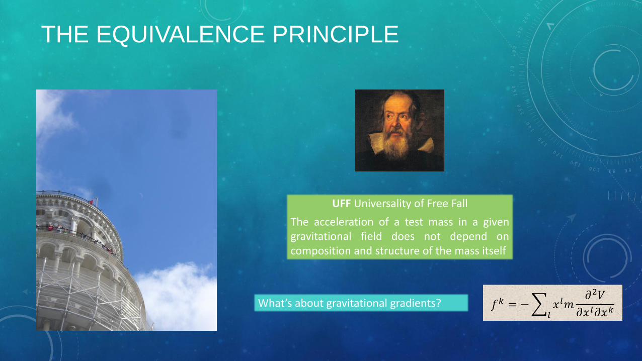
THE EQUIVALENCE PRINCIPLE

UFF Universality of Free Fall

The acceleration of a test mass in a given gravitational field does not depend on composition and structure of the mass itself

What’s about gravitational gradients? 𝑓𝑘 = − 𝑥𝑙𝑚𝜕2𝑉

𝜕𝑥𝑙𝜕𝑥𝑘𝑙

THE EQUIVALENCE PRINCIPLE

Will 2014 Dicke 1964 Ciufolini – Wheeler 1995 Turyshev 2008

WEP WEP EP (weak form)

+LLI +LPI

EP (medium strong form) WEP

SEP EP (very strong form) SEP

EEP SEP

+UFF +LLI EP +LPI

EP: SOME DEFINITIONS...

EEP Einstein Equivalence Principle

• WEP Weak Equivalence Principle • LLI Local Lorentz Invariance • LPI Local Position Invariance

Test masses

Non-gravitational experiments

Metric theories

• Spacetime with a symmetric metrics • Trajectories of test masses: geodetics • In a locally freely-falling frame, the laws of physics are those of

Special Relativity

EP: SOME DEFINITIONS...

SEP Strong Equivalence Principle

• WEP Weak Equivalence Principle • LLI Local Lorentz Invariance • LPI Local Position Invariance

Also self-gravitating masses

Gravitational and non-gravitational experiments

Practically only General Relativity (among the known and «reasonable» theories) satisfies the SEP

WEP TESTS

Will 2014

Future (proposed) missions GReAT 5 x 10-15

MICROSCOPE 10-15 POEM 10-16 I.C.E. 10-16 GG 10-17 STEP 10-18

WEP TESTS

Courtesy Anna Maria Nobili

WEP TESTS

WEP TESTS

Eot-Wash

• Sun or Earth as sources of the gravitational field

• Signal modulation • Control of gravitational (multipoles)

and non-gravitational systematics

SEP

𝐸

𝑚𝑐2 𝑖= −

𝐺

2𝑚𝑖𝑐2

𝜌𝑖(𝑟)𝜌𝑖(𝑟′)

𝑟 − 𝑟′𝑑3𝑥𝑑3𝑥′

𝑖

Gravitational contribution to the system energy

System E/mc2

Sun 10-6

Earth 10-10

Moon 10-11

Laboratory body 10-25

𝑚p

𝑚i= 1 − 𝜂N

𝐸

𝑚𝑐2

𝜂N = 4𝛽 − 𝛾 − 3 −10

3𝜉 − 𝛼1 +

2

3𝛼2 −

2

3𝜎1 −

1

3𝜎2

Nordtvedt effect 𝛿𝑟 = 13.1𝜂N cos 𝜔0 − 𝜔s 𝑡 LLR

Anderson+ 1996, Merkowitz 2010

INVERSE-SQUARE LAW

Why should it be necessarily 𝐹 ∝1

𝑟2 ?

Fischbach+ 1986: Proposal of a Fifth Force Such an intermediate-range force – together with gravitation – would cause a net interaction among macroscopic bodies, with consequent (small) deviations from inverse-square law

Recurrent theoretical motivations: • Wagoner 1970, Fuji 1971, O’ Hanlon 1972 • Damour+Nordtvedt 1993, Damour+Polyakov 1994,

Damour+ 2002, Veneziano 2002, …

𝑉5 𝑟 = −𝛼𝐺𝑚𝑖𝑚𝑗

𝑟𝑒−𝑟𝜆 𝑚Γ =

ℏ

𝜆𝑐

𝛼 > 0: attractive force

𝑉 𝑟 = 𝑉𝑁 𝑟 + 𝑉5 𝑟 = −𝐺𝑚𝑖𝑚𝑗

𝑟1 + 𝛼𝑒

−𝑟𝜆

𝐹 𝑟 = −𝛻𝑉 𝑟 = −𝐺(𝑟)𝑚𝑖𝑚𝑗

𝑟𝑟

𝐺 𝑟 = 𝐺∞ 1 + 𝛼 1 +𝑟

𝜆𝑒−𝑟𝜆

Exchange of spin-1 quanta → Repulsive → Composition-dependent effects Exchange of spin-0 or spin-2 quanta → Attractive → Composition-independent effects

INVERSE-SQUARE LAW

𝛼𝑖𝑗 = −𝜉𝐵𝑖𝜇𝑖

𝐵𝑗

𝜇𝑗 𝜇𝑖,𝑗 =

𝑚𝑖,𝑗

𝑚𝐻

Possible interaction dependent on ipercharge Y = B +S For macroscopic bodies it is considered Y = B

Deviation from 1/r, G(r) ≠ const → Composition independent αij ≠ const → Composition dependent

Composition independent • Measurement of g(z) on towers (Laplace

equation) • Measurement of g as a function of water height

in a basin • Airy method applied to oceans • Test mass inside a cylinder • Laplacian measurement • G measurement (LAGEOS, Moon, planets) • Pericenter advance (LAGEOS II, planets)

Composition dependent • Torsion balance • Fluctuating balls • Resonant detector for gravitational waves • Free fall

INVERSE-SQUARE LAW

Adelberger+ 2003

INVERSE-SQUARE LAW

Adelberger+ 2003

MEASUREMENT OF G

Schlamminger 2014

KERR METRIC

dtdrc

GJddrdr

rc

GMdtc

rc

GMds 2

2

22222

1

2

22

2

2 sin4

sin2

12

1

Kerr metric in weak field (it describes in an approximate way the spacetime around a rotating mass)

g

!!! Mach?

BARICENTRIC EQUATIONS OF MOTION

Moyer 2000

GEOCENTRIC EQUATIONS OF MOTION

IERS Conventions (2010)

Effect Ratio to monopole

Schwarzschild 10-9 – 10-10

Lense-Thirring 10-11 – 10-12

De Sitter 10-11 – 10-12

• Ashby+Bertotti 1984, 1986 • Brumberg+Kopeikin 1989 • Huang+ 1990 • Brumberg 1991 • Damour+ 1991, 1992, 1993, 1994 • … • Soffel+ 2003

Relativistic corrections:

GRAVITOMAGNETISM

TRgR 82

1

hg

ii vh 160

2

Weak field

Lorentz gauge

hH

ih0 Gravitomagnetic potential

Gravitomagnetic field

Defined by analogy with the electromagnetic case

Moving (rotating) masses: what do they do? — Spacetime

GRAVITOMAGNETISM Moving (rotating) masses: what do they do? — Geodesics

02

2

2

d

xd

d

dx

d

xd

Slow-motion

H

dt

xdGm

dt

xdm

2

2

Gravitoelectric field

Gravitomagnetic contribution

Thus mass-energy currents influence the motion of test

masses: Gravitomagnetism

PERTURBATION ANALYSIS

Lagrange perturbation equations Gauss perturbation equations

a

R

nae

R

ena

en

dt

dM

e

R

ena

e

I

R

ena

I

dt

d

I

R

Ienadt

d

R

Iena

R

ena

I

dt

dI

R

ena

e

M

R

ena

e

dt

de

M

R

nadt

da

21

1

1

cot

sin1

1

sin1

1

1

cot

11

2

2

2

2

2/12

2/122

2/122

2/1222/122

2

2/12

2

2

t

tdtnM

dI

dt

deR

a

r

nadt

d

fIrH

W

e

ufTfR

nae

e

dt

d

frIH

W

dt

d

frH

W

dt

dI

ufTfRna

e

dt

de

feTfendt

da

0

2/12

2/12

2/12

2/12

2/12

dtcos1

2

sincot1

sinsincos

1

sinsin

cos

coscossin1

cos1sinRe1

2

PERTURBATION ANALYSIS Einstein or Schwarzschild precession

Using Lagrange equations

eena

e

anan

dt

dM

Iena

I

eena

e

dt

d

IIenadt

d

IIenadt

dI

Me

ena

e

dt

de

Mnadt

da

n

2

2

222

2

22

22

2

2

2

12

1

cot1

sin1

1

cossin1

1

11

2

q

q qMeGa

e

c

GMR cos

1212

22

q

q

q

q

q

q

q

q

q

q

qMeGqMeGe

e

a

e

c

GMn

dt

dM

qMeGea

e

c

GM

dt

d

dt

d

dt

dI

qMeqGea

e

c

GM

dt

de

qMeqGa

e

c

GM

dt

da

cos6cos'11

cos'1

0

0

sin1

sin12

2121

2

25

2

2

23

2125

232

2

23

2125

22

2

23

2123

2

2

23

The orbital plane remains fixed in space

Only short period effects

q = 0

0

0

sec

sec

dt

de

dt

da

Secular effects

Perturbing function

PERTURBATION ANALYSIS

dt

dI

dt

defe

pna

IGJ

dt

d

dt

dIfef

e

e

ap

IGJ

dt

d

feffeffefp

GJ

dt

d

feffeffefp

IGJ

dt

dI

fefap

IGJ

dt

de

dt

da

cos1cos1cos4

coscos1cos1

2cos

cos1)sin(cos12)cos(sinsin

cos1)sin(cos12)cos(sincossin

cos1sincos

0

23

32

'

22

2

2

3

2

3

2

2

No effects in the semimajor axis

In order to obtain the secular and long period effects the average of the mean anomaly M is calculated

)(2sinsinsin

)(2coscoscos

2

2

eMeMf

eMeeMf

2

02 2

1dM

dt

d

dt

d Long period

Secular

Lense–Thirring precession

𝜔

Ω

TEST MASS

General relativity (geometrodynamics) implies a continuous feedback between geometry and mass-energy (nonlinearity)

Practical needs often force to “hold on something”

TEST MASS • No electric charge • Gravitational bounding energy negligible with

respect to rest mass-energy • Angular momentum negligible • Sufficiently small to neglect tidal effects

TEST MASS

The Moon The smallness of a test mass depends

on the scale under consideration

LAGEOS satellites Probably the closest to the ideal concept of a test mass

TEST MASS

Cassini A test mass in the outer solar system

BepiColombo A future test mass pretty close to the Sun

TRACKING – SATELLITE LASER RANGING

Retroreflectors mounted on the satellite surface are the target for laser pulses, whose round-trip light time is precisely measured. ILRS stations directly contribute to ITRF.

• Very simple in principle, but requires ILRS dedicated tracking • Coverage depends on stations schedule and atmospheric conditions • Observable: range, 1 mm precision • POD: sub-dm, approaching the cm level depending on model choices

Photo by Franco Ambrico; courtesy Giuseppe Bianco, ASI-CGS

2

tcs

ilrs.gsfc.nasa.gov

TRACKING – SATELLITE LASER RANGING

ilrs.gsfc.nasa.gov

TRACKING – RADIOMETRIC

Microwave signals are exchanged between ground stations and an on-board transponder. By very precise frequency standards, range and range-rate can be derived.

• Very complex system (both ground and space segment) • 24 hr coverage (DSN) • Observables: range, sub-m precision; range-rate, 10-5 ms-1 precision

• POD: sub-m (depends on model choices)

JPL

𝑓R = 1 −𝜌

𝑐𝑓T

Doppler shift

In practice, the total phase change is measured. The Doppler count provides a measure of range change during integration time Tc.

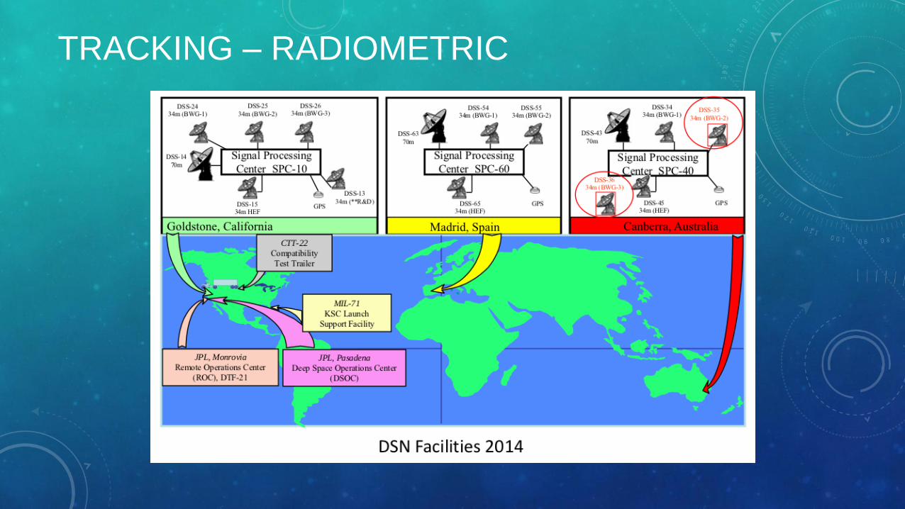
TRACKING – RADIOMETRIC

Microwave signals are exchanged between ground stations and an on-board transponder. By very precise frequency standards, range and range-rate can be derived.

• Very complex system (both ground and space segment) • 24 hr coverage (DSN) • Observables: range, sub-m precision; range-rate, 10-5 ms-1 precision

• POD: sub-m (depends on model choices)

JPL

𝑓R = 1 −𝜌

𝑐𝑓T

Doppler shift

In practice, the total phase change is measured. The Doppler count provides a measure of range change during integration time Tc.

Tornton+Border 2000

TRACKING – RADIOMETRIC

PRECISE ORBIT DETERMINATION

Differential correction procedure

W

P

CM

COf

dPz

j

iij

iii

ii

j ij

j

iii dOdP

P

CCO

fWMMWMz TT 111

Corrections to the models parameters

Residuals

Observation equations

Least-squares (normal equations)

Partials

Covariance matrix

LAGEOS SATELLITES

LAGEOS LAGEOS II

– COSPAR ID 7603901 9207002

– Launch date 4 May 1976 22 October 1992

– Diameter 60 cm 60 cm

M Mass 406.965 kg 405.38 kg

– Retroreflectors 426 CCR 426 CCR

a Semimajor axis 1.2286 · 107 m 1.2155 · 107 m

e Eccentricity 0.0045 0.0135

I Inclination 109.84° 52.64°

– Perigee height 5.86 · 106 m 5.62 · 106 m

P Period 225 min 223 min

n Mean motion 4.654 · 10−4 s−1 4.696 · 10−4 s−1

Node rate 0.34266° d−1 -0.62576641° d−1

Perigee rate -0.21338° d−1 0.44470485° d−1

INFN CSN2 Roma2 Team led by David

M. Lucchesi

Numerical values for the secular relativistic precessions on the argument of pericenter and node of the two LAGEOS satellites:

Total values for LAGEOS II

Total values for LAGEOS

1 mas = 1 milli arc sec

mas/yr 95.3294L2

rel

mas/yr 77.3310L1

rel

RELATIVISTIC PRECESSIONS

Rate (mas/yr) LAGEOS II LAGEOS

+ 3351.95 + 3278.77

– 57.00 + 32.00

+ 31.48 + 30.65

+ 17.60 + 17.60

E

LT

LT

dS

MODELS

The analysis of experimental data to obtain the properties of a physical system requires models

• System dynamics • Measurement procedure • (Reference frame)

The availability of good experimental data implies taking out a lot of “noise” in order to reach the phenomenology of interest – many orders of magnitude, in case of relativistic effects

MODELS

• Geopotential (static part) • Solid Earth and ocean tides / Other temporal variations of

geopotential • Third body (Sun, Moon and planets) • de Sitter precession • Deviations from geodetic motion • Other relativistic effects • Direct solar radiation pressure • Earth albedo radiation pressure • Anisotropic emission of thermal radiation due to visible

solar radiation (Yarkovsky-Schach effect) • Anisotropic emission of thermal radiation due to infrared

Earth radiation (Yarkovsky-Rubincam effect) • Asymmetric reflectivity • Neutral and charged particle drag

Gravitational

Non-gravitational

MODELS

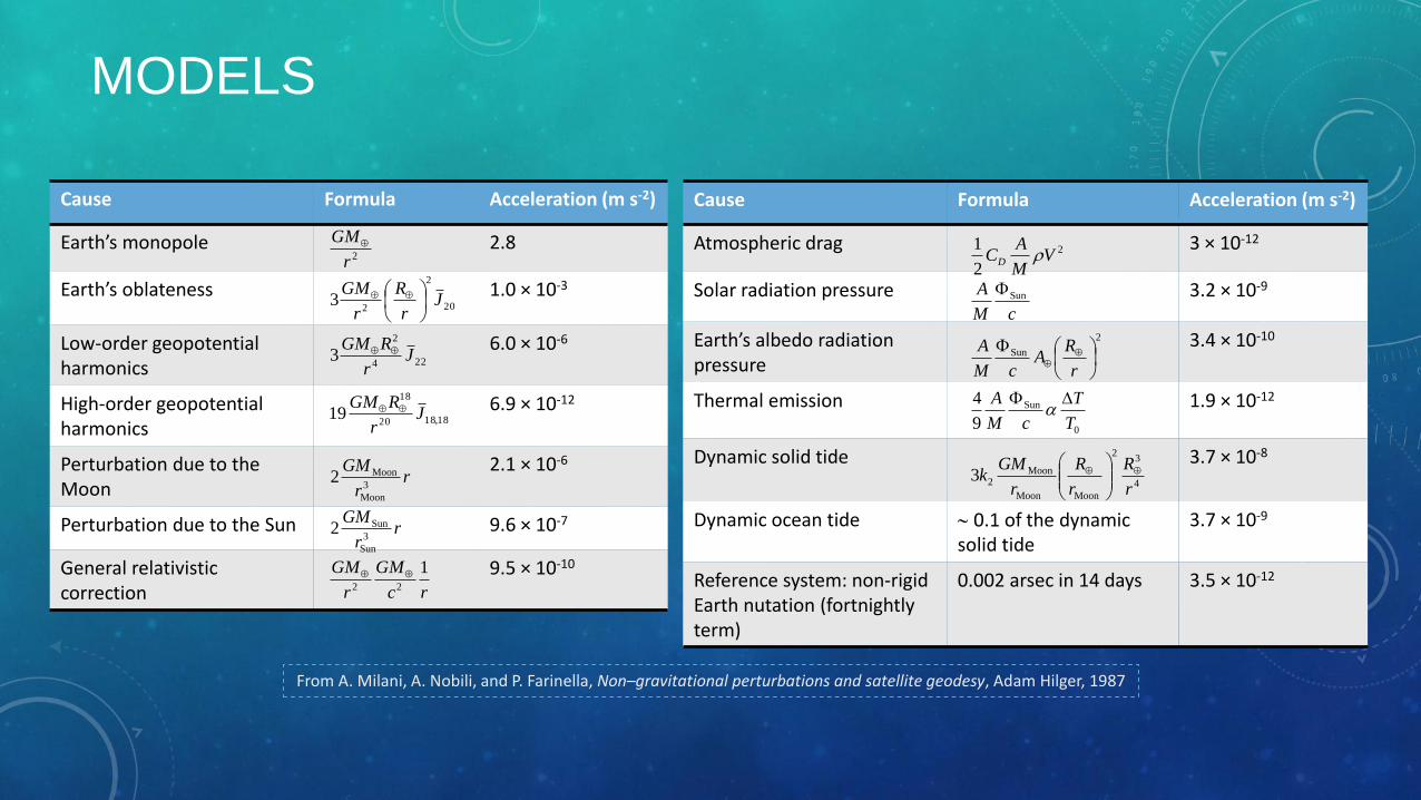
Cause Formula Acceleration (m s-2)

Earth’s monopole 2.8

Earth’s oblateness 1.0 × 10-3

Low-order geopotential harmonics

6.0 × 10-6

High-order geopotential harmonics

6.9 × 10-12

Perturbation due to the Moon

2.1 × 10-6

Perturbation due to the Sun 9.6 × 10-7

General relativistic correction

9.5 × 10-10

From A. Milani, A. Nobili, and P. Farinella, Non–gravitational perturbations and satellite geodesy, Adam Hilger, 1987

2r

GM

20

2

23 J

r

R

r

GM

224

2

3 Jr

RGM

18,1820

18

19 Jr

RGM

rr

GM3

Moon

Moon2

rr

GM3

Sun

Sun2

rc

GM

r

GM 122

Cause Formula Acceleration (m s-2)

Atmospheric drag 3 × 10-12

Solar radiation pressure 3.2 × 10-9

Earth’s albedo radiation pressure

3.4 × 10-10

Thermal emission 1.9 × 10-12

Dynamic solid tide 3.7 × 10-8

Dynamic ocean tide 0.1 of the dynamic solid tide

3.7 × 10-9

Reference system: non-rigid Earth nutation (fortnightly term)

0.002 arsec in 14 days 3.5 × 10-12

2

2

1V

M

ACD

cM

A Sun

2

Sun

r

RA

cM

A

0

Sun

9

4

T

T

cM

A

4

32

MoonMoon

Moon23

r

R

r

R

r

GMk

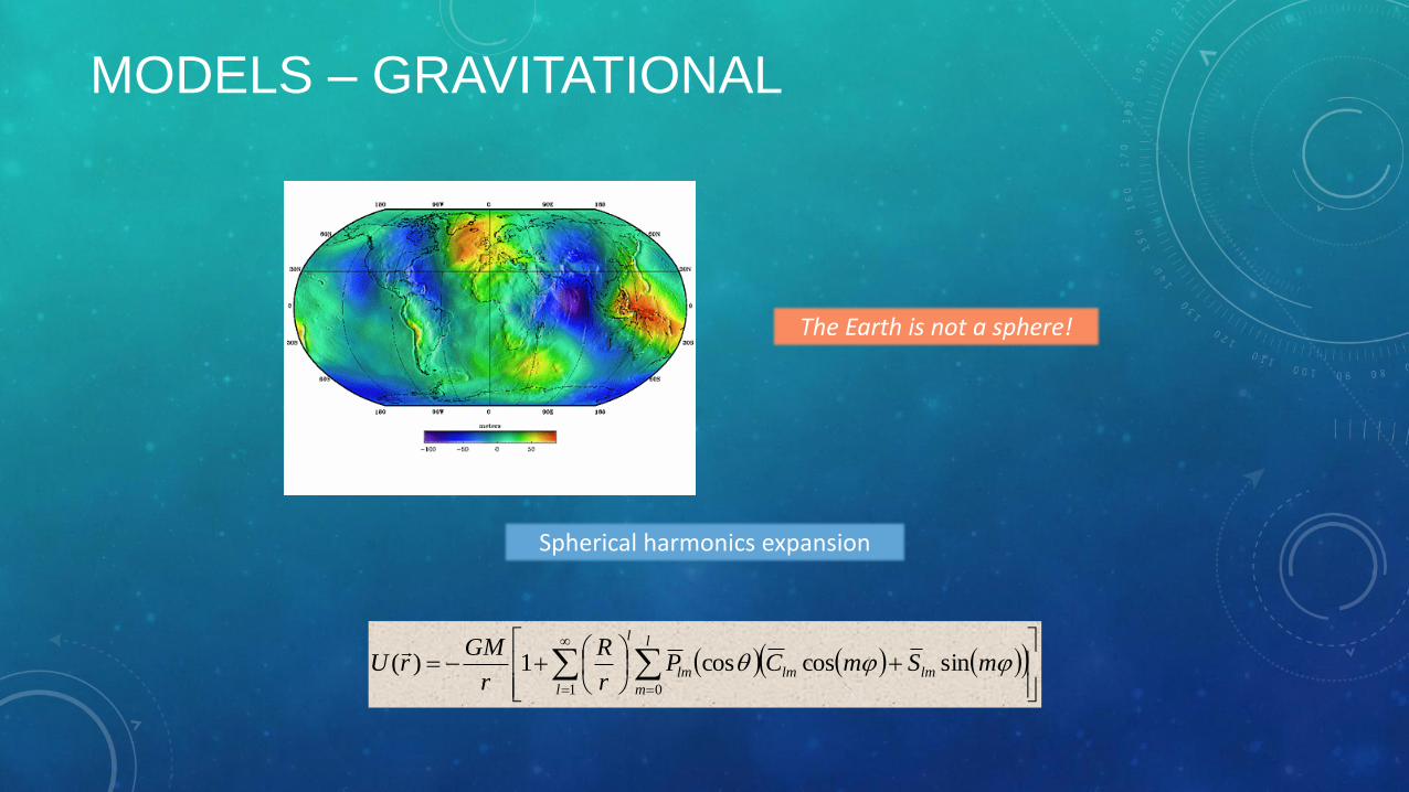
MODELS – GRAVITATIONAL

The Earth is not a sphere!

Spherical harmonics expansion

1 0

sincoscos1)(l

l

m

lmlmlm

l

mSmCPr

R

r

GMrU

MODELS – GRAVITATIONAL

The Earth is not a sphere!

Spherical harmonics classification

Zonal

Tesseral

Sectorial

0m

0m

lm

lm

0m

MODELS – GRAVITATIONAL

Quadrupole perturbation (l = 2, m = 0) to first order

2/32

22

20

22

22

20

22

2

20

1

cos31

4

3

1

cos51

4

3

1

cos

2

3

0

0

0

e

I

a

RnCn

dt

dM

e

I

a

RnC

dt

d

e

I

a

RnC

dt

d

dt

dI

dt

de

dt

da

Some geopotential models

Model Data type Maximum degree

JGM-3 Combined 70

GRIM5-S1 Satellite 95

GRIM5-C1 Combined 120

OSU89A/B Combined 360

EGM96 Combined 360

EIGEN-2 Satellite 120

EIGEN-GRACE02S Satellite 150

GGM02S Satellite 160

MODELS – GRAVITATIONAL

Geoid (EIGEN-GRACE02S) The geoid is a gravitational equipotential surface, taken as reference surface (“sea level”); it differs

in general from a rotation surface, like the reference ellipsoid

MODELS – GRAVITATIONAL

Gravity anomalies (EIGEN-GRACE02S) The gravity anomalies are the difference between the real gravity field and that of a reference body

(rotation ellipsoid)

MODELS – GEOPOTENTIAL

The degree variance is useful when comparing various geopotential solutions

Its behaviour is well described by the so-called Kaula’s rule

l

m

lmlml SCl

C0

222

12

1

4

102 10

7.0l

Cl

MODELS – GEOPOTENTIAL

The degree variance is useful when comparing various geopotential solutions

Its behaviour is well described by the so-called Kaula’s rule

l

m

lmlml SCl

C0

222

12

1

4

102 10

7.0l

Cl

MODELS – NON GRAVITATIONAL

It is due to reflection-diffusion-absorption of solar photons from the spacecraft surface

• The strongest among the non-gravitational perturbations

• Well modeled for LAGEOS (though the CR estimate could be biased due to some other not modeled signal)

Direct solar radiation pressure

www.pmodwrc.ch/pmod.php?topic=tsi/composite/SolarConstant

sr

AU

mc

ACa ˆ

12

R

MODELS – NON GRAVITATIONAL Solar Yarkovsky-Schach effect

It is due to infrared radiation anisotropically emitted from the satellite (warmed by the Sun)

• Effective on argument of perigee behaviour • Difficult modelization (the acceleration depends on S)

𝑎 𝑧 =16

9𝜋𝑅2

휀𝜍

𝑚𝑐𝑇03∆𝑇 cos 𝜗𝑠Γ𝑧(𝜆)𝑧

𝑎 𝑥 =16

9𝜋𝑅2

휀𝜍

𝑚𝑐𝑇03∆𝑇 sin𝜗𝑠

Γ𝑥(𝜆, 𝑁)

1 + 𝑁2𝜍𝑅2 𝑥

𝑎 𝑦 =16

9𝜋𝑅2

휀𝜍

𝑚𝑐𝑇03∆𝑇 sin𝜗𝑠

Γ𝑦(𝜆, 𝑁)

1 + 𝑁2𝜍𝑅2 𝑦

Rapid spin approximation: the disturbing acceleration has only a component along the rotation axis

General spin approximation: the disturbing acceleration has in addition also two equatorial components

MODELS – SPIN

LAGEOS LAGEOS II

MODELS - REFERENCE FRAMES

ICRF

Precession

Nutation

Length of Day

Pole motion

ITRF

DATA ANALYSIS

Feature Model

Geopotential (static part) EGM96, EIGEN-2, GGM01S, EIGEN-GRACE02S

Geopotential (tides) Ray GOT99.2

Third body JPL DE-403

Relativistic corrections PPN

Direct solar radiation pressure Cannonball

Albedo radiation pressure Knocke–Rubincam

Earth-Yarkovsky Rubincam 1987-1990

Spin axis evolution Farinella et al. 1996

Stations positions (ITRF) ITRF2000

Ocean load Scherneck with GOT99.2 tides

Pole motion IERS EOP

Earth rotation IERS EOP

IERS Conventions (2010)

POD

Reference orbit Orbit used in the analysis

POD

LENSE-THIRRING

IIII

2

I

2I

TL

IIII

2

I

2TL

I

N

N

N

N

The recent geopotential models make critical in the error budget only the uncertainty associated with C20 (Earth quadrupole)

Two-node combination to overcome this problem

RP, Ciufolini+ 2006

LENSE-THIRRING

IIII

2

I

2I

TL

IIII

2

I

2TL

I

N

N

N

N

The recent geopotential models make critical in the error budget only the uncertainty associated with C20 (Earth quadrupole)

Two-node combination to overcome this problem

RP, Ciufolini+ 2006

RP

The perturbation due to the YARKOVSKY–SCHACH effect is clear from the residuals

Pericenter rate (mas/yr) Integrated Pericenter (mas)

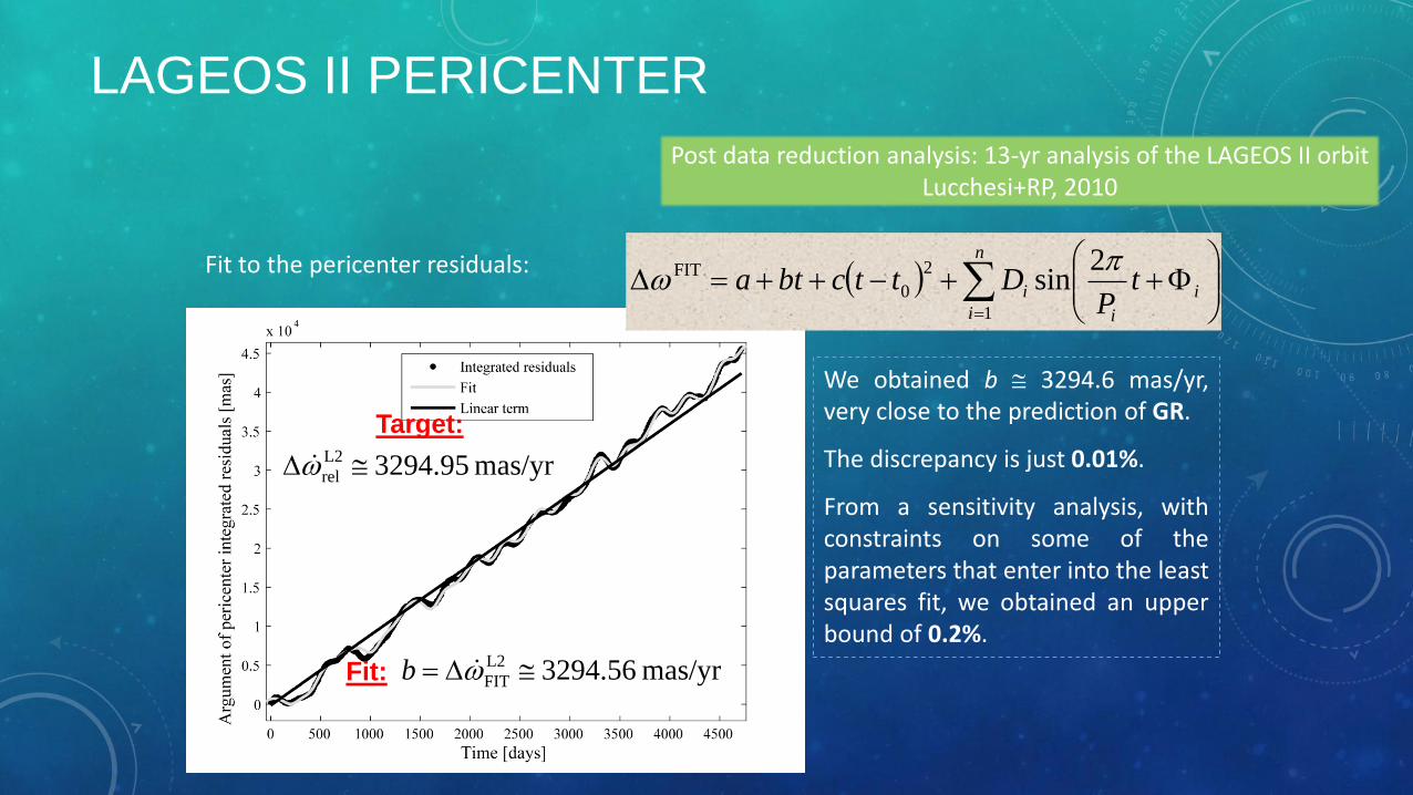
Post data reduction analysis: 13-yr analysis of the LAGEOS II orbit Lucchesi+RP, 2010

LAGEOS II PERICENTER

LAGEOS II PERICENTER

Target:

Fit:

We obtained b 3294.6 mas/yr, very close to the prediction of GR.

The discrepancy is just 0.01%.

From a sensitivity analysis, with constraints on some of the parameters that enter into the least squares fit, we obtained an upper bound of 0.2%.

Fit to the pericenter residuals:

mas/yr 56.3294L2

FIT b

mas/yr 95.3294L2

rel

i

i

n

i

i tP

Dttcbta

2

sin1

2

0

FIT

Post data reduction analysis: 13-yr analysis of the LAGEOS II orbit Lucchesi+RP, 2010

Error budget (systematic effects estimate) for LAGEOS II pericenter

Lucchesi+RP, 2014

LAGEOS II PERICENTER 휀 = 1 + (−0.12 ± 2.10) ∙ 10−3 ± 2.5 ∙ 10−2

CONSTRAINTS ON GRAVITATION THEORIES

Constraints on the post-Newtonian parameters

휀 = 1 + (−0.12 ± 2.10) ∙ 10−3 ± 2.5 ∙ 10−2

The parameter may be considered at the PN level and, because the bulk of the effect is due to Einstein’s precession of the pericenter, we can assume:

Shapiro+ 1989, radar ranging to Mercury (perihelion shift)

Williams+ 2001, Lunar Laser Ranging (equation of motion)

2 + 2𝛾 − 𝛽

3− 1 ≅ 1 ∙ 10−3 ± 2 ∙ 10−2

𝛽 + 𝛾 − 2 ≅ 7 ∙ 10−4 ± 1.4 ∙ 10−3

2 + 2γ − β

3− 1 ≅ ε − 1 = −(0.12 ± 2.10) ∙ 10−3 ± 2.5 ∙ 10−2

Δ𝜔 = Δ𝜔 GP + Δ𝜔 NGP + 휀Δ𝜔 GR

Therefore, with the present study we can constrain the strength of a Yukawa-like interaction, to the following value:

Which represents an improvement of several orders-of-magnitude with respect to previous results based on Earth-LAGEOS and LAGEOS-Lunar measurements

Lucchesi+RP, 2010

Constraints on a long-range force: Yukawa-like interaction

CONSTRAINTS ON GRAVITATION THEORIES

R1km 6081[mas/yr] 102923586.8 11 Yuk

1212 10691085.0

Lucchesi+RP, 2014

CONSTRAINTS ON GRAVITATION THEORIES

Adelberger+ 2003

CONSTRAINTS ON GRAVITATION THEORIES

Δ𝜔 𝑠𝑒𝑐𝑀𝑜𝑓𝑓𝑎𝑡

=3 𝐺𝑀⊕

3 2

𝑐2𝑎5 2 1 − 𝑒2𝒞⊕𝒮

𝑐4 1 + 𝑒2 4

𝐺𝑀⊕ 1 − 𝑒22

𝒞⊕𝐿𝑎𝑔𝑒𝑜𝑠𝐼𝐼 ≤ 0.003𝑘𝑚 4 ± 0.036𝑘𝑚 4 ± 0.092𝑘𝑚 4

Moffat non-symmetric theory

Ciufolini+Matzner 1992, from the total uncertainty in the calculated precession of LAGEOS

Lucchesi 2003, from the systematic effects on the pericenter of LAGEOS II

𝒞⊕𝐿𝑎𝑔𝑒𝑜𝑠 ≤ 0.16𝑘𝑚 4

𝒞⊕𝐿𝑎𝑔𝑒𝑜𝑠𝐼𝐼 ≤ 0.087𝑘𝑚 4

Δ𝜔 𝑠𝑒𝑐𝑡𝑜𝑟𝑠𝑖𝑜𝑛 =

3 𝐺𝑀⊕3 2

𝑐2𝑎5 2 1−𝑒22𝑡2+𝑡3

3+∆𝜔 𝐿𝑇

𝑡𝑜𝑟𝑠𝑖𝑜𝑛 Mao spacetime torsion

2𝑡2 + 𝑡3 ≤ 3.5 ∙ 10−4 ± 6.2 ∙ 10−3 ± 7.49 ∙ 10−2

March+ 2011, using the Mercury's perihelion shift measurement of Shapiro+ 1990 2𝑡2 + 𝑡3 ≅ 3 ∙ 10−3

GPS

Ashby 2003

Δ𝑡 = 1 +3𝐺𝑀⨁

2𝑎𝑐2+𝑉0𝑐2

−2𝐺𝑀⨁

𝑐21

𝑎−1

𝑟𝑑𝜏

path

Elapsed coordinate time on spacecraft clock:

-4.4647 × 10-10

- Gravitational blueshift + Second-order Doppler shift

Eccentricity correction

LUNAR LASER RANGING

Three retroreflectors arrays were carried on The Moon by Apollo missions and two by Soviet missions

Probably the most important scientific contribution from Apollo missions!

Selenodesy Lunar rotation General relativity

LUNAR LASER RANGING

Three retroreflectors arrays were carried on The Moon by Apollo missions and two by Soviet missions

Probably the most important scientific contribution from Apollo missions!

Selenodesy Lunar rotation General relativity

LUNAR LASER RANGING

Nordtvedt 1996

LUNAR LASER RANGING

Nordtvedt 1996

Type Measurement Reference

EP Δ

𝑀G

𝑀I SEP

= −2.0 ± 2.0 × 10−13 Baeßler+ 1999 Williams + 2004 Schlamminger+ 2008 𝜂 = 4.4 ± 4.5 × 10−4

𝐺 𝐺

𝐺= 6 ± 7 × 10−13 yr−1 Turyshev+Williams 2007

𝐺

𝐺= 2 ± 7 × 10−13 yr−1

Müller+Biskupek 2007 𝐺

𝐺= 4 ± 5 × 10−15 yr−2

Yukawa 𝛼 < 5.9 × 10−11 @ 𝜆 = 𝑎/2 Merkowitz 2010

𝛼 = 3 ± 2 × 10−11 @ 𝜆 = 4 × 105 km Müller+ 2008

de Sitter 𝐾dS = 1.9 ± 6.4 × 10−3 Williams + 2004

PPN 𝛽 − 1 = 1.2 ± 1.1 × 10−4 Williams + 2004 (+ CASSINI)

𝛼1 = −7 ± 9 × 10−5 Müller+ 2008

𝛼2 = 1.8 ± 2.5 × 10−5

CASSINI

Bertotti+ 2003

𝛾 = 1 + 2.1 ± 2.3 × 10−5

Δ𝑡 = 2 1 + 𝛾𝐺𝑀⨀

𝑐3ln

4𝑟1𝑟2𝑏2

Δ𝜈

𝜈=𝑑Δ𝑡

𝑑𝑡= −2 1 + 𝛾

𝐺𝑀⨀

𝑐3𝑏

𝑑𝑏

𝑑𝑡 Frequency shift of photons:

Round trip time:

CASSINI

Bertotti+ 2003

𝛾 = 1 + 2.1 ± 2.3 × 10−5

Δ𝑡 = 2 1 + 𝛾𝐺𝑀⨀

𝑐3ln

4𝑟1𝑟2𝑏2

Δ𝜈

𝜈=𝑑Δ𝑡

𝑑𝑡= −2 1 + 𝛾

𝐺𝑀⨀

𝑐3𝑏

𝑑𝑏

𝑑𝑡 Frequency shift of photons:

Round trip time:

Turyshev 2008

OPTICAL SPACETIME CURVATURE TEST

FROM NY ALESUND

• Optical experiments were done (1919 Eddington to 1973 Univ. Texas) to test light deflection close to the Sun (using photographic plates), marginal results

• A new optical test is planned for the March 2015 total solar eclipse from Ny Alesund, Svalbard

• Strategy is to use 2 telescopes (10.8 and 12.5 cm refractors on same mount) CCD/CMOS cameras

• Solar region annulus 2R -3R, FOV, (12.5 cm) X: 39' 34“ Y: 29' 47“ (10.8 cm) X: 10' 18“ Y: 7' 38“

• Expected accuracy in the isokinetic region ~ 200 milli-arcsec

Info courtesy Ludwig Combrinck

BEPICOLOMBO

The Radio Science Experiments (RSE) use the BepiColombo radiometric tracking measurements from ground antennas to precisely locate (position and velocity) the spacecraft and obtain informations on the gravitational dynamics environment

• Gravimetry • Rotation • General relativity

Three main experiments: Involved instruments:

• Ka band Transponder • Star–Tracker • High-resolution camera • Accelerometer

BEPICOLOMBO

• The global gravity field of Mercury and its temporal variations due to solar tides (in order to constrain the internal structure of the planet)

• The local gravity anomalies (in order to constrain the mantle structure of the planet and the interface between mantle and crust)

• The rotation state of Mercury (in order to constrain the size and the physical state of the core of the planet) • The orbit of Mercury center of mass around the Sun (in order to improve the determination of the

parameterized post–Newtonian (PPN) parameters of general relativity)

Milani+ 2001, 2002

• Range and range–rate tracking of the MPO with respect to Earth–bound radar station(s) (and then of Mercury center of mass around the Sun)

• Determination of the non–gravitational forces acting on the MPO by means of an on–board accelerometer • Determination of the MPO absolute attitude by means of a Star–Tracker • Determination of angular displacements of reference points on the solid surface of the planet, by means of a

camera

BEPICOLOMBO

• Spherical harmonic coefficients of the gravity field of the planet up to degree and order 25 • Degree 2 (C20 and C22) with 10-9 accuracy (Signal/Noise Ratio 104) • Degree 10 with SNR 300 • Degree 20 with SNR 10 • Love number k2 with SNR 50 • Obliquity of the planet to an accuracy of 4 arcsec (40 m on surface – needs also SYMBIO-SYS) • Amplitude of physical librations in longitude to 4 arcsec (40 m on surface – needs SYMBIO-SYS) • Cm/C (ratio between mantle and planet moment of inertia) to 0.05 or better • C/MR2 to 0.003 or better

• Spacecraft position in a Mercury-centric frame to 10 cm – 1m (depending on the tracking geometry) • Planetary figure, including mean radius, polar radius and equatorial radius to 1 part in 107 • Geoid surface to 10 cm over spatial scales of 300 km • Position of Mercury in a solar system baricentric frame to better than 10 cm

• to 2.5∙10-6

• to 5∙10-6

• η to 2∙10-5

• Gravitational oblateness of the Sun (J2) to 2∙10-9

• Time variation of the gravitational constant (d(lnG)/dt) to 3∙10-13 years-1 Milani+ 2001, 2002

ITALIAN SPRING ACCELEROMETER

ISA oscillator parameters:

Mass 200 g

Resonance frequency 3.9 Hz

Mechanical quality factor 10

ISA performance:

Measurement bandwidth 3 x 105 – 1x 101 Hz

Intrinsic noise 1 x 109 m/s2/Hz

Measurement accuracy 1 x 108 m/s2

Dynamics 300 x 108 m/s2

A/D converter saturation 3000 x 108 m/s2

ISA thermal stability:

Sensor thermal sensitivity 5 x107 m/s2/°C

Electronic thermal sensitivity 1 x108 m/s2/°C

Active thermal control attenuation 700

Temperature variations:

Mercury half sidereal period (44 days) 25°C peak-to-peak

MPO orbital period (2.325 h) 4°C peak-to-peak

Random noise 10°C /Hz

ITALIAN SPRING ACCELEROMETER

ANOMALIES...

Anderson+ 2002 Turyshev+ 2012

𝑎P = 8.74 ± 1.33 × 10−10 m/s2

BIASES...

RP Lucchesi+ 2004

Probably a false signal A true signal?

UNEXPECTED RESULTS...

Geopotential harmonics coefficients change in time: • Tides • Secular variations (e.g. postglacial rebound) • Mass transport (e.g. oceans ↔ atmosphere)

This variation seems to be due to an abrupt change in the quadrupole rate (Cox+Chao, 2002; Ciufolini+, 2006) The causes are uncertain: • Mantle? • Tides? In any case, this implies a net mass transfer from polar to equatorial regions

CURRENT STATUS

Turyshev 2008

READINGS (MINIMAL SET)

Books • H. C. Ohanian and R. Ruffini, Gravitation and space-time, Cambridge University Press, 20133

• I. Ciufolini and J. A. Wheeler, Gravitation and Inertia, Princeton University Press, 1995 • C. Will and E. Poisson, Gravity: Newtonian, Post-Newtonian, Relativistic, Cambridge University Press, 2014 • B. Bertotti, P. Farinella and D. Vokrouhlický, Physics of the Solar System — Dynamics and Evolution, Space

Physics, and Spacetime Structure, Kluwer Academic Publishers, 2003 • O. Montenbruck and E. Gill, Satellite Orbits — Models, Methods and Applications, Springer, 2000

Reviews • C. M. Will, The Confrontation between General Relativity and Experiment, Living Rev. Relativity 17, (2014), 4,

http://www.livingreviews.org/lrr-2014-4 • N. Ashby, Relativity in the Global Positioning System, Living Rev. Relativity 6, (2003), 1,

http://www.livingreviews.org/lrr-2003-1 • S. M. Merkowitz, Tests of Gravity Using Lunar Laser Ranging, Living Rev. Relativity 13, (2010), 7,

http://relativity.livingreviews.org/Articles/lrr-2010-7/ • E. Fischbach and C. Talmadge, Six years of the fifth force, Nature 356, 207 (1992)