SOLAR FLARES AND CMES OBSERVED IN LINEAR AND CIRCULAR POLARISATION WITH

THE CALLISTO AND OTHER INSTRUMENTS

ROOPA Nandita PIRTHEE SagarGirish Kumar Beeharry

IEEE AFRICON URSI BEJ Conference(Mauritius September 2013)

2

AIMS ● Monitoring Solar Flares and CMEs in both linear & circular polarisation

with the CALLISTO (Range: 45 to 870 MHz)

● Classifying the FITS files containing solar flares into different flare types.

● Conducting background subtraction, addition and comparison of data

using Python scripts in SunPy.

● Analysing CALLISTO data in conjunction with Nobeyama, Nançay and LASCO data.

● Observation of the 2 hour long (6:30 to 8:30 UT), 15.03.2013 M1 class

CME, in 2 linear polarisations.

2

3

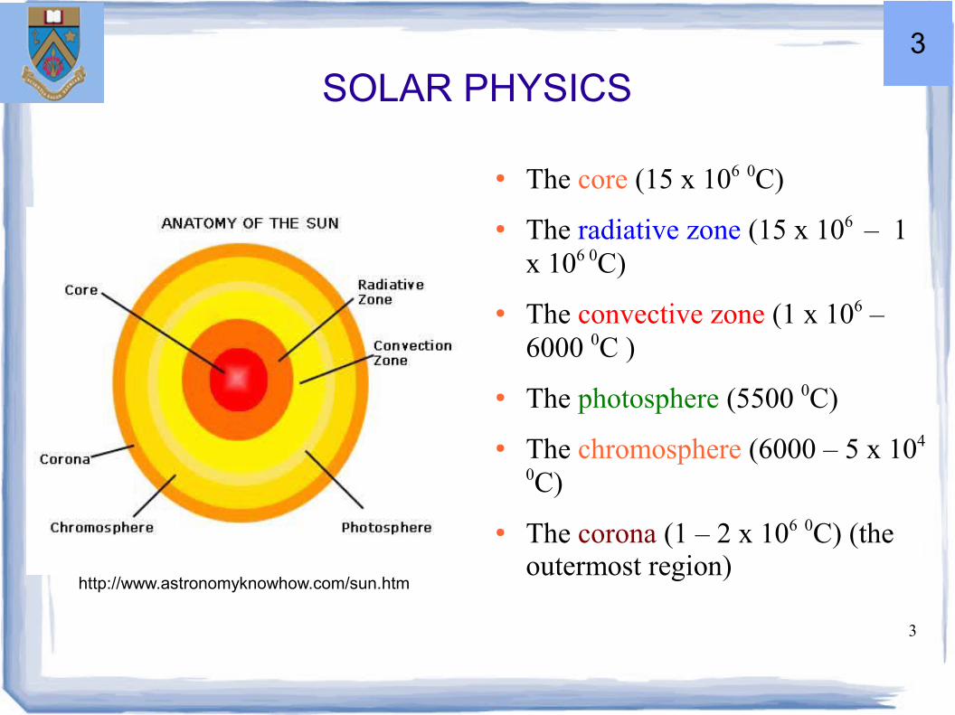
SOLAR PHYSICS

● The core (15 x 106 0C)

● The radiative zone (15 x 106 – 1 x 106 0C)

● The convective zone (1 x 106 – 6000 0C )

● The photosphere (5500 0C)

● The chromosphere (6000 – 5 x 104 0C)

● The corona (1 – 2 x 106 0C) (the outermost region)

http://www.astronomyknowhow.com/sun.htm

3

4

THE CORONA

● Final layer of the three regions that make up the sun's atmosphere.

● Widest region of sun's atmosphere.

● Extends over several million kilometres from the photosphere and chromosphere.

● ~ 2 million degrees Kelvin, and hottest layer of Sun.

● Best seen in X-ray images and during solar eclipses.

http://www.qrg.northwestern.edu/projects/vss/docs/space-environment/3-what-is-solar-wind.html

4

5

HEATING PROBLEM OF THE CORONA

● The temperature should decrease with height above the Sun. Instead, it increases.

● For this high temperature to exist, there must be a permanent heating mechanism.

● Complex Magneto-hydro-dynamic (MHD) problem

● Two theories for the heating mechanism:

1. Wave heating theory

2. Magnetic reconnection theory

5

SOLAR FLARES

6

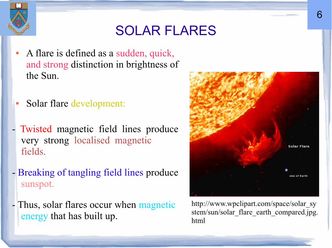
● A flare is defined as a sudden, quick, and strong distinction in brightness of the Sun.

● Solar flare development:

- Twisted magnetic field lines produce very strong localised magnetic fields.

- Breaking of tangling field lines produce sunspot.

- Thus, solar flares occur when magnetic energy that has built up.

http://www.wpclipart.com/space/solar_system/sun/solar_flare_earth_compared.jpg.html

6

CLASSIFICATION OF SOLAR FLARES

Five types of flare importance classification are known:

H-alpha importance (scale 0-3)Here, we observe the behavior of the Sun's in the mid

chromosphere.

10.7 cm solar radio flux magnitude

Solar Radio Spectral Type

Magnitude of 200 MHz flux

Sudden Ionospheric Disturbance importance (scale 0-3)7

7

8

● Compound

● Astronomical

● Low-Cost

● Low-Frequency

● Instrument for

● Spectroscopy &

● Transportable

● Observatory

CALLISTO: The e-CALLISTO Map Coverage (28 active stations):

THE CALLISTO

http://www.astro.phys.ethz.ch/astro1/Users/cmonstei/instrument/callisto/Callisto_World.png

8

9

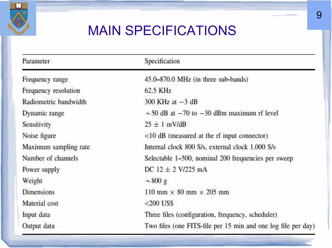
MAIN SPECIFICATIONS 9

HOW DOES THE SPECTROMETER WORK? I

antenna

RF Input

Dc power coaxial connector

EIA-232 Interface

10

● Signals from the feed are fed into the receivers.

● They convert to a first intermediate frequency of 37.7 MHz by two local oscillators.

● The signal is down converted to 10.7 MHz for filtering and amplification, detected by logarithmic device, and low pass filtered.

● The logarithmic domain is more than 45 db.

HOW DOES THE SPECTROMETER WORK? II

11

● Data acquisition for both receivers and the interface to the PC are on a separate board.

● The measurements are made in a two step process.

● In the first step a receiver is tuned to a frequency, in the second step the signal is measured.

● The receivers can also be configured to measure the same polarization and to alternate: while one is measuring, the other is tuned to a new frequency.

HOW DOES THE SPECTROMETER WORK? III

12

FITS FILE HEADER13

TYPES OF FLARES

● Type I

– Duration: Seconds

– Freq. Range : 80 – 200 MHz

Circular pol: Bleinen 7 m Linear pol: Ooty

14

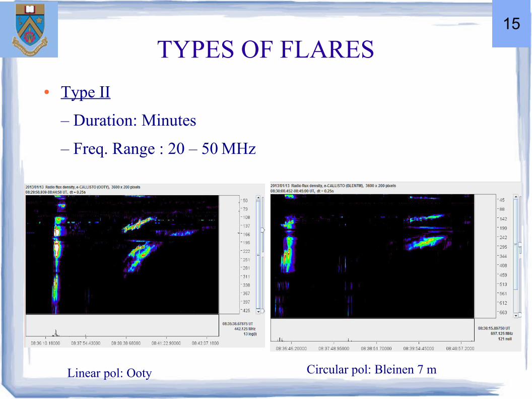
TYPES OF FLARES

● Type II

– Duration: Minutes

– Freq. Range : 20 – 50 MHz

Circular pol: Bleinen 7 m Linear pol: Ooty

15

TYPES OF FLARES

● Type III

– Duration: Seconds or Hours

– Freq. Range :10 KHz – 1 GHz

Circular pol: Bleinen 7 m Linear pol: Gauri

16

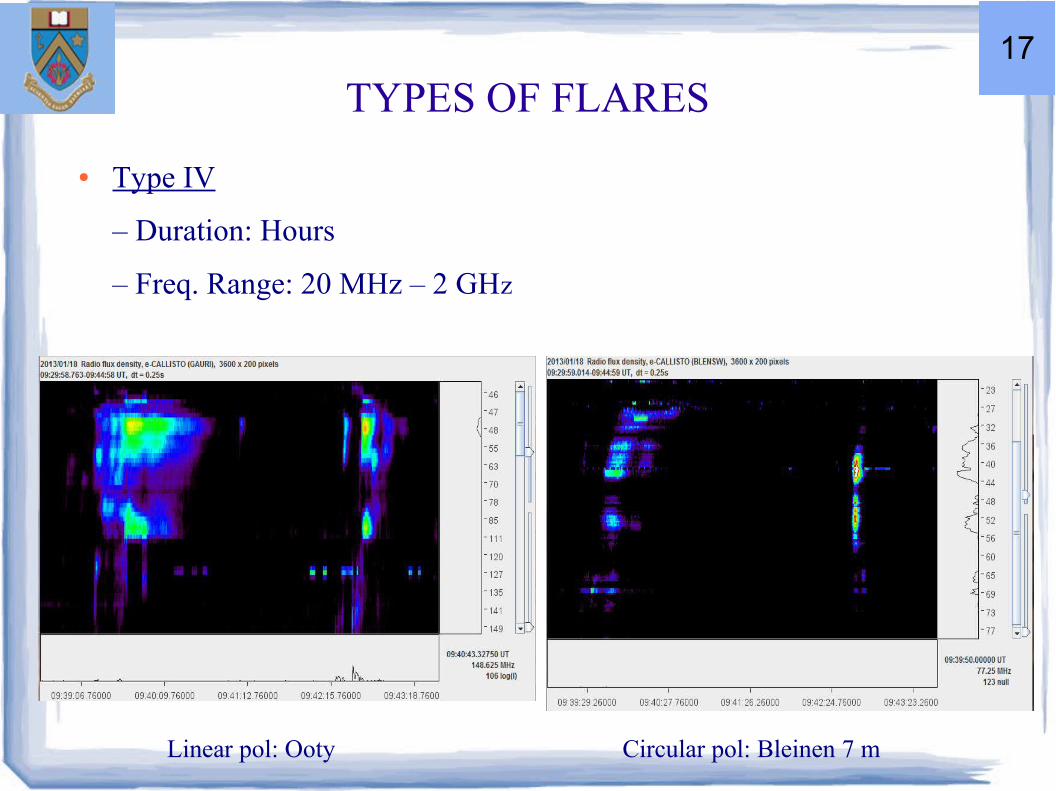
TYPES OF FLARES

● Type IV

– Duration: Hours

– Freq. Range: 20 MHz – 2 GHz

Circular pol: Bleinen 7 m Linear pol: Ooty

17

18

● Type V

– Duration: Hours

– Freq. Range : 10 MHz – 20 MHz

TYPES OF FLARES

Circular pol: Bleinen 7 m Linear pol: Ooty

18

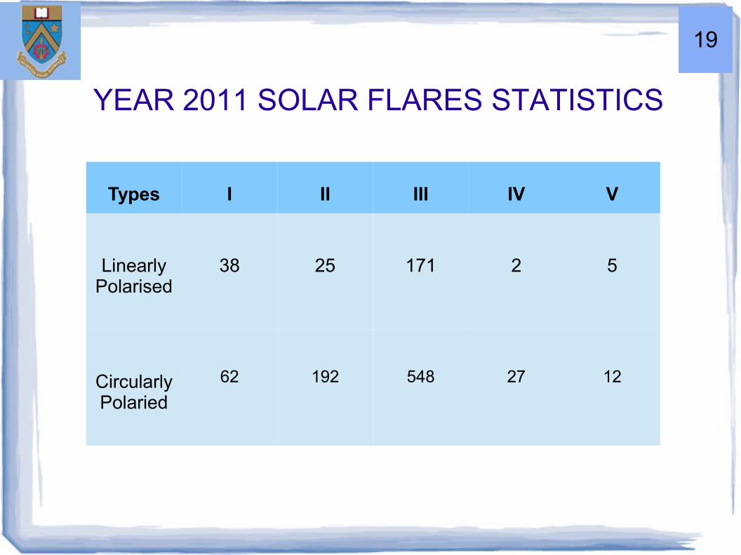
Types I II III IV V

Linearly Polarised

38 25 171 2 5

Circularly Polaried

62 192 548 27 12

YEAR 2011 SOLAR FLARES STATISTICS

19

20

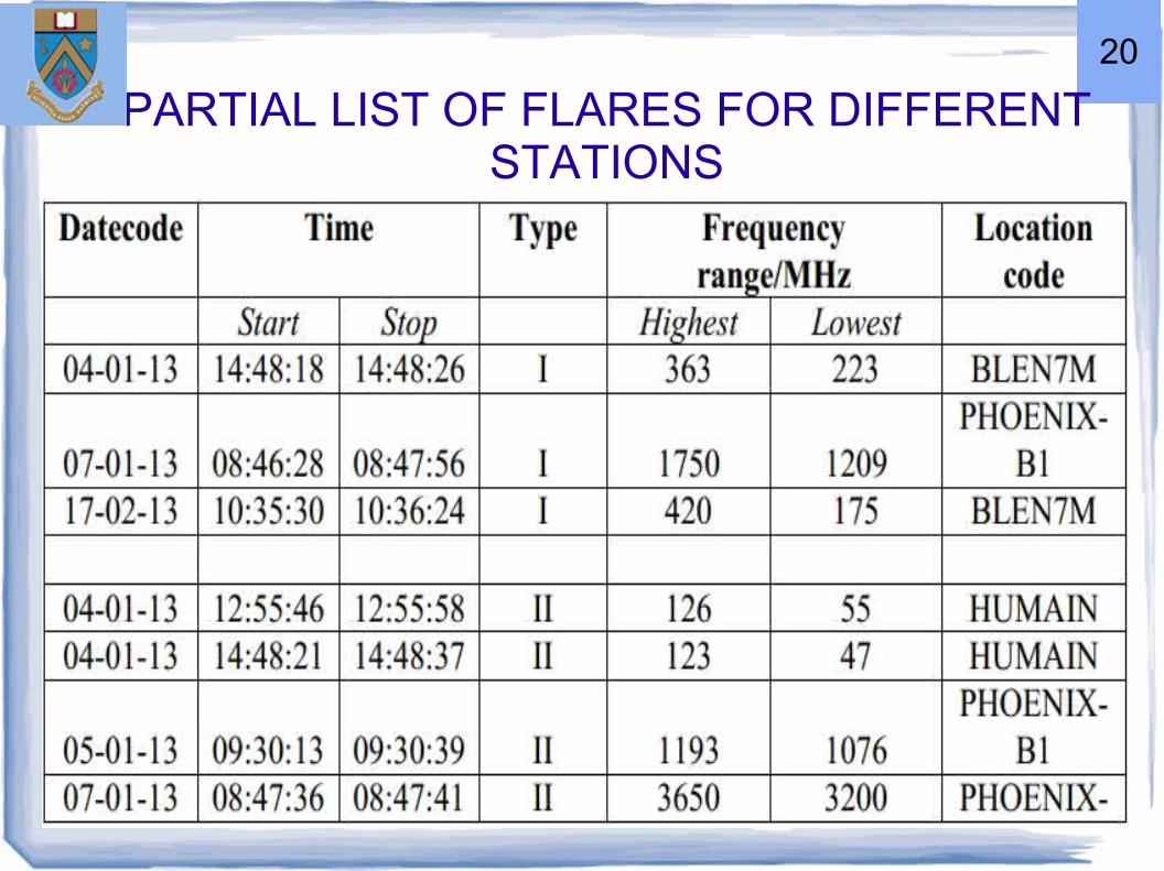
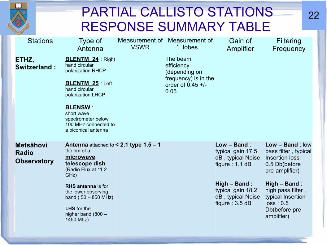
PARTIAL LIST OF FLARES FOR DIFFERENT STATIONS

CALLISTO STATIONS

All stations were contacted for information. Only 15 responded. The following facts were gleaned:

the type of antenna used.

any measurement of VSWR.

any measurement of main & side lobes.

the net gain of amplifiers.

the frequency filtering, if used.21

21

Stations Type of Antenna

Measurement of VSWR

Measurement of lobes

Gain of Amplifier

Filtering Frequency

ETHZ, Switzerland :

BLEN7M_24 : Right hand circular polarization RHCP

BLEN7M_25 : Left hand circular polarization LHCP

BLENSW :short wave spectrometer below 100 MHz connected to a biconical antenna

The beam efficiency (depending on frequency) is in the order of 0.45 +/- 0.05

Metsähovi Radio Observatory

Antenna attached to the rim of a microwave telescope dish(Radio Flux at 11.2 GHz)

RHS antenna is for the lower observing band ( 50 – 850 MHz)

LHS for the higher band (800 – 1450 Mhz)

< 2.1 type 1.5 – 1 Low – Band : typical gain 17.5 dB , typical Noise figure : 1.1 dB

High – Band : typical gain 18.2 dB , typical Noise figure : 3.5 dB

Low – Band : low pass filter , typical Insertion loss : 0.5 Db(before pre-amplifier)

High – Band : high pass filter , typical Insertion loss : 0.5 Db(before pre-amplifier)

PARTIAL CALLISTO STATIONS RESPONSE SUMMARY TABLE

:

22

ANALYSIS OF SOLAR DATA USING SUNPY

● SunPy is a free and open-source software.

● It uses Python programing language.

● It builds upon science packages available for Python including NumPy, SciPy and matplotlib.

● Programs were written for data analysis using this software.

23

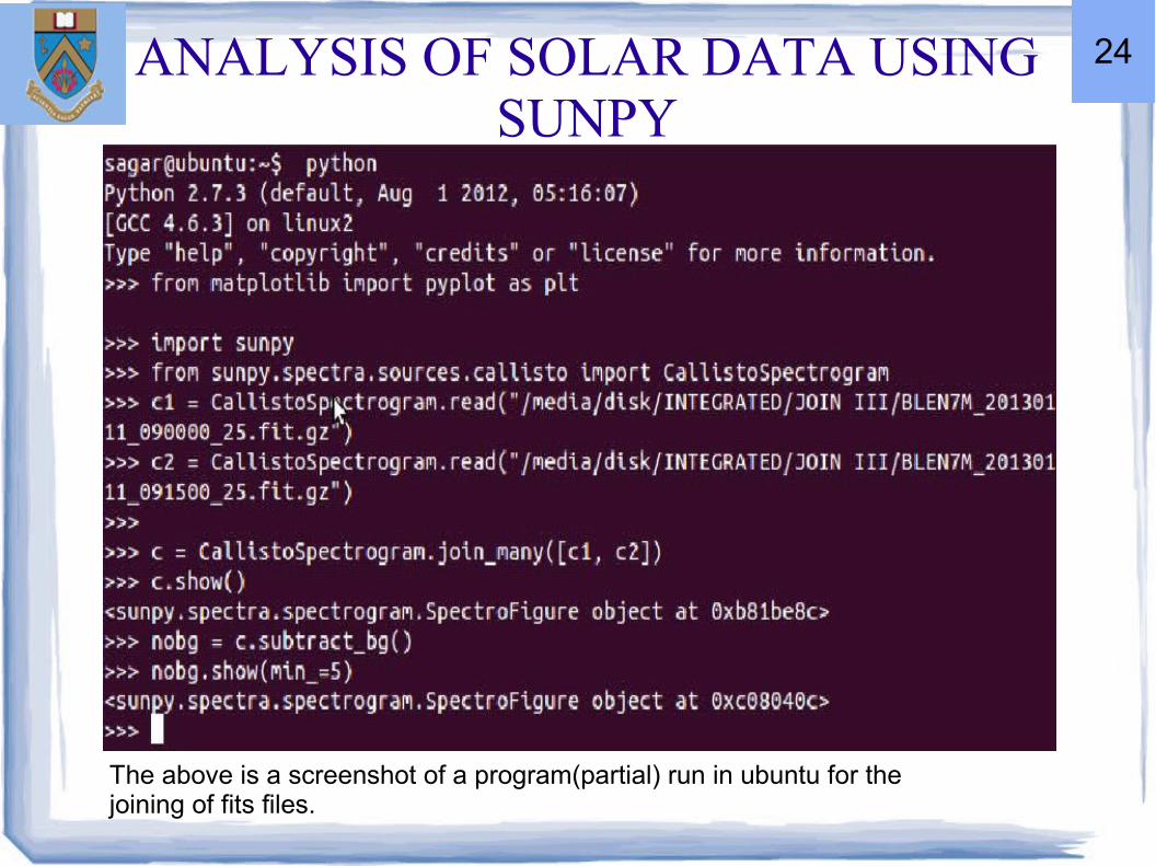
ANALYSIS OF SOLAR DATA USING SUNPY

The above is a screenshot of a program(partial) run in ubuntu for the joining of fits files.

24

DATA ANALYSIS FOR LINEAR POLARISED ANTENNAS

25

26

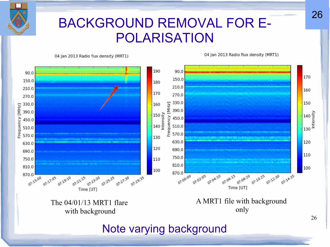
BACKGROUND REMOVAL FOR E-POLARISATION

The 04/01/13 MRT1 flare with background

A MRT1 file with background only

Note varying background

26

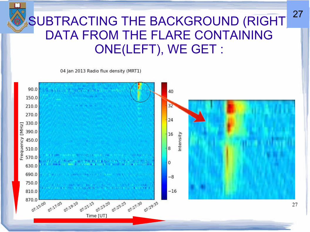
27

SUBTRACTING THE BACKGROUND (RIGHT) DATA FROM THE FLARE CONTAINING

ONE(LEFT), WE GET :

27

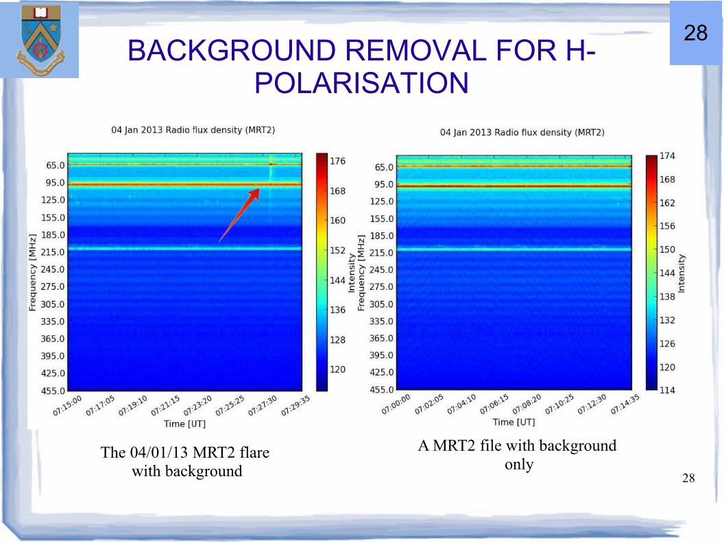
28

BACKGROUND REMOVAL FOR H-POLARISATION

The 04/01/13 MRT2 flare with background

A MRT2 file with background only

28

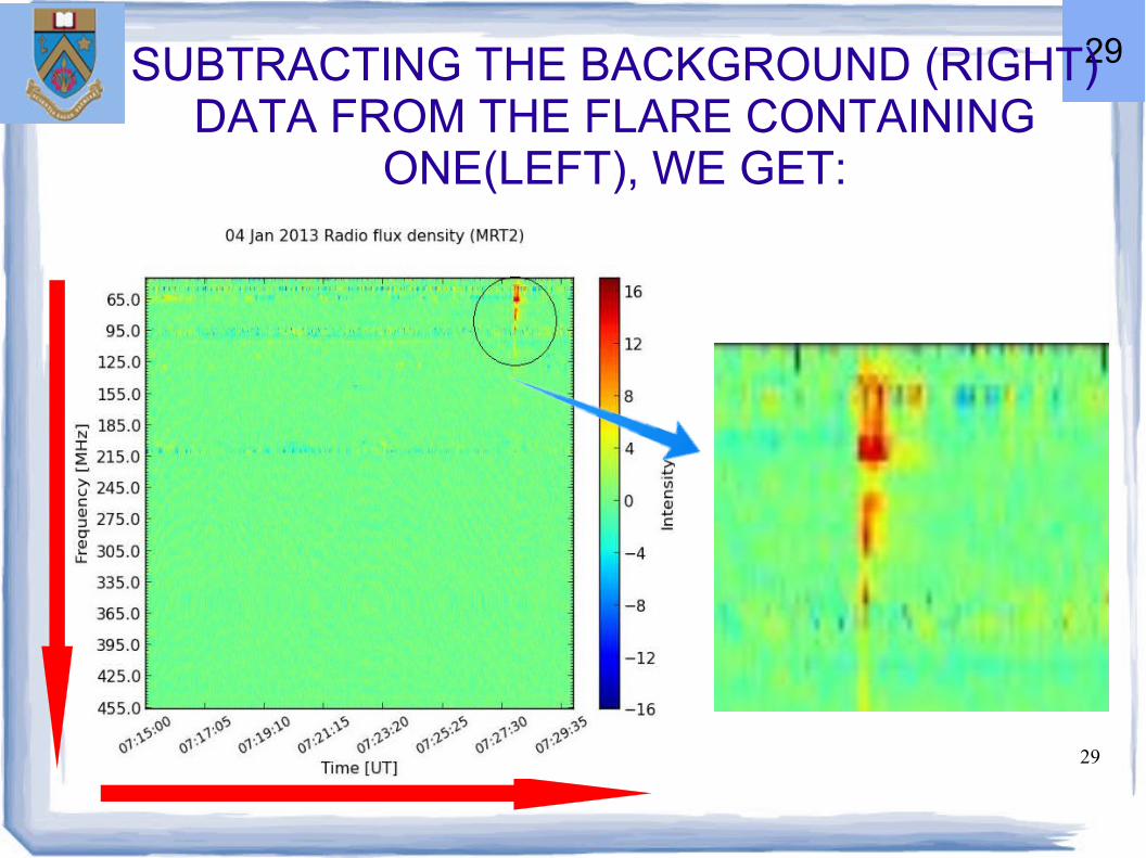
29

29SUBTRACTING THE BACKGROUND (RIGHT) DATA FROM THE FLARE CONTAINING

ONE(LEFT), WE GET:

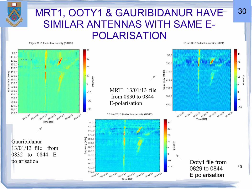
30

MRT1, OOTY1 & GAURIBIDANUR HAVE SIMILAR ANTENNAS WITH SAME E-

POLARISATION

Gauribidanur 13/01/13 file from 0832 to 0844 E-polarisation

MRT1 13/01/13 file from 0830 to 0844E-polarisation

Ooty1 file from 0829 to 0844 E polarisation

30

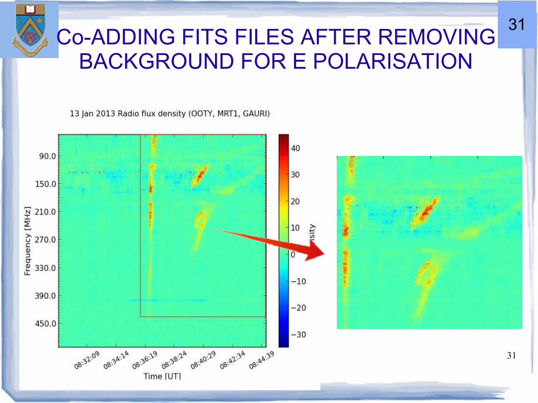
31

31Co-ADDING FITS FILES AFTER REMOVING

BACKGROUND FOR E POLARISATION

32

JOINING FITS FILES IN TIME

The two consecutive 15 min files were joined after subtraction of background:

A B

32

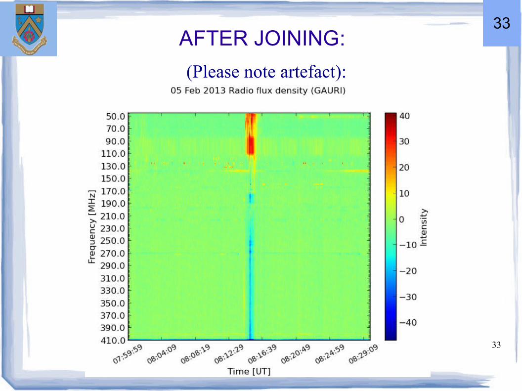
33

AFTER JOINING:

(Please note artefact):

33

DATA ANALYSIS FOR CIRCULAR POLARISED ANTENNAS

34

FLARE OBSERVED AT BLENSW

The Blensw with flare and background

The Blensw with background only

35

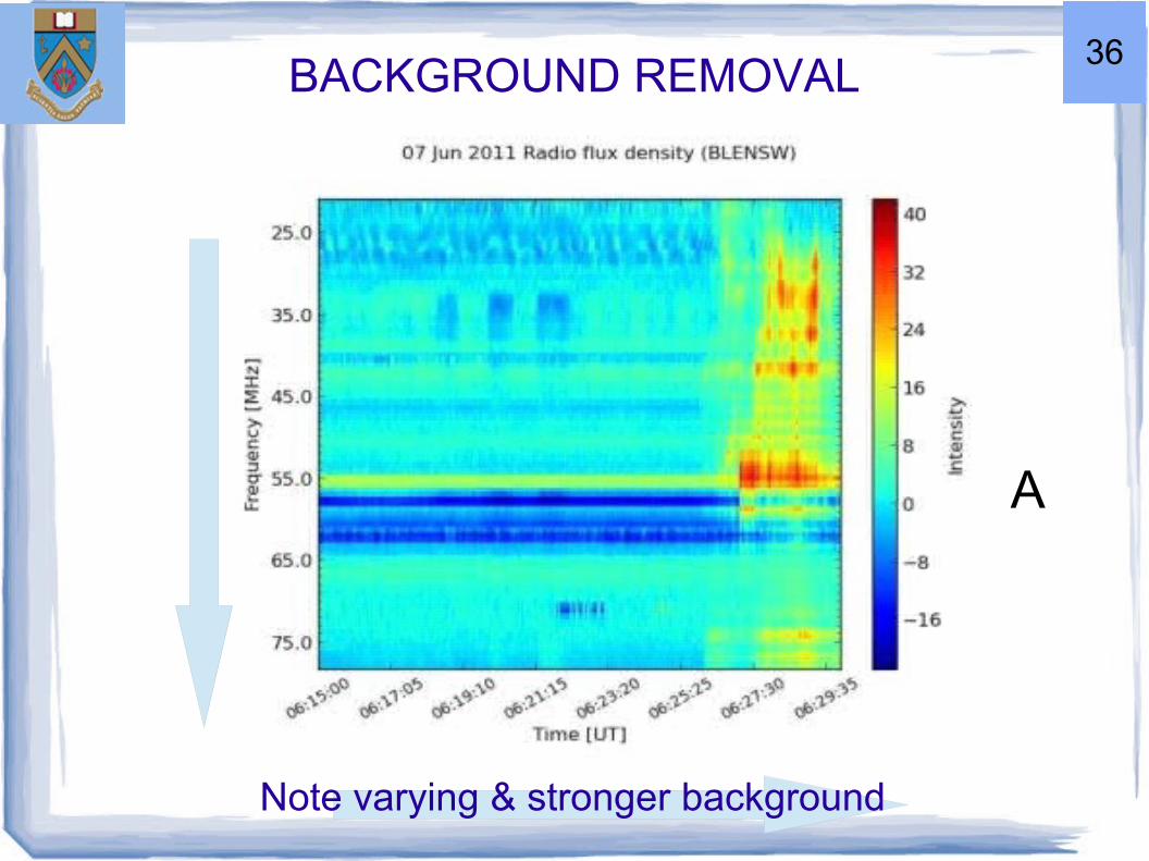
BACKGROUND REMOVAL

A

Note varying & stronger background

36

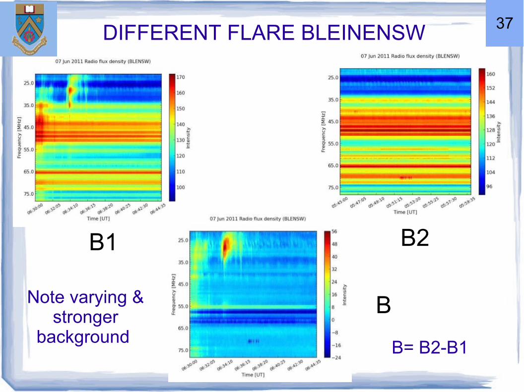
B

DIFFERENT FLARE BLEINENSW

B2B1

Note varying & stronger

background B= B2-B1

37

After joining the two BLENSW, the timescale is from 06:15 to 06: 45

JOINING A AND B IN TIME38

SAME FLARE FOR HUMAIN

C

39

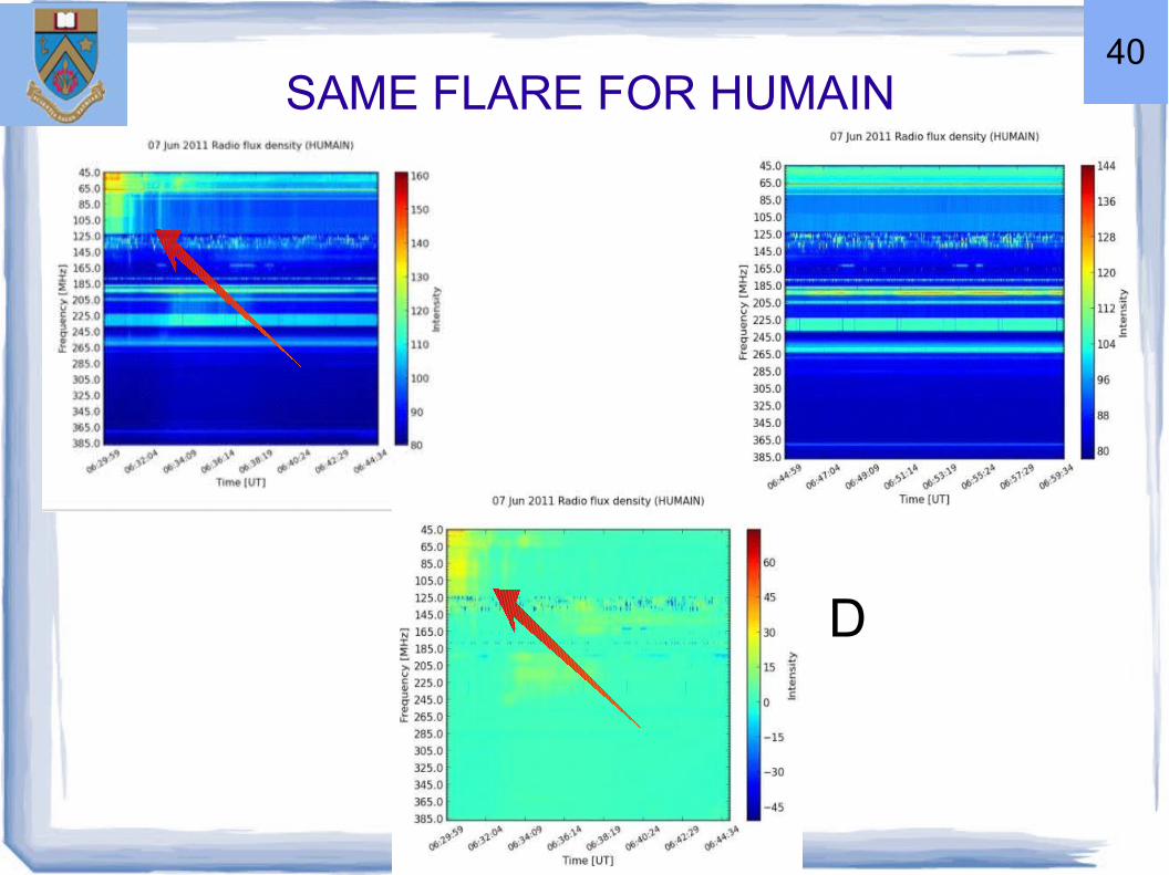
D

40SAME FLARE FOR HUMAIN

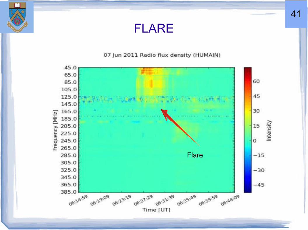
Flare

FLARE41

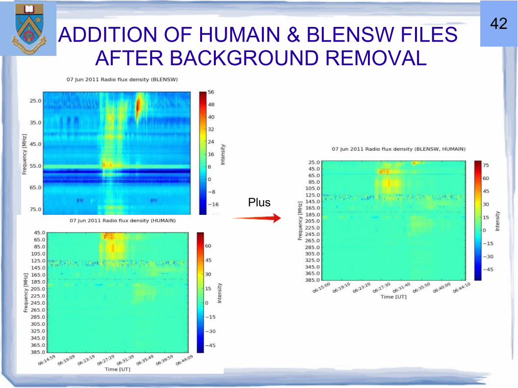
42

Plus

ADDITION OF HUMAIN & BLENSW FILES AFTER BACKGROUND REMOVAL

ADDITION OF BLEN7M & HUMAIN 43

CORONAL MASS EJECTIONS

● Strong and energetic outbursts occurring on the Sun's surface.

● Controlled by strong magnetic fields.

● Due to instabilities in the magnetic field of the Sun, the

restricted solar atmosphere abruptly eject heated bubbles of

gas, i.e. the CMEs.

● With the MITRA antenna recently constructed at the MRT, a 2

hour long CME was observed on the 15th March 2013.

44

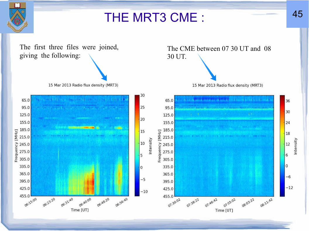
The first three files were joined, giving the following:

45

The CME between 07 30 UT and 08 30 UT.

THE MRT3 CME : 45

The first 3 files from 0615 to 0700

THE CME OBSERVED BY BLEN7M

The CME between 0730 to 0830

47

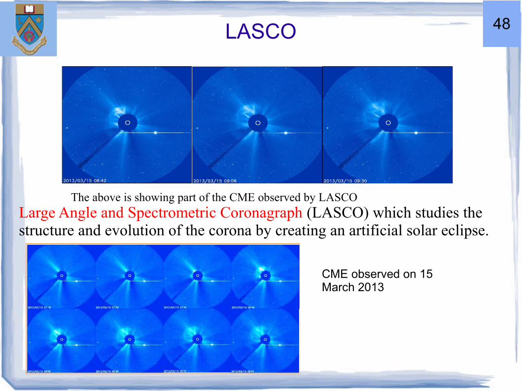
The above is showing part of the CME observed by LASCO

Large Angle and Spectrometric Coronagraph (LASCO) which studies the structure and evolution of the corona by creating an artificial solar eclipse.

CME observed on 15 March 2013

48LASCO

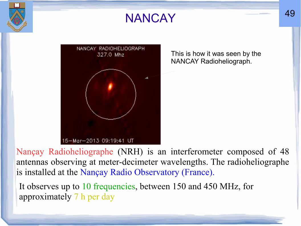
This is how it was seen by the NANCAY Radioheliograph.

It observes up to 10 frequencies, between 150 and 450 MHz, for approximately 7 h per day

Nançay Radioheliographe (NRH) is an interferometer composed of 48 antennas observing at meter-decimeter wavelengths. The radioheliographe is installed at the Nançay Radio Observatory (France).

49NANCAY

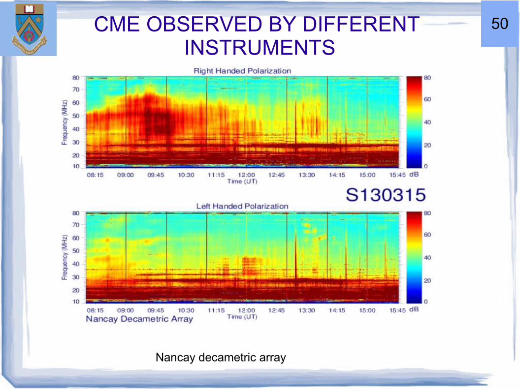
50CME OBSERVED BY DIFFERENT INSTRUMENTS

Nancay decametric array

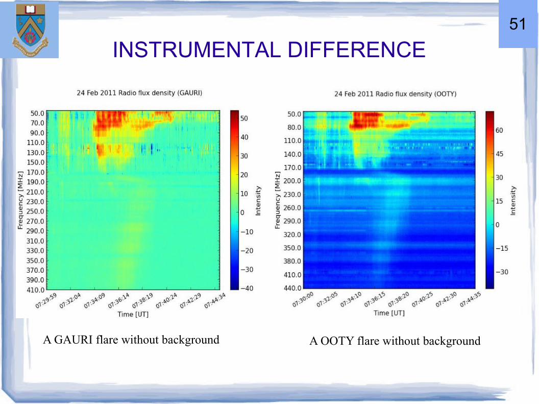
50A GAURI flare without background A OOTY flare without background

INSTRUMENTAL DIFFERENCE51

51

This graph was obtained by subtracting the GAURI file from the OOTY one.

THE DIFFERENCE BETWEEN THE PREVIOUS FILES

52

DIFFERENCE BETWEEN THE BACKGROUNDS OF GAURI & MRT1 FLARE

53

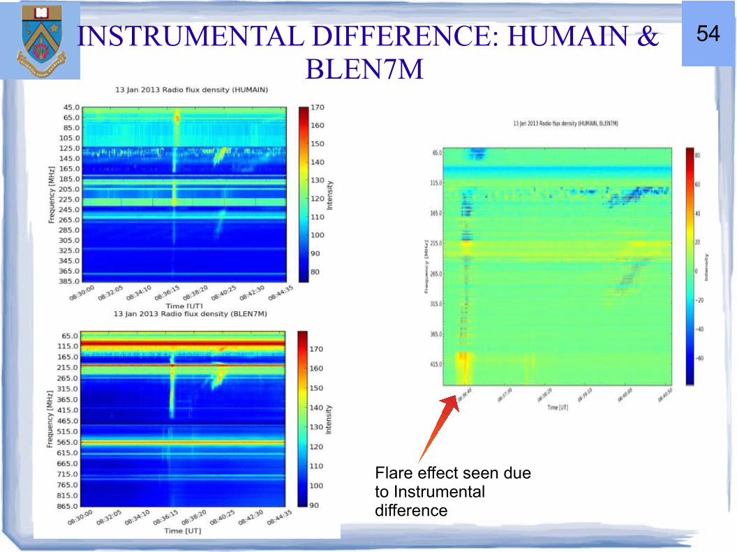
Flare effect seen due to Instrumental difference

INSTRUMENTAL DIFFERENCE: HUMAIN & BLEN7M

54

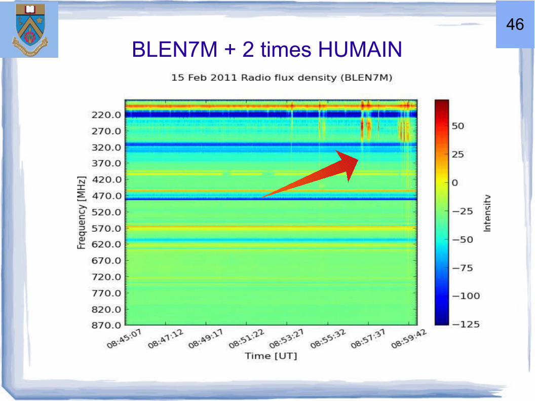
BLEN7M + 2 times HUMAIN46

WEAK BURSTS IN THE SOLAR CORONA IN ABSENCE OF X RAY EMISSION

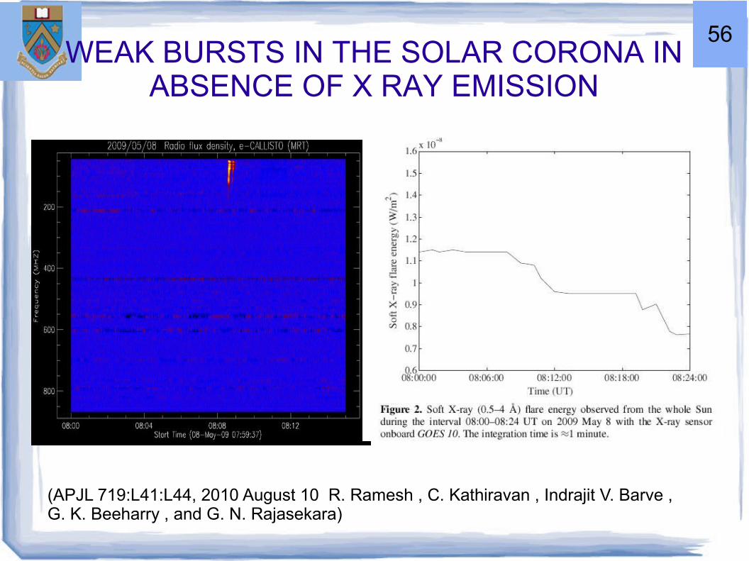
● Observations of weak, circularly polarized, structureless type III bursts from the solar corona (in absence of H/X-ray flares and other related activity).

● CALLISTO Mauritius: ● emission from 50 to 120 MHz & drift rate ~ -30 Mhz/s

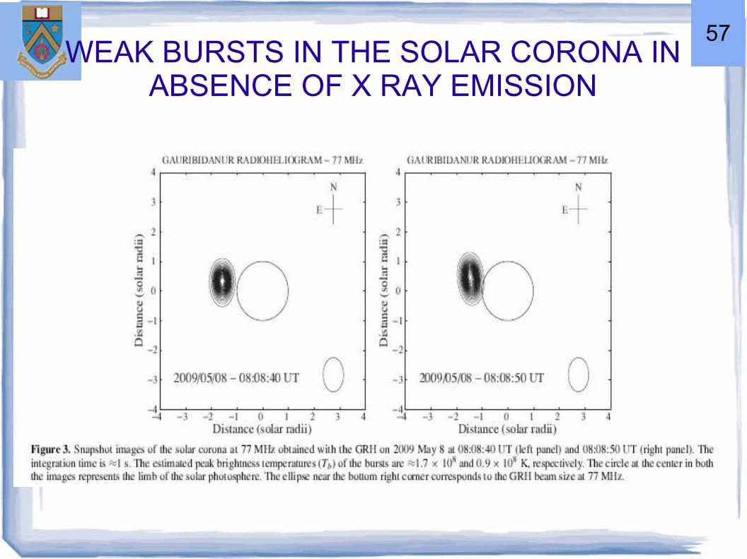
● Imaging 2-D data from Gauribidanur radioheliograph at 77 MHz: burst at 1.5 Ro in solar atmosphere

● Gauribidanur East-West polarimeter: magnetic field ~2.5G

● Energy of non thermal electrons ~1.1x1024 ergs (X-ray nicroflare ~ 1026 ergs). Nature unknown.

(APJL 719:L41:L44, 2010 August 10 R. Ramesh , C. Kathiravan , Indrajit V. Barve , G. K. Beeharry , and G. N. Rajasekara)

55

WEAK BURSTS IN THE SOLAR CORONA IN ABSENCE OF X RAY EMISSION

(APJL 719:L41:L44, 2010 August 10 R. Ramesh , C. Kathiravan , Indrajit V. Barve , G. K. Beeharry , and G. N. Rajasekara)

56

WEAK BURSTS IN THE SOLAR CORONA IN ABSENCE OF X RAY EMISSION

57

CONCLUSION & FUTURE WORK

The data analysis of flares and CMEs has been successfully

carried out using a new technique. This work will be furthered by

the following improvements in the algorithms:

● Using the detail antenna patterns to correct for the flares in CME emissions.

● In optimizing techniques to combine data from different instruments with similar antenna patterns.

● In developing new techniques to use data from different instrument with dissimilar antenna patterns.

● Flux calibration for each instrument.

● Correction for instrumental effect in spectrum.

58

REFERENCES

●http://itsabeautifulearth.com/2013/02/23/nasas-solar-dynamics-observatory-

captures-beautiful-solar-flare/

●A World-Wide Net of Solar Radio Spectrometers: e-CALLISTO

●http://www.e-callisto.org

●http://sohodata.nascom.nasa.gov/cgi-bin/data_query

●http://bass2000.obspm.fr/search.php?step=2

59