
OBSERVATIONS FROM LOAD TESTS ON GEOSYNTHETIC REINFORCED SOIL
Upload
iqbal-aamerCategory
view
130download
6description
ENGINEERING PROPERTIES OF SOILS
BASED ON LABORATORY TESTING
Krishna R. Reddy, Ph.D., P.E. Associate Professor of Civil & Environmental Engineering
Director of Geotechnical and Geoenvironmental Engineering Laboratory Tel: (312)996-4755; Fax: (312)996-2426; e-mail: [email protected]
Department of Civil and Materials Engineering University of Illinois at Chicago
August 2002

Engineering Properties of Soils Based on Laboratory Testing Prof. Krishna Reddy, UIC
1
INTRODUCTION
Soil is one of the most important engineering materials. Determination of soil
conditions is the most important first phase of work for every type of civil
engineering facility. Soil properties are determined by both field and laboratory test
methods. In this course, you will learn several laboratory tests that are very
commonly performed to determine different properties of soils. These properties
are essential for the design of foundation and earth structures.
In this course, different laboratory tests will be conducted to determine the
following important index and mechanical properties of soils:
• Water Content
• Organic Matter (Content)
• Unit Weight (Density)
• Specific Gravity
• Relative Density
• Atterberg Limits
• Grain Size Distribution (Sieve Analysis and Hydrometer Analysis)
• Visual Classification
• Moisture-Density Relationship (Compaction)
• Hydraulic Conductivity (Constant Head Method)
• Consolidation
• Shear Strength
o Unconfined Compression Test
o Direct Shear Test
Engineering Properties of Soils Based on Laboratory Testing Prof. Krishna Reddy, UIC
2
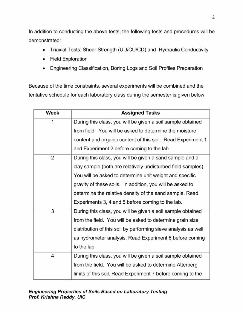
In addition to conducting the above tests, the following tests and procedures will be
demonstrated:
• Triaxial Tests: Shear Strength (UU/CU/CD) and Hydraulic Conductivity
• Field Exploration
• Engineering Classification, Boring Logs and Soil Profiles Preparation
Because of the time constraints, several experiments will be combined and the
tentative schedule for each laboratory class during the semester is given below:
Week Assigned Tasks
1 During this class, you will be given a soil sample obtained
from field. You will be asked to determine the moisture
content and organic content of this soil. Read Experiment 1
and Experiment 2 before coming to the lab.
2 During this class, you will be given a sand sample and a
clay sample (both are relatively undisturbed field samples).
You will be asked to determine unit weight and specific
gravity of these soils. In addition, you will be asked to
determine the relative density of the sand sample. Read
Experiments 3, 4 and 5 before coming to the lab.
3 During this class, you will be given a soil sample obtained
from the field. You will be asked to determine grain size
distribution of this soil by performing sieve analysis as well
as hydrometer analysis. Read Experiment 6 before coming
to the lab.
4 During this class, you will be given a soil sample obtained
from the field. You will be asked to determine Atterberg
limits of this soil. Read Experiment 7 before coming to the
Engineering Properties of Soils Based on Laboratory Testing Prof. Krishna Reddy, UIC
3
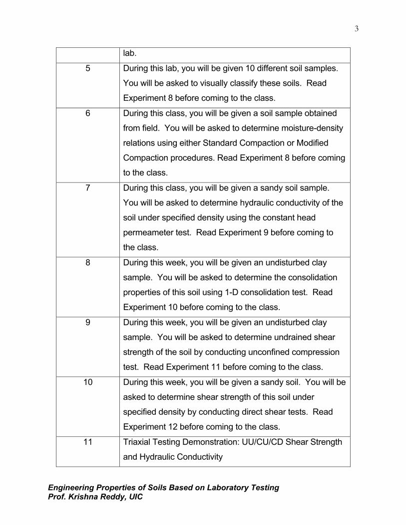
lab.
5 During this lab, you will be given 10 different soil samples.
You will be asked to visually classify these soils. Read
Experiment 8 before coming to the class.
6 During this class, you will be given a soil sample obtained
from field. You will be asked to determine moisture-density
relations using either Standard Compaction or Modified
Compaction procedures. Read Experiment 8 before coming
to the class.
7 During this class, you will be given a sandy soil sample.
You will be asked to determine hydraulic conductivity of the
soil under specified density using the constant head
permeameter test. Read Experiment 9 before coming to
the class.
8 During this week, you will be given an undisturbed clay
sample. You will be asked to determine the consolidation
properties of this soil using 1-D consolidation test. Read
Experiment 10 before coming to the class.
9 During this week, you will be given an undisturbed clay
sample. You will be asked to determine undrained shear
strength of the soil by conducting unconfined compression
test. Read Experiment 11 before coming to the class.
10 During this week, you will be given a sandy soil. You will be
asked to determine shear strength of this soil under
specified density by conducting direct shear tests. Read
Experiment 12 before coming to the class.
11 Triaxial Testing Demonstration: UU/CU/CD Shear Strength
and Hydraulic Conductivity

Engineering Properties of Soils Based on Laboratory Testing Prof. Krishna Reddy, UIC
4
12 Field Exploration Methods-Demonstration
13 Engineering Classification, Boring Logs and Soil Profiles-
Practice Examples
A short report which details the weekly experiment will be due 1 (one) week
after the completion of the lab. You will work in teams, but everyone must submit
an individual report. The body of each lab report shall consist of no more than
three 8-1/2 x 11 pages of typed text. Any text beyond the first three pages shall be
disregarded, so be concise! As many figures as deemed necessary can
accompany the 3 pages of text in the report body. All raw data and calculations
should be appended to the body of the report. Remember neatness counts.
Prepare your report according to the format shown below.
I. Introduction Include: (1) brief description of what you did
in lab and (2) the purpose of the lab.
II. Procedures Read the ASTM standard for the test(s) you
conducted and note any differences
between ASTM recommended procedure(s)
and the procedure(s) that actually used in
the lab.
III. Results Present the results of the lab in this section.
Refer to figures or tables when necessary.
IV. Discussion Describe your results. Do they seem
reasonable? Include analyses of possible
errors and any recommendations that you
have for improving the test procedure.

Engineering Properties of Soils Based on Laboratory Testing Prof. Krishna Reddy, UIC
5
V. Conclusions Draw your conclusions and present them in
this section.
. Tables (in order)
. Figures (in order)
APPENDIX: Include raw data and calculations in Appendix.
NOTES: 1. You must refer to each Table and Figure in the TEXT.
2. Remember that Sections I-V can only be a maximum of three 8-
1/2 x 11 in. pages in length. So be concise (this does not mean
to omit anything).

Engineering Properties of Soils Based on Laboratory Testing Prof. Krishna Reddy, UIC
6
EXPERIMENT 1 WATER CONTENT DETERMINATION
Purpose: This test is performed to determine the water (moisture) content of soils. The
water content is the ratio, expressed as a percentage, of the mass of “pore” or
“free” water in a given mass of soil to the mass of the dry soil solids.
Standard Reference:
ASTM D 2216 - Standard Test Method for Laboratory Determination of
Water (Moisture) Content of Soil, Rock, and Soil-Aggregate Mixtures
Significance:
For many soils, the water content may be an extremely important index used
for establishing the relationship between the way a soil behaves and its properties.
The consistency of a fine-grained soil largely depends on its water content. The
water content is also used in expressing the phase relationships of air, water, and
solids in a given volume of soil.
Equipment: Drying oven, Balance, Moisture can, Gloves, Spatula.

Engineering Properties of Soils Based on Laboratory Testing Prof. Krishna Reddy, UIC
7
Engineering Properties of Soils Based on Laboratory Testing Prof. Krishna Reddy, UIC
8
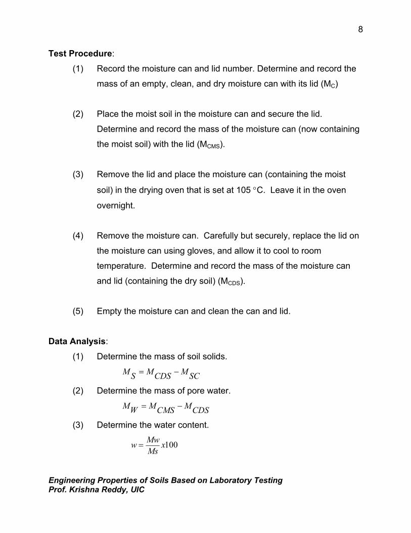
Test Procedure: (1) Record the moisture can and lid number. Determine and record the
mass of an empty, clean, and dry moisture can with its lid (MC)
(2) Place the moist soil in the moisture can and secure the lid.
Determine and record the mass of the moisture can (now containing
the moist soil) with the lid (MCMS).
(3) Remove the lid and place the moisture can (containing the moist
soil) in the drying oven that is set at 105 °C. Leave it in the oven
overnight.
(4) Remove the moisture can. Carefully but securely, replace the lid on
the moisture can using gloves, and allow it to cool to room
temperature. Determine and record the mass of the moisture can
and lid (containing the dry soil) (MCDS).
(5) Empty the moisture can and clean the can and lid.
Data Analysis:
(1) Determine the mass of soil solids.
SCMCDSMSM −=
(2) Determine the mass of pore water.
CDSMCMSMWM −=
(3) Determine the water content.
100xMsMww =
Engineering Properties of Soils Based on Laboratory Testing Prof. Krishna Reddy, UIC
9
EXAMPLE DATA

Engineering Properties of Soils Based on Laboratory Testing Prof. Krishna Reddy, UIC
10
WATER CONTENT DETERMINATION
DATA SHEET
Date Tested: August 30, 2002 Tested By: CEMM315 Class, Group A
Project Name: CEMM315 Lab
Sample Number: B-1,AU-1, 0’-2’
Sample Description: Gray silty clay
Specimen number 1 2
Moisture can and lid number 12 15
MC = Mass of empty, clean can + lid (grams) 7. 78 7.83
MCMS = Mass of can, lid, and moist soil (grams) 16. 39 13.43
MCDS = Mass of can, lid, and dry soil (grams) 15. 28 12.69
MS = Mass of soil solids (grams) 7. 5 4.86
MW = Mass of pore water (grams) 1 . 11 0.74
w = Water content, w% 14.8 15. 2
Example Calculation: MC = 7.78g, MCMS = 16.39g, MCDS = 15.28g
MS = 15.28 – 7.78 = 7.5g
MW = 16.39 -15.28 = 1.11g
x1007.5
1.11w = = 14.8%

Engineering Properties of Soils Based on Laboratory Testing Prof. Krishna Reddy, UIC
11
BLANK DATA SHEETS

Engineering Properties of Soils Based on Laboratory Testing Prof. Krishna Reddy, UIC
12
WATER CONTENT DETERMINATION
DATA SHEET
Date Tested: Tested By: Project Name: Sample Number: Sample Description:
Specimen number 1 2 Moisture can and lid number MC = Mass of empty, clean can + lid (grams) MCMS = Mass of can, lid, and moist soil (grams) MCDS = Mass of can, lid, and dry soil (grams) MS = Mass of soil solids (grams) MW = Mass of pore water (grams) w = Water content, w%

Engineering Properties of Soils Based on Laboratory Testing Prof. Krishna Reddy, UIC
13
EXPERIMENT 2 ORGANIC MATTER DETERMINATION
Purpose: This test is performed to determine the organic content of soils. The
organic content is the ratio, expressed as a percentage, of the mass of
organic matter in a given mass of soil to the mass of the dry soil solids.
Standard Reference: ASTM D 2974 – Standard Test Methods for Moisture, Ash, and
Organic Matter of Peat and Organic Soils
Significance: Organic matter influences many of the physical, chemical and
biological properties of soils. Some of the properties influenced by organic
matter include soil structure, soil compressibility and shear strength. In
addition, it also affects the water holding capacity, nutrient contributions,
biological activity, and water and air infiltration rates.
Equipment: Muffle furnace, Balance, Porcelain dish, Spatula, Tongs

Engineering Properties of Soils Based on Laboratory Testing Prof. Krishna Reddy, UIC
14
Test Procedure:
(1) Determine and record the mass of an empty, clean, and dry
porcelain dish (MP).
(2) Place a part of or the entire oven-dried test specimen from the
moisture content experiment (Expt.1) in the porcelain dish and
determine and record the mass of the dish and soil specimen
(MPDS).
(3) Place the dish in a muffle furnace. Gradually increase the
temperature in the furnace to 440oC. Leave the specimen in
the furnace overnight.
(4) Remove carefully the porcelain dish using the tongs (the dish
is very hot), and allow it to cool to room temperature.

Engineering Properties of Soils Based on Laboratory Testing Prof. Krishna Reddy, UIC
15
Determine and record the mass of the dish containing the ash
(burned soil) (MPA).
(5) Empty the dish and clean it.
Data Analysis:
(1) Determine the mass of the dry soil.
MD=MPDS-MP
(2) Determine the mass of the ashed (burned) soil.
MA=MPA-MP
(3) Determine the mass of organic matter
MO = MD - MA
(4) Determine the organic matter (content).
100xMM
OMD
O=
Engineering Properties of Soils Based on Laboratory Testing Prof. Krishna Reddy, UIC
16
EXAMPLE DATA

Engineering Properties of Soils Based on Laboratory Testing Prof. Krishna Reddy, UIC
17
ORGANIC MATTER DETERMINATION DATA SHEET
Date Tested: August 30, 2002 Tested By: CEMM315 Class, Group A
Project Name: CEMM315 Lab
Sample Number: B-1,AU-1, 0’-2’
Sample Description: Gray silty clay
Specimen number 1 2
Porcelain dish number 5 8
MP = Mass of empty, clean porcelain dish (grams) 23.20 23.03
MPDS = Mass of dish and dry soil (grams) 35.29 36.66
MPA = Mass of the dish and ash (Burned soil) (grams) 34.06 35.27
MD = Mass of the dry soil (grams) 12.09 13.63
MA = Mass of the ash (Burned soil) (grams) 10.86 12.24
MO = Mass of organic matter (grams) 1.23 1.39
OM = Organic matter, % 10.17 10.20
Example Calculation: MP = 23.2g, MPDS = 35.29g, MPA = 34.06g
MD = 35.29 – 23.20 = 12.09g
MA = 34.06 – 23.20 = 10.86g
MO = 12.09 – 10.86 = 1.39g
x10012.09
1.39OM = = 10.17%
Engineering Properties of Soils Based on Laboratory Testing Prof. Krishna Reddy, UIC
18
BLANK DATA SHEETS

Engineering Properties of Soils Based on Laboratory Testing Prof. Krishna Reddy, UIC
19
ORGANIC MATTER DETERMINATION DATA SHEET
Date Tested: Tested By: Project Name: Sample Number: Sample Description:
Specimen number 1 2
Porcelain dish number
MP = Mass of empty, clean porcelain dish (grams)
MPDS = Mass of dish and dry soil (grams)
MPA = Mass of the dish and ash (Burned soil) (grams)
MD = Mass of the dry soil (grams)
MA = Mass of the ash (Burned soil) (grams)
MO = Mass of organic matter (grams)
OM = Organic matter, %

Engineering Properties of Soils Based on Laboratory Testing Prof. Krishna Reddy, UIC
20
EXPERIMENT 3 DENSITY (UNIT WEIGHT) DETERMINATIOM
Purpose: This lab is performed to determine the in-place density of undisturbed soil
obtained by pushing or drilling a thin-walled cylinder. The bulk density is the ratio
of mass of moist soil to the volume of the soil sample, and the dry density is the
ratio of the mass of the dry soil to the volume the soil sample.
Standard Reference: ASTM D 2937-00 – Standard Test for Density of Soil in Place by the Drive-
Cylinder Method
Significance: This test is used to determine the in-place density of soils. This test can
also be used to determine density of compacted soils used in the construction of
structural fills, highway embankments, or earth dams. This method is not
recommended for organic or friable soils.
Equipment: Straightedge, Balance, Moisture can, Drying oven, Vernier caliper

Engineering Properties of Soils Based on Laboratory Testing Prof. Krishna Reddy, UIC
21
Test Procedure:
(1) Extrude the soil sample from the cylinder using the extruder.
(2) Cut a representative soil specimen from the extruded sample.
(3) Determine and record the length (L), diameter (D) and mass (Mt) of
the soil specimen.
(4) Determine and record the moisture content of the soil (w).
(See Experiment 1)
Engineering Properties of Soils Based on Laboratory Testing Prof. Krishna Reddy, UIC
22
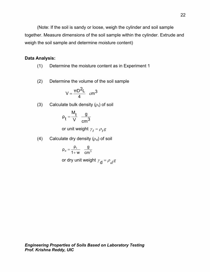
(Note: If the soil is sandy or loose, weigh the cylinder and soil sample
together. Measure dimensions of the soil sample within the cylinder. Extrude and
weigh the soil sample and determine moisture content)
Data Analysis:
(1) Determine the moisture content as in Experiment 1
(2) Determine the volume of the soil sample
3m4
L2πDV c=
(3) Calculate bulk density (ρt) of soil
3cmg
VtM
tρ =
or unit weight gtt ργ =
(4) Calculate dry density (ρd) of soil
3t
d cmg
w1ρ
ρ+
=
or dry unit weight gdργ =d

Engineering Properties of Soils Based on Laboratory Testing Prof. Krishna Reddy, UIC
23
EXAMPLE DATA

Engineering Properties of Soils Based on Laboratory Testing Prof. Krishna Reddy, UIC
24
DENSITY (UNIT WEIGHT) DETERMINATION DATA SHEET
Sample number: B-1, ST-1, 10’-12’ Date Tested: September 10, 2002
Soil description: Gray silty clay
Mass of the soil sample (Mt): 125.20 grams
Length of the soil sample (L): 7.26 cm
Diameter of the soil sample (D): 3.41 cm
Moisture content determination: Specimen number 1
Moisture can and lid number 15
MC = Mass of empty, clean can + lid (grams) 7.83
MCMS = Mass of can, lid, and moist soil (grams) 13.43
MCDS = Mass of can, lid, and dry soil (grams) 12.69
MS = Mass of soil solids (grams) 4.86
MW = Mass of pore water (grams) 0.74
w = Water content, w% 15. 2
Example calculations: w=15.2%, Mt=125.2g, L=7.26cm, D=3.41cm
( ) ( ) 3cm66.28
4
7.2623.41πV ==
3ft
Ib11862.4 1.89tor3cm
g1.89
66.28125.20
t =×=== γρ
3ft
Ib102.362.41.64dor
3cm
g1.64
100
15.201
1.89d =×==
+=
γρ
(Note: 62.4 is the conversion factor to convert density in g/cm3 to unit weight in
lb/ft3)

Engineering Properties of Soils Based on Laboratory Testing Prof. Krishna Reddy, UIC
25
BLANK DATA SHEETS

Engineering Properties of Soils Based on Laboratory Testing Prof. Krishna Reddy, UIC
26
DENSITY (UNIT WEIGHT) DETERMINATION DATA SHEET
Sample number: Date Tested: Soil description: Mass of the soil sample (Mt): Length of the soil sample (L): Diameter of the soil sample (D): Moisture content determination:
Specimen number 1 Moisture can and lid number
MC = Mass of empty, clean can + lid (grams)
MCMS = Mass of can, lid, and moist soil (grams)
MCDS = Mass of can, lid, and dry soil (grams)
MS = Mass of soil solids (grams)
MW = Mass of pore water (grams)
w = Water content, w%
Calculations:

Engineering Properties of Soils Based on Laboratory Testing Prof. Krishna Reddy, UIC
27
EXPERIMENT 4 SPECIFIC GRAVITY DETERMINATION
Purpose: This lab is performed to determine the specific gravity of soil by
using a pycnometer. Specific gravity is the ratio of the mass of unit volume
of soil at a stated temperature to the mass of the same volume of gas-free
distilled water at a stated temperature.
Standard Reference: ASTM D 854-00 – Standard Test for Specific Gravity of Soil Solids
by Water Pycnometer.
Significance: The specific gravity of a soil is used in the phase relationship of air,
water, and solids in a given volume of the soil.
Equipment: Pycnometer, Balance, Vacuum pump, Funnel, Spoon.

Engineering Properties of Soils Based on Laboratory Testing Prof. Krishna Reddy, UIC
28
Test Procedure:
(1) Determine and record the weight of the empty clean and dry
pycnometer, WP.
(2) Place 10g of a dry soil sample (passed through the sieve No. 10)
in the pycnometer. Determine and record the weight of the
pycnometer containing the dry soil, WPS.
(3) Add distilled water to fill about half to three-fourth of the
pycnometer. Soak the sample for 10 minutes.
(4) Apply a partial vacuum to the contents for 10 minutes, to remove
the entrapped air.

Engineering Properties of Soils Based on Laboratory Testing Prof. Krishna Reddy, UIC
29
(5) Stop the vacuum and carefully remove the vacuum line from
pycnometer.
(6) Fill the pycnometer with distilled (water to the mark), clean the
exterior surface of the pycnometer with a clean, dry cloth.
Determine the weight of the pycnometer and contents, WB.
(7) Empty the pycnometer and clean it. Then fill it with distilled water
only (to the mark). Clean the exterior surface of the pycnometer
with a clean, dry cloth. Determine the weight of the pycnometer
and distilled water, WA.
(8) Empty the pycnometer and clean it.
Data Analysis: Calculate the specific gravity of the soil solids using the following
formula:
)W(WWWGGravity,Specific
BA0
0S −+=
Where:
W0 = weight of sample of oven-dry soil, g = WPS - WP
WA = weight of pycnometer filled with water
WB = weight of pycnometer filled with water and soil
Engineering Properties of Soils Based on Laboratory Testing Prof. Krishna Reddy, UIC
30
EXAMPLE DATA
Engineering Properties of Soils Based on Laboratory Testing Prof. Krishna Reddy, UIC
31
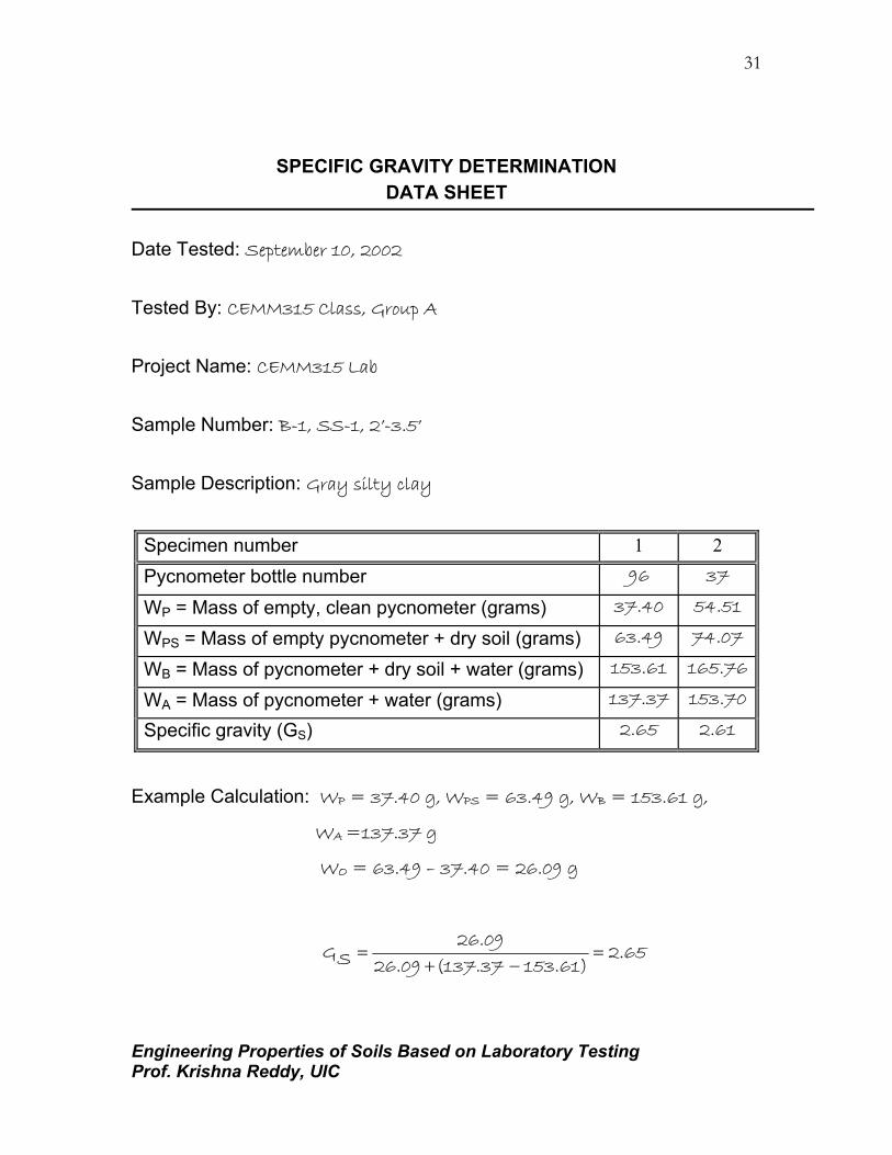
SPECIFIC GRAVITY DETERMINATION DATA SHEET
Date Tested: September 10, 2002 Tested By: CEMM315 Class, Group A
Project Name: CEMM315 Lab
Sample Number: B-1, SS-1, 2’-3.5’
Sample Description: Gray silty clay
Specimen number 1 2
Pycnometer bottle number 96 37
WP = Mass of empty, clean pycnometer (grams) 37.40 54.51
WPS = Mass of empty pycnometer + dry soil (grams) 63.49 74.07
WB = Mass of pycnometer + dry soil + water (grams) 153.61 165.76
WA = Mass of pycnometer + water (grams) 137.37 153.70
Specific gravity (GS) 2.65 2.61
Example Calculation: WP = 37.40 g, WPS = 63.49 g, WB = 153.61 g,
WA =137.37 g
WO = 63.49 – 37.40 = 26.09 g
2.65153.61)(137.3726.09
26.09SG =
−+=

Engineering Properties of Soils Based on Laboratory Testing Prof. Krishna Reddy, UIC
32
BLANK DATA SHEETS
Engineering Properties of Soils Based on Laboratory Testing Prof. Krishna Reddy, UIC
33
SPECIFIC GRAVITY DETERMINATION DATA SHEET
Date Tested: Tested By: Project Name: Sample Number: Sample Description:
Specimen number 1 2
Pycnometer bottle number
WP = Mass of empty, clean pycnometer (grams)
WPS = Mass of empty pycnometer + dry soil (grams)
WB = Mass of pycnometer + dry soil + water (grams)
WA = Mass of pycnometer + water (grams)
Specific Gravity (GS)
Calculations:

Engineering Properties of Soils Based on Laboratory Testing Prof. Krishna Reddy, UIC
34
EXPERIMENT 5 RELATIVE DENSITY DETERMINATION
Purpose: This lab is performed to determine the relative density of cohesionless,
free-draining soils using a vibrating table. The relative density of a soil is the
ratio, expressed as a percentage, of the difference between the maximum index
void ratio and the field void ratio of a cohesionless, free-draining soil; to the
difference between its maximum and minimum index void ratios.
Standard References: ASTM D 4254 – Standard Test Methods for Minimum Index Density and
Unit Weight of Soils and Calculation of Relative Density.
ASTM D 4253 – Standard Test Methods for Maximum Index Density and
Unit Weight of Soils Using a Vibratory Table.
Significance: Relative density and percent compaction are commonly used for
evaluating the state of compactness of a given soil mass. The engineering
properties, such as shear strength, compressibility, and permeability, of a given
soil depend on the level of compaction. Equipment:
Vibrating Table, Mold Assembly consisting of standard mold, guide
sleeves, surcharge base-plate, surcharge weights, surcharge base-plate handle,
and dial-indicator gage, Balance, Scoop, Straightedge.

Engineering Properties of Soils Based on Laboratory Testing Prof. Krishna Reddy, UIC
35

Engineering Properties of Soils Based on Laboratory Testing Prof. Krishna Reddy, UIC
36
Test Procedure: (1) Fill the mold with the soil (approximately 0.5 inch to 1 inch above the
top of the mold) as loosely as possible by pouring the soil using a scoop
or pouring device (funnel). Spiraling motion should be just sufficient to
minimize particle segregation.
(2) Trim off the excess soil level with the top by carefully trimming the soil
surface with a straightedge.
(3) Determine and record the mass of the mold and soil. Then empty the
mold (M1). See Photograph on Page 35.
(4) Again fill the mold with soil (do not use the same soil used in step 1)
and level the surface of the soil by using a scoop or pouring device
(funnel) in order to minimize the soil segregation. The sides of the mold
may be struck a few times using a metal bar or rubber hammer to settle
the soil so that the surcharge base-plate can be easily placed into
position and there is no surge of air from the mold when vibration is
initiated.
(5) Place the surcharge base plate on the surface of the soil and twist it
slightly several times so that it is placed firmly and uniformly in contact
with the surface of the soil. Remove the surcharge base-plate handle.
(6) Attach the mold to the vibrating table.
(7) Determine the initial dial reading by inserting the dial indicator gauge
holder in each of the guide brackets with the dial gage stem in contact

Engineering Properties of Soils Based on Laboratory Testing Prof. Krishna Reddy, UIC
37
with the rim of the mold (at its center) on the both sides of the guide
brackets. Obtain six sets of dial indicator readings, three on each side
of each guide bracket. The average of these twelve readings is the
initial dial gage reading, Ri. Record Ri to the nearest 0.001 in. (0.025
mm). See Photograph on Page 35.
(8) Firmly attach the guide sleeve to the mold and lower the appropriate
surcharge weight onto the surcharge base-plate. See Photograph on
Page 35.
(9) Vibrate the mold assembly and soil specimen for 8 min.
(10) Determine and record the dial indicator gage readings as in step (7).
The average of these readings is the final dial gage reading, Rf.
(11) Remove the surcharge base-plate from the mold and detach the mold
from the vibrating table.
(12) Determine and record the mass of the mold and soil (M2)
(13) Empty the mold and determine the weight of the mold.
(14) Determine and record the dimensions of the mold (i.e., diameter and
height) in order to calculate the calibrated volume of the mold, Vc. Also,
determine the thickness of the surcharge base-plate, Tp.

Engineering Properties of Soils Based on Laboratory Testing Prof. Krishna Reddy, UIC
38
Analysis:
(1) Calculate the minimum index density (ρdmin) as follows:
CVS1M
dminρ =
where
Ms1= mass of tested-dry soil
= Mass of mold with soil placed loose – mass of mold
Vc= Calibrated volume of the mold
(2) Calculate the maximum index density (ρdmax) as follows:
VS2M
dmaxρ =
where
Ms2 = mass of tested-dry soil
= Mass of mold with soil after vibration – Mass of mold
V = Volume of tested-dry soil
= Vc – (Ac*H)
Where
Ac = the calibrated cross sectional area of the mold
H = Rf -Ri+ Tp

Engineering Properties of Soils Based on Laboratory Testing Prof. Krishna Reddy, UIC
39
(3) Calculate the maximum and the minimum-index void ratios as follows (use
Gs value determined from Experiment 4; ρw=1 g/cm3):
1dmin
ρsGwρ
mine −=
1dmin
ρsGwρ
maxe −=
(4) Calculate the relative density as follows:
minemaxeemaxe
dD−−
=
[Calculate the void ratio of the natural state of the soil based on ρd (Experiment 3)
and ρs=GS*ρw (Gs determined from Experiment 4) as follows: 1dρsρe −= ]

Engineering Properties of Soils Based on Laboratory Testing Prof. Krishna Reddy, UIC
40
EXAMPLE DATA `

Engineering Properties of Soils Based on Laboratory Testing Prof. Krishna Reddy, UIC
41
RELATIVE DENSITY DETERMINATION DATA SHEET
Date Tested: September 10, 2002 Tested By: CEMM315 Class, Group A
Project Name: CEMM315 Lab
Sample Number: B-1, ST-1, 2’-3.5’
Sample Description: Brown sand Mass of empty mold: __9.878 Kg _ Diameter of empty mold: __15.45 cm____ Height of empty mold: __15.50 cm____ Mass of mold and soil (M1): __14.29 Kg_ Average initial dial gauge reading (Ri): __0.88 inches__ Average final dial gauge reading (Rf): __0.40 inches__ Thickness of surcharge base plate (TP): __0.123 inches_ Mass of mold and soil (M2): __14.38 Kg__ Calculations:
( )
( )
65%1000.540.74
0.610.74D
0.7411.52
2.651e,0.541
1.72
2.651e
cm
g1.72
2618.75
4502,
cm
g1.52
2905.88
4412
cm2618.751.53187.472905.88V,cm2905.884
15.5(15.45)V
cm1.532.540.123)0.4(0.88H,cm187.474
15.45A
g4502kg4.5029.87814.38M,g4412kg4.4129.87814.29M
d
maxmin
3dmax3dmin
332
C
22
C
S2S1
0.611-1.65
2.65e
soil)thisusingconducted3Experimenton(Based3cm
g1.65d
soil)theusingconducted4Experimenton2.65(BasedGs
=−−
=
=−×
==−×
=
====
=×−===
=×+−===
==−===−=
==
−=
−=
x
ρ
ρρ
π
π

Engineering Properties of Soils Based on Laboratory Testing Prof. Krishna Reddy, UIC
42
BLANK DATA SHEETS

Engineering Properties of Soils Based on Laboratory Testing Prof. Krishna Reddy, UIC
43
RELATIVE DENSITY DETERMINATION DATA SHEET
Date Tested: Tested By: Project Name: Sample Number: Sample Description: Mass of empty mold: __ ______________ Diameter of empty mold: __ ______________ Height of empty mold: __ ______________ Mass of mold and soil (M1): __ ______________ Average initial dial gauge reading (Ri): __ ______________ Average final dial gauge reading (Rf): __ ______________ Thickness of surcharge base plate (TP): __ ______________ Mass of mold and soil (M2): __ ______________ Calculations:

Engineering Properties of Soils Based on Laboratory Testing Prof. Krishna Reddy, UIC
44
EXPERIMENT 6 GRAIN SIZE ANALYSIS
(SIEVE AND HYDROMETER ANALYSIS)
Purpose:
This test is performed to determine the percentage of different grain sizes
contained within a soil. The mechanical or sieve analysis is performed to
determine the distribution of the coarser, larger-sized particles, and the hydrometer
method is used to determine the distribution of the finer particles.
Standard Reference:
ASTM D 422 - Standard Test Method for Particle-Size Analysis of Soils
Significance:
The distribution of different grain sizes affects the engineering properties of
soil. Grain size analysis provides the grain size distribution, and it is required in
classifying the soil.
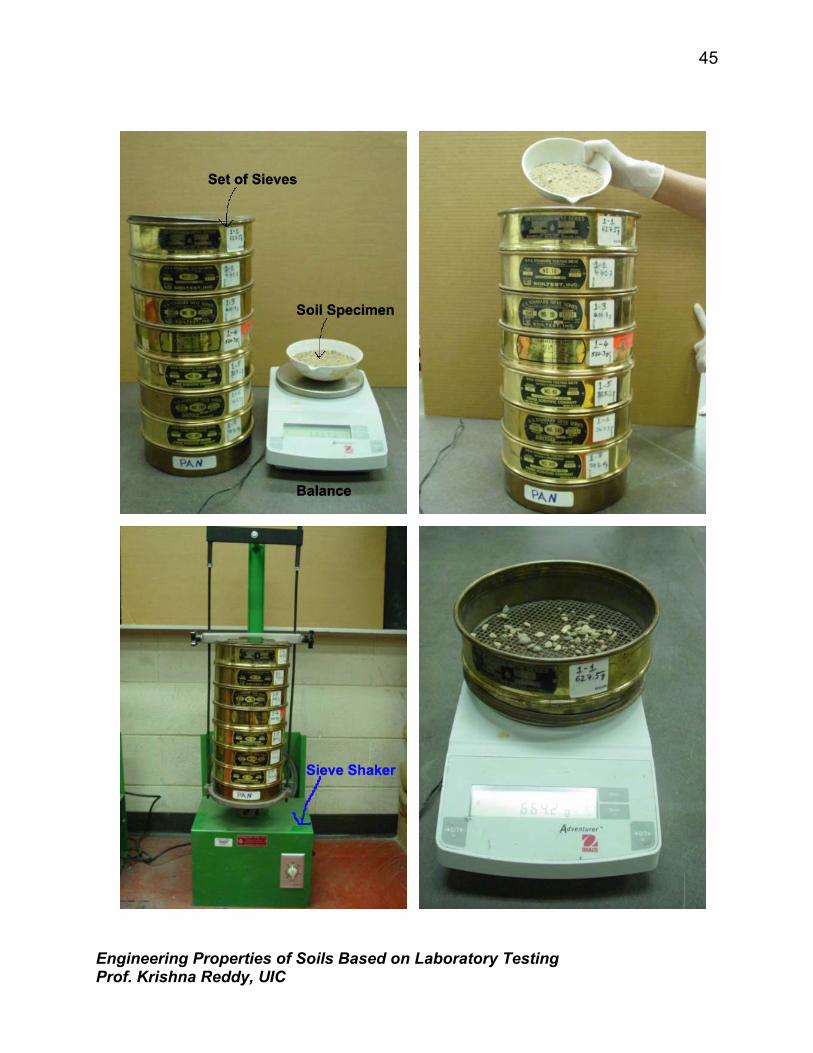
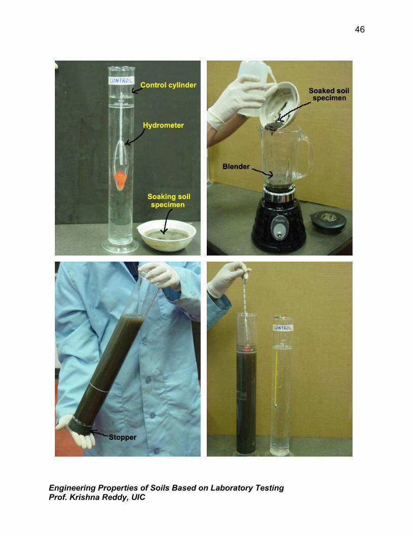
Equipment: Balance, Set of sieves, Cleaning brush, Sieve shaker, Mixer (blender), 152H
Hydrometer, Sedimentation cylinder, Control cylinder, Thermometer, Beaker,
Timing device.
Engineering Properties of Soils Based on Laboratory Testing Prof. Krishna Reddy, UIC
45
Engineering Properties of Soils Based on Laboratory Testing Prof. Krishna Reddy, UIC
46
Engineering Properties of Soils Based on Laboratory Testing Prof. Krishna Reddy, UIC
47
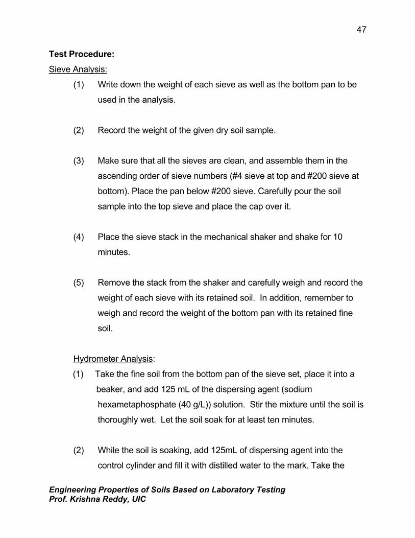
Test Procedure:
Sieve Analysis:
(1) Write down the weight of each sieve as well as the bottom pan to be
used in the analysis.
(2) Record the weight of the given dry soil sample.
(3) Make sure that all the sieves are clean, and assemble them in the
ascending order of sieve numbers (#4 sieve at top and #200 sieve at
bottom). Place the pan below #200 sieve. Carefully pour the soil
sample into the top sieve and place the cap over it.
(4) Place the sieve stack in the mechanical shaker and shake for 10
minutes.
(5) Remove the stack from the shaker and carefully weigh and record the
weight of each sieve with its retained soil. In addition, remember to
weigh and record the weight of the bottom pan with its retained fine
soil.
Hydrometer Analysis:
(1) Take the fine soil from the bottom pan of the sieve set, place it into a
beaker, and add 125 mL of the dispersing agent (sodium
hexametaphosphate (40 g/L)) solution. Stir the mixture until the soil is
thoroughly wet. Let the soil soak for at least ten minutes.
(2) While the soil is soaking, add 125mL of dispersing agent into the
control cylinder and fill it with distilled water to the mark. Take the
Engineering Properties of Soils Based on Laboratory Testing Prof. Krishna Reddy, UIC
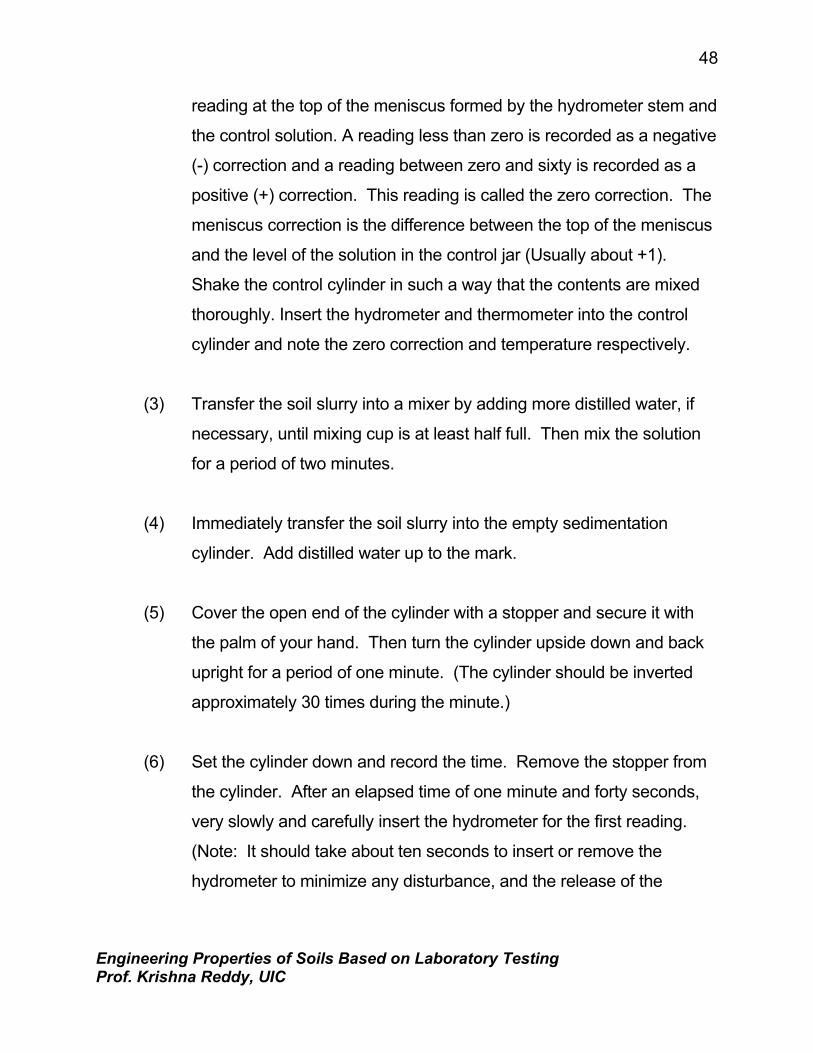
48
reading at the top of the meniscus formed by the hydrometer stem and
the control solution. A reading less than zero is recorded as a negative
(-) correction and a reading between zero and sixty is recorded as a
positive (+) correction. This reading is called the zero correction. The
meniscus correction is the difference between the top of the meniscus
and the level of the solution in the control jar (Usually about +1).
Shake the control cylinder in such a way that the contents are mixed
thoroughly. Insert the hydrometer and thermometer into the control
cylinder and note the zero correction and temperature respectively.
(3) Transfer the soil slurry into a mixer by adding more distilled water, if
necessary, until mixing cup is at least half full. Then mix the solution
for a period of two minutes.
(4) Immediately transfer the soil slurry into the empty sedimentation
cylinder. Add distilled water up to the mark.
(5) Cover the open end of the cylinder with a stopper and secure it with
the palm of your hand. Then turn the cylinder upside down and back
upright for a period of one minute. (The cylinder should be inverted
approximately 30 times during the minute.)
(6) Set the cylinder down and record the time. Remove the stopper from
the cylinder. After an elapsed time of one minute and forty seconds,
very slowly and carefully insert the hydrometer for the first reading.
(Note: It should take about ten seconds to insert or remove the
hydrometer to minimize any disturbance, and the release of the

Engineering Properties of Soils Based on Laboratory Testing Prof. Krishna Reddy, UIC
49
hydrometer should be made as close to the reading depth as possible
to avoid excessive bobbing).
(7) The reading is taken by observing the top of the meniscus formed by
the suspension and the hydrometer stem. The hydrometer is removed
slowly and placed back into the control cylinder. Very gently spin it in
control cylinder to remove any particles that may have adhered.
(8) Take hydrometer readings after elapsed time of 2 and 5, 8, 15, 30, 60
minutes and 24 hours
Data Analysis:
Sieve Analysis:
(1) Obtain the mass of soil retained on each sieve by subtracting the
weight of the empty sieve from the mass of the sieve + retained soil,
and record this mass as the weight retained on the data sheet. The
sum of these retained masses should be approximately equals the
initial mass of the soil sample. A loss of more than two percent is
unsatisfactory.
(2) Calculate the percent retained on each sieve by dividing the weight
retained on each sieve by the original sample mass.
(3) Calculate the percent passing (or percent finer) by starting with 100
percent and subtracting the percent retained on each sieve as a
cumulative procedure.
For example: Total mass = 500 g
Mass retained on No. 4 sieve = 9.7 g

Engineering Properties of Soils Based on Laboratory Testing Prof. Krishna Reddy, UIC
50
Mass retained on No. 10 sieve = 39.5 g
For the No.4 sieve:
Quantity passing = Total mass - Mass retained
= 500 - 9.7 = 490.3 g
The percent retained is calculated as;
% retained = Mass retained/Total mass
= (9.7/500) X 100 = 1.9 %
From this, the % passing = 100 - 1.9 = 98.1 %
For the No. 10 sieve:
Quantity passing = Mass arriving - Mass retained
= 490.3 - 39.5 = 450.8 g
% Retained = (39.5/500) X 100 = 7.9 %
% Passing = 100 - 1.9 - 7.9 = 90.2 %
(Alternatively, use % passing = % Arriving - % Retained
For No. 10 sieve = 98.1 - 7.9 = 90.2 %)
(4) Make a semilogarithmic plot of grain size vs. percent finer.
(5) Compute Cc and Cu for the soil.
Hydrometer Analysis:
(1) Apply meniscus correction to the actual hydrometer reading.
(2) From Table 1, obtain the effective hydrometer depth L in cm (for
meniscus corrected reading).

Engineering Properties of Soils Based on Laboratory Testing Prof. Krishna Reddy, UIC
51
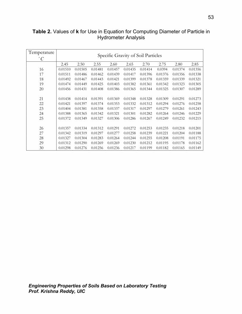
(3) For known Gs of the soil (if not known, assume 2.65 for this lab
purpose), obtain the value of K from Table 2.
(4) Calculate the equivalent particle diameter by using the following
formula:
tLKD =
Where t is in minutes, and D is given in mm.
(5) Determine the temperature correction CT from Table 3.
(6) Determine correction factor “a” from Table 4 using Gs.
(7) Calculate corrected hydrometer reading as follows:
Rc = RACTUAL - zero correction + CT
(8) Calculate percent finer as follows:
100sw
aRcP ××=
Where WS is the weight of the soil sample in grams.
(9) Adjusted percent fines as follows:
100200FP
AP×
=
F200 = % finer of #200 sieve as a percent
(10) Plot the grain size curve D versus the adjusted percent finer on the
semilogarithmic sheet.

Engineering Properties of Soils Based on Laboratory Testing Prof. Krishna Reddy, UIC
52
Table 1. Values of Effective Depth Based on Hydrometer and Sedimentation Cylinder of Specific Sizes
Hydrometer 151H Hydrometer 152H
Actual Hydrometer
Reading
Effective Depth, L (cm)
Actual Hydrometer
Reading
Effective Depth, L (cm)
Actual Hydrometer
Reading
Effective Depth, L (cm)
1.000 16.3 0 16.3 31 11.2 1.001 16.0 1 16.1 32 11.1 1.002 15.8 2 16.0 33 10.9 1.003 15.5 3 15.8 34 10.7 1.004 15.2 4 15.6 35 10.6 1.005 15.0 5 15.5 36 10.4 1.006 14.7 6 15.3 37 10.2 1.007 14.4 7 15.2 38 10.1 1.008 14.2 8 15.0 39 9.9 1.009 13.9 9 14.8 40 9.7 1.010 13.7 10 14.7 41 9.6 1.011 13.4 11 14.5 42 9.4 1.012 13.1 12 14.3 43 9.2 1.013 12.9 13 14.2 44 9.1 1.014 12.6 14 14.0 45 8.9 1.015 12.3 15 13.8 46 8.8 1.016 12.1 16 13.7 47 8.6 1.017 11.8 17 13.5 48 8.4 1.018 11.5 18 13.3 49 8.3 1.019 11.3 19 13.2 50 8.1 1.020 11.0 20 13.0 51 7.9 1.021 10.7 21 12.9 52 7.8 1.022 10.5 22 12.7 53 7.6 1.023 10.2 23 12.5 54 7.4 1.024 10.0 24 12.4 55 7.3 1.025 9.7 25 12.2 56 7.1 1.026 9.4 26 12.0 57 7.0 1.027 9.2 27 11.9 58 6.8 1.028 8.9 28 11.7 59 6.6 1.029 8.6 29 11.5 60 6.5 1.030 8.4 30 11.4 1.031 8.1 1.032 7.8 1.033 7.6 1.034 7.3 1.035 7.0 1.036 6.8 1.037 6.5 1.038 6.2 1.039 5.9
Engineering Properties of Soils Based on Laboratory Testing Prof. Krishna Reddy, UIC
53
Table 2. Values of k for Use in Equation for Computing Diameter of Particle in Hydrometer Analysis
Temperature Co
Specific Gravity of Soil Particles
2.45 2.50 2.55 2.60 2.65 2.70 2.75 2.80 2.85 16 0.01510 0.01505 0.01481 0.01457 0.01435 0.01414 0.0394 0.01374 0.0135617 0.01511 0.01486 0.01462 0.01439 0.01417 0.01396 0.01376 0.01356 0.0133818 0.01492 0.01467 0.01443 0.01421 0.01399 0.01378 0.01359 0.01339 0.0132119 0.01474 0.01449 0.01425 0.01403 0.01382 0.01361 0.01342 0.01323 0.0130520 0.01456 0.01431 0.01408 0.01386 0.01365 0.01344 0.01325 0.01307 0.01289
21 0.01438 0.01414 0.01391 0.01369 0.01348 0.01328 0.01309 0.01291 0.0127322 0.01421 0.01397 0.01374 0.01353 0.01332 0.01312 0.01294 0.01276 0.0125823 0.01404 0.01381 0.01358 0.01337 0.01317 0.01297 0.01279 0.01261 0.0124324 0.01388 0.01365 0.01342 0.01321 0.01301 0.01282 0.01264 0.01246 0.0122925 0.01372 0.01349 0.01327 0.01306 0.01286 0.01267 0.01249 0.01232 0.01215
26 0.01357 0.01334 0.01312 0.01291 0.01272 0.01253 0.01235 0.01218 0.0120127 0.01342 0.01319 0.01297 0.01277 0.01258 0.01239 0.01221 0.01204 0.0118828 0.01327 0.01304 0.01283 0.01264 0.01244 0.01255 0.01208 0.01191 0.0117529 0.01312 0.01290 0.01269 0.01269 0.01230 0.01212 0.01195 0.01178 0.0116230 0.01298 0.01276 0.01256 0.01236 0.01217 0.01199 0.01182 0.01165 0.01149

Engineering Properties of Soils Based on Laboratory Testing Prof. Krishna Reddy, UIC
54
Table 3. Temperature Correction Factors CT
Temperature Co
factor CT
15 1.10 16 -0.90 17 -0.70 18 -0.50 19 -0.30 20 0.00 21 +0.20 22 +0.40 23 +0.70 24 +1.00 25 +1.30 26 +1.65 27 +2.00 28 +2.50 29 +3.05 30 +3.80
Table 4. Correction Factors a for Unit Weight of Solids
Unit Weight of Soil Solids,
g/cm3
Correction factor
a 2.85 0.96 2.80 0.97 2.75 0.98 2.70 0.99 2.65 1.00 2.60 1.01 2.55 1.02 2.50 1.04
Engineering Properties of Soils Based on Laboratory Testing Prof. Krishna Reddy, UIC
55
EXAMPLE DATA

Engineering Properties of Soils Based on Laboratory Testing Prof. Krishna Reddy, UIC
56
Grain Size Analysis
Sieve Analysis
Date Tested: September 15, 2002 Tested By: CEMM315 Class, Group A Project Name: CEMM315 Lab Sample Number: B-1, ST-1, 2’-3. 5’ Visual Classification of Soil: Brown Clayey to silty sand, trace fine gravel Weight of Container: 198.5 gm Wt. Container+Dry Soil: 722.3 gm Wt. of Dry Sample: 523.8 gm
Sieve Number
Diameter (mm)
Mass of Empty
Sieve (g)
Mass of Sieve+Soil
Retained (g)
Soil Retained
(g)
Percent Retained
Percent Passing
4 4.75 116.23 166.13 49.9 9.5 90.5
10 2. 0 99.27 135.77 36.5 7.0 83.5
20 0.84 97.58 139.68 42.1 8.0 75.5
40 0.425 98.96 138.96 40.0 7.6 67.8
60 0. 25 91.46 114.46 23.0 4.4 63.4
140 0.106 93.15 184.15 91.0 17.4 46.1
200 0.075 90.92 101.12 10.2 1.9 44.1
Pan --- 70.19 301.19 231.0 44.1 0.0
Total Weight= 523.7
* Percent passing=100-cumulative percent retained. From Grain Size Distribution Curve: % Gravel= 9.5_ D10= 0.002____ mm % Sand= 46.4_ D30= 0.017___ mm % Fines= 44.1_ D60= .0.25 __ mm
( )0.58
0.0020.25
20.017cC125,
0.002
0.25uC =
×===
Unified Classification of Soil: SC/SM_

Engineering Properties of Soils Based on Laboratory Testing Prof. Krishna Reddy, UIC
57
Hydrometer Analysis
Test Date: September 15, 2002 Tested By: CEMM315 Class, Group A Hydrometer Number (if known): 152 H Specific Gravity of Solids: 2.56 Dispersing Agent: Sodium Hexametaphosphate Weight of Soil Sample: 50. 0 gm Zero Correction: +6 Meniscus Correction: +1
Date Time Elapsed Time (min)
Temp. OC
Actual Hydro. Rdg. Ra
Hyd. Corr. for Meniscus
L from Table 1
K from Table 2
D mm
CT from Table 3
a from Table 4
Corr. Hydr. Rdg. Rc
% Finer P
% Adjusted Finer PA
09/15 4:06 PM 0 25 55 56 7.1 0.01326 0 +1.3 1. 018 - - -
4:07 1 25 47 48 8.6 0.01326 0. 03029 +1.3 1. 018 42.3 86.1 37.8
4:08 2 25 42 43 9.2 0.01326 0.02844 +1.3 1. 018 37.3 75.9 33.3
4:10 4 25 40 41 9.6 0.01326 0.02054 +1.3 1. 018 35.3 71.9 31.6
4:14 8 25 37 38 10.1 0.01326 0.01490 +1.3 1. 018 32.3 65.8 28.6
4:22 16 25 32 33 10.9 0.01326 0.01094 +1.3 1. 018 27.3 55.6 24.1
4:40 34 25 28 29 11.5 0.01326 0.00771 +1.3 1. 018 23.3 47.4 20.8
6:22 136 23 22 23 12.5 0.01356 0.00411 +0.7 1. 018 16.7 34 14.9
09/16 5:24 PM 1518 22 15 16 13.7 0.01366 0.00130 +0.4 1. 018 9.4 19.1 8.4
Unified Classification of Soil: SC/SM

Engi
neer
ing
Prop
ertie
s of
Soi
ls B
ased
on
Labo
rato
ry T
estin
g Pr
of. K
rishn
a R
eddy
, UIC
58
GRA
IN S
IZE
ANAL
YSIS
0102030405060708090100
0.00
10.
010
0.10
01.
000
10.0
0010
0.00
010
00.0
00
GRAI
N SI
ZE -
mm
PERCENT FINER

Engineering Properties of Soils Based on Laboratory Testing Prof. Krishna Reddy, UIC
59
BLANK DATA SHEETS

Engineering Properties of Soils Based on Laboratory Testing Prof. Krishna Reddy, UIC
57
Grain Size Analysis
Sieve Analysis
Date Tested: Tested By: Project Name: Sample Number: Visual Classification of Soil: Weight of Container: _____gm Wt. Container+Dry Soil: _____gm Wt. of Dry Sample: _____gm
Sieve Number
Diameter (mm)
Mass of Empty
Sieve (g)
Mass of Sieve+Soil
Retained (g)
Soil Retained
(g)
Percent Retained
Percent Passing
4 4.75
10 2. 0
20 0.84
40 0.425
60 0. 25
140 0.106
200 0.075
Pan ---
Total Weight=
* Percent passing=100-cumulative percent retained.
From Grain Size Distribution Curve:
% Gravel= _______ D10= ________ mm
% Sand= _______ D30= ________ mm
% Fines= _______ D60= __ mm
Cu= ______________ CC= ________
Unified Classification of Soil: ________

Engineering Properties of Soils Based on Laboratory Testing Prof. Krishna Reddy, UIC
58
Hydrometer Analysis
Test Date: __________ Tested By: __________ Hydrometer Number (if known): _________ Specific Gravity of Solids: _________ Dispersing Agent: _________ Weight of Soil Sample: _________gm Zero Correction: _________ Meniscus Correction: _________
Date Time Elapsed Time (min)
Temp. OC
Actual Hydro. Rdg. Ra
Hyd. Corr. for Meniscus
L from Table 1
K from Table 2
D mm
CT from Table 3
a from Table 4
Corr. Hydr. Rdg. Rc
% Finer P
% Adjusted Finer PA
Unified Classification of Soil:

Engi
neer
ing
Prop
ertie
s of
Soi
ls B
ased
on
Labo
rato
ry T
estin
g Pr
of. K
rishn
a R
eddy
, UIC
59
Not
e: Y
ou c
an p
lot y
our d
ata
on th
is g
raph
or g
ener
ate
sim
ilar g
raph
usi
ng a
ny g
raph
ics
prog
ram
(e.g
., ex
cel)
0102030405060708090100
0.00
10.
010.
11
1010
010
00
Gra
in S
ize
(mm
)
Percent Passing

Engineering Properties of Soils Based on Laboratory Testing Prof. Krishna Reddy, UIC
60
EXPERIMENT 7 ATTERBERG LIMITS
Purpose:
This lab is performed to determine the plastic and liquid limits of a fine-
grained soil. The liquid limit (LL) is arbitrarily defined as the water content, in
percent, at which a pat of soil in a standard cup and cut by a groove of standard
dimensions will flow together at the base of the groove for a distance of 13 mm (1/2
in.) when subjected to 25 shocks from the cup being dropped 10 mm in a standard
liquid limit apparatus operated at a rate of two shocks per second. The plastic limit
(PL) is the water content, in percent, at which a soil can no longer be deformed by
rolling into 3.2 mm (1/8 in.) diameter threads without crumbling.
Standard Reference:
ASTM D 4318 - Standard Test Method for Liquid Limit, Plastic Limit, and
Plasticity Index of Soils
Significance:
The Swedish soil scientist Albert Atterberg originally defined seven “limits of
consistency” to classify fine-grained soils, but in current engineering practice only
two of the limits, the liquid and plastic limits, are commonly used. (A third limit,
called the shrinkage limit, is used occasionally.) The Atterberg limits are based on
the moisture content of the soil. The plastic limit is the moisture content that
defines where the soil changes from a semi-solid to a plastic (flexible) state. The
liquid limit is the moisture content that defines where the soil changes from a plastic
to a viscous fluid state. The shrinkage limit is the moisture content that defines
where the soil volume will not reduce further if the moisture content is reduced. A

Engineering Properties of Soils Based on Laboratory Testing Prof. Krishna Reddy, UIC
61
wide variety of soil engineering properties have been correlated to the liquid and
plastic limits, and these Atterberg limits are also used to classify a fine-grained soil
according to the Unified Soil Classification system or AASHTO system.
Equipment: Liquid limit device, Porcelain (evaporating) dish, Flat grooving tool with gage,
Eight moisture cans, Balance, Glass plate, Spatula, Wash bottle filled with distilled
water, Drying oven set at 105°C.

Engineering Properties of Soils Based on Laboratory Testing Prof. Krishna Reddy, UIC
62
Engineering Properties of Soils Based on Laboratory Testing Prof. Krishna Reddy, UIC
63
Test Procedure:
Liquid Limit:
(1) Take roughly 3/4 of the soil and place it into the porcelain dish.
Assume that the soil was previously passed though a No. 40 sieve,
air-dried, and then pulverized. Thoroughly mix the soil with a small
amount of distilled water until it appears as a smooth uniform paste.
Cover the dish with cellophane to prevent moisture from escaping.
(2) Weigh four of the empty moisture cans with their lids, and record the
respective weights and can numbers on the data sheet.
(3) Adjust the liquid limit apparatus by checking the height of drop of the
cup. The point on the cup that comes in contact with the base should
rise to a height of 10 mm. The block on the end of the grooving tool is

Engineering Properties of Soils Based on Laboratory Testing Prof. Krishna Reddy, UIC
64
10 mm high and should be used as a gage. Practice using the cup
and determine the correct rate to rotate the crank so that the cup
drops approximately two times per second.
(4) Place a portion of the previously mixed soil into the cup of the liquid
limit apparatus at the point where the cup rests on the base. Squeeze
the soil down to eliminate air pockets and spread it into the cup to a
depth of about 10 mm at its deepest point. The soil pat should form
an approximately horizontal surface (See Photo B).
(5) Use the grooving tool carefully cut a clean straight groove down the
center of the cup. The tool should remain perpendicular to the surface
of the cup as groove is being made. Use extreme care to prevent
sliding the soil relative to the surface of the cup (See Photo C).
(6) Make sure that the base of the apparatus below the cup and the
underside of the cup is clean of soil. Turn the crank of the apparatus
at a rate of approximately two drops per second and count the number
of drops, N, it takes to make the two halves of the soil pat come into
contact at the bottom of the groove along a distance of 13 mm (1/2 in.)
(See Photo D). If the number of drops exceeds 50, then go directly to
step eight and do not record the number of drops, otherwise, record
the number of drops on the data sheet.
(7) Take a sample, using the spatula, from edge to edge of the soil pat.
The sample should include the soil on both sides of where the groove
came into contact. Place the soil into a moisture can cover it.
Immediately weigh the moisture can containing the soil, record its

Engineering Properties of Soils Based on Laboratory Testing Prof. Krishna Reddy, UIC
65
mass, remove the lid, and place the can into the oven. Leave the
moisture can in the oven for at least 16 hours. Place the soil
remaining in the cup into the porcelain dish. Clean and dry the cup on
the apparatus and the grooving tool.
(8) Remix the entire soil specimen in the porcelain dish. Add a small
amount of distilled water to increase the water content so that the
number of drops required to close the groove decrease.
(9) Repeat steps six, seven, and eight for at least two additional trials
producing successively lower numbers of drops to close the groove.
One of the trials shall be for a closure requiring 25 to 35 drops, one for
closure between 20 and 30 drops, and one trial for a closure requiring
15 to 25 drops. Determine the water content from each trial by using
the same method used in the first laboratory. Remember to use the
same balance for all weighing.
Plastic Limit:
(1) Weigh the remaining empty moisture cans with their lids, and record
the respective weights and can numbers on the data sheet.
(2) Take the remaining 1/4 of the original soil sample and add distilled
water until the soil is at a consistency where it can be rolled without
sticking to the hands.
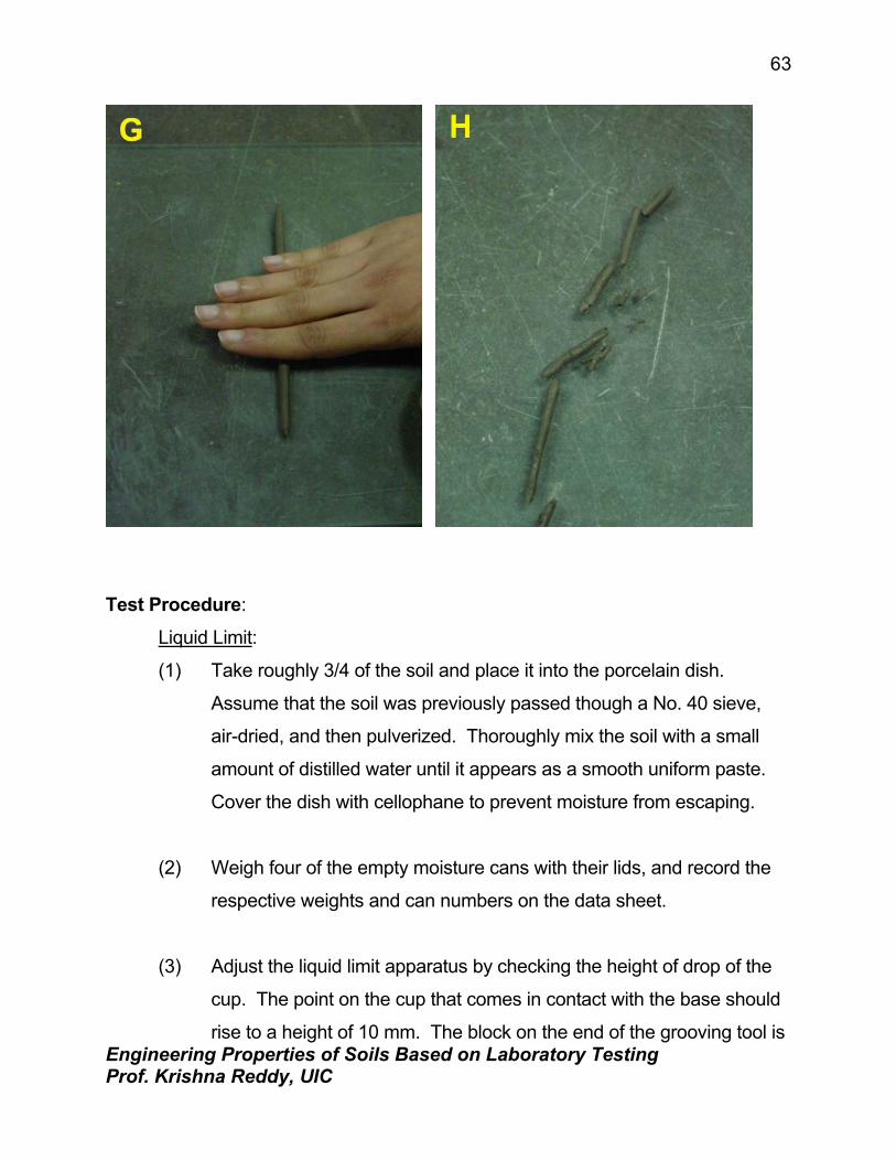
(3) Form the soil into an ellipsoidal mass (See Photo F). Roll the mass
between the palm or the fingers and the glass plate (See Photo G).
Use sufficient pressure to roll the mass into a thread of uniform

Engineering Properties of Soils Based on Laboratory Testing Prof. Krishna Reddy, UIC
66
diameter by using about 90 strokes per minute. (A stroke is one
complete motion of the hand forward and back to the starting position.)
The thread shall be deformed so that its diameter reaches 3.2 mm (1/8
in.), taking no more than two minutes.
(4) When the diameter of the thread reaches the correct diameter, break
the thread into several pieces. Knead and reform the pieces into
ellipsoidal masses and re-roll them. Continue this alternate rolling,
gathering together, kneading and re-rolling until the thread crumbles
under the pressure required for rolling and can no longer be rolled into
a 3.2 mm diameter thread (See Photo H).
(5) Gather the portions of the crumbled thread together and place the soil
into a moisture can, then cover it. If the can does not contain at least
6 grams of soil, add soil to the can from the next trial (See Step 6).
Immediately weigh the moisture can containing the soil, record its
mass, remove the lid, and place the can into the oven. Leave the
moisture can in the oven for at least 16 hours.
(6) Repeat steps three, four, and five at least two more times. Determine
the water content from each trial by using the same method used in
the first laboratory. Remember to use the same balance for all
weighing.

Engineering Properties of Soils Based on Laboratory Testing Prof. Krishna Reddy, UIC
67
Analysis:
Liquid Limit:
(1) Calculate the water content of each of the liquid limit moisture cans
after they have been in the oven for at least 16 hours.
(2) Plot the number of drops, N, (on the log scale) versus the water
content (w). Draw the best-fit straight line through the plotted points
and determine the liquid limit (LL) as the water content at 25 drops.
Plastic Limit:
(1) Calculate the water content of each of the plastic limit moisture cans
after they have been in the oven for at least 16 hours.
(2) Compute the average of the water contents to determine the plastic
limit, PL. Check to see if the difference between the water contents is
greater than the acceptable range of two results (2.6 %).
(3) Calculate the plasticity index, PI=LL-PL.
Report the liquid limit, plastic limit, and plasticity index to the nearest
whole number, omitting the percent designation.

Engineering Properties of Soils Based on Laboratory Testing Prof. Krishna Reddy, UIC
68
EXAMPLE DATA

Engineering Properties of Soils Based on Laboratory Testing Prof. Krishna Reddy, UIC
69
ATTERBERG LIMITS DATA SHEETS
Date Tested: September 20, 2002
Tested By: CEMM315 Class, Group A
Project Name: CEMM315 Lab
Sample Number: B-1, SS-1, 8’-10’
Sample Description: Grayey silty clay
Liquid Limit Determination
Sample no. 1 2 3 4 Moisture can and lid number 11 1 5 4
MC = Mass of empty, clean can + lid (grams) 22.23 23.31 21.87 22.58 MCMS = Mass of can, lid, and moist soil (grams) 28.56 29.27 25.73 25.22 MCDS = Mass of can, lid, and dry soil (grams) 27.40 28.10 24.90 24.60 MS = Mass of soil solids (grams) 5.03 4.79 3.03 2.02 MW = Mass of pore water (grams) 1.16 1.17 0.83 0.62 w = Water content, w% 23.06 24.43 27.39 30.69 No. of drops (N) 31 29 20 14
Plastic Limit Determination
Sample no. 1 2 3 Moisture can and lid number 7 14 13
MC = Mass of empty, clean can + lid (grams) 7.78 7.83 15.16
MCMS = Mass of can, lid, and moist soil (grams) 16.39 13.43 21.23
MCDS = Mass of can, lid, and dry soil (grams) 15.28 12 .69 20.43
MS = Mass of soil solids (grams) 7.5 4.86 5.27
MW = Mass of pore water (grams) 1. 11 0.74 0.8
w = Water content, w% 14.8 15.2 15.1
Plastic Limit (PL)= Average w % = 15.03
15.115.214.8 =++

Engineering Properties of Soils Based on Laboratory Testing Prof. Krishna Reddy, UIC
70
LIQUID LIMIT CHART
From the above graph, Liquid Limit = 26
Final Results: Liquid Limit = 26 Plastic Limit = 15 Plasticity Index =11
0
5
10
15
20
25
30
35
0 5 10 15 20 25 30 35
No. of Blows, N
Wat
er C
onte
nt, w
%
Engineering Properties of Soils Based on Laboratory Testing Prof. Krishna Reddy, UIC
71
BLANK DATA SHEETS

Engineering Properties of Soils Based on Laboratory Testing Prof. Krishna Reddy, UIC
72
ATTERBERG LIMITS DATA SHEETS
Date Tested: Tested By:
Project Name:
Sample Number:
Sample Description: Liquid Limit Determination
Sample no. 1 2 3 4 Moisture can and lid number
MC = Mass of empty, clean can + lid (grams)
MCMS = Mass of can, lid, and moist soil (grams)
MCDS = Mass of can, lid, and dry soil (grams)
MS = Mass of soil solids (grams)
MW = Mass of pore water (grams)
w = Water content, w%
No. of drops (N)
Plastic Limit Determination
Sample no. 1 2 3 Moisture can and lid number
MC = Mass of empty, clean can + lid (grams)
MCMS = Mass of can, lid, and moist soil (grams)
MCDS = Mass of can, lid, and dry soil (grams)
MS = Mass of soil solids (grams)
MW = Mass of pore water (grams)
w = Water content, w%
Plastic Limit (PL) = Average w % =

Engineering Properties of Soils Based on Laboratory Testing Prof. Krishna Reddy, UIC
73
LIQUID LIMIT CHART
0
5
10
15
20
25
30
35
40
0 10 20 30 40 50
No. of Blows, N
Wat
er C
onte
nt, w
%
Final Results: Liquid Limit = Plastic Limit = Plasticity Index =
Engineering Properties of Soils Based on Laboratory Testing Prof. Krishna Reddy, UIC
74
EXPERIMENT 7 VISUAL CLASSIFICATION OF SOILS
Purpose:
Visually classify the soils.
Standard Reference:
ASTM D 2488 - Standard Practice for Description and Identification of
Soils (Visual - Manual Procedure)
Significance: The first step in any geotechnical engineering project is to identify and
describe the subsoil condition. For example, as soon as a ground is
identified as gravel, engineer can immediately form some ideas on the
nature of problems that might be encountered in a tunneling project. In
contrast, a soft clay ground is expected to lead to other types of design and
construction considerations. Therefore, it is useful to have a systematic
procedure for identification of soils even in the planning stages of a project.
Soils can be classified into two general categories: (1) coarse grained
soils and (2) fine grained soils. Examples of coarse-grained soils are gravels
and sands. Examples of fine-grained soils are silts and clays. Procedures
for visually identifying these two general types of soils are described in the
following sections.
Equipment: Magnifying glass (optional)

Engineering Properties of Soils Based on Laboratory Testing Prof. Krishna Reddy, UIC
75
Identification Procedure: a. Identify the color (e.g. brown, gray, brownish gray), odor (if any)
and texture (coarse or fine-grained) of soil.
b. Identify the major soil constituent (>50% by weight) using Table
1 as coarse gravel, fine gravel, coarse sand, medium sand, fine
sand, or fines.
c. Estimate percentages of all other soil constituents using Table 1
and the following terms:
Trace - 0 to 10% by weight
Little - 10 to 20%
Some - 20 to 30%
And - 30 to 50%
(Examples: trace fine gravel, little silt, some clay)
d. If the major soil constituent is sand or gravel:
Identify particle distribution. Describe as well graded or poorly graded. Well-graded soil consists of particle sizes over a wide
range. Poorly graded soil consists of particles which are all
about the same size.
Identify particle shape (angular, subangular, rounded,
subrounded) using Figure 1 and Table 2.

Engineering Properties of Soils Based on Laboratory Testing Prof. Krishna Reddy, UIC
76
e. If the major soil constituents are fines, perform the following
tests:
Dry strength test: Mold a sample into 1/8" size ball and let it dry.
Test the strength of the dry sample by crushing it between the
fingers. Describe the strength as none, low, medium, high or
very high depending on the results of the test as shown in Table
3(a).
Dilatancy Test: Make a sample of soft putty consistency in your
palm. Then observe the reaction during shaking, squeezing (by
closing hand) and vigorous tapping. The reaction is rapid, slow
or none according to the test results given in Table 3(b).
During dilatancy test, vibration densifies the silt and water
appears on the surface. Now on squeezing, shear stresses are
applied on the densified silt. The dense silt has a tendency for
volume increase or dilatancy due to shear stresses. So the
water disappears from the surface. Moreover, silty soil has a
high permeability, so the water moves quickly. In clay, we see
no change, no shiny surface, in other words, no reaction.
Plasticity (or Toughness) Test: Roll the samples into a thread
about 1/8" in diameter. Fold the thread and reroll it repeatedly
until the thread crumbles at a diameter of 1/8". Note (a) the
pressure required to roll the thread when it is near crumbling, (b)
whether it can support its own weight, (c) whether it can be
molded back into a coherent mass, and (d) whether it is tough

Engineering Properties of Soils Based on Laboratory Testing Prof. Krishna Reddy, UIC
77
during kneading. Describe the plasticity and toughness
according to the criteria in Tables 3(c) and 3(d). A low to
medium toughness and non-plastic to low plasticity is the
indication that the soil is silty; otherwise the soil is clayey.
Based on dry strength, dilatancy and toughness, determine soil
symbol based on Table 4.
f. Identify moisture condition (dry, moist, wet or saturated) using
Table 5.
g. Record visual classification of the soil in the following order:
color, major constituent, minor constituents, particle distribution
and particle shape (if major constituent is coarse-grained),
plasticity (if major constituent is fine-grained), moisture content,
soil symbol (if major constituent is fine-grained).
Examples of coarse-grained soils:
Soil 1: Brown fine gravel, some coarse to fine sand, trace silt,
trace clay, well graded, angular, dry.
Soil 2: Gray coarse sand, trace medium to fine sand, some silt,
trace clay, poorly graded, rounded, saturated.
Examples of fine-grained soils:
Soil A: Brown lean clay, trace coarse to fine sand, medium
plasticity, moist, CL.
Soil B: Gray clayey silt, trace fine sand, non-plastic, saturated,
ML.
Engineering Properties of Soils Based on Laboratory Testing Prof. Krishna Reddy, UIC
78
Laboratory Exercise: You will be given ten different soil samples. Visually classify these
soils. Record all information on the attached forms.
Engineering Properties of Soils Based on Laboratory Testing Prof. Krishna Reddy, UIC
79
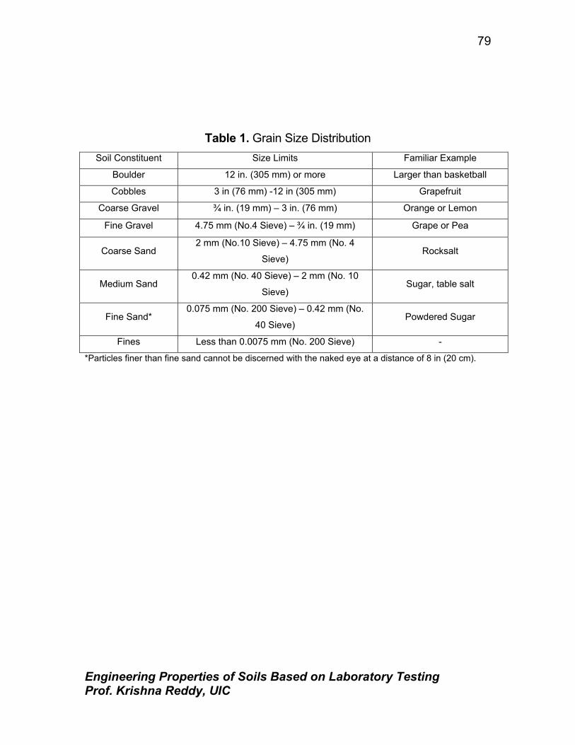
Table 1. Grain Size Distribution Soil Constituent Size Limits Familiar Example
Boulder 12 in. (305 mm) or more Larger than basketball
Cobbles 3 in (76 mm) -12 in (305 mm) Grapefruit
Coarse Gravel ¾ in. (19 mm) – 3 in. (76 mm) Orange or Lemon
Fine Gravel 4.75 mm (No.4 Sieve) – ¾ in. (19 mm) Grape or Pea
Coarse Sand 2 mm (No.10 Sieve) – 4.75 mm (No. 4
Sieve) Rocksalt
Medium Sand 0.42 mm (No. 40 Sieve) – 2 mm (No. 10
Sieve) Sugar, table salt
Fine Sand* 0.075 mm (No. 200 Sieve) – 0.42 mm (No.
40 Sieve) Powdered Sugar
Fines Less than 0.0075 mm (No. 200 Sieve) -
*Particles finer than fine sand cannot be discerned with the naked eye at a distance of 8 in (20 cm).

Engineering Properties of Soils Based on Laboratory Testing Prof. Krishna Reddy, UIC
80
Figure 1. Shape of Coarse-Grained Soil Particles
Rounded Subrounded
Angular Subangular
Table 2. Criteria for Describing Shape of Coarse-Grained Soil Particles
Description Criteria
Angular Particles have sharp edges and relatively plane sides with unpolished
surfaces.
Subangular Particles are similar to angular description, but have rounded edges.
Subrounded Particles have nearly plane sides, but have well-rounded corners and
edges.
Rounded Particles have smoothly curved sides and no edges.

Engineering Properties of Soils Based on Laboratory Testing Prof. Krishna Reddy, UIC
81
Table (3a). Criteria for Describing Dry Strength
Description Criteria
None The dry specimen ball crumbles into powder with the slightest handling
pressure.
Low The dry specimen crumbles into powder with some pressure form fingers.
Medium The dry specimen breaks into pieces or crumbles with moderate finger
pressure.
High The dry specimen cannot be broken with finger pressure. Specimen will
break into pieces between thumb and a hard surface.
Very High The dry specimen cannot be broken between the thumb and a hard
surface.
Table (3b). Criteria for Describing Dilatancy of a Soil Sample
Description Criteria
None There is no visible change in the soil samples.
Slow Water slowly appears and remains on the surface during shaking or water
slowly disappears upon squeezing.
Rapid Water quickly appears on the surface during shaking and quickly
disappears upon squeezing.

Engineering Properties of Soils Based on Laboratory Testing Prof. Krishna Reddy, UIC
82
Table (3c). Criteria for Describing Soil Plasticity
Description Criteria
Non-plastic A 1/8” (3-mm) thread cannot be rolled at any water content.
Low The thread is difficult to roll and a cohesive mass cannot be formed when
drier than the plastic limit.
Medium The thread is easy to roll and little time is needed to reach the plastic limit.
The thread cannot be re-rolled after the plastic limit is reached. The mass
crumbles when it is drier than the plastic limit.
High
Considerable time is needed, rolling and kneading the sample, to reach
the plastic limit. The thread can be rerolled and reworked several times
before reaching the plastic limit. A mass can be formed when the sample
is drier than the plastic limit
Note: The plastic limit is the water content at which the soil begins to break apart and crumbles when rolled into threads 1/8” in diameter.
Table (3d). Criteria for Describing Soil Toughness
Description Criteria
Low Only slight pressure is needed to roll the thread to the plastic limit. The
thread and mass are weak and soft.
Medium Moderate pressure is needed to roll the thread to near the plastic limit.
The thread and mass have moderate stiffness.
High Substantial pressure is needed to roll the thread to near the plastic limit.
The thread and mass are very stiff.

Engineering Properties of Soils Based on Laboratory Testing Prof. Krishna Reddy, UIC
83
Table 4. Identification of Inorganic Fine-Grained Soils
Soil Symbol Dry Strength Dilatancy Toughness
ML None or Low Slow to Rapid Low or thread cannot be formed
CL Medium to High None to Slow Medium
MH Low to Medium None to Slow Low to Medium
CH High to Very High None High
Note: ML = Silt; CL = Lean Clay (low plasticity clay); MH = Elastic Soil; CH = Fat Clay (high plasticity clay). The terms ‘lean’ and ‘fat’ may not be used in certain geographic regions (midwest).

Engineering Properties of Soils Based on Laboratory Testing Prof. Krishna Reddy, UIC
84
Table 5. Criteria for Describing Soil Moisture Conditions
Description Criteria
Dry Soil is dry to the touch, dusty, a clear absence of moisture
Moist Soil is damp, slight moisture; soil may begin to retain molded form
Wet Soil is clearly wet; water is visible when sample is squeezed
Saturated Water is easily visible and drains freely from the sample

Engineering Properties of Soils Based on Laboratory Testing Prof. Krishna Reddy, UIC
85
EXAMPLE DATA

Engineering Properties of Soils Based on Laboratory Testing Prof. Krishna Reddy, UIC
86
VISUAL SOIL CLASSIFICATION DATA SHEET
Soil Number: Soil A Classified by: RES Date: 09-29-02 1. Color brown__ 2. Odor none__ 3. Texture Coarse_ 4. Major soil constituent : gravel 5. Minor soil constituents: Sand, fines Approx. % by Type weight gravel 60 sand 30_ fines _10_ 6. For coarse-grained soils: Gradation: well graded Particle Shape: subrounded____ 7. For fine-grained soils: Dry Strength Dilatancy Plasticity Toughness Soil Symbol 8. Moisture Condition: dry___ Classification: Brown gravel, some sand, trace fines, well graded, subrounded, dry

Engineering Properties of Soils Based on Laboratory Testing Prof. Krishna Reddy, UIC
87
VISUAL SOIL CLASSIFICATION
DATA SHEET Soil Number: Soil B Classified by: RES Date: 09-27-02 1. Color gray__ 2. Odor none__ 3. Texture _coarse___ 4. Major soil constituent: __sand___ 5. Minor soil constituents: gravel, fines Approx. % by Type weight sand 80 fine gravel 15 fines 5 6. For coarse-grained soils: Gradation: poorly graded Particle Shape: rounded 7. For fine-grained soils: Dry Strength Dilatancy Plasticity Toughness Soil Symbol 8. Moisture Condition: dry___ Classification:
Gray sand, little fine gravel, trace fines, poorly graded, rounded, dry

Engineering Properties of Soils Based on Laboratory Testing Prof. Krishna Reddy, UIC
88
VISUAL SOIL CLASSIFICATION DATA SHEET
Soil Number: Soil C Classified by: RES Date: 09-29-02 1. Color gray__ 2. Odor none__ 3. Texture fine-grained_ 4. Major soil constituent : fines 5. Minor soil constituents: Fine Sand Approx. % by Type weight Fines 95 Fine Sand 5_ __ 6. For coarse-grained soils: Gradation: Particle Shape: 7. For fine-grained soils: Dry strength high Dilatancy none Plasticity medium Toughness medium Soil Symbol CL 8. Moisture Condition: moist___ Classification: Gray silty clay, trace fine sand, medium plasticity, moist, CL

Engineering Properties of Soils Based on Laboratory Testing Prof. Krishna Reddy, UIC
89
BLANK DATA SHEETS
Engineering Properties of Soils Based on Laboratory Testing Prof. Krishna Reddy, UIC
90
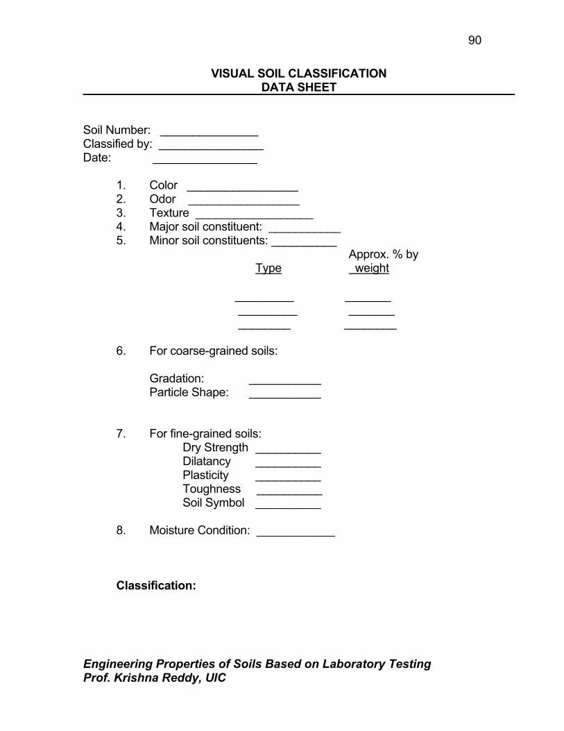
VISUAL SOIL CLASSIFICATION DATA SHEET Soil Number: _______________ Classified by: ________________ Date: ________________ 1. Color _________________ 2. Odor _________________ 3. Texture __________________ 4. Major soil constituent: ___________ 5. Minor soil constituents: __________ Approx. % by Type weight _________ _______ _________ _______ ________ ________ 6. For coarse-grained soils: Gradation: ___________ Particle Shape: ___________ 7. For fine-grained soils: Dry Strength __________ Dilatancy __________ Plasticity __________ Toughness __________ Soil Symbol __________ 8. Moisture Condition: ____________ Classification:

Engineering Properties of Soils Based on Laboratory Testing Prof. Krishna Reddy, UIC
91
EXPERIMENT 9 MOISTURE-DENSITY RELATION (COMPACTION) TEST
Purpose:
This laboratory test is performed to determine the relationship between the
moisture content and the dry density of a soil for a specified compactive effort.
The compactive effort is the amount of mechanical energy that is applied to the
soil mass. Several different methods are used to compact soil in the field, and
some examples include tamping, kneading, vibration, and static load compaction.
This laboratory will employ the tamping or impact compaction method using the
type of equipment and methodology developed by R. R. Proctor in 1933,
therefore, the test is also known as the Proctor test.
Two types of compaction tests are routinely performed: (1) The Standard
Proctor Test, and (2) The Modified Proctor Test. Each of these tests can be
performed in three different methods as outlined in the attached Table 1. In the
Standard Proctor Test, the soil is compacted by a 5.5 lb hammer falling a
distance of one foot into a soil filled mold. The mold is filled with three equal
layers of soil, and each layer is subjected to 25 drops of the hammer. The
Modified Proctor Test is identical to the Standard Proctor Test except it employs,
a 10 lb hammer falling a distance of 18 inches, and uses five equal layers of soil
instead of three. There are two types of compaction molds used for testing. The
smaller type is 4 inches in diameter and has a volume of about 1/30 ft3 (944 cm3),
and the larger type is 6 inches in diameter and has a volume of about 1/13.333 ft3
(2123 cm3). If the larger mold is used each soil layer must receive 56 blows
instead of 25 (See Table 1).

Engineering Properties of Soils Based on Laboratory Testing Prof. Krishna Reddy, UIC
92
Table 1 Alternative Proctor Test Methods
Standard Proctor ASTM 698
Modified Proctor ASTM 1557
Method A Method B Method C Method A Method B Method C
Material ≤ 20%
Retained on No.4 Sieve
>20% Retained on
No.4 ≤ 20%
Retained on 3/8” Sieve
>20% Retained on
No.3/8” <30%
Retained on 3/4” Sieve
≤ 20% Retained on No.4 Sieve
>20% Retained on
No.4 ≤ 20%
Retained on 3/8” Sieve
>20% Retained on
No.3/8” <30%
Retained on 3/4” Sieve
For test sample, use soil passing
Sieve No.4 3/8” Sieve ¾” Sieve Sieve No.4 3/8” Sieve ¾” Sieve
Mold 4” DIA 4” DIA 6” DIA 4” DIA 4” DIA 6” DIA No. of Layers 3 3 3 5 5 5
No. of blows/layer 25 25 56 25 25 56
Note: Volume of 4” diameter mold = 944 cm3 , Volume of 6” diameter mold = 2123 cm3
(verify these values prior to testing)

Engineering Properties of Soils Based on Laboratory Testing Prof. Krishna Reddy, UIC
93
Standard Reference:
ASTM D 698 - Standard Test Methods for Laboratory Compaction
Characteristics of Soil Using Standard Effort (12,400 ft-lbs/ft3 (600 KN-m/m3))
ASTM D 1557 - Standard Test Methods for Laboratory Compaction
Characteristics of Soil Using Modified Effort (56,000 ft-lbs/ft3 (2,700 KN-m/m3))
Significance:
Mechanical compaction is one of the most common and cost effective
means of stabilizing soils. An extremely important task of geotechnical engineers
is the performance and analysis of field control tests to assure that compacted
fills are meeting the prescribed design specifications. Design specifications
usually state the required density (as a percentage of the “maximum” density
measured in a standard laboratory test), and the water content. In general, most
engineering properties, such as the strength, stiffness, resistance to shrinkage,
and imperviousness of the soil, will improve by increasing the soil density.
The optimum water content is the water content that results in the greatest
density for a specified compactive effort. Compacting at water contents higher
than (wet of ) the optimum water content results in a relatively dispersed soil
structure (parallel particle orientations) that is weaker, more ductile, less
pervious, softer, more susceptible to shrinking, and less susceptible to swelling
than soil compacted dry of optimum to the same density. The soil compacted
lower than (dry of) the optimum water content typically results in a flocculated soil
structure (random particle orientations) that has the opposite characteristics of
the soil compacted wet of the optimum water content to the same density.

Engineering Properties of Soils Based on Laboratory Testing Prof. Krishna Reddy, UIC
94
Equipment: Molds, Manual rammer, Extruder, Balance, Drying oven, Mixing pan,
Trowel, #4 sieve, Moisture cans, Graduated cylinder, Straight Edge.

Engineering Properties of Soils Based on Laboratory Testing Prof. Krishna Reddy, UIC
95

Engineering Properties of Soils Based on Laboratory Testing Prof. Krishna Reddy, UIC
96
Test Procedure:
(1) Depending on the type of mold you are using obtain a sufficient
quantity of air-dried soil in large mixing pan. For the 4-inch mold
take approximately 10 lbs, and for the 6-inch mold take roughly 15
lbs. Pulverize the soil and run it through the # 4 sieve.
(2) Determine the weight of the soil sample as well as the weight of the
compaction mold with its base (without the collar) by using the
balance and record the weights.
(3) Compute the amount of initial water to add by the following method:
(a) Assume water content for the first test to be 8 percent.
(b) Compute water to add from the following equation:
( )100
8gramsinmasssoilml)(in addtowater =
Where “water to add” and the “soil mass” are in grams. Remember
that a gram of water is equal to approximately one milliliter of water.
(4) Measure out the water, add it to the soil, and then mix it thoroughly
into the soil using the trowel until the soil gets a uniform color (See
Photos B and C).
(5) Assemble the compaction mold to the base, place some soil in the
mold and compact the soil in the number of equal layers specified by
the type of compaction method employed (See Photos D and E).
The number of drops of the rammer per layer is also dependent
upon the type of mold used (See Table 1). The drops should be
applied at a uniform rate not exceeding around 1.5 seconds per
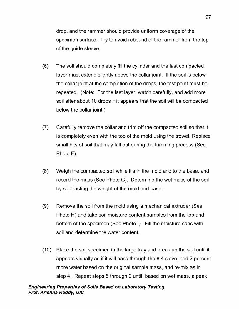
Engineering Properties of Soils Based on Laboratory Testing Prof. Krishna Reddy, UIC
97
drop, and the rammer should provide uniform coverage of the
specimen surface. Try to avoid rebound of the rammer from the top
of the guide sleeve.
(6) The soil should completely fill the cylinder and the last compacted
layer must extend slightly above the collar joint. If the soil is below
the collar joint at the completion of the drops, the test point must be
repeated. (Note: For the last layer, watch carefully, and add more
soil after about 10 drops if it appears that the soil will be compacted
below the collar joint.)
(7) Carefully remove the collar and trim off the compacted soil so that it
is completely even with the top of the mold using the trowel. Replace
small bits of soil that may fall out during the trimming process (See
Photo F).
(8) Weigh the compacted soil while it’s in the mold and to the base, and
record the mass (See Photo G). Determine the wet mass of the soil
by subtracting the weight of the mold and base.
(9) Remove the soil from the mold using a mechanical extruder (See
Photo H) and take soil moisture content samples from the top and
bottom of the specimen (See Photo I). Fill the moisture cans with
soil and determine the water content.
(10) Place the soil specimen in the large tray and break up the soil until it
appears visually as if it will pass through the # 4 sieve, add 2 percent
more water based on the original sample mass, and re-mix as in
step 4. Repeat steps 5 through 9 until, based on wet mass, a peak

Engineering Properties of Soils Based on Laboratory Testing Prof. Krishna Reddy, UIC
98
value is reached followed by two slightly lesser compacted soil
masses.
Analysis:
(1) Calculate the moisture content of each compacted soil specimen by
using the average of the two water contents.
(2) Compute the wet density in grams per cm3 of the compacted soil
sample by dividing the wet mass by the volume of the mold used.
(3) Compute the dry density using the wet density and the water content
determined in step 1. Use the following formula:
w1ρ
dρ +=
where: w = moisture content in percent divided by 100, and ρ = wet
density in grams per cm3.
(4) Plot the dry density values on the y-axis and the moisture contents
on the x-axis. Draw a smooth curve connecting the plotted points.
(5) On the same graph draw a curve of complete saturation or “zero air
voids curve”. The values of dry density and corresponding moisture
contents for plotting the curve can be computed from the following
equation:
100G1w
sd
wsat ×
−
ρρ
=
or
+
=
Gsw
wd 1
100
ρρ

Engineering Properties of Soils Based on Laboratory Testing Prof. Krishna Reddy, UIC
99
where:
ρd = dry density of soil grams per cm3
Gs = specific gravity of the soil being tested (assume 2.70 if not given)
ρw = density of water in grams per cm3 (approximately1 g/cm3)
wsat = moisture content in percent for complete saturation.
Example Calculations:
Gs=2.7 (assumed)
ρw=1.0 g/cm3
Assumed wsat% Calculated ρd (g/cm3)
8 2.22
10 2.13
12 2.04
14 1.96
16 1.89
18 1.82
(6) Identify and report the optimum moisture content and the maximum dry
density. Make sure that you have recorded the method of compaction
used (e.g., Standard Proctor, Method A) on data sheet.
Engineering Properties of Soils Based on Laboratory Testing Prof. Krishna Reddy, UIC
100
EXAMPLE DATA

Engineering Properties of Soils Based on Laboratory Testing Prof. Krishna Reddy, UIC
101
Moisture-Density (Compaction) Test Data Sheets
Test Method: Standard Proctor, Method A (ASTM 698)
Date Tested: October 05, 2002 Tested By: CEMM315 Class, Group A Project Name: CEMM315 Lab Sample Number: Bag-1, 2’-6’ Visual Classification of Soil: Gray silty clay, trace fine sand, low plasticity, moist, CL Water Content Determination:
Compacted Soil - Sample no. 1 2 3 Water content - Sample no. 1A 1B 2A 2B 3A 3B Moisture can number - Lid number 1 2 3 4 5 6
MC = Mass of empty, clean can + lid (grams) 7.78 7.83 7.71 7.9 7.5 7.9
MCMS = Mass of can, lid, and moist soil (grams) 11.78 11.05 10.71 11 . 1 10.7 12 .0
MCDS = Mass of can, lid, and dry soil (grams) 11.48 10.81 10.41 10.75 10.3 11.52
MS = Mass of soil solids (grams) 3.70 2.98 2.7 2.85 2.84 3.62
MW = Mass of pore water (grams) 0.29 0.24 0.30 0.35 0.40 0.53
w = Water content, w% 7.9 8.1 11 . 1 10.9 12.5 13.1
Compacted Soil - Sample no. 4 5 6 Water content - Sample no. 4A 4B 5A 5B 6A 6B Moisture can number - Lid number 7 8 9 10
MC = Mass of empty, clean can + lid (grams) 8.1 7.6 7.7 7.65
MCMS = Mass of can, lid, and moist soil (grams) 11. 1 10.2 10.3 10.33
MCDS = Mass of can, lid, and dry soil (grams) 10.70 9.84 10.02 9.92
MS = Mass of soil solids (grams) 2.60 2.24 2.32 2.27
MW = Mass of pore water (grams) 0.40 0.35 0.4 0.39
w = Water content, w% 15.3 16.0 17. 1 17.6

Engineering Properties of Soils Based on Laboratory Testing Prof. Krishna Reddy, UIC
102
Density Determination:
Mold Volume=944 cm3
Compacted Soil - Sample no. 1 2 3 4 5 6
w = Assumed water content, w% 10 12 14 16 18
Actual average water content, w% 8.0 11.0 12.8 15.65 17
Mass of compacted soil and mold
(grams) 3457.2 3721.2 3909.0 3782.5 3715.2
Mass of mold (grams) 1933 1933 1976.0 1849.5 1782.2
Wet mass of soil in mold (grams) 1524.2 1788.2 2176 2149 2082
Wet density, ρ , (g/cm3) 1.615 1.894 2.093 1.959 1.888
Dry density, ρd , (g/cm3) 1.50 1.71 1.86 1.69 1.61
1.0
1.2
1.4
1.6
1.8
2.0
2.2
2.4
0 5 10 15 20
Water Content, w%
Dry
Den
sity
, g/c
m3
OMC
ρdmax
Zero Air Voids Curve(Gs=2.7 assumed)
Optimum Moisture Content = 13.1 %
Maximum Dry Density = 1.87 g/cm3

Engineering Properties of Soils Based on Laboratory Testing Prof. Krishna Reddy, UIC
103
BLANK DATA SHEETS

Engineering Properties of Soils Based on Laboratory Testing Prof. Krishna Reddy, UIC
104
Moisture-Density (Compaction) Test Data Sheets
Test Method: Date Tested: Tested By: Project Name: Sample Number: Visual Classification of Soil:
Water Content Determination:
Compacted Soil - Sample no. 1 2 3 Water content - Sample no. 1A 1B 2A 2B 3A 3B Moisture can number - Lid number MC = Mass of empty, clean can + lid (grams)
MCMS = Mass of can, lid, and moist soil (grams)
MCDS = Mass of can, lid, and dry soil (grams)
MS = Mass of soil solids (grams)
MW = Mass of pore water (grams) W = Water content, w%
Compacted Soil - Sample no. 4 5 6 Water content - Sample no. 4A 4B 5A 5B 6A 6B Moisture can number - Lid number MC = Mass of empty, clean can + lid (grams)
MCMS = Mass of can, lid, and moist soil (grams)
MCDS = Mass of can, lid, and dry soil (grams)
MS = Mass of soil solids (grams)
MW = Mass of pore water (grams) W = Water content, w%

Engineering Properties of Soils Based on Laboratory Testing Prof. Krishna Reddy, UIC
105
Density Determination:
Volume of mold= Compacted Soil - Sample no. 1 2 3 4 5 6 w = Assumed water content, w% Actual average water content, w% Mass of compacted soil and mold (grams) Mass of mold (grams) Wet mass of soil in mold (grams) Wet density, ρ , (kg/m
3)
Dry density, ρd , (kg/m3)
Optimum Moisture Content = _________________ %
Maximum Dry Density = ___________________ g/cm3
1.0
1.2
1.4
1.6
1.8
2.0
2.2
2.4
2.6
5 10 15 20 25
Water Content, w%
Dry
Den
sity
(g/c
m3 )

Engineering Properties of Soils Based on Laboratory Testing Prof. Krishna Reddy, UIC
106
EXPERIMENT 10 PERMEABILITY (HYDRAULIC CONDUCTIVITY) TEST
CONSTANT HEAD METHOD Purpose:
The purpose of this test is to determine the permeability (hydraulic
conductivity) of a sandy soil by the constant head test method. There are
two general types of permeability test methods that are routinely performed
in the laboratory: (1) the constant head test method, and (2) the falling head
test method. The constant head test method is used for permeable soils
(k>10-4 cm/s) and the falling head test is mainly used for less permeable soils
(k<10-4 cm/s).
Standard Reference:
ASTM D 2434 - Standard Test Method for Permeability of Granular
Soils (Constant Head) (Note: The Falling Head Test Method is not
standardized)
Significance:
Permeability (or hydraulic conductivity) refers to the ease with which
water can flow through a soil. This property is necessary for the calculation
of seepage through earth dams or under sheet pile walls, the calculation of
the seepage rate from waste storage facilities (landfills, ponds, etc.), and the
calculation of the rate of settlement of clayey soil deposits.

Engineering Properties of Soils Based on Laboratory Testing Prof. Krishna Reddy, UIC
107
Equipment: Permeameter, Tamper, Balance, Scoop, 1000 mL Graduated
cylinders, Watch (or Stopwatch), Thermometer, Filter paper.

Engineering Properties of Soils Based on Laboratory Testing Prof. Krishna Reddy, UIC
108

Engineering Properties of Soils Based on Laboratory Testing Prof. Krishna Reddy, UIC
109
Test Procedure:
(1) Measure the initial mass of the pan along with the dry soil (M1).
(2) Remove the cap and upper chamber of the permeameter by
unscrewing the knurled cap nuts and lifting them off the tie rods.
Measure the inside diameter of upper and lower chambers. Calculate
the average inside diameter of the permeameter (D).
(3) Place one porous stone on the inner support ring in the base of the
chamber then place a filter paper on top of the porous stone (see
Photo C).
(4) Mix the soil with a sufficient quantity of distilled water to prevent the
segregation of particle sizes during placement into the permeameter.
Enough water should be added so that the mixture may flow freely
(see Photo B).
(5) Using a scoop, pour the prepared soil into the lower chamber using a
circular motion to fill it to a depth of 1.5 cm. A uniform layer should be
formed.
(6) Use the tamping device to compact the layer of soil. Use
approximately ten rams of the tamper per layer and provide uniform
coverage of the soil surface. Repeat the compaction procedure until
the soil is within 2 cm. of the top of the lower chamber section (see
Photo D).

Engineering Properties of Soils Based on Laboratory Testing Prof. Krishna Reddy, UIC
110
(7) Replace the upper chamber section, and don’t forget the rubber
gasket that goes between the chamber sections. Be careful not to
disturb the soil that has already been compacted. Continue the
placement operation until the level of the soil is about 2 cm. below the
rim of the upper chamber. Level the top surface of the soil and place
a filter paper and then the upper porous stone on it (see Photo E).
(8) Place the compression spring on the porous stone and replace the
chamber cap and its sealing gasket. Secure the cap firmly with the
cap nuts (see Photo F).
(9) Measure the sample length at four locations around the circumference
of the permeameter and compute the average length. Record it as the
sample length.
(10) Keep the pan with remaining soil in the drying oven.
(11) Adjust the level of the funnel to allow the constant water level in it to
remain a few inches above the top of the soil.
(12) Connect the flexible tube from the tail of the funnel to the bottom outlet
of the permeameter and keep the valves on the top of the
permeameter open (see Photo G).
(13) Place tubing from the top outlet to the sink to collect any water that
may come out (see Photo G).

Engineering Properties of Soils Based on Laboratory Testing Prof. Krishna Reddy, UIC
111
(14) Open the bottom valve and allow the water to flow into the
permeameter.
(15) As soon as the water begins to flow out of the top control (deairing)
valve, close the control valve, letting water flow out of the outlet for
some time.
(16) Close the bottom outlet valve and disconnect the tubing at the bottom.
Connect the funnel tubing to the top side port (see Photo H).
(17) Open the bottom outlet valve and raise the funnel to a convenient
height to get a reasonable steady flow of water.
(18) Allow adequate time for the flow pattern to stabilize (see Photo I).
(19) Measure the time it takes to fill a volume of 750 - 1000 mL using the
graduated cylinder, and then measure the temperature of the water.
Repeat this process three times and compute the average time,
average volume, and average temperature. Record the values as t,
Q, and T, respectively (see Photo I).
(20) Measure the vertical distance between the funnel head level and the
chamber outflow level, and record the distance as h.
(21) Repeat step 17 and 18 with different vertical distances.
(22) Remove the pan from the drying oven and measure the final mass of
the pan along with the dry soil (M2).

Engineering Properties of Soils Based on Laboratory Testing Prof. Krishna Reddy, UIC
112
Analysis:
(1) Calculate the permeability, using the following equation:
AthQL
TK =
Where:
KT = coefficient of permeability at temperature T, cm/sec.
L = length of specimen in centimeters
t = time for discharge in seconds
Q = volume of discharge in cm3 (assume 1 mL = 1 cm3)
A = cross-sectional area of permeameter (= 2D4π , D= inside
diameter of the permeameter)
h = hydraulic head difference across length L, in cm of water; or it is
equal to the vertical distance between the constant funnel head level
and the chamber overflow level.
(2) The viscosity of the water changes with temperature. As temperature
increases viscosity decreases and the permeability increases. The
coefficient of permeability is standardized at 20°C, and the
permeability at any temperature T is related to K20 by the following
ratio:
20ηTη
TK20K =
Where:
ηT and η20 are the viscosities at the temperature T of the test and at
20°C, respectively. From Table 1 obtain the viscosities and compute
K20.

Engineering Properties of Soils Based on Laboratory Testing Prof. Krishna Reddy, UIC
113
(3) Compute the volume of soil used from: V = LA.
(4) Compute the mass of dry soil used in permeameter (M) = initial mass -
final mass:
M = M1-M2
(5) Compute the dry density (ρd) of soil
VM
dρ =

Engineering Properties of Soils Based on Laboratory Testing Prof. Krishna Reddy, UIC
114
Table 1. Properties of Distilled Water (η = absolute)
TemperatureCo
Density (g/cm3)
Viscosity(Poise*)
4 1.00000 0.01567 16 0.99897 0.01111 17 0.99880 0.01083 18 0.99862 0.01056 19 0.99844 0.01030 20 0.99823 0.01005 21 0.99802 0.00981 22 0.99780 0.00958 23 0.99757 0.00936 24 0.99733 0.00914 25 0.99708 0.00894 26 0.99682 0.00874 27 0.99655 0.00855 28 0.99627 0.00836 29 0. 99598 0.00818 30 0. 99568 0.00801
*Poisescm
g2cm
sdyne⋅
=⋅=
Engineering Properties of Soils Based on Laboratory Testing Prof. Krishna Reddy, UIC
115
EXAMPLE DATA
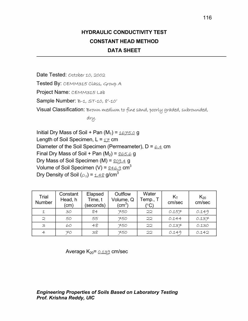
Engineering Properties of Soils Based on Laboratory Testing Prof. Krishna Reddy, UIC
116
HYDRAULIC CONDUCTIVITY TEST CONSTANT HEAD METHOD
DATA SHEET
Date Tested: October 10, 2002 Tested By: CEMM315 Class, Group A
Project Name: CEMM315 Lab
Sample Number: B-1, ST-10, 8’-10’
Visual Classification: Brown medium to fine sand, poorly graded, subrounded,
dry.
Initial Dry Mass of Soil + Pan (M1) = 1675.0 g Length of Soil Specimen, L = 17 cm Diameter of the Soil Specimen (Permeameter), D = 6.4 cm Final Dry Mass of Soil + Pan (M2) = 865.6 g Dry Mass of Soil Specimen (M) = 809.4 g Volume of Soil Specimen (V) = 846.9 cm3 Dry Density of Soil (ρd) = 1.48 g/cm3
Trial Number
Constant Head, h
(cm)
Elapsed Time, t
(seconds)
Outflow Volume, Q
(cm3)
Water Temp., T
(°C)
KT cm/sec
K20 cm/sec
1 30 84 750 22 0.157 0.149 2 50 55 750 22 0.144 0.137 3 60 48 750 22 0.137 0.130 4 70 38 750 22 0.149 0.142
Average K20= 0.139 cm/sec

Engineering Properties of Soils Based on Laboratory Testing Prof. Krishna Reddy, UIC
117
BLANK DATA SHEETS

Engineering Properties of Soils Based on Laboratory Testing Prof. Krishna Reddy, UIC
118
HYDRAULIC CONDUCTIVITY TEST
CONSTANT HEAD METHOD
DATA SHEET Date Tested: Tested By: Project Name: Sample Number: Visual Classification: Initial Dry Mass of Soil + Pan (M1) = __________________ g Length of Soil Specimen, L = _________________ cm Diameter of the Soil Specimen (Permeameter), D = _____________ cm Final Dry Mass of Soil + Pan (M2) = _________________ g Dry Mass of Soil Specimen (M) = _____________________ g Volume of Soil Specimen (V) = ___________________ cm3 Dry Density of Soil (ρd) = __________________ g/cm3
Trial Number
Constant Head, h
(cm)
Elapsed Time, t
(seconds)
Outflow Volume, Q
(cm3)
Water Temp., T
(°C) KT K20
1 2 3 4
Average K20= ______________________ cm/sec

Engineering Properties of Soils Based on Laboratory Testing Prof. Krishna Reddy, UIC
119
EXPERIMENT 11 CONSOLIDATION TEST
Purpose:
This test is performed to determine the magnitude and rate of volume
decrease that a laterally confined soil specimen undergoes when subjected
to different vertical pressures. From the measured data, the consolidation
curve (pressure-void ratio relationship) can be plotted. This data is useful in
determining the compression index, the recompression index and the
preconsolidation pressure (or maximum past pressure) of the soi. In
addition, the data obtained can also be used to determine the coefficient of
consolidation and the coefficient of secondary compression of the soil.
Standard Reference:
ASTM D 2435 - Standard Test Method for One-Dimensional
Consolidation Properties of Soils.
Significance:
The consolidation properties determined from the consolidation test
are used to estimate the magnitude and the rate of both primary and
secondary consolidation settlement of a structure or an earthfill. Estimates of
this type are of key importance in the design of engineered structures and
the evaluation of their performance.
Equipment: Consolidation device (including ring, porous stones, water reservoir, and load
plate), Dial gauge (0.0001 inch = 1.0 on dial), Sample trimming device, glass
plate, Metal straight edge, Clock, Moisture can, Filter paper.

Engineering Properties of Soils Based on Laboratory Testing Prof. Krishna Reddy, UIC
120
Engineering Properties of Soils Based on Laboratory Testing Prof. Krishna Reddy, UIC
121
Test Procedure:
(1) Weigh the empty consolidation ring together with glass plate.
(2) Measure the height (h) of the ring and its inside diameter (d).
(3) Extrude the soil sample from the sampler, generally thin-walled Shelby
tube. Determine the initial moisture content and the specific gravity of
the soil as per Experiments 1 and 4, respectively (Use the data sheets
from these experiments to record all of the data).
(4) Cut approximately a three-inch long sample. Place the sample on the
consolidation ring and cut the sides of the sample to be approximately
the same as the outside diameter of the ring. Rotate the ring and pare
off the excess soil by means of the cutting tool so that the sample is
reduced to the same inside diameter of the ring. It is important to keep
the cutting tool in the correct horizontal position during this process.
(5) As the trimming progresses, press the sample gently into the ring and
continue until the sample protrudes a short distance through the
bottom of the ring. Be careful throughout the trimming process to
insure that there is no void space between the sample and the ring.
(6) Turn the ring over carefully and remove the portion of the soil
protruding above the ring. Using the metal straight edge, cut the soil
surface flush with the surface of the ring. Remove the final portion
with extreme care.

Engineering Properties of Soils Based on Laboratory Testing Prof. Krishna Reddy, UIC
122
(7) Place the previously weighed Saran-covered glass plate on the freshly
cut surface, turn the ring over again, and carefully cut the other end in
a similar manner.
(8) Weigh the specimen plus ring plus glass plate.
(9) Carefully remove the ring with specimen from the Saran-covered glass
plate and peel the Saran from the specimen surface. Center the
porous stones that have been soaking, on the top and bottom surfaces
of the test specimen. Place the filter papers between porous stones
and soil specimen. Press very lightly to make sure that the stones
adhere to the sample. Lower the assembly carefully into the base of
the water reservoir. Fill the water reservoir with water until the
specimen is completely covered and saturated.
(10) Being careful to prevent movement of the ring and porous stones,
place the load plate centrally on the upper porous stone and adjust the
loading device.
(11) Adjust the dial gauge to a zero reading.
(12) With the toggle switch in the down (closed) position, set the pressure
gauge dial (based on calibration curve) to result in an applied pressure
of 0.5 tsf (tons per square foot).
(13) Simultaneously, open the valve (by quickly lifting the toggle switch to
the up (open) position) and start the timing clock.

Engineering Properties of Soils Based on Laboratory Testing Prof. Krishna Reddy, UIC
123
(14) Record the consolidation dial readings at the elapsed times given on
the data sheet.
(15) Repeat Steps 11 to 13 for different preselected pressures (generally
includes loading pressures of 1.0, 2.0, 4.0, 8.0, and 16.0 tsf and
unloading pressures of 8.0, 4.0, 2.0, 1.0 and 0.5 tsf)
(16) At the last elapsed time reading, record the final consolidation dial
reading and time, release the load, and quickly disassemble the
consolidation device and remove the specimen. Quickly but carefully
blot the surfaces dry with paper toweling. (The specimen will tend to
absorb water after the load is released.)
(17) Place the specimen and ring on the Saran-covered glass plate and,
once again, weigh them together.
(18) Weigh an empty large moisture can and lid.
(19) Carefully remove the specimen from the consolidation ring, being sure
not to lose too much soil, and place the specimen in the previously
weighed moisture can. Place the moisture can containing the
specimen in the oven and let it dry for 12 to 18 hours.
(20) Weigh the dry specimen in the moisture can.
Analysis:
(1) Calculate the initial water content and specific gravity of the soil.
Engineering Properties of Soils Based on Laboratory Testing Prof. Krishna Reddy, UIC
124
(2) For each pressure increment, construct a semilog plot of the
consolidation dial readings versus the log time (in minutes).
Determine D0, D50, D100, and the coefficient of consolidation (cv) using
Casagrande’s logarithm of time fitting method. See example data.
Also calculate the coefficient of secondary compression based on
these plots.
(3) Calculate the void ratio at the end of primary consolidation for each
pressure increment (see example data). Plot log pressure versus void
ratio. Based on this plot, calculate compression index, recompression
index and preconsolidation pressure (maximum past pressure).
(4) Summarize and discuss the results.

Engineering Properties of Soils Based on Laboratory Testing Prof. Krishna Reddy, UIC
125
EXAMPLE DATA

Engineering Properties of Soils Based on Laboratory Testing Prof. Krishna Reddy, UIC
126
Consolidation Test Data Sheets
Date Tested: October 05, 2002 Tested By: CEMM315 Class, Group A Project Name: CEMM315 Lab Sample Number: GB-08-ST-13’-15’ Visual Classification: Gray silty clay Before test Consolidation type = Floating type Mass of the ring + glass plate = 465.9 g Inside diameter of the ring = 6.3 cm Height of specimen, Hi = 2.7 cm Area of specimen, A = 31.172 cm2
Mass of specimen + ring = 646.4 g Initial moisture content of specimen, wi (%) = 19.5 % Specific gravity of solids, Gs = 2.67 After test Mass of wet sample + ring + glass plate = 636.5 g Mass of can = 59.3 g Mass of can + wet soil = 229.8 g Mass of wet specimen = 170.50 g Mass of can + dry soil = 208.5 g Mass of dry specimen, Ms = 149.2 g Final moisture content of specimen, wf = 14.27 %
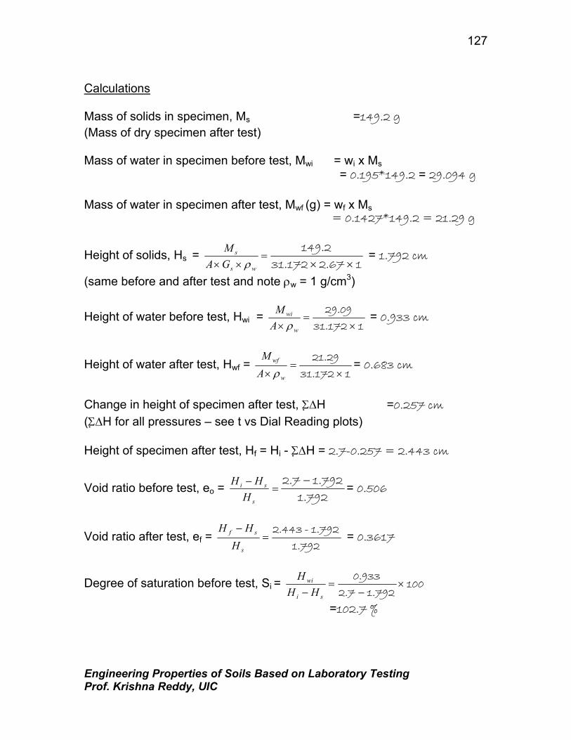
Engineering Properties of Soils Based on Laboratory Testing Prof. Krishna Reddy, UIC
127
Calculations Mass of solids in specimen, Ms =149.2 g (Mass of dry specimen after test) Mass of water in specimen before test, Mwi = wi x Ms
= 0.195*149.2 = 29.094 g Mass of water in specimen after test, Mwf (g) = wf x Ms = 0.1427*149.2 = 21.29 g
Height of solids, Hs = 12.6731.172
149.2
××=
×× ws
s
GAM
ρ = 1.792 cm
(same before and after test and note ρw = 1 g/cm3)
Height of water before test, Hwi = 131.172
29.09
×=
× w
wi
AM
ρ = 0.933 cm
Height of water after test, Hwf = 131.172
21.29
×=
× w
wf
AM
ρ= 0.683 cm
Change in height of specimen after test, Σ∆H =0.257 cm (Σ∆H for all pressures – see t vs Dial Reading plots) Height of specimen after test, Hf = Hi - Σ∆H = 2.7-0.257 = 2.443 cm
Void ratio before test, eo = 1.792
1.7922.7 −=
−
s
si
HHH = 0.506
Void ratio after test, ef = 1.792
1.792-2.443=
−
s
sf
HHH
= 0.3617
Degree of saturation before test, Si = 1001.7922.7
0.933×
−=
− si
wi
HHH
=102.7 %

Engineering Properties of Soils Based on Laboratory Testing Prof. Krishna Reddy, UIC
128
Degree of saturation after test, Sf = 1001.7922.443
0.683
HH
H
sf
wf ×−
=−
=105.08%
Dry density before test, ρd = 31.1722.7
149.2
AH
M
i
s
×=
× = 1.77 g/cm3
=(110.6 pcf)

Engineering Properties of Soils Based on Laboratory Testing Prof. Krishna Reddy, UIC
129
Table 1: Time - Settlement Data (1 unit on dial guage = 0.0001 inches) loading= ¼ tsf loading=1/8 tsf loading=1/2 tsf loading=1 tsf
time dail reading time dail reading time dail reading time dail reading 0 0 0 0 0 0 0 0
0.1 0 0.1 0 0.1 13 0.1 6 0.25 0 0.25 0 0.25 18 0.25 8 0.5 0 0.5 0 0.5 25 0.5 11.5 1 1 1 34 1 15 2 2 2 40 2 20.5 4 4 4 54 4 27 8 8 8 77 10 42
15 15 15 90 15 46 30 30 30 126 31 58 60 60 60 144.5 60 79
120 120 130 160 121 81 300 162 240 85
loading=2 tsf 1380 169 562 86 time dail reading
0 255 loading=4 tsf loading=2 tsf (unloading) loading=1 tsf (unloading)0.1 255.5 time dail reading time dail reading time dail reading
0.25 256 0 313 0 496 0 492.5 0.5 256.5 0.06 319 0.1 496 0.1 492.5 1 257 0.15 328 0.25 496 0.25 492.5 2 257.5 0.3 336 0.5 495.5 0.5 492 4 258 1 357 1 495 1 490.5 8 258.5 2 375 2 494 2 486.5
15 262.5 4 398 4 493.5 4 481.5 30 283 8 428 8 493 8 477.5 60 286 15 453 15 492.5 15 474.5
128 292.5 30 464 30 492.5 44 472.5 240 297 60 472.5 70 492.5 60 471.5 335 299 120 479.5 140 492.5 218 470.5 390 300 290 486 215 492.5 678 303 395 488
1380 303.5 1230 496 1520 304
loading=1/2 tsf (unloading) loading=1 tsf (reloading) loading=2 tsf (reloading) loading=4 tsf (reloading)
time dail reading time dail reading time dail reading time dail reading 0 470.5
0.06 469.5 0 440.5 0 442.4 0 446.5 0.5 466 0.1 440.7 0.1 442.9 0.1 446.5 1 464.5 0.25 441 0.25 443.4 0.25 446.6 2 461.5 0.5 441.2 0.5 444.4 0.5 449.5 4 458.5 1 441.5 1 445.1 1 456.5 8 454 2 441.6 2 445.3 2 465.5
15 450.5 4 441.8 4 445.4 4 473.5 30 447 8 442 8 445.9 8 481 60 444.5 15 442.1 15 446.3 17 485.5
110 443.5 30 442.4 30 446.4 30 488 930 440.5 60 442.4 60 446.5 108 490.5
120 442.4 120 446.5 947 500
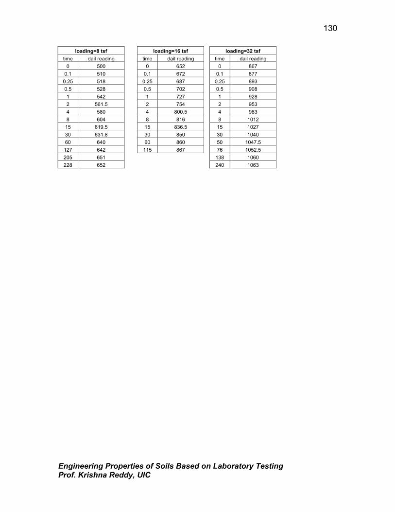
Engineering Properties of Soils Based on Laboratory Testing Prof. Krishna Reddy, UIC
130
loading=8 tsf loading=16 tsf loading=32 tsf time dail reading time dail reading time dail reading
0 500 0 652 0 867 0.1 510 0.1 672 0.1 877
0.25 518 0.25 687 0.25 893 0.5 528 0.5 702 0.5 908 1 542 1 727 1 928 2 561.5 2 754 2 953 4 580 4 800.5 4 983 8 604 8 816 8 1012
15 619.5 15 836.5 15 1027 30 631.8 30 850 30 1040 60 640 60 860 50 1047.5
127 642 115 867 76 1052.5 205 651 138 1060 228 652 240 1063

Engineering Properties of Soils Based on Laboratory Testing Prof. Krishna Reddy, UIC
131
Consolidation Test (ASTM D 2435)
Sample: GB-08-ST-13'-15'Pressure = 1/2 tsf
0
20
40
60
80
100
120
140
160
1800.01 0.1 1 10 100 1000 10000
Time (min)
Dai
l Rea
ding
(x 0
.000
1 in
)
∆Η = 0.0153 in t50=10 min
D0 = 8
D100 = 159
5.8321598
2100D0D
50D =+=+
=
Consolidation Test (ASTM D 2435)
Sample: GB-08-ST-13'-15'Pressure = 1 tsf
170
180
190
200
210
220
230
240
250
2600.01 0.1 1 10 100 1000 10000
Time (min)
Dai
l Rea
ding
(x 0
.000
1 in
)
t50 = 11.5 min∆H = 0.008 in
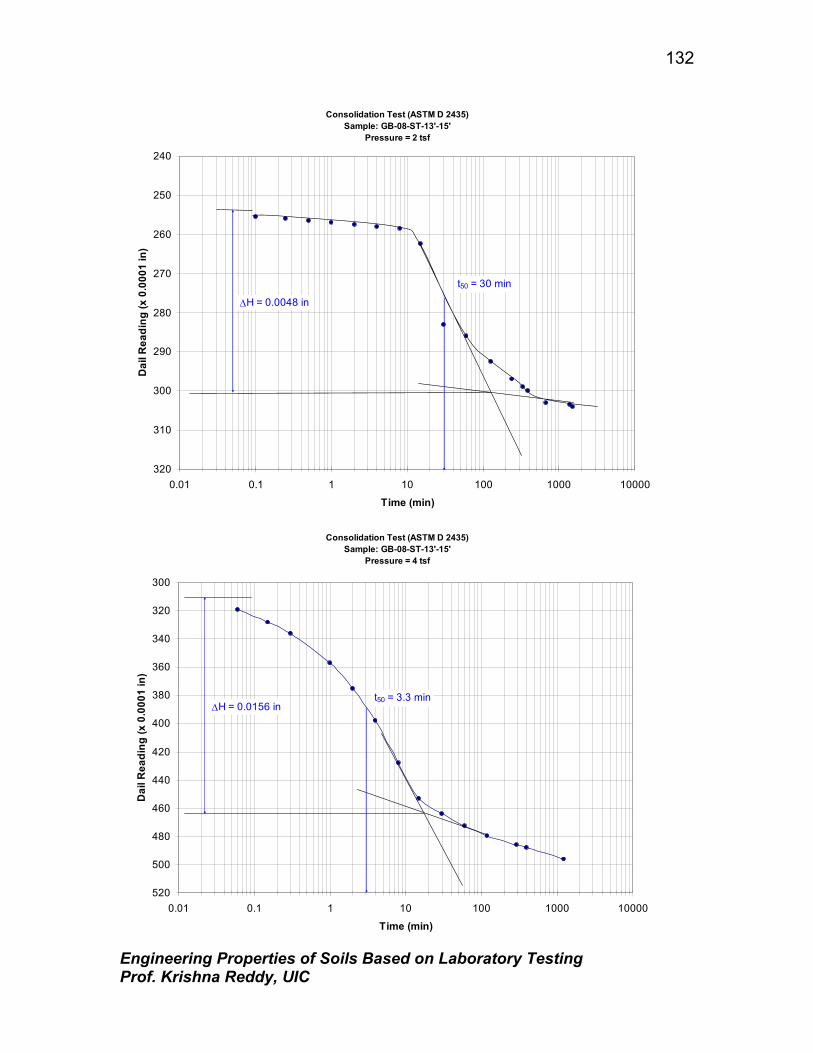
Engineering Properties of Soils Based on Laboratory Testing Prof. Krishna Reddy, UIC
132
Consolidation Test (ASTM D 2435)Sample: GB-08-ST-13'-15'
Pressure = 2 tsf
240
250
260
270
280
290
300
310
3200.01 0.1 1 10 100 1000 10000
Time (min)
Dai
l Rea
ding
(x 0
.000
1 in
)
∆H = 0.0048 in
t50 = 30 min
Consolidation Test (ASTM D 2435)
Sample: GB-08-ST-13'-15'Pressure = 4 tsf
300
320
340
360
380
400
420
440
460
480
500
5200.01 0.1 1 10 100 1000 10000
Time (min)
Dai
l Rea
ding
(x 0
.000
1 in
)
∆H = 0.0156 int50 = 3.3 min
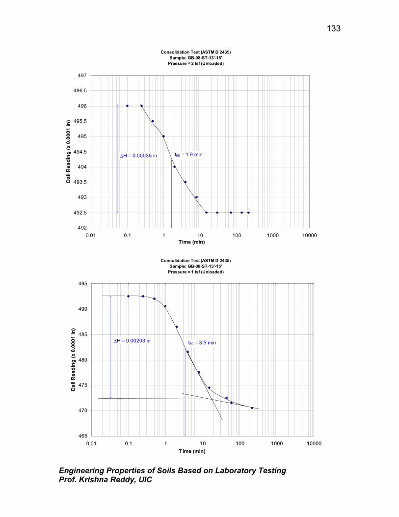
Engineering Properties of Soils Based on Laboratory Testing Prof. Krishna Reddy, UIC
133
Consolidation Test (ASTM D 2435)Sample: GB-08-ST-13'-15'
Pressure = 2 tsf (Unloaded)
492
492.5
493
493.5
494
494.5
495
495.5
496
496.5
497
0.01 0.1 1 10 100 1000 10000Time (min)
Dai
l Rea
ding
(x 0
.000
1 in
)
∆H = 0.00035 in t50 = 1.9 min
Consolidation Test (ASTM D 2435)Sample: GB-08-ST-13'-15'
Pressure = 1 tsf (Unloaded)
465
470
475
480
485
490
495
0.01 0.1 1 10 100 1000 10000Time (min)
Dai
l Rea
ding
(x 0
.000
1 in
)
t50 = 3.5 min∆H = 0.00203 in
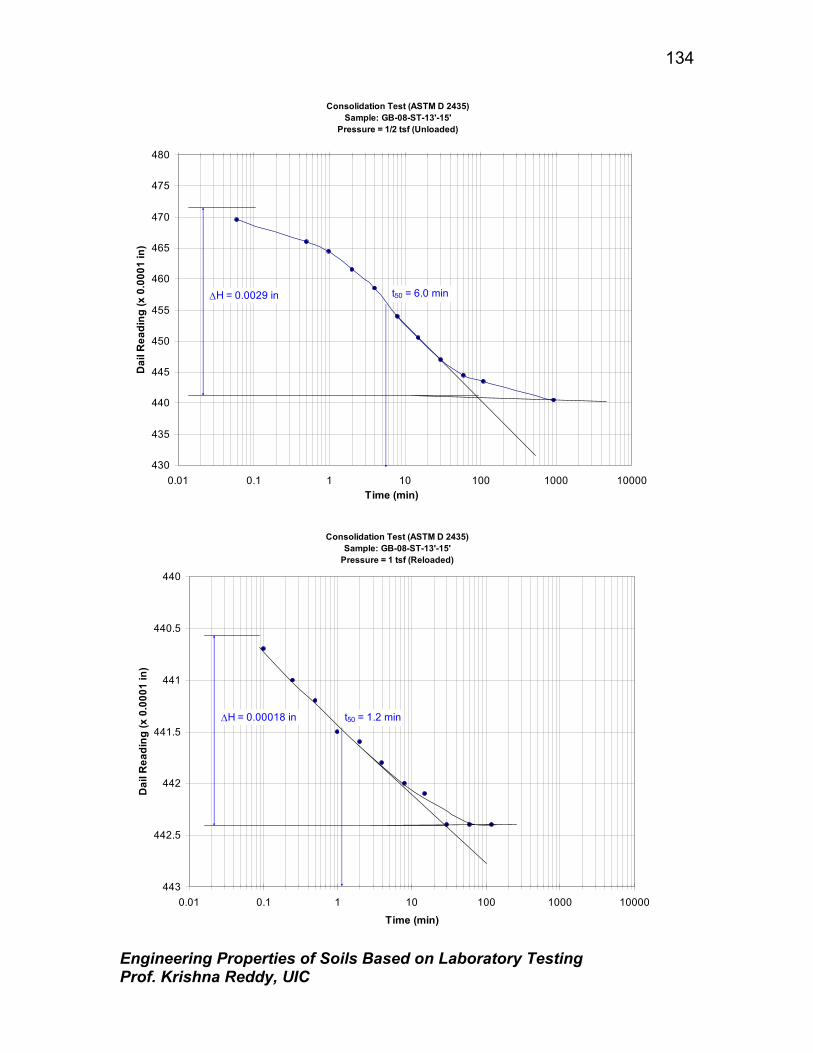
Engineering Properties of Soils Based on Laboratory Testing Prof. Krishna Reddy, UIC
134
Consolidation Test (ASTM D 2435)Sample: GB-08-ST-13'-15'
Pressure = 1/2 tsf (Unloaded)
430
435
440
445
450
455
460
465
470
475
480
0.01 0.1 1 10 100 1000 10000Time (min)
Dai
l Rea
ding
(x 0
.000
1 in
)
∆H = 0.0029 in t50 = 6.0 min
Consolidation Test (ASTM D 2435)
Sample: GB-08-ST-13'-15'Pressure = 1 tsf (Reloaded)
440
440.5
441
441.5
442
442.5
4430.01 0.1 1 10 100 1000 10000
Time (min)
Dai
l Rea
ding
(x 0
.000
1 in
)
t50 = 1.2 min∆H = 0.00018 in

Engineering Properties of Soils Based on Laboratory Testing Prof. Krishna Reddy, UIC
135
Consolidation Test (ASTM D 2435)Sample: GB-08-ST-13'-15'
Pressure = 2 tsf (Reloaded)
442
443
444
445
446
447
4480.01 0.1 1 10 100 1000 10000
Time (min)
Dai
l Rea
ding
(x 0
.000
1 in
)
∆H = 0.00038 int50 = 0.6 min
Consolidation Test (ASTM D 2435)
Sample: GB-08-ST-13'-15'Pressure = 4 tsf (Reloaded)
445
455
465
475
485
495
5050.01 0.1 1 10 100 1000 10000
Time (min)
Dai
l Rea
ding
(x 0
.000
1 in
)
t50 = 2.4 min∆H = 0.0043 in
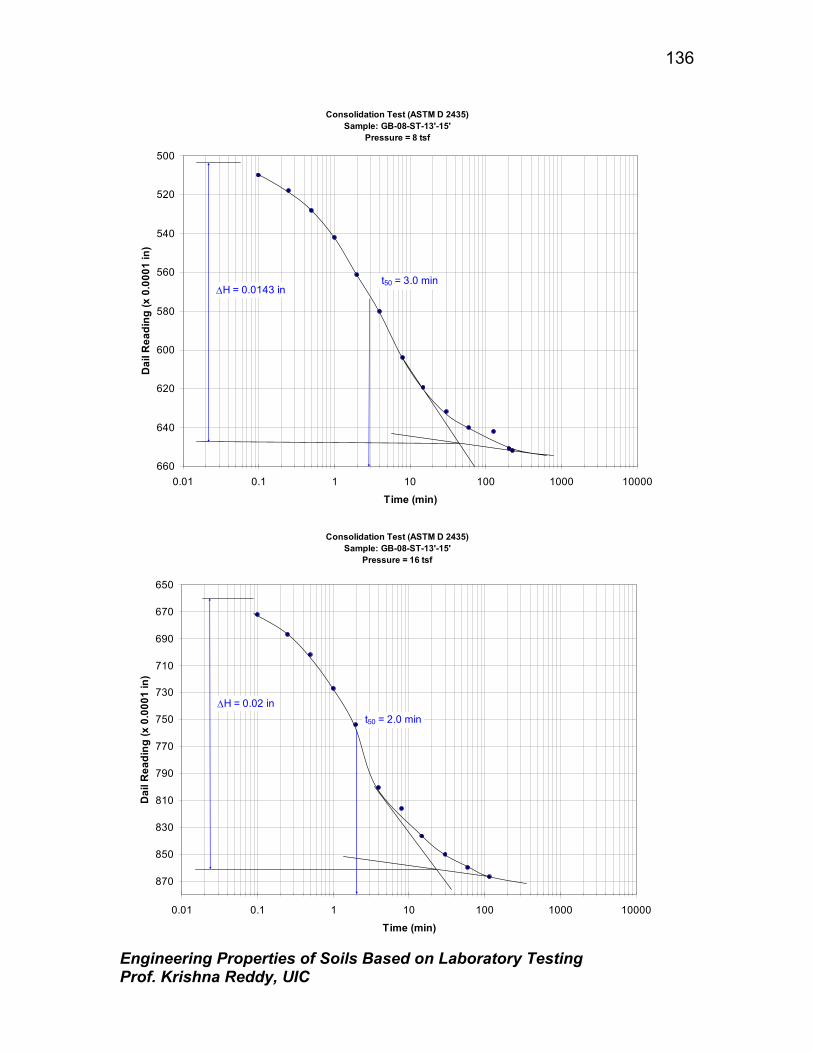
Engineering Properties of Soils Based on Laboratory Testing Prof. Krishna Reddy, UIC
136
Consolidation Test (ASTM D 2435)Sample: GB-08-ST-13'-15'
Pressure = 8 tsf
500
520
540
560
580
600
620
640
6600.01 0.1 1 10 100 1000 10000
Time (min)
Dai
l Rea
ding
(x 0
.000
1 in
)
t50 = 3.0 min∆H = 0.0143 in
Consolidation Test (ASTM D 2435)
Sample: GB-08-ST-13'-15'Pressure = 16 tsf
650
670
690
710
730
750
770
790
810
830
850
870
0.01 0.1 1 10 100 1000 10000
Time (min)
Dai
l Rea
ding
(x 0
.000
1 in
)
∆H = 0.02 int50 = 2.0 min

Engineering Properties of Soils Based on Laboratory Testing Prof. Krishna Reddy, UIC
137
Consolidation Test (ASTM D 2435)Sample: GB-08-ST-13'-15'
Pressure = 32 tsf
850
870
890
910
930
950
970
990
1010
1030
1050
1070
1090
0.01 0.1 1 10 100 1000 10000
Time (min)
Dai
l Rea
ding
(x 0
.000
1 in
)
t50 = 3.0 min
∆H = 0.0192 in

Engineering Properties of Soils Based on Laboratory Testing Prof. Krishna Reddy, UIC
138
Table 2: Analysis of Consolidation Test Data
Pressure (tsf)
Time for 50% consolidation
t 50 (min)
D0 (from
graph) D100 (from
graph)
D50 = (D0+D100)*0.5
Hj = D50 * 0.0001
∆H (from
graph) Σ ∆H* H** Hd
** Coefficient of consolidation
Cv (in2/min)*** Hv
*** e***
0 1.06299 0.5 10 8 159 83.5 0.00835 0.0153 0.0153 1.04769 0.52593 5.45E-03 0.34 0.481 11.5 173 254 213.5 0.02135 0.008 0.0233 1.03969 0.52518 4.72E-03 0.33 0.472 30 254 301 277.5 0.02775 0.0048 0.0281 1.03489 0.52438 1.81E-03 0.33 0.474 3.3 310 362 336 0.03360 0.0156 0.0437 1.01929 0.51805 1.60E-02 0.31 0.442 1.9 496 492.5 494.25 0.04943 0.0004 0.04335 1.01964 0.52218 2.83E-02 0.31 0.441 3.5 493 472.5 482.5 0.04825 0.002 0.04132 1.02167 0.52290 1.54E-02 0.32 0.45
0.5 6 472 442 457 0.04570 0.0029 0.03842 1.02457 0.52371 9.01E-03 0.32 0.451 1.2 441 442.4 441.5 0.04415 0.0002 0.0386 1.02439 0.52323 4.49E-02 0.32 0.452 0.6 443 446.5 444.55 0.04446 0.0004 0.03898 1.02401 0.52312 8.98E-02 0.32 0.454 2.4 446 489 467.5 0.04675 0.0043 0.04328 1.01971 0.52154 2.23E-02 0.31 0.448 3 504 650 577 0.05770 0.0143 0.05758 1.00541 0.51713 1.76E-02 0.30 0.42
16 2 660 861 760.5 0.07605 0.02 0.07758 0.98541 0.51172 2.58E-02 0.28 0.4032 3 869 1060 964.5 0.09645 0.0192 0.09678 0.96621 0.50722 1.69E-02 0.26 0.37
* Σ∆H for applied pressure = Σ∆H of all previous pressures + ∆H under applied pressure
** 1jHiHjHand4
jH
2
jH
jdH −∆±=∆
±= (- for Loading and + for Unloading)
***
50t
2dH
197.0vC ×= , ( ) HsHiHvH Σ∆−−= and sHvH
e =

Engineering Properties of Soils Based on Laboratory Testing Prof. Krishna Reddy, UIC
139
Consolidation Test (ASTM D 2435)Sample: GB-08-ST-13'-15'
Void Ratio vs Log Pressure
0.35
0.37
0.39
0.41
0.43
0.45
0.47
0.49
0.1 1 10 100Pressure (tsf)
Void
Rat
io
Cr=0.013
Cc=0.11
Pc=3.5 tsf
Final Results: Compression Index (Cc) = 0.11 Recompression Index (Cr) = 0.013 Preconsolidation pressure (Pc) or Maximum past pressure (σvmax) = 3.5 tsf Coefficient of consolidation (Cv)= 1.54x10⁻² to 9.01x10⁻³ in2/min (depends on the pressure) Coefficient of secondary compression (Cα) = 0.001 (It is the slope of time vs settlement curve beyond the end of primary consolidation)
Engineering Properties of Soils Based on Laboratory Testing Prof. Krishna Reddy, UIC
140
BLANK DATA SHEETS

Engineering Properties of Soils Based on Laboratory Testing Prof. Krishna Reddy, UIC
141
Consolidation Test Data Sheets
Date Tested: Tested By: Project Name: Sample Number: Sample Description: Before test Consolidation type = Mass of the ring + glass plate = Inside diameter of the ring = Height of specimen, Hi = Area of specimen, A = Mass of specimen + ring = Initial moisture content of specimen, wi (%) = Specific gravity of solids, Gs = After test Mass of wet sample + ring + glass plate = Mass of can = Mass of can + wet soil = Mass of wet specimen = Mass of can + dry soil = Mass of dry specimen, Ms = Final moisture content of specimen, wf =

Engineering Properties of Soils Based on Laboratory Testing Prof. Krishna Reddy, UIC
142
Calculations Mass of solids in specimen, Ms = (Mass of dry specimen after test) Mass of water in specimen before test, Mwi = wi x Ms= Mass of water in specimen after test, Mwf (g) = wf x Ms=
Height of solids, Hs = ws
s
GAM
ρ×× =
(same before and after test and note ρw = 1 g/cm3)
Height of water before test, Hwi = w
wi
AM
ρ× =
Height of water after test, Hwf = =× w
wf
AM
ρ=
Change in height of specimen after test, Σ∆H = (Σ∆H for all pressures – see t vs Dial reading plot) Height of specimen after test, Hf = Hi - Σ∆H =
Void ratio before test, eo = s
si
HHH − =
Void ratio after test, ef = s
sf
HHH −
=
Degree of saturation before test, Si = si
wi
HHH−
=
Degree of saturation after test, Sf = sf
wf
HH
H
−=
Dry density before test, ρd = AH
M
i
s
× =

Engineering Properties of Soils Based on Laboratory Testing Prof. Krishna Reddy, UIC
143
Time - Settlement Data Conversion: 0.0001 inch = 1.0 on dial reading (confirm this before using)
LOADING = _____ tsf ELAPSED TIME, min
DIAL READING
0 0.1 0.25 0.5 1 2 4 10 15 30 60 120 240
LOADING = _____ tsf ELAPSED TIME, min
DIAL READING
0 0.1 0.25 0.5 1 2 4 10 15 30 60 120 240
LOADING = _____ tsf ELAPSED TIME, min
DIAL READING
0 0.1 0.25 0.5 1 2 4 10 15 30 60 121 240

Engineering Properties of Soils Based on Laboratory Testing Prof. Krishna Reddy, UIC
144
Analysis of Consolidation Test Data
Pressure (tsf)
Time for 50% consolidation
t 50 (min)
D0 (from
graph) D100 (from
graph)
D50 = (D0+D100)*0.5
Hj = D50 * 0.0001
∆H (from
graph) Σ ∆H* H** Hd
** Coefficient of consolidation
Cv (in2/min) Hv
*** e***
* Σ∆H for applied pressure = Σ∆H of all previous pressures + ∆H under applied pressure
** 1jHiHjHand4
jH
2
jH
jdH −∆±=∆
±= (- for Loading and + for Unloading)
***
50t
2dH
197.0vC ×= , ( ) HsHiHvH Σ∆−−= and sHvH
e =

Engineering Properties of Soils Based on Laboratory Testing Prof. Krishna Reddy, UIC
145
EXPERIMENT 12
UNCONFINED COMPRESSION (UC) TEST
Purpose:
The primary purpose of this test is to determine the unconfined compressive
strength, which is then used to calculate the unconsolidated undrained shear
strength of the clay under unconfined condi tions. According to the ASTM standard,
the unconfined compressive strength (qu) is defined as the compressive stress at
which an unconfined cylindrical specimen of soil will fail in a simple compression
test. In addition, in this test method, the unconfined compressive strength is taken
as the maximum load attained per unit area, or the load per unit area at 15% axial
strain, whichever occurs first during the performance of a test.
Standard Reference:
ASTM D 2166 - Standard Test Method for Unconfined Compressive Strength
of Cohesive Soil
Significance:
For soils, the undrained shear strength (su) is necessary for the
determination of the bearing capacity of foundations, dams, etc. The undrained
shear strength (su) of clays is commonly determined from an unconfined
compression test. The undrained shear strength (su) of a cohesive soil is equal to
one-half the unconfined compressive strength (qu) when the soil is under the f = 0
condition (f = the angle of internal friction). The most critical condition for the soil
usually occurs immediately after construction, which represents undrained
conditions, when the undrained shear strength is basically equal to the cohesion
(c). This is expressed as:

Engineering Properties of Soils Based on Laboratory Testing Prof. Krishna Reddy, UIC
146
su = c = 2uq
Then, as time passes, the pore water in the soil slowly dissipates, and the
intergranular stress increases, so that the drained shear strength (s), given by s = c
+ s‘tan f , must be used. Where s‘ = intergranular pressure acting perpendicular to
the shear plane; and s‘ = (s - u), s = total pressure, and u = pore water pressure; c’
and ϕ’ are drained shear strength parameters. The determination of drained shear
strength parameters is given in Experiment 14
Equipment:
Compression device, Load and deformation dial gauges, Sample trimming
equipment, Balance, Moisture can.
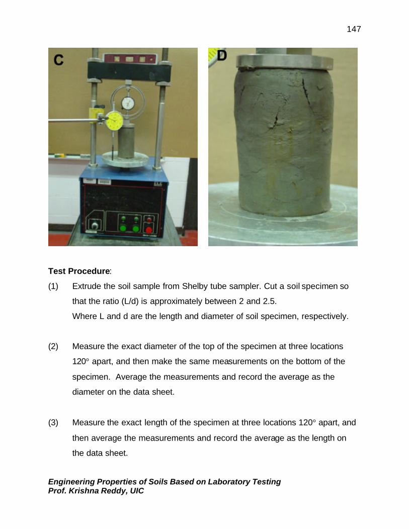
Engineering Properties of Soils Based on Laboratory Testing Prof. Krishna Reddy, UIC
147
Test Procedure:
(1) Extrude the soil sample from Shelby tube sampler. Cut a soil specimen so
that the ratio (L/d) is approximately between 2 and 2.5.
Where L and d are the length and diameter of soil specimen, respectively.
(2) Measure the exact diameter of the top of the specimen at three locations
120° apart, and then make the same measurements on the bottom of the
specimen. Average the measurements and record the average as the
diameter on the data sheet.
(3) Measure the exact length of the specimen at three locations 120° apart, and
then average the measurements and record the average as the length on
the data sheet.

Engineering Properties of Soils Based on Laboratory Testing Prof. Krishna Reddy, UIC
148
(4) Weigh the sample and record the mass on the data sheet.
(5) Calculate the deformation (∆L) corresponding to 15% strain (ε).
Strain (e) = oLL∆
Where L0 = Original specimen length (as measured in step 3).
(6) Carefully place the specimen in the compression device and center it on the
bottom plate. Adjust the device so that the upper plate just makes contact
with the specimen and set the load and deformation dials to zero.
(7) Apply the load so that the device produces an axial strain at a rate of 0.5% to
2.0% per minute, and then record the load and deformation dial readings on
the data sheet at every 20 to 50 divisions on deformation the dial.
(8) Keep applying the load until (1) the load (load dial) decreases on the
specimen significantly, (2) the load holds constant for at least four
deformation dial readings, or (3) the deformation is significantly past the 15%
strain that was determined in step 5.
(9) Draw a sketch to depict the sample failure.
(10) Remove the sample from the compression device and obtain a sample for
water content determination. Determine the water content as in Experiment
1.
Engineering Properties of Soils Based on Laboratory Testing Prof. Krishna Reddy, UIC
149
Analysis:
(1) Convert the dial readings to the appropriate load and length units, and enter
these values on the data sheet in the deformation and total load columns.
(Confirm that the conversion is done correctly, particularly proving dial gage
readings conversion into load)
(2) Compute the sample cross-sectional area ( )2d40A ×π
=
(3) Compute the strain, 0L
?Le =
(4) Computed the corrected area, e1
0A'A−
=
(5) Using A’, compute the specimen stress, s c = 'A
P
(Be careful with unit conversions and use constant units).
(6) Compute the water content, w%.
(7) Plot the stress versus strain. Show qu as the peak stress (or at 15% strain)
of the test. Be sure that the strain is plotted on the abscissa. See example
data.
(8) Draw Mohr’s circle using qu from the last step and show the undrained shear
strength, su = c (or cohesion) = qu/2. See the example data.
Engineering Properties of Soils Based on Laboratory Testing Prof. Krishna Reddy, UIC
150
EXAMPLE DATA
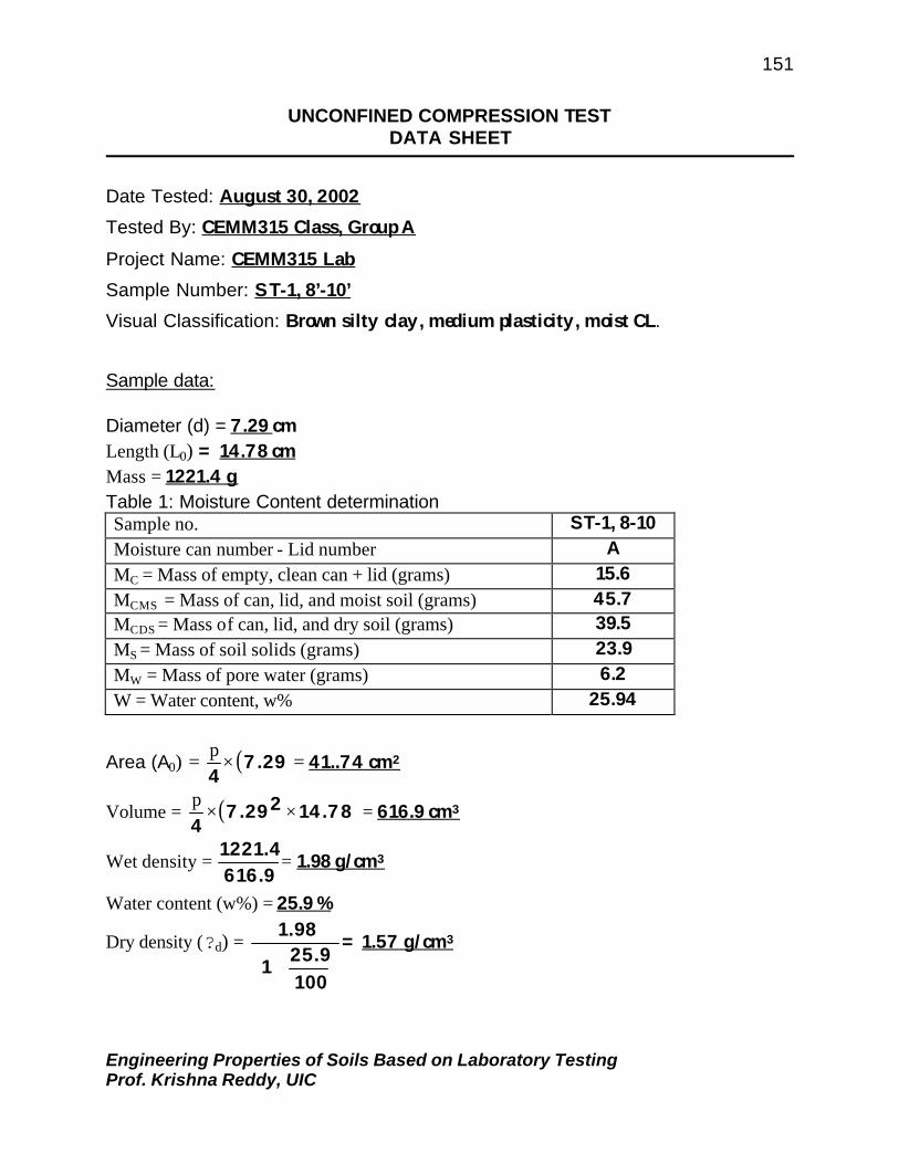
Engineering Properties of Soils Based on Laboratory Testing Prof. Krishna Reddy, UIC
151
UNCONFINED COMPRESSION TEST DATA SHEET
Date Tested: August 30, 2002
Tested By: CEMM315 Class, Group A Project Name: CEMM315 Lab Sample Number: ST-1, 8’-10’ Visual Classification: Brown silty clay, medium plasticity, moist CL.
Sample data: Diameter (d) = 7.29 cm Length (L0) = 14.78 cm Mass = 1221.4 g Table 1: Moisture Content determination Sample no. ST-1, 8-10 Moisture can number - Lid number A MC = Mass of empty, clean can + lid (grams) 15.6 MCMS = Mass of can, lid, and moist soil (grams) 45.7 MCDS = Mass of can, lid, and dry soil (grams) 39.5 MS = Mass of soil solids (grams) 23.9 MW = Mass of pore water (grams) 6.2 W = Water content, w% 25.94
Area (A0) = ( )7.294
×p
= 41..74 cm2
Volume = ( ) 14.7827.294
××p
= 616.9 cm3
Wet density = 616.91221.4
= 1.98 g/cm3
Water content (w%) = 25.9 %
Dry density (?d) =
+
10025.91
1.98 = 1.57 g/cm3

Engineering Properties of Soils Based on Laboratory Testing Prof. Krishna Reddy, UIC
152
Table 2: Unconfined Compression Test Data (Deformation Dial: 1 unit = 0.10mm; Proving Ring No: 24691; Load Dial: 1 unit = 0.3154 lb)
Deformation Dial Reading
Load Dial Reading
Sample Deformation
∆L (mm)
Strain (ε)
% Strain
Corrected Area A'
Load (lb)
Load (KN)
Stress (kPa)
0 0 0 0.000 0.000 41.739 0.000 0.000 0.000 20 4 0.2 0.001 0.135 41.796 1.262 56.131 1.343 40 9 0.4 0.003 0.271 41.853 2.839 126.295 3.018 60 12 0.6 0.004 0.406 41.909 3.785 168.393 4.018 80 19 0.8 0.005 0.541 41.966 5.994 266.622 6.353 100 21 1 0.007 0.677 42.024 6.625 294.687 7.012 120 24 1.2 0.008 0.812 42.081 7.571 336.786 8.003 140 26 1.4 0.009 0.947 42.138 8.202 364.851 8.658 160 29 1.6 0.011 1.083 42.196 9.148 406.949 9.644 180 33 1.8 0.012 1.218 42.254 10.410 463.080 10.959 200 36 2 0.014 1.353 42.312 11.356 505.178 11.939 250 45 2.5 0.017 1.691 42.457 14.196 631.473 14.873 300 54 3 0.020 2.030 42.604 17.035 757.768 17.786 350 64 3.5 0.024 2.368 42.752 20.189 898.095 21.007 400 74 4 0.027 2.706 42.900 23.344 1038.422 24.205 450 84 4.5 0.030 3.045 43.050 26.498 1178.750 27.381 500 93 5 0.034 3.383 43.201 29.338 1305.044 30.209 550 102 5.5 0.037 3.721 43.353 32.177 1431.339 33.016 600 112 6 0.041 4.060 43.505 35.331 1571.666 36.126 650 120 6.5 0.044 4.398 43.659 37.855 1683.928 38.570 700 129 7 0.047 4.736 43.814 40.694 1810.223 41.316 750 138 7.5 0.051 5.074 43.971 43.533 1936.517 44.041 800 144 8 0.054 5.413 44.128 45.426 2020.714 45.792 850 152 8.5 0.058 5.751 44.286 47.950 2132.976 48.163 900 160 9 0.061 6.089 44.446 50.473 2245.237 50.516 950 166 9.5 0.064 6.428 44.606 52.366 2329.434 52.222 1000 171 10 0.068 6.766 44.768 53.943 2399.598 53.600 1100 182 11 0.074 7.442 45.096 57.413 2553.958 56.634 1200 192 12 0.081 8.119 45.428 60.568 2694.285 59.309 1300 202 13 0.088 8.796 45.765 63.722 2834.612 61.939 1400 209 14 0.095 9.472 46.107 65.931 2932.841 63.610 1500 217 15 0.101 10.149 46.454 68.454 3045.103 65.551 1600 223 16 0.108 10.825 46.806 70.347 3129.300 66.856 1700 229 17 0.115 11.502 47.164 72.240 3213.496 68.134 1800 234 18 0.122 12.179 47.527 73.817 3283.660 69.090 1900 240 19 0.129 12.855 47.896 75.710 3367.856 70.315 2000 243 20 0.135 13.532 48.271 76.656 3409.954 70.642 2200 250 22 0.149 14.885 49.039 78.864 3508.184 71.539 2400 253 24 0.162 16.238 49.831 79.811 3550.282 71.247 2600 255 26 0.176 17.591 50.649 80.442 3578.347 70.650 2800 256 28 0.189 18.945 51.495 80.757 3592.380 69.762 3000 254 30 0.203 20.298 52.369 80.126 3564.314 68.062
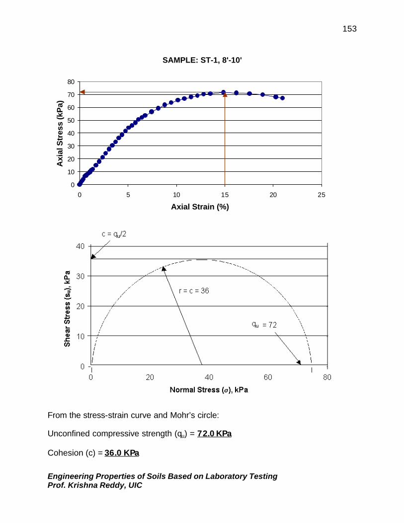
Engineering Properties of Soils Based on Laboratory Testing Prof. Krishna Reddy, UIC
153
SAMPLE: ST-1, 8'-10'
0
10
20
30
40
50
60
70
80
0 5 10 15 20 25
Axial Strain (%)
Axi
al S
tres
s (k
Pa)
From the stress-strain curve and Mohr’s circle:
Unconfined compressive strength (qu) = 72.0 KPa
Cohesion (c) = 36.0 KPa

Engineering Properties of Soils Based on Laboratory Testing Prof. Krishna Reddy, UIC
154
BLANK DATA SHEETS

Engineering Properties of Soils Based on Laboratory Testing Prof. Krishna Reddy, UIC
155
UNCONFINED COMPRESSION TEST DATA SHEET
Date Tested: Tested By: Project Name: Sample Number: Visual Classification:
Sample data: Diameter (d) = Length (L0) = Mass = Table 1: Moisture Content determination Sample no. Moisture can number - Lid number MC = Mass of empty, clean can + lid (grams) MCMS = Mass of can, lid, and moist soil (grams) MCDS = Mass of can, lid, and dry soil (grams) MS = Mass of soil solids (grams) MW = Mass of pore water (grams) W = Water content, w%
Area (A0) = Volume = Wet density = Water content (w%) = Dry density (?d) =

Engineering Properties of Soils Based on Laboratory Testing Prof. Krishna Reddy, UIC
156
Table 2: Unconfined Compression Test Data (Deformation Dial: 1 unit = 0.10mm; Proving Ring No: 24691; Load Dial: 1 unit = 0.3154 lb)
Deformation Dial Reading
Load Dial Reading
Sample Deformation
∆L (mm)
Strain (ε)
% Strain
Corrected Area A'
Load (lb)
Load (KN)
Stress (kPa)
0 20 40 60 80 100 120 140 160 180 200 250 300 350 400 450 500 550 600 650 700 750 800 850 900 950 1000 1100 1200 1300 1400 1500 1600 1700 1800 1900 2000 2200 2400 2600 2800 3000
Engineering Properties of Soils Based on Laboratory Testing Prof. Krishna Reddy, UIC
157
0
20
40
60
80
100
120
140
160
180
0 5 10 15 20 25
Axial Strain (%)
Axi
al S
tres
s (k
Pa)
0
10
20
30
40
50
60
70
80
90
100
0 10 20 30 40 50 60 70 80 90 100
Normal Stress (kPa)
Sh
ear
Str
ess
(kP
a)
From the stress-strain curve and Mohr’s circle:
Unconfined compressive strength (qu) =
Cohesion (c) =
Engineering Properties of Soils Based on Laboratory Testing Prof. Krishna Reddy, UIC
158
EXPERIMENT 13
DIRECT SHEAR TEST
Purpose:
This test is performed to determine the consolidated-drained shear strength
of a sandy to silty soil. The shear strength is one of the most important engineering
properties of a soil, because it is required whenever a structure is dependent on the
soil’s shearing resistance. The shear strength is needed for engineering situations
such as determining the stability of slopes or cuts, finding the bearing capacity for
foundations, and calculating the pressure exerted by a soil on a retaining wall.
Standard Reference:
ASTM D 3080 - Standard Test Method for Direct Shear Test of Soils Under
Consolidated Drained Conditions
Significance:
The direct shear test is one of the oldest strength tests for soils. In this
laboratory, a direct shear device will be used to determine the shear strength of a
cohesionless soil (i.e. angle of internal friction (f)). From the plot of the shear stress
versus the horizontal displacement, the maximum shear stress is obtained for a
specific vertical confining stress. After the experiment is run several times for
various vertical-confining stresses, a plot of the maxi mum shear stresses versus
the vertical (normal) confining stresses for each of the tests is produced. From the
plot, a straight-line approximation of the Mohr-Coulomb failure envelope curve can
be drawn, f may be determined, and, for cohesionless soils (c = 0), the shear
strength can be computed from the following equation:
tan fss =

Engineering Properties of Soils Based on Laboratory Testing Prof. Krishna Reddy, UIC
159
Equipment:
Direct shear device, Load and deformation dial gauges, Balance.

Engineering Properties of Soils Based on Laboratory Testing Prof. Krishna Reddy, UIC
160
Engineering Properties of Soils Based on Laboratory Testing Prof. Krishna Reddy, UIC
161
Test Procedure:
(1) Weigh the initial mass of soil in the pan.
(2) Measure the diameter and height of the shear box. Compute 15% of the
diameter in millimeters.
(3) Carefully assemble the shear box and place it in the direct shear device.
Then place a porous stone and a filter paper in the shear box.
(4) Place the sand into the shear box and level off the top. Place a filter paper, a
porous stone, and a top plate (with ball) on top of the sand
(5) Remove the large alignment screws from the shear box! Open the gap
between the shear box halves to approximately 0.025 in. using the gap
screws, and then back out the gap screws.
(6) Weigh the pan of soil again and compute the mass of soil used.
(7) Complete the assembly of the direct shear device and initialize the three
gauges (Horizontal displacement gage, vertical displacement gage and
shear load gage) to zero.
(8) Set the vertical load (or pressure) to a predetermined value, and then close
bleeder valve and apply the load to the soil specimen by raising the toggle
switch.
(9) Start the motor with selected speed so that the rate of shearing is at a
selected constant rate, and take the horizontal displacement gauge, vertical

Engineering Properties of Soils Based on Laboratory Testing Prof. Krishna Reddy, UIC
162
displacement gage and shear load gage readings. Record the readings on
the data sheet. (Note: Record the vertical displacement gage readings, if
needed).
(10) Continue taking readings until the horizontal shear load peaks and then falls,
or the horizontal displacement reaches 15% of the diameter.
Analysis:
(1) Calculate the density of the soil sample from the mass of soil and volume of
the shear box.
(2) Convert the dial readings to the appropriate length and load units and enter
the values on the data sheet in the correct locations. Compute the sample
area A, and the vertical (Normal) stress sv.
AN
s vv =
Where: Nv = normal vertical force, and sv = normal vertical stress
(3) Calculate shear stress (τ) using AhF
t =
Where Fh= shear stress (measured with shear load gage)
(4) Plot the horizontal shear stress (τ) versus horizontal (lateral) displacement
?H.
(5) Calculate the maximum shear stress for each test.

Engineering Properties of Soils Based on Laboratory Testing Prof. Krishna Reddy, UIC
163
(6) Plot the value of the maximum shear stress versus the corresponding
vertical stress for each test, and determine the angle of internal friction (f)
from the slope of the approximated Mohr-Coulomb failure envelope.

Engineering Properties of Soils Based on Laboratory Testing Prof. Krishna Reddy, UIC
164
DIRECT SHEAR TEST
DATA SHEET
Date Tested: August 30, 2002
Tested By: CEMM315 Class, Group A Project Name: CEMM315 Lab Sample Number: K-3,AU-10, 2’-4’ Visual Classification: Brown uniform sand Shear Box Inside Diameter: 6.3 cm Area (A): 31.17 cm2 = 4.83 in2 Shear Box Height: 4.9 cm Soil Volume: 119.9 cm3 Initial mass of soil and pan: 1000. g Final mass of soil and pan: 720.82 cm Mass of soil: 279.18 g Density of soil (?): 1.65 g/cm3

Engineering Properties of Soils Based on Laboratory Testing Prof. Krishna Reddy, UIC
165
Direct Shear Test Data
Displacement rate: _______ Normal stress: 2.27 psi
Horizontal Dial
Reading (0.001 in)
Horizontal Displacement
(in)
Load Dial Reading
Horizontal Shear Force
(lb)
Shear Stress (psi)
0 0 0 0 0 10 0.01 4 5.142 1.064 19 0.019 4.3 5.231 1.082 29 0.029 4.8 5.379 1.113 36 0.036 5 5.439 1.126 44 0.044 7 6.033 1.248 51 0.051 8 6.33 1.31 57 0.057 13.5 7.963 1.648 63 0.063 15 8.409 1.740 70 0.07 17 9.002 1.863 76 0.076 19 9.597 1.986 84 0.084 20 9.893 2.047 91 0.091 22 10.488 2.170
100 0.1 22.5 10.636 2.201 107 0.107 23 10.785 2.232 114 0.144 23.5 10.933 2.262
121.5 0.1215 25 11.379 2.355 129 0.129 25.5 11.527 2.385 137 0.137 26 11.675 2.416 145 0.145 27 11.973 2.478 152 0.152 27.5 12.121 2.508 160 0.16 28 12.270 2.539 179 0.179 25 11.379 2.355

Engineering Properties of Soils Based on Laboratory Testing Prof. Krishna Reddy, UIC
166
Direct Shear Test Data
Normal stress: 4.55 psi
Horizontal Dial Reading
(0.001 in)
Horizontal Displacement
(in)
Load Dial Reading
Horizontal Shear Force
(lb)
Shear Stress (psi)
0 0 0 0 0 4.5 0.0045 8 6.330 1.31 11 0.011 12 7.517 1.556 17 0.017 13.5 7.963 1.648 23 0.023 15.5 8.557 1.77 30 0.030 16.5 8.854 1.832 37 0.037 18.5 9.448 1.955 44 0.044 20 9.894 2.047 50 0.05 23 10.785 2.232 56 0.056 25.5 11.527 2.385 62 0.062 29 12.567 2.60 70 0.07 31.5 13.309 2.754 77 0.077 33 13.755 2.846 82 0.082 36 14.646 3.031 88 0.088 39 15.537 3.215 94 0.094 42 16.428 3.4 101 0.101 44 17.022 3.522 108 0.108 48 18.210 3.768 115 0.115 49 18.507 3.83 121 0.121 54 19.991 4.13 127 0.127 56.5 20.734 4.291 136 0.136 57.5 21.031 4.352 141 0.141 60 21.774 4.506 148 0.148 61.5 22.219 4.599 155 0.155 62 22.368 4.62

Engineering Properties of Soils Based on Laboratory Testing Prof. Krishna Reddy, UIC
167
Direct Shear Test Data
Normal stress: 6.82 psi
Horizontal Dial Reading
(0.001 in)
Horizontal Displacement
(in)
Load dial Reading
Horizontal Shear Force
(lb)
Shear Stress (psi)
0 0 0 0 0 1 0.001 16 8.706 1.801 5 0.005 22 10.488 2.170 10 0.01 27 11.972 2.478 15 0.015 31 13.16 2.723 21 0.021 34 14.052 2.908 28 0.028 36 14.646 3.031 34 0.034 41 16.131 3.338 39 0.039 41.5 16.279 3.37 42 0.042 43 16.725 3.461 51 0.051 45 17.319 3.584 61 0.061 47 17.913 3.707 68 0.068 50 18.804 3.891 74 0.074 54 19.99 4.13 82 0.082 56 20.586 4.26 88 0.088 58 21.18 4.383 94 0.094 61 22.071 4.568
101.5 0.1015 63 22.665 4.690 109 0.109 67 23.85 4.937 115 0.115 72 25.337 5.244 122 0.122 75 26.228 5.428 128 0.128 78 27.119 5.612 133 0.133 82 28.307 5.858 138 0.138 83 28.605 5.92 142 0.142 83 28.60 5.92

Engineering Properties of Soils Based on Laboratory Testing Prof. Krishna Reddy, UIC
168
0
1
2
3
4
5
6
7
0 0.02 0.04 0.06 0.08 0.1 0.12 0.14 0.16 0.18 0.2Horizontal Displacement (in)
Ho
rizo
nta
l Sh
ear
Str
ess
(psi
)
Normal Stress = 2.27 psi
Normal Stress = 4.55 psi
Normal Stress = 6.82 psi
2.6 psi
4.7 psi
5.9 psi
0
1
2
3
4
5
6
7
8
0 1 2 3 4 5 6 7 8
Normal Stress (psi)
Sh
ear
Str
ess
(psi
)
ϕ = 45ο

Engineering Properties of Soils Based on Laboratory Testing Prof. Krishna Reddy, UIC
169
BLANK DATA SHEETS

Engineering Properties of Soils Based on Laboratory Testing Prof. Krishna Reddy, UIC
170
DIRECT SHEAR TEST
DATA SHEET
Date Tested: Tested By: Project Name: Sample Number: Visual Classification: Shear Box Inside Diameter: Area (A): Shear Box Height: Soil Volume: Initial mass of soil and pan: Final mass of soil and pan: Mass of soil: Density of soil (?):

Engineering Properties of Soils Based on Laboratory Testing Prof. Krishna Reddy, UIC
171
Direct Shear Test Data
Displacement rate: _______ Normal stress: _______psi
Horizontal Dial Reading (0.001 in)
Horizontal Displacement
(in)
Load Dial Reading
Horizontal Shear Force
(lb)
Shear Stress (psi)

Engineering Properties of Soils Based on Laboratory Testing Prof. Krishna Reddy, UIC
172
Direct Shear Test Data Normal stress: _________ psi
Horizontal Dial Reading
(0.001 in)
Horizontal Displacement
(in)
Load Dial Reading
Horizontal Shear Force
(lb)
Shear Stress (psi)

Engineering Properties of Soils Based on Laboratory Testing Prof. Krishna Reddy, UIC
173
Direct Shear Test Data Normal stress: _______ psi
Horizontal Dial Reading
(0.001 in)
Horizontal Displacement
(in)
Load dial Reading
Horizontal Shear Force
(lb)
Shear Stress (psi)

Engineering Properties of Soils Based on Laboratory Testing Prof. Krishna Reddy, UIC
174
02468
1012141618202224262830
0 1 2 3 4 5 6 7 8 9 10Horizontal Displacement (in)
Ho
rizo
nta
l Sh
ear
Str
ess
(psi
)
0
2
4
6
8
10
12
14
16
18
20
0 2 4 6 8 10 12 14 16 18 20
Normal Stress (psi)
Sh
ear
Str
ess
(psi
)


