Soil Screening Guidance: Technical Background Document
447
United States Environmental Protection Agency Office of Solid Waste and Emergency Response Washington, DC 20460 EPA/540/R95/128 May 1996 Superfund Soil Screening Guidance: Technical Background Document Second Edition
Transcript of Soil Screening Guidance: Technical Background Document

United StatesEnvironmental Protection Agency
Office of Solid Waste andEmergency Response Washington, DC 20460
EPA/540/R95/128May 1996
Superfund
Soil Screening Guidance:Technical BackgroundDocument
Second Edition

Publication 9355.4-17AMay 1996
Soil Screening Guidance: Technical Background Document
Second Edition
Office of Emergency and Remedial ResponseU.S. Environmental Protection Agency
Washington, DC 20460

DISCLAIMER
Notice: The Soil Screening Guidance is based on policies set out in the Preamble to the Final Rule of the NationalOil and Hazardous Substances Pollution Contingency Plan (NCP), which was published on March 8, 1990 (55Federal Register 8666).
This guidance document sets forth recommended approaches based on EPA’s best thinking to date with respect tosoil screening. Alternative approaches for screening may be found to be more appropriate at specific sites (e.g.,where site circumstances do not match the underlying assumptions, conditions, and models of the guidance). Thedecision whether to use an alternative approach and a description of any such approach should be placed in theAdministrative Record for the site.
The policies set out in both the Soil Screening Guidance: User’s Guide and the supporting Soil ScreeningGuidance: Technical Background Document are intended solely as guidance to the U.S. Environmental ProtectionAgency (EPA) personnel; they are not final EPA actions and do not constitute rulemaking. These policies are notintended, nor can they be relied upon, to create any rights enforceable by any party in litigation with the UnitedStates government. EPA officials may decide to follow the guidance provided in this document, or to act at variancewith the guidance, based on an analysis of specific site circumstances. EPA also reserves the right to change theguidance at any time without public notice.
ii

TABLE OF CONTENTS
Section Page
Disclaimer . . . . . . . . . . . . . . . . . . . . . . . . . . . . . . . . . . . . . . . . . . . . . . . . . . . . . . . . . . . . . . iiList of Tables . . . . . . . . . . . . . . . . . . . . . . . . . . . . . . . . . . . . . . . . . . . . . . . . . . . . . . . . . . . . viList of Figures . . . . . . . . . . . . . . . . . . . . . . . . . . . . . . . . . . . . . . . . . . . . . . . . . . . . . . . . . . . viiiList of Highlights . . . . . . . . . . . . . . . . . . . . . . . . . . . . . . . . . . . . . . . . . . . . . . . . . . . . . . . . . viiiPreface . . . . . . . . . . . . . . . . . . . . . . . . . . . . . . . . . . . . . . . . . . . . . . . . . . . . . . . . . . . . . . . . . ixAcknowledgments . . . . . . . . . . . . . . . . . . . . . . . . . . . . . . . . . . . . . . . . . . . . . . . . . . . . . . . . . x
Part 1: Introduction1.1 Background . . . . . . . . . . . . . . . . . . . . . . . . . . . . . . . . . . . . . . . . . . . . . . . . . . . . . . . . . . . . 11.2 Purpose of SSLs . . . . . . . . . . . . . . . . . . . . . . . . . . . . . . . . . . . . . . . . . . . . . . . . . . . . . . . . . 21.3 Scope of Soil Screening Guidance . . . . . . . . . . . . . . . . . . . . . . . . . . . . . . . . . . . . . . . . . . . . . 3
1.3.1 Exposure Pathways . . . . . . . . . . . . . . . . . . . . . . . . . . . . . . . . . . . . . . . . . . . . . . . . . 41.3.2 Exposure Assumptions . . . . . . . . . . . . . . . . . . . . . . . . . . . . . . . . . . . . . . . . . . . . . . . 51.3.3 Risk Level . . . . . . . . . . . . . . . . . . . . . . . . . . . . . . . . . . . . . . . . . . . . . . . . . . . . . . . 51.3.4 SSL Model Assumptions . . . . . . . . . . . . . . . . . . . . . . . . . . . . . . . . . . . . . . . . . . . . . 6
1.4 Organization of the Document . . . . . . . . . . . . . . . . . . . . . . . . . . . . . . . . . . . . . . . . . . . . . . . . 6
Part 2: Development of Pathway-Specific Soil Screening Levels
2.1 Human Health Basis . . . . . . . . . . . . . . . . . . . . . . . . . . . . . . . . . . . . . . . . . . . . . . . . . . . . . . 92.1.1 Additive Risk . . . . . . . . . . . . . . . . . . . . . . . . . . . . . . . . . . . . . . . . . . . . . . . . . . . . . 92.1.2 Apportionment and Fractionation . . . . . . . . . . . . . . . . . . . . . . . . . . . . . . . . . . . . . . . 142.1.3 Acute Exposures . . . . . . . . . . . . . . . . . . . . . . . . . . . . . . . . . . . . . . . . . . . . . . . . . . 142.1.4 Route-to-Route Extrapolation . . . . . . . . . . . . . . . . . . . . . . . . . . . . . . . . . . . . . . . . . 16
2.2 Direct Ingestion . . . . . . . . . . . . . . . . . . . . . . . . . . . . . . . . . . . . . . . . . . . . . . . . . . . . . . . . 182.3 Dermal Absorption . . . . . . . . . . . . . . . . . . . . . . . . . . . . . . . . . . . . . . . . . . . . . . . . . . . . . . 202.4 Inhalation of Volatiles and Fugitive Dusts . . . . . . . . . . . . . . . . . . . . . . . . . . . . . . . . . . . . . . . 21
2.4.1 Screening Level Equations for Direct Inhalation . . . . . . . . . . . . . . . . . . . . . . . . . . . . . 212.4.2 Volatilization Factor . . . . . . . . . . . . . . . . . . . . . . . . . . . . . . . . . . . . . . . . . . . . . . . 232.4.3 Dispersion Model . . . . . . . . . . . . . . . . . . . . . . . . . . . . . . . . . . . . . . . . . . . . . . . . . 262.4.4 Soil Saturation Limit . . . . . . . . . . . . . . . . . . . . . . . . . . . . . . . . . . . . . . . . . . . . . . . 282.4.5 Particulate Emission Factor . . . . . . . . . . . . . . . . . . . . . . . . . . . . . . . . . . . . . . . . . . . 31
2.5 Migration to Ground Water . . . . . . . . . . . . . . . . . . . . . . . . . . . . . . . . . . . . . . . . . . . . . . . . . 322.5.1 Development of Soil/Water Partition Equation . . . . . . . . . . . . . . . . . . . . . . . . . . . . . . 342.5.2 Organic Compounds—Partition Theory . . . . . . . . . . . . . . . . . . . . . . . . . . . . . . . . . . 372.5.3 Inorganics (Metals)—Partition Theory . . . . . . . . . . . . . . . . . . . . . . . . . . . . . . . . . . . 402.5.4 Assumptions for Soil/Water Partition Theory . . . . . . . . . . . . . . . . . . . . . . . . . . . . . . . 402.5.5 Dilution/Attenuation Factor Development . . . . . . . . . . . . . . . . . . . . . . . . . . . . . . . . . 412.5.6 Default Dilution-Attenuation Factor . . . . . . . . . . . . . . . . . . . . . . . . . . . . . . . . . . . . . 462.5.7 Sensitivity Analysis . . . . . . . . . . . . . . . . . . . . . . . . . . . . . . . . . . . . . . . . . . . . . . . 54
2.6 Mass-Limit Model Development . . . . . . . . . . . . . . . . . . . . . . . . . . . . . . . . . . . . . . . . . . . . . 562.6.2 Migration to Ground Water Mass-Limit Model . . . . . . . . . . . . . . . . . . . . . . . . . . . . . 582.6.3 Inhalation Mass-Limit Model . . . . . . . . . . . . . . . . . . . . . . . . . . . . . . . . . . . . . . . . . 60
2.7 Plant Uptake . . . . . . . . . . . . . . . . . . . . . . . . . . . . . . . . . . . . . . . . . . . . . . . . . . . . . . . . . . 612.8 Intrusion of Volatiles into Basements: Johnson and Ettinger Model . . . . . . . . . . . . . . . . . . . . . . 62
iii

TABLE OF CONTENTS (continued)
Section Page
Part 3: Models for Detailed Assessment
3.1 Inhalation of Volatiles: Detailed Models . . . . . . . . . . . . . . . . . . . . . . . . . . . . . . . . . . . . . . . . 643.1.1 Finite Source Volatilization Models . . . . . . . . . . . . . . . . . . . . . . . . . . . . . . . . . . . . . 643.1.2 Air Dispersion Models . . . . . . . . . . . . . . . . . . . . . . . . . . . . . . . . . . . . . . . . . . . . . . 66
3.2 Migration to Ground Water Pathway . . . . . . . . . . . . . . . . . . . . . . . . . . . . . . . . . . . . . . . . . . 673.2.1 Saturated Zone Models . . . . . . . . . . . . . . . . . . . . . . . . . . . . . . . . . . . . . . . . . . . . . . 683.2.2 Unsaturated Zone Models . . . . . . . . . . . . . . . . . . . . . . . . . . . . . . . . . . . . . . . . . . . . 68
Part 4: Measuring Contaminant Concentrations in Soil
4.1 Sampling Surface Soils . . . . . . . . . . . . . . . . . . . . . . . . . . . . . . . . . . . . . . . . . . . . . . . . . . . 824.1.1 State the Problem . . . . . . . . . . . . . . . . . . . . . . . . . . . . . . . . . . . . . . . . . . . . . . . . . 824.1.2 Identify the Decision . . . . . . . . . . . . . . . . . . . . . . . . . . . . . . . . . . . . . . . . . . . . . . . 824.1.3 Identify Inputs to the Decision . . . . . . . . . . . . . . . . . . . . . . . . . . . . . . . . . . . . . . . . . 844.1.4 Define the Study Boundaries . . . . . . . . . . . . . . . . . . . . . . . . . . . . . . . . . . . . . . . . . . 844.1.5 Develop a Decision Rule . . . . . . . . . . . . . . . . . . . . . . . . . . . . . . . . . . . . . . . . . . . . 854.1.6 Specify Limits on Decision Errors for the Max Test . . . . . . . . . . . . . . . . . . . . . . . . . . . 864.1.7 Optimize the Design for the Max Test . . . . . . . . . . . . . . . . . . . . . . . . . . . . . . . . . . . . 874.1.8 Using the DQA Process: Analyzing Max Test Data . . . . . . . . . . . . . . . . . . . . . . . . . . . 964.1.9 Specify Limits on Decision Errors for Chen Test . . . . . . . . . . . . . . . . . . . . . . . . . . . . . 994.1.10 Optimize the Design Using the Chen Test . . . . . . . . . . . . . . . . . . . . . . . . . . . . . . . . . 1004.1.11 Using the DQA Process: Analyzing Chen Test Data . . . . . . . . . . . . . . . . . . . . . . . . . . 1074.1.12 Special Considerations for Multiple Contaminants . . . . . . . . . . . . . . . . . . . . . . . . . . . 1074.1.13 Quality Assurance/Quality Control Requirements . . . . . . . . . . . . . . . . . . . . . . . . . . . . 1074.1.14 Final Analysis . . . . . . . . . . . . . . . . . . . . . . . . . . . . . . . . . . . . . . . . . . . . . . . . . . . 1094.1.15 Reporting. . . . . . . . . . . . . . . . . . . . . . . . . . . . . . . . . . . . . . . . . . . . . . . . . . . . . . . 109
4.2 Sampling Subsurface Soils . . . . . . . . . . . . . . . . . . . . . . . . . . . . . . . . . . . . . . . . . . . . . . . . . 1104.2.1 State the Problem . . . . . . . . . . . . . . . . . . . . . . . . . . . . . . . . . . . . . . . . . . . . . . . . . 1104.2.2 Identify the Decision . . . . . . . . . . . . . . . . . . . . . . . . . . . . . . . . . . . . . . . . . . . . . . . 1104.2.3 Identify Inputs to the Decision . . . . . . . . . . . . . . . . . . . . . . . . . . . . . . . . . . . . . . . . . 1104.2.4 Define the Study Boundaries . . . . . . . . . . . . . . . . . . . . . . . . . . . . . . . . . . . . . . . . . . 1144.2.5 Develop a Decision Rule . . . . . . . . . . . . . . . . . . . . . . . . . . . . . . . . . . . . . . . . . . . . 1144.2.6 Specify Limits on Decision Errors . . . . . . . . . . . . . . . . . . . . . . . . . . . . . . . . . . . . . . 1144.2.7 Optimize the Design . . . . . . . . . . . . . . . . . . . . . . . . . . . . . . . . . . . . . . . . . . . . . . . 1154.2.8 Analyzing the Data . . . . . . . . . . . . . . . . . . . . . . . . . . . . . . . . . . . . . . . . . . . . . . . . 1164.2.9 Reporting . . . . . . . . . . . . . . . . . . . . . . . . . . . . . . . . . . . . . . . . . . . . . . . . . . . . . . 116
4.3 Basis for the Surface Soil Sampling Strategies: Technical Analyses Performed . . . . . . . . . . . . . . . 1174.3.1 1994 Draft Guidance Sampling Strategy . . . . . . . . . . . . . . . . . . . . . . . . . . . . . . . . . . 1174.3.2 Test of Proportion Exceeding a Threshold . . . . . . . . . . . . . . . . . . . . . . . . . . . . . . . . . 1194.3.3 Relative Performance of Land, Max, and Chen Tests . . . . . . . . . . . . . . . . . . . . . . . . . . 1214.3.4 Treatment of Observations Below the Limit of Quantitation . . . . . . . . . . . . . . . . . . . . . 1274.3.5 Multiple Hypothesis Testing Considerations . . . . . . . . . . . . . . . . . . . . . . . . . . . . . . . 1274.3.6 Investigation of Compositing Within EA Sectors . . . . . . . . . . . . . . . . . . . . . . . . . . . . 129
iv

TABLE OF CONTENTS (continued)
Section Page
Part 5: Chemical-Specific Parameters
5.1 Solubility, Henry's Law Constant, and Kow . . . . . . . . . . . . . . . . . . . . . . . . . . . . . . . . . . . . . . 1335.2 Air (Di,a) and Water (Di,w) Diffusivities . . . . . . . . . . . . . . . . . . . . . . . . . . . . . . . . . . . . . . . . . 1335.3 Soil Organic Carbon/Water Partition Coefficients (Koc) . . . . . . . . . . . . . . . . . . . . . . . . . . . . . . 139
5.3.1 Koc for Nonionizing Organic Compounds . . . . . . . . . . . . . . . . . . . . . . . . . . . . . . . . . 1395.3.2 Koc for Ionizing Organic Compounds . . . . . . . . . . . . . . . . . . . . . . . . . . . . . . . . . . . . 145
5.4 Soil-Water Distribution Coefficients (Kd) for Inorganic Constituents . . . . . . . . . . . . . . . . . . . . . . 1495.4.1 Modeling Scope and Approach . . . . . . . . . . . . . . . . . . . . . . . . . . . . . . . . . . . . . . . . 1525.4.2 Input Parameters . . . . . . . . . . . . . . . . . . . . . . . . . . . . . . . . . . . . . . . . . . . . . . . . . . 1535.4.3 Assumptions and Limitations . . . . . . . . . . . . . . . . . . . . . . . . . . . . . . . . . . . . . . . . . 1555.4.4 Results and Discussion . . . . . . . . . . . . . . . . . . . . . . . . . . . . . . . . . . . . . . . . . . . . . 1565.4.5 Analysis of Peer-Review Comments . . . . . . . . . . . . . . . . . . . . . . . . . . . . . . . . . . . . . 160
Part 6: References
References . . . . . . . . . . . . . . . . . . . . . . . . . . . . . . . . . . . . . . . . . . . . . . . . . . . . . . . . . . . . . . . . . . . . 161
Appendices
A Generic SSLs . . . . . . . . . . . . . . . . . . . . . . . . . . . . . . . . . . . . . . . . . . . . . . . . . . . . . . . . . . . A-1B Route-to-Route Extrapolation of Inhalation Benchmarks . . . . . . . . . . . . . . . . . . . . . . . . . . . . . . . B-1C Limited Validation of the Jury Infinite Source and Jury
Finite Source Models (EQ, 1995) . . . . . . . . . . . . . . . . . . . . . . . . . . . . . . . . . . . . . . . . . . . . . . C-1D Revisions to VF and PEF Equations (EQ, 1994b) . . . . . . . . . . . . . . . . . . . . . . . . . . . . . . . . . . . D-1E Determination of Ground Water Dilution Attenuation Factors . . . . . . . . . . . . . . . . . . . . . . . . . . . . E-1F Dilution Factor Modeling Results . . . . . . . . . . . . . . . . . . . . . . . . . . . . . . . . . . . . . . . . . . . . . . F-1G Background Discussion for Soil-Plant-Human Exposure Pathway . . . . . . . . . . . . . . . . . . . . . . . . . G-1H Evaluation of the Effect on the Draft SSLs of the Johnson and
Ettinger Model (EQ, 1994a) . . . . . . . . . . . . . . . . . . . . . . . . . . . . . . . . . . . . . . . . . . . . . . . . . . H-1I SSL Simulation Results . . . . . . . . . . . . . . . . . . . . . . . . . . . . . . . . . . . . . . . . . . . . . . . . . . . . I-1J Piazza Road Simulation Results . . . . . . . . . . . . . . . . . . . . . . . . . . . . . . . . . . . . . . . . . . . . . . . J-1K Soil Organic Carbon (Koc) / Water (Kow) Partition Coefficients . . . . . . . . . . . . . . . . . . . . . . . . . . K-1L Koc Values for Ionizing Organics as a Function of pH . . . . . . . . . . . . . . . . . . . . . . . . . . . . . . . . . L-1M Response to Peer-Review Comments on MINTEQA2 Model Results . . . . . . . . . . . . . . . . . . . . . M-1
v

LIST OF TABLES
Table 1. Regulatory and Human Health Benchmarks Used for SSL Development . . . . . . . . . . . . . . . . . . 10Table 2. SSL Chemicals with Noncarcinogenic Effects on Specific Target Organ/System . . . . . . . . . . . 15Table 3. Q/C Values by Source Area, City, and Climatic Zone . . . . . . . . . . . . . . . . . . . . . . . . . . . . 27Table 3-A. Risk Levels Calculated at Csat for Contaminants that have SSLinh Values
Greater than Csat . . . . . . . . . . . . . . . . . . . . . . . . . . . . . . . . . . . . . . . . . . . . . . . . . . . . . 29Table 4. Physical State of Organic SSL Chemicals . . . . . . . . . . . . . . . . . . . . . . . . . . . . . . . . . . . . 30Table 5. Variation of DAF with Size of Source Area for SSL EPACMTP Modeling Effort . . . . . . . . . . 48Table 6. Recharge Estimates for DNAPL Site Hydrogeologic Regions . . . . . . . . . . . . . . . . . . . . . . . . . 50Table 7. SSL Dilution Factor Model Results: DNAPL and HGDB Sites . . . . . . . . . . . . . . . . . . . . . . 51Table 8. Sensitivity Analysis for SSL Partition Equation . . . . . . . . . . . . . . . . . . . . . . . . . . . . . . . . . 53Table 9. Sensitivity Analysis for SSL Dilution Factor Model . . . . . . . . . . . . . . . . . . . . . . . . . . . . . 55Table 10. Input Parameters Required for RITZ Model . . . . . . . . . . . . . . . . . . . . . . . . . . . . . . . . . . . . . 67Table 11. Input Parameters Required for VIP Model . . . . . . . . . . . . . . . . . . . . . . . . . . . . . . . . . . . . . . 68Table 12. Input Parameters Required for CMLS . . . . . . . . . . . . . . . . . . . . . . . . . . . . . . . . . . . . . . . . . 69Table 13. Input Parameters Required for HYDRUS . . . . . . . . . . . . . . . . . . . . . . . . . . . . . . . . . . . . . . 70Table 14. Input Parameters Required for SUMMERS . . . . . . . . . . . . . . . . . . . . . . . . . . . . . . . . . . . . . 70Table 15. Input Parameters Required for MULTIMED . . . . . . . . . . . . . . . . . . . . . . . . . . . . . . . . . . . . 71Table 16. Input Parameters Required for VLEACH . . . . . . . . . . . . . . . . . . . . . . . . . . . . . . . . . . . . . . . 71Table 17. Input Parameters Required for SESOIL (Monthly Option) . . . . . . . . . . . . . . . . . . . . . . . . . . . 72Table 18. Input Parameters Required for PRZM . . . . . . . . . . . . . . . . . . . . . . . . . . . . . . . . . . . . . . . . . 74Table 19. Input Parameters Required for VADOFT . . . . . . . . . . . . . . . . . . . . . . . . . . . . . . . . . . . . . . 75Table 20. Characteristics of Unsaturated Zone Models Evaluated . . . . . . . . . . . . . . . . . . . . . . . . . . . . . . 76Table 21. Sampling Soil Screening DQOs for Surface Soils . . . . . . . . . . . . . . . . . . . . . . . . . . . . . . . . . 81Table 22. Sampling Soil Screening DQOs for Surface Soils under the Max Test . . . . . . . . . . . . . . . . . . . 86Table 23. Probability of Decision Error tat 0.5 SSL and 2 SSL Using Max Test . . . . . . . . . . . . . . . . . . . 93Table 24. Sampling Soil Screening DQOs for Surface Soils under Chen Test . . . . . . . . . . . . . . . . . . . . . 99Table 25. Minimum Sample Size for Chen Test at 10 Percent Level of Significance to
Achieve a 5 Percent Chance of “Walking Away” When EA Mean is 2.0 SSL, Given Expected CV for Concentrations Across the EA . . . . . . . . . . . . . . . . . . . . . . . . . . . . . 102
Table 26. Minimum Sample Size for Chen Test at 20 Percent Level of Significance to Achieve a 5 Percent Chance of “Walking Away” When EA Mean is 2.0 SSL, Given Expected CV for Concentrations Across the EA . . . . . . . . . . . . . . . . . . . . . . . . . . . . . 102
Table 27. Minimum Sample Size for Chen Test at 40 Percent Level of Significance to Achieve a 5 Percent Chance of “Walking Away” When EA Mean is 2.0 SSL, Given Expected CV for Concentrations Across the EA . . . . . . . . . . . . . . . . . . . . . . . . . . . . . 103
Table 28. Minimum Sample Size for Chen Test at 10 Percent Level of Significance to Achieve a 10 Percent Chance of “Walking Away” When EA Mean is 2.0 SSL, Given the Expected CV for Concentrations Across the EA . . . . . . . . . . . . . . . . . . . . . . . . . . . 103
Table 29. Minimum Sample Size for Chen Test at 20 Percent Level of Significance to Achieve a 10 Percent Chance of “Walking Away” When EA Mean is 2.0 SSL, Given Expected CV for Concentrations Across the EA . . . . . . . . . . . . . . . . . . . . . . . . . . . . . 104
Table 30. Minimum Sample Size for Chen Test at 40 Percent Level of Significance to Achieve a 10 Percent Chance of “Walking Away” When EA Mean is 2.0 SSL, Given Expected CV for Concentrations Across the EA . . . . . . . . . . . . . . . . . . . . . . . . . . . . . 104
Table 31. Soil Screening DQOs for Subsurface Soils . . . . . . . . . . . . . . . . . . . . . . . . . . . . . . . . . . . . . 109Table 32. Comparison of Error Rates for Max Test, Chen Test (at .20 and .10 Significance Levels),
and Original Land Test, Using 8 Composites of 6 Samples Each, for Gamma Contamination Data . . . . . . . . . . . . . . . . . . . . . . . . . . . . . . . . . . . . . . . . . . . . 123
vi

LIST OF TABLES (continued)
Table 33. Error Rates of Max Test and Chen Test at .2 (C20) and .1 (C10) Significance Level for CV = 2, 2.5, 3, 3.5, C = # of Specimens per Composite, N = # of Composite Samples . . . . . . . . . . . . . . . . . . . . . . . . . . . . . . . . . . . . . . . . . . . . . . 124
Table 34. Probability of "Walking Away" from an EA When Comparing Two Chemicals to SSLs . . . . . . . 127Table 35. Means and CVs for Dioxin Concentrations for 7 Piazza Road Exposure Areas . . . . . . . . . . . . . . 129Table 36. Chemical-Specific Properties Used in SSL Calculations . . . . . . . . . . . . . . . . . . . . . . . . . . . . 132Table 37. Air Diffusivity (Di,a) and Water Diffusivity (Di,w) Values for SSL Chemicals (25°C) . . . . . . . . . . 135Table 38. Summary Statistics for Measured Koc Values: Nonionizing Organics . . . . . . . . . . . . . . . . . . . . 139Table 39. Comparison of Measured and Calculated Koc Values . . . . . . . . . . . . . . . . . . . . . . . . . . . . . . . 141Table 40. Degree of Ionization (Fraction of Neutral Species, F) as a Function of pH . . . . . . . . . . . . . . . . . 145Table 41. Soil Organic Carbon/Water Partition Coefficients and pKa Values for Ionizing
Organic Compounds . . . . . . . . . . . . . . . . . . . . . . . . . . . . . . . . . . . . . . . . . . . . . . . . . . . . 147Table 42. Predicted Soil Organic Carbon/Water Partition Coefficients (Koc,L/kg) as a
Function of pH: Ionizing Organics . . . . . . . . . . . . . . . . . . . . . . . . . . . . . . . . . . . . . . . . . . . 148Table 43. Summary of Collected Kd Values Reported in Literature . . . . . . . . . . . . . . . . . . . . . . . . . . . . 149Table 44. Summary of Geochemical Parameters Used in SSL MINTEQ Modeling Effort . . . . . . . . . . . . . . 151Table 45. Background Pore-Water Chemistry Assumed for SSL MINTEQ Modeling Effort . . . . . . . . . . . . 152Table 46. Estimated Inorganic Kd Values for SSL Application . . . . . . . . . . . . . . . . . . . . . . . . . . . . . . . 154
vii

LIST OF FIGURES
Figure 1. Conceptual Risk Management Spectrum for Contaminated Soil . . . . . . . . . . . . . . . . . . . . . . . 2Figure 2. Exposure Pathways Addressed by SSLs. . . . . . . . . . . . . . . . . . . . . . . . . . . . . . . . . . . . . . . 4Figure 3. Migration to ground water pathway—EPACMTP modeling effort. . . . . . . . . . . . . . . . . . . . . . 46Figure 4. The Data Quality Objectives process. . . . . . . . . . . . . . . . . . . . . . . . . . . . . . . . . . . . . . . . . . 80Figure 5. Design performance goal diagram. . . . . . . . . . . . . . . . . . . . . . . . . . . . . . . . . . . . . . . . . . . . 87Figure 6. Systematic (square grid points) sample with systematic compositing scheme
(6 composite samples consisting of 4 specimens). . . . . . . . . . . . . . . . . . . . . . . . . . . . . . . . . 90Figure 7. Systematic (square grid points) sample with random compositing scheme
(6 composite samples consisting of 4 specimens). . . . . . . . . . . . . . . . . . . . . . . . . . . . . . . . . 91Figure 8. Stratified random sample with random compositing scheme
(6 composite samples consisting of 4 specimens). . . . . . . . . . . . . . . . . . . . . . . . . . . . . . . . . 92Figure 9. U.S. Department of Agriculture soil texture classification . . . . . . . . . . . . . . . . . . . . . . . . . . . . 112Figure 10. Empirical pH-dependent adsorption relationship: arsenic (+3),
chromium (+6), selenium, thallium . . . . . . . . . . . . . . . . . . . . . . . . . . . . . . . . . . . . . . . . . . 155Figure 11. Metal Kd as a function of pH. . . . . . . . . . . . . . . . . . . . . . . . . . . . . . . . . . . . . . . . . . . . . . . 156
LIST OF HIGHLIGHTS
Highlight 1: Key Attributes of the Soil Screening Guidance . . . . . . . . . . . . . . . . . . . . . . . . . . . . . . . . . . 3Highlight 2: Simplifying Assumptions for the Migration to Ground Water Pathway . . . . . . . . . . . . . . . . . 34Highlight 3: Procedure for Compositing of Specimens from a Grid Sample
Using a Systematic Scheme (Figure 6) . . . . . . . . . . . . . . . . . . . . . . . . . . . . . . . . . . . . . . 90Highlight 4: Procedure for Compositing of Specimens from a Grid Sample
Using a Random Scheme (Figure 7) . . . . . . . . . . . . . . . . . . . . . . . . . . . . . . . . . . . . . . . . 91Highlight 5: Procedure for Compositing of Specimens from a Stratified Random Sample
Using a Random Scheme (Figure 8) . . . . . . . . . . . . . . . . . . . . . . . . . . . . . . . . . . . . . . . . 92Highlight 6: Directions for Data Quality Assessment for the Max Test . . . . . . . . . . . . . . . . . . . . . . . . . . 96Highlight 7: Directions for the Chen Test Using Simple Random Sample Scheme . . . . . . . . . . . . . . . . . . 106
viii

PREFACE
This document provides the technical background for the development of methodologies described in the SoilScreening Guidance: User's Guide (EPA/540/R-96/018), along with additional information useful for soil screening.Together, these documents define the framework and methodology for developing Soil Screening Levels (SSLs) forchemicals commonly found at Superfund sites. This document is an updated version of the background documentdeveloped in support of the December 30, 1994, draft Soil Screening Guidance. The methodologies described in thisdocument and the guidance have been revised in response to public comment and extensive peer review. Therevisions, along with other technical analyses conducted to address the comments, are described herein.
This background document is presented in five parts. Part 1 describes the soil screening process and its applicationand implementation at Superfund sites. Part 2 describes the methodology used to develop SSLs, including theassumptions and theories used. Part 3 provides information on more detailed models that may be used to developsite-specific SSLs. Part 4 addresses sampling schemes for measuring soil contaminant levels during the soilscreening process. Part 5 provides technical background on the determination of chemical-specific properties forcalculating SSLs.
ix

ACKNOWLEDGMENTS
This technical background document was prepared by Research Triangle Institute (RTI) under EPA Contract 68-W1-0021, Work Assignment D2-24, for the Office of Emergency and Remedial Response (OERR), U.S.Environmental Protection Agency (EPA). Janine Dinan and Loren Henning of EPA, the EPA Work AssignmentManagers for this effort, guided the effort and are also principal EPA authors of the document along with Sherri Clarkof EPA. Robert Truesdale is the RTI Work Assignment Leader and principal RTI author of the document. CraigMann of Environmental Quality Management, Inc. (EQ), conducted the modeling effort for the inhalation pathwayand provided background information on that effort. Dr. Zubair Saleem of EPA's Office of Solid Waste conducted theEPACMTP modeling effort and provided the discussion on the use of this model for generic DAF development.The authors would like to thank all EPA, State, public, and peer reviewers whose careful review and thoughtfulcomments greatly contributed to the quality of this document. Technical support for the final document productionwas provided by Dr. Smita Siddhanti of Booz•Allen & Hamilton.
x

Part 1: INTRODUCTION
This document provides the technical background for the Soil Screening Guidance. The Soil ScreeningGuidance is a tool that the U.S. Environmental Protection Agency (EPA) developed to helpstandardize and accelerate the evaluation and cleanup of contaminated soils at sites on the NationalPriorities List (NPL) with anticipated future residential land use scenarios.1 This guidance provides amethodology for environmental science/engineering professionals to calculate risk-based, site-specific, soil screening levels (SSLs), for contaminants in soil that may be used to identify areasneeding further investigation at NPL sites.
SSLs are not national cleanup standards. SSLs alone do not trigger the need for responseactions or define "unacceptable" levels of contaminants in soil. "Screening," for the purposes of thisguidance, refers to the process of identifying and defining areas, contaminants, and conditions at aparticular site that do not require further Federal attention. Generally, at sites where contaminantconcentrations fall below SSLs, no further action or study is warranted under the ComprehensiveEnvironmental Response, Compensation, and Liability Act (CERCLA). (Some States have developedscreening numbers or methodologies that may be more stringent than SSLs; therefore further studymay be warranted under State programs.) Where contaminant concentrations equal or exceed theSSLs, further study or investigation, but not necessarily cleanup, is warranted.
The Soil Screening Guidance provides a framework for screening contaminated soils thatencompasses both simple and more detailed approaches for calculating site-specific SSLs, and genericSSLs for use where site-specific data are limited. The Soil Screening Guidance: User's Guide (U.S.EPA, 1996) focuses on the application of the simple site-specific approach by providing a step-by-step methodology to calculate site-specific SSLs and plan the sampling necessary to apply them.This Technical Background Document describes the development and technical basis of themethodology presented in the User’s Guide. It includes detailed modeling approaches for developingscreening levels that can take into account more complex site conditions than the simple site-specific methodology emphasized in the User's Guide. It also provides generic SSLs for the mostcommon contaminants found at NPL sites.
1 .1 Background
The Soil Screening Guidance is the result of technical analyses and coordination with numerousstakeholders. The effort began in 1991 when the EPA Administrator charged the Office of SolidWaste and Emergency Response (OSWER) with conducting a 30-day study to outline options foraccelerating the rate of cleanups at NPL sites. One of the specific proposals of the study was forOSWER to "examine the means to develop standards or guidelines for contaminated soils." Over thepast 4 years, several drafts of the guidance and the accompanying technical background documenthave had widespread reviews both within and outside EPA. In the Spring of 1995, final drafts werereleased for public comment and external scientific peer review. Many reviewers' commentscontributed significantly to the development of this flexible tool that uses site-specific data in amethodology that can be applied consistently across the nation.
1. Note that the Superfund program defines “soil” as having a particle size under 2 millimeters, while the RCRA programallows for particles under 9 millimeters in size.
1

1 .2 Purpose of SSLs
In identifying and managing risks at sites, EPA considers a spectrum of contaminant concentrations.The level of concern associated with those concentrations depends on the likelihood of exposure tosoil contamination at levels of potential concern to human health or to ecological receptors.Figure 1 illustrates the spectrum of soil contamination encountered at Superfund sites and theconceptual range of risk management. At one end are levels of contamination that clearly warrant aresponse action; at the other end are levels that are below regulatory concern. Appropriate cleanupgoals for a particular site may fall anywhere within this range depending on site-specific conditions.Screening levels identify the lower bound of the spectrum -- levels below which there is no concernunder CERCLA, provided conditions associated with the SSLs are met.
No further studywarranted under
CERCLA
Site-specificcleanup
goal/level
Response action clearly
warranted
"Zero"concentration
Screeninglevel
Responselevel
Very highconcentration
Figure 1. Conceptual Risk Management Spectrum forContaminated Soil
Although the application of SSLs during site investigations is not mandatory at sites being addressedby CERCLA or RCRA, EPA recommends the use of SSLs as a tool to facilitate prompt identificationof contaminants and exposure areas of concern. EPA developed the Soil Screening Guidance to beconsistent with and to enhance the current Superfund investigation process and anticipates itsprimary use during the early stages of a remedial investigation (RI) at NPL sites. It does not replacethe Remedial Investigation/Feasibility Study (RI/FS) or risk assessment, but use of screening levels canfocus the RI and risk assessment on aspects of the site that are more likely to be a concern underCERCLA. By screening out areas of sites, potential chemicals of concern, or exposure pathwaysfrom further investigation, site managers and technical experts can limit the scope of the remedialinvestigation or risk assessment. SSLs can save resources by helping to determine which areas do notrequire additional Federal attention early in the process. Furthermore, data gathered during the soilscreening process can be used in later Superfund phases, such as the baseline risk assessment,feasibility study, treatability study, and remedial design. This guidance may also be appropriate for useby the removal program when demarcation of soils above residential risk-based numbers coincideswith the purpose and scope of the removal action. EPA created the Soil Screening Guidance to beconsistent with and to enhance current Superfund processes.
The process presented in this guidance to develop and apply simple, site-specific soil screening levelsis likely to be most useful where it is difficult to determine whether areas of soil are contaminated toan extent that warrants further investigation or response (e.g., whether areas of soil at an NPL siterequire further investigation under CERCLA through an RI/FS). The screening levels have beendeveloped assuming future residential land use assumptions and related exposure scenarios. Althoughsome of the models and methods presented in this guidance could be modified to address exposures
2

under other land uses, EPA has not yet standardized assumptions for those other uses. Using thisguidance for sites where residential land use assumptions do not apply could result in overlyconservative screening levels. However, EPA recognizes that some parties responsible for sites withnon-residential land use might still benefit from using SSLs as a tool to conduct conservative initialscreening.
EPA created the Soil Screening Guidance: User’s Guide (U.S. EPA, 1996) to be easy to use: itprovides a simple step-by-step methodology for calculating SSLs that are specific to the user’s site.Applying site-specific screening levels involves developing a conceptual site model (CSM), collectinga few easily obtained site-specific soil parameters (such as the dry bulk density and percent soilmoisture), and sampling soil to measure contaminant levels in surface and subsurface soils. Often,much of the information needed to develop the CSM can be derived from previous site investigations(e.g., the preliminary assessment/site inspection [PA/SI]) and, if properly planned, SSL sampling canbe accomplished in one mobilization.
SSLs can be used as Preliminary Remediation Goals (PRGs) provided appropriate conditions are met(i.e., conditions found at a specific site are similar to conditions assumed in developing the SSLs).The concept of calculating risk-based soil levels for use as PRGs (or “draft” cleanup levels) wasintroduced in the Risk Assessment Guidance for Superfund (RAGS), Volume I, Human HealthEvaluation Manual (HHEM), Part B (U.S. EPA, 1991b). PRGs are risk-based values that provide areference point for establishing site-specific cleanup levels. The models, equations, and assumptionspresented in the Soil Screening Guidance and described herein to address inhalation exposuressupersede those described in RAGS HHEM, Part B, for residential soils. In addition, this guidancepresents methodologies to address the leaching of contaminants through soil to anunderlying potable aquifer. This pathway should be addressed in the development ofPRGs.
EPA emphasizes that SSLs are not cleanup standards. SSLs should not be used as site-specific cleanuplevels unless a site-specific nine-criteria evaluation using SSLs as PRGs for soils indicates that aselected remedy achieving the SSLs is protective, compliant with applicable or relevant andappropriate requirements (ARARs), and appropriately balances the other criteria, including cost.PRGs may then be converted into final cleanup levels based on the nine-criteria analysis described inthe National Contingency Plan (NCP; Section 300.430 (3)(2)(A)). The directive entitled Role of theBaseline Risk Assessment in Superfund Remedy Selection Decisions (U.S. EPA, 1991c) discusses themodification of PRGs to generate cleanup levels.
The generic SSLs provided in Appendix A are calculated from the same equations used in the simplesite-specific methodology, but are based on a number of default assumptions chosen to be protectiveof human health for most site conditions. Generic SSLs can be used in place of site-specific screeninglevels; however, they are expected to be generally more conservative than site-specific levels. Thesite manager should weigh the cost of collecting the data necessary to develop site-specific SSLs withthe potential for deriving a higher SSL that provides an appropriate level of protection.
1 .3 Scope of Soil Screening Guidance
The Soil Screening Guidance incorporates readily obtainable site data into simple, standardizedequations to derive site-specific screening levels for selected contaminants and exposure pathways.Key attributes of the Soil Screening Guidance are given in Highlight 1.
3

Highlight 1: Key Attributes of the Soil Screening Guidance
• Standardized equations are presented to address human exposure pathways in a residentialsetting consistent with Superfund's concept of "Reasonable Maximum Exposure" (RME).
• Source size (area and depth) can be considered on a site-specific basis using mass-limit models.
• Parameters are identified for which site-specific information is needed to develop site-specificSSLs.
• Default values are provided to calculate generic SSLs where site-specific information is notavailable.
• SSLs are generally based on a 10-6 risk for carcinogens, or a hazard quotient of 1 fornoncarcinogens; SSLs for migration to ground water are based on (in order of preference): nonzeromaximum contaminant level goals (MCLGs), maximum contaminant levels (MCLs), or theaforementioned risk-based targets.
1.3.1 Exposure Pathways. In a residential setting, potential pathways of exposure tocontaminants in soil are as follows (see Figure 2):
• Direct ingestion
• Inhalation of volatiles and fugitive dusts
• Ingestion of contaminated ground water caused by migration of chemicals through soil to anunderlying potable aquifer
• Dermal absorption
• Ingestion of homegrown produce that has been contaminated via plant uptake
• Migration of volatiles into Direct Ingestionof Ground
Water and Soil
Air
GroundWater
Leaching
Also Addressed:• Plant Uptake• Dermal Absorption
Inhalation
AAAAAAAAAAAAAAAAAAAAAAAAAAAAAAAAAAAAA
BlowingDust andVolatilizationDust and Volatization
Figure 2. Exposure Pathways Addressed by SSLs.
basements
The Soil Screening Guidance addresses each ofthese pathways to the greatest extent practical.The first three pathways -- direct ingestion,inhalation of volatiles and fugitive dusts, andingestion of potable ground water, are the mostcommon routes of human exposure tocontaminants in the residential setting. Thesepathways have generally accepted methods,models, and assumptions that lend themselves toa standardized approach. The additionalpathways of exposure to soil contaminants,dermal absorption, plant uptake, and migrationof volatiles into basements, may also contributeto the risk to human health from exposure tospecific contaminants in a residential setting.This guidance addresses these pathways to alimited extent based on available empirical data(see Part 2 for further discussion).
4
The Soil Screening Guidance addresses the human exposure pathways listed previouslyand will be appropriate for most residential settings. The presence of additional pathwaysor unusual site conditions does not preclude the use of SSLs in areas of the site that arecurrently residential or likely to be residential in the future. However, the risksassociated with these additional pathways or conditions (e.g., fish consumption, raising oflivestock, heavy truck traffic on unpaved roads) should be considered in the remedialinvestigation/feasibility study (RI/FS) to determine whether SSLs are adequatelyprotective.
An ecological assessment should also be performed as part of the RI/FS to evaluate poten-tial risks to ecological receptors.
The Soil Screening Guidance should not be used for areas with radioactive contaminants.
1.3.2 Exposure Assumptions. SSLs are risk-based concentrations derived from equationscombining exposure assumptions with EPA toxicity data. The models and assumptions used tocalculate SSLs were developed to be consistent with Superfund's concept of "reasonable maximumexposure" (RME) in the residential setting. The Superfund program's method to estimate the RMEfor chronic exposures on a site-specific basis is to combine an average exposure point concentrationwith reasonably conservative values for intake and duration in the exposure calculations (U.S. EPA,1989b; U.S. EPA, 1991a). The default intake and duration assumptions presented in U.S. EPA(1991a) were chosen to represent individuals living in a small town or other nontransientcommunity. (Exposure to members of a more transient community is assumed to be shorter and thusassociated with lower risk.) Exposure point concentrations are either measured at the site (e.g.,ground water concentrations at a receptor well) or estimated using exposure models with site-specificmodel inputs. An average concentration term is used in most assessments where the focus is onestimating long-term, chronic exposures. Where the potential for acute toxicity is of concern,exposure estimates based on maximum concentrations may be more appropriate.
The resulting site-specific estimate of RME is then compared with a chemical-specific toxicitycriterion such as a reference dose (RfD) or a reference concentration (RfC). EPA recommends usingcriteria from the Integrated Risk Information System (IRIS) (U.S. EPA, 1995b) and Health EffectsAssessment Summary Tables (HEAST) (U.S. EPA, 1995d), although values from other sources maybe used in appropriate cases.
SSLs are concentrations of contaminants in soil that are designed to be protective of exposures in aresidential setting. A site-specific risk assessment is an evaluation of the risk posed by exposure tosite contaminants in various media. To calculate SSLs, the exposure equations and pathway modelsare run in reverse to backcalculate an “acceptable level” of a contaminant in soil corresponding to aspecific level of risk.
1 . 3 . 3 Risk Level. For the ingestion, dermal, and inhalation pathways, toxicity criteria areused to define an acceptable level of contamination in soil, based on a one-in-a-million (10-6)individual excess cancer risk for carcinogens and a hazard quotient (HQ) of 1 for non-carcinogens.SSLs are backcalculated for migration to ground water pathways using ground water concentrationlimits [nonzero maximum contaminant level goals (MCLGs), maximum contaminant levels (MCLs),or health-based limits (HBLs) (10-6 cancer risk or a HQ of 1) where MCLs are not available].
The potential for additive effects has not been "built in" to the SSLs through apportionment. Forcarcinogens, EPA believes that setting a 10-6 risk level for individual chemicals and pathways willgenerally lead to cumulative risks within the risk range (10-4 to 10-6) for the combinations of
5
chemicals typically found at Superfund sites. For noncarcinogens, additive risks should be consideredonly for those chemicals with the same toxic endpoint or mechanism of action (see Section 2.1).
1.3.4 SSL Model Assumptions. The models used to calculate inhalation and migrationto ground water SSLs were designed for use at an early stage of site investigation when siteinformation may be limited. Because of this constraint, they incorporate a number of simplifyingassumptions.
The models assume that the source is infinite. Although the assumption is highly conservative, afinite source model cannot be applied unless there are accurate data regarding source size and volume.EPA believes it to be unlikely that such data will be available from the limited subsurface samplingthat is done to apply SSLs. However, EPA also recognizes that infinite source models can violatemass balance (i.e., can release more contaminants than are present) for certain contaminants and siteconditions (e.g., small sources). To address this problem, this guidance includes simple models thatprovide a mass-based limit for the inhalation and migration to ground water SSLs (see Section 2.6). Asite-specific estimate of source depth and area are required to calculate SSLs using thesemodels. The infinite source assumption leads to several other simplifying assumptions. Fractionation ofcontaminant mass between the inhalation and migration to ground water pathways cannot beaddressed with infinite source models. For the migration to ground water pathway, an infinite sourceoverrides adsorption in the unsaturated zone or in the aquifer. The models also assume thatcontamination is evenly distributed throughout the source (i.e., homogeneous) and that no biologicalor chemical degradation occurs in the soil or in the aquifer. Again, models capable of addressingheterogeneities or degradation processes require collection of site-specific data that is well beyond thescope of the Soil Screening Guidance.
Although the Soil Screening Guidance encourages the use of site-specific data to calculate SSLs,conservative default parameters are provided for use where site-specific data are not available. Thesedefaults are described in Part 2 of this document. Appendix A provides an example set of "generic"SSLs for 110 chemicals that are calculated using these defaults. Because they are designed to beprotective of most site conditions across the nation, they are conservative.
A default 0.5 acre source area is used to calculate the generic SSLs. A 30 acre source size was used inthe December 1994 guidance. EPA received an overwhelming number of comments that suggest thatmost contaminated soil sources addressed under the Superfund program are 0.5 acres or smaller.Because of the infinite source assumption, generic SSLs based on a 0.5 acre source size can beprotective of larger sources as well (see Appendix A). However, this hypothesis should be examinedon a case-by-case basis before applying the generic SSLs to sources larger than 0.5 acre.
1 .4 Organization of the Document
Part 2 of this document describes the development of the simple equations used to calculate SSLs. Itdescribes and supports the assumptions behind these equations and presents the results of analysesconducted to develop the SSL methodology. Some of the more sensitive parameters are identifiedfor which site-specific data are likely to have a significant impact. Default values are provided alongwith their sources and limitations.
Part 3 presents information on other, more complex models that can be used to calculate inhalationand migration to ground water SSLs when more extensive site data are available or can be obtained.
6

Some of these models can consider a finite source and fractionation between exposure pathways.They also can model more complex site conditions than the simple SSL equations, includingconditions that can lead to higher, yet still protective, SSLs (e.g., thick unsaturated zones, biologicaland chemical degradation, layered soils).
Part 4 provides the technical background for the development of the soil sampling designmethodology for SSL application. It addresses methods for surface soil, including a test based on amaximum soil composite sample and the Chen method, which allows decision errors to be controlled.Part 4 also provides simulation results that measure the performance of these methods and samplesize tables for different contaminant distributions and compositing schemes. Step-by-step guidance isprovided for developing sample designs using each statistical procedure.
Part 5 describes the selection and development of the chemical properties used to calculate SSLs.
7

1.1 Background . . . . . . . . . . . . . . . . . . . . . . . . . . . . . . . . . . . . . . . . . . . . . . . . . . . . . . . . . . . . 11.2 Purpose of SSLs . . . . . . . . . . . . . . . . . . . . . . . . . . . . . . . . . . . . . . . . . . . . . . . . . . . . . . . . . 21.3 Scope of Soil Screening Guidance . . . . . . . . . . . . . . . . . . . . . . . . . . . . . . . . . . . . . . . . . . . . . 3
1.3.1 Exposure Pathways . . . . . . . . . . . . . . . . . . . . . . . . . . . . . . . . . . . . . . . . . . . . . . . . . 41.3.2 Exposure Assumptions . . . . . . . . . . . . . . . . . . . . . . . . . . . . . . . . . . . . . . . . . . . . . . . 51.3.3 Risk Level . . . . . . . . . . . . . . . . . . . . . . . . . . . . . . . . . . . . . . . . . . . . . . . . . . . . . . . 51.3.4 SSL Model Assumptions . . . . . . . . . . . . . . . . . . . . . . . . . . . . . . . . . . . . . . . . . . . . . 6
1.4 Organization of the Document . . . . . . . . . . . . . . . . . . . . . . . . . . . . . . . . . . . . . . . . . . . . . . . . 6
8

Figure 1. Conceptual Risk Management Spectrum for Contaminated Soi . . . . . . . . . . . . . . . . . . . . . . . . . . 2 Figure 2. Exposure Pathways Addressed by SSLs. . . . . . . . . . . . . . . . . . . . . . . . . . . . . . . . . . . . . . . . . . . . . . . . . . . . . . . . . . . . . . . . . . . . . 4
9

Part 2: DEVELOPMENT OF PATHWAY-SPECIFIC SOIL SCREENING LEVELS
This part of the Technical Background Document describes the methods used to calculate SSLs forresidential exposure pathways, along with their technical basis and limitations associated with theiruse. Simple, standardized equations have been developed for three common exposure pathways atSuperfund sites:
• Ingestion of soil (Section 2.2)
• Inhalation of volatiles and fugitive dust (Section 2.4)
• Ingestion of contaminated ground water caused by migration of contaminants throughsoil to an underlying potable aquifer (Section 2.5).
The equations were developed under the following constraints:
• They should be consistent with current Superfund risk assessment methodologies andguidance.
• To be appropriate for early-stage application, they should be simple and easy toapply.
• They should allow the use of site-specific data where they are readily available or canbe easily obtained.
• The process of developing and applying SSLs should generate information that can beused and built upon as a site evaluation progresses.
The equations for the inhalation and migration to ground water pathways include easily obtained site-specific input parameters. Conservative default values have been developed for use where site-specificdata are not available. Generic SSLs, calculated for 110 chemicals using these default values, arepresented in Appendix A. The generic SSLs are conservative, since the default values are designed tobe protective at most sites across the country.
The inhalation and migration to ground water pathway equations assume an infinite source. Aspointed out by several commenters to the December 1994 draft Soil Screening Guidance (U.S. EPA,1994h), SSLs developed using these models may violate mass-balance for certain contaminants andsite conditions (e.g., small sources). To address this concern, EPA has incorporated simple mass-limitmodels for these pathways assuming that the entire volume of contamination either volatilizes orleaches over the duration of exposure and that the level of contaminant at the receptor does notexceed the health-based limit (Section 2.6). Because they require a site-specific estimate ofsource depth, these models cannot be used to calculate generic SSLs.
Dermal adsorption, consumption of garden vegetables grown in contaminated soil, and migration ofvolatiles into basements also may contribute significantly to the risk to human health from exposureto soil contaminants in a residential setting. These pathways have been incorporated into the SoilScreening Guidance to the greatest extent practical.
8

Although methods for quantifying dermal exposures are available, their use for calculating SSLs islimited by the amount of data available on dermal absorption of specific chemicals (Section 2.3).Screening equations have been developed to estimate human exposure from the uptake of soilcontaminants by garden plants (Section 2.7). As with dermal absorption, the number of chemicals forwhich adequate empirical data on plant uptake are limited. An approach to address migration ofvolatiles into basements is presented in Section 2.8, and limitations of the approach are discussed.
Section 2.1 describes the human health basis of the Soil Screening Guidance and provides the humantoxicity and health benchmarks necessary to calculate SSLs. The selection and development of thechemical properties required to calculate SSLs are described in Part 5 of this document.
2 .1 Human Health Basis
Table 1 lists the regulatory and human health benchmarks necessary to calculate SSLs for 110chemicals including:
• Ingestion SSLs: oral cancer slope factors (SFo) and noncancer reference doses (RfDs)
• Inhalation SSLs: inhalation unit risk factors (URFs) and reference concentrations(RfCs)
• Migration to ground water SSLs: drinking water standards (MCLGs and MCLs) anddrinking water health-based levels (HBLs).
The human health benchmarks in Table 1 were obtained from IRIS (U.S. EPA, 1995b) or HEAST(U.S. EPA, 1995d) unless otherwise indicated. MCLGs and MCLs were obtained from U.S. EPA(1995a). Each of these references is updated regularly. Prior to calculating SSLs, the values inTable 1 should be checked against the most recent version of these sources to ensure thatthey are up-to-date.
2.1.1 Additive Risk. For soil ingestion and inhalation of volatiles and fugitive dusts, SSLscorrespond to a 10-6 risk level for carcinogens and a hazard quotient of 1 for noncarcinogens. Forcarcinogens, EPA believes that setting a 10-6 risk level for individual chemicals and pathwaysgenerally will lead to cumulative risks within the 10-4 to 10-6 range for the combinations of chemicalstypically found at Superfund sites.
Whereas the carcinogenic risks of multiple chemicals are simply added together, the issue of additiverisk is much more complex for noncarcinogens because of the theory that a threshold exists fornoncancer effects. This threshold level, below which adverse effects are not expected to occur, is thebasis for EPA's RfD and RfC. Since adverse effects are not expected to occur at the RfD or RfC andthe SSLs were derived by setting the potential exposure dose equal to the RfD or RfC (i.e., an HQequal to 1), it is difficult to address the risk of exposure to multiple chemicals at levels where theindividual chemicals alone would not be expected to cause any harmful effect. However, problemsmay arise when multiple chemicals produce related toxic effects.
EPA believes, and the Science Advisory Board (SAB) agrees (U.S. EPA, 1993e), that HQs should beadded only for those chemicals with the same toxic endpoint and/or mechanism of action.
9

Table 1. Regulatory and Human Health Benchmarks Used for SSL Development
Maximum Contaminant Level
Goal(mg/L)
Maximum Contaminant Level
(mg/L)
Water Health Based Limits(mg/L)
Cancer Slope Factor(mg/kg-d)-1
Unit Risk Factor(µg/m3 )-1
Reference Dose(mg/kg-d)
Reference Concentration
(mg/m3 )
CASNumber Chemical Name MCLG
(PMCLG) Ref. a MCL (PMCL) Ref. a HBL b BasisCarc.
Class c SFo Ref. aCarc.
Class c URF Ref. a RfD Ref. a RfC Ref. a
83-32-9 Acenaphthene 2E+00 RfD 6.0E-02 167-64-1 Acetone (2-Propanone) 4E+00 RfD D D 1.0E-01 1
309-00-2 Aldrin 5E-06 SFo B2 1.7E+01 1 B2 4.9E-03 1 3.0E-05 1120-12-7 Anthracene 1E+01 RfD D D 3.0E-01 1
7440-36-0 Antimony 6.0E-03 3 6.0E-03 3 4.0E-04 17440-38-2 Arsenic 5.0E-02 3 A 1.5E+00 1 A 4.3E-03 1 3.0E-04 1
7440-39-3 Barium 2.0E+00 3 2.0E+00 3 7.0E-02 1 5.0E-04 2
56-55-3 Benz(a )anthracene 1E-04 SFo B2 7.3E-01 4 B2
71-43-2 Benzene 5.0E-03 3 A 2.9E-02 1 A 8.3E-06 1
205-99-2 Benzo(b )fluoranthene 1E-04 SFo B2 7.3E-01 4 B2
207-08-9 Benzo(k )fluoranthene 1E-03 SFo B2 7.3E-02 4 B2
65-85-0 Benzoic acid 1E+02 RfD 4.0E+00 1
50-32-8 Benzo(a )pyrene 2.0E-04 3 B2 7.3E+00 1 B2
7440-41-7 Beryllium 4.0E-03 3 4.0E-03 3 B2 4.3E+00 1 B2 2.4E-03 1 5.0E-03 1
111-44-4 Bis(2-chloroethyl)ether 8E-05 SFo B2 1.1E+00 1 B2 3.3E-04 1
117-81-7 Bis(2-ethylhexyl)phthalate 6.0E-03 3 B2 1.4E-02 1 B2 2.0E-02 1
75-27-4 Bromodichloromethane 1.0E-01 * 3 B2 6.2E-02 1 B2 2.0E-02 1
75-25-2 Bromoform (tribromomethane) 1.0E-01 * 3 B2 7.9E-03 1 B2 1.1E-06 1 2.0E-02 1
71-36-3 Butanol 4E+00 RfD D D 1.0E-01 1
85-68-7 Butyl benzyl phthalate 7E+00 RfD C C 2.0E-01 1
7440-43-9 Cadmium 5.0E-03 3 5.0E-03 3 B1 1.8E-03 1 1.0E-03** 1
86-74-8 Carbazole 4E-03 SFo B2 2.0E-02 2
75-15-0 Carbon disulfide 4E+00 RfD 1.0E-01 1 7.0E-01 1
56-23-5 Carbon tetrachloride 5.0E-03 3 B2 1.3E-01 1 B2 1.5E-05 1 7.0E-04 1
57-74-9 Chlordane 2.0E-03 3 B2 1.3E+00 1 B2 3.7E-04 1 6.0E-05 1
106-47-8 p -Chloroaniline 1E-01 RfD 4.0E-03 1
108-90-7 Chlorobenzene 1.0E-01 3 1.0E-01 3 D D 2.0E-02 1 2.0E-02 2
124-48-1 Chlorodibromomethane 6.0E-02 3 1.0E-01 * 3 C 8.4E-02 1 C 2.0E-02 1
67-66-3 Chloroform 1.0E-01 * 3 B2 6.1E-03 1 B2 2.3E-05 1 1.0E-02 1
95-57-8 2-Chlorophenol 2E-01 RfD 5.0E-03 1
* Proposed MCL = 0.08 mg/L, Drinking Water Regulations and Health Advisories , U.S. EPA (1995).
** Cadmium RfD is based on dietary exposure.
10

Table 1 (continued)
Maximum Contaminant Level
Goal(mg/L)
Maximum Contaminant Level
(mg/L)
Water Health Based Limits(mg/L)
Cancer Slope Factor(mg/kg-d)-1
Unit Risk Factor(µg/m3 )-1
Reference Dose(mg/kg-d)
Reference Concentration
(mg/m3 )
CASNumber Chemical Name MCLG
(PMCLG) Ref. a MCL (PMCL) Ref. a HBL b BasisCarc.
Class c SFo Ref. aCarc.
Class c URF Ref. a RfD Ref. a RfC Ref. a
7440-47-3 Chromium 1.0E-01 3 1.0E-01 3 A A 1.2E-02 1 5.0E-03 1
16065-83-1 Chromium (III) 4E+01 RfD 1.0E+00 1
18540-29-9 Chromium (VI) 1.0E-01 3 * A A 1.2E-02 1 5.0E-03 1
218-01-9 Chrysene 1E-02 SFo B2 7.3E-03 4
57-12-5 Cyanide (amenable) (2.0E-01) 3 (2.0E-01) 3 D D 2.0E-02 1
72-54-8 DDD 4E-04 SFo B2 2.4E-01 1 B2
72-55-9 DDE 3E-04 SFo B2 3.4E-01 1 B2
50-29-3 DDT 3E-04 SFo B2 3.4E-01 1 B2 9.7E-05 1 5.0E-04 1
53-70-3 Dibenz(a,h )anthracene 1E-05 SFo B2 7.3E+00 4 B2
84-74-2 Di-n -butyl phthalate 4E+00 RfD D D 1.0E-01 1
95-50-1 1,2-Dichlorobenzene 6.0E-01 3 6.0E-01 3 D D 9.0E-02 1 2.0E-01 2
106-46-7 1,4-Dichlorobenzene 7.5E-02 3 7.5E-02 3 B2 2.4E-02 2 B2 8.0E-01 1
91-94-1 3,3-Dichlorobenzidine 2E-04 SFo B2 4.5E-01 1 B2
75-34-3 1,1-Dichloroethane 4E+00 RfD C C 1.0E-01 7 5.0E-01 2
107-06-2 1,2-Dichloroethane 5.0E-03 3 B2 9.1E-02 1 B2 2.6E-05 1
75-35-4 1,1-Dichloroethylene 7.0E-03 3 7.0E-03 3 C 6.0E-01 1 C 5.0E-05 1 9.0E-03 1
156-59-2 cis -1,2-Dichloroethylene 7.0E-02 3 7.0E-02 3 D D 1.0E-02 2156-60-5 trans -1,2-Dichloroethylene 1.0E-01 3 1.0E-01 3 2.0E-02 1120-83-2 2,4-Dichlorophenol 1E-01 RfD 3.0E-03 1
78-87-5 1,2-Dichloropropane 5.0E-03 3 B2 6.8E-02 2 B2 4.0E-03 1
542-75-6 1,3-Dichloropropene 5E-04 SFo B2 1.8E-01 2 B2 3.7E-05 2 3.0E-04 1 2.0E-02 1
60-57-1 Dieldrin 5E-06 SFo B2 1.6E+01 1 B2 4.6E-03 1 5.0E-05 1
84-66-2 Diethylphthalate 3E+01 RfD D D 8.0E-01 1
105-67-9 2,4-Dimethylphenol 7E-01 RfD 2.0E-02 1
51-28-5 2,4-Dinitrophenol 4E-02 RfD 2.0E-03 1
121-14-2 2,4-Dinitrotoluene** 1E-04 SFo B2 6.8E-01 1 2.0E-03 1
606-20-2 2,6-Dinitrotoluene** 1E-04 SFo B2 6.8E-01 1 1.0E-03 2
117-84-0 Di-n -octyl phthalate 7E-01 RfD 2.0E-02 2
115-29-7 Endosulfan 2E-01 RfD 6.0E-03 2
72-20-8 Endrin 2.0E-03 3 2.0E-03 3 D D 3.0E-04 1
* MCL for total chromium is based on Cr (VI) toxicity.
** Cancer Slope Factor is for 2,4-, 2,6-Dinitrotoluene mixture.
11

Table 1 (continued)
Maximum Contaminant Level
Goal(mg/L)
Maximum Contaminant Level
(mg/L)
Water Health Based Limits(mg/L)
Cancer Slope Factor(mg/kg-d)-1
Unit Risk Factor(µg/m3 )-1
Reference Dose(mg/kg-d)
Reference Concentration
(mg/m3 )
CASNumber Chemical Name MCLG
(PMCLG) Ref. a MCL (PMCL) Ref. a HBL b BasisCarc.
Class c SFo Ref. aCarc.
Class c URF Ref. a RfD Ref. a RfC Ref. a
100-41-4 Ethylbenzene 7.0E-01 3 7.0E-01 3 D D 1.0E-01 1 1.0E+00 1
206-44-0 Fluoranthene 1E+00 RfD D D 4.0E-02 1
86-73-7 Fluorene 1E+00 RfD D 4.0E-02 1
76-44-8 Heptachlor 4.0E-04 3 B2 4.5E+00 1 B2 1.3E-03 1 5.0E-04 1
1024-57-3 Heptachlor epoxide 2.0E-04 3 B2 9.1E+00 1 B2 2.6E-03 1 1.3E-05 1
118-74-1 Hexachlorobenzene 1.0E-03 3 B2 1.6E+00 1 B2 4.6E-04 1 8.0E-04 1
87-68-3 Hexachloro-1,3-butadiene 1.0E-03 3 1E-03 SFo C 7.8E-02 1 C 2.2E-05 1 2.0E-04 2319-84-6 α-HCH (α-BHC) 1E-05 SFo B2 6.3E+00 1 B2 1.8E-03 1319-85-7 β-HCH (β-BHC) 5E-05 SFo C 1.8E+00 1 C 5.3E-04 1
58-89-9 γ-HCH (Lindane) 2.0E-04 3 2.0E-04 3 B2 1.3E+00 2 C 3.0E-04 1
77-47-4 Hexachlorocyclopentadiene 5.0E-02 3 5.0E-02 3 D D 7.0E-03 1 7.0E-05 2
67-72-1 Hexachloroethane 6E-03 SFo C 1.4E-02 1 C 4.0E-06 1 1.0E-03 1
193-39-5 Indeno(1,2,3-cd )pyrene 1E-04 SFo B2 7.3E-01 4 B2
78-59-1 Isophorone 9E-02 SFo C 9.5E-04 1 C 2.0E-01 1
7439-97-6 Mercury 2.0E-03 3 2.0E-03 3 D D 3.0E-04 2 3.0E-04 2
72-43-5 Methoxychlor 4.0E-02 3 4.0E-02 3 D D 5.0E-03 1
74-83-9 Methyl bromide 5E-02 RfD D D 1.4E-03 1 5.0E-03 1
75-09-2 Methylene chloride 5.0E-03 3 B2 7.5E-03 1 B2 4.7E-07 1 6.0E-02 1 3.0E+00 2
95-48-7 2-Methylphenol (o -cresol) 2E+00 RfD C C 5.0E-02 1
91-20-3 Naphthalene 1E+00 RfD D D 4.0E-02 6
7440-02-0 Nickel 1E-01 HA * A A 2.4E-04 1 2.0E-02 1
98-95-3 Nitrobenzene 2E-02 RfD D D 5.0E-04 1 2.0E-03 2
86-30-6 N -Nitrosodiphenylamine 2E-02 SFo B2 4.9E-03 1 B2
621-64-7 N -Nitrosodi-n -propylamine 1E-05 SFo B2 7.0E+00 1 B287-86-5 Pentachlorophenol 1.0E-03 3 B2 1.2E-01 1 B2 3.0E-02 1
108-95-2 Phenol 2E+01 RfD D D 6.0E-01 1129-00-0 Pyrene 1E+00 RfD D D 3.0E-02 1
7782-49-2 Selenium 5.0E-02 3 5.0E-02 3 D D 5.0E-03 17440-22-4 Silver 2E-01 RfD D D 5.0E-03 1100-42-5 Styrene 1.0E-01 3 1.0E-01 3 2.0E-01 1 1.0E+00 1
79-34-5 1,1,2,2-Tetrachloroethane 4E-04 SFo C 2.0E-01 1 C 5.8E-05 1
* Health advisory for nickel (MCL is currently remanded); EPA Office of Science and Technology, 7/10/95.
12

Table 1 (continued)
Maximum Contaminant Level
Goal(mg/L)
Maximum Contaminant Level
(mg/L)
Water Health Based Limits(mg/L)
Cancer Slope Factor(mg/kg-d)-1
Unit Risk Factor(µg/m3 )-1
Reference Dose(mg/kg-d)
Reference Concentration
(mg/m3 )
CASNumber Chemical Name MCLG
(PMCLG) Ref. a MCL (PMCL) Ref. a HBL b BasisCarc.
Class c SFo Ref. aCarc.
Class c URF Ref. a RfD Ref. a RfC Ref. a
127-18-4 Tetrachloroethylene 5.0E-03 3 5.2E-02 5 5.8E-07 5 1.0E-02 17440-28-0 Thallium 5.0E-04 3 2.0E-03 3108-88-3 Toluene 1.0E+00 3 1.0E+00 3 D D 2.0E-01 1 4.0E-01 1
8001-35-2 Toxaphene 3.0E-03 3 B2 1.1E+00 1 B2 3.2E-04 1120-82-1 1,2,4-Trichlorobenzene 7.0E-02 3 7.0E-02 3 D D 1.0E-02 1 2.0E-01 2
71-55-6 1,1,1-Trichloroethane 2.0E-01 3 2.0E-01 3 D D 1.0E+00 5
79-00-5 1,1,2-Trichloroethane 3.0E-03 3 5.0E-03 3 C 5.7E-02 1 C 1.6E-05 1 4.0E-03 179-01-6 Trichloroethylene zero 3 5.0E-03 3 1.1E-02 5 1.7E-06 595-95-4 2,4,5-Trichlorophenol 4E+00 RfD 1.0E-01 1
88-06-2 2,4,6-Trichlorophenol 8E-03 SFo B2 1.1E-02 1 B2 3.1E-06 17440-62-2 Vanadium 3E-01 RfD 7.0E-03 2108-05-4 Vinyl acetate 4E+01 RfD 1.0E+00 1 2.0E-01 1
75-01-4 Vinyl chloride (chloroethene) 2.0E-03 3 A 1.9E+00 2 A 8.4E-05 2
108-38-3 m -Xylene 1.0E+01 3 * 1.0E+01 3 * D D 2.0E+00 2
95-47-6 o -Xylene 1.0E+01 3 * 1.0E+01 3 * D D 2.0E+00 2
106-42-3 p -Xylene 1.0E+01 3 * 1.0E+01 3 * D D 2.0E+00 1 **
7440-66-6 Zinc 1E+01 RfD D D 3.0E-01 1
* MCL for total xylenes [1330-20-7] is 10 mg/L.
** RfD for total xylenes is 2 mg/kg-day.
a References: 1 = IRIS, U.S. EPA (1995b) c Categorization of overall weight of evidence for human carcinogenicity:
2 = HEAST, U.S. EPA (1995d) Group A: human carcinogen
3 = U.S. EPA (1995a) Group B: probable human carcinogen
4 = OHEA, U.S. EPA (1993c) B1: limited evidence from epidemiologic studies
5 = Interim toxicity criteria provided by Superfund B2: "sufficient" evidence from animal studies and "inadequate" evidence or
Health Risk Techincal Support Center, "no data" from epidemiologic studies
Environmental Criteria Assessment Office Group C: possible human carcinogen
(ECAO), Cincinnati, OH (1994) Group D: not classifiable as to health carcinogenicity
6 = ECAO, U.S. EPA (1994g) Group E: evidence of noncarcinogenicity for humans
7 = ECAO, U.S. EPA (1994f)b Health Based Limits calculated for 30-year exposure duration, 10-6 risk or hazard quotient = 1.
13

Additivity of the SSLs for noncarcinogenic chemicals is further complicated by the fact that not allSSLs are based on toxicity. Some SSLs are determined instead by a "ceiling limit" concentration (C sat)above which these chemicals may occur as nonaqueous phase liquids (NAPLs) in soil (see Section2.4.4). Therefore, the potential for additive effects must be carefully evaluated at every site byconsidering the total Hazard Index (HI) for chemicals with RfDs or RfCs based on the same endpointof toxicity (i.e., has the same critical effect as defined by the Reference Dose Methodology),excluding chemicals with SSLs based on Csat. Table 2 lists several SSL chemicals with RfDs/RfCs,grouping those chemicals whose RfDs or RfCs are based on toxic effects in the same target organ orsystem. However, this list is limited, and a toxicologist should be consulted prior to addressingadditive risks at a specific site.
2.1.2 Apportionment and Fractionation. EPA also has evaluated the SSLs fornoncarcinogens in light of two related issues: apportionment and fractionation. Apportionment istypically used as the percentage of a regulatory health-based level that is allocated to thesource/pathway being regulated (e.g., 20 percent of the RfD for the migration to ground waterpathway). Apportioning risk assumes that the applied dose from the source, in this casecontaminated soils, is only one portion of the total applied dose received by the receptor. In theSuperfund program, EPA has traditionally focused on quantifying exposures to a receptor that areclearly site-related and has not included exposures from other sources such as commercially availablehousehold products or workplace exposures. Depending on the assumptions concerning other sourcecontributions, apportionment among pathways and sources at a site may result in moreconservative regulatory levels (e.g., levels that are below an HQ of 1). Depending on site conditions,this may be appropriate on a site-specific basis.
In contrast to apportionment, fractionation of risk may lead to less conservative regulatorylevels because it assumes that some fraction of the contaminant does not reach the receptor due topartitioning into another medium. For example, if only one-fifth of the source is assumed to beavailable to the ground water pathway, and the remaining four-fifths is assumed to be released to airor remain in the soil, an SSL for the migration to ground water pathway could be set at five times theHQ of 1 due to the decrease in exposure (since only one-fifth of the possible contaminant is availableto the pathway). However, the data collected to apply SSLs generally will not support the finitesource models necessary for partitioning contaminants between pathways.
2.1.3 Acute Exposures. The exposure assumptions used to develop SSLs are representativeof a chronic exposure scenario and do not account for situations where high-level exposures may leadto acute toxicity. For example, in some cases, children may ingest large amounts of soil (e.g., 3 to 5grams) in a single event. This behavior, known as pica, may result in relatively high short-termexposures to contaminants in soils. Such exposures may be of concern for contaminants thatprimarily exhibit acute health effects. Review of clinical reports on contaminants addressed in thisguidance suggests that acute effects of cyanide and phenol may be of concern in children exhibitingpica behavior. If soils containing cyanide and phenol are present at a site, the protectiveness of thechronic ingestion SSLs for these chemicals should be reconsidered.
Although the Soil Screening Guidance instructs site managers to consider the potential for acuteexposures on a site-specific basis, there are two major impediments to developing acute SSLs. First,although data are available on chronic exposures (i.e., RfDs, RfCs, cancer slope factors), there is apaucity of data relating the potential for acute effects for most Superfund chemicals. Specifically,there is no scale to evaluate the severity of acute effects (e.g., eye irritation vs. dermatitis), noconsensus on how to incorporate the body's recovery mechanisms following acute exposures, and notoxicity benchmarks to apply for short-term exposures (e.g., a 7-day RfD for a critical endpoint).
14

Table 2. SSL Chemicals with Noncarcinogenic Effects on Specific TargetOrgan/System
Target Organ/System Ef fec t
KidneyAcetone Increased weight; nephrotoxicity1,1-Dichloroethane Kidney damageCadmium Significant proteinuriaChlorobenzene Kidney effectsDi-n-octyl phthalate Kidney effects
Endosulfan GlomerulonephrosisEthylbenzene Kidney toxicityFluoranthene NephropathyNitrobenzene Renal and adrenal lesionsPyrene Kidney effectsToluene Changes in kidney weights
2,4,5-Trichlorophenol PathologyVinyl acetate Altered kidney weight
LiverAcenaphthene HepatotoxicityAcetone Increased weightButyl benzyl phthalate Increased liver-to-body weight and liver-to-brain weight ratios
Chlorobenzene HistopathologyDi-n-octyl phthalate Increased weight; increased SGOT and SGPT activityEndrin Mild histological lesions in liverFlouranthene Increased liver weightNitrobenzene LesionsStyrene Liver effectsToluene Changes in liver weights
2,4,5-Trichlorophenol PathologyCentral Nervous System
Butanol Hypoactivity and ataxiaCyanide (amenable) Weight loss, myelin degeneration2,4 Dimethylphenol Prostatration and ataxiaEndrin Occasional convulsions
2-Methylphenol NeurotoxicityMercury Hand tremor, memory disturbancesStyrene NeurotoxicityXylenes Hyperactivity
Adrenal GlandNitrobenzene Adrenal lesions
1,2,4-Trichlorobenzene Increased adrenal weights; vacuolization in cortex
15

Table 2: (continued)
Target Organ/System Ef fec t
Circulatory SystemAntimony Altered blood chemistry and myocardial effectsBarium Increased blood pressure
trans-1,2-Dichloroethene Increased alkaline phosphatase levelcis-1,2-Dichloroethylene Decreased hematocrit and hemoglobin
2,4-Dimethylphenol Altered blood chemistryFluoranthene Hematologic changesFluorene Decreased RBC and hemoglobinNitrobenzene Hematologic changesStyrene Red blood cell effectsZinc Decrease in erythrocyte superoxide dismutase (ESOD)
Reproductive SystemBarium FetotoxicityCarbon disulfide Fetal toxicity and malformations2-Chlorophenol Reproductive effectsMethoxychlor Excessive loss of littersPhenol Reduced fetal body weight in rats
Respiratory System1,2-Dichloropropane Hyperplasia of the nasal mucosaHexachlorocyclopentadiene Squamous metaplasiaMethyl bromide Lesions on the olfactory epithelium of the nasal cavityVinyl acetate Nasal epithelial lesions
Gastrointestinal SystemHexachlorocyclopentadiene Stomach lesions
Methyl bromide Epithelial hyperplasia of the forestomachImmune System
2,4-Dichlorophenol Altered immune function
p-Chloroaniline Nonneoplastic lesions of splenic capsule
Source: U.S. EPA, 1995b, U.S. EPA, 1995d.
Second, the inclusion of acute SSLs would require the development of acute exposure scenarios thatwould be acceptable and applicable nationally. Simply put, the methodology and data necessary toaddress acute exposures in a standard manner analogous to that for chronic exposures have not beendeveloped.
2.1.4 Route-to-Route Extrapolation. For a number of the contaminants commonly foundat Superfund sites, inhalation benchmarks for toxicity are not available from IRIS or HEAST (seeTable 1). Given that many of these chemicals exhibit systemic toxicity, EPA recognizes that thelack of such benchmarks could result in an underestimation of risk from contaminants in soil throughthe inhalation pathway. As pointed out by commenters to the December 1994 draft Soil ScreeningGuidance, ingestion SSLs tend to be higher than inhalation SSLs for most volatile chemicals with bothinhalation and ingestion benchmarks. This suggests that ingestion SSLs may not be adequatelyprotective for inhalation exposure to chemicals without inhalation benchmarks.
16

However, with the exception of vinyl chloride (which is gaseous at ambient temperatures), migrationto ground water SSLs are significantly lower than inhalation SSLs for volatile organic chemicals (seethe generic SSLs presented in Appendix A). Thus, at sites where ground water is of concern,migration to ground water SSLs generally will be protective from the standpoint of inhalation risk.However, if the ground water pathway is not of concern at a site, the use of SSLs for soil ingestionmay not be adequately protective for the inhalation pathway.
To address this concern, OERR evaluated potential approaches for deriving inhalation benchmarksusing route-to-route extrapolation from oral benchmarks (e.g., RfC inh from RfDoral). EPA evaluated anumber of issues concerning route-to-route extrapolation, including: the potential reactivity ofairborne toxicants (e.g., portal-of-entry effects), the pharmacokinetic behavior of toxicants fordifferent routes of exposure (e.g., absorption by the gut versus absorption by the lung), and thesignificance of physicochemical properties in determining dose (e.g., vapor pressure, solubility).During this process, OERR consulted with staff in the EPA Office of Research and Development(ORD) to identify the most appropriate techniques for route-to-route extrapolation. Appendix Bdescribes this analysis and its results.
As part of this analysis, inhalation benchmarks were derived using simple route-to-routeextrapolation for 50 contaminants lacking inhalation benchmarks. A review of SSLs calculated fromthese extrapolated benchmarks indicated that for 36 of the 50 contaminants, inhalation SSLs exceedthe soil saturation concentration (Csat), often by several orders of magnitude. Because maximumvolatile emissions occur at Csat (see Section 2.4.4), these 36 contaminants are not likely to posesignificant risks through the inhalation pathway at any soil concentration and the lack of inhalationbenchmarks is not likely to underestimate risks. All of the 14 remaining contaminants withextrapolated inhalation SSLs below Csat have inhalation SSLs above generic SSLs for the migration toground water pathway (dilution attenuation factor [DAF] of 20). This suggests that migration toground water SSLs will be adequately protective of volatile inhalation risks at sites where groundwater is of concern.
At sites where ground water is not of concern (e.g., where ground water beneath or adjacent to thesite is not a potential source of drinking water), the Appendix B analysis suggests that for certaincontaminants, ingestion SSLs may not be protective of inhalation risks for contaminants lackinginhalation benchmarks. The analysis indicates that the extrapolated inhalation SSL values are belowSSL values based on direct ingestion for the following chemicals: acetone, bromodichloromethane,chlorodibromomethane, cis-1,2-dichloroethylene, and trans-1,2-dichloroethylene. This supports thepossibility that the SSLs based on direct ingestion for the listed chemicals may not be adequatelyprotective of inhalation exposures. However, because this analysis is based on simplified route-to-route extrapolation methods, a more rigorous evaluation of route-to-route extrapolation methodsmay be warranted, especially at sites where ground water is not of concern.
Based on these results, EPA reached the following conclusions regarding the route-to-routeextrapolation of inhalation benchmarks for the development of inhalation SSLs. First, it isreasonable to assume that, for some volatile contaminants, the lack of inhalation benchmarks mayunderestimate risks due to inhalation of volatile contaminants at a site. However, the analysis inAppendix B suggests that this issue is only of concern for sites where the exposure potential for theinhalation pathway approaches that for ingestion of ground water or at sites where the migration toground water pathway is not of concern.
Second, the extrapolated inhalation SSL values are not intended to be used as generic SSLs for siteinvestigations; the extrapolated inhalation SSLs are useful in determining the potential forinhalation risks but should not be misused as SSLs. The extrapolated inhalation benchmarks, used tocalculate extrapolated inhalation SSLs, simply provide an estimate of the air concentration (µg/m3)
17

required to produce an inhaled dose equivalent to the dose received via oral administration, and lackthe scientific rigor required by EPA for route-to-route extrapolation. Route-to-route extrapolationmethods must account for a relationship between physicochemical properties, absorption anddistribution of toxicants, the significance of portal-of-entry effects, and the potential differences inmetabolic pathways associated with the intensity and duration of inhalation exposures. However,methods required to develop sufficiently rigorous inhalation benchmarks have only recently beendeveloped by the ORD. EPA's ORD has made available a guidance document that addresses many ofthe issues critical to the development of inhalation benchmarks. The document, entitled Methods forDerivation of Inhalation Reference Concentrations and Application of Inhalation Dosimetry (U.S.EPA, 1994d), presents methods for applying inhalation dosimetry to derive inhalation referenceconcentrations and represents the current state-of-the-science at EPA with respect to inhalationbenchmark development. The fundamentals of inhalation dosimetry are presented with respect tothe toxicokinetic behavior of contaminants and the physicochemical properties of chemicalcontaminants.
Thus, at sites where the migration to ground water pathway is not of concern and a site managerdetermines that the inhalation pathway may be significant for contaminants lacking inhalationbenchmarks, route-to-route extrapolation may be performed using EPA-approved methods on acase-by-case basis. Chemical-specific route-to-route extrapolations should be accompanied by acomplete discussion of the data, underlying assumptions, and uncertainties identified in theextrapolation process. Extrapolation methods should be consistent with the EPA guidance presentedin Methods for Derivation of Inhalation Reference Concentrations and Applications of InhalationDosimetry (U.S. EPA, 1994d). If a route-to-route extrapolation is found not to be appropriate basedon the ORD guidance, the information on extrapolated SSLs may be included as part of theuncertainty analysis of the baseline risk assessment for the site.
2 .2 Direct Ingestion
Calculation of SSLs for direct ingestion of soil is based on the methodology presented for residentialland use in RAGS HHEM, Part B (U.S. EPA, 1991b). Briefly, this methodology backcalculates a soilconcentration level from a target risk (for carcinogens) or hazard quotient (for noncarcinogens). Anumber of studies have shown that inadvertent ingestion of soil is common among children 6 yearsold and younger (Calabrese et al., 1989; Davis et al., 1990; Van Wijnen et al., 1990). Therefore, theapproach uses an age-adjusted soil ingestion factor that takes into account the difference in daily soilingestion rates, body weights, and exposure duration for children from 1 to 6 years old and othersfrom 7 to 31 years old. The higher intake rate of soil by children and their lower body weights lead toa lower, or more conservative, risk-based concentration compared to an adult-only assumption.RAGS HHEM, Part B uses this age-adjusted approach for both noncarcinogens and carcinogens.
For noncarcinogens, the definition of an RfD has led to debates concerning the comparison of less-than-lifetime estimates of exposure to the RfD. Specifically, it is often asked whether thecomparison of a 6-year exposure, estimated for children via soil ingestion, to the chronic RfD isunnecessarily conservative.
In their analysis of the issue, the SAB indicates that, for most chemicals, the approach of combiningthe higher 6-year exposure for children with chronic toxicity criteria is overly protective (U.S. EPA,1993e). However, they noted that there are instances when the chronic RfD may be based onendpoints of toxicity that are specific to children (e.g., fluoride and nitrates) or when the dose-response curve is steep (i.e., the dosage difference between the no-observed-adverse-effects level[NOAEL] and an adverse effects level is small). Thus, for the purposes of screening, OERR opted tobase the generic SSLs for noncarcinogenic contaminants on the more conservative “childhood only”
18

exposure (Equation 1). The issue of whether to maintain this more conservative approachthroughout the baseline risk assessment and establishing remediation goals will depend on how thetoxicology of the chemical relates to the issues raised by the SAB.
Screening Level Equation for Ingestion of Noncarcinogenic Contaminants inResidential Soil(Source: RAGS HHEM, Part B; U.S. EPA, 1991b)
Screening Level ( mg / kg) = THQ H BW H AT H 365 d / yr
1 / RfDo H 10- 6 kg / mg H EF H ED H IR
(1)
Parameter/Definition (units) Default
THQ/target hazard quotient (unitless)BW/body weight (kg)AT/averaging time (yr)RfDo /oral reference dose (mg/kg-d)EF/exposure frequency (d/yr)ED/exposure duration (yr)IR/soil ingestion rate (mg/d)
1156a
chemical-specific350
6200
a For noncarcinogens, averaging time is equal to exposure duration.Unlike RAGS HHEM, Part B, SSLs are calculated only for 6-yearchildhood exposure.
For carcinogens, both the magnitude and duration of exposure are important. Duration is criticalbecause the toxicity criteria are based on "lifetime average daily dose." Therefore, the total dosereceived, whether it be over 5 years or 50 years, is averaged over a lifetime of 70 years. To beprotective of exposures to carcinogens in the residential setting, RAGS HHEM, Part B (U.S. EPA,1991b) and EPA focus on exposures to individuals who may live in the same residence for a "high-end" period of time (e.g., 30 years). As mentioned above, exposure to soil is higher during childhoodand decreases with age. Thus, Equation 2 uses the RAGS HHEM, Part B time-weighted average soilingestion rate for children and adults; the derivation of this factor is shown in Equation 3.
Screening Level Equation for Ingestion of Carcinogenic Contaminants in ResidentialSoil(Source: RAGS HHEM, Part B; U.S. EPA, 1991b)
Screening Level ( mg / kg) = TR H AT H 365 d / yr
SFo H 10- 6 kg / mg H EF H IFsoil / adj
(2)
19

Parameter/Definition (units) Default
TR/target cancer risk (unitless)AT/averaging time (yr)SFo /oral slope factor (mg/kg-d)-1
EF/exposure frequency (d/yr)IFsoil/adj /age-adjusted soil ingestion factor (mg-yr/kg-d)
10-6
70chemical-specific
350114
Equation for Age-Adjusted Soil Ingestion Factor, IFsoil/adj
IFsoil / adj
( mg - yr / kg - d ) =
IRsoil / age1 - 6 H EDage1 - 6
BWage1 - 6
+ IRsoil / age7 - 3 1 H EDage7 - 3 1
BWage7 - 3 1
(3)
Parameter/Definition (units) Default
IFsoil/adj /age-adjusted soil ingestion factor (mg-yr/kg-d)IRsoil/age1-6 /ingestion rate of soil age 1-6 (mg/d)EDage1-6 /exposure duration during ages 1-6 (yr)IRsoil/age7-31 /ingestion rate of soil age 7-31 (mg/d)EDage7-31 /exposure duration during ages 7-31 (yr)BWage1-6 /average body weight from ages 1-6 (kg)BWage7-31 /average body weight from ages 7-31 (kg)
114 200
6
100
24
15
70
Source: RAGS HHEM, Part B (U.S. EPA, 1991b).
Because of the impracticability of developing site-specific input parameters (e.g., soil ingestion rates,chemical-specific bioavailability) for direct soil ingestion, SSLs are calculated using the defaults listedin Equations 1, 2, and 3. Appendix A lists these generic SSLs for direct ingestion of soil.
2 .3 Dermal Absorption
Incorporation of dermal exposures into the Soil Screening Guidance is limited by the amount of dataavailable to quantify dermal absorption from soil for specific chemicals. EPA's ORD evaluated theavailable data on absorption of chemicals from soil in the document Dermal Exposure Assessment:Principles and Applications (U.S. EPA, 1992b). This document also presents calculations comparingthe potential dose of a chemical in soil from oral routes with that from dermal routes of exposure.
These calculations suggest that, assuming 100 percent absorption of a chemical via ingestion,absorption via the dermal route must be greater than 10 percent to equal or exceed the ingestionexposure. Of the 110 compounds evaluated, available data are adequate to show greater than 10percent dermal absorption only for pentachlorophenol (Wester et al., 1993). Therefore, theingestion SSL for pentachlorophenol is adjusted to account for this additional exposure (i.e., theingestion SSL has been divided in half to account for increased exposure via the dermal route).Limited data suggest that dermal absorption of other semivolatile organic chemicals (e.g.,benzo(a)pyrene) from soil may exceed 10 percent (Wester et al., 1990) but EPA believes that
20

further investigation is needed. As adequate dermal absorption data are developed for such chemicalsthe ingestion SSLs may need to be adjusted. EPA will provide updates on this issue as appropriate.
2 .4 Inhalation of Volatiles and Fugitive Dusts
EPA toxicity data indicate that risks from exposure to some chemicals via inhalation far outweighthe risks via ingestion; therefore, the SSLs have been designed to address this pathway as well. Themodels and assumptions used to calculate SSLs for inhalation of volatiles are updates of riskassessment methods presented in RAGS HHEM, Part B (U.S. EPA, 1991b). RAGS HHEM, Part Bevaluated the contribution to risk from the inhalation and ingestion pathways simultaneously.Because toxicity criteria for oral exposures are presented as administered doses (in mg/kg-d) andcriteria for inhalation exposures are presented as concentrations in air (in µg/m3), conversion of airconcentrations was required to estimate an administered dose comparable to the oral route. However,EPA's ORD now believes that, due to portal-of-entry effects and differences in absorption in the gutversus the lungs, the conversion from concentration in air to internal dose is not always appropriateand suggests evaluating these exposure routes separately.
The models and assumptions used to calculate SSLs for the inhalation pathway are presented inEquations 4 through 12, along with the default parameter values used to calculate the generic SSLspresented in Appendix A. Particular attention is given to the volatilization factor (VF), saturationlimit (Csat), and the dispersion portion of the VF and particulate emission factor (PEF) equations, allof which have been revised since originally presented in RAGS HHEM, Part B. The availablechemical-specific human health benchmarks used in these equations are presented in Section 2.1.Part 5 presents the chemical properties required by these equations, along with the rationale for theirselection and development.
2.4.1 Screening Level Equations for Direct Inhalation. Equations 4 and 5 areused to calculate SSLs for the inhalation of carcinogenic and noncarcinogenic contaminants,respectively. Each equation addresses volatile compounds and fugitive dusts separately for developingscreening levels based on inhalation risk for subsurface soils and surface soils.
Separate VF-based and PEF-based equations were developed because the SSL sampling strategyaddresses surface and subsurface soils separately. Inhalation risk from fugitive dusts results fromparticle entrainment from the soil surface; thus contaminant concentrations in the surface soilhorizon (e.g., the top 2 centimeters) are of primary concern for this pathway. The entire column ofcontaminated soil can contribute to volatile emissions at a site. However, the top 2 centimeters arelikely to be depleted of volatile contaminants at most sites. Thus, contaminant concentrations insubsurface soils, which are measured using core samples, are of primary concern for quantifying therisk from volatile emissions.
21

Screening Level Equation for Inhalation of Carcinogenic Contaminants in ResidentialSoil
Volatile Screening Level
( mg / kg) =
TR H AT H 365 d / yr
URF H 1 , 000 µ g / mg H EF H ED H 1
VF
Particulate Screening Level
( mg / kg) =
TR H AT H 365 d / yr
URF H 1 , 000 µ g / mg H EF H ED H 1
PEF
( 4 )
Parameter/Definition (units) Default
TR/target cancer risk (unitless)AT/averaging time (yr)URF/inhalation unit risk factor (µg/m3)-1EF/exposure frequency (d/yr)ED/exposure duration (yr)VF/soil-to-air volatilization factor (m3/kg)PEF/particulate emission factor (m3/kg)
10-6
70chemical-specific
35030
chemical-specific1.32 x 109
Source: RAGS HHEM, Part B (U.S. EPA, 1991b).
Screening Level Equation for Inhalation of Noncarcinogenic Contaminants inResidential Soil
Volatile Screening Level
( mg / kg) =
THQ H AT H 365 d / yr
EF H ED H ( 1
RfC H
1
VF)
Particulate Screening Level
( mg / kg) =
THQ H AT H 365 d / yr
EF H ED H ( 1
RfC H
1
PEF)
( 5 )
22

Parameter/Definition (units) DefaultTHQ/target hazard quotient (unitless)AT/averaging time (yr)EF/exposure frequency (d/yr)ED/exposure duration (yr)RfC/inhalation reference concentration (mg/m3)VF/soil-to-air volatilization factor (m3/kg)PEF/particulate emission factor (m3/kg) (Equation 10)
130
35030
chemical-specificchemical-specific
1.32 x 10⁹
Source: RAGS HHEM, Part B (U.S. EPA, 1991b).
To calculate inhalation SSLs, the volatilization factor and particulate emission factor must becalculated. The derivations of VF and PEF have been updated since RAGS HHEM, Part B waspublished and are discussed fully in Sections 2.4.2 and 2.4.5, respectively. The VF and PEF equationscan be broken into two separate models: models to estimate the emissions of volatiles and dusts, anda dispersion model (reduced to the term Q/C) that simulates the dispersion of contaminants in theatmosphere.
2.4.2 Volatilization Factor. The soil-to-air VF is used to define the relationship between theconcentration of the contaminant in soil and the flux of the volatilized contaminant to air. VF iscalculated from Equation 6 using chemical-specific properties (see Part 5) and either site-measured ordefault values for soil moisture, dry bulk density, and fraction of organic carbon in soil. The User’sGuide (U.S. EPA, 1996) describes how to develop site measured values for these parameters.
Derivation of Volatilization Factor
VF ( m 3 / kg) = Q / C H ( 3 . 14 H D A H T ) 1 / 2
( 2 H ρ b H D A ) H 10- 4 ( m 2 / cm2 )
where
D A = ( θ 1 0 / 3
a D i H N + θ 1 0 / 3 w D w ) / n 2
ρ b K d + θ w + θ a H N
(6)
23

Parameter/Definition (units) Default Source
VF/volatilization factor (m3/kg) -- --DA /apparent diffusivity (cm2/s) -- --
Q/C/inverse of the mean conc. at center of square source (g/m2-s per kg/m3)
68.81 Table 3 (for 0.5-acre sourcein Los Angeles, CA)
T/exposure interval (s) 9.5 × 10⁸ U.S. EPA (1991b)ρb/dry soil bulk density (g/cm3) 1.5 U.S. EPA (1991b)
θa /air-filled soil porosity (Lair/Lsoil) 0.28 n - θw
n/total soil porosity (Lpore/Lsoil) 0.43 1 - (ρb/ρs)
θw/water-filled soil porosity (Lwater/Lsoil) 0.15 EQ, 1994
ρs /soil particle density (g/cm3) 2.65 U.S. EPA (1991b)
Di /diffusivity in air (cm2/s) chemical-specific see Part 5
HN/dimensionless Henry's law constant chemical-specific see Part 5Dw /diffusivity in water (cm2/s) chemical-specific see Part 5
Kd /soil-water partition coefficient (cm3/g) = Koc foc chemical-specific see Part 5
Koc /soil organic carbon-water partition coefficient (cm3/g) chemical-specific see Part 5
foc/organic carbon content of soil (g/g) 0.006 (0.6%) Carsel et al. (1988)
The VF equation presented in Equation 6 is based on the volatilization model developed by Jury et al.(1984) for infinite sources and is theoretically consistent with the Jury et al. (1990) finite sourcevolatilization model (see Section 3.1). This equation represents a change in the fundamentalvolatilization model used to derive the VF equation used in RAGS HHEM, Part B and in theDecember 1994 draft Soil Screening Guidance (U.S. EPA, 1994h).
The VF equation presented in RAGS HHEM, Part B is based on the volatilization model developed byHwang and Falco (1986) for dry soils. During the reevaluation of RAGS HHEM, Part B, EPAsponsored a study (see the December 1994 draft Technical Background Document, U.S. EPA, 1994i)to validate the VF equation by comparing the modeled results with data from (1) a bench-scalepesticide study (Farmer and Letey, 1974) and (2) a pilot-scale study measuring the rate of loss ofbenzene, toluene, xylenes, and ethylbenzene from soils using an isolation flux chamber (Radian,1989). The results of the study verified the need to modify the VF equation in Part B to take intoaccount the decrease in the rate of flux due to the effect of soil moisture content on effectivediffusivity (Dei).
In the December 1994 version of this background document (U.S. EPA, 1994i), the Hwang and Falcomodel was modified to account for the influence of soil moisture on the effective diffusivity using theMillington and Quirk (1961) equation. However, inconsistencies were discovered in the modifiedHwang and Falco equations. Additionally, even a correctly modified Hwang and Falco model does notconsider the influence of the liquid phase on the local equilibrium partitioning. Consequently, EPAevaluated the Jury model for its ability to predict emissions measured in pilot-scale volatilizationstudies (Appendix C; EQ, 1995). The infinite source Jury model emission rate predictions wereconsistently within a factor of 2 of the emission rates measured in the pilot-scale volatilizationstudies. Because the Jury model predicts well the available measured soil contaminant volatilizationrates, eliminates the inconsistencies of the modified Hwang and Falco model, and considers the
24

influence of the liquid phase on the local equilibrium partitioning, it was selected to replace themodified Hwang and Falco model for the derivation of the VF equation.
Defaults. Other than initial soil concentration, air-filled soil porosity is the most significant soilparameter affecting the final steady-state flux of volatile contaminants from soil (U.S. EPA, 1980).In other words, the higher the air-filled soil porosity, the greater the emission flux of volatileconstituents. Air-filled soil porosity is calculated as:
θa = n - θw (7)
where
θa = air-filled soil porosity (Lair/Lsoil)n = total soil porosity (Lpore/Lsoil)θw = water-filled soil porosity (Lwater/Lsoil)
and
n = 1 - (ρb/ρs) (8)
where
ρb = dry soil bulk density (g/cm3)ρs = soil particle density (g/cm3).
Of these parameters, water-filled soil porosity (θw) has the most significant effect on air-filled soilporosity and hence volatile contaminant emissions. Sensitivity analyses have shown that soil bulkdensity (ρb) has too limited a range for surface soils (generally between 1.3 and 1.7 g/cm3) to affectresults with nearly the significance of soil moisture conditions. Therefore, a default bulk density of1.50 g/cm3, the mode of the range given for U.S. soils in the Superfund Exposure Assessment Manual(U.S. EPA, 1988), was chosen to calculate generic SSLs. This value is also consistent with the meanporosity (0.43) for loam soil presented in Carsel and Parrish (1988).
The default value of θw (0.15) corresponds to an average annual soil water content of 10 weightpercent. This value was chosen as a conservative compromise between that required to achieve amonomolecular layer of water on soil particles (approximately 2 to 5 weight percent) and thatrequired to reduce the air-filled porosity to zero (approximately 29 weight percent). In this manner,nonpolar or weakly polar contaminants are desorbed readily from the soil organic carbon as watercompetes for sorption sites. At the same time, a soil moisture content of 10 percent yields arelatively conservative air-filled porosity (0.28 or 28 percent by volume). A water-filled soilporosity (θw) of 0.15 lies about halfway between the mean wilting point (0.09) and mean fieldcapacity (0.20) reported for Class B soils by Carsel et al. (1988). Class B soils are soils with moderatehydrologic characteristics whose average characteristics are well represented by a loam soil type.
The default value of ρs (2.65 g/cm3) was taken from U.S. EPA (1988) as the particle density formost soil mineral material. The default value for foc (0.006 or 0.6 percent) is the mean value for thetop 0.3 m of Class B soils from Carsel et al. (1988).
25

2.4.3 Dispersion Model. The box model in RAGS HHEM, Part B has been replaced with aQ/C term derived from a modeling exercise using meteorologic data from 29 locations across theUnited States.
The dispersion model used in the Part B guidance is based on the assumption that emissions into ahypothetical box will be distributed uniformly throughout the box. To arrive at the volume withinthe box, it is necessary to assign values to the length, width, and height of the box. The length (LS)was the length of a side of a contaminated site with a default value of 45 m; the width was based onthe windspeed in the mixing zone (V) with a default value of 2.25 m (based on a windspeed of 2.25m/s); and the height was the diffusion height (DH) with a default value of 2 m.
However, the assumptions and mathematical treatment of dispersion used in the box model may notbe applicable to a broad range of site types and meteorology and do not utilize state-of-the-arttechniques developed for regulatory dispersion modeling. EPA was very concerned about thedefensibility of the box model and sought a more defensible dispersion model that could be used as areplacement to the Part B guidance and had the following characteristics:
• Dispersion modeling from a ground-level area source
• Onsite receptor
• A long-term/annual average exposure point concentration
• Algorithms for calculating the exposure point concentration for area sources of differentsizes and shapes.
To identify such a model, EPA held discussions with the EPA Office of Air Quality Planning andStandards (OAQPS) concerning recent efforts to develop a new algorithm for estimating ambient airconcentrations from low or ground-level, nonbuoyant sources of emissions. The new algorithm isincorporated into the Industrial Source Complex Model (ISC2) platform in both a short-term mode(AREA-ST) and a long-term mode (AREA-LT). Both models employ a double numerical integrationover the source in the upwind and crosswind directions. Wind tunnel tests have shown that the newalgorithm performs well with onsite and near-field receptors. In addition, subdivision of the source isnot required for these receptors.
Because the new algorithm provides better concentration estimates for onsite and for near-fieldreceptors, a revised dispersion analysis was performed for both volatile and particulate mattercontaminants (Appendix D; EQ, 1994). The AREA-ST model was run for 0.5-acre and 30-acresquare sources with a full year of meteorologic data for 29 U.S locations selected to be representativeof the national range of meteorologic conditions (EQ, 1993). Additional modeling runs wereconducted to address a range of square area sources from 0.5 to 30 acres in size (Table 3). The Q/Cvalues in Table 3 for 0.5- and 30-acre sources differ slightly from the values in Appendix D due todifferences in rounding conventions used in the final model runs.
To calculate site-specific SSLs, select a Q/C value from Table 3 that best represents a site's size andmeteorologic condition.
To develop a reasonably conservative default Q/C for calculating generic SSLs, a default site (LosAngeles, CA) was chosen that best approximated the 90th percentile of the 29 normalizedconcentrations (kg/m3 per g/m2-s). The inverse of this concentration results in a default VF Q/Cvalue of 68.81 g/m2-s per kg/m3 for a 0.5-acre site.
26

Table 3. Q/C Values by Source Area, City, and Climatic Zone
Q/C (g/m2-s per kg/m3)
0.5 Acre 1 Acre 2 Acre 5 Acre 10 Acre 30 Acre
Zone I Seattle 82.72 72.62 64.38 55.66 50.09 42.86 Salem 73.44 64.42 57.09 49.33 44.37 37.94Zone II Fresno 62.00 54.37 48.16 41.57 37.36 31.90 Los Angeles 68.81 60.24 53.30 45.93 41.24 35.15 San Francisco 89.51 78.51 69.55 60.03 53.95 46.03Zone III Las Vegas 95.55 83.87 74.38 64.32 57.90 49.56 Phoenix 64.04 56.07 49.59 42.72 38.35 32.68 Albuquerque 84.18 73.82 65.40 56.47 50.77 43.37Zone IV Boise 69.41 60.88 53.94 46.57 41.87 35.75 Winnemucca 69.23 60.67 53.72 46.35 41.65 35.55 Salt Lake City 78.09 68.47 60.66 52.37 47.08 40.20 Casper 100.13 87.87 77.91 67.34 60.59 51.80 Denver 75.59 66.27 58.68 50.64 45.52 38.87Zone V Bismark 83.39 73.07 64.71 55.82 50.16 42.79 Minneapolis 90.80 79.68 70.64 61.03 54.90 46.92 Lincoln 81.64 71.47 63.22 54.47 48.89 41.65Zone VI Little Rock 73.63 64.51 57.10 49.23 44.19 37.64 Houston 79.25 69.47 61.53 53.11 47.74 40.76
Atlanta 77.08 67.56 59.83 51.62 46.37 39.54 Charleston 74.89 65.65 58.13 50.17 45.08 38.48 Raleigh-Durham 77.26 67.75 60.01 51.78 46.51 39.64Zone VII Chicago 97.78 85.81 76.08 65.75 59.16 50.60 Cleveland 83.22 73.06 64.78 55.99 50.38 43.08 Huntington 53.89 47.24 41.83 36.10 32.43 27.67 Harrisburg 81.90 71.87 63.72 55.07 49.56 42.40Zone VIII Portland 74.23 65.01 57.52 49.57 44.49 37.88 Hartford 71.35 62.55 55.40 47.83 43.00 36.73 Philadelphia 90.24 79.14 70.14 60.59 54.50 46.59Zone IX Miami 85.61 74.97 66.33 57.17 51.33 43.74
27

2.4.4 Soil Saturation Limit . The soil saturation concentration (Csat) corresponds to thecontaminant concentration in soil at which the absorptive limits of the soil particles, the solubilitylimits of the soil pore water, and saturation of soil pore air have been reached. Above thisconcentration, the soil contaminant may be present in free phase, i.e., nonaqueous phase liquids(NAPLs) for contaminants that are liquid at ambient soil temperatures and pure solid phases forcompounds that are solid at ambient soil temperatures.
Derivation of the Soil Saturation Limit
C sat = S − ρ b á K d ρ b + θ w + H N θ a é (9)
Parameter/Definition (units) Default SourceCsat/soil saturation concentration (mg/kg) --S/solubility in water (mg/L-water) chemical-specific see Part 5ρb/dry soil bulk density (kg/L) 1.5 U.S. EPA, 1991bKd/soil-water partition coefficient (L/kg) Koc × foc (organics)Koc/soil organic carbon/water partition coefficient (L/kg) chemical-specific see Part 5foc/fraction organic carbon of soil (g/g) 0.006 (0.6%) Carsel et al., 1988θw/water-filled soil porosity (Lwater/Lsoil) 0.15 EQ, 1994HN/dimensionless Henry's law constant H x 41, where 41 is a
conversion factorU.S. EPA, 1991b
H/Henry's law constant (atm-m3/mol) chemical-specific see Part 5θa/air-filled soil porosity (Lair/Lsoil) 0.28 n - θw
n/total soil porosity (Lpore/Lsoil) 0.43 1 - ρb/ρs
ρs/soil particle density (kg/L) 2.65 U.S. EPA, 1991b
Equation 9 is used to calculate Csat for each site contaminant. As an update to RAGS HHEM, Part B,this equation takes into account the amount of contaminant that is in the vapor phase in the porespaces of the soil in addition to the amount dissolved in the soil's pore water and sorbed to soilparticles.
Chemical-specific Csat concentrations must be compared with each volatile inhalation SSL because abasic principle of the SSL volatilization model (Henry's law) is not applicable when free-phasecontaminants are present (i.e., the model cannot predict an accurate VF or SSL above C sat). Thus, theVF-based inhalation SSLs are applicable only if the soil concentration is at or below C sat. Whencalculating volatile inhalation SSLs, Csat values also should be calculated using the same site-specificsoil characteristics used to calculate SSLs (i.e., bulk density, average water content, and organiccarbon content).
At Csat the emission flux from soil to air for a chemical reaches a plateau. Volatile emissions will notincrease above this level no matter how much more chemical is added to the soil. Table 3-A showsthat for compounds with generic volatile inhalation SSLs greater than Csat, the risks at Csat aresignificantly below the screening risk of 1 x 10⁻⁶ and an HQ of 1. Since Csat corresponds to maximum
28

volatile emissions, the inhalation route is not likely to be of concern for those chemicals with SSLsexceeding Csat concentrations.
Table 3-A. Risk Levels Calculated at Csat for Contaminants that haveSSLinh Values Greater than Csat
Chemical nameURF
(µg/m3)-1RfC
(mg/m3)V F
(m3/kg)Csat
(mg/kg)Carcinogenic
Risk
Non-Carcinogenic
Risk
DDT 9.7E-05 --- 3.0E+07 4.0E+02 5.2E-07 ---1,2-Dichlorobenzene --- 2.0E-01 1.5E+04 6.0E+02 --- 0.21,4-Dichlorobenzene --- 8.0E-01 1.3E+04 2.8E+02 --- 0.03Ethylbenzene --- 1.0E+00 5.4E+03 4.0E+02 --- 0.07β-HCH (β-BHC) 5.3E-04 --- 1.3E+06 2.0E+00 3.4E-07 ---Styrene --- 1.0E+00 1.3E+04 1.5E+03 --- 0.1
Toluene --- 4.0E-01 4.0E+03 6.5E+02 --- 0.41,2,4-Trichlorobenzene --- 2.0E-01 4.3E+04 3.2E+03 --- 0.41,1,1-Trichloroethane --- 1.0E+00 2.2E-03 1.2E+03 --- 0.5
Table 4 provides the physical state (i.e. liquid or solid) for various compounds at ambient soiltemperature. When the inhalation SSL exceeds Csat for liquid compounds, the SSL is set at Csat. Thisis because, for compounds that are liquid at ambient soil temperature, concentrations above Csat
indicate a potential for free liquid phase contamination to be present, and the possible presence ofNAPLs. EPA believes that further investigation is warranted when free nonaqueous phase liquids maybe present in soils at a site.
Table 4. Physical State of Organic SSL Chemicals
Compounds liquid at soil temperatures Compounds solid at soil temperatures
CAS No. ChemicalMeltingPoint( ˚C)
CAS No. ChemicalMeltingPoint( ˚C)
67-64-1 Acetone -94.8 83-32-9 Acenaphthene 93.4
71-43-2 Benzene 5.5 309-00-2 Aldrin 104117-81-7 Bis(2-ethylhexyl)phthalate -55 120-12-7 Anthracene 215111-44-4 Bis(2-chloroethyl)ether -51.9 56-55-3 Benz(a)anthracene 8475-27-4 Bromodichloromethane -57 50-32-8 Benzo(a)pyrene 176.575-25-2 Bromoform 8 205-99-2 Benzo(b)fluoranthene 16871-36-3 Butanol -89.8 207-08-9 Benzo(k)fluoranthene 217
85-68-7 Butyl benzyl phthalate -35 65-85-0 Benzoic acid 122.475-15-0 Carbon disulfide -115 86-74-8 Carbazole 246.256-23-5 Carbon tetrachloride -23 57-74-9 Chlordane 106
108-90-7 Chlorobenzene -45.2 106-47-8 p-Chloroaniline 72.5124-48-1 Chlorodibromomethane -20 218-01-9 Chrysene 258.267-66-3 Chloroform -63.6 72-54-8 DDD 109.5
29

Table 4. (continued)
Compounds liquid at soil temperatures Compounds solid at soil temperatures
CAS No. ChemicalMeltingPoint( ˚C)
CAS No. ChemicalMeltingPoint( ˚C)
95-57-8 2-Chlorophenol 9.8 72-55-9 DDE 8984-74-2 Di-n-butyl phthalate -35 50-29-3 DDT 108.595-50-1 1,2-Dichlorobenzene -16.7 53-70-3 Dibenzo(a,h)anthracene 269.575-34-3 1,1-Dichloroethane -96.9 106-46-7 1,4-Dichlorobenzene 52.7
107-06-2 1,2-Dichloroethane -35.5 91-94-1 3,3-Dichlorobenzidine 132.5
75-35-4 1,1-Dichloroethylene -122.5 120-83-2 2,4-Dichlorophenol 45156-59-2 cis-1,2-Dichloroethylene -80 60-57-1 Dieldrin 175.5156-60-5 trans-1,2-Dichloroethylene -49.8 105-67-9 2,4-Dimethylphenol 24.578-87-5 1,2-Dichloropropane -70 51-28-5 2,4-Dinitrophenol 115-116
542-75-6 1,3-Dichloropropene NA 121-14-2 2,4-Dinitrotoluene 7184-66-2 Diethylphthalate -40.5 606-20-2 2,6-Dinitrotoluene 66
117-84-0 Di-n-octyl phthalate -30 72-20-8 Endrin 200100-41-4 Ethylbenzene -94.9 206-44-0 Fluoranthene 107.887-68-3 Hexachloro-1,3-butadiene -21 86-73-7 Fluorene 114.877-47-4 Hexachlorocyclopentadiene -9 76-44-8 Heptachlor 95.578-59-1 Isophorone -8.1 1024-57-3 Heptachlor epoxide 16074-83-9 Methyl bromide -93.7 118-74-1 Hexachlorobenzene 231.8
75-09-2 Methylene chloride -95.1 319-84-6 α-HCH (α-BHC) 160
98-95-3 Nitrobenzene 5.7 319-85-7 ß-HCH (ß-BHC) 315100-42-5 Styrene -31 58-89-9 γ-HCH (Lindane) 112.5
79-34-5 1,1,2,2-Tetrachloroethane -43.8 67-72-1 Hexachloroethane 187127-18-4 Tetrachloroethylene -22.3 193-39-5 Indeno(1,2,3-cd)pyrene 161.5108-88-3 Toluene -94.9 72-43-5 Methoxychlor 87120-82-1 1,2,4-Trichlorobenzene 17 95-48-7 2-Methylphenol 29.8
71-55-6 1,1,1-Trichloroethane -30.4 621-64-7 N-Nitrosodi-n-propylamine NA79-00-5 1,1,2-Trichloroethane -36.6 86-30-6 N-Nitrosodiphenylamine 66.579-01-6 Trichloroethylene -84.7 91-20-3 Naphthalene 80.2
108-05-4 Vinyl acetate -93.2 87-86-5 Pentachlorophenol 17475-01-4 Vinyl chloride -153.7 108-95-2 Phenol 40.9
108-38-3 m-Xylene -47.8 129-00-0 Pyrene 151.2
95-47-6 o-Xylene -25.2 8001-35-2 Toxaphene 65-90106-42-3 p-Xylene 13.2 95-95-4 2,4,5-Trichlorophenol 69
88-06-2 2,4,6-Trichlorophenol 69115-29-7 Endosullfan 106
NA = Not available.
30

When free phase liquid contaminants are suspected, Estimating the Potential for Occurrence ofDNAPL at Superfund Sites (U.S. EPA, 1992c) provides information on determining the likelihoodof dense nonaqueous phase liquid (DNAPL) occurrence in the subsurface. Free-phase contaminantsmay also be present at concentrations lower than Csat if multiple component mixtures are present.The DNAPL guidance (U.S. EPA, 1992c) also addresses the likelihood of free-phase contaminantswhen multiple contaminants are present at a site.
For compounds that are solid at ambient soil temperatures (e.g., DDT), Table 3-A indicates that theinhalation risks are well below the screening targets (i.e., these chemicals do not appear to be ofconcern for the inhalation pathway). Thus, when inhalation SSLs are above Csat for solid compounds,soil screening decisions should be based on the appropriate SSLs for other pathways of concern at thesite (e.g., migration to ground water, ingestion).
2.4.5 Particulate Emission Factor. The particulate emission factor relates the concentra-tion of contaminant in soil with the concentration of dust particles in the air. This guidance addressesdust generated from open sources, which is termed "fugitive" because it is not discharged into theatmosphere in a confined flow stream. Other sources of fugitive dusts that may lead to higheremissions due to mechanical disturbances include unpaved roads, tilled agricultural soils, and heavyconstruction operations.
Both the emissions portion and the dispersion portion of the PEF equation have been updated sinceRAGS HHEM, Part B.
As in Part B, the emissions part of the PEF equation is based on the "unlimited reservoir" modelfrom Cowherd et al. (1985) developed to estimate particulate emissions due to wind erosion. Theunlimited reservoir model is most sensitive to the threshold friction velocity, which is a function ofthe mode of the size distribution of surface soil aggregates. This parameter has the greatest effect onthe emissions and resulting concentration. For this reason, a conservative mode soil aggregate size of500 µm was selected as the default value for calculating generic SSLs.
The mode soil aggregate size determines how much wind is needed before dust is generated at a site. Amode soil aggregate size of 500 µm yields an uncorrected threshold friction velocity of 0.5 m/s.This means that the windspeed must be at least 0.5 m/s before any fugitive dusts are generated.However, the threshold friction velocity should be corrected to account for the presence ofnonerodible elements. In Cowherd et al. (1985), nonerodible elements are described as
. . . clumps of grass or stones (larger than about 1 cm in diameter) on the surface (that will) consumepart of the shear stress of the wind which otherwise would be transferred to erodible soil.
Cowherd et al. describe a study by Marshall (1971) that used wind tunnel studies to quantify theincrease in the threshold friction velocity for different kinds of nonerodible elements. His results arepresented in Cowherd et al. as a graph showing the rate of corrected to uncorrected threshold frictionvelocity vs. Lc, where Lc is a measure of nonerodible elements vs. bare, loose soil. Thus, the ratio ofcorrected to uncorrected threshold friction velocity is directly related to the amount of nonerodibleelements in surface soils.
Using a ratio of corrected to uncorrected threshold friction velocity of 1, or no correction, is roughlyequivalent to modeling "coal dust on a concrete pad," whereas using a correction factor of 2corresponds to a windspeed of 19 m/s at a height of 10 m. This means that about a 43-mph windwould be required to produce any particulate emissions. Given that the 29 meteorologic data sets usedin this modeling effort showed few windspeeds at, or greater than, 19 m/s, EPA felt that it wasnecessary to choose a default correction ratio between 1 and 2. A value of 1.25 was selected as a
31

reasonable number that would be at the more conservative end of the range. This equates to acorrected threshold friction velocity of 0.625 m/s and an equivalent windspeed of 11.3 m/s at aheight of 7 meters.
As with the VF model, Q/C values are needed to calculate the PEF (Equation 10); use the QC value inTable 3 that best represents a site's size and meteorologic conditions (i.e., the same value used tocalculate the VF; see Section 2.4.2). Cowherd et al. (1985) describe how to obtain site-specificestimates of V, Um, Ut, and F(x).
Unlike volatile contaminants, meteorologic conditions (i.e., the intensity and frequency of wind)affect both the dispersion and emissions of particulate matter. For this reason, a separate default Q/Cvalue was derived for particulate matter [nominally 10 µm and less (PM10)] emissions for the genericSSLs. The PEF equation was used to calculate annual average concentrations for each of 29 sitesacross the country. To develop a reasonably conservative default Q/C for calculating generic SSLs, adefault site (Minneapolis, MN) was selected that best approximated the 90th percentileconcentration.
The results produced a revised default PEF Q/C value of 90.80 g/m2-s per kg/m3 for a 0.5-acre site(see Appendix D; EQ, 1994). The generic PEF derived using the default values in Equation 10 is 1.32x 10⁹ m3/kg, which corresponds to a receptor point concentration of approximately 0.76 µg/m3.This represents an annual average emission rate based on wind erosion that should be compared withchronic health criteria; it is not appropriate for evaluating the potential for more acute exposures.
Derivation of the Particulate Emission Factor
PEF ( m 3 / kg) = Q / C H 3 , 600 s / h
0 . 036 H ( 1 − V ) H ( U m / U t ) 3 H F( x )
(10)
Parameter/Definition (units) Default Source
PEF/particulate emission factor (m3/kg) 1.32 x 10⁹ - -
Q/C/inverse of mean conc. at center of square source (g/m2-s per kg/m3)
90.80 Table 3 (for 0.5-acre source inMinneapolis, MN)
V/fraction of vegetative cover (unitless) 0.5 (50%) U.S. EPA, 1991b
Um/mean annual windspeed (m/s) 4.69 EQ, 1994
Ut/equivalent threshold value of windspeed at 7 m (m/s) 11.32 U.S. EPA, 1991b
F(x)/function dependent on Um/Ut derived using
Cowherd et al. (1985) (unitless)
0.194 U.S. EPA, 1991b
2 .5 Migration to Ground Water
The methodology for calculating SSLs for the migration to ground water pathway was developed toidentify chemical concentrations in soil that have the potential to contaminate ground water.
32

Migration of contaminants from soil to ground water can be envisioned as a two-stage process: (1)release of contaminant in soil leachate and (2) transport of the contaminant through the underlyingsoil and aquifer to a receptor well. The SSL methodology considers both of these fate and transportmechanisms.
The methodology incorporates a standard linear equilibrium soil/water partition equation to estimatecontaminant release in soil leachate (see Sections 2.5.1 through 2.5.4) and a simple water-balanceequation that calculates a dilution factor to account for dilution of soil leachate in an aquifer (seeSection 2.5.5). The dilution factor represents the reduction in soil leachate contaminantconcentrations by mixing in the aquifer, expressed as the ratio of leachate concentration to theconcentration in ground water at the receptor point (i.e., drinking water well). Because the infinitesource assumption can result in mass-balance violations for soluble contaminants and small sources,mass-limit models are provided that limit the amount of contaminant migrating from soil to groundwater to the total amount of contaminant present in the source (see Section 2.6).
SSLs are backcalculated from acceptable ground water concentrations (i.e., nonzero MCLGs, MCLs,or HBLs; see Section 2.1). First, the acceptable ground water concentration is multiplied by a dilutionfactor to obtain a target leachate concentration. For example, if the dilution factor is 10 and theacceptable ground water concentration is 0.05 mg/L, the target soil leachate concentration would be0.5 mg/L. The partition equation is then used to calculate the total soil concentration (i.e., SSL)corresponding to this soil leachate concentration.
The methodology for calculating SSLs for the migration to ground water pathway was developedunder the following constraints:
• Because of the large nationwide variability in ground water vulnerability, themethodology should be flexible, allowing adjustments for site-specific conditions ifadequate information is available.
• To be appropriate for early-stage application, the methodology needs to be simple,requiring a minimum of site-specific data.
• The methodology should be consistent with current understanding of subsurfaceprocesses.
• The process of developing and applying SSLs should generate information that can beused and built upon as a site evaluation progresses.
Flexibility is achieved by using readily obtainable site-specific data in standardized equations;conservative default input parameters are also provided for use when site-specific data are notavailable. In addition, more complex unsaturated zone fate-and-transport models have been identifiedthat can be used to calculate SSLs when more detailed site-specific information is available or can beobtained (see Part 3). These models can extend the applicability of SSLs to subsurface conditions thatare not adequately addressed by the simple equations (e.g., deep water tables; clay layers or otherunsaturated zone characteristics that can attenuate contaminants before they reach ground water).
The SSL methodology was designed for use during the early stages of a site evaluation wheninformation about subsurface conditions may be limited. Because of this constraint, the methodologyis based on conservative, simplifying assumptions about the release and transport of contaminants inthe subsurface (see Highlight 2).
33

Highlight 2: Simplifying Assumptions for the Migration to Ground Water Pathway
• The source is infinite (i.e., steady-state concentrations will be maintained in ground water over theexposure period of interest).
• Contaminants are uniformly distributed throughout the zone of contamination.
• Soil contamination extends from the surface to the water table (i.e., adsorption sites are filled in theunsaturated zone beneath the area of contamination).
• There is no chemical or biological degradation in the unsaturated zone.
• Equilibrium soil/water partitioning is instantaneous and linear in the contaminated soil.
• The receptor well is at the edge of the source (i.e., there is no dilution from recharge downgradient ofthe site) and is screened within the plume.
• The aquifer is unconsolidated and unconfined (surficial).
• Aquifer properties are homogeneous and isotropic.
• There is no attenuation (i.e., adsorption or degradation) of contaminants in the aquifer.
• NAPLs are not present at the site.
Although simplified, the SSL methodology described in this section is theoretically and operationallyconsistent with the more sophisticated investigation and modeling efforts that are conducted todevelop soil cleanup goals and cleanup levels for protection of ground water at Superfund sites. SSLsdeveloped using this methodology can be viewed as evolving risk-based levels that can be refined asmore site information becomes available. The early use of the methodology at a site will help focusfurther subsurface investigations on areas of true concern with respect to ground water quality andwill provide information on soil characteristics, aquifer characteristics, and chemical properties thatcan be built upon as a site evaluation progresses.
2.5.1 Development of Soil/Water Partition Equation . The methodology used toestimate contaminant release in soil leachate is based on the Freundlich equation, which wasdeveloped to model sorption from liquids to solids. The basic Freundlich equation applied to thesoil/water system is:
K d = C
s / C n
w (11)
where
Kd = Freundlich soil/water partition coefficient (L/kg)Cs = concentration sorbed on soil (mg/kg)Cw = solution concentration (mg/L)n = Freundlich exponent (dimensionless).
34

Assuming that adsorption is linear with respect to concentration (n=1)* and rearranging tobackcalculate a sorbed concentration (Cs):
Cs = (Kd) Cw (12)
For SSL calculation, Cw is the target soil leachate concentration.
Adjusting Sorbed Soil Concentrations to Total Concentrations. To develop ascreening level for comparison with contaminated soil samples, the sorbed concentration derivedabove (Cs) must be related to the total concentration measured in a soil sample (Ct). In a soil sample,contaminants can be associated with the solid soil materials, the soil water, and the soil air as follows(Feenstra et al., 1991):
Mt = Ms + Mw + Ma (13)
where
Mt = total contaminant mass in sample (mg)Ms = contaminant mass sorbed on soil materials (mg)Mw = contaminant mass in soil water (mg)Ma = contaminant mass in soil air (mg).
Furthermore,Mt = Ct ρb Vsp , (14)
Ms = Cs ρb Vsp , (15)
Mw = Cw θw Vsp , (16)and
Ma = Ca θa Vsp , (17)
where
ρb = dry soil bulk density (kg/L)Vsp = sample volume (L)θw = water-filled porosity (Lwater/Lsoil)Ca = concentration on soil pore air (mg/Lsoil)θa = air-filled soil porosity (Lair/Lsoil).
For contaminated soils (with concentrations below Csat), Ca may be determined from Cw and thedimensionless Henry's law constant (HN) using the following relationship:
Ca = Cw HN (18)
* The linear assumption will tend to overestimate sorption and underestimate desorption for most organics at higherconcentrations (i.e., above 10-5 M for organics) (Piwoni and Banerjee, 1989).
35

thus
Ma = Cw HN θa Vsp (19)
Substituting into Equation 13:
C t = C s ρ b + C w θ w + C w H N θ a
ρ b
(20)
or
C s = C t − C w ä
ã å å å å å å θ w + θ a H N
ρ b
ë
í ì ì ì ì ì ì
(21)
Substituting into Equation 12 and rearranging:
Soil-Water Partition Equation for Migration to Ground Water Pathway: InorganicContaminants
C t = C w ä
ã å å å å å å K d +
θ w + θ a H N
ρ b
ë
í ì ì ì ì ì ì
(22)
Parameter/Definition (units) Default Source
Ct/screening level in soil (mg/kg) -- --
Cw/target soil leachate concentration(mg/L)
(nonzero MCLG, MCL,or HBL) × 20 DAF
Table 1 (nonzero MCLG, MCL); Section2.5.6 (DAF for 0.5-acre source)
Kd/soil-water partition coefficient (L/kg) chemical-specific see Part 5
θw/water-filled soil porosity (Lwater/Lsoil) 0.3 (30%) U.S. EPA/ORD
θa/air-filled soil porosity (Lair/Lsoil) 0.13 n - θw
n/total soil porosity (Lpore/Lsoil) 0.43 1 - ρb /ρs
ρb/dry soil bulk density (kg/L) 1.5 U.S. EPA, 1991b
ρs/soil particle density (kg/L) 2.65 U.S. EPA, 1991b
HN/dimensionless Henry's law constant H × 41, where 41 is aconversion factor
U.S. EPA, 1991b
H/Henry's law constant (atm-m3/mol) chemical-specific see Part 5
36

Equation 22 is used to calculate SSLs (total soil concentrations, Ct) corresponding to soil leachateconcentrations (Cw) equal to the target contaminant soil leachate concentration. The equationassumes that soil water, solids, and gas are conserved during sampling. If soil gas is lost duringsampling, θa should be assumed to be zero. Likewise, for inorganic contaminants except mercury,there is no significant vapor pressure and HN may be assumed to be zero.
The User’s Guide (U.S. EPA, 1996) describes how to develop site-specific estimates of the soilparameters needed to calculate SSLs. Default soil parameter values for the partition equation are thesame as those used for the VF equation (see Section 2.4.2) except for average water-filled soilporosity (θw). A conservative value (0.15) was used in the VF equation because the model is mostsensitive to this parameter. Because migration to ground water SSLs are not particularly sensitive tosoil water content (see Section 2.5.7), a value that is more typical of subsurface conditions (0.30) wasused. This value is between the mean field capacity (0.20) of Class B soils (Carsel et al., 1988) andthe saturated volumetric water content for loam (0.43).
Kd varies by chemical and soil type. Because of different influences on Kd values, derivations of Kd
values for organic compounds and metals were treated separately in the SSL methodology.
2.5.2 Organic Compounds—Partition Theory. Past research has demonstrated that,for hydrophobic organic chemicals, soil organic matter is the dominant sorbing component in soiland that Kd is linear with respect to soil organic carbon content (OC) as long as OC is above a criticallevel (Dragun, 1988). Thus, Kd can be normalized with respect to soil organic carbon to Koc, achemical-specific partitioning coefficient that is independent of soil type, as follows:
Kd = Koc foc (23)
where
Koc = organic carbon partition coefficient (L/kg)foc = fraction of organic carbon in soil (mg/mg)
Substituting into Equation 22:
Soil-Water Partition Equation for Migration to Ground Water Pathway: OrganicContaminants
C t = C w ä
ã å å å å å å ( K oc foc) +
θ w + θ a H N
ρ b
ë
í ì ì ì ì ì ì
(24)
37
Parameter/Definition (units) Default Source
Ct/screening level in soil mg/kg) -- --
Cw/target leachate concentration (mg/L) (nonzero MCLG, MCL,or HBL) × 20 DAF
Table 1 (MCL, nonzero MCLG); Section2.5.6 (DAF for a 0.5-acre source)
Koc/soil organic carbon-water partitioncoefficient (L/kg)
chemical-specific see Part 5
foc/organic carbon content of soil (kg/kg) 0.002 (0.2%) Carsel et al., 1988
θw/water-filled soil porosity (Lwater/Lsoil) 0.3 (30%) U.S. EPA/ORD
θa/air-filled soil porosity (Lair/Lsoil) 0.13 n - θw
n/total soil porosity (Lpore/Lsoil) 0.43 1 - ρb/ρs
ρb/dry soil bulk density (kg/L) 1.5 U.S. EPA, 1991b
ρs/soil particle density (kg/L) 2.65 U.S. EPA, 1991b
HN/dimensionless Henry's law constant H × 41, where 41 is aconversion factor
U.S. EPA, 1991b
H/Henry's law constant (atm-m3/mol) chemical-specific see Part 5
Part 5 of this document provides Koc values for organic chemicals and describes their development.
The critical organic carbon content, foc* , represents OC below which sorption to mineral surfacesbegins to be significant. This level is likely to be variable and to depend on both the properties of thesoil and of the chemical sorbate (Curtis et al., 1986). Attempts to quantitatively relate foc* to suchproperties have been made (see McCarty et al., 1981), but at this time there is no reliable method forestimating foc* for specific chemicals and soils. Nevertheless, research has demonstrated that, forvolatile halogenated hydrocarbons, foc* is about 0.001, or 0.1 percent OC, for many low-carbon soilsand aquifer materials (Piwoni and Banerjee, 1989; Schwarzenbach and Westall, 1981).
If soil OC is below this critical level, Equation 24 should be used with caution. This is especially trueif soils contain significant quantities of fine-grained minerals with high sorptive properties (e.g.,clays). If sorption to minerals is significant, Equation 24 will underpredict sorption and overpredictcontaminant concentrations in soil pore water. However, this foc* level is by no means the case forall soils; Abdul et al. (1987) found that, for certain organic compounds and aquifer materials, sorptionwas linear and could be adequately modeled down to foc = 0.0003 by considering Koc alone.
For soils with significant inorganic and organic sorption (i.e., soils with foc < 0.001), the followingequation has been developed (McCarty et al., 1981; Karickhoff, 1984):
Kd = (Koc foc) + (Kio fio) (25)
where
Kio = soil inorganic partition coefficientfio = fraction of inorganic materialfio + foc = 1.
38

Although this equation is considered conceptually valid, Kio values are not available for the subjectchemicals. Attempts to estimate Kio values by relating sorption on low-carbon materials toproperties such as clay-size fraction, clay mineralogy, surface area, or iron-oxide content have notrevealed any consistent correlations, and semiquantitative methods are probably years away (Piwoniand Banerjee, 1989). However, Piwoni and Banerjee developed the following empirical correlation(by linear regression, r2 = 0.85) that can be used to estimate Kd values for hydrophobic organicchemicals from Kow for low-carbon soils:
log Kd = 1.01 log Kow - 0.36 (26)
where
Kow = octanol/water partition coefficient.
The authors indicate that this equation should provide a Kd estimate that is within a factor of 2 or 3of the actual value for nonpolar sorbates with log Kow < 3.7. This Kd estimate can be used inEquation 22 for soils with foc values less than 0.001. If sorption to inorganics is not considered forlow-carbon soils where it is significant, Equation 24 will underpredict sorption and overpredictcontaminant concentrations in soil pore water (i.e., it will provide a conservative estimate).
The use of fixed Koc values in Equation 24 is valid only for hydrophobic, nonionizing organicchemicals. Several of the organic chemicals of concern ionize in the soil environment, existing inboth neutral and ionized forms within the normal soil pH range. The relative amounts of the ionizedand neutral species are a function of pH. Because the sorptive properties of these two forms differ, itis important to consider the relative amounts of the neutral and ionized species when determiningKoc values at a particular pH. Lee et al. (1990) developed a theoretically based algorithm, developedfrom thermodynamic equilibrium equations, and demonstrated that the equation adequately predictslaboratory-measured Koc values for pentachlorophenol (PCP) and other ionizing organic acids as afunction of pH.
The equation assumes that sorbent organic carbon determines the extent of sorption for both theionized and neutral species and predicts the overall sorption of a weak organic acid (Koc,p ) as follows:
Koc,p = Koc,n Φn + Koc,i (1 - Φ n ) (27)
where
Koc,n, Koc,i = sorption coefficients for the neutral and ionized species (L/kg)Φn = (1 + 10pH - pKa )-1
pKa = acid dissociation constant.
This equation was used to develop Koc values for ionizing organic acids as a function of pH, asdescribed in Part 5. The User’s Guide (U.S. EPA, 1996) provides guidance on conducting site-specificmeasurements of soil pH for estimating Koc values for ionizing organic compounds. Because anational distribution of soil pH values is not available, a median U.S. ground water pH (6.8) from theSTORET database (U.S. EPA, 1992a) is used as a default soil pH value that is representative ofsubsurface pH conditions.
39

2.5.3 Inorganics (Metals)—Partition Theory . Equation 22 is used to estimate SSLs formetals for the migration to ground water pathway. The derivation of Kd values is much morecomplicated for metals than for organic compounds. Unlike organic compounds, for which K d valuesare largely controlled by a single parameter (soil organic carbon), Kd values for metals aresignificantly affected by a variety of soil conditions. The most significant parameters are pH,oxidation-reduction conditions, iron oxide content, soil organic matter content, cation exchangecapacity, and major ion chemistry. The number of significant influencing parameters, theirvariability in the field, and differences in experimental methods result in a wide range of Kd values forindividual metals reported in the literature (over 5 orders of magnitude). Thus, it is much moredifficult to derive generic Kd values for metals than for organics.
The Kd values used to generate SSLs for Ag, Ba, Be, Cd, Cr +3, Cu, Hg, Ni, and Zn were developedusing an equilibrium geochemical speciation model (MINTEQ2). The values for As, Cr6+, Se, and Thwere taken from empirical, pH-dependent adsorption relationships developed by EPA/ORD. MetalKd values for SSL application are presented in Part 5, along with a description of their developmentand limitations. As with the ionizing organics, Kd values are selected as a function of site-specific soilpH, and metal Kd values corresponding to a pH of 6.8 are used as defaults where site-specific pHmeasurements are not available.
2.5.4 Assumptions for Soil/Water Partition Theory. The following assumptions areimplicit in the SSL partitioning methodology. These assumptions and their implications for SSLaccuracy should be read and understood before using this methodology to calculate SSLs.
1. There is no contaminant loss due to volatilization or degradation. The source isconsidered to be infinite; i.e., these processes do not reduce soil leachate concentrationsover time. This is a conservative assumption, especially for smaller sites.
2. Adsorption is linear with concentration. The methodology assumes that adsorptionis independent of concentration (i.e., the Freundlich exponent = 1). This has beenreported to be true for various halogenated hydrocarbons, polynuclear aromatichydrocarbons, benzene, and chlorinated benzenes. In addition, this assumption is valid atlow concentrations (e.g., at levels close to the MCL) for most chemicals. Asconcentrations increase, however, the adsorption isotherm can depart from the linear.
Studies on trichloroethane (TCE) and chlorobenzene indicate that departure from linearis in the nonconservative direction, with adsorbed concentrations being lower thanpredicted by a linear isotherm. However, adequate information is not available toestablish nonlinear adsorption isotherms for the chemicals of interest. Furthermore, sincethe SSLs are derived at relatively low target soil leachate concentrations, departures fromthe linear at high concentrations do not significantly influence the accuracy of theresults.
3. The system is at equilibrium with respect to adsorption. This ignoresadsorption/desorption kinetics by assuming that the soil and pore water concentrationsare at equilibrium levels. In other words, the pore-water residence time is assumed to belonger than the time it takes for the system to reach equilibrium conditions.
This assumption is conservat ive . If equilibrium conditions are not met, theconcentration in the pore water will be less than that predicted by the methodology. Thekinetics of adsorption are not adequately understood for a sufficient number of chemicalsand site conditions to consider equilibrium kinetics in the methodology.
40
4. Adsorption is reversible. The methodology assumes that desorption processes operatein the same way as adsorption processes, since most of the Koc values are measured byadsorption experiments rather than by desorption experiments. In actuality, desorptionis slower to some degree than adsorption and, in some cases, organics can be irreversiblybound to the soil matrix. In general, the significance of this effect increases with Kow.
This assumption is conservative. Slower desorption rates and irreversible sorption willresult in lower pore-water concentrations than that predicted by the methodology. Again,the level of knowledge on desorption processes is not sufficient to consider desorptionkinetics and degree of reversibility for all of the subject chemicals.
2.5.5 Dilution/Attenuation Factor Development. As contaminants in soil leachatemove through soil and ground water, they are subjected to physical, chemical, and biologicalprocesses that tend to reduce the eventual contaminant concentration at the receptor point (i.e.,drinking water well). These processes include adsorption onto soil and aquifer media, chemicaltransformation (e.g., hydrolysis, precipitation), biological degradation, and dilution due to mixing ofthe leachate with ambient ground water. The reduction in concentration can be expressed succinctlyby a DAF, which is defined as the ratio of contaminant concentration in soil leachate to theconcentration in ground water at the receptor point. When calculating SSLs, a DAF is used tobackcalculate the target soil leachate concentration from an acceptable ground water concentration(e.g., MCLG). For example, if the acceptable ground water concentration is 0.05 mg/L and the DAFis 10, the target leachate concentration would be 0.5 mg/L.
The SSL methodology addresses only one of these dilution-attenuation processes: contaminantdilution in ground water. A simple equation derived from a geohydrologic water-balance relationshiphas been developed for the methodology, as described in the following subsection. The ratio factorcalculated by this equation is referred to as a dilution factor rather than a DAF because it does notconsider processes that attenuate contaminants in the subsurface (i.e., adsorption and degradationprocesses). This simplifying assumption was necessary for several reasons.
First, the infinite source assumption results in all subsurface adsorption sites being eventually filledand no longer available to attenuate contaminants. Second, soil contamination extends to the watertable, eliminating attenuation processes in the unsaturated zone. Additionally, the receptor well isassumed to be at the edge of the source, minimizing the opportunity for attenuation in the aquifer.Finally, chemical-specific biological and chemical degradation rates are not known for many of theSSL chemicals; where they are available they are usually based on laboratory studies under simplified,controlled conditions. Because natural subsurface conditions such as pH, redox conditions, soilmineralogy, and available nutrients have been shown to markedly affect natural chemical andbiological degradation rates, and because the national variability in these properties is significant andhas not been characterized, EPA does not believe that it is possible at this time to incorporate thesedegradation processes into the simple site-specific methodology for national application.
If adsorption or degradation processes are expected to significantly attenuate contaminantconcentrations at a site (e.g., for sites with deep water tables or soil conditions that will attenuatecontaminants), the site manager is encouraged to consider the option of using more sophisticatedfate and transport models. Many of these models can consider adsorption and degradation processesand can model transient conditions necessary to consider a finite source size. Part 3 of this documentpresents information on the selection and use of such models for SSL application.
41

The dilution factor model assumes that the aquifer is unconfined and unconsolidated and hashomogeneous and isotropic properties. Unconfined (surficial) aquifers are common across thecountry, are vulnerable to contamination, and can be used as drinking water sources by local residents.Dilution model results may not be applicable to fractured rock or karst aquifer types. The sitemanager should consider use of more appropriate models to calculate a dilution factor (or DAF) forsuch settings.
In addition, the simple dilution model does not consider facilitated transport. This ignores processessuch as colloidal transport, transport via solvents other than water (e.g., NAPLs), and transport viadissolved organic matter (DOM). These processes have greater impact as K ow (and hence, Koc)increases. However, the transport via solvents other than water is operative only if certain site-specific conditions are present. Transport by DOM and colloids has been shown to be potentiallysignificant under certain conditions in laboratory and field studies. Although much research is inprogress on these processes, the current state of knowledge is not adequate to allow for theirconsideration in SSL calculations.
If there is the potential for the presence of NAPLs in soils at the site or site area in question, SSLsshould not be used for this area (i.e., further investigation is required). The Csat equation (Equation 9)presented in Section 2.4.4 can be used to estimate the contaminant concentration at which thepresence of pure-phase NAPLs may be suspected for contaminants that are liquid at soil temperature.If NAPLs are suspected in site soils, refer to U.S. EPA (1992c) for additional guidance on how toestimate the potential for DNAPL occurrence in the subsurface.
Dilution Model Development. EPA evaluated four simple water balance models to adjustSSLs for dilution in the aquifer. Although written in different terms, all four options reviewed can beexpressed as the same simple water balance equation to calculate a dilution factor, as follows:
Option 1 (ASTM):
dilution factor = (1 + Ugw d/IL) (28)
where
Ugw = Darcy ground water velocity (m/yr)d = mixing zone depth (m)I = infiltration rate (m/yr)L = length of source parallel to flow (m).
For Darcy velocity:
Ugw = Ki (29)
where
K = aquifer hydraulic conductivity (m/yr)i = hydraulic gradient (m/m).
Thusdilution factor = 1 + (Kid/IL) (30)
42
Option 2 (EPA Ground Water Forum):
dilution factor = (Qp + QA)/Qp (31)
where
Qp = percolation flow rate (m3/yr)QA = aquifer flow rate (m3/yr)
For percolation flow rate:
Qp = IA (32)
where
A = facility area (m2) = WL.
For aquifer flow rate:
QA = WdKi (33)
where
W = width of source perpendicular to flow (m)d = mixing zone depth (m).
Thus
dilution factor = (IA + WdKi)/IWL
= 1 + (Kid/IL) (34)
Option 3 (Summers Model):
Cw = (Qp Cp)/(Qp + QA) (35)
where
Cw = ground water contaminant concentration (mg/L)Cp = soil leachate concentration (mg/L)
given that
Cw = Cp/dilution factor
43

1/dilution factor = Qp/(Qp + QA)
ordilution factor = (Qp + QA)/Qp (see Option 2)
Option 4 (EPA ORD/RSKERL):
dilution factor = (Qp + QA)/Qp = RX/RL (36)
where
R = recharge rate (m/yr) = infiltration rate (I, m/yr)X = distance from receptor well to ground water divide (m)
(Note that the intermediate equation is the same as Option 2.)
This option is a longer-term option that is not considered further in this analysis because valid Xvalues are not currently available either nationally or for specific sites. EPA is consideringdeveloping regional estimates for these parameters.
Dilution Model Input Parameters. As shown, all three options for calculatingcontaminant dilution in ground water can be expressed as the same equation:
Ground Water Dilution Factor
dilution factor = 1 + (Kid/IL) (37)
Parameter/Definition (units)
K/aquifer hydraulic conductivity (m/yr)i/hydraulic gradient (m/m)d/mixing zone depth (m)I/infiltration rate (m/yr)L/source length parallel to ground water flow (m)
Mixing Zone Depth (d). Because of its dependence on the other variables, mixing zone depth isestimated with the method used for the MULTIMED model (Sharp-Hansen et al., 1990). TheMULTIMED estimation method was selected to be consistent with that used by EPA's Office of SolidWaste for the EPA Composite Model for Landfills (EPACML). The equation for estimating mixingzone depth (d) is as follows:
d = (2αvL)0.5 + da 1 - exp[(-LI)/(Vsneda)] (38)
44

where
αv = vertical dispersivity (m/m)Vs = horizontal seepage velocity (m/yr)ne = effective aquifer porosity (Lpore/Laquifer)da = aquifer depth (m).
The first term, (2αvL)0.5, estimates the depth of mixing due to vertical dispersivity (dαv) along thelength of ground water travel. Defining the point of compliance with ground water standards at thedowngradient edge of the source, this travel distance becomes the length of the source parallel to flowL. Vertical dispersivity can be estimated by the following relationship (Gelhar and Axness, 1981):
αv = 0.056 αL (39)
where
αL = longitudinal dispersivity = 0.1 xr
xr = horizontal distance to receptor (m).
Because the potential receptor is assumed to have a well at the edge of the facility, xr = L and
αv = 0.0056 L (40)
Thus
dαv = (0.0112 L2)0.5 (41)
The second term, da 1 - exp[(-LI) / (Vsneda)], estimates the depth of mixing due to the downwardvelocity of infiltrating water, dIv. In this equation, the following substitution may be made:
Vs = Ki/ne (42)
so
dIv = da 1 - exp[(-LI)/(Kida)] (43)
Thus, mixing zone depth is calculated as follows:
d = dαv + dIv (44)
Estimation of Mixing Zone Depth
d = (0.0112 L2)0.5 + da 1 - exp[(-LI)/(Kida)] (45)
45

Parameter/Definition (units)
d/mixing zone depth (m)L/source length parallel to ground water flow (m)I/infiltration rate (m/yr)K/aquifer hydraulic conductivity (m/yr)da/aquifer thickness (m)
Incorporation of this equation for mixing zone depth into the SSL dilution equation results in fiveparameters that must be estimated to calculate dilution: source length (L), infiltration rate (I), aquiferhydraulic conductivity (K), aquifer hydraulic gradient (i), and aquifer thickness (da). Aquifer thicknessalso serves as a limit for mixing zone depth. The User’s Guide (U.S. EPA, 1996) describes how todevelop site-specific estimates for these parameters. Parameter definitions and defaults used todevelop generic SSLs are as follows:
• Source Length (L) is the length of the source (i.e., area of contaminated soil) parallel toground water flow and affects the flux of contaminant released in soil leachate (IL) as well asthe depth of mixing in the aquifer. The default option for this parameter assumes a square,0.5-acre contaminant source. This default was changed from 30 acres in response tocomments to be more representative of actual contaminated soil sources (see Section 1.3.4).Increasing source area (and thereby area) may result in a lower dilution factor. Appendix Aincludes an analysis of the conservatism associated with the 0.5-acre source size.
• Infiltration Rate (I). Infiltration rate times the source area determines the amount ofcontaminant (in soil leachate) that enters the aquifer over time. Thus, increasing infiltrationdecreases the dilution factor. Two options can be used to generate infiltration rate estimatesfor SSL calculation. The first assumes that infiltration rate is equivalent to recharge. This isgenerally true for uncontrolled contaminated soil sites but would be conservative for cappedsites (infiltration < recharge) and nonconservative for sites with an additional source ofinfiltration, such as surface impoundments (infiltration > recharge). Recharge estimates forthis option can be obtained from Aller et al. (1987) by hydrogeologic setting, as described inSection 2.5.6.
The second option is to use the HELP model to estimate infiltration, as was done for OSW'sEPACML and EPA's Composite Model for Leachate Migration with TransformationProducts (EPACMTP) modeling efforts. The Soil Screening Guidance (U.S. EPA, 1995c)provides information on obtaining and using the HELP model to estimate site-specificinfiltration rates.
• Aquifer Parameters. Aquifer parameters needed for the dilution factor model includehydraulic conductivity (K, m/yr), hydraulic gradient (i, m/m), and aquifer thickness (da, m).The User’s Guide (U.S. EPA, 1996) describes how to develop aquifer parameter estimates forcalculating a site-specific dilution factor.
2.5.6 Default Dilution-Attenuation Factor. EPA has selected a default DAF of 20 toaccount for contaminant dilution and attenuation during transport through the saturated zone to acompliance point (i.e., receptor well). At most sites, this adjustment will more accurately reflect acontaminant's threat to ground water resources than assuming a DAF of 1 (i.e., no dilution orattenuation). EPA selected a DAF of 20 using a "weight of evidence" approach. This approach
46

considers results from OSW's EPACMTP model as well as results from applying the SSL dilutionmodel described in Section 2.5.5 to 300 ground water sites across the country.
The default DAF of 20 represents an adjustment from the DAF of 10 presented in the December1994 draft Soil Screening Guidance (U.S. EPA, 1994h) to reflect a change in default source size from30 acres to 0.05 acre. A DAF of 20 is protective for sources up to 0.5 acre in size. Analysespresented in Appendix A indicate that it can be protective of larger sources as well. However, thishypothesis should be examined on a case-by-case basis before applying a DAF of 20 to sources largerthan 0.5 acre.
EPACMTP Modeling Effort. One model considered during selection of the default DAF isdescribed in Background Document for EPA's Composite Model for Leachate Migration withTransformation Products (U.S. EPA, 1993a). EPACMTP has a three-dimensional module to simulateground water flow that can account for mounding under waste sites. The model also has a three-dimensional transport module and both linear and nonlinear adsorption in the unsaturated andsaturated zones and can simulate chain decay, thus allowing the simulation of the formation and thefate and transport of daughter (transformation) products of degrading chemicals. The model can alsobe used to simulate a finite source scenario.
EPACMTP is comprised of three main interconnected modules:
• An unsaturated zone flow and contaminant fate and transport module
• A saturated zone ground water flow and contaminant fate and transport module
• A Monte Carlo driver module, which generates model parameters from nationwideprobability distributions.
The unsaturated and saturated zone modules simulate the migration of contaminants from initialrelease from the soil to a downgradient receptor well. More information on the EPACMTP model isprovided in Appendix E.
EPA has extensively verified both the unsaturated and saturated zone modules of the EPACMTPagainst other available analytical and numerical models to ensure accuracy and efficiency. Both theunsaturated zone and the saturated zone modules of the EPACMTP have been reviewed by the EPAScience Advisory Board and found to be suitable for generic applications such as the derivation ofnationwide DAFs.
EPACMTP Model Inputs (SSL Application). For nationwide Monte Carlo modelapplications, the input to the model is in the form of probability distributions of each of the modelinput parameters. The output from the model consists of the probability distribution of DAF values,representing the likelihood that the DAF will not be less than a certain value. For instance, a 90thpercentile DAF of 10 means that the DAF will be 10 or higher in at least 90 percent of the cases.
For each model input parameter, a probability distribution is provided, describing the nationwidelikelihood that the parameter has a certain value. The parameters are divided into four main groups:
• Source-specific parameters, e.g., area of the waste unit, infiltration rate
• Chemical-specific parameters, e.g., hydrolysis constants, organic carbon partitioncoefficient
47

• Unsaturated zone-specific parameters, e.g., depth to water table, soil hydraulicconductivity
• Saturated zone-specific parameters, e.g., saturated zone thickness, ambient groundwater flow rate, location of nearest receptor well.
Probability distributions for each parameter used in the model have been derived from nationwidesurveys of waste sites, such as EPA's landfill survey (53 FR 28692). During the Monte Carlosimulation, values for each model parameter are randomly drawn from their respective probabilitydistributions. In the calculation of the DAFs for generic SSLs, site data from over 1,300 municipallandfill sites in OSW's Subtitle D Landfill Survey were used to define parameter ranges anddistributions. Each combination of randomly drawn parameter values represents one out of apractically infinite universe of possible waste sites. The fate and transport modules are executed forthe specific set of model parameters, yielding a corresponding DAF value. This procedure is repeated,typically on the order of several thousand times, to ensure that the entire universe of possibleparameter combinations (waste sites) is adequately sampled. In the derivation of DAFs for genericSSLs, the model simulations were repeated 15,000 times for each scenario investigated. At theconclusion of the analysis, a cumulative frequency distribution of DAF values was constructed andplotted.
X
Ground Water
FlowSaturated Zone
ContaminantPlume
UnsaturatedZone
SourceLand Surface
Water Table
Well Location
SECTION VIEW
Source Y ContaminantPlumeWell
Location
X
∼Ground Water
Flow
PLAN VIEW
Z
• Rainfall = Monte Carlo• Soil type = Monte Carlo• Depth to aquifer = Monte Carlo• Assumes infinite source term
• X (distance from source to well) = 0 ft• Y (transverse well location) = Monte Carlo within 1/2 width of source• Z (well intake point below water table) = Monte Carlo, range 15 300 ft
Parameters:
Figure 3. Migration to ground water pathway—EPACMTP modelingeffort.
EPA assumed an infinite waste source of fixed area for the generic SSL modeling scenario. EPA chosethis relatively conservative assumption because of limited information on the nationwide distributionof the volumes of contaminated soil sources. For the SSL modeling scenario, EPA performed anumber of sensitivity analyses consisting of fixing one parameter at a time to determine theparameters that have the greatest impact on DAFs. The results of the sensitivity analyses indicatethat the climate (net precipitation), soil types, and size of the contaminated area have the greatesteffect on the DAFs. The EPA feels that the size of the contaminated area lends itself most readily topractical application to SSLs.
To calculate DAFs for the SSL scenario, the receptor point was taken to be a domestic drinking waterwell located on the downgradient edge of the contaminated area. The location of the intake point(receptor well screen) was assumed to vary between 15 and 300 feet below the water table (these
48

values are based on empirical data reflecting a national sample distribution of depth of residentialdrinking water wells). The location of the intake point allows for mixing within the aquifer. EPAbelieves that this is a reasonable assumption because there will always be some dilution attributed tothe pumping of water for residential use from an aquifer. The horizontal placement of the well wasassumed to vary uniformly along the center of the downgradient edge of the source within a width ofone-half of the width of the source. Degradation and retardation of contaminants were notconsidered in this analysis. Figure 3 is a schematic showing aspects of the subsurface SSL conceptualmodel used in the EPACMTP modeling effort. Appendix E is the background document prepared byEPA/OSW for this modeling effort.
EPACMTP Model Results. The results of the EPACMTP analyses indicate a DAF of about170 for a 0.5-acre source at the 90th percentile protection level (Table 5). If a 95th percentileprotection level is used, a DAF of 7 is protective for a 0.5-acre source.
Table 5. Variation of DAF with Size of Source Area for SSL EPACMTPModeling Effort
DAF
Area (acres) 8 5 t h 9 0 t h 9 5 t h
0.02 1.42E+07 2.09E+05 9460.04 9.19E+05 2.83E+04 2110.11 5.54E+04 2.74E+03 440.23 1.16E+04 644 150.50 2.50E+03 170 7.0
0.69 1.43E+03 120 4.51.1 668 60 3.11.6 417 38 2.51.8 350 33 2.33.4 159 18 1.74.6 115 13 1.6
11.5 41 5.5 1.223 21 3.5 1.230 16 3.0 1.146 12 2.4 1.169 8.7 2.0 1.1
Dilution Factor Modeling Effort . To gain further information on the national range anddistribution of DAF values, EPA also applied the simple SSL water balance dilution model to groundwater sites included in two large surveys of hydrogeologic site investigations. These were AmericanPetroleum Institute's (API's) hydrogeologic database (HGDB) and EPA's database of conditions atSuperfund sites contaminated with DNAPL.
The HGDB contains the results of a survey sponsored by API and the National Water WellAssociation (NWWA) to determine the national variability in simple hydrogeologic parameters(Newell et al., 1989). The survey was conducted to validate EPA's use of the EPACML model as ascreening tool for the land disposal of hazardous wastes. The survey involved more than 400 ground
49

water professionals who submitted data on aquifer characteristics from field investigations at actualwaste sites and other ground water projects. The information was compiled in HGDB, which isavailable from API and is included in OASIS, an EPA-sponsored ground water decision supportsystem. Newell et al. (1990) also present these data as "national average" conditions and byhydrogeologic settings based on those defined by Aller et al. (1987) for the DRASTIC modelingeffort. Aller et al. (1987) defined these settings within the overall framework defined by Heath'sground water regions (Heath, 1984). The HGDB estimates of hydraulic conductivity and hydraulicgradient show reasonable agreement with those in Aller et al. (1987), which serves as another sourceof estimates for these parameters.
The SSL dilution factor model (including the associated mixing zone depth model) requires estimatesfor five parameters:
da = aquifer thickness (m)L = length of source parallel to flow (m) I = infiltration rate (m/yr)K = aquifer hydraulic conductivity (m/yr)i = hydraulic gradient (m/m).
Dilution factors were calculated by individual HGDB or DNAPL site to retain as much site-correlatedparameter information as possible. The HGDB contains estimates of aquifer thickness (da), aquiferhydraulic conductivity (K), and aquifer hydraulic gradient (i) for 272 ground water sites. The aquiferhydraulic conductivity estimates were examined for these sites, and sites with reported values lessthan 5 H 10-5 cm/s were culled from the database because formations with lower hydraulicconductivity values are not likely to be used as drinking water sources. In addition, sites in fracturedrock or solution limestone settings were removed because the dilution factor model does notadequately address such aquifers. This resulted in 208 sites remaining in the HGDB. The DNAPL sitedatabase contains 92 site estimates of seepage velocity (−
V ), which can be related to hydraulicconductivity and hydraulic gradient by the following relationship:
− V = Ki / n e
(46)
where
ne = effective porosity.
Effective porosity (ne) was assumed to be 0.35, which is representative of sand and gravel aquifers(the most prevalent aquifer type in the HGDB). Thus, for the DNAPL sites, 0.35H−
V was substitutedfor Ki in the dilution factor equation.
Estimates of the other parameters required for the modeling effort are described below. Site-specificvalues were used where available. Because the modeling effort uses a number of site-specific modelingresults to determine a nationwide distribution of dilution factors, typical values were used to estimateparameters for sites without site-specific estimates.
Source Length (L). The contaminant source (i.e., area of soil contamination) was assumedto be square. This assumption may be conservative for sites with their longer dimensionsperpendicular to ground water flow or nonconservative for sites with their longer dimensions parallelto ground water flow. The source length was calculated as the square root of the source area for thesource sizes in question. To cover a range of contaminated soil source area sizes, five source sizeswere modeled: 0.5 acre, 10 acres, 30 acres, 60 acres, and 100 acres.
50

Infiltration Rate (I) . Infiltration rate estimates were not available in either database.Recharge estimates for individual hydrogeologic settings from Aller et al. (1987) were used asinfiltration estimates (i.e., it was assumed that infiltration = recharge). Because of differences indatabase contents, it was necessary to use different approaches to obtaining recharge/infiltrationestimates for the HGDB and DNAPL sites.
The HGDB places each of its sites in one of the hydrogeologic settings defined by Aller et al. (1987).A recharge estimate for each HGDB site was simply extracted for the appropriate setting from Alleret al. The median of the recharge range presented was used (Table 6).
The DNAPL database does not contain sufficient hydrogeologic information to place each site intothe Aller et al. settings. Instead, each of the 92 DNAPL sites was placed in one of Heath's groundwater regions. The sites were found to lie within five hydrogeologic regions: nonglaciated central,glaciated central, piedmont/blue ridge, northeast and superior uplands, and Atlantic/Gulf coastal plain.Recharge was estimated for each region by averaging the median recharge value from allhydrogeologic settings except for those with steep slopes. The appropriate Heath region rechargeestimate was then used for each DNAPL site in the dilution factor calculations.
Aquifer Parameters. All aquifer parameters needed for the SSL dilution model are includedin the HGDB. Because hydraulic conductivity and gradient are included in the seepage velocityestimates in the DNAPL site database, only aquifer thickness was unknown for these sites. Aquiferthickness for all DNAPL sites was set at 9.1 m, which is the median value for the "national average"condition in the HGDB (Newell et al., 1990).
Dilution Modeling Results. Table 7 presents summary statistics for the 92 DNAPLsites, the 208 HGDB sites, and all 300 sites. One can see that the HGDB sites generally have lowerdilution factors than the DNAPL sites, although the absolute range in values is greater in the HGDB.However, the available information for these sites is insufficient to fully explain the differences inthese data sets. The wide range of dilution factors for these sites reflects the nationwide variability inhydrogeologic conditions affecting this parameter. The large difference between the average andgeometric mean statistics indicates a distribution skewed toward the lower dilution factor values. Thegeometric mean represents a better estimate of the central tendency of such skewed distributions.Appendix F presents the dilution modeling inputs and results for the HGDB and DNAPL sites,tabulated by individual site.
Selection of the Default DAF. The default DAF was selected considering the evidence ofthe national DAF and dilution factor estimates described above. A DAF of 10 was selected in theDecember 1994 draft Soil Screening Guidance to be protective of a 30-acre source size. TheEPACMTP model results showed a DAF of 3 for 30 acres at the 90th percentile. The SSL dilutionmodel results have geometric mean dilution factors for a 30-acre source of 10 and 7 for DNAPL sitesand HGDB sites, respectively. In a weight of evidence approach, more weight was given to the resultsof the DNAPL sites because they are representative of the kind of sites to which SSLs are likely to beapplied. Considering the conservative assumptions in the SSL dilution factor model (see Section2.5.5), and the conservatism inherent in the soil partition methodology (see Section 2.5.4), EPAbelieves (1) that these results support the use of a DAF of 10 for a 30-acre source, and (2) that thisDAF will protect human health from exposure through this pathway at most Superfund sites acrossthe Nation
51
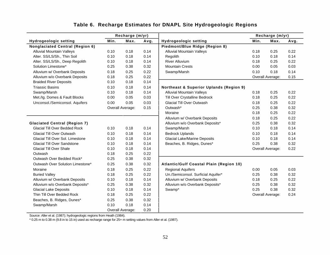
Table 6. Recharge Estimates for DNAPL Site Hydrogeologic Regions
Recharge (m/yr) Recharge (m/yr)Hydrogeologic setting Min. Max. Avg. Hydrogeologic setting Min. Max. Avg.Nonglaciated Central (Region 6) Piedmont/Blue Ridge (Region 8)
Alluvial Mountain Valleys 0.10 0.18 0.14 Alluvial Mountain Valleys 0.18 0.25 0.22 Alter. SS/LS/Sh., Thin Soil 0.10 0.18 0.14 Regolith 0.10 0.18 0.14 Alter. SS/LS/Sh., Deep Regolith 0.10 0.18 0.14 River Alluvium 0.18 0.25 0.22 Solution Limestone* 0.25 0.38 0.32 Mountain Crests 0.00 0.05 0.03 Alluvium w/ Overbank Deposits 0.18 0.25 0.22 Swamp/Marsh 0.10 0.18 0.14 Alluvium w/o Overbank Deposits 0.18 0.25 0.22 Overall Average: 0.15 Braided River Deposits 0.10 0.18 0.14 Triassic Basins 0.10 0.18 0.14 Northeast & Superior Uplands (Region 9)Swamp/Marsh 0.10 0.18 0.14 Alluvial Mountain Valleys 0.18 0.25 0.22 Met./Ig. Domes & Fault Blocks 0.00 0.05 0.03 Till Over Crystalline Bedrock 0.18 0.25 0.22 Unconsol./Semiconsol. Aquifers 0.00 0.05 0.03 Glacial Till Over Outwash 0.18 0.25 0.22
Overall Average: 0.15 Outwash* 0.25 0.38 0.32 Moraine 0.18 0.25 0.22 Alluvium w/ Overbank Deposits 0.18 0.25 0.22
Glaciated Central (Region 7) Alluvium w/o Overbank Deposits* 0.25 0.38 0.32 Glacial Till Over Bedded Rock 0.10 0.18 0.14 Swamp/Marsh 0.10 0.18 0.14 Glacial Till Over Outwash 0.10 0.18 0.14 Bedrock Uplands 0.10 0.18 0.14 Glacial Till Over Sol. Limestone 0.10 0.18 0.14 Glacial Lake/Marine Deposits 0.10 0.18 0.14 Glacial Till Over Sandstone 0.10 0.18 0.14 Beaches, B. Ridges, Dunes* 0.25 0.38 0.32 Glacial Till Over Shale 0.10 0.18 0.14 Overall Average: 0.22 Outwash 0.18 0.25 0.22 Outwash Over Bedded Rock* 0.25 0.38 0.32 Outwash Over Solution Limestone* 0.25 0.38 0.32 Atlantic/Gulf Coastal Plain (Region 10)Moraine 0.18 0.25 0.22 Regional Aquifers 0.00 0.05 0.03 Buried Valley 0.18 0.25 0.22 Un./Semiconsol. Surficial Aquifer* 0.25 0.38 0.32 Alluvium w/ Overbank Deposits 0.10 0.18 0.14 Alluvium w/ Overbank Deposits 0.18 0.25 0.22 Alluvium w/o Overbank Deposits* 0.25 0.38 0.32 Alluvium w/o Overbank Deposits* 0.25 0.38 0.32 Glacial Lake Deposits 0.10 0.18 0.14 Swamp* 0.25 0.38 0.32 Thin Till Over Bedded Rock 0.18 0.25 0.22 Overall Average: 0.24 Beaches, B. Ridges, Dunes* 0.25 0.38 0.32 Swamp/Marsh 0.10 0.18 0.14
Overall Average: 0.20 Source: Aller et al. (1987); hydrogeologic regions from Heath (1984).* 0.25 m to 0.38 m (9.8 in to 15 in) used as recharge range for 25+ m setting values from Aller et al. (1987).
52

Table 7. SSL Dilution Factor Model Results: DNAPL and HGDB Sites
Source area (acres)
0 . 5 1 0 3 0 1 0 0 6 0 0
DNAPL Sites (92)Geomean 34 15 10 6 4Average 321 138 80 44 1910th percentile 3 2 1 1 125th percentile 8 4 3 2 1
Median 30 13 8 5 375th percentile 140 60 35 20 990th percentile 336 144 84 46 20
HGDB sites (208)Geomean 16 10 7 5 3Average 958 829 561 371 159
10th percentile 2 1 1 1 125th percentile 3 2 1 1 1Median 10 6 5 3 275th percentile 56 30 19 12 590th percentile 240 134 90 51 21
All 300 sites
Geomean 20 11 8 6 3Average 763 617 414 271 11610th percentile 2 1 1 1 125th percentile 4 2 2 1 1Median 15 8 5 4 275th percentile 70 35 23 13 690th percentile 292 144 88 49 21
DNAPL = DNAPL Site Survey (EPA/OERR).HGDB = Hydrogeologic database (API).
To adjust the 30-acre DAF for a 0.5-acre source, EPA considered the geomean 0.5-acre dilutionfactors for the DNAPL sites (34), HGDB sites (16), and all 300 sites (20). A default DAF of 20 wasselected as a conservative value for a 0.5-acre source size.
This value also reflects the ratio between 0.5-acre and 30-acre geomean and median dilution factorscalculated for the HGDB sites (2.2 and 2.0, respectively). The HGDB data reflect the influence ofsource size on actual dilution factors more accurately than the DNAPL site data because the HGDBincludes site-specific estimates of aquifer thickness. As shown in the following section, aquiferthickness has a strong influence on the effect of source size on the dilution factor since it provides anupper limit on mixing zone depth. Increasing source area increases infiltration, which lowers thedilution factor, but also increases mixing zone depth, which increases the dilution factor. For aninfinitely thick aquifer, these effects tend to cancel each other, resulting in similar dilution factorsfor 0.5 and 30 acres. Thin aquifers limit mixing depth for larger sources; thus the added infiltrationpredominates and lowers the dilution factors for the larger source. Since the DNAPL dilution factor
53
analyses use a fixed aquifer depth, they tend to overestimate the reduction in dilution factors thatresult from a smaller source.
2.5.7 Sensitivity Analysis. A sensitivity analysis was conducted to examine the effects ofsite-specific parameters on migration to ground water SSLs. Both the partition equation and thedilution factor model were considered in this analysis. Because an adequate database of nationaldistributions of these parameters was not available, a nominal range method was used to conduct theanalysis. In this analysis, independent parameters were selected and each was taken to maximum andminimum values while keeping all other parameters at their nominal, or default, values.
Overall, SSLs are most sensitive to changes in the dilution factor. As shown in Table 7, the 10th to90th percentile dilution factors vary from 2 to 292 for the 300 DNAPL and HGDB sites. Much ofthis variability can be attributed to the wide range of aquifer hydraulic conductivity across the Nation.In contrast, the most sensitive parameter in the partition equation (f oc) only affects the SSL by afactor of 1.5.
Partition Equation. The partition equation requires the following site-specific inputs: fractionorganic carbon, average annual soil moisture content, and soil bulk density. Although volumetric soilmoisture content is somewhat dependent on bulk density (in terms of the porosity available to befilled with water), calculations were conducted to ensure that the parameter ranges selected do notresult in impossible combinations of these parameters. Because the effects of the soil parameters onthe SSLs are highly dependent on chemical properties, the analysis was conducted on four organicchemicals spanning the range of these properties: chloroform, trichloroethylene, naphthalene, andbenzo(a)pyrene.
The range used for soil moisture conditions was 0.02 to 0.43 L water/L soil. The lower end of thisrange represents a likely residual moisture content value for sand, as might be found in the drierregions of the United States. The higher value (0.43) represents full saturation conditions for a loamsoil. The range of bulk density (1.25 to 1.75) was obtained from the Patriot soils database, whichcontains bulk density measurements for over 20,000 soil series across the United States.
Establishing a range for subsurface organic carbon content (foc) was more difficult. In spite of anextensive literature review and contacts with soil scientists, very little information was found on thedistribution of this parameter with depth in U.S. soils. The range used was 0.001 to 0.003 g carbon / gsoil. The lower limit represents the critical organic carbon content below which the partitionequation is no longer applicable. The upper limit was obtained from EPA's Environmental ResearchLaboratory in Ada, Oklahoma, as an expert opinion. Generally, soil organic carbon content falls offrapidly with depth. Since the typical value used as an SSL default for surface soils is 0.006, and 0.002is used for subsurface soils, this limited range is consistent with the other default assumptions used inthe Soil Screening Guidance.
The results of the partition equation sensitivity analysis are shown in Table 8.
For volatile chemicals, the model is somewhat sensitive to water content, with up to 54 and 19percent change in SSLs for chloroform and trichloroethylene, respectively. The model is lesssensitive to bulk density, with a high percent change of 18 for chloroform and 14 fortrichloroethylene. Organic carbon content has the greatest effect on SSLs for all chemicals exceptchloroform. As expected, the effect of foc increases with increasing Koc. The greatest effect was seenfor benzo(a)pyrene whose SSL showed a 50 percent increase at an foc of 0.03. An foc of 0.005 willincrease the benzo(a)pyrene SSL by 150 percent.
54

Table 8. Sensitivity Analysis for SSL Partition Equation
Chloroform Trichloroethylene Naphthalene Benzo(a)pyrene
Parameter assignmentsSSL
(mg/kg)Percentchange
SSL(mg/kg)
Percentchange
SSL(mg/kg)
Percentchange
SSL(mg/kg)
Percentchange
All default parameter values 0.59 — 0.057 — 84 — 8 —
Less conservative parameter valueOrganic carbonBulk densitySoil moisture
0.670.690.74
141826
0.0740.0650.062
29149
1248586
4812
1288
5000
More conservative parameter valueOrganic carbonBulk densitySoil moisture
0.510.510.27
-14-13-54
0.0400.0510.046
-29-10-19
448380
-48-1-4
488
-5000
Conservatism
Input parameters Less Nominal More
Fraction org. carbon(g/g)
0.003 0.002 0.001
Bulk density (kg/L) 1.25a 1.50 1.75b
Average soil moisture(L/L)
0.43 0.30 0.02
a n = 0.53; qa = 0.23.b n = 0.34; qa = 0.04.
Chemical-specific parameters Chloroform Trichloroethylene Naphthalene Benzo(a)pyrene
Koc 3.98E+01 1.66E+02 2.00E+03 1.02E+06
HN 1.50E-01 4.22E-01 1.98E-02 4.63E-05Cw 2.0c 0.1c 20d 0.004c
c MCL H 20 DAF.d HBL (HQ=1) H 20 DAF.
55
Dilution Factor. Site-specific parameters for the dilution factor model include aquifer hydraulicconductivity (K), hydraulic gradient (i), infiltration rate (I), aquifer thickness (d), and source lengthparallel to ground water flow (L). Because they are somewhat dependent, hydraulic conductivity andhydraulic gradient were treated together as Darcy velocity (K H i). The parameter ranges used for thedilution factor analysis represent the 10th and 90th percentile values taken from the HGDB andDNAPL site databases, with the geometric mean serving as the nominal value, as shown in Table 9.
Source length was varied by assuming square sources of 0.5 to 30 acres in size. Bounding estimateswere conducted for each of these source sizes.The results in Table 9 show that Darcy velocity has the greatest effect on the dilution factor, with arange of dilution factors from 1.2 to 85 for a 30-acre source and 2.1 to 263 for a 0.5-acre source.Infiltration rate has the next highest effect, followed by source size and aquifer thickness. Note thataquifer thickness has a profound effect on the influence of source size on the dilution factor. Thickaquifers show no source size effect because the increase in infiltration flux from a larger source isbalanced by the increase in mixing zone depth, which increases dilution in the aquifer. For very thinaquifers, the mixing zone depth is limited by the aquifer thickness and the increased infiltration fluxpredominates, decreasing the dilution factor for larger sources.
2 .6 Mass-Limit Model Development
This section describes the development of models to solve the mass-balance violations inherent inthe infinite source models used to calculate SSLs for the inhalation and migration to ground waterexposure pathways. The models developed are not finite source models per se, but are designed foruse with the current infinite source models to provide a lower, mass-based limit for SSLs for themigration to ground water and inhalation exposure pathways for volatile and leachable contaminants. For each pathway, the mass-limit model calculates a soil concentration that corresponds to therelease of all contaminants present within the source, at a constant health-based concentration, overthe duration of exposure. These mass-based concentration limits are used as a minimumconcentration for each SSL; below this concentration, a receptor point concentration time-averagedover the exposure period cannot exceed the health-based concentration on which it is based.
2.6.1 Mass Balance Issues. Infinite source models are subject to mass balance violationsunder certain conditions. Depending on a compound's volatility and solubility and the size of thesource, modeled volatilization or leaching rates can result in a source being depleted in a shorter timethan the exposure duration (or the flux over a 30- or 70-year duration would release a greater mass ofcontaminants than are present). Several commenters to the December 1994 draft Soil ScreeningGuidance expressed concern that it is unrealistic for total emissions over the duration of exposure toexceed the total mass of contaminants in a source. Using the soil saturation concentration (Csat) anda 5- to 10-meter contaminant depth, one commentor calculated that mass balance would be violatedby the SSL volatilization model for 25 percent of the SSL chemicals.
Short of finite source modeling, the limitations of which in soil screening are discussed in the draftTechnical Background Document for Soil Screening Guidance (U.S. EPA, 1994i), there were twooptions identified for addressing mass-balance violations within the soil screening process:
• Shorten the exposure duration to a value that would reflect masslimitations given the volatilization rate calculated using the currentmethod
56

Table 9. Sensitivity Analysis for SSL Dilution Factor Model
Dilution Factor
Source area
Ratio of 0.5-acre/30-acre
Mixing depth (m)
Parameterassignments 30-acre 0.5-acre 30-acre 0.5 acre
All central parameters 5.2 15 2.9 12 5.1
Less conservativeDarcy velocityAquifer thicknessInfiltration rate
851539
26315
118
3.11.03.0
124012
4.85.14.8
More conservativeDarcy velocityAquifer thicknessInfiltration rate
1.22.13.2
2.19.18.7
1.84.32.7
123.012
123.05.5
Conservatism
Input parameters Less Nominal More
Darcy velocity (DV, m/yr) 442 22 0.8
Aquifer thickness (da, m) 46 12 3
Infiltration rate (m/yr) 0.02 0.18 0.35
Parameter sources
Percentile DVa (m/yr) dab (m)
10th 0.8 3.0
25th 4 5.5
50th 22 11
75th 121 23
90th 442 46
Average: 800 28
Geomean: 22 12a 300 DNAPL & HGDB sites.b 208 HGDB sites.
57

• Change the volatilization rate to a value corresponding to the uniformrelease of the total mass of contaminants over the period of exposure.
The latter approach was taken in the draft Risk-Based Corrective Action (RBCA) screeningmethodology developed by the American Society for Testing and Materials (ASTM) (ASTM, 1994).As stated on page B6 of the RBCA guidance (B.6.6.6):
In the event that the time-averaged flux exceeds that which would occur if allchemicals initially present in the surficial soil zone volatilized during the exposureperiod, then the volatilization factor is determined from a mass balance assuming thatall chemical initially present in the surficial soil zone volatilizes during the exposureperiod.
This was selected over the exposure duration option because it is reasonably conservative forscreening purposes (obviously, more contaminant cannot possibly volatilize from the soil) and itavoided the uncertainties associated with applying the current models to estimate source depletionrates.
In summary, the mass-limit approach offers the following advantages:
• It corrects the possible mass-balance violation in the infinite-sourceSSLs.
• It does not require development of a finite source model to calculateSSLs.
• It is appropriate for screening, being based on the conservativeassumption that all of the contaminant present leaches or volatilizesover the period of exposure.
• It is easy to develop and implement, requiring only very simplealgebraic equations and input parameters that are, with the exceptionof source depth, already used to calculate SSLs.
The derivation of these models is described below. It should be noted that the American IndustrialHealth Council (AIHC) independently developed identical models to solve the mass-balance violationas part of their public comments on the Soil Screening Guidance.
2.6.2 Migration to Ground Water Mass-Limit Model. For the migration to groundwater pathway, the mass of contaminant leached from a contaminant source over a fixed exposureduration (ED) period can be calculated as
Ml = Cw H I H As H ED (47)
where
Ml = mass of contaminant leached (g)Cw = leachate contaminant concentration (mg/L or g/m3)I = infiltration rate (m/yr)As = source area (m2)ED = exposure duration (yr).
58

The total mass of contaminants present in a source can be expressed as
MT = Ct Hρb H As H ds (48)
where
MT = total mass of contaminant present (g)Ct = total soil contaminant concentration (mg/kg or g/Mg, dry basis)ρb = dry soil bulk density (kg/L or Mg/m3)As = source area (m2)ds = source depth (m).
To avoid a mass balance violation, the mass of contaminant leached cannot exceed the total mass ofcontaminants present (i.e., Ml cannot exceed MT). Therefore, the maximum possible contaminantmass that can be leached from a source (assuming no volatilization or degradation) is MT and theupper limit for Ml is
Ml = MT
or
Cw × I × As × ED = Ct × ρb × As × ds
Rearranging to solve for the total soil concentration (Ct) corresponding to this situation (i.e.,maximum possible leaching)
Mass-Limit Model for Migration to Ground Water Pathway
Ct = (Cw × I × ED)/(ρb × ds) (49)
Parameter/Definition (units) Default
Ct/screening level in soil (mg/kg) --
Cw/target soil leachate concentration (mg/L) (nonzero MCLG, MCL, or HBL) × 20 DAF
I/infiltration rate (m/yr) site-specificED/exposure duration (yr) 70ρb/dry soil bulk density (kg/L) 1.5
ds/average source depth (m) site-specific
59

This soil concentration (Ct) represents a lower limit for soil screening levels calculated for themigration to ground water pathway. It represents the soil concentration corresponding to completerelease of soil contaminants over the ED time period at a constant soil leachate concentration (C w).Below this Ct, the soil leachate concentration averaged over the ED time period cannot exceed Cw.
2.6.3 Inhalation Mass-Limit Model. The volatilization factor (VF) is basically the ratioof the total soil contaminant concentration to the air contaminant concentration. VF can becalculated as
VF = (Q/C) H (CTo/Jsave) H 10-10 m2kg/cm2mg (50)
where
VF = volatilization factor (m3/kg)Q/C = inverse concentration factor for air dispersion (g/m2-s per kg/m3)CTo = total soil contaminant concentration at t=0 (mg/kg or g/Mg, dry basis)Jsave = average rate of contaminant flux from the soil to the air (g/cm2-s).
The total amount of contaminant contained within a finite source can be written as
Mt = CTo H ρb H As H ds (51)
where
Mt = total mass of contaminant within the source (g)CTo = total soil contaminant concentration at t=0 (mg/kg or g/Mg, dry basis)ρb = soil dry bulk density (kg/L = Mg/m3)As = area of source (m2)ds = depth of source (m).
If all of the contaminant contained within a finite source is volatilized over a given averaging timeperiod, the average volatilization flux can be calculated as
Jsave = Mt/[(As H 104 cm2/m2) H (T H 3.15E7 s/yr)] (52)
where
T = exposure period (yr).
Substituting Equation 51 for Mt in Equation 52 yields
Jsave = (CTo H ρb H ds) / (104 cm2/m2 H T H 3.15E7 s/yr) (53)
Rearranging Equation 53 yields
60

CTo/Jsave = (104 cm2/m2 H T H 3.15E7 s/yr)/(ρb H ds) (54)
Substituting Equation 54 into Equation 50 yields
Mass-Limit Model for Inhalation of Volatiles
VF = (Q/C) H [(T H 3.15E7 s/yr)/(ρb H ds H 106 g/Mg)] (55)
Parameter/Definition (units) Default
VF/volatilization factor (m3/kg) --Q/C/inverse of mean conc. at center of source (g/m2-s per kg/m3) Table 3T/exposure interval (yr) 30ρb/dry soil bulk density (kg/L) 1.5
ds/average source depth (m) site-specific
If the VF calculated using an infinite source volatilization model for a given contaminant is less thanthe VF calculated using Equation 55, then the assumption of an infinite source may be tooconservative for that specific contaminant at that source. Consequently, VF, as calculated inEquation 55, could be considered a minimum value for VF.
2 .7 Plant Uptake
Commentors have raised concerns that the ingestion of contaminated produce from homegrowngardens may be a significant exposure pathway. EPA evaluated empirical data on plant uptake,particularly the data presented in the Technical Support Document for Land Application of SewageSludge, often referred to as the "Sludge Rule" (U.S. EPA, 1992d).
EPA found that empirical plant uptake-response slopes were available for selected metals but thatavailable data were insufficient to estimate plant uptake of organics. In an effort to obtain additionalempirical data, EPA has jointly funded research with the State of California on plant uptake oforganic contaminants. These studies support ongoing revisions to the indirect, multimedia exposuremodel CalTOX.
The Sludge Rule identified six metals of concern with empirical plant uptake data: arsenic, cadmium,mercury, nickel, selenium, and zinc. Plant uptake-response slopes were given for seven plantcategories such as grains and cereals, leafy vegetables, root vegetables, and garden fruits. EPAevaluated the study conditions (e.g., soil pH, application matrix) and methods (e.g., geometric mean,default values) used to calculate the plant uptake-response slopes for each plant category anddetermined that the geometric mean slopes were generally appropriate for calculating SSLs for thesoil-plant-human exposure pathway.
However, the geometric mean of empirical uptake-response slopes from the Sludge Rule must beinterpreted with caution for several reasons. First, the dynamics of sludge-bound metals may differfrom the dynamics of metals at contaminated sites. For example, the empirical data were derived
61

from a variety of studies at different soil conditions using different forms of the metal (i.e., salt vs.nonsalt). In studies where the application matrix was sludge, the adsorption power of sludge in thepresence of calcium ions may have reduced the amount of metal that is bioavailable to plants and,therefore, plant uptake may be greater in non-sludge-amended soils.
In addition to these confounding conditions, default values of 0.001 were assigned for plant uptake instudies where the measured value was below 0.001. A default value was needed to calculate thegeometric mean uptake-response slope values. Moreover, considerable study-to-study variability isshown in the plant uptake-response slope values (up to 3 orders of magnitude for certain plant/metalcombinations). This variability could result from varying soil characteristics or experimentalconditions, but models have not been developed to relate changes in plant uptake to such conditions.Thus, the geometric mean values represent "typical" values from the experiments; actual values atspecific sites could show marked variation depending on soil composition, chemistry, and/or planttype.
OERR has used the information in the Sludge Rule to identify six metals (arsenic, cadmium, mercury,nickel, selenium, and zinc) of potential concern through the soil-plant-human exposure pathway forconsideration on a site-specific basis. The fact that these metals have been identified should not bemisinterpreted to mean that other contaminants are not of potential concern for this pathway.Other EPA offices are looking at empirical data and models for estimating plant uptake of organiccontaminants from soils and OERR will incorporate plant uptake of organics once these efforts arereviewed and finalized.
Methods for evaluating the soil-plant-human pathway are presented in Appendix G. Genericscreening levels are calculated based on the uptake factors (i.e., bioconcentration factors [Br])presented in the Sludge Rule. Generic plant SSLs are compared with generic SSLs based on directingestion as well as levels of inorganics in soil that have been reported to cause phytotoxicity (Willand Suter, 1994). Although site-specific factors such as soil type, pH, plant type, and chemical formwill determine the significance of this pathway, the results of our analysis suggest that the soil-plant-human pathway may be of particular concern for sites with soils contaminated with arsenic orcadmium. Likewise, the potential for phytotoxicity will be greatly influenced by site-specific factors;however, the data presented by Will and Suter (1994) suggest that, with the exception of arsenic, thelevels of inorganics that are considered toxic to plants are well below the levels that may impacthuman health via the soil-plant-human pathway.
2 .8 Intrusion of Volatiles into Basements: Johnson and Ettinger Model
Concern about the potential impact of contaminated soil on indoor air quality prompted EPA toconsider the Johnson and Ettinger (1991) model, a heuristic model for estimating the intrusion rateof contaminant vapors from soil into buildings. The model is a closed-form analytical solution forboth convective and diffusive transport of vapor-phase contaminants into enclosed structures locatedabove the contaminated soil. The model may be solved for both steady-state (i.e., infinite source) orquasi-steady-state (i.e., finite source) conditions. The model incorporates a number of keyassumptions, including no leaching of contaminant to ground water, no sinks in the building, and well-mixed air volume within the building.
To evaluate the effects of using the Johnson and Ettinger model on SSLs for volatile organiccontaminants, EPA contracted Environmental Quality Management, Inc. (EQ), to construct a caseexample to estimate a high-end exposure point concentration for residential land use (Appendix H;EQ and Pechan, 1994). The case example models a contaminant source relatively close or directlybeneath a building where the soil beneath the building is very permeable and the building is
62

underpressurized, tending to pull contaminants into the basement. Where possible and appropriate,values of model variables were taken directly from Johnson and Ettinger (1991). Using both steady-state and quasi-steady-state formulations, building air concentrations of each of 42 volatile SSLchemicals were calculated. The inverses of these concentrations were substituted into the inhalationSSL equations (Equations 4 or 5) as an indoor volatilization factor (VF indoor) to calculate carcinogenicor noncarcinogenic SSLs based on migration of contaminants into basements (i.e., "indoorinhalation" SSLs).
Results showed a difference of up to 2 orders of magnitude between the steady-state and quasi-steady-state results for the indoor inhalation SSLs. Infinite source indoor inhalation SSLs were less than thecorresponding "outdoor" inhalation SSLs by as much as 3 orders of magnitude for highly volatileconstituents. For low-volatility constituents, the difference was considerably less, with no differencein the indoor and outdoor SSLs in some cases. The EQ study also indicated that the most importantinput parameters affecting long-term building concentration (and thus the SSL) are buildingventilation rate, distance from the source (i.e., source-building separation), soil permeability to vaporflow, and source depth. For lower-permeability soils, the number and size of cracks in the basementwalls may be more significant, although this was not a significant variable for the permeable soilsconsidered in the study.
EPA decided against using the Johnson and Ettinger model to calculate generic SSLs due to thesensitivity of the model to parameters that do not lend themselves to standardization on a nationalbasis (e.g., source depth, the number and size of cracks in basement walls). In addition, the onlyformal validation study identified by EPA compares model results with measured radonconcentrations from a highly permeable soil. Although these results compare favorably, it is notclear how applicable they are to less permeable soils and compounds not already present in soil as agas (as radon is).
The model can be applied on a site-specific basis in conjunction with the results of a soil gas survey.Where land use is currently residential, a soil gas survey can be used to measure the vapor phaseconcentrations at the foundation of buildings, thereby eliminating the need to model partitioning ofcontaminants, migration from the source to the basement, and soil permeability.
For future use scenarios, although some site-specific data are available, the difficulties are similar tothose encountered with generic application of the model. Predictions must be made regarding thedistance from the source to the basement and the permeability of the soil, basement floor, and walls.EQ's report models the potential impact of placing a structure directly above the source. Dependingon the permeability of the surrounding soils, the results suggest that the level of residualcontamination would have to be extremely low to allow for such a scenario. Distance from the sourcecan have a dramatic impact on the results and should be considered in more detailed investigationsinvolving future residential use scenarios.
63

Part 3: MODELS FOR DETAILED ASSESSMENT
The Soil Screening Guidance addresses the inhalation and migration to ground water exposurepathways with simple equations that require a small number of easily obtained soil parameters,meteorologic conditions, and hydrogeologic parameters. These equations incorporate a number ofconservative simplifying assumptions—an infinite source, no fractionation between pathways, nobiological or chemical degradation, no adsorption—conditions that can be addressed with morecomplicated models. Applying such models will more accurately define the risk of exposure via theinhalation or the migration to ground water pathway and, depending on site conditions, can lead tohigher SSLs that are still protective. However, input data requirements and modeling costs make thisoption more expensive to implement than the SSL equations.
This part of the Technical Background Document presents information on the selection and use ofmore complex fate and transport models for calculating SSLs. Generally, the decision to use thesemodels will involve balancing costs: if the models and assumptions used to develop simple site-specific SSLs are overly conservative with respect to site conditions (e.g., a thick unsaturated zone),the additional cost and time required to apply these models may be offset by the potential costsavings associated with higher, but still protective, SSLs.
Sections 3.1 and 3.2 include information on equations and models that can accommodate finitecontaminant sources and fractionate contaminants between pathways (e.g., VLEACH and EMSOFT)and predict the subsequent impact on either ambient air or ground water. However, when using afinite source model, the site manager should recognize the uncertainties inherent in site-specificestimates of subsurface contaminant distributions and use conservative estimates of source size andconcentrations to allow for such uncertainties. In addition, model predictions should be validatedagainst actual site conditions to the extent possible.
3 .1 Inhalation of Volatiles: Detailed Models
Developing SSLs for the inhalation of volatiles involves calculating a site-specific volatilizationfactor (VF) and dispersion factor (Q/C). This section provides a brief description of finite sourcevolatilization models with potential applicability to SSL development and information on site-specific application of the AREA-ST dispersion model for estimating the Q/C values needed tocalculate both VF and PEF. It should not be viewed as an official endorsement of these models (othervolatilization models may be available with applicability to SSL development).
3.1.1 Finite Source Volatilization Models. To identify suitable models for addressing afinite contaminant source, EPA contracted Environmental Quality Management, Inc. (EQ), toconduct a preliminary evaluation of a number of soil volatilization models, including volatilizationmodels developed by Hwang and Falco (1986), as modified by EQ (1992), and by Jury et al. (1983,1984, and 1990) and VLEACH, a multipathway model developed primarily to assess exposurethrough the ground water pathway. Study results (EQ and Pechan, 1994) show reasonable agreement(within a factor of 2) between emission predictions using the modified Hwang and Falco or Jurymodels, but consistently lower predictions from VLEACH. However, Shan and Stephens (1995)discovered an error in the VLEACH calculation of the apparent diffusivity, which has beensubsequently corrected. The corrected VLEACH model, version 2.2, appears to provide emissionestimates similar to the Jury and the modified Hwang and Falco models. The revised VLEACH (v.2.2)
64

program is available from the Center for Subsurface Modeling Support (CSMOS) at EPA'sEnvironmental Research Laboratory in Ada, Oklahoma (WWW.EPA.GOV/ADA/ CSMOS.HTML),and is discussed further in Section 3.2.
For certain contaminant conditions, Jury et al. (1990) present a simplified equation (Jury's EquationB1) for estimating the flux of a contaminant from a finite source of contaminated soil. Thefollowing assumptions were used to derive this simplified flux equation:
• Uniform soil properties (e.g., homogeneous average soil water content, bulk density,porosity, and fraction organic carbon)
• Instantaneous linear equilibrium adsorption
• Linear equilibrium liquid-vapor partitioning (Henry's law)
• Uniform initial contaminant incorporation at t=0
• Chemicals in a dissolved form only (i.e., soil contaminant concentrations are belowCsat)
• No boundary layer thickness at ground level (no stagnant air layer)
• No water evaporation or leaching
• No chemical reactions, biodegradation, or photolysis
• ds >> (4DAt)1/2 (ramifications of this are discussed below).
Under these assumptions, the Jury et al. (1990) simplified finite source model is
Js = Co(DA/πt)1/2[1-exp(-ds2/4DAt)] (56)
whereJs = contaminant flux at ground surface (g/cm2-s)
Co = uniform contaminant concentration at t=0 (g/cm3)DA = apparent diffusivity (cm2/s)
π = 3.14t = time (s)
ds = depth of uniform soil contamination at t=0 (cm),
and
DA = [(θa10/3 Di HN + θw10/3 Dw)/n2]/(ρb Kd + θw + θa HN) (57)
whereθa = air-filled soil porosity (Lair/Lsoil) = n - θwn = total soil porosity (Lpore/Lsoil) = 1 - (ρb/ρs)
θw = water-filled soil porosity (Lwater/Lsoil) = wρb/ρw
ρb = soil dry bulk density (g/cm3)ρs = soil particle density (g/cm3)w = average soil moisture content (g/g)
65

ρw = water density (g/cm3)Di = diffusivity in air (cm2/s)HN = dimensionless Henry's law constant = 41 H HLC
HLC = Henry's law constant (atm-m3/mol)Dw = diffusivity in water (cm2/s)Kd = soil-water partition coefficient (cm3/g) = Koc foc
Koc = soil organic carbon partition coefficient (cm3/g)foc = organic carbon content of soil (g/g).
To estimate the average contaminant flux over 30 years, the time-dependent contaminant fluxmust be solved for various times and the results averaged. A simple computer program orspreadsheet can be used to calculate the instantaneous flux of contaminants at set intervals andnumerically integrate the results to estimate the average contaminant flux. However, the time-stepinterval must be small enough (e.g., 1-day intervals) to ensure that the cumulative loss throughvolatilization is less than the total initial mass. Inadequate time steps can lead to mass-balanceviolations.
To address this problem, EPA/ORD’s National Center for Environmental Assessment has developeda computer modeling program, EMSOFT. The computer program provides an average emission fluxover time by using an analytical solution to the integral, thereby eliminating the problem ofestablishing adequate time steps for numerical integration. In addition, the EMSOFT model canaccount for water convection (i.e., leaching), and the impact of a soil-air boundary layer on the fluxof contaminants with low Henry’s law constants. EMSOFT will be available through EPA’s NationalCenter for Environmental Assessment (NCEA) in Washington, DC.
Once the average contaminant flux is calculated, VF is calculated as:
VF = (Q/C) H (Co/ρb) H (1/Jsave) H 10-4 m2/cm2 (58)
where
VF = volatilization factor (m3/kg)Q/C = inverse concentration factor for air dispersion (g/m2-s per kg/m3)
Co = uniform contaminant concentration at t=0 (g/cm3)ρb = soil dry bulk density (g/cm3)
Jsave = average rate of contaminant flux (g/cm2-s).
3.1.2 Air Dispersion Models. The inverse concentration factor for air dispersion, Q/C, isused in the determination of both VF and PEF. For a detailed site-specific assessment of theinhalation pathway, a site-specific Q/C can be determined using the Industrial Source Complex Modelplatform in the short-term mode (ISCST3). Only a very brief overview of the application,assumptions, and input requirements for the model as used to determine Q/C is provided in thissection. This model is the final regulatory version of the ISCST3 model.
The ISCST3 model FORTRAN code, executable versions, sample input and output files, description,and documentation can be downloaded from the “Other Models” section of the Office of Air QualityPlanning and Standards (OAQPS) Support Center for Regulatory Air Models bulletin board system(SCRAM BBS). To access information, call:
66

OAQPS SCRAM BBS(919) 541-5742 (24 hours/day, 7 days/week except Monday AM)1,200–9,600, 14,400 baudLine Settings: 8 bits, no parity, 1 stop bitTerminal Emulation: VT100 or ANSISystem Operator: (919) 541-5384 (normal business hours EST).
The user registers in the first call and then has full access to the BBS.
The ISCST3 model will output an air concentration (in µg/m3) when the concentration model optionis selected (e.g., CO MODELOPT DFAULT CONC rural/urban). The surface area of thecontaminated soil source must be determined. For the ISCST3 model, the source location of an areasource is defined by the coordinates of the southwest corner of the square (e.g., SO LOCATIONsourcename AREA -1/2length -1/2width height=0). For the source parameter input line, thecontaminant's area emission rate (in units of g/m2-s) must be entered. The area emission rate is thesite-specific average emission flux rate, as calculated in Equation 56, converted to units of g/m2-s(i.e., Aremis = Jsave H 104 cm2/m2). Alternatively, an area emission rate of 1 g/m2-s can be assumed.A grid or circular series of receptor sites should be used in and around the area source to identify thepoint of maximum contaminant air concentration. Hourly meteorologic data (*.MET files) for thenearest city (i.e., airport) of similar terrain and the preprocessor PCRAMMET also can bedownloaded from the SCRAM BBS.
The ISCST3 model output concentration is then used to calculate Q/C as
Q/C = (Jsave H 104 cm2/m2)/(Cair H 10-9 kg/µg) (59)
where
Q/C = inverse concentration factor for air dispersion (g/m2-s per kg/m3)Jsave = average rate of contaminant flux (g/cm2-s)Cair = ISC output maximum contaminant air concentration (µg/m3).
Note: If an area emission rate of 1 g/m2-s is assumed, then (Jsave H 104 cm2/m2) = 1, and Equation59 simplifies to simply the inverse of the maximum contaminant air concentration (inkg/m3).
3 .2 Migration to Ground Water Pathway
For the migration to ground water pathway, the SSL equations assume an infinite source,contamination extending to the water table, and no attenuation due to degradation or adsorption inthe unsaturated zone. At sites with small sources, deep water tables, confining layers in theunsaturated zone that can block contaminant transport, or contaminants that degrade throughbiological or chemical mechanisms, more complex models that can address such site conditions canbe used to calculate higher SSLs that still will be protective of ground water quality. This sectionprovides information on the use of such models in the soil screening process to calculate a dilution-attenuation factor (Section 3.2.1) and to estimate contaminant release in leachate and transportthrough the unsaturated zone (Section 3.2.2).
67

3.2.1 Saturated Zone Models. EPA has developed guidance for the selection andapplication of saturated zone transport and fate models and for interpretation of model applications.The user is referred to Ground Water Modeling Compendium, Second Edition 1994 (U.S. EPA,1994b) and Framework for Assessing Ground Water Modeling Applications (U.S. EPA, 1994a) forfurther information.
More complex saturated zone models can be used to calculate a dilution-attenuation factor (DAF)that, unlike the SSL dilution model, can consider attenuation in the aquifer. Some can handle a finitesource through a transient mode that requires a time-stepped concentration from a finite-sourceunsaturated zone model (see Section 3.2.2). In general, to calculate a DAF using such models, thecontaminant concentration at the water table under the source (Cw) is set to unity (e.g., 1 mg/L).The DAF is the reciprocal of the predicted concentration at the receptor point (CRP) as follows:
DAF = Cw /CRP = 1/CRP (60)
3.2.2 Unsaturated Zone Models. In an effort to provide useful information for modelapplication, EPA's ORD laboratories in Ada, Oklahoma, and Athens, Georgia, conducted anevaluation of nine unsaturated zone fate and transport models (Criscenti et al., 1994; Nofziger et al.,1994). The results of this effort are summarized here. The models reviewed are only a subset of thepotentially appropriate models available to the public and are not meant to be construed as havingreceived EPA approval. Other models also may be applicable to SSL development, depending on site-specific circumstances.
Each of the unsaturated zone models selected for evaluation are capable, to varying degrees, ofsimulating the transport and transformation of chemicals in the subsurface. Even the most unique siteconditions can be simulated by either a single model or a combination of models. However, theintended uses and the required input parameters of these models vary. The models evaluated include:
• RITZ (Regulatory and Investigative Treatment Zone model)
• VIP (Vadose zone Interactive Process model)
• CMLS (Chemical Movement in Layered Soils model)
• HYDRUS
• SUMMERS (named after author)
• MULTIMED (MULTIMEDia exposure assessment model)
• VLEACH (Vadose zone LEACHing model)
• SESOIL (SEasonal SOIL compartment model)
• PRZM-2 (Pesticide Root Zone Model).
RITZ, VIP, CMLS, and HYDRUS were evaluated by Nofziger et al. (1994). SUMMERS,MULTIMED, VLEACH, SESOIL, and PRZM-2 were evaluated by Criscenti et al. (1994). Thesedocuments should be consulted for further information on model application and use.
The applications, assumptions, and input requirements for the nine models evaluated are described inthis section. The model descriptions include model solution method (i.e., analytical, numerical), the
68
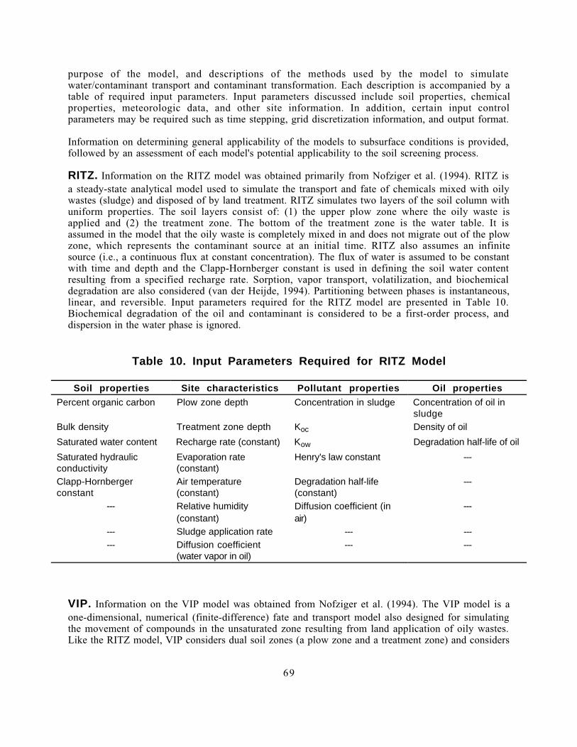
purpose of the model, and descriptions of the methods used by the model to simulatewater/contaminant transport and contaminant transformation. Each description is accompanied by atable of required input parameters. Input parameters discussed include soil properties, chemicalproperties, meteorologic data, and other site information. In addition, certain input controlparameters may be required such as time stepping, grid discretization information, and output format.
Information on determining general applicability of the models to subsurface conditions is provided,followed by an assessment of each model's potential applicability to the soil screening process.
RITZ. Information on the RITZ model was obtained primarily from Nofziger et al. (1994). RITZ isa steady-state analytical model used to simulate the transport and fate of chemicals mixed with oilywastes (sludge) and disposed of by land treatment. RITZ simulates two layers of the soil column withuniform properties. The soil layers consist of: (1) the upper plow zone where the oily waste isapplied and (2) the treatment zone. The bottom of the treatment zone is the water table. It isassumed in the model that the oily waste is completely mixed in and does not migrate out of the plowzone, which represents the contaminant source at an initial time. RITZ also assumes an infinitesource (i.e., a continuous flux at constant concentration). The flux of water is assumed to be constantwith time and depth and the Clapp-Hornberger constant is used in defining the soil water contentresulting from a specified recharge rate. Sorption, vapor transport, volatilization, and biochemicaldegradation are also considered (van der Heijde, 1994). Partitioning between phases is instantaneous,linear, and reversible. Input parameters required for the RITZ model are presented in Table 10.Biochemical degradation of the oil and contaminant is considered to be a first-order process, anddispersion in the water phase is ignored.
Table 10. Input Parameters Required for RITZ Model
Soil properties Site characteristics Pollutant properties Oil properties
Percent organic carbon Plow zone depth Concentration in sludge Concentration of oil insludge
Bulk density Treatment zone depth Koc Density of oil
Saturated water content Recharge rate (constant) Kow Degradation half-life of oil
Saturated hydraulicconductivity
Evaporation rate(constant)
Henry's law constant ---
Clapp-Hornbergerconstant
Air temperature(constant)
Degradation half-life(constant)
---
--- Relative humidity(constant)
Diffusion coefficient (inair)
---
--- Sludge application rate --- ------ Diffusion coefficient
(water vapor in oil)--- ---
VIP. Information on the VIP model was obtained from Nofziger et al. (1994). The VIP model is aone-dimensional, numerical (finite-difference) fate and transport model also designed for simulatingthe movement of compounds in the unsaturated zone resulting from land application of oily wastes.Like the RITZ model, VIP considers dual soil zones (a plow zone and a treatment zone) and considers
69

the source to be infinite. VIP differs from RITZ in that it solves the governing differential equationsnumerically, which allows variability in the flux of water and chemicals over time. Advection andhydrodynamic dispersion are the primary transport mechanisms for the contaminant in water (vander Heijde, 1994). Instead of assuming instantaneous, linear equilibrium between all phases, VIPconsiders the partitioning rates between the air, oil, soil, water, and vapor-phase transport.Contaminant transformation processes include hydrolysis, volatilization, and sorption. Oxygen-limited degradation and diffusion of the contaminant in the air phases are also considered. Sorption isinstantaneous as described for the RITZ model. The input parameters required for the VIP model arepresented in Table 11.
Table 11. Input Parameters Required for VIP Model
Soil properties
Site characteristics
Pollutant properties Oxygen properties
Oilproperties
Porosity Plow zone depth Concentration insludge
Oil-air partitioncoefficienta
Density of oil
Bulk density Treatment zonedepth
Oil-water partitioncoefficienta
Water-air partitioncoefficienta
Degradationrate constantof oil
Saturated hydraulicconductivity
Mean dailyrecharge rate
Air-water partitioncoefficienta
Oxygen half-saturationconstant in air phase a
---
Clapp-Hornbergerconstant
Temperature (eachlayer)
Soil-water partitioncoefficienta
Oxygen half-saturationconstant in oil phase a
---
--- Sludge applicationrate
Degradation constantin oila
Oxygen half-saturationconstant in waterphasea
---
--- Sludge density Degradation constantin watera
Oxygen half-saturationconstant (oildegradation)
---
--- Application periodand frequency inperiod
Dispersion coefficient Stoichiometric ratio ofoxygen to pollutantconsumed
---
--- Weight fractionwater in sludge
Adsorption-desorptionrate constant (water/oil)
Stoichiometric ratio ofoxygen to oilconsumed
---
--- Weight fraction oilin waste
Adsorption-desorptionrate constant(water/soil)
Oxygen transfer ratecoefficient between oiland air phases
---
--- --- Adsorption-desorptionrate constant (water/air)
Oxygen transfer ratecoefficient betweenwater and air phases
---
a Parameters required for plow zone and treatment zone.
CMLS . Information on CMLS was obtained from Nofziger et al. (1994). CMLS is an analyticalmodel developed as a management tool to describe the fate and transport of pesticides in layered soilsand to estimate the amount of chemical at a certain position at a certain time. The model allowsdesignation of up to 20 soil layers with uniform soil and chemical properties defined for each layer.
70

Water in the soil system is "pushed ahead" of new water (recharge) entering the system. The watercontent is reduced to the field capacity after each infiltration event, and water is removed from theroot zone in proportion to the available water stored in that layer (Nofziger et al., 1994). CMLSassumes movement of the chemical in liquid phase only and allows a finite source. Chemicalpartitioning between the soil and the water is assumed to be linear, instantaneous, and reversible.Volatilization is not considered. Dispersion and diffusion of the chemical is ignored and degradation isdefined as a first-order process. The input parameters required for the CMLS model are presented inTable 12.
Table 12. Input Parameters Required for CMLS
Soil properties Site characteristics Chemical properties
Depth of bottom of soil layers Daily infiltration or precipitation Degradation half-life (each soil layer)
Organic carbon content Daily evapotranspiration Amount appliedBulk density --- Depth of applicationSaturated water content --- Date of applicationField capacity --- Koc
Permanent wilting point --- ---
HYDRUS . Information on the HYDRUS model was obtained from Nofziger et al. (1994).HYDRUS is a finite-element model for one-dimensional solute fate and transport simulations. Theboundary conditions for flow, as well as soil and chemical properties, can therefore vary with time. Afinite source also can be modeled. Soil parameters are described by the van Genuchten parameters.The model also considers root uptake and hysteresis in the water movement properties. Solutetransport and transformation incorporates molecular diffusion, hydrodynamic dispersion, linear ornonlinear equilibrium partitioning (sorption), and first-order decay (van der Heijde, 1994).Volatilization is not considered. The input parameters required by HYDRUS are presented inTable 13.
SUMMERS . Information on the SUMMERS model was obtained from Criscenti et al. (1994).SUMMERS is a one-dimensional analytical model that simulates one-dimensional, nondispersivetransport in a single layer of soil from an infinite source. It was developed to determine thecontaminant concentrations in soil that would result in ground water contamination above specifiedlevels for evaluating geothermal energy sites. The model is similar to the SSL equations in that itassumes steady-state water movement and equilibrium partitioning of the contaminant in theunsaturated zone and performs a mass-balance calculation of mixing in an underlying aquifer. For thesaturated zone, the model assumes a constant flux from the surface source and instantaneous,complete mixing in the aquifer. The mixing depth is therefore defined by the thickness of theaquifer. The model does not account for volatilization. The input parameters required for SUMMERSare listed in Table 14.
71
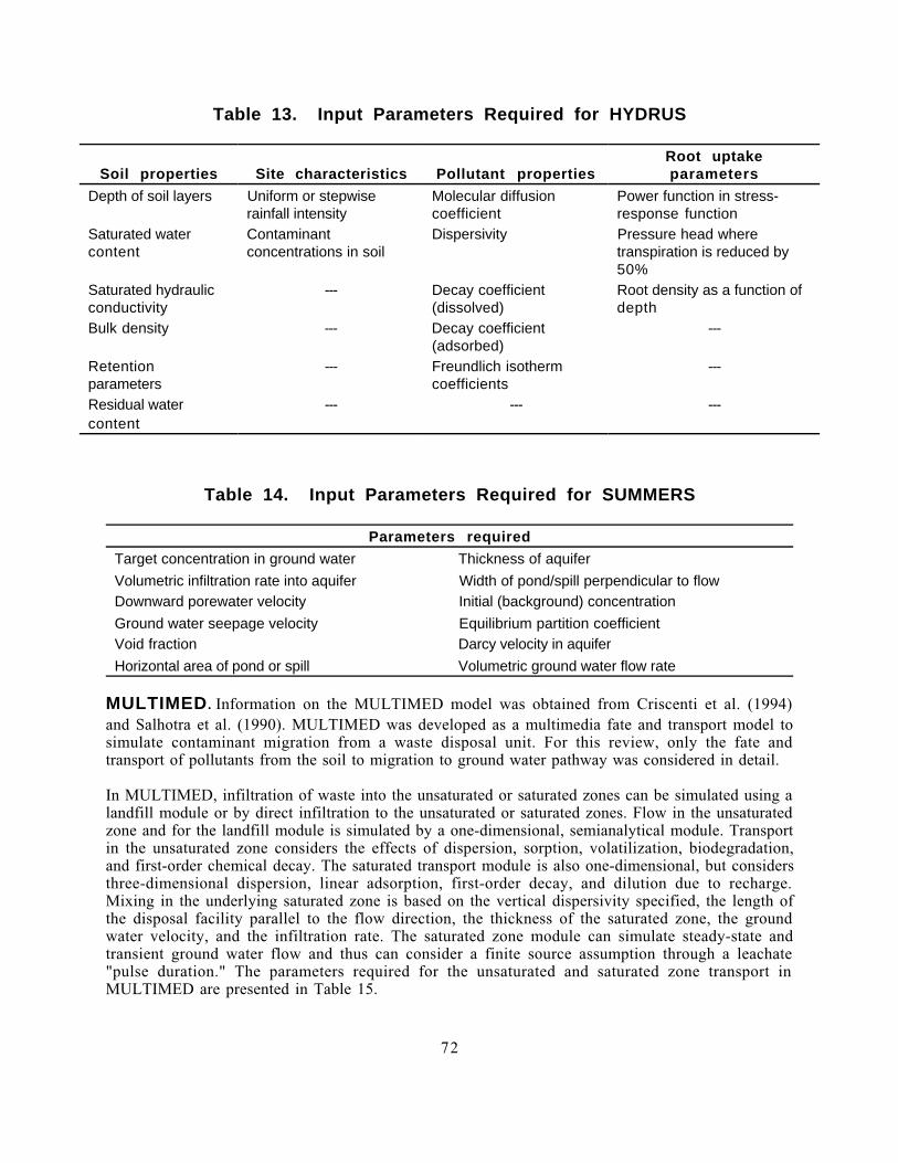
Table 13. Input Parameters Required for HYDRUS
Soil properties Site characteristics Pollutant propertiesRoot uptakeparameters
Depth of soil layers Uniform or stepwiserainfall intensity
Molecular diffusioncoefficient
Power function in stress-response function
Saturated watercontent
Contaminantconcentrations in soil
Dispersivity Pressure head wheretranspiration is reduced by50%
Saturated hydraulicconductivity
--- Decay coefficient(dissolved)
Root density as a function ofdepth
Bulk density --- Decay coefficient(adsorbed)
---
Retentionparameters
--- Freundlich isothermcoefficients
---
Residual watercontent
--- --- ---
Table 14. Input Parameters Required for SUMMERS
Parameters required
Target concentration in ground water Thickness of aquifer
Volumetric infiltration rate into aquifer Width of pond/spill perpendicular to flowDownward porewater velocity Initial (background) concentration
Ground water seepage velocity Equilibrium partition coefficientVoid fraction Darcy velocity in aquifer
Horizontal area of pond or spill Volumetric ground water flow rate
MULTIMED. Information on the MULTIMED model was obtained from Criscenti et al. (1994)and Salhotra et al. (1990). MULTIMED was developed as a multimedia fate and transport model tosimulate contaminant migration from a waste disposal unit. For this review, only the fate andtransport of pollutants from the soil to migration to ground water pathway was considered in detail.
In MULTIMED, infiltration of waste into the unsaturated or saturated zones can be simulated using alandfill module or by direct infiltration to the unsaturated or saturated zones. Flow in the unsaturatedzone and for the landfill module is simulated by a one-dimensional, semianalytical module. Transportin the unsaturated zone considers the effects of dispersion, sorption, volatilization, biodegradation,and first-order chemical decay. The saturated transport module is also one-dimensional, but considersthree-dimensional dispersion, linear adsorption, first-order decay, and dilution due to recharge.Mixing in the underlying saturated zone is based on the vertical dispersivity specified, the length ofthe disposal facility parallel to the flow direction, the thickness of the saturated zone, the groundwater velocity, and the infiltration rate. The saturated zone module can simulate steady-state andtransient ground water flow and thus can consider a finite source assumption through a leachate"pulse duration." The parameters required for the unsaturated and saturated zone transport inMULTIMED are presented in Table 15.
72

Table 15. Input Parameters Required for MULTIMED
Unsaturated zone parameters
Saturated hydraulicconductivity
Thickness of each layer Reference temperature for airdiffusion
Porosity Longitudinal dispersivity Molecular weightAir entry pressure head Percent organic matter Infiltration rate
Depth of unsaturated zone Soil bulk density Area of waste disposal unitResidual water content Biological decay coefficient Duration of pulse
Number of porous materials Acid, base, and neutralhydrolysis rates
Source decay constant
Number of layers Reference temperature Initial concentration at landfill
Alpha coefficient Normalized distributioncoefficient
Particle diameter
van Genuchten exponent Air diffusion coefficient ---
Saturated zone parameters
Recharge rate Longitudinal dispersivity Organic carbon content
First-order decay coefficient Transverse dispersivity Well distance from siteBiodegradation coefficient Vertical dispersivity Angle off-center of well
Aquifer thickness Temperature of aquifer Well vertical distanceHydraulic gradient pH ---
VLEACH . Information on the VLEACH model was obtained from Criscenti et al. (1994).VLEACH is a one-dimensional, finite difference model developed to simulate the transport ofcontaminants displaying linear partitioning behavior through the vadose zone to the water table byaqueous advection and diffusion. Multiple layers can be modeled and are expressed as polygons withdifferent soil properties and recharge rates. Water flow is assumed to be steady state. Linearequilibrium partitioning is used to determine chemical concentrations between the aqueous, gaseous,and adsorbed phases (sorption and volatilization), and a finite source can be considered. Chemical orbiological degradation is not considered. The input parameters required for VLEACH are presented inTable 16.
Table 16. Input Parameters Required for VLEACH
Soil propertiesChemical
characteristics Site properties
Dry bulk density Koc Recharge rate
Total porosity Henry's law constant Contaminant concentrations inrecharge
Volumetric water content Aqueous solubility Depth to ground water
Fractional organic carbon Free air diffusion coefficient Dimensions of "polygons"
73

SESOIL. Information on the SESOIL model was obtained from Criscenti et al. (1994). SESOIL isa one-dimensional, finite difference flow and transport model developed for evaluating themovement of contaminants through the vadose zone. The model contains three components: (1)hydrologic cycle, (2) sediment cycle, and (3) pollutant fate cycle. The model estimates the rate ofvertical solute transport and transformation from the land surface to the water table. Up to fourlayers can be simulated by the model and each layer can be subdivided into 10 compartments withuniform soil characteristics. Hydrologic data can be included using either monthly or annual dataoptions. Solute transport is simulated for ground water and surface runoff including eroded sediment.Pollutant fate considers equilibrium partitioning to soil and air phases (sorption and diffusion),volatilization from the surface layer, first-order chemical degradation, biodegradation, cationexchange, hydrolysis, and metal complexation and allows for a stationary free phase. The requiredinput parameters for SESOIL are presented in Table 17 for the monthly option.
Table 17. Input Parameters Required for SESOIL (Monthly Option)
Climate data Soil data Chemical data Application data
Mean air temperaturea Number of layers andsublayers
Solubility in water Application area
Mean cloud coverfractiona
Thickness of layers Air diffusion coefficient Site latitude
Mean relative humiditya pH of each layer Henry's law constant Spill index
Short wave albedofractiona
Bulk density Organic carbonadsorption ratio
Pollutant load
Total precipitation Intrinsic permeability Soil adsorptioncoefficient
Mass removed ortransformed
Mean storm duration Poredisconnectednessindex
Molecular weight Index of volatilediffusion
Number of storm events Effective porosity Valence Index of transport insurface runoff
--- Organic carboncontent
Hydrolysis constants(acid, base, neutral)
Ratio pollutant conc. inrain to solubility
--- Cation exchangecapacity
Biodegradation rates(liquid, solid)
Washload area
--- Freundlich exponent Ligand stability constant Average slope andslope length
--- Silt, sand, and clayfractions
Moles ligand per molecompound
Erodibility factor
--- Soil loss ratio Molecular weight ofligand
Practice factor
--- --- Ligand mass Manning coefficienta SESOIL uses these parameters to calculate evapotranspiration if an evapotranspiration value is not specified.
74

PRZM-2 . Information on PRZM-2 was obtained from Criscenti et al. (1994). PRZM-2 is acombination of two models developed to simulate the one-dimensional movement of chemicals inthe unsaturated and saturated zones. The first model, PRZM, is a finite difference model thatsimulates water flow and detailed pesticide fate and transformation in the unsaturated zone. Thesecond model, VADOFT, is a one-dimensional finite element model with more detailed watermovement simulation capabilities. The coupling of these models results in a detailed representationof contaminant transport and transformation in the unsaturated zone.
PRZM has been used predominantly for evaluation of pesticide leaching in the root zone. PRZM usesdetailed meteorologic and surface hydrology data for the hydrologic simulations. Runoff, erosion,plant uptake, leaching, decay, foliar washoff, and volatilization are considered in the surfacehydrologic and chemical transport components. Chemical transport and fate in the subsurface issimulated by advection, dispersion, molecular diffusion, first-order chemical decay, biodegradation,daughter compound progeny, and soil sorption. The input parameters required for PRZM arepresented in Table 18.
VADOFT can be run independently of PRZM and output from the PRZM model can be used to setthe boundary conditions for VADOFT. The lower boundaries could also be specified as a constantpressure head or zero velocity. Transport simulations consider advection and diffusion with sorptionand first-order decay. The input requirements for VADOFT are presented in Table 19.
Considerations for Unsaturated Zone Model Selection. The accuracy of a modelin a site-specific application depends on simplifications and assumptions implicit in the model andtheir relationship to site-specific conditions. Additional error may be introduced from assumptionsmade when deriving input parameters. Although each of the nine models evaluated has been testedand validated for simulation of water and contaminant movement in the unsaturated zone, they aredifferent in purpose and complexity, with certain models designed to simulate very specific scenarios.
A model should be selected to accommodate a site-specific scenario as closely as possible. Forexample, if contaminant volatilization is of concern, the model should consider volatilization andvapor phase transport. After a model is determined to be appropriate for a site, contaminant(s), andconditions to be modeled, the site-specific information available (or potentially available) should becompared to the input requirements for the model to ensure that adequate inputs can be developed.
The unsaturated zone models addressed in this study use either analytical, semianalytical, ornumerical solution methods. Analytical models represent the simplest models, requiring the leastnumber of input parameters. They use a closed-form solution for the pertinent equations. Inanalytical models, certain assumptions have to be made with respect to the geometry of the systemand external stresses. For this reason, there are few analytical flow models (van der Heijde, 1994).Analytical solutions are common, however, for fate and transport problems by solution ofconvection-dispersion equations. Analytical models require the assumption of uniform flowconditions, both spatially and temporally.
Semianalytical models approximate complex analytical solutions using numerical techniques (van derHeijde, 1994). Transient or steady-state conditions can be approximated using a semianalyticalmodel. However, spatial variability in soil or aquifer conditions cannot be accommodated.
Numerical models use approximations of pertinent partial differential equations usually by finite-difference or finite-element methods. The resolution of the area and time of simulation is defined bythe modeler. Numerical models may be used when simulating time-dependent scenarios, spatiallyvariable soil conditions, and unsteady flow (van der Heijde, 1994).
75

Table 18. Input Parameters Required for PRZM
Daily climate data
Pan evaporation andpan factor
Precipitation Windspeed Snowmelt factor
Temperature Monthly daylighthours
Solar radiation Minimum evaporationextraction depth
Erosion data
Topographic factor/soilerodibility
Average duration ofrainfall
Field area Practice factor
Crop data
Surface condition ofcrop
Maximuminterception storage
Maximum rooting depth Maximum canopycoverage
Maximum dry weight ofcrop after harvest
--- Emergence, maturation,and harvest dates
---
Pesticide data
Application quantity Number ofapplications (50 maximum)
Number of chemicals (3 maximum)
Application dates
Foliar extractioncoefficient
Incorporation depth Plant uptake factor Foliar decay rates
Diffusion coefficient inair
Enthalpy ofvaporization
Kd and Koc Henry's law constant
Initial concentrationlevels
Parent/daughtertransform rates
Aqueous, sorbed, vapordecay rates
Soil data
Compartmentthicknesses
Runoff curvenumbers
Core depth Number and thicknessof horizons
Soil drainage parameter Hydrodynamicdispersion
Bulk density Initial soil water content
Wilting point Percent organiccarbon
Field capacity ---
Soil temperature
Heat capacity per unitvolume
Albedo Reflectivity of soil surface Height of windspeedmeasurement
Thermal conductivity ofhorizon
Avgerage monthlybottom boundarytemperature
Initial horizontemperature
Sand and clay content
Biodegradation and irrigation parameters (not presented)
76

Table 19. Input Parameters Required for VADOFT
Pesticide data Soil data
Number of chemicals Number of soil horizons Relative permeability vs.saturation
Aqueous decay rate Horizon thicknesses Pressure head vs. saturationInitial concentration Saturated hydraulic conductivity Residual water phase saturationLongitudinal dispersivity Effective porosity Brooks and Corey nRetardation coefficient Air entry pressure head van Genuchten alphaMolecular diffusion --- ---
Conc. flux at first node(if independent of PRZM)
Input flux or head at first node (if independent of PRZM)
In certain cases, input parameters to be used in a model are not definitively known. Some modelsallow some input parameters to be expressed as probability distributions rather than a single value,referred to as Monte Carlo simulations. This method can provide an estimate of the uncertainty ofthe model output (i.e., percent probability that a contaminant will be greater than a certainconcentration at a depth), but requires knowledge of the parameter distributions. Alternatively, abounding approach can be used to estimate the effects of likely parameter ranges on model resultswhere there is uncertainty in input parameter values.
Model Applicability to SSLs . The unsaturated models evaluated herein can provide inputsnecessary for soil screening by calculating leachate concentrations at the water table or by calculatinginfiltration rates. In the former application, they produce results comparable to the leach testoption. As with the leach test, the leachate concentration from the model is divided by the dilutionfactor to obtain an estimated ground water concentration at the receptor well. This receptor pointconcentration is then compared with the acceptable ground water concentration to determine if asite's soils exceed SSLs.
Table 20 summarizes characteristics and capabilities of the models evaluated for this study. All nineof the models can calculate contaminant concentrations in leachate that has infiltrated down to thewater table from the vadose zone, although CMLS requires a separate calculation to estimate leachateconcentration. If there is reliable site data indicating significant degradation in soil, several of themodels can consider biological and/or chemical degradation processes. The models also can addresscontaminant adsorption; those that can model layered soils can be especially useful in settings wherelow-permeability clay layers may attenuate contaminants through adsorption. Finally, several of themodels can address a finite source if the size of the source is accurately known.
The average annual infiltration rate at a site is difficult to measure in the field yet is required forestimating a dilution factor or DAF. Four of the models evaluated, CMLS, HYDRUS, SESOIL, andPRZM, can calculate infiltration rates given either daily or monthly rainfall data.
Two models, VLEACH and SESOIL, address volatilization from the soil surface along with leachateemissions and therefore may be useful for SSL development for the volatilization and migration toground water pathways. The volatile emission portion of VLEACH is discussed in Section 3.1.
77
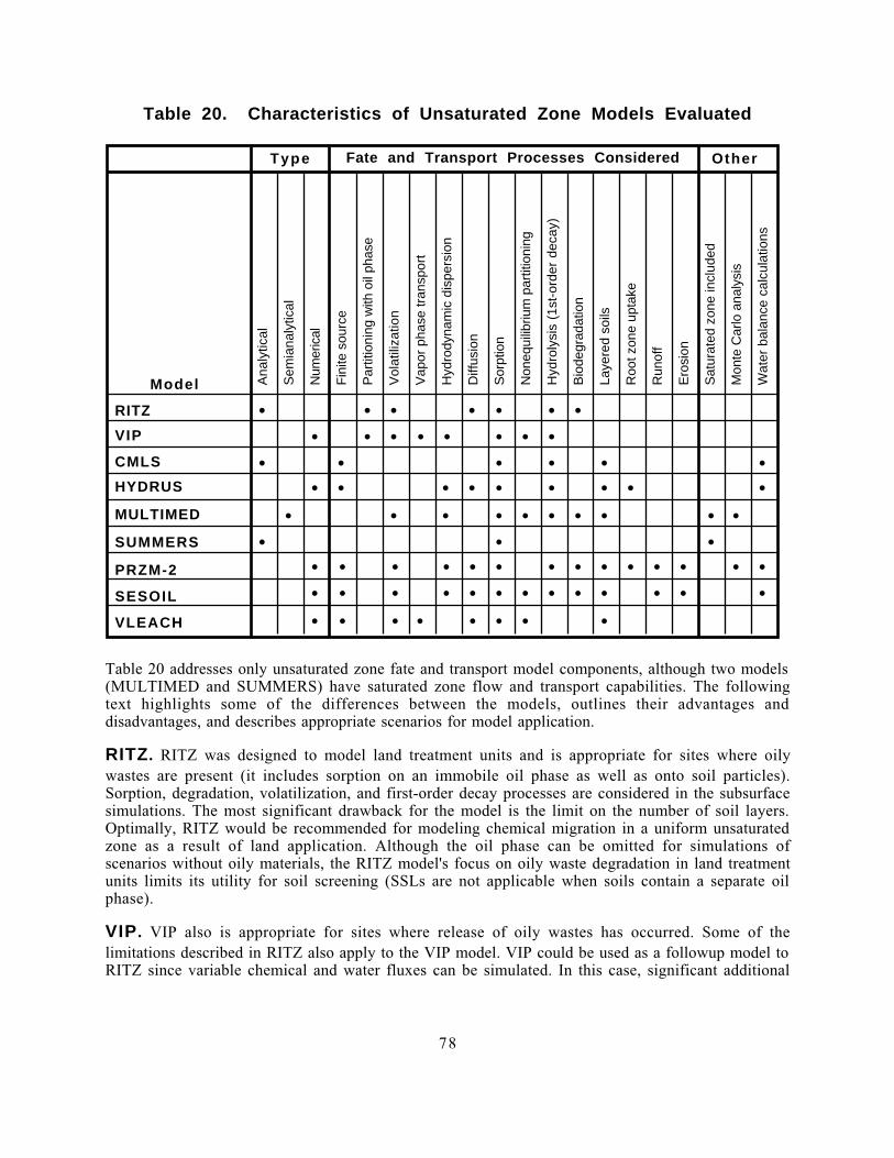
Table 20. Characteristics of Unsaturated Zone Models Evaluated
Sem
iana
lytic
al
Num
eric
al
Fin
ite s
ourc
e
Par
titio
ning
with
oil
phas
e
Vol
atili
zatio
n
Vap
or p
hase
tran
spor
t
Hyd
rody
nam
ic d
ispe
rsio
n
Diff
usio
n
Sor
ptio
n
Non
equi
libriu
m p
artit
ioni
ng
Hyd
roly
sis
(1st
-ord
er d
ecay
)
Bio
degr
adat
ion
Laye
red
soils
Roo
t zon
e up
take
Run
off
Ero
sion
Sat
urat
ed z
one
incl
uded
Mon
te C
arlo
ana
lysi
s
Wat
er b
alan
ce c
alcu
latio
ns
Model
RITZ
VIP
CMLS
HYDRUS
MULTIMED
SUMMERS
PRZM-2
SESOIL
VLEACH
Ana
lytic
al
•
•
•
•
•
•
•
•
•
•
•
•
•
•
•
•
•
•
•
•
•
•
•
•
•
•
•
•
•
•
•
•
•
•
•
•
•
•
•
•
•
•
•
•
•
•
•
•
•
•
•
•
•
•
•
•
•
•
•
•
•
•
•
•
•
•
•
•
•
•
•
•
•
•
•
•
•
•
Type
Fate and Transport Processes Considered
Other
Table 20 addresses only unsaturated zone fate and transport model components, although two models(MULTIMED and SUMMERS) have saturated zone flow and transport capabilities. The followingtext highlights some of the differences between the models, outlines their advantages anddisadvantages, and describes appropriate scenarios for model application.
RITZ. RITZ was designed to model land treatment units and is appropriate for sites where oilywastes are present (it includes sorption on an immobile oil phase as well as onto soil particles).Sorption, degradation, volatilization, and first-order decay processes are considered in the subsurfacesimulations. The most significant drawback for the model is the limit on the number of soil layers.Optimally, RITZ would be recommended for modeling chemical migration in a uniform unsaturatedzone as a result of land application. Although the oil phase can be omitted for simulations ofscenarios without oily materials, the RITZ model's focus on oily waste degradation in land treatmentunits limits its utility for soil screening (SSLs are not applicable when soils contain a separate oilphase).
VIP . VIP also is appropriate for sites where release of oily wastes has occurred. Some of thelimitations described in RITZ also apply to the VIP model. VIP could be used as a followup model toRITZ since variable chemical and water fluxes can be simulated. In this case, significant additional
78

input parameters are required to simulate transient partitioning between the air, soil, water, and oilphases. Like RITZ, VIP's focus on land treatment of oily waste limits its application to SSLs.
CMLS. CMLS differs from RITZ and VIP in that it allows designation of up to 20 soil layers withdifferent properties. It does not consider nonaqueous phase liquids, dispersion, diffusion, or vaporphase transport, but a finite source can be modeled. CMLS estimates the location of the peakconcentration of contaminants through a layered soil system. A limitation of the CMLS model forSSL application is that it does not calculate leachate concentrations. Instead, it calculates the amountof chemical at a certain depth at a certain time. The user must estimate the concentration based onthe amount of chemical present and the total flux of water in the system (Nofziger et al., 1994). Themodel is typically used to estimate the time for a chemical entering the unsaturated zone to reach acertain depth.
HYDRUS. Like CMLS, the HYDRUS model can also simulate chemical movement in layered soilsand can consider a finite source, but also includes dispersion and diffusion as well as sorption and first-order decay. In addition, HYDRUS outputs the chemical concentration in the soil water as a functionof time and depth along with the amount of chemical remaining in the soil. The model considers rootzone uptake, but other models such as PRZM should be used if the comprehensive effects of plantuptake are to be considered in the simulations. Because it can estimate infiltration from rainfallcontaminant concentrations, HYDRUS may be useful in SSL applications.
SUMMERS. The SUMMERS model is a relatively simple model designed to simulate leaching inthe unsaturated zone and is essentially identical to the SSL migration to ground water equations inassumptions and limitations. It is appropriate for use as an initial screening model where site data arelimited and where volatilization is not of concern. However, since attenuation processes such asbiodegradation, first-order decay, volatilization, or other attenuation processes (other than sorption)are not considered, it is a quite conservative model. Since volatilization is not considered, it cannotbe used to simulate migration of volatile compounds to the atmosphere. Because of its similarities tothe SSL migration to ground water equations, the SUMMERS model is not suitable for a more detailedassessment of site conditions.
MULTIMED . MULTIMED simulates simple vertical water movement in the unsaturated zone.Since an initial soil concentration cannot be specified, either the soil/water partition equation or aleaching test (SPLP) must be used to estimate soil leachate contaminant concentrations.MULTIMED is appropriate for simulating contaminant migration in soil and can be used to modelvadose zone attenuation of leachate concentrations derived from a partition equation (see Section2.5.1). In addition, since it links the output from the unsaturated zone transport module with asaturated zone module, it can be used to determine the concentration of a contaminant in a welllocated downgradient from a contaminant source. MULTIMED is appropriate for early-stage sitesimulations because the input parameters required are typically available and uncertainty analyses canbe performed using Monte Carlo simulations for those parameters for which reliable values are notknown.
VLEACH. In VLEACH, biological or chemical degradation is not considered. It therefore providesconservative estimates of contaminant migration in soil. This model may be appropriate as an initialscreening tool for sites for which there is little information available. VLEACH can estimate volatileemissions (see Section 3.1) and can consider a finite source. It is therefore potentially applicable toboth subsurface pathways addressed by the soil screening process.
79

SESOIL. SESOIL was designed as a screening tool, but it is actually more complex than some ofthe models described. Some of the input data would be cumbersome to obtain, especially for use as aninitial screening tool. It is applicable for simulating spill sites since it allows consideration of surfacetransport by erosion and runoff and can utilize detailed meteorologic information to estimateinfiltration. In the soil zone, several fate and transport options are available such as metalcomplexation, hydrolysis, cation exchange, and degradation. This model is especially applicable tosites where significant subsurface and meteorologic information is available. Although the model doesconsider volatilization from surface soils, the available documentation (Criscenti et al., 1994) is notclear as to whether it produces an output of volatile flux to the atmosphere.
PRZM-2. PRZM-2 is a relatively detailed model as a result of the coupling of the two modelsPRZM and VADOFT. Although PRZM is predominantly used as a pesticide leaching model, it couldalso be used for simulation of transport of other chemicals. Because detailed meteorology and surfaceapplication parameters can be included, it is appropriate for simulation of surface spills or landdisposal scenarios. In addition, uncertainty analyses can be performed based on Monte Carlosimulations. Numerous subsurface fate and transport options exist in PRZM. Water movement issomewhat simplified in PRZM, and it may not be applicable for low-permeability soils (Criscenti etal., 1994). However, water flow simulation is more detailed in the VADOFT module of the PRZM-2program. The combination of these programs makes PRZM-2 a relatively complex model. Thismodel is especially applicable to sites for which significant site and meteorologic data are available.
80

Part 4: MEASURING CONTAMINANT CONCENTRATIONS IN SOIL
The Soil Screening Guidance includes a sampling strategy for implementing the soil screening process.Section 4.1 presents the sampling approach for surface soils. This approach provides a simpledecision rule based on comparing the maximum contaminant concentrations of composite sampleswith surface soil screening levels (the Max test) to determine whether further investigation is neededfor a particular exposure area (EA). In addition, this section presents a more complex strategy (theChen test) that allows the user to design a site-specific quantitative sampling strategy by varyingdecision error limits and soil contaminant variability to optimize the number of samples andcomposites. Section 4.2 provides a subsurface soil sampling strategy for developing SSLs and applyingthe screening procedure for the volatilization and migration to ground water exposure pathways.
Section 4.3 describes the technical details behind the development of the SSL sampling strategy,including analyses and response to public and peer-review comments received on the December 1994draft guidance.
The sampling strategy for the soil screening process is designed to achieve the following objectives:
• Estimate mean concentrations of contaminants of concern forcomparison with SSLs
• Fill in the data gaps in the conceptual site model necessary to developSSLs.
The soils of interest for the first objective differ according to the exposure pathway being addressed.For the direct ingestion, dermal, and fugitive dust pathways, EPA is concerned about surface soils.The sampling goal is to determine average contaminant concentrations of surface soils in exposureareas of concern. For inhalation of volatiles, migration to ground water and, in some cases, plantuptake, subsurface soils are the primary concern. For these pathways, the average contaminantconcentration through each source is the parameter of interest.
The second objective (filling in the data gaps) applies primarily to the inhalation and migration toground water pathways. For these pathways, the source area and depth as well as average soilproperties within the source are needed to calculate the pathway-specific SSLs. Therefore, thesampling strategy needs to address collection of these site-specific data.
Because of the difference in objectives, the sampling strategies for the ingestion pathway and for theinhalation and migration to ground water pathways are addressed separately. If both surface andsubsurface soils are a concern, then surface soils should be sampled first because the results of surfacesoil analyses may help delineate source areas to target for subsurface sampling.
At some sites, a third sampling objective may be appropriate. As discussed in the Soil ScreeningGuidance, SSLs may not be useful at sites where background contaminant levels are above the SSLs.Where sampling information suggests that background contaminant concentrations may be aconcern, background sampling may be necessary. Methods for Evaluating the Attainment of CleanupStandards - Volume 3: Reference-Based Standards for Soil and Solid Media (U.S. EPA, 1994e)provides further information on sampling soils to determine background conditions at a site.
81
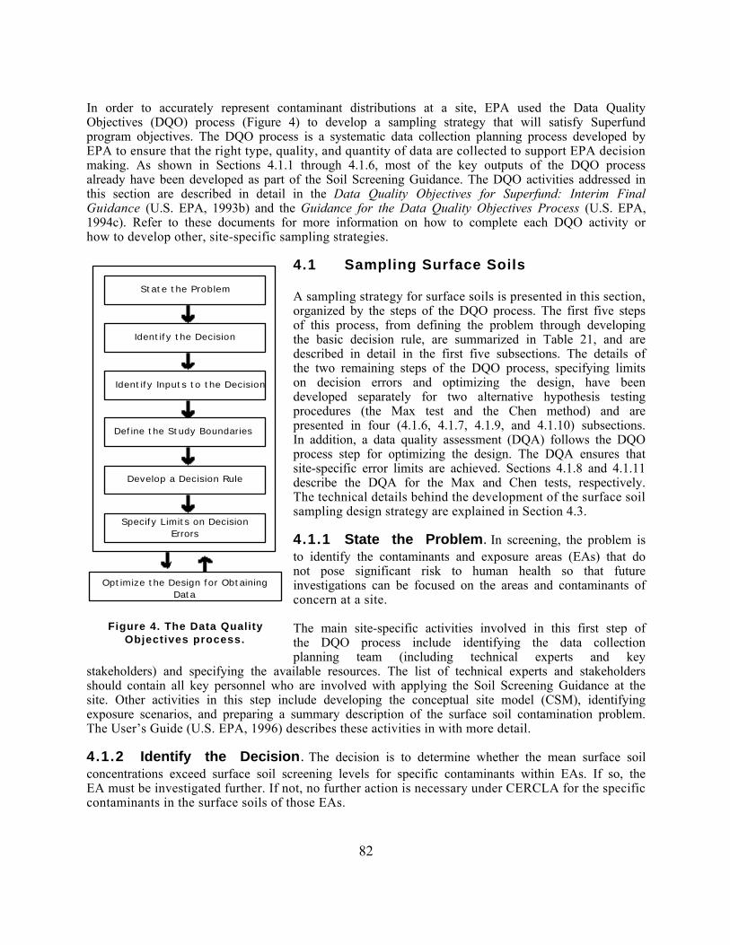
In order to accurately represent contaminant distributions at a site, EPA used the Data QualityObjectives (DQO) process (Figure 4) to develop a sampling strategy that will satisfy Superfundprogram objectives. The DQO process is a systematic data collection planning process developed byEPA to ensure that the right type, quality, and quantity of data are collected to support EPA decisionmaking. As shown in Sections 4.1.1 through 4.1.6, most of the key outputs of the DQO processalready have been developed as part of the Soil Screening Guidance. The DQO activities addressed inthis section are described in detail in the Data Quality Objectives for Superfund: Interim FinalGuidance (U.S. EPA, 1993b) and the Guidance for the Data Quality Objectives Process (U.S. EPA,1994c). Refer to these documents for more information on how to complete each DQO activity orhow to develop other, site-specific sampling strategies.
State the Problem
Identify the Decision
Identify Inputs to the Decision
Define the Study Boundaries
Develop a Decision Rule
Specify Limits on DecisionErrors
Optimize the Design for ObtainingData
Figure 4. The Data QualityObjectives process.
4.1 Sampling Surface Soils
A sampling strategy for surface soils is presented in this section,organized by the steps of the DQO process. The first five stepsof this process, from defining the problem through developingthe basic decision rule, are summarized in Table 21, and aredescribed in detail in the first five subsections. The details ofthe two remaining steps of the DQO process, specifying limitson decision errors and optimizing the design, have beendeveloped separately for two alternative hypothesis testingprocedures (the Max test and the Chen method) and arepresented in four (4.1.6, 4.1.7, 4.1.9, and 4.1.10) subsections.In addition, a data quality assessment (DQA) follows the DQOprocess step for optimizing the design. The DQA ensures thatsite-specific error limits are achieved. Sections 4.1.8 and 4.1.11describe the DQA for the Max and Chen tests, respectively.The technical details behind the development of the surface soilsampling design strategy are explained in Section 4.3.
4.1.1 State the Problem. In screening, the problem isto identify the contaminants and exposure areas (EAs) that donot pose significant risk to human health so that futureinvestigations can be focused on the areas and contaminants ofconcern at a site.
The main site-specific activities involved in this first step ofthe DQO process include identifying the data collectionplanning team (including technical experts and key
stakeholders) and specifying the available resources. The list of technical experts and stakeholdersshould contain all key personnel who are involved with applying the Soil Screening Guidance at thesite. Other activities in this step include developing the conceptual site model (CSM), identifyingexposure scenarios, and preparing a summary description of the surface soil contamination problem.The User’s Guide (U.S. EPA, 1996) describes these activities in with more detail.
4.1.2 Identify the Decision. The decision is to determine whether the mean surface soilconcentrations exceed surface soil screening levels for specific contaminants within EAs. If so, theEA must be investigated further. If not, no further action is necessary under CERCLA for the specificcontaminants in the surface soils of those EAs.
82

Table 21. Sampling Soil Screening DQOs for Surface Soils
DQO Process Steps Soil Screening Inputs/Outputs
State the Problem
Identify scoping team Site manager and technical experts (e.g., toxicologists, risk assessors,statisticians, soil scientists)
Develop conceptual site model (CSM) CSM development (described in Step 1 of the User’s Guide, U.S. EPA, 1996)
Define exposure scenarios Direct ingestion and inhalation of fugitive particulates in a residential setting;dermal contact and plant uptake for certain contaminants
Specify available resources Sampling and analysis budget, scheduling constraints, and availablepersonnel
Write brief summary of contaminationproblem
Summary of the surface soil contamination problem to be investigated at thesite
Identify the Decision
Identify decision Do mean soil concentrations for particular contaminants (e.g., contaminants ofpotential concern) exceed appropriate screening levels?
Identify alternative actions Eliminate area from further study under CERCLAorPlan and conduct further investigation
Identify Inputs to the Decision
Identify inputs Ingestion and particulate inhalation SSLs for specified contaminantsMeasurements of surface soil contaminant concentration
Define basis for screening Soil Screening Guidance
Identify analytical methods Feasible analytical methods (both field and laboratory) consistent withprogram-level requirements
Define the Study Boundaries
Define geographic areas of fieldinvestigation
The entire NPL site (which may include areas beyond facility boundaries),except for any areas with clear evidence that no contamination has occurred
Define population of interest Surface soils (usually the top 2 centimeters, but may be deeper whereactivities could redistribute subsurface soils to the surface)
Divide site into strata Strata may be defined so that contaminant concentrations are likely to berelatively homogeneous within each stratum based on the CSM and fieldmeasurements
Define scale of decision making Exposure areas (EAs) no larger than 0.5 acre each (based on residential landuse)
Define temporal boundaries of study Temporal constraints on scheduling field visits
Identify practical constraints Potential impediments to sample collection, such as access, health, andsafety issues
Develop a Decision Rule
Specify parameter of interest “True mean” (µ) individual contaminant concentration in each EA. (since thedetermination of the “true mean” would require the collection and analysis ofmany samples, the “Max Test” uses another sample statistic, the maximumcomposite concentration).
Specify screening level Screening levels calculated using available parameters and site data (orgeneric SSLs if site data are unavailable).
Specify "if..., then..." decision rule If the “true mean” EA concentration exceeds the screening level, theninvestigate the EA further. If the “true mean” is less than the screeninglevel, then no further investigation of the EA is required under CERCLA.
83

4.1.3 Identify Inputs to the Decision. This step of the DQO process requiresidentifying the inputs to the decision process, including the basis for further investigation and theapplicable analytical methods. The inputs for deciding whether to investigate further are theingestion, dermal, and fugitive dust inhalation SSLs calculated for the site contaminants as describedin Part 2 of this document, and the surface soil concentration measurements for those samecontaminants. Therefore, the remaining task is to identify Contract Laboratory Program (CLP)methods and/or field methods for which the quantitation limits (QLs) are less than the SSLs. EPArecommends the use of field methods, such as soil gas surveys, immunoassays, or X-ray fluorescence,where applicable and appropriate as long as quantitation limits are below the SSLs. At least 10percent of field samples should be split and sent to a CLP laboratory for confirmatory analysis (U.S.EPA, 1993d).
4.1.4 Define the Study Boundaries. This step of the DQO process defines the samplepopulation of interest, subdivides the site into appropriate exposure areas, and specifies temporal orpractical constraints on the data collection. The description of the population of interest mustinclude the surface soil depth.
Sampling Depth. When measuring soil contamination levels at the surface for the ingestionand inhalation pathways, the top 2 centimeters is usually considered surface soil, as defined by UrbanSoil Lead Abatement Project (U.S. EPA 1993f). However, additional sampling beyond this depthmay be appropriate for surface soils under a future residential use scenario in areas where major soildisturbances can reasonably be expected as a result of landscaping, gardening, or constructionactivities. In this situation, contaminants that were at depth can be moved to the surface. Thus, it isimportant to be cognizant of local residential construction practices when determining the depth ofsurface soil sampling and to weigh the likelihood of that area being developed.
Subdividing the Site. This step involves dividing the site into areas or strata depending onthe likelihood of contamination and identifying areas with similar contaminant patterns. Thesedivisions can be based on process knowledge, operational units, historical records, and/or priorsampling. Partitioning the site into such areas and strata can lead to a more efficient sampling designfor the entire site.
For example, the site manager may have documentation that large areas of the site are unlikely tohave been used for waste disposal activities. These areas would be expected to exhibit relatively lowvariability and the sampling design could involve a relatively small number of samples. The greatestintensity of sampling effort would be expected to focus on areas of the site where there is greateruncertainty or greater variability associated with contamination patterns. When relatively largevariability in contaminant concentrations is expected, more samples are required to determine withconfidence whether the EA should be screened out or investigated further.
Initially, the site may be partitioned into three types of areas:
1. Areas that are not likely to be contaminated2. Areas that are known to be highly contaminated3. Areas that are suspected to be contaminated and cannot be ruled out.
Areas that are not likely to be contaminated generally will not require further investigation if thisassumption is based on historical site use information or other site data that are reasonably completeand accurate. (However, the site manager may also want take a few samples to confirm thisassumption). These may be parts of the site that are within the legal boundaries of the property but
84

were completely undisturbed by hazardous-waste-generating activities. All other areas needinvestigation.
Areas that are known to be highly contaminated (i.e., sources) are targeted for subsurface sampling.The information collected on source area and depth is used to calculate site-specific SSLs for theinhalation and migration to ground water pathways (see Section 4.2 for more information).
Areas that are suspected to be contaminated (and cannot be ruled out for screening) are the primarysubjects of the surface soil investigation. If a geostatistician is available, a geostatistical model may beused to characterize these areas (e.g., kriging model). However, guidance for this type of design isbeyond the scope of the current guidance (see Chapter 10 of U.S. EPA, 1989a).
Defining Exposure Areas. After the site has been partitioned into relatively homogeneousareas, each region that is targeted for surface soil sampling is then subdivided into EAs. An EA isdefined as that geographical area in which an individual may be exposed to contamination over time.Because the SSLs were developed for a residential scenario, EPA assumes the EA is a suburbanresidential lot corresponding to 0.5 acre. For soil screening purposes, each EA should be 0.5 acre orless. To the extent possible, EAs should be constructed as square or rectangular areas that can besubdivided into squares to facilitate compositing and grid sampling. If the site is currently residential,then the EA should be the actual residential lot size. The exposure areas should not be laid out in sucha way that they unnecessarily combine areas of high and low levels of contamination. Theorientation and exact location of the EA, relative to the distribution of the contaminant in the soil,can lead to instances where sampling of the EA may lead to results above the mean, and otherinstances, to results below the mean. Try to avoid straddling contaminant “distribution units” withinthe 0.5 acre EA.
The sampling strategy for surface soils allows investigators to determine mean soil contaminantconcentration across an EA of interest. An arithmetic mean concentration for an EA best representsthe exposure to site contaminants over a long period of time. For risk assessment purposes, anindividual is assumed to move randomly across an EA over time, spending equivalent amounts oftime in each location. Since reliable information about specific patterns of nonrandom activity forfuture use scenarios is not available, random exposure appears to be the most reasonable assumptionfor a residential exposure scenario. Therefore, spatially averaged surface soil concentrations are usedto estimate mean exposure concentrations.
Because all the EAs within a given stratum should exhibit similar contaminant concentrations, onesite-specific sampling design can be developed for all EAs within that stratum. As discussed above,some strata may have relatively low variability and other strata may have relatively high variability.Consequently, a different sampling design may be necessary for each stratum, based upon thestratum-specific estimate of the contaminant variability.
4.1.5 Develop a Decision Rule. Ideally, the decision rule for surface soils is:
If the mean contaminant concentration within an EA exceeds the screening level,then investigate that EA further.
This "screening level" is the actual numerical value used to compare against the site contaminationdata. It may be identical to the SSL, or it may be a multiple of the SSL (e.g., 2 SSL) for a hypothesistest designed to achieve specified decision error rates in a specified region above and below the SSL.In addition, another sample statistic (e.g., the maximum concentration) may be used as an estimateof the mean for comparison with the "screening level."
85

4.1.6 Specify Limits on Decision Errors for the Max Test. Sampling data will beused to support a decision about whether an EA requires further investigation. Because of variabilityin contaminant concentrations within an EA, practical constraints on sample sizes, and sampling ormeasurement error, the data collected may be inaccurate or nonrepresentative and may mislead thedecision maker into making an incorrect decision. A decision error occurs when sampling datamislead the decision maker into choosing a course of action that is different from or less desirablethan the course of action that would have been chosen with perfect information (i.e., with noconstraints on sample size and no measurement error).
EPA recognizes that data obtained from sampling and analysis are never perfectly representative andaccurate, and that the costs of trying to achieve near-perfect results can outweigh the benefits.Consequently, EPA acknowledges that uncertainty in data must be tolerated to some degree. TheDQO process controls the degree to which uncertainty in data affects the outcomes of decisions thatare based on those data. This step of the DQO process allows the decision maker to set limits on theprobabilities of making an incorrect decision.
The DQO process utilizes hypothesis tests to control decision errors. When performing a hypothesistest, a presumed or baseline condition, referred to as the "null hypothesis" (Ho), is established. Thisbaseline condition is presumed to be true unless the data conclusively demonstrate otherwise, which iscalled "rejecting the null hypothesis" in favor of an alternative hypothesis. For the Soil ScreeningGuidance, the baseline condition, or Ho, is that the site needs further investigation.
When the hypothesis test is performed, two possible decision errors may occur:
1. Decide not to investigate an EA further (i.e., "walk away") when the correct decision(with complete and perfect information) would be to "investigate further"
2. Decide to investigate further when the correct decision would be to "walk away."
Since the site is on the NPL, site areas are presumed to need further investigation. Therefore, thedata must provide clear evidence that it would be acceptable to "walk away." This presumptionprovides the basis for classifying the two types of decision errors. The "incorrectly walk away"decision error is designated as the Type I decision error because one has incorrectly rejected thebaseline condition (null hypothesis). Correspondingly, the "unnecessarily investigate further"decision error is designated as the Type II decision error.
To complete the specification of limits on decision errors, Type I and Type II decision errorprobability limits must be defined in relation to the SSL. First a "gray region" is specified with respectto the mean contaminant concentration within an EA. The gray region represents the range ofcontaminant levels near the SSL, where uncertainty in the data (i.e., the variability) can make thedecision "too close to call." In other words, when the average of the data values is very close to theSSL, it would be too expensive to generate a data set of sufficient size and precision to resolve whatthe correct determination should be. (i.e., Does the average concentration fall "above" or "below"the SSL?)
The Soil Screening Guidance establishes a default range for the width and location of the "grayregion": from one-half the SSL (0.5 SSL) to two times the SSL (2 SSL). By specifying the upper edgeof the gray region as twice the SSL, it is possible that exposure areas with mean values slightly higherthan the SSL may be screened from further study. However, EPA believes that the exposure scenario
86

and assumptions used to derive SSLs are sufficiently conservative to be protective in such cases.
On the lower side of the gray region, the consequences of decision errors at one-half the SSL areprimarily financial. If the lower edge of the gray region were to be moved closer to the SSL, thenmore exposure areas that were truly below the SSL would be screened out, but more money would bespent on sampling to make this determination. If the lower edge of the gray region were to be movedcloser to zero, then less money could be spent on sampling, but fewer EAs that were truly below theSSLs would be screened out, leading to unnecessary investigation of EAs. The Superfund programchose the gray region to be one-half to two times the SSL after investigating several different ranges.This range for the gray region represents a balance between the costs of collecting and analyzing soilsamples and making incorrect decisions. While it is desirable to estimate exactly the exposure areamean, the number of samples required are much more than project managers are generally willing tocollect in a "screening" effort. Although some exposure areas will have contaminant concentrationsthat are between the SSL and twice the SSL and will be screened out, human health will still beprotected given the conservative assumptions used to derive the SSLs.
The Soil Screening Guidance establishes the following goals for Type I and Type II decision errorrates:
• Prob ("walk away" when the true EA mean is 2 SSL) = 0.05• Prob ("investigate further" when the true EA mean is 0.5 SSL) = 0.20.
This means that there should be no more than a 5 percent chance that the site manager will "walkaway" from an EA where the true mean concentration is 2 SSL or more. In addition, there should beno more than a 20 percent chance that the site manager will unnecessarily investigate an EA whenthe mean is 0.5 SSL or less.
These decision error limits are general goals for the soil screening process. Consistent with the DQOprocess, these goals may be adjusted on a site-specific basis by considering the available resources(i.e., time and budget), the importance of screening surface soil relative to other potential exposurepathways, consequences of potential decision errors, and consistency with other relevant EPAguidance and programs.
Table 22 summarizes this step of the DQO process for the Max test, specifying limits on the decisionerror rates, and the final step of the DQO process for the Max test, optimizing the design. Figure 5illustrates the gray region for the decision error goals: a Type I decision error rate of 0.05 (5percent) at 2 SSL and a Type II decision error rate of 0.20 (20 percent) at 0.5 SSL.
4.1.7 Optimize the Design for the Max Test. This section provides instructions fordeveloping an optimum sampling strategy for screening surface soils. It discusses compositing, theselection of sampling points for composited and uncomposited surface soil sampling, and therecommended procedures for determining the sample sizes necessary to achieve specified limits ondecision errors using the Max test.
87

Table 22. Sampling Soil Screening DQOs for Surface Soils under theMax Test
DQO Process Steps Soil Screening Inputs/Outputs
Specify Limits on Decision Errors*
Define baseline condition (nullhypothesis)
The EA needs further investigation
Define the gray region** From 0.5 SSL to 2 SSL
Define Type I and Type II decision errors Type I error: Do not investigate further ("walk away from") an EA whose truemean exceeds the screening level of 2 SSLType II error: Investigate further when an EA's true mean falls below thescreening level of 0.5 SSL
Identify consequences Type I error: potential public health consequencesType II error: unnecessary expenditure of resources to investigate further
Assign acceptable probabilities of Type Iand Type II decision errors
Goals:Type I: 0.05 (5%) probability of not investigating further when “true mean” of
the EA is 2 SSLType II: 0.20 (20%) probability of investigating further when “true mean” of
the EA is 0.5 SSL
Define QA/QC goals CLP precision and bias requirements10% CLP analyses for field methods
Optimize the Design
Determine how to best estimate “truemean”
Samples composited across the EA estimate the EA mean (− x ). Use maximum
composite concentration as a conservative estimate of the true EA mean.
Determine expected variability of EAsurface soil contaminant concentrations
A conservatively large expected coefficient of variation (CV) from prior datafor the site, field measurements, or data from other comparable sites andexpert judgment. A minimum default CV of 2.5 should be used wheninformation is insufficient to estimate the CV.
Design sampling strategy by evaluatingcosts and performance of alternatives
Lowest cost sampling design option (i.e., compositing scheme and number ofcomposites) that will achieve acceptable decision error rates
Develop planning documents for the fieldinvestigation
Sampling and Analysis Plan (SAP)Quality Assurance Project Plan (QAPjP)
* Since the DQO process controls the degree to which uncertainty in data affects the outcome of decisions that arebased on that data, specifying limits on decision errors will allow the decision maker to control the probability of makingan incorrect decision when using the DQOs.
** The gray region represents the area where the consequences of decision errors are minor (and uncertainty in samplingdata makes decisions too close to call).
88

1.0
_ 0.9
_ 0.8
_ 0.7
_ 0.6
_ 0.5
_ 0.4
_ 0.3
_ 0.2
_ 0.1
0
1.0
0.9 _
0.8 _
0.7 _
0.6 _
0.5 _
0.4 _
0.3 _
0.2 _
0.1 _
0
Probability ofDeciding that
the MeanExceeds the
Screening LevelGray Region
(Relatively LargeDecision Error Rates
are ConsideredTolerable.)
0.95
0.5 H SSL SSL 2 H SSL
True Mean Contaminant Concentration
TolerableType IIDecisionErrorRates
Tolerable Type IDecision Error
Rates
Figure 5. Design performance goal diagram.
Note that the size, shape, and orientation of sampling volume (i.e., “support”) for heterogenousmedia have a significant effect on reported measurement values. For instance, particle size has avarying affect on the transport and fate of contaminants in the environment and on the potentialreceptors. Because comparison of data from methods that are based on different supports can bedifficult, defining the sampling support is important in the early stages of site characterization. Thismay be accomplished through the DQO process with existing knowledge of the site, contamination,and identification of the exposure pathways that need to be characterized. Refer to Preparation ofSoil Sampling Protocols: Sampling Techniques and Strategies (U.S. EPA, 1992f) for moreinformation about soil sampling support.
The SAP developed for surface soils should specify sampling and analytical procedures as well as thedevelopment of QA/QC procedures. To identify the appropriate analytical procedures, the screeninglevels must be known. If data are not available to calculate site-specific SSLs, then the generic SSLs inAppendix A should be used.
Compositing. Because the objective of surface soil screening is to ensure that the meancontaminant concentration does not exceed the screening level, the physical "averaging" that occursduring compositing is consistent with the intended use of the data. Compositing allows a largernumber of locations to be sampled while controlling analytical costs because several discrete samplesare physically mixed (homogenized) and one or more subsamples are drawn from the mixture andsubmitted for analysis. If the individual samples in each composite are taken across the EA, eachcomposite represents an estimate of the EA mean.
A practical constraint to compositing in some situations is the heterogeneity of the soil matrix. The
89

efficiency and effectiveness of the mixing process may be hindered when soil particle sizes varywidely or when the soil matrix contains foreign objects, organic matter, viscous fluids, or stickymaterial. Soil samples should not be composited if matrix interference among contaminants is likely(e.g., when the presence of one contaminant biases analytical results for another).
Before individual specimens are composited for chemical analysis, the site manager should considerhomogenizing and splitting each specimen. By compositing one portion of each specimen with theother specimens and storing one portion for potential future analysis, the spatial integrity of eachspecimen is maintained. If the concentration of a contaminant in a composite sample is high, thesplits of the individual specimens from which it was composed can be analyzed discretely todetermine which individual specimen(s) have high concentrations of the contaminant. This willpermit the site manager to determine which portion within an EA is contaminated without making arepeat visit to the site.
Sample Pattern. The Max test should only be applied using composite samples that arerepresentative of the entire EA. However, the Chen test (see Section 4.1.9) can be applied withindividual, uncomposited samples. There are several options for developing a sampling pattern forcompositing that produce samples that should be representative. If individual, uncomposited sampleswill be analyzed for contaminant concentrations, the N sample points can be selected using either (1)simple random sampling (SRS), (2) stratified SRS, or (3) systematic grid sampling (square orrectangular grid) with a random starting point (SyGS/rs). Step-by-step procedures for selecting SRSand SyGS/rs samples are provided in Chapter 5 of the U.S. EPA (1989a) and Chapter 5 of U.S. EPA(1994e). If stratified random sampling is used, the sampling rate must be the same in every sector, orstratum of the EA. Hence, the number of sampling points assigned to a stratum must be directlyproportional to the surface area of the stratum.
Systematic grid sampling with a random starting point is generally preferred because it ensures thatthe sample points will be dispersed across the entire EA. However, if the boundaries of the EA areirregular (e.g., around the perimeter of the site or the boundaries of a stratum within which the EAswere defined), the number of grid sample points that fall within the EA depends on the randomstarting point selected. Therefore, for these irregularly shaped EAs, SRS or stratified SRS isrecommended. Moreover, if a systematic trend of contamination is suspected across the EA (e.g., astrip of higher contamination), then SRS or stratified SRS is recommended again. In this case, gridsampling would be likely to result in either over- or under representation of the strip of highercontaminant levels, depending on the random starting point.
For composite sampling, the sampling pattern used to locate the discrete sample specimens that formeach composite sample (N) is important. The composite samples should be formed in a manner thatis consistent with the assumptions underlying the sample size calculations. In particular, eachcomposite sample should provide an unbiased estimate of the mean contaminant concentration overthe entire EA. One way to construct a valid composite of C specimens is to divide the EA into Csectors, or strata, of equal area and select one point at random from each sector. If sectors (strata)are of unequal sizes, the simple average is no longer representative of the EA as a whole.
Five valid sampling patterns and compositing schemes for selecting N composite samples that eachconsist of C specimens are listed below:
1. Select an SRS consisting of C points and composite all specimens associated with these pointsinto a sample. Repeat this process N times, discarding any points that were used in a previoussample.
90

2. Select an SyGS/rs of C points and composite all specimens associated with the points in thissample. Repeat this process N times, using a new randomly selected starting point each time.
3. Select a single SyGS/rs of CHN points and use the systematic compositing scheme that isdescribed in Highlight 3 to form N composites, as illustrated in Figure 6.
4. Select a single SyGS/rs of CHN points and use the random compositing scheme that isdescribed in Highlight 4 to form N composites, as illustrated in Figure 7.
5. Select a stratified random sample of CHN points and use a random compositing scheme, asdescribed in Highlight 5, to form N composites, as illustrated in Figure 8.
Methods 1, 2, and 5 are the most statistically defensible, with method 5 used as the default method inthe Soil Screening Guidance. However, given the practical limits of implementing these methods,either method 3 or 4 is generally recommended for EAs with regular boundaries (e.g., square orrectangular). As noted above, if the boundaries of the EA are irregular, SyGS/rs sampling may notresult in exactly CHN sample points. Therefore, for EAs with irregular boundaries, method 5 isrecommended. Alternatively, a combination of methods 4 and 5 can be used for EAs that can bepartitioned into C sectors of equal area of which K have regular boundaries and the remaining C - Khave irregular boundaries.
Additionally, compositing within sectors to indicate whether one sector of the EA exceeds SSLs is anoption that may also be considered. See Section 4.3.6 for a full discussion.
Sample Size. This section presents procedures to determine sample size requirements for theMax test that achieve the site-specific decision error limits discussed in Section 4.1.6. The Max testis based on the maximum concentration observed in N composite samples that each consist of Cindividual specimens. The individual specimens are selected so that each of the N composite samplesis representative of the site as a whole, as discussed above. Hence, this section addresses determiningthe sample size pair, C and N, that achieves the site-specific decision error limits. Directions forperforming the Max test in a manner that is consistent with DQOs established for a site are presentedlater in this section.
Table 23 presents the probabilities of Type I errors at 2 SSL and Type II errors at 0.5 SSL (theboundary points of the gray region discussed in Section 4.1.6) for several sample size options whenthe variability for concentrations of individual measurements across the EA ranges from 100 percentto 400 percent (CV = 1.0 to 4.0). Two choices for the number, C, of specimens per composite areshown in this table: 4 and 6. Fewer than four specimens per composite is not considered sufficient forthe Max test. Fewer than four specimens per composite does not achieve the decision error limitgoals for the level of variability generally encountered at CERCLA sites. More than six specimensmay be more than can be effectively homogenized into a composite sample.
The number, N, of composite samples shown in Table 23 ranges from 4 to 9. Fewer than foursamples is not considered sufficient because, considering decision error rates from simulation results(Section 4.3), the Max text should be based on at least four independent estimates of the EA mean.More than nine composite samples per EA is generally unlikely for screening surface soils atSuperfund sites. However, additional sample size options can be determined from the simulationresults reported in Appendix I.
91

Highlight 3: Procedure for Compositing of Specimens from a Grid Sample Using a Systematic Scheme (Figure 6)
1. Lay out a square or triangular grid sample over the EA, using a random start. Step-by-stepprocedures can be found in Chapter 5 of U.S. EPA (1989a). The number of points in the gridshould be equal to CHN, where C is the desired number of specimens per composite and N is thedesired number of composites.
2. Divide the EA into C sectors (strata) of equal area and shape such that each sector contains thesame number of sample points. The number of sectors (C) should be equal to the number ofspecimens in each composite (since one specimen per area will be used in each composite) andthe number of points within each sector, N, should equal the desired number of compositesamples.
3. Label the points within one sector in any arbitrary fashion from 1 to N. Use the same scheme foreach of the other sectors.
4. Form composite number 1 by compositing specimens with the '1' label, form composite number 2by compositing specimens with the '2' label, etc. This leads to N composite samples that aresubjected to chemical analysis.
l1 l2
l3 l4
l5 l6
l1 l2
l3 l4
l5 l6
l1 l2
l3 l4
l5 l6
l1 l2
l3 l4
l5 l6
Figure 6. Systematic (square grid points) sample with systematic compositing scheme(6 composite samples consisting of 4 specimens).
92

Highlight 4: Procedure for Compositing of Specimens from a Grid Sample Using aRandom Scheme (Figure 7)
1. Lay out a square or triangular grid sample over the EA, using a random start. Step-by-stepprocedures can be found in Chapter 5 of U.S. EPA (1989a). The number of points in the gridshould be equal to CHN, where C is the desired number of specimens per composite and N isthe desired number of composites.
2. Divide the EA into C sectors (strata) of equal area and shape such that each sector containsthe same number of sample points. The number of sectors (C) should be equal to the numberof specimens in each composite (since one specimen per area will be used in eachcomposite) and the number of points within each sector, N, should equal the desired numberof composite samples.
3. Use a random number table or random number generator to establish a set of labels for the Npoints within each sector. This is done by first labeling the points in a sector in an arbitraryfashion (say, points A, B, C,...) and associating the first random number with point A, thesecond with point B, etc. Then rank the points in the sector according to the set of randomnumbers and relabel each point with its rank. Repeat this process for each sector.
4. Form composite number 1 by compositing specimens with the ‘1’ label, form compositenumber 2 by compositing specimens with the ‘2’ label, etc. This leads to N composite samplesthat are subjected to chemical analysis.
l3 l2
l1 l4
l5 l6
l1 l5
l6 l3
l2 l4
l6 l5
l1 l4
l3 l2
l4 l6
l3 l5
l2 l1
Figure 7. Systematic (square grid points) sample with random compositing scheme(6 composite samples consisting of 4 specimens).
93

Highlight 5: Procedure for Compositing of Specimens from a Stratified RandomSample Using a Random Scheme (Figure 8)
1. Divide the EA into C sectors (strata) of equal area, where C is equal to the number ofspecimens to be in each composite (since one specimen per stratum will be used in eachcomposite).
2. Within each stratum, choose N random locations, where N is the desired number ofcomposites. Step-by-step procedures for choosing random locations can be found inChapter 5 of U.S. EPA (1989a).
3. Use a random number table or random number generator to establish a set of labels for the Npoints within each sector. This is done by first labeling the points in a sector in an arbitraryfashion (say, points A, B, C,...) and associating the first random number with point A, thesecond with point B, etc. Then rank the points in the sector according to the set of randomnumbers and relabel each point with its rank. Repeat this process for each sector.
4. Form composite number 1 by compositing specimens with the '1' label, form compositenumber 2 by compositing specimens with the '2' label, etc. This leads to N composite samplesthat are subjected to chemical analysis.
l1
l2
l3
l4
l5
l6
l1
l2
l3
l4
l5
l6
l1
l2
l3
l4
l5
l6
l1
l2
l3
l4
l5
l6
Figure 8. Stratified random sample with random compositing scheme(6 composite samples consisting of 4 specimens).
94

Table 23. Probability of Decision Error at 0.5 SSL and 2 SSL Using Max Test
CV=1.0a CV=1.5 CV=2.0 CV=2.5 CV=3.0 CV=3.5 CV=4.0
SampleSizeb E0.5
c E2.0d E0.5 E2.0 E0.5 E2.0 E0.5 E2.0 E0.5 E2.0 E0.5 E2.0 E0.5 E2.0
C = 4 specimens per compositee
4 <.01 0.08 0.02 0.11 0.09 0.13 0.14 0.19 0.19 0.20 0.24 0.26 0.25 0.30
5 <.01 0.05 0.02 0.06 0.11 0.10 0.15 0.10 0.26 0.17 0.26 0.18 0.31 0.25
6 <.01 0.03 0.02 0.04 0.11 0.06 0.21 0.08 0.28 0.11 0.31 0.11 0.35 0.16
7 <.01 0.01 0.03 0.02 0.12 0.04 0.25 0.05 0.31 0.08 0.36 0.09 0.41 0.15
8 <.01 0.01 0.03 0.01 0.16 0.02 0.25 0.04 0.36 0.05 0.42 0.07 0.41 0.09
9 <.01 0.01 0.05 0.01 0.16 0.01 0.28 0.03 0.36 0.04 0.44 0.07 0.48 0.08
C = 6 specimens per composite
4 <.01 0.08 <.01 0.11 0.03 0.12 0.08 0.16 0.15 0.17 0.26 0.20 0.23 0.27
5 <.01 0.05 <.01 0.06 0.04 0.09 0.11 0.09 0.17 0.13 0.22 0.15 0.25 0.20
6 <.01 0.03 0.01 0.04 0.06 0.04 0.14 0.06 0.19 0.09 0.25 0.09 0.29 0.12
7 <.01 0.01 0.01 0.02 0.06 0.02 0.14 0.04 0.23 0.06 0.29 0.08 0.37 0.08
8 <.01 0.01 0.01 0.01 0.06 0.02 0.15 0.02 0.25 0.03 0.30 0.04 0.40 0.06
9 <.01 0.01 0.01 0.01 0.06 0.01 0.18 0.02 0.28 0.03 0.34 0.03 0.39 0.04
a The CV is the coefficient of variation for individual, uncomposited measurements across the entire EA, including measurement error. b Sample size (N) = number of composite samples. c E0.5 = Probability of requiring further investigation when the EA mean is 0.5 SSL. d E2.0 = Probability of not requiring further investigation when the EA mean is 2.0 SSL. e C = number of specimens per composite sample, where each composite consists of points from a stratified random or systematic grid sample from across the
entire EA. NOTE: All decision error rates are based on 1,000 simulations that assume that each composite is representative of the entire EA, that half the EA has
concentrations below the quantitation limit (i.e., SSL/100), and half the EA has concentrations that follow a gamma distribution (a conservativedistributional assumption).
95

The error rates shown in Table 23 are based on the simulations presented in Appendix I. Thesesimulations are based on the following assumptions:
1. Each of the N composite samples is based on C specimens selected to berepresentative of the EA as a whole, as specified above (C = number of sectors orstrata).
2. One-half the EA has concentrations below the quantitation limit (which is assumed tobe SSL/100).
3. One-half the EA has concentrations that follow a gamma distribution (see Section 4.3for additional discussion).
4. Each chemical analysis is subject to a 20 percent measurement error.
The error rates presented in Table 23 are based on the above assumptions which make them robustfor most potential distributions of soil contaminant concentrations. Distribution assumptions 2 and 3were used because they were found in the simulations to produce high error rates relative to otherpotential contaminant distributions (see Section 4.3). If the proportion of the site below thequantitation limit (QL) is less than half or if the distribution of the concentration measurements issome other distribution skewed to the right (e.g., lognormal), rather than gamma, then the error ratesachieved are likely to be no worse than those cited in Table 23. Although the actual contaminantdistribution may be different from those cited above as the basis for Table 23, only extensiveinvestigations will usually generate sufficient data to determine the actual distribution for each EA.
Using Table 23 to determine the sample size pair (C and N) needed to achieve satisfactory error rateswith the Max test requires an a priori estimate of the coefficient of variation for measurements ofthe contaminant of interest across the EA. The coefficient of variation (CV) is the ratio of thestandard deviation of contaminant concentrations for individual, uncomposited specimens divided bythe EA mean concentration. As discussed in Section 4.1.4, the EAs should be constructed withinstrata expected to have relatively homogeneous concentrations so that an estimate of the CV for astratum may be applicable for all EAs in that stratum. The site manager should use a conservativelylarge estimate of the CV for determining sample size requirements because additional sampling will beneeded if the data suggest that the true CV is greater than that used to determine the sample sizes.
Potential sources of information for estimating the EA or stratum means, variances, and CVs includethe following (in descending order of desirability):
• Data from a pilot study conducted at the site• Prior sampling data from the site• Data from similar sites• Professional judgment.
For more information on estimating variability, see Section 6.3.1 of U.S. EPA (1989a).
4.1.8 Using the DQA Process: Analyzing Max Test Data. This section providesguidance for analyzing the data for the Max test.
The hypothesis test for the Max test is very simple to implement, which is one reason that the Maxtest is attractive as a surface soil screening test. If x1, x2, ..., xN represent concentrationmeasurements for N composite samples that each consist of C specimens selected so that each
96
composite is representative of the EA as a whole (as described in Section 4.1.7), the Max test isimplemented as follows:
If Max (x1, x2, ..., xN) $ 2 SSL, then investigate the EA further; If Max (x1, x2, ..., xN) < 2 SSL, and the data quality assessment (DQA) indicates that thesample size was adequate, then no further investigation is necessary.
In addition, the step-by-step procedures presented in Highlight 6 must be implemented to ensure thatthe site-specific error limits, as discussed in Section 4.1.6, are achieved.
If the EA mean is below 2 SSL, the DQA process may be used to determine if the sample size wassufficiently large to justify the decision to not investigate further. To use Table 23 to check whetherthe sample size is adequate, an estimate of the CV is needed for each EA. The first four steps ofHighlight 6, the DQA process for the Max test, present a process for the computation of a sampleCV for an EA based on the N composite samples that each consist of C specimens.
However, the sample CV can be quite large when all the measurements are very small (e.g., well belowthe SSL) because CV approaches infinity as the EA sample mean (− x ) approaches zero. Thus, whenthe composite concentration values for an EA are all near zero, the sample CV may be questionableand therefore unreliable for determining if the original sample size was sufficient (i.e., it could lead tofurther sampling when the EA mean is well below 2 SSL). To protect against unnecessary additionalsampling in such cases, compare all composites against the equation given in Step 5 of Highlight 6. Ifthe maximum composite sample concentration is below the value given by the equation, then thesample size may be assumed to be adequate and no further DQA is necessary.
To develop Step 5, EPA decided that if there were no compositing (C=1) and all the observations(based on a sample size appropriate for a CV of 2.5) were less than the SSL, then one can reasonablyassume that the EA mean was not greater than 2 SSL. Likewise, because the standard error for themean of C specimens, as represented by the composite sample, is proportional to 1/ C , thecomparable condition for composite observations is that one can reasonably assume that the EAmean was not greater than 2 SSL when all composite observations were less than SSL/ C . If this isthe case for an EA sample set, the sample size can be assumed to be adequate and no further DQA isneeded. Otherwise (when at lease one composite observation is not this small), use Table 23 with thesample CV for the EA to determine whether a sufficient number of samples were taken to achieveDQOs.
In addition to being simple to implement, the Max test is recommended because it provides goodcontrol over the Type I error rates at 2 SSL with small sample sizes. It also does not need anyassumptions regarding observations below the QL. Moreover, the Max test error rates at 2 SSL arefairly robust against alternative assumptions regarding the distribution of surface soil concentrationsin the EA. The simulations in Appendix I show that these error rates are rather stable for lognormalor Weibull contaminant concentration distributions and for different assumptions about portions ofthe site with contaminant concentrations below the QL.
97

Highlight 6: Directions for Data Quality Assessment for the Max Test
Let x1, x2, ..., xN represent contaminant concentration measurements for N composite samples thateach consist of C specimens selected so that each composite is representative of the EA as a whole.The following describes the steps required to ensure that the Max test achieves the DQOsestablished for the site.
STEP 1: The site manager determines the Type I error rate to be achieved at 2 SSL and the Type IIerror rate to be achieved at 0.5 SSL, as described in Section 4.1.6.
STEP 2: Calculate the sample mean − x = N
3 i = 1
x i 1 N
STEP 3: Calculate the sample standard deviation
s = 1
N − 1
N
3 i = 1
x i − − x 2
STEP 4: Calculate the sample estimate of the coefficient of variation, CV, for individual concentrationmeasurements from across the EA.
CV = C s− x
NOTE: This is a conservation approximation of the CV for individual measurements.
STEP 5: If Max (x1, x
2, ..., x
N) <
SSL
C , then no further data quality assessment is needed and the EA
needs no further investigation.
Otherwise proceed to Step 6.
STEP 6: Use the value of the sample CV calculated in Step 4 as the true CV of concentrations todetermine which column of Table 23 is applicable for determining sample sizerequirements. Using the error limits established in Step 1, determine the sample sizerequirements from this table. If the required sample size is greater than that implemented,further investigation of the EA is necessary. The further investigation may consist ofselecting a supplemental sample and repeating the Max test with the larger, combinedsample.
A limitation of the Max test is that it does not provide as good control over the Type II error ratesat 0.5 SSL as it does for Type I error rates at 2 SSL. In fact, for a fixed number, C, of specimens percomposite, the Type II error rate increases as the number of composite samples, N, increases. As thesample size increases, the likelihood of observing an unusual sample with the maximum exceeding 2SSL increases. However, the Type II error rate can be decreased by increasing the number of
98
specimens per composite. This unusual performance of the Max test as a hypothesis testingprocedure occurs because the rejection region is fixed below 2 SSL and thus does not depend on thesample size (as it does for typical hypothesis testing procedures).
4.1.9 Specify Limits on Decision Errors for Chen Test. Although the Max test isadequate and appropriate for selecting a sample size for site screening, there are other alternatemethods of screening surface soils. One such alternate method is the Chen test. In general, the Chentest differs from the Max test in its basic assumption about site contamination and the purpose ofsoil sampling. Because of this variation, these two methods have different null hypotheses anddifferent decision error types.
There are two formulations of the statistical hypothesis test concerning the true (but unknown)mean contaminant concentration, µ, that achieve the Soil Screening Guidance decision error rategoals specified in Section 4.1.6. They are:
1. Test the null hypothesis, H0: µ ≥ 2 SSL, versus the alternative hypothesis,H1: µ < 2 SSL, at the 5 percent significance level using a sample size chosen toachieve a Type II error rate of 20 percent at 0.5 SSL.
2. Test the null hypothesis, H0: µ ≤ 0.5 SSL, versus the alternative hypothesis,H1: µ > 0.5 SSL, at the 20 percent significance level using a sample size chosen toachieve a Type II error rate of 5 percent at 2 SSL.
The first formulation of the problem (which is commonly used in the Superfund program) has theadvantage that the error rate that has potential public health consequences is controlled directly viathe significance level of the test. The error rate that has primarily cost consequences can be reducedby increasing the sample size above the minimum requirement. However, EPA has identified a newtest procedure, the Chen test (Chen, 1995), which requires the second formulation but is less sensitiveto assumptions regarding the distribution of the contaminant measurements than the Land procedureused in the December 1994 draft Technical Background Document (see Section 4.3). This sectionprovides guidance regarding application of the Chen test and is, therefore, based on the secondformulation of the hypothesis test.
A disadvantage of the second formulation is its performance when the true EA mean is between 0.5SSL and the SSL. In this case, as the sample size increases, the test indicates the decision toinvestigate further, even though the mean is less than the SSL. In fact, no test procedure with feasiblesample sizes performs well when the true EA mean is in the "gray region" between 0.5 SSL and 2 SSL(see Section 4.3). Whenever large sample sizes are feasible, one should modify the problem statementand test the null hypothesis, H0: µ ≤ SSL, instead of H0: µ ≤ 0.5 SSL. One would then developappropriate DQOs for this modified hypothesis test (e.g., significance level of 20 percent at the SSLand 5 percent probability of decision error at 2 SSL).
When the true mean of an EA is compared with the screening level, there are two possible decisionerrors that may occur: (1) decide not to investigate an EA further (i.e., "walk away") when thecorrect decision would be to "investigate further"; and (2) decide to investigate further when thecorrect decision would be to "walk away." For the Chen test, the "incorrectly walk away" decisionerror is designated as the Type II decision error because it occurs when we incorrectly accept the nullhypothesis. Correspondingly, the "unnecessarily investigate further" decision error is designated asthe Type I decision error because it occurs when we incorrectly reject the null hypothesis.
99

As discussed in Section 4.1.6, the Soil Screening Guidance specifies a default gray region for decisionerrors from 0.5 SSL to 2 SSL and sets the following goals for Type I and Type II error rates:
• Prob ("investigate further" when the true EA mean is 0.5 SSL) = 0.20• Prob ("walk away" when the true EA mean is 2 SSL) = 0.05.
Table 24 summarizes this step of the DQO process for the Chen test, specifying limits on thedecision error rates, and the final step of the DQO process, optimizing the design.
4.1.10 Optimize the Design Using the Chen Test. This section includes guidance ondeveloping an optimum sampling strategy for screening surface soils. It discusses compositing, theselection of sampling points for composited and uncomposited surface soil sampling, and therecommended procedures for determining the sample sizes necessary to achieve specified limits ondecision errors using the Chen test.
Note that the size, shape, and orientation of sampling volume (i.e., “support”) for heterogenousmedia have a significant effect on reported measurement values. For instance, particle size has avarying affect on the transport and fate of contaminants in the environment and on the potentialreceptors. Because comparison of data from methods that are based on different supports can bedifficult, defining the sampling support is important in the early stages of site characterization. Thismay be accomplished through the DQO process with existing knowledge of the site, contamination,and identification of the exposure pathways that need to be characterized. Refer to Preparation ofSoil Sampling Protocols: Sampling Techniques and Strategies (U.S. EPA, 1992f) for moreinformation about soil sampling support.
The SAP developed for surface soils should specify sampling and analytical procedures as well as thedevelopment of QA/QC procedures. To identify the appropriate analytical procedures, the screeninglevels must be known. If data are not available to calculate site-specific SSLs, then the generic SSLs inAppendix A should be used.
Compositing. Because the objective of surface soil screening is to ensure that the meancontaminant concentration does not exceed the screening level, the physical "averaging" that occursduring compositing is consistent with the intended use of the data. Compositing allows a largernumber of locations to be sampled while controlling analytical costs because several discrete samplesare physically mixed (homogenized) and one or more subsamples are drawn from the mixture andsubmitted for analysis. If the individual samples in each composite are taken across the EA, eachcomposite represents an estimate of the EA mean.
A practical constraint to compositing in some situations is the heterogeneity of the soil matrix. Theefficiency and effectiveness of the mixing process may be hindered when soil particle sizes varywidely or when the soil matrix contains foreign objects, organic matter, viscous fluids, or stickymaterial. Soil samples should not be composited if matrix interference among contaminants is likely(e.g., when the presence of one contaminant biases analytical results for another).
100

Table 24. Sampling Soil Screening DQOs for Surface Soils under ChenTest
DQO Process Steps Soil Screening Inputs/Outputs
Specify Limits on Decision Errors
Define baseline condition (nullhypothesis)
EA needs no further investigation
Define gray region From 0.5 SSL to 2 SSL
Define Type I and Type II decisionerrors
Type I error: Investigate further when an EA's true meanconcentration is below 0.5 SSL Type II error: Do not investigate further ("walk away from") whenan EA true mean concentration is above 2 SSL
Identify consequences Type I error: unnecessary expenditure of resources to investigatefurther Type II error: potential public health consequences
Assign acceptable probabilities of Type I and Type II decision errors
Goals:Type I: 0.20 (20%) probability of investigating further when EAmean is 0.5 SSL Type II: 0.05 (5%) probability of not investigating further when EAmean is 2 SSL
Optimize the Design
Determine expected variability of EAsurface soil contaminantconcentrations
A conservatively large expected coefficient of variation (CV) fromprior data for the site, field measurements, or data from othercomparable sites and expert judgment
Design sampling strategy by evaluatingcosts and performance of alternatives
Lowest cost sampling design option (i.e., compositing schemeand number of composites) that will achieve acceptable decisionerror rates
Develop planning documents for thefield investigation
Sampling and Analysis Plan (SAP)Quality Assurance Project Plan (QAPjP)
Before individual specimens are composited for chemical analysis, the site manager should considerhomogenizing and splitting each specimen. By compositing one portion of each specimen with theother specimens and storing one portion for potential future analysis, the spatial integrity of eachspecimen is maintained. If the concentration in a composite is high, the splits of the individualspecimens of which it was composed can be analyzed subsequently to determine which individualspecimen(s) have high concentrations. This will permit the site manager to determine which portionwithin an EA is contaminated without making a repeat visit to the site.
Sample Pattern. The Chen test can be applied using composite samples that are representativeof the entire EA or with individual uncomposited samples.
Systematic grid sampling (SyGS) generally is preferred because it ensures that the sample points willbe dispersed across the entire EA. However, if the boundaries of the EA are irregular (e.g., around theperimeter of the site or the boundaries of a stratum within which the EAs were defined), the numberof grid sample points that fall within the EA depends on the random starting point selected.Therefore, for these irregularly shaped EAs, SRS or stratified SRS is recommended. Moreover, if asystematic trend of contamination is suspected across the EA (e.g., a strip of higher contamination),
101

then SRS or stratified SRS is recommended again. In this case, grid sampling would be likely to resultin either over- or under representation of the strip of higher contaminant levels, depending on therandom starting point.
For composite sampling, the sampling pattern used to locate the C discrete sample specimens thatform each composite sample is important. The composite samples must be formed in a manner thatis consistent with the assumptions underlying the sample size calculations. In particular, eachcomposite sample must provide an unbiased estimate of the mean contaminant concentration overthe entire EA. One way to construct a valid composite of C specimens is to divide the EA into Csectors, or strata, of equal area and select one point at random from each sector. If sectors (strata)are of unequal sizes, the simple average is no longer representative of the EA as a whole.
Valid sampling patterns and compositing schemes for selecting N composite samples that eachconsist of C specimens include the following:
1. Select an SRS consisting of C points and composite all specimens associated withthese points into a sample. Repeat this process N times, discarding any points thatwere used in a previous sample.
2. Select an SyGS/rs of C points and composite all specimens associated with the pointsin this sample. Repeat this process N times, using a new randomly selected startingpoint each time.
3. Select a single SyGS/rs of CN points and use the systematic compositing scheme thatis described in Highlight 3 to form N composites, as illustrated in Figure 6.
4. Select a single SyGS/rs of CHN points and use the random compositing scheme that isdescribed in Highlight 4 to form N composites, as illustrated in Figure 7.
5. Select a stratified random sample of CHN points and use a random compositingscheme, as described in Highlight 5, to form N composites, as illustrated in Figure 8.
Methods 1, 2, and 5 are the most statistically defensible, with method 5 used as the default method inthe Soil Screening Guidance. However, given the practical limits of implementing these methods,either method 3 or 4 is generally recommended for EAs with regular boundaries (e.g., square orrectangular). As noted above, if the boundaries of the EA are irregular, SyGS/rs sampling may notresult in exactly CHN sample points. Therefore, for EAs with irregular boundaries, method 5 isrecommended. Alternatively, a combination of methods 4 and 5 can be used for EAs that can bepartitioned into C sectors of equal area of which K have regular boundaries and the remaining C - Khave irregular boundaries.
Sample Size. This section provides procedures to determine sample size requirements for theChen test that achieve the site-specific decision error limits discussed in Section 4.1.6. The Chen testis an upper-tail test for the mean of positively skewed distributions, like the lognormal (Chen, 1995).It is based on the mean concentration observed in a simple random sample, or equivalent design,selected from a distribution with a long right-hand tail.
The Chen procedure is a hypothesis testing procedure that is robust among the family of right-skewed distributions (see Section 4.3). That is, decision error rates for a given sample size arerelatively insensitive to the particular right-skewed distribution that generated the data. This
102

robustness is important in the context of surface soil screening because the number of surface soilsamples will usually not be sufficient to determine the distribution of the concentrationmeasurements.
The procedures presented above for selecting composited or uncomposited simple random orsystematic grid samples can all be used to generate samples for application of the Chen test. TheChen procedure is based on a simple random sample, or one that can be analyzed as if it were an SRS.Directions for performing the Chen test in a manner that is consistent with the DQOs that have beenestablished for a site are presented later.
Tables 25 through 30 provide the sample sizes required for the Chen test performed at the 10, 20, or40 percent levels of significance (probability of Type I error at 0.5 SSL) and achieve, at most, a 5 or10 percent probability of (Type II) error at 2 SSL. The Type II error rates at 2 SSL are based on thesimulations presented in Appendix I. These simulations are based on the following assumptions:
1. Each of the N composite samples is based on C specimens selected to berepresentative of the EA as a whole, as specified above.
2. One-half the EA has concentrations below the quantitation limit (which is assumed tobe SSL/100).
3. One-half the EA has concentrations that follow a gamma distribution.
4. Measurements below the QL are replaced by 0.5 QL for computation of the Chen teststatistic.
5. Each chemical analysis is subject to a 20 percent measurement error.
Distributional assumptions 2 and 3 were used as the basis for the Type II error rates at 2 SSL (shownin Tables 25 through 30) because they were found in the simulations to produce high error ratesrelative to other potential contaminant distributions. If the proportion of the site below the QL isless than half or if the distribution of the concentration measurements is some other right-skeweddistribution (e.g., lognormal), rather than gamma, then the Type II error rates achieved are likely tobe no worse than those cited in Tables 25 through 30. No sample sizes, N, less than four are shown inthese tables (irrespective of the number of specimens per composite) because consideration of thesimulation results presented in Section 4.3 has led to a program-level decision that at least fourseparate analyses are required to adequately characterize the mean of an EA. No sample sizes inexcess of nine are presented because of a program-level decision that more than nine samples perexposure area is generally unlikely for screening surface soils at Superfund sites. However, additionalsample size options can be determined from the simulations reported in Appendix I.
When using Tables 25 through 30 to determine the sample size pair (C and N) needed to achievesatisfactory error rates with the Chen test, investigators must have an a priori estimate of the CV formeasurements of the contaminant of interest across the EA. As previously discussed for the Maxtest, the site manager should use a conservatively large estimate of the CV for determining samplesize requirements because additional sampling will be required if the data suggest that the true CV isgreater than that used to determine the sample sizes.
103

Table 25. Minimum Sample Size for Chen Test at 10 Percent Level ofSignificance to Achieve a 5 Percent Chance of “Walking Away” When EAMean is 2.0 SSL, Given Expected CV for Concentrations Across the EA
Number ofspecimens
per compositeb
Coefficient of variation (CV)a
1 .0 1 .5 2 .0 2 .5 3 .0
2 7 9 >9 >9 >9
3 5 7 9 >9 >9
4 4 6 8 >9 >9
5 4 5 6 8 >9
6 4 4 5 7 9
aThe CV is the coefficient of variation for individual, uncomposited measurements across the entire EA and includesmeasurement error. bEach composite consists of points from a stratified random or systematic grid sample across the entire EA. NOTE: Sample sizes are based on 1,000 simulations that assume that each composite is representative of the entireEA, that half the EA has concentrations below the limit of detection, and that half the EA has concentrations followinga gamma distribution (a conservative distributional assumption).
Table 26. Minimum Sample Size for Chen Test at 20 Percent Level ofSignificance to Achieve a 5 Percent Chance of “Walking Away” When EAMean is 2.0 SSL, Given Expected CV for Concentrations Across the EA
Number ofspecimens
per compositeb
Coefficient of variation (CV)a
1 .0 1 .5 2 .0 2 .5 3 .0 3 .5
1 9 >9 >9 >9 >9 >9
2 5 7 >9 >9 >9 >9
3 4 5 7 9 >9 >9
4 4 4 6 7 >9 >9
5 4 4 4 6 8 >9
6 4 4 4 5 8 9
aThe CV is the coefficient of variation for individual, uncomposited measurements across the entire EA and includesmeasurement error. bEach composite consists of points from a stratified random or systematic grid sample across the entire EA. NOTE: Sample sizes are based on 1,000 simulations that assume that each composite is representative of the entireEA, that half the EA has concentrations below the limit of detection, and that half the EA has concentrations followinga gamma distribution (a conservative distributional assumption).
104

Table 27. Minimum Sample Size for Chen Test at 40 Percent Level ofSignificance to Achieve a 5 Percent Chance of “Walking Away” When EAMean is 2.0 SSL, Given Expected CV for Concentrations Across the EA
Number ofspecimens
per compositeb
Coefficient of variation (CV)a
1 .0 1 .5 2 .0 2 .5 3 .0 3 .5 4 .0
1 5 9 >9 >9 >9 >9 >9
2 4 4 8 9 >9 >9 >9
3 4 4 5 7 >9 >9 >9
4 4 4 4 5 8 >9 >9
5 4 4 4 5 6 9 >9
6 4 4 4 4 5 8 9
aThe CV is the coefficient of variation for individual, uncomposited measurements across the entire EA and includesmeasurement error. bEach composite consists of points from a stratified random or systematic grid sample across the entire EA. NOTE: Sample sizes are based on 1,000 simulations that assume that each composite is representative of the entireEA, that half the EA has concentrations below the limit of detection, and that half the EA has concentrations followinga gamma distribution (a conservative distributional assumption).
Table 28. Minimum Sample Size for Chen Test at 10 Percent Level ofSignificance to Achieve a 10 Percent Chance of “Walking Away” WhenEA Mean is 2.0 SSL, Given the Expected CV for Concentrations Across
the EA
Number ofspecimens
per compositeb
Coefficient of variation (CV)a
1 .0 1 .5 2 .0 2 .5 3 .0 3 .5
2 6 7 >9 >9 >9 >9
3 4 5 7 >9 >9 >9
4 4 4 6 7 >9 >9
5 4 4 5 6 8 >9
6 4 4 4 5 7 9
aThe CV is the coefficient of variation for individual, uncomposited measurements across the entire EA and includesmeasurement error. bEach composite consists of points from a stratified random or systematic grid sample across the entire EA. NOTE: Sample sizes are based on 1,000 simulations that assume that each composite is representative of the entireEA, that half the EA has concentrations below the limit of detection, and that half the EA has concentrations followinga gamma distribution (a conservative distributional assumption).
105

Table 29. Minimum Sample Size for Chen Test at 20 Percent Level ofSignificance to Achieve a 10 Percent Chance of “Walking Away” WhenEA Mean is 2.0 SSL, Given Expected CV for Concentrations Across the
EA
Number ofspecimens
per compositeb
Coefficient of variation (CV)a
1 .0 1 .5 2 .0 2 .5 3 .0 3 .5 4 .0
1 7 9 >9 >9 >9 >9 >9
2 4 5 8 >9 >9 >9 >9
3 4 4 5 8 >9 >9 >9
4 4 4 4 5 8 >9 >9
5 4 4 4 5 6 8 >9
6 4 4 4 4 5 7 9
aThe CV is the coefficient of variation for individual, uncomposited measurements across the entire EA and includesmeasurement error. bEach composite consists of points from a stratified random or systematic grid sample across the entire EA. NOTE: Sample sizes are based on 1,000 simulations that assume that each composite is representative of the entireEA, that half the EA has concentrations below the limit of detection, and that half the EA has concentrations followinga gamma distribution (a conservative distributional assumption).
Table 30. Minimum Sample Size for Chen Test at 40 Percent Level ofSignificance to Achieve a 10 Percent Chance of “Walking Away” WhenEA Mean is 2.0 SSL, Given Expected CV for Concentrations Across the
EA
Number ofspecimens
per compositeb
Coefficient of variation (CV)a
1 .0 1 .5 2 .0 2 .5 3 .0 3 .5 4 .0
1 4 7 9 >9 >9 >9 >9
2 4 4 5 8 9 >9 >9
3 4 4 4 5 7 9 >9
4 4 4 4 4 5 7 >9
5 4 4 4 4 5 6 8
6 4 4 4 4 4 5 6
aThe CV is the coefficient of variation for individual, uncomposited measurements across the entire EA and includesmeasurement error. bEach composite consists of points from a stratified random or systematic grid sample across the entire EA. NOTE: Sample sizes are based on 1,000 simulations that assume that each composite is representative of the entireEA, that half the EA has concentrations below the limit of detection, and that half the EA has concentrations followinga gamma distribution (a conservative distributional assumption).
106

Given an a priori estimate of the CV of concentration measurements in the EA, the site manager canuse Table 26 to determine a sample size option that achieves the decision error goals for surface soilscreening presented in Section 4.1.6 (i.e., not more than 20 percent chance of error at 0.5 SSL andnot more than 5 percent at 2 SSL). For example, suppose that the site manager expects that themaximum true CV for concentration measurements in an EA is 2. Then Table 26 shows that sixcomposite samples, each consisting of four specimens, will be sufficient to achieve the decision errorlimit goals.
4.1.11 Using the DQA Process: Analyzing Chen Test Data. Step-by-stepinstructions for using the Chen test to analyze data from both discrete random samples and pseudo-random samples (e.g., composite samples constructed as described previously) are provided inHighlight 7. This method for analyzing the data is a robust procedure for an upper-tailed test for themean of a positively skewed distribution. As explained by Chen (1995), this procedure is a robustgeneralization of the familiar Student's t-test; it further generalizes a method developed by Johnson(1978) for asymmetric distributions.
The only assumption necessary for valid application of the Chen procedure is that the sample be arandom sample from a right-skewed distribution. This robustness within the broad family of right-skewed distributions is appropriate for screening surface soil because the distribution ofconcentrations within an EA may depart from the common assumption of lognormality.
Computation of the Chen test statistic, as shown in Highlight 7, requires that concentration values beavailable for all N individual or composite samples analyzed for the contaminant of interest. If ananalytical test result is reported below the quantitation limit, it should be used in the computations.For results below detection, substitute one-half the QL.
A disadvantage of the Chen procedure is that the hypothesis, “the EA needs no furtherinvestigation,” must be treated as the alternative hypothesis, rather than as the null hypothesis. As aresult, the Type I error rate at 0.5 SSL is controlled via the significance level of the test, rather thanthe error rate at 2 SSL, which may have public health consequences. Hence, if the sample sizes (C andN) are based on an assumed CV that is too small, the desired error rate at 2 SSL is likely not to beachieved. Therefore, it is important to perform the data quality assurance check specified in Steps 6through 8 of Highlight 7 to ensure that the desired error rate at 2 SSL is achieved. Moreover, it isimportant that the site manager base the initial EA sample sizes on a conservatively large estimateof the CV so that this process will not result in the need for additional sampling.
4.1.12 Special Considerations for Multiple Contaminants. If the surface soilsamples collected for an EA will be tested for multiple contaminants, be aware that the expected CVsfor the different contaminants may not all be identical. A conservative approach is to base thesample sizes for all contaminants on the largest expected CV.
4.1.13 Quality Assurance/Quality Control Requirements. Regardless of thesampling approach used, the Superfund quality assurance program guidance must be followed to ensurethat measurement error rates are documented and within acceptable limits (U.S. EPA, 1993d).
107

Highlight 7: Directions for the Chen Test Using Simple Random Sample Scheme
Let x1, x2,..., xN, represent concentration measurements for N random sampling points or N pseudo-random sampling points (i.e., from a design that can be analyzed as if it were a simple random sample).The following describes the steps for a one-sample test for Ho: µ ≤ 0.5 SSL at the 100α% significancelevel that is designed to achieve a 100ß% chance of incorrectly accepting Ho when µ = 2 SSL.
STEP 1: Calculate the sample mean − x = N
3 i = 1
x i 1 N
STEP 2: Calculate the sample standard deviation
s = 1
N − 1
N
3 i = 1
x i − − x 2
STEP 3: Calculate the sample skewness
b = N
N
3 i = 1
x i − − x 3
N − 1 N − 2 s 3
STEP 4: Calculate the Chen test statistic, t2, as follows:
a = b
6 N
t = − x − 0 . 5 SSL
s / N
t 2 = t + a 1 + 2 t 2 + 4 a 2 t + 2 t 3
STEP 5: Compare t2 to zα, the 100(1 - α) percentile of the standard normal probability distribution.
If t2 > zα, the null hypothesis is rejected, and the EA needs further investigation.
If t2 ≤ zα, there is insufficient evidence to reject the null hypothesis. Proceed to Step 6 todetermine if the sample size is sufficient to achieve a 100ß% or less chance of incorrectlyaccepting the Ho when µ = 2 SSL.
108

Highlight 7: Directions for the Chen Test Using Simple Random Sample Scheme(continued)
STEP 6: Let C represent the number of specimens composited to form each of the N samples,where each of x1, x2,..., xN is a composite sample consisting of C specimens selected sothat each composite is representative of the EA as a whole. (If each of x1, x2,..., xN is anindividual random or pseudo-random sampling point, then C = 1.)
If Max (x1, x
2,..., x
N) <
SSL
C , then no further data quality assessment is needed and the EA
needs no further investigation.
Otherwise proceed to Step 7.
STEP 7: Calculate the sample estimate of the coefficient of variation, CV, for individual concentrationmeasurements from across the EA.
CV = C s− x
NOTE: This calculation ignores measurement error, which results in conservatively largesample size requirements.
STEP 8: Use the value of the sample CV calculated in Step 7 as the true CV of concentrations inTables 25 through 30 to determine the minimum sample size, N*, necessary to achieve a100ß% or less chance of incorrectly accepting Ho when µ = 2 SSL.
If N ≥ N*, the EA needs no further investigation.
If N < N*, further investigation of the EA is necessary. The further investigation may consistof selecting a supplemental sample and repeating this hypothesis testing procedure withthe larger, combined sample.
4.1.14 Final Analysis. After either the Max test or the Chen test has been performed foreach EA of interest (0.5 acre or less) at an NPL site, the pattern of decisions for individual EAs (to"walk away" or to "investigate further") should be examined. If some EAs for which the decision wasto "walk away" are surrounded by EAs for which the decision was to "investigate further," it may bemore efficient to identify an area including all these EAs for further study and develop a globalinvestigation strategy.
4.1.15 Reporting. The decision process for surface soil screening should be thoroughlydocumented as part of the RI/FS process. This documentation should include a map of the site
109

(showing the boundaries of the EAs and the sectors, or strata, within EAs that were used to selectsampling points within the EAs); documentation of how composite samples were formed and thenumber of composite samples that were analyzed for each EA; the raw analytical data; the results ofall hypothesis tests; and the results of all QA/QC analyses.
4.2 Sampling Subsurface Soils
Subsurface soil sampling is conducted to estimate the mean concentrations of contaminants in eachsource at a site for comparison to inhalation and migration to ground water SSLs. Measurements ofsoil properties and estimates of the area and depth of contamination in each source are also neededto calculate SSLs for these pathways. Table 31 shows the steps in the DQO process necessary todevelop a sampling strategy to meet these objectives. Each of these steps is described below.
4.2.1 State the Problem. Contaminants present in subsurface soils at the site may posesignificant risk to human health and the environment through the inhalation of volatiles or by themigration of contaminants through soils to an underlying potable aquifer. The problem is to identifythe contaminants and source areas that do not pose significant risk to human health through eitherof these exposure pathways so that future investigations may be focused on areas and contaminantsof true concern.
Site-specific activities in this step include identifying the data collection planning team (includingtechnical experts and key stakeholders) and specifying the available resources (i.e., the cost and timeavailable for sampling). The list of technical experts and stakeholders should contain all keypersonnel who are involved with applying SSLs to the site. Other activities include developing theconceptual site model and identifying exposure scenarios, which are fully addressed in the SoilScreening Guidance: User’s Guide (U.S. EPA, 1996).
4.2.2 Identify the Decision. The decision is to determine whether mean soilconcentrations in each source area exceed inhalation or migration to ground water SSLs for specificcontaminants. If so, the source area will be investigated further. If not, no further action will betaken under CERCLA.
4.2.3 Identify Inputs to the Decision. Site-specific inputs to the decision include theaverage contaminant concentrations within each source area and the inhalation and migration groundwater SSLs. Calculation of the SSLs for the two pathways of concern also requires site-specificmeasurements of soil properties (i.e., bulk density, fraction organic carbon content, pH, and soiltexture class) and estimates of the areal extent and depth of contamination.
A list of feasible sampling and analytical methods should be assembled during this step. EPArecommends the use of field methods where applicable and appropriate. Verify that ContractLaboratory Program (CLP) methods and field methods for analyzing the samples exist and that theanalytical method detection limits or field method detection limits are appropriate for the site-specific or generic SSL. The Sampler's Guide to the Contract Laboratory Program (U.S. EPA, 1990)and the User's Guide to the Contract Laboratory Program (U.S. EPA, 1991d) contain furtherinformation on CLP methods.
110

Table 31. Soil Screening DQOs for Subsurface Soils
DQO Process Steps Soil Screening Inputs/Outputs
State the Problem
Identify scoping team Site manager and technical experts (e.g., toxicologists, risk assessors,hydrogeologists, statisticians).
Develop conceptual site model (CSM) CSM development (described in Step 1 of the User’s Guide, U.S. EPA, 1996).
Define exposure scenarios Inhalation of volatiles and migration of contaminants from soil to potableground water (and plant uptake for certain contaminants).
Specify available resources Sampling and analysis budget, scheduling constraints, and availablepersonnel.
Write brief summary of contaminationproblem
Summary of the subsurface soil contamination problem to be investigated atthe site.
Identify the Decision
Identify decision Do mean soil concentrations for particular contaminants (e.g., contaminantsof potential concern) exceed appropriate SSLs?
Identify alternative actions Eliminate area from further action or study under CERCLAorPlan and conduct further investigation.
Identify Inputs to the Decision
Identify decision Volatile inhalation and migration to ground water SSLs for specifiedcontaminants
Measurements of subsurface soil contaminant concentration
Define basis for screening Soil Screening Guidance
Identify analytical methods Feasible analytical methods (both field and laboratory) consistent withprogram-level requirements.
Specify the Study Boundaries
Define geographic areas of fieldinvestigation
The entire NPL site (which may include areas beyond facility boundaries),except for any areas with clear evidence that no contamination hasoccurred.
Define population of interest Subsurface soils
Define scale of decision making Sources (areas of contiguous soil contamination, defined by the area anddepth of contamination or to the water table, whichever is more shallow).
Subdivide site into decision units Individual sources delineated (area and depth) using existing information orfield measurements (several nearby sources may be combined into a singlesource).
Define temporal boundaries of study Temporal constraints on scheduling field visits.
Identify (list) practical constraints Potential impediments to sample collection, such as access, health, andsafety issues.
Develop a Decision Rule
Specify parameter of interest Mean soil contaminant concentration in a source (as represented by discretecontaminant concentrations averaged within soil borings).
Specify screening level SSLs calculated using available parameters and site data (or generic SSLs ifsite data are unavailable).
Specify “if..., then...” decision rule If the mean soil concentration exceeds the SSL, then investigate the sourcefurther. If the mean soil boring concentration is less than the SSL, then nofurther investigation is required under CERCLA.
111

Table 31. (continued)
Specify Limits on Decision Errors
Define QA/QC goals CLP precision and bias requirements10% CLP analyses for field methods
Optimize the Design
Determine how to estimate meanconcentration in a source
For each source, the highest mean soil core concentration (i.e., depth-weighted average of discrete contaminant concentrations within a boring).
Define subsurface sampling strategy byevaluating costs and site-specificconditions
Number of soil borings per source area; number of sampling intervals withdepth.
Develop planning documents for the fieldinvestigation
Sampling and Analysis Plan (SAP)Quality Assurance Project Plan (QAPjP)
Field methods will be useful in defining the study boundaries (i.e., area and depth of contamination)during site reconnaissance and during the sampling effort. For example, soil gas survey is an idealmethod for determining the extent of volatile contamination in the subsurface. EPA expects fieldmethods will become more prevalent and useful because the design and capabilities of field portableinstrumentation are rapidly evolving. Documents on standard operating procedures (SOPs) for fieldmethods are available through NTIS and should be referenced in soil screening documentation if thesemethods are used.
Soil parameters necessary for SSL calculation are soil texture, bulk density, and soil organic carbon.Some of these parameters can be measured in the field, others require laboratory measurement.Although laboratory measurements of these parameters cannot be obtained under the SuperfundContract Laboratory Program, they are readily available from soil testing laboratories across thecountry.
Note that the size, shape, and orientation of sampling volume (i.e., “support”) for heterogenousmedia have a significant effect on reported measurement values. For instance, particle size has avarying affect on the transport and fate of contaminants in the environment and on the potentialreceptors. Comparison of data from methods that are based on different supports can be difficult.Defining the sampling support is important in the early stages of site characterization. This may beaccomplished through the DQO process with existing knowledge of the site, contamination, andidentification of the exposure pathways that need to be characterized. Refer to Preparation of SoilSampling Protocols: Sampling Techniques and Strategies (U.S. EPA, 1992f) for more informationabout soil sampling support.
Soil Texture. The soil texture class (e.g., loam, sand, silt loam) is necessary to estimate average soilmoisture conditions and to estimate infiltration rates. A soil's texture classification is determinedfrom a particle size analysis and the U.S. Department of Agriculture (USDA) soil textural triangleshown at the top of Figure 9. This classification system is based on the USDA soil particle sizeclassification at the bottom of Figure 9. The particle size analysis method in Gee and Bauder (1986)can provide this particle size distribution also. Other particle size analysis methods may be used aslong as they provide the same particle size breakpoints for sand/silt (0.05 mm) and silt/clay(0.002 mm). Field methods are an alternative for determining soil textural class; an example fromBrady (1990) is also presented in Figure 9.
112

Criteria Used with the Field Method for Determining Soil Texture Classes (Source: Brady, 1990)
Criterion Sand Sandy loam Loam Silt loam Clay loam Clay
1. Individual grains Yes Yes Some Few No No visible to eye2. Stability of dry Do not form Do not form Easily Moderately Hard and Very hard clods broken easily broken stable and stable3. Stability of wet Unstable Slightly stable Moderately Stable Very stable Very stable clods stable4. Stability of Does not Does not form Does not form Broken appearance Thin, will break Very long, "ribbon" when form flexible wet soil rubbed between thumb and fingers
0.002 0.05 0.10 0.25 0.5 1.0 2.0
U.S.Department
of Agriculture
Very Fine
Fine
Med.
Coarse
Very Coarse
Silt
Sand
Clay
Gravel
Particle Size, mm
Source: USDA.
Figure 9: U.S. Department of Agriculture soil texture classification.
Clay
100
90
80
70
60
50
40
30
20
10
100
90
80
70
60
50
40
30
20
10
10 20
30 40
50 60
70 80
90 100
Clay Loam
Sandy Clay Loam
SandyClay
SiltyClay
Silty ClayLoam
Sandy Loam
Sand
LoamySand
Loam
Silt
Percent Silt
Percent Sand
Perc
ent C
lay
Silt Loam
113
Dry Bulk Density. Dry soil bulk density (ρb) is used to calculate total soil porosity and can bedetermined for any soil horizon by weighing a thin-walled tube soil sample (e.g., Shelby tube) ofknown volume and subtracting the tube weight to estimate field bulk density (ASTM D 2937). Amoisture content determination (ASTM 2216) is then made on a subsample of the tube sample toadjust field bulk density to dry bulk density. The other methods (e.g., ASTM D 1556, D 2167, D2922) are not generally applicable to subsurface soils. ASTM soil testing methods are readilyavailable in the Annual Book of ASTM Standards, Volume 4.08, Soil and Rock; Building Stones,which is available from ASTM, 100 Barr Harbor Drive, West Conshohocken, PA, 19428.
Organic Carbon and pH. Soil organic carbon is measured by burning off soil carbon in a controlled-temperature oven (Nelson and Sommers, 1982). This parameter is used to determine soil-waterpartition coefficients from the organic carbon soil-water partition coefficient, Koc. Soil pH is used toselect site-specific partition coefficients for metals and ionizing organic compounds (see Part 5).This simple measurement is made with a pH meter in a soil/water slurry (McLean, 1982) and may bemeasured in the field using a portable pH meter.
4.2.4 Define the Study Boundaries. As discussed in Section 4.1.4, areas that are knownto be highly contaminated (i.e., sources) are targeted for subsurface sampling. The informationcollected on source area and depth is used to calculate site-specific SSLs for the inhalation andmigration to ground water pathways. Contamination is defined by the lower of the CLP practicalquantitation limit for each contaminant or the SSL. For the purposes of this guidance, source areasare defined by area and depth as contiguous zones of contamination. However, discrete sources thatare near each other may be combined and investigated as a single source if site conditions warrant.
4.2.5 Develop a Decision Rule. The decision rule for subsurface soils is:
If the mean concentration of a contaminant within a source area exceeds thescreening level, then investigate that area further.
In this case "screening level" means the SSL. As explained in Section 4.1.5, statistics other than themean (e.g., the maximum concentration) may be used as estimates of the mean in this comparison aslong as they represent valid or conservative estimates of the mean.
4.2.6 Specify Limits on Decision Errors. EPA recognizes that data obtained fromsampling and analysis can never be perfectly representative or accurate and that the costs of tryingto achieve near-perfect results can outweigh the benefits. Consequently, EPA acknowledges thatuncertainty in data must be tolerated to some degree. The DQO process attempts to control thedegree to which uncertainty in data affects the outcomes of decisions that are based on data.
The sampling intensity necessary to accurately determine the mean concentration of subsurface soilcontamination within a source with a specified level of confidence (e.g., 95 percent) is impracticablefor screening due to excessive costs and difficulties with implementation. Therefore, EPA hasdeveloped an alternative decision rule based on average concentrations within individual soil corestaken in a source:
If the mean concentration within any soil core taken in a source exceeds thescreening level, then investigate that source further.
114
For each core, the mean core concentration is defined as the depth-weighted average concentrationwithin the zone of contamination (see Section 4.2.7). Since the soil cores are taken in the area(s) ofhighest contamination within each source, the highest average core concentration among a set ofcore samples serves as a conservative estimate of the mean source concentration. Because this rule isnot a statistical decision, it is not possible to statistically define limits on decision errors.
Standard limits on the precision and bias of sampling and analytical operations conducted during thesampling program do apply. These are specified by the Superfund quality assurance programrequirements (U.S. EPA, 1993d), which must be followed during the subsurface sampling effort.
If field methods are used, at least 10 percent of field samples should be split and sent to a CLPlaboratory for confirmatory analysis (U.S. EPA, 1993d).
Although the EPA does not require full CLP sample tracking and quality assurance/quality control(QA/QC) procedures for measurement of soil properties, routine EPA QA/QC procedures arerecommended, including a Quality Assurance Project Plan (QAPjP), chain-of-custody forms, andduplicate analyses.
4.2.7 Optimize the Design. Within each source, the Soil Screening Guidance suggeststaking two to three soil cores using split spoon or Shelby tube samplers. For each soil core, samplesshould begin at the ground surface and continue at approximately 2-foot intervals until nocontamination is encountered or to the water table, whichever is shallower. Subsurface samplingdepths and intervals can be adjusted at a site to accommodate site-specific information onsurface and subsurface contaminant distributions and geological conditions (e.g., largevadose zones in the West).
The number and location of subsurface soil sampling (i.e., soil core) locations should be based onknowledge of likely surface soil contamination patterns and subsurface conditions. This usually meansthat core samples should be taken directly beneath areas of high surface soil contamination. Surfacesoils sampling efforts and field measurements (e.g., soil gas surveys) taken during site reconnaissancewill provide information on source areas and high contaminant concentrations to help targetsubsurface sampling efforts. Information in the CSM also will provide information on areas likely tohave the highest levels of contamination. Note that there may be sources buried in subsurface soilsthat are not discernible at the surface. Information on past practices at the site included in the CSMcan help identify such areas. Surface geophysical methods also can aid in identifying such areas (e.g.,magnetometry to detect buried drums).
The intensity of the subsurface soil sampling needed to implement the soil screening processtypically will not be sufficient to fully characterize the extent of subsurface contamination. In thesecases, conservative assumptions should be used to develop hypotheses on likely contaminantdistributions (e.g., the assumption that soil contamination extends to the water table). Along withknowledge of subsurface hydrogeology and stratigraphy, geostatistics can be a useful tool indeveloping subsurface contaminant distributions from limited data and can provide information tohelp guide additional sampling efforts. However, instructions on the use of geostatistics is beyond thescope of this guidance.
Samples for measuring soil parameters should be collected when taking samples for measuringcontaminant concentrations. If possible, consider splitting single samples for contaminant and soilparameter measurements. Many soil testing laboratories have provisions in place for handling andtesting contaminated samples. However, if testing contaminated samples is a problem, samples maybe taken from clean areas of the site as long as they represent the same soil texture and series and are
115

taken from the same depth as the contaminant concentration samples.
The SAP developed for subsurface soils should specify sampling and analytical procedures as well asthe development of QA/QC procedures. To identify the appropriate analytical procedures, thescreening levels must be known. If data are not available to calculate site-specific SSLs, then thegeneric SSLs in Appendix A should be used.
Finally, soil investigation for the migration to ground water pathway should not be conductedindependently of ground water investigations. Contaminated ground water may indicate the presenceof a nearby source area, with contaminants leaching from soil into the aquifer.
4.2.8 Analyzing the Data. The mean soil contaminant concentration for each soil coreshould be compared to the SSL for the contaminant. The soil core average should be obtained byaveraging analyses results for the discrete samples taken along the entire soil core within the zone ofcontamination (compositing will prevent the evaluation of contaminant concentration trends withdepth).
If each subsurface soil core segment represents the same subsurface soil interval (e.g., 2 feet), thenthe average concentration from the surface to the depth of contamination is the simple arithmeticaverage of the concentrations measured for core samples representative of each of the 2-footsegments from the surface to the depth of contamination or to the water table. However, if theintervals are not all of the same length (e.g., some are 2 feet while others are 1 foot or 6 inches),then the calculation of the average concentration in the total core must account for the differentlengths of the intervals.
If ci is the concentration measured in a core sample representative of a core interval of length li, andthe n-th interval is considered to be the last interval in the source area (i.e., the n-th samplerepresents the depth of contamination), then the average concentration in the core from the surfaceto the depth of contamination should be calculated as the following depth-weighted average (− c ),
− c =
n
3 i = 1
l i c i
n
3 i = 1
l i
(61)
If the leach test option is used, a sample representing the average contaminant concentration withinthe zone of contamination should be formed for each soil core by combining discrete samples into acomposite sample for the test. The composites should include only samples taken within the zone ofcontamination (i.e., clean soil below the lower limit of contamination should not be mixed withcontaminated soil).
As with any Superfund sampling effort, all analytical data should be reviewed to ensure that Superfundquality assurance program requirements are met (U.S. EPA, 1993d).
4.2.9 Reporting. The decision process for subsurface soil screening should be thoroughlydocumented. This documentation should contain as a minimum: a map of the site showing thecontaminated soil sources and any areas assumed not to be contaminated, the soil core samplingpoints within each source, and the soil core sampling points that were compared with the SSLs; thedepth and area assumed for each source and their basis; the average soil properties used to calculate
116

SSLs for each source; a description of how samples were taken and (if applicable) how compositesamples were formed; the raw analytical data; the average soil core contaminant concentrationscompared with the SSLs for each source; and theresults of all QA/QC analyses.
4.3 Basis for the Surface Soil Sampling Strategies: Technical AnalysesPerformed
This section describes a series of technical analyses conducted to support the sampling strategy forsurface soils outlined in the Soil Screening Guidance. Section 4.3.1 describes the sample designprocedure presented in the December 1994 draft guidance (U.S. EAP, 1994h). The remainingsections describe the technical analyses conducted to develop the final SSL sampling strategy. Section4.3.2 describes an alternative, nonparametric procedure that EPA considered but rejected for thesoil screening strategy.
Section 4.3.3 describes the simulations conducted to support the selection of the Max test and theChen test in the final Soil Screening Guidance. These simulation results also can be used to determinesample sizes for site conditions not adequately addressed by the tables in Section 4.1. Quantitationlimit and multiple comparison issues are discussed in Sections 4.3.4 and 4.3.5, respectively. Section4.3.6 describes a limited investigation of compositing samples within individual EA sectors or strata.
4.3.1 1994 Draft Guidance Sampling Strategy. The DQO-based sampling strategyin the 1994 draft Soil Screening Guidance assumed a lognormal distribution for contaminant levelsover an EA and derived sample size determinations from lognormal confidence interval proceduresby C. E. Land (1971). This section summarizes the rationale for this approach and technical issuesraised by peer review.
For the 1994 draft Soil Screening Guidance, EPA based the surface soil SSL methodology on thecomparison of the arithmetic mean concentration over an EA with the SSL. As explained in Section4.1, this approach reflects the type of exposure to soil under a future residential land use scenario. Aperson moving randomly across a residential lot would be expected to experience an averageconcentration of contaminants in soil.
Generally speaking, there are few nonparametric approaches to statistical inference about a meanunless a symmetric distribution (e.g., normal) is assumed, in which case the mean and median areidentical and inference about the median is the same as inference about the mean. However,environmental contaminant concentration distributions over a surface area tend to be skewed with along right tail, so symmetry is not plausible. In this case the main options for inference about meansare inherently parametric, i.e., they are based on an assumed family of probability distributions.
In addition to being skewed with a long right tail, environmental contaminant concentration datamust be positive because concentration measurements cannot be negative. Several standard two-parameter probability models are nonnegative and skewed to the right, including the gamma,lognormal, and Weibull distributions. The properties of these distributions are summarized in Chapter12 of Gilbert (1987).
The lognormal distribution is the distribution most commonly used for environmental contaminantdata (see, e.g., Gilbert, 1987, page 164). The lognormal family can be easy to work with in somerespects, due to the work of Land (1971, 1975) on estimating confidence intervals for lognormalparameters, which are also described in Gilbert (1987).
117
The equation for estimating the Land upper confidence limit (UL) for a lognormal mean has theform
UL = exp( − y + s 2
y
2 +
s y H
n − 1 )
(62)
where − y and sy are the average and standard deviation of the sample log concentrations. The lowerconfidence limit (LL) has a similar form. The factor H depends on sy and n and is tabulated in Gilbert(1987) and Land (1975). If the data truly follow a lognormal distribution, then the Land confidencelimits are exact (i.e., the coverage probability of a 95 percent confidence interval is 0.95).
The problem formulation used to develop SSL DQOs in the 1994 draft Soil Screening Guidance testedthe null hypothesis H0: µ ≥ 2 SSL versus the alternative hypothesis H1: µ < 2 SSL, with a Type I errorrate of 0.05 (at 2 SSL), and a Type II error rate of 0.20 at 0.5 SSL (µ represents the true EA mean).That is, the probability of incorrectly deciding not to investigate further when the true mean is 2 SSLwas set not to exceed 0.05, and the probability of incorrectly deciding to investigate further when thetrue mean is 0.5 SSL was not to exceed 0.20.
This null hypothesis can be tested at the 5 percent level of significance by calculating Land's upper95 percent confidence limit for a lognormal mean, if one assumes that the true EA concentrationsare lognormally distributed. The null hypothesis is rejected if the upper confidence limit falls below 2SSL.
Simulation studies of the Land procedure were used to obtain sample size estimates that achieve theseDQOs for different possible values of the standard deviation of log concentrations. Additionalsimulation studies were conducted to calculate sample sizes and to investigate the properties of theLand procedure in situations where specimens are composited.
All of these simulation studies assumed a lognormal distribution of site concentrations. If theunderlying site distribution is lognormal, then the composites, viewed as physical averages, are notlognormal (although they may be approximately lognormal). Hence, correction factors are necessaryto apply the Land procedure with compositing, if the individual specimen concentrations are assumedlognormal. The correction factors were also developed through simulations. The correction factorsare multiplied by the sample standard deviation, sy, before calculating the confidence limit andconducting the test.
Procedures for estimating sample sizes and testing hypotheses about the site mean using the Landprocedure, with and without compositing, are described in the 1994 draft Technical BackgroundDocument (U.S. EPA, 1994i).
A peer review of the draft Technical Background Document identified several issues of concern:
• The use of a procedure relying strongly on the assumption of a lognormal distribution
• Quantitation limit issues
• Issues associated with multiple hypothesis tests where multiple contaminants arepresent in site soils.
118

The first issue is of concern because the small sample sizes appropriate for surface soil screening willnot provide sufficient data to validate this assumption. To address this issue, EPA considered severalalternative approaches and performed extensive analyses. These analyses are described in Sections4.3.2 and 4.3.3. Section 4.3.3 describes extensive simulation studies involving a variety ofdistributions that were done to compare the Land, Chen, and Max tests and to develop the latter twoas options for soil screening.
4.3.2 Test of Proportion Exceeding a Threshold. One of the difficulties noted forthe Land test, described in Section 4.3.1, is its strong reliance on an assumption of lognormality (seeSection 4.3.3). Even in cases where the assumption may hold, there will rarely be sufficientinformation to test it.
A second criticism of applying the Land test (or another test based on estimating the mean) is thatvalues must be substituted for values reported as less than a quantitation limit (<QL). (As noted inSection 4.3.4, how one does this substitution is of little relevance if the SSL is much larger than theQL. However, even if a moderate proportion of the data values fall below the QL and are censored,then the lognormal distribution may not be a good model for the observed concentrations.)
A third criticism of using the Land test for screening is its requirement for large sample sizes whenthe contaminant variability across the EA is expected to be large (e.g., a large coefficient ofvariation). Because of these drawbacks to applying the Land procedure, EPA considered alternative,nonparametric procedures. One such alternative that was considered is the test described below.
For a given contaminant, let P represent the proportion of all possible sampling units across the EAfor which the concentration exceeds 2 SSL. In essence, P represents the proportion of the EA withtrue contaminant levels above 2 SSL. A nonparametric test involving P was developed as follows.
Let P0 be a fixed proportion of interest chosen in such a way that if that proportion (or more) of theEA has contamination levels above 2 SSL, then that EA should be investigated further. One way toobtain a rough equivalence between the test for a mean greater than 2 SSL and a test involving P is tochoose 1-P0 to correspond to the percentile of the lognormal distribution at which the mean occurs.One can show that this is equivalent to choosing
P 0 = 1 − Φ 0 . 5 σ = 1 − Φ 0 . 5 1 n 1 + CV2 (63)
whereσ = assumed standard deviation of the logarithms of the concentrations
CV = assumed coefficient of variation of the contaminant concentrationsΦ = distribution function of the standard normal distribution.
Here, the fixed proportion P0 will be less than one-half. The hypotheses are framed as
H0: P ≥ P0 (EA needs further investigation)
versus
119

H1: P < P0 (EA does not need further investigation).
The test is based on concentration data from a grid sample of N points in the EA (withoutcompositing). Let p represent the proportion of these n points with observed concentrations greaterthan or equal to 2 SSL. The test is carried out by choosing a critical value, pc, to meet the desiredType I error rate, that is,
α = Prob (p < pc | P = P0) = 0.05. (64)
The sample size should be chosen to satisfy the Type II error rate at some specified alternative valueP1, where P1 < P0. For example, to have an 80 percent power at P1:
1−β = Prob (p < pc | P = P1) = 0.80. (65)
If the same type of rationale for choosing P0 (corresponding to 2 SSL) is used to make P1 correspondto 0.5 SSL, then one would choose
P1 = 1 − Φ [ 0.5 σ + 1.386/σ]. (66)
Sample sizes for this test were developed based on the preceding formulation and were found to beapproximately the same as those required by the Land procedure, though they tended to be slightlyhigher than the Land sample sizes for small σ, and slightly smaller for large σ. The major advantage of this test, in contrast to the Land procedure, for example, is its generality;the only assumption required is that random sampling be used to select the sample points. Itsprincipal disadvantages are:
• Compositing of samples cannot be included (since the calculation of p requires thecount of the number of units with observed levels at or above 2 SSL).
• The test does not deal directly with the mean contaminant level at the EA, which isthe fundamental parameter for risk calculations.
• Because the test does not depend directly on the magnitude of the concentrations, itis possible that the test will give misleading results relative to a test based on a mean.This can occur, for example, when only a small portion of the EA has very highlevels (i.e., a hot spot). In that case, the observed p will converge for increasing n tothat proportion of the EA that is contaminated; it would do the same if theconcentration levels in that same portion were just slightly above 2 SSL. A test basedon a mean for large samples, however, is able to distinguish between these twosituations; by its very nature, a test based on a proportion of measurements exceedinga single threshold level cannot.
For these reasons, the test described here based on the proportion of observations exceeding 2 SSLwas not selected for inclusion in the current guidance.
120

4.3.3 Relative Performance of Land, Max, and Chen Tests. A simulationstudy was conducted to compare the Land, Chen, and Max tests and to determine sample sizesnecessary to achieve DQOs. This section describes the design of the simulation study and summarizesits results. Detailed output from the simulations is presented in Appendix I.
Treatment of Data Below the Quantitation Limit. Review of quantitation limits for110 chemicals showed that for more than 90 percent of the chemicals, the quantitation limit was lessthan 1 percent of the ingestion SSL. In such cases, the treatment of values below the QL is notexpected to have much effect, as long as all data are used in the analysis, with concentrationsassigned to results below the QL in some reasonable way. In the simulations, the QL was assumed tobe SSL/100 and any simulated value below the QL was set equal to 0.5 QL. This is a conservativeassumption based on the comparison of ingestion SSLs with QLs.
Decision Rules. For the Land procedure, as discussed in Section 4.3.1, the null hypothesis H0:µ ≥ 2 SSL (where µ represents the true mean concentration for the EA) can be tested at the 5 percentlevel by calculating Land's upper 95 percent confidence limit for a lognormal mean. The nullhypothesis is rejected (i.e., surface soil contaminant concentrations are less than 2 SSL), if this upperconfidence limit falls below 2 SSL. This application of the Land (1971) procedure, as described in thedraft 1994 Guidance, will be referred to as the "SSL DQOs" and the "original Land procedure."
For the Max test, one decides to walk away if the maximum concentration observed in compositesamples taken from the EA does not exceed 2 SSL. As indicated in Section 4.1.6, it is viewed asproviding a test of the original null hypothesis, H0: µ ≥ 2 SSL. The Max test does not inherentlycontrol either type of error rate (i.e., its critical region is always the region below 2 SSL, not whereconcentrations below a threshold that achieve a specified Type I error rate). However, control oferror rates for the Max test can be achieved through the DQO process by choice of design (i.e., bychoice of the number N of composite samples and choice of the number C of specimens percomposite).
The Chen test requires that the null hypothesis have the form H0: µ ≤ µ 0, with the alternativehypothesis as H1: µ > µ0 (Chen, 1995). Hypotheses or DQOs of this form are referred to as "flippedhypotheses" or "flipped DQOs" because they represent the inverse of the actual hypothesis for SSLdecisions. In the simulations, the Chen method was applied with µ0 = 0.5 SSL at significance levels(Type I error rates) of 0.4, 0.3, 0.2, 0.1, 0.05, 0.025, and 0.01. In this formulation, a Type I erroroccurs if one decides incorrectly to investigate further when the true site mean, µ, is at or below 0.5SSL.
The two formulations of the hypotheses are equivalent in the sense that both allow achievement ofsoil screening DQOs. That is, working with either formulation, it is possible to control theprobability of incorrectly deciding to walk away when the true site mean is 2 SSL and to also controlthe probability of incorrectly deciding to investigate further when the true site mean is 0.5 SSL.
In addition to the original Land procedure, the Chen test, and the Max test, the simulations alsoinclude the Land test of the flipped null hypothesis H0: µ ≤ 0.5 SSL at the 10 percent significancelevel. This Land test of the flipped hypothesis was included to investigate how interchanging the nulland alternative hypotheses affected sample sizes for the Land and Chen procedures.
Simulation Distributions. In the following description of the simulations, parameteracronyms used as labels in the tables of results are indicated by capital letters enclosed in parentheses.
121
Each distribution used for simulation is a mixture of a lower concentration distribution and a higherconcentration distribution. The lower distribution represents the EA in its natural (unpolluted) state,and the higher distribution represents contaminated areas. Typically, all measurements of pollutantsin uncontaminated areas are below the QL. Accordingly, the lower distribution is assumed to becompletely below the QL. For the purposes of this analysis, it is unnecessary to specify any otheraspect of the lower distribution, because any measurement below the QL is set equal to 0.5 QL.
A parameter between 0 and 1, called the mixing proportion (MIX), specifies the probability allocatedto the lower distribution. The remaining probability (1-MIX) is spread over higher values accordingto either a lognormal, gamma, or Weibull distribution. The parameters of the higher distribution arechosen so that the overall mixture has a given true EA mean (MU) and a given coefficient ofvariation (CV). Where s is the sample standard deviation, − x is the sample mean, and C is the number
of specimens per composite sample, CV is defined as:
CV = s − x
or CV = C s − x
.
The following parameter values were used in the simulations:
EA mean (MU) = 0.5 SSL or 2 SSL
EA coefficient of variation (CV) = 1, 1.5, 2, 2.5, 3, 3.5, 4, 5, or 6 (i.e., 100 to 600 percent)
Number of specimens per composite (C) = 1, 2, 3, 4, 5, 6, 8, 9, 12, or 16
Number of composites chemically analyzed (N) = 4, 5, 6, 7, 8, 9, 12, or 16.
The true EA mean was set equal to 0.5 SSL or 2 SSL in order to estimate the two error rates ofprimary concern. Most CVs encountered in practice probably will lie between 1 and 2.5 (i.e.,variability between 100 and 250 percent). This expectation is based on data from the Hanford site(see Hardin and Gilbert, 1993) and the Piazza Road site (discussed in Section 4.3.6). EPA believesthat the most practical choices for the number of specimens per composite will be four and six. Insome cases, compositing may not be appropriate (the case C = 1 corresponds to no compositing).EPA also believes that for soil screening, a practical number of samples chemically analyzed per EAlies below nine, and that screening decisions about soils in each EA should not be based on fewer thanfour chemical analyses.
For a given CV, there is a theoretical limit to how large the mixing proportion can be. The values ofthe mixing proportion used in the simulations are shown below as a function of CV. The case MIX =0 corresponds to an EA characterized by a gamma, lognormal, or Weibull distribution. A value ofMIX near 1 indicates an EA where all concentrations are below the QL except those in a smallportion of the EA. Neither of these extremes implies an extreme overall mean. If MIX = 0, thecontaminating (higher) distribution can have a low mean, resulting in a low overall mean. If MIX isnear 1 (i.e., a relatively small contamination area), a high overall mean can be obtained if the meanof the distribution of contaminant concentrations is high enough.
122

CVValues of MIX
used in thesimulations
1.0 0, 0.491.5 0, 0.502.0 0, 0.50, 0.752.5 0, 0.50, 0.853.0 0, 0.50, 0.853.5 0, 0.50, 0.90
4.0 0, 0.50, 0.905.0 0, 0.50, 0.956.0 0, 0.50, 0.95
Treatment of Measurement Error. Measurement errors were assumed to be normallydistributed with mean 0 (i.e., unbiased measurements) and standard deviation equal to 20 percent ofthe true value for each chemically analyzed sample. (Earlier simulations included measurement errorstandard deviations of 10 percent and 25 percent. The difference in results between these two caseswas negligible.)
Number of Simulated Samples. Unique combinations of the simulation parametersconsidered (i.e., 2 values of the EA mean, 10 values for the number of specimens per composite, 8values for the number of composite samples, 25 combinations of CV and MIX, and 3 contaminationmodels—lognormal, gamma, Weibull), result in a total of 12,000 simulation conditions. Onethousand simulated random samples were generated for each of the 12,000 cases obtained by varyingthe simulation parameters as described above. The average number of physical samples simulatedfrom an EA for a hypothesis test (i.e., the product CN) was 56.
The following 10 hypothesis tests were applied to each of the 12 million random samples:
• Chen test at significance levels of 0.4, 0.3, 0.2, 0.1, 0.05, 0.025, and 0.01
• Original Land test of the null hypothesis H0: µ ≥ 2 SSL at the 5 percent significancelevel
• Land test of the flipped null hypothesis H0: µ ≤ 0.5 SSL at the 10percent significance level
• Maximum test.
These simulations involved generation of approximately 650 million random numbers.
Simulation Results. A complete listing of the simulation results, with 150 columns and 59lines per page, requires 180 pages and is available from EPA on a 3.5-inch diskette.
Representative results for gamma contamination data, with eight composite samples that eachconsist of six specimens, are shown in Table 32. The gamma contamination model is recommendedfor determining sample size requirements because it was consistently seen to be least favorable, in thesense that it required higher sample sizes to achieve DQOs than either of the lognormal or Weibull
123
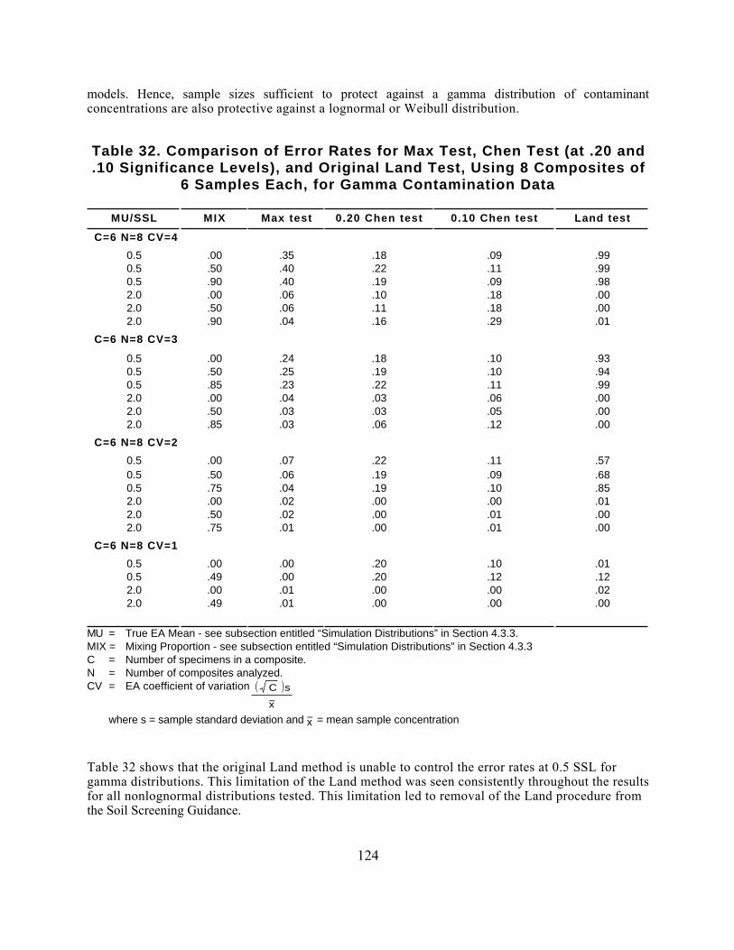
models. Hence, sample sizes sufficient to protect against a gamma distribution of contaminantconcentrations are also protective against a lognormal or Weibull distribution.
Table 32. Comparison of Error Rates for Max Test, Chen Test (at .20 and.10 Significance Levels), and Original Land Test, Using 8 Composites of
6 Samples Each, for Gamma Contamination Data
MU/SSL MIX Max test 0.20 Chen test 0.10 Chen test Land test
C=6 N=8 CV=4
0.50.50.52.02.02.0
.00
.50
.90
.00
.50
.90
.35
.40
.40
.06
.06
.04
.18
.22
.19
.10
.11
.16
.09
.11
.09
.18
.18
.29
.99
.99
.98
.00
.00
.01
C=6 N=8 CV=3
0.50.50.52.02.02.0
.00
.50
.85
.00
.50
.85
.24
.25
.23
.04
.03
.03
.18
.19
.22
.03
.03
.06
.10
.10
.11
.06
.05
.12
.93
.94
.99
.00
.00
.00
C=6 N=8 CV=2
0.50.50.52.02.02.0
.00
.50
.75
.00
.50
.75
.07
.06
.04
.02
.02
.01
.22
.19
.19
.00
.00
.00
.11
.09
.10
.00
.01
.01
.57
.68
.85
.01
.00
.00
C=6 N=8 CV=1
0.50.52.02.0
.00
.49
.00
.49
.00
.00
.01
.01
.20
.20
.00
.00
.10
.12
.00
.00
.01
.12
.02
.00
MU = True EA Mean - see subsection entitled “Simulation Distributions” in Section 4.3.3.MIX = Mixing Proportion - see subsection entitled “Simulation Distributions” in Section 4.3.3C = Number of specimens in a composite.N = Number of composites analyzed.CV = EA coefficient of variation C s
− x
where s = sample standard deviation and − x = mean sample concentration
Table 32 shows that the original Land method is unable to control the error rates at 0.5 SSL forgamma distributions. This limitation of the Land method was seen consistently throughout the resultsfor all nonlognormal distributions tested. This limitation led to removal of the Land procedure fromthe Soil Screening Guidance.
124
Earlier simulation results for gamma and Weibull distributions did not censor results below the QL andused pure unmixed distributions. In these cases, as the sample size N increased, with all other factorsfixed, the Land error rates at 0.5 SSL increased toward 1. Normally, the expectation is that as thesample size increases, information increases, and error rates decrease.
When using data from a Weibull or gamma distribution, the Land confidence interval endpointsconverge to a value that does not equal the true site mean, µx , and results in an increase in errorrates. This phenomenon is easily demonstrated, as follows. Let X denote the concentration randomvariable, let Y = ln(X) denote its logarithm. Let µy and σy denote the mean and standard deviation oflogarithms of the soil concentrations. Then, as the sample size increases, the Land confidenceinterval endpoints (UL and LL) converge to
UL = LL = exp ( µ y + σ 2
y
2 ) . (67)
If X is lognormally distributed, this expression is the mean of X. If X has a Weibull or gammadistribution, this expression is not the mean of X. This inconsistency accounts for the increase inerror rates with sample size.
Table 32 also shows the fundamental difference between the Max test and the Chen test. For theMax test, the probability of error in deciding to walk away when the EA mean is 2.0 SSL is fairlystable, ranging from 0.01 to 0.06 across the different values of the CV. On the other hand, theseerror rates vary more across the CV values for the Chen test (e.g., from 0.00 to 0.29 for Chen test atthe 0.10 significance level). This occurs because the Chen test is designed to control the other typeof error rate (at 0.5 SSL). The Max test is presented in the 1995 Soil Screening Guidance (U.S. EPA,1995c) because of its simplicity and the stability of its control over the error rate at 2 SSL.
Table 33 shows error rate estimates for four to nine composite samples that each consist of four, six,or eight specimens for EAs with CVs of 2, 2.5, 3, or 3.5, and assuming a gamma distribution. Table33 should be adequate for most SSL planning purposes. However, more complete simulation resultsare reported in Appendix I.
Planning for CVs at least as large as 2 is recommended because it is known that CVs greater than 2occur in practice (e.g., for two of seven EAs in the Piazza Road simulations reported in Section4.3.6). One conclusion that can be drawn from Table 33 is that composite sample sizes of four areoften inadequate. Further support for this conclusion is reported in the Piazza Road simulationsdiscussed in Section 4.3.6.
Conclusions. The primary conclusions from the simulations are:
• For distributions other than lognormal, the Land procedure is prone to decide toinvestigate further at 0.5 SSL, when the correct decision is to walk away. It istherefore unsuitable for surface soil screening.
• Both the Max test and the Chen test perform acceptably under a variety ofdistributional assumptions and are potentially suitable for surface soil screening.
125

Table 33. Error Rates of Max Test and Chen Test at .2 (C20) and .1 (C10)Significance Level for CV = 2, 2.5, 3, 3.5
CV = 2.0 CV = 2.5 CV = 3.0 CV = 3.5
N MU/SSL Max C20 C10 Max C20 C10 Max C20 C10 Max C20 C10
C = 4445566778899
0.52.00.52.00.52.00.52.00.52.00.52.0
.09
.13
.11
.10
.11
.06
.12
.04
.16
.02
.16
.01
.20
.08
.21
.05
.21
.03
.20
.03
.19
.02
.21
.01
.11
.16
.10
.11
.12
.08
.10
.05
.09
.03
.11
.02
.14
.19
.15
.10
.21
.08
.25
.05
.25
.04
.28
.03
.18
.17
.18
.09
.20
.08
.22
.04
.20
.03
.20
.03
.09
.28
.09
.18
.10
.14
.11
.09
.09
.07
.09
.06
.19
.20
.26
.17
.28
.11
.31
.08
.36
.05
.36
.04
.18
.21
.20
.19
.21
.13
.20
.11
.20
.08
.18
.07
.08
.33
.08
.30
.11
.23
.09
.18
.10
.14
.09
.13
.24
.26
.26
.18
.31
.11
.36
.08
.42
.07
.44
.07
.20
.29
.20
.23
.19
.18
.18
.14
.20
.13
.22
.12
.10
.42
.09
.36
.09
.28
.10
.23
.09
.21
.12
.20
C = 6445566778899
0.52.00.52.00.52.00.52.00.52.00.52.0
.03
.14
.04
.09
.06
.04
.06
.02
.06
.02
.06
.01
.20
.03
.20
.02
.20
.01
.20
.00
.19
.00
.20
.00
.12
.08
.10
.05
.11
.02
.09
.01
.09
.01
.10
.01
.08
.16
.11
.09
.14
.06
.12
.05
.15
.02
.18
.02
.21
.08
.17
.04
.21
.03
.19
.02
.20
.01
.22
.01
.12
.17
.09
.10
.10
.07
.10
.04
.10
.03
.11
.02
.15
.17
.17
.13
.19
.09
.23
.06
.25
.03
.28
.03
.20
.14
.20
.10
.20
.07
.22
.06
.19
.03
.20
.02
.10
.24
.10
.18
.10
.14
.10
.10
.10
.05
.11
.04
.16
.20
.22
.15
.25
.09
.29
.08
.30
.04
.34
.03
.17
.19
.20
.13
.20
.10
.21
.09
.19
.06
.19
.05
.08
.33
.10
.24
.10
.19
.10
.14
.10
.11
.09
.09
C = 8
445566778899
0.52.00.52.00.52.00.52.00.52.00.52.0
.02
.12
.03
.07
.02
.04
.03
.03
.04
.02
.04
.01
.21
.02
.22
.01
.18
.00
.20
.00
.20
.00
.21
.00
.13
.05
.11
.02
.09
.01
.11
.00
.10
.00
.11
.00
.06
.15
.05
.09
.08
.06
.09
.04
.11
.02
.11
.02
.19
.04
.20
.02
.21
.01
.20
.01
.21
.01
.21
.00
.10
.09
.11
.06
.11
.02
.11
.01
.11
.01
.10
.01
.10
.17
.11
.09
.13
.07
.18
.04
.17
.04
.20
.01
.21
.09
.20
.04
.19
.04
.21
.02
.21
.01
.19
.00
.10
.17
.10
.10
.10
.07
.11
.04
.10
.03
.10
.01
.14
.19
.17
.12
.20
.08
.22
.05
.26
.03
.30
.02
.18
.14
.19
.08
.20
.07
.20
.05
.19
.03
.23
.02
.08
.25
.09
.17
.10
.13
.11
.09
.10
.06
.12
.04
MU = True EA Mean - see subsection entitled “Simulation Distributions” in Section 4.3.3.MIX= Mixing Proportion - see subsection entitled “Simulation Distributions” in Section 4.3.3 C = Number of specimens in a composite.N = Number of composites analyzed.CV = EA coefficient of variation C s
− x
where s = sample standard deviation and − x = mean sample concentration
126

4.3.4 Treatment of Observations Below the Limit of Quantitation. Testprocedures that are based on estimating a mean contaminant level for an EA, such as the Land andChen procedures, make use of each measured concentration value. For this reason, the use of allreported concentration measurements in such calculations should be considered regardless of theirmagnitude—that is, even if the measured levels fall below a quantitation level. One argument for thisapproach is that the QL is itself an estimate. Another is that some value will have to be substitutedfor any censored data point (i.e., a point reported as <QL), and the actual measured value is at leastas accurate as a substituted value.
The peer review of the Draft Soil Screening Guidance raised the following issue:
If such censored values do occur in a data set, what values should be used?
There is a substantial amount of literature on this subject and a variety of sophisticated approaches.In the context of SSLs, however, a simple approach is recommended. Consistent with generalSuperfund guidance, each observation reported as "<QL" shall be replaced with 0.5 QL forcomputation of the sample mean.
The evidence suggests that the ingestion SSL generally will be 2 orders of magnitude or more greaterthan the QL for most contaminants. In these cases, the results of soil screening will be insensitive toalternative procedures that could be used to substitute values for observations reported as "<QL."When the SSL is not much greater than the QL (e.g., SSL < 50 QL), the outcome of the soilscreening could be affected by the procedure used to substitute for "<QL" values.
The most conservative approach would be to substitute the concentration represented by the QLitself for all observations reported as "<QL." In the context of the SSLs, however, the simpleapproach of using 0.5 QL is suggested. This will be sufficiently conservative given the conservativefactors underlying the SSLs.
4.3.5 Multiple Hypothesis Testing Considerations. The Soil Screening Guidanceaddresses the following hypothesis testing problem for each EA:
H0: mean concentration of a given chemical ≥ 2 SSL versus
H1: mean concentration of a given chemical < 2 SSL.
The default value for the probability of a Type I error is α = 0.05, while the default value for thepower of the test at 0.5 SSL is 1-ß = 0.80. The test is applied separately for each chemical, so thatthese probabilities apply for each individual chemical. Thus, there is an 80 percent probability ofwalking away from an EA (i.e., rejecting H0) when only one chemical is being tested and its truemean level is 0.5 SSL and a 5 percent probability of walking away if its true mean level is 2 SSL.
However, the Soil Screening Guidance does not explicitly address the following issues:
What is the composite probability of walking away from an EA if there aremultiple contaminants?
andIf such probabilities are unacceptable, how should one compensate when testingfor multiple contaminants within a single EA?
127

The answer to the first question cannot be determined, in general, since the concentrations of thevarious contaminants will often be dependent on one another (e.g., this would be expected if theyoriginated from the same source of contamination). The joint probability of walking away can bedetermined, however, if one makes the simplifying assumption that the contaminant concentrationsfor the different chemicals are independent (uncorrelated). In that case, the probability of walkingaway is simply the product of the individual rejection probabilities.
For two chemicals (Chemical A and Chemical B, say), this is:
Prwalking away from EA = Prreject H0 for Chemical A H Prreject H0 for Chemical B.
While these joint probabilities must be regarded as approximate, they nevertheless serve to illustratethe effect on the error rates when dealing with multiple contaminants.
Assume (for illustrative purposes only) that the probabilities for rejecting the null hypothesis(walking away from the EA) for each single chemical appear as follows:
True concentration Probability of rejecting H0
0.2 SSL 0.950.5 SSL 0.80 (default 1-ß)0.7 SSL 0.601.0 SSL 0.501.5 SSL 0.202.0 SSL 0.05 (default α)
Let C(A) denote the concentration of Chemical A divided by the SSL, and let P(A) denote thecorresponding probability of rejecting H0. Define C(B) and P(B) similarly for Chemical B. Assumingindependence, the joint probabilities of rejecting the null hypothesis (walking away) are as shown inTable 34.
Table 34. Probability of "Walking Away" from an EA When ComparingTwo Chemicals to SSLs
Chemical A Chemical B
C(A) P(A)C(B) = 0.2P(B) =.95
C(B) = 0.5P(B) = .80
C(B) = 0.7P(B) = .60
C(B) = 1.0P(B) = .50
C(B) = 1.5P(B) = .20
C(B) = 2.0P(B) = .05
0.2 0.95 0.90 0.76 0.57 0.48 0.19 0.05
0.5 0.80 0.76 0.64 0.48 0.40 0.16 0.04
0.7 0.60 0.57 0.48 0.36 0.30 0.12 0.03
1.0 0.50 0.48 0.40 0.30 0.25 0.10 0.03
1.5 0.20 0.19 0.16 0.12 0.10 0.04 0.01
2.0 0.05 0.05 0.04 0.03 0.03 0.01 <0.01
128

These probabilities demonstrate that the test procedure will tend to be very conservative if multiplechemicals are involved—that is, all of the chemical concentrations must be quite low relative totheir SSL in order to have a high probability of walking away from the EA. On the other hand, therewill be a high probability that further investigation will be called for if the mean concentration foreven a single chemical is twice the SSL.
A potential problem occurs when there are several chemicals under consideration and when all ormost of them have levels slightly below the SSL (e.g., near 0.5 SSL). For instance, if each of sixindependent chemicals had levels at 0.5 SSL, the probability of rejecting the null hypothesis would be80 percent for each such chemical, but the probability of walking away from the EA would be only(0.80)6 = 0.26.
If the same samples are being analyzed for multiple chemicals, then the original choice for thenumber of such samples ideally should have been based on the worst case (i.e., the chemical expectedto have the largest variability). In this case, the probability of correctly rejecting the null hypothesisat 0.5 SSL for the chemicals with less variability will be higher. The overall probability of walkingaway will be greater than shown above if all or some of the chemicals have less variability thanassumed as the basis for determining sample sizes. Here, the sample size will be large enough for theprobability of rejecting the null hypothesis at 0.5 SSL to be greater than 0.80 for these chemicals.
The probability values assumed above for deciding that no further investigation is necessary forindividual chemicals, which are the basis for these conclusions, are equally applicable for the Land,Chen, and Max tests. They simply represent six hypothetical points of the power curves for thesetests (from 0.2 SSL to 2.0 SSL). Therefore, the conclusions are equally applicable for each of thehypothesis testing procedures that have been considered in the current guidance for screening surfacesoils.
If the surface soil concentrations are positively correlated, as expected when dealing with multiplechemicals, then it is likely that either all the chemicals of concern have relatively highconcentrations or they all have relatively low concentrations. In this case, the probability of makingthe correct decision for an EA would be greater than that suggested by the above calculations thatassume independence of the various chemicals.
However, the potential problem of several chemicals having concentrations near 0.5 SSL is notprecluded by assuming positive correlations. In fact, it suggests that if the EA average for onechemical is near 0.5 SSL, then the average for others is also likely to be near 0.5 SSL, which isexactly the situation where the probability of not walking away from the EA can become largebecause there is a high probability that H0 will be rejected for at least one of these chemicals.
An alternative would be to use multiple hypothesis testing procedures to control the overall errorrate for the set of chemicals (i.e., the set of hypothesis tests) rather than the separate error rates forthe individual chemicals. Guidance for performing multiple hypothesis tests is beyond the scope ofthe current document. Obtain the advice of a statistician familiar with multiple hypothesis testingprocedures if the overall error rates for multiple chemicals is of concern for a particular site. Theclassical statistical guidance regarding this subject is Simultaneous Statistical Inference (Miller, 1991).
4.3.6 Investigation of Compositing Within EA Sectors. If one decides that anEA needs further investigation, then it is natural to inquire which portion(s) of the EA exceed thescreening level. This is a different question than simply asking whether or not the EA average soilconcentration exceeds the SSL. Conceivably, this question may require additional sampling, chemical
129

analysis, and statistical analysis. A natural question is whether this additional effort can be avoided byforming composites within sectors (subareas) of the EA. The sector with the highest estimatedconcentration would then be a natural place to begin a detailed investigation.
The simulations to investigate the performance of rules to decide whether further investigation isrequired, reported in Section 4.3.3, make specific assumptions about the sampling design. It isassumed that N composite samples are chemically analyzed, each consisting of C specimens selectedto be statistically representative of the entire EA. The key point, in addition to random sampling, isthat composites must be formed across sectors rather than within sectors. This assumption isnecessary to achieve composite samples that are representative of the EA mean (i.e., have the EAmean as their expected value).
If compositing is limited to sectors, such as quadrants, then each composite represents its sector,rather than the entire EA. The simulations reported in Section 4.3.3, and sample sizes based onthem, do not apply to this type of compositing. This does not necessarily preclude compositingwithin sectors for both purposes, i.e., to test the hypothesis about the EA mean and also to indicatethe most contaminated sector. However, little is known about the statistical properties of thisapproach when applying the Max test, which would depend on specifics of the actual spatialdistribution of contaminants for a given EA. Because of the lack of extensive spatial data sets forcontaminated soil, there is limited basis for determining what sample sizes would be adequate forachieving desired DQOs for various sites. However, one spatial data set was available and used toinvestigate the performance of compositing within sectors at one site.
Piazza Road Simulations. Data from the Piazza Road NPL site were used to investigate theproperties of tests of the EA mean based on compositing within sectors, as compared to compositingbetween sectors. The investigation of a single site cannot be used to validate a given procedure, but itmay indicate whether further investigation of the procedure is worthwhile.
Seven nonoverlapping 0.4-acre EAs were defined within the Piazza Road site. Each EA is an 8-by-12grid composed of 14'x14' squares. The data consist of a single dioxin measurement of a compositesample from each small square. These measurements are regarded as true values for the simulationsreported in this section. Measurement error was incorporated in the same fashion as for thesimulations reported in Section 4.3.3.
Each of the seven EAs was subdivided into four 4-by-6 sectors, six 4-by-4 sectors, eight 4-by-3sectors, twelve 2-by-4 sectors, and sixteen 2-by-3 sectors. Results are presented here for the cases offour, six, and eight sectors because composites of more than eight specimens are expected to be usedrarely, if at all.
Table 35 presents the "true" mean and CV for each EA, computed from all 96 measurements withinthe 0.4-acre EA. The CVs range from 1.0 to 2.2. Note that two of the seven CVs equal or exceed 2at this site. This supports EPA's belief that at many sites it is prudent, when planning sample sizerequirements for screening, to assume a CV of at least 2.5 and to consider the possibility of CVs aslarge as 3 or 3.5.
As data on variability within EAs for different sites and contaminant conditions accrue over time, itwill be possible to base the choice of procedures on a larger, more comprehensive database, ratherthan just a single site.
Appendix J contains results of simulations from the seven Piazza Road EAs. Sampling with
130

replacement from each sector was used, because this was felt to be more consistent with the plannedcompositing. To estimate the error rates at 0.5 SSL and 2 SSL for each EA, the SSL was defined sothat the site mean first was regarded as 0.5 SSL and then was regarded as 2 SSL.
Notation for Results from Piazza Road Simulations. The following notation is usedin Appendix J. The design variable (DES) indicates whether compositing was within sector (DES=W)or across sectors (DES=X). As in Section 4.3.3, C denotes the number of specimens per composite,and N denotes the number of composite samples chemically analyzed. Results in Appendix J are forthe Chen test at the 10 percent significance level and for the Max test. The true mean and CV areshown in the header for each EA.
Table 35. Means and CVs for Dioxin Concentrations for 7 Piazza RoadExposure Areas
EA Mean of EA CV of EA N
1 2.1 1.0 96
2 2.4 1.6 96
3 5.1 1.1 96
4 4.0 1.2 96
5 9.3 2.0 96
6 15.8 2.2 96
7 2.8 1.4 96
Results and Conclusions from Piazza Road Simulations. Although the resultsfrom a single site cannot be assumed to apply to all sites, the following observations can be madebased on the Piazza Road simulations reported in Appendix J.
• The error rate at 0.5 SSL for the Chen test, using compositing across sectors(DES=X), is generally close to the nominal rate of 0.10. For compositing withinsectors (DES=W), the error rate for Chen at 0.5 SSL is generally much lower than thenominal rate.
• Except for plans involving only four analyses (N = 4), the error rate at 2 SSL isalways below 0.05 for the Chen test. For the Max test, the error rate at 2 SSLfluctuated between 0 and 16 percent. The error rate at 2 SSL is smaller for the Chentest at the 10 percent significance level than for the Max test in virtually all cases.The only two exceptions to this are for compositing within sector (DES=W) in EANo. 6.
• This observation provides further support for the conclusion drawn from thesimulations reported in Section 4.3.3: plans involving only four analyses can result inhigh error rates in determining the mean contaminant concentration of an EA withthe Max test. In most cases the error rates of concern to EPA (at 2 SSL) are 0.10 orlarger.
131

• In general, error rates estimated from Piazza Road simulations for compositing acrosssectors are at least as small as would be predicted on the basis of the simulation resultsreported in Section 4.3.3.
• The simulation results show that compositing within sectors using the Max test maybe an option for site managers who want to know whether one sector of an EA ismore contaminated than the other. However, use of the Max test when compositingwithin sectors may lead the site manager to draw conclusions about the meancontaminant concentration in that sector only, not across the entire EA.
132

Part 5: CHEMICAL-SPECIFIC PARAMETERS
Chemical-specific parameters required for calculating soil screening levels include the organic carbonnormalized soil-water partition coefficient for organic compounds (Koc), the soil-water partitioncoefficient for inorganic constituents (Kd), water solubility (S), Henry's law constant (HLC, HN), airdiffusivity (Di,a), and water diffusivity (Di,w). In addition, the octanol-water partition coefficient(Kow) is needed to calculate Koc values. This part of the background document describes thecollection and compilation of these parameters for the SSL chemicals.
With the exception of values for air diffusivity (Di,a), water diffusivity (Di,w), and certain Koc values,all of the values used in the development of SSLs can be found in the Superfund Chemical DataMatrix (SCDM). SCDM is a computer code that includes more than 25 datafiles containing specificchemical parameters used to calculate factor and benchmark values for the Hazard Ranking System(HRS). Because SCDM datafiles are regularly updated, the user should consult the most recent versionof SCDM to ensure that the values are up to date.
5.1 Solubility, Henry's Law Constant, and Kow
Chemical-specific values for solubility, Henry's law constant (HLC), and Kow were obtained fromSCDM. In the selection of the value for SCDM, measured or analytical values are favored overcalculated values. However, in the event that a measured value is not available, calculated values areused. Table 36 presents the solubility, Henry's law constant, and Kow values taken from SCDM andused to calculate SSLs.
Henry's law constant values were available for all but two of the constituents of interest. Henry's lawconstants could not be obtained from the SCDM datafiles for either carbazole or mercury. As aconsequence, this parameter was calculated according to the following equation:
HLC = (VP)(M)/(S) (68)where
HLC = Henry's law constant (atm-m3/mol)VP = vapor pressure (atm)M = molecular weight (g/mol)S = solubility (mg/L or g/m3).
The SSL equations require the dimensionless form of Henry's law constant, or H', which is calculatedfrom HLC (atm-m3/mol) by multiplying by 41 (U.S. EPA, 1991b). The values taken from SCDM forHLC and the calculated dimensionless values for H' are both presented in Table 36.
5.2 Air (Di ,a) and Water (D i,w) Diffusivities
Few published diffusivities were available for the subject chemicals for air (Di,a) and water (Di,w).Water and air diffusivities were obtained from the CHEMDAT8 model chemical properties database(DATATWO.WK1). For chemicals not in CHEMDAT8, diffusivities were estimated using the
133

WATER8 model correlations for air and water diffusivities. Both CHEMDAT8 and WATER8 can beobtained from EPA's SCRAM bulletin board system, as described in Section 3.1.2. Table 37 presentsthe values used to calculate SSLs.
Table 36. Chemical-Specific Properties Used in SSL Calculations
CAS No. CompoundS
(mg/L)HLC
(atm-m3/mol)HN
(dimensionless) log Kow
83-32-9 Acenaphthene 4.24E+00 1.55E-04 6.36E-03 3.9267-64-1 Acetone 1.00E+06 3.88E-05 1.59E-03 -0.24
309-00-2 Aldrin 1.80E-01 1.70E-04 6.97E-03 6.50120-12-7 Anthracene 4.34E-02 6.50E-05 2.67E-03 4.55
56-55-3 Benz(a)anthracene 9.40E-03 3.35E-06 1.37E-04 5.7071-43-2 Benzene 1.75E+03 5.55E-03 2.28E-01 2.13
205-99-2 Benzo(b)fluoranthene 1.50E-03 1.11E-04 4.55E-03 6.20207-08-9 Benzo(k)fluoranthene 8.00E-04 8.29E-07 3.40E-05 6.20
65-85-0 Benzoic acid 3.50E+03 1.54E-06 6.31E-05 1.86
50-32-8 Benzo(a)pyrene 1.62E-03 1.13E-06 4.63E-05 6.11111-44-4 Bis(2-chloroethyl)ether 1.72E+04 1.80E-05 7.38E-04 1.21117-81-7 Bis(2-ethylhexyl)phthalate 3.40E-01 1.02E-07 4.18E-06 7.30
75-27-4 Bromodichloromethane 6.74E+03 1.60E-03 6.56E-02 2.10
75-25-2 Bromoform 3.10E+03 5.35E-04 2.19E-02 2.3571-36-3 Butanol 7.40E+04 8.81E-06 3.61E-04 0.8585-68-7 Butyl benzyl phthalate 2.69E+00 1.26E-06 5.17E-05 4.8486-74-8 Carbazole 7.48E+00 1.53E-08 a 6.26E-07 3.5975-15-0 Carbon disulfide 1.19E+03 3.03E-02 1.24E+00 2.00
56-23-5 Carbon tetrachloride 7.93E+02 3.04E-02 1.25E+00 2.7357-74-9 Chlordane 5.60E-02 4.86E-05 1.99E-03 6.32
106-47-8 p-Chloroaniline 5.30E+03 3.31E-07 1.36E-05 1.85108-90-7 Chlorobenzene 4.72E+02 3.70E-03 1.52E-01 2.86
124-48-1 Chlorodibromomethane 2.60E+03 7.83E-04 3.21E-02 2.1767-66-3 Chloroform 7.92E+03 3.67E-03 1.50E-01 1.9295-57-8 2-Chlorophenol 2.20E+04 3.91E-04 1.60E-02 2.15
218-01-9 Chrysene 1.60E-03 9.46E-05 3.88E-03 5.7072-54-8 DDD 9.00E-02 4.00E-06 1.64E-04 6.10
72-55-9 DDE 1.20E-01 2.10E-05 8.61E-04 6.7650-29-3 DDT 2.50E-02 8.10E-06 3.32E-04 6.5353-70-3 Dibenz(a,h)anthracene 2.49E-03 1.47E-08 6.03E-07 6.6984-74-2 Di-n-butyl phthalate 1.12E+01 9.38E-10 3.85E-08 4.6195-50-1 1,2-Dichlorobenzene 1.56E+02 1.90E-03 7.79E-02 3.43
106-46-7 1,4-Dichlorobenzene 7.38E+01 2.43E-03 9.96E-02 3.4291-94-1 3,3-Dichlorobenzidine 3.11E+00 4.00E-09 1.64E-07 3.5175-34-3 1,1-Dichloroethane 5.06E+03 5.62E-03 2.30E-01 1.79
134

Table 36 (continued)
CAS No. CompoundS
(mg/L)HLC
(atm-m3/mol)HN
(dimensionless) log Kow
107-06-2 1,2-Dichloroethane 8.52E+03 9.79E-04 4.01E-02 1.4775-35-4 1,1-Dichloroethylene 2.25E+03 2.61E-02 1.07E+00 2.13
156-59-2 cis-1,2-Dichloroethylene 3.50E+03 4.08E-03 1.67E-01 1.86156-60-5 trans-1,2-Dichloroethylene 6.30E+03 9.38E-03 3.85E-01 2.07
120-83-2 2,4-Dichlorophenol 4.50E+03 3.16E-06 1.30E-04 3.0878-87-5 1,2-Dichloropropane 2.80E+03 2.80E-03 1.15E-01 1.97
542-75-6 1,3-Dichloropropene 2.80E+03 1.77E-02 7.26E-01 2.0060-57-1 Dieldrin 1.95E-01 1.51E-05 6.19E-04 5.3784-66-2 Diethylphthalate 1.08E+03 4.50E-07 1.85E-05 2.50
105-67-9 2,4-Dimethylphenol 7.87E+03 2.00E-06 8.20E-05 2.3651-28-5 2,4-Dinitrophenol 2.79E+03 4.43E-07 1.82E-05 1.55
121-14-2 2,4-Dinitrotoluene 2.70E+02 9.26E-08 3.80E-06 2.01606-20-2 2,6-Dinitrotoluene 1.82E+02 7.47E-07 3.06E-05 1.87
117-84-0 Di-n-octyl phthalate 2.00E-02 6.68E-05 2.74E-03 8.06115-29-7 Endosulfan 5.10E-01 1.12E-05 4.59E-04 4.10
72-20-8 Endrin 2.50E-01 7.52E-06 3.08E-04 5.06100-41-4 Ethylbenzene 1.69E+02 7.88E-03 3.23E-01 3.14206-44-0 Fluoranthene 2.06E-01 1.61E-05 6.60E-04 5.12
86-73-7 Fluorene 1.98E+00 6.36E-05 2.61E-03 4.2176-44-8 Heptachlor 1.80E-01 1.09E-03 4.47E-02 6.26
1024-57-3 Heptachlor epoxide 2.00E-01 9.50E-06 3.90E-04 5.00118-74-1 Hexachlorobenzene 6.20E+00 1.32E-03 5.41E-02 5.89
87-68-3 Hexachloro-1,3-butadiene 3.23E+00 8.15E-03 3.34E-01 4.81319-84-6 α-HCH (α-BHC) 2.00E+00 1.06E-05 4.35E-04 3.80319-85-7 β-HCH (β-BHC) 2.40E-01 7.43E-07 3.05E-05 3.81
58-89-9 γ -HCH (Lindane) 6.80E+00 1.40E-05 5.74E-04 3.7377-47-4 Hexachlorocyclopentadiene 1.80E+00 2.70E-02 1.11E+00 5.39
67-72-1 Hexachloroethane 5.00E+01 3.89E-03 1.59E-01 4.00193-39-5 Indeno(1,2,3-cd)pyrene 2.20E-05 1.60E-06 6.56E-05 6.65
78-59-1 Isophorone 1.20E+04 6.64E-06 2.72E-04 1.707439-97-6 Mercury --- 1.14E-02 b 4.67E-01 ---
72-43-5 Methoxychlor 4.50E-02 1.58E-05 6.48E-04 5.08
74-83-9 Methyl bromide 1.52E+04 6.24E-03 2.56E-01 1.1975-09-2 Methylene chloride 1.30E+04 2.19E-03 8.98E-02 1.2595-48-7 2-Methylphenol 2.60E+04 1.20E-06 4.92E-05 1.9991-20-3 Naphthalene 3.10E+01 4.83E-04 1.98E-02 3.36
98-95-3 Nitrobenzene 2.09E+03 2.40E-05 9.84E-04 1.8486-30-6 N-Nitrosodiphenylamine 3.51E+01 5.00E-06 2.05E-04 3.16
621-64-7 N-Nitrosodi-n-propylamine 9.89E+03 2.25E-06 9.23E-05 1.40
135

Table 36 (continued)
CAS No. CompoundS
(mg/L)HLC
(atm-m3/mol)HN
(dimensionless) log Kow
87-86-5 Pentachlorophenol 1.95E+03 2.44E-08 1.00E-06 5.09108-95-2 Phenol 8.28E+04 3.97E-07 1.63E-05 1.48129-00-0 Pyrene 1.35E-01 1.10E-05 4.51E-04 5.11100-42-5 Styrene 3.10E+02 2.75E-03 1.13E-01 2.94
79-34-5 1,1,2,2-Tetrachloroethane 2.97E+03 3.45E-04 1.41E-02 2.39127-18-4 Tetrachloroethylene 2.00E+02 1.84E-02 7.54E-01 2.67108-88-3 Toluene 5.26E+02 6.64E-03 2.72E-01 2.75
8001-35-2 Toxaphene 7.40E-01 6.00E-06 2.46E-04 5.50120-82-1 1,2,4-Trichlorobenzene 3.00E+02 1.42E-03 5.82E-02 4.01
71-55-6 1,1,1-Trichloroethane 1.33E+03 1.72E-02 7.05E-01 2.4879-00-5 1,1,2-Trichloroethane 4.42E+03 9.13E-04 3.74E-02 2.0579-01-6 Trichloroethylene 1.10E+03 1.03E-02 4.22E-01 2.7195-95-4 2,4,5-Trichlorophenol 1.20E+03 4.33E-06 1.78E-04 3.90
88-06-2 2,4,6-Trichlorophenol 8.00E+02 7.79E-06 3.19E-04 3.70108-05-4 Vinyl acetate 2.00E+04 5.11E-04 2.10E-02 0.73
75-01-4 Vinyl chloride 2.76E+03 2.70E-02 1.11E+00 1.50108-38-3 m-Xylene 1.61E+02 7.34E-03 3.01E-01 3.20
95-47-6 o-Xylene 1.78E+02 5.19E-03 2.13E-01 3.13
106-42-3 p-Xylene 1.85E+02 7.66E-03 3.14E-01 3.17CAS = Chemical Abstracts Service.S = Solubility in water (20-25 °C).HLC = Henry's law constant.HN = Dimensionless Henry's law constant (HLC [atm-m3/mol] * 41) (25 °C).Kow = Octanol/water partition coefficient.a HLC was calculated using the equation: HLC = vapor pressure * molecular wt. / solubility. Vapor pressure is 6.83E-10
atm and molecular weight is 167.21 g/mol for carbazole.b Value from WATER8 model database.
136

Table 37. Air Diffusivity (Di ,a) and Water Diffusivity (Di,w) Values for SSL Chemicals (25 C)a
CAS No. Compound D i,a (cm2/s) D i,w (cm2/s)
83-32-9 Acenaphthene 4.21E-02 7.69E-06 67-64-1 Acetone 1.24E-01 1.14E-05
309-00-2 Aldrin 1.32E-02 4.86E-06 120-12-7 Anthracene 3.24E-02 7.74E-06
56-55-3 Benz(a)anthracene 5.10E-02 9.00E-06 71-43-2 Benzene 8.80E-02 9.80E-06
205-99-2 Benzo(b)fluoranthene 2.26E-02 5.56E-06 207-08-9 Benzo(k)fluoranthene 2.26E-02 5.56E-06
65-85-0 Benzoic acid 5.36E-02 7.97E-06
50-32-8 Benzo(a)pyrene 4.30E-02 9.00E-06 111-44-4 Bis(2-chloroethyl)ether 6.92E-02 7.53E-06 117-81-7 Bis(2-ethylhexyl)phthalate 3.51E-02 3.66E-06
75-27-4 Bromodichloromethane 2.98E-02 1.06E-05
75-25-2 Bromoform 1.49E-02 1.03E-05 71-36-3 Butanol 8.00E-02 9.30E-06 85-68-7 Butyl benzyl phthalate 1.74E-02 b 4.83E-06 b
86-74-8 Carbazole 3.90E-02 b 7.03E-06 b
75-15-0 Carbon disulfide 1.04E-01 1.00E-05
56-23-5 Carbon tetrachloride 7.80E-02 8.80E-06 57-74-9 Chlordane 1.18E-02 4.37E-06
106-47-8 p-Chloroaniline 4.83E-02 1.01E-05 108-90-7 Chlorobenzene 7.30E-02 8.70E-06
124-48-1 Chlorodibromomethane 1.96E-02 1.05E-05 67-66-3 Chloroform 1.04E-01 1.00E-05 95-57-8 2-Chlorophenol 5.01E-02 9.46E-06
218-01-9 Chrysene 2.48E-02 6.21E-06 72-54-8 DDD 1.69E-02 b 4.76E-06 b
72-55-9 DDE 1.44E-02 5.87E-06 50-29-3 DDT 1.37E-02 4.95E-06 53-70-3 Dibenz(a,h)anthracene 2.02E-02 b 5.18E-06 b
84-74-2 Di-n-butyl phthalate 4.38E-02 7.86E-06 95-50-1 1,2-Dichlorobenzene 6.90E-02 7.90E-06
106-46-7 1,4-Dichlorobenzene 6.90E-02 7.90E-06 91-94-1 3,3-Dichlorobenzidine 1.94E-02 6.74E-06 75-34-3 1,1-Dichloroethane 7.42E-02 1.05E-05
107-06-2 1,2-Dichloroethane 1.04E-01 9.90E-06
75-35-4 1,1-Dichloroethylene 9.00E-02 1.04E-05 156-59-2 cis-1,2-Dichloroethylene 7.36E-02 1.13E-05 156-60-5 trans-1,2-Dichloroethylene 7.07E-02 1.19E-05 120-83-2 2,4-Dichlorophenol 3.46E-02 8.77E-06
137

Table 37 (continued)
CAS No. Compound D i,a (cm2/s) D i,w (cm2/s)
78-87-5 1,2-Dichloropropane 7.82E-02 8.73E-06 542-75-6 1,3-Dichloropropene 6.26E-02 1.00E-05
60-57-1 Dieldrin 1.25E-02 4.74E-06 84-66-2 Diethylphthalate 2.56E-02 b 6.35E-06 b
105-67-9 2,4-Dimethylphenol 5.84E-02 8.69E-06 51-28-5 2,4-Dinitrophenol 2.73E-02 9.06E-06
121-14-2 2,4-Dinitrotoluene 2.03E-01 7.06E-06 606-20-2 2,6-Dinitrotoluene 3.27E-02 7.26E-06 117-84-0 Di-n-octyl phthalate 1.51E-02 3.58E-06
115-29-7 Endosulfan 1.15E-02 4.55E-06 72-20-8 Endrin 1.25E-02 4.74E-06
100-41-4 Ethylbenzene 7.50E-02 7.80E-06 206-44-0 Fluoranthene 3.02E-02 6.35E-06
86-73-7 Fluorene 3.63E-02 b 7.88E-06 b
76-44-8 Heptachlor 1.12E-02 5.69E-06 1024-57-3 Heptachlor epoxide 1.32E-02 b 4.23E-06 b
118-74-1 Hexachlorobenzene 5.42E-02 5.91E-06 87-68-3 Hexachloro-1,3-butadiene 5.61E-02 6.16E-06
319-84-6 α-HCH (α-BHC) 1.42E-02 7.34E-06 319-85-7 β-HCH (β-BHC) 1.42E-02 7.34E-06
58-89-9 γ -HCH (Lindane) 1.42E-02 7.34E-06 77-47-4 Hexachlorocyclopentadiene 1.61E-02 7.21E-06
67-72-1 Hexachloroethane 2.50E-03 6.80E-06 193-39-5 Indeno(1,2,3-cd)pyrene 1.90E-02 5.66E-06
78-59-1 Isophorone 6.23E-02 6.76E-06 7439-97-6 Mercury 3.07E-02 b 6.30E-06 b
72-43-5 Methoxychlor 1.56E-02 4.46E-06
74-83-9 Methyl bromide 7.28E-02 1.21E-05 75-09-2 Methylene chloride 1.01E-01 1.17E-05 95-48-7 2-Methylphenol 7.40E-02 8.30E-06 91-20-3 Naphthalene 5.90E-02 7.50E-06 98-95-3 Nitrobenzene 7.60E-02 8.60E-06
86-30-6 N-Nitrosodiphenylamine 3.12E-02 b 6.35E-06 b
621-64-7 N-Nitrosodi-n-propylamine 5.45E-02 b 8.17E-06 b
87-86-5 Pentachlorophenol 5.60E-02 6.10E-06 108-95-2 Phenol 8.20E-02 9.10E-06
129-00-0 Pyrene 2.72E-02 b 7.24E-06 b
100-42-5 Styrene 7.10E-02 8.00E-06 79-34-5 1,1,2,2-Tetrachloroethane 7.10E-02 7.90E-06
127-18-4 Tetrachloroethylene 7.20E-02 8.20E-06
138

Table 37 (continued)
CAS No. Compound D i,a (cm2/s) D i,w (cm2/s)
108-88-3 Toluene 8.70E-02 8.60E-06 8001-35-2 Toxaphene 1.16E-02 4.34E-06
120-82-1 1,2,4-Trichlorobenzene 3.00E-02 8.23E-06 71-55-6 1,1,1-Trichloroethane 7.80E-02 8.80E-06
79-00-5 1,1,2-Trichloroethane 7.80E-02 8.80E-06 79-01-6 Trichloroethylene 7.90E-02 9.10E-06 95-95-4 2,4,5-Trichlorophenol 2.91E-02 7.03E-06 88-06-2 2,4,6-Trichlorophenol 3.18E-02 6.25E-06
108-05-4 Vinyl acetate 8.50E-02 9.20E-06
75-01-4 Vinyl chloride 1.06E-01 1.23E-06 108-38-3 m-Xylene 7.00E-02 7.80E-06
95-47-6 o-Xylene 8.70E-02 1.00E-05 106-42-3 p-Xylene 7.69E-02 8.44E-06
CAS = Chemical Abstracts Service.a Value from CHEMDAT8 model database unless indicated otherwise.b Estimated using correlations in WATER8 model.
5.3 Soil Organic Carbon/Water Partition Coefficients (Koc)
Application of SSLs for the inhalation and migration to ground water pathways requires Koc valuesfor each organic chemical of concern. Koc values are also needed for site-specific exposure modelingefforts. An initial review of the literature uncovered significant variability in this parameter, withreported measured values for a compound sometimes varying over several orders of magnitude. Thisvariability can be attributed to several factors, including actual variability due to differences in soil orsediment properties, differences in experimental and analytical approaches used to measure thevalues, and experimental or measurement error. To resolve this difficulty, an extensive literaturereview was conducted to uncover all available measured values and to identify approaches andinformation that might be useful in developing valid Koc values.
The soil-water partitioning behavior of nonionizing and ionizing organic compounds differs becausethe partitioning of ionizing organics can be significantly influenced by soil pH. For this reason,different approaches were required to estimate Koc values for nonionizing and ionizing organiccompounds.
5.3.1 Koc for Nonionizing Organic Compounds. As noted earlier, there issignificant variability in reported Koc values and an extensive literature search was conducted tocollect all available measured Koc values for the nonionizing hydrophobic organic compounds ofinterest.
In the literature search, misquotation error was minimized by obtaining the original referenceswhenever possible. Values from compilations and secondary references were used only when theoriginal references could not be obtained. Redundancy of values was avoided, although in rare
139

instances it was not possible to determine if compilations included such values, especially when datawere reported as "selected" values.
In certain references, soil-water partition coefficients (e.g., Kd or Kp) were reported along with theorganic carbon content of the soil. In these cases, Koc was computed by dividing Kd by the fractionalsoil organic carbon content (foc, g/g). If the partition coefficient was normalized to soil organicmatter (i.e., Kom), it was converted to Koc as follows (Dragun, 1988):
Koc = 1.724 Kom (69)
where
1.724 = conversion factor from organic matter to organic carbon (fom = 1.724 foc )Kom = partition coefficient normalized to organic matter (L/kg)fom = fraction organic matter (g/g).
Once collected, Koc values were reviewed. It was not possible to systematically evaluate each sourcefor accuracy or consistency or to analyze sources of variability between references because of widevariations in soil and sediment properties, experimental and analytical methods, and the manner inwhich these were reported in each reference. This, and the limited number of Koc values for manycompounds, prevented any meaningful statistical analysis to eliminate outliers.
Collected values were qualitatively reviewed, however, and some values were excluded. Valuesmeasured for low-carbon-content sorbents (i.e., foc ≤ 0.001) are generally beyond the range of thelinear relationship between soil organic carbon and Kd and were rejected in most cases. Somereferences produced consistently high or low values and, as a result, were eliminated. Values were alsoeliminated if they fell outside the range of other measured values. The final values used are presentedin Appendix K along with their reference sources.
Summary statistics for the measured Koc values are presented in Table 38. The geometric mean ofthe Koc for each nonionizing organic compound is used as the the central tendency Koc value becauseit is a more suitable estimate of the central tendency of a distribution of environmental values withwide variability.
The data contained in Table 38 are summarized in Table 39 for each of the nonionizing organiccompounds for which measured Koc values were available. As shown, measured values are available foronly a subset of the SSL compounds. As a consequence, an alternative methodology was applied todetermine Koc values for the entire set of nonionizing hydrophobic organic compounds of interest.
It has long been noted that a strong linear relationship exists between Koc and Kow (octanol/waterpartition coefficient) (Lyman et al., 1982) and that this relationship can be used to predict Koc in theabsence of measured data. One such relationship was reported by Di Toro (1985). This relationshipwas selected for use in calculating Koc values for most semivolatile nonionizing organic compounds(Group 1 in Table 39) because it considers particle interaction and was shown to be in conformitywith observations for a large set of adsorption-desorption data (Di Toro, 1985). Di Toro's equation isas follows:
log Koc = 0.00028 + (0.983 H log Kow) (70)
140

For volatile organic compounds (VOCs), Equation 70 consistently overpredicted Koc values whencompared to measured data. For this reason, a separate regression equation was developed using logKow and measured log Koc values for VOCs, chlorinated benzenes, and certain chlorinated pesticides:
log Koc = 0.0784 + (0.7919 H log Kow) (71)
Equation 71 was developed from a linear regression calculated at the 95 percent confidence level.The correlation coefficient (r) was 0.99 with an r2 of 0.97. The compounds and data used to developthis equation are provided in Appendix K. Equation 71 was used to calculate Koc values for VOCs,chlorobenzenes, and certain chlorinated pesticides (i.e., Group 2 in Table 39). Log Koc valuescalculated using Equations 70 and 71 were rounded to two decimal places, and the resulting Koc valueswere rounded to two decimal places in scientific notation (i.e, as they appear in Table 39) prior tocalculating SSLs.
Table 38. Summary Statistics for Measured Koc Values: NonionizingOrganicsa
Koc (L/kg)
CompoundGeometric
Mean Average Minimum MaximumSample
Size
Acenaphthene 4,898 5,028 3,890 6,166 2Aldrin 48,685 48,686 48,394 48,978 2Anthracene 23,493 24,362 14,500 33,884 9Benz(a)anthracene 357,537 459,882 150,000 840,000 4Benzene 62 66 31 100 13Benzo(a)pyrene 968,774 1,166,733 478,947 2,130,000 3
Bis(2-chloroethyl)ether 76 76 76 76 1Bis(2-ethylhexyl)phthalate 111,123 114,337 87,420 141,254 2Bromoform 126 126 126 126 1Butyl benzyl phthalate 13,746 14,055 11,128 16,981 2Carbon tetrachloride 152 158 123 224 3Chlordane 51,310 51,798 44,711 58,884 2
Chlorobenzene 224 260 83 500 9Chloroform 53 57 28 81 5DDD 45,800 45,800 45,800 45,800 1DDE 86,405 86,405 86,405 86,405 1DDT 677,934 792,158 285,467 1,741,516 6Dibenz(a,h)anthracene 1,789,101 2,029,435 565,014 3,059,425 14
1,2-Dichlorobenzene (o) 379 390 267 529 91,4-Dichlorobenzene (p) 616 687 273 1,375 161,1-Dichloroethane 53 54 46 62 21,2-Dichloroethane 38 44 22 76 31,1-Dichloroethylene 65 65 65 65 1
141

Table 38 (continued)
Koc (L/kg)
CompoundGeometric
Mean Average Minimum MaximumSample
Size
trans-1,2-Dichloroethylene 38 38 38 38 11,2-Dichloropropane 47 47 47 47 11,3-Dichloropropene 27 27 24 32 3Dieldrin 25,546 25,604 23,308 27,399 3Diethylphthalate 82 84 69 98 2Di-n-butylphthalate 1,567 1,580 1,384 1,775 2
Endosulfan 2,040 2,040 2,040 2,040 1Endrin 10,811 11,422 7,724 15,885 4Ethylbenzene 204 207 165 255 5Fluoranthene 49,096 49,433 41,687 54,954 3Fluorene 7,707 8,906 3,989 16,218 6Heptachlor 9,528 10,070 6,810 13,330 2
Hexachlorobenzene 80,000 80,000 80,000 80,000 1α-HCH (α-BHC) 1,762 1,835 1,022 2,891 12β-HCH (β-BHC) 2,139 2,241 1,156 3,563 14γ -HCH (Lindane) 1,352 1,477 731 3,249 65Methoxychlor 80,000 80,000 80,000 80,000 1Methyl bromide 9 9 9 9 1
Methyl chloride 6 6 6 6 1Methylene chloride 10 10 10 10 1Naphthalene 1,191 1,231 830 1,950 20Nitrobenzene 119 141 31 270 10Pentachlorobenzene 32,148 36,114 11,381 55,176 5Pyrene 67,992 70,808 43,807 133,590 27Styrene 912 912 912 912 1
1,1,2,2-Tetrachloroethane 79 79 79 79 1Tetrachloroethylene 265 272 177 373 15Toluene 140 145 94 247 12Toxaphene 95,816 95,816 95,816 95,816 11,2,4-Trichlorobenzene 1,659 1,783 864 3,125 171,1,1-Trichloroethane 135 139 106 179 5
1,1,2-Trichloroethane 75 77 60 108 4Trichloroethylene 94 97 57 150 21o-Xylene 241 241 222 258 4m-Xylene 196 204 158 289 3p-Xylene 311 313 260 347 3a See Appendix K for sources of measured values.
142

Table 39. Comparison of Measured and Calculated Koc Values
CAS No. CompoundChemicalGroup a
LogKow
Log Koc(L/kg)
CalculatedKoc
(L/kg)
MeasuredKoc
(L/kg)
83-32-9 Acenaphthene 1 3.92 3.85 7.08E+03 4.90E+0367-64-1 Acetone 1 -0.24 -0.24 5.75E-01 ---
309-00-2 Aldrin 1 6.50 6.39 2.45E+06 4.87E+04120-12-7 Anthracene 1 4.55 4.47 2.95E+04 2.35E+04
56-55-3 Benz(a)anthracene 1 5.70 5.60 3.98E+05 3.58E+0571-43-2 Benzene 2 2.13 1.77 5.89E+01 6.17E+01
205-99-2 Benzo(b)fluoranthene 1 6.20 6.09 1.23E+06 ---207-08-9 Benzo(k)fluoranthene 1 6.20 6.09 1.23E+06 ---
50-32-8 Benzo(a)pyrene 1 6.11 6.01 1.02E+06 9.69E+05
111-44-4 Bis(2-chloroethyl)ether 1 1.21 1.19 1.55E+01 7.59E+01117-81-7 Bis(2-ethylhexyl)phthalate 1 7.30 7.18 1.51E+07 1.11E+05
75-27-4 Bromodichloromethane 2 2.10 1.74 5.50E+01 ---75-25-2 Bromoform 2 2.35 1.94 8.71E+01 1.26E+02
71-36-3 Butanol 1 0.85 0.84 6.92E+00 ---85-68-7 Butyl benzyl phthalate 1 4.84 4.76 5.75E+04 1.37E+0486-74-8 Carbazole 1 3.59 3.53 3.39E+03 ---75-15-0 Carbon disulfide 2 2.00 1.66 4.57E+01 ---56-23-5 Carbon tetrachloride 2 2.73 2.24 1.74E+02 1.52E+02
57-74-9 Chlordane 2 6.32 5.08 1.20E+05 5.13E+04106-47-8 p-Chloroaniline 1 1.85 1.82 6.61E+01 ---108-90-7 Chlorobenzene 2 2.86 2.34 2.19E+02 2.24E+02124-48-1 Chlorodibromomethane 2 2.17 1.80 6.31E+01 ---
67-66-3 Chloroform 2 1.92 1.60 3.98E+01 5.25E+01218-01-9 Chrysene 1 5.70 5.60 3.98E+05 ---
72-54-8 DDD 1 6.10 6.00 1.00E+06 4.58E+0472-55-9 DDE 1 6.76 6.65 4.47E+06 8.64E+0450-29-3 DDT 1 6.53 6.42 2.63E+06 6.78E+05
53-70-3 Dibenz(a,h)anthracene 1 6.69 6.58 3.80E+06 1.79E+0684-74-2 Di-n-butyl phthalate 1 4.61 4.53 3.39E+04 1.57E+0395-50-1 1,2-Dichlorobenzene 2 3.43 2.79 6.17E+02 3.79E+02
106-46-7 1,4-Dichlorobenzene 2 3.42 2.79 6.17E+02 6.16E+0291-94-1 3,3-Dichlorobenzidine 2 3.51 2.86 7.24E+02 ---
75-34-3 1,1-Dichloroethane 2 1.79 1.50 3.16E+01 5.34E+01107-06-2 1,2-Dichloroethane 2 1.47 1.24 1.74E+01 3.80E+01
75-35-4 1,1-Dichloroethylene 2 2.13 1.77 5.89E+01 6.50E+01156-59-2 cis-1,2-Dichloroethylene 2 1.86 1.55 3.55E+01 ---
156-60-5 trans-1,2-Dichloroethylene 2 2.07 1.72 5.25E+01 3.80E+0178-87-5 1,2-Dichloropropane 2 1.97 1.64 4.37E+01 4.70E+01
542-75-6 1,3-Dichloropropene 2 2.00 1.66 4.57E+01 2.71E+01
143

Table 39 (continued)
CAS No. CompoundChemicalGroup a
LogKow
Log Koc(L/kg)
CalculatedKoc
(L/kg)
MeasuredKoc
(L/kg)
60-57-1 Dieldrin 2 5.37 4.33 2.14E+04 2.55E+0484-66-2 Diethylphthalate 1 2.50 2.46 2.88E+02 8.22E+01
105-67-9 2,4-Dimethylphenol 1 2.36 2.32 2.09E+02 ---121-14-2 2,4-Dinitrotoluene 1 2.01 1.98 9.55E+01 ---
606-20-2 2,6-Dinitrotoluene 1 1.87 1.84 6.92E+01 ---117-84-0 Di-n-octyl phthalate 1 8.06 7.92 8.32E+07 ---115-29-7 Endosulfan 2 4.10 3.33 2.14E+03 2.04E+03
72-20-8 Endrin 2 5.06 4.09 1.23E+04 1.08E+04100-41-4 Ethylbenzene 2 3.14 2.56 3.63E+02 2.04E+02
206-44-0 Fluoranthene 1 5.12 5.03 1.07E+05 4.91E+0486-73-7 Fluorene 1 4.21 4.14 1.38E+04 7.71E+0376-44-8 Heptachlor 1 6.26 6.15 1.41E+06 9.53E+03
1024-57-3 Heptachlor epoxide 1 5.00 4.92 8.32E+04 ---
118-74-1 Hexachlorobenzene 2 5.89 4.74 5.50E+04 8.00E+0487-68-3 Hexachloro-1,3-butadiene 1 4.81 4.73 5.37E+04 ---
319-84-6 α-HCH (α-BHC) 2 3.80 3.09 1.23E+03 1.76E+03319-85-7 β-HCH (β-BHC) 2 3.81 3.10 1.26E+03 2.14E+03
58-89-9 γ -HCH (Lindane) 2 3.73 3.03 1.07E+03 1.35E+03
77-47-4 Hexachlorocyclopentadiene 1 5.39 5.30 2.00E+05 ---67-72-1 Hexachloroethane 2 4.00 3.25 1.78E+03 ---
193-39-5 Indeno(1,2,3-cd)pyrene 1 6.65 6.54 3.47E+06 ---78-59-1 Isophorone 1 1.70 1.67 4.68E+01 ---
72-43-5 Methoxychlor 1 5.08 4.99 9.77E+04 8.00E+0474-83-9 Methyl bromide 2 1.19 1.02 1.05E+01 9.00E+0075-09-2 Methylene chloride 2 1.25 1.07 1.17E+01 1.00E+0195-48-7 2-Methylphenol 1 1.99 1.96 9.12E+01 ---91-20-3 Naphthalene 1 3.36 3.30 2.00E+03 1.19E+03
98-95-3 Nitrobenzene 1 1.84 1.81 6.46E+01 1.19E+0286-30-6 N-Nitrosodiphenylamine 1 3.16 3.11 1.29E+03 ---
621-64-7 N-Nitrosodi-n-propylamine 1 1.40 1.38 2.40E+01 ---1336-36-3 PCBs 1 5.58 5.49 3.09E+05 ---
108-95-2 Phenol 1 1.48 1.46 2.88E+01 ---
129-00-0 Pyrene 1 5.11 5.02 1.05E+05 6.80E+04100-42-5 Styrene 1 2.94 2.89 7.76E+02 9.12E+02
79-34-5 1,1,2,2-Tetrachloroethane 2 2.39 1.97 9.33E+01 7.90E+01127-18-4 Tetrachloroethylene 2 2.67 2.19 1.55E+02 2.65E+02
108-88-3 Toluene 2 2.75 2.26 1.82E+02 1.40E+028001-35-2 Toxaphene 1 5.50 5.41 2.57E+05 9.58E+04
120-82-1 1,2,4-Trichlorobenzene 2 4.01 3.25 1.78E+03 1.66E+03
144

Table 39 (continued)
CAS No. CompoundChemicalGroup a
LogKow
Log Koc(L/kg)
CalculatedKoc
(L/kg)
MeasuredKoc
(L/kg)
71-55-6 1,1,1-Trichloroethane 2 2.48 2.04 1.10E+02 1.35E+0279-00-5 1,1,2-Trichloroethane 2 2.05 1.70 5.01E+01 7.50E+0179-01-6 Trichloroethylene 2 2.71 2.22 1.66E+02 9.43E+01
108-05-4 Vinyl acetate 1 0.73 0.72 5.25E+00 ---
75-01-4 Vinyl chloride 2 1.50 1.27 1.86E+01 ---108-38-3 m-Xylene 2 3.20 2.61 4.07E+02 1.96E+02
95-47-6 o-Xylene 2 3.13 2.56 3.63E+02 2.41E+02106-42-3 p-Xylene 2 3.17 2.59 3.89E+02 3.11E+02
a Group 1: log Koc = 0.983 log Kow + 0.00028.
Group 2: (VOCs, chlorobenzenes, and certain chlorinated pesticides) log Koc = 0.7919 log Kow + 0.0784.Note: Calculated values rounded as shown for subsequent SSL calculations.
5.3.2 Koc for Ionizing Organic Compounds. Sorption models used to describe thebehavior of nonionizing hydrophobic organic compounds in the natural environment are notappropriate for predicting the partitioning of ionizable organic compounds. Certain organiccompounds such as amines, carboxylic acids, and phenols contain functional groups that ionize undersubsurface pH conditions (Schellenberg et al., 1984). Because the ionized and the neutral species ofsuch compounds have different sorption coefficients, sorption models based solely on thepartitioning of the neutral species may not accurately predict soil sorption under different pHconditions.
To address this problem, a technique was employed to predict Koc values for the 15 ionizing SSLorganic compounds over the pH range of the subsurface environment. These compounds include:
Organic Acids Organic Bases• Benzoic acid • Phenol • p-Chloroaniline• 2-Chlorophenol • 2,3,4,5-Tetrachlorophenol • N-Nitrosodiphenylamine• 2,4-Dichlorophenol • 2,3,4,6-Tetrachlorophenol • N-Nitrosodi-n-propylamine• 2,4-Dimethylphenol • 2,4,5-Trichlorophenol• 2,4-Dinitrophenol • 2,4,6-Trichlorophenol• 2-Methylphenol• Pentachlorophenol
Estimation of Koc values for these chemicals involves two analyses. First, the extent to which thecompound ionizes under subsurface conditions must be determined to estimate the relative proportionof neutral and ionized species under the conditions of concern. Second, the Koc values for the neutraland ionized forms (Koc,n and Koc,i) must be determined and weighted according to the extent ofionization at a particular pH to estimate a pH-specific Koc value. For organic acids, the ionizedspecies is an anion (A-) with a lower tendency to sorb to subsurface materials than the neutral species.Therefore, Koc,i for organic acids is likely to be less than Koc,n. In the case of organic bases, theionized species is positively charged (HB+) so that Koc,i is likely to be greater than Koc,n.
145

It should be noted that this approach is based on the assumption that the sorption of ionizing organiccompounds to soil is similar to hydrophobic organic sorption in that the dominant sorbent is soilorganic carbon. Shimizu et al. (1993) demonstrated that, for several "natural solids,"pentachlorophenol sorption correlates more strongly with cation exchange capacity and claycontent than with organic carbon content. This suggests that this organic acid interacts morestrongly with soil mineral constituents than organic carbon. The estimates of Koc developed heremay overpredict contaminant mobility because they ignore potential sorption to soil componentsother than organic carbon.
Extent of Ionization. The sorption potential of ionized and neutral species differs because mostsubsurface solids (i.e., soil and aquifer materials) have a negative net surface charge. Therefore,positively charged chemicals have a greater tendency to sorb than neutral forms, and neutral speciessorb more readily than negatively charged forms. Thus, predictions for the total sorption of anyionizable organic compound must consider the extent to which it ionizes over the range of subsurfacepH conditions of interest. Consistent with the EPA/Office of Solid Waste (EPA/OSW) HazardousWaste Identification Rule (HWIR) proposal (U.S. EPA, 1992a), the 7.5th, 50th, and 92.5thpercentiles (i.e., pH values of 4.9, 6.8, and 8.0) for 24,921 field-measured ground water pH values inthe U.S. EPA STORET database are defined as the pH conditions of interest for SSL development.
The extent of ionization can be viewed as the fraction of neutral species present that, for organicacids, can be determined from the following pH-dependent relationship (Lee et al., 1990):
Φ n , acid = [ HA]
[ HA] + [ A - ] = 1 + 10 pH − pKa - 1
(72)
where
Φn,acid = fraction of neutral species present for organic acids (unitless)[HA] = equilibrium concentration of organic acid (mol/L)[A-] = equilibrium concentration of anion (mol/L)pKa = acid dissociation constant (unitless).
Using Equation 68, one can show that, in ground water systems with pH values exceeding the pKa by1.5 pH units, the ionizing species predominates, and, in ground water systems with pH values that are1.5 pH units less than the pKa, the neutral species predominates. At pH values approximately equalto the pKa, a mixed system of both neutral and ionizing components occurs.
The fraction of neutral species for organic bases is defined by:
Φ n , base = [ B E ]
[ B E ] + [ HB + ] = 1 + 10 pKa − pH - 1
(73)
where
Φn,base = fraction of neutral species present for organic bases (unitless)[B°] = equilibrium concentration of neutral organic base (mol/L)[HB+] = equilibrium concentration of ionized species (mol/L).
As with organic acids, pH conditions determine the relative concentrations of neutral and ionizedspecies in the system. However, unlike organic acids, the neutral species predominates at pH values
146
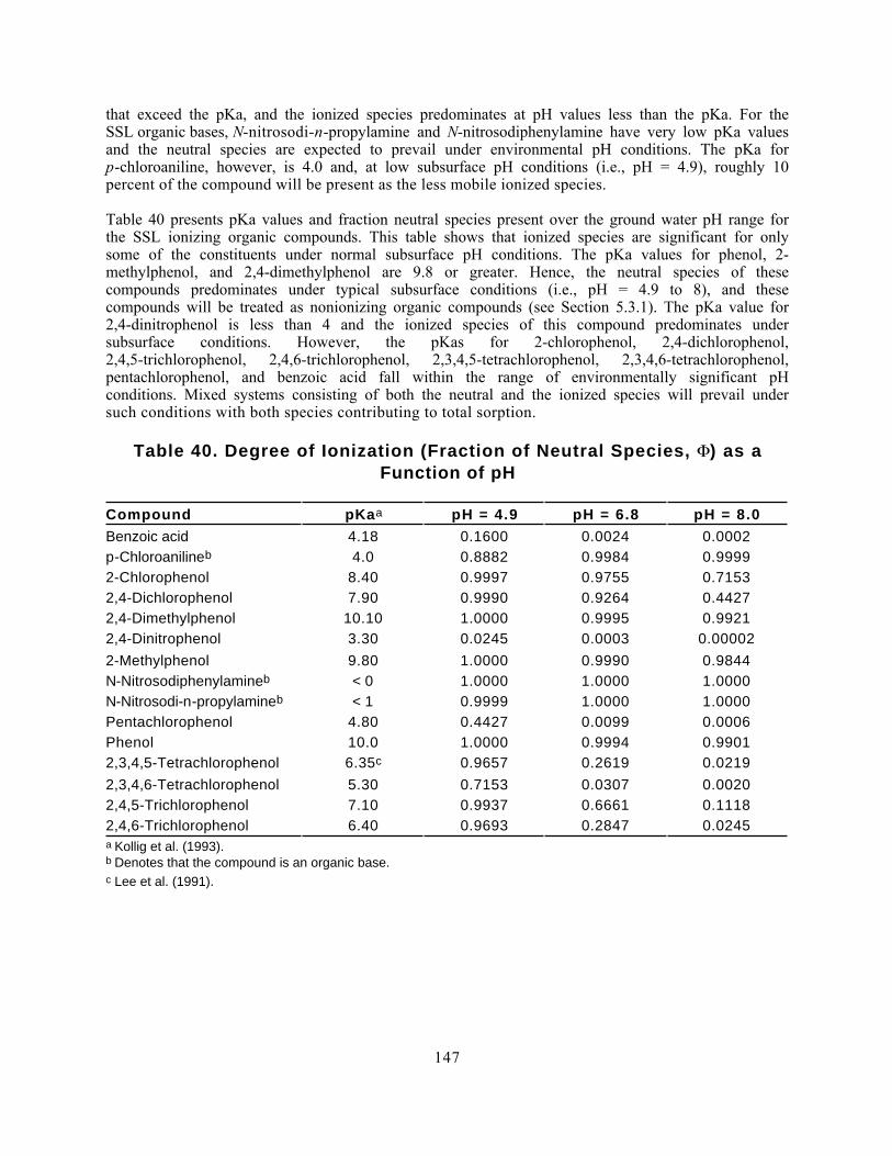
that exceed the pKa, and the ionized species predominates at pH values less than the pKa. For theSSL organic bases, N-nitrosodi-n-propylamine and N-nitrosodiphenylamine have very low pKa valuesand the neutral species are expected to prevail under environmental pH conditions. The pKa forp-chloroaniline, however, is 4.0 and, at low subsurface pH conditions (i.e., pH = 4.9), roughly 10percent of the compound will be present as the less mobile ionized species.
Table 40 presents pKa values and fraction neutral species present over the ground water pH range forthe SSL ionizing organic compounds. This table shows that ionized species are significant for onlysome of the constituents under normal subsurface pH conditions. The pKa values for phenol, 2-methylphenol, and 2,4-dimethylphenol are 9.8 or greater. Hence, the neutral species of thesecompounds predominates under typical subsurface conditions (i.e., pH = 4.9 to 8), and thesecompounds will be treated as nonionizing organic compounds (see Section 5.3.1). The pKa value for2,4-dinitrophenol is less than 4 and the ionized species of this compound predominates undersubsurface conditions. However, the pKas for 2-chlorophenol, 2,4-dichlorophenol,2,4,5-trichlorophenol, 2,4,6-trichlorophenol, 2,3,4,5-tetrachlorophenol, 2,3,4,6-tetrachlorophenol,pentachlorophenol, and benzoic acid fall within the range of environmentally significant pHconditions. Mixed systems consisting of both the neutral and the ionized species will prevail undersuch conditions with both species contributing to total sorption.
Table 40. Degree of Ionization (Fraction of Neutral Species, ) as aFunction of pH
Compound pKaa pH = 4.9 pH = 6.8 pH = 8.0
Benzoic acid 4.18 0.1600 0.0024 0.0002p-Chloroanilineb 4.0 0.8882 0.9984 0.99992-Chlorophenol 8.40 0.9997 0.9755 0.71532,4-Dichlorophenol 7.90 0.9990 0.9264 0.44272,4-Dimethylphenol 10.10 1.0000 0.9995 0.99212,4-Dinitrophenol 3.30 0.0245 0.0003 0.00002
2-Methylphenol 9.80 1.0000 0.9990 0.9844N-Nitrosodiphenylamineb < 0 1.0000 1.0000 1.0000N-Nitrosodi-n-propylamineb < 1 0.9999 1.0000 1.0000Pentachlorophenol 4.80 0.4427 0.0099 0.0006Phenol 10.0 1.0000 0.9994 0.99012,3,4,5-Tetrachlorophenol 6.35c 0.9657 0.2619 0.0219
2,3,4,6-Tetrachlorophenol 5.30 0.7153 0.0307 0.00202,4,5-Trichlorophenol 7.10 0.9937 0.6661 0.11182,4,6-Trichlorophenol 6.40 0.9693 0.2847 0.0245a Kollig et al. (1993).b Denotes that the compound is an organic base.c Lee et al. (1991).
147
Prediction of Soil-Water Partition Coefficients. Lee et al. (1990) developed arelationship from thermodynamic equilibrium considerations to predict the total sorption of anionizable organic compound from the partitioning of its ionized and neutral forms:
Koc = Koc,nΦn + Koc,i (1 - Φn) (74)
where
Koc = soil organic carbon/water partition coefficient (L/kg)Koc,n = partition coefficient for the neutral species (L/kg)Φn = fraction of neutral species present for acids or basesKoc,i = partition coefficient for the ionized species (L/kg).
This relationship defines the total sorption coefficient for any ionizing compound as the sum of theweighted individual sorption coefficients for the ionized and neutral species at a given pH. Lee et al.(1990) verified that this relationship adequately predicts laboratory-measured Koc values forpentachlorophenol.
A literature review was conducted to compile the pKa and the laboratory-measured values of Koc,n
and Koc,i shown in Table 41. Data collected during this review are presented in RTI (1994), alongwith the references reviewed. Sorption coefficients for both neutral and ionized species were reportedfor only four of the nine ionizable organic compounds of interest. Sorption coefficients reported forthe remaining compounds were generally Koc,n, and estimates of K oc,i were necessary to predict thecompound's total sorption. The methods for estimating Koc,i for organic acids and organic bases arediscussed separately in the following subsections.
Organic Acids. Sorption coefficients for both the neutral and ionized species have been reportedfor two chlorophenolic compounds: 2,4,6-trichlorophenol and pentachlorophenol. For 2,4,5-trichlorophenol and 2,3,4,5-tetrachlorophenol, soil-water partitioning coefficient (Kp) data in theliterature were adequate to allow calculation of Koc,i from Kp and soil foc (Lee et al., 1991). Fromthese measured values, the ratios of Koc,i to Koc,n are: 0.1 (2,4,6-trichlorophenol), 0.02(pentachlorophenol), 0.015 (2,4,5-trichlorophenol), and 0.051 (2,3,4,5-tetrachlorophenol). A ratioof 0.015 (1.5 percent) was selected as a conservative value to estimate Koc,i for the remainingphenolic compounds, benzoic acid, and vinyl acetate.
Organic Bases. No measured sorption coefficients for either the neutral or the ionized specieswere found for the three organic bases of interest (N-nitrosodi-n-propylamine,N-nitrosodiphenylamine, and p-chloroaniline). Generally, the sorption of ionizable organic bases hasnot been as well investigated as that of the organic acids, and there has been no relationshipdeveloped between the sorption coefficients of the neutral and ionized species. EPA is currentlyinitiating research on models for predicting the sorption of organic bases in the subsurface.
As noted earlier, the neutral species of the organic base predominates at pH values exceeding thepKa. For N-nitrosodi-n-propylamine (pKa < 1) and N-nitrosodiphenylamine (pKa < 0), the neutralspecies is present under environmentally significant conditions. The neutral species constitutesapproximately 90 percent of the system for p-chloroaniline (Table 40).
148

Table 41. Soil Organic Carbon/Water Partition Coefficients and pKaValues for Ionizing Organic Compounds
Compound Koc,n (L/kg) Koc,i (L/kg) pKaa
Benzoic acid 32b 0.5c 4.18
2-Chlorophenol 398b 6.0c 8.40
2,4-Dichlorophenol 159d 2.4c 7.90
2,4-Dinitrophenol 0.8a 0.01c 3.30
Pentachlorophenol 19,953e 398e 4.80
2,3,4,5-Tetrachlorophenol 17,916f 67g 6.35h
2,3,4,6-Tetrachlorophenol 6,190i 93c 5.30
2,4,5-Trichlorophenol 2,380i 36 j 7.10
2,4,6-Trichlorophenol 1,070i 107k 6.40a Kollig et al. (1993).b Meylan et al. (1992).c Estimate based on the ratio of Koc,i/Koc,n for compounds for which data exist; Koc,i was estimated to be 0.015 H
Koc,n .d Calculated using data (Kp = 0.62, foc = 0.0039) contained in Lee et al. (1991); agrees well with Boyd (1982)
reporting measured Koc = 126 L/kg.e Lee et al. (1990).f Average of values reported for two aquifer materials from Schellenberg et al. (1984).g Calculated using data (Kp = 0.26, foc = 0.0039) contained in Lee et al. (1991).h Lee et al. (1991).i Schellenberg et al. (1984).j Calculated using data (Kp = 0.14, foc = 0.0039) contained in Lee et al. (1991).k Kukowski (1989).
The neutral species has a lower tendency to sorb to subsurface materials than the positively chargedionized species. As a consequence, the determination of overall sorption potential based solely on theneutral species for N-nitrosodi-n-propylamine, N-nitrosodiphenylamine, and p-chloroaniline isconservative, and these three organic bases will be treated as nonionizing organic compounds (seeSection 5.3.1).
Soil-Water Partition Coefficients for Ionizing Organic Compounds. Partitioncoefficients for the neutral and ionized species (Koc,n and Koc,i, respectively) and pKa values for nineionizable organic compounds are provided in Table 41. These parameters can be used in Equation 74to compute Koc values for organic acids at any given pH. Koc values for each of the ionizablecompounds of interest are presented in Table 42 for pHs of 4.9, 6.8, and 8.0. Appendix L containspH-specific Koc values for ionizable organics over this entire range.
5.4 Soil-Water Distribution Coefficients (Kd) for Inorganic Constituents
As with organic chemicals, development of SSLs for inorganic chemicals (i.e., toxic metals) requires asoil-water partition coefficient (Kd) for each constituent. However, the simple relationship betweensoil organic carbon content and sorption observed for organic chemicals does not apply to inorganicconstituents. The soil-water distribution coefficient (Kd) for metals and other inorganic compounds isaffected by numerous geochemical parameters and processes, including pH; sorption to clays, organic
149

matter, iron oxides, and other soil constituents; oxidation/reduction conditions; major ion chemistry;and the chemical form of the metal. The number of significant influencing parameters, theirvariability in the field, and differences in experimental methods result in as much as seven orders ofmagnitude variability in measured metal Kd values reported in the literature (Table 43). Thisvariability makes it much more difficult to derive generic Kd values for metals than for organics.
Table 42. Predicted Soil Organic Carbon/Water Partition Coefficients(Koc,L/kg) as a Function of pH: Ionizing Organics
Compound pH = 4.9 pH = 6.8 pH = 8.0
Benzoic acid 5.5 0.6 0.5
2-Chlorophenol 398 388 2862,4-Dichlorophenol 159 147 72
2,4-Dinitrophenol 0.03 0.01 0.01Pentachlorophenol 9,055 592 410
2,3,4,5-Tetrachlorophenol 17,304 4,742 4582,3,4,6-Tetrachlorophenol 4,454 280 105
2,4,5-Trichlorophenol 2,365 1,597 2982,4,6-Trichlorophenol 1,040 381 131
Because of their great variability and a limited number of data points, no meaningful estimate ofcentral tendency Kd values for metals could be derived from available measured values. For thisreason, an equilibrium geochemical speciation model (MINTEQ) was selected as the best approachfor estimating Kd values for the variety of environmental conditions expected to be present atSuperfund sites.
This approach and model were also used by OSW to estimate generic Kd values for metals proposedfor use in the HWIR proposal (U.S. EPA, 1992a). The HWIR MINTEQA2 analyses were conductedunder a variety of geochemical conditions and metal concentrations representative of solid wastelandfills across the Nation. The metal Kd values developed for this effort were reviewed for SSLapplication and were used as preliminary values to develop the September 1993 draft SSLs.
Upon further review of the HWIR MINTEQ modeling effort, EPA decided it was necessary toconduct a separate MINTEQ modeling effort to develop metal Kd values for SSL application.Reasons for this decision include the following:
• It was necessary to expand the modeling effort to include other metal contaminantslikely to be encountered at Superfund sites (i.e., beryllium, copper, and zinc).
• HWIR work incorporated low, medium, and high concentrations of dissolved organicacids that are present in municipal solid waste (MSW) leachate. These organic acidsare not expected to exist in high concentrations in pore waters underlying Superfundsites; therefore, their inclusion in the Superfund contaminated soil scenario is notwarranted.
• The HWIR modeling simulations for chromium (+3) were found to be in error. Thiserror has been corrected in subsequent HWIR modeling work but corrected resultswere not available at the time of preliminary SSL development.
150

Table 43. Summary of Collected Kd Values Reported in Literature
AECL(1990)a
Baes and Sharp (1983) orBaes et al . (1984)b
Coughtrey etal . (1985)c
Battelle(1989)d
Metal RangeGeometric
Meane Range No. Values Range Range
Antimony 45-550 45f -- -- -- 2.0-15.9Arsenice -- 200f -- -- -- 5.86-19.4Arsenic (+3) -- 3.3g 1.0-8.3 19 -- --Arsenic (+5) -- 6.7g 1.9-18 37 -- --Barium -- 60f -- -- -- 530-16,000Beryllium 250-3,000 650f -- -- -- 70-8,000
Cadmium 2.7-17,000 6.4h 1.26-26.8 28 32-50 14.9-567Chromium 1.7-2,517 850f -- -- -- --Chromium (+2) -- 2,200g 470-150,000 15 -- --Chromium (+3) -- -- -- -- -- 168-3,600Chromium (+6) -- 37g 1.2-1,800 18 -- 16.8-360Mercurye -- 10f -- -- -- 322-5,280
Nickel 60-4,700 150f -- -- ~20 12.2-650Selenium 150-1,800 300f -- -- < 9 5.9-14.9Silver 2.7-33,000 46h 10-1,000 16 50 0.4-40.0Thallium -- 1,500f -- -- -- 0.0-0.8Vanadium -- 1,000f -- -- -- 50-100.0Zinc 0.1-100,000 38h 0.1-8,000 146 ≥ 20 --a The Atomic Energy of Canada, Limited (AECL, 1990) presents the distribution of Kd values according to four major
soil types—sand, silt, clay, and organic material. Their data were obtained from available literature. b Baes et al. (1984) present Kd values for approximately 220 agricultural soils in the pH range of 4.5 to 9. Their data
were derived from available literature and represent a diverse mixture of soils, extracting solutions, and laboratorytechniques.
c Coughtrey et al. (1985) report best estimates and ranges of measured soil Kd values for a limited number of metals. d Battelle Memorial Institute (Battelle, 1989) reports a range in Kd values as a function of pH (5 to 9) and sorbent
content (a combination of clay, aluminum and iron oxyhydroxides, and organic matter content). The sorbentcontent ranges were <10 percent, 10 to 30 percent, and >30 percent sorbent. Their data were based on availableliterature.
e The valence of these metals is not reported in the documents.f Estimated based on the correlation between Kd and soil-to-plant concentration factor (Bv).g Average value reported by Baes and Sharp (1983).h Represents the median of the logarithms of the observed values.
For these reasons, a MINTEQ modeling effort was expanded to develop a series of metal-specificisotherms for several of the metals expected to be present in soils underlying Superfund sites. Themodel used was an updated version of MINTEQA2 obtained from Allison Geoscience Consultants,Inc. Model results are reported in the December 1994 draft Technical Background Document (U.S.EPA, 1994i) and were used to calculate the SSLs presented in the December 1994 draft Soil ScreeningGuidance (U.S. EPA, 1994h).
151

The MINTEQA2 model was further updated by Allison Geoscience Consultants, Inc., in 1995 toinclude thermodynamic data for silver, an improved estimate of water saturation in the vadose zone(i.e., water saturation is assumed to be 77.7 percent saturated as opposed to 100 percent), and revisedestimates of sorbent mass (i.e., organic matter content, iron oxide content).
This updated model, which is expected to be made public through EPA’s Environmental ResearchLaboratory in Athens, Georgia, was used to revise the generic Kd values for the EPA/OSW HWIRmodeling effort. The metal Kd values for SSL application were also revised. Model results arecontained in this document. The following section describes the important assumptions andlimitations of this modeling effort.
5.4.1 Modeling Scope and Approach. New MINTEQA2 modeling runs wereconducted to develop sorption isotherms for barium, beryllium, cadmium, chromium (+3), copper,mercury (+2), nickel, silver, and zinc. The general approach and input values used for pH, iron oxide(FeOx) concentration, and background chemistry were unchanged from the HWIR modeling effort.
The HWIR MINTEQA2 analyses were conducted under a variety of geochemical conditions andmetal concentrations. Three types of parameters were identified as part of the chemical speciationmodeling effort: (1) parameters that have a direct first-order impact on metal speciation and arecharacterized by a wide range in environmental variability; (2) parameters that have an indirect,generally less pronounced effect on metal speciation and are characterized by a relatively small orinsignificant environmental variability; and (3) parameters that may have a direct first-order impacton metal speciation but neither the natural variability nor its significance is known.
In the HWIR modeling effort, parameters of the first type ("master variables") were limited to thosehaving a significant effect on model results, including pH, concentration of available amorphous ironoxide adsorption sites (i.e., FeOx content), concentration of solid organic matter adsorption sites(with a dependent concentration of dissolved natural organic matter), and concentration of leachateorganic acids expected to be present in MSW leachate. High, medium, and low values were assigned toeach of the master variables to account for their natural environmental variability. The SSLmodeling effort used this same approach and inputs except that anthropogenic organic acids were notincluded in the model simulations. Furthermore, the SSL modeling effort incorporated a mediumfraction of organic carbon (foc) that correlated to the HWIR high concentration.
Parameters of the second type constitute the background pore-water chemistry, which consists ofchemical constituents commonly occurring in ground water at concentrations great enough to affectmetal speciation. These constituents were treated as constants in both the SSL and HWIR effort. Thethird type of parameter was entirely omitted from consideration in both modeling efforts due topoorly understood geochemistry and the lack of reliable thermodynamic data. The most importantof these parameters is the oxidation-reduction (redox) potential. To compensate, both modelingefforts incorporated an approach that was most protective of the environment with respect to theimpact of redox potential on the partitioning of redox-sensitive metals (i.e., each metal was modeledin the oxidation state that most enhances metal mobility).
For the HWIR modeling effort, metal concentrations were varied from the maximum contaminantlevel (MCL) to 1,000 times the MCL for each individual metal. This same approach was taken forSSL modeling, although for certain metals the concentration range was extended to determine themetal concentration at which the sorption isotherm departed from linearity.
Sorption isotherms for arsenic (+3), chromium (+6), selenium, and thallium are unchanged from theprevious efforts and are based on laboratory-derived pH-dependent sorption relationships developed
152

for HWIR. Using these relationships, the Kd distribution as a function of pH is presented for each ofthese four metals in Figure 10.
Sorption isotherms for antimony and vanadium could not be estimated using MINTEQA2 because thethermodynamic databases do not contain the required reactions and associated equilibrium constants.Sufficient experimental research has not been conducted to develop pH-dependent relationships forthese two metals. As a consequence, Kd values for antimony and vanadium were obtained from Baeset al. (1984) (Table 43). These Kd values are not pH-dependent.
5.4.2 Input Parameters. Table 44 lists high, medium, and low values for pH and iron oxideused for both the HWIR and SSL MINTEQ modeling efforts. Sources for these values are as follows(U.S. EPA, 1992a):
• Values for pH were obtained from analysis of 24,921 field-measured pH valuescontained in the EPA STORET database. The pH values of 4.9, 6.8, and 8.0correspond to the 7.5th, 50th, and 92.5th percentiles of the distribution.
• Iron oxide contents were based on analysis of six aquifer samples collected over awide geographic area, including Florida, New Jersey, Oregon, Texas, Utah, andWisconsin. The lowest of the six analyses was taken to be the low value, the averageof the six was used as the medium value, and the highest was taken as the high value.
The development of the values presented in Table 44 is described in more detail in U.S. EPA(1992a).
Thirteen chemical constituents commonly occurring in ground water were used to define thebackground pore-water chemistry for HWIR and SSL modeling efforts (Table 45). Because theseconstituents were treated as constants, a single total ion concentration, corresponding to the mediantotal metal concentration from a probability distribution obtained from the STORET database, wasassigned to each of the background pore-water constituents (U.S. EPA, 1992a).
Although the HWIR and the SSL MINTEQ modeling efforts were consistent in the majority of theassumptions and input parameters used, the fraction of organic carbon (foc) used for the SSL modelingeffort was slightly different than that used for the HWIR modeling effort. The foc used for the SSLeffort was equal to 0.002 g/g, which better reflected average subsurface conditions at Superfund sites.This value is approximately equal to the high value of organic carbon used in the HWIR modelingeffort.
Table 44. Summary of Geochemical Parameters Used in SSL MINTEQModeling Effort
Value pH Iron oxide content (weight percent)Low 4.9 0.01
Medium 6.8 0.31High 8.0 1.11
Source: U.S. EPA (1992a)
153

Figure 10. Empirical pH-dependent adsorption relationship: arsenic (+3), chromium
0
0.5
1
1.5
2
2.5
3.5 4 4.5 5 5.5 6 6.5 7 7.5 8 8.5 9 9.5
pH
log
Kd (
L/k
g)
Chromium (+6)
Arsenic (+3)
Selenium
Thallium
154

Table 45. Background Pore-Water Chemistry Assumed for SSL MINTEQModeling Efforta
Parameter Concentration (mg/L)
Aluminum 0.2Bromine 0.3Calcium 48
Carbonate 187Chlorine 15Iron (+3) 0.2
Magnesium 14Manganese (+2) 0.04
Nitrate 1Phosphate 0.09Potassium 2.9b
Sodium 22
Sulfate 25a Median values from STORET database as reported in U.S. EPA (1992a).b Median values from STORET database; personal communication from J.
Allison, Allison Geosciences.
5.4.3. Assumptions and Limitations. The SSL MINTEQ modeling effort incorporatesseveral basic simplifying assumptions. In addition, the applicability and accuracy of the model resultsare subject to limitations. Some of the more significant assumptions and limitations are describedbelow.
• The system is assumed to be at equilibrium. This assumption is inherent ingeochemical aqueous speciation models because the fundamental equations of massaction and mass balance are equilibrium based. Therefore, any possible influence ofadsorption (or desorption) rate limits is not considered.
This assumption is conservative. Because the model is being used to simulate metaldesorption from the solid substrate, if equilibrium conditions are not met, thedesorption reaction will be incomplete and the metal concentration in pore water willbe less than predicted by the model.
• Redox potential is not considered. The redox potential of the system is notconsidered due to the difficulty in obtaining reliable field measurements of oxidationreduction potential (Eh), which are needed to determine a realistic frequencydistribution of this parameter. Furthermore, the geochemistry of redox-sensitivespecies is poorly understood. Reactions involving redox species are often biologicallymediated and the concentrations of redox species are not as likely to reflectthermodynamic equilibrium as other inorganic constituents.
To provide a conservative estimate of metal mobility, all environmentally viableoxidation states are modeled separately for the redox-sensitive metals; the mostconservative was selected for defining SSL metal Kd values. The redox-sensitive
155

constituents that make up the background chemistry are represented only by theoxidation state that most enhances metal mobility (U.S. EPA, 1992a).
• Potential sorbent surfaces are limited. Only metal adsorption to FeOx and solidorganic matter is considered in the system. It is recognized that numerous othernatural sorbents exist (e.g., clay and carbonate minerals); however, thermodynamicdatabases describing metal adsorption to these surfaces are not available and thepotential for adsorption to such surfaces is not considered. This assumption isconservative and will underpredict sorption for soils with significant amounts of suchsorption sites.
• The available thermodynamic database is limiting. As metal behavior increasesin complexity, thermodynamic data become more rare. The lack of completethermodynamic data requires simplification to the defined system. This simplificationmay be conservative or nonconservative in terms of metal mobility.
• Metal competition is not considered. Model simulations were performed forsystems comprised of only one metal (i.e., the potential for competition betweenmultiple metals for available sorbent surface sites was not considered). Generally, thecompetition of multiple metals for available sorption sites results in higher dissolvedmetal concentrations than would exist in the absence of competition. Consequently,this assumption is nonconservative but is significant only at metal concentrationsmuch higher than the SSLs.
Other assumptions and limitations associated with this modeling effort are discussed in RTI (1994).
5.4.4 Results and Discussion. MINTEQ model results indicate that metal mobility ismost affected by changes in pH. Based on this observation and because iron oxide content is notroutinely measured in site characterization efforts, pH-dependent Kds for metals were developed forSSL application by fixing iron oxide at its medium value and fraction organic carbon at 0.002. Forarsenic (+3), chromium (+6), selenium, and thallium, the empirical pH-dependent Kds were used.
Table 46 shows the SSL Kd values at high, medium, and low subsurface pH conditions. Figure 11 plotsMINTEQ-derived metal Kd values over this pH range. Figure 10 shows the same for the empiricallyderived metal Kds. These results are discussed below by metal and compared with measured values. SeeRTI (1994) for more information. pH-dependent values are not available for antimony, cyanide, andvanadium. The estimated Kd values shown in Table 46 for antimony and vanadium are reported byBaes et al. (1984) and the Kd value for cyanide is obtained from SCDM.
Arsenic. Kd values developed using the empirical equation for arsenic (+3) range from 25 to 31L/kg for pH values of 4.9 to 8.0, respectively. These values correlate fairly well with the range ofmeasured values reported by Battelle (1989)—5.86 to 19.4 L/kg. They are slightly above the rangereported by Baes and Sharp (1983) for arsenic (+3) (1.0-8.3). The estimated Kd values for arsenic(+3) do not correlate well with the value of 200 L/kg presented by Baes et al. (1984). Oxidation stateis not specified in Baes et al. (1984), and the difference between the empirical-derived Kd valuespresented here and the value presented by Baes et al. (1984) may reflect differences in oxidationstates (arsenic (+3) is the most mobile species).
156

Note: Conditions depicted are medium iron oxide content (0.31 wt %) and organic matter of 0.2 wt %.
Figure 11. Metal Kd as a function of pH.
0
1
2
3
4
5
6
7
3.5 4.0 4.5 5.0 5.5 6.0 6.5 7.0 7.5 8.0 8.5
pH
log
Kd (
L/k
g)
Chromium (+3)
Cadmium
Beryllium
Nickel
-3
-2
-1
0
1
2
3
3.5 4.0 4.5 5.0 5.5 6.0 6.5 7.0 7.5 8.0 8.5
pH
log
Kd (
L/k
g) Zinc
Barium
Silver
Mercury
Zinc
Barium
SilverMercury
157

Table 46. Estimated Inorganic Kd Values for SSL Application
Estimated Kd (L/kg)
Metal pH = 4.9 pH = 6.8 pH = 8.0
Antimonya 4.5E+01Arsenic (+3)b 2.5E+01 2.9E+01 3.1E+01Barium 1.1E+01 4.1E+01 5.2E+01Beryllium 2.3E+01 7.9E+02 1.0E+05Cadmium 1.5E+01 7.5E+01 4.3E+03
Chromium (+3) 1.2E+03 1.8E+06 4.3E+06Chromium (+6)b 3.1E+01 1.9E+01 1.4E+01Cyanidec 9.9E+00Mercury (+2) 4.0E-02 5.2E+01 2.0E+02Nickel 1.6E+01 6.5E+01 1.9E+03Seleniumb 1.8E+01 5.0E+00 2.2E+00
Silver 1.0E-01 8.3E+00 1.1E+02Thalliumb 4.4E+01 7.1E+01 9.6E+01Vanadiuma 1.0E+03Zinc 1.6E+01 6.2E+01 5.3E+02a Geometric mean measured value from Baes et al., 1984 (pH-dependent values not available).b Determined using an empirical pH-dependent relationship (Figure 10).c SCDM = Superfund Chemical Data Matrix (pH-dependent values not available).
Barium. For ground water pH conditions, MINTEQ-estimated Kd values for barium range from 11to 52 L/kg. This range correlates well with the value of 60 L/kg reported by Baes et al. (1984).Battelle (1989) reports a range in Kd values from 530 to 16,000 L/kg for a pH range of 5 to 9. Themodel-predicted Kd values for barium are several orders of magnitude less than the measured values,possibly due to the lower sorptive potential of iron oxide, used as the modeled sorbent, relative toclay, a sorbent present in the experimental systems reported by Battelle (1989).
Beryllium. The Kd values estimated for beryllium range from 23 to 100,000 L/kg for theconditions studied. AECL (1990) reports medians of observed values for Kd ranging from 250 L/kgfor sand to 3,000 L/kg for organic matter. Baes et al. (1984) report a value of 650 L/kg. Battelle(1989) reports a range of Kd values from 70 L/kg for sand to 8,000 L/kg for clay. MINTEQ resultsfor medium ground water pH (i.e., a value of 6.8) yields a Kd value of 790 L/kg. Hence, there isreasonable agreement between the MINTEQ-predicted Kd values and values reported in the literature. Cadmium. For the three pH conditions, MINTEQ Kd values for cadmium range from 15 to 4,300L/kg, with a value of 75 at a pH of 6.8. The range in experimentally determined Kd values forcadmium is as follows: 1.26 to 26.8 L/kg (Baes et al., 1983), 32 to 50 L/kg (Coughtrey et al., 1985),14.9 to 567 L/kg (Battelle, 1989), and 2.7 to 17,000 L/kg (AECL, 1990). Thus the MINTEQestimates are generally within the range of measured values.
Chromium (+3). MINTEQ-estimated Kd values for chromium (+3) range from 1,200 to4,300,000 L/kg. Battelle (1989) reports a range of Kd values of 168 to 3,600 L/kg, orders of
158

magnitude lower than the MINTEQ values. This difference may reflect the measurements of mixedsystems comprised of both chromium (+3) and (+6). The incorporation of chromium (+6) would tendto lower the Kd. Because the model-predicted values may overpredict sorption, the user shouldexercise care in the use of these values. Values for chromium (+6) should be used where speciation ismixed or uncertain.
Chromium (+6). Chromium (+6) Kd values estimated using the empirical pH-dependentadsorption relationship range from 31 to 14 L/kg for pH values of 4.9 to 8.0. Battelle (1989) reportsa range of 16.8 to 360 L/kg for chromium (+6) and Baes and Sharp (1983) report a range of 1.2 to1,800. The predicted chromium (+6) Kd values thus generally agree with the lower end of the rangeof measured values and the average measured values (37) reported by Baes and Sharp (1983). Thesevalues represent conservative estimates of mobility the more toxic of the chromium species.
Mercury (+2). MINTEQ-estimated Kd values for mercury (+2) range from 0.04 to 200 L/kg.These model-predicted estimates are less than the measured range of 322 to 5,280 L/kg reported byBattelle (1989). This difference may reflect the limited thermodynamic database with respect tomercury and/or that only the divalent oxidation state is considered in the simulation. Allison (1993)reviewed the model results in comparison to the measured values reported by Battelle (1989) andfound reasonable agreement between the two sets of data, given the uncertainty associated withlaboratory measurements and model precision.
Nickel. MINTEQ-estimated Kd values for nickel range from 16 to 1,900 L/kg. These values agreewell with measured values of approximately 20 L/kg (mean) and 12.2 to 650 L/kg, reported byCoughtrey et al. (1985) and Battelle (1989), respectively. These values also agree well with the valueof 150 L/kg reported by Baes et al. (1984). However, the predicted values are at the low end of therange reported by the AECL (1990)—60 to 4,700 L/kg.
Selenium . Empirically derived Kd values for selenium range from 2.2 to 18 L/kg for pH values of8.0 to 4.9. The range in experimentally determined Kd values for selenium is as follows: less than 9L/kg (Coughtrey et al., 1985), 5.9 to 14.9 L/kg (Battelle, 1989), and 150 to 1,800 L/kg (AECL,1990). Baes et al. (1984) reported a value of 300 L/kg. Although they are significantly below thevalues presented by the AECL (1990) and Baes et al. (1984), the MINTEQ-predicted Kd valuescorrelate well with the values reported by Coughtrey et al. (1985) and Battelle (1989).
Silver . The Kd values estimated for silver range from 0.10 to 110 L/kg for the conditions studied.The range in experimentally determined Kd values for silver is as follows: 2.7 to 33,000 L/kg (AECL,1990), 10 to 1,000 L/kg (Baes et al., 1984), 50 L/kg (Coughtrey et al., 1985), and 0.4 to 40 L/kg(Battelle, 1989). The model-predicted Kd values agree well with the values reported by Coughtrey etal. (1985) and Battelle (1989) but are at the lower end of the ranges reported by AECL (1990) andBaes et al. (1984).
Thallium. Empirically derived Kd values for thallium range from 44 to 96 L/kg for pH values of4.9 to 8.0. Generally, these values are about an order of magnitude greater than those reported byBattelle (1989)—0.0 to 0.8 L/kg - but are well below the value predicted by Baes et al. (1984).
Zinc. MINTEQ-estimated Kd values for zinc range from 16 to 530 L/kg. These estimated Kd valuesare within the range of measured Kd values reported by the AECL (1990) (0.1 to 100,000 L/kg) andBaes et al. (1984) (0.1 to 8,000 L/kg). Coughtrey et al. (1985) reported a Kd value for zinc ofgreater than or equal to 20 L/kg.
159

5.4.5 Analysis of Peer-Review Comments. A peer review was conducted of themodel assumptions and inputs used to estimate Kd values for SSL application. This review identifiedseveral issues of concern, including:
• The charge balance exceeds an acceptable margin of difference (5 percent) in most ofthe simulations. A variance in excess of 5 percent may indicate that the modelproblem is not correctly chemically poised and therefore the results may not bechemically meaningful.
• The model should not allow sulfate to adsorb to the iron oxide. Sulfate is a weaklyouter-sphere adsorbing species and, by including the adsorption reaction, sulfate isremoved from the aqueous phase at pH values less than 7 and is prevented fromparticipating in precipitation reaction at these pH values.
• Modeled Kd values for barium and zinc could not be reproduced for all studiedconditions.
A technical analysis of these concerns indicated that, although these comments were based on trueobservations about the model results, these factors do not compromise the validity of the MINTEQresults in this application. This technical analysis is provided in Appendix M.
160

Part 6: REFERENCES
Abdul, A.S., T.L. Gibson, and D.N. Rai. 1987. Statistical correlations for predicting the partitioncoefficient for nonpolar organic contaminants between aquifer carbon and water. HazardousWaste and Hazardous Materials 4(3):211-223.
AECL (Atomic Energy of Canada Limited). 1990. A Critical Compilation and Review of Default SoilSolid/Liquid Partition Coefficients, Kd, for Use in Environmental Assessments, by D.H.Thibault, M.I. Sheppard, and P.A. Smith, Whiteshell Nuclear Research Establishment,Pinawa, Manitoba.
Aller, L., T. Bennett, J.H. Lehr, R.J. Petty, and G. Hackett. 1987. DRASTIC: A Standardized Systemfor Evaluating Ground Water Pollution Potential Using Hydrogeologic Settings. EPA-600/2-87-035. Prepared for U.S. EPA Office of Research and Development, Ada, OK. NationalWater Well Association, Dublin, OH.
Allison, J. 1993. Review and Evaluation of the MINTEQA2 Kd Results for Mercury in the FiniteSource Methodology. Prepared by Allison Geoscience Consultants, Inc., for the U.S.Environmental Protection Agency, Environmental Research Laboratory, Athens, GA.
ASTM (American Society for Testing and Materials). 1994. Risk-Based Corrective Action Guidance.Philadelphia, PA. (Draft).
Baes, C.F. (III), and R.D. Sharp. 1983. A proposal for estimation of soil leaching and leachingconstants for use in assessment models. J. Environ. Qual. 12(1):17-28.
Baes, C.F. (III), R.D. Sharp, A.L. Sjoreen, and R.W. Shor. 1984. A Review and Analysis ofParameters for Assessing Transport of Environmentally Released Radionuclides throughAgriculture. Oak Ridge National Laboratory Report ORNL-5786. ORNL, Oak Ridge, TN.
Battelle Memorial Institute. 1989. Chemical Data Bases for the Multimedia Environmental PollutantAssessment System (MEPAS): Version 1. Prepared for the U.S. Department of Energy underContract DE-AC06-76RKI 1830, by Pacific Northwest Laboratory, operated by BattelleMemorial Institute.
Boyd, S.A. 1982. Adsorption of substituted phenols by soil. Soil Science, 134(5):337-343.
Brady, N.C. 1990. The Nature and Properties of Soils. Macmillan Publishing Company, New York,NY.
Calabrese, E.J., H. Pastides, R. Barnes, et al. 1989. How much soil do young children ingest: anepidemiologic study. In: Petroleum Contaminated Soils , Vol. 2. E.J. Calabrese and P.T.Kostecki, eds. pp. 363-417. Chelsea, MI, Lewis Publishers.
Carsel, R.F., and R.S. Parrish. 1988. Developing joint probability distributions of soil water retentioncharacteristics. Water Resources Research, 24(5):755-769.
161

Carsel, R.F., R.S. Parrish, R.L. Jones, J.L. Hansen, and R.L. Lamb. 1988. Characterizing theuncertainty of pesticide leaching in agricultural soils. J. of Contam. Hyd. 2:111-124.
Chen, L. 1995. Testing the mean of skewed distributions. Journal of the American StatisticalAssociation 90(430):767-772.
Coughtry, P.J., D. Jackson, and M.C. Thorne. 1985. Radionuclide Distribution and TransportingTerrestrial and Aquatic Ecosystems: A Compendium of Data. A.A. Balkem, Netherlands,Vol. 6.
Cowherd, C., G. Muleski, P. Engelhart, and D. Gillette. 1985. Rapid Assessment of Exposure toParticulate Emissions from Surface Contamination. EPA/600/8-85/002. NTIS PB85-192219. Office of Health and Environmental Assessment, U.S. Environmental ProtectionAgency, Washington, DC.
Criscenti, L.J., S.B. Christian, E.Z. Hosseinipour, and V.M. Gorokhovski. 1994. Evaluation ofUnsaturated Zone/Vadose Zone Models for Superfund Sites. Draft Report. EnvironmentalResearch Laboratory, Office of Research and Development, U.S. Environmental ProtectionAgency, Athens, GA.
Curtis, G. P., P. V. Roberts, and M. Reinhard. 1986. A natural gradient experiment on solutetransport in a sand aquifer. Water Resources Research 22(13):2059-2067.
Davis, S., P. Waller, R. Buschom, J. Ballou, and P. White. 1990. Quantitative estimates of soilingestion in normal children between the ages of 2 and 7 years: population-based estimatesusing Al, Si, and Ti as soil tracer elements. Archives of Environmental Health 45:112-122.
Di Toro, D.M. 1985. A particle interaction model of reversible organic chemical sorption.Chemosphere 14(10):1503-1538.
Dragun, J. 1988. The Soil Chemistry of Hazardous Materials . Hazardous Materials Control ResearchInstitute, Silver Spring, MD.
EQ (Environmental Quality Management). 1992. Limited Validation of the Hwang and Falco Modelfor Emissions of Soil-Incorporated Volatile Organic Compounds. Contract No. 68-D8-0111.Prepared for Office of Emergency and Remedial Response, U.S. Environmental ProtectionAgency, Washington, DC.
EQ (Environmental Quality Management). 1993. Evaluation of the Dispersion Equations in the RiskAssessment Guidance for Superfund (RAGS): Volume I—Human Health Evaluation Manual(Part B, Development of Preliminary Remediation Goals). Contract No. 68-02-D120.Prepared for Office of Emergency and Remedial Response, U.S. Environmental ProtectionAgency, Washington, DC.
EQ (Environmental Quality Management). 1994. Revisions to VF and PEF Equations. Memorandum#5099-3. Prepared for Office of Emergency and Remedial Response, U.S. EnvironmentalProtection Agency, Washington, DC.
EQ (Environmental Quality Management) and Pechan (E. H. Pechan and Associates). 1994. AComparison of Soil Volatilization Models in Support of Superfund Soil Screening LevelDevelopment. Contract No. 68-D3-0035. Prepared for Office of Emergency and RemedialResponse, U.S. Environmental Protection Agency, Washington, DC.
162

EQ (Environmental Quality Management). 1995. Limited Validation of the Jury Infinite Source andJury Reduced Solution Finite Source Models for Emissions of Soil-Incorporated VolatileOrganic Compounds. Prepared for Office of Solid Waste and Emergency Response, U.S.Environmental Protection Agency, Washington, DC.
Farmer, W. J., and J. Letey. 1974. Volatilization Losses of Pesticides from Soils . EPA-660/2-74/054.Office of Research and Development, U.S. Environmental Protection Agency, Washington,DC.
Feenstra, S., D.M. MacKay, and J.A. Cherry. 1991. A method for assessing residual NAPL based onorganic chemical concentrations in soil samples. Ground Water Monitoring Rev. 11(2):128-136.
Gee, G.W., and J.W. Bauder. 1986. Particle size analysis. In: A. Klute (ed.), Methods of Soil Analysis.Part 1. Physical and Mineralogical Methods. 2nd Edition, 9(1):383-411, American Societyof Agronomy, Madison, WI.
Gelhar, L.W., and C.J. Axness. 1981. Stochastic Analysis of Macro-Dispersion in Three-Dimensionally Heterogeneous Aquifers. Report No. H-8. Hydraulic Research Program. NewMexico Institute of Mining and Technology, Socorro, NM.
Gilbert, Richard O. 1987. Statistical Methods for Environmental Pollution Monitoring. New York:Van Nostrand Reinhold.
Hardin, J.W., and R.O. Gilbert. 1993. Comparing Statistical Tests for Detecting Soil ContaminationGreater than Background. Pacific Northwest Laboratory (PNL-8989), Richard, WA.
Heath, R.C. 1984. Ground-Water Regions of the United States. USGS Water Supply Paper 2242. U.S.Geological Survey, Reston, VA.
Howard, P. H. 1989. Handbook of Environmental Fate and Exposure Data for Organic Chemicals.Vol. I. Large Production and Priority Pollutants. Lewis Publishers, Chelsea, MI.
Hwang, S. T., and J. W. Falco. 1986. Estimation of Multimedia Exposure Related to Hazardous Waste
Facilities. Y. Cohen, Ed. Plenum Publishing.
Johnson, N.L. 1978. Modified t tests and confidence intervals for asymmetrical populations. Journalof the American Statistical Association 73(363):536-544.
Johnson, P.C. and R.A. Ettinger. 1991. Heuristic model for predicting the intrusion rate ofcontaminant vapors into buildings. Environmental Science and Technology 25(8):1445-1452.
Jury, W.A., W.F. Spencer, and W.J. Farmer. 1983. Behavior assessment model for trace organics insoil: I. Model description. J. Environ. Qual. 12(4):558-564.
Jury, W.A., W.J. Farmer, and W.F. Spencer. 1984. Behavior assessment model for trace organics insoil: II. Chemical classification and parameter sensitivity. J. Environ. Qual. 13(4):567-572.
Jury, W.A., D. Russo, G. Streile, and H.E. Abd. 1990. Evaluation of volatilization by organicchemicals residing below the soil surface. Water Resources Research 26(1):13-20.
Karickhoff, S.W. 1984. Organic pollutant sorption in aquatic systems. J. Hydraul. Eng . 110(6):707-735.
163
Kollig, H.P. 1993. Environmental Fate Constants for Organic Chemicals under Consideration forEPA's Hazardous Waste Identification Projects. Office of Research and Development, U.S.Environmental Protection Agency, Washington, DC.
Kukowski, H. 1989. Adsorption and Desorption of Ionizable Organic Chemicals by Soils. Ph.D.Dissertation, University of Kiel.
Land, C.E. 1971. Confidence intervals for linear functions of the normal mean and variance. Annalsof Mathematical Statistics 42:1187-1205.
Land, C.E. 1975. Tables of confidence limits for linear functions of the normal mean and variance.Selected Tables in Mathematical Statistics, 3:385-419. American Mathematical Society,Providence, RI.
Lee, L. S., P. S. C. Rao, P. Nkedi-Kizza, and J. J. Delfino. 1990. Influence of solvent and sorbentcharacteristics on distribution of pentachlorophenol in octanol-water and soil-water systems.Environ. Sci. Tech. 24:654-661.
Lee, L. S., P. S. C. Rao, and M. L. Brusseau. 1991. Nonequilibrium sorption and transport of neutraland ionized compounds. Environ. Sci. Tech. 25:722-729.
Lyman, W. J., W. F. Reehl, and D. H. Rosenblatt. 1982. Handbook of Chemical Property EstimationMethods. McGraw-Hill, New York.
Marshall, J. 1971. Drag measurements in roughness arrays of varying density and distribution.Agricultural Meteorology, 8:269-292.
McCarty, P.L., M. Reinhard, and B.E. Rittmann. 1981. Trace organics in ground water. Environ. Sci.Technol. 15:40-51.
McLean, E.O. 1982. Soil pH and lime requirement. In: A.L. Page (ed.), Methods of Soil Analysis.Part 2. Chemical and Microbiological Properties. 2nd Edition, 9(2):199-224, AmericanSociety of Agronomy, Madison, WI.
Meylan, W., P.H. Howard, and R.S. Boethling. 1992. Molecular topology/fragment contributionmethod for predicting soil sorption coefficients. Environ. Sci. Technol. 26(8):1560-1567.
Miller, R.G. 1991. Simultaneous Statistical Inference. 2nd edition. Springer-Verlag, New York.
Millington, R. J., and J. M. Quirk. 1961. Permeability of porous soils. Trans. Faraday Soc. 57:1200-1207.
Nelson, D.W., and L.E. Sommers. 1982. Total carbon, organic carbon, and organic matter. In: A.L.Page (ed.), Methods of Soil Analysis. Part 2. Chemical and Microbiological Properties. 2ndEdition, 9(2):539-579, American Society of Agronomy, Madison, WI.
Newell, C.J., L.P. Hopkins, and P.B. Bedient. 1989. Hydrogeologic Database for Ground WaterModeling. API Publication No. 4476. American Petroleum Institute, Washington, DC.
Newell, C.J., L.P. Hopkins, and P.B. Bedient. 1990. A hydrogeologic database for ground water-modeling. Ground Water, 28(5):703-714.
164

Nofziger, D.L., J. Chen, and C.T. Haan. 1994. Evaluation of Unsaturated/Vadose Zone Models forSuperfund Sites. EPA/600/R-93/184. Office of Research and Development, U.S.Environmental Protection Agency, Robert S. Kerr Environmental Research Laboratory, Ada,OK.
Piwoni, M. D., and P. Banerjee. 1989. Sorption of volatile organic solvents from aqueous solutiononto subsurface solids. J. Contam. Hydrol. 4(2):163-179.
Radian. 1989. Short-term Fate and Persistence of Motor Fuels in Soils. Report to the AmericanPetroleum Institute, Washington, DC.
RTI (Research Triangle Institute). 1994. Chemical Properties for Soil Screening Levels. DraftReport. Prepared for Office of Emergency and Remedial Response, U.S. EnvironmentalProtection Agency, Washington, DC.
Salhotra, A.M., P. Mineart, S. Sharp-Hansen, and T. Allison. 1990. Multimedia Exposure AssessmentModel (MULTIMED) for Evaluating the Land Disposal of Wastes—Model Theory.Environmental Research Laboratory, U.S. Environmental Protection Agency, Athens, GA.
Schellenberg K., C. Leuenberger, and R.P. Schwarzenbach. 1984. Sorption of chlorinated phenols bynatural sediments and aquifer materials. Environ. Sci. Technol. 18(9):652-657.
Schwarzenbach, R. P., and J. C. Westall. 1981. Transport of non-polar organic compounds fromsurface water to ground water. Environ. Sci. Tech. 15(11):1360-1367.
Shan, C., and D.B. Stephens. 1995. An analytical solution for vertical transport of volatile chemicalsin the vadose zone. Journal of Contaminant Hydrology 18:259-277.
Sharp-Hansen, S., C. Travers, P. Hummel, and T. Allison. 1990. A Subtitle D Landfill ApplicationManual for the Multimedia Exposure Assessment Model (MULTIMED). EPA Contract No.68-03-3513. Environmental Research Laboratory, Office of Research and Development,U.S. Environmental Protection Agency, Athens, GA.
Shimizu, Y., N. Takei, S. Yamakazi, and Y. Terashima. 1993. Sorption of Organic Pollutants ontoNatural Solids: Ionizable Organics in a Saturated System and Volatile Organics in anUnsaturated System. Selected Papers on Environmental Hydrogeology, 29th InternationalGeologic Congress, Kyoto, Japan, Volume 4, August 24-September 3, 1993.
U.S. EPA (Environmental Protection Agency). 1980. Land Disposal of Hexachlorobenzene WastesControlling Vapor Movement in Soil. EPA-600/2-80-119. Office of Research andDevelopment, Cincinnati, OH. NTIS PB80-216575.
U.S. EPA (Environmental Protection Agency). 1988. Superfund Exposure Assessment Manual.OSWER Directive 9285.5-1. EPA/540/1-88/001. Office of Emergency and RemedialResponse, Washington, DC. NTIS PB89-135859
U.S. EPA (Environmental Protection Agency). 1989a. Methods for Evaluating the Attainment ofSoil Cleanup Standards. Volume 1: Soils and Solid Media. EPA 230/02-89-042. StatisticalPolicy Branch, Office of Policy, Planning and Evaluation, Washington, DC.
U.S. EPA (Environmental Protection Agency). 1989b. Risk Assessment Guidance for Superfund,Volume 1: Human Health Evaluation Manual, Part A, Interim Final. EPA/540/1-89/002.Publication 9285.7-01A. Office of Emergency and Remedial Response, Washington, DC.NTIS PB90-155581/CCE.
165

U.S. EPA (Environmental Protection Agency). 1990. Guidance on Remedial Actions for SuperfundSites with PCB Contamination . Office of Solid Waste and Emergency Response, Washington,DC. NTIS PB91-1921206CDH.
U.S. EPA (Environmental Protection Agency). 1990. Sampler's Guide to the Contract LaboratoryProgram. Office of Emergency and Remedial Response, Washington, DC. NTIS-PB91-921330CDH.
U.S. EPA (Environmental Protection Agency). 1991a. Human Health Evaluation Manual,Supplemental Guidance: Standard Default Exposure Factors. Publication 9285.6-03. Officeof Emergency and Remedial Response, Washington, DC. NTIS PB91-921314.
U.S. EPA (Environmental Protection Agency). 1991b. Risk Assessment Guidance for Superfund,Volume I: Human Health Evaluation Manual (Part B, Development of Risk-BasedPreliminary Remediation Goals). Interim. Publication 9285.7-01B. Office of Emergency andRemedial Response, Washington, DC. NTIS PB92-963333.
U.S. EPA (Environmental Protection Agency). 1991c. Role of the Baseline Risk Assessment inSuperfund Remedy Selection Decisions. Publication 9355.0-30. Office of Emergency andRemedial Response, Washington, DC. NTIS PB91-921359/CCE.
U.S. EPA (Environmental Protection Agency). 1991d. User's Guide to the Contract LaboratoryProgram. Office of Emergency and Remedial Response, Washington, DC. NTIS-PB91-921278CDH.
U.S. EPA (Environmental Protection Agency). 1992a. Background Document for Finite SourceMethodology for Wastes Containing Metals. HWEP-S0040. Office of Solid Waste,Washington, DC.
U.S. EPA (Environmental Protection Agency). 1992b. Dermal Exposure Assessment: Principles andApplications. Interim Report. EPA/600/8-91/011B. Office of Research and Development,Cincinnati, OH.
U.S. EPA (Environmental Protection Agency). 1992c. Estimating the Potential for Occurrence ofDNAPL at Superfund Sites. Pub. 9355.4-07FS. Office of Solid Waste and EmergencyResponse, Washington, DC. R.S. Kerr Environmental Research Laboratory, Ada, OK. NTISPB92-963358.
U.S. EPA (Environmental Protection Agency). 1992d. Technical Support Document for LandApplication of Sewage Sludge. Volumes 1 and 2. EPA 822/R-93-001A,B. Office of Water,Washington, DC.
U.S. EPA (Environmental Protection Agency). 1992e. Handbook of RCRA Ground-WaterMonitoring Constituents: Chemical and Physical Properties . EPA/530-R-92-022. Office ofSolid Waste, Washington, DC. NTIS PB92-233287.
U.S. EPA. (Environmental Protection Agency). 1992f. Preparation of Soil Sampling Protocols:Sampling Techniques and Strategies. Office of Research and Development, Washington, DC.EPA/600/R-92/128.
U.S. EPA (Environmental Protection Agency). 1993a. Background Document for EPA's CompositeModel for Leachate Migration with Transformation Products, EPACMTP. Office of SolidWaste, Washington, DC. July.
166

U.S. EPA (Environmental Protection Agency). 1993b. Data Quality Objectives for Superfund:Interim Final Guidance . EPA 540-R-93-071. Publication 9255.9-01. Office of Emergencyand Remedial Response, Washington, DC. NTIS PB94-963203.
U.S. EPA (Environmental Protection Agency). 1993c. Provisional Guidance for the QuantitativeRisk Assessment of Polycyclic Aromatic Hydrocarbons. Office of Health Effects Assessment,Washington, DC.
U.S. EPA (Environmental Protection Agency). 1993d. Quality Assurance for SuperfundEnvironmental Data Collection Activities. Quick Reference Fact Sheet. Office of Emergencyand Remedial Response, Washington, DC. NTIS PB93-963273.
U.S. EPA (Environmental Protection Agency). 1993e. Science Advisory Board Review of the Officeof Solid Waste and Emergency Response draft Risk Assessment Guidance for Superfund(RAGS), Human Health Evaluation Manual (HHEM). EPA-SAB-EHC-93-007. ScienceAdvisory Board, Washington, DC.
U.S. EPA (Environmental Protection Agency). 1993f. The Urban Soil Lead AbatementDemonstration Project. Vol I: Integrated Report Review Draft. EPA-600/AP93001/A. NTISPB93-222-651.
U.S. EPA (Environmental Protection Agency). 1994. Revised Interim Soil Lead Guidance forCERCLA Sites and RCRA Corrective Action Facilities. Office of Solid Waste and EmergencyResponse, Washington, DC. Directive 9355.4-12.
U.S. EPA (Environmental Protection Agency). 1994a. Framework for Assessing Ground WaterModeling Applications. EPA-500-B-94-004. Resource Management and Information Staff,Office of Solid Waste and Emergency Response, Washington, DC.
U.S. EPA (Environmental Protection Agency). 1994b. Ground Water Modeling Compendium,Second Edition. EPA-500-B-94-003. Resource Management and Information Staff, Office ofSolid Waste and Emergency Response, Washington, DC.
U.S. EPA (Environmental Protection Agency). 1994c. Guidance for the Data Quality ObjectivesProcess. EPA QA/G-4. Quality Assurance Management Staff, Office of Research andDevelopment, Washington, DC.
U.S. EPA (Environmental Protection Agency). 1994d. Methods for Derivation of InhalationReference Concentrations and Application of Inhalation Dosimetry. EPA/600/8-90/066F.Office of Research and Development, Washington, DC.
U.S. EPA (Environmental Protection Agency). 1994e. Methods for Evaluating the Attainment ofCleanup Standards—Volume 3: Reference-Based Standards for Soils and Solid Media. EPA230-R-94-004. Environmental Statistics and Information Division, Office of Policy,Planning, and Evaluation, Washington, DC.
U.S. EPA (Environmental Protection Agency). 1994f. Risk Assessment Issue Paper for: Derivationof a Provisional RfD for 1,1-Dichloroethane (75-34-3). Environmental Criteria AssessmentOffice, Cincinnati, OH.
U.S. EPA (Environmental Protection Agency). 1994g. Risk Assessment Issue Paper for: ProvisionalOral RfD for Naphthalene (91-20-3). Environmental Criteria Assessment Office, Cincinnati,OH.
167

U.S. EPA (Environmental Protection Agency). 1994h. Soil Screening Level Guidance. QuickReference Fact Sheet. Draft. Office of Emergency and Remedial Response, Washington, DC.NTIS PB93-963508.
U.S. EPA (Environmental Protection Agency). 1994i. Technical Background Document for SoilScreening Guidance . Draft. EPA/540/R-94/106. Office of Emergency and RemedialResponse, Washington, DC. NTIS PB95-963532.
U.S. EPA (Environmental Protection Agency). 1995a. Drinking Water Regulations and HealthAdvisories. Office of Water, Washington, DC.
U.S. EPA (Environmental Protection Agency). 1995b. Integrated Risk Information System (IRIS).Cincinnati, OH. December.
U.S. EPA (Environmental Protection Agency). 1995d. Health Effects Assessment Summary Tables:FY-1995 Annual . EPA540/R-95-036. Office of Research and Development. Office ofEmergency and Remedial Response, Washington, DC. NTIS PB95-921199.
U.S. EPA (Environmental Protection Agency). 1996. Soil Screening Guidance: User’s Guide.EPA/540/R-96/018. Office of Emergency and Remedial Response, Washington, DC. NTISPB96.9634501
Van der Heijde, P.M. 1994. Identification and Compilation of Unsaturated/Vadose Zone Models.EPA/600/R-94/028. R.S. Kerr Environmental Research Laboratory, Office of Research andDevelopment, U.S. Environmental Protection Agency, Ada, OK.
Van Wijnen, J.H., P. Clausing, and B. Brunekreef. 1990. Estimated soil ingestion by children.Environmental Research, 51:147-162.
Wester, R.C., H.I. Maibach, D.A.W. Bucks, L. Sedik, J. Melendres, C. Liao, and S. DiZio. 1990.Percutaneous absorption of [14C]DDT and [14C]Benzo[a]pyrene from soil. Fund. App.Toxicol. 15:510-516.
Wester, R.C., H.I. Maibach, and L. Sedik. 1993. Percutaneous absorption of pentachlorophenol fromsoil. Fundamentals of Applied Toxicology, 20.
Will, M.E. and G.W. Suter II. 1994. Toxicological Benchmarks for Screening PotentialContaminants of Concern for Effects on Terrestrial Plants: 1994 Revision. ES/ER/TM-85/R1.Prepared for the U.S. Department of Energy by the Environmental Sciences Division of theOak Ridge National Laboratory.
168

APPENDIX A
Generic SSLs

APPENDIX A
Generic SSLs
Table A-1 provides generic SSLs for 110 chemicals. Generic SSLs are derived using default values in thestandardized equations presented in Part 2 of this document. The default values (listed in Table A-2)are conservative and are likely to be protective for the majority of site conditions across the nation.
However, the generic SSLs are not necessarily protective of all known human exposure pathways,reasonable land uses, or ecological threats. Thus, before applying generic SSLs at a site, it is extremelyimportant to compare the conceptual site model (see the User’s Guide) with the assumptions behindthe SSLs to ensure that the site conditions and exposure pathways match those used to develop genericSSLs (see Parts 1 and 2 and Table A-2). If this comparison indicates that the site is more complexthan the SSL scenario, or that there are significant exposure pathways not accounted for by the SSLs,then generic SSLs are not sufficient for a full evaluation of the site. A more detailed site-specificapproach will be necessary to evaluate the additional pathways or site conditions.
Generic SSLs are presented separately for major pathways of concern in both surface and subsurfacesoils. The first column to the right of the chemical name presents levels based on direct ingestion ofsoil and the second column presents levels based on inhalation. As discussed in the User’s Guide, thefugitive dust pathway may be of concern for certain metals but does not appear to be of concern fororganic compounds. Therefore, SSLs for the fugitive dust pathway are only presented for inorganiccompounds. Except for mercury, no SSLs for the inhalation of volatiles pathway are provided forinorganic compounds because these chemicals are not volatile.
The user should note that several of the generic SSLs for the inhalation of volatiles pathway aredetermined by the soil saturation concentration (Csat), which is used to address and screen the potentialpresence of nonaqueous phase liquids (NAPLs). As explained in Section 2.4.4, for compounds that areliquid at ambient soil temperature, concentrations above Csat indicate a potential for free-phase liquidcontamination to be present and the need for additional investigation.
The third column presents generic SSL values for the migration to ground water pathway developedusing a default DAF (dilution-attenuation factor) of 20 to account for natural processes that reducecontaminant concentrations in the subsurface (see Section 2.5.6). SSLs in Table A-1 are rounded totwo significant figures except for values less than 10, which are rounded to one significant figure. Notethat the 20 DAF values in Table A-1 are not exactly 20 times the 1 DAF values because each SSL iscalculated independently in both the 20 DAF and 1 DAF columns, with the final value presentedaccording to the aforementioned rounding conventions.
The fourth column contains the generic SSLs for the migration to ground water pathway developedassuming no dilution or attenuation between the source and the receptor well (i.e., a DAF of 1). Thesevalues can be used at sites where little or no dilution or attenuation of soil leachate concentrations isexpected at a site (e.g., sites with shallow water tables, fractured media, karst topography, or sourcesize greater than 30 acres).
Generally, if an SSL is not exceeded for a pathway of concern, the user may eliminate the pathway orareas of the site from further investigation. If more than one exposure pathway is of concern, thelowest SSL should be used.
A-1

Table A-1. Generic SSLs a
Organics Migration to ground water
CAS No. CompoundIngestion(mg/kg)
Inhalationvolatiles(mg/kg)
20 DAF(mg/kg)
1 DAF(mg/kg)
83-32-9 Acenaphthene 4,700 b --- c 570 b 29 b
67-64-1 Acetone 7,800 b 1.0E+05 d 16 b 0.8 b
309-00-2 Aldrin 0.04 e 3 e 0.5 e 0.02 e
120-12-7 Anthracene 23,000 b --- c 12,000 b 590 b
56-55-3 Benz(a)anthracene 0.9 e --- c 2 e 0.08 e,f
71-43-2 Benzene 22 e 0.8 e 0.03 0.002 f
205-99-2 Benzo(b)fluoranthene 0.9 e --- c 5 e 0.2 e,f
207-08-9 Benzo(k)fluoranthene 9 e --- c 49 e 2 e
65-85-0 Benzoic acid 3.1E+05 b --- c 400 b,i 20 b,i
50-32-8 Benzo(a)pyrene 0.09 e,f --- c 8 0.4111-44-4 Bis(2-chloroethyl)ether 0.6 e 0.2 e,f 0.0004 e,f 2E-05 e,f
117-81-7 Bis(2-ethylhexyl)phthalate 46 e 31,000 d 3,600 18075-27-4 Bromodichloromethane 10 e 3,000 d 0.6 0.0375-25-2 Bromoform 81 e 53 e 0.8 0.0471-36-3 Butanol 7,800 b 10,000 d 17 b 0.9 b
85-68-7 Butyl benzyl phthalate 16,000 b 930 d 930 d 810 b
86-74-8 Carbazole 32 e --- c 0.6 e 0.03 e,f
75-15-0 Carbon disulfide 7,800 b 720 d 32 b 2 b
56-23-5 Carbon tetrachloride 5 e 0.3 e 0.07 0.003 f
57-74-9 Chlordane 0.5 e 20 e 10 0.5106-47-8 p-Chloroaniline 310 b --- c 0.7 b 0.03 b,f
108-90-7 Chlorobenzene 1,600 b 130 b 1 0.07124-48-1 Chlorodibromomethane 8 e 1,300 d 0.4 0.02
67-66-3 Chloroform 100 e 0.3 e 0.6 0.0395-57-8 2-Chlorophenol 390 b 53,000 d 4 b,i 0.2 b,f,i
218-01-9 Chrysene 88 e --- c 160 e 8 e
72-54-8 DDD 3 e --- c 16 e 0.8 e
72-55-9 DDE 2 e --- c 54 e 3 e
50-29-3 DDT 2 e --- g 32 e 2 e
53-70-3 Dibenz(a,h)anthracene 0.09 e,f --- c 2 e 0.08 e,f
84-74-2 Di-n-butyl phthalate 7,800 b 2,300 d 2,300 d 270 b
95-50-1 1,2-Dichlorobenzene 7,000 b 560 d 17 0.9106-46-7 1,4-Dichlorobenzene 27 e --- g 2 0.1 f
91-94-1 3,3-Dichlorobenzidine 1 e --- c 0.007 e,f 0.0003 e,f
75-34-3 1,1-Dichloroethane 7,800 b 1,300 b 23 b 1 b
107-06-2 1,2-Dichloroethane 7 e 0.4 e 0.02 0.001 f
75-35-4 1,1-Dichloroethylene 1 e 0.07 e 0.06 0.003 f
156-59-2 cis-1,2-Dichloroethylene 780 b 1,200 d 0.4 0.02156-60-5 trans-1,2-Dichloroethylene 1,600 b 3,100 d 0.7 0.03120-83-2 2,4-Dichlorophenol 230 b --- c 1 b,i 0.05 b,f,i
A-2
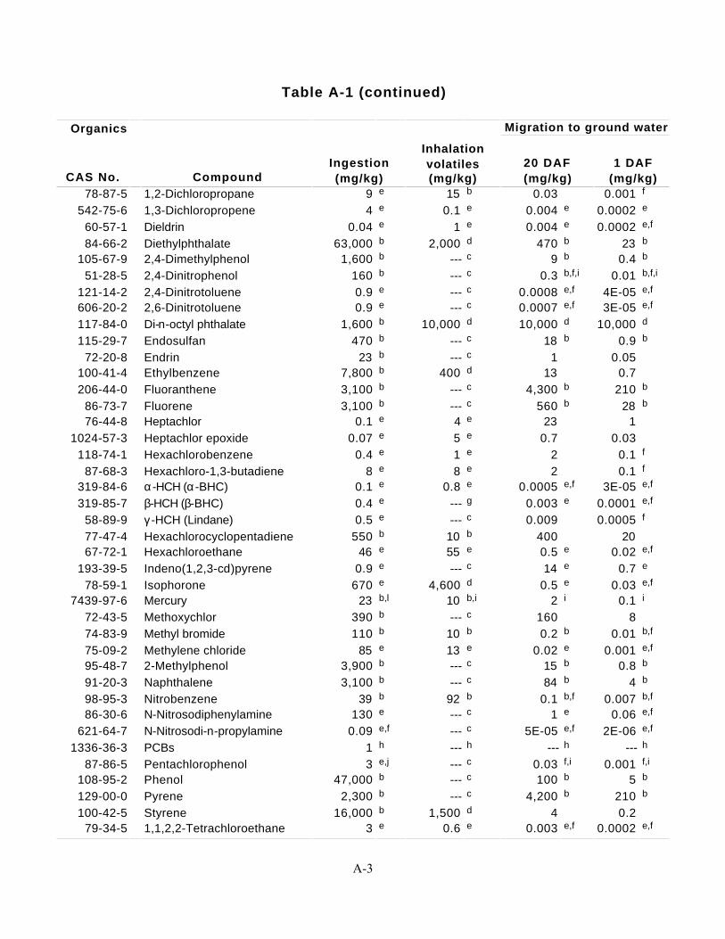
Table A-1 (continued)
Organics Migration to ground water
CAS No. CompoundIngestion(mg/kg)
Inhalationvolatiles(mg/kg)
20 DAF(mg/kg)
1 DAF(mg/kg)
78-87-5 1,2-Dichloropropane 9 e 15 b 0.03 0.001 f
542-75-6 1,3-Dichloropropene 4 e 0.1 e 0.004 e 0.0002 e
60-57-1 Dieldrin 0.04 e 1 e 0.004 e 0.0002 e,f
84-66-2 Diethylphthalate 63,000 b 2,000 d 470 b 23 b
105-67-9 2,4-Dimethylphenol 1,600 b --- c 9 b 0.4 b
51-28-5 2,4-Dinitrophenol 160 b --- c 0.3 b,f,i 0.01 b,f,i
121-14-2 2,4-Dinitrotoluene 0.9 e --- c 0.0008 e,f 4E-05 e,f
606-20-2 2,6-Dinitrotoluene 0.9 e --- c 0.0007 e,f 3E-05 e,f
117-84-0 Di-n-octyl phthalate 1,600 b 10,000 d 10,000 d 10,000 d
115-29-7 Endosulfan 470 b --- c 18 b 0.9 b
72-20-8 Endrin 23 b --- c 1 0.05100-41-4 Ethylbenzene 7,800 b 400 d 13 0.7206-44-0 Fluoranthene 3,100 b --- c 4,300 b 210 b
86-73-7 Fluorene 3,100 b --- c 560 b 28 b
76-44-8 Heptachlor 0.1 e 4 e 23 11024-57-3 Heptachlor epoxide 0.07 e 5 e 0.7 0.03
118-74-1 Hexachlorobenzene 0.4 e 1 e 2 0.1 f
87-68-3 Hexachloro-1,3-butadiene 8 e 8 e 2 0.1 f
319-84-6 α-HCH (α-BHC) 0.1 e 0.8 e 0.0005 e,f 3E-05 e,f
319-85-7 β-HCH (β-BHC) 0.4 e --- g 0.003 e 0.0001 e,f
58-89-9 γ -HCH (Lindane) 0.5 e --- c 0.009 0.0005 f
77-47-4 Hexachlorocyclopentadiene 550 b 10 b 400 2067-72-1 Hexachloroethane 46 e 55 e 0.5 e 0.02 e,f
193-39-5 Indeno(1,2,3-cd)pyrene 0.9 e --- c 14 e 0.7 e
78-59-1 Isophorone 670 e 4,600 d 0.5 e 0.03 e,f
7439-97-6 Mercury 23 b,l 10 b,i 2 i 0.1 i
72-43-5 Methoxychlor 390 b --- c 160 874-83-9 Methyl bromide 110 b 10 b 0.2 b 0.01 b,f
75-09-2 Methylene chloride 85 e 13 e 0.02 e 0.001 e,f
95-48-7 2-Methylphenol 3,900 b --- c 15 b 0.8 b
91-20-3 Naphthalene 3,100 b --- c 84 b 4 b
98-95-3 Nitrobenzene 39 b 92 b 0.1 b,f 0.007 b,f
86-30-6 N-Nitrosodiphenylamine 130 e --- c 1 e 0.06 e,f
621-64-7 N-Nitrosodi-n-propylamine 0.09 e,f --- c 5E-05 e,f 2E-06 e,f
1336-36-3 PCBs 1 h --- h --- h --- h
87-86-5 Pentachlorophenol 3 e,j --- c 0.03 f,i 0.001 f,i
108-95-2 Phenol 47,000 b --- c 100 b 5 b
129-00-0 Pyrene 2,300 b --- c 4,200 b 210 b
100-42-5 Styrene 16,000 b 1,500 d 4 0.279-34-5 1,1,2,2-Tetrachloroethane 3 e 0.6 e 0.003 e,f 0.0002 e,f
A-3
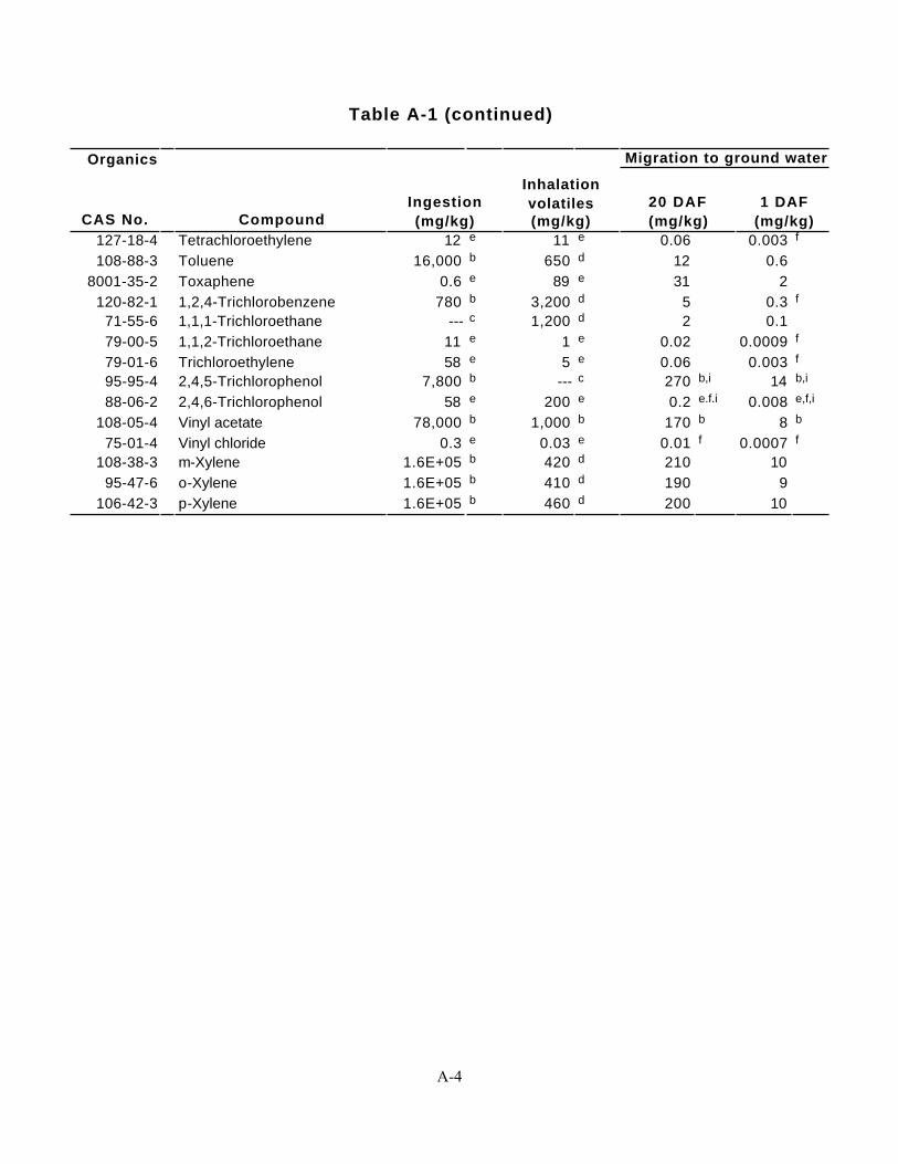
Table A-1 (continued)
Organics Migration to ground water
CAS No. CompoundIngestion(mg/kg)
Inhalationvolatiles(mg/kg)
20 DAF(mg/kg)
1 DAF(mg/kg)
127-18-4 Tetrachloroethylene 12 e 11 e 0.06 0.003 f
108-88-3 Toluene 16,000 b 650 d 12 0.68001-35-2 Toxaphene 0.6 e 89 e 31 2
120-82-1 1,2,4-Trichlorobenzene 780 b 3,200 d 5 0.3 f
71-55-6 1,1,1-Trichloroethane --- c 1,200 d 2 0.179-00-5 1,1,2-Trichloroethane 11 e 1 e 0.02 0.0009 f
79-01-6 Trichloroethylene 58 e 5 e 0.06 0.003 f
95-95-4 2,4,5-Trichlorophenol 7,800 b --- c 270 b,i 14 b,i
88-06-2 2,4,6-Trichlorophenol 58 e 200 e 0.2 e.f.i 0.008 e,f,i
108-05-4 Vinyl acetate 78,000 b 1,000 b 170 b 8 b
75-01-4 Vinyl chloride 0.3 e 0.03 e 0.01 f 0.0007 f
108-38-3 m-Xylene 1.6E+05 b 420 d 210 1095-47-6 o-Xylene 1.6E+05 b 410 d 190 9
106-42-3 p-Xylene 1.6E+05 b 460 d 200 10
A-4

Table A-1 (continued)
Inorganics Migration to ground water
CAS No. CompoundIngestion(mg/kg)
Inhalationfugitive
particulate(mg/kg)
20 DAF(mg/kg)
1 DAF(mg/kg)
7440-36-0 Antimony 31 b --- c 5 0.3
7440-38-2 Arsenic 0.4 e 750 e 29 i 1 i
7440-39-3 Barium 5,500 b 6.9E+05 b 1,600 i 82 i
7440-41-7 Beryllium 0.1 e 1,300 e 63 i 3 i
7440-43-9 Cadmium 78 b,m 1,800 e 8 i 0.4 i
7440-47-3 Chromium (total) 390 b 270 e 38 i 2 i
16065-83-1 Chromium (III) 78,000 b --- c --- g --- g
18540-29-9 Chromium (VI) 390 b 270 e 38 i 2 i
57-12-5 Cyanide (amenable) 1,600 b --- c 40 2
7439-92-1 Lead 400 k --- k --- k --- k
7440-02-0 Nickel 1,600 b 13,000 e 130 i 7 i
7782-49-2 Selenium 390 b --- c 5 i 0.3 i
7440-22-4 Silver 390 b --- c 34 b,i 2 b,i
7440-28-0 Thallium --- c --- c 0.7 i 0.04 i
7440-62-2 Vanadium 550 b --- c 6,000 b 300 b
7440-66-6 Zinc 23,000 b --- c 12,000 b,i 620 b,i
DAF = Dilution and attenuation factor.a Screening levels based on human health criteria only.b Calculated values correspond to a noncancer hazard quotient of 1.c No toxicity criteria available for that route of exposure.d Soil saturation concentration (Csat).e Calculated values correspond to a cancer risk level of 1 in 1,000,000.f Level is at or below Contract Laboratory Program required quantitation limit for Regular Analytical Services (RAS).g Chemical-specific properties are such that this pathway is not of concern at any soil contaminant concentration.h A preliminary remediation goal of 1 mg/kg has been set for PCBs based on Guidance on Remedial Actions for Superfund Sites
with PCB Contamination (U.S. EPA, 1990) and on EPA efforts to manage PCB contamination.i SSL for pH of 6.8.j Ingestion SSL adjusted by a factor of 0.5 to account for dermal exposure.k A screening level of 400 mg/kg has been set for lead based on Revised Interim Soil Lead Guidance for CERCLA Sites and
RCRA Corrective Action Facilities (U.S. EPA, 1994).l SSL is based on RfD for mercuric chloride (CAS No. 007487-94-7).m SSL is based on dietary RfD.
A-5

Table A-2. Generic SSLs: Default Parameters and Assumptions
Parameter
SSL pathway
DefaultInhalationMigration to
ground water
Source Characteristics
Continuous vegetative cover l 50 percentRoughness height m 0.5 cm for open terrain; used to derive Ut,7
Source area (A) l m 0.5 acres (2,024 m2); used to derive L forMTG
Source length (L) l 45 m (assumes square source)
Source depth m Extends to water table (i.e., no attenuationin unsaturated zone)
Soil Characteristics
Soil texture m m Loam; defines soil characteristics/parameters
Dry soil bulk density (ρb) l l 1.5 kg/L
Soil porosity (n) l m 0.43
Vol. soil water content (θw) l l 0.15 (INH); 0.30 (MTG)
Vol. soil air content (θa) l l 0.28 (INH); 0.13 (MTG)
Soil organic carbon (foc) l l 0.006 (0.6%, INH); 0.002 (0.2 %, MTG)
Soil pH m m 6.8; used to determine pH-specific Kd
(metals) and Koc (ionizable organics)
Mode soil aggregate size m 0.5 mm; used to derive Ut,7
Threshold windspeed @ 7 m (Ut,7) l 11.32 m/s
Meteorological Data
Mean annual windspeed (Um) l 4.69 m/s (Minneapolis, MN)
Air dispersion factor (Q/C) l 90th percentile conterminous U.S.
Volatilization Q/C l 68.81; Los Angeles, CA; 0.5-acre source
Fugitive particulate Q/C l 90.80; Minneapolis, MN; 0.5-acre source
Hydrogeologic CharacteristicsHydrogeologic setting m Generic (national); surficial aquifer
Dilution/attenuation factor (DAF) l 20
l Indicates input parameters directly used in SSL equations.m Indicates parameters/assumptions used to develop SSL input parameters.INH = Inhalation pathway.MTG = Migration to ground water pathway.
A-6

Analysis of Effects of Source Size on Generic SSLs
A large number of commenters on the December 1994 Soil Screening Guidance suggested that mostcontaminated soil sources were 0.5 acre or less. Before changing this default assumption from 30 acresto 0.5 acre, the Office of Emergency and Remedial Response (OERR) conducted an analysis of theeffects of changing the area of a contaminated soil source on generic SSLs calculated for the inhalationand migration to ground water exposure pathways. This analysis includes:
• An analysis of the sensitivity of SSLs to a change in source area from 30 acres to 0.5acre
• Mass-limit modeling results showing the depth of contamination for a 30-acre sourcethat corresponds to a 0.5-acre SSL.
All equations, assumptions, and model input parameters used in this analysis are consistent with thosedescribed in Part 2 of this document unless otherwise indicated. Chemical properties used in theanalysis are described in Part 5 of this document.
In summary, the results of this analysis indicate that:
• The SSLs are not particularly sensitive to varying the source area from 30 acres to 0.5acre. This reduction in source area lowers SSLs for the inhalation pathway by about afactor of 2 and lowers SSLs for the migration to ground water pathway by a factor of2.9 under typical hydrogeologic conditions.
• Half-acre SSLs calculated for 43 volatile and semivolatile contaminants using theinfinite source models correspond to mass-limit SSLs for a 30-acre source uniformlycontaminated to a depth of about 1 to 21 meters (depending on contaminant andpathway); the average depth is 8 meters for the inhalation pathway (21 contaminants)and 11 meters for the migration to ground water pathway (43 contaminants).
Sensitivity Analysis. For the inhalation pathway, source area affects the Q/C value (a measureof dispersion), which directly affects the final SSL and is not chemical-specific. Higher Q/C valuesresult in higher SSLs. As shown in Table 3 (Section 2.4.3), the effect of area on the Q/C value is notsensitive to meteorological conditions, with the ratio of a 0.5-acre Q/C to a 30-acre Q/C ranging from1.93 to 1.96 over the 29 conditions analyzed. Decreasing the source area from 30 acres to 0.5 acrewill therefore increase inhalation SSLs by about a factor of 2.
For the migration to ground water pathway, source area affects the DAF, which also directly affectsthe final SSLs and is not chemical-specific. The sensitivity analysis for the dilution factor is morecomplicated than for Q/C because increasing source area (expressed as the length of source parallel toground water flow) not only increases infiltration to the aquifer, which decreases the dilution factor,but also increases the mixing zone depth, which tends to increase the dilution factor. The first effectgenerally overrides the second (i.e., longer sources have lower dilution factors) except for very thickaquifers (see Section 2.5.7).
The sensitivity analysis described in Section 2.5.7 shows that the dilution model is most sensitive tothe aquifer's Darcy velocity (i.e., hydraulic conductivity H hydraulic gradient). For a less conservativeDarcy velocity (90th percentile), decreasing the source area from 30 acres to 0.5 acre increased thedilution factor by a factor of 3.1 (see Table 9, Section 2.5.7). For the conditions analyzed, decreasingthe source area from 30 acres to 0.5 acre affected dilution factor from no increase to a factor of 4.3increase. No increase in dilution factor for a 0.5-acre source was observed for the less conservative
A-7

(higher) aquifer thickness (46 m). In this case the decrease in mixing zone depth balances the decreasein infiltration rate for the smaller source.
Mass-Limit Analysis. The infinite source assumption is one of the more conservativeassumptions inherent in the SSL models, especially for small sources. This assumption should provideadequate protection for sources with larger areas than those used to calculate SSLs. To test thishypothesis the SSL mass-limit models (Section 2.6) were used to calculate, for 43 volatile andsemivolatile chemicals, the depth at which a mass-limit SSL for a 30-acre source is equal to a 0.5-acreinfinite-source SSL.
The mass-limit models are simple mass-balance models that calculate SSLs based on the conservativeassumption that the entire mass of contamination in a source either volatilizes (inhalation model) orleaches (migration to ground water model) over the exposure period of interest. These models weredeveloped to correct the mass-balance violation in the infinite source models for highly volatile orsoluble contaminants.
Table A-3 presents the results of this analysis. These results demonstrate that 0.5-acre infinite sourceSSLs are protective of uniformly contaminated 30-acre source areas of significant depth. For the 21chemicals analyzed for the inhalation pathway, these source depths range up to 21 meters, with anaverage depth of 8 meters and a standard deviation of 5.7. For the migration to ground water pathway,source depths for 43 contaminants range to 21 meters, with an average of 11 meters and a standarddeviation of 5.4.
References
U.S. EPA (Environmental Protection Agency). 1990. Guidance on Remedial Actions for SuperfundSites with PCB Contamination. Office of Solid Waste and Emergency Response, Washington,DC. NTIS PB91-921206CDH.
U.S. EPA (Environmental Protection Agency). 1994. Revised Interim Soil Lead Guidance forCERCLA Sites and RCRA Corrective Action Facilities. Office of Solid Waste and EmergencyResponse, Washington, DC. Directive 9355.4-12.
A-8

Table A-3.Source Depth where 30-acrea Mass-Limit SSLs = 0.5-acreb
Infinite-Source SSLsc
Source depth (m)
Chemical Inhalation Migration to ground waterc
Acetone NA 21 Benzene 8.1 12 Benzoic acid NA 21 Bis(2-chloroethyl)ether 0.7 18 Bromodichloromethane NA 13
Bromoform 0.9 11Butanol NA 20 Carbon disulfide 19 11 Carbon tetrachloride 11 6 Chlorobenzene 3.5 6 Chlorodibromomethane NA 13
Chloroform 8.3 14 2-Chlorophenol NA 4 1,2-Dichlorobenzene NA 3 1,4-Dichlorobenzene NA 3 1,1-Dichloroethane 9.1 15 1,2-Dichloroethane 5.6 18
1,1-Dichloroethylene 15 10 cis-1,2-Dichloroethylene NA 15 trans-1,2-Dichloroethylene NA 12 2,4-Dichlorophenol NA 8 1,2-Dichloropropane 6.2 14 1,3-Dichloropropene 12 12 2,4-Dimethylphenol NA 7
2,4-Dinitrophenol NA 21 2,4-Dinitrotoluene NA 11 2,6-Dinitrotoluene NA 12 Ethylbenzene NA 4 Methyl bromide 12 17 Methylene chloride 8.9 18
2-Methylphenol NA 11 Nitrobenzene 0.5 13 1,1,2,2-Tetrachloroethane 1.6 11 Tetrachloroethylene 8.7 7 Toluene NA 7 1,1,1-Trichloroethane NA 9
1,1,2-Trichloroethane 3.4 14 Trichloroethylene 6.8 7 Vinyl acetate 4.6 20
A-9

Table A-3. (continued)
Source depth (m)
Chemical Inhalation Migration to ground waterc
Vinyl chloride 21 13 m-Xylene NA 4 o-Xylene NA 4 p-Xylene NA 4
NA = Risk-based SSL not available.a Q/C = 35.15; DAF = 10.b Q/C = 68.81; DAF = 20.c Migration to ground water mass-limit analysis based on 70-yr exposure duration and 0.18 m/yr infiltration rate.
A-10

APPENDIX B
Route-to-Route Extrapolation of InhalationBenchmarks

APPENDIX B
Route-to-Route Extrapolation of Inhalation Benchmarks
Introduction
For a number of the contaminants commonly found at Superfund sites, inhalation benchmarks fortoxicity are not available from IRIS or HEAST. As pointed out by commenters to the December1994 Soil Screening Guidance , ingestion SSLs tend to be higher than inhalation SSLs for mostvolatile chemicals with both inhalation and ingestion benchmarks. This suggests that ingestion SSLsmay not be adequately protective for inhalation exposure to chemicals that lack inhalationbenchmarks.
To address this concern, the Office of Emergency and Remedial Response (OERR) evaluatedpotential approaches for deriving inhalation benchmarks using route-to-route extrapolation fromoral benchmarks (e.g., inhalation reference concentrations [RfCs] from oral reference doses [RfDs]).OERR evaluated Agency initiatives concerning route-to-route extrapolation, including: the potentialreactivity of airborne toxicants (e.g., portal-of-entry effects), the pharmacokinetic behavior oftoxicants for different routes of exposure (e.g., absorption by the gut versus absorption by the lung),and the significance of physicochemical properties in determining dose (e.g., volatility, speciation).During this process, OERR consulted with staff in the EPA Office of Research and Development(ORD) to identify appropriate techniques and key technical aspects in performing route-to-routeextrapolation. The following sections describe OERR’s analysis of route-to-route extrapolation andthe conclusions reached regarding the use of extrapolated inhalation benchmarks to supportinhalation SSLs.
B.1 Extrapolation of Inhalation Benchmarks
The first step taken in considering route-to-route extrapolation of inhalation benchmarks was tocompare existing inhalation benchmarks to inhalation benchmarks extrapolated from oral studies.This comparison was important to determine whether a simple route-to-route extrapolation couldprovide a defensible inhalation benchmark for chemicals lacking appropriate inhalation studies.OERR identified nine chemicals found in IRIS (Integrated Risk Information System) that haveverified RfDs and RfCs for noncancer effects, including three chemicals found in the SSL guidance(ethylbenzene, styrene, and toluene). Reference concentrations for inhalation exposure wereextrapolated from oral reference doses for adults using the following formula:
extrapolated RfC á mg / m 3 é = RfD á mg / kg − d é H 70 kg
20 m 3 / d (B-1)
.
It is important to note that dosimetric adjustments were not made to account for respiratory tractdeposition efficiency and distribution; physical, biological, and chemical factors; and other aspects ofexposure (e.g., discontinuous exposure) that affect uptake and clearance. Consequently, this simpleextrapolation method relies on the implicit assumption that the route of administration is irrelevantto the dose delivered to a target organ, an assumption not supported by the principles of dosimetryor pharmacokinetics.
B-1

The limited data on noncarcinogens suggest that more volatile constituents tend to haveextrapolated RfCs closer to the RfCs developed by EPA (i.e., extrapolated RfC within a factor of 3of the RfC in IRIS). The less volatile chemicals (e.g., dichlorvos) tend to be below the RfCsdeveloped by EPA workgroups by 1 to 3 orders of magnitude. Although this data set is insufficient todiscern trends in extrapolated versus IRIS RfCs, two points are reasonably clear: (1) for some volatilechemicals, route-to-route extrapolation results in inhalation benchmarks reasonably close to the RfC,and (2) as volatility decreases and/or chemical speciation becomes important (e.g., hydrogen sulfide)with respect to environmental chemistry and toxicology, the uncertainty in extrapolated inhalationbenchmarks is likely to increase.
For carcinogens, OERR identified 41 chemicals in IRIS for which oral cancer slope factors (CSForal)and inhalation unit risk factors (URFs) are available, including 23 chemicals covered under the SSLguidance. Unit risk factors for inhalation exposure were extrapolated from oral carcinogenic slopefactors for adults using the following formula:
URF ( µ g / m 3 ) − 1 = CSForal ( mg / kg − d ) − 1
70 kg H 20 m 3 / d H 10− 3 mg / µ g
(B-2) .
Using the extrapolated URF, risk-specific air concentrations were calculated as a lifetime averageexposure concentration as shown in equation B-3:
extrapolated air concentration µg / m3 = target risk 10−6
URF (µg / m3 )−1
(B-3) .
Not surprisingly, the risk-based (i.e., 10-6) air concentrations in IRIS are the same as the airconcentrations extrapolated from the CSForal for 30 of the 41 carcinogenic chemicals evaluated (atone significant figure). Historically, oral and inhalation slope factors have been based on oral studiesfor chemicals for which pharmacokinetic or portal-of-entry effects were considered insignificant. Asa result, route of exposure extrapolations were often included in the development of the carcinogenicslope factors. However, the divergence of extrapolated air concentrations with risk-based (i.e., 10 -6)air concentrations in IRIS reflects newer methods in use at EPA that address portal-of-entry effects,dosimetry, and pharmacokinetic behavior. For example, 1,2-dibromomethane has an extrapolated10-6 air concentration that is 2 orders of magnitude below the value in IRIS. This difference isprobably attributable to differences in: (1) the endpoint for inhalation exposure (nasal cavitycarcinoma) versus oral exposure (squamous cell carcinoma), and/or (2) portal-of-entry effectsdirectly related to deposition physiology and absorption of 1,2-dibromomethane.
B.2 Comparison of Extrapolated Inhalation SSLs with Generic SSLs
Having performed a simple extrapolation of inhalation benchmarks, the next step was to comparethe inhalation SSLs (SSLinh) based on extrapolated data to the soil saturation concentrations* (Csat)and generic SSLs for soil ingestion (SSLing) and ground water ingestion (SSLgw). Table B-1 presentsthe 50 organic chemicals in the SSL guidance that lack inhalation benchmarks. The table presentsoral benchmarks found in IRIS (columns 2 and 3) and extrapolated inhalation benchmarks as
* The derivation of Csat and its significance is discussed in Section 2.4.4 of this Technical Background Document.
B-2

described in Equations B-1 and B-2 (columns 4 and 5). In addition, the table presents volatilization-based SSLs and SSLs based on particulate emissions derived from the extrapolated toxicity values. Foreach column of extrapolated inhalation SSLs in this table, values are truncated at 1,000,000 mg/kgbecause the soil concentration cannot be greater than 100 percent (i.e., 1,000,000 ppm).
B.2.1 Comparison of Extrapolated SSLs Based on Volatilization
The extrapolated SSLinh for volatilization (SSLinh-v) was calculated with Equation 4 in Section 2.4using a chemical-specific volatilization factor (VF). In Table B-1, the SSLinh-v values based onextrapolated inhalation benchmarks (column 6) are compared with the soil saturation concentration(Csat, column 7) and generic migration to ground water SSLs assuming a dilution attenuation factor(DAF) of 20 (SSLgw).
As described in Section 2.4.4, Csat represents the concentration at which soil pore air is saturated witha chemical and maximum volatile emissions are reached. A comparison of the Csat with theextrapolated SSLinh-v values indicates that, for 36 of the 50 contaminants, SSLinh-v exceeds the soilsaturation concentration, often by several orders of magnitude. Because maximum volatile emissionsoccur at Csat, these 36 contaminants are not likely to pose significant risks through the inhalationpathway, and therefore the lack of inhalation benchmarks is not likely to underestimate risk throughthe volatilization pathway.
For the remaining 14 contaminants with extrapolated SSLinh-v values below Csat, all are above thegeneric SSLgw values. This analysis suggests that SSLs based on the migration-to-groundwater pathwayare likely to be protective of the inhalation pathway as well. However, for sites where groundwater isnot of concern, the SSLs based on ingestion may not necessarily be protective of the inhalationpathway. The analysis indicates that the extrapolated inhalation SSLs are below SSLs based on directingestion for the following chemicals: acetone, bromodichloromethane, chlorodibromomethane, cis-1,2-dichloroethylene, and trans-1,2-dichloroethylene. This analysis supports the possibility thatthe SSLs based on direct ingestion for the listed chemicals may not be adequately protective ofinhalation exposures. However, a more rigorous evaluation of the route-to-route extrapolationmethods used to derive the toxicity criteria for this analysis is warranted (refer to section B.3).
B.2.2 Comparison of Extrapolated SSLs Based on Particulate Emissions
The extrapolated particulate inhalation SSLs (SSLinh-p) were calculated with Equation 4 in Section 2.4using the particulate emission factor (PEF) of 1.32 x 10⁹ m3/kg. Table B-1 compares the SSLinh-p
values based on extrapolated benchmarks (column 10) and generic SSLs based on direct ingestion(SSLing, Column 9). This comparison indicates that the extrapolated SSLinh-p values that are based onthe PEF are well above the SSLs for soil ingestion. Thus, ingestion SSLs are likely to be protective ofinhalation risks from fugitive dusts from surface soils.
B.3 Conclusions and Recommendations
Based on the results presented in this appendix, OERR reached several conclusions regarding route-to-route extrapolation of inhalation benchmarks for the development of generic inhalation SSLs.First, it is reasonable to assume that, for some contaminants, the lack of inhalation benchmarks mayunderestimate risks due to inhalation exposure. Of the 17 volatile organics for which both theingestion and inhalation SSLs are based on IRIS benchmarks, all had inhalation SSLs that were belowthe ingestion SSLs. Nevertheless, generic SSLs for ground water ingestion (DAF of 20) are lower,
B-3
often significantly lower, than both extrapolated and IRIS-based inhalation SSLs with the exceptionof vinyl chloride, which is gaseous at ambient temperatures. Thus, at sites where ground water is ofconcern, migration to ground water SSLs generally will be protective from the standpoint ofinhalation risk. However, if the ground water is not of concern at a site (e.g., if ground water belowthe site is not potable), the use of SSLs for soil ingestion may not be adequately protective of theinhalation pathway.
Second, the extrapolated SSLinh values are not intended to be used as generic SSLs for siteinvestigations; the extrapolated inhalation SSLs are useful in determining the potential forinhalation risks but should not be misused as SSLs. Route-to-route extrapolation methods mustaccount for the relationship between physicochemical properties and absorption and distribution oftoxicants, the significance of portal-of-entry effects, and the potential differences in metabolicpathways associated with the intensity and duration of inhalation exposure. However, methodsrequired to generate sufficiently rigorous inhalation benchmarks have recently been developed by theORD. A final guidance document was made available by ORD in November of 1995 that addressesmany of the issues critical to the development of inhalation benchmarks described above. Thedocument, entitled Methods for Derivation of Inhalation Reference Concentrations and Applicationof Inhalation Dosimetry (U.S. EPA, 1994), describes the application of inhalation dosimetry toderive inhalation reference concentrations and represents the current state-of-the-science at EPAwith respect to inhalation benchmark development. The fundamentals of inhalation dosimetry arepresented with respect to toxicokinetics and the physicochemical properties of chemicalcontaminants.
Thus, at sites where the migration to ground water pathway is not of concern and a site managerdetermines that the inhalation pathway may be significant for contaminants lacking inhalationbenchmarks, route-to-route extrapolation may be performed using EPA-approved methods on acase-by-case basis. Chemical-specific route-to-route extrapolations should be accompanied by acomplete discussion of the data, underlying assumptions, and uncertainties identified in theextrapolation process. Extrapolation methods should be consistent with the EPA guidance presentedin Methods for Derivation of Inhalation Reference Concentrations and Application of InhalationDosimetry. If a route-to-route extrapolation is found not to be appropriate based on the ORDguidance, the information on extrapolated SSLs may be included as part of the uncertainty analysis ofthe baseline risk assessment for the site.
Reference
U.S. EPA (Environmental Protection Agency). 1994. Methods for Derivation of InhalationReference Concentrations and Application of Inhalation Dosimetry. EPA/600/8-90/066F.Office of Research and Development, Washington, DC.
B-4

Tab
le B
-1.
Co
mp
aris
on
of
Co
mp
ou
nd
Ace
naph
then
e
Ace
ton
eA
nthr
acen
e
Ben
z(a)
anth
race
ne
Ben
zo(b
)flu
oran
then
e
Ben
zo(k
)flu
oran
then
e
Ben
zo(a
)py
rene
Ben
zoic
aci
d
Bis
(2-e
thyl
hexy
l)pht
hala
te
Bro
mo
dic
hlo
rom
eth
ane
But
anol
But
yl b
enzy
l pht
hala
teC
arba
zole
p-C
hlor
oani
line
Ch
loro
dib
rom
om
eth
ane
2-C
hlor
ophe
nol
Chr
ysen
e
DD
D
DD
E
Dib
enz(
a,h)
anth
race
ne
Di-n
-but
yl p
htha
late
3,3'
-Dic
hlor
oben
zidi
ne,
cis
-1,2
-Dic
hlo
roet
hyl
ene
tran
s-1
,2-D
ich
loro
eth
ylen
e2,
4-D
ichl
orop
heno
l
Die
thyl
phth
alat
e
2,4-
Dim
ethy
lphe
nol
2,4-
Din
itrop
heno
l
2,4-
Din
itrot
olue
ne
2,6-
Din
itrot
olue
ne
Di-n
-oct
yl p
htha
late
End
osul
fan
End
rin
Flu
oran
then
e
Ext
rap
ola
ted
Inh
alat
ion
SS
Ls
(SS
Lin
h)
wit
h S
oil
Co
nce
ntr
atio
ns
(Csa
t), a
nd
Mig
rati
on
to
Gro
un
d W
ater
(S
SL
gw)
IRIS
ora
l ben
chm
arks
Ext
rap
ola
ted
inh
alat
ion
b
ench
mar
ksV
F-b
ased
SS
Ls
(mg
/kg
)P
EF
-bas
ed S
SL
s (m
g/k
g)
RfD
(mg
/kg
-d)-
CS
F
(mg
/kg
-d)-1
RfC
(mg
/m3 )
UR
F
(mg
/m3 )
-1
Ext
rap
ola
ted
vo
lati
lizat
ion
S
SL
inh
-vC
sat
Gen
eric
SS
Lg
w
(DA
F 2
0)G
ener
ic
SS
Lin
g
Ext
rap
ola
ted
p
arti
cula
te S
SL
inh
-p
6E-0
22.
1E-0
1
48,0
0018
157
04,
700
>1,
000,
000
1E-0
13.
5E-0
1
4,60
010
3,74
716
7,80
0>
1,00
0,00
03E
-01
1.1E
+00
86
0,00
08
12,0
0023
,000
>1,
000,
000
7.3
E-0
1
2.1E
-04
110
222
0.9
15,0
007.
3 E
-01
2.
1E-0
454
115
0.9
15,0
007.
3 E
-02
2.
1E-0
54,
600
649
915
0,00
07.
3 E
+00
2.
1E-0
328
108
0.09
1,50
04E
+00
1.4E
+01
>
1,00
0,00
036
340
031
0,00
0>
1,00
0,00
01.
4 E
-02
4.
0E-0
613
0,00
030
,804
3,60
046
800,
000
6.2
E-0
2
1.8E
-05
1.14
2,98
10.
610
180,
000
1E-0
13.
5E-0
1
14,0
0010
,477
177,
800
>1,
000,
000
2E-0
17.
0E-0
1
>1,
000,
000
928
930
16,0
00>
1,00
0,00
02.
0 E
-02
5.
7E-0
61,
100
153
0.6
3256
0,00
04E
-03
1.4E
-02
4,10
02,
632
0.7
310
>1,
000,
000
8.4
E-0
2
2.4E
-05
1.5
1,26
00.
48
130,
000
5E-0
31.
8E-0
2
550
53,4
824
390
>1,
000,
000
7.3
E-0
3
2.1E
-06
3,20
04
160
88>
1,00
0,00
02.
4 E
-01
6.
9E-0
582
054
016
347
,000
3.4
E-0
1
9.7E
-05
620
3,21
854
233
,000
7.3
E+
00
2.1E
-03
120
572
0.09
1,50
01E
-01
3.5E
-01
>
1,00
0,00
02,
279
2,30
07,
800
>1,
000,
000
4.5
E-0
1
1.3E
-04
2414
01
25,0
001E
-02
3.5E
-02
11
01,
205
0.4
780
>1,
000,
000
2E-0
27.
0E-0
2
170
3,06
70.
71,
600
>1,
000,
000
3E-0
31.
1E-0
2
2,50
04,
419
124
0>
1,00
0,00
08E
-01
2.8E
+00
>
1,00
0,00
01,
974
470
63,0
00>
1,00
0,00
02E
-02
7.0E
-02
19
,000
10,6
569
1,60
0>
1,00
0,00
02E
-03
7.0E
-03
1,
000
279
0.3
160
>1,
000,
000
6.8E
-01
1.9E
-04
418
20.
0008
0.9
17,0
006.
8E-0
11.
9E-0
44
940.
0007
0.9
17,0
002E
-02
7.0E
-02
>
1,00
0,00
09,
984
10,0
001,
600
>1,
000,
000
6E-0
32.
1E-0
2
18,0
007
1847
0>
1,00
0,00
03E
-04
1.1E
-03
2,
500
181
23>
1,00
0,00
04E
-02
1.4E
-01
45
0,00
013
243
003,
100
>1,
000,
000
B-5

Tab
le B
-1.
Co
mp
aris
on
of
Co
mp
ou
nd
Flu
oren
e
γ-H
exac
hlor
ocyc
lohe
xane
Inde
no(
1,2,
3-cd
)py
rene
Isop
horo
neM
etho
xych
lor
2-M
ethy
lphe
nol
Nap
htha
lene
N-N
itros
odip
heny
lam
ine
N-N
itros
odi-n
-pro
pyla
min
eP
enta
chlo
roph
enol
Phe
nol
Pyr
ene
2,4,
5-T
richl
orop
heno
l
m-X
ylen
e
o-X
ylen
e
p-X
ylen
e
NR
= S
SL i
nh-v is
gre
ater
than
1,0
00,0
00 p
Bo
ld in
dic
ates
wh
ere
extr
apo
late
d S
SExt
rap
ola
ted
Inh
alat
ion
SS
Ls
(SS
Lin
h)
wit
h S
oil
Co
nce
ntr
atio
ns
(Csa
t), a
nd
Mig
rati
on
to
Gro
un
d W
ater
(S
SL
gw)
IRIS
ora
l ben
chm
arks
Ext
rap
ola
ted
inh
alat
ion
b
ench
mar
ksV
F-b
ased
SS
Ls
(mg
/kg
)P
EF
-bas
ed S
SL
s (m
g/k
g)
RfD
(mg
/kg
-d)-
CS
F
(mg
/kg
-d)-1
RfC
(mg
/m3 )
UR
F
(mg
/m3 )
-1
Ext
rap
ola
ted
vo
lati
lizat
ion
S
SL
inh
-vC
sat
Gen
eric
SS
Lg
w
(DA
F 2
0)G
ener
ic
SS
Lin
g
Ext
rap
ola
ted
p
arti
cula
te S
SL
inh
-p
4E-0
21.
4E-0
1
75,0
0016
456
03,
100
>1,
000,
000
1.3
E+
00
3.7E
-04
3.1
440.
009
0.5
8,60
07.
3 E
-01
2.
1E-0
466
00.
514
0.9
15,0
009.
5 E
-04
2.
7E-0
772
04,
570
0.5
670
>1,
000,
000
5E-0
31.
8E-0
2
74,0
0026
160
390
>1,
000,
000
5E-0
21.
8E-0
1
37,0
0016
,827
153,
900
>1,
000,
000
4E-0
21.
4E-0
1
8,20
037
584
3,10
0>
1,00
0,00
04.
9 E
-03
1.
4E-0
61,
000
275
113
0>
1,00
0,00
07.
0 E
+00
2.
0E-0
30.
12,
413
0.00
005
0.09
1,60
01.
2 E
-01
3.
4E-0
583
7,12
10.
033
94,0
006E
-01
2.1E
+00
40
0,00
022
,588
100
47,0
00>
1,00
0,00
03E
-02
1.1E
-01
42
0,00
085
4,20
02,
300
>1,
000,
000
1E-0
13.
5E-0
1
250,
000
11,6
1827
07,
800
>1,
000,
000
2E+
007.
0E+
00
45,0
0041
821
016
0,00
0>
1,00
0,00
02E
+00
7.0E
+00
45
,000
413
190
160,
000
>1,
000,
000
2E+
007.
0E+
00
41,0
0046
120
016
0,00
0>
1,00
0,00
0
ppm
(=
no
vola
tile
inha
latio
n ris
k at
any
soi
l con
cent
ratio
n)
SS
Lin
h v
alu
es a
re le
ss t
han
SS
L v
alu
es b
ased
on
dir
ect
ing
esti
on
.
B-6
1
APPENDIX C
Limited Validation of the Jury InfiniteSource and Jury
Finite Source Models (EQ, 1995)

2
LIMITED VALIDATION OF THE JURYINFINITE SOURCE AND JURY REDUCED
SOLUTION FINITE SOURCE MODELS FOREMISSIONS OF SOIL-INCORPORATED
VOLATILE ORGANIC COMPOUNDS
by
Environmental Quality Management, Inc.Cedar Terrace Office Park, Suite 250
3325 Chapel Hill BoulevardDurham, North Carolina 27707
Contract No. 68-D30035Work Assignment No. 1-55
Subcontract No. 95.5PN 5099-4
Janine Dinan, Work Assignment Manager
U.S. ENVIRONMENTAL PROTECTION AGENCYOFFICE OF SOLID WASTE AND EMERGENCY RESPONSE
WASHINGTON, D.C. 20460
July 1995

3
DISCLAIMER
This project has been performed under contract to E.H. Pechan & Associates, Inc. It wasfunded with Federal funds from the U.S. Environmental Protection Agency under Contract No.68-D30035. The content of this publication does not necessarily reflect the views or policies of theU.S. Environmental Protection Agency nor does mention of trade names, commercial products, ororganizations imply endorsement by the U.S. Government.

4
CONTENTS
Figures .. . . . . . . . . . . . . . . . . . . . . . . . . . . . . . . . . . . . . . . . . . . . . . . . . . . . . . . . . . . . . . . . . . . . . . . . . . . . . . . . . . . . . . . . . . . . . . . . . . . . ivTables .. . . . . . . . . . . . . . . . . . . . . . . . . . . . . . . . . . . . . . . . . . . . . . . . . . . . . . . . . . . . . . . . . . . . . . . . . . . . . . . . . . . . . . . . . . . . . . . . . . . .viAcknowledgment .. . . . . . . . . . . . . . . . . . . . . . . . . . . . . . . . . . . . . . . . . . . . . . . . . . . . . . . . . . . . . . . . . . . . . . . . . . . . . . . . . . . . . . . . . . . vii
1 . Introduction . . . . . . . . . . . . . . . . . . . . . . . . . . . . . . . . . . . . . . . . . . . . . . . . . . . . . . . . . . . . . . . . . . . . . . .C-1
Project objectives.. . . . . . . . . . . . . . . . . . . . . . . . . . . . . . . . . . . . . . . . . . . . . . . . . . . . . . . . . . . . . . . . . . . . . . . . . . . . . . . . . . . . . .C-2Technical approach.. . . . . . . . . . . . . . . . . . . . . . . . . . . . . . . . . . . . . . . . . . . . . . . . . . . . . . . . . . . . . . . . . . . . . . . . . . . . . . . . . . . .C-2
2 . Review of the Jury Volatilization Models. . . . . . . . . . . . . . . . . . . . . . . . . . . . . . . . . . . . . . .C-3
Finite source model derivation.. . .. . . . . . . . . . . . . . . . . . . . . . . . . . . . . . . . . . . . . . . . . . . . . . . . . . . . . . . . . . . . . . . . . . . .C-4Infinite source model derivation .. . . . . . . . . . . . . . . . . . . . . . . . . . . . . . . . . . . . . . . . . . . . . . . . . . . . . . . . . . . . . . . . . . . . .C-6Summary of model assumptions and limitations .. . . . . . . . . . . . . . . . . . . . . . . . . . . . . . . . . . . . . . . . . . . . . . . . . .C-7
3 . Model Validation . . . . . . . . . . . . . . . . . . . . . . . . . . . . . . . . . . . . . . . . . . . . . . . . . . . . . . . . . . . . . . . . . .C-9
Validation of the Jury Infinite Source Model. . . . . . . . . . . . . . . . . . . . . . . . . . . . . . . . . . . . . . . . . . . . . . . . . . . . . . . .C-9Validation of the Jury Reduced Solution Finite Source Model. . . . . . . . . . . . . . . . . . . . . . . . . . . . . . . . . . C-31
4 . Parametric Analysis of the Jury Volatilization Models . . . . . . . . . . . . . . . . . . . . . . C-35
Affects of soil parameters .. . . . . . . . . . . . . . . . . . . . . . . . . . . . . . . . . . . . . . . . . . . . . . . . . . . . . . . . . . . . . . . . . . . . . . . . . . C-35Affects of nonsoil parameters.. . . . . . . . . . . . . . . . . . . . . . . . . . . . . . . . . . . . . . . . . . . . . . . . . . . . . . . . . . . . . . . . . . . . . . C-36
5 . Conclusions . . . . . . . . . . . . . . . . . . . . . . . . . . . . . . . . . . . . . . . . . . . . . . . . . . . . . . . . . . . . . . . . . . . . . C-38
References .. . . . . . . . . . . . . . . . . . . . . . . . . . . . . . . . . . . . . . . . . . . . . . . . . . . . . . . . . . . . . . . . . . . . . . . . . . . . . . . . . . . . . . . . . . . . . . . . C-40
APPENDICES
A. Validation Data for the Jury Infinite Source Model. . . . . . . . . . . . . . . . . . . . . . . . . . . . . . . . . . . . . . . . . . . . . . . C-43B. Validation Data for the Jury Reduced Solution Finite Source Model. . . . . . . . . . . . . . . . . . . . . . . . . . . C-58
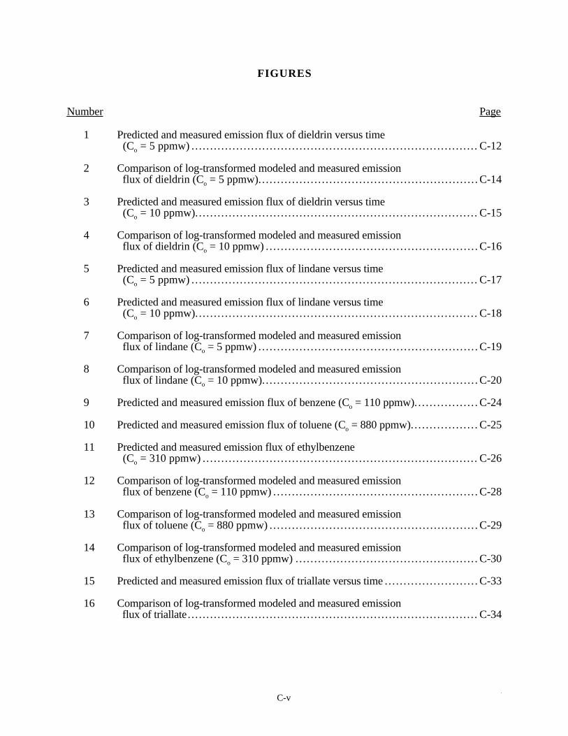
C-vv
FIGURES
Number Page
1 Predicted and measured emission flux of dieldrin versus time (Co = 5 ppmw) ... . . . . . . . . . . . . . . . . . . . . . . . . . . . . . . . . . . . . . . . . . . . . . . . . . . . . . . . . . . . . . . . . . . . . . . . . . . C-12
2 Comparison of log-transformed modeled and measured emission flux of dieldrin (Co = 5 ppmw).. . . . . . . . . . . . . . . . . . . . . . . . . . . . . . . . . . . . . . . . . . . . . . . . . . . . . . . . . . C-14
3 Predicted and measured emission flux of dieldrin versus time (Co = 10 ppmw)... . . . . . . . . . . . . . . . . . . . . . . . . . . . . . . . . . . . . . . . . . . . . . . . . . . . . . . . . . . . . . . . . . . . . . . . . . C-15
4 Comparison of log-transformed modeled and measured emission flux of dieldrin (Co = 10 ppmw) .. . . . . . . . . . . . . . . . . . . . . . . . . . . . . . . . . . . . . . . . . . . . . . . . . . . . . . . . C-16
5 Predicted and measured emission flux of lindane versus time (Co = 5 ppmw) ... . . . . . . . . . . . . . . . . . . . . . . . . . . . . . . . . . . . . . . . . . . . . . . . . . . . . . . . . . . . . . . . . . . . . . . . . . . C-17
6 Predicted and measured emission flux of lindane versus time (Co = 10 ppmw)... . . . . . . . . . . . . . . . . . . . . . . . . . . . . . . . . . . . . . . . . . . . . . . . . . . . . . . . . . . . . . . . . . . . . . . . . . C-18
7 Comparison of log-transformed modeled and measured emission flux of lindane (Co = 5 ppmw) .. . . . . . . . . . . . . . . . . . . . . . . . . . . . . . . . . . . . . . . . . . . . . . . . . . . . . . . . . . C-19
8 Comparison of log-transformed modeled and measured emission flux of lindane (Co = 10 ppmw).. . . . . . . . . . . . . . . . . . . . . . . . . . . . . . . . . . . . . . . . . . . . . . . . . . . . . . . . . C-20
9 Predicted and measured emission flux of benzene (Co = 110 ppmw).. . . . . . . . . . . . . . . . C-24
10 Predicted and measured emission flux of toluene (Co = 880 ppmw).. . . . . . . . . . . . . . . . . C-25
11 Predicted and measured emission flux of ethylbenzene (Co = 310 ppmw) ... . . . . . . . . . . . . . . . . . . . . . . . . . . . . . . . . . . . . . . . . . . . . . . . . . . . . . . . . . . . . . . . . . . . . . . . C-26
12 Comparison of log-transformed modeled and measured emission flux of benzene (Co = 110 ppmw) .. . . . . . . . . . . . . . . . . . . . . . . . . . . . . . . . . . . . . . . . . . . . . . . . . . . . . . C-28
13 Comparison of log-transformed modeled and measured emission flux of toluene (Co = 880 ppmw) .. . . . . . . . . . . . . . . . . . . . . . . . . . . . . . . . . . . . . . . . . . . . . . . . . . . . . . . C-29
14 Comparison of log-transformed modeled and measured emission flux of ethylbenzene (Co = 310 ppmw) .. . . . . . . . . . . . . . . . . . . . . . . . . . . . . . . . . . . . . . . . . . . . . . . . C-30
15 Predicted and measured emission flux of triallate versus time .. . . . . . . . . . . . . . . . . . . . . . . . C-33
16 Comparison of log-transformed modeled and measured emission flux of triallate.. . . . . . . . . . . . . . . . . . . . . . . . . . . . . . . . . . . . . . . . . . . . . . . . . . . . . . . . . . . . . . . . . . . . . . . . . . . . . C-34

C-vivi
TABLES
Number Page
1 Volatilization Model Input Values for Lindane and Dieldrin .. . . . . . . . . . . . . . . . . . . . . . . . . . C-11
2 Summary of the Bench-Scale Validation of the Jury Infinite Source Model.. . . . . . . . . . . . . . . . . . . . . . . . . . . . . . . . . . . . . . . . . . . . . . . . . . . . . . . . . . . . . . . . . . . . . . . . . . . . . . C-21
3 Volatilization Model Input Variables for Benzene, Toluene, and Ethylbenzene .. . . . . . . . . . . . . . . . . . . . . . . . . . . . . . . . . . . . . . . . . . . . . . . . . . . . . . . . . . . . . . . . . . . . . . . . . C-23
4 Summary of Statistical Analysis of Pilot-Scale Validation .. . . . . . . . . . . . . . . . . . . . . . . . . . . . C-27
5 Volatilization Model Input Values for Triallate.. . . . . . . . . . . . . . . . . . . . . . . . . . . . . . . . . . . . . . . . . . C-32

C-viivii
ACKNOWLEDGMENT
This report was prepared for the U.S. Environmental Protection Agency by EnvironmentalQuality Management, Inc. of Durham, North Carolina under contract to E.H. Pechan &Associates, Inc. Ms. Annette Najjar with E.H. Pechan & Associates, Inc. served as the projecttechnical monitor and Craig Mann with Environmental Quality Management, Inc. managed theproject and was author of the report. Janine Dinan of the U.S. Environmental Protection Agency'sToxics Integration Branch provided overall project direction and served as the Work AssignmentManager.

C-11
SECTION 1
INTRODUCTION
In December 1995, the U.S. Environmental Protection Agency (EPA) Office of SolidWaste and Emergency Response published the Draft Technical Background Document (TBD) forSoil Screening Guidance (U.S. EPA, 1994). This document provides the technical backgroundbehind the development of the Soil Screening Guidance for Superfund, and defines the SoilScreening Framework. The framework consists of a suite of methodologies for developing SoilScreening Levels (SSLs) for 107 chemicals commonly found at Superfund sites. An SSL isdefined as "a chemical concentration in soil below which there is no concern under theComprehensive Environmental Response Compensation and Liability Act (CERCLA) foringestion, inhalation, and migration to ground water exposure pathways...." (U.S. EPA, 1994).
The SSL inhalation pathway considers exposure to vapor-phase contaminants emitted fromsoils. Inhalation pathway SSLs are calculated using air pathway fate and transport models.Currently, the models and assumptions used to calculate SSLs for inhalation of volatiles areupdates of risk assessment methods presented in the Risk Assessment Guidance for Superfund(RAGS) Part B (U.S. EPA, 1991). The RAGS Part B methodology employs a reverse calculationof the concentration in soil of a given contaminant that would result in an acceptable risk-level inambient air at the point of maximum long-term air concentration.
Integral to the calculation of the inhalation pathway SSLs for volatiles, is the soil-to-airvolatilization factor (VF) which defines the relationship between the concentration of contaminantsin soil and the volatilized contaminants in air. The VF (m3/kg) is calculated as the inverse of theambient air concentration at the center of a ground-level, nonbouyant area source of volatileemissions from soil. The equation for calculating the VF consists of two parts: 1) a volatilizationmodel, and 2) an air dispersion model.
The volatilization model mathematically predicts volatilization of contaminants fullyincorporated in soils as a diffusion-controlled process. The basic assumption in the mathematicaltreatment of the movement of volatile contaminants in soils under a concentration gradient is theapplicability of the diffusion laws. The changes in contaminant concentration within the soil as wellas the loss of contaminant at the soil surface by volatilization can then be predicted by solving thediffusion equation for different boundary conditions.
As noted in the TBD, Environmental Quality Management, Inc. (EQ) under a subcontract toE. H. Pechan conducted a preliminary evaluation of several soil volatilization models for the U.S.EPA Office of Emergency and Remedial Response (OERR) that might be suitable for addressingboth infinite and finite sources of emissions (EQ, 1994). The results of this study indicated thatsimplified analytical solutions are presented in Jury et al. (1984 and 1990) for both infinite andfinite emission sources. These analytical solutions are mathematically consistent and use a commontheoretical approximation of the effective diffusion coefficient in soil. Under a subcontract with E.H. Pechan for OERR, EQ performed a limited validation of the Jury Infinite Source emissionmodel (Jury et al., 1984, Equation 8) and the Jury Reduced Solution finite source emission model(Jury et al., 1990, Equation B1), hereinafter known as the Jury volatilization models.
This document reports on several studies in which volatilization of contaminants from soilswas directly measured and data were obtained necessary to calculate emissions of contaminantsusing the Jury Infinite Source model and the Jury Reduced Solution finite source model. Thesedata are then compared and analyzed by statistical methods to determine the relative accuracy ofeach model.

C-22
1.1 PROJECT OBJECTIVES
The primary objective of this project was to assess the relative accuracy of the Juryvolatilization models using experimental emission flux data from previous studies as a referencedata base.
1.2 TECHNICAL APPROACH
The following series of tasks comprised the technical approach for achieving the projectobjectives:
1. Review the theoretical basis and development of the Jury volatilization models toverify the applicable model boundary conditions and variables, and to documentmodel assumptions and limitations.
2. Perform a literature search and survey (not to exceed nine contacts) for the purposeof determining the availability of acceptable emission flux data from experimentaland field-scale measurement studies of volatile organic compound (VOC) emissionsfrom soils. Acceptable data must have undergone proper quality assurance/qualitycontrol (QA/QC) procedures.
3. Determine if the emission flux measurement studies referred to in Task No. 2 alsoprovided sufficient site data as input variables to the volatilization models. Again,acceptable variable input data must have undergone proper QA/QC procedures.
4. Review, collate, and normalize emission flux measurement data and volatilizationmodel variable data, and compute chemical-specific emission rates for comparisonto respective measured emission rates.
5. Perform statistical analysis of the results of Task No. 4 to establish the extent ofcorrelation between measured and modeled values and perform parametric analysisof key model variables.

C-33
SECTION 2
REVIEW OF THE JURY VOLATILIZATION MODELS
The Jury Reduced Solution finite source volatilization model calculates the instantaneousemission flux from soil at time, t, as:
J C e (D /p t) 1 - exp (-L /4 D t)s om
E1/2 2
E= [ ]− (1)
where Js = Instantaneous emission flux, µg/cm2 -day
Co = Initial soil concentration (total volume), µg/cm3-soil
µ = Degradation rate constant, 1 /day
t = Time, days
DE = Effective diffusion coefficient, cm2 /day
L = Depth from the soil surface to the bottom of contamination, cm
and,
DE = (a D K + Q1 D )/f /( f K + Q + a K )10/3ga
H10/3
iw 2
b oc oc H[ ] ρ (2)
where DE = Effective diffusion coefficient, cm2 /day
a = Soil volumetric air content, cm3/cm3
Dga = Gaseous diffusion coefficient in air, cm2/day
KH = Henry's law constant, unitless
Θ = Soil volumetric water content, cm3/cm3
iwD = Liquid diffusion coefficient in pure water, cm2/day
φ = Total soil porosity, unitless
ρb = Soil dry bulk density, g/cm3
foc = Soil organic carbon fraction
Koc = Organic carbon partition coefficient, cm3/g.
The model assumes no boundary layer at the soil-air interface, no water flux through thesoil, and an isotropic soil column contaminated uniformly to some depth L. The initial andboundary conditions for which Equation 1 is solved are:
c = C at t = 0, 0 x L0 ≤ ≤
c = 0 at t = 0, x Lf

C-44
c = 0 at t 0, x = 0f
where c and Co are, respectively, the soil concentration and initial soil concentration (g/cm3-totalvolume), x is the distance measured normal to the soil surface (cm), and t is the time (days).
The average flux over time (Jsavg) is computed by integrating the time-dependent flux over
the exposure interval.
The Jury Infinite Source volatilization model calculates the instantaneous emission fluxfrom soil at time, t, as:
J = C (D / t)s 0 E1/2π (3)
where Js = Instantaneous emission flux, µg/cm2-day
Co = Initial soil concentration (total volume), µg/cm3-soil
t = Time, days
DE = Effective diffusion coefficient, cm2/day (Equation 2).
The model assumes no boundary layer at the soil-air interface, no water flux through thesoil, and an isotropic soil column contaminated uniformly to an infinite depth. The boundaryconditions for which Equation 3 is solved are:
c = C at t 0, x = 0 ≥ ∞
c = O at t > 0, x = 0
The average flux over time (J )savg is calculated as:
Jsavg = C (4 D / t) 0 E
1/2π (4)
2.1 FINITE SOURCE MODEL DERIVATION
The Jury Reduced Solution finite source model is derived from the methods presented byMayer et al. (1974), and Carslaw and Jaeger (1959). Mayer et al. (1974) considered a systemwhere pesticide is uniformly mixed with a layer of soil and volatilization occurs at the soil surface.If diffusion is the only mechanism supplying pesticide to the surface of an isotropic soil column,and if the diffusion coefficient, DE, is assumed to be constant, the general diffusion equation is:
∂∂
∂∂
2
2
c
x -
1
D
c
t =
E
Ο (5)
where c = Soil concentration, g/cm3 - total volume
x = Distance measured normal to soil surface, cm
DE = Effective diffusion coefficient in soil, cm2/d
t = Time, days.

C-55
If the pesticide is rapidly removed by volatilization from the soil surface and is maintainedat a zero concentration, the initial and boundary conditions which also allow for diffusion acrossthe lower boundary at x = L are identical to those of Equation 1.
Recognizing the analogy between the heat transfer equation (Fourier's Law) and thetransfer of matter under a concentration gradient (Fick's Law), Mayer et al. (1974) employed theheat transfer equation of Carslaw and Jaeger (1959, page 62, Equation 14) to solve the diffusionequation given these initial and boundary conditions as:
C = C /2)2 erf x/2(D t) erf (x - L)/2(D t) - erf (x + L)/2(D t)o E1/2
E1/2
E1/2[ ] − [ ] [ ] (6)
The flux is obtained by differentiating Equation 6 with respect to x, determining ∂ ∂c x/ atx = O. and multiplying by DE. The result is:
J cs = [ ] [ ] [ ]= D / x = D C / ( D t) 1- exp (-L /4 D t)E E o E1/2 2
E∂ ∂ πx o
(7)
Note that Equation 7 is equivalent to the Jury Reduced Solution given in Equation 1 withthe exception of the first-order degradation expression ( )e t−µ .
Jury et al. (1983 and 1990) expanded upon the work of Carslaw and Jaeger (1959) andMayer et al. (1974) by developing an analytical solution for Equation 5 which includes water fluxthrough the soil column and a soil-air boundary layer. In addition, the Jury et al. solution alsoincludes a theoretical approximation of the effective diffusion coefficient (Equation 2) which wasnot included in Mayer et al. (1974). Given these conditions, the flux equation from Jury et aI(1983) is given as:
Js = - D ( c / x) + V CE T E T∂ ∂ (8)
where CT = Soil total concentration
x = Depth normal to soil surface
VE = Effective solute convection velocity.
The minus sign is used because the x direction is positive downward.
Given the initial and boundary conditions:
c = Co at t=0, 0 < x < L
c = O at t=0, x > L
c = O at t>0, x = 0
Js = - hCG at t>0, x = 0
where h = Transport coefficient across the soil-air boundary layer of thickness d (h = Dg
a/d)
CG = Vapor-phase concentration (CG = KH CI),
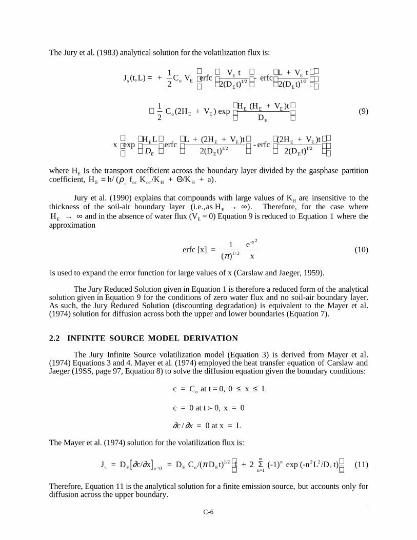
C-66
The Jury et al. (1983) analytical solution for the volatilization flux is:
J (t,L) + 1
2C V erfc
V t
2(D t)- erfc
L + V t
2(D t) s o E
E
E1/2
E
E1/2=
+
1
2 C (2H + V ) exp
H (H + V )t
Do E EE E E
E
(9)
x exp H L
erfc L + (2H + V )t
2(D t) - erfc
(2H + V )t
2(D t)E E E
E1/2
E E
E1/2DE
where HE Is the transport coefficient across the boundary layer divided by the gasphase partitioncoefficient, H h/ ( f K /K + /K + a)E oc oc H Hb
= ρ Θ .
Jury et al. (1990) explains that compounds with large values of KH are insensitive to thethickness of the soil-air boundary layer (i.e.,as H )E → ∞ . Therefore, for the case whereH E → ∞ and in the absence of water flux (VE = 0) Equation 9 is reduced to Equation 1 where theapproximation
erfc [x] = 1
e
x
-x2
( ) /π 1 2 (10)
is used to expand the error function for large values of x (Carslaw and Jaeger, 1959).
The Jury Reduced Solution given in Equation 1 is therefore a reduced form of the analyticalsolution given in Equation 9 for the conditions of zero water flux and no soil-air boundary layer.As such, the Jury Reduced Solution (discounting degradation) is equivalent to the Mayer et al.(1974) solution for diffusion across both the upper and lower boundaries (Equation 7).
2.2 INFINITE SOURCE MODEL DERIVATION
The Jury Infinite Source volatilization model (Equation 3) is derived from Mayer et al.(1974) Equations 3 and 4. Mayer et al. (1974) employed the heat transfer equation of Carslaw andJaeger (19SS, page 97, Equation 8) to solve the diffusion equation given the boundary conditions:
c = C at t = 0, 0 x Lo ≤ ≤
c = 0 at t 0, x = 0f
∂ ∂c x/ = 0 at x = L
The Mayer et al. (1974) solution for the volatilization flux is:
J = D c/ x = D C /( D t) 1 + 2 (-1) exp (-n L /D t)s E E o E1/2
n=1
n 2 2E∂ ∂ π[ ]
=
∞
x 0Σ (11)
Therefore, Equation 11 is the analytical solution for a finite emission source, but accounts only fordiffusion across the upper boundary.

C-77
The summation expression in Equation 11 decreases with increasing L and decreasing DEand t. If this term is small enough to be negligible, Equation 11 reduces to:
Js = D C /( D t)E o E1/2π (12)
Use of Equation 12 will result in less than 1 percent error if t < L2/18.4 DE (Mayer et al., 1974) .
Jury et al. (1984 and 1990) gave the solution for the semi-infinite case in Equation 3 where
C = C at t 0, x =o ≥ ∞ as:
Js = C (D / t)o E1/2π
Equation 3 is equivalent to the semi-infinite solution of Mayer et al. (1974) as given inEquation 12 and provides a bounding estimate of the maximum volatilization flux but does notaccount for source depletion. As with Equation 12, use of Equation 3 on a finite system will resultin less than 1 percent error if t < L2/18.4 DE. For the purposes of calculating SSLs based onvolatilization from soils, let t be set equal to the exposure interval. If t < L2/18.4 DE, Equation 1should be used to calculate the volatilization factor. As an alternative, an estimate of the averageemission flux over the exposure interval, <Js>, can be obtained from a simple mass balance:
< Js > = C L/to (13)
where Co = Initial soil concentration (total volume), µg/cm3-soil
L = Depth from soil surface to the bottom of contamination, cm
t = Exposure interval, days.
2 . 3 SUMMARY OF MODEL ASSUMPTIONS AND LIMITATIONS
The Jury Reduced Solution finite source volatilization model is analogous to themathematical solution for heat flow in a solid such that the region 0 < x < L is initially at constanttemperature, the region x > L is at zero, and the surface x = 0 is maintained at zero for t > 0(Carslaw and Jaeger, 1959). As such, the model's applicability to diffusion processes is limited tothe initial and boundary conditions upon which the model is derived. The following represents themajor model assumptions for these conditions:
1. Contamination is uniformly incorporated from the soil surface to depth L.
2. The soil column is isotropic to an infinite depth (i.e., uniform bulk density, soilmoisture content, porosity and organic carbon fraction).
3. Liquid water flux is zero through the soil column (i.e., no leaching or evaporation).
4. No soil-air boundary layer exists.
5. The soil equilibrium liquid-vapor partitioning (Henry's law) is instantaneous.
6. The soil equilibrium adsorption isotherm is instantaneous, linear, and reversible.

C-88
7. Initial soil concentration is in dissolved form (i.e., no residual-phasecontamination).
8. Diffusion occurs simultaneously across the upper boundary at x = 0 and the lowerboundary at x = L.
The model is therefore limited to surface contamination extending to a known depth andcannot account for subsurface contamination covered by a layer of clean soil. Also, the model doesnot consider mass flow of contaminants due to water movement in the soil nor the volatilizationrate of nonaqueous-phase liquids (residuals). Finally, the model does not account for the resistanceof a soil-air boundary layer for contaminants with low Henry's law constants.
The Jury Infinite Source volatilization model is analogous to the mathematical solution forheat flow in a semi-infinite solid. The major model assumptions are the same as those of the JuryReduced Solution finite source model except that the contamination is assumed to be uniformlyincorporated from the soil surface to an infinite depth, and that diffusion occurs only across theupper boundary.
In general, both models describe the vapor-phase diffusion of the contaminants to the soilsurface to replace that lost by volatilization to the atmosphere. Each model predicts an exponentialdecay curve over time once equilibrium is achieved. In actuality, there is a high initial flux ratefrom the soil as surface concentrations are depleted. The lower flux rate characteristics of the latterportion of the decay curve are thus determined by the rate at which contaminants diffuse upward.This type of desorption curve has been well documented in the literature. It is important to note thatboth models do not account for the high initial rate of volatilization before equilibrium is attainedand will tend to underpredict emissions during this period. Finally, each model is most applicableto single chemical compounds fully incorporated into isotropic soils. Effective solubilities andactivity coefficients in multicomponent systems are not addressed in the determination of theeffective diffusion coefficient nor is the effect of nonlinear soil adsorption and desorptionisotherms. However, because of the complexities involved with theoretical solutions to theseeffects, their contribution to model accuracy is difficult to predict, especially in multicomponentsystems.

C-99
SECTION 3
MODEL VALIDATION
To achieve the project objective, EQ executed a literature search and a survey ofprofessional environmental investigation/research firms as well as regulatory agencies to obtainexperimental and field data suitable for comparing modeled emissions with actual emissions. Theliterature search uncovered several papers and bench-scale experimental studies concerned with thevolatilization and vapor density of pesticides and chlorinated organics incorporated in soils (Farmeret al., 1972, 1974, and 1980; Spencer and Cliath, 1969 and 1970; Spencer, 1970; and Jury et al.,1980).
3.1 VALIDATION OF THE JURY INFINITE SOURCE MODEL
From the literature search, one bench-scale study was found that approximated theboundary conditions of the Jury Infinite Source model and met the data requirements for thisproject, Farmer et al., (1972). The Farmer et al. (1972) study reports the experimental emissionsof lindane (1,2,3,4,5,6-hexachlorocyclohexane, gamma isomer) and dieldrin(1,2,3,4,10,10-hexachloro-6,7-epoxy-1,4,4a,5,6,7,8,8a-octahydro-1,4-endo, exo-5, 8-dimethanonapthalene) incorporated in Gila silt loam.
The objective of the survey of professional firms and regulatory agencies was to findpilot-scale or field-scale studies of volatilization of organic compounds using the U.S. EPAemission isolation flux chamber. The candidate flux chamber studies must also have providedadequate data for input to the volatilization models.
Flux chamber studies were chosen to provide pilot-scale or field-scale measurement dataneeded for model validation. Flux chambers have been widely used to measure flux rates of VOCsand inorganic gaseous pollutants from a wide variety of sources. The flux chamber was originallydeveloped by soil scientists to measure biogenic emissions of inorganic gases and their use datesback at least two decades (Hill et al., 1978). In the early 1980's, EPA became interested in thistechnique for estimating emission rates from hazardous wastes and funded a series of projects todevelop and evaluate the flux chamber method. The initial work involved the development of adesign and approach for measuring flux rates from land surfaces. A test cell was constructed andparametric tests performed to assess chamber design and operation (Kienbusch and Ranum, 1986and Kienbusch et al., 1986). A series of field tests were performed to evaluate the method underfield conditions (Radian Corporation, 1984 and Balfour, et al., 1984). A user's guide wassubsequently prepared summarizing guidance on the design, construction, and operation of theEPA recommended flux chamber (Keinbusch, 1985). The emission isolation flux chamber ispresently considered the preferred in-depth direct measurement technique for emissions of VOCsfrom land surfaces (EPA, 1990).
EQ contacted several environmental consulting firms as well as State and local agencies. Inaddition, the EPA data base of emission flux measurement data was reviewed (EPA, 1991a).Although several flux measurement studies were found, only one applicable study was identifiedwith adequate QA/QC documentation and the necessary input data for the Jury Infinite Sourcemodel (Radian Corporation, 1989).
From Farmer et al. (1972) the influence of pesticide vapor pressure on volatilization wasmeasured by comparing the volatilization from Gila silt loam of dieldrin with that of lindane.Volatilization of dieldrin and lindane was measured in a closed airflow system by collecting thevolatilized insecticides in ethylene glycol traps. Ten grams of soil were treated with either 5 or 10µg/g of C-14 tagged insecticide in hexane. The hexane was evaporated by placing the soils in a

C-101 0
fume hood overnight. Sufficient water was then added to bring the initial soil water content to 10percent. For the volatilization studies, the treated soil was placed in an aluminum pan 5 mm deep,29 mm wide, and 95 mm long. This produced a bulk density of 0.75 g/cm3. The aluminum panwas then introduced into a 250 mL bottle which served as the volatilization chamber. A relativehumidity of 100 percent was maintained in the incoming air stream to prevent water evaporationfrom the soil surface. Air flow was maintained at 8 mL/s equivalent to approximately 0.018 milesper hour. The temperature was maintained at 30°C. The soil was a Gila silt loam, which contained0.58 percent organic carbon.
The volatilized insecticides were trapped in 25 mL of ethylene glycol. Insecticides wereextracted into hexane and anhydrous sodium sulfate was added to the hexane extract to removewater. Aliquots of the dried hexane were analyzed for lindane and dieldrin using liquidscintillation. The extraction efficiencies for lindane and dieldrin were 100 and 95 percent,respectively. The concentrations of volatilized compounds were checked using gas-liquidchromatography. All experiments were run in duplicate.
To ensure that the initial soil concentrations of lindane and dieldrin were in dissolved form,the saturation concentration (mg/kg) of both compounds under experimental conditions wascalculated using the procedures given in U.S. EPA (1994):
Csat = S
(f K + + K a )b
oc oc b Hρρ Θ (14)
where S is the pure component solubility in water. Csat for lindane and dieldrin were calculated tobe 34 mg/kg and 12 mg/kg, respectively. Therefore, the initial soil concentrations of 10 and 5mg/kg were below saturation for both compounds.
Table 1 gives the values of each variable employed to calculate the emissions of lindane anddieldrin using the Jury Infinite Source volatilization model (Equation 3). The potential for loss ofcontaminant at the lower boundary at each time-step was checked to see if t > L2/18.4 DE. If thiscondition was true at any time-step, the boundary conditions of the infinite source model wereviolated. In such a case, emissions were also calculated using the finite source model of Mayer etal. (1974) as presented in Equation 11. The difference between the predictions of both modelswere compared at each time-step and a percent error was calculated for the infinite source model.The instantaneous emission flux values predicted by Equation 3 and Equation 11 (whereapplicable) were plotted against the measured flux values for dieldrin and lindane at both 5 and 10ppmw.
Figure 1 shows the comparison of the predicted and measured values of dieldrin at an initialsoil concentration of 5 ppmw. For dieldrin, the boundary conditions of the infinite source modelwere not violated until the last time-step. A best curve was fit to both the measured and predictedvalues. As expected, both curves indicate an exponential decrease in emissions with time.
The ratio of the modeled emission flux to the measured emission flux was determined as ameasure of the relative difference between the modeled and measured values. The natural log ofthis ratio was then analyzed by using a standard paired Student's t-test. This analysis is equivalentto assuming a lognormal distribution for the emission flux and analyzing the logtransformed datafor differences between modeled and measured values.

C-111 1
TABLE 1.VOLATILIZATION MODEL INPUT VALUES FOR LINDANE AND DIELDRIN
Variable Symbol Units Value Reference/EquationInitial soilconcentration
Co mg/kg 5 and 10 Farmer et al. (1972)
Soil depth L cm 0.5 Farmer et al. (1972)Soil dry bulkdensity
ρb g/cm3 0.75 Farmer et al. (1972)
Soil particledensity
ρs g/cm3 2.65 U.S. EPA (1988)
Gravimetric soilmoisture content
w percent 10 Farmer et al. (1972)
Water-filled soilporosoty
Θ cm3/cm3 0.075 wρs
Total soil porosity φ cm3/cm3 0.717 1− ( / )ρ ρb s
Air-filled soilporosity
a cm3/cm3 0.642 φ - Θ
Soil organic carbon foc fraction 0.0058 Farmer et al. (1972)Organic carbonpartition coefficient
Koc cm3/g 1380 U.S. EPA (1994)
Diffusivity in air(Lindane)
Dga cm2/d 1521 U.S. EPA (1994)
Diffusivity in air(Dieldin)
Dga cm2/d 1080 U.S. EPA (1994)
Diffusivity in water(Lindane)
Diw cm2/d 0.480 U.S. EPA (1994a)
Diffusivity in water(Dieldrin)
Diw cm2/d 0.410 U.S. EPA (1994a)
Henry’s lawconstant (Lindane)
KH unitless 1.40 E-04 U.S. EPA (1994)
Henry’s lawconstant (Dieldrin)
KH unitless 2.75 E-06 U.S. EPA (1994)
Degradation rateconstant (Lindaneand Dieldrin)
µ 1/day 0 Default to eliminateeffects of degradation

C-121 2
Figure 1Predicted And Measured Emission Flux Of Dieldrin Versus Time (C° = 5 ppmw)

C-131 3
The data were also analyzed by using standard linear regression techniques (Figure 2).Again, the data were assumed to follow a lognormal distribution. A simple linear regression modelwas fit to the log-transformed data and the Pearson correlation coefficient was determined. ThePearson correlation coefficient is a measure of the strength of the linear association between thetwo variables.
From a limited population of four observations, the correlation coefficient was calculated tobe 0.994 with a mean ratio of modeled-to-measured values of 0.42. The actual significance(p-value) of the paired Student's t-test was p = 0.0001. The lower and upper confidence limitswere calculated to be 0.38 and 0.48, respectively. On average, this indicates that at the 95 percentconfidence limit, the modeled emission flux is between 0.38 and 0.48 times the measured emissionflux.
Figure 3 shows the modeled and measured flux values of dieldrin at an initial soilconcentration of 10 ppmw, while Figure 4 shows the relationship of the log-transformed data andthe upper and lower confidence limits. At 10 ppmw, the correlation coefficient was 0.974 with amean ratio of 0.45, p-value of 0.0001, and a 95 percent confidence interval of 0.37 to 0.54.
As can be seen from Figures 1 and 3, the model underpredicts the emissions during theinitial stages of the experiment. This is to be expected in that during this phase, contaminant isevaporating from the soil surface. The apparent discrepancy between measured and predictedvalues decreases with time as equilibrium is achieved and diffusion becomes the rate-limitingfactor.
For lindane, the boundary conditions of the infinite source model were violated after thefirst time-step (i.e., t > L2/18.4 DE at 24 hours). Therefore, the Mayer et al. (1974) finite sourcemodel was used to derive a percent error at each succeeding timestep. At an initial soilconcentration of 5 ppmw, the infinite source model predicted 114 percent total mass loss of thefinite source model over the entire time span of the experiment. At a concentration of 10 ppmw, theinfinite source model predicted 107 percent total mass loss of the finite source model.
Figures 5 and 6 show the comparison of modeled to measured values of lindane at initialsoil concentrations of 5 and 10 ppmw, respectively. Likewise, Figures 7 and 8 show thecomparisons of the log-transformed data. At an initial soil concentration of 5 ppmw, the correlationcoefficient between modeled and measured values was 0.997 with a mean modeled-to-measuredratio of 0.81, a p-value of 0.3281, and a 95 percent confidence interval of 0.46 to 1.44. At aninitial soil concentration of 10 ppmw, the correlation coefficient was calculated to be 0.998, themean ratio 0.73, the p-value 0.1774, and the confidence interval 0.41 to 1.28.
The p-values for dieldrin are considerably lower than those of lindane. This is due to thevery narrow confidence interval around the modeled values. In the case of dieldrin, Equation 3 didnot predict a loss of contaminant at the lower boundary until the last time-step (i.e., t > L2/18.4 DEat 12 days). This results in a nearly perfect straight line when the log-transformed data are plotted.For dieldrin, therefore, Equations 3 and 11 predict identical values until the last timestep.
Table 2 summarizes statistical analysis for the bench-scale comparative validation of theJury Infinite Source volatilization model. In general, the data support good agreement betweenmodeled and measured values and show relatively narrow confidence intervals and high correlationcoefficients.
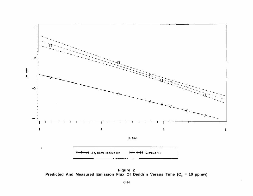
C-141 4
Figure 2Predicted And Measured Emission Flux Of Dieldrin Versus Time (Co = 10 ppmw)
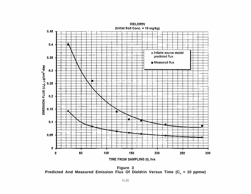
C-151 5
Figure 3Predicted And Measured Emission Flux Of Dieldrin Versus Time (Co = 10 ppmw)

C-161 6
Figure 4Comparison Of Log-Transformed Modeled And Measured Emission Flux Of Dieldrin (Co = 10 ppmw)

C-171 7
Figure 5Predicted And Measured Emission Flux Of Lindane Versus Time (Co = 5 ppmw)
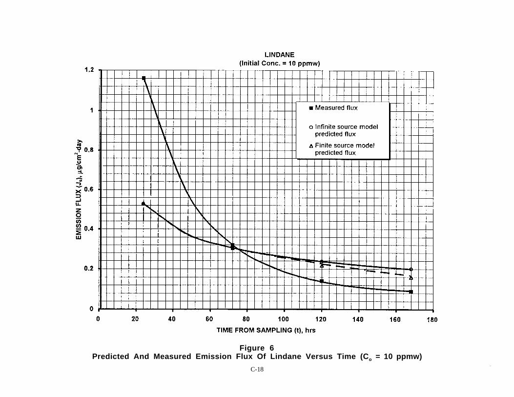
C-181 8
Figure 6Predicted And Measured Emission Flux Of Lindane Versus Time (Co = 10 ppmw)

C-191 9
Figure 7Comparison Of Log-Transformed Modeled And Measured Emission Flux Of Lindane (Co = 5 ppmw)
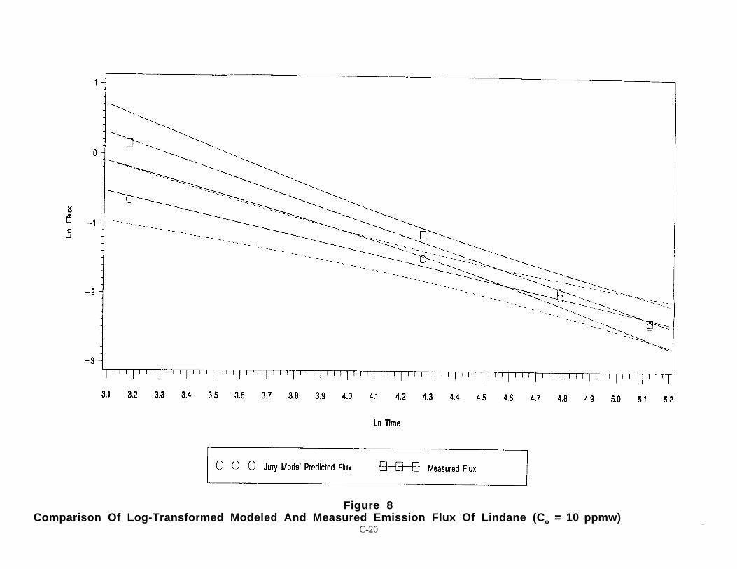
C-202 0
Figure 8Comparison Of Log-Transformed Modeled And Measured Emission Flux Of Lindane (Co = 10 ppmw)

C-212 1
TABLE 2.SUMMARY OF THE BENCH-SCALE VALIDATION OF
THE JURY INFINITE SOURCE MODEL
Chemical NCorrelationcoefficient
Mean ratio:Modeled-to-
measured p-value
9 5 %confidence
intervalLindane (5 ppmw) 4 0.997 0.81 0.3281 (0.46, 1.44)Lindane (10 ppmw) 4 0.998 0.73 0.1774 (0.41, 1.28)Dieldrin (5 ppmw) 7 0.994 0.42 0.0001 (0.38, 0.48)Dieldrin (10 ppmw) 7 0.974 0.45 0.0001 (0.37, 0.54)
Appendix A contains the spreadsheet calculations for the bench-scale validation of the JuryInfinite Source volatilization model.
From Radian Corporation (1989), a pilot-scale study was designed to determine howdifferent treatment practices affect the rate of loss of benzene, toluene, xylenes, and ethylbenzene(BTEX) from soils. The experiment called for construction of four piles of loamy sand soil, eachwith a volume of approximately 4 cubic yards (7900 pounds), a surface area of 8 square meters,and a depth of 0.91 meters. Each test cell was lined with an impermeable membrane and the soil ineach cell was sifted to remove particles larger than three-eighth inch in diameter. The contaminatedsoil for each pile was prepared in batches using 55-gallon drums. In the "high level" study, eachsoil batch was brought to 5 percent moisture content and 6 liters of gasoline added. Additionalwater was then added to bring the soil to 10 percent moisture by weight. The drums were cappedand sat undisturbed overnight. The drums were then opened the next day and shoveled into the testcell platform. Twenty-two soil batches were prepared for each soil pile. Each batch consisted of360 pounds of soil and 6.0 liters of fuel. Therefore, each soil pile contained 7900 pounds of soiland 132 liters of gasoline. Each soil pile was then subjected to one of the following managementpractices:
• A control pile that was not moved or treated
• An "aerated" or "mechanically mixed" pile
• A soil pile simulating soil venting or vacuum extraction
• A soil pile heated to 38°C.
Losses due to volatilization during the mixing and transfer process and during a 28 hourholding time in the test bed before initial sampling reduced the residual BTEX in soil. For thepurpose of this validation study, however, these losses caused initial soil concentrations ofbenzene, toluene, and ethylbenzene to be below or within a factor of two of their respective singlecomponent saturation concentrations. Because the mixed pile, vented pile, and heated pile weresubject to mechanical disturbances or thermal treatment, only the control pile data were used in thisstudy.
In general, the test schedule called for collection of soil samples and air emission lossmeasurements during the first, sixth, and seventh weeks Soil samples were collected randomlywithin specified grid areas by composite core collection to the maximum depth of the pile.Emission losses were measured similarly using an emission isolation flux chamber as specified inKienbusch (1985). Only data for which soil samples and flux chamber measurements were takenon the same day were used for this study.
C-222 2
Analysis of BTEX in soil samples was accomplished by employing the EPA 5030extraction method and the EPA 8020 analytical method. The BTEX method was modified to reducethe sample hold time to one day in an effort to improve the accuracy of the method. Five soilsamples were submitted in duplicate. The relative percent differences (RPD) ranged from 8.0 to48.9 percent. The average RPD for the five samples was 26.8 percent. In addition, EPA QCsample analysis indicated average percent recoveries ranging from 89 percent for m-xylene to 119percent for toluene. The pooled coefficient of variation (CV) for all the BTEX analysis was 10.5percent. Spiked sample recoveries (eight samples) ranged from 75 percent for m-xylene to 168percent for toluene. The average spike recoveries ranged from 108 percent for benzene to 146percent for toluene. Finally, both system blanks and reagent blanks indicated no contamination wasfound in the analytical system.
It should be noted that the standard method used for BTEX analysis was observed to havecontributed to the variabilities in soil concentrations. The EPA acceptance criteria based on 95percent confidence intervals from laboratory studies are roughly 30 to 160 percent for the BTEXcompounds during analysis of water samples. The necessary extraction step for soil sampleswould increase this already large variability.
Analysis of vapor-phase organic compounds via the emission isolation flux chamber wasaccomplished using a gas chromatograph (GC). Gas samples were collected from the flux chamberin 100 mL, gas-tight syringes and analyzed by the GC in laboratory facilities adjacent to the testsite. During the study, a multicomponent standard was analyzed daily to assess the precision anddaily replication of the analytical system. The results of the analysis indicated a good degree ofreproducibility with coefficients of variation ranging from 5.1 to 16.3 percent.
From these data, instantaneous emission fluxes were calculated for benzene, toluene, andethylbenzene corresponding to each time period at which flux chamber measurements were made.Table 3 gives the values of each variable employed to calculate emissions of each compound usingthe Jury Infinite Source model and the Mayer et al. (1974) finite source model. Appendix Acontains the spreadsheet data for benzene, toluene, and ethylbenzene at initial soil concentrations of110 ppm, 880 ppm, and 310 ppm, respectively.
It should be noted that the fraction of soil organic carbon (foc) was not available fromRadian (1989). For this reason, the default value for foc of 0.006 from U.S. EPA (1994) was usedfor all calculations.
Figures 9, 10, and 11 show the comparison of modeled and measured emission fluxes ofbenzene, toluene, and ethylbenzene, respectively. The Radian Corporation study noted that thesecond measured value in each figure represented a data outlier, possibly due to the formation of asoil fissure, reducing the soil path resistance and increasing the emission flux.
Table 4 presents the results of the statistical analysis of the comparison of modeled andmeasured values. For both benzene and ethylbenzene, measured values were below the detectionlimits after the fifth observation; measured values for toluene were below the detection limit afterthe seventh observation.

C-232 3
TABLE 3.VOLATILIZATION MODEL INPUT VARIABLES FOR BENZENE,
TOLUENE, AND ETHYLBENZENE
Variable Symbol Units Value Reference/EquationInitial soil concentration
- benzene- toluene- ethylbenzene
Co mg/kg110880310
Radian (1989)
Soil Depth L cm 91 Radian (1989)Soil dry bulk density ρb g/cm3 1.5 Radian (1989)Soil particle density ρs g/cm3 2.65 U.S. EPA (1988)Gravimetric soil moisturecontent
w percent 10 Radian (1989)
Water-filled soil porosoty Θ cm3/cm3 0.150 wρb
Total soil porosity φ cm3/cm3 0.434 1− ( / )ρ ρb s
Air-filled soil porosity a cm3/cm3 0.284 φ - ΘSoil organic carbon foc Fraction 0.006 U.S. EPA (1994) default
valueOrganic carbon partitioncoefficient
- benzene- toluene- ethylbenzene
Koc cm3/g
57131221
U.S. EPA (1994)U.S. EPA (1994)U.S. EPA (1994)
Diffusivity in air- benzene- toluene- ethylbenzene
Dga cm2/s
0.08700.08700.0750
U.S. EPA (1994)U.S. EPA (1994)U.S. EPA (1994)
Diffusivity in water- benzene- toluene- ethylbenzene
Diw cm2/s
9.80 E-068.60 E-068.64 E-06
U.S. EPA (1994a)U.S. EPA (1994a)U.S. EPA (1994a)
Henry’s law constant- benzene- toluene- ethylbenzene
KH Unitless0.220.260.32
U.S. EPA (1994)U.S. EPA (1994)U.S. EPA (1994)
Degradation rate constant µ 1/day 0 Default to eliminateeffects of degradation

C-242 4
Figure 9Predicted And Measured Emission Flux Of Benzene (Co = 110 ppmw)
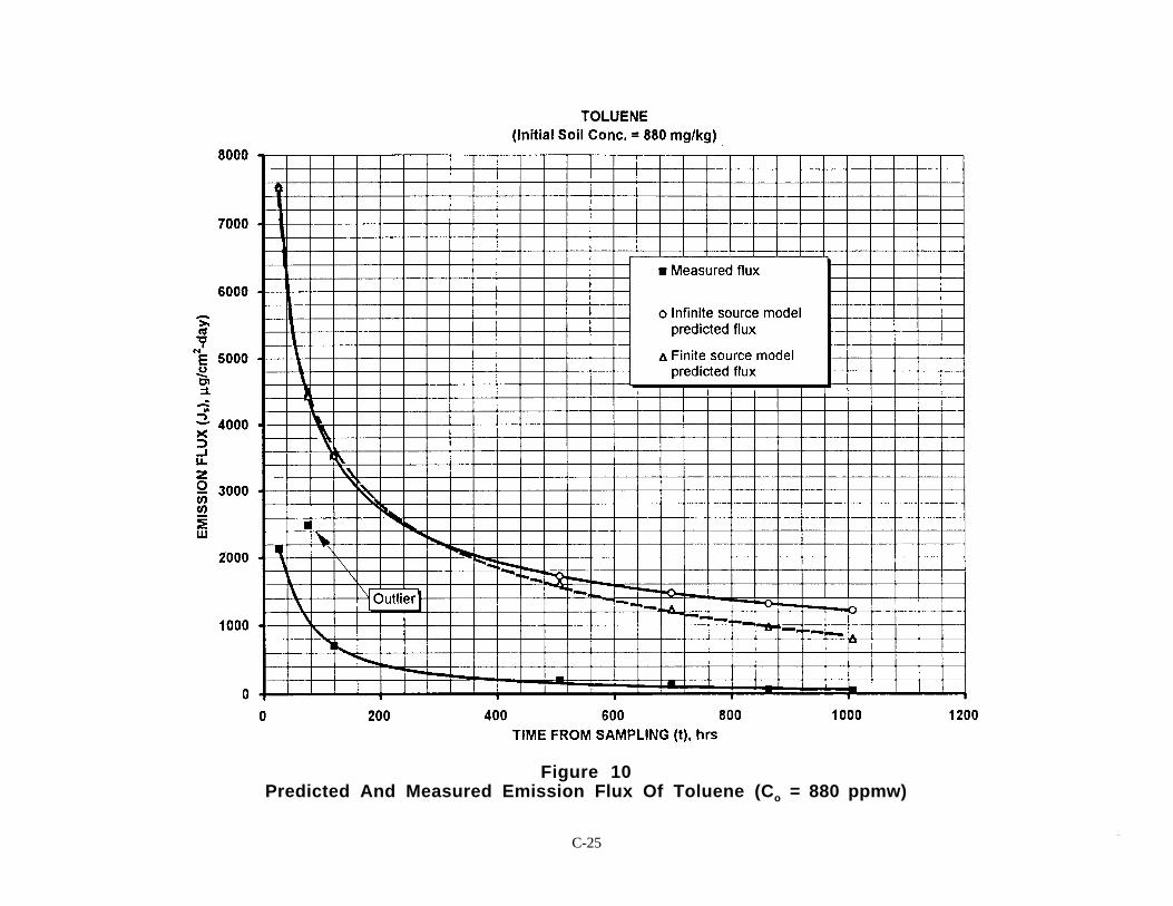
C-252 5
Figure 10Predicted And Measured Emission Flux Of Toluene (Co = 880 ppmw)
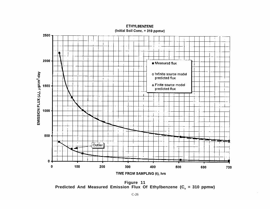
C-262 6
Figure 11Predicted And Measured Emission Flux Of Ethylbenzene (Co = 310 ppmw)

C-272 7
TABLE 4.SUMMARY OF STATISTICAL ANALYSIS OF PILOT-SCALE VALIDATION
Chemical NCorrelationcoefficient
Mean ratio:Modeled-to-
measured p-value
9 5 %confidence
intervalBenzene (110 ppm) 5 0.982 2.5 0.0149 (1.4, 4.5)Toluene (880 ppm) 7 0.988 6.3 0.0002 (3.9, 10.4)Ethylbenzene (310 ppm) 5 0.999 7.8 0.0008 (4.9, 12.4)
Figures 12, 13, and 14 show the comparison of the log-transformed data for the modeledand measured emission fluxes of benzene, toluene, and ethylbenzene, respectively. As can be seenfrom Table 4, correlation coefficients ranged from 0.982 for benzene to 0.999 for ethylbenzene,while p-values and 95 percent confidence intervals indicate a significant statistical differencebetween modeled and measured values.
The boundary conditions of the infinite source model were violated after the first timestepfor benzene, and after the third time-step for both toluene and ethylbenzene. The infinite sourcemodel predicted 134 percent, 117 percent, and 103 percent of the total mass loss of the finitesource model for benzene, toluene, and ethylbenzene, respectively.
In general, the predicted values were higher than the measured values throughout thetime-span of the experiment for all three compounds. It is also interesting to note that during theinitial stage of the experiment the predicted values were considerably higher than measured valueseven when contaminant loss at the soil surface due to evaporation was expected. Although therelative differences between predicted and measured values are not excessive (i.e., the highestmodeled-to-omeasured mean ratio is within a factor of approximately 10), they are considerablyhigher than those of the bench-scale studies.
Any one or a combination of the following could account for the larger discrepanciesbetween measured and predicted values in the pilot-scale study:
1. Although the initial soil concentrations of the three compounds were below orwithin a factor of two of their respective single component saturationconcentrations, they may have been greater than the component concentrations forwhich a residual-phase of gasoline existed. If this were the case, measuredemissions may have been in part due to the presence of nonaqueous-phase liquids(NAPL) which would have violated the model's assumptions of equilibriumpartitioning.
2. Soil mixing processes and transfer to the test bed may have resulted inheterogenous incorporation of the contaminants. If surface concentrations werereduced due to incomplete mixing, measured emissions would have been reducedduring the initial stages of the experiment.
3. Sampling and/or analytical variability may have resulted in under reporting ofemission fluxes and/or over reporting of initial soil concentrations.
4. Contaminants sorbed to the test bed liner may have acted to reduce emissions.

C-282 8
Figure 12Comparison Of Log-Transformed Modeled And Measured Emission Flux Of Benzene (Co = 110 ppmw)

C-292 9
Figure 13Comparison Of Log-Transformed Modeled And Measured Emission Flux Of Toluene (Co = 880 ppmw)

C-303 0
Figure 14Comparison Of Log-Transformed Modeled And Measured Emission Flux Of Ethylbenzene (Co = 310 ppmw)

C-313 1
5. Variability in the relative humidity of the air above the test bed may have inducedsurface water evaporation in between flux chamber samples. Water evaporationwould have moved contaminants to the surface by convection and depleted soilconcentrations in between sampling events.
6. The model is not as accurate for compounds with relatively high Henry's lawconstants.
From these observations, it appears more likely that the larger discrepancies betweenmodeled and measured emissions in the pilot-scale study are due to experimental conditions.Sufficient uncertainty exists as to whether all model boundary conditions were maintained duringthe experiment. For this reason, the results of the pilot-scale validation should be considered lessreliable than those of the bench-scale validation. This conclusion suggests that controlled studiesshould be considered for validation of model predictions for compounds with relatively highHenry's law constants.
3.2 VALIDATION OF THE JURY REDUCED SOLUTION FINITESOURCE MODEL
From the literature search, one bench-scale study was found that replicated the boundaryconditions of the Jury Reduced Solution model (Equation 1). Jury et al. (1980) reports theemissions of the herbicide triallate [S-(2,3,3-trichloroallyl) diisopropyithiocarbamate] incorporatedin San Joaquin sandy loam. This study replicated the model boundary conditions in that a cleanlayer of soil underlayed the contaminated soil allowing diffusion across the lower boundary as wellas the upper boundary.
Volatilization of triallate was measured in a closed volatilization chamber (Spencer et al., 1979).The air chamber above the soil was 2 mm deep and 3 cm wide, matching the width of theevaporating surface. An average air flow rate of 1 liter per minute was maintained across thesurface equivalent to a windspeed of 1 km/h. Triallate was applied by atomizing the material inhexane onto the air-dry autoclaved soil. The soil was mixed and allowed to equilibrate in a ventedfume hood. The soil was then transferred to the chamber and wetted from the bottom. To preventwater evaporation at the soil surface, the chamber was maintained at 100 percent relative humidityand a temperature of 25°C.
The volatilized triallate was trapped daily on polyurethane plugs and extracted and analyzed asdescribed in Grover et al. (1978). The volatilization of triallate at an initial soil concentration of 10ppmw was measured over a 29 day period in the absence of water evaporation. Calculation of thesaturation concentration (Csat) confirmed that the initial concentration of 10 ppmw was in dissolvedform. Table 5 gives the values of each variable employed to calculate emissions of triallate usingthe Jury Reduced Solution volatilization model.
Figure 15 shows the comparison of the predicted and measured values for triallate at aninitial soil concentration of 10 ppmw. The data plots indicate very good agreement betweenmodeled and measured values. Figure 16 shows the comparison of the log-transformed data andconfidence intervals. From the population of 32 observations, the correlation coefficient wascalculated to be 0.998 with a mean modeled-to-measured ratio of 1.11. The p-value was calculatedat 0.0001, and the confidence interval was 1.07 to 1.16.

C-323 2
TABLE 5.VOLATILIZATION MODEL INPUT VALUES FOR TRIALLATE
Variable Symbol Units Value Reference/EquationInitial soil concentration Co mg/kg 10 Jury et at. (1980)Soil depth L cm 10 Jury et at. (1980)Soil dry bulk density ρb g/cm3 1.34 Jury et at. (1980)Soil particle density ρs g/cm3 2.65 U.S. EPA (1988)Gravimetric soil moisture content w percent 21 Calculated from Jury et al.
(1980)Water-filled soil porosoty Θ cm3/cm3 0.279 Jury et at. (1980)Total soil porosity φ cm3/cm3 0.494 Jury et at. (1980)Air-filled soil porosity a cm3/cm3 0.215 Jury et at. (1980)Soil organic carbon foc fraction 0.0072 Calculated from Jury et al.
(1980)Organic carbon partitioncoefficient
Koc cm3/g 3600 Jury et at. (1980)
Diffusivity in air Dga cm2/d 3888 Jury et at. (1980)
Diffusivity in water Diw cm2/d 0.432 Jury et at. (1980)
Henry’s law constant KH unitless 1.04 E-03 Jury et at. (1980)Degradation rate constant µ 1/day 0 Default to eliminate
effects of degradation
The degree of agreement between modeled and measured emission flux values for triallatemay be due to soil adsorption studies conducted to experimentally derive the organic carbonpartition coefficient specific to the San Joaquin sandy loam used in the experiment. Withexperimentally derived values of Koc, more accurate phase partitioning was possible resulting in anexperimental-specific value of the effective diffusion coefficient (Equation 2). Appendix B containsthe spreadsheet calculations for the bench-scale validation of the Jury Reduced Solution finitesource volatilization model.
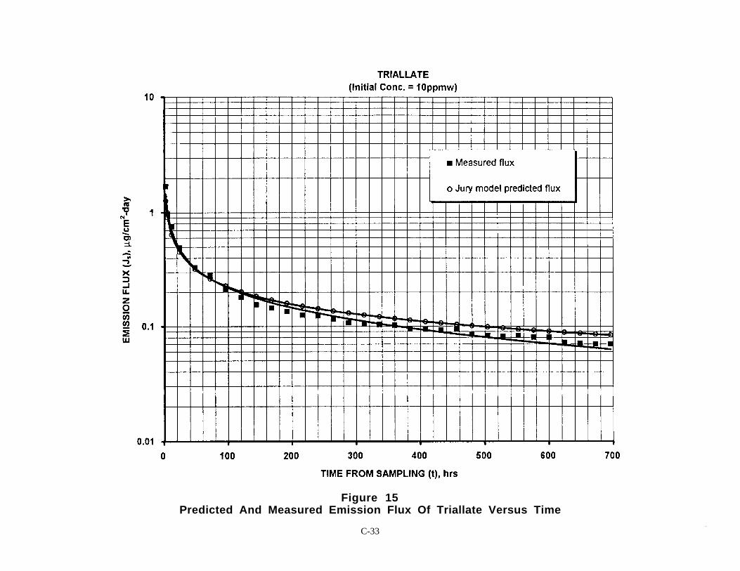
C-333 3
Figure 15Predicted And Measured Emission Flux Of Triallate Versus Time

C-343 4
Figure 16Comparison Of Log-Transformed Modeled And Measured Emission Flux Of Triallate

C-353 5
SECTION 4
PARAMETRIC ANALYSIS OF THE JURYVOLATILIZATION MODELS
This section presents the results of parametric analysis of the key variables of the Juryvolatilization models (Equations 1 and 3). The Jury volatilization models are applicable for the caseof no boundary layer resistance at the soil-air interface and no water flux through the soil column.Because the models are equivalent to the Mayer et al. (1974) solutions to the general diffusionequation (Equation 5), the parametric observations of Mayer et al. (1974) and Farmer, et al. (1980)are also directly applicable.
Jury et al. (1983) established the relationship between vapor and solute diffusion andadsorption by defining total phase concentration partitioning as it relates to the effective diffusioncoefficient. The effective diffusion coefficient is a theoretical expression of the combination of soilparameters and chemical properties which govern the rate at which soil contaminants move to thesurface to replace those lost by evaporation. As such, the effective diffusion coefficient is therate-limiting factor governing the general diffusion equation in soils given the initial and boundaryconditions for which the models are applicable. The remainder of this section discusses the key soiland nonsoil parameters used in the expression of the effective diffusion coefficient and the generaldiffusion equation.
4.1 AFFECTS OF SOIL PARAMETERS
In this section, the experimental results of Farmer, et al. (1980) are discussed as they relateto the effect of soil water content, soil bulk density, air-filled soil porosity, and temperature ondiffusion in soil.
Soil Moisture Content
Farmer, et al. (1980) indicates that the effect of soil moisture content on the volatilizationflux of contaminants through soils is exponential. Increasing soil water content decreases the porespaces available for vapor diffusion and will decrease volatilization flux. In contrast, increasingsoil water content has also been shown to increase the volatility of pesticides in soil under certainconditions (Gray, et al., 1965; and Spencer and Cliath, 1969 and 1970). In essence, the soil watercontent affects the contaminant adsorption capacity by competing for soil adsorption sites. Underthese conditions, an increase in soil moisture above a certain point will tend to desorbcontaminants, increasing the flux dependent on the relative water and contaminant adsorptionisotherms.
Bulk Density
Soil compaction or bulk density also determines the porosity of soil and thus affects thediffusion through the soil. Experimental results from Farmer et al. (1980) indicate that soil bulkdensity also has an exponential effect on volatilization flux through the soil. From previousconsiderations of the effect of soil water content, a higher bulk density will have similar effects tothat of an increased soil moisture content.
Soil Air-Filled Porosity
The effects of soil water content and soil bulk density on volatilization can be contributed totheir effect on the air-filled porosity, which in turn is the major soil factor controlling volatilization.The effect of air-filled porosity is manifested in the expression of the effective diffusion coefficient.The effective diffusion coefficient, however, does not depend only on the amount of air-filled pore
C-363 6
space. The presence of liquid film on the solid surfaces not only reduces porosity, but alsomodifies the pore geometry increasing tortuosity and the length of the gas passage. The Jury et al.(1983) expression of the effective diffusion coefficient uses the model of Millington and Quirk(1961) to account for the porosity and the tortuosity of soil as a porous medium.
Soil Temperature
The effect of soil temperature on the volatilization flux is multifunctional. The diffusion inair, Dg
a , is theoretically related to temperature, T, and the collision integral, Ω, in the followingmanner (Lyman, et al., 1990):
Dga (proportional to)
T
(T)
0.5
Ω(15)
The exponential coefficient for temperature varies from 1.5 to 2 over a wide range oftemperatures. Barr and Watts (1972) found that 1.75 gave the best values for gaseous diffusion.Farmer, et al. (1980) estimates the effective diffusion coefficient at temperature T2 as:
D2 = D1 (T2 /T1)0.5 (16)
where D2 = Diffusion coefficient at T2
D1 = Diffusion coefficient at T1
T = Absolute temperature.
A temperature increase will effect the vapor pressure function of the Henry's Law constant,which causes an increase in the vapor concentration gradient across the soil layer. In actual fact,temperature gradients will exist across the soil due primarily to seasonal variations. Vapordiffusion is influenced by such gradients; however, these effects of fluctuating soil temperatureswill tend to cancel one another over time.
4.2 AFFECTS OF NONSOIL PARAMETERS
The nonsoil variables in the Jury volatilization models include the initial soil concentration,Co, the Henry's law constant (KH), the soil/water partition coefficient, (KD) and the depth ofcontaminant incorporation (L).
Initial Soil Concentration
The effect of change in the initial soil concentration is linear; i.e., an increase in Co of 100percent causes an increase in the emission rate of 100 percent. Probably the greatest degree ofuncertainty in the value of Co is likely to be either insufficient soil sampling to adequatelycharacterize site soil concentrations, or the variability in percent recovery of contaminants as itapplies to existing sampling and analysis methods for organic compounds in soils. Typically,present extraction and analysis method recovery variability increases the likelihood ofunderprediction of the emission rate (i.e., more contaminant is present in the soil than is reportedby sampling and analysis methods).

C-373 7
Henry's Law Constant and Soil/Water Partition Coefficient
Jury et al. (1984) showed that a given chemical can be grouped into three main categoriesdepending on the ratio KD/KH. These categories are defined as a function of which phase dominatesdiffusion. A Category I chemical is dominated by the vapor-phase, a Category III chemical by theliquid-phase, and Category II chemicals by vapor-phase diffusion at low soil water content andliquid-dominated at high water content. Desorption from the solid-phase to the liquid-phase is afunction of the soil/water partition coefficient, while volatilization from the liquid to thevapor-phase is a function of the Henry's law constant. Therefore, the interstitial vapor density, andthus emission flux, is directly proportional to KH and inversely proportional to KD. Because theJury volatilization models do not account for a soil-air boundary layer, the effects of KH and KD areexponential for all three categories of chemicals.
Depth of Contaminant Incorporation
The Jury Reduced Solution finite source model accounts for diffusion across both theupper and lower boundaries. Therefore for chemicals with high effective diffusion coefficients, theresidual soil concentration will decrease rapidly. In this regard, the emission flux curve willbecome asymptotic more rapidly than for the semi-infinite case (Equation 3). The exponential term[1 - exp (-L2/4 DEt)] in Equation 1 accounts for diffusion across the lower boundary such that theterm decreases rapidly with time for small values of L and large values of DE.

C-383 8
SECTION 5
CONCLUSIONS
From the results of this study, it can be concluded that for the compounds included in theexperimental data, both models showed good agreement with measured data given the conditionsof each test. Each model demonstrated superior agreement with bench-scale measured values andto a lesser extent the infinite source model with pilot-scale data. The results indicate highcorrelation coefficients across all experimental data with mean modeled-to-measured ratios as lowas 0.37 and as high as 7.8.
From a review of test conditions, it was concluded that the bench-scale studies betterapproximated the initial and boundary conditions of the infinite source model. This is evident in thelower modeled-to-measured mean ratios and narrow 95 percent confidence intervals. Although thepilot-scale study data showed reasonable agreement with predicted values, questions remain as towhether the test conditions were in agreement with model assumptions and accurately replicated allmodel boundary conditions. Overall, each model provided reasonably accurate predictions.
Clearly, this validation study is limited by the range of conditions simulated, theassumptions under which the models operate, and the initial and boundary conditions of eachmodel. Important limitations include:
1. The duration of the experiments examined range from 7 to 36 days. Modelperformance for longer periods could not be validated.
2. Both models assume no mass flow of contaminants due to water movement in thesoil. Mass flow due to capillary action or redistribution of contaminates due to rainevents may be significant if applicable to site-specific condition.
3. The models are valid only if the effective diffusion coefficient in soil is constant.This assumes isotropic soils and completely homogeneous incorporation ofcontaminants. In reality, soils are usually heterogeneous, with properties thatchange with depth (e.g., fraction of organic carbon, water content, porosity, etc.).The user will need to carefully consider the characterization of soil properties beforeassigning model input parameters.
4. The equilibrium partitioning relationships used in the models are no longer valid forpure-phase chemicals or when high dissolved concentrations are present.Therefore, the models should not be used when these conditions exist.
5. The models do not consider the effects of a soil-air boundary layer on thevolatilization rate. For chemicals with Henry's law constants less thanapproximately 2.5 x 10⁻⁵, volatilization is highly dependent on the thickness of theboundary layer (Jury et al., 1984). A boundary layer will restrict volatilization if themaximum flux through the boundary layer is small compared to the rate at whichthe contaminant moves to the surface. In this case, the volatilization rate is inverselyproportional to the boundary layer thickness.
6. In the case of the infinite source model, validation for chemicals with relatively highHenry's law constants requires that the depth of contamination be sufficient toprevent loss at the lower boundary over the duration of the experiment, i.e., L >(18.4 DE t)1/2. Although this study indicates that the Jury Infinite Source modelexhibited a relatively small maximum error (i.e., 134% of the Mayer et al. finitesource model total mass loss for benzene), any future validation studies should

C-393 9
maintain a sufficient depth of incorporation to prevent violation of the modelboundary conditions.
7. No experimental data could be found in the literature for validation of the JuryReduced solution finite source model for compounds with high Henry's lawconstants.
Emission rates predicted by the Jury Infinite Source volatilization model and the JuryReduced Solution finite source volatilization model indicate good correlation to measured emissionrates under controlled conditions, but predicted values for field conditions would be subject toerror because the boundary conditions and environmental conditions are not as well defined as theyare in the laboratory. Nonetheless, results of this study indicate that both models should makereasonable estimates of loss through volatilization at the soil surface given the boundary conditionsof each model.

C-404 0
REFERENCES
Balfour, W. D., B. M. Eklund, and S. J. Williamson. Measurement of Volatile Organic Emissionsfrom Subsurface Contaminants. In Proceedings of the National Conference on Management ofUncontrolled Hazardous Waste Sites. September 1984, pp. 77-81. Hazardous Materials ControlResearch Institute, Silver-Springs, Maryland.
Barr, R. F. and H. F. Watts. 1972. Diffusion of Some Organic and Inorganic Compounds in Air.J. Chem. Eng. Data 17:45-46.
Carslaw, H. S., and J. C. Jaeger. 1959. Conduction of Heat in Solids. zd Edition OxfordUniversity Press, Oxford.
Environmental Quality Management, Inc. 1994. A Comparison of Soil Volatilization Models inSupport of Superfund Soil Screening Level Development. U.S. Environmental Protection Agency,Contract No. 68-D30035, Work Assignment No. 0-25.
Farmer, W. J., K. Igue, W. F. Spencer, and J. P. Martin. 1972. Volatility of OrganochlorineInsecticides from Soil. I and II Effects. Soil Sci. Soc. Amer. Proc. 36:443-450.
Farmer, W. J., and J. Letey. 1974. Volatilization Losses of Pesticides From Soils. Office ofResearch and Development. EPA-660/2-74/054.
Farmer, W. J., M. S. Yang, J. Letey, and W. F. Spencer. 1980. Land Disposal ofHexachlorobenzene Wastes. Office of Research and Development. EPA-600/2-80/119.
Gray, R. A., and A. J. Weierch. 1965. Factors Affecting the Vapor Loss of EPTC from Soil.Weeds 13:141-147.
Grover, R., W. F. Spencer, W. J. Farmer, and T. D. Shoup. 1978. Triallate Vapor Pressure andVolatilization from Glass Surfaces. Weed Sci., 26:505-508.
Hill, F. B., V. P. Aneja, and R. M. Felder. 1978. A Technique for Measurement of BiogenicSulfur Emission Fluxes. J. Env. Sci. Health AIB (3), pp. 199-225.
Howard, P. H., R. S. Boethling, W. F. Jarvis, W. M. Meylan, and E. O. Michaelenko. 1991.Handbook of Environmental Degradation Rates. Lewis Publishers, Chelsea, Michigan.
Jury, W. A., R. Grover, W. F. Spencer, and W. J. Farmer. 1980. Modeling Vapor Losses ofSoil-lncorporated Triallate. Soil Science Society Am. J., 44:445-450.
Jury, W. A., W. F. Spencer, and W. J. Farmer. 1983. Behavior Assessment Model of TraceOrganics in Soil: I. Model Description. J. Environ. Qual., Vol. 12, No. 4:558:564.
Jury, W. A., W. J. Farmer, and W. F. Spencer. 1984. Behavior Assessment Model for TraceOrganics in Soil: II. Chemical Classification and Parameter Sensitivity. J. Environ. Qual., Vol. 13,No. 4:567-572.
Jury, W. A., D. Russo, G. Streile, and H. El Abd. 1990. Evaluation of Volatilization by OrganicChemicals Residing Below the Soil Surface. Water Resources Res., Vol. 26, No. 1:13-20.
Kienbusch, M. Measurement of Gaseous Emission Rates from Land Surfaces Using an EmissionIsolation Flux Chamber - User's Guide. Report to EPA-EMSL, Las Vegas under EPA ContractNo. 68-02-3889, Work Assignment No. 18, December 1985.
C-414 1
Kienbusch, M. and D. Ranum. 1986. Validation of Flux Chamber Emission Measurements onSoil Surface - Draft Report to EPA-EMSL, Las Vegas, Nevada.
Kienbusch, M., W. D. Balfour, and S. Williamson. The Development of an Operations Protocolfor Emission Isolation Flux Chamber Measurements on Soil Surfaces. Presented at the 79thAnnual Meeting of the Air Pollution Control Association (Paper 86-20.1), Minneapolis,Minnesota, June 22-27, 1986.
Lyman, W. J., W. F. Reehl, and D. H. Rosenblatt. 1990. Handbook of Chemical PropertyEstimation Methods. American Chemical Society, Washington, D.C.
Millington, R. J., and J. M. Quirk. 1961. Permeability of Porous Solids. Trans. Faraday Soc.57:1200-1207.
Radian Corporation. Soil Gas Sampling Techniques of Chemicals for Exposure Assessment - DataVolume. Report to EPA-EMSL, Las Vegas under EPA Contract No. 68-02-3513, WorkAssignment No. 32, March 1984.
Radian Corporation. Short-term Fate and Persistence of Motor Fuels in Soils. Report to theAmerican Petroleum Institute, Washington, D.C. July 1989.
Spencer, W. F., M. Cliath, and W. J. Farmer. 1969. Vapor Density of Soil Applied HEOD asRelated to Soil Water Content, Temperature, and HEOD Concentration. Soil Sci. Soc. Amer.Proc. 33:509-511.
Spencer, W. F., and M. Cliath. 1970. Vapor Density and Apparent Vapor Pressure of Lindane(γ-BHC). J. Agr. Food Chem. 18:529-530.
Spencer, W. F., T. D. Shoup, M. M. Cliath, W. J. Farmer, and R. Haque. 1979. VaporPressures and Relative Volatility of Ethyl and Methyl Parathion. J. Agric. Food Chem.,27:273-278.
Spencer, W. F. 1970. Distribution of Pesticides Between Soil, Water and Air. In Pesticides in theSoil: Ecology, Degradation and Movement. A symposium, February 25-27, 1970. Michigan StateUniversity.
U.S. Environmental Protection Agency. 1988. Superfund Exposure Assessment Manual. Office ofEmergency and Remedial Response. EPA-540/1-88-001.
U.S. Environmental Protection Agency. 1990. Procedures for Conducting Air Pathway Analysesfor Superfund Activities, Interim Final Documents: Volume 2 - Estimation of Baseline AirEmissions at Superfund Sites. Office of Air Quality Planning and Standards. EPA-450/1-89-002a.
U.S. Environmental Protection Agency. 1991. Risk Assessment Guidance for Superfund, Volume1, Human Health Evaluation Manual (Part B). Office of Emergency and Remedial Response.Publication No. 9285.7-01B.
U.S. Environmental Protection Agency. 1991a. Database of Emission Rate Measurement Projects- Technical Note. Office of Air Quality Planning and Standards. EPA-450/1 -91 003.
U.S. Environmental Protection Agency. 1994. Technical Background Document for SoilScreening Guidance - Review Draft. Office of Solid Waste and Emergency Response. EPA-540/R-94/102.

C-424 2
U.S. Environmental Protection Agency. 1994a. CHEMDAT8 Data Base of Compound Chemicaland Physical Properties. Office of Air Quality Planning and Standards Technology TransferNetwork, CHIEF Bulletin Board. Research Triangle Park, North Carolina.

C-434 3
APPENDIX A
VALIDATION DATA FOR THE JURY INFINITE SOURCE MODEL

C-444 4
DIELDRIN 5 PPM(1 of 2)
ChemicalSamplePoint
Initial soilconc.,
Initial soilconc.,
Emittingarea
SoilDepth Soil Type
Soil bulkdensity,
Soilparticledensity,
Gravimetricsoil moisture,
Water-filled soilporosity, Solubility
Soilorganiccarbon,
Saturationconc., Co>Csat
Measuredemission
flux
Organiccarbon part.
coeff.,
Co Co ( L ) ρb ρs w Θ S fo c Csat (µg/m2 - Koc
(mg/kg) (g /g ) (cm2 ) (cm) Kg /L Kg /L (wt. fraction) (unitless) (mg/L) (fraction) (mg/kg) (Yes/No) min) (cm3 / g )
Dieldrin 1 5 5.00E-06 27.55 0.5 GilaSlit Loam 0.75 2.65 0.10 0.0750 0.1870 0.0058 12 No 200 10900Dieldrin 2 5 5.00E-06 27.55 0.5 Gila Slit Loam 0.75 2.65 0.10 0.0750 0.1870 0.0058 12 No 115 10900Dieldrin 3 5 5.00E-06 27.55 0.5 Gila Slit Loam 0.75 2.65 0.10 0.0750 0.1870 0.0058 12 No 75 10900Dieldrin 4 5 5.00E-06 27.55 0.5 Gila Slit Loam 0.75 2.65 0.10 0.0750 0.1870 0.0058 12 No 65 10900Dieldrin 5 5 5.00E-06 27.55 0.5 Gila Slit Loam 0.75 2.65 0.10 0.0750 0.1870 0.0058 12 No 60 10900Dieldrin 6 5 5.00E-06 27.55 0.5 Gila Slit Loam 0.75 2.65 0.10 0.0750 0.1870 0.0058 12 No 55 10900Dieldrin 7 5 5.00E-06 27.55 0.5 Gila Slit Loam 0.75 2.65 0.10 0.0750 0.1870 0.0058 12 No 40 10900

C-454 5
DIELDRIN 5 PPM(2 of 2)
ChemicalSoil/water part.
coeff.,Diffusivity in
air,Diffusivity in
water,
Effectivediffusion
coefficient,Henry’s law
constant,Total soilporosity,
Air-filled soilporosity,
Measured emissionflux emission flux Time, t t > L 2 /14.4 DE
Infinite sourcemodel emission
fluxKD Dg
a Diw DE KH φ a Cumulative
(cm3 / g ) (cm2 /s ) (cm2 /s ) (cm2 /s ) (unitless) (unitless) (unitless) (µg/cm2 -day) (hours) (Yes/No) (µg/cm2 -day)
Dieldrin 63.22 0.0125 4.74E-06 1.32E -08 0.00011 0.7170 0.6420 0.2000 24 No 0.0714Dieldrin 63.22 0.0125 4.74E-06 1.32E -08 0.00011 0.7170 0.6420 0.1150 72 No 0.0412Dieldrin 63.22 0.0125 4.74E-06 1.32E -08 0.00011 0.7170 0.6420 0.0750 120 No 0.0319Dieldrin 63.22 0.0125 4.74E-06 1.32E -08 0.00011 0.7170 0.6420 0.0650 144 No 0.0292Dieldrin 63.22 0.0125 4.74E-06 1.32E -08 0.00011 0.7170 0.6420 0.0600 168 No 0.0270Dieldrin 63.22 0.0125 4.74E-06 1.32E -08 0.00011 0.7170 0.6420 0.0550 216 No 0.0238Dieldrin 63.22 0.0125 4.74E-06 1.32E -08 0.00011 0.7170 0.6420 0.0400 288 No 0.0206

C-464 6
DIELDRIN 10 PPM(1 of 2)
ChemicalSamplePoint
Initial soilconc.,
Initial soilconc.,
Emittingarea
SoilDepth Soil Type
Soil bulkdensity,
Soilparticledensity,
Gravimetricsoil moisture,
Water-filled soilporosity, Solubility,
Soilorganiccarbon,
Saturationconc., Co>Csat
Measuredemission
flux
Organiccarbonpart.
coeff.,Co Co ( L ) ρb ρs w Θ S fo c Csat (ng/cm 2 Koc
(mg/kg) (g /g ) (cm2 ) (cm) (g/cm3 ) (g/cm3 ) (wt. fraction) (unitless) (mg/L) (fraction) (mg/kg) (Yes/No) -day) (cm3 / g )
Dieldrin 1 10 1.00E -05 27.55 0.5 Gila Silt Loam 0.75 2.65 0.10 0.0750 0 1870 0.0058 12 No 400 10900
Dieldrin 2 10 1.00E -05 27.55 0.5 Gila Silt Loam 0.75 2.65 0.10 0.0750 0.1870 0.0058 12 No 260 10900
Dieldrin 3 10 1.00E -05 27.55 0.5 Gila Silt Loam 0.75 2.65 0.10 0.0750 0.1870 0.0058 12 No 140 10900
Dieldrin 4 10 1.00E -05 27.55 0.5 Gila Silt Loam 0.75 2.65 0.10 0.0750 0.1870 0.0058 12 No 110 10900
Dieldrin 5 10 1.00E -05 27.55 0.5 Gila Silt Loam 0.75 2.65 0.10 0.0750 0.1870 0.0058 12 No 105 10900
Dieldrin 6 10 1.00E -05 27.55 0.5 Gila Silt Loam 0.75 2.65 0.10 0.0750 0 1870 0.0058 12 No 90 10900
Dieldrin 7 10 1.00E -05 27.55 0.5 Gila Silt Loam 0.75 2.65 0.10 0.0750 0.1870 0.0058 12 No 85 10900

C-474 7
DIELDRIN 10 PPM(2 of 2)
ChemicalSoil/ waterpart. coeff.,
Diffusivity inair,
Diffusivity inwater,
Effectivediffusion
coefficient,Henry’s law
constant,Total soilporosity,
Air-filled soilporosity,
Measuredemission flux
Time,t t > L2/14.4 DE
Infinite sourcemodel emission
fluxKD Dg
a Diw DE KH φ a Cumulative
(cm3/g) (cm2/s) (cm2/s) (cm2/s) (unitless) (unitless) (unitless) (µg/cm2-day) (hrs) (Yes/No) (µg/cm2-day)
Dieldrin 63.22 0.0125 4.74E-06 1.32E-08 0.00011 0.7170 0.6420 0.4000 24 No 0.1428Dieldrin 63.22 0.0125 4.74E-06 1.32E-08 0.00011 0.7170 0.6420 0.2600 72 No 0.0825Dieldrin 63.22 0.0125 4.74E-06 1.32E-08 0.00011 0.7170 0.6420 0.1400 120 No 0.0639Dieldrin 63.22 0.0125 4.74E-06 1.32E-08 0.00011 0.7170 0.6420 0.1100 144 No 0.0583Dieldrin 63.22 0.0125 4.74E-06 1.32E-08 0.00011 0.7170 0.6420 0.1050 168 No 0.0540Dieldrin 63.22 0.0125 4.74E-06 1.32E-08 0.00011 0.7170 0.6420 0.0900 216 No 0.0476Dieldrin 63.22 0.0125 4.74E-06 1.32E-08 0.00011 0.7170 0.6420 0.0850 288 No 0.0412

C-484 8
LINDANE 5 PPM(1 of 2)
ChemicalSamplePoint
Initial soilconc.
Initial soilconc.
Emittingarea
SoilDepth Soil Type
Soil bulkdensity,
Soilparticledensity,
Gravimetricsoil moisture,
Water-filled soilporosity, Solubility,
Soil organiccarbon,
Saturationconc., Co>Csat
Measuredemission flux
Organiccarbonpart.
coeff.,Co Co ( L ) ρb ρs w Θ S fo c Csat Koc
(mg/kg) (g /g ) (cm2 ) (cm) (g/cm3) (g/cm3) (wt. fraction) (unitless) (mg/L) (fraction) (mg/kg) (Yes/No) (ng/cm 2-day) (cm3 / g )
Lindane 1 5 5.00E -06 27.55 0.5 Gila Silt Loam 0.75 2.65 0.10 0.0750 4.2000 0.0058 34 No 500 1380Lindane 2 5 5.00E -06 27.55 0.5 Gila Silt Loam 0.75 2.65 0.10 0.0750 4.2000 0.0058 34 No 160 1380Lindane 3 5 5.00E -06 27.55 0.5 Gila Silt Loam 0.75 2.65 0.10 0.0750 4.2000 0.0058 34 No 60 1380Lindane 4 5 5.00E -06 27.55 0.5 Gila Silt Loam 0.75 2.65 0.10 0.0750 4.2000 0.0058 34 No 40 1380

C-494 9
LINDANE 5 PPM(2 of 2)
ChemicalSoil/water
part. coeff.,Diffusivity in
air,Diffusivity in
water,
Effectivediffusion
coefficient,Henry’s law
constant,Total soilporosity,
Air-filled soilporosity,
Measuredemission flux
Time,t t > L 2 /14.4 DE
Infinite sourcemodel emission
flux
Finite sourcemodel
emmision fluxInfinite source
model errorKD Dg
a Diw DE KH φ a Cumulative
(cm3 / g ) (cm2 /s ) (cm2 /s ) (cm2 /s ) (unitless) (unitless) (unitless) (µg/cm2- day) (hours) (Yes/No) (µg/cm2- day) (µg/cm2- day) (percent)
Lindane 8.00 0.0176 5.57E-06 1.80E-07 0.00014 0.7170 0.6420 0.5000 24 No 0.2641 0.2641 0.0000
Lindane 8.00 0.0176 5.57E-06 1.80E-07 0.00014 0.7170 0.6420 0.1600 72 Yes 0.1525 0.1510 0.9604
Lindane 8.00 0.0176 5.57E-06 1.80E-07 0.00014 0.7170 0.6420 0.0600 120 Yes 0.1181 0.1086 8.7891
Lindane 8.00 0.0176 5.57E-06 1.80E-07 0.00014 0.7170 0.6420 0.0400 168 Yes 0.0998 0.0797 25.2965

C-505 0
LINDANE 10 PPM(1 OF 2)
ChemicalSamplePoint
Initial soilconc.,
Initial soilconc.,
Emittingarea Soil Depth Soil Type
Soil bulkdensity,
Soilparticledensity,
Gravimetricsoil moisture,
Water-filled soilporosity, Solubility,
Soilorganiccarbon,
Saturationconc., Co>Csat
Measuredemission
flux
Organiccarbonpart.
coeff.,Co Co ( L ) ρb ρs w Θ S fo c Csat (ng/cm 2 Koc
(mg/kg) (g /g ) (cm2 ) (cm) (g/cm3 ) (g/cm3 ) (wt. fraction) (unitless) (mg/L) (fraction) (mg/kg) (Yes/No) -day) (cm3 / g )
Lindane 1 10 1.00E-05 27.55 0.5 Gila Silt Loam 0.75 2.65 0.10 0.0750 4.2000 0.0058 34 No 1160 1380Lindane 2 10 1.00E-05 27.55 0.5 Gila Silt Loarn 0.75 2.65 0.10 0.0750 4.2000 0.0058 34 No 320 1380Lindane 3 10 1.00E-05 27.55 0.5 Gila Silt Loam 0.75 2.65 0.10 0.0750 4.2000 0.0058 34 No 140 1380Lindane 4 10 1.00E-05 27.55 0.5 Gila Silt Loarn 0.75 2.65 0.10 0.0750 4.2000 0.0058 34 No 90 1380

C-515 1
LINDANE 10 PPM(2 of 2)
ChemicalSoil/water
part. coeff.,Diffusivity in
air,Diffusivity in
water,
Effectivediffusion
coefficient,Henry’s law
constant,Total soilporosity,
Air-filled soilporosity,
Measuredemission flux Time, t t > L 2 /14.4 DE
Infinitesource modelemission flux
Finite sourcemodel
emmision
Infinitesource model
errorKD Dg
a Diw DE KH φ a (µg/cm2 Cumulative (µg/cm2 (µg/cm2
(cm3 / g ) (cm2 /s ) (cm2 /s ) (cm2 /s ) (unitless) (unitless) (unitless) -day) (hours) (Yes/No) -day) -day) (percent)
Lindane 8.00 0.0176 5.57E-.06 1.80E-07 0.00014 0.7170 0.6420 1.1600 24 No 0.5282 0.5282 0.0000Lindane 8.00 0.0176 5.57E-.06 1.80E-07 0.00014 0.7170 0.6420 0.3200 72 Yes 0.3049 0.3020 0.9604Lindane 8.00 0.0176 5.57E-.06 1.80E-07 0.00014 0.7170 0.6420 0.1400 120 Yes 0.2362 0.2171 8.7891Lindane 8.00 0.0176 5.57E-.06 1.80E-07 0.00014 0.7170 0.6420 0.0900 168 Yes 0.1996 0.1593 25.296

C-525 2
BENZENE 110 PPMW(1 of 2)
ChemicalSamplePoint
Initial soilconc.,
Initial soilconc.,
Fluxchambersurface
area Soil Depth Soil TypeSoil bulkdensity,
Soilparticledensity,
Gravimetricsoil moisture,
Water-filled soilporosity, Solubility,
Soil organiccarbon,
Saturationconc., Co>Csat
Measuredemission
flux
Organiccarbonpart.
coeff.,Co Co ( L ) ρb ρs w Θ S fo c Csat (µg/cm2 Koc
(mg/kg) (g /g ) (cm2 ) (cm) (Kg /L ) (Kg /L ) (wt. fraction) (unitless) (mg/L) (fraction) (mg/kg) (Yes/No) -day) (cm3 / g )
Benzene 3 110 1.10E-04 1300 91 Loamy Sand 1.5 2.65 0.10 0.1500 1780 0.006 862 No 2760 57
Benzene 4 110 1.10E-04 1300 91 Loamy Sand 1.5 2.65 0.10 0.1500 1780 0.006 862 No 9000 57
Benzene 5 110 1.10E-04 1300 91 Loamy Sand 1.5 2.65 0.10 0.1500 1780 0.006 862 No 910 57
Benzene 6 110 1.10E-04 1300 91 Loamy Sand 1.5 2.65 0.10 0.1500 1780 0.006 862 No 400 57
Benzene 7 110 1.10E-04 1300 91 Loamy Sand 1.5 2.65 0.10 0.1500 1780 0.006 862 No 290 57
Benzene 8 110 1.10E-04 1300 91 Loamy Sand 1.5 2.65 0.10 0.1500 1780 0.006 862 No 0 57

C-535 3
BENZENE 110 PPMW (2 of 2)
Chemical
Soil/waterpart.
coeff.,Diffusivity
in air,Diffusivityin water,
Effectivediffusion
coefficient, HHenry’s lawconstant,
Total soilporosity,
Air-filled soilporosity,
Measuredemission flux
Time,t t > L 2 /14.4 DE
Infinitesource modelemission flux
Finite sourcemodel
emmisionflux
Infinitesource model
errorKD Dg
a Diw DE KH φ a (µg/cm2 Cumulative (µg/cm2 (µg/cm2
(cm3 / g ) (cm2 /s ) (cm2 /s ) (cm2 /s ) (atm-m3 /mol) (unitless) (unitless) (unitless) -day) (hours) (Yes/No) -day) -day) (percent)
Benzene 0.34 0.0870 9.80E-06 2.14E-03 0.00543 0.22263 0.4340 0.2840 397 26.40 No 1207 1207 0.0000
Benzene 0.34 0.0870 9.80E-06 2.14E-03 0.00543 0.22263 0.4340 0.2840 1296 76.25 Yes 710 710 0.0002
Benzene 0.34 0.0870 9.80E-06 2.14E-03 0.00543 0.22263 0.4340 0.2840 131 119.73 Yes 567 567 0.0253
Benzene 0.34 0.0870 9.80E-06 2.14E-03 0.00543 0.22263 0.4340 0.2840 58 506.83 Yes 275 209 31.5053
Benzene 0.34 0.0870 9.80E-06 2.14E-03 0.00543 0.22263 0.4340 0.2840 42 698.55 Yes 235 135 73.9743
Benzene 0.34 0.0870 9.80E-06 2.14E-03 0.00543 0.22263 0.4340 0.2840 0 863.17 Yes 211 92 128.3941

C-545 4
TOLUENE 880 PPMW(1 OF 2)
ChemicalSamplePoint
Initial soilconc.
Initial soilconc.
Fluxchambersurface
areaSoil
Depth Soil TypeSoil bulkdensity,
Soilparticledensity,
Gravimetricsoil moisture,
Water-filled soilporosity, Solubility
Soilorganiccarbon,
Saturationconc., Co>Csat
Measuredemission
flux
Organiccarbon part.
coeff.,Co Co ( L ) ρb ρs w Θ S fo c Csat (µg/m2 Koc
(mg/kg) (g /g ) (cm2 ) (cm) (kg/L) (kg/L) (wt. fraction) (unitless) (mg/L) (fraction) (mg/kg) (Yes/No) -min) (cm3 / g )
Toluene 3 880 8.80E-04 1300 91 Loamy Sand 1.5 2.65 0.10 0.1500 558 0.006 522 Yes 14800 131Toluene 4 880 8.80E-04 1300 91 Loamy Sand 1.5 2.65 0.10 0.1500 558 0.006 522 Yes 17300 131Toluene 5 880 8.80E-04 1300 91 Loamy Sand 1.5 2.65 0.10 0.1500 558 0.006 522 Yes 4910 131Toluene 6 880 8.80E-04 1300 91 Loamy Sand 1.5 2.65 0.10 0.1500 558 0.006 522 Yes 1340 131Toluene 7 880 8.80E-04 1300 91 Loamy Sand 1.5 2.65 0.10 0.1500 558 0.006 522 Yes 830 131Toluene 8 880 8.80E-04 1300 91 Loamy Sand 1.5 2.65 0.10 0.1500 558 0.006 522 Yes 340 131Toluene 9 880 8.80E-04 1300 91 Loamy Sand 1.5 2.65 0.10 0.1500 558 0.006 522 Yes 260 131
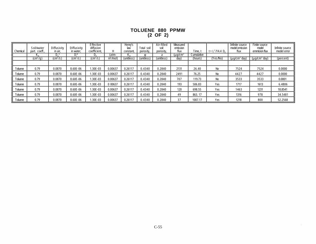
C-555 5
TOLUENE 880 PPMW(2 OF 2)
ChemicalSoil/water
part. coeff.,Diffusivity
in air,Diffusivityin water,
Effectivediffusion
coefficient, H
Henry’slaw
constant,Total soilporosity,
Air-fi l ledsoil
porosity,
Measuredemission
flux Time, t t > L 2 /14.4 DE
Infinite sourcemodel emission
flux
Finite sourcemodel
emmision fluxInfinite source
model errorKD Dg
a Diw DE (atm- KH φ a (µg/cm2- Cumulative
(cm3 / g ) (cm2 /s ) (cm2 /s ) (cm2 /s ) m3/mol) (unitless) (unitless) (unitless) day) (hours) (Yes/No) (µg/cm2- day) (µg/cm2- day) (percent)
Toluene 0.79 0.0870 8.60E-06 1.30E-03 0.00637 0.26117 0.4340 0.2840 2131 26.40 No 7524 7524 0.0000
Toluene 0.79 0.0870 8.60E-06 1.30E-03 0.00637 0.26117 0.4340 0.2840 2491 76.25 No 4427 4427 0.0000
Toluene 0.79 0.0870 8.60E-06 1.30E-03 0.00637 0.26117 0.4340 0.2840 707 119.73 No 3533 3533 0.0001
Toluene 0.79 0.0870 8.60E-06 1.30E-03 0 00637 0.26117 0.4340 0.2840 193 506.83 Yes 1717 1613 6.4806
Toluene 0.79 0.0870 8.60E-06 1.30E-03 0.00637 0.26117 0.4340 0.2840 120 698.55 Yes 1463 1231 18.8541
Toluene 0.79 0.0870 8.60E-06 1.30E-03 0.00637 0.26117 0.4340 0.2840 49 863. 17 Yes 1316 978 34.5481
Toluene 0.79 0.0870 8.60E-06 1.30E-03 0.00637 0.26117 0.4340 0.2840 37 1007.17 Yes 1218 800 52.2568

C-565 6
ETHYLBENZENE 310 PPMW(1 of 2)
ChemicalSamplePoint
Initial soilconc.
Initial soilconc.
Fluxchambersurface Soil Depth Soil Type
Soil bulkdensity,
Soilparticledensity,
Gravimetricsoil moisture,
Water-filled soilporosity, Solubility
Soilorganiccarbon,
Satura-tion conc., Co>Csat
Measuredemission
flux
Organiccarbonpart.
coeff.,Co Co area ( L ) ρb ρs w Θ S fo c Csat (µg/cm2 Koc
(mg/kg) (g /g ) (cm2 ) (cm) (g/cm3) (g/cm3) (wt. fraction) (unitless) (mg/L) (fraction) (mg/kg) (Yes/No) -min) (cm3 / g )
Ethylbenzene 3 310 3.1 0E-04 1300 91 Loamy Sand 1.5 2.65 0.10 0.1500 173 0.006 257 Yes 2640 221Ethylbenzene 4 310 3.1 0E-04 1300 91 Loamy Sand 1.5 2.65 0.10 0.1500 173 0.006 257 Yes 1700 221Ethylbenzene 5 310 3.1 0E-04 1300 91 Loamy Sand 1.5 2.65 0.10 0.1500 173 0.006 257 Yes 1080 221Ethylbenzene 6 310 3.1 0E-04 1300 91 Loamy Sand 1.5 2.65 0.10 0.1500 173 0.006 257 Yes 250 221Ethylbenzene 7 310 3.1 0E-04 1300 91 Loamy Sand 1.5 2.65 0.10 0.1500 173 0.006 257 Yes 180 221Ethyibenzene 8 310 3.1 0E-04 1300 91 Loamy Sand 1.5 2.65 0.10 0.1500 173 0.006 257 Yes 0 221

C-575 7
ETHYLBENZENE 310 PPMW(2 of 2)
ChemicalSoil/ waterpart. coeff.,
Diffusivityin air,
Diffusivityin water,
Effectivediffusion
coefficient,
Henry’slaw
constant,Total soilporosity,
Air-fi l ledsoil
porosity,Measured
emission fluxTime,
t t > L 2 /14.4 DE
Infinite sourcemodel emission
flux
Finite sourcemodel
emmision fluxInfinite source
model errorKD Dg
a Diw DE KH φ a (µg/cm2- Cumulative (µg/cm2- (µg/cm2-
(cm3 / g ) (cm2 /s ) (cm2 /s ) (cm2 /s ) (unitless) (unitless) (unitless) day) (hours) (Yes/No) day) day) (percent)
Ethylbenzene 1.33 0.0750 7.80E-06 8.64E-04 0.32021 0.4340 0.2840 380 26.40 No 2162 2162 0.0000
Ethylbenzene 1.33 0.0750 7.80E-06 8.64E-04 0.32021 0.4340 0.2840 245 76.25 No 1272 1272 0.0000
Ethylbenzene 1.33 0.0750 7.80E-06 8.64E-04 0.32021 0.4340 0.2840 156 119.73 No 1015 1015 0.0000
Ethylbenzene 1.33 0.0750 7.80E-06 8.64E-04 0.32021 0.4340 0.2840 36 506.83 Yes 493 488 1.0596
Ethylbenzene 1.33 0.0750 7.80E-06 8.64E-04 0.32021 0.4340 0.2840 26 698.55 Yes 420 402 4.6357
Ethyibenzene 1.33 0.0750 7.80E-06 8.64E-04 0.32021 0.4340 0.2840 0 863.17 Yes 373 343 10.0850
C-585 8
APPENDIX B
VALIDATION DATA FOR THE JURY REDUCED SOLUTION FINITESOURCE MODEL

C-595 9
TRIALLATE 10 PPM(1 OF 2)
ChemicalSamplePoint
Initialsoil conc.
Initial soilconc. Emitting
SoilDepth Soil Type
Soil bulkdensity,
Soilparticledensity,
Gravi-metric soilmoisture,
w
Water-filled soilporosity, Solubility
Soilorganiccarbon,
Saturationconc., Co>Csat
Measuredemission
flux
Organiccarbonpart.
coeff.,Co Co area ( L ) ρb ρs (wt. Θ S fo c Csat (µg/cm2 Koc
(mg/kg) (g /g ) (cm2 ) (cm) (Kg /L ) (Kg /L ) fraction) (unitless) (mg/L) (fraction) (mg/kg) (Yes/No) -day) (cm3 / g )
Triallate 1 10 1.00E-05 30 10 San Joaquin Sandy Loam 1.34 2.65 0.21 0.2787 4.00 0.0072 105 No 1.700 3600Triallate 2 10 1.00E-05 30 10 San Joaquin Sandy Loam 1.34 2.65 0.21 0.2787 4.00 0.0072 105 No 0.975 3600Triallate 3 10 1.00E-05 30 10 San Joaquin Sandy Loam 1.34 2.65 0.21 0.2787 4.00 0.0072 105 No 0.750 3600Triallate 4 10 1.00E-05 30 10 San Joaquin Sandy Loam 1.34 2.65 0.21 0.2787 4.00 0.0072 105 No 0.490 3600Triallate 5 10 1.00E-05 30 10 San Joaquin Sandy Loam 1.34 2.65 0.21 0.2787 4.00 0.0072 105 No 0.330 3600Triallate 6 10 1.00E-05 30 10 San Joaquin Sandy Loam 1.34 2.65 0.21 0.2787 4.00 0.0072 105 No 0.280 3600Triallate 7 10 1.00E-05 30 10 San Joaquin Sandy Loam 1.34 2.65 0.21 0.2787 4.00 0.0072 105 No 0.210 3600Triallate 8 10 1.00E-05 30 10 San Joaquin Sandy Loam 1.34 2.65 0.21 0.2787 4.00 0.0072 105 No 0.180 3600Triallate 9 10 1.00E-05 30 10 San Joaquin Sandy Loam 1.34 2.65 0.21 0.2787 4.00 0.0072 105 No 0.155 3600Triallate 10 10 1.00E-05 30 10 San Joaquin Sandy Loam 1.34 2.65 0.21 0.2787 4.00 0.0072 105 No 0.145 3600Triallate 11 10 1.00E-05 30 10 San Joaquin Sandy Loam 1.34 2.65 0.21 0.2787 4.00 0.0072 105 No 0.135 3600Triallate 12 10 1.00E-05 30 10 San Joaquin Sandy Loam 1.34 2.65 0.21 0.2787 4.00 0.0072 105 No 0.125 3600Triallate 13 10 1.00E-05 30 10 San Joaquin Sandy Loam 1.34 2.65 0.21 0.2787 4.00 0.0072 105 No 0.123 3600Triallate 14 10 1.00E-05 30 10 San Joaquin Sandy Loam 1.34 2.65 0.21 0.2787 4.00 0.0072 105 No 0.115 3600Triallate 15 10 1.00E-05 30 10 San Joaquin Sandy Loam 1.34 2.65 0.21 0.2787 4.00 0.0072 105 No 0.107 3600Triallate 16 10 1.00E-05 30 10 San Joaquin Sandy Loam 1.34 2.65 0.21 0.2787 4.00 0.0072 105 No 0.105 3600Triallate 17 10 1.00E-05 30 10 San Joaquin Sandy Loam 1.34 2.65 0.21 0.2787 4.00 0.0072 105 No 0.103 3600Triallate 18 10 1.00E-05 30 10 San Joaquin Sandy Loam 1.34 2.65 0.21 0.2787 4.00 0.0072 105 No 0.102 3600Triallate 19 10 1.00E-05 30 10 San Joaquin Sandy Loam 1.34 2.65 0.21 0.2787 4.00 0.0072 105 No 0.095 3600Triallate 20 10 1.00E-05 30 10 San Joaquin Sandy Loam 1.34 2.65 0.21 0.2787 4.00 0.0072 105 No 0.094 3600Triallate 21 10 1.00E-05 30 10 San Joaquin Sandy Loam 1.34 2.65 0.21 0.2787 4.00 0.0072 105 No 0.093 3600Triallate 22 10 1.00E-05 30 10 San Joaquin Sandy Loam 1.34 2.65 0.21 0.2787 4.00 0.0072 105 No 0.094 3600Triallate 23 10 1.00E-05 30 10 San Joaquin Sandy Loam 1.34 2.65 0.21 0.2787 4.00 0.0072 105 No 0.085 3600Triallate 24 10 1.00E-05 30 10 San Joaquin Sandy Loam 1.34 2.65 0.21 0.2787 4.00 0.0072 105 No 0.083 3600Triallate 25 10 1.00E-05 30 10 San Joaquin Sandy Loam 1.34 2.65 0.21 0.2787 4.00 0.0072 105 No 0.082 3600Triallate 26 1 0 1.00E-05 30 1 0 San Joaquin Sandy Loam 1.34 2.65 0.21 0.2787 4.00 0.0072 1 05 No 0.083 3600Triallate 27 10 1.00E-05 30 10 San Joaquin Sandy Loam 1.34 2.65 0.21 0.2787 4.00 0.00.72 105 No 0.080 3600Triallate 28 10 1.00E-05 30 10 San Joaquin Sandy Loam 1.34 2.65 0.21 0.2787 4.00 0.00.72 105 No 0.080 3600Trlallate 29 10 1.00E-05 30 10 San Joaquin Sandy Loam 1.34 2.65 0.21 0.2787 4.00 0.00.72 105 No 0.072 3600Triallate 30 10 1.00E-05 30 10 San Joaquin Sandy Loam 1.34 2.65 0.21 0.2787 4.00 0.0072 105 No 0 071 3600Triallate 31 10 1.00E-05 30 10 San Joaquin Sandy Loam 1.34 2.65 0.21 0.2787 4.00 0.0072 105 No 0 070 3600Triallate 32 10 1.00E-05 30 10 San Joaquin Sandy Loam 1.34 2.65 0.21 0.2787 4.00 0.0072 105 No 0.070 3600

C-606 0
TRIALLATE 10 PPM(2 OF 2)
ChemicalSoil/ waterpart. coeff.,
Diffusivity inair,
Diffusivity inwater,
Effectivediffusion
coefficient,Henry’s law
constant,Total soilporosity,
Air-filled soilporosity,
Measuredemission flux Time, t
Jury finitesource modelemission flux
KD Dga Di
w DE KH φ Cumulative(cm3 / g ) (cm2 /s ) (cm2 /s ) (cm2 /s ) (unitless) (unitless) (unitless) (µg/cm2- day) (hours) (µg/cm2- day)
Triallate 25.92 0.0450 5.00E-06 4.14E-08 0.00104 0.4943 0.2156 1.700 3 1.278Triallate 25.92 0.0450 5.00E-06 4.14E-08 0.00104 0.4943 0.2156 0.975 6 0.904Triallate 25.92 0.0450 5.00E-06 4.14E-08 0.00104 0.4943 0.2156 0.750 12 0.639Triallate 25.92 0.0450 5.00E-06 4.14E-08 0.00104 0.4943 0.2156 0.490 24 0.452Triallate 25.92 0.0450 5.00E-06 4.14E-08 0.00104 0.4943 0.2156 0.330 48 0.320Triallate 25.92 0.0450 5.00E-06 4.14E-08 0.00104 0.4943 0.2156 0.280 72 0.261Triallate 25.92 0.0450 5.00E-06 4.14E-08 0.00104 0.4943 0.2156 0.210 96 0.226Triallate 25.92 0.0450 5.00E-06 4.14E-08 0.00104 0.4943 0.2156 0.180 120 0.202Triallate 25.92 0.0450 5.00E-06 4.14E-08 0.00104 0.4943 0.2156 0.155 144 0.184Triallate 25.92 0.0450 5.00E-06 4.14E-08 0.00104 0.4943 0.2156 0.145 168 0.171Triallate 25.92 0.0450 5.00E-06 4.14E-08 0.00104 0.4943 0.2156 0.135 192 0.160Triallate 25.92 0.0450 5.00E-06 4.14E-08 0.00104 0.4943 0.2156 0.125 216 0.151Triallate 25.92 0.0450 5.00E-06 4.14E-08 0.00104 0.4943 0.2156 0.123 240 0.143Triallate 25.92 0.0450 5.00E-06 4.14E-08 0.00104 0.4943 0.2156 0.115 264 0.136Triallate 25.92 0.0450 5.00E-06 4.14E-08 0.00104 0.4943 0.2156 0.107 288 0.130Triallate 25.92 0.0450 5.00E-06 4.14E-08 0.00104 0.4943 0.2156 0.105 312 0.125Triallate 25.92 0.0450 5.00E-06 4.14E-08 0.00104 0.4943 0.2156 0.103 336 0.121Triallate 25.92 0.0450 5.00E-06 4.14E-08 0.00104 0.4943 0.2156 0.102 360 0.117Triallate 25.92 0.0450 5.00E-06 4.14E-08 0.00104 0.4943 0.2156 0.095 384 0.113Triallate 25.92 0.0450 5.00E-06 4.14E-08 0.00104 0.4943 0.2156 0.094 408 0.110Triallate 25.92 0.0450 5.00E-06 4.14E-08 0.00104 0.4943 0.2156 0.093 432 0.107Triallate 25.92 0.0450 5.00E-06 4.14E-08 0.00104 0.4943 0.2156 0.094 456 0.104Triallate 25.92 0.0450 5.00E-06 4.14E-08 0.00104 0.4943 0.2156 0.085 480 0.101Triallate 25.92 0.0450 5.00E-06 4.14E-08 0.00104 0.4943 0.2156 0.083 504 0.099Triallate 25.92 0.0450 5.00E-06 4.14E-08 0.00104 0.4943 0.2156 0.082 528 0.096Triallate 25.92 0.0450 5.00E-06 4.14E-08 0.00104 0.4943 0.2156 0.083 552 0.094Triallate 25.92 0.0450 5.00E-06 4.14E-08 0.00104 0.4943 0.2156 0.080 576 0.092Triallate 25.92 0.0450 5.00E-06 4.14E-08 0.00104 0.4943 0.2156 0.080 600 0.090Triailate 25.92 0.0450 5.00E-06 4.14E-08 0.00104 0.4943 0.2156 0.072 624 0.085Trialiate 25.92 0.0450 5.00E-06 4.14E-08 0.00104 0.4943 0.2156 0.071 648 0.087Triallate 25.92 0.0450 5.00E-06 4.14E-08 0.00104 0.4943 0.2156 0.070 672 0.085Triallate 25.92 0.0450 5.00E-06 4.14E-08 0.00104 0.4943 0.2156 0 070 696 0.084

APPENDIX D
Revisions to VF and PEF Equations (EQ, 1994b)

D-1
ENVIRONMENTAL QUALITY MANAGEMENT, INC.
MEMORANDUM
TO: Ms. Janine Dinan DATE: July 11, 1994
SUBJECT: Revisions to VF and PEF Equations FROM: Craig Mann
FILE: 5099-3 cc:
Subsequent to the evaluation of the dispersion equations in the RAGS - Part B performedby Environmental Quality Management, Inc. (EQ,1993), questions have arisen as to the accuracyof the modeling protocol used to derive the dispersion coefficient (Q/C) used in the volatilizationfactor (VF) and the particulate emission factor (PEF) presently employed to calculate the airpathway Soil Screening Levels (SSLs).
EQ, 1993 used the Industrial Source Complex model (ISC2-ST) to derive a normalizedconcentration (kg/m3 per g/m2-s) for a series of square and rectangular area sources of differingsize. This modeling protocol employed a source subdivision scheme similar to that recommendedin the ISC2-ST Model User's Manual (EPA, 1992) whereby the source was subdivided intosmaller sources closest to the center of the area. The center of the area was found to represent thepoint of maximum annual average concentration for all source shapes analyzed. Consecutive modelruns were performed whereby source subdivision was increased between runs. Final sourcesubdivision was reached when the model results converged within a factor of three percent or less.
From these data, a simple linear regression was used to evaluate the nature of therelationship between the normalized concentration and the size of the area. Preliminary plots of thedata indicated that the relationship was exponential. Therefore, the relationship was linearized bytaking the natural logarithms (ln) of each variable. The resulting linear regression for a square areaof 0.5 acres resulted in a normalized concentration (C/Q) of 0.0098 kg/m3 per g/m2-s; the inverseof the normalized concentration resulted in a dispersion coefficient (Q/C) of 101.8 g/m2-s perkg/m3.
On May 5, 1994 a teleconference was held between representatives of the ToxicsIntegration Branch of the Office of Emergency and Remedial Response (OERR) and the SourceReceptor Analysis Branch of the Office of Air Quality Planning Standards (OAQPS) to discuss therelative merits of the available area source algorithms as applied to nearfield and on-site receptorsexposed to ground-level nonbuoyant emissions. The conclusions drawn from this teleconferencewere that a new algorithm recently developed by OAQPS would yield more accurate results for theexposure scenario in question.
The new algorithm is incorporated into the ISC2 model platform in both short-term mode(AREA-ST) and long-term mode (AREA-LT). Both models employ a double numerical integrationover the area source in the upwind and crosswind directions as follows:
χπ σ σ σ
= Q K
2 u
VD
exp -0.5
Y dxA
s y z yx y dy∫ ∫
2
(1)
where QA = Area source emission rate (g/m2-s)
K = Units scaling coefficient

D-2
V = Vertical term
D = Decay term.
The integral in the lateral (i.e., crosswind or y) direction is solved analytically as:
y dy∫
exp -0.5
Y = erfc
Y
y yσ σ
2
(2)
where erfc is the complementary error function.
The integral in the longitudinal (i.e., upwind or x) direction is solved by using a weightedaverage of successive estimates of the integral using a trapezoidal approximation. The model usesthree separate criteria to determine convergence of the upwind integral. The result of thesenumerical methods is an estimate of the full integral that is essentially equivalent to, but much moreefficient than, the method of estimating the integral as a series of line sources, such as the methodused by the Point, Area, Line (PAL 2.0) model. Wind tunnel tests have also shown that the newalgorithm performs well with on-site and near-field receptors.
Because the new algorithm provides better concentration estimates and does not requiresource subdivision, a revised dispersion analysis was performed for both volatile and particulatematter contaminants using the new algorithm.
The first part of the analysis involved a determination of the relationship betweenconcentration and source size. In addition, this part of the analysis included a determination of thepoint of maximum annual average concentration for a square area source. This assessmentemployed the AREA-ST model as acquired from the OAQPS Technology Transfer Network,Support Center for Regulatory Air Models (SCRAM) Bulletin Board.
Meteorological data used for this analysis were 1989 hourly data for the Los AngelesNational Weather Service (NWS) surface station, upper air data were from the Oakland NWSstation for the same year. Rural dispersion coefficients were employed and all regulatory defaultoptions used. Modeling assumed flat terrain with no flagpole receptors; source rotation angle wasset equal to zero.
Five source sizes were included in the assessment: 0.5, 5, 30, 200, and 600 acres. Acoarse Cartesian receptor grid was employed within and extending beyond the source perimeter; adiscrete receptor was also placed at the center of each source (x,y = 0,0). Emissions from eachsource were set equal to 1.0 g/m2-s; concentrations were calculated in units of kg/m3.
Figure 1 shows the relationship between source size (acres) and annual averageconcentration (kg/m3) for the five source sizes modeled. In each case, the point of maximumconcentration was located at the center of the source. As an example, Attachment A is the modelrun sheets for the 0.5 acre source. As can be seen from Figure 1, the relationship betweenconcentration and source size is exponential. Results also show that the maximum concentrationrepresenting the 600 acre source is 2.9 times higher than that of the 0.5 acre source.
Having established that when using the AREA-ST model the point of maximumconcentration for a square area source is the center receptor, the second part of the analysis was todetermine which of the 29 meteorological sites from EQ, 1993 best represents the averageexposure and the high end exposure to volatile and particulate matter emissions. It was determinedthat the average exposure case should be represented by the 50th percentile site concentration,while the high end exposure is best represented by the 90th percentile site concentration.

D-3
Figure 1Normalized Annual Average Concentration Versus Source Size

D-4
Each of the 29 sites from EQ, 1993 were subsequently modeled at an emission rate of 1.0g/m2-s with a single discrete receptor at the center of the square area source. Source sizes modeledwere 0.5 acres and 30 acres. Hourly meteorological data for each site were from EQ, 1993. Fromthe set of SS normalized annual average concentrations, the 50th percentile site was determined tobe Salt Lake City, Utah; Los Angeles, California (89th percentile site) was determined to be theclosest approximation of the 90th percentile site. Table 1 shows the resulting dispersioncoefficients for the two source sizes and the percentile ranking of each site.
In order to determine the average and high end sites for particulate matter exposuresresulting from wind erosion, a normalized concentration could not be used because meteorologicalconditions other than simple dispersion (i.e., wind velocity and frequency) influence emissionsand therefore actual concentrations. For this reason, actual concentrations were calculated for eachsite using the existing PEF equation as follows:
C = (C/Q) 0.036 (1- V) x (U /U ) x F(x)
3600 s/hm t-7
3
(3)
where C = Annual average PM10 concentration, kg/m3
(C/Q) = Normalized annual average concentration (kg/m3 per g/m2 -s)
V = Fraction of continuous vegetative cover
Um = Mean annual windspeed, m/s
Ut-7 = Equivalent threshold value of windspeed at 7 m, m/s
F(x) = Windspeed distribution function from Cowherd, 1985.
The value of (C/Q) for each site was the normalized concentration previously estimated forvolatile emissions (i.e., the inverse of each dispersion coefficient in Table 1). The value of V wasset equal to 0.5. The mean annual windspeed (Um) for each site was taken from Weather of U.S.Cities, Second Edition, Volume 2 by J. A. Ruffner and F. E. Bair, Gale Research Co., Detroit,Michigan. The value of F(x) was estimated for each site from Figure 4-3 or calculated fromAppendix B of Cowherd 1985, as appropriate.
The value of Ut-7 was calculated as follows:
Ut−
7 =
U
0.4 ln
700
zt
0
(4)
where Ut-7 = Equivalent threshold value of windspeed at 7 m, m/s
Zo = Surface roughness height, cm (zo = 0.5 cm for open terrain)
Ut = Threshold friction velocity, m/s (Ut = 0.625 m/s).
Table 2 gives the results of this analysis and shows the relative PM10 concentrations foreach site by source size and the percentile rankings. As can be seen from Table 2, the 50thpercentile site was Salt Lake City, Utah, while the 89th percentile site was Minneapolis,Minnesota.

D-5
TABLE 1.VOLATILE DISPERSION SITE RANKINGS
City
NWSSurfaceStationNumber
0.5 Acre(Q /C )
(g/m2-s perkg/m3)
30 Acre(Q /C )
(g/m2-s perkg/m3)
S i teRanking
Percenti le( % )
Huntington 13860 52.77 27.08 100Fresno 93193 62.00 31.85 96Phoenix 23183 64.06 32.63 93Los Angeles 2 4 1 7 4 6 8 . 8 2 3 5 . 1 0 8 9Winnemucca 24128 69.25 35.49 86Boise 24131 69.40 35.69 82Hartford 14740 71.33 36.64 79Little Rock 13963 73.37 37.68 75Portland 14764 74.24 37.86 71Salem 24232 73.42 37.88 68Charleston 13880 74.91 38.42 64Denver 23062 75.59 38.80 61Atlanta 13874 77.16 39.68 57Raleigh-Durham 13722 77.46 39.87 54Salt Lake City 2 4 1 2 7 7 8 . 0 6 4 0 . 1 4 5 0Houston 12960 79.24 40.70 46Lincoln 14939 81.63 41.56 43Harrisburg 14751 81.90 42.34 39Bismarck 24011 83.40 42.72 36Seattle 24233 82.71 42.81 32Cleveland 14820 83.19 43.03 29Albuquerque 23050 84.18 43.31 25Miami 12839 85.40 43.57 21San Francisco 23234 89.53 46.06 18Philadelphia 13739 90.09 46.38 14Minneapolis 14922 90.74 46.84 11Las Vegas 23169 95.51 49.48 7Chicago 94846 97.75 50.45 4Casper 24089 100.00 51.68 0

D-6
TABLE 2. PEF.CALCULATIONS AND SITE RANKINGS
NWSsurfacestation
Meanannualwind-speed
Meanannualwind-speed
Roughnessheight, Zo t
Thresholdfriction
velocity atsurface
Thresholdfriction
velocity at7 m
F(x), F(x), Vegetativecover
PM10emission
flux
0.5 Acre(Q/C)
(g/m2-sper
0.5 Acreannual
averageconc.
30 Acre(Q/C)
(g/m2-sper
30 Acreannual
averageconc.
Siteranking
percentile
City number (mph) (m/s) (cm) (m/s) (m/s) x x <= 2 x > 2 (fraction) (g/m2-s) kg/m3) (ug/m3) kg/ m3) (ug/ m3) (%)
Casper 24089 12.9 5.77 0.5 0.625 11.32 1.74 0.57 NA 0.50 3.77E-07 100.00 3.77 51.68 7.29 100Cleveland 14820 10.8 4.83 0.5 0.625 11.32 2.08 NA 2.32E-01 0.50 9.01E-08 83.19 1.08 43.03 2.09 96Lincoln 14939 10.4 4.65 0.5. 0.625 11.32 2.16 NA 1.82E-01 0.50 6.30E-08 81.63 077 41.56 1.52 93Minneapolis 14922 10.5 4.69 0.5 0.625 11.32 2.14 NA 1.94E-01 0.50 6.92E-08 90.74 0.76 46.84 1.48 89Bismarck 24011 10.3 4.60 0.5 0.625 11.3Z 2.18 NA 1.70E-01 0.50 5.73E-08 83.40 0.69 42.72 1.34 86Chicago 94846 10.4 4.65 0.5 0.625 11.32 2.16 NA 1.82E-01 0.50 6.30E-08 97.75 0.64 50.45 1.25 82Philadelphia 13739 9.6 4.29 0.5 0.625 11.32 2.34 NA 9.93E-02 0.50 2.71E-08 90.09 0.30 46.38 0.58 79Miami 12835 9.2 4.11 0.5 0.625 11.32 2.44 NA 6.82E-02 0.50 1.64E-08 85.40 0.19 43.57 0.38 75Altanta 13874 9.1 4.07 0.5 0.625 11.32 2.47 NA 6.16E-02 0.50 1.43E-08 77.16 0.19 39.68 0.36 71Seattle 24233 9.1 4.07 0.5 0.625 11.32 2.47 NA 6.16E-02 0.50 1.43E-08 82.71 0.17 42.81 0.33 68Boise 24131 8.9 3.98 0.5 0.625 11.32 2.52 NA 4.95E-02 0.50 1.07E-08 69.40 0.15 35.69 0.30 64Las Vegas 23165 9.1 4.07 0.5 0.625 11.32 2.47 NA 6.16E-02 0.50 1.43E-08 95.51 0.15 49.48 0.29 61Albuquerque 23050 9.0 4.02 0.5 0.625 11.32 2.49 NA 5.53E-02 0.50 1.24E-08 84.18 0.15 43.31 0.29 57Denver 23062 8.8 3.93 0.5 0.625 11.32 2.55 NA 4.41E-02 0.50 9.25E-09 75.59 0.12 38.80 0.24 54Salt Lake City 24127 8.8 3.93 0.5 0.625 11.32 2.55 NA 4.41E-02 0.50 9.25E-09 78.06 0.12 40.14 0.23 50Portland 14762 8.7 3.89 0.5 0.625 11.32 2.58 NA 3.91E-02 0.50 7.93E-09 74.24 0.11 37.86 0.21 46Charleston 13880 8.7 3.89 0.5 0.625 11.32 2.58 NA 3.91E-02 0.50 7.93E-09 74.91 0.11 38.42 0.21 43Hartford 14764 8.6 3.84 0.5 0.625 11.32 2.61 NA 3.45E-02 0.50 6.76E-09 71.33 0.095 36.64 0.18 39San Francisco 23234 8.7 3.89 0.5 0.625 11.32 2.58 NA 3.91E-02 0.50 7.93E-09 89.53 0.089 46.06 0.17 36Little Rock 13963 8.0 3.58 0.5 0.625 11.32 2.80 NA 1.45E-02 0.50 2.29E-09 73.37 0.031 37.68 0.061 32Winnemucca 24128 7.9 3.53 0.5 0.625 11.32 2.84 NA 1.23E-02 0.50 1.86E-09 69.25 0.027 35.49 0.052 29Houston 12960 7.8 3.49 0.5 0.625 11.32 2.88 NA 1.03E-02 0.50 1.51E-09 79.24 0.019 40.70 0.037 25Raleigh-Durham
13722 7.7 3.44 0.5 0.625 11.32 2.91 NA 8.60E-03 0.50 1.21E-09 77.461 0.016 39.87 0.030 21
Harrisburg 14751 7.7 3.44 0.5 0.625 11.32 2.91 NA 8.60E-03 0.50 1.21E-09 81.90 0.015 42.34 0.029 18LosAngeles 24174 7.4 3.31 0.5 0.625 11.32 3.03 NA 4.74E-03 0.50 5.92E-10 68.82 8.60E-03 35.10 0.017 14Salem 2423 2 7.0 3.13 0.5 0.625 11.32 3.21 NA 1.87E-03 0.50 1.98E-10 73.42 2.69E-03 37.88 5.22E-03 11Huntington 13860 6.5 2.91 0.5 0.625 11.32 3.45 NA 4.45E-04 0.50 3.76E-11 52.77 7.13E-04 27.08 1.39E-03 7Fresno 93193 6.4 2.86 0.5 0.625 11.32 3.51 NA 3.19E-04 0.50 2.58E-11 62.00 4.16E-04 31.85 8.09E-04 4Phoenix 23183 6.3 2.82 0.5 0.625 11.32 3.56 NA 2.25E-04 0.50 1.73E-11 64.06 2.71E-04 32.63 5.31E-04 0
F(x) <= 2 from Cowherd (1985), Figure 4-3.F(x) > 2 from Cowherd (1985), Appendix B.NA = Not Appilcable.r
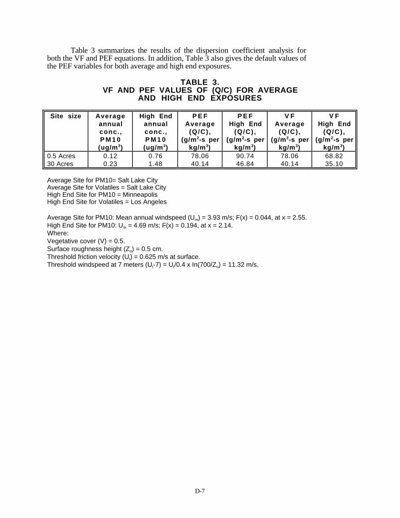
D-7
Table 3 summarizes the results of the dispersion coefficient analysis forboth the VF and PEF equations. In addition, Table 3 also gives the default values ofthe PEF variables for both average and high end exposures.
TABLE 3.VF AND PEF VALUES OF (Q/C) FOR AVERAGE
AND HIGH END EXPOSURES
Site size Averageannualconc.,P M 1 0
(ug/m3)
High Endannualconc.,P M 1 0
(ug/m3)
P E FAverage
(Q/C) ,(g/m2-s per
kg/m3)
P E FHigh End
(Q/C) ,(g/m2-s per
kg/m3)
V FAverage
(Q/C) ,(g/m2-s per
kg/m3)
V FHigh End
(Q/C) ,(g/m2-s per
kg/m3)0.5 Acres30 Acres
0.120.23
0.761.48
78.0640.14
90.7446.84
78.0640.14
68.8235.10
Average Site for PM10= Salt Lake CityAverage Site for Volatiles = Salt Lake CityHigh End Site for PM10 = MinneapolisHigh End Site for Volatiles = Los Angeles
Average Site for PM10: Mean annual windspeed (Um) = 3.93 m/s; F(x) = 0.044, at x = 2.55.High End Site for PM10: Um = 4.69 m/s; F(x) = 0.194, at x = 2.14.Where:Vegetative cover (V) = 0.5.Surface roughness height (Zo) = 0.5 cm.Threshold friction velocity (Ut) = 0.625 m/s at surface.Threshold windspeed at 7 meters (Ut-7) = Ut/0.4 x In(700/Zo) = 11.32 m/s.

D-8
ATTACHMENT A
AREA-ST MODEL RUN SHEETS FOR A 0.5 ACRE SQUARE AREA SOURCE
CO STARTINGCO TITLEONE AREA SOURCES--- 1/2 acre runCO MODELOPT DFAULT CONC RURALCO AVERTIME PERIODCO POLLUTID PM10CO RUNORNOT RUNCO ERRORFIL AREA1.ERRCO FINISHED
SO STARTINGSRCID SRCTYP XS YS ZS
SO LOCATION A1/2 AREA -22.5 -22.5 .0000SRCID QS HS XINIT YINIT
SO SRCPARAH A1/2 1.0 0.0 45. 45.
SO EHISUNIT .100000E-02 (GRAMS/(SEC-M**2)) KILOGRAMS/CUBIC-METER
SO SRCGROUP AREA1 A1/2
SO FINISHED
RE STARTINGRE DISCCART 0. o.RE DISCCART 25. 0.RE DISCCART -25. o.RE DISCCART 25. 25.RE DISCCART 25. -25.RE DISCCART -25. -25.RE DISCCART -25. 25.RE DISCCART 50. 0.RE DISCCART -50. 0.RE DISCCART 50. 50.RE DISCCART 50. -50.RE DISCCART -50. -50.RE DISCCART -50. 50.RE DSSCCART 75. 0.RE DISCCART -75. 0.RE DISCCART 75. 75.RE DISCCART 75. -75.RE DISCCART -75. -75.RE DISCCART -75. 75.RE DISCCART 100. 0.RE DISCCART -100. 0.RE DISCCART 100. 100.RE DISCCART 100. -100.RE DISCCART -100. -100.RE DISCCART -100. 100.
RE FINISHED
ME STARTINGME INPUTFIL C:\CRAIG\23174-89.ASCME ANEHHGHT 10.0 METERSME SURFDATA 23174 1989 LOS ANGELESME UAIRDATA 23230 1989 OAKLAND

D-9
ME WINDCATS 1.54 3.09 5.14 8.23 10.80ME FINISHED
OU STARTINGOU RECTABLE ALLAVE FIRSTOU FINISHED
****************************************************** SETUP Finishes Successfully ******************************************************

D-10
*** AREAST - VERSION TESTA *** *** AREA SOURCES---1/2 acre run***TEST OF ST AREA SOURCE ALGORITHM *** ***
*** MODELING OPTIONS USED: CONC RURAL FLAT DFAULT
*** MODEL SETUP OPTIONS SUMMARY ***
**Model Is Setup For Calculation of Average CONCentration Values.
**Model Uses RURAL Dispersion.
**Model Uses Regulatory DEFAULT Options:1. Final Plume Rise.2. Stack-tip Downwash.3. Buoyancy-induced Dispersion.4. Use Calms Processing Routine.5. Not Use Missing Data Processing Routine.6. Default Wind Profile Exponents.7. Default Vertical Potential Temperature Gradients.8. “Upper Bound” Values for Supersquat Buildings.9. No Exponential Decay for RURAL Mode
**Model Assumes Receptors on FLAT Terrain.
**Model Assumes No FLAGPOLE Receptor Heights.
**Model Calculates PERIOD Averages Only
**This Run Includes: 1 Source(s); 1 Source Group(s); and 25 Receptore(s)
**The Model Assumes A Pollutant Type of: PM10
**Model Set To Continue RUNning After the Setup Testing.ff
**Output Options Selected:Model Outputs Tables of PERIOD Averages by ReceptorModel Outputs Tables of Highest Short Term Values by Receptor (RECTABLE Keyword)
**NOTE: The Following Flags May Appear Following CONC Values:c for Calm Hoursm for Hissing Hoursb for Both Calm and Missing Hours
**Misc. Inputs:Anem. Hgt. (m) = 10.00 ; Decay Coef. =.0000 ; Rot. Angle = .0Emission Units = (GRAMS/(SEC-M**2)); Emission Rate Unit Factor = .lOOOOE-02Output Units = KILOGRAMS/CUBIC-METER
**input Runstream File: area1.dat, **Output Print File: area1.out**Detailed Error/Message File: AREA1.ERR

D-11
*** AREAST - VERSION TESTA *** *** AREA SOURCES--- 1/2 acre run ***TEST OF ST AREA SOURCE ALGORITHM *** ***
*** MODELING OPTIONS USED: CONC RURAL FLAT DFAULT
*** AREA SOURCE DATA ***
SOURCEID
NUMBERPART.CATS.
EMISSION RATE(USER UNITS/METERS**2)
COORDX(METERS)
(SW CORNER)Y(METERS)
BASEELEV.(METERS)
RELEASEHEIGHT(METERS)
X-DIM OFAREA(METERS)
Y-DIM OFAREA(METERS)
ORIENT.OF AREA(DEG.)
EMISSIONRATE SCALARVARY BY
A1/2 0 .10000E+01 -22.5 -22.5 .0 .00 45.00 45.00 .00
*** AREAST - VERSION TESTA *** *** AREA SOURCES--- 1/2 acre run ***TEST OF ST AREA SOURCE ALGORITHM *** ***
*** MODELING OPTIONS USED: CONC RURAL FLAT DFAULT
*** SOURCE IDs DEFINING SOURCE GROUPS ***
GROUP ID SOURCE IDs
AREA1 A1/2

D-12
*** AREAST - VERSION TESTA *** *** AREA SOURCES--- 1/2 acre runTEST OF ST AREA SOURCE ALGORITHM *** ***
*** MODELING OPTIONS USED: CONC RURAL FLAT DFAULT
*** DISCRETE CARTESIAN RECEPTORS ***(X-COORD, Y-C00RD, ZELEV, ZFLAG) (METERS)
( .0, .0, .0, .0); ( 25.0, .0, .0, .0);( -25.0, .0, .0, .0); ( 25.0, 25.0, .0, .0);( 25.0 -25.0, .0, .0); ( -25.0, -25.0, .0, .0);( -25.0 25.0, .0, .0); ( 50.0, .0, .0, .0);( -50.0, .0, .0, .0); ( 50.0, 50.0, .0, .0);( 50.0 -50.0, .0, .0); ( -50.0, -50.0, .0, .0);( -50.0 50.0, .0, .0); ( 75.0, .0, .0, .0);( -75.0, .0, .0, .0); ( 75.0, 75.0, .0, .0);( 75.0, -75.0, .0, .0); ( -75.0, -75.0, .0, .0);( -75.0, 75.0, .0, .0); ( 100.0, .0, .0, .0);( -100.0, .0, .0, .0); ( 100.0, 100.0, .0, .0);( 100.0, 100.0, .0, .0); ( -100.0, -100.0, .0, .0);( -100.0, 100.0, .0, .0);
.,

D-13
*** AREAST - VERSION TESTA *** *** AREA SOURCES--- 1/2 acre runTEST OF ST AREA SOURCE ALGORITHM *** ***
*** MODELING OPTIONS USED CONC RURAL FLAT DFAULT
*** METEOROLOGICAL DAYS SELECTED FOR PROCESSING ***(1=YES; 0=NO)
1111111111 1111111111 1111111111 1111111111 11111111111111111111 1111111111 1111111111 1111111111 11111111111111111111 1111111111 1111111111 1111111111 11111111111111111111 1111111111 1111111111 1111111111 11111111111111111111 1111111111 1111111111 1111111111 11111111111111111111 1111111111 1111111111 1111111111 11111111111111111111 111111
NOTE: METEOROLOGICAL DATA ACTUALLY PROCESSED WlLL ALSO DEPEND ON WHAT IS INCLUDED IN THE DATA FILE
*** UPPER BOUND OF FIRST THROUGH FIFTH WIND SPEED CATEGORIES ***(HETERS/SEC)
1.54, 3.09, 5.14, 8.23, 10.80,
*** WIND PROFILE EXPONENTS ***
STABILITY WlND SPEED CATEGORYCATEGORY 1 2 3 4 5 6
A .70000E-01 .70000E-01 .70000E-01 .70000E-01 .70000E-01 .70000E-01B .70000E-01 .70000E-01 .70000E-01 .70000E-01 .70000E-01 .70000E-01C .10000E+00 .10000E+00 .10000E+00 .10000E+00 .10000E+00 .10000E+00D .15000E+00 .15000E+00 .15000E+00 .15000E+00 .15000E+00 .15000E+00E .35000E+00 .35000E+00 .35000E+00 .35000E+00 .35000E+00 .35000E+00F .55000E+00 .55000E+00 .55000E+00 .55000E+00 .55000E+00 .55000E+00
*** VERTICAL POTENTIAL TEMPERATURE GRADIENTS ***(DEGREES KELVIN PER METER)
STABILITY WIND SPEED CATEGORYCATEGORY 1 2 3 4 5 6
A .00000E+00 .O0000E+00 .00000E+00 .00000E+00 .00000E+00 .O0000E+00B .00000E+00 .00000E+00 .00000t+00 .00000E+00 .00000E+OO .00000E+OOC .00000E+00 .00000E+00 .00000E+00 .00000E+00 .00000E+00 .00000E+00D .00000E+00 .00000E+00 .00000E+00 .00000E+00 .00000E+00 .OO000E+00E .20000E-01 .20000E-01 .20000E-01 .20000E-01 .20000E-01 .20000E-01F .35000E-01 .35000E-01 .35000E-01 .35000E-01 .35000E-01 .35000E-01

D-14
*** AREAST - VERSION TESTA *** *** AREA SOURCES--- 1/2 acre run ***TEST OF ST AREA SOURCE ALGORITHM *** ***
*** MODELING OPTIONS USED: CONC RURAL FLAT DFAULT
*** THE FIRST 24 HOURS OF METEOROLOGICAL DATA ***
FILE: C:\CRAIG\23174-89.ASC FORMAT: (412,2F9.4,F6.1,I2,2F7.1)SURFACE STATION NO : 23174 UPPER AIR STATION NO.: 23230NAME: LOS NAME: OAKLANDYEAR: 1989 YEAR: 1989
YEAR MONTH DAY HOUR FLOWVECTOR
SPEED(M/S)
TEMP(K)
STABCLASS
MIXINGRURAL
HEIGHT (M)URBAN
89 1 1 1 251.0 3.09 282.6 4 533.0 533.089 1 1 2 228.0 3.09 282.0 4 568.6 568.689 1 1 3 194.0 2.57 282.0 4 604.1 604.189 1 1 4 143.0 4.63 282.0 4 639.6 639.689 1 1 5 173.0 2.06 282.0 5 675.2 151.089 1 1 6 272.0 3.09 280.4 6 710.7 151.089 1 1 7 265.0 2.06 280.4 6 746.3 151.089 1 1 8 233.0 2.06 282.0 5 134.9 265.489 1 1 9 257.0 2.06 283.7 4 278.2 387.089 1 1 10 261.0 .00 285.9 3 421.6 508.689 1 1 11 44.0 2.06 288.2 3 564.9 630.289 1 1 12 56.0 3.60 289.3 3 708.3 751.889 1 1 13 83.0 4.12 289.3 3 851.6 873.489 1 1 14 59.0 4.12 290.4 3 995.0 995.089 1 1 15 82.0 4.12 287.6 3 995.0 995.089 1 1 16 74.0 3.60 287.6 4 995.0 995.089 1 1 17 81.0 3.60 285.9 5 992.3 979.189 1 1 18 87.0 3.09 284.3 6 975.8 880.689 1 1 19 154.0 4.12 286.5 5 959.2 782.289 1 1 20 167.0 2.06 285.4 6 942.7 683.889 1 1 21 280.0 2.57 285.4 6 926.2 585.389 1 1 22 252.0 2.06 284.3 6 909.6 486.989 1 1 23 220.0 3.09 283.2 6 893.1 388.489 1 1 24 260.0 1.54 283.7 7 876.5 290.0
*** NOTES: STABILITY CLASS 1=A, 2=B, 3=C, 4=D, 5=E AND 6=F. FLOW VECTOR IS DIRECTION TOWARD WHICH WIND IS BLOWING.

D-15
*** AREAST - VERSION TESTA *** *** AREA SOURCES--- 1/2 acre run ***TEST OF ST AREA SOURCE ALGORITHM *** ***
*** MODELING OPTIONS USED: CONC RURAL FLAT DFAULT
*** THE PERIOD ( 8760 HRS) AVERAGE CONCENTRATION VALUES FOR SOURCE GROUP: AREA1 ***INCLUDING SOURCE(S): A1/2,
*** DISCRETE CARTESIAN RECEPTOR POINTS ***
** CONC OF PM10 IN KILOGRAMS/CUBIC-METER **
X-COORD (M) Y-COORD (M) CONE X-COORD (M)) Y-COORD (M CONC
.00 .00 .01453 25.00 .00 .00679-25.00 .00 .00594 25.00 25.00 .0041425.00 -25.00 .00104 -25.00 -25.00 .00220-25.00 25.00 .00223 50.00 .00 .00175-50.00 .00 .00158 50.00 50.00 .0006050.00 -50.00 .00018 -50.00 -50.00 .00034-50.00 50.00 .00037 75.00 .00 .00076-75.00 .00 .00078 75.00 75 .00 .0002475.00 -75.00 .00008 -75.00 -75.00 .00015-75.00 75.00 .00016 100.00 .00 .00041-100.00 .00 .00047 100.00 100.00 .00013100.00 -100.00 .00005 -100.00 -100.00 .00009-100.00 100.00 .00009

D-16
*** AREAST - VERSION TESTA *** *** AREA SOURCES--- 1/2 acre runTEST OF ST AREA SOURCE ALGORITHM ***
*** MODELING OPTIONS USED: CONC RURAL FLAT DFAULT
*** THE SUMMARY OF MAXIMUM PERIOD ( 8760 HRS) RESULTS ***
** CONC OF PM10IN KILOGRAMS/CUBIC-METER **
NETWORKGROUP ID AVERAGE CONC RECEPTOR (XR, YR, ZELEV, ZFLAG) OF TYPE GRID-ID
AREA1 1ST HIGHEST VALUE IS .01453 AT ( .00, .00, .00, .00) DC2ND HIGHEST VALUE IS .00679 AT ( 25.00, .00, .00, .00) DC3RD HIGHEST VALUE IS .00594 AT ( -25.00, .00, .00, .00) DC4TH HIGHEST VALUE IS .00414 AT ( 25.00, 25.00, .00, .00) DC5TH HIGHEST VALUE IS .00223 AT ( -25.00, 25.00, .00, .00) DC6TH HIGHEST VALUE IS .00220 AT ( -25.00, -25.00, .00, .00) DC
*** RECEPTOR TYPES:GC = GRIDCARTGP = GRIDPOLRDC = DISCCARTDP = DISCPOLRBD = BOUNDARY

D-17
*** AREAST - VERSION TESTA *** *** AREA SOURCES--- 1/2 acre run ***TEST OF ST AREA SOURCE ALGORITHM *** ***
*** MODELING OPTIONS USED: CONC RURAL FLAT DFAULT
*** Message Summary For ISC2 Model Execution ***
-------- Summary of Total Messages --------
A Total of 0 Fatal Error Message(s)A Total of 0 Warning Message(s)A Totat of 653 Informational Message(s)
A Total of 653 Calm Hours Identified
******** FATAL ERROR MESSAGES *********** NONE ***
******** WARNING MESSAGES *********** NONE ***
*********************************************** ISCST2 Finishes Successfully ***********************************************

APPENDIX E
Determination of Ground Water Dilution AttenuationFactors

DETERMINATION OF GROUNDWATERDILUTION ATTENUATION FACTORS
FOR FIXED WASTE SITE AREASUSING EPACMTP
BACKGROUND DOCUMENT
EPA OFFICE OF SOLID WASTE
May 11, 1994

TABLE OF CONTENTS
Page
PREFACE ... . . . . . . . . . . . . . . . . . . . . . . . . . . . . . . . . . . . . . . . . . . . . . . . . . . . . . . . . . . . . . . . . . . . . . . . . . . . . . . . . . . . . . . . . . . . . . . . . . i
ABSTRACT... . . . . . . . . . . . . . . . . . . . . . . . . . . . . . . . . . . . . . . . . . . . . . . . . . . . . . . . . . . . . . . . . . . . . . . . . . . . . . . . . . . . . . . . . . . . . . . ii
1.0 INTRODUCTION... . . . . . . . . . . . . . . . . . . . . . . . . . . . . . . . . . . . . . . . . . . . . . . . . . . . . . . . . . . . . . . . . . . . . . . . . . . . .E-1
2.0 GROUNDWATER MODEL .. . . . . . . . . . . . . . . . . . . . . . . . . . . . . . . . . . . . . . . . . . . . . . . . . . . . . . . . . . . . . . . . . .E-2
2.1 Description of EPACMTP Model.. . . . . . . . . . . . . . . . . . . . . . . . . . . . . . . . . . . . . . . . . . . . . . . . . . . .E-2
2.2 Fate and Transport Simulation Modules . . . . . . . . . . . . . . . . . . . . . . . . . . . . . . . . . . . . . . . . . . . . .E-2
2.2.1 Unsaturated zone flow and transport module . . . . . . . . . . . . . . . . . . . . . . . . . . . . . .E-22.2.2 Saturated zone flow and transport module . . . . . . . . . . . . . . . . . . . . . . . . . . . . . . . . .E-42.2.3 Model capabilities and limitations.. . . . . . . . . . . . . . . . . . . . . . . . . . . . . . . . . . . . . . . . . . .E-5
2.3 Monte Carlo Module.. . . . . . . . . . . . . . . . . . . . . . . . . . . . . . . . . . . . . . . . . . . . . . . . . . . . . . . . . . . . . . . . . . .E-7
2.3.1 Capabilities and Limitations of Monte Carlo Module. . . . . . . . . . . . . . . . . . . . E-10
3.0 MODELING PROCEDURE ... . . . . . . . . . . . . . . . . . . . . . . . . . . . . . . . . . . . . . . . . . . . . . . . . . . . . . . . . . . . . . . E-11
3.1 Modeling Approach.. . . . . . . . . . . . . . . . . . . . . . . . . . . . . . . . . . . . . . . . . . . . . . . . . . . . . . . . . . . . . . . . . . E-11
3.1.1 Determination of Monte Carlo Repetition Number andSensitivity Analysis . . . . . . . . . . . . . . . . . . . . . . . . . . . . . . . . . . . . . . . . . . . . . . . . . . . . . . . . . E-11
3.1.2 Analysis of DAF Values for Different Source Areas . . . . . . . . . . . . . . . . . . . . E-123.1.2.1 Model Options and Input Parameters . . . . . . . . . . . . . . . . . . . . . . . . E-13
4.0 RESULTS ... . . . . . . . . . . . . . . . . . . . . . . . . . . . . . . . . . . . . . . . . . . . . . . . . . . . . . . . . . . . . . . . . . . . . . . . . . . . . . . . . . . . E-18
4.1 Convergence of Monte Carlo Simulation .. . . . . . . . . . . . . . . . . . . . . . . . . . . . . . . . . . . . . . . . . E-184.2 Parameter Sensitivity Analysis . . . . . . . . . . . . . . . . . . . . . . . . . . . . . . . . . . . . . . . . . . . . . . . . . . . . . . E-184.3 DAF Values as a Function of Source Area.. . . . . . . . . . . . . . . . . . . . . . . . . . . . . . . . . . . . . . . . E-21
REFERENCES ... . . . . . . . . . . . . . . . . . . . . . . . . . . . . . . . . . . . . . . . . . . . . . . . . . . . . . . . . . . . . . . . . . . . . . . . . . . . . . . . . . . . . . . E-29

LIST OF FIGURES
Page
Figure 1 Conceptual view of the unsaturated zone-saturated zonesystem simulatedby EPACMTP... . . . . . . . . . . . . . . . . . . . . . . . . . . . . . . . . . . . . . . . . . . . . . . . . . . . . .E-3
Figure 2 Conceptual Monte Carlo framework for deriving probabilitydistribution of model output from probability distributions ofinput parameters. . . . . . . . . . . . . . . . . . . . . . . . . . . . . . . . . . . . . . . . . . . . . . . . . . . . . . . . . . . . . . . . . . . . . . . . . .E-8
Figure 3 Flow chart of EPACMTP for Monte Carlo simulation. . . . . . . . . . . . . . . . . . . . . . . . . . . . . .E-9
Figure 4 Plan view and cross-section view showing location of receptor well. . . . . . . . . . . E-15
Figure 5 Variation of DAF with size of source area for the base casescenario (x= 25 ft. y=uniform in plume, z=nationwidedistribution).. . . . . . . . . . . . . . . . . . . . . . . . . . . . . . . . . . . . . . . . . . . . . . . . . . . . . . . . . . . . . . . . . . . . . . . . . . . . E-22
Figure 6 Variation of DAF with size of source area for the defaultnationwide scenario (Scenario 2: x=nationwide distribution,y=uniform in plume, z=nationwide distribution). . . . . . . . . . . . . . . . . . . . . . . . . . . . . . . . . . E-23
Figure 7 Variation of DAF with size of source area for Scenario 3(x = O, y =uniform within half-width of source area,z=nationwide distribution).. . . . . . . . . . . . . . . . . . . . . . . . . . . . . . . . . . . . . . . . . . . . . . . . . . . . . . . . . . . E-24
Figure 8 Variation of DAF with size of source area for Scenario 4(x = 25 ft, y=uniform within half-width of source area,z=nationwide distribution). . . . . . . . . . . . . . . . . . . . . . . . . . . . . . . . . . . . . . . . . . . . . . . . . . . . . . . . . . . . E-25
Figure 9 Variation of DAF with size of source area for Scenario 5(x = 100 ft. y=uniform within half-width of source area,z=nationwide distribution). . . . . . . . . . . . . . . . . . . . . . . . . . . . . . . . . . . . . . . . . . . . . . . . . . . . . . . . . . . . E-26
Figure 10 Variation of DAF with size of source area for Scenario 6(x = 25 ft, y=width of source area + 25 ft, z = 25 ft). . . . . . . . . . . . . . . . . . . . . . . . . . . . . E-27

LIST OF TABLES
Page
Table 1 Parameter input values for model sensitivity analysis . . . . . . . . . . . . . . . . . . . . . . . . . . . . . E-12
Table 2 Summary of EPACMTP modeling options.. . . . . . . . . . . . . . . . . . . . . . . . . . . . . . . . . . . . . . . . E-13
Table 3 Summary of EPACMTP input parameters. . . . . . . . . . . . . . . . . . . . . . . . . . . . . . . . . . . . . . . . . . E-14
Table 4 Receptor well location scenarios .. . . . . . . . . . . . . . . . . . . . . . . . . . . . . . . . . . . . . . . . . . . . . . . . . . . . E-16
Table 5 Distribution of aquifer particle diameter. . . . . . . . . . . . . . . . . . . . . . . . . . . . . . . . . . . . . . . . . . . . . E-17
Table 6 Variation of DAF with number of Monte Carlo repetitions .. . . . . . . . . . . . . . . . . . . . . . E-19
Table 7 Sensitivity of model parameters. . . . . . . . . . . . . . . . . . . . . . . . . . . . . . . . . . . . . . . . . . . . . . . . . . . . . . E-20
Table 8 DAF values for waste site area of 150,000 ft2. . . . . . . . . . . . . . . . . . . . . . . . . . . . . . . . . . . . . . E-28
Table Al DAF values as a function of source area for base case scenario(x=25 ft. y=uniform in plume, z-nationwide distribution).. . . . . . . . . . . . . . . . . . . . . . . E-31
Table A2 DAF values as a function of source area for Scenario 2 (x=nationwidedistribution, y=uniform in plume, z=nationwide distribution). . . . . . . . . . . . . . . . . . . E-32
Table A3 DAF values as a function of source area for Scenario 3 (x=0 ft.y=llniform within half-width of source area, z=nationwidedistribution).. . . . . . . . . . . . . . . . . . . . . . . . . . . . . . . . . . . . . . . . . . . . . . . . . . . . . . . . . . . . . . . . . . . . . . . . . . . . E-33
Table A4 DAF values as a function of source area for Scenario 4 (x=25 ft.y=uniform within half-width of source area, z=nationwidedistribution).. . . . . . . . . . . . . . . . . . . . . . . . . . . . . . . . . . . . . . . . . . . . . . . . . . . . . . . . . . . . . . . . . . . . . . . . . . . . E-34
Table A5 DAP values as a function of source area for Scenario 5 (x=100 ft.y=uniform within half-width of source, z=nationwide distribution). . . . . . . . . . . . E-35
Table A6 DAF values as a function of source area for Scenario 6 (x=25 ft.y=source width + 25 ft. z=25 It). . . . . . . . . . . . . . . . . . . . . . . . . . . . . . . . . . . . . . . . . . . . . . . . . . . . . E-36

E-i
PREFACE
The work documented in this report was conducted by HydroGeoLogic, Inc. for the EPA Office ofSolid Waste. The work was performed partially under Contract No. 68-W0-0029 and partiallyunder Contract No. 68-W3-0008, subcontracted through ICF Inc. This documentation wasprepared under Contract No. 68-W4-0017. Technical direction on behalf of the Office of SolidWaste was provided by Dr. Z.A. Saleem.

E-ii
ABSTRACT
The EPA Composite Model for Leachate Migration with Transformation Products (EPACMTP)was applied to generate Dilution Attenuation Factors (DAF) for the groundwater pathway insupport of the development of Soil Screening Level Guidance. The model was applied on anationwide basis, using Monte Carlo simulation, to determine DAFs as a function of the area of thecontaminated site at various probability levels. The analysis was conducted in two stages: First, thenumber of Monte Carlo iterations required to achieve converged results was determined.Convergence was defined as a change of less than 5 % in the 85th percentile DAF value. A numberof 15,000 Monte Carlo iterations was determined to yield convergence; subsequent analyses wereperformed using this number of iterations. Second, Monte Carlo analyses were performed todetermine DAF values as a function of the contaminated area. The effects of different placements ofthe receptor well were evaluated.

E-11
1.0 INTRODUCTION
The Agency is developing estimates for threshold values of chemical concentrations in soilsat contaminated sites that represent a level of concentration above which there is sufficient concernto warrant further site-specific study. These concentration levels are called Soil Screening Levels(SSLs). The primary purpose of the SSLs is to accelerate decision making concerningcontaminated soils. Generally, if contaminant concentrations in soil fall below the screening leveland the site meets specific residential use conditions, no further study or action is warranted forthat area under CERCLA (EPA, 1993b).
The Soil Screening Levels have been developed using residential land use human exposureassumptions and considering multiple pathways of exposure to the contaminants, includingmigration of contaminants through soil to an underlying potable aquifer. Contaminant migrationthrough the unsaturated zone to the water table generally reduces the soil leachate concentration byattenuation processes such as adsorption and degradation. Groundwater transport in the saturatedzone further reduces concentrations through attenuation and dilution. The contaminantconcentration arriving at a receptor point in the saturated zone, e.g., a domestic drinking waterwell, is therefore generally lower than the original contaminant concentration in the soil leachate.
The reduction in concentration can be expressed succinctly in a Dilution-Attenuation Factor(DAF) defined as the ratio of original soil leachate concentration to the receptor point concentration.The lowest possible value of DAF is therefore one; a value of DAF=1 means that there is nodilution or attenuation at all; the concentration at the receptor point is the same as that in the soilleachate. High values of DAF on the other hand correspond to a high degree of dilution andattenuation.
For any specific site, the DAF depends on the interaction of a multitude of site-specificfactors and physical and bio-chemical processes. The DAF also depends on the nature of thecontaminant itself; i.e., whether or not the chemical degrades or sorbs. As a result, it is impossibleto predict DAF values without the aid of a suitable computer fate and transport simulation modelthat simulates the migration of a contaminant through the subsurface, and accounts for the relevantmechanisms and processes that affect the receptor concentration.
The Agency has developed the EPA Composite Model for Leachate Migration withTransformation Products (EPACMTP; EPA, l993a, 1994) to assess the groundwater qualityimpacts due to migration of wastes from surface waste sites. This model simulates the fate andtransport of contaminants after their release from the land disposal unit into the soil, downwards tothe water table and subsequently through the saturated zone. The fate and transport model has beencoupled to a Monte Carlo driver to permit determination of DAFs on a generic, nationwide basis.The EPACMTP model has been applied to determine DAFs for the subsurface pathway for fixedwaste site areas, as part of the development of Soil Screening Levels. This report describes theapplication of EPACMTP for this purpose.

E-22
2.0 GROUNDWATER MODEL
2.1 Description of EPACMTP Model
The EPA C omposite M odel for Leachate Migration with T ransformation Products(EPACMTP, EPA, 1993a, 1994) is a computer model for simulating the subsurface fate andtransport of contaminants that are released at or near the soil surface. A schematic view of theconceptual subsurface system as simulated by EPACMTP, is shown in Figure 1. The contaminantsare initially released over a rectangular source area representing the waste site. The modeledsubsurface system consists of an unsaturated zone underneath the source area, and an underlyingwater table aquifer. Contaminants move vertically downward through the unsaturated zone to thewater table. The contaminant is assumed to be dissolved in the aqueous phase; it migrates throughthe soil under the influence of downward infiltration. The rate of infiltration may reflect thecombined effect of precipitation and releases from the source area. Once the contaminant enters thesaturated zone, a three-dimensional plume develops under the combined influence of advectionwith the ambient groundwater flow and dispersive mixing.
The EPACMTP accounts for the following processes affecting contaminant fate andtransport: advection, dispersion, equilibrium sorption, first-order decay reactions, and rechargedilution in the saturated zone. For contaminants that transform into one or more daughter products,the model can account for the fate and transport of those transformation products also.
The EPACMTP model consists of three main modules:
• An unsaturated zone flow and transport module
• A saturated zone flow and transport module
• A Monte Carlo driver module, which generates model input parameter values fromspecified probability distributions
The assumptions of the unsaturated zone and saturated zone flow and transport modules aredescribed in Section 2.2. The Monte Carlo modeling procedure is described in Section 2.3.
2.2 Fate and Transport Simulation Modules
2.2.1 Unsaturated zone flow and transport module
Details on the mathematical formulation and solution techniques of the unsaturated zone flow andtransport module are provided in the EPACMTP background document (EPA, 1993a). Forcompleteness, the major features and assumptions are summarized below:
• The source area is a rectangular area.
• Contaminants are distributed uniformly over the source area.
• The soil is a uniform, isotropic porous medium.
• Flow and transport in the unsaturated zone are one-dimensional, downward.
• Flow is steady state, and driven by a prescribed rate of infiltration.
• Flow is isothermal and governed by Darcy's Law.

E-33
Figure 1Conceptual View Of The Unsaturated Zone-Saturated Zone
System Simulated By EPACMTP

E-44
• The leachate concentration entering the soil is either constant (with a finite or infiniteduration), or decreasing with time following a first-order decay process.
• The chemical is dilute and present in solution or soil solid phase only.
• Sorption of chemicals onto the soil solid phase is described by a linear or nonlinear(Freundlich) equilibrium isotherm.
• Chemical and biological transformation process can be represented by an effective,first-order decay coefficient.
2.2.2 Saturated zone flow and transport module
The unsaturated zone module computes the contaminant concentration arriving at the watertable, as a function of time. Multiplying this concentration by the rate of infiltration through theunsaturated zone yields the contaminant mass flux entering the saturated zone. This mass flux isspecified as the source boundary condition for the saturated zone flow and transport module.
Groundwater flow in the saturated zone is simulated using a (quasi-) three-dimensionalsteady state solution for predicting hydraulic head and Darcy velocities in a constant thicknessgroundwater system subject to infiltration and recharge along the top of the aquifer and a regionalhydraulic gradient defined by upstream and downstream head boundary conditions.
In addition to modeling fully three-dimensional groundwater flow and contaminant fate andtransport, EPACMTP offers the option to perform quasi-3D modeling. When this option isselected, the model ignores either the flow component in the horizontal transverse (-y) direction, orthe vertical (-z) direction. The appropriate 2D approximation is selected automatically in the code,based on the relative significance of plume movement in the horizontal transverse versus verticaldirections. Details of this procedure are provided in the saturated zone background document(EPA, 1993a). The switching criterion that is implemented in the code will select the 2D arealsolution for situations with a relatively thin saturated zone in which the contaminant plume wouldoccupy the entire saturated thickness; conversely, the solution in which advection in the horizontaltransverse direction is ignored is used in situations with a large saturated thickness, in which theeffect of vertical plume movement is more important.
The saturated zone transport module describes the advective-dispersive transport ofdissolved contaminants in a three-dimensional, constant thickness aquifer. The initial boundary iszero, and the lower aquifer boundary is taken to be impermeable. No-flux conditions are set for theupstream aquifer boundary. Contaminants enter the saturated zone through a patch source of eitherconstant concentration or constant mass flux on the upper aquifer boundary, representing the areadirectly underneath the waste site at the soil surface. The source may be of a finite or infiniteduration. Recharge of contaminant-free infiltration water occurs along the upper aquifer boundaryoutside the patch source. Transport mechanisms considered are advection, longitudinal, verticaland transverse hydrodynamic dispersion, linear or nonlinear equilibrium adsorption, first-orderdecay and daughter product formation. As in the unsaturated zone, the saturated zone transportmodule can simulate multi-species transport involving chained decay reactions. The saturated zonetransport module of EPACMTP can perform either a fully three-dimensional transport simulation,or provide a quasi-3D approximation. The latter ignores advection in either the horizontaltransverse (-y) direction, on the vertical (-z) direction, consistent with the quasi-3D flow solution.In the course of a Monte Carlo simulation, the appropriate 2D approximations are selectedautomatically for each individual Monte Carlo iteration, thus yielding an overall quasi-3Dsimulation.
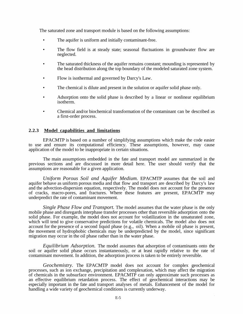
E-55
The saturated zone and transport module is based on the following assumptions:
• The aquifer is uniform and initially contaminant-free.
• The flow field is at steady state; seasonal fluctuations in groundwater flow areneglected.
• The saturated thickness of the aquifer remains constant; mounding is represented bythe head distribution along the top boundary of the modeled saturated zone system.
• Flow is isothermal and governed by Darcy's Law.
• The chemical is dilute and present in the solution or aquifer solid phase only.
• Adsorption onto the solid phase is described by a linear or nonlinear equilibriumisotherm.
• Chemical and/or biochemical transformation of the contaminant can be described asa first-order process.
2.2.3 Model capabilities and limitations
EPACMTP is based on a number of simplifying assumptions which make the code easierto use and ensure its computational efficiency. These assumptions, however, may causeapplication of the model to be inappropriate in certain situations.
The main assumptions embedded in the fate and transport model are summarized in theprevious sections and are discussed in more detail here. The user should verify that theassumptions are reasonable for a given application.
Uniform Porous Soil and Aquifer Medium. EPACMTP assumes that the soil andaquifer behave as uniform porous media and that flow and transport are described by Darcy's lawand the advection-dispersion equation, respectively. The model does not account for the presenceof cracks, macro-pores, and fractures. Where these features are present, EPACMTP mayunderpredict the rate of contaminant movement.
Single Phase Flow and Transport. The model assumes that the water phase is the onlymobile phase and disregards interphase transfer processes other than reversible adsorption onto thesolid phase. For example, the model does not account for volatilization in the unsaturated zone,which will tend to give conservative predictions for volatile chemicals. The model also does notaccount for the presence of a second liquid phase (e.g., oil). When a mobile oil phase is present,the movement of hydrophobic chemicals may be underpredicted by the model, since significantmigration may occur in the oil phase rather than in the water phase.
Equilibrium Adsorption. The model assumes that adsorption of contaminants onto thesoil or aquifer solid phase occurs instantaneously, or at least rapidly relative to the rate ofcontaminant movement. In addition, the adsorption process is taken to be entirely reversible.
Geochemistry. The EPACMTP model does not account for complex geochemicalprocesses, such as ion exchange, precipitation and complexation, which may affect the migrationof chemicals in the subsurface environment. EPACMTP can only approximate such processes asan effective equilibrium retardation process. The effect of geochemical interactions may beespecially important in the fate and transport analyses of metals. Enhancement of the model forhandling a wide variety of geochemical conditions is currently underway.
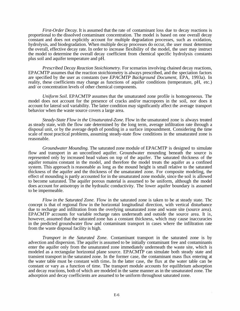
E-66
First-Order Decay. It is assumed that the rate of contaminant loss due to decay reactions isproportional to the dissolved contaminant concentration. The model is based on one overall decayconstant and does not explicitly account for multiple degradation processes, such as oxidation,hydrolysis, and biodegradation. When multiple decay processes do occur, the user must determinethe overall, effective decay rate. In order to increase flexibility of the model, the user may instructthe model to determine the overall decay coefficient from chemical specific hydrolysis constantsplus soil and aquifer temperature and pH.
Prescribed Decay Reaction Stoichiometry. For scenarios involving chained decay reactions,EPACMTP assumes that the reaction stoichiometry is always prescribed, and the speciation factorsare specified by the user as constants (see EPACMTP Background Document, EPA, 1993a). Inreality, these coefficients may change as functions of aquifer conditions (temperature, pH, etc.)and/ or concentration levels of other chemical components.
Uniform Soil. EPACMTP assumes that the unsaturated zone profile is homogeneous. Themodel does not account for the presence of cracks and/or macropores in the soil, nor does itaccount for lateral soil variability. The latter condition may significantly affect the average transportbehavior when the waste source covers a large area.
Steady-State Flow in the Unsaturated-Zone. Flow in the unsaturated zone is always treatedas steady state, with the flow rate determined by the long term, average infiltration rate through adisposal unit, or by the average depth of ponding in a surface impoundment. Considering the timescale of most practical problems, assuming steady-state flow conditions in the unsaturated zone isreasonable.
Groundwater Mounding. The saturated zone module of EPACMTP is designed to simulateflow and transport in an unconfined aquifer. Groundwater mounding beneath the source isrepresented only by increased head values on top of the aquifer. The saturated thickness of theaquifer remains constant in the model, and therefore the model treats the aquifer as a confinedsystem. This approach is reasonable as long as the mound height is small relative to the saturatedthickness of the aquifer and the thickness of the unsaturated zone. For composite modeling, theeffect of mounding is partly accounted for in the unsaturated zone module, since the soil is allowedto become saturated. The aquifer porous material is assumed to be uniform, although the modeldoes account for anisotropy in the hydraulic conductivity. The lower aquifer boundary is assumedto be impermeable.
Flow in the Saturated Zone. Flow in the saturated zone is taken to be at steady state. Thcconcept is that of regional flow in the horizontal longitudinal direction, with vertical disturbancedue to recharge and infiltration from the overlying unsaturated zone and waste site (source area).EPACMTP accounts for variable recharge rates underneath and outside the source area. It is,however, assumed that the saturated zone has a constant thickness, which may cause inaccuraciesin the predicted groundwater flow and contaminant transport in cases where the infiltration ratefrom the waste disposal facility is high.
Transport in the Saturated Zone. Contaminant transport in the saturated zone is byadvection and dispersion. The aquifer is assumed to be initially contaminant free and contaminantsenter the aquifer only from the unsaturated zone immediately underneath the waste site, which ismodeled as a rectangular horizontal plane source. EPACMTP can simulate both steady state andtransient transport in the saturated zone. In the former case, the contaminant mass flux entering atthe water table must be constant with time. In the latter case, the flux at the water table can beconstant or vary as a function of time. The transport module accounts for equilibrium adsorptionand decay reactions, both of which are modeled in the same manner as in the unsaturated zone. Theadsorption and decay coefficients are assumed to be uniform throughout saturated zone.

E-77
2.3 Monte Carlo Module
EPACMTP was designed to perform simulations on a nationwide basis, and to account forvariations of model input parameters reflecting variations in site and hydrogeological conditions.The fate and transport model is therefore linked to a Monte Carlo driver which generates modelinput parameter values from the probability distribution of each parameter. The Monte Carlomodeling procedure is described in more detail in this section.
The Monte Carlo method requires that for each input parameter, except constantparameters, a probability distribution is provided. The method involves the repeated generation ofpseudo-random values of the uncertain input variable(s) (drawn from the known distribution andwithin the range of any imposed bounds) and the application of the model using these values togenerate a series of model responses (receptor well concentration). These responses are thenstatistically analyzed to yield the cumulative probability distribution of the model output. Thus, thevarious steps involved in the application of the Monte Carlo simulation technique are:
(1) Selection of representative cumulative probability distribution functions for therelevant input variables.
(2) Generation of a pseudo-random number from the distributions selected in (1).These values represent a possible set of values (a realization) for the input variables.
(3) Application of the fate and transport simulation modules to compute the output(s),i.e., downstream well concentration.
(4) Repeated application of steps (2) and (3) for a specified number of iterations.
(5) Presentation of the series of output (random) values generated in step (3).
(6) Analysis of the Monte Carlo output to derive regulatory DAF values.
The Monte Carlo module designed for implementation with the EPACMTP compositemodel performs steps 2-5 above. This process is shown conceptually in Figure 2. Step 6 isperformed as a post-processing step. This last step simply involves converting the normalizedreceptor well concentrations to DAF values, and ranking then for high to low values. Each MonteCarlo iteration yields one DAF value for the constituent of concern (plus one DAF value for each ofthe transformation products, if the constituent is a degrader). Since each Monte Carlo iteration hasequal probability, ordering the DAF values from high to low, directly yields their cumulativeprobability distribution (CDF). If appropriate, CDF curves representing different regionaldistributions may be combined into a single CDF curve, which is a weighted average of theregional curves.
A simplified flow chart that illustrated the linking of the Monte Carlo module to thesimulation modules of the EPACMTP composite model is presented in Figure 3. The modelinginput data is read first, and subsequently the desired random numbers are generated. The generatedrandom and/ or derived parameter values are then assigned to the model variables. Following this,the contaminant transport fate and transport simulation is performed. The result is given in terms ofthe predicted contaminant concentration(s) in a down-stream receptor well. The generation ofrandom parameter values and fate and transport simulation is repeated as many times as desired todetermine the probability distribution of down-stream well concentrations.

E-88
Figure 2Conceptual Monte Carlo Framework For Deriving Probability Distribution
Of Model Output From Probability Distributions Of Input Parameters

E-99
Figure 3Flow Chart Of EPACMTP For Monte Carlo Simulation

E-101 0
2.3.1 Capabilities and Limitations of Monte Carlo Module
The Monte Carlo module in EPACMTP is implemented as a flexible module that canaccommodate a wide variety of input distributions. These include: constant, normal, lognormal,exponential, uniform, logl0 uniform, Johnson SB, empirical, or derived. In addition, specificupper and/or lower bounds can be provided for each parameter. The empirical distribution is usedwhen the data does not fit any of the other probability distributions. When the empiricaldistribution is used, the probability distribution is specified in tabular form as a list of parametervalues versus cumulative probability, from zero to one.
It is important to realize that the Monte Carlo method accounts for parameter variability anduncertainty; it does, however, not provide a way to account or compensate for process uncertainty.If the actual flow and transport processes that may occur at different sites, are different from thosesimulated in the fate and transport module, the result of a Monte Carlo analysis may not accuratelyreflect the actual variation in groundwater concentrations.
EPACMTP does not directly account for potential statistical dependencies, i.e., correlationsbetween parameters. The probability distributions of individual parameters are considered to bestatistically independent. At the same time, EPACMTP does incorporate a number of safeguardsagainst generating impossible combinations of model parameters. Lower and upper bounds on theparameters prevent unrealistically low or high values from being generated at all.
In the case of model parameters that have a direct physical dependence on other parameters,these parameters can be specified as derived parameters. For instance, the ambient groundwaterflow rate is determined by the regional hydraulic gradient and the aquifer hydraulic conductivity. Inthe Monte Carlo analyses, the ambient groundwater flow rate is therefore calculated as the productof conductivity and gradient, rather than generated independently. A detailed discussion of thederived parameters used in the model is provided in the EPACMTP User's Guide (EPA, 1994).

E-111 1
3.0 MODELING PROCEDURE
This section documents the modeling procedure followed in determining the groundwaterpathway DAF values for the Soil Screening Levels. Section 3.1 describes the overall approach forthe modeling analysis; section 3.2 describes the model options used and summarizes the inputparameter values.
3.1 Modeling Approach
The overall modeling approach consisted of two stages. First, a sensitivity analysis wasperformed to determine the optimal number of Monte Carlo repetitions required to achieve a stableand converged result, and to determine which site-related parameters have the greatest impact onthe DAFs. Secondly, Monte Carlo analyses were performed to determined DAF values as afunction of the size of the source area, for various scenarios of receptor well placement.
3.1.1 Determination of Monte Carlo Repetition Number and Sensitivity Analysis
The criterion for determining the optimal number of Monte Carlo repetitions was set to achange in DAF value of no more than 5 percent when the number of repetitions is varied. A MonteCarlo simulation comprising 20,000 repetitions was first made. The results from this simulationwere analyzed by calculating the 85th percentile DAP value obtained by sampling model outputsequences of different length, from 2,000 to the full 20,000 repetitions. The modeling scenarioconsidered in this analysis was the same as that in the base case scenario discussed in the nextsection, with the size of the source area set to 10,000 m2.
The sensitivity analysis on site-related model parameters was performed by fixing oneparameter at a time, while remaining model parameters were varied according to their default,nationwide probability distributions as discussed in the EPACMTP User's Guide (EPA, 1993b).
For each parameter, the low, medium, and high values were selected, corresponding to the15th, 50th, and 85th percentile, respectively, of that parameter's probability distribution. As aresult, the sensitivity analysis reflects, in part, the width of each parameter's probabilitydistribution. Parameters with a narrow range of variation will tend to be among the less sensitiveparameters, and vice versa for parameters that have a wide range of variation. By conducting thesensitivity analysis as a series of Monte Carlo simulations, any parameter interactions on the modeloutput are automatically accounted for. Each of the Monte Carlo simulations yields a probabilitydistribution of predicted receptor well concentrations. Evaluating the distributions obtained withdifferent fixed values of the same parameter provides a measure of the overall sensitivity andimpact of that parameter. In each case the model was run for 2,000 Monte Carlo iterations.Steady-state conditions (continuous source) were simulated in all cases.
In a complete Monte Carlo analysis, over 20 different model parameters are involved.These parameters may be divided into two broad categories. The first includes parameters that areindependent of contaminant-specific chemical properties, e.g., depth to water table, aquiferthickness, receptor well distance, etc. The second category encompasses those parameters that arerelated to contaminant-specific sorption and biochemical transformation characteristics. Thiscategory includes the organic carbon partition coefficient, but also parameters such as aquifer pH,temperature and fraction organic carbon. The sensitivity of the model to the first category ofparameters has examined, by considering a non-degrading, non-sorbing contaminant. Under theseconditions, any parameters in the second category will have zero sensitivity. In addition, allunsaturated zone parameters can be left out of the analysis, since the predicted steady statecontaminant concentration at the water table will always be the same as that entering the unsaturated

E-121 2
zone. The only exception to this is the soil type parameter. In the nationwide Monte Carlomodeling approach, different soil types are distinguished. Each of the three different soil types(sandy loam, silt loam or silty clay loam) has a different distribution of infiltration rate, with thesandy loam soil type having the highest infiltration rates, silty clay loam having the lowest, andsilty loam having intermediate rates. The effect of the soil type parameter is thus intermixed withthat of infiltration rate. Table 1 lists the input 'low', 'medium' and 'high' values for all theparameters examined.
Table 1Parameter input values for model sensitivity analysis.
Parameter Low Median High
Source Parameters
Source Area (m2) 4.8x10⁴ 2.8x 10⁵ 1.1 x10⁶
Infiltration Rate (m/yr) 6.0x10⁻⁴ 6.4x10⁻³ 1.7x10⁻¹
Recharge Rate (m/yr) 6.0x10⁻⁴ 8.0x10⁻³ 1.5x10⁻¹
Saturated Zone Parameters
Saturated Thickness (m) 15.55 60.8 159.3
Hydraulic conductivity (m/yr) 1.9 x 10³ 1.5 x 10⁴ 5.5 X 10⁴
Regional gradient 4.3 x 10⁻³ 1.8 x 10⁻² 5.0 X 10⁻²
Ambient groundwater velocity (m/yr) 53.2 404.0 2883.0
Porosity 0.374 0.415 0.455
Longitudinal Dispersivity (m) 4.2 12.7 98.5
Transverse Dispersivity (m) 0.53 1.59 12.31
Vertical Dispersivity (m) 0.026 0.079 0.62.
3.1.2 Analysis of DAF Values for Different Source Areas
Following completion of the sensitivity analysis discussed above, an analysis wasperformed of the variation of DAF values with size of the contaminated area. The sensitivityanalysis, results of which are presented in Section 4.1, showed that the size of the contaminatedsource area is one of the most sensitive parameters in the model. For the purpose of deriving DAFvalues for the groundwater pathway in determining soil screening levels, it would therefore beappropriate to correlate the DAF value to the size of the contaminated area.
The EPACMTP modeling analysis was designed to determine the size of the contaminatedarea that would result in DAF values of 10 and 100 at the upper 85th, 90th, and 95th percentile ofprobability, respectively. Since it is not possible to directly determine the source area that results ina specific DAF value, the model was executed for a range of different source areas, using adifferent but fixed source area value in each Monte Carlo simulation. The 85th, 90th, and 95thpercentile DAF values were then plotted against source area, in order to determine the value ofsource area corresponding to a specific DAF value.

E-131 3
3.1.2.1 Model Options and Input Parameters
Table 2 summarizes the EPACMTP model options used in performing the simulations. Modelinput parameters used are summarized in Table 3. The selected options and input parameterdistributions and values are consistent with those used in the default nationwide modeling, and arediscussed individually in the EPACMTP User's Guide (EPA, 1994). Exceptions to this defaultmodeling scenario are discussed below.
Table 2Summary of EPACMTP modeling options.
Option Value Selected
Simulation Type Monte Carlo
Number of Repetitions 15,000
Nationwide Aggregation Yes
Source Type Continuous
Unsat. Zone Present Yes
Sat. Zone Model Quasi-3D
Contaminant Degradation No
Contaminant Sorption No
Source Area
In the default, nationwide modeling scenario, the waste site area, or source area, is treatedas a Monte Carlo variable, with a distribution of values equal to that of the type of waste unit, e.g.landfills, considered. In the present modeling analyses, the source area was set to a different butconstant value in each simulation run.
Receptor Well Location
In the default nationwide modeling scenario, the position of the nearest downgradientreceptor well in the saturated zone is treated as a Monte Carlo variable. The position of the well isdefined by its x-, y-, and z-coordinates. The x-coordinate represents the distance along the ambientgroundwater flow direction from the downgradient edge of the contaminated area. They-coordinate represents the horizontal transverse distance of the well from the plume centerline.The x-, and y-coordinate in turn can be defined in terms of an overall downgradient distance, andan angle off-center (EPA, 1994). The z-coordinate represents the depth of the well intake pointbelow the water table. This is illustrated schematically in Figure 4, which shows the receptor welllocation in both plan view and cross-sectional view.
In the default nationwide modeling scenario, the x-, and z-coordinates of the well aredetermined from Agency surveys on the distance of residential wells from municipal landfills, anddata on the depth of residential drinking water wells, respectively. The y-coordinate value isdetermined so that the well location falls within the approximate areal extent of the contaminantplume (see Figure 4).
For the present modeling analysis, a number of different receptor well placement scenarioswere considered. These scenarios are summarized in Table 4.

E-141 4
Table 3Summary of EPACMTP input parameters.
Parameter Value or Distribution Type Comment
Source-Specific
Area Constant Varied in each run
Infiltration Rate Soil-type dependent default
Recharge Rate Soil-type dependent default
Leachate Concentration = 1.0 default
Chemical-Specific
Hydrolysis Rate Constants = 0.0 Contaminant does not degrade
Organic Carbon Partition Coeff. = 0.0 Contaminant does not sorb
Unsaturated Zone Specific
Depth to Water Table Empirical default
Dispersivity Soil-depth dependent default
Soil Hydraulic Properties Soil-type dependent default
Soil Chemical Properties Soil-type dependent default
Saturated Zone Specific
Sat. Zone Thickness Exponential default
Hydraulic Conductivity Derived from Part. Diam. default
Hydraulic Gradient Exponential default
Seepage Velocity Derived from Conductivity andGradient
default
Particle Diameter Empirical default
Porosity Derived from Part. Diam default
Bulk Density Derived from Porosity default
Longitudinal Dispersivity Distance-dependent default
Transverse Dispersivity Derived from Long. Dispersivity default
Vertical Dispersivity Derived from Long. Dispersivity default
Receptor Well x-coordinate = 25 feet Set to fixed value
Receptor Well y-coordinate Within plume default
Receptor Well z-coordinate Empirical default
Note: 'Default' represents default nationwide Monte Carlo scenario as presented in EPACMTP User'sGuide (EPA, 1994).

E-151 5
Figure 4Plain View And Cross-Section View Showing Location Of Receptor Well

E-161 6
Table 4Receptor Well Location Scenarios
Scenario Xwell Ywell Zwell
1 (Base Case) 25 ft from edge of sourcearea
Monte Carlo within plume Nationwide Distribution
2 Nationwide Distribution Monte Carlo within plume Nationwide Distribution
3 0 ft from edge of sourcearea
Monte Carlo within half-width of source area
Nationwide Distribution
4 25 ft from edge of sourcearea
Monte Carlo within half-width of source area
Nationwide Distribution
5 100 ft from edge ofsource area
Monte Carlo within half-width of source area
Nationwide Distribution
6 25 ft from edge of sourcearea
Width of source area + 25ft
25 ft below water table
Xwell = Downgradient distance of receptor well from edge of source area.Ywell = Horizontal transverse distance from plume centerline.Zwell = Depth of well intake point below water tablet
The base case scenario (scenario 1) involved setting the x-distance of the receptor well to25 feet from the edge of the source area. Nationwide default options were used for the receptorwell y- and z-coordinates. The y-coordinate of the well was assigned a uniform probabilitydistribution within the boundary of the plume. The depth of the well intake point (z-coordinate)was assumed to vary within upper and lower bounds of 15 and 300 feet below the water table,reflecting a national sample distribution of depths of residential drinking water wells (EPA, 1994).
In addition to this base case scenario, a number of other well placement scenarios wereinvestigated also. These are numbered in Table 4 as scenarios 2 through 6. Scenario 2 correspondsto the default, nationwide Monte Carlo modeling scenario in which the x, y, and z locations of thewell are all variable. In scenarios 3, 4 and 5, the distance between the receptor well and the sourcearea is varied from zero to 100 feet. In these scenarios, the ycoordinate of the well was constrainedto the central portion of the plume. In scenario number 6, the x-, y-, and z-coordinates of thereceptor well were all set to constant values. These additional scenarios were included in theanalysis in order to assess the sensitivity of the model results to the location of the receptor well.
Aquifer Particle Size Distribution
In the default Monte Carlo modeling scenario, the aquifer hydraulic conductivity, porosity,and bulk density are determined from the mean particle diameter. The particle diameter distributionused is based on data compiled by Shea (1974). In the present modeling analyses for fixed wastesite areas, the same approach and data were used, but the distribution was shifted somewhat toassign more weight to the smallest particle diameter interval. The result is that lower values of thehydraulic conductivity values generated, and also of the ambient groundwater seepage velocities,received more emphasis. Lower ambient groundwater velocities reduce the degree of dilution of theincoming contaminant plume and therefore result in lower, i.e. more conservative, DAF values.Table 5 summarizes the distribution of particle size diameters used in both the default nationwidemodeling scenario and in the present analyses.

E-171 7
Table 5Distribution of aquifer particle diameter.
Nationwide Default Present Analyses
Particle Diameter (cm)
CumulativeProbability
Particle Diameter(cm)
CumulativeProbability
3.9 10-4 0.000 4.0 10-4 0.100
7.8 10-4 0.038 8.0 10-4 0.150
1.6 10-3 0.104 1.6 10-3 0.200
3.1 10-3 0.171 3.1 10-3 0.270
6.3 10-3 0.262 6.3 10-3 0.330
1.25 10-2 0.371 1.25 10-2 0.440
2.5 10-2 0.560 2.5 10-2 0.590
5.0 10-2 0.792 5.0 10-2 0.790
1.0 10-1 0.904 1.0 10-1 0.880
2.0 10-1 0.944 2.0 10-1 0.910
4.0 10-1 0.946 4.0 10-1 0.940
8.0 10-1 1.000 7.5 10-1 1.000

E-181 8
4.0 RESULTS
This section presents the results of the modeling analyses performed. The analysis of theconvergence of the Monte Carlo simulation is presented first, followed by the parameter sensitivityanalysis, and thirdly the analysis of DAF values as a function of source area for various wellplacement scenarios.
4.1 Convergence of Monte Carlo Simulation
Table 6 summarizes the results of this convergence analysis. It shows the variation of the85th percentile DAF value with the number of Monte Carlo repetitions, from 2,000 to 20,000. Thevariations in DAF values are shown both as absolute and relative differences. The table shows thatfor this example, the DAF generally increases with the number of Monte Carlo repetitions. Itshould be kept in mind that the results from different repetition numbers as presented in the table,are not independent of one another. For instance, the first 2,000 repetitions are also incorporated inthe 5000 repetition results, which in turn is in the 10,000 repetition result, etc. The rightmostcolumn of Table 6 shows the percentage difference in DAF value between different repetitionnumbers. At repetition numbers of 14,000 or less, the percentage difference varies in a somewhatirregular manner. However, for repetition numbers of 15,000 or greater, the DAF remainedrelatively constant, with incremental changes of DAF remaining at 1 % or less. Based upon theseresults, a repetition number of 15,000 was selected for use in the subsequent runs with fixedsource area.
4.2 Parameter Sensitivity Analysis
Results of the parameter sensitivity analysis are summarized in Table 7. The parameters areranked in this table in order of relative sensitivity. Relative sensitivity is defined for this purpose asthe absolute difference between the "high" and "low" DAF at the 85th percentile level, divided bythe 85th percentile DAF for the "median" case.
The table shows that the most sensitive parameters included the rate of infiltration, which isa function of soil type, the saturated thickness of the aquifer, the size of source area, thegroundwater seepage velocity, and the vertical position of the receptor well below the water table.The least sensitive parameters included porosity, downstream distance of the receptor well in boththe x- and y-directions, the horizontal transverse dispersivity, and the areal recharge rate. Tointerpret these results, it should be kept in mind that the rankings reflect in part the range ofvariation of each parameter in the data set used for the sensitivity analysis. The infiltration rate wasa highly sensitive parameter since, for a given leachate concentration, it directly affects the massflux of contaminant entering the subsurface. The size of the source would be expected to be equallysensitive, were it not for the fact that in the sensitivity analysis, the source area had a muchnarrower range of variation than the infiltration rate. The "high" and "low" values of the sourcearea, which were taken from a nationwide distribution of landfill waste units, varied by a factor of23, while the ratio of "high" to "low" infiltration rate was almost 300.
In the simulations performed for the sensitivity analysis, no constraint was imposed on thevertical position of the well. The well was modeled as having a uniform distribution with the wellintake point located anywhere between the water table and the base of the aquifer. The aquifersaturated thickness and vertical position of the well were both among the sensitive parameters, withsimilar effects on DAF values. Increasing either the saturated thickness, or the fractional depth ofthe receptor well below the water table, increases the likelihood that the receptor well will belocated underneath the contaminant plume and sample uncontaminated groundwater, leading to a
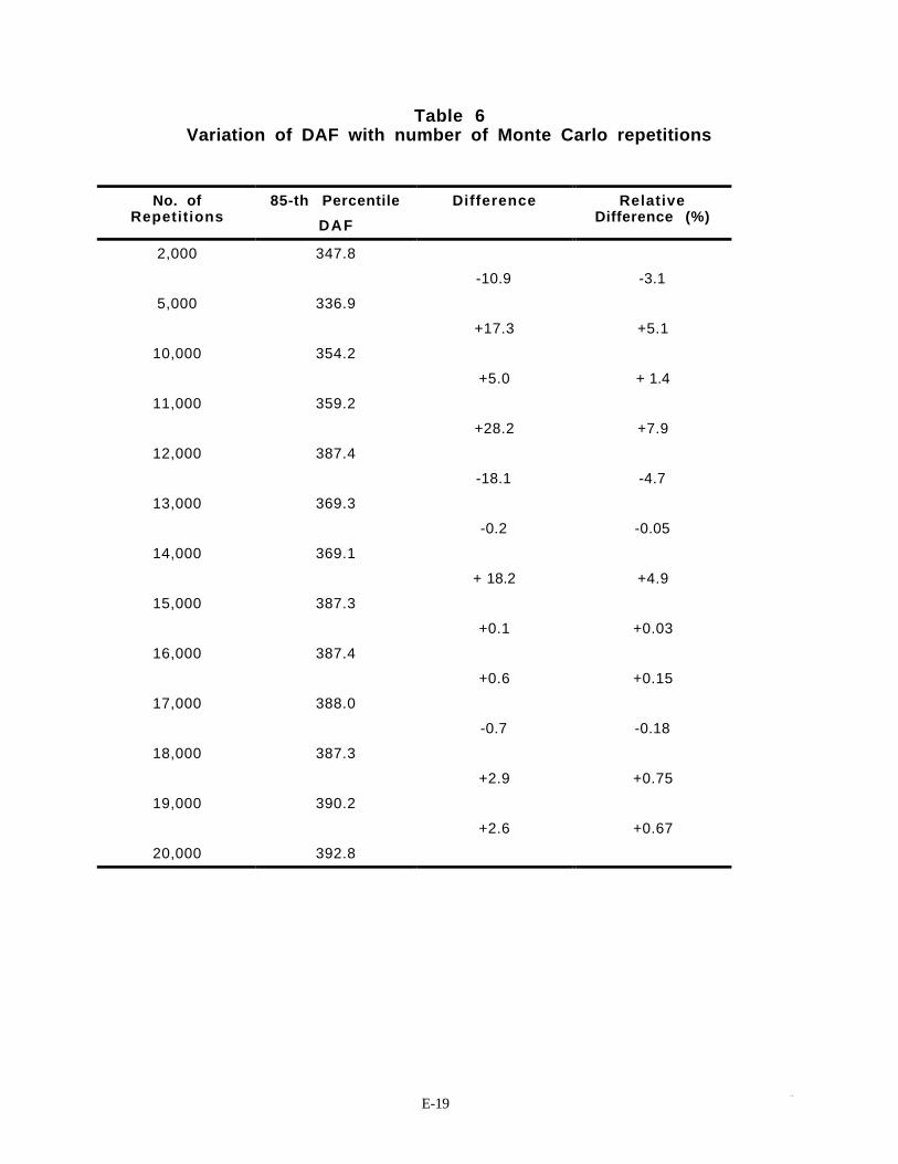
E-191 9
Table 6Variation of DAF with number of Monte Carlo repetitions
No. ofRepetitions
85-th Percentile
DAF
Difference RelativeDifference (%)
2,000 347.8
-10.9 -3.1
5,000 336.9
+17.3 +5.1
10,000 354.2
+5.0 + 1.4
11,000 359.2
+28.2 +7.9
12,000 387.4
-18.1 -4.7
13,000 369.3
-0.2 -0.05
14,000 369.1
+ 18.2 +4.9
15,000 387.3
+0.1 +0.03
16,000 387.4
+0.6 +0.15
17,000 388.0
-0.7 -0.18
18,000 387.3
+2.9 +0.75
19,000 390.2
+2.6 +0.67
20,000 392.8
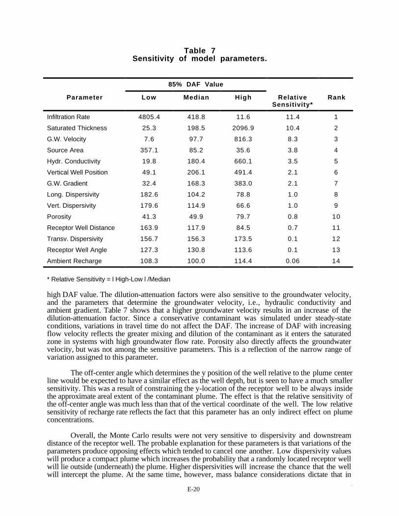
E-202 0
Table 7Sensitivity of model parameters.
85% DAF Value
Parameter Low Median High RelativeSensitivity*
Rank
Infiltration Rate 4805.4 418.8 11.6 11.4 1
Saturated Thickness 25.3 198.5 2096.9 10.4 2
G.W. Velocity 7.6 97.7 816.3 8.3 3
Source Area 357.1 85.2 35.6 3.8 4
Hydr. Conductivity 19.8 180.4 660.1 3.5 5
Vertical Well Position 49.1 206.1 491.4 2.1 6
G.W. Gradient 32.4 168.3 383.0 2.1 7
Long. Dispersivity 182.6 104.2 78.8 1.0 8
Vert. Dispersivity 179.6 114.9 66.6 1.0 9
Porosity 41.3 49.9 79.7 0.8 10
Receptor Well Distance 163.9 117.9 84.5 0.7 11
Transv. Dispersivity 156.7 156.3 173.5 0.1 12
Receptor Well Angle 127.3 130.8 113.6 0.1 13
Ambient Recharge 108.3 100.0 114.4 0.06 14_
* Relative Sensitivity = l High-Low l /Median
high DAF value. The dilution-attenuation factors were also sensitive to the groundwater velocity,and the parameters that determine the groundwater velocity, i.e., hydraulic conductivity andambient gradient. Table 7 shows that a higher groundwater velocity results in an increase of thedilution-attenuation factor. Since a conservative contaminant was simulated under steady-stateconditions, variations in travel time do not affect the DAF. The increase of DAF with increasingflow velocity reflects the greater mixing and dilution of the contaminant as it enters the saturatedzone in systems with high groundwater flow rate. Porosity also directly affects the groundwatervelocity, but was not among the sensitive parameters. This is a reflection of the narrow range ofvariation assigned to this parameter.
The off-center angle which determines the y position of the well relative to the plume centerline would be expected to have a similar effect as the well depth, but is seen to have a much smallersensitivity. This was a result of constraining the y-location of the receptor well to be always insidethe approximate areal extent of the contaminant plume. The effect is that the relative sensitivity ofthe off-center angle was much less than that of the vertical coordinate of the well. The low relativesensitivity of recharge rate reflects the fact that this parameter has an only indirect effect on plumeconcentrations.
Overall, the Monte Carlo results were not very sensitive to dispersivity and downstreamdistance of the receptor well. The probable explanation for these parameters is that variations of theparameters produce opposing effects which tended to cancel one another. Low dispersivity valueswill produce a compact plume which increases the probability that a randomly located receptor wellwill lie outside (underneath) the plume. Higher dispersivities will increase the chance that the wellwill intercept the plume. At the same time, however, mass balance considerations dictate that in
E-212 1
this case average concentrations inside the plume will be lower than in the low dispersivity case.Similar reasoning applies to the effect of receptor well distance. If the well is located near thesource, concentrations in the plume will be relatively high, but so is the chance that the well doesnot intercept the plume at all. At greater distances from the source, the likelihood that the well islocated inside the plume is greater, but the plume will also be more diluted. In the course of a fullMonte Carlo simulation these opposing effects would tend to average out. The much lowersensitivity of transverse dispersivity, αT, compared to αL and αV can be contributed to the imposedconstraint that the well must always be within the areal extent of the plume.
The results of the sensitivity analysis show that the site characteristic which lends itselfbest for a classification system for correlating sites to DAF values is the size of the contaminated(or source) area. In the subsequent analyses, the DAF values were therefore determined as afunction of the source area size. These results are presented in the following section.
4.3 DAF Values as a Function of Source Area
This section presents the DAF value as a function of source area for various well locationscenarios. The results for each of the scenarios examined are presented in tabular and graphicalform. Figure 5 shows the variation of the 85th, 90th, and 95th percentile DAF with source area forthe base case scenario. The source area is expressed in square feet. The figure displays DAFagainst source area in a log-log graph. The graph shows an approximately linear relationshipexcept that at very large values of the source area, the DAF starts to level off. Eventually the DAFapproaches a value of 1.0. As expected, the curve for the 95th percentile DAF always shows thelowest DAF values, while the 85th percentile shows the highest DAFs. The DAF versus sourcearea relationship for the other well placement scenarios are shown in Figures 6 through 10. Thenumerical results for each scenario are summarized in Tables Al through A6 in the appendix.
Inspection and comparison of the results for each scenario indicate that the relationshipfollows the same general shape in each case, but the magnitude of DAF values at a given sourcearea can be quite different for different well placement scenarios. In order to allow a directcomparison between the various scenarios analyzed, the DAF values obtained for a source area of150,000 ft2 (3.4 acres) are shown in Table 8 as a function of the receptor well location scenario.
Inspection of the DAF values shows that the default nationwide scenario for locating thereceptor well results in the highest DAF values, as compared to the base case scenario and the otherscenarios, in which the receptor well location was fixed at a relatively close distance from the wastesource. In the default nationwide modeling scenario, the well location is assigned from nationwidedata on both the distance from the waste source and depth of the well intake point below the watertable. In the default nationwide modeling scenario, the receptor well is allowed to be located up to1 mile from the waste source. In the base case (Scenario 1) the well is allowed to be locatedanywhere within the areal extent of the contaminant plume for a fixed x-distance of 25 feet. Thisallows the well to be located near the fringes of the contaminant plume where concentrations arerelatively low and DAF values are correspondingly high. In contrast, in Scenarios 3, 4, and 5, thewell location was constrained to be within the half-width of the waste source. In other words, thewell was always placed in the central portion of the contaminant plume where concentrations arehighest. As a result, these scenarios show lower DAF values then the base case scenario. Theresults for Scenarios 3, 4, and 5, which differ only in the x-distance of the receptor well, show thatplacement of the well at either 25 or 100 feet away from the waste source results in 85% and 90%DAF values that are actually lower, i.e. more conservative, than placement of the well directly atthe edge of the waste source. This is a counter-intuitive result, but may be explained from theinteraction between distance from the waste source and vertical extent of the contaminant plumebelow the water table. Close to the waste source, the contaminant concentrations within the plumeare highest, but the plume may not have penetrated very deeply into the saturated zone (Figure 2).
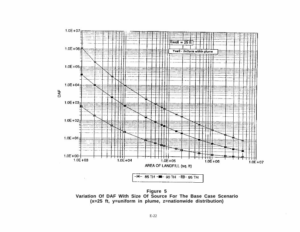
E-222 2
Figure 5Variation Of DAF With Size Of Source For The Base Case Scenario
(x=25 ft, y=uniform in plume, z=nationwide distribution)

E-232 3
Figure 6Variation Of DAF With Size Of Source Area For The Default Nationwided Scenario
(Scenario 2: x=nationwide distribution, y=uniform in plume, z=nationwide distribution)

E-242 4
Figure 7Variation Of DAF With Size Of Source Area For Scenario 3
(x=0, y=uniform within half-width of source area, z=nationwide distribution

E-252 5
Figure 8Variation Of DAF With Size Of Source Area For Scenario 4
(x=25 fy, y=uniform within half-width of source area, z=nationwide distribution)

E-262 6
Figure 9Variation Of DAF With Size Of Source Area For Scenario 5
(x=100 ft, y=uniform within half-width of source area, z=nationwide distribution)

E-272 7
Figure 10Variation Of DAF With Size Of Source Area For Scenario 6
(x=25 ft, y=width of source area + 25 ft, z=25 ft)

E-282 8
Table 8DAF values for waste site area of 150,000 ft2.
DAF Percentile
Model Scenario 8 5 9 0 9 5
1 (base case) 237.5 26.4 2.8
2 300.1 114.7 26.8
3 158.8 17.9 1.7
4 132.1 16.6 1.8
5 98.8 15.1 2.0
6 94.7 25.3 4.4
Because the vertical position of the well was taken as a random variable, with a maximum value ofup to 300 feet, the probability that a receptor well samples pristine groundwater underneath thecontaminant plume is higher at close distances from the waste area. Conversely, as the distancefrom the source increases, the plume becomes more dilute but also extends deeper below the watertable. The final result is that the overall DAF may actually decrease with distance from the source.The table also shows that at the 95% level, the lowest DAF is obtained in the case where the well islocated at the edge of the waste source. This reflects that the highest concentration values will beobtained only very close to the waste source.
The results for the last scenario, in which the x, y, and z locations of the receptor well wereall fixed, show that fixing the well depth at 25 feet ensures that the well is placed shallow enoughthat it will be located inside the plume in nearly all cases, resulting in low DAF values at the 85thand 90th percentile values. On the other hand, the well in this case is never placed immediately atthe plume centerline, so that the highest concentrations sampled in this scenario are always lowerthan in the other scenarios. This is reflected in the higher DAF value at the 95th percentile level.
One of the key objectives of the present analyses was to determine the appropriategroundwater DAF value for a waste area of given size. For the base case scenario, the 90thpercentile DAF value is on the order of 100 or higher for a waste area size of 1 acre (43,560 ft2)and less. For waste areas of 10 acres and greater, the 90th percentile DAF is 10 or less.

E-292 9
REFERENCES
Shea, J.H., 1974. Deficiencies of elastic particles of certain sizes. Journal of SedimentaryPetrology, 44:905-1003.
U.S. EPA, 1993a. EPA's Composite Model for Leachate Migration with Transformation Products:EPACMTP. Volume I: Background Document. Office of Solid Waste, July 1993.
U.S. EPA, 1993b. Draft Soil Screening Level Guidance Quick Reference Fact Sheet. Office ofSolid Waste and Emergency Response, September 1993.
U.S. EPA, 1994. Modeling Approach for Simulating Three-Dimensional Migration of Land andDisposal Leachate with Transformation Products and Consideration of Water-TableMounding. Volume II: User's Guide for EPA's Composite Model for Leachate Migrationwith Transformation Products (EPACMTP). Office of Solid Waste, May 1994.

E-303 0
APPENDIX A

E-313 1
Table A1 DAF values as a function of source area for base casescenario (x=25 ft., y=uniform in plume, z-nationwidedistribution).
DAF
Area (sq. ft.) 8 5 t h 9 0 t h 9 5 t h
1000 1.09E+06 3.76E+04 609.01
2000 1.86E+05 9.63E+03 187.69
5000 2.91 E+04 2.00E+03 53.02
10000 9.31 E+03 680.27 22.57
30000 1647.18 155.21 7.82
50000 869.57 84.25 5.41
70000 569.80 59.28 4.34
80000 477.33 50.56 3.97
150000 237.47 26.36 2.77
200000 174.86 20.19 2.37
500000 64.52 9.12 1.61
1000000 32.27 5.61 1.32
2000000 17.83 3.68 1.16
3000000 12.94 2.94 1.11
5000000 8.91 2.33 1.06

E-323 2
Table A2 DAF values as a function of source area for Scenario 2(x=nationwide distribution, y=uniform in plume, z=nationwidedistribution).
DAFArea (sq. ft.) 8 5 t h 9 0 t h 9 5 t h
5000 6222.78 2425.42 565.618000 3977.72 1573.32 371.06
10000 3215.43 1286.01 298.7845000 817.66 315.06 73.4850000 745.16 288.27 67.20
100000 424.81 160.82 38.11150000 300.12 114.71 26.82220000 218.87 82.30 20.00500000 110.35 40.10 10.92
1000000 63.45 23.75 6.225000000 21.03 7.85 2.556000000 19.06 7.01 2.39

E-333 3
Table A3 DAF values as a function of source area for Scenario 3 (x=0ft, y=uniform within half-width of source area, z=nationwidedistribution).
DAFArea (sq. ft.) 8 5 t h 9 0 t h 9 5 t h
1000 1.42E+07 2.09E+05 946.07
2000 9.19E+05 2.83E+04 211.15
5000 5.54E+04 2.74E+ 03 44.23
10000 1.16E+04 644.33 15.29
30000 1.43E+03 120.42 4.48
50000 668.45 60.02 3.10
70000 417.19 37.97 2.53
80000 350.39 33.16 2.34
150000 158.76 17.87 1.74
200000 114.63 12.96 1.56
500000 40.55 5.54 1.23
1000000 21.13 3.50 1.15
2000000 11.58 2.38 1.08
3000000 8.66 1.98 1.06

E-343 4
Table A4 DAF values as a function of source area for Scenario 4 (x=25ft, y=uniform within half-width of source area, z=nationwidedistribution).
DAF
Area (sq. ft.) 8 5 t h 9 0 t h 9 5 t h
1000 5.93E + 05 2.07E + 04 348.31
2000 1.09E+05 4.92E+03 118.11
5000 1.64E + 04 1.03E + 03 29.86
10000 4.89E+03 352.49 13.14
30000 928.51 93.98 4.73
50000 490.20 49.78 3.28
70000 323.42 34.79 2.69
80000 272.85 29.82 2.47
150000 132.05 16.55 1.82
200000 97.94 12.29 1.61
500000 37.99 5.50 1.29
1000000 20.08 3.50 1.17
2000000 11.35 2.40 1.10
3000000 8.49 2.00 1.07

E-353 5
Table A5 DAF values as a function of source area for Scenario 5(x=100 ft, y=uniform within half-width of source, z=nationwidedistribution).
DAF
Area (sq. ft.) 8 5 t h 9 0 t h 9 5 t h
1000 4.24E+04 3.43E+03 181.88
2000 1.52E + 04 1.33E + 03 74.79
5000 4.24E+ 03 437.25 27.23
10000 1.81 E+03 204.29 13.09
30000 497.27 68.21 5.10
50000 293.34 40.72 3.71
70000 207.77 29.89 2.96
80000 184.57 26.86 2.73
150000 98.81 15.05 2.03
200000 74.63 11.55 1.82
500000 32.99 5.83 1.40
1000000 18.66 3.71 1.26
2000000 11.14 2.53 1.16
3000000 8.33 2.09 1.13

E-363 6
Table A6 DAF values as a function of source area for Scenario 6 (x=25ft, y=source width + 25 ft, z=25 ft).
DAF
Area (sq. ft.) 8 5 t h 9 0 t h 9 5 t h
1200 44247.79 10479.98 1004.72
1500 30759.77 7215.01 744.05
5000 4789.27 1273.40 140.81
7500 2698.33 725.69 82.51
23000 637.76 155.16 21.82
26000 544.66 135.91 18.84
29000 482.63 121.43 16.52
100000 139.66 35.55 5.56
170000 76.69 21.24 3.94
250000 50.40 15.04 3.19
800000 18.10 6.04 1.81
1800000 10.26 3.87 1.48

APPENDIX F
Dilution Factor Modeling Results

F-1
Dilution Factor Model Results: DNAPL Sites
Source size (acres) 0.5 10 30 100 600Source length (m) 45 201 349 636 1,559Aquifer thickness (m) 9.1
Infiltration by Average GW Mixing zone depth Dilution factor
Hyd. Region Velocity (m/yr) Site size (acres) Site size (acres)Site Name State Region (m/yr) Seepage Darcy 0.5 10 30 100 600 0.5 10 30 100 600Army Creek Landfill DE 10 0.24 5,563 1,947 5 21 37 67 165 861 370 214 118 49Atlantic Wood Ind. VA 10 0.24 1,261 442 5 21 37 68 166 197 85 49 27 12AtlasTack Corp. MA 9 0.22 3 1 10 30 46 76 174 2 1 1 1 1Auburn Rd. Landfill NH 9 0.22 61 21 5 23 40 72 173 12 5 4 2 2Baird & McGuire MA 9 0.22 61 21 5 23 40 72 173 12 5 4 2 2Bally Groundwater PA 6 0.15 3,204 1,121 5 21 37 67 165 793 341 197 108 45Beacon Hts. Landfill CT 9 0.22 15 5 6 27 44 76 174 4 2 2 1 1Berks Sand Pit PA 6 0.15 10 4 6 27 44 76 174 4 2 2 1 1Brodhead Creek PA 7 0.20 11,246 3,936 5 21 37 67 165 2,085 895 517 284 116Brunswick Naval Air Sta. ME 9 0.22 230 81 5 22 38 69 168 41 18 11 6 3Cannon Eng.- Bridgewater MA 9 0.22 3 1 11 30 46 76 174 2 1 1 1 1Central Landfill RI 9 0.22 223 78 5 22 38 69 168 39 17 10 6 3Centre County Kepone PA 6 0.15 61,189 21,416 5 21 37 67 165 15,112 6,489 3,747 2,053 839Chas.-Geo. Reclam. Trust MA 9 0.22 34 12 6 24 42 74 174 8 3 2 2 1Coakley Landfill NH 9 0.22 113 40 5 22 39 70 171 21 9 6 4 2Craig Farm Drum PA 6 0.15 451 158 5 21 37 68 166 113 49 29 16 7Davis Liquid Waste Rl 9 0.22 189 66 5 22 38 69 169 34 15 9 5 3Delaware City PVC DE 10 0.24 223 78 5 22 38 69 169 36 16 10 6 3Dorney Road Landfill PA 6 0.15 1,913 670 5 21 37 67 165 474 204 118 65 27Dover Mun. Landfill NH 9 0.22 289 101 5 22 38 69 168 51 22 13 8 4DuPont-Newport DE 10 0.24 33 12 6 25 42 74 174 7 3 2 2 1Dublin TCE Site PA 6 0.15 32 11 5 24 41 73 173 10 4 3 2 1Durham Meadows CT 9 0.22 612 214 5 21 37 68 166 105 45 27 15 7East Mt. Zion PA 6 0.15 1,218 426 5 21 37 68 165 303 130 76 42 18Elizabethtown Landfill PA 6 0.15 56 20 5 23 39 71 172 16 7 4 3 2Gallup's Quarry CT 9 0.22 67 23 5 23 40 72 172 13 6 4 3 2Greenwood Chemical VA 8 0.15 3 1 10 30 46 76 174 2 1 1 1 1Groveland Wells MA 9 0.22 612 214 5 21 37 68 166 105 45 27 15 7Halby Chemical Co. DE 10 0.24 5 2 9 30 46 76 174 2 1 1 1 1Harvey & Knott Drum DE 10 0.24 434 152 5 22 37 68 167 69 30 18 10 5Havertown PCP PA 8 0.15 24 9 6 24 41 74 174 8 4 2 2 1Heleva Landfill PA 6 0.15 28 10 5 24 41 73 173 9 4 3 2 1Henderson Road PA 6 0.15 834 292 5 21 37 68 166 208 89 52 29 12Hocomonco Pond MA 9 0.22 1,986 695 5 21 37 68 165 336 145 84 46 20Holton Circle NH 9 0.22 2,809 983 5 21 37 67 165 475 204 118 65 27Hunterstown Road PA 6 0.15 562 197 5 21 37 68 166 141 61 35 20 9Industri-plex MA 9 0.22 289 101 5 22 38 69 168 51 22 13 8 4Kane and Lombard Street MD 8 0.15 681 238 5 21 37 68 166 170 73 43 24 10Kearsarge Metallurgical Corp. NH 9 0.22 7 2 8 29 46 76 174 3 2 1 1 1Keefe Environmental Services NH 9 0.22 12 4 7 28 45 76 174 4 2 2 1 1Kellogg-Deering Well Field CT 9 0.22 946 331 5 21 37 68 166 161 69 40 23 10Kimberton Site PA 8 0.15 308 108 5 22 37 68 167 78 34 20 11 5Landfill & Resource Recovery Rl 9 0.22 244 86 5 22 38 69 168 43 19 11 7 3Lindane Dump PA 6 0.15 82 29 5 22 39 70 170 22 10 6 4 2

F-2
Dilution Factor Model Results: DNAPL Sites
Source size (acres) 0.5 10 30 100 600Source length (m) 45 201 349 636 1,559Aquifer thickness (m) 9.1
Infiltration by Average GW Mixing zone depth Dilution factor
Hyd. Region Velocity (m/yr) Site size (acres) Site size (acres)Site Name State Region (m/yr) Seepage Darcy 0.5 10 30 100 600 0.5 10 30 100 600Linemaster Switch Corp. CT 9 0.22 1,113 389 5 21 37 68 166 189 81 47 26 11Maryland Sand, Gravel & Stone MD 8 0.15 2 1 10 30 46 76 174 2 1 1 1 1McKin Co. ME 9 0.22 890 312 5 21 37 68 166 152 65 38 21 9Metal Banks PA 6 0.15 5 2 8 29 46 76 174 3 1 1 1 1Mottolo Pig Famm NH 9 0.22 131 46 5 22 38 70 170 24 10 6 4 2MW Manufacturing PA 7 0.20 21,027 7,359 5 21 37 67 165 3,896 1,673 966 530 217NCR Corp. Millsboro DE 10 0.24 223 78 5 22 38 69 169 36 16 10 6 3Norwood PCBS MA 9 0.22 389 136 5 22 37 68 167 68 29 17 10 5Nyanza Chemicals MA 9 0.22 39 14 5 24 41 74 174 9 4 3 2 1O'Conner Company ME 9 0.22 214 75 5 22 38 69 169 38 16 10 6 3Old City of York Landfill PA 8 0.15 779 273 5 21 37 68 166 194 84 49 27 12Old Southington Landfill CT 7 0.20 134 47 5 22 38 70 170 27 12 7 4 2Old Springfield Landfill VT 9 0.22 30 11 6 25 42 74 174 7 3 2 2 1Osborne Landfill PA 7 0.20 1,113 389 5 21 37 68 166 208 89 52 29 12Otis Air Natl. Guard MA 9 0.22 312 109 5 22 38 69 168 54 24 14 8 4Ottati & Goss/Kingston Drums NH 9 0.22 46 16 5 24 41 73 173 10 4 3 2 1Pease Air Force Base NH 9 0.22 11 4 7 28 45 76 174 4 2 1 1 1Peterson/Puritan, Inc. Rl 9 0.22 56 19 5 23 40 72 173 11 5 3 2 2Picillo Farm Rl 9 0.22 534 187 5 22 37 68 167 92 40 23 13 6Pinette's SalvageYard ME 9 0.22 333 117 5 22 38 68 167 58 25 15 9 4PSC Resources MA 9 0.22 45 16 5 24 41 73 173 9 4 3 2 1Re-Solve, Inc. MA 9 0.22 834 292 5 21 37 68 166 142 61 36 20 9Recticon/Allied Steel PA 6 0.15 73 26 5 22 39 70 171 20 9 5 3 2Rhinehart Tire Fire VA 6 0.15 1,346 471 5 21 37 68 165 334 144 83 46 19Saco Tannery Waste Pits ME 9 0.22 56 19 5 23 40 72 173 11 5 3 2 2Saunders Supply Co. VA 10 0.24 28 10 6 25 42 75 174 6 3 2 2 1Savage Mun. Water Supply NH 9 0.22 235 82 5 22 38 69 168 42 18 11 6 3Silresim Chemical Corp. MA 9 0.22 26 9 6 25 42 75 174 6 3 2 2 1Somersworth San. Landfill NH 9 0.22 139 49 5 22 38 70 170 25 11 7 4 2South Municipal Water Supply NH 9 0.22 90 32 5 23 39 71 171 17 8 5 3 2Southern MD Wood Treating MD 10 0.24 2 1 12 30 46 76 174 2 1 1 1 1Stamina Mills, Inc. Rl 9 0.22 2,809 983 5 21 37 67 165 475 204 118 65 27Std. Chlorine/Tybout's Corner LF DE 10 0.24 39 14 6 24 41 74 174 8 4 2 2 1Strasburg Landfill PA 8 0.15 2,160 756 5 21 37 67 165 535 230 133 73 31Sullivan's Ledge MA 9 0.22 112 39 5 22 39 70 171 21 9 6 4 2Sussex County Landfill #5 DE 10 0.24 198 69 5 22 38 69 169 33 14 9 5 3Sylvester's NH 9 0.22 490 171 5 22 37 68 167 84 36 21 12 6Tansitor Electronics VT 9 0.22 103 36 5 22 39 70 171 19 8 5 3 2Tibbets Road NH 9 0.22 28 10 6 25 42 75 174 7 3 2 2 1US Defense General Supply VA 8 0.15 37 13 5 23 40 72 173 11 5 3 2 2US Dover AFB DE 10 0.24 4 1 10 30 46 76 174 2 1 1 1 1US Naval Air Development PA 6 0.15 56 19 5 23 39 71 172 16 7 4 3 2US Newport Nav. Educ.&Tm. Ctr. Rl 9 0.22 3 1 11 30 46 76 174 2 1 1 1 1W.R.Grace & Co./Acton MA 9 0.22 445 156 5 22 37 68 167 77 33 20 11 5

F-3
Dilution Factor Model Results: DNAPL Sites
Source size (acres) 0.5 10 30 100 600Source length (m) 45 201 349 636 1,559Aquifer thickness (m) 9.1
Infiltration by Average GW Mixing zone depth Dilution factor
Hyd. Region Velocity (m/yr) Site size (acres) Site size (acres)Site Name State Region (m/yr) Seepage Darcy 0.5 10 30 100 600 0.5 10 30 100 600Western Sand & Gravel Rl 9 0.22 48 17 5 24 40 73 173 10 4 3 2 1Westinghouse Elevator PA 6 0.15 562 197 5 21 37 68 166 141 61 35 20 9Winthrop Landfill ME 9 0.22 16 6 6 27 44 76 174 5 2 2 1 1Woodlawn County Landfill MD 8 0.15 557 195 5 21 37 68 166 140 60 35 20 9

F-4
Dilution Factors (DFs) for 208 Sites in the Hydrogeologic Database (HGDB) - National AverageSource Area (acres)
0.5 10 30 100 600Source Length (m) 45 201 349 636 1,559
Calculated Mixing Zone Depth (d) Dilution Factor (DF)Hydrogeologic Infiltration Average K Hyd. Grad. Darcy v Aq. Thick. Source Area (acres) Source Area (acres)
Setting (m/y) (m/y) (m/m) (m/y) (m) 0.5 10 30 100 600 0.5 10 30 100 600
1.11 0.30 63 3.00E-02 2 30 11 41 62 96 195 3 2 2 1 1
1.11 0.30 946 1.00E-02 9 305 6 28 48 87 211 5 5 5 5 5
1.3 0.03 63 8.00E-02 5 23 5 22 39 70 172 23 23 14 8 4
1.6 0.08 946 9.30E-02 88 15 5 21 37 68 166 124 89 51 29 12
1.6 0.08 5,676 2.00E-03 11 21 5 23 39 71 173 18 17 10 6 3
1.7 0.14 157,680 1.00E-04 16 3 5 23 39 70 168 9 3 2 2 1
1.7 0.14 192,370 1.00E-02 1,924 6 5 21 37 67 165 1,459 419 242 133 55
1.8 0.03 63,072 5.00E-03 315 2 5 21 37 67 165 421 95 55 31 13
1.9 0.08 125,829 1.00E-03 126 5 5 21 37 68 166 169 39 23 13 6
1.9 0.08 2,759,400 3.00E-02 82,782 23 5 21 37 67 165 114,973 114,973 71,160 39,049 15,931
2.12 0.03 126 2.00E-03 0.3 5 8 26 42 72 170 2 1 1 1 1
2.12 0.03 946 2.00E-03 2 3 5 23 39 70 168 6 2 2 1 1
2.12 0.03 1,388 3.00E-03 4 91 5 22 39 71 174 19 19 19 19 11
2.12 0.03 1,577 1.00E-03 2 914 5 25 43 77 190 9 9 9 9 9
2.12 0.03 1,577 5.00E-03 8 24 5 22 38 69 170 35 35 23 13 6
2.12 0.03 23,652 3.00E-03 71 6 5 21 37 68 166 298 86 50 28 12
2.12 0.03 31,536 1.00E-03 32 24 5 21 37 68 166 133 133 88 49 20
2.13 0.03 95 3.00E-04 0.03 9 14 30 46 76 174 1 1 1 1 1
2.13 0.03 158 1.00E-03 0.2 130 12 50 83 138 276 3 3 2 2 2
2.13 0.03 2,838 2.00E-03 6 30 5 22 38 70 171 26 26 21 12 5
2.3 0.22 315 5.70E-03 2 46 10 40 64 104 210 3 3 2 2 1
2.3 0.22 5,992 1.00E-03 6 183 6 28 49 89 213 5 5 5 5 4
2.4 0.22 315 1.00E-03 0.3 15 18 37 52 83 180 1 1 1 1 1
2.4 0.22 315 2.00E-03 1 3 8 24 40 70 168 1 1 1 1 1
2.4 0.22 631 1.00E-02 6 9 6 26 44 76 174 5 2 2 1 1
2.4 0.22 1,892 1.00E-03 2 37 10 38 61 99 201 3 3 2 2 1
2.4 0.22 4,100 1.00E-03 4 3 6 24 40 70 168 2 1 1 1 1
2.4 0.22 11,038 2.00E-03 22 13 5 23 40 72 174 13 8 5 3 2
2.4 0.22 16,714 4.00E-03 67 6 5 22 38 69 168 35 11 7 4 2
2.4 0.22 107,222 5.00E-03 536 7 5 21 37 68 166 265 91 53 30 13

F-5
Dilution Factors (DFs) for 208 Sites in the Hydrogeologic Database (HGDB) - National AverageSource Area (acres)
0.5 10 30 100 600Source Length (m) 45 201 349 636 1,559
Calculated Mixing Zone Depth (d) Dilution Factor (DF)Hydrogeologic Infiltration Average K Hyd. Grad. Darcy v Aq. Thick. Source Area (acres) Source Area (acres)
Setting (m/y) (m/y) (m/m) (m/y) (m) 0.5 10 30 100 600 0.5 10 30 100 600
2.4 0.22 190,793 1.00E-03 191 8 5 21 37 68 167 96 35 20 12 5
2.4 0.22 3,311,280 5.00E-03 16,556 18 5 21 37 67 165 8,118 6,978 4,019 2,206 901
2.5 0.30 946 2.00E-03 2 8 10 29 45 76 173 2 1 1 1 1
2.5 0.30 1,261 3.00E-03 4 305 8 37 64 114 268 3 3 3 3 3
2.5 0.30 4,415 7.00E-04 3 38 9 37 60 98 202 3 3 2 2 1
2.5 0.30 6,938 3.00E-03 21 23 5 24 42 75 179 9 9 5 3 2
2.5 0.30 23,337 4.00E-03 93 37 5 22 38 69 170 34 34 33 19 8
2.5 0.30 56,134 2.00E-03 112 10 5 22 38 69 168 41 19 12 7 3
2.6 0.30 1,577 1.00E-03 2 12 11 33 49 79 177 2 1 1 1 1
2.6 0.30 13,876 2.80E-02 389 34 5 21 37 68 166 137 137 123 68 28
2.6 0.30 50,773 5.00E-03 254 9 5 22 37 68 167 90 39 23 13 6
2.9 0.03 126 2.00E-03 0.3 11 8 31 47 78 176 3 2 1 1 1
2.9 0.03 1,261 1.00E-04 0.1 18 12 38 55 86 183 2 1 1 1 1
2.9 0.03 3,469 2.00E-02 69 15 5 21 37 68 166 291 208 120 66 28
2.9 0.03 22,075 1.00E-03 22 91 5 22 37 68 167 94 94 94 94 52
2.9 0.03 220,752 1.00E-03 221 15 5 21 37 67 165 922 660 381 209 86
3.7 0.14 220,752 2.00E-03 442 9 5 21 37 68 165 336 145 84 46 20
3.7 0.14 296,438 2.00E-04 59 9 5 22 38 69 168 47 20 12 7 3
4.1 0.03 32 1.00E-01 3 21 5 23 40 72 174 15 14 9 5 3
4.2 0.03 22 2.80E-02 1 11 6 27 45 77 176 4 2 2 1 1
4.2 0.03 284 3.20E-03 1 3 6 24 40 70 168 3 2 1 1 1
4.4 0.14 946 8.00E-03 8 3 5 23 40 70 168 5 2 1 1 1
4.4 0.14 9,776 1.30E-02 127 3 5 21 37 68 166 63 15 9 5 3
5.2 0.03 242,827 2.00E-03 486 17 5 21 37 67 165 2,025 1,596 919 505 207
5.3 0.03 2,317,896 2.00E-03 4,636 12 5 21 37 67 165 19,317 11,072 6,377 3,500 1,428
5.8 0.03 631 3.00E-03 2 24 5 24 41 75 179 10 10 6 4 2
5.8 0.03 33,113 2.00E-06 0.07 34 18 51 70 101 199 2 1 1 1 1
6.11 0.22 1,577 1.00E-02 16 24 5 24 41 75 179 10 10 6 4 2
6.11 0.22 4,415 5.00E-03 22 15 5 23 40 72 175 13 9 5 3 2
6.11 0.22 4,415 1.00E-02 44 21 5 22 39 70 171 24 23 14 8 4

F-6
Dilution Factors (DFs) for 208 Sites in the Hydrogeologic Database (HGDB) - National AverageSource Area (acres)
0.5 10 30 100 600Source Length (m) 45 201 349 636 1,559
Calculated Mixing Zone Depth (d) Dilution Factor (DF)Hydrogeologic Infiltration Average K Hyd. Grad. Darcy v Aq. Thick. Source Area (acres) Source Area (acres)
Setting (m/y) (m/y) (m/m) (m/y) (m) 0.5 10 30 100 600 0.5 10 30 100 600
6.11 0.22 81,994 3.00E-03 246 9 5 21 37 68 166 123 49 29 16 7
6.12 0.03 946 8.00E-03 8 6 5 22 38 69 169 34 10 6 4 2
6.12 0.03 3,154 6.00E-03 19 3 5 22 37 68 167 51 12 8 5 2
6.12 0.03 315 1.70E-02 5 9 5 22 38 70 170 24 11 7 4 2
6.14 0.22 1,577 4.00E-02 63 8 5 22 38 69 169 33 12 7 5 2
6.14 0.22 1,892 2.00E-03 4 6 7 26 43 73 171 3 2 1 1 1
6.14 0.22 5,676 1.00E-03 6 6 6 26 42 73 171 5 2 1 1 1
6.14 0.22 14,191 7.00E-04 10 18 6 25 43 77 180 7 5 3 2 2
6.14 0.22 33,113 1.00E-02 331 23 5 21 37 68 166 164 164 101 56 23
6.2 0.14 126 4.00E-03 1 8 11 29 45 75 173 2 1 1 1 1
6.2 0.14 3 1.00E-02 0.03 5 9 26 42 72 170 1 1 1 1 1
6.2 0.14 1,325 5.00E-03 7 21 6 25 43 77 182 7 6 4 3 2
6.2 0.14 2,208 3.30E-02 73 30 5 22 38 69 168 57 57 47 26 11
6.3 0.03 1,892 4.30E-02 81 6 5 21 37 68 165 341 98 57 32 14
6.3 0.03 31,536 1.40E-01 4,415 3 5 21 37 67 165 11,774 2,637 1,519 834 341
6.4 0.08 9,776 1.20E-02 117 30 5 21 37 68 166 165 165 135 75 31
6.5 0.14 63 4.00E-02 3 20 7 30 49 84 185 4 3 2 2 1
6.5 0.14 189 2.30E-02 4 61 6 27 47 85 199 5 5 5 4 2
6.5 0.14 315 5.00E-03 2 21 8 33 53 87 186 3 2 2 1 1
6.5 0.14 315 2.50E-02 8 19 6 25 42 76 180 8 6 4 3 2
6.5 0.14 31,536 5.00E-02 1,577 6 5 21 37 67 165 1,197 343 198 109 45
6.5 0.14 34,690 8.00E-03 278 5 5 21 37 68 166 203 46 27 15 7
6.8 0.14 2,208 2.50E-02 55 2 5 22 38 68 166 14 4 3 2 1
7.11 0.22 95 6.00E-03 0.6 4 9 25 41 71 169 1 1 1 1 1
7.11 0.22 2,523 2.00E-02 50 3 5 22 38 69 168 17 5 3 2 1
7.12 0.22 4,100 3.00E-03 12 32 6 25 43 77 183 8 8 6 4 2
7.12 0.22 12,614 4.90E-02 618 6 5 21 37 68 166 305 92 54 30 13
7.12 0.22 116,052 4.00E-03 464 76 5 21 37 68 166 230 230 230 230 106
7.13 0.14 3,154 1.30E-02 41 17 5 22 38 69 170 33 25 15 9 4
7.13 0.14 5,519 1.00E-02 55 `5 5 22 38 69 168 44 12 7 4 2

F-7
Dilution Factors (DFs) for 208 Sites in the Hydrogeologic Database (HGDB) - National AverageSource Area (acres)
0.5 10 30 100 600Source Length (m) 45 201 349 636 1,559
Calculated Mixing Zone Depth (d) Dilution Factor (DF)Hydrogeologic Infiltration Average K Hyd. Grad. Darcy v Aq. Thick. Source Area (acres) Source Area (acres)
Setting (m/y) (m/y) (m/m) (m/y) (m) 0.5 10 30 100 600 0.5 10 30 100 600
7.13 0.14 15,453 6.00E-03 93 8 5 22 37 68 167 72 27 16 9 4
7.14 0.30 6,307 4.90E-02 309 5 5 21 37 68 166 109 27 16 9 4
7.14 0.30 6,938 4.00E-03 28 8 5 23 40 72 172 12 5 3 2 1
7.14 0.30 11,038 2.50E-01 2,759 5 5 21 37 67 165 921 207 120 66 28
7.14 0.30 14,507 1.20E-02 174 18 5 22 38 68 168 62 53 31 17 8
7.14 0.30 17,660 2.00E-03 35 43 5 23 40 72 177 14 14 14 9 4
7.14 0.30 23,652 3.30E-02 781 18 5 21 37 68 166 273 234 135 75 31
7.15 0.30 7,253 6.00E-04 4 37 8 33 55 93 200 3 3 2 2 1
7.15 0.30 24,314 6.80E-03 165 11 5 22 38 68 168 59 30 18 10 5
7.16 0.14 221 4.00E-03 1 8 9 29 45 75 173 2 1 1 1 1
7.16 0.14 3,154 3.00E-03 9 9 5 24 41 73 173 9 4 3 2 1
7.17 0.14 19 8.00E-03 0.2 5 10 27 42 73 170 1 1 1 1 1
7.17 0.14 32 9.00E-03 0.3 3 8 24 40 70 168 1 1 1 1 1
7.17 0.14 32 3.00E-02 1 11 10 31 48 78 176 2 1 1 1 1
7.17 0.14 63 2.20E-02 1 3 7 24 40 70 168 2 1 1 1 1
7.17 0.14 126 1.50E-01 19 30 5 23 39 72 175 16 16 13 7 4
7.17 0.14 315 1.00E-03 0.3 12 15 33 49 79 177 2 1 1 1 1
7.17 0.14 315 7.00E-03 2 23 7 31 51 86 188 4 3 2 2 1
7.17 0.14 946 5.00E-02 47 14 5 22 38 69 169 38 24 14 8 4
7.17 0.14 3,154 1.00E-02 32 5 5 22 38 69 169 24 6 4 3 2
7.17 0.14 3,469 1.70E-02 59 55 5 22 38 69 169 47 47 47 37 16
7.17 0.14 21,760 4.00E-03 87 15 5 22 37 68 167 68 48 28 16 7
7.18 0.14 1,892 5.00E-03 9 1 5 22 38 68 166 2 1 1 1 1
7.3 0.14 946 5.00E-03 5 5 6 25 41 72 170 5 2 2 1 1
7.3 0.14 25,544 9.00E-04 23 4 5 22 39 70 168 14 4 3 2 1
7.4 0.22 189 1.20E-02 2 61 9 38 63 106 221 3 3 3 2 1
7.4 0.22 2,681 9.00E-03 24 2 5 23 39 70 167 7 2 2 1 1
7.4 0.22 3,784 4.00E-02 151 2 5 22 37 68 166 25 6 4 3 2
7.5 0.30 63 7.00E-03 0.4 518 35 143 230 363 618 2 2 2 2 1
7.5 0.30 11,038 5.00E-04 6 23 7 30 50 85 187 4 3 2 2 1

F-8
Dilution Factors (DFs) for 208 Sites in the Hydrogeologic Database (HGDB) - National AverageSource Area (acres)
0.5 10 30 100 600Source Length (m) 45 201 349 636 1,559
Calculated Mixing Zone Depth (d) Dilution Factor (DF)Hydrogeologic Infiltration Average K Hyd. Grad. Darcy v Aq. Thick. Source Area (acres) Source Area (acres)
Setting (m/y) (m/y) (m/m) (m/y) (m) 0.5 10 30 100 600 0.5 10 30 100 600
7.6 0.14 63 7.00E-03 0.4 4 9 25 41 71 169 1 1 1 1 1
7.6 0.14 126 1.00E-02 1 15 9 33 51 82 180 3 2 1 1 1
7.6 0.14 6,623 2.00E-02 132 21 5 21 37 68 167 102 102 59 33 14
7.7 0.14 158 3.00E-03 0.5 5 9 26 42 72 170 1 1 1 1 1
7.7 0.14 8,830 5.00E-04 4 46 6 27 47 84 195 5 5 5 3 2
7.8 0.14 631 5.00E-03 3 8 7 27 44 75 173 4 2 1 1 1
7.9 0.22 1,892 3.00E-02 57 32 5 22 38 70 170 30 30 25 14 6
7.9 0.22 2,208 9.00E-04 2 23 9 35 55 89 188 3 2 2 1 1
7.9 0.22 3,879 4.00E-03 16 8 5 24 41 73 172 10 4 3 2 1
7.9 0.22 5,676 1.00E-03 6 6 6 26 42 73 171 5 2 1 1 1
7.9 0.22 6,307 1.00E-03 6 61 6 28 48 86 201 5 5 5 4 2
7.9 0.22 7,253 6.00E-04 4 40 7 30 51 89 199 4 4 3 2 2
7.9 0.22 7,884 3.00E-02 237 3 5 21 37 68 166 75 18 11 6 3
7.9 0.22 9,776 7.00E-04 7 15 6 26 45 78 180 5 3 2 2 1
7.9 0.22 13,245 6.00E-03 79 12 5 22 38 69 169 41 23 14 8 4
7.9 0.22 13,876 2.00E-03 28 122 5 23 40 72 177 16 16 16 16 11
7.9 0.22 14,822 1.00E-03 15 61 5 24 42 76 184 9 9 9 8 4
7.9 0.22 15,768 1.00E-03 16 24 5 24 41 75 179 10 10 6 4 2
7.9 0.22 18,922 5.00E-03 95 8 5 22 38 69 168 48 18 11 6 3
7.9 0.22 23,967 2.00E-03 48 23 5 22 38 70 171 25 25 16 9 4
7.9 0.22 29,959 4.00E-03 120 19 5 22 38 68 168 61 53 31 17 8
7.9 0.22 34,374 6.00E-03 206 26 5 21 37 68 167 103 103 73 40 17
7.9 0.22 37,843 3.00E-03 114 9 5 22 38 68 168 58 25 15 9 4
7.9 0.22 44,150 2.00E-03 88 19 5 22 38 69 168 45 39 23 13 6
7.9 0.22 99,654 7.00E-04 70 7 5 22 38 69 168 36 12 7 5 2
7.9 0.22 110,376 4.00E-03 442 21 5 21 37 68 166 218 218 126 70 29
7.9 0.22 662,256 3.00E-03 1,987 6 5 21 37 67 165 976 280 162 89 37
7.9 0.22 64,018,080 9.00E-04 57,616 76 5 21 37 67 165 28,244 28,244 28,244 28,244 13,045
8.6 0.22 2,523 1.10E-02 28 6 5 23 39 71 170 16 5 3 2 2
9.12 0.22 22 4.00E-03 0.09 14 18 35 51 81 179 1 1 1 1 1

F-9
Dilution Factors (DFs) for 208 Sites in the Hydrogeologic Database (HGDB) - National AverageSource Area (acres)
0.5 10 30 100 600Source Length (m) 45 201 349 636 1,559
Calculated Mixing Zone Depth (d) Dilution Factor (DF)Hydrogeologic Infiltration Average K Hyd. Grad. Darcy v Aq. Thick. Source Area (acres) Source Area (acres)
Setting (m/y) (m/y) (m/m) (m/y) (m) 0.5 10 30 100 600 0.5 10 30 100 600
9.12 0.22 158 1.20E-02 2 3 7 24 40 70 168 2 1 1 1 1
9.13 0.30 315 6.00E-03 2 5 8 26 42 72 170 2 1 1 1 1
9.14 0.22 126 5.00E-02 6 5 6 25 41 72 170 4 2 1 1 1
9.14 0.22 126 2.00E-02 3 8 8 28 44 75 173 3 1 1 1 1
9.14 0.22 631 1.50E-01 95 2 5 22 38 68 167 22 6 4 2 2
9.14 0.22 4,100 1.00E-02 41 6 5 22 39 70 169 22 7 4 3 2
9.15 0.30 631 1.00E-02 6 11 7 28 45 77 176 4 2 2 1 1
9.15 0.30 2,208 2.00E-02 44 4 5 22 39 70 168 13 4 3 2 1
9.15 0.30 5,046 3.00E-03 15 12 6 25 42 75 176 7 4 3 2 1
9.15 0.30 11,038 7.50E-02 828 3 5 21 37 68 166 185 42 25 14 6
9.15 0.30 19,237 8.00E-03 154 12 5 22 38 69 168 55 32 19 11 5
9.15 0.30 19,237 1.30E-02 250 11 5 22 37 68 167 89 45 26 15 7
9.15 0.30 27,752 2.00E-03 56 24 5 22 39 71 172 21 21 14 8 4
9.15 0.30 27,752 2.00E-03 56 24 5 22 39 71 172 21 21 14 8 4
9.15 0.30 33,113 4.00E-04 13 30 6 26 44 79 186 7 7 5 3 2
9.15 0.30 60,864 3.00E-03 183 30 5 22 38 68 167 65 65 53 30 13
9.7 0.08 126 3.00E-02 4 107 6 25 44 79 192 7 7 7 7 4
9.9 0.22 284 1.00E-02 3 9 8 29 46 76 174 3 2 1 1 1
9.9 0.22 315 5.10E-01 161 6 5 22 37 68 167 81 24 14 8 4
9.9 0.22 8,830 4.00E-03 35 18 5 22 39 71 172 19 16 10 6 3
10.2 0.30 25 9.50E-03 0.2 5 9 26 42 72 170 1 1 1 1 1
10.2 0.30 32 1.70E-02 0.5 7 11 28 44 74 172 1 1 1 1 1
10.2 0.30 126 3.00E-03 0.4 4 9 25 41 71 169 1 1 1 1 1
10.2 0.30 126 2.50E-02 3 12 8 31 48 79 177 3 2 1 1 1
10.2 0.30 158 6.00E-04 0.1 3 8 24 40 70 168 1 1 1 1 1
10.2 0.30 284 1.00E-02 3 8 8 28 44 75 173 3 1 1 1 1
10.2 0.30 315 4.00E-03 1 6 10 27 43 73 171 2 1 1 1 1
10.2 0.30 315 1.00E-02 3 11 8 30 47 78 176 3 2 1 1 1
10.2 0.30 631 5.00E-03 3 1 6 22 38 68 166 1 1 1 1 1
10.2 0.30 2,208 1.00E-05 0.02 8 12 29 45 75 173 1 1 1 1 - 1

F-10
Dilution Factors (DFs) for 208 Sites in the Hydrogeologic Database (HGDB) - National AverageSource Area (acres)
0.5 10 30 100 600Source Length (m) 45 201 349 636 1,559
Calculated Mixing Zone Depth (d) Dilution Factor (DF)Hydrogeologic Infiltration Average K Hyd. Grad. Darcy v Aq. Thick. Source Area (acres) Source Area (acres)
Setting (m/y) (m/y) (m/m) (m/y) (m) 0.5 10 30 100 600 0.5 10 30 100 600
10.2 0.30 2,208 1.00E-02 22 8 5 24 41 73 172 10 4 3 2 1
10.2 0.30 3,469 2.00E-03 7 3 6 24 40 70 168 3 1 1 1 1
10.2 0.30 4,415 5.00E-03 22 55 5 24 42 75 183 10 10 10 7 4
10.2 0.30 4,415 1.40E-02 62 9 5 22 39 70 170 23 10 6 4 2
10.2 0.30 19,552 3.00E-04 6 21 7 30 49 84 186 4 3 2 2 1
10.2 0.30 607,068 2.00E-03 1,214 15 5 21 37 67 165 424 303 175 96 40
10.5 0.30 315 2.00E-03 0.6 3 8 24 40 70 168 1 1 1 1 1
10.5 0.30 631 1.00E-03 0.6 0 5 22 37 68 165 1 1 1 1 1
10.5 0.30 4,415 2.00E-03 9 20 6 27 46 81 183 5 4 3 2 1
11.3 0.30 631 1.00E-02 6 6 7 26 43 73 171 4 2 1 1 1
11.3 0.30 7,569 6.00E-03 45 46 5 23 39 71 174 18 18 18 12 5
11.3 0.30 12,614 5.00E-03 63 5 5 22 38 70 169 22 6 4 2 2
11.4 0.30 32 5.00E-03 0.2 15 20 37 52 83 180 1 1 1 1 1
11.4 0.30 284 3.00E-03 0.9 30 17 49 67 98 195 2 1 1 1 1
11.4 0.30 315 5.00E-02 16 2 5 23 38 69 167 3 1 1 1 1
11.4 0.30 315 1.00E-03 0.3 24 25 46 61 92 189 2 1 1 1 1
11.4 0.30 946 2.00E-04 0.2 2 6 23 39 69 167 1 1 1 1 1
11.4 0.30 1,261 2.00E-03 3 11 9 31 47 78 176 3 1 1 1 1
11.4 0.30 1,261 1.70E-02 21 3 5 23 39 70 168 6 2 2 1 1
11.4 0.30 1,577 2.30E-02 36 5 5 23 39 70 169 13 4 3 2 1
11.4 0.30 2,523 2.00E-03 5 2 6 23 39 69 167 2 1 1 1 1
11.4 0.30 3,154 1.50E-01 473 6 5 21 37 68 166 166 48 28 16 7
11.4 0.30 8,168 3.30E-03 27 6 5 23 40 72 171 11 4 3 2 1
11.4 0.30 13,876 2.00E-03 28 61 5 23 41 74 180 12 12 12 10 5
11.4 0.30 176,602 1.90E-02 3,355 4 5 21 37 67 165 1,045 235 136 75 31
12.4 0.30 309,053 5.00E-04 155 43 5 22 38 69 168 56 56 56 35 15
13.4 0.08 5,361 1.00E-03 5 6 5 24 40 72 171 9 3 2 2 1
13.4 0.08 7,884 2.00E-02 158 3 5 21 37 68 166 141 32 19 11 5

Hydrogeologic Settings for HGDB Sites
Region Setting Reference Number
F-11
Western Mountain RangesMountain Slopes Facing East 1.1Mountain Flanks Facing East 1.3Mountain Flanks Facing West 1.4Wide Alluvial Valleys Facing East 1.6Wide Alluvial Valleys Facing West 1.7Alluvial Mountain Valleys Facing West 1.8Alluvial Mountain Valleys Facing East 1.9Coastal Beaches 1.11
Alluvial BasinsMountain Slopes 2.1Alternating Sedimentary Rocks 2.3River Alluvium With Overbank Deposits 2.4River Alluvium Without Overbank Deposits 2.5Coastal Lowlands 2.6Alluvial Fans 2.9Alluvial Basins with Internal Drainage 2.13Playa Lakes 2.11Continental Deposits 2.12
Columbia Lava PlateauLava Flows: Hydraulically Connected 3.3Alluvial Fans 3.5River Alluvium 3.7
Colorado Plateau and Wyoming BasinResistant Ridges 4.1Consolidated Sedimentary Rocks 4.2Alluvium and Dune Sand 4.3River Alluvium 4.4
High Plains
River Alluvium with Overbank Deposits 5.2River Alluvium without Overbank Deposits 5.3Playa Lakes 5.7Ogalalla 5.8
Non-Glaciated Central RegionTriassic Basins 6.2Mountain Slopes 6.3Mountain Flanks 6.4

Hydrogeologic Settings for HGDB Sites
Region Setting Reference Number
F-12
Non-Glaciated Central Region (cont.)Alternating Beds of Sandstone, Limestone, or Shale Under Thin Soil 6.5Alternating Beds of Sandstone, Limestone, or Shale Under Deep Regolith 6.6Alluvial Mountain Valleys 6.8Braided River Deposits 6.9River Alluvium with Overbank Deposits 6.14River Alluvium without Overbank Deposits 6.11Unconsolidated and Semi-Consolidated Aquifers 6.12Solution Limestone 6.13
Glaciated Central RegionTill Over Solution Limestone 7.1Outwash Over Solution Limestone 7.2Till Over Bedded Sedimentary Rock 7.3Thin Till Over Bedded Sedimentary Rock 7.4Outwash Over Bedded Sedimentary Rock 7.5Till Over Sandstone 7.6Till Over Shale 7.7Glaciated Lake Deposits 7.8Outwash 7 9Till Over Outwash 7.18Moraine 7.11Buried Valley 7.12River Alluvium with Overbank Deposits 7.13River Alluvium without Overbank Deposits 7.14Beaches, Beach Ridges, and Sand Dunes 7.15Swamp/Marsh 7.16Till 7.17
Piedmont Blue Ridge RegionThick Regolith 8.1River Alluvium 8.6
Northeast and Superior UplandsGlacial Till Over Crystalline Bedrock 9.1Glacial Lakes/Glacial Marine Deposits 9.2Bedrock Uplands 9.4Swamp/Marsh 9.5Mountain Flanks 9.7Glacial Till Over Outwash 9.9Outwash 9.15Alluvial Mountain Valleys 9.11

Hydrogeologic Settings for HGDB Sites
Region Setting Reference Number
F-13
Northeast and Superior Uplands (cont.)River Alluvium with Overbank Deposits 9.12River Alluvium without Overbank Deposits 9.13Till 9.14
Atlantic and Gulf CoastConfined Regional Aquifers 10.1Unconsolidated and Semi-Consolidated Shallow Surfacial Aquifers 10.2River Alluvium with Overbank Deposits 10.3River Alluvium without Overbank Deposits 10.4Swamp 10.5
Southeast Coastal PlainSolution Limestone and Shallow Surfacial Aquifers 1.11Swamp 11.2Beaches and Bars 11.3Coastal Deposits 11.4
HawaiiVolcanic Uplands 12.1Coastal Beaches 12.4
AlaskaCoastal Lowland Deposits 13.2Glacial and Glacio-lacustrine Deposits of the Interior Uplands 13.4

APPENDIX G
Background Discussion for Soil-Plant-HumanExposure Pathway

APPENDIX G
Background Discussion for Soil-Plant-Human Exposure Pathway
Introduction
The U.S. Environmental Protection Agency (EPA) has identified the consumption of garden fruitsand vegetables as a likely exposure pathway to contaminants in residential soils. To address thispathway within the guidance, the Office of Emergency and Remedial Response (OERR) evaluatedmethods to calculate soil screening levels (SSLs) for the soil-plant-human exposure pathway. Inparticular, OERR evaluated algorithms and approaches proposed by other EPA offices or identified inthe open literature. Key sources of information included the Technical Support Document for LandApplication of Sewage Sludge (U.S. EPA, 1992), Estimating Exposure to Dioxin-like Compounds(U.S. EPA, 1994), Plant Contamination (Trapp and McFarlane, 1995), Current Studies on HumanExposure to Chemicals with Emphasis on the Plant Route (Paterson and Mackay, 1991), Uptake ofOrganic Contaminants by Plants (McFarlane, 1991), and Air-to-Leaf Transfer of Organic Vapors toPlants (Bacci and Calamari, 1991).
Although empirical data on plant uptake from soil (either through root or leaf transfer) are limited, acomprehensive collection of available empirical data on plant uptake is presented in the TechnicalSupport Document for the Land Application of Sewage Sludge (U.S. EPA, 1992), hereafter referredto as the “Sludge Rule.” The Sludge Rule presents uptake-response slopes, or bioconcentrationfactors, for a number of heavy metals found in sewage sludge, including six metals addressed in theSoil Screening Guidance (i.e., arsenic, cadmium, mercury, nickel, selenium, and zinc). Theseempirical bioconcentration factors were used in the development of the generic plant SSLs presentedin this appendix.
The Sludge Rule does not present uptake-response slopes for organic chemicals because of a lack ofempirical data. Therefore, generic plant SSLs for organic contaminants are not presented in thisappendix. Currently, EPA is evaluating mathematical constructs to estimate plant uptake of organicchemicals for several initiatives (e.g., Hazardous Waste Identification Rule, Office of Solid Waste;Indirect Exposure to Combustion Emissions, Office of Research and Development). In addition, newmathematical models are becoming available that use a fugacity-based approach to estimate plantuptake of organic compounds (e.g., PLANTX, Trapp and McFarlane, 1995). Once these methods arereviewed and finalized, OERR may be able to address the soil-plant-human exposure pathway fororganic contaminants.
The methods and data used to calculate the generic plant SSLs for arsenic, cadmium, mercury, nickel,selenium, and zinc are presented below. For comparative purposes, data on the potentialphytotoxicity of metals have also been included. In addition, the site-specific factors that influencethe bioavailability and uptake of metals by plants are discussed. The potentially significant effect ofthese site-specific factors on plant uptake underscores the need for site-specific assessments wherethe soil-plant-human pathway may be of concern.
G.1 SSL Calculations from Empirical Data
For uptake of chemicals into edible plants, EPA recommends a simple equation to determine SSLs forthe soil-plant-human exposure pathway. The equation is appropriate for both belowground and
G-1

aboveground vegetation, provided that the appropriate bioconcentration factor (Br) is used (seeSection G.4). The screening level equation for the soil-plant-human pathway is given by:
SSL equation for the Soil-Plant-Human Pathway
Screening Level ( mg / kg) = C plant
Br (G-1)
Parameter/Definition (units) DefaultCplant/acceptable plant concentration (mg/kg DW) see Section G.2
Br/plant-soil bioconcentration factor (mg contaminant/kgplant tissue DW)(mg contaminant/kg soil)-1
chemical- and plant-specific(see Section G.2)
It is important to note that the plant concentration is in dry weight (DW) instead of fresh weight(FW). Consequently, the consumption rates for plants must also be given in dry weight. Forconvenience, Table G-1 presents conversion factors with which to convert fresh weight to dry weightfor a variety of garden fruits and vegetables. For example, because the conversion factor for lettuce is0.052, 10 kg of lettuce fresh weight is equivalent to 0.52 kg of lettuce dry weight.
Several inputs to Equation G-1 are either derived from other equations or identified from empiricalstudies in the literature. Specifically, the derivation and data sources for Cplant and Br are discussedbelow.
G.2 Acceptable Concentration in Plant Tissue (Cplant)
The acceptable contaminant concentration in plant tissues (Cplant) in mg/kg DW for fruits andvegetables is backcalculated using the following equation:
Acceptable Plant Concentration for Fruits and Vegetables (Cplant)
C plant = I H BW
F H CR
(G-2)
Parameter/Definition (units) Default
I/acceptable daily intake of contaminant (mg/kg-d) see Section G.3
BW/body weight (kg) 70F/fraction of fruits and vegetables consumed that arecontaminated (unitless)
0.4 (see Section G.4)
CR/consumption rate for fruits and vegetables (kg-plant DW-d)
0.0197 (aboveground)0.0024 (belowground)(see Section G.4)
G-2
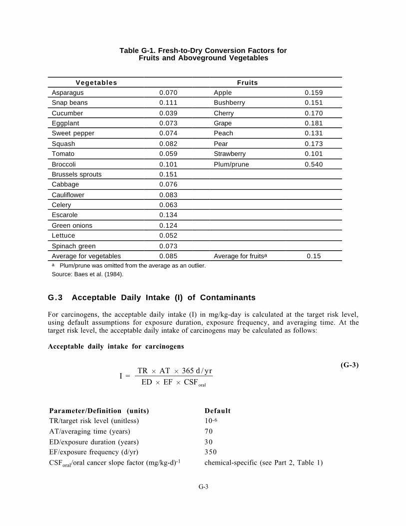
Table G-1. Fresh-to-Dry Conversion Factors forFruits and Aboveground Vegetables
Vegetables Fruits
Asparagus 0.070 Apple 0.159
Snap beans 0.111 Bushberry 0.151
Cucumber 0.039 Cherry 0.170
Eggplant 0.073 Grape 0.181
Sweet pepper 0.074 Peach 0.131
Squash 0.082 Pear 0.173
Tomato 0.059 Strawberry 0.101
Broccoli 0.101 Plum/prune 0.540
Brussels sprouts 0.151
Cabbage 0.076
Cauliflower 0.083
Celery 0.063
Escarole 0.134
Green onions 0.124
Lettuce 0.052
Spinach green 0.073
Average for vegetables 0.085 Average for fruitsa 0.15a Plum/prune was omitted from the average as an outlier.Source: Baes et al. (1984).
G.3 Acceptable Daily Intake (I) of Contaminants
For carcinogens, the acceptable daily intake (I) in mg/kg-day is calculated at the target risk level,using default assumptions for exposure duration, exposure frequency, and averaging time. At thetarget risk level, the acceptable daily intake of carcinogens may be calculated as follows:
Acceptable daily intake for carcinogens
I = TR H AT H 365 d / yr
ED H EF H CSForal
(G-3)
Parameter/Definition (units) DefaultTR/target risk level (unitless) 10-6
AT/averaging time (years) 70
ED/exposure duration (years) 30EF/exposure frequency (d/yr) 350
CSForal/oral cancer slope factor (mg/kg-d)-1 chemical-specific (see Part 2, Table 1)
G-3

For noncarcinogens, the acceptable daily intake (I) in mg/kg-day is calculated at a hazard quotient of1 using the following equation:
Acceptable daily intake (I) for noncarcinogens
I = HQ H RfD H AT H 365 d / yr
ED H EF
(G-4)
Parameter/Definition (units) DefaultHQ/target hazard quotient (unitless) 1
AT/averaging time (years) 30ED/exposure duration (years) 30
EF/exposure frequency (d/yr) 350
RfD/oral reference dose (mg/kg-d) chemical-specific (see Part 2, Table 1)
G.4 Contaminated Fraction (F) and Consumption Rate (CR)
Default values for the fraction of vegetables assumed to be contaminated (F) are recommended in theExposure Factors Handbook (U.S. EPA, 1990). For home gardeners, a high-end dietary fraction of0.40 is assumed for the ingestion of contaminated fruits and vegetables grown onsite.
The default values for total fruit and vegetable consumption rates (CR) cited in the Exposure FactorsHandbook are 0.140 and 0.2 kg/d fresh weight, respectively. Assuming that the homegrown fractionis roughly 0.25 to 0.40, EPA estimated fresh weight consumption rates of: (1) 0.088 kg/d ofaboveground unprotected fruits, (2) 0.076 kg/d of aboveground unprotected vegetables, and (3) 0.028kg/d of unprotected belowground vegetables (U.S. EPA, 1994). The consumption rates for fruits andvegetables are converted to dry weight based on the average fresh-to-dry conversion of 0.15 forfruits and 0.085 for vegetables presented in Table G-1. For unprotected belowground vegetables, theconsumption rate (CR) is calculated by multiplying the fresh weight consumption rate (0.028 kgFW/d) by the average conversion factor of 0.085 resulting in a CR of 0.0024 kg DW/d. Using thissame method, dry weight consumption rates of 0.0132 and 0.0065 kg DW/d were calculated forunprotected aboveground fruits and vegetables, respectively. Consequently, the overall consumptionrate (CR) for aboveground, unprotected fruits and vegetables is 0.0197 kg DW/d.
The distinction between protected and unprotected produce reflects evidence that, for protectedplants such as cantaloupe and citrus, there is very little translocation of contaminants to the edibleparts of the plant. EPA recognizes that, while these assumptions for contaminated fraction andconsumption rates are reasonable for general assessment purposes, there is likely to be widevariability on the types of produce grown at home, the percentage that is unprotected, and otherexposure-related characteristics (U.S. EPA, 1994). G.5 Soil-to-Plant Bioconcentration Factors (Br)
For metals, soil-to-plant bioconcentration factors (Br) for both aboveground and belowground plantsmust be identified from empirical studies because the relationship between soil concentration andplant concentration has not been described adequately to provide a mathematical construct for
G-4
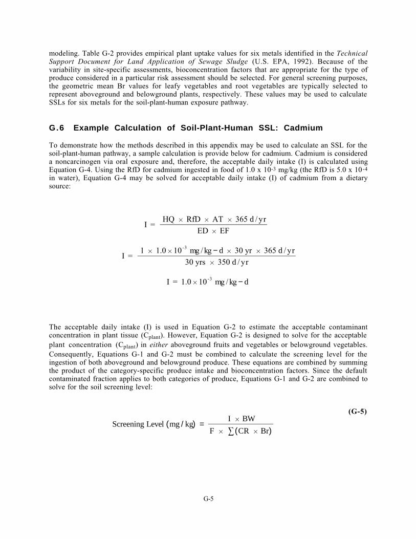
modeling. Table G-2 provides empirical plant uptake values for six metals identified in the TechnicalSupport Document for Land Application of Sewage Sludge (U.S. EPA, 1992). Because of thevariability in site-specific assessments, bioconcentration factors that are appropriate for the type ofproduce considered in a particular risk assessment should be selected. For general screening purposes,the geometric mean Br values for leafy vegetables and root vegetables are typically selected torepresent aboveground and belowground plants, respectively. These values may be used to calculateSSLs for six metals for the soil-plant-human exposure pathway.
G.6 Example Calculation of Soil-Plant-Human SSL: Cadmium
To demonstrate how the methods described in this appendix may be used to calculate an SSL for thesoil-plant-human pathway, a sample calculation is provide below for cadmium. Cadmium is considereda noncarcinogen via oral exposure and, therefore, the acceptable daily intake (I) is calculated usingEquation G-4. Using the RfD for cadmium ingested in food of 1.0 x 10⁻³ mg/kg (the RfD is 5.0 x 10⁻⁴
in water), Equation G-4 may be solved for acceptable daily intake (I) of cadmium from a dietarysource:
I = HQ H RfD H AT H 365 d / yr
ED H EF
I = 1 H 1 . 0 H 10- 3 mg / kg − d H 30 yr H 365 d / yr
30 yrs H 350 d / yr
I = 1 . 0 H 10- 3 mg / kg − d
The acceptable daily intake (I) is used in Equation G-2 to estimate the acceptable contaminantconcentration in plant tissue (Cplant). However, Equation G-2 is designed to solve for the acceptableplant concentration (Cplant) in either aboveground fruits and vegetables or belowground vegetables.Consequently, Equations G-1 and G-2 must be combined to calculate the screening level for theingestion of both aboveground and belowground produce. These equations are combined by summingthe product of the category-specific produce intake and bioconcentration factors. Since the defaultcontaminated fraction applies to both categories of produce, Equations G-1 and G-2 are combined tosolve for the soil screening level:
Screening Level ( mg / kg) = I H BW
F H 3 ( CR H Br)
(G-5)
G-5
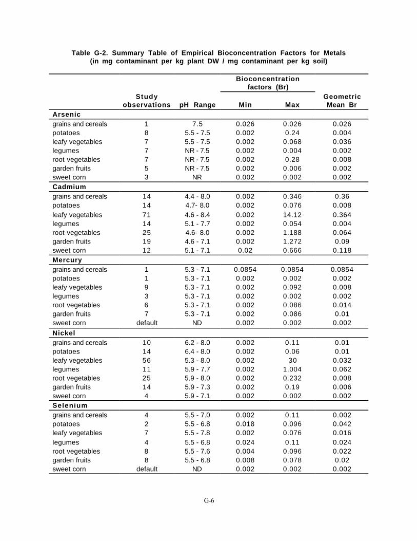
Table G-2. Summary Table of Empirical Bioconcentration Factors for Metals(in mg contaminant per kg plant DW / mg contaminant per kg soil)
Bioconcentrationfactors (Br)
Studyobservations pH Range Min Max
GeometricMean Br
Arsenicgrains and cereals 1 7.5 0.026 0.026 0.026potatoes 8 5.5 - 7.5 0.002 0.24 0.004leafy vegetables 7 5.5 - 7.5 0.002 0.068 0.036legumes 7 NR - 7.5 0.002 0.004 0.002root vegetables 7 NR - 7.5 0.002 0.28 0.008garden fruits 5 NR - 7.5 0.002 0.006 0.002sweet corn 3 NR 0.002 0.002 0.002Cadmiumgrains and cereals 14 4.4 - 8.0 0.002 0.346 0.36potatoes 14 4.7- 8.0 0.002 0.076 0.008leafy vegetables 71 4.6 - 8.4 0.002 14.12 0.364legumes 14 5.1 - 7.7 0.002 0.054 0.004root vegetables 25 4.6- 8.0 0.002 1.188 0.064garden fruits 19 4.6 - 7.1 0.002 1.272 0.09sweet corn 12 5.1 - 7.1 0.02 0.666 0.118Mercurygrains and cereals 1 5.3 - 7.1 0.0854 0.0854 0.0854potatoes 1 5.3 - 7.1 0.002 0.002 0.002leafy vegetables 9 5.3 - 7.1 0.002 0.092 0.008legumes 3 5.3 - 7.1 0.002 0.002 0.002root vegetables 6 5.3 - 7.1 0.002 0.086 0.014garden fruits 7 5.3 - 7.1 0.002 0.086 0.01sweet corn default ND 0.002 0.002 0.002
Nickelgrains and cereals 10 6.2 - 8.0 0.002 0.11 0.01potatoes 14 6.4 - 8.0 0.002 0.06 0.01leafy vegetables 56 5.3 - 8.0 0.002 30 0.032legumes 11 5.9 - 7.7 0.002 1.004 0.062root vegetables 25 5.9 - 8.0 0.002 0.232 0.008garden fruits 14 5.9 - 7.3 0.002 0.19 0.006sweet corn 4 5.9 - 7.1 0.002 0.002 0.002Seleniumgrains and cereals 4 5.5 - 7.0 0.002 0.11 0.002potatoes 2 5.5 - 6.8 0.018 0.096 0.042leafy vegetables 7 5.5 - 7.8 0.002 0.076 0.016legumes 4 5.5 - 6.8 0.024 0.11 0.024root vegetables 8 5.5 - 7.6 0.004 0.096 0.022garden fruits 8 5.5 - 6.8 0.008 0.078 0.02sweet corn default ND 0.002 0.002 0.002
G-6

Table G-2. (continued)
Bioconcentrationfactors (Br)
Studyobservations pH Range Min Max
GeometricMean Br
Zincgrains and cereals 13 5.3 - 8.0 0.016 0.368 0.1potatoes 14 4.7 - 8.0 0.01 0.122 0.024leafy vegetables 47 4.6 - 8.0 0.012 4.488 0.25legumes 10 5.1 - 7.7 0.002 0.11 0.036root vegetables 20 4.6 - 8.0 0.002 0.412 0.044garden fruits 21 4.6 - 7.3 0.002 0.394 0.046sweet corn 8 5.1 - 6.5 0.002 0.19 0.02NR = Not reportedND = No data
The input parameters in Equation G-5 correspond to input parameters in Equations G-1 and G-2,with a contaminated fraction (F) of 0.4, and consumption rates (CRag and CRb g) andbioconcentration factors (Brag and Brbg) specific to either aboveground or belowground produce.Solving Equation G-5 for cadmium using the default parameters in Equation G-2 for F, CRag, and CRbg
results in:
Screening Level = I H BW
0 . 4 H Σ ( CRag H Brag) + ( CRb g H Brb g)
Screening Level = 1 . 0 H 10- 3 mg / kg − d H 70 kg
0 . 4 H Σ ( 0 . 0197 H 0 . 364) + ( 0 . 0024 H 0 . 064) kg soil / d
Screening Level = 24 mg / kg soil
As described above, the geometric mean Br values for leafy vegetables and root vegetables wereselected to represent the bioconcentration factors (Br) for aboveground fruits and vegetables (Brag)and belowground vegetables (Brbg), respectively (see Table G-2). SSLs for the plant pathway that arecalculated using the bioconcentration factors for leafy and root vegetables are considered to begeneric SSLs by OERR. During site-specific assessments, OERR recommends that a weighted averagebioconcentration factor be used to reflect the type of produce grown and eaten locally.
G.7 Generic SSLs for Selected Metals
Table G-3 presents the generic SSLs for the soil-plant-human exposure pathway along with the SSLsfor direct soil ingestion. In addition, this table presents plant toxicity values identified in theToxicological Benchmarks for Screening Potential Contaminants of Concern for Effects onTerrestrial Plants: 1994 Revision (Will and Suter, 1994). The phytotoxicity values are either: (1) the
G-7

estimated 90th percentile of lowest observed effects concentrations (LOECs) from a data setconsisting of 10 or more values, or (2) the lowest LOEC from a data set with less than 10 values.The toxicological endpoints for the phytotoxicity were limited to growth and yield parametersbecause they are the most common endpoints reported in phytotoxicity studies and are ecologicallysignificant in terms of plant populations.
Table G-3. Comparison of Generic SSLs for Plant Pathway with the SSLs for SoilIngestion and LOEC Values for Phytotoxicity (all values in mg/kg)
Arsenic Cadmium Mercury Nickel Selenium Zinc
Generic plant SSL 0.4 24 270 5400 2400 10000
Soil ingestion SSL 0.4 78 23 1600 390 23000
Migration to groundwater SSLa
29(1) 8(0.4) 2(0.1) 130(7) 5(0.3) 12000(620)
Phytotoxicity LOEC 10 3 0.3 30 1 50a Values based on DAF of 20 (DAF of 1).
The comparison of the generic SSLs for the plant pathway with SSLs for soil ingestion and migrationto ground water suggests that this pathway may be of concern at sites contaminated with arsenic orcadmium. For mercury, nickel, and selenium, the generic plant SSLs are well above the SSLs based onsoil ingestion and migration to ground water. Thus, although SSLs based on these other pathways arelikely to be protective of the soil-plant-human pathway, other data suggest that phytotoxicity islikely to be the factor limiting exposure through plant uptake for these metals.
Phytotoxicity - The data in Table G-3 suggest that, for cadmium, mercury, nickel, and selenium,toxicity to plants will be observed at levels well below those estimated to elicit adverse effects inhumans. The phytotoxicity of arsenic, nickel, and zinc have been well documented. However, despitethe low phytotoxicity value for selenium, some authors have demonstrated that selenium canaccumulate in certain plants at high levels (Bitton et al., 1980). Moreover, many phytotoxicityvalues are based on a reduction in yield that may result in higher levels in the surviving produce.Thus, with the exception of zinc, phytotoxicity should not be used to rule out this exposure pathwayunless empirical data are available that are relevant to the site conditions (e.g., similar pH, organicmatter) and the type of crops likely to be grown.
Soil Characteristics - Because the majority of the plant uptake data for metals were generated insludge application studies, the empirical bioconcentration factors listed in Table G-2 may not beappropriate for use at all sites. For example, the adsorption "power" of sludge in the presence ofphosphates, manganese, hydrous oxides of iron, and Ca+2 may reduce the amount of metal that isbioavailable to plants. In addition, soil pH strongly influences the ability of plants to absorb metalsfrom soil. Several studies document that, as pH decreases, the bioavailability of many metalsincreases. In fact, agricultural practices maintain a soil pH of 5.5 or greater to protect againstaluminum and manganese phytotoxicity. However, 40 percent of the data evaluated for the SludgeRule were from studies in which the pH was less than 6, and, as a result, bioconcentration factors maybe artificially skewed.
Chemical Characteristics - Another factor that heavily influences plant uptake of metals is thechemical form of the metal. Researchers have observed that plant uptake rates of metal salts insludge tend to be higher than plant uptake rates in studies on elemental metals. Metal salts do not
G-8
adsorb to sludge the same way as “metals in nonsalt forms” and, consequently, they are morebioavailable to plants.
Type of produce - The bioconcentration potential of metals varies with plant type. As shown inTable G-2, the range of bioconcentration factors covers an order of magnitude for most metalsacross the seven categories of produce. Certain types of plants are resistant to some metals whilethese same metals may be highly toxic to other plant species. Depending on the type of crops grown,the generic soil-plant-human SSLs may not reflect the most appropriate measures ofbioconcentration.
Dietary habits - The dietary habits of the home gardener may result in an increase or decrease inexposure. The default values for consumption rate (CR) and contaminated fraction (F) representreasonably conservative estimates for these exposure parameters. However, individual consumersmay ingest significantly different quantities of produce and, depending on their fruit/vegetablepreferences, may rely on crops that are efficient accumulators of metals.
G.8 SSL Calculations for Organics Lacking Empirical Data
The lack of plant bioconcentration data on organics presented in the Technical Support Documentfor Land Application of Sewage Sludge (U.S. EPA, 1992) has been discussed in several other sources.For example, the status of empirical data on plant uptake and accumulation of organics was recentlyevaluated for a database on uptake/accumulation, translocation, adhesion, and biotransformation ofchemicals in plants (Nellessen and Fletcher, 1993). This database, referred to as UTAB, is one of themost comprehensive data sources available on chemical processes in plants and contains over 42,000records taken from more than 2,100 published papers. The authors found that, with the exception ofpesticides, uptake-response data for organic chemicals are available for roughly 25 percent of thechemicals monitored by EPA. Given the comprehensive nature of the UTAB database, modeling maybe the only alternative to evaluating the soil-plant-human pathway in the near future for manyorganic chemicals.
Recently, several authors have developed models to predict the uptake and accumulation of organicchemicals in plants (e.g., Matthies and Behrendt, 1994; McKone, 1994; Trapp et al., 1994). One ofthe most promising models for use as a risk assessment tool is PLANTX, a peer-reviewedpartitioning model that describes the dynamic uptake from soil, or solution, and the metabolism andaccumulation of xenobiotic chemicals in roots, stems, leaves, and fruits (Trapp et al., 1994). Unlikea number of other models used to estimate plant uptake, PLANTX is not based on regressionequations that correlate log Kow with plant bioconcentration; it is a mechanistic model that accountsfor major plant processes and requires only a few well-known input data. Moreover, it was designed asa risk assessment tool and has been validated for the herbicide bromicil and several nitrobenzenes. Afollow-on model (PLANTE) has recently been made available that also incorporates plant uptakeduring transpiration (i.e., accumulation directly from the air). The results on bromocil, nitrobenzene,etc., as well as ongoing validation studies suggest that the PLANT models may be a scientificallydefensible alternative to the uptake-response slopes generated by log Kow regressions.
G.9 Conclusions and Recommendations
The comparison of generic plant SSLs with generic SSLs for soil ingestion and migration to groundwater indicate that the soil-plant-human exposure pathway may be of concern for two of the sixmetals evaluated (arsenic and cadmium). For mercury, nickel, and selenium, SSLs based on the otherpathways are likely to be adequately protective of the soil-plant-human exposure pathway. Inaddition, data presented on the phytotoxicity of these metals and zinc suggest that toxic effects inplants are likely to be observed below levels that would be harmful to humans. Although this pathway
G-9

may not be of concern from a human health standpoint, these data suggest that metals could be ofparticular concern for ecological receptors.
Currently, EPA is developing methods to evaluate the uptake of organics into plants. In addition tothe efforts of the Office of Solid Waste and the Office of Research and Development mentioned inthe Introduction, OERR has jointly funded research on plant uptake of organics with the State ofCalifornia. These studies support ongoing revisions to the indirect, multimedia exposure model,CalTOX. Until these efforts are reviewed and finalized, OERR will continue to address the potentialfor plant uptake of organics on a case-by-case basis.
References
Bacci, Eros, and David Calamari. 1991. Air-to-leaf transfer of organic vapors to plants. In:Municipal Waste Incineration Risk Assessment. C.C. Travis editor, Plenum Press, New York.
Baes, C.F., R.D. Sharp, A.L. Sjoreen, and R.W. Shor. 1984. Review and Analysis of Parameters andAssessing Transport of Environmentally Released Radionuclides Through Agriculture. OakRidge National Laboratory, Oak Ridge, TN.
Bitton, G., B.L. Damron, G.T. Edds, and J.M. Davidson. 1980. Sludge -- Health Risks of LandApplication. Ann Arbor Science Publishers, Inc., Ann Arbor, MI.
Matthies, M., and H. Behrendt. 1994. Dynamics of leaching, uptake, and translocation: TheSimulation Model Network Atmosphere-plant-soil (SNAPS). In: Plant Contamination:Modeling and Simulation of Organic Chemical Processes. Stefan Trapp and J. Craig McFarlane eds, Lewis Publishers, Michigan.
McKone, T. 1994. Uncertainty and variability in human exposures to soil contaminants throughhomegrown food: a Monte carlo assessment. Risk Analysis 14 (4): 449-463.
McFarlane, Craig. 1991. Uptake of organic contaminants by plants. In: Municipal Waste IncinerationRisk Assessment. C.C. Travis editor, Plenum Press, New York.
Nellessen, J.E., and J.S. Fletcher. 1993. Assessment of published literature pertaining to theuptake/accumulation, translocation, adhesion and biotransformation of organic chemicals byvascular plants. Environmental Toxicology and Chemistry 12: 2045-2052.
Paterson, Sally and Donald Mackay. 1991. Current studies on human exposure to chemicals withemphasis on the plant route. In: Municipal Waste Incineration Risk Assessment. C.C. Traviseditor, Plenum Press, New York.
Trapp, S., and J.C. McFarlane. 1995. Plant Contamination. Modeling and Simulation of OrganicChemical Processes. Lewis Publishers, Boca Raton, FL.
Trapp, S., and J.C. McFarlane, and M. Matthies. 1994. Model for uptake of xenobiotic into plants:Validation with bromocil experiments. Environmental Toxicology and Chemistry 13 (3):413-422.
Travis, C.C., and A.D. Arms. 1988. Bioconcentration of organics in beef, milk and vegetation.Environmental Science and Technology 22(3):271-274.
G-10
U.S. EPA (Environmental Protection Agency). 1990. Exposure Factors Handbook. Office of Healthand Environmental Assessment, Exposure Assessment Group, Washington, DC. March.
U.S. EPA (Environmental Protection Agency). 1992. Technical Support Document for LandApplication of Sewage Sludge, Volume I and II. EPA 822/R-93-001a. Office of Water,Washington, DC.
U.S. EPA (Environmental Protection Agency). 1994. Estimating Exposure to Dioxin-likeCompounds. Volumes I-III: Site-specific Assessment Procedures. EPA/600/6-88/005C. Officeof Research and Development, Washington, DC. June.
Will, M.E. and G.W. Suter II. 1994. Toxicological Benchmarks for Screening PotentialContaminants of Concern for Effects on Terrestrial Plants: 1994 Revision . ES/ER/TM-85/R1.Prepared for the U.S. Department of Energy by the Environmental Sciences Division of theOak Ridge National Laboratory.
G-11

1
APPENDIX H
Evaluation of the Effect on the Draft SSLs of theJohnson and Ettinger Model (EQ, 1994a)

H-22
ENVIRONMENTAL QUALITY MANAGEMENT, INC.
MEMORANDUM
TO: Janine Dinan DATE: October 7, 1994
SUBJECT: Evaluation of the Effect on the Draft SSLs FROM: Craig S. Mannof the Johnson and Ettinger (1991) Modelfor the Intrusion of Contaminant VaporsInto Buildings
FILE: 5099-3 cc:
Under U.S. Environmental Protection Agency (EPA) Contract No. 68-D3-0035, Taskorder No. 0-25, Environmental Quality Management, Inc. (EQ) was directed to evaluate the effecton the draft soil screening levels (SSLs) of employing the Johnson and Ettinger (1991) model forestimating the intrusion rate of contaminant vapors from soil into buildings. This memorandumsummarizes the evaluation.
Model Review:
Johnson and Ettinger (1991 ) is a closed-form analytical solution for both convective anddiffusive transport of vapor-phase contaminants fully incorporated in soil into enclosed structures.The nondimensionalized mass balance is written as:
∂
∂µ C
t * -
L
L =
D L
k P L + i
i i*
p
D
*eff
p
v r Di i
*RΣ
∆Σ
∈
( ) ⋅ ( ) ⋅
∇ ∇ ∇ ∇* * * * * *P v vC C (1)
where * = Nondimensional variables
∈ i = Volume fraction of phase i, unitless
Ci = Concentration of contaminant in phase i, g/cm3
t = Time, s
LP = Convection path length, cm
LD = Diffusion path length, cm
P = Pressure in vapor-phase, g/cm-s2
∇ = Del operator, 1/cm
Cv = Contaminant concentration in vapor phase, g/cm3
Deff = Effective diffusion coefficient, cm2/s
µ = Vapor viscosity, g/cm-s

H-33
kv = Soil permeability to vapor flow, cm2
∆ Pr = Reference indoor-outdoor pressure differential, g/cm-s2
Ri = Formation rate of contaminant in phase i, g/cm3-s
and,
Ci* = Ci/Cr
∇ * = LD ∇
P* = P/∆Pr
t* = t (kv ∆ Pr/ LDLP µ)
Ri* =Ri LDLP µ /Crkr ∆ Pr
where Cr, LP and LD are characteristic concentration, convection pathway length, and diffusionpathway length, chosen to give the dependent concentration variable and derivatives of Ci* and P*magnitudes of order unity.
The mass balance solution includes the following assumptions:
1. The soil column is isotropic within any horizontal plane.
2. The effective diffusion coefficient is constant within any horizontal plane.
3. Concentration at the soil-air interface is zero (i.e., boundary layer resistance iszero).
4. No loss of contaminant occurs across the lower boundary (i.e., no leaching).
5. Source degradation and transformation are not considered.
6. Convective vapor flow near the building foundation is uniform.
7. Contaminant vapors enter the building primarily through openings in the walls andfoundation at or below grade.
8. Convective velocities decrease with increasing contaminant source-buildingdistance.
9. All contaminant vapors directly below a basement will enter the basement, unlessthe floor and walls are perfect vapor barriers.

H-44
10. The building contains no other contaminant sources or sinks, and the air volume iswell mixed.
Therefore,
Qbuilding Cbuilding = E (2)
where Qbuilding, Cbuilding, and E represent the volumetric flow rate or ventilation rate of the building(cm3/s), contaminant concentration within the building (g/cm3), and rate of contaminant entry (g/s),respectively.
Also,
α = Qbuilding/Csource (3)
where Csource is the vapor-phase contaminant concentration within the soil at the source, and αrepresents the attenuation coefficient. Csource is written as:
Csource = H C
+ K + Hs b
w d b a
ρρΘ Θ
(4)
where H = Henry's law constant, unitless
Cs = Soil bulk concentration, g/g
ρb = Soil dry bulk density, g/cm3
Θw = Soil water-filled porosity, unitless
Kd = Soil-water partion coefficient, cm3/g
Θa = Soil air-filled porosity, unitless.
The authors derive a solution for α for both steady-state conditions (i.e., depth of
contamination, z = ∞ ) and for quasi-steady-state conditions (0 < z < L). For steady-state
conditions α is written as:
α = D A
Q L exp
Q L
D A /
effB
building T
soil crackcrack
crack
x
exp exp Q L
D A +
D A
Q L +
D A
Q L
Q L
D A -1soil crack
crackcrack
effB
building T
effB
soil T
soil crackcrack
crack
(5)

H-55
where Deff = Effective diffusion coefficient, cm2/s
AB = Area of basement, cm2
LT = Source-building separation, cm
Qsoil = Volumetric flow rate of soil gas into the building, cm3/s
LCrack = Building foundation thickness, cm
DCrack = Effective diffusion coefficient through crack, cm2/s (DCrack = Deff)
ACrack = Area of crack, cm2
Qbuilding = Building ventilation rate, cm3/s.
For quasi-steady-state conditions the long-term average attenuation coefficient <a> is:
< >
( )[ ]α ρτ
β τ β = C H A
C L
H + 2 - b R C B
source
T0
C
2∆∆
ΨQbuilding
1 2/(6)
where ρb = Soil dry bulk density, g/cm3
CR = Average contaminant level in soil, g/g
∆Hc = Thickness of depth over which contaminant is distributed, cm
AB = Area of basement, cm2
Qbuilding = Building ventilation rate, cm3/s
Csource = Vapor-phase soil concentration at source, g/cm3
τ = Exposure averaging period, s
LT0 = Source-building separation at t=0, cm
and,
β = D A
L Q1 - exp
Q L
A + 1
effB
T0
soil
soil crack
crack
−
Dcrack (7)
Ψ = D C / L Ceffsource T
0b R( )2 ρ (8)

H-66
The time required to deplete a finite source (τ D) of depth ∆Hc is given as:
τ β βD =
H / L + -
2 C T
0 2[ ]∆Ψ
(9)
If the exposure period (τ) is greater than τD, the average emission rate into the building <E> isgiven as a simple mass balance:
<E> = ρb CR ∆HC AB / τ (10)
and the average building concentration (Cbuilding) is:
Cbuilding = <E>/Qbuilding (11)
Evaluation
In order to evaluate the effects of using the model on the SSLs for volatile contaminants, acase example was constructed which best estimates a reasonable high end exposure pointconcentration for residential land use. Where possible, values of model variables were takendirectly from Johnson and Ettinger (1991).
The case example assumes that a residential dwelling with a basement is constructed withinthe area of homogeneous residual contamination such that the contaminant source lies directlybelow the basement floor at t = 0. Therefore, the diffusion and convection path lengths were setequal to the thickness of the basement slab (15 cm). Soil permeability to vapor flow from thebasement floor to the bottom of contamination was set equal to 1.0 x 10⁻⁸ cm2 (1 darcy) which isrepresentative of silty to fine sand. Soil column-building pressure differential was set equal to 1pascal (10g/cm-s2) as a reasonable long-term average value (Johnson and Ettinger, 1991). Valuesfor all other soil properties were set equal to those of the Generic SSLs in the July 1994 TechnicalBackground Document for Draft Soil Screening Level Framework (TBD). Building variables, i.e.,basement area, ventilation rate, etc., were taken from Johnson and Ettinger (1991).
In the analysis, the values for Cbuilding (kg/m3) were calculated for the 42 chemicals in theTBD for which human health benchmarks are available. Please note that the values of Csource andCbuilding were calculated for an initial soil concentration of 1 mg/kg instead of 1 x 10⁻⁶ g/g. This wasdone to facilitate reverse calculation of the SSL in units of mg/kg. Therefore, these values areartificially high by a factor of 1 x 10⁶. The inverse of the value of Cbuilding (m
3/kg) was used as theindoor volatilization factor (VFindoor) and substituted into Equations 2-4 or 2-5 of the TBD asappropriate to calculate the resulting carcinogenic and noncarcinogenic inhalation SSLs. SSLs werecalculated for both steadystate conditions (infinite source depth) and quasi-steady-state conditions(finite source depth). In each case were the exposure period exceeded the time required for sourcedepletion (finite source depth), the volatilization factor was normalized to an average contaminantlevel in soil (Cr) of 1 mg/kg. For quasi-steady-state conditions, the depth to the bottom ofcontamination was set equal to 2 meters below the basement floor.
The value of the indoor SSL for each contaminant was compared to the respective SSLcalculated for outdoor exposures of the same duration using the Generic SSL calculations found inthe TBD. The outdoor SSLs were computed for a 30 acre square area source of emissions. Table 1summarizes the results of this comparison. The attachment to this memorandum gives the detailedcomputations for this evaluation.

H-77
TABLE 1.SUMMARY OF INDOOR AND OUTDOOR INHALATION SSLs FOR
VOLATILE CONTAMINANTS
ChemicalIndoor SSL,
infinite source(mg/kg)
Indoor SSL,finite source
(mg/kg)
Outdoor SSL,infinite source
(mg/kg)
Aldrin 0.4 0.4 0.5Benzene 0.002 0.02 0.5Bis(2-chloroethyl)ether 0.02 0.05 0.3Bromoform 0.8 0.9 43Carbon disulfide 0.03 0 7 11Carbon tetrachloride 0.0007 0.01 0.2Chlordane 51 53 54Chlorobenzene 0.7 2 87Chloroform 0.001 0.007 0.2DDT 5a 5 a 5a
1,2-Dichlorobenzene 26 65 297a
1,4-Dichlorobenzene 102 235 a 235a
1,1-Dichloroethane 4 35 9391,2-Dichloroethane 0.002 0.007 0.31,1-Dichloroethylene 0.0001 0.003 0.041,2-Dichloropropane 0.06 0.3 101,3-Dichloropropene 0.0007 0.004 0.1Dieldrin 3 4 2Ethylbenzene 21 69 257 a
Heptachlor 0.04 0.04 0.3Heptachlor epoxide 1 1 1Hexachloro-1,3-butadiene 0.03 0.05 1Hexachlorobenzene 0.3 0.6 1HCH-alpha(alpha-BHC) 0.5 0.6 0.9HCH-beta(beta-BHC) 7 a 7 a 7 a
Hexachlorocyclopentadiene 0.06 0.07 2Hexachloroethane 0.6 0.6 45Methyl bromide 0.01 0.3 3Methylene chloride 0.04 0.3 7Nitrobenzene 9 25 100Styrene 185 472 1439 a
1,1,2,2-Tetrachloroethane 0.007 0.02 0.4Tetrachloroethylene 0.05 0.3 11Toluene 6 28 521 a
Toxaphene 2 2 2 a
1,2,4-Trichlorobenzene 6 9 2141,1,1-Trichloroethane 5 69 980 a
1,1,2-Trichloroethane 0.009 0.02 1Trichloroethylene 0.01 0.09 32,4,6-Trichlorophenol 64 94 190Vinyl acetate 5 14 351Vinyl chloride 0.00002 0.002 0.01
a = SSL based on Csat

H-88
As can be seen from Table 1, results on a chemical-specific basis indicate a rate of changeas high as three orders of magnitude between the outdoor SSL and the infinite source indoor SSLsin the case of highly volatile contaminants. For very persistent contaminants, the relative differencewas considerably less, and in some cases there was no difference in SSL concentrations.
This variability is due to: 1) the variability in the human health benchmarks used to calculatethe risk-based SSLs, and 2) the apparent diffusion coefficient of each compound. The apparentdiffusion coefficient can be expressed as the effective diffusion coefficient through soil divided bythe liquid-phase partition coefficient (Jury et al., 1983). The apparent diffusion coefficient (DA) isgiven here so as not to be confused with the effective diffusion coefficient (Deff) from Johnson andEttinger (1991):
DA Hb w a = D H + D K + + a
10/3a w
10/3w t
2dΘ Θ Θ Θ Θ( )[ ]/ /( )ρ (12)
where DA = Apparent diffusion coefficient, cm2/s
Θa = Air-filled soil porosity, unitless
Da = Diffusivity in air, cm2/s
H = Henry's law constant, unitless
Θw = Water-filled soil porosity, unitless
Dw = Diffusivity in water, cm2/s
Θt = Total soil porosity, unitless
ρb = Soil dry bulk density, g/cm3
Kd = Soil-water partition coefficient, cm3/g.
With all nonchemical-specific variables held constant, Figure 1 shows the exponentialrelationship between the apparent diffusion coefficient and the building concentration for quasi-steady-state conditions (finite source).
For nonchemical-specific variables, a sensitivity analysis was performed for soilpermeability to vapor flow (kv), soil-building pressure differential (∆ P), depth of contamination
(∆Hc), source-building separation at t = 0 (LT0), crack-to-total area ratio (η), and building
ventilation rate (Qbuilding).

H-99
Figure 1Building Concentration Versus Apparent Diffusion Coefficient

H-101 0
Table 2 shows the results of the sensitivity analysis for the quasi-steady-state condition(finite source). As can be seen from Table 2, the effect of the building ventilation rate is linear if thevalue of Csat is not included in limiting the value of the SSL. Depth of contamination (∆Hc) has thegreatest effect for contaminants with higher apparent diffusion coefficients (e.g., benzene,chloroform, vinyl chloride, etc.), in that as ∆Hc increases, the time required for source depletion
(τD) also increases. Therefore, with greater initial contaminant mass in the soil, these compoundsare emitted for a longer period of time thus reducing the SSL. For the more persistentcontaminants, an increase in kv or ∆P produces the greatest results. This is to be expected as values
of τD for these contaminants exceed the exposure duration. Table 2 also indicates that an order of
magnitude change in values Of LT0 and η produce same order of magnitude results. It must be
remembered, however, that in the case of LT0, the model assumes isotropic soil conditions from the
point of building entry to the bottom of contamination. As LT0 increases, α decreases until
diffusion not convection limits the rate of contaminant vapor transport. The effect of changes in thevalue of η decrease as values of kv decrease such that for very permeable soils andconvection-dominated vapor transport, the effect of crack size is relatively insignificant.
Conclusions
Use of the Johnson and Ettinger (1991) model to calculate SSLs based on indoor chronicexposures can have significant impacts on the values of the SSLs for contaminants with highapparent diffusion coefficients. When comparing the infinite source indoor model to the infinitesource outdoor model for these contaminants, values of the SSL differ by orders of magnitude forcase example conditions. Under these conditions, diffusion is the limiting transport mechanismsfor all but one contaminant for both steady-state and quasi-steady-state conditions. To effect caseexample conditions, the following must be true:
1. The contaminant source must be relatively close or directly beneath the structure.
2. The soil between the structure and the source must be very permeable (kv, ≥ 10-8
cm2).
3. The structure must be underpressurized.
4. The air within the structure must be well mixed (i.e., little or no soil-air boundarylayer resistance).
5. The combination of diffusion coefficient through the cracks, area of the cracks, andbuilding underpressurization must offer no more resistance than the soil columnbeneath the structure.
From this evaluation, the four most important factors affecting the average long-termbuilding concentration and thus the SSL are building ventilation rate, source-building separation,soil permeability to vapor flow, and source depth. If the source of contamination is relatively deepand close to the building, and if the soil between the source and the building is very permeable,building concentrations of contaminants with relatively high apparent diffusion coefficients willincrease dramatically.

H-111 1
TABLE 2.MODEL SENSITIVITY TO NONCHEMICAL SPECIFIC VARIABLES
Ratio of Variable-to-Test Condition SSL
Apparentdiffusion
coefficient,DA
Testcondition
SSL,Soil vapor
permeability,
Soil-bldg.pressure
differential,
Depth tosourcelower
boundary,
Source-bldg.
separationat t=0,
Inverse ofcrack-to-total area
ratio,
Bldg.ventilation
rate,Chemical (cm2/s) (mg/kg) kv x 10 ∆P x 10 ∆Hc x 10 LT
0 x 10 1/η x 10 Qbuilding x 10
DDT 1.16E-09 5a 1 1 1 1 1 1.0Dieldrin 1.59E-09 4 0.1 0.1 1 1.2 1.5 3.4HCH-beta(beta-BHC) 3.54E-09 7a 0.8 0.8 1 1 1 1.0Chlordane 5.63E-09 53 0.1 0.1 1 1.3 1.3 1.3Heptachlor epoxide 5 78E-09 1 0.1 0.1 1 1.3 1.5 8.4Aldrin 1.03E-08 0.4 0.1 0.1 1 1.2 1.5 10HCH-alpha(alpha-BHC) 2.81E-08 0.6 0.1 0.1 1 1.2 1.5 10Toxaphene 3.69E-08 2 0.1 0.1 1 1.1 1.1 1.12,4,6-Trichlorophenol 1.81E-07 94 0.1 0.1 1 1.1 1.5 10Hexachlorobenzene 284E-07 0.6 0.1 0.1 1 1.1 1.5 3.2Heptachlor 3.52E-07 0.04 0.1 0.1 1 1.3 1.5 10Hexachloroethane 1.80E-06 0.6 0.3 0.3 1 2 1.4 10Nitrobenzene 3.92E-06 25 0.1 0.1 1 1 1.5 10Bis(2-chloroethyl)ether 5.94E-06 0.05 0.1 0.1 1 1 1.5 10Hexachlorocyclo-pentadiene 1.06E-05 0.07 0.2 0.2 1 1.2 1.5 101,2,4-Trichlorobenzene 1.89E-05 9 0.1 0.1 1 1.1 1.5 10Bromoform 2.32E-05 0.9 0.2 0.2 1 1.2 1.5 10Hexachloro-1,3-butadiene 6.97E-05 0.05 0.1 0.1 1 1.1 1.5 10Styrene 9.50E-05 472 0.1 0.1 1 1 1 5 3.01,1,2,2-Tetrachloroethane 9.89E-05 0.02 0.2 0 2 1 1 1 5 101,2-Dichlorobenzene 1.34E-04 65 0.2 0.2 1 1 1.5 4.51,4-Dichlorobenzene 1.38E-04 235a 0.2 0.2 1 1 1 1.01,1,2-Trichloroethane 3.04E-04 0.02 0.4 0.4 1 1 1.5 10Chlorobenzene 5.18E-04 2 0.8 0.8 1 1 1.5 10Vinyl acetate 7.79E-04 14 1 1 1 1 1.5 101,2-Dichloropropane 8.57E-04 0.007 0.9 0.9 1 1 1.5 10Ethylbenzene 8.64E-04 69 1 1 0.8 1 1.2 3.71,2-Dichbropropane 1.24E-03 0.3 1 1 0.6 1 1 10Toluene 1.25E-03 28 1 1 0.7 1 1 10Tetrachloroethylene 1.34E-03 0.3 1 1 0.5 1 1 101,3-Dichloropropene 1.44E-03 0.004 1 1 0.4 1 1 10Chloroform 1.91E-03 0.007 1 1 0.5 1 1 101,1-Dichloroethane 2.08E-03 35 1 1 0.4 1 1 10Benzene 2.12E-03 0.02 1 1 0.4 1 1 10Trichloroethylene 2.44E-03 0.09 1 1 0.3 1 1 10Methylene chloride 2.45E-03 0.3 1 1 0.4 1 1 101,1,1-Trichioroethane 3.79E-03 69 1 1 0.2 1 1 10Carbon tetrachloride 3.82E-03 0.01 1 1 0.2 1 1 10Carbon disulfide 5.67E-03 0.7 1 1 0.2 1 1 101,1-Dichloroethylene 7.09E-03 0.003 1 1 0.1 1 1 10Methyl bromide 8.56E-03 0.3 1 1 0.1 1 1 10Vinyl chloride 2.40E-02 0.002 1 1 0.1 1 1 10
a = SSL based Csat

H-121 2
It should be noted, however, that soil permeability, kV, is the most variable parameter atany given site, and may vary by three orders of magnitude across a typical residential lot (Johnsonand Ettinger, 1991). For this reason, the overall effective diffusion coefficient should bedetermined by integration across each soil type. Overall diffusion/convection vapor transport willtherefore be limited by the soil stratum offering the greatest resistance to vapor flow.
References
Johnson, Paul C., and Robert A. Ettinger. 1991. Heuristic model for predicting the intrusion rateof contaminant vapors into buildings. Environ. Sci. Technol., 25(8):1445-1452.
Jury, W. A., W. J. Farmer, and W. F. Spencer. 1983. Behavior Assessment Model for TraceOrganics in Soil, l, Model description. J. Environ. Qual., 12:558-564.
Attachment

H-131 3
ATTACHMENT
DETAILED MODEL EVALUATION

H-141 4
COMPARISON OF INDOOR AND OUTDOOR INHALATION SSLs FOR VOLATILE CONTAMINANTS
Soil bulkdensity,
Soilmoisture,
Soilmoisutre,
Soil totalporosity,
Soil air-filled
porosity,
Soilwater-filled
porosity,Diffusivity
in air,Diffusity in
water,
Effectivediffusioncoeffi-cient,
Soil vaporpermea-
bility,
Soil-bldg.pressuredifferen-
tial
Diffusionpath
length,
Convec-tion pathlength,
Vaporviscosity,
Pecletnumber,
Henry’slaw
constant,
Organiccarbonpartitioncoeffi-cient,
ρb w Θwη Θa Θw Da Dw Do Kv ∆P Ld Lp
µ Pe H Koc
Chemical CAS No. (g/cm3) (g/g) (cm3/cm3) (unitless) (unitless) (unitless) (cm2/s) (cm2/s) (cm2/s) (cm3) (g/cm-s2) (cm) (cm) (g/cm-s) (unitless) (unitless) (cm3/g)
Aldrin 309-00-2 1.5 0.1 0.15 0.434 0.284 0.150 1.32E-02 4.86E-06 1.05E-03 1.00E-08 10 15 15 1.80E-04 0.53 4.20E-03 4.84E+04Benzene 71-43-2 1.5 0.1 0.15 0.434 0.284 0.150 8.70E 02 9.80E-066 6.95E-03 1.00E-08 10 15 15 1.80E-04 0.08 2.20E-01 5.70E+01Bis(2-chloroethyl)ether 111-44-4 1.5 0.1 0.15 0.434 0.284 0.150 6.92E-02 7.53E-06 5.53E-03 1.00E-08 10 15 15 1.80E-04 0.10 8.80E-04 7.60E+01Bromoform 75-25-2 1.5 0.1 0.15 0.434 0.284 0.150 1.49E-02 1.03E-05 1.19E-03 1.00E-08 10 15 15 1.80E-04 0.47 2.50E-02 1.26E+02Carbon disulfide 75-15-0 1.5 0.1 0.15 0.434 0.284 0.150 1.04E-01 1.00E-05 8.31E-03 1.00E-08 10 15 15 1.80E-04 0.07 5.20E-01 5.20E+01Carbon tetrachloride 56-23-5 1.5 0.1 0.15 0.434 0.284 0.150 7.80E-02 8.80E-06 6.23E-03 1.00E-08 10 15 15 1.80E-04 0.09 1.20E+00 1.64E+02Chlordane 57-74-9 1.5 0.1 0.15 0.434 0.284 0.150 1.18E-02 4.37E-06 9.43E-04 1.00E-08 10 15 15 1.80E-04 0.59 2.70E-03 5.13E+04Chlorobenzene 108-90-7 1.5 0.1 0.15 0.434 0.284 0.150 7.30E-02 8.70E-06 5.83E-03 1.00E-08 10 15 15 1.80E-04 0.10 1.80E-01 2.04E+02Chloroform 67-66-03 1.5 0.1 0.15 0.434 0.284 0.150 1.04E-01 1.00E-05 8.31E-03 1.00E-08 10 15 15 1.80E-04 0.07 1.60E-01 5.60E+01DDT 50-29-3 1.5 0.1 0.15 0.434 0.284 0.150 1.37E-02 4.95E-06 1.09E-03 1.00E-08 10 15 15 1.80E-04 0.51 2.20E43 2.37E+051,2-Dichlorobenzene 95-50-1 1.5 0.1 0.15 0.434 0.284 0.150 6.90E-02 7.90E-06 5.51E-03 1.00E-08 10 15 15 1.00E-04 0.10 8.60E-02 3.76E+021,4-Dichlorobenzene 106-46-7 1.5 0.1 0.15 0.434 0.284 0.150 6.90E-02 7.90E-06 5.51E-03 1.00E-08 10 15 15 1.80E-04 0.10 1.20E-01 5.16E+021,1-Dichloroethane 75-34-3 1.5 0.1 0.15 0.434 0.284 0.150 7.42E-02 1.04E-05 5.93E-03 1.00E-08 10 15 15 1.80E-04 0.09 2.40E41 5.20E+011,2-Dichloroethane 107-06-2 1.5 0.1 0.15 0.434 0.284 0.150 1.04E-01 9.90E-06 8.31E-03 1.00E-08 10 15 15 1.80E-04 0.07 5.20E-02 3.80E+011,1-Dichloroethylene 75-35 -4 1.5 0.1 0.15 0.434 0.284 0.150 9.00E-02 1.04E-05 7.19E-03 1.00E-08 10 15 15 1.80E-04 0.08 1.00E+00 6.50E+011,2-Dichloropropane 78-87-5 1.5 0.1 0.15 0.434 0.284 0.150 7.82E-02 8.73E-06 6.25E-03 1.00E-08 10 15 15 1.80E-04 0.09 1.20E-01 4.70E+011,3-Dichloropropene 542-75-6 1.5 0.1 0.15 0.434 0.284 0.150 6.26E-02 1.00E-05 5.00E-03 1.00E-08 10 15 15 1.80E-04 0.11 1.20E-01 2.60E+01Dieldrin 60-57-1 1.5 0.1 0.15 0.434 0.284 0.150 1.25E-02 4.74E4-6 9.99E-04 1.00E-08 10 15 15 1.80E-04 0.56 1.10E-04 1.09E+04Ethylbenzene 100-41-4 1.5 0.1 0.15 0.434 0.284 0.150 7.50E-02 7.80E-06 5.99E-03 1.00E-08 10 15 15 1.80E-04 0.09 3.20E-01 2.21E+02Heptachlor 76-44-8 1.5 0.1 0.15 0.434 0.284 0.150 1.12E-02 5.69E-06 8.95E-04 1.00E-08 10 15 15 1.80E-04 0.62 2.40E-02 6.81E+03Heptachlor epoxide 1024-57-3 1.5 0.1 0.15 0.434 0.284 0.150 1.22E-02 4.68E-06 9.75E-04 1.00E-08 10 15 15 1.80E-04 0.57 3.40E-04 7.24E+03Hexachloro-1,3-butadiene 87-68-3 1.5 0.1 0.15 0.434 0.284 0.150 5.61E-02 6.16E-06 4.48E-03 1.00E-08 10 15 15 1.80E-04 0.12 9.80E-01 6.99E+03Hexachlorobenzene 118-74-1 1.5 0.1 0.15 0.434 0.284 0.150 5.42E-02 5.91E-06 4.33E-03 1.00E-08 10 15 15 1.80E-04 0.13 220E-02 3.75E+04HCH-alpha(alpha-BHC) 319-84-6 1.5 0.1 0.15 0.434 0.284 0.150 1.76E-02 5.57E-06 1.41E-03 1.00E-08 10 15 15 1.80E-04 0.39 2.80E-04 1.76E+03HCH-beta(beta-BHC) 319-85-7 1.5 0.1 0.15 0.434 0.284 0.150 1.76E-02 5.57E-06 1.41E-03 1.00E-08 10 15 15 1.80E-04 0.39 1.40E-05 2.28E+03Hexachlorocyclopentadiene 77-47-4 1.5 0.1 0.15 0.434 0.284 0.150 1.61E-02 7.21E-06 1.29E-03 1.00E-08 10 15 15 1.80E-04 0.43 7.10E-01 9.59E+03Hexachloroethane 67-72-1 1.5 0.1 0.15 0.434 0.284 0.150 2.49E-03 6.80E-06 1.99E-04 1.00E-08 10 15 15 1.80E-04 2.79 1.50E-01 1.83E+03Methyl bromide 74-83-9 1.5 0.1 0.15 0.434 0.284 0.150 7.28E-02 1.21E-05 5.82E-03 1.00E-08 10 15 15 1.80E-04 0.10 5.80E-01 9.00E+00Methylene chloride 75-09-2 1.5 0.1 0.15 0.434 0.284 0.150 1.01E-01 1.17E-05 8.07E-03 1.00E-08 10 15 15 1.80E-04 0.07 9.70E-02 1.60E+01Nitrobenzene 98-95-3 1.5 0.1 0.15 0.434 0.284 0.150 7.60E-02 8.60E-06 6.07E-03 1.00E-08 10 15 15 1.80E-04 0.09 8.40E-04 1.31E+02Styrene 100-42-5 1.5 0.1 0.15 0.434 0.284 0.150 7.10E-02 8.00E-06 5.67E-03 1.00E-08 10 15 15 1.80E-04 0.10 1.40E-01 9.12E+021,1,2,2-Tetrachloroethane 79-34-5 1.5 0.1 0.15 0.434 0.284 0.150 7.10E-02 7.90E-06 5.67E-03 1.00E-08 10 15 15 1.80E-04 0.10 1.50E-02 7.90E+01Tetrachloroethylene 127-18-4 1.5 0.1 0.15 0.434 0.284 0.150 7.20E-02 8.20E-06 5.75E-03 1.00E-08 10 15 15 1.80E-04 0.10 7.10E-01 3.00E+02Toluene 108-88-3 1.5 0.1 0.15 0.434 0.284 0.150 8.70E-02 8.60E-06 6.95E-03 1.00E-08 10 15 15 1.80E-04 0.08 2.50E-01 1.31E+02Toxaphene 8001-35-2 1.5 0.1 0.15 0.434 0.284 0.150 1.16E-02 4.34E-06 9.27E-04 1.00E-08 10 15 15 1.80E-04 0.60 1.40E-04 5.01E+021,2,4-Trichlorobenzene 120-82-1 1.5 0.1 0.15 0.434 0.284 0.150 3.00E-02 8.23E-06 2.40E-03 1.00E-08 10 15 15 1.80E-04 0.23 1.10E-01 1.54E+031,1,1-Trichloroethane 71-55-6 1.5 0.1 0.15 0.434 0.284 0.150 7.80E-02 8.80E-06 6.23E-03 1.00E-08 10 15 15 1.80E-04 0.09 7.60E-01 9.90E+011,1,2-Trichloroethane 79-00-5 1.5 0.1 0.15 0.434 0.284 0.150 7.80E-02 8.80E-06 6.23E-03 1.00E-08 10 15 15 1.80E-04 0. 09 4.10E-02 7.60E+01Trichloroethylene 79-01-6 1.5 0.1 0.15 0.434 0.284 0.150 7.90E-02 9.10E-06 6.31E-03 1.00E-08 10 15 15 1.80E-04 0.09 4.30E-01 9.40E+012,4,6-Trichlorophenol 88-06-2 1.5 0.1 0.15 0.434 0.284 0.150 3.14E-02 6.36E-06 2.51E-03 1.00E-08 10 15 15 1.80E-04 0.22 1.70E-04 2.83E+02Vinyl acetate 108-05-4 1.5 0.1 0.15 0.434 0.284 0.150 8.50E-02 9.20E-06 6.79E-03 1.00E-08 10 15 15 1.80E-04 0.08 2.30E-02 5.00E+00Vinyl chloride 75-01-4 1.5 0.1 0.15 0.434 0.284 0.150 1.06E-01 1.23E-05 8.47E-03 1 00E-08 10 15 15 1.80E-04 0.07 3.50E+00 1.10E+01
NA = not appilcablea = SSL based on Csat

H-151 5
COMPARISON OF INDOOR AND OUTDOOR INHALATION SSLs FOR VOLATILE CONTAMINANTS
Soilorganiccarbon
fraction,
Soil-waterpartition
coefficientInitial soil
conc.,
Sourcevaporconc.,
Floor-wallseam
perimeter,
Crackdepthbelowgrade,
Crackradius,
Averagevapor
flow rateintobldg.
Source-bldg.
separationat t=0,
Area ofbase-ment,
Bldg.foundation
thick-nesses,
Crackeffectivediffusioncoeffi-cient,
Crack-to-total
areaArea ofcrack,
Buiildingventilation
rate,
Depth tosourcelower
boundary,Exposureduration,
fo c K4 Cr Csource X crack Z crack rcrack Q soi l Lto Indoor As Lcrack Dcrack ratio, A crack Indoor Q building ∆Hc
τ
Chemical (unitless) (cm3/g) (mg/kg) (g/cm3) (cm) (cm) (cm) (cm3/s) (cm) ψ (cm2) (cm) (cm2/s) η (cm2) β (cm3/s) (cm) (sec)
Aldrin 0.006 2.90E+02 1.00E+00 1.45E-05 3400 200 4.06 2.59 15 4.52E-11 1.38E+06 15 1.05E-03 0.01 1.38E+04 3.85E+01 2.90E+04 200 9.46E+08
Benzene 0.006 3.42E-01 1.00E+00 4.55E-01 3400 200 4.06 2.59 15 9.37E-06 1.38E+06 15 6.95E-03 0.01 1.38E+04 2.48E+02 2.90E+04 200 9.46E+08
Bis(2-chloroethyl)ether 0.006 4.56E-01 1.00E+00 1.58E-03 3400 200 4.06 2.59 15 2.59E-08 1.38E+06 15 5.53E-03 0.01 1.38E+04 1.98E+02 2.90E+04 200 9.46E+08
Bromoform 0.006 7.56E-01 1.00E+00 2.90E-02 3400 200 4.06 2.59 15 1.02E-07 1.38E+06 15 1.19E-03 0.01 1.38E+04 4.34E+01 2.90E+04 200 9.46E+08
Carbon disulfide 0.006 3.12E-01 1.00E+00 1.02E+00 3400 200 4.06 2.59 15 2.51E-05 1.38E+06 15 8.31E-03 0.01 1.38E+04 2.97E+02 2.90E+04 200 9.46E+08
Carbon tetrachloride 0.006 9.84E-01 1.00E+00 9.15E-01 3400 200 4.06 2.59 15 1.69E-05 1.38E+06 15 6.23E-03 0.01 1.38E+04 2.23E+02 2.90E+04 200 9.46E+08
Chlordane 0.006 3.08E+02 1.00E+00 8.77E-06 3400 200 4.06 2.59 15 2.45E-11 1.38E+06 15 9.43E-04 0.01 1.38E+04 3.46E+01 2.90E+04 200 9.46E+08
Chlorobenzene 0.006 1.22E+00 1.00E+00 1.33E-01 3400 200 4.06 2.59 15 2.29E-06 1.38E+06 15 5.83E-03 0.01 1.38E+04 2.09E+02 2.90E+04 200 9.46E+08
Chloroform 0.005 3.36E-01 1.00E+00 3.43E-01 3400 200 4.06 2.59 15 8.45E-06 1.38E+06 15 8.31E-03 0.01 1.38E+04 2.97E+02 2.90E+04 200 9.46E+08
DDT 0.006 1.42E+03 1.00E+00 1.55E-06 3400 200 4.06 2.59 15 5.02E-12 1.38E+06 15 1.09E-03 0.01 1.38E+04 4.00E+01 2.90E+04 200 9.46E+08
1,2-Dichlorobenzene 0.006 2.26E+00 1.00E+00 3.63E-02 3400 200 4.06 2.59 15 5.92E-07 1.38E+06 15 5.51E-03 0.01 1.38E+04 1.97E+02 2.90E+04 200 9.46E+08
1,4-Dichlorobenzene 0.006 3.10E+00 1.00E+00 3.73E-02 3400 200 4.06 2.59 15 6.09E-07 1.38E+06 15 5.51E-03 0.01 1.38E+04 1.97E+02 2.90E+04 200 9.46E+08
1,1-Dichloroethane 0.006 3.12E-01 1.00E+00 5.25E-01 3400 200 4.06 2.59 15 9.22E-06 1.38E+06 15 5.93E-03 0.01 1.38E+04 2.12E+02 2.90E+04 200 9.46E+08
1,2-Dichloroethane 0.006 2.28E-01 1.00E+00 1.54E-01 3400 200 4.06 2.59 15 3.79E-06 1.38E+06 15 8.31E-03 0.01 1.38E+04 2.97E+02 2.90E+04 200 9.46E+08
1,1-Dichloroethylene 0.006 3.90E-01 1.00E+00 1.47E+00 3400 200 4.06 2.59 15 3.14E-05 1.38E+06 15 7.19E-03 0.01 1.38E+04 2.57E+02 2.90E+04 200 9.46E+08
1,2-Dichloropropane 0.006 2.82E-01 1.00E+00 2.97E-01 3400 200 4.06 2.59 15 5.49E-06 1.38E+06 15 6.25E-03 0.01 1.38E+04 2.23E+02 2.90E+04 200 9.46E+08
1,3-Dichloropropene 0.006 1.56E-01 1.00E+00 4.31E-01 3400 200 4.06 2.59 15 6.38E-06 1.38E+06 15 5.00E-03 0.01 1.38E+04 1.79E+02 2.90E+04 200 9.46E+08
Dieldrin 0.006 6.54E+01 1.00E+00 1.68E-06 3400 200 4.06 2.59 15 4.97E-12 1.38E+06 15 9.99E-04 0.01 1.38E+04 3.66E+01 2.90E+04 200 9.46E+08
Ethylbenzene 0.006 1.33E+00 1.00E+00 2.15E-01 3400 200 4.06 2.59 15 3.82E-06 1.38E+06 15 5.99E-03 001 1.38E+04 2.14E+02 2.90E+04 200 9.46E+08
Heptachlor 0.006 4.09E+01 1.00E+00 5.86E-04 3400 200 4.06 2.59 15 1.55E-09 1.38E+06 15 8.95E-04 001 1.38E+04 3.29E+01 2.90E+04 200 9.46E+08
Heptachlor epoxide 0.006 4.34E+01 1.00E+00` 7.81E-06 3400 200 4.06 2.59 15 2.26E-11 1.38E+06 15 9.75E-04 0.01 1.38E+04 3.57E+01 2.90E+04 200 9.46E+08
Hexachloro-1,3-butadiene 0.006 4.19E+01 1.00E+00 2.32E-02 3400 200 4.06 2.59 15 3.08E-07 1.38E+06 15 4.48E-03 0.01 1.38E+04 1.61E+02 2.90E+04 200 9.46E+08
Hexachlorobenzene 0.006 2.25E+02 1.00E+00 9.77E-05 3400 200 4.06 2.59 15 1.25E-09 1.38E+06 15 4.33E-03 0.01 1.38E+04 1.55E+02 2.90E+04 200 9.46E+08
HCH-alpha(alpha-BHC) 0.006 1.06E+01 1.00E+00 2.63E-05 3400 200 4.06 2.59 15 1.09E-10 1.38E+06 15 1.41E-03 001 1.38E+04 5.11E+01 2.90E+04 200 9.46E+08
HCH-beta(beta-BHC) 0.006 1.37E+01 1.00E+00 1.02E-06 3400 200 4.06 2.59 15 4.23E-12 1.38E+06 15 1.41E-03 0.01 1.38E+04 5.11E+01 2.90E+04 200 9.46E+08
Hexachlorocyclopentadiene 0.006 5.75E+01 1.00E+00 1.23E-02 3400 200 4.06 2.59 15 4.69E-08 1.38E+06 15 1.29E-03 0.01 1.38E+04 4.68E+01 2.90E+04 200 9.46E+08
Hexachloroethane 0.006 1.10E+01 1.00E+00 1.35E-02 3400 200 4.06 2.59 15 7.96E-09 1.38E+06 15 1.99E-04 0.01 1 38E+04 8.08E+00 2.90E+04 200 9.46E+08
Methyl bromide 0.006 5.40E-02 1.00E+00 2.20E+00 3400 200 4.06 2.59 15 3.79E-05 1.38E+06 15 5.82E-03 0.01 1.38E+04 2.08E+02 2.90E+04 200 9.46E+08
Methylene chloride 0.006 9.60E-02 1.00E+00 4.53E-01 3400 200 4.06 2.59 15 1.08E-05 1.38E+06 15 8.07E-03 0.01 1.38E+04 2.88E+02 2.90E+04 200 9.46E+08
Nitrobenzene 0.006 7.86E-01 1.00E+00 9.48E-04 3400 200 4.06 2.59 15 1.71E-08 1.38E+06 15 6.07E-03 0 01 1 38E+04 2.17E+02 2.90E+04 200 9.46E+08
Styrene 0.006 5.47E+00 1.00E+00 2.50E-02 3400 200 4.06 2.59 15 4.20E-07 1.38E+06 15 5.67E-03 0.01 1.38E+04 2.03E+02 2.90E+04 200 9.46E+08
1,1,2,2-Tetrachloroethane 0.006 4.74E-01 1.00E+00 2.60E-02 3400 200 4.06 2.59 15 4.37E-07 1.38E+06 15 5.67E-03 0.01 1.38E+04 2.03E+02 2.90E+04 200 9.46E+08
Tetrachloroethylene 0.006 1.80E+00 1.00E+00 3.49E-01 3400 200 4.06 2.59 15 5.95E-06 1.38E+06 15 5.75E-03 0.01 1.38E+04 2.06E+02 2.90E+04 200 9.46E+08
Toluene 0.006 7.86E-01 1.00E+00 2.68E-01 3400 200 4.06 2.59 15 5.52E-06 1.38E+06 15 6.95E-03 0.01 1.38E+04 2.48E+02 2.90E+04 200 9.46E+08
Toxaphene 0.006 3.01E+00 1.00E+00 4.51E-05 3400 200 4.06 2.59 15 1.24E-10 1.38E+06 15 9.27E-04 0.01 1.38E+04 3.40E+01 2.90E+04 200 9.46E+08
1,2,4-Trichlorobenzene 0.006 9.24E+00 1.00E+00 1.18E-02 3400 200 4.06 2.59 15 8.35E-08 1.38E+06 15 2.40E-03 0.01 1.38E+04 8.63E+01 2.90E+04 200 9.46E+08
1,1,1-Trichloroethane 0.006 5.94E-01 1.00E+00 9.07E-01 3400 200 4.06 2.59 15 1.68E-05 1.38E+06 15 6.23E-03 0.01 1.38E+04 2.23E+02 2.90E+04 200 9.46E+08
1,1,2-Trichloroethane 0.006 4.56E-01 1.00E+00 7.27E-02 3400 200 4.06 2.59 15 1.34E-06 1.38E+06 15 6.23E-03 0.01 1.38E+04 2.23E+02 2.90E+04 200 9.46E+08
Trichloroethylene 0.006 5.64E-01 1.00E+00 5.77E-01 3400 200 4.06 2.59 15 1.08E-05 1.38E+06 15 6.31E-03 0.01 1.38E+04 2.26E+02 2.90E+04 200 9.46E+08
2,4,6-Trichlorophenol 0.006 1.70E+00 1.00E+00 9.45E-05 3400 200 4.06 2.59 15 7.03E-10 1.38E+06 15 2.51E-03 0.01 1.38E+04 9.03E+01 2.90E+04 200 9.46E+08
Vinyl acetate 0.006 3.00E-02 1.00E+00 1.71E-01 3400 200 4.06 2.59 15 3.45E-06 1.38E+06 15 6.79E-03 0.01 1.38E+04 2.43E+02 2.90E+04 200 9.46E+08
Vinyl chloride 0.006 6.60E-02 1.00E+00 4.22E+00 3400 200 4.06 2.59 15 1.06E-04 1.38E+06 15 8.47E-03 0.01 1.38E+04 3.02E+02 2.90E+04 200 9.46E+08
NA = not appilcablea = SSL based on Csat

H-161 6
COMPARISON OF INDOOR AND OUTDOOR INHALATION SSLs FOR VOLATILE CONTAMINANTS
Infinitesourceindoor
attenuationcoefficient,
Finitesourceindoor
attenuationcoefficient,
Time forsource
depletion,
Exposureduration >time fordepletion
Infinitesourcebldg.
conc.,
Finitesourcebldg.
conc.,
Infinitesourceindoor
volatiliza-tion factor
Finitesourceindoorvolatili-zationfactor
Unit riskfactor,URF
Referenceconc.,RfC
InfinitesourceindoorSSL,
carcinogen
Infinitesourceindoor
SSL, non-carcinogen
FinitesourceindoorSSL,
carcinogen
Finitesourceindoor
SSL, non-carcinogen
Infinitesoure
risk-basedindoorSSL,
Finitesoure risk-
basedindoorSSL,
Outdoorapparentdiffusion
coefficient,
Outdoorvolalitiza-
tionfactor,
α α Indoor τD C building C building VFindoor VFindoorα VFoutdoor
Chemical (unitless) (unitless) (sec) (yes/no) (kg/m3) (kg/m3) (m3/kg) (m3/kg) (µg/m3)-1 (mg/m3) (mg/kg) (mg/kg) (mg/kg) (mg/kg) (mg/kg) (mg/kg) (cm2/s) (m3/kg)
Aldrin 9.32E-05 8.68E-05 1.33E+13 no 1.35E-06 1.26E-06 7.42E+05 7.97E+05 4.90E-03 NA 3.69E-01 NA 3.96E-01 NA 3.69E-.01 3.96E-01 1.99E-09 9.84E+05
Benzene 2.65E-04 8.32E-05 3.63E+08 yes 1.20E-01 1.51E-02 8.30E+00 6.63E+01 8.30E-06 NA 2.43E-03 NA 1.94E-02 NA 2.43E-03 1.94E-02 5.82E-04 1.82E+03
Bis(2-chloroethyl)ether 2.21E-04 8.87E-05 1.05E+11 no 3.50E-04 1.40E-04 2.86E+03 7.13E+03 3.30E-04 NA 2.11E-02 NA 5.26E-02 NA 2.11E-02 5.26E-02 1.39E-06 3.72E+04
Bromoform 9.59E-05 8.50E-05 6.51E+09 no 2.79E-03 2.47E-03 3.59E+02 4.05E+02 1.10E-06 NA 7.94E-01 NA 8.96E-01 NA 7.94E-01 8.96E-01 5.13E-06 1.94E+04
Carbon disulfide 3.07E-04 7.93E-05 1.61E+08 yes 3.13E-01 1.51E-02 3.20E+00 6.63E+01 NA 1.00E-02 NA 3.33E-02 NA 6.91E-01 3.33E-02 6.91E-01 1.80E-03 1.03E+03
Carbon tetrachloride 2.43E-04 7.78E-05 1.81E+08 yes 2.22E-01 1.51E-02 4.50E+00 6.63E+01 1.50E-05 NA 7.31E-04 NA 1.08E-02 NA 7.31E-04 1.08E-02 9.90E-04 1.39E+03
Chlordane 9.11E-05 8.66E-05 2.24E+13 no- 7.99E-07 7.59E-07 1.25E+06 1.32E+06 6.00E-05 NA 5.08E+01 NA 5.34E+01 NA 5.08E+01 5.34E+01 1.08E-09 1.34E+06
Chlorobenzene 2.30E-04 8.66E-05 1.25E+09 no 3.05E-02 1.15E-02 3.28E+01 8.71E+01 NA 2.00E-02 NA 6.83E-01 NA 1.82E+00 6.83E-01 1.82E+00 1.12E-04 4.15E+03
Chloroform 3.07E-04 8.51E-05 4.79E+08 yes 1.05E-01 1.51E-02 9.49E+00 6.63E+01 2.30E-05 NA 1.00E-03 NA 7.01E-03 NA 1 00E-03 7.01E-03 5.15E-04 1.93E+03
DDT 9.40E-05 8.69E-05 1.24E+14 no 1.45E-07 1.34E-07 6.88E+06 7.44E+06 9.70E-05 NA 1.73E+02 NA 1.87E+02 NA 1.73E+02 1.87E+02 2.21E-10 2.95E+06
1,2-Dichlorobenzene 2.20E-04 8.81E-05 4.59E+09 no 7.99E-03 3.19E-03 1.25E+02 3.13E+02 NA 2.00E-01 NA 2.61E+01 NA 6.53E+01 2.61E+01 6.53E+01 2.74E-05 8.38E+03
1,4-Dichlorobenzene 2.20E-04 8.81E-05 4.46E+09 no 8.22E-03 3.28E-03 1.22E+02 3.05E+02 NA 8.00E-01 NA 1.02E+02 NA 2.54E+02 1.02E+02 2.54E+02 2.78E-05 8.32E+03
1,1-Dichloroethane 2.33E-04 8.15E-05 3.16E+08 yes 1.22E-01 1.51E-02 8.17E+00 6.63E+01 NA 5.00E-01 NA 4.26E+00 NA 3.46E+01 4.26E+00 3.46E+01 5.94E-04 1.80E+03
1,2-Dichloroethane 3.07E-04 8.71E-05 1.07E+09 no 4.73E-02 1.34E-02 2.12E+01 7.46E+01 2.60E-05 NA 1.98E-03 NA 6.98E-03 NA 1.98E-03 6.98E-03 2.47E-04 2.79E+03
1,1-Dichloroethylene 2.72E-04 7.47E-05 1.12E+08 yes 4.01E-01 1.51E-02 2.49E+00 6.63E+01 5.00E-05 NA 1.21E-04 NA 3.23E-03 NA 1.21E-04 3.23E-03 2.40E-03 8.95E+02
1,2-Dichloropropane 2.43E-04 8.46E-05 5.59E+08 yes 7.21E-02 1.51E-02 1.39E+01 6.63E+01 NA 4.00E-03 NA 5.79E-02 NA 2.76E-01 5.79E-02 2.76E-01 3.46E-04 2.36E+03
1,3-Dichloropropene 2.05E-04 8.16E-05 3.88E+08 yes 8.82E-02 1.51E-02 1.13E+01 6.63E+01 3.70E-05 2.00E-02 7.46E-04 2.37E-01 4.36E-03 1.38E+00 7.46E-04 4.36E-03 5.01E-04 1.96E+03
Dieldrin 9.21E-05 8.67E-05 1.16E+14 no 1.55E-07 1.46E-07 6.47E+06 6.87E+06 4.60E-03 NA 3.42E+00 NA 3.63E+00 NA 3.42E+00 3.63E+00 2.19E-10 2.97E+06
Ethylbenzene 2.35E-04 8.55E-05 7.71E+08 yes 5.06E-02 1.51E-02 1.97E+01 6.63E+01 NA 1.00E+00 NA 2.06E+01 NA 6.91E+01 2.06E+01 6.91E+01 1.88E-04 3.20E+03
Heptachlor 9.02E-05 8.64E-05 3.39E+11 no 5.29E-05 5.06E-05 1.89E+04 1.98E+04 1.30E-03 NA 3.54E-02 NA 3.70E-02 NA 3.54E-02 3.70E-02 6.84E-08 1.68E+05
Heptachlor epoxide 9.16E-05 8.67E-05 2.50E+13 no 7.16E-07 6.77E-07 1.40E+06 1.48E+06 2.60E-03 NA 1.31E+00 NA 1.38E+00 NA 1.31E+00 1.38E+00 9.93E-10 1.39E+06
Hexachloro-1,3-butadiene 1.89E-04 8.81E-05 7.23E+09 no 4.38E-03 2.04E-03 2.28E+02 4.89E+02 2.20E-05 NA 2.52E-02 NA 5.41E-02 NA 2.52E-02 5.41E-02 1.36E-05 1.19E+04
Hexachlorobenzene 1.84E-04 8.86E-05 1.72E+12 no 1.80E-05 8.66E-06 5.55E+04 1.16E+05 4.60E-04 NA 2.94E-01 NA 6.11E-01 NA 2.94E-01 6.11E-01 5.51E-08 1.87E+05
HCH-alpha(alpha-BHC) 1.01E-04 8.74E-05 7.03E+12 no 2.65E-06 2.30E-06 3.78E+05 4.36E+05 1.80E-03 NA 5.11E-01 NA 5.89E-01 NA 5.11E-01 5.89E-01 4.85E-09 6.29E+05
HCH-beta(beta-BHC) 1.01E-04 8.74E-05 1.82E+14 no 1.02E-07 8.88E-08 9.76E+06 1.13E+07 5.30E-04 NA 4.48E+01 NA 5.17E+01 NA 4.48E+01 5.17E+01 1.87E-10 3.20E+06
Hexachlorocyclopentadiene 9.80E-05 8.64E-05 1.52E+10 no 1.20E-03 1.06E-03 8.30E+02 9.42E+02 NA 7.00E-05 NA 6.06E-02 NA 6.88E-02 6.06E-02 6.88E-02 2.07E-06 3.05E+04
Hexachloroethane 7.81E-05 7.41E-05 2.47E+10 no 1.05E-03 1.00E-03 9.48E+02 1.00E+03 4.00E-06 NA 5.77E-01 NA 6.08E-01 NA 5.77E-01 6.08E-01 3.54E-07 7.37E+04
Methyl bromide 2.30E-04 6.75E-05 7.55E+07 yes 5.05E-01 1.51E-02 1.98E+00 6.63E+01 NA 5.00E-03 NA 1.03E-02 NA 3.46E-01 1.03E-02 3.46E-01 8.13E-03 4.86E+02
Methylene chloride 3.00E-04 8.40EE-05 3.63E+08 yes 1.36E-01 1.51E-02 7.38E+00 6.63E+01 4.70E-07 3.00E+00 3.82E-02 2.31E+01 3.43E-01 2.07E+02 3.82E-02 3.43E-01 1.06E-03 1.35E+03
Nitrobenzene 2.38E-04 8.87E-05 1.75E+11 no 2.25E-04 8.41E-05 4.44E+03 1.19E+04 NA 2.00E-03 NA 9.26E+00 NA 2.48E+01 9.26E+00 2.48E+01 8.45E-07 4.77E+04
Styrene 2.25E-04 8.83E-05 6.65E+09 no 5.64E-03 2.21E-03 1.77E+02 4.53E+02 NA 1.00E+00 NA 1.85E+02 NA 4.72E+02 1.85E+02 4.72E+02 1.89E-05 1.01E+04
1,1,2,2-Tetrachloroethane 2.25E-04 8.83E-05 6.39E+09 no 5.86E-03 2.30E-03 1.71E+02 4.36E+02 5.80E-05 NA 7.16E-03 NA 1.83E-02 NA 7.16E-03 1.83E-02 2.34E-05 9.07E+03
Tetrachloroethylene 2.28E-04 8.35E-05 4.76E+08 yes 7.95E-02 1.51E-02 1.26E+01 6.63E+01 5.80E-07 NA 5.28E-02 NA 2.78E-01 NA 5.28E-02 2.78E-01 2.95E-04 2.55E+03
Toluene 2.65E-04 8.53E-05 6.16E+08 yes 7.10E-02 1.51E-02 1.41E+01 6.63E+01 NA 4.00E-01 NA 5.88E+00 NA 2.76E+01 5.88E+00 2.76E+01 2.88E-04 2.59E+03
Toxaphene 9.08E-05 8.65E-05 4.38E+12 no 4.09E-06 3.90E-06 2.44E+05 2.56E+05 3.20E-04 NA 1.86E+00 NA 1.95E+00 NA 1.86E+00 1.95E+00 5.62E-09 5.85E+05
1,2,4-Trichlorobenzene 1.27E-04 8.77E-05 1.49E+10 no 1.49E-03 1.03E-03 6.70E+02 9.71E+02 NA 9.00E-03 NA 6.29E+00 NA 9.11E+00 6.29E+00 9.11E+00 3.72E-06 2.28E+04
1,1,1-Trichloroethane 2.43E-04 7.79E-05 1.83E+08 yes 2.20E-01 1.51E-02 4.54E+00 6.63E+01 NA 1.00E+00 NA 4.74E+00 NA 6.91E+01 4.74E+00 6.91E+01 1.04E-03 1.36E+03
1,1,2-Trichloroethane 2.43E-04 8.76E-05 2.28E+09 no 1.76E-02 6.37E-03 5.67E+01 1.57E+02 1.60E-05 NA 8.62E-03 NA 2.39E-02 NA 8.62E-03 2.39E-02 7.30E-05 5.13E+03
Trichloroethylene 2.45E-04 8.13E-05 2.87E+08 yes 1.41E-01 1.51E-02 7.07E+00 6.63E+01 1.70E-06 NA 1.01E-02 NA 9.49E-02 NA 1.01E-02 9.49E-02 6.27E-04 1.75E+03
2,4,6-Trichlorophenol 1.30E-04 8.82E-05 1.84E+12 no 1.23E-05 8.34E-06 8.13E+04 1.20E+05 3.10E-06 NA 6.38E+01 NA 9.42E+01 NA 6.38E+01 9.42E+01 3.27E-08 2.43E+05
Vinyl acetate 2.60E-04 8.65E-05 9.65E+08 no 4.45E-02 1.48E-02 2.25E+01 6.76E+01 NA 2.00E-01 NA 4.69E+00 NA 1.41E+01 4.69E+00 1.41E+01 6.78E-04 1.68E+03
Vinyl chloride 3.12E-04 6.38E-05 3.89E+07 yes 1.32E+00 1.51E-02 7.59E-01 6.63E+01 8.40E-05 NA 2.20E-05 NA 1.92E-03 NA 2.20E-05 1.92E-03 5.85E-02 1.81E+02
NA = not appilcablea = SSL based on Csat

H-171 7
COMPARISON OF INDOOR AND OUTDOOR INHALATION SSLs FOR VOLATILE CONTAMINANTS
OutdoorSSL,
OutdoorSSL, non- Risk-based
Purecomponentsolubility,
Soilsaturation
conc.,Indoor SSL,
infinite Indoor SSL,Outdoor
SSL, infinitecarcinogen carcinogen outdoor SSL S Csat source finite source source
Chemical (mg/kg) (mg/kg) (mg/kg) (mg/L) (mg/kg) (mg/kg) (mg/kg) (mg/kg)
Aldrin 4.89E-01 NA 4.89E-01 7.84E-02 2.28E+01 0.4 0.4 0.5Benzene 5.33E-01 NA 5.33E-01 1.78E+03 8.61E+02 0.002 0.02 0.5Bis(2-chloroethyl)ether 2.74E-01 NA 2.74E-01 1.18E+04 6.56E+03 0.02 0.05 0.3Bromoform 4.29E+01 NA 4.29E+01 3.21E+03 2.76E+03 0.8 0.9 43Carbon disulfide NA 1.08E+01 1.08E+01 2.67E+03 1.36E+03 0.03 0.7 11Carbon tetrachloride 2.26E-01 NA 2.26E-01 7.92E+02 1.04E+03 0.0007 0.01 0.2Chlordane 5.42E+01 NA 5.42E+01 2.19E-01 6.74E+01 51 53 54Chlorobenzene NA 8.66E+01 8.66E+01 4.09E+02 5.55E+02 0.7 2 87Chloroform 2.04E-01 NA 2.04E-01 7.96E+03 3.71E+03 0.001 0.007 0.2DDT 7.41E+01 NA 7.41E+01 3.41E-03 4.85E+00 5 a 5 a 5a
1,2-Dichlorobenzene NA 1.75E+03 1.75E+03 1.25E+02 2.97E+02 26 65 297 a
1,4-Dichlorobenzene NA 6.94E+03 6.94E+03 7.30E+01 2.35E+02 102 235 235a
1,1-Dichloroethane NA 9.39E+02 9.39E+02 5.16E+03 2.36E+03 4 35 9391,2-Dichloroethane 2.61E-01 NA 2.61E-01 8.31E+03 2.81E+03 0.002 0.007 0.31,1-Dichloroethylene 4.36E-02 NA 4.36E-02 3.00E+03 2.04E+03 0.0001 0.003 0.041,2-Dichloropropane NA 9.83E+00 9.83E+00 2.68E+03 1.08E+03 0.06 0.3 101,3-Dichloropropene 1.29E-01 4.09E+01 1.29E-01 1.55E+03 4.32E+02 0.0007 0.004 0.1Dieldrin 1.57E+00 NA 1.57E+00 1.87E-01 1.22E+01 3 4 2Ethylbenzene NA 3.33E+03 3.33E+03 1.73E+02 2.57E+02 21 69 257a
Heptachlor 3.14E-01 NA 3.14E-01 2.73E-01 1.12E+01 0.04 0.04 0.3Heptachlor epoxide 1.30E+00 NA 1.30E+00 2.68E-01 1.17E+01 1 1 1Hexachloro-1,3-butadiene 1.31E+00 NA 1.31E+00 2.54E+00 1.07E+02 0.03 0.05 1Hexachlorobenzene 9.88E-01 NA 9.88E-01 8.62E-03 1.94E+00 0.3 0.6 1HCH-alpha(alpha-BHC) 8.51E-01 NA 8.51E-01 2.40E+00 2.56E+01 0.5 0.6 0.9HCH-beta(beta-BHC) 1.47E+01 NA 1.47E+01 5.42E-01 7.47E+00 7a 7a 7a
Hexachlorocyclopentadiene NA 2.23E+00 2.23E+00 1.53E+00 8.84E+01 0.06 0.07 2Hexachloroethane 4.48E+01 NA 4.48E+01 4.08E+01 4.53E+02 0.6 0.6 45Methyl bromide NA 2.54E+00 2.54E+00 1.45E+04 3.83E+03 0.01 0.3 3Methylene chloride 6.97E+00 4.21E+03 6.97E+00 1.74E+04 3.73E+03 0.04 0.3 7Nitrobenzene NA 9.95E+01 9.95E+01 1.92E+03 1.70E+03 9 25 100Styrene NA 1.05E+04 1.05E+04 2.57E+02 1.44E+03 185 472 14391,1,2,2-Tetrachloroethane 3.81E-01 NA 3.81E-01 3.07E+03 1.77E+03 0.007 0.02 0.4Tetrachloroethylene 1.07E+01 NA 1.07E+01 2.32E+02 4.72E+02 0.05 0.3 11Toluene NA 1.08E+03 1.08E+03 5.58E+02 5.21E+02 6 28 521a
Toxaphene 4.45E+00 NA 4.45E+00 6.79E-01 2.11E+00 2 2 2a
1,2,4-Trichlorobenzene NA 2.14E+02 2.14E+02 3.07E+01 2.87E+02 6 9 2141,1,1-Trichloroethane NA 1.42E+03 1.42E+03 1.17E+03 9.80E+02 5 69 980a
1,1,2-Trichloroethane 7.81E-01 NA 7.81E-01 4.40E+03 2.48E+03 0.009 0.02 1Trichloroethylene 2.51E+00 NA 2.51E+00 1.18E+03 8.80E+02 0.01 0.09 32,4,6-Trichlorophenol 1.90E+02 NA 1.90E+02 7.53E+02 1.35E+03 64 94 190Vinyl acetate NA 3.51E+02 3.51E+02 2.24E+04 3.01E+03 5 14 351Vinyl chloride 5.25E-03 NA 5.25E-03 2.73E+03 2.26E+03 0.00002 0.002 0.01
NA = not appilcablea = SSL based on Csat

APPENDIX I
SSL Simulation Results

I-11
APPENDIX I
SSL Simulation Results
Section 4.3.3 contains a complete description of the simulation setup and parameters. Thefollowing notation is used in the tables of this appendix.
C = the number of specimens per compositeN = the number of composite samples chemically analyzedMU = the assumed true site mean (= 0.5 SSL or 2 SSL)CV = the assumed true value of the site coefficient of variation, (i.e. the true site standard
deviation divided by the true site mean MU)MIX = the proportion of the site which is uncontaminated
The remaining variables give the estimated probability of deciding to investigate further(PDIF) for a given method and simulation distribution. The variable names indicate the method oftesting (Mx = Max test, C = Chen test, L = Land test) and the type of probability distribution usedto generate values for the contaminated part of the EA (L = lognormal, G = gamma, W = Weibull).
MxL, MxG, MxW = PDIF for Max rule applied to lognormal, gamma or Weibull data
C40L, C40G, C40W = PDIF for Chen test at the nominal .40 significance level applied tolognormal, gamma or Weibull data
C30L, C30G, C30W = PDIF for Chen test at the nominal .30 significance level applied tolognormal, gamma or Weibull data
C20L, C20G, C20W = PDIF for Chen test at the nominal .20 significance level applied tolognormal, gamma or Weibull data
C1OL, C1OG, C1OW= PDIF for Chen test at the nominal .10 significance level applied tolognormal, gamma or Weibull data
C05L, C05G, C05W = PDIF for Chen test at the nominal .05 significance level applied tolognormal, gamma or Weibull data
COlL, CO1G, CO1W = PDIF for Chen test at the nominal .01 significance level applied tolognormal, gamma or Weibull data
LfL, LfG, LfW = PDIF for Land test of the flipped null hypothesis at the nominal .10significance level applied to lognormal, gamma or Weibull data
LoL, LoG, LoW = PDIF for Land test of the original null hypothesis at the nominal .05significance level applied to lognormal, gamma or Weibull data.

I-22
Appendix I. SSL Simulation Results: Estimated Probabilities of Investigating Further
C=1 N=4 CV=1.5MU MIX MxL C40L C30L C20L C10L C05L C01L LfL LoL MxG C40G C30G C20G C10G C05G C01G LfG LoG MxW C40W C30W C20W C10W C05W C01W LfW LoW
0.5 .00 .124 .314 .246 .161 .087 .042 .016 .099 .835 .195 .350 .276 .195 .088 .043 .011 .172 .975 .176 .360 .286 .209 .104 .042 .009 .151 .9450.5 .50 .192 .371 .295 .182 .089 .039 .016 .297 .937 .194 .347 .270 .170 .072 .028 .013 .257 .931 .194 .373 .294 .197 .086 .039 .017 .265 .9292.0 .00 .750 .974 .960 .926 .858 .759 .426 .873 .972 .757 .874 .838 .775 .650 .494 .188 .742 .991 .760 .903 .870 .808 .707 .551 .240 .768 .9882.0 .50 .848 .863 .816 .745 .569 .361 .132 .703 .947 .792 .813 .774 .699 .540 .334 .106 .659 .925 .825 .839 .799 .729 .589 .370 .117 .686 .952
C=1 N=4 CV=2.0MU MIX MxL C40L C30L C20L C10L C05L C01L LfL LoL MxG C40G C30G C20G C10G C05G C01G LfG LoG MxW C40W C30W C20W C10W C05W C01W LfW LoW
0.5 .00 .140 .296 .227 .150 .073 .036 .007 .088 .887 .255 .338 .277 .198 .106 .046 .009 .182 .965 .219 .315 .261 .169 .084 .033 .006 .143 .9610.5 .50 .213 .320 .240 .167 .080 .036 .010 .214 .932 .273 .343 .273 .191 .084 .031 .007 .201 .905 .241 .330 .261 .167 .075 .032 .009 .214 .9020.5 .75 .343 .387 .298 .193 .067 .021 .004 .241 .673 .366 .407 .302 .170 .061 .023 .008 .205 .680 .377 .414 .305 .175 .055 .016 .003 .215 .6762.0 .00 .700 .919 .890 .838 .733 .593 .260 .765 .964 .676 .740 .698 .645 .493 .341 .072 .624 .988 .695 .809 .770 .716 .596 .433 .138 .663 .9952.0 .50 .753 .813 .766 .688 .524 .339 .112 .680 .941 .694 .712 .675 .625 .466 .291 .072 .522 .926 .713 .747 .698 .620 .481 .295 .073 .585 .9382.0 .75 .699 .698 .689 .657 .456 .176 .028 .433 .704 .675 .673 .658 .615 .430 .161 .030 .406 .681 .669 .664 .642 .596 .442 .175 .027 .425 .694
C=1 N=4 CV=2.5MU MIX MxL C40L C30L C20L C10L C05L C01L LfL LoL MxG C40G C30G C20G C10G C05G C01G LfG LoG MxW C40W C30W C20W C10W C05W C01W LfW LoW
0.5 .00 .157 .266 .203 .138 .072 .026 .002 .088 .900 .256 .317 .257 .197 .089 .034 .004 .183 .944 .225 .306 .236 .168 .078 .028 .005 .145 .9480.5 .50 .212 .296 .227 .165 .085 .038 .007 .186 .927 .267 .324 .260 .187 .093 .033 .003 .194 .868 .264 .310 .263 .189 .091 .032 .006 .191 .8960.5 .85 .459 .445 .357 .208 .060 .014 .001 .103 .490 .449 .437 .350 .215 .063 .015 .006 .117 .486 .441 .432 .350 .213 .064 .012 .005 .120 .4992.0 .00 .642 .857 .816 .764 .648 .512 .192 .672 .962 .620 .668 .623 .562 .423 .266 .044 .526 .972 .624 .718 .671 .605 .469 .331 .073 .558 .9862.0 .50 .692 .752 .699 .620 .468 .312 .089 .617 .930 .613 .630 .592 .537 .404 .219 .040 .496 .885 .635 .672 .627 .567 .412 .233 .036 .530 .9182.0 .85 .481 .481 .481 .480 .438 .082 .009 .421 .481 .474 .474 .474 .474 .425 .096 .008 .406 .474 .473 .473 .470 .464 .419 .091 .011 .404 .474
C=1 N=4 CV=3.0MU MIX MxL C40L C30L C20L C10L C05L C01L LfL LoL MxG C40G C30G C20G C10G C05G C01G LfG LoG MxW C40W C30W C20W C10W C05W C01W LfW LoW
0.5 .00 .180 .280 .234 .163 .091 .034 .002 .119 .912 .263 .291 .238 .178 .093 .030 .004 .164 .859 .226 .275 .226 .163 .087 .029 .005 .142 .9500.5 .50 .206 .277 .225 .158 .074 .029 .002 .170 .941 .277 .297 .244 .179 .075 .028 .002 .142 .764 .270 .302 .253 .181 .087 .024 .003 .163 .8720.5 .85 .366 .364 .289 .207 .090 .023 .001 .135 .501 .316 .309 .265 .198 .075 .015 .002 .105 .450 .359 .353 .306 .235 .098 .028 .003 .133 .4802.0 .00 .632 .820 .778 .724 .593 .429 .143 .631 .965 .566 .589 .552 .502 .377 .225 .030 .455 .921 .581 .657 .615 .558 .430 .280 .048 .514 .9862.0 .50 .631 .683 .637 .558 .434 .277 .068 .574 .939 .531 .555 .501 .447 .329 .179 .024 .388 .860 .591 .616 .588 .530 .395 .242 .038 .489 .9052.0 .85 .457 .457 .456 .438 .336 .106 .005 .314 .459 .451 .450 .444 .422 .356 .123 .002 .348 .465 .471 .468 .455 .435 .353 .138 .005 .348 .491
C=1 N=4 CV=3.5MU MIX MxL C40L C30L C20L C10L C05L C01L LfL LoL MxG C40G C30G C20G C10G C05G C01G LfG LoG MxW C40W C30W C20W C10W C05W C01W LfW LoW
0.5 .00 .187 .267 .221 .152 .085 .035 .002 .104 .905 .231 .252 .203 .149 .078 .019 .003 .124 .784 .226 .259 .214 .163 .080 .034 .002 .137 .9450.5 .50 .210 .262 .217 .154 .082 .029 .002 .151 .897 .268 .273 .242 .186 .098 .022 .002 .145 .722 .231 .266 .214 .170 .079 .026 .004 .141 .8600.5 .90 .312 .306 .275 .199 .070 .021 .002 .071 .336 .301 .299 .266 .222 .101 .018 .000 .094 .341 .299 .293 .266 .216 .096 .023 .001 .099 .3482.0 .00 .616 .791 .746 .674 .555 .397 .103 .580 .962 .489 .509 .466 .416 .311 .179 .017 .361 .862 .558 .631 .587 .509 .398 .247 .037 .477 .9832.0 .50 .607 .659 .601 .532 .403 .270 .058 .521 .945 .512 .516 .492 .445 .338 .199 .014 .376 .819 .524 .549 .506 .448 .331 .190 .023 .410 .8912.0 .90 .346 .346 .346 .346 .310 .131 .002 .307 .346 .363 .363 .362 .356 .321 .111 .000 .311 .364 .328 .328 .327 .324 .291 .120 .004 .289 .331
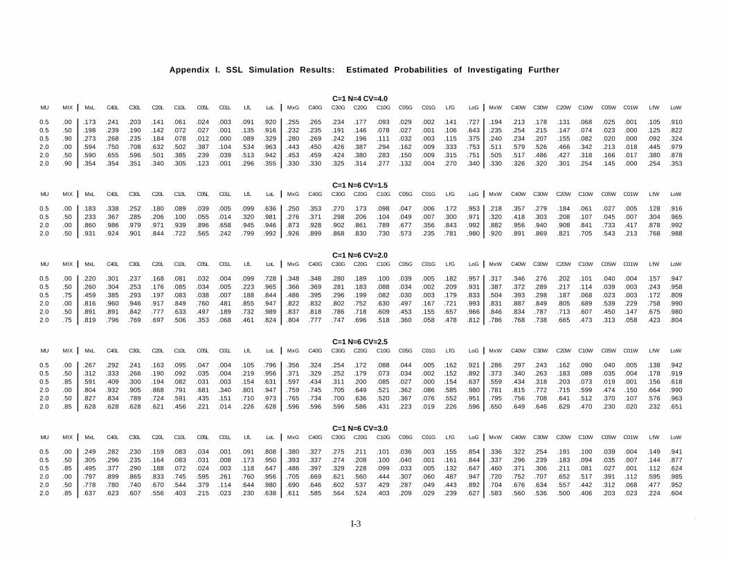
I-33
Appendix I. SSL Simulation Results: Estimated Probabilities of Investigating Further
C=1 N=4 CV=4.0MU MIX MxL C40L C30L C20L C10L C05L C01L LfL LoL MxG C40G C30G C20G C10G C05G C01G LfG LoG MxW C40W C30W C20W C10W C05W C01W LfW LoW
0.5 .00 .173 .241 .203 .141 .061 .024 .003 .091 .920 .255 .265 .234 .177 .093 .029 .002 .141 .727 .194 .213 .178 .131 .068 .025 .001 .105 .9100.5 .50 .198 .239 .190 .142 .072 .027 .001 .135 .916 .232 .235 .191 .146 .078 .027 .001 .106 .643 .235 .254 .215 .147 .074 .023 .000 .125 .8220.5 .90 .273 .268 .235 .184 .078 .012 .000 .089 .329 .280 .269 .242 .196 .111 .032 .003 .115 .375 .240 .234 .207 .155 .082 .020 .000 .092 .3242.0 .00 .594 .750 .708 .632 .502 .387 .104 .534 .963 .443 .450 .426 .387 .294 .162 .009 .333 .753 .511 .579 .526 .466 .342 .213 .018 .445 .9792.0 .50 .590 .655 .596 .501 .385 .239 .039 .513 .942 .453 .459 .424 .380 .283 .150 .009 .315 .751 .505 .517 .486 .427 .318 .166 .017 .380 .8782.0 .90 .354 .354 .351 .340 .305 .123 .001 .296 .355 .330 .330 .325 .314 .277 .132 .004 .270 .340 .330 .326 .320 .301 .254 .145 .000 .254 .353
C=1 N=6 CV=1.5MU MIX MxL C40L C30L C20L C10L C05L C01L LfL LoL MxG C40G C30G C20G C10G C05G C01G LfG LoG MxW C40W C30W C20W C10W C05W C01W LfW LoW
0.5 .00 .183 .338 .252 .180 .089 .039 .005 .099 .636 .250 .353 .270 .173 .098 .047 .006 .172 .953 .218 .357 .279 .184 .061 .027 .005 .128 .9160.5 .50 .233 .367 .285 .206 .100 .055 .014 .320 .981 .276 .371 .298 .206 .104 .049 .007 .300 .971 .320 .418 .303 .208 .107 .045 .007 .304 .9652.0 .00 .860 .986 .979 .971 .939 .896 .658 .945 .946 .873 .928 .902 .861 .789 .677 .356 .843 .992 .882 .956 .940 .908 .841 .733 .417 .878 .9922.0 .50 .931 .924 .901 .844 .722 .565 .242 .799 .992 .926 .899 .868 .830 .730 .573 .235 .781 .980 .920 .891 .869 .821 .705 .543 .213 .768 .988
C=1 N=6 CV=2.0MU MIX MxL C40L C30L C20L C10L C05L C01L LfL LoL MxG C40G C30G C20G C10G C05G C01G LfG LoG MxW C40W C30W C20W C10W C05W C01W LfW LoW
0.5 .00 .220 .301 .237 .168 .081 .032 .004 .099 .728 .348 .348 .280 .189 .100 .039 .005 .182 .957 .317 .346 .276 .202 .101 .040 .004 .157 .9470.5 .50 .260 .304 .253 .176 .085 .034 .005 .223 .965 .366 .369 .281 .183 .088 .034 .002 .209 .931 .387 .372 .289 .217 .114 .039 .003 .243 .9580.5 .75 .459 .385 .293 .197 .083 .038 .007 .188 .844 .486 .395 .296 .199 .082 .030 .003 .179 .833 .504 .393 .298 .187 .068 .023 .003 .172 .8092.0 .00 .816 .960 .946 .917 .849 .760 .481 .855 .947 .822 .832 .802 .752 .630 .497 .167 .721 .993 .831 .887 .849 .805 .689 .539 .229 .758 .9902.0 .50 .891 .891 .842 .777 .633 .497 .189 .732 .989 .837 .818 .786 .718 .609 .453 .155 .657 .966 .846 .834 .787 .713 .607 .450 .147 .675 .9802.0 .75 .819 .796 .769 .697 .506 .353 .068 .461 .824 .804 .777 .747 .696 .518 .360 .058 .478 .812 .786 .768 .738 .665 .473 .313 .058 .423 .804
C=1 N=6 CV=2.5MU MIX MxL C40L C30L C20L C10L C05L C01L LfL LoL MxG C40G C30G C20G C10G C05G C01G LfG LoG MxW C40W C30W C20W C10W C05W C01W LfW LoW
0.5 .00 .267 .292 .241 .163 .095 .047 .004 .105 .796 .356 .324 .254 .172 .088 .044 .005 .162 .921 .286 .297 .243 .162 .090 .040 .005 .138 .9420.5 .50 .312 .333 .266 .190 .092 .035 .004 .219 .956 .371 .329 .252 .179 .073 .034 .002 .152 .892 .373 .340 .263 .183 .089 .035 .004 .178 .9190.5 .85 .591 .409 .300 .194 .082 .031 .003 .154 .631 .597 .434 .311 .200 .085 .027 .000 .154 .637 .559 .434 .318 .203 .073 .019 .001 .156 .6182.0 .00 .804 .932 .905 .868 .791 .681 .340 .801 .947 .759 .745 .705 .649 .521 .362 .086 .585 .980 .781 .815 .772 .715 .599 .474 .150 .664 .9902.0 .50 .827 .834 .789 .724 .591 .435 .151 .710 .973 .765 .734 .700 .636 .520 .367 .076 .552 .951 .795 .756 .708 .641 .512 .370 .107 .576 .9632.0 .85 .628 .628 .628 .621 .456 .221 .014 .226 .628 .596 .596 .596 .586 .431 .223 .019 .226 .596 .650 .649 .646 .629 .470 .230 .020 .232 .651
C=1 N=6 CV=3.0MU MIX MxL C40L C30L C20L C10L C05L C01L LfL LoL MxG C40G C30G C20G C10G C05G C01G LfG LoG MxW C40W C30W C20W C10W C05W C01W LfW LoW
0.5 .00 .249 .282 .230 .159 .083 .034 .001 .091 .808 .380 .327 .275 .211 .101 .036 .003 .155 .854 .336 .322 .254 .191 .100 .039 .004 .149 .9410.5 .50 .305 .296 .235 .164 .083 .031 .008 .173 .950 .393 .337 .274 .208 .100 .040 .001 .161 .844 .337 .296 .239 .183 .094 .035 .007 .144 .8770.5 .85 .495 .377 .290 .188 .072 .024 .003 .118 .647 .486 .397 .329 .228 .099 .033 .005 .132 .647 .460 .371 .306 .211 .081 .027 .001 .112 .6242.0 .00 .797 .899 .865 .833 .745 .595 .261 .760 .956 .705 .669 .621 .560 .444 .307 .060 .487 .947 .720 .752 .707 .652 .517 .391 .112 .595 .9852.0 .50 .778 .780 .740 .670 .544 .379 .114 .644 .980 .690 .646 .602 .537 .429 .287 .049 .443 .892 .704 .676 .634 .557 .442 .312 .068 .477 .9522.0 .85 .637 .623 .607 .556 .403 .215 .023 .230 .638 .611 .585 .564 .524 .403 .209 .029 .239 .627 .583 .560 .536 .500 .406 .203 .023 .224 .604

I-44
Appendix I. SSL Simulation Results: Estimated Probabilities of Investigating Further
C=1 N=6 CV=3.5MU MIX MxL C40L C30L C20L C10L C05L C01L LfL LoL MxG C40G C30G C20G C10G C05G C01G LfG LoG MxW C40W C30W C20W C10W C05W C01W LfW LoW
0.5 .00 .240 .251 .203 .140 .079 .028 .002 .082 .833 .361 .309 .271 .201 .102 .034 .002 .130 .785 .296 .265 .216 .160 .085 .037 .003 .117 .9270.5 .50 .289 .271 .212 .154 .080 .040 .003 .137 .931 .369 .307 .240 .164 .087 .037 .003 .103 .784 .340 .287 .237 .176 .099 .040 .002 .126 .8540.5 .90 .407 .326 .258 .185 .093 .032 .001 .091 .441 .417 .340 .290 .202 .079 .037 .002 .086 .460 .403 .357 .311 .223 .085 .033 .000 .084 .4572.0 .00 .771 .870 .832 .777 .680 .544 .217 .706 .958 .616 .586 .529 .470 .373 .234 .034 .371 .873 .714 .727 .684 .614 .489 .344 .080 .562 .9872.0 .50 .756 .744 .687 .629 .513 .354 .099 .598 .980 .647 .602 .564 .508 .410 .259 .038 .389 .851 .672 .636 .596 .535 .433 .270 .058 .463 .9362.0 .90 .442 .440 .440 .433 .354 .123 .014 .123 .442 .449 .445 .442 .428 .350 .140 .014 .141 .451 .472 .468 .459 .448 .375 .143 .009 .144 .476
C=1 N=6 CV=4.0MU MIX MxL C40L C30L C20L C10L C05L C01L LfL LoL MxG C40G C30G C20G C10G C05G C01G LfG LoG MxW C40W C30W C20W C10W C05W C01W LfW LoW
0.5 .00 .246 .255 .200 .131 .062 .023 .004 .084 .839 .342 .275 .229 .181 .092 .028 .001 .099 .725 .289 .268 .216 .153 .088 .034 .002 .121 .8830.5 .50 .299 .271 .213 .153 .086 .037 .002 .134 .922 .315 .269 .220 .160 .084 .020 .000 .087 .691 .325 .275 .226 .173 .080 .035 .001 .112 .8180.5 .90 .396 .324 .269 .196 .082 .022 .000 .065 .453 .400 .340 .296 .211 .099 .041 .001 .078 .497 .350 .301 .254 .196 .078 .030 .003 .058 .4382.0 .00 .723 .847 .797 .724 .600 .470 .179 .626 .956 .559 .523 .494 .450 .334 .214 .023 .323 .821 .675 .679 .634 .568 .457 .317 .057 .519 .9822.0 .50 .745 .735 .683 .609 .482 .342 .093 .597 .968 .576 .532 .495 .429 .334 .200 .023 .299 .792 .623 .574 .531 .468 .348 .236 .032 .380 .9062.0 .90 .477 .472 .464 .439 .337 .140 .007 .145 .479 .471 .449 .437 .415 .335 .164 .013 .168 .489 .446 .428 .411 .390 .326 .160 .013 .175 .473
C=1 N=9 CV=1.5MU MIX MxL C40L C30L C20L C10L C05L C01L LfL LoL MxG C40G C30G C20G C10G C05G C01G LfG LoG MxW C40W C30W C20W C10W C05W C01W LfW LoW
0.5 .00 .286 .335 .274 .205 .112 .057 .010 .112 .452 .363 .390 .293 .202 .089 .043 .006 .216 .937 .336 .375 .287 .188 .092 .036 .008 .168 .8800.5 .50 .365 .380 .298 .203 .108 .050 .014 .380 .984 .420 .411 .301 .213 .103 .046 .009 .336 .980 .416 .392 .290 .201 .095 .046 .008 .335 .9722.0 .00 .948 .999 .999 .995 .989 .965 .891 .987 .950 .955 .973 .963 .936 .887 .815 .577 .933 .999 .957 .985 .974 .965 .927 .855 .648 .950 .9942.0 .50 .983 .956 .940 .904 .820 .719 .449 .856 .995 .978 .954 .930 .900 .817 .697 .430 .841 .994 .973 .955 .936 .907 .828 .713 .403 .863 .991
C=1 N=9 CV=2.0MU MIX MxL C40L C30L C20L C10L C05L C01L LfL LoL MxG C40G C30G C20G C10G C05G C01G LfG LoG MxW C40W C30W C20W C10W C05W C01W LfW LoW
0.5 .00 .312 .314 .247 .173 .101 .049 .005 .110 .592 .472 .369 .297 .199 .096 .034 .005 .206 .934 .397 .317 .239 .159 .087 .048 .009 .151 .9070.5 .50 .425 .366 .289 .205 .092 .045 .007 .287 .962 .496 .384 .285 .199 .102 .045 .010 .250 .940 .495 .385 .301 .220 .112 .058 .010 .255 .9400.5 .75 .629 .418 .307 .215 .107 .053 .008 .198 .840 .642 .417 .324 .208 .102 .051 .005 .187 .841 .656 .396 .306 .209 .102 .037 .003 .193 .8402.0 .00 .913 .987 .983 .974 .955 .910 .714 .953 .948 .913 .897 .864 .828 .742 .619 .341 .808 .997 .933 .950 .930 .905 .826 .727 .409 .872 .9892.0 .50 .951 .923 .892 .842 .756 .630 .338 .816 .989 .930 .908 .884 .844 .710 .576 .271 .743 .987 .938 .888 .860 .790 .696 .558 .267 .720 .9862.0 .75 .918 .873 .826 .752 .615 .464 .138 .456 .920 .925 .872 .842 .761 .642 .469 .170 .472 .927 .920 .866 .838 .764 .609 .465 .170 .470 .923
C=1 N=9 CV=2.5MU MIX MxL C40L C30L C20L C10L C05L C01L LfL LoL MxG C40G C30G C20G C10G C05G C01G LfG LoG MxW C40W C30W C20W C10W C05W C01W LfW LoW
0.5 .00 .364 .323 .256 .179 .092 .044 .006 .097 .667 .477 .346 .283 .196 .090 .046 .004 .166 .864 .435 .350 .287 .199 .103 .049 .003 .159 .9060.5 .50 .416 .315 .250 .172 .096 .042 .006 .216 .957 .525 .377 .297 .209 .101 .045 .007 .184 .862 .473 .341 .270 .188 .107 .049 .004 .179 .8710.5 .85 .706 .384 .280 .186 .083 .027 .002 .118 .744 .737 .407 .315 .197 .093 .036 .004 .118 .754 .719 .406 .307 .185 .081 .025 .001 .100 .7462.0 .00 .910 .980 .970 .954 .905 .846 .593 .912 .952 .867 .821 .782 .725 .623 .486 .191 .656 .983 .886 .892 .861 .811 .712 .601 .316 .788 .9922.0 .50 .931 .900 .868 .823 .731 .607 .322 .790 .990 .888 .823 .788 .729 .628 .489 .179 .629 .961 .902 .834 .798 .738 .615 .489 .203 .649 .9762.0 .85 .743 .741 .731 .681 .458 .367 .073 .364 .743 .764 .762 .750 .686 .432 .355 .064 .351 .764 .782 .773 .760 .708 .459 .370 .090 .366 .782
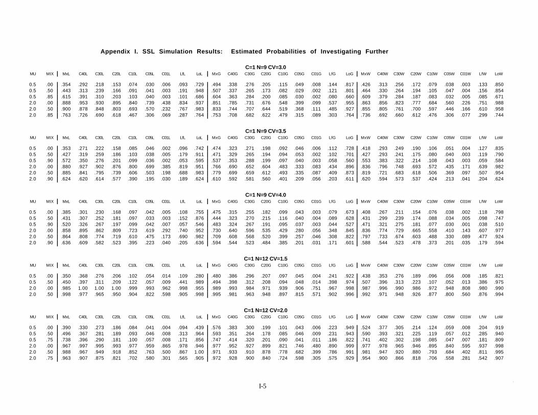
I-55
Appendix I. SSL Simulation Results: Estimated Probabilities of Investigating Further
C=1 N=9 CV=3.0MU MIX MxL C40L C30L C20L C10L C05L C01L LfL LoL MxG C40G C30G C20G C10G C05G C01G LfG LoG MxW C40W C30W C20W C10W C05W C01W LfW LoW
0.5 .00 .354 .292 .218 .153 .074 .030 .006 .093 .729 .494 .338 .276 .205 .115 .049 .008 .144 .817 .426 .313 .256 .172 .079 .038 .003 .133 .8500.5 .50 .443 .313 .239 .166 .091 .041 .003 .191 .948 .507 .337 .265 .173 .082 .029 .002 .121 .801 .464 .330 .264 .194 .105 .047 .004 .156 .8540.5 .85 .615 .391 .310 .203 .103 .040 .003 .101 .686 .604 .363 .284 .200 .085 .030 .002 .080 .660 .609 .379 .284 .187 .083 .032 .005 .085 .6712.0 .00 .888 .953 .930 .895 .840 .739 .438 .834 .937 .851 .785 .731 .676 .548 .399 .099 .537 .955 .863 .856 .823 .777 .684 .560 .226 .751 .9882.0 .50 .900 .878 .848 .803 .693 .570 .232 .767 .983 .833 .744 .707 .644 .519 .368 .111 .485 .927 .855 .805 .761 .700 .597 .446 .166 .610 .9582.0 .85 .763 .726 .690 .618 .467 .306 .069 .287 .764 .753 .708 .682 .622 .479 .315 .089 .303 .764 .736 .692 .660 .612 .476 .306 .077 .299 .744
C=1 N=9 CV=3.5MU MIX MxL C40L C30L C20L C10L C05L C01L LfL LoL MxG C40G C30G C20G C10G C05G C01G LfG LoG MxW C40W C30W C20W C10W C05W C01W LfW LoW
0.5 .00 .353 .271 .222 .158 .085 .046 .002 .096 .742 .474 .323 .271 .198 .092 .046 .006 .112 .728 .418 .293 .249 .190 .106 .051 .004 .127 .8350.5 .50 .427 .319 .259 .186 .103 .038 .005 .179 .911 .471 .329 .265 .194 .094 .053 .002 .102 .701 .427 .293 .241 .175 .080 .040 .003 .119 .7900.5 .90 .572 .350 .276 .201 .099 .036 .002 .053 .595 .537 .353 .288 .199 .097 .040 .003 .058 .560 .553 .383 .322 .214 .108 .043 .003 .059 .5842.0 .00 .880 .927 .902 .876 .800 .699 .385 .819 .951 .766 .690 .652 .604 .483 .333 .083 .434 .896 .836 .796 .748 .693 .572 .435 .171 .639 .9822.0 .50 .885 .841 .795 .739 .606 .503 .198 .688 .983 .779 .699 .659 .612 .493 .335 .087 .409 .873 .819 .721 .683 .618 .506 .369 .097 .507 .9542.0 .90 .624 .620 .614 .577 .390 .195 .030 .189 .624 .610 .592 .581 .560 .401 .209 .056 .203 .611 .620 .594 .573 .537 .424 .213 .041 .204 .624
C=1 N=9 CV=4.0MU MIX MxL C40L C30L C20L C10L C05L C01L LfL LoL MxG C40G C30G C20G C10G C05G C01G LfG LoG MxW C40W C30W C20W C10W C05W C01W LfW LoW
0.5 .00 .385 .301 .230 .168 .097 .042 .005 .108 .755 .475 .315 .255 .182 .099 .043 .003 .079 .673 .408 .267 .211 .154 .076 .038 .002 .118 .7980.5 .50 .431 .307 .252 .181 .097 .033 .003 .152 .876 .444 .323 .270 .215 .116 .040 .004 .089 .628 .431 .299 .239 .174 .088 .034 .005 .098 .7470.5 .90 .520 .326 .267 .197 .099 .042 .007 .057 .546 .483 .324 .267 .191 .095 .037 .003 .044 .527 .471 .321 .275 .181 .077 .030 .001 .038 .5102.0 .00 .858 .895 .862 .809 .723 .619 .292 .740 .952 .730 .640 .596 .535 .429 .280 .056 .348 .845 .836 .774 .729 .665 .558 .410 .143 .607 .9772.0 .50 .864 .808 .774 .719 .610 .475 .173 .690 .982 .709 .608 .568 .520 .399 .257 .046 .308 .822 .797 .733 .674 .603 .488 .330 .089 .477 .9242.0 .90 .636 .609 .582 .523 .395 .223 .040 .205 .636 .594 .544 .523 .484 .385 .201 .031 .171 .601 .588 .544 .523 .478 .373 .201 .035 .179 .594
C=1 N=12 CV=1.5MU MIX MxL C40L C30L C20L C10L C05L C01L LfL LoL MxG C40G C30G C20G C10G C05G C01G LfG LoG MxW C40W C30W C20W C10W C05W C01W LfW LoW
0.5 .00 .350 .368 .276 .206 .102 .054 .014 .109 .280 .480 .386 .296 .207 .097 .045 .004 .241 .922 .438 .353 .276 .189 .096 .056 .008 .185 .8210.5 .50 .450 .397 .311 .209 .122 .057 .009 .441 .989 .494 .398 .312 .208 .094 .048 .014 .398 .974 .507 .396 .313 .223 .107 .052 .013 .386 .9752.0 .00 .985 1.00 1.00 1.00 .999 .993 .962 .998 .955 .989 .993 .984 .971 .939 .906 .751 .967 .998 .987 .996 .990 .986 .972 .948 .808 .980 .9902.0 .50 .998 .977 .965 .950 .904 .822 .598 .905 .998 .995 .981 .963 .948 .897 .815 .571 .902 .996 .992 .971 .948 .926 .877 .800 .560 .876 .994
C=1 N=12 CV=2.0MU MIX MxL C40L C30L C20L C10L C05L C01L LfL LoL MxG C40G C30G C20G C10G C05G C01G LfG LoG MxW C40W C30W C20W C10W C05W C01W LfW LoW
0.5 .00 .390 .330 .273 .186 .084 .041 .004 .094 .439 .576 .383 .300 .199 .101 .043 .006 .223 .949 .524 .377 .305 .214 .124 .059 .008 .204 .9190.5 .50 .496 .367 .281 .189 .093 .046 .008 .313 .964 .593 .351 .264 .178 .085 .046 .009 .231 .943 .590 .393 .321 .225 .119 .057 .012 .285 .9400.5 .75 .738 .396 .290 .181 .100 .057 .008 .171 .856 .747 .414 .320 .201 .090 .041 .011 .186 .822 .741 .402 .302 .198 .085 .047 .007 .181 .8092.0 .00 .967 .997 .995 .993 .977 .959 .865 .978 .946 .977 .952 .927 .899 .821 .746 .480 .890 .999 .977 .978 .965 .946 .895 .840 .595 .937 .9982.0 .50 .988 .967 .949 .918 .852 .763 .500 .867 1.00 .971 .933 .910 .878 .778 .682 .399 .786 .991 .981 .947 .920 .880 .793 .684 .402 .811 .9952.0 .75 .963 .907 .875 .821 .702 .580 .301 .565 .905 .972 .928 .900 .840 .724 .598 .305 .575 .929 .954 .900 .866 .818 .706 .558 .281 .542 .907

I-66
Appendix I. SSL Simulation Results: Estimated Probabilities of Investigating Further
C=1 N=12 CV=2.5MU MIX MxL C40L C30L C20L C10L C05L C01L LfL LoL MxG C40G C30G C20G C10G C05G C01G LfG LoG MxW C40W C30W C20W C10W C05W C01W LfW LoW
0.5 .00 .435 .296 .223 .159 .084 .038 .005 .089 .520 .627 .375 .293 .201 .092 .040 .006 .176 .902 .530 .340 .273 .190 .088 .038 .005 .164 .8980.5 .50 .492 .305 .234 .175 .083 .041 .006 .227 .942 .623 .384 .287 .195 .087 .042 .007 .159 .878 .614 .377 .285 .197 .093 .045 .005 .187 .9100.5 .85 .833 .413 .312 .194 .104 .036 .003 .092 .596 .802 .411 .308 .216 .097 .046 .009 .091 .558 .814 .387 .290 .195 .086 .037 .003 .086 .5392.0 .00 .968 .991 .984 .982 .959 .921 .720 .963 .956 .939 .879 .852 .803 .703 .583 .289 .742 .991 .965 .948 .919 .877 .816 .709 .406 .873 .9962.0 .50 .969 .940 .914 .877 .799 .686 .395 .844 .995 .951 .882 .850 .795 .691 .577 .257 .684 .976 .954 .894 .860 .824 .736 .624 .307 .731 .9832.0 .85 .859 .844 .812 .720 .544 .406 .116 .250 .842 .851 .835 .807 .715 .568 .455 .120 .264 .830 .856 .829 .798 .730 .549 .438 .134 .255 .822
C=1 N=12 CV=3.0MU MIX MxL C40L C30L C20L C10L C05L C01L LfL LoL MxG C40G C30G C20G C10G C05G C01G LfG LoG MxW C40W C30W C20W C10W C05W C01W LfW LoW
0.5 .00 .429 .311 .239 .162 .079 .042 .005 .092 .612 .600 .365 .283 .197 .099 .043 .004 .119 .806 .547 .337 .258 .190 .090 .047 .006 .145 .8700.5 .50 .510 .322 .253 .187 .109 .043 .005 .217 .930 .610 .365 .300 .211 .114 .059 .005 .148 .778 .565 .355 .269 .192 .093 .048 .006 .149 .8420.5 .85 .728 .381 .290 .205 .117 .056 .012 .088 .593 .707 .358 .283 .198 .107 .052 .004 .089 .540 .713 .404 .315 .225 .118 .053 .004 .090 .5912.0 .00 .933 .972 .959 .932 .900 .843 .605 .909 .932 .925 .821 .784 .724 .608 .492 .183 .587 .964 .933 .901 .873 .832 .754 .634 .310 .808 .9922.0 .50 .955 .917 .883 .843 .748 .634 .318 .797 .991 .909 .826 .786 .719 .599 .458 .167 .520 .943 .912 .852 .814 .752 .634 .510 .227 .637 .9722.0 .85 .844 .769 .718 .631 .511 .364 .124 .252 .760 .852 .786 .745 .680 .535 .378 .130 .267 .784 .820 .755 .716 .657 .529 .380 .119 .250 .762
C=1 N=12 CV=3.5MU MIX MxL C40L C30L C20L C10L C05L C01L LfL LoL MxG C40G C30G C20G C10G C05G C01G LfG LoG MxW C40W C30W C20W C10W C05W C01W LfW LoW
0.5 .00 .437 .307 .237 .174 .095 .044 .005 .111 .660 .608 .360 .294 .214 .108 .042 .005 .109 .735 .505 .316 .260 .194 .110 .046 .004 .139 .8410.5 .50 .508 .305 .238 .174 .094 .040 .003 .173 .908 .589 .325 .259 .182 .082 .046 .004 .088 .708 .541 .301 .247 .179 .093 .039 .006 .110 .7880.5 .90 .680 .377 .299 .196 .085 .037 .001 .033 .409 .666 .388 .304 .204 .100 .050 .004 .055 .424 .632 .386 .316 .235 .121 .047 .005 .049 .4342.0 .00 .940 .957 .934 .912 .857 .777 .522 .863 .952 .870 .760 .712 .648 .529 .394 .134 .445 .929 .918 .870 .838 .792 .677 .563 .238 .747 .9912.0 .50 .945 .900 .863 .809 .715 .596 .284 .765 .989 .866 .749 .690 .627 .506 .359 .108 .398 .889 .886 .783 .737 .668 .572 .438 .176 .561 .9632.0 .90 .723 .710 .684 .628 .420 .295 .083 .147 .703 .709 .685 .656 .598 .439 .283 .092 .158 .681 .708 .672 .654 .605 .445 .288 .091 .166 .670
C=1 N=12 CV=4.0MU MIX MxL C40L C30L C20L C10L C05L C01L LfL LoL MxG C40G C30G C20G C10G C05G C01G LfG LoG MxW C40W C30W C20W C10W C05W C01W LfW LoW
0.5 .00 .470 .290 .226 .169 .090 .043 .005 .103 .699 .559 .317 .261 .197 .107 .049 .005 .081 .640 .525 .328 .273 .201 .099 .047 .004 .116 .8480.5 .50 .495 .313 .263 .173 .098 .043 .002 .152 .904 .563 .319 .260 .182 .108 .043 .004 .080 .632 .559 .340 .274 .197 .097 .045 .006 .107 .7850.5 .90 .638 .351 .289 .193 .094 .051 .007 .052 .425 .605 .365 .304 .204 .095 .043 .004 .040 .442 .585 .343 .282 .196 .093 .049 .002 .046 .4122.0 .00 .942 .950 .926 .899 .824 .740 .471 .838 .955 .830 .705 .667 .605 .490 .347 .093 .374 .861 .883 .803 .760 .710 .618 .497 .181 .668 .9832.0 .50 .930 .849 .819 .769 .673 .561 .227 .736 .985 .817 .689 .640 .586 .481 .317 .087 .325 .830 .880 .774 .735 .678 .555 .415 .136 .508 .9452.0 .90 .713 .672 .640 .575 .425 .286 .074 .151 .666 .710 .652 .621 .569 .437 .257 .051 .139 .654 .706 .647 .611 .568 .443 .252 .061 .148 .643
C=1 N=16 CV=1.5MU MIX MxL C40L C30L C20L C10L C05L C01L LfL LoL MxG C40G C30G C20G C10G C05G C01G LfG LoG MxW C40W C30W C20W C10W C05W C01W LfW LoW
0.5 .00 .438 .354 .279 .202 .102 .053 .007 .092 .161 .565 .393 .307 .216 .100 .058 .012 .293 .900 .542 .371 .287 .196 .111 .054 .010 .223 .8010.5 .50 .535 .387 .303 .205 .110 .062 .014 .482 .986 .586 .411 .291 .200 .111 .052 .004 .459 .976 .595 .400 .292 .204 .103 .062 .007 .447 .9782.0 .00 .996 1.00 1.00 1.00 1.00 1.00 .997 1.00 .957 .994 .995 .992 .989 .975 .956 .872 .989 .999 .993 .997 .996 .990 .983 .973 .924 .988 .9952.0 .50 1.00 .990 .982 .973 .950 .910 .761 .945 1.00 .999 .988 .982 .959 .925 .875 .714 .932 .998 .998 .987 .976 .962 .928 .885 .734 .922 .999
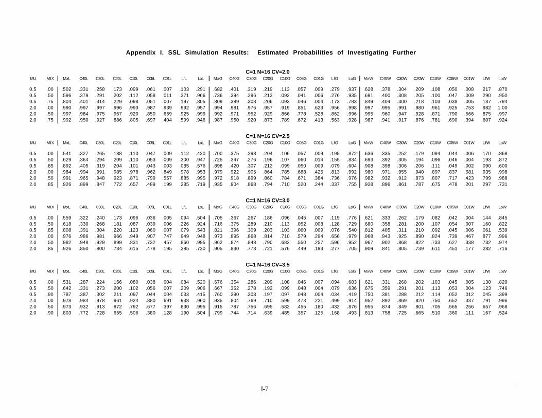
I-77
Appendix I. SSL Simulation Results: Estimated Probabilities of Investigating Further
C=1 N=16 CV=2.0MU MIX MxL C40L C30L C20L C10L C05L C01L LfL LoL MxG C40G C30G C20G C10G C05G C01G LfG LoG MxW C40W C30W C20W C10W C05W C01W LfW LoW
0.5 .00 .502 .331 .258 .173 .099 .061 .007 .103 .291 .682 .401 .319 .219 .113 .057 .009 .279 .937 .628 .378 .304 .209 .108 .050 .008 .217 .8700.5 .50 .596 .379 .291 .202 .112 .058 .011 .371 .966 .736 .394 .296 .213 .092 .041 .006 .276 .935 .691 .400 .308 .205 .100 .047 .009 .290 .9500.5 .75 .804 .401 .314 .229 .098 .051 .007 .197 .805 .809 .389 .308 .206 .093 .046 .004 .173 .783 .849 .404 .300 .218 .103 .038 .005 .187 .7942.0 .00 .990 .997 .997 .996 .993 .987 .939 .992 .957 .994 .981 .976 .957 .919 .851 .623 .956 .998 .997 .995 .991 .980 .961 .925 .753 .982 1.002.0 .50 .997 .984 .975 .957 .920 .850 .659 .925 .999 .992 .971 .952 .929 .866 .778 .528 .862 .996 .995 .960 .947 .928 .871 .790 .566 .875 .9972.0 .75 .992 .950 .927 .886 .805 .697 .404 .599 .946 .987 .950 .920 .873 .789 .672 .413 .563 .928 .987 .941 .917 .876 .781 .690 .394 .607 .924
C=1 N=16 CV=2.5MU MIX MxL C40L C30L C20L C10L C05L C01L LfL LoL MxG C40G C30G C20G C10G C05G C01G LfG LoG MxW C40W C30W C20W C10W C05W C01W LfW LoW
0.5 .00 .541 .327 .265 .188 .110 .047 .009 .112 .420 .700 .375 .298 .204 .106 .057 .009 .195 .872 .636 .335 .252 .179 .094 .044 .006 .170 .8680.5 .50 .629 .364 .294 .209 .110 .053 .009 .300 .947 .725 .347 .276 .196 .107 .060 .014 .155 .834 .693 .392 .305 .194 .096 .046 .004 .193 .8720.5 .85 .892 .405 .319 .204 .101 .043 .003 .085 .576 .898 .420 .307 .212 .099 .050 .009 .079 .604 .908 .398 .306 .206 .111 .049 .002 .090 .6002.0 .00 .984 .994 .991 .985 .978 .962 .849 .978 .953 .979 .922 .905 .864 .785 .688 .425 .813 .992 .980 .971 .955 .940 .897 .837 .581 .935 .9982.0 .50 .991 .965 .948 .923 .871 .799 .557 .885 .995 .972 .918 .899 .860 .784 .671 .384 .736 .976 .982 .932 .912 .873 .807 .717 .423 .799 .9882.0 .85 .926 .899 .847 .772 .657 .489 .199 .285 .719 .935 .904 .868 .794 .710 .520 .244 .337 .755 .928 .896 .861 .787 .675 .478 .201 .297 .731
C=1 N=16 CV=3.0MU MIX MxL C40L C30L C20L C10L C05L C01L LfL LoL MxG C40G C30G C20G C10G C05G C01G LfG LoG MxW C40W C30W C20W C10W C05W C01W LfW LoW
0.5 .00 .559 .322 .240 .173 .096 .036 .005 .094 .504 .705 .367 .267 .186 .096 .045 .007 .119 .776 .621 .333 .262 .179 .082 .042 .004 .144 .8450.5 .50 .618 .330 .268 .181 .087 .039 .006 .226 .924 .716 .375 .289 .210 .113 .052 .008 .128 .729 .680 .358 .281 .200 .107 .054 .007 .160 .8220.5 .85 .808 .391 .304 .220 .123 .060 .007 .079 .543 .821 .396 .309 .203 .103 .060 .009 .076 .540 .812 .405 .311 .210 .092 .045 .006 .061 .5392.0 .00 .976 .986 .981 .966 .949 .907 .747 .949 .948 .973 .895 .868 .814 .710 .579 .294 .656 .979 .968 .943 .925 .890 .824 .739 .467 .877 .9962.0 .50 .982 .948 .929 .899 .831 .732 .457 .860 .995 .962 .874 .848 .790 .682 .550 .257 .596 .952 .967 .902 .868 .822 .733 .627 .338 .732 .9742.0 .85 .926 .850 .800 .734 .615 .478 .195 .285 .720 .905 .830 .773 .721 .576 .449 .193 .277 .705 .909 .841 .805 .739 .611 .451 .177 .282 .716
C=1 N=16 CV=3.5MU MIX MxL C40L C30L C20L C10L C05L C01L LfL LoL MxG C40G C30G C20G C10G C05G C01G LfG LoG MxW C40W C30W C20W C10W C05W C01W LfW LoW
0.5 .00 .531 .287 .224 .156 .080 .038 .004 .084 .520 .676 .354 .286 .209 .108 .046 .007 .094 .683 .621 .331 .268 .202 .103 .045 .005 .130 .8200.5 .50 .642 .331 .273 .200 .102 .056 .007 .209 .906 .667 .352 .278 .192 .099 .048 .004 .079 .636 .675 .359 .291 .201 .113 .053 .004 .123 .7460.5 .90 .787 .387 .302 .211 .097 .044 .004 .033 .415 .760 .390 .303 .197 .097 .048 .004 .034 .419 .750 .381 .288 .212 .114 .052 .012 .045 .3992.0 .00 .978 .984 .978 .961 .924 .880 .691 .938 .960 .935 .804 .769 .710 .599 .473 .221 .499 .914 .952 .892 .869 .820 .750 .652 .337 .791 .9962.0 .50 .973 .932 .913 .872 .792 .677 .397 .830 .995 .915 .787 .756 .695 .582 .455 .180 .432 .876 .955 .874 .849 .801 .705 .565 .256 .657 .9682.0 .90 .803 .772 .728 .655 .506 .380 .128 .190 .504 .799 .744 .714 .639 .485 .357 .125 .168 .493 .813 .758 .725 .665 .510 .360 .111 .167 .524
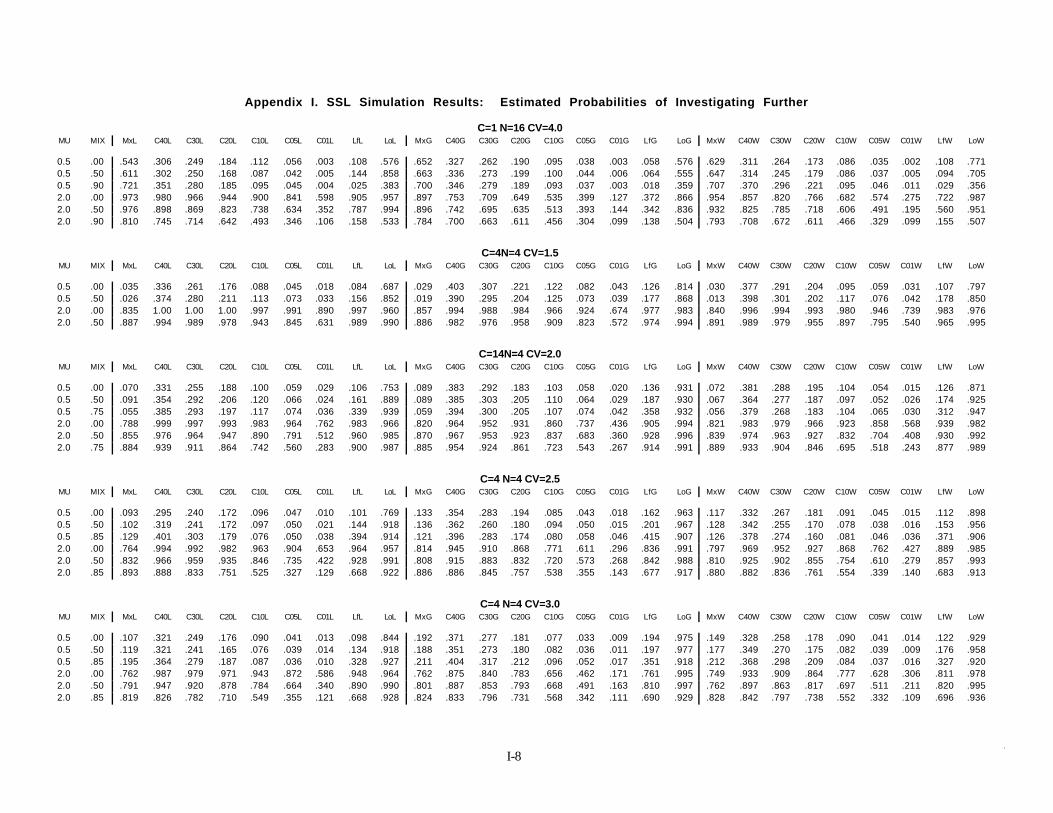
I-88
Appendix I. SSL Simulation Results: Estimated Probabilities of Investigating Further
C=1 N=16 CV=4.0MU MIX MxL C40L C30L C20L C10L C05L C01L LfL LoL MxG C40G C30G C20G C10G C05G C01G LfG LoG MxW C40W C30W C20W C10W C05W C01W LfW LoW
0.5 .00 .543 .306 .249 .184 .112 .056 .003 .108 .576 .652 .327 .262 .190 .095 .038 .003 .058 .576 .629 .311 .264 .173 .086 .035 .002 .108 .7710.5 .50 .611 .302 .250 .168 .087 .042 .005 .144 .858 .663 .336 .273 .199 .100 .044 .006 .064 .555 .647 .314 .245 .179 .086 .037 .005 .094 .7050.5 .90 .721 .351 .280 .185 .095 .045 .004 .025 .383 .700 .346 .279 .189 .093 .037 .003 .018 .359 .707 .370 .296 .221 .095 .046 .011 .029 .3562.0 .00 .973 .980 .966 .944 .900 .841 .598 .905 .957 .897 .753 .709 .649 .535 .399 .127 .372 .866 .954 .857 .820 .766 .682 .574 .275 .722 .9872.0 .50 .976 .898 .869 .823 .738 .634 .352 .787 .994 .896 .742 .695 .635 .513 .393 .144 .342 .836 .932 .825 .785 .718 .606 .491 .195 .560 .9512.0 .90 .810 .745 .714 .642 .493 .346 .106 .158 .533 .784 .700 .663 .611 .456 .304 .099 .138 .504 .793 .708 .672 .611 .466 .329 .099 .155 .507
C=4N=4 CV=1.5MU MIX MxL C40L C30L C20L C10L C05L C01L LfL LoL MxG C40G C30G C20G C10G C05G C01G LfG LoG MxW C40W C30W C20W C10W C05W C01W LfW LoW
0.5 .00 .035 .336 .261 .176 .088 .045 .018 .084 .687 .029 .403 .307 .221 .122 .082 .043 .126 .814 .030 .377 .291 .204 .095 .059 .031 .107 .7970.5 .50 .026 .374 .280 .211 .113 .073 .033 .156 .852 .019 .390 .295 .204 .125 .073 .039 .177 .868 .013 .398 .301 .202 .117 .076 .042 .178 .8502.0 .00 .835 1.00 1.00 1.00 .997 .991 .890 .997 .960 .857 .994 .988 .984 .966 .924 .674 .977 .983 .840 .996 .994 .993 .980 .946 .739 .983 .9762.0 .50 .887 .994 .989 .978 .943 .845 .631 .989 .990 .886 .982 .976 .958 .909 .823 .572 .974 .994 .891 .989 .979 .955 .897 .795 .540 .965 .995
C=14N=4 CV=2.0MU MIX MxL C40L C30L C20L C10L C05L C01L LfL LoL MxG C40G C30G C20G C10G C05G C01G LfG LoG MxW C40W C30W C20W C10W C05W C01W LfW LoW
0.5 .00 .070 .331 .255 .188 .100 .059 .029 .106 .753 .089 .383 .292 .183 .103 .058 .020 .136 .931 .072 .381 .288 .195 .104 .054 .015 .126 .8710.5 .50 .091 .354 .292 .206 .120 .066 .024 .161 .889 .089 .385 .303 .205 .110 .064 .029 .187 .930 .067 .364 .277 .187 .097 .052 .026 .174 .9250.5 .75 .055 .385 .293 .197 .117 .074 .036 .339 .939 .059 .394 .300 .205 .107 .074 .042 .358 .932 .056 .379 .268 .183 .104 .065 .030 .312 .9472.0 .00 .788 .999 .997 .993 .983 .964 .762 .983 .966 .820 .964 .952 .931 .860 .737 .436 .905 .994 .821 .983 .979 .966 .923 .858 .568 .939 .9822.0 .50 .855 .976 .964 .947 .890 .791 .512 .960 .985 .870 .967 .953 .923 .837 .683 .360 .928 .996 .839 .974 .963 .927 .832 .704 .408 .930 .9922.0 .75 .884 .939 .911 .864 .742 .560 .283 .900 .987 .885 .954 .924 .861 .723 .543 .267 .914 .991 .889 .933 .904 .846 .695 .518 .243 .877 .989
C=4 N=4 CV=2.5MU MIX MxL C40L C30L C20L C10L C05L C01L LfL LoL MxG C40G C30G C20G C10G C05G C01G LfG LoG MxW C40W C30W C20W C10W C05W C01W LfW LoW
0.5 .00 .093 .295 .240 .172 .096 .047 .010 .101 .769 .133 .354 .283 .194 .085 .043 .018 .162 .963 .117 .332 .267 .181 .091 .045 .015 .112 .8980.5 .50 .102 .319 .241 .172 .097 .050 .021 .144 .918 .136 .362 .260 .180 .094 .050 .015 .201 .967 .128 .342 .255 .170 .078 .038 .016 .153 .9560.5 .85 .129 .401 .303 .179 .076 .050 .038 .394 .914 .121 .396 .283 .174 .080 .058 .046 .415 .907 .126 .378 .274 .160 .081 .046 .036 .371 .9062.0 .00 .764 .994 .992 .982 .963 .904 .653 .964 .957 .814 .945 .910 .868 .771 .611 .296 .836 .991 .797 .969 .952 .927 .868 .762 .427 .889 .9852.0 .50 .832 .966 .959 .935 .846 .735 .422 .928 .991 .808 .915 .883 .832 .720 .573 .268 .842 .988 .810 .925 .902 .855 .754 .610 .279 .857 .9932.0 .85 .893 .888 .833 .751 .525 .327 .129 .668 .922 .886 .886 .845 .757 .538 .355 .143 .677 .917 .880 .882 .836 .761 .554 .339 .140 .683 .913
C=4 N=4 CV=3.0MU MIX MxL C40L C30L C20L C10L C05L C01L LfL LoL MxG C40G C30G C20G C10G C05G C01G LfG LoG MxW C40W C30W C20W C10W C05W C01W LfW LoW
0.5 .00 .107 .321 .249 .176 .090 .041 .013 .098 .844 .192 .371 .277 .181 .077 .033 .009 .194 .975 .149 .328 .258 .178 .090 .041 .014 .122 .9290.5 .50 .119 .321 .241 .165 .076 .039 .014 .134 .918 .188 .351 .273 .180 .082 .036 .011 .197 .977 .177 .349 .270 .175 .082 .039 .009 .176 .9580.5 .85 .195 .364 .279 .187 .087 .036 .010 .328 .927 .211 .404 .317 .212 .096 .052 .017 .351 .918 .212 .368 .298 .209 .084 .037 .016 .327 .9202.0 .00 .762 .987 .979 .971 .943 .872 .586 .948 .964 .762 .875 .840 .783 .656 .462 .171 .761 .995 .749 .933 .909 .864 .777 .628 .306 .811 .9782.0 .50 .791 .947 .920 .878 .784 .664 .340 .890 .990 .801 .887 .853 .793 .668 .491 .163 .810 .997 .762 .897 .863 .817 .697 .511 .211 .820 .9952.0 .85 .819 .826 .782 .710 .549 .355 .121 .668 .928 .824 .833 .796 .731 .568 .342 .111 .690 .929 .828 .842 .797 .738 .552 .332 .109 .696 .936

I-99
Appendix I. SSL Simulation Results: Estimated Probabilities of Investigating Further
C=4 N=4 CV=3.5MU MIX MxL C40L C30L C20L C10L C05L C01L LfL LoL MxG C40G C30G C20G C10G C05G C01G LfG LoG MxW C40W C30W C20W C10W C05W C01W LfW LoW
0.5 .00 .116 .279 .220 .154 .082 .038 .008 .091 .834 .242 .376 .295 .196 .090 .033 .008 .219 .975 .171 .303 .246 .174 .082 .038 .008 .126 .9320.5 .50 .140 .308 .239 .166 .083 .042 .009 .134 .934 .236 .362 .287 .201 .097 .042 .009 .239 .978 .183 .327 .255 .168 .083 .038 .010 .165 .9800.5 .90 .260 .371 .289 .188 .083 .038 .013 .315 .806 .291 .403 .304 .189 .080 .032 .010 .330 .822 .284 .376 .278 .173 .078 .029 .009 .295 .8032.0 .00 .749 .979 .974 .952 .902 .829 .517 .909 .970 .712 .808 .763 .697 .573 .406 .125 .712 .992 .728 .903 .871 .834 .715 .568 .241 .770 .9832.0 .50 .753 .928 .901 .857 .756 .629 .306 .853 .988 .736 .806 .769 .714 .582 .371 .125 .720 .994 .750 .871 .828 .770 .642 .488 .193 .757 .9962.0 .90 .784 .780 .744 .675 .510 .278 .074 .574 .826 .786 .782 .732 .671 .495 .255 .067 .569 .826 .773 .764 .730 .665 .488 .251 .050 .574 .824
C=4 N=4 CV=4.0MU MIX MxL C40L C30L C20L C10L C05L C01L LfL LoL MxG C40G C30G C20G C10G C05G C01G LfG LoG MxW C40W C30W C20W C10W C05W C01W LfW LoW
0.5 .00 .125 .263 .210 .148 .079 .038 .007 .090 .849 .277 .358 .291 .202 .096 .040 .007 .226 .964 .174 .302 .236 .173 .087 .037 .009 .131 .9380.5 .50 .162 .303 .240 .173 .085 .039 .008 .146 .945 .251 .339 .261 .182 .082 .034 .007 .205 .957 .233 .336 .286 .198 .108 .043 .010 .192 .9690.5 .90 .297 .371 .293 .196 .070 .024 .007 .276 .823 .307 .376 .288 .198 .076 .033 .009 .266 .800 .307 .382 .297 .182 .066 .029 .009 .265 .8132.0 .00 .711 .966 .953 .929 .856 .768 .441 .865 .959 .680 .751 .714 .655 .512 .330 .086 .664 .994 .709 .859 .832 .780 .671 .519 .171 .729 .9842.0 .50 .737 .907 .871 .825 .728 .559 .238 .814 .990 .699 .753 .704 .640 .519 .319 .075 .657 .981 .690 .798 .765 .699 .573 .410 .134 .713 .9922.0 .90 .721 .718 .684 .626 .442 .244 .056 .544 .814 .716 .720 .686 .627 .458 .236 .047 .543 .833 .695 .696 .660 .603 .445 .239 .054 .539 .800
C=4 N=6 CV=1.5MU MIX MxL C40L C30L C20L C10L C05L C01L LfL LoL MxG C40G C30G C20G C10G C05G C01G LfG LoG MxW C40W C30W C20W C10W C05W C01W LfW LoW
0.5 .00 .048 .336 .262 .185 .092 .039 .013 .087 .315 .042 .390 .305 .203 .103 .056 .022 .122 .604 .043 .391 .293 .196 .088 .045 .018 .098 .5720.5 .50 .047 .401 .309 .209 .120 .060 .028 .205 .685 .024 .383 .308 .214 .106 .062 .030 .210 .741 .027 .407 .306 .212 .111 .064 .021 .213 .7692.0 .00 .928 1.00 1.00 1.00 1.00 .999 .993 1.00 .965 .961 1.00 1.00 1.00 .997 .994 .918 .999 .986 .940 1.00 1.00 1.00 1.00 .993 .931 .998 .9812.0 .50 .964 .999 .998 .995 .981 .947 .803 .997 .992 .966 .998 .996 .988 .973 .941 .783 .996 .998 .962 .999 .998 .995 .985 .951 .781 .999 .995
C=4 N=6 CV=2.0MU MIX MxL C40L C30L C20L C10L C05L C01L LfL LoL MxG C40G C30G C20G C10G C05G C01G LfG LoG MxW C40W C30W C20W C10W C05W C01W LfW LoW
0.5 .00 .091 .368 .288 .193 .105 .058 .020 .111 .481 .106 .369 .285 .187 .089 .044 .013 .129 .843 .113 .364 .278 .182 .091 .046 .008 .111 .7380.5 .50 .089 .378 .293 .205 .108 .049 .011 .174 .805 .112 .382 .293 .206 .118 .073 .019 .231 .900 .122 .390 .300 .198 .100 .053 .018 .214 .8990.5 .75 .075 .390 .298 .209 .114 .066 .026 .457 .944 .090 .398 .311 .207 .101 .054 .022 .434 .951 .088 .409 .303 .194 .100 .051 .022 .446 .9602.0 .00 .906 1.00 1.00 1.00 .998 .996 .966 .999 .963 .930 .991 .984 .978 .960 .913 .693 .966 .992 .923 .997 .996 .991 .977 .960 .810 .978 .9782.0 .50 .937 .994 .992 .982 .965 .916 .715 .995 .992 .943 .985 .979 .966 .916 .852 .594 .972 .997 .947 .996 .987 .977 .946 .884 .642 .984 .9962.0 .75 .952 .967 .951 .924 .848 .753 .429 .941 .998 .960 .973 .960 .942 .879 .770 .431 .953 .999 .964 .971 .960 .931 .851 .741 .408 .941 1.00
C=4 N=6 CV=2.5MU MIX MxL C40L C30L C20L C10L C05L C01L LfL LoL MxG C40G C30G C20G C10G C05G C01G LfG LoG MxW C40W C30W C20W C10W C05W C01W LfW LoW
0.5 .00 .134 .347 .274 .187 .109 .062 .009 .119 .554 .200 .385 .292 .206 .099 .040 .010 .183 .906 .158 .336 .268 .188 .096 .053 .006 .133 .8050.5 .50 .186 .383 .293 .210 .097 .048 .010 .176 .844 .212 .385 .294 .195 .095 .042 .008 .234 .958 .198 .376 .299 .203 .093 .049 .007 .212 .9380.5 .85 .175 .363 .264 .163 .087 .050 .023 .406 .970 .178 .389 .292 .204 .091 .043 .014 .435 .975 .196 .418 .308 .203 .107 .048 .019 .445 .9682.0 .00 .889 .997 .997 .997 .990 .983 .891 .993 .968 .907 .975 .957 .929 .885 .805 .514 .923 .994 .893 .993 .987 .976 .941 .895 .658 .952 .9812.0 .50 .911 .989 .983 .963 .936 .887 .642 .977 .997 .917 .963 .950 .923 .860 .771 .455 .941 .997 .926 .976 .967 .948 .898 .810 .531 .956 .9992.0 .85 .980 .941 .913 .854 .710 .534 .204 .837 .984 .953 .913 .885 .834 .685 .517 .186 .818 .972 .974 .944 .914 .869 .744 .565 .204 .854 .983

I-101 0
Appendix I. SSL Simulation Results: Estimated Probabilities of Investigating Further.
C=4 N=6 CV=3.0MU MIX MxL C40L C30L C20L C10L C05L C01L LfL LoL MxG C40G C30G C20G C10G C05G C01G LfG LoG MxW C40W C30W C20W C10W C05W C01W LfW LoW
0.5 .00 .159 .305 .235 .161 .082 .037 .006 .089 .639 .274 .384 .306 .212 .098 .053 .014 .230 .977 .224 .351 .273 .185 .083 .046 .010 .125 .8470.5 .50 .201 .350 .272 .183 .093 .050 .006 .175 .888 .283 .373 .293 .211 .105 .040 .010 .258 .983 .236 .339 .272 .187 .097 .052 .005 .209 .9490.5 .85 .270 .399 .307 .204 .102 .045 .012 .394 .972 .290 .366 .281 .182 .071 .033 .007 .338 .969 .308 .386 .308 .197 .087 .040 .012 .360 .9632.0 .00 .862 .998 .995 .994 .988 .965 .797 .988 .957 .867 .923 .901 .871 .791 .668 .328 .863 .994 .875 .983 .969 .950 .908 .835 .533 .924 .9842.0 .50 .887 .978 .972 .948 .897 .814 .528 .944 .992 .886 .938 .914 .874 .774 .631 .315 .885 .997 .887 .942 .921 .891 .817 .716 .393 .894 .9952.0 .85 .924 .901 .878 .812 .668 .523 .202 .791 .978 .917 .896 .863 .805 .684 .526 .195 .774 .979 .923 .898 .872 .822 .700 .544 .198 .786 .980
C=4 N=6 CV=3.5MU MIX MxL C40L C30L C20L C10L C05L C01L LfL LoL MxG C40G C30G C20G C10G C05G C01G LfG LoG MxW C40W C30W C20W C10W C05W C01W LfW LoW
0.5 .00 .182 .332 .260 .195 .110 .048 .007 .122 .687 .316 .359 .280 .193 .106 .051 .008 .221 .984 .254 .354 .279 .207 .104 .046 .011 .168 .8960.5 .50 .194 .308 .249 .182 .104 .050 .005 .158 .882 .315 .355 .283 .194 .085 .032 .008 .238 .986 .292 .352 .281 .199 .115 .048 .010 .215 .9580.5 .90 .372 .378 .311 .199 .092 .041 .005 .298 .912 .387 .407 .308 .204 .090 .037 .007 .314 .934 .376 .366 .273 .174 .081 .036 .006 .258 .9152.0 .00 .852 .993 .989 .982 .970 .933 .738 .970 .959 .843 .884 .851 .799 .692 .531 .234 .808 .994 .854 .953 .939 .914 .862 .764 .434 .883 .9812.0 .50 .862 .968 .956 .929 .862 .774 .469 .937 .996 .886 .896 .867 .824 .722 .555 .212 .837 .998 .865 .917 .898 .860 .770 .632 .288 .868 .9972.0 .90 .885 .844 .796 .735 .582 .408 .099 .640 .910 .880 .841 .813 .743 .584 .397 .102 .645 .913 .882 .832 .794 .714 .572 .394 .099 .613 .917
C=4 N=6 CV=4.0MU MIX MxL C40L C30L C20L C10L C05L C01L LfL LoL MxG C40G C30G C20G C10G C05G C01G LfG LoG MxW C40W C30W C20W C10W C05W C01W LfW LoW
0.5 .00 .185 .305 .248 .184 .101 .042 .006 .109 .689 .366 .371 .295 .200 .103 .040 .005 .230 .975 .272 .325 .245 .183 .095 .040 .004 .145 .9160.5 .50 .208 .318 .239 .175 .087 .035 .008 .157 .899 .355 .380 .307 .210 .102 .047 .007 .258 .980 .302 .342 .275 .191 .084 .039 .004 .181 .9690.5 .90 .395 .390 .301 .200 .100 .041 .005 .289 .916 .402 .366 .298 .196 .082 .033 .005 .255 .895 .396 .368 .280 .180 .083 .031 .005 .248 .8712.0 .00 .856 .991 .991 .985 .962 .921 .699 .969 .967 .822 .839 .805 .750 .650 .496 .174 .755 .992 .835 .931 .908 .871 .789 .680 .359 .829 .9872.0 .50 .856 .956 .941 .910 .839 .743 .398 .915 .990 .844 .850 .820 .777 .655 .495 .170 .768 .994 .828 .889 .855 .803 .698 .583 .259 .819 .9992.0 .90 .870 .820 .774 .707 .557 .404 .113 .625 .916 .865 .828 .786 .721 .577 .411 .111 .621 .935 .830 .791 .754 .673 .540 .369 .105 .570 .922
C=4 N=9 CV=1.5MU MIX MxL C40L C30L C20L C10L C05L C01L LfL LoL MxG C40G C30G C20G C10G C05G C01G LfG LoG MxW C40W C30W C20W C10W C05W C01W LfW LoW
0.5 .00 .093 .390 .311 .214 .124 .071 .016 .126 .106 .074 .416 .317 .215 .112 .063 .017 .141 .376 .068 .379 .290 .199 .109 .056 .012 .120 .2870.5 .50 .076 .400 .311 .202 .110 .069 .017 .249 .575 .047 .411 .313 .224 .116 .063 .022 .287 .663 .040 .428 .329 .220 .113 .061 .022 .269 .6712.0 .00 .981 1.00 1.00 1.00 1.00 1.00 1.00 1.00 .963 .988 1.00 1.00 1.00 .998 .998 .990 .999 .989 .988 1.00 1.00 1.00 1.00 .999 .997 1.00 .9872.0 .50 .994 1.00 1.00 1.00 .999 .997 .962 1.00 .999 .993 1.00 1.00 1.00 .997 .992 .951 1.00 .998 .990 1.00 1.00 .999 .997 .995 .955 1.00 .998
C=4 N=9 CV=2.0MU MIX MxL C40L C30L C20L C10L C05L C01L LfL LoL MxG C40G C30G C20G C10G C05G C01G LfG LoG MxW C40W C30W C20W C10W C05W C01W LfW LoW
0.5 .00 .153 .364 .281 .201 .111 .053 .009 .109 .239 .179 .390 .290 .206 .095 .053 .014 .165 .744 .188 .384 .311 .218 .093 .055 .014 .125 .5710.5 .50 .156 .365 .267 .184 .101 .049 .011 .213 .746 .160 .387 .288 .209 .114 .055 .015 .292 .879 .177 .369 .288 .190 .093 .045 .010 .247 .8680.5 .75 .130 .398 .312 .204 .094 .046 .011 .591 .983 .120 .386 .287 .190 .101 .047 .019 .595 .973 .118 .400 .296 .185 .084 .046 .010 .573 .9822.0 .00 .968 1.00 1.00 1.00 1.00 1.00 1.00 1.00 .954 .982 1.00 1.00 .996 .988 .972 .917 .995 .995 .978 1.00 .999 .999 .996 .991 .969 .997 .9882.0 .50 .989 .999 .998 .996 .991 .982 .924 .999 .998 .990 .995 .995 .992 .978 .956 .857 .997 .998 .990 .997 .997 .993 .981 .966 .877 .997 1.002.0 .75 .991 .991 .986 .982 .956 .911 .698 .984 1.00 .992 .994 .989 .977 .946 .897 .697 .990 1.00 .993 .996 .993 .988 .967 .911 .683 .992 1.00

I-111 1
Appendix I. SSL Simulation Results: Estimated Probabilities of Investigating Further
C=4 N=9 CV=2.5MU MIX MxL C40L C30L C20L C10L C05L C01L LfL LoL MxG C40G C30G C20G C10G C05G C01G LfG LoG MxW C40W C30W C20W C10W C05W C01W LfW LoW
0.5 .00 .216 .348 .264 .180 .106 .051 .008 .109 .341 .278 .360 .270 .190 .090 .036 .003 .206 .912 .250 .373 .307 .221 .115 .050 .008 .167 .7160.5 .50 .217 .368 .277 .200 .115 .067 .016 .216 .818 .280 .402 .296 .196 .092 .053 .017 .319 .968 .268 .374 .297 .192 .088 .040 .010 .246 .9070.5 .85 .253 .408 .302 .200 .094 .042 .008 .502 .989 .247 .383 .282 .186 .089 .046 .013 .497 .984 .247 .404 .313 .204 .095 .046 .008 .529 .9882.0 .00 .964 1.00 1.00 1.00 1.00 .999 .991 1.00 .958 .963 .987 .979 .970 .951 .909 .753 .973 .993 .970 .999 .997 .994 .986 .965 .895 .989 .9812.0 .50 .967 1.00 .997 .995 .979 .962 .871 .997 .994 .974 .987 .979 .967 .941 .891 .717 .977 1.00 .971 .989 .985 .979 .962 .925 .768 .985 .9982.0 .85 .995 .977 .956 .930 .851 .746 .443 .885 .998 .992 .967 .948 .914 .841 .743 .447 .874 .998 .991 .971 .954 .931 .869 .760 .447 .891 .995
C=4 N=9 CV=3.0MU MIX MxL C40L C30L C20L C10L C05L C01L LfL LoL MxG C40G C30G C20G C10G C05G C01G LfG LoG MxW C40W C30W C20W C10W C05W C01W LfW LoW
0.5 .00 .236 .349 .263 .168 .096 .048 .008 .100 .426 .355 .360 .287 .208 .097 .056 .009 .274 .963 .301 .348 .274 .186 .094 .047 .004 .146 .7760.5 .50 .268 .360 .273 .183 .098 .045 .008 .196 .851 .364 .365 .269 .178 .088 .040 .004 .301 .988 .342 .366 .295 .207 .107 .046 .008 .254 .9470.5 .85 .380 .384 .305 .214 .110 .066 .013 .432 .989 .415 .376 .286 .177 .092 .039 .009 .406 .979 .416 .401 .316 .211 .085 .041 .012 .428 .9722.0 .00 .957 1.00 1.00 1.00 .999 .998 .960 .999 .962 .963 .981 .966 .944 .889 .827 .561 .948 .999 .957 .993 .991 .982 .956 .921 .769 .964 .9892.0 .50 .966 .996 .993 .984 .964 .926 .781 .992 .993 .962 .961 .952 .932 .869 .792 .551 .953 .997 .962 .980 .970 .955 .925 .866 .636 .964 .9992.0 .85 .981 .954 .935 .905 .825 .725 .417 .879 1.00 .975 .954 .938 .901 .806 .698 .382 .868 .997 .965 .935 .918 .886 .796 .684 .379 .858 .998
C=4 N=9 CV=3.5MU MIX MxL C40L C30L C20L C10L C05L C01L LfL LoL MxG C40G C30G C20G C10G C05G C01G LfG LoG MxW C40W C30W C20W C10W C05W C01W LfW LoW
0.5 .00 .253 .321 .266 .205 .111 .051 .012 .131 .471 .431 .366 .294 .209 .113 .048 .011 .281 .979 .329 .335 .265 .190 .095 .044 .007 .158 .8250.5 .50 .302 .360 .270 .181 .102 .044 .010 .194 .888 .436 .385 .302 .218 .116 .064 .011 .310 .982 .371 .377 .289 .192 .105 .048 .005 .253 .9530.5 .90 .487 .394 .304 .198 .092 .044 .004 .308 .947 .498 .372 .280 .179 .091 .040 .007 .309 .927 .527 .410 .305 .207 .112 .062 .009 .332 .9432.0 .00 .930 1.00 1.00 .998 .989 .981 .917 .989 .951 .943 .946 .928 .905 .826 .734 .460 .914 1.00 .957 .986 .983 .969 .932 .884 .676 .943 .9872.0 .50 .964 .992 .987 .978 .944 .909 .731 .983 .992 .933 .934 .912 .879 .797 .703 .411 .903 .999 .945 .960 .941 .921 .877 .805 .521 .938 1.002.0 .90 .967 .916 .888 .836 .717 .584 .282 .689 .975 .972 .919 .878 .836 .712 .554 .242 .684 .987 .963 .899 .873 .804 .680 .547 .254 .656 .975
C=4 N=9 CV=4.0MU MIX MxL C40L C30L C20L C10L C05L C01L LfL LoL MxG C40G C30G C20G C10G C05G C01G LfG LoG MxW C40W C30W C20W C10W C05W C01W LfW LoW
0.5 .00 .287 .344 .266 .196 .104 .048 .006 .103 .557 .476 .374 .298 .207 .103 .047 .008 .267 .969 .362 .337 .268 .187 .086 .038 .009 .165 .8890.5 .50 .274 .311 .240 .166 .083 .042 .004 .163 .881 .484 .378 .310 .222 .109 .051 .008 .276 .972 .400 .355 .278 .205 .109 .050 .009 .237 .9620.5 .90 .510 .377 .301 .212 .113 .058 .007 .309 .930 .578 .406 .307 .202 .105 .044 .007 .292 .925 .538 .390 .298 .210 .112 .056 .003 .276 .9342.0 .00 .958 .998 .998 .997 .991 .971 .897 .991 .964 .925 .901 .879 .834 .745 .620 .332 .839 .996 .937 .978 .973 .959 .912 .837 .584 .934 .9862.0 .50 .938 .982 .972 .958 .922 .884 .664 .970 .993 .920 .893 .873 .838 .744 .614 .326 .842 .998 .927 .938 .919 .885 .832 .742 .474 .906 1.002.0 .90 .960 .894 .872 .813 .702 .553 .239 .685 .979 .936 .865 .839 .788 .674 .541 .236 .682 .972 .937 .876 .845 .788 .681 .531 .244 .671 .970
C=4 N=12 CV=1.5MU MIX MxL C40L C30L C20L C10L C05L C01L LfL LoL MxG C40G C30G C20G C10G C05G C01G LfG LoG MxW C40W C30W C20W C10W C05W C01W LfW LoW
0.5 .00 .118 .381 .300 .209 .107 .055 .014 .108 .030 .087 .412 .311 .192 .107 .055 .013 .134 .231 .088 .397 .308 .212 .115 .066 .013 .132 .1290.5 .50 .066 .404 .295 .186 .092 .049 .016 .302 .586 .062 .406 .300 .201 .107 .053 .012 .343 .669 .048 .392 .296 .203 .113 .062 .018 .326 .6722.0 .00 .998 1.00 1.00 1.00 1.00 1.00 1.00 1.00 .974 1.00 1.00 1.00 1.00 1.00 1.00 1.00 1.00 .995 .998 1.00 1.00 1.00 1.00 1.00 .999 1.00 .9872.0 .50 1.00 1.00 1.00 1.00 1.00 .999 .994 1.00 .999 1.00 1.00 1.00 1.00 1.00 .999 .992 1.00 .998 .999 1.00 1.00 1.00 1.00 .999 .990 1.00 1.00

I-121 2
Appendix I. SSL Simulation Results: Estimated Probabilities of Investigating Further
C=4 N=12 CV=2.0MU MIX MxL C40L C30L C20L C10L C05L C01L LfL LoL MxG C40G C30G C20G C10G C05G C01G LfG LoG MxW C40W C30W C20W C10W C05W C01W LfW LoW
0.5 .00 .185 .342 .266 .185 .083 .050 .010 .092 .095 .248 .401 .320 .202 .101 .055 .016 .199 .660 .228 .385 .287 .201 .108 .052 .006 .143 .3960.5 .50 .214 .374 .306 .218 .126 .059 .014 .303 .692 .210 .402 .314 .208 .108 .051 .015 .358 .879 .214 .407 .294 .188 .094 .049 .009 .321 .8520.5 .75 .172 .422 .319 .219 .116 .055 .016 .739 .988 .136 .375 .286 .189 .102 .055 .016 .699 .991 .160 .437 .326 .213 .102 .048 .013 .739 .9872.0 .00 .992 1.00 1.00 1.00 1.00 1.00 1.00 1.00 .964 .998 1.00 1.00 1.00 .999 .999 .978 1.00 .999 .998 1.00 1.00 1.00 1.00 .998 .992 1.00 .9902.0 .50 .994 1.00 1.00 1.00 .999 .997 .983 1.00 .996 .992 1.00 1.00 1.00 .994 .982 .926 1.00 1.00 .996 1.00 1.00 .998 .997 .990 .957 1.00 .9982.0 .75 .999 .999 .997 .994 .987 .971 .865 .995 1.00 .998 .999 .998 .996 .989 .976 .875 .997 1.00 .999 .996 .995 .994 .984 .967 .871 .994 1.00
C=4 N=12 CV=2.5MU MIX MxL C40L C30L C20L C10L C05L C01L LfL LoL MxG C40G C30G C20G C10G C05G C01G LfG LoG MxW C40W C30W C20W C10W C05W C01W LfW LoW
0.5 .00 .250 .368 .269 .193 .109 .057 .009 .112 .184 .354 .372 .277 .184 .084 .036 .007 .252 .911 .318 .361 .275 .195 .093 .050 .012 .143 .5980.5 .50 .332 .389 .299 .203 .111 .063 .014 .245 .764 .346 .368 .280 .186 .097 .056 .012 .367 .968 .353 .385 .296 .212 .114 .056 .009 .324 .9210.5 .85 .309 .380 .286 .180 .102 .053 .016 .579 .997 .333 .385 .288 .211 .105 .046 .011 .577 .991 .320 .408 .308 .202 .088 .045 .007 .566 .9962.0 .00 .989 1.00 1.00 1.00 1.00 1.00 .999 1.00 .962 .992 .998 .996 .994 .982 .959 .878 .993 1.00 .992 1.00 1.00 1.00 .998 .994 .971 1.00 .9922.0 .50 .992 1.00 1.00 .999 .995 .992 .963 .999 .995 .991 .996 .992 .984 .969 .954 .860 .994 1.00 .993 .998 .997 .994 .980 .965 .878 .996 1.002.0 .85 .999 .989 .978 .960 .918 .860 .631 .930 .997 1.00 .987 .977 .960 .909 .855 .607 .917 .998 .999 .989 .983 .963 .926 .871 .656 .936 .998
C=4 N=12 CV=3.0MU MIX MxL C40L C30L C20L C10L C05L C01L LfL LoL MxG C40G C30G C20G C10G C05G C01G LfG LoG MxW C40W C30W C20W C10W C05W C01W LfW LoW
0.5 .00 .290 .322 .257 .191 .089 .041 .008 .101 .261 .457 .392 .304 .207 .109 .049 .009 .306 .964 .373 .358 .284 .197 .112 .050 .006 .181 .7350.5 .50 .358 .370 .294 .194 .106 .047 .010 .242 .821 .470 .399 .308 .217 .099 .042 .010 .377 .990 .441 .367 .276 .188 .099 .056 .012 .292 .9600.5 .85 .487 .404 .300 .218 .123 .060 .011 .506 .987 .504 .383 .294 .196 .093 .045 .010 .465 .981 .491 .420 .314 .219 .116 .051 .007 .494 .9902.0 .00 .984 1.00 1.00 1.00 1.00 .999 .991 1.00 .961 .989 .983 .980 .976 .949 .897 .744 .979 1.00 .984 .998 .998 .996 .986 .974 .897 .994 .9922.0 .50 .989 .999 .999 .997 .992 .987 .922 1.00 .995 .984 .981 .977 .967 .935 .877 .683 .978 1.00 .985 .995 .990 .980 .960 .920 .786 .995 1.002.0 .85 .991 .975 .964 .938 .892 .823 .586 .923 .999 .987 .972 .963 .935 .883 .813 .557 .906 .995 .993 .977 .966 .938 .881 .806 .561 .905 .998
C=4 N=12 CV=3.5MU MIX MxL C40L C30L C20L C10L C05L C01L LfL LoL MxG C40G C30G C20G C10G C05G C01G LfG LoG MxW C40W C30W C20W C10W C05W C01W LfW LoW
0.5 .00 .311 .325 .253 .183 .092 .053 .010 .095 .323 .520 .363 .276 .187 .093 .039 .008 .310 .983 .431 .341 .267 .194 .102 .054 .010 .169 .8090.5 .50 .398 .365 .285 .197 .094 .046 .006 .231 .849 .525 .373 .280 .198 .108 .047 .005 .325 .979 .486 .374 .308 .214 .112 .051 .010 .301 .9660.5 .90 .597 .399 .309 .191 .094 .048 .007 .359 .954 .651 .401 .302 .203 .094 .045 .007 .327 .944 .619 .400 .316 .205 .088 .041 .007 .369 .9552.0 .00 .977 1.00 1.00 1.00 1.00 .997 .978 1.00 .959 .984 .975 .966 .948 .908 .838 .596 .961 1.00 .975 .997 .993 .990 .972 .953 .833 .985 .9862.0 .50 .985 .998 .997 .990 .979 .964 .869 .996 .997 .985 .974 .962 .939 .882 .818 .588 .952 .999 .978 .984 .974 .964 .936 .888 .698 .977 1.002.0 .90 .986 .955 .939 .906 .818 .722 .429 .791 .986 .981 .942 .920 .876 .791 .695 .372 .759 .974 .988 .959 .931 .889 .805 .692 .410 .766 .988

I-131 3
Appendix I. SSL Simulation Results: Estimated Probabilities of Investigating Further
C=4 N=12 CV=4.0MU MIX MxL C40L C30L C20L C10L C05L C01L LfL LoL MxG C40G C30G C20G C10G C05G C01G LfG LoG MxW C40W C30W C20W C10W C05W C01W LfW LoW
0.5 .00 .339 .321 .258 .190 .099 .050 .003 .102 .376 .536 .353 .284 .204 .094 .046 .008 .287 .978 .466 .365 .288 .201 .103 .046 .007 .190 .8380.5 .50 .398 .331 .252 .173 .096 .046 .005 .203 .852 .555 .378 .299 .198 .088 .049 .010 .297 .985 .498 .369 .290 .194 .096 .052 .007 .270 .9670.5 .90 .626 .397 .310 .212 .115 .057 .010 .321 .941 .644 .393 .292 .196 .094 .046 .006 .275 .924 .681 .399 .306 .213 .125 .045 .008 .280 .9372.0 .00 .978 1.00 .999 .999 .998 .991 .959 .999 .949 .967 .948 .937 .909 .850 .770 .492 .924 1.00 .973 .991 .982 .973 .940 .907 .731 .959 .9922.0 .50 .979 .996 .996 .989 .975 .948 .837 .996 .996 .975 .948 .930 .896 .832 .746 .468 .911 .999 .968 .971 .958 .935 .892 .811 .587 .956 1.002.0 .90 .978 .926 .892 .850 .770 .654 .364 .740 .981 .972 .930 .893 .844 .740 .629 .361 .708 .977 .969 .911 .883 .845 .735 .644 .321 .706 .973
C=4 N=16 CV=1.5MU MIX MxL C40L C30L C20L C10L C05L C01L LfL LoL MxG C40G C30G C20G C10G C05G C01G LfG LoG MxW C40W C30W C20W C10W C05W C01W LfW LoW
0.5 .00 .152 .406 .317 .214 .126 .061 .020 .129 .005 .112 .372 .288 .199 .099 .051 .013 .126 .106 .126 .417 .315 .222 .119 .065 .014 .138 .0360.5 .50 .096 .383 .287 .207 .105 .053 .015 .397 .644 .073 .415 .327 .217 .116 .066 .014 .430 .672 .049 .389 .283 .193 .102 .051 .012 .415 .6992.0 .00 1.00 1.00 1.00 1.00 1.00 1.00 1.00 1.00 .964 .998 1.00 1.00 1.00 1.00 1.00 1.00 1.00 .994 1.00 1.00 1.00 1.00 1.00 1.00 1.00 1.00 .9952.0 .50 1.00 1.00 1.00 1.00 1.00 1.00 1.00 1.00 .998 1.00 1.00 1.00 1.00 1.00 1.00 .999 1.00 .999 .999 1.00 1.00 1.00 1.00 1.00 .998 1.00 1.00
C=4 N=16 CV=2.0MU MIX MxL C40L C30L C20L C10L C05L C01L LfL LoL MxG C40G C30G C20G C10G C05G C01G LfG LoG MxW C40W C30W C20W C10W C05W C01W LfW LoW
0.5 .00 .246 .370 .269 .190 .098 .051 .012 .101 .025 .285 .382 .288 .200 .110 .059 .016 .251 .602 .285 .378 .303 .210 .101 .056 .011 .150 .2520.5 .50 .247 .392 .310 .210 .112 .056 .014 .340 .664 .272 .398 .306 .213 .115 .058 .012 .438 .876 .278 .369 .278 .199 .100 .052 .011 .400 .8670.5 .75 .204 .400 .305 .202 .091 .053 .012 .851 .998 .207 .402 .296 .205 .099 .051 .017 .832 .999 .196 .387 .298 .197 .101 .048 .015 .843 1.002.0 .00 .998 1.00 1.00 1.00 1.00 1.00 1.00 1.00 .969 1.00 1.00 1.00 1.00 1.00 1.00 .995 1.00 1.00 1.00 1.00 1.00 1.00 1.00 1.00 1.00 1.00 .9942.0 .50 1.00 1.00 1.00 1.00 1.00 1.00 .996 1.00 .998 .998 1.00 1.00 1.00 1.00 .998 .988 1.00 1.00 .999 1.00 .999 .999 .999 .998 .985 1.00 .9992.0 .75 1.00 1.00 .999 .998 .996 .990 .964 .999 1.00 1.00 .999 .999 .998 .996 .989 .952 .999 1.00 1.00 .999 .998 .995 .990 .984 .941 .998 1.00
C=4 N=16 CV=2.5MU MIX MxL C40L C30L C20L C10L C05L C01L LfL LoL MxG C40G C30G C20G C10G C05G C01G LfG LoG MxW C40W C30W C20W C10W C05W C01W LfW LoW
0.5 .00 .313 .350 .272 .193 .100 .051 .007 .104 .080 .465 .387 .293 .202 .102 .055 .010 .310 .893 .411 .387 .293 .211 .104 .048 .009 .159 .4770.5 .50 .401 .400 .309 .212 .100 .051 .008 .319 .778 .464 .393 .293 .187 .089 .044 .004 .466 .975 .463 .408 .311 .196 .105 .052 .009 .403 .9200.5 .85 .436 .408 .306 .213 .112 .058 .012 .660 .997 .410 .404 .316 .213 .107 .054 .017 .665 .999 .413 .383 .287 .204 .102 .052 .009 .615 .9952.0 .00 .997 1.00 1.00 1.00 1.00 1.00 1.00 1.00 .961 .997 1.00 1.00 1.00 .999 .993 .957 1.00 1.00 .998 1.00 1.00 1.00 1.00 .999 .991 1.00 .9952.0 .50 1.00 1.00 1.00 1.00 .999 .997 .985 1.00 .999 .998 .999 .998 .997 .987 .981 .944 1.00 1.00 .998 1.00 .998 .998 .993 .991 .959 1.00 .9992.0 .85 1.00 .998 .996 .993 .969 .940 .807 .968 1.00 1.00 .994 .990 .985 .972 .938 .794 .971 1.00 1.00 .998 .994 .990 .976 .941 .797 .972 1.00
C=4 N=16 CV=3.0MU MIX MxL C40L C30L C20L C10L C05L C01L LfL LoL MxG C40G C30G C20G C10G C05G C01G LfG LoG MxW C40W C30W C20W C10W C05W C01W LfW LoW
0.5 .00 .342 .344 .288 .206 .103 .052 .007 .112 .161 .576 .396 .305 .199 .107 .049 .004 .377 .974 .497 .360 .273 .175 .088 .048 .011 .160 .6600.5 .50 .463 .381 .287 .203 .110 .054 .014 .279 .809 .575 .372 .289 .202 .109 .052 .010 .420 .989 .538 .393 .306 .202 .098 .045 .004 .376 .9590.5 .85 .604 .434 .322 .213 .115 .059 .010 .613 .992 .602 .402 .310 .212 .108 .052 .008 .540 .991 .600 .409 .302 .198 .114 .055 .011 .532 .9892.0 .00 .993 1.00 1.00 1.00 1.00 1.00 .999 1.00 .962 .995 .996 .991 .988 .972 .949 .866 .995 1.00 .996 1.00 .999 .999 .999 .993 .970 .998 .9952.0 .50 .999 1.00 .999 .999 .997 .996 .978 1.00 .999 .997 .997 .996 .993 .979 .953 .854 .997 1.00 .998 .998 .998 .994 .983 .970 .906 .999 1.002.0 .85 1.00 .993 .988 .977 .951 .906 .749 .958 .999 1.00 .988 .984 .965 .934 .889 .727 .954 .999 1.00 .991 .984 .971 .932 .881 .716 .946 1.00
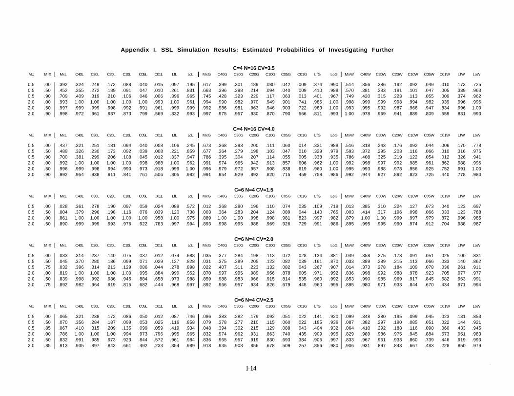
I-141 4
Appendix I. SSL Simulation Results: Estimated Probabilities of Investigating Further
C=4 N=16 CV=3.5MU MIX MxL C40L C30L C20L C10L C05L C01L LfL LoL MxG C40G C30G C20G C10G C05G C01G LfG LoG MxW C40W C30W C20W C10W C05W C01W LfW LoW
0.5 .00 .392 .324 .249 .173 .088 .040 .015 .097 .195 .617 .399 .301 .189 .080 .042 .009 .374 .990 .514 .356 .286 .192 .092 .049 .010 .173 .7250.5 .50 .452 .355 .272 .189 .091 .047 .010 .261 .831 .663 .396 .298 .214 .094 .040 .009 .410 .988 .570 .381 .283 .191 .101 .047 .005 .339 .9630.5 .90 .709 .409 .319 .210 .106 .046 .006 .396 .965 .745 .428 .323 .229 .117 .063 .013 .401 .967 .749 .420 .315 .223 .113 .055 .009 .374 .9622.0 .00 .993 1.00 1.00 1.00 1.00 1.00 .993 1.00 .961 .994 .990 .982 .970 .949 .901 .741 .985 1.00 .998 .999 .999 .998 .994 .982 .939 .996 .9952.0 .50 .997 .999 .999 .998 .992 .991 .961 .999 .999 .992 .986 .981 .963 .946 .903 .722 .983 1.00 .993 .995 .992 .987 .966 .947 .834 .996 1.002.0 .90 .998 .972 .961 .937 .873 .799 .569 .832 .993 .997 .975 .957 .930 .870 .790 .566 .811 .993 1.00 .978 .969 .941 .889 .809 .559 .831 .993
C=4 N=16 CV=4.0MU MIX MxL C40L C30L C20L C10L C05L C01L LfL LoL MxG C40G C30G C20G C10G C05G C01G LfG LoG MxW C40W C30W C20W C10W C05W C01W LfW LoW
0.5 .00 .437 .321 .251 .181 .094 .040 .008 .106 .245 .673 .368 .293 .200 .111 .060 .014 .331 .988 .516 .318 .243 .176 .092 .044 .006 .170 .7780.5 .50 .489 .326 .230 .173 .092 .039 .008 .221 .859 .677 .364 .279 .198 .103 .047 .010 .329 .979 .593 .372 .295 .203 .116 .066 .010 .316 .9750.5 .90 .700 .381 .299 .206 .108 .045 .012 .337 .947 .786 .395 .304 .207 .114 .055 .005 .338 .935 .786 .408 .325 .219 .122 .054 .012 .326 .9412.0 .00 .992 1.00 1.00 1.00 1.00 .998 .988 1.00 .962 .991 .974 .965 .942 .913 .857 .606 .962 1.00 .992 .998 .997 .992 .985 .961 .862 .988 .9952.0 .50 .996 .999 .998 .994 .990 .973 .918 .999 1.00 .996 .979 .972 .957 .908 .838 .619 .960 1.00 .995 .993 .988 .978 .956 .925 .752 .991 1.002.0 .90 .992 .954 .938 .911 .841 .761 .506 .805 .982 .991 .954 .929 .892 .820 .715 .459 .758 .986 .992 .944 .927 .892 .823 .725 .440 .778 .980
C=6 N=4 CV=1.5MU MIX MxL C40L C30L C20L C10L C05L C01L LfL LoL MxG C40G C30G C20G C10G C05G C01G LfG LoG MxW C40W C30W C20W C10W C05W C01W LfW LoW
0.5 .00 .028 .361 .278 .190 .097 .059 .024 .089 .572 .012 .368 .280 .196 .110 .074 .035 .109 .719 .013 .385 .310 .224 .127 .073 .040 .123 .6970.5 .50 .004 .379 .296 .198 .116 .076 .039 .120 .738 .003 .364 .283 .204 .124 .089 .044 .140 .765 .003 .414 .317 .196 .098 .066 .033 .123 .7882.0 .00 .861 1.00 1.00 1.00 1.00 1.00 .958 1.00 .975 .889 1.00 1.00 .998 .998 .981 .823 .997 .982 .879 1.00 1.00 .999 .997 .979 .872 .996 .9852.0 .50 .890 .999 .999 .993 .976 .922 .783 .997 .994 .893 .998 .995 .988 .969 .926 .729 .991 .986 .895 .995 .995 .990 .974 .912 .704 .988 .987
C=6 N=4 CV=2.0MU MIX MxL C40L C30L C20L C10L C05L C01L LfL LoL MxG C40G C30G C20G C10G C05G C01G LfG LoG MxW C40W C30W C20W C10W C05W C01W LfW LoW
0.5 .00 .033 .314 .237 .140 .075 .037 .012 .074 .688 .035 .377 .284 .198 .113 .072 .028 .134 .881 .049 .358 .275 .178 .091 .051 .025 .100 .8310.5 .50 .045 .370 .280 .186 .099 .071 .029 .127 .828 .031 .375 .289 .205 .123 .082 .039 .161 .870 .033 .389 .289 .215 .113 .066 .033 .140 .8620.5 .75 .032 .396 .314 .213 .129 .086 .044 .278 .898 .022 .407 .311 .223 .132 .082 .043 .267 .907 .014 .373 .278 .184 .109 .078 .036 .261 .9112.0 .00 .819 1.00 1.00 1.00 1.00 .995 .884 .999 .952 .870 .997 .995 .989 .956 .878 .605 .971 .992 .836 .998 .992 .988 .978 .923 .705 .977 .9772.0 .50 .839 .998 .992 .986 .945 .884 .658 .973 .988 .859 .988 .983 .966 .915 .814 .535 .960 .992 .853 .990 .985 .969 .917 .845 .582 .963 .9912.0 .75 .892 .982 .964 .919 .815 .682 .444 .968 .997 .892 .966 .957 .934 .826 .679 .445 .960 .995 .895 .980 .971 .933 .844 .670 .434 .971 .994
C=6 N=4 CV=2.5MU MIX MxL C40L C30L C20L C10L C05L C01L LfL LoL MxG C40G C30G C20G C10G C05G C01G LfG LoG MxW C40W C30W C20W C10W C05W C01W LfW LoW
0.5 .00 .065 .321 .238 .172 .086 .050 .012 .087 .746 .086 .383 .282 .179 .092 .051 .022 .141 .920 .099 .348 .280 .195 .099 .045 .023 .131 .8530.5 .50 .070 .356 .284 .187 .099 .053 .025 .116 .858 .079 .378 .277 .210 .115 .060 .022 .185 .936 .087 .382 .297 .190 .085 .051 .022 .144 .9210.5 .85 .067 .410 .315 .209 .135 .099 .059 .419 .934 .048 .394 .302 .215 .129 .088 .043 .404 .932 .064 .410 .292 .188 .116 .090 .060 .433 .9452.0 .00 .786 1.00 1.00 1.00 .994 .973 .796 .995 .965 .832 .974 .962 .931 .863 .740 .435 .909 .995 .829 .989 .986 .975 .945 .884 .573 .951 .9832.0 .50 .832 .991 .985 .973 .923 .844 .572 .961 .984 .836 .965 .957 .919 .830 .693 .384 .906 .997 .833 .967 .961 .933 .860 .739 .446 .919 .9932.0 .85 .913 .935 .897 .843 .661 .492 .233 .854 .989 .918 .935 .908 .856 .678 .509 .257 .856 .980 .906 .931 .897 .843 .667 .483 .228 .850 .979

I-151 5
Appendix I. SSL Simulation Results: Estimated Probabilities of Investigating Further
C=6 N=4 CV=3.0MU MIX MxL C40L C30L C20L C10L C05L C01L LfL LoL MxG C40G C30G C20G C10G C05G C01G LfG LoG MxW C40W C30W C20W C10W C05W C01W LfW LoW
0.5 .00 .081 .307 .244 .169 .090 .041 .011 .097 .766 .124 .346 .259 .160 .074 .038 .013 .144 .970 .099 .318 .241 .172 .075 .037 .008 .117 .8790.5 .50 .113 .371 .301 .210 .111 .051 .016 .137 .893 .145 .385 .290 .195 .097 .057 .022 .206 .967 .131 .375 .295 .184 .102 .054 .019 .167 .9410.5 .85 .126 .366 .277 .189 .090 .052 .023 .333 .955 .125 .373 .290 .185 .096 .052 .030 .358 .955 .123 .388 .283 .190 .089 .059 .023 .346 .9702.0 .00 .766 .997 .994 .991 .972 .936 .726 .979 .958 .827 .942 .923 .879 .779 .629 .272 .862 .992 .784 .977 .964 .941 .889 .788 .452 .918 .9802.0 .50 .788 .977 .964 .947 .874 .777 .471 .933 .988 .831 .928 .908 .861 .759 .599 .279 .860 .998 .793 .939 .913 .888 .789 .674 .361 .873 .9872.0 .85 .847 .894 .857 .815 .658 .445 .190 .843 .981 .860 .912 .882 .810 .654 .440 .184 .850 .982 .849 .893 .853 .797 .643 .462 .201 .825 .988
C=6 N=4 CV=3.5MU MIX MxL C40L C30L C20L C10L C05L C01L LfL LoL MxG C40G C30G C20G C10G C05G C01G LfG LoG MxW C40W C30W C20W C10W C05W C01W LfW LoW
0.5 .00 .109 .303 .241 .177 .084 .034 .008 .098 .787 .159 .332 .269 .168 .074 .033 .014 .180 .971 .144 .360 .281 .202 .120 .053 .009 .147 .9130.5 .50 .120 .322 .245 .166 .097 .046 .013 .125 .905 .163 .336 .266 .175 .076 .037 .006 .183 .969 .153 .353 .275 .184 .084 .047 .012 .165 .9610.5 .90 .187 .397 .293 .199 .093 .047 .022 .392 .912 .179 .402 .276 .175 .063 .029 .013 .376 .923 .172 .367 .279 .171 .065 .037 .016 .376 .9232.0 .00 .761 .996 .992 .981 .957 .896 .626 .961 .963 .780 .883 .850 .796 .676 .524 .199 .775 .997 .739 .956 .941 .905 .815 .711 .365 .846 .9782.0 .50 .799 .975 .963 .939 .865 .746 .445 .913 .990 .801 .893 .861 .812 .674 .479 .180 .825 .997 .794 .903 .887 .844 .744 .590 .275 .828 .9902.0 .90 .855 .858 .827 .738 .550 .365 .143 .692 .925 .834 .840 .808 .736 .569 .356 .122 .713 .916 .832 .840 .799 .736 .524 .338 .089 .689 .923
C=6 N=4 CV=4.0MU MIX MxL C40L C30L C20L C10L C05L C01L LfL LoL MxG C40G C30G C20G C10G C05G C01G LfG LoG MxW C40W C30W C20W C10W C05W C01W LfW LoW
0.5 .00 .104 .296 .232 .165 .093 .041 .012 .107 .809 .212 .337 .277 .179 .087 .046 .010 .209 .970 .148 .331 .250 .184 .104 .044 .011 .144 .9130.5 .50 .118 .278 .222 .149 .091 .048 .012 .124 .892 .227 .365 .286 .201 .093 .042 .009 .234 .974 .187 .366 .270 .177 .092 .041 .014 .186 .9630.5 .90 .226 .361 .282 .179 .076 .031 .014 .337 .923 .248 .383 .273 .174 .079 .037 .012 .324 .909 .243 .383 .296 .189 .074 .034 .015 .340 .9142.0 .00 .763 .991 .988 .973 .935 .864 .588 .938 .971 .761 .839 .806 .758 .642 .453 .150 .760 .996 .751 .936 .914 .874 .771 .639 .300 .820 .9772.0 .50 .745 .956 .941 .901 .819 .681 .357 .870 .988 .731 .817 .775 .714 .572 .388 .129 .721 .992 .761 .895 .864 .818 .699 .543 .222 .800 .9902.0 .90 .802 .823 .778 .698 .532 .362 .124 .683 .927 .767 .778 .744 .675 .499 .302 .069 .669 .911 .768 .791 .746 .680 .518 .323 .082 .675 .927
C=6 N=6 CV=1.5MU MIX MxL C40L C30L C20L C10L C05L C01L LfL LoL MxG C40G C30G C20G C10G C05G C01G LfG LoG MxW C40W C30W C20W C10W C05W C01W LfW LoW
0.5 .00 .025 .354 .267 .180 .089 .045 .015 .091 .218 .016 .392 .301 .208 .112 .056 .023 .115 .408 .021 .387 .294 .190 .095 .053 .017 .098 .3520.5 .50 .014 .402 .309 .212 .119 .062 .034 .151 .457 .008 .392 .291 .200 .118 .079 .028 .152 .542 .005 .397 .305 .219 .116 .071 .023 .140 .5472.0 .00 .924 1.00 1.00 1.00 1.00 1.00 1.00 1.00 .954 .962 1.00 1.00 1.00 1.00 .998 .976 1.00 .985 .960 1.00 1.00 1.00 1.00 .999 .989 1.00 .9822.0 .50 .965 1.00 .999 .999 .996 .991 .928 1.00 .996 .963 1.00 .998 .997 .996 .986 .905 .998 .996 .958 .999 .999 .998 .994 .988 .903 .998 .992
C=6 N=6 CV=2.0MU MIX MxL C40L C30L C20L C10L C05L C01L LfL LoL MxG C40G C30G C20G C10G C05G C01G LfG LoG MxW C40W C30W C20W C10W C05W C01W LfW LoW
0.5 .00 .065 .342 .265 .184 .091 .048 .015 .093 .346 .067 .392 .297 .212 .111 .055 .022 .138 .720 .075 .397 .305 .206 .102 .054 .016 .110 .5810.5 .50 .057 .356 .266 .182 .094 .052 .013 .125 .626 .055 .409 .308 .200 .107 .055 .016 .166 .768 .062 .374 .294 .202 .097 .053 .014 .157 .7700.5 .75 .035 .387 .302 .198 .105 .062 .023 .359 .857 .033 .378 .285 .214 .110 .067 .026 .379 .848 .026 .367 .289 .206 .111 .071 .030 .342 .8642.0 .00 .934 1.00 1.00 1.00 1.00 .999 .990 1.00 .968 .945 1.00 .997 .995 .990 .971 .853 .991 .987 .940 1.00 1.00 .999 .997 .993 .916 .998 .9792.0 .50 .956 .998 .998 .998 .994 .981 .861 .999 .992 .958 .998 .996 .993 .978 .945 .792 .990 .995 .956 .997 .995 .993 .980 .953 .792 .990 .9972.0 .75 .965 .995 .989 .974 .952 .897 .650 .995 1.00 .972 .994 .993 .979 .947 .881 .652 .993 .997 .963 .993 .985 .977 .940 .872 .618 .991 1.00

I-161 6
Appendix I. SSL Simulation Results: Estimated Probabilities of Investigating Further
C=6 N=6 CV=2.5MU MIX MxL C40L C30L C20L C10L C05L C01L LfL LoL MxG C40G C30G C20G C10G C05G C01G LfG LoG MxW C40W C30W C20W C10W C05W C01W LfW LoW
0.5 .00 .114 .371 .299 .200 .103 .056 .011 .111 .468 .115 .372 .286 .200 .106 .052 .017 .167 .848 .128 .352 .268 .193 .102 .052 .015 .119 .7150.5 .50 .109 .334 .235 .171 .079 .037 .009 .119 .702 .142 .366 .296 .208 .102 .053 .018 .213 .919 .127 .366 .269 .199 .099 .048 .019 .177 .8430.5 .85 .091 .394 .298 .190 .101 .056 .027 .526 .965 .084 .390 .284 .186 .100 .061 .027 .524 .954 .085 .418 .324 .227 .113 .065 .026 .529 .9572.0 .00 .909 1.00 1.00 1.00 1.00 .997 .964 1.00 .956 .919 .989 .985 .976 .942 .901 .684 .965 .993 .914 .997 .994 .990 .980 .959 .828 .982 .9812.0 .50 .919 .998 .998 .998 .986 .966 .842 .992 .982 .936 .991 .984 .972 .933 .866 .630 .974 .998 .935 .993 .991 .978 .952 .915 .700 .981 .9932.0 .85 .963 .966 .948 .920 .828 .701 .378 .933 .993 .974 .975 .956 .920 .841 .728 .378 .938 .998 .970 .963 .943 .915 .831 .718 .366 .929 .996
C=6 N=6 CV=3.0MU MIX MxL C40L C30L C20L C10L C05L C01L LfL LoL MxG C40G C30G C20G C10G C05G C01G LfG LoG MxW C40W C30W C20W C10W C05W C01W LfW LoW
0.5 .00 .116 .327 .256 .172 .092 .051 .008 .108 .532 .187 .365 .285 .195 .088 .041 .011 .202 .944 .198 .373 .292 .205 .106 .047 .006 .138 .7980.5 .50 .145 .351 .275 .188 .097 .047 .009 .136 .777 .195 .395 .314 .204 .101 .050 .009 .232 .952 .192 .368 .283 .190 .094 .045 .011 .186 .9250.5 .85 .174 .378 .300 .204 .094 .052 .017 .424 .979 .180 .364 .287 .188 .090 .052 .015 .441 .985 .186 .410 .313 .198 .089 .038 .013 .469 .9882.0 .00 .890 1.00 .999 .999 .996 .992 .933 .996 .957 .918 .968 .960 .933 .881 .807 .513 .924 .996 .911 .990 .985 .981 .957 .919 .699 .965 .9872.0 .50 .909 1.00 .997 .988 .970 .931 .744 .983 .983 .909 .965 .948 .925 .859 .774 .479 .937 1.00 .918 .990 .982 .968 .923 .857 .579 .970 .9942.0 .85 .938 .954 .933 .889 .794 .679 .346 .916 .995 .936 .942 .925 .883 .790 .660 .322 .902 .993 .937 .944 .924 .895 .810 .670 .326 .916 .999
C=6 N=6 CV=3.5MU MIX MxL C40L C30L C20L C10L C05L C01L LfL LoL MxG C40G C30G C20G C10G C05G C01G LfG LoG MxW C40W C30W C20W C10W C05W C01W LfW LoW
0.5 .00 .138 .319 .255 .185 .101 .045 .009 .107 .573 .226 .353 .262 .162 .077 .037 .007 .200 .965 .214 .367 .294 .206 .102 .045 .008 .143 .8410.5 .50 .169 .323 .259 .180 .095 .049 .007 .137 .798 .250 .362 .284 .201 .099 .039 .007 .259 .964 .244 .355 .289 .199 .110 .048 .008 .203 .9230.5 .90 .261 .375 .297 .200 .100 .051 .011 .416 .977 .270 .401 .303 .200 .088 .039 .011 .424 .985 .278 .422 .330 .204 .100 .052 .014 .449 .9722.0 .00 .888 .999 .998 .997 .995 .991 .889 .995 .964 .886 .938 .922 .896 .801 .700 .374 .886 .997 .886 .979 .974 .957 .911 .858 .604 .927 .9802.0 .50 .897 .991 .988 .976 .949 .902 .690 .972 .982 .907 .951 .932 .896 .809 .692 .367 .911 .996 .874 .960 .941 .916 .864 .778 .486 .920 .9942.0 .90 .944 .917 .887 .832 .708 .549 .197 .819 .982 .954 .923 .894 .837 .700 .533 .187 .827 .989 .940 .916 .886 .832 .710 .563 .192 .817 .982
C=6 N=6 CV=4.0MU MIX MxL C40L C30L C20L C10L C05L C01L LfL LoL MxG C40G C30G C20G C10G C05G C01G LfG LoG MxW C40W C30W C20W C10W C05W C01W LfW LoW
0.5 .00 .157 .300 .235 .175 .096 .053 .006 .103 .594 .310 .380 .285 .202 .089 .040 .003 .253 .980 .216 .361 .280 .186 .085 .034 .005 .133 .8770.5 .50 .192 .316 .249 .177 .105 .055 .008 .143 .835 .294 .377 .306 .204 .097 .043 .008 .270 .985 .221 .322 .250 .171 .076 .033 .006 .181 .9440.5 .90 .310 .382 .289 .193 .099 .057 .012 .390 .979 .338 .370 .289 .193 .084 .042 .008 .340 .969 .342 .388 .288 .184 .067 .027 .006 .359 .9692.0 .00 .883 .998 .998 .996 .990 .971 .837 .991 .954 .871 .915 .891 .857 .753 .621 .298 .866 .998 .856 .972 .961 .942 .886 .808 .516 .912 .9792.0 .50 .866 .980 .969 .948 .906 .848 .582 .940 .987 .881 .901 .876 .830 .731 .591 .245 .851 .999 .877 .953 .936 .902 .834 .734 .405 .907 .9932.0 .90 .906 .878 .857 .789 .671 .518 .183 .780 .979 .892 .872 .835 .783 .664 .500 .176 .771 .971 .904 .883 .854 .802 .671 .502 .180 .768 .983
C=6 N=9 CV=1.5MU MIX MxL C40L C30L C20L C10L C05L C01L LfL LoL MxG C40G C30G C20G C10G C05G C01G LfG LoG MxW C40W C30W C20W C10W C05W C01W LfW LoW
0.5 .00 .047 .383 .295 .203 .112 .066 .010 .115 .036 .010 .402 .298 .201 .109 .062 .017 .117 .149 .026 .387 .292 .195 .095 .046 .013 .098 .1110.5 .50 .016 .399 .299 .194 .105 .054 .012 .153 .282 .006 .388 .296 .194 .102 .048 .015 .178 .363 .007 .376 .310 .222 .114 .062 .012 .170 .3812.0 .00 .980 1.00 1.00 1.00 1.00 1.00 1.00 1.00 .963 .995 1.00 1.00 1.00 1.00 1.00 1.00 1.00 .993 .987 1.00 1.00 1.00 1.00 1.00 1.00 1.00 .9762.0 .50 .994 1.00 1.00 1.00 1.00 1.00 .995 1.00 .992 .989 1.00 1.00 1.00 1.00 1.00 .997 1.00 .994 .996 1.00 1.00 1.00 1.00 1.00 .992 1.00 .997

I-171 7
Appendix I. SSL Simulation Results: Estimated Probabilities of Investigating Further.
C=6 N=9 CV=2.0MU MIX MxL C40L C30L C20L C10L C05L C01L LfL LoL MxG C40G C30G C20G C10G C05G C01G LfG LoG MxW C40W C30W C20W C10W C05W C01W LfW LoW
0.5 .00 .119 .382 .297 .210 .107 .061 .010 .108 .140 .088 .368 .276 .196 .110 .067 .017 .147 .534 .077 .363 .267 .173 .090 .048 .009 .097 .3230.5 .50 .088 .395 .299 .198 .097 .060 .013 .157 .497 .065 .386 .295 .196 .100 .056 .011 .198 .657 .076 .397 .305 .185 .094 .050 .010 .201 .6560.5 .75 .057 .408 .316 .218 .117 .063 .012 .529 .852 .049 .391 .286 .182 .097 .050 .014 .497 .843 .042 .367 .274 .182 .097 .055 .021 .538 .8872.0 .00 .980 1.00 1.00 1.00 1.00 1.00 .999 1.00 .973 .988 1.00 1.00 1.00 1.00 .999 .984 1.00 .996 .982 1.00 1.00 1.00 1.00 .999 .997 1.00 .9872.0 .50 .987 1.00 1.00 1.00 1.00 .999 .983 1.00 .988 .986 1.00 .999 .999 .993 .989 .949 1.00 .997 .987 1.00 1.00 1.00 .998 .996 .969 1.00 .9942.0 .75 .991 .998 .996 .993 .987 .971 .873 1.00 .999 .993 .996 .996 .996 .992 .977 .876 .997 .999 .998 .998 .996 .994 .987 .972 .871 1.00 1.00
C=6 N=9 CV=2.5MU MIX MxL C40L C30L C20L C10L C05L C01L LfL LoL MxG C40G C30G C20G C10G C05G C01G LfG LoG MxW C40W C30W C20W C10W C05W C01W LfW LoW
0.5 .00 .136 .351 .272 .180 .097 .050 .014 .107 .225 .189 .391 .287 .199 .093 .045 .008 .187 .820 .180 .351 .281 .184 .086 .047 .006 .110 .5430.5 .50 .146 .362 .284 .195 .110 .065 .011 .167 .605 .179 .392 .316 .216 .111 .052 .009 .273 .882 .176 .375 .291 .199 .104 .057 .012 .201 .8100.5 .85 .114 .363 .290 .199 .099 .055 .016 .658 .992 .136 .368 .292 .189 .098 .054 .009 .660 .986 .133 .402 .304 .208 .084 .050 .011 .670 .9882.0 .00 .977 1.00 1.00 1.00 1.00 1.00 .999 1.00 .969 .986 .997 .996 .995 .992 .983 .912 .994 .997 .974 1.00 1.00 1.00 1.00 .997 .958 1.00 .9842.0 .50 .980 1.00 1.00 1.00 1.00 .996 .957 1.00 .994 .984 .998 .997 .992 .978 .955 .851 .995 .999 .985 1.00 .999 .995 .990 .981 .897 .997 1.002.0 .85 .994 .991 .985 .967 .937 .877 .631 .972 1.00 .992 .991 .987 .975 .943 .885 .669 .982 1.00 .995 .991 .985 .975 .942 .886 .648 .980 1.00
C=6 N=9 CV=3.0MU MIX MxL C40L C30L C20L C10L C05L C01L LfL LoL MxG C40G C30G C20G C10G C05G C01G LfG LoG MxW C40W C30W C20W C10W C05W C01W LfW LoW
0.5 .00 .199 .346 .261 .188 .096 .049 .008 .111 .320 .286 .386 .294 .195 .112 .054 .008 .256 .933 .229 .368 .279 .180 .081 .043 .007 .116 .6550.5 .50 .204 .366 .283 .203 .109 .051 .011 .171 .664 .278 .393 .303 .196 .109 .051 .009 .309 .955 .255 .376 .285 .176 .092 .050 .008 .206 .8880.5 .85 .247 .394 .300 .199 .099 .045 .010 .583 .992 .266 .389 .314 .214 .103 .058 .007 .575 .996 .268 .409 .323 .214 .090 .049 .007 .562 .9942.0 .00 .964 1.00 1.00 1.00 1.00 1.00 .994 1.00 .949 .972 .991 .987 .978 .962 .931 .787 .974 .995 .966 1.00 1.00 1.00 .996 .984 .921 .996 .9852.0 .50 .978 1.00 1.00 .999 .996 .985 .929 1.00 .991 .973 .989 .984 .980 .956 .905 .741 .984 1.00 .978 .996 .994 .987 .966 .933 .813 .989 .9992.0 .85 .988 .978 .969 .947 .907 .846 .611 .963 .999 .990 .984 .972 .958 .915 .840 .581 .963 .997 .986 .979 .968 .953 .907 .842 .588 .962 1.00
C=6 N=9 CV=3.5MU MIX MxL C40L C30L C20L C10L C05L C01L LfL LoL MxG C40G C30G C20G C10G C05G C01G LfG LoG MxW C40W C30W C20W C10W C05W C01W LfW LoW
0.5 .00 .224 .368 .289 .202 .092 .046 .004 .099 .380 .369 .402 .305 .198 .112 .064 .018 .289 .966 .265 .337 .257 .174 .092 .049 .008 .131 .7120.5 .50 .239 .354 .283 .191 .109 .054 .007 .180 .731 .342 .374 .288 .189 .091 .048 .006 .306 .977 .305 .372 .289 .202 .099 .051 .012 .233 .9200.5 .90 .351 .394 .299 .203 .090 .035 .003 .509 .984 .376 .403 .306 .211 .105 .057 .011 .498 .987 .368 .420 .310 .208 .098 .049 .008 .497 .9872.0 .00 .958 1.00 1.00 1.00 1.00 .999 .989 1.00 .959 .970 .986 .976 .958 .914 .852 .633 .967 .996 .963 .996 .995 .992 .982 .952 .841 .988 .9932.0 .50 .958 .996 .992 .990 .985 .965 .889 .991 .989 .972 .980 .971 .954 .911 .838 .601 .970 .998 .967 .996 .991 .984 .960 .903 .719 .988 .9982.0 .90 .985 .966 .951 .911 .827 .710 .402 .885 .996 .990 .973 .958 .925 .845 .743 .427 .894 .998 .984 .949 .924 .884 .798 .689 .387 .847 .996

I-181 8
Appendix I. SSL Simulation Results: Estimated Probabilities of Investigating Further
C=6 N=9 CV=4.0MU MIX MxL C40L C30L C20L C10L C05L C01L LfL LoL MxG C40G C30G C20G C10G C05G C01G LfG LoG MxW C40W C30W C20W C10W C05W C01W LfW LoW
0.5 .00 .217 .314 .241 .171 .082 .036 .007 .093 .393 .392 .367 .299 .207 .100 .044 .009 .302 .977 .295 .342 .264 .194 .101 .045 .005 .160 .7630.5 .50 .267 .328 .249 .185 .088 .044 .005 .153 .758 .394 .350 .262 .184 .106 .050 .008 .310 .989 .338 .353 .270 .197 .108 .048 .006 .236 .9380.5 .90 .430 .380 .297 .207 .113 .056 .013 .446 .987 .484 .420 .333 .222 .095 .036 .005 .449 .974 .459 .397 .296 .195 .091 .040 .011 .417 .9822.0 .00 .960 1.00 1.00 .999 .997 .993 .969 .996 .965 .954 .962 .952 .929 .867 .772 .498 .942 .998 .956 .996 .990 .986 .973 .937 .780 .978 .9812.0 .50 .963 .999 .998 .995 .980 .961 .844 .990 .993 .957 .955 .945 .927 .862 .767 .509 .946 .999 .956 .988 .981 .960 .922 .857 .638 .962 .9982.0 .90 .963 .942 .916 .880 .795 .688 .394 .863 .996 .968 .947 .926 .880 .784 .646 .351 .851 .993 .965 .941 .920 .877 .779 .661 .343 .849 .993
C=6 N=12 CV=1.5MU MIX MxL C40L C30L C20L C10L C05L C01L LfL LoL MxG C40G C30G C20G C10G C05G C01G LfG LoG MxW C40W C30W C20W C10W C05W C01W LfW LoW
0.5 .00 .070 .392 .305 .208 .102 .052 .014 .108 .008 .020 .369 .279 .177 .086 .042 .008 .104 .042 .030 .362 .294 .188 .098 .046 .010 .111 .0300.5 .50 .029 .386 .297 .202 .103 .060 .012 .178 .228 .012 .404 .316 .204 .120 .064 .018 .193 .285 .007 .403 .299 .192 .104 .058 .017 .187 .2992.0 .00 .997 1.00 1.00 1.00 1.00 1.00 1.00 1.00 .976 1.00 1.00 1.00 1.00 1.00 1.00 1.00 1.00 .993 .995 1.00 1.00 1.00 1.00 1.00 1.00 1.00 .9862.0 .50 .998 1.00 1.00 1.00 1.00 1.00 .999 1.00 .995 1.00 1.00 1.00 1.00 1.00 1.00 1.00 1.00 .998 .999 1.00 1.00 1.00 1.00 1.00 1.00 1.00 .997
C=6 N=12 CV=2.0MU MIX MxL C40L C30L C20L C10L C05L C01L LfL LoL MxG C40G C30G C20G C10G C05G C01G LfG LoG MxW C40W C30W C20W C10W C05W C01W LfW LoW
0.5 .00 .132 .393 .313 .200 .113 .063 .008 .122 .045 .110 .377 .273 .188 .122 .060 .012 .171 .373 .128 .399 .302 .207 .093 .053 .017 .119 .1670.5 .50 .124 .401 .313 .218 .123 .060 .011 .190 .388 .089 .378 .276 .195 .098 .052 .017 .241 .603 .093 .383 .294 .209 .101 .052 .014 .233 .5730.5 .75 .071 .409 .322 .214 .102 .049 .010 .698 .920 .071 .402 .290 .196 .102 .051 .015 .692 .912 .061 .439 .330 .208 .115 .066 .017 .695 .9122.0 .00 .992 1.00 1.00 1.00 1.00 1.00 1.00 1.00 .963 .997 1.00 1.00 1.00 1.00 1.00 .998 1.00 .992 .993 1.00 1.00 1.00 1.00 1.00 1.00 1.00 .9852.0 .50 .998 1.00 1.00 1.00 1.00 1.00 .999 1.00 .996 1.00 1.00 1.00 1.00 1.00 1.00 .995 1.00 .997 .999 1.00 1.00 1.00 1.00 1.00 .996 1.00 .9972.0 .75 1.00 1.00 1.00 1.00 .998 .995 .962 1.00 1.00 1.00 1.00 1.00 1.00 .999 .995 .970 1.00 1.00 .997 1.00 1.00 1.00 .997 .995 .959 1.00 1.00
C=6 N=12 CV=2.5MU MIX MxL C40L C30L C20L C10L C05L C01L LfL LoL MxG C40G C30G C20G C10G C05G C01G LfG LoG MxW C40W C30W C20W C10W C05W C01W LfW LoW
0.5 .00 .199 .361 .284 .199 .110 .053 .012 .117 .098 .251 .395 .305 .222 .105 .054 .012 .243 .744 .210 .371 .289 .212 .104 .044 .011 .134 .3580.5 .50 .222 .377 .279 .187 .112 .054 .013 .182 .502 .252 .419 .330 .222 .110 .068 .009 .331 .837 .258 .390 .303 .228 .122 .063 .016 .268 .7560.5 .85 .163 .405 .307 .203 .097 .045 .012 .770 .998 .143 .400 .297 .187 .089 .045 .012 .789 .994 .155 .393 .301 .208 .095 .056 .014 .773 .9952.0 .00 .989 1.00 1.00 1.00 1.00 1.00 1.00 1.00 .958 .993 1.00 .999 .999 .997 .991 .962 .998 .997 .996 1.00 1.00 1.00 1.00 1.00 .996 1.00 .9872.0 .50 .993 1.00 .999 .999 .999 .998 .990 .999 .995 1.00 .999 .999 .999 .997 .992 .960 .999 .999 .996 1.00 1.00 .999 .997 .993 .969 1.00 1.002.0 .85 .999 .995 .992 .986 .970 .944 .800 .988 .998 1.00 .993 .991 .985 .970 .940 .807 .984 1.00 1.00 .999 .998 .991 .980 .949 .815 .997 1.00
C=6 N=12 CV=3.0MU MIX MxL C40L C30L C20L C10L C05L C01L LfL LoL MxG C40G C30G C20G C10G C05G C01G LfG LoG MxW C40W C30W C20W C10W C05W C01W LfW LoW
0.5 .00 .247 .360 .289 .200 .114 .056 .012 .121 .164 .351 .411 .311 .218 .110 .047 .014 .307 .894 .326 .385 .303 .190 .109 .051 .008 .144 .5500.5 .50 .298 .362 .284 .191 .086 .052 .010 .178 .625 .318 .367 .289 .205 .105 .056 .009 .360 .945 .325 .368 .266 .183 .093 .050 .006 .254 .8640.5 .85 .322 .401 .309 .208 .109 .054 .008 .657 .996 .332 .382 .279 .180 .096 .047 .011 .632 .999 .320 .388 .291 .199 .084 .043 .008 .647 .9992.0 .00 .992 1.00 1.00 1.00 1.00 1.00 .999 1.00 .975 .991 1.00 .998 .993 .986 .972 .904 .999 .999 .992 1.00 1.00 .999 .998 .996 .981 .999 .9892.0 .50 .989 .999 .998 .997 .997 .995 .984 .999 .991 .995 .999 .997 .994 .983 .966 .875 .996 1.00 .993 .997 .997 .996 .993 .986 .938 .996 .9992.0 .85 .994 .992 .990 .987 .958 .925 .771 .983 .999 .999 .993 .985 .975 .949 .911 .761 .981 1.00 .997 .992 .984 .975 .941 .908 .760 .982 1.00

I-191 9
Appendix I. SSL Simulation Results: Estimated Probabilities of Investigating Further.
C=6 N=12 CV=3.5MU MIX MxL C40L C30L C20L C10L C05L C01L LfL LoL MxG C40G C30G C20G C10G C05G C01G LfG LoG MxW C40W C30W C20W C10W C05W C01W LfW LoW
0.5 .00 .279 .327 .269 .189 .105 .049 .009 .113 .216 .421 .364 .271 .188 .095 .051 .011 .327 .967 .366 .359 .277 .202 .125 .071 .016 .172 .6310.5 .50 .326 .352 .286 .204 .109 .061 .011 .186 .642 .439 .392 .300 .202 .105 .050 .007 .376 .981 .386 .369 .275 .193 .108 .051 .008 .270 .8990.5 .90 .470 .408 .303 .204 .102 .051 .009 .559 .991 .458 .384 .302 .209 .103 .050 .009 .543 .990 .449 .384 .286 .196 .090 .049 .011 .502 .9882.0 .00 .988 1.00 1.00 1.00 1.00 1.00 .999 1.00 .963 .991 .997 .995 .985 .971 .934 .778 .990 1.00 .977 1.00 .999 .996 .989 .984 .938 .993 .9892.0 .50 .992 1.00 1.00 1.00 .999 .996 .968 1.00 .993 .992 .992 .988 .984 .970 .936 .796 .989 1.00 .993 .996 .995 .992 .980 .969 .878 .992 .9972.0 .90 .998 .975 .969 .953 .885 .818 .570 .933 .995 .997 .981 .972 .936 .887 .807 .563 .914 .999 .996 .975 .965 .939 .891 .812 .572 .920 .999
C=6 N=12 CV=4.0MU MIX MxL C40L C30L C20L C10L C05L C01L LfL LoL MxG C40G C30G C20G C10G C05G C01G LfG LoG MxW C40W C30W C20W C10W C05W C01W LfW LoW
0.5 .00 .286 .333 .254 .169 .085 .035 .004 .092 .242 .506 .390 .295 .199 .095 .047 .008 .353 .988 .365 .322 .259 .173 .081 .040 .008 .152 .6960.5 .50 .313 .331 .251 .171 .087 .044 .012 .166 .696 .550 .415 .336 .231 .108 .058 .011 .402 .994 .438 .371 .285 .196 .099 .051 .008 .273 .9280.5 .90 .511 .388 .301 .210 .118 .053 .016 .487 .987 .586 .401 .309 .220 .122 .057 .008 .465 .988 .564 .408 .297 .203 .089 .049 .009 .463 .9732.0 .00 .982 1.00 1.00 1.00 1.00 1.00 .996 1.00 .962 .985 .983 .975 .956 .927 .879 .676 .974 1.00 .978 .997 .995 .994 .985 .968 .889 .992 .9902.0 .50 .988 .999 .999 .998 .995 .989 .934 .998 .990 .981 .978 .969 .953 .910 .843 .643 .975 1.00 .987 .994 .992 .983 .969 .937 .800 .989 .9982.0 .90 .993 .974 .962 .939 .878 .791 .559 .913 .999 .991 .965 .941 .919 .858 .762 .498 .899 .996 .995 .972 .958 .928 .861 .778 .506 .901 1.00
C=6 N=16 CV=1.5MU MIX MxL C40L C30L C20L C10L C05L C01L LfL LoL MxG C40G C30G C20G C10G C05G C01G LfG LoG MxW C40W C30W C20W C10W C05W C01W LfW LoW
0.5 .00 .084 .393 .302 .206 .104 .062 .006 .111 .000 .042 .398 .296 .197 .100 .049 .012 .121 .015 .044 .396 .314 .213 .104 .057 .009 .124 .0040.5 .50 .033 .410 .305 .212 .112 .060 .012 .206 .214 .022 .373 .292 .184 .097 .057 .015 .228 .284 .010 .395 .301 .185 .098 .036 .011 .224 .2882.0 .00 .999 1.00 1.00 1.00 1.00 1.00 1.00 1.00 .977 1.00 1.00 1.00 1.00 1.00 1.00 1.00 1.00 .996 1.00 1.00 1.00 1.00 1.00 1.00 1.00 1.00 .9922.0 .50 1.00 1.00 1.00 1.00 1.00 1.00 1.00 1.00 .997 1.00 1.00 1.00 1.00 1.00 1.00 1.00 1.00 1.00 1.00 1.00 1.00 1.00 1.00 1.00 1.00 1.00 .999
C=6 N=16 CV=2.0MU MIX MxL C40L C30L C20L C10L C05L C01L LfL LoL MxG C40G C30G C20G C10G C05G C01G LfG LoG MxW C40W C30W C20W C10W C05W C01W LfW LoW
0.5 .00 .180 .373 .284 .195 .112 .061 .014 .117 .011 .138 .403 .315 .220 .107 .056 .013 .190 .221 .182 .394 .308 .201 .107 .060 .016 .140 .0660.5 .50 .168 .406 .315 .216 .104 .058 .017 .213 .292 .134 .370 .269 .198 .104 .058 .014 .299 .572 .143 .399 .297 .199 .103 .065 .013 .303 .5220.5 .75 .086 .414 .302 .215 .118 .060 .020 .838 .946 .066 .385 .289 .194 .105 .053 .017 .815 .956 .063 .409 .315 .218 .094 .052 .016 .812 .9422.0 .00 1.00 1.00 1.00 1.00 1.00 1.00 1.00 1.00 .972 1.00 1.00 1.00 1.00 1.00 1.00 1.00 1.00 .999 .999 1.00 1.00 1.00 1.00 1.00 1.00 1.00 .9882.0 .50 1.00 1.00 1.00 1.00 1.00 1.00 1.00 1.00 .998 .999 1.00 1.00 1.00 1.00 1.00 .999 1.00 1.00 1.00 1.00 1.00 1.00 1.00 1.00 1.00 1.00 1.002.0 .75 1.00 1.00 1.00 1.00 1.00 1.00 .996 1.00 1.00 1.00 1.00 1.00 1.00 .999 .999 .996 1.00 1.00 1.00 1.00 1.00 1.00 1.00 1.00 .995 1.00 1.00
C=6 N=16 CV=2.5MU MIX MxL C40L C30L C20L C10L C05L C01L LfL LoL MxG C40G C30G C20G C10G C05G C01G LfG LoG MxW C40W C30W C20W C10W C05W C01W LfW LoW
0.5 .00 .255 .377 .281 .195 .097 .048 .010 .105 .029 .308 .404 .302 .203 .097 .048 .009 .263 .666 .304 .393 .316 .209 .109 .054 .009 .155 .2190.5 .50 .251 .359 .272 .187 .087 .039 .007 .190 .387 .293 .380 .292 .196 .101 .046 .017 .364 .839 .291 .395 .297 .207 .101 .056 .013 .316 .7170.5 .85 .196 .392 .304 .214 .107 .061 .018 .861 .999 .200 .371 .276 .180 .085 .046 .009 .871 1.00 .225 .433 .330 .225 .129 .074 .015 .869 1.002.0 .00 .996 1.00 1.00 1.00 1.00 1.00 1.00 1.00 .965 .998 1.00 1.00 1.00 1.00 .999 .994 1.00 .999 .999 1.00 1.00 1.00 1.00 1.00 1.00 1.00 .9912.0 .50 1.00 1.00 1.00 1.00 1.00 1.00 .998 1.00 .994 .999 1.00 1.00 1.00 .999 .996 .985 1.00 1.00 .998 1.00 1.00 1.00 .999 .999 .994 1.00 .9982.0 .85 .999 1.00 .999 .999 .994 .986 .944 .999 1.00 .999 1.00 1.00 .998 .991 .985 .927 .997 1.00 1.00 .999 .998 .997 .992 .978 .923 .999 1.00

I-202 0
Appendix I. SSL Simulation Results: Estimated Probabilities of Investigating Further
C=6 N=16 CV=3.0MU MIX MxL C40L C30L C20L C10L C05L C01L LfL LoL MxG C40G C30G C20G C10G C05G C01G LfG LoG MxW C40W C30W C20W C10W C05W C01W LfW LoW
0.5 .00 .318 .369 .287 .198 .105 .048 .009 .112 .065 .434 .394 .304 .199 .100 .053 .009 .374 .896 .397 .381 .295 .201 .112 .071 .014 .175 .4040.5 .50 .338 .356 .281 .196 .098 .052 .010 .209 .515 .434 .408 .308 .202 .093 .051 .011 .448 .954 .439 .381 .305 .214 .103 .053 .011 .328 .8350.5 .85 .418 .407 .298 .205 .107 .052 .012 .772 1.00 .423 .393 .310 .214 .105 .052 .012 .748 1.00 .438 .418 .334 .236 .115 .054 .009 .762 1.002.0 .00 .999 1.00 1.00 1.00 1.00 1.00 .999 1.00 .964 .998 1.00 .998 .997 .996 .993 .967 1.00 1.00 .998 1.00 1.00 1.00 1.00 1.00 .998 1.00 .9922.0 .50 1.00 1.00 1.00 1.00 1.00 1.00 1.00 1.00 .997 .999 .999 .998 .998 .995 .990 .955 1.00 1.00 .998 1.00 1.00 .999 .999 .998 .981 1.00 .9992.0 .85 .998 .998 .996 .993 .985 .970 .895 .996 1.00 1.00 .997 .995 .991 .983 .957 .872 .995 1.00 .999 .999 .997 .991 .978 .958 .882 .997 1.00
C=6 N=16 CV=3.5MU MIX MxL C40L C30L C20L C10L C05L C01L LfL LoL MxG C40G C30G C20G C10G C05G C01G LfG LoG MxW C40W C30W C20W C10W C05W C01W LfW LoW
0.5 .00 .347 .347 .287 .201 .112 .052 .007 .126 .102 .547 .405 .297 .207 .112 .056 .011 .417 .968 .437 .386 .306 .217 .111 .056 .015 .192 .5360.5 .50 .392 .360 .286 .206 .099 .060 .011 .206 .569 .563 .394 .297 .218 .135 .071 .015 .458 .983 .491 .382 .287 .215 .101 .056 .017 .326 .9010.5 .90 .563 .390 .275 .185 .105 .050 .006 .607 .991 .546 .403 .301 .213 .109 .055 .017 .615 .998 .539 .383 .296 .198 .108 .055 .007 .608 .9942.0 .00 .993 1.00 1.00 1.00 1.00 1.00 .998 1.00 .962 .999 .999 .999 .996 .987 .974 .899 .998 .999 1.00 1.00 1.00 1.00 1.00 .999 .990 1.00 .9952.0 .50 .999 1.00 1.00 1.00 .999 .997 .989 1.00 .996 .997 .997 .996 .994 .981 .967 .891 .998 1.00 .997 .999 .998 .998 .995 .989 .946 1.00 1.002.0 .90 .998 .989 .982 .977 .945 .911 .751 .956 .999 .999 .995 .990 .976 .945 .907 .726 .954 .998 .998 .986 .980 .969 .944 .912 .727 .958 1.00
C=6 N=16 CV=4.0MU MIX MxL C40L C30L C20L C10L C05L C01L LfL LoL MxG C40G C30G C20G C10G C05G C01G LfG LoG MxW C40W C30W C20W C10W C05W C01W LfW LoW
0.5 .00 .386 .345 .267 .192 .108 .067 .010 .119 .152 .606 .386 .289 .194 .099 .060 .011 .402 .987 .496 .366 .285 .204 .095 .042 .008 .184 .6200.5 .50 .404 .333 .247 .163 .091 .045 .007 .200 .595 .652 .435 .335 .230 .128 .068 .014 .481 .995 .547 .390 .303 .217 .103 .060 .007 .329 .9260.5 .90 .642 .395 .308 .205 .102 .053 .015 .546 .994 .647 .407 .308 .208 .114 .056 .013 .538 .983 .670 .407 .302 .215 .114 .059 .012 .511 .9812.0 .00 .993 1.00 1.00 1.00 1.00 1.00 .999 1.00 .958 .994 .995 .990 .979 .952 .929 .810 .992 1.00 .999 1.00 1.00 .999 .999 .996 .971 .999 .9932.0 .50 1.00 1.00 1.00 1.00 1.00 .999 .990 1.00 1.00 .998 .990 .987 .978 .950 .923 .791 .989 1.00 .996 .999 .998 .998 .989 .974 .901 .997 .9982.0 .90 .998 .986 .981 .960 .927 .872 .703 .945 1.00 .996 .982 .973 .962 .922 .860 .668 .947 .997 .999 .981 .967 .956 .913 .857 .655 .938 .999
C=9 N=4 CV=1.5MU MIX MxL C40L C30L C20L C10L C05L C01L LfL LoL MxG C40G C30G C20G C10G C05G C01G LfG LoG MxW C40W C30W C20W C10W C05W C01W LfW LoW
0.5 .00 .006 .368 .275 .188 .107 .067 .029 .091 .468 .001 .384 .301 .187 .118 .072 .038 .115 .645 .003 .402 .292 .200 .102 .062 .028 .092 .6030.5 .50 .003 .370 .279 .180 .103 .071 .040 .095 .610 .002 .385 .290 .213 .130 .084 .043 .125 .660 .001 .423 .336 .224 .130 .087 .045 .114 .7102.0 .00 .864 1.00 1.00 1.00 1.00 1.00 .981 1.00 .972 .889 1.00 1.00 1.00 .998 .993 .905 .999 .981 .881 1.00 1.00 1.00 1.00 .996 .947 1.00 .9842.0 .50 .903 .999 .998 .998 .996 .984 .910 .998 .985 .905 1.00 .999 .999 .995 .980 .869 .997 .980 .886 1.00 .998 .997 .985 .963 .836 .994 .987
C=9 N=4 CV=2.0MU MIX MxL C40L C30L C20L C10L C05L C01L LfL LoL MxG C40G C30G C20G C10G C05G C01G LfG LoG MxW C40W C30W C20W C10W C05W C01W LfW LoW
0.5 .00 .025 .355 .267 .195 .102 .064 .028 .102 .619 .014 .382 .286 .197 .120 .069 .031 .118 .795 .018 .368 .283 .204 .117 .070 .026 .112 .7160.5 .50 .014 .377 .295 .206 .114 .067 .029 .109 .724 .019 .398 .308 .213 .120 .081 .041 .132 .809 .008 .380 .287 .211 .117 .066 .034 .119 .8030.5 .75 .011 .405 .297 .211 .129 .082 .045 .199 .825 .005 .395 .297 .213 .123 .075 .045 .198 .856 .006 .397 .306 .199 .126 .090 .042 .176 .8342.0 .00 .845 1.00 1.00 1.00 1.00 1.00 .946 1.00 .968 .856 .999 .998 .997 .985 .954 .777 .994 .986 .852 .999 .999 .998 .998 .980 .858 .997 .9822.0 .50 .866 1.00 .999 .999 .990 .967 .828 .995 .987 .869 .997 .995 .993 .982 .934 .723 .990 .984 .879 .998 .995 .989 .969 .930 .722 .981 .9812.0 .75 .906 .993 .983 .975 .932 .856 .662 .994 .991 .903 .993 .989 .974 .924 .828 .644 .989 .993 .885 .991 .985 .974 .915 .814 .598 .988 .994

I-212 1
Appendix I. SSL Simulation Results: Estimated Probabilities of Investigating Further
C=9 N=4 CV=2.5MU MIX MxL C40L C30L C20L C10L C05L C01L LfL LoL MxG C40G C30G C20G C10G C05G C01G LfG LoG MxW C40W C30W C20W C10W C05W C01W LfW LoW
0.5 .00 .053 .344 .265 .188 .107 .060 .022 .109 .683 .028 .379 .279 .184 .082 .051 .023 .111 .877 .061 .384 .303 .212 .107 .065 .029 .118 .8020.5 .50 .037 .359 .286 .198 .103 .056 .022 .102 .806 .039 .374 .284 .199 .101 .051 .019 .144 .902 .056 .390 .312 .202 .095 .054 .024 .130 .8720.5 .85 .018 .366 .280 .201 .101 .060 .030 .344 .910 .014 .367 .276 .187 .107 .071 .045 .344 .897 .021 .411 .313 .230 .135 .088 .043 .390 .9252.0 .00 .824 .999 .999 .999 .999 .994 .910 .999 .970 .857 .994 .990 .984 .956 .871 .604 .968 .994 .811 .999 .998 .992 .976 .928 .720 .980 .9782.0 .50 .820 .998 .995 .990 .975 .914 .717 .984 .983 .873 .992 .986 .978 .930 .843 .583 .967 .992 .844 .992 .985 .977 .941 .863 .618 .966 .9882.0 .85 .895 .976 .967 .924 .824 .620 .359 .973 .992 .881 .975 .956 .908 .807 .642 .402 .968 .997 .908 .976 .951 .922 .812 .651 .373 .968 .998
C=9 N=4 CV=3.0MU MIX MxL C40L C30L C20L C10L C05L C01L LfL LoL MxG C40G C30G C20G C10G C05G C01G LfG LoG MxW C40W C30W C20W C10W C05W C01W LfW LoW
0.5 .00 .065 .333 .259 .190 .111 .066 .025 .116 .728 .084 .380 .301 .200 .095 .042 .015 .153 .917 .074 .354 .280 .184 .091 .045 .015 .106 .8430.5 .50 .065 .342 .270 .186 .095 .054 .020 .115 .840 .077 .376 .291 .195 .095 .046 .013 .166 .936 .084 .373 .284 .202 .112 .059 .022 .155 .9050.5 .85 .074 .409 .297 .194 .101 .063 .029 .336 .945 .080 .406 .309 .194 .106 .064 .031 .336 .958 .064 .361 .269 .180 .103 .069 .040 .333 .9552.0 .00 .810 1.00 1.00 .998 .998 .991 .844 .997 .967 .830 .972 .959 .934 .863 .758 .465 .917 .992 .830 .987 .982 .975 .949 .886 .633 .954 .9832.0 .50 .817 .992 .991 .986 .956 .886 .648 .967 .980 .836 .966 .953 .925 .856 .727 .428 .926 .990 .846 .984 .980 .963 .915 .825 .530 .946 .9912.0 .85 .846 .956 .918 .879 .761 .598 .362 .954 .991 .867 .953 .931 .885 .757 .596 .300 .949 .996 .875 .955 .930 .872 .759 .587 .318 .940 .995
C=9 N=4 CV=3.5MU MIX MxL C40L C30L C20L C10L C05L C01L LfL LoL MxG C40G C30G C20G C10G C05G C01G LfG LoG MxW C40W C30W C20W C10W C05W C01W LfW LoW
0.5 .00 .075 .332 .265 .181 .111 .063 .021 .118 .748 .126 .363 .281 .187 .100 .049 .019 .177 .950 .115 .346 .270 .181 .097 .049 .018 .124 .8610.5 .50 .094 .343 .260 .190 .105 .055 .019 .124 .859 .117 .380 .283 .193 .103 .054 .023 .199 .953 .110 .356 .275 .188 .086 .046 .021 .143 .9030.5 .90 .114 .385 .296 .197 .105 .060 .033 .406 .963 .106 .388 .287 .184 .085 .049 .026 .417 .967 .112 .381 .275 .192 .083 .046 .024 .415 .9652.0 .00 .760 1.00 1.00 .999 .996 .974 .809 .997 .959 .818 .944 .926 .893 .816 .685 .331 .880 .991 .784 .983 .979 .967 .912 .839 .530 .930 .9672.0 .50 .800 .995 .993 .977 .937 .858 .575 .955 .988 .819 .941 .916 .879 .787 .627 .327 .892 .997 .802 .968 .953 .928 .862 .728 .436 .923 .9922.0 .90 .882 .922 .891 .826 .681 .500 .199 .874 .976 .869 .910 .879 .820 .657 .460 .186 .852 .970 .865 .901 .873 .814 .652 .459 .175 .855 .968
C=9 N=4 CV=4.0MU MIX MxL C40L C30L C20L C10L C05L C01L LfL LoL MxG C40G C30G C20G C10G C05G C01G LfG LoG MxW C40W C30W C20W C10W C05W C01W LfW LoW
0.5 .00 .098 .327 .246 .166 .088 .041 .006 .101 .783 .149 .352 .262 .174 .086 .042 .010 .186 .962 .131 .326 .260 .172 .077 .035 .006 .108 .9050.5 .50 .102 .343 .259 .174 .097 .053 .017 .114 .872 .152 .368 .281 .184 .092 .043 .019 .207 .971 .125 .350 .267 .187 .088 .042 .010 .155 .9430.5 .90 .151 .375 .282 .192 .091 .060 .027 .366 .963 .159 .394 .307 .194 .102 .058 .026 .383 .963 .149 .365 .278 .179 .082 .043 .024 .379 .9692.0 .00 .754 1.00 .999 .994 .985 .959 .738 .990 .958 .798 .913 .882 .848 .741 .592 .258 .842 .995 .764 .973 .960 .931 .862 .774 .443 .889 .9822.0 .50 .780 .982 .976 .951 .904 .826 .530 .934 .981 .773 .898 .862 .816 .702 .554 .247 .830 .994 .776 .938 .909 .880 .797 .657 .323 .845 .9872.0 .90 .797 .872 .835 .765 .620 .430 .164 .831 .978 .832 .872 .835 .779 .632 .434 .172 .822 .971 .841 .890 .847 .794 .618 .420 .165 .838 .983
C=9 N=6 CV=1.5MU MIX MxL C40L C30L C20L C10L C05L C01L LfL LoL MxG C40G C30G C20G C10G C05G C01G LfG LoG MxW C40W C30W C20W C10W C05W C01W LfW LoW
0.5 .00 .013 .366 .275 .180 .093 .045 .018 .088 .112 .003 .412 .303 .207 .114 .071 .024 .113 .240 .006 .380 .295 .199 .099 .062 .025 .097 .1850.5 .50 .007 .403 .302 .204 .107 .059 .017 .117 .293 .001 .404 .324 .220 .120 .072 .025 .120 .302 .001 .390 .292 .200 .103 .062 .024 .104 .3332.0 .00 .944 1.00 1.00 1.00 1.00 1.00 1.00 1.00 .964 .964 1.00 1.00 1.00 1.00 .999 .994 1.00 .988 .969 1.00 1.00 1.00 1.00 1.00 .997 1.00 .9852.0 .50 .963 1.00 1.00 1.00 1.00 1.00 .991 1.00 .990 .976 1.00 1.00 1.00 1.00 .997 .974 1.00 .995 .973 1.00 1.00 1.00 1.00 .998 .969 1.00 .997

I-222 2
Appendix I. SSL Simulation Results: Estimated Probabilities of Investigating Further
C=9 N=6 CV=2.0MU MIX MxL C40L C30L C20L C10L C05L C01L LfL LoL MxG C40G C30G C20G C10G C05G C01G LfG LoG MxW C40W C30W C20W C10W C05W C01W LfW LoW
0.5 .00 .044 .369 .279 .197 .115 .061 .015 .112 .253 .023 .378 .284 .190 .108 .061 .029 .118 .511 .027 .372 .285 .191 .096 .053 .018 .105 .4280.5 .50 .032 .376 .278 .191 .100 .060 .024 .115 .464 .014 .401 .302 .194 .085 .052 .022 .120 .601 .014 .371 .286 .200 .109 .065 .026 .130 .5590.5 .75 .006 .399 .307 .207 .110 .069 .027 .253 .656 .012 .388 .296 .210 .111 .068 .025 .247 .651 .009 .391 .300 .191 .111 .070 .028 .245 .6892.0 .00 .945 1.00 1.00 1.00 1.00 1.00 .998 1.00 .967 .950 1.00 1.00 1.00 .999 .999 .960 .999 .989 .953 1.00 1.00 1.00 1.00 1.00 .989 1.00 .9842.0 .50 .963 1.00 1.00 1.00 1.00 .997 .969 1.00 .991 .964 1.00 .999 .999 .995 .990 .923 .999 .994 .957 1.00 1.00 1.00 .997 .987 .910 1.00 .9902.0 .75 .979 1.00 1.00 .996 .986 .968 .837 1.00 .998 .964 .999 .997 .992 .980 .953 .819 .999 .993 .972 .999 .997 .996 .985 .965 .812 .999 .996
C=9 N=6 CV=2.5MU MIX MxL C40L C30L C20L C10L C05L C01L LfL LoL MxG C40G C30G C20G C10G C05G C01G LfG LoG MxW C40W C30W C20W C10W C05W C01W LfW LoW
0.5 .00 .062 .327 .236 .164 .082 .038 .009 .086 .356 .051 .363 .291 .179 .099 .049 .010 .141 .740 .070 .401 .316 .212 .110 .059 .016 .119 .5770.5 .50 .069 .371 .286 .191 .108 .052 .019 .121 .570 .059 .403 .294 .200 .101 .056 .016 .172 .790 .066 .385 .298 .205 .096 .053 .017 .138 .7150.5 .85 .041 .420 .325 .207 .111 .063 .028 .528 .873 .026 .419 .331 .224 .118 .075 .033 .543 .856 .034 .401 .306 .211 .122 .070 .030 .520 .8712.0 .00 .918 1.00 1.00 1.00 1.00 1.00 .995 1.00 .959 .949 .999 .999 .995 .988 .966 .851 .993 .988 .936 1.00 1.00 .999 .998 .998 .950 .998 .9822.0 .50 .929 1.00 1.00 1.00 .998 .990 .928 .999 .980 .949 .996 .994 .991 .979 .948 .781 .988 .993 .948 .999 .999 .997 .987 .961 .823 .992 .9912.0 .85 .964 .990 .983 .971 .918 .841 .581 .986 .999 .975 .992 .986 .979 .938 .862 .595 .987 .999 .957 .989 .981 .971 .920 .851 .588 .983 1.00
C=9 N=6 CV=3.0MU MIX MxL C40L C30L C20L C10L C05L C01L LfL LoL MxG C40G C30G C20G C10G C05G C01G LfG LoG MxW C40W C30W C20W C10W C05W C01W LfW LoW
0.5 .00 .084 .330 .254 .186 .099 .042 .005 .106 .409 .131 .390 .305 .189 .101 .048 .017 .171 .856 .128 .367 .290 .189 .097 .050 .011 .125 .6990.5 .50 .101 .353 .271 .192 .106 .050 .014 .128 .622 .098 .363 .283 .188 .088 .043 .017 .197 .889 .122 .403 .301 .196 .113 .057 .013 .156 .8120.5 .85 .105 .406 .305 .194 .096 .052 .018 .458 .930 .102 .415 .331 .208 .106 .053 .019 .448 .953 .103 .393 .289 .198 .091 .044 .013 .424 .9562.0 .00 .907 1.00 1.00 1.00 1.00 .999 .982 1.00 .955 .939 .990 .983 .978 .953 .913 .695 .967 .993 .919 .998 .997 .996 .990 .978 .879 .991 .9832.0 .50 .932 1.00 .999 .999 .993 .978 .873 .998 .986 .941 .994 .990 .985 .955 .900 .669 .985 .996 .927 .996 .993 .989 .964 .931 .753 .981 .9932.0 .85 .950 .984 .971 .953 .890 .792 .521 .978 .998 .952 .983 .969 .945 .892 .802 .502 .976 1.00 .956 .979 .969 .946 .892 .795 .518 .974 1.00
C=9 N=6 CV=3.5MU MIX MxL C40L C30L C20L C10L C05L C01L LfL LoL MxG C40G C30G C20G C10G C05G C01G LfG LoG MxW C40W C30W C20W C10W C05W C01W LfW LoW
0.5 .00 .122 .343 .278 .185 .096 .043 .005 .106 .482 .165 .364 .278 .176 .078 .037 .002 .197 .934 .137 .325 .255 .185 .085 .040 .011 .116 .7300.5 .50 .118 .353 .271 .177 .086 .038 .010 .121 .691 .171 .362 .294 .197 .104 .053 .013 .237 .929 .152 .351 .274 .176 .097 .054 .012 .167 .8640.5 .90 .165 .395 .307 .208 .103 .063 .020 .527 .974 .156 .392 .299 .212 .113 .059 .021 .510 .979 .159 .386 .285 .193 .088 .055 .019 .512 .9822.0 .00 .888 1.00 1.00 1.00 .998 .994 .963 .998 .959 .935 .985 .976 .961 .916 .845 .561 .950 .997 .910 .995 .994 .989 .979 .959 .785 .984 .9802.0 .50 .919 .998 .998 .997 .985 .971 .867 .990 .973 .925 .978 .965 .945 .894 .815 .511 .944 .996 .910 .980 .977 .965 .933 .890 .655 .957 .9822.0 .90 .961 .965 .944 .906 .819 .710 .370 .931 .998 .950 .956 .929 .881 .799 .665 .353 .917 .994 .971 .959 .930 .896 .807 .670 .314 .920 .997

I-232 3
Appendix I. SSL Simulation Results: Estimated Probabilities of Investigating Further
C=9 N=6 CV=4.0MU MIX MxL C40L C30L C20L C10L C05L C01L LfL LoL MxG C40G C30G C20G C10G C05G C01G LfG LoG MxW C40W C30W C20W C10W C05W C01W LfW LoW
0.5 .00 .134 .323 .261 .182 .103 .059 .010 .112 .535 .221 .358 .275 .191 .086 .025 .007 .232 .955 .200 .371 .289 .194 .088 .047 .008 .129 .7770.5 .50 .148 .321 .260 .193 .116 .058 .012 .151 .756 .250 .390 .321 .218 .105 .048 .007 .277 .968 .176 .349 .271 .176 .083 .031 .004 .166 .8890.5 .90 .229 .372 .286 .202 .088 .041 .011 .454 .986 .266 .404 .294 .192 .104 .039 .011 .452 .989 .232 .372 .270 .190 .088 .050 .010 .419 .9862.0 .00 .889 1.00 1.00 1.00 1.00 .998 .947 1.00 .956 .882 .950 .929 .901 .825 .723 .381 .906 .993 .887 .991 .988 .978 .952 .916 .687 .960 .9752.0 .50 .891 .998 .997 .994 .969 .944 .764 .983 .981 .911 .959 .945 .915 .856 .759 .447 .936 .997 .909 .980 .971 .957 .913 .854 .591 .948 .9922.0 .90 .931 .941 .912 .872 .791 .672 .331 .914 .996 .932 .933 .914 .872 .762 .630 .285 .905 .997 .937 .941 .919 .879 .787 .639 .278 .910 .998
C=9 N=9 CV=1.5MU MIX MxL C40L C30L C20L C10L C05L C01L LfL LoL MxG C40G C30G C20G C10G C05G C01G LfG LoG MxW C40W C30W C20W C10W C05W C01W LfW LoW
0.5 .00 .028 .411 .305 .201 .110 .060 .017 .107 .012 .006 .412 .315 .205 .113 .066 .018 .121 .046 .004 .372 .278 .184 .094 .047 .024 .091 .0260.5 .50 .003 .382 .281 .201 .097 .057 .017 .107 .084 .000 .406 .295 .200 .120 .068 .021 .138 .118 .002 .388 .287 .190 .102 .053 .012 .116 .1362.0 .00 .991 1.00 1.00 1.00 1.00 1.00 1.00 1.00 .974 .993 1.00 1.00 1.00 1.00 1.00 1.00 1.00 .989 .986 1.00 1.00 1.00 1.00 1.00 1.00 1.00 .9822.0 .50 .993 1.00 1.00 1.00 1.00 1.00 1.00 1.00 .992 .993 1.00 1.00 1.00 1.00 1.00 .999 1.00 .992 .996 1.00 1.00 1.00 1.00 1.00 .999 1.00 .998
C=9 N=9 CV=2.0MU MIX MxL C40L C30L C20L C10L C05L C01L LfL LoL MxG C40G C30G C20G C10G C05G C01G LfG LoG MxW C40W C30W C20W C10W C05W C01W LfW LoW
0.5 .00 .064 .379 .283 .196 .112 .056 .019 .119 .065 .025 .388 .283 .187 .089 .043 .012 .114 .273 .047 .380 .284 .191 .094 .053 .009 .101 .1640.5 .50 .052 .380 .294 .204 .105 .059 .014 .130 .242 .029 .397 .284 .195 .103 .061 .019 .162 .397 .023 .395 .301 .206 .111 .060 .021 .153 .3280.5 .75 .016 .404 .293 .199 .109 .064 .017 .395 .598 .016 .397 .307 .210 .117 .068 .014 .384 .629 .011 .397 .302 .202 .103 .056 .024 .367 .6192.0 .00 .977 1.00 1.00 1.00 1.00 1.00 1.00 1.00 .959 .992 1.00 1.00 1.00 1.00 1.00 1.00 1.00 .993 .977 1.00 1.00 1.00 1.00 1.00 1.00 1.00 .9782.0 .50 .992 1.00 1.00 1.00 1.00 .999 .997 1.00 .992 .994 1.00 1.00 1.00 .998 .998 .994 .999 .995 .990 1.00 1.00 1.00 1.00 1.00 .992 1.00 .9922.0 .75 .994 1.00 1.00 1.00 1.00 .998 .966 1.00 .998 .991 .999 .999 .999 .998 .994 .966 1.00 .996 .995 1.00 1.00 1.00 .999 .994 .970 1.00 .999
C=9 N=9 CV=2.5MU MIX MxL C40L C30L C20L C10L C05L C01L LfL LoL MxG C40G C30G C20G C10G C05G C01G LfG LoG MxW C40W C30W C20W C10W C05W C01W LfW LoW
0.5 .00 .089 .361 .286 .191 .097 .052 .008 .103 .127 .076 .368 .270 .181 .095 .051 .012 .159 .566 .118 .381 .303 .194 .111 .057 .014 .128 .3490.5 .50 .081 .361 .280 .175 .091 .049 .012 .127 .348 .080 .384 .282 .184 .104 .050 .024 .182 .654 .090 .401 .304 .212 .112 .062 .018 .185 .5860.5 .85 .040 .432 .330 .211 .096 .056 .016 .727 .912 .047 .388 .284 .189 .100 .062 .023 .702 .903 .046 .400 .311 .207 .119 .055 .019 .728 .9142.0 .00 .979 1.00 1.00 1.00 1.00 1.00 .999 1.00 .968 .986 1.00 1.00 1.00 .999 .997 .977 1.00 .992 .987 1.00 1.00 1.00 1.00 1.00 .999 1.00 .9872.0 .50 .978 1.00 1.00 1.00 1.00 1.00 .991 1.00 .984 .988 1.00 1.00 .999 .998 .994 .955 .998 .993 .985 1.00 1.00 1.00 1.00 .998 .973 1.00 .9932.0 .85 .994 .998 .996 .992 .981 .960 .842 1.00 .999 .994 .999 .998 .997 .982 .959 .832 .999 1.00 .996 .998 .996 .994 .982 .962 .839 .998 .999
C=9 N=9 CV=3.0MU MIX MxL C40L C30L C20L C10L C05L C01L LfL LoL MxG C40G C30G C20G C10G C05G C01G LfG LoG MxW C40W C30W C20W C10W C05W C01W LfW LoW
0.5 .00 .144 .336 .255 .177 .089 .057 .015 .093 .191 .171 .359 .271 .196 .098 .057 .014 .214 .788 .167 .367 .282 .190 .082 .036 .008 .116 .4570.5 .50 .140 .377 .284 .186 .095 .043 .013 .139 .484 .164 .388 .291 .194 .091 .041 .005 .228 .847 .176 .384 .278 .189 .097 .046 .011 .186 .7270.5 .85 .152 .413 .324 .225 .114 .065 .016 .596 .933 .151 .404 .304 .201 .106 .059 .021 .609 .959 .141 .404 .306 .202 .106 .049 .017 .604 .9672.0 .00 .979 1.00 1.00 1.00 1.00 1.00 .998 1.00 .969 .981 .998 .997 .993 .984 .972 .909 .991 .997 .977 1.00 1.00 .999 .997 .995 .980 .997 .9892.0 .50 .986 1.00 1.00 1.00 .999 .998 .988 .999 .986 .988 .999 .998 .997 .992 .979 .890 .998 .999 .976 1.00 .999 .998 .993 .989 .943 .997 .9932.0 .85 .993 .999 .995 .983 .968 .927 .781 .999 1.00 .990 .997 .991 .982 .963 .931 .757 .997 1.00 .989 .993 .992 .979 .959 .925 .751 .994 1.00
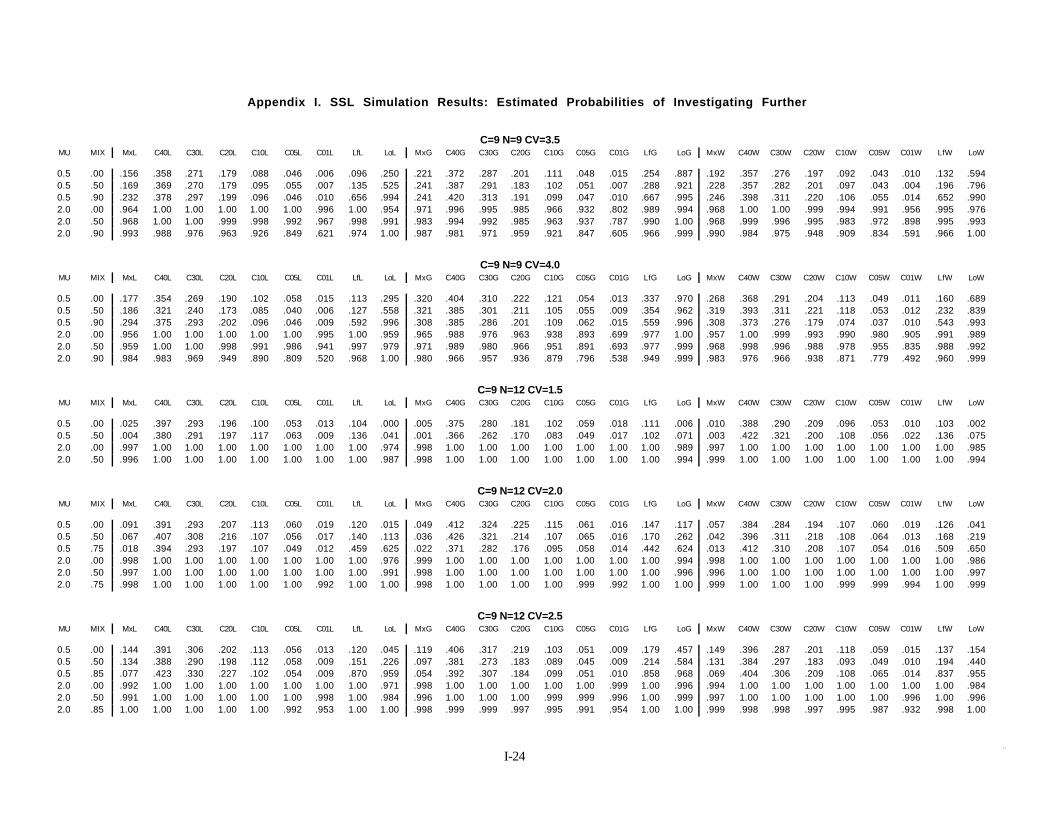
I-242 4
Appendix I. SSL Simulation Results: Estimated Probabilities of Investigating Further
C=9 N=9 CV=3.5MU MIX MxL C40L C30L C20L C10L C05L C01L LfL LoL MxG C40G C30G C20G C10G C05G C01G LfG LoG MxW C40W C30W C20W C10W C05W C01W LfW LoW
0.5 .00 .156 .358 .271 .179 .088 .046 .006 .096 .250 .221 .372 .287 .201 .111 .048 .015 .254 .887 .192 .357 .276 .197 .092 .043 .010 .132 .5940.5 .50 .169 .369 .270 .179 .095 .055 .007 .135 .525 .241 .387 .291 .183 .102 .051 .007 .288 .921 .228 .357 .282 .201 .097 .043 .004 .196 .7960.5 .90 .232 .378 .297 .199 .096 .046 .010 .656 .994 .241 .420 .313 .191 .099 .047 .010 .667 .995 .246 .398 .311 .220 .106 .055 .014 .652 .9902.0 .00 .964 1.00 1.00 1.00 1.00 1.00 .996 1.00 .954 .971 .996 .995 .985 .966 .932 .802 .989 .994 .968 1.00 1.00 .999 .994 .991 .956 .995 .9762.0 .50 .968 1.00 1.00 .999 .998 .992 .967 .998 .991 .983 .994 .992 .985 .963 .937 .787 .990 1.00 .968 .999 .996 .995 .983 .972 .898 .995 .9932.0 .90 .993 .988 .976 .963 .926 .849 .621 .974 1.00 .987 .981 .971 .959 .921 .847 .605 .966 .999 .990 .984 .975 .948 .909 .834 .591 .966 1.00
C=9 N=9 CV=4.0MU MIX MxL C40L C30L C20L C10L C05L C01L LfL LoL MxG C40G C30G C20G C10G C05G C01G LfG LoG MxW C40W C30W C20W C10W C05W C01W LfW LoW
0.5 .00 .177 .354 .269 .190 .102 .058 .015 .113 .295 .320 .404 .310 .222 .121 .054 .013 .337 .970 .268 .368 .291 .204 .113 .049 .011 .160 .6890.5 .50 .186 .321 .240 .173 .085 .040 .006 .127 .558 .321 .385 .301 .211 .105 .055 .009 .354 .962 .319 .393 .311 .221 .118 .053 .012 .232 .8390.5 .90 .294 .375 .293 .202 .096 .046 .009 .592 .996 .308 .385 .286 .201 .109 .062 .015 .559 .996 .308 .373 .276 .179 .074 .037 .010 .543 .9932.0 .00 .956 1.00 1.00 1.00 1.00 1.00 .995 1.00 .959 .965 .988 .976 .963 .938 .893 .699 .977 1.00 .957 1.00 .999 .993 .990 .980 .905 .991 .9892.0 .50 .959 1.00 1.00 .998 .991 .986 .941 .997 .979 .971 .989 .980 .966 .951 .891 .693 .977 .999 .968 .998 .996 .988 .978 .955 .835 .988 .9922.0 .90 .984 .983 .969 .949 .890 .809 .520 .968 1.00 .980 .966 .957 .936 .879 .796 .538 .949 .999 .983 .976 .966 .938 .871 .779 .492 .960 .999
C=9 N=12 CV=1.5MU MIX MxL C40L C30L C20L C10L C05L C01L LfL LoL MxG C40G C30G C20G C10G C05G C01G LfG LoG MxW C40W C30W C20W C10W C05W C01W LfW LoW
0.5 .00 .025 .397 .293 .196 .100 .053 .013 .104 .000 .005 .375 .280 .181 .102 .059 .018 .111 .006 .010 .388 .290 .209 .096 .053 .010 .103 .0020.5 .50 .004 .380 .291 .197 .117 .063 .009 .136 .041 .001 .366 .262 .170 .083 .049 .017 .102 .071 .003 .422 .321 .200 .108 .056 .022 .136 .0752.0 .00 .997 1.00 1.00 1.00 1.00 1.00 1.00 1.00 .974 .998 1.00 1.00 1.00 1.00 1.00 1.00 1.00 .989 .997 1.00 1.00 1.00 1.00 1.00 1.00 1.00 .9852.0 .50 .996 1.00 1.00 1.00 1.00 1.00 1.00 1.00 .987 .998 1.00 1.00 1.00 1.00 1.00 1.00 1.00 .994 .999 1.00 1.00 1.00 1.00 1.00 1.00 1.00 .994
C=9 N=12 CV=2.0MU MIX MxL C40L C30L C20L C10L C05L C01L LfL LoL MxG C40G C30G C20G C10G C05G C01G LfG LoG MxW C40W C30W C20W C10W C05W C01W LfW LoW
0.5 .00 .091 .391 .293 .207 .113 .060 .019 .120 .015 .049 .412 .324 .225 .115 .061 .016 .147 .117 .057 .384 .284 .194 .107 .060 .019 .126 .0410.5 .50 .067 .407 .308 .216 .107 .056 .017 .140 .113 .036 .426 .321 .214 .107 .065 .016 .170 .262 .042 .396 .311 .218 .108 .064 .013 .168 .2190.5 .75 .018 .394 .293 .197 .107 .049 .012 .459 .625 .022 .371 .282 .176 .095 .058 .014 .442 .624 .013 .412 .310 .208 .107 .054 .016 .509 .6502.0 .00 .998 1.00 1.00 1.00 1.00 1.00 1.00 1.00 .976 .999 1.00 1.00 1.00 1.00 1.00 1.00 1.00 .994 .998 1.00 1.00 1.00 1.00 1.00 1.00 1.00 .9862.0 .50 .997 1.00 1.00 1.00 1.00 1.00 1.00 1.00 .991 .998 1.00 1.00 1.00 1.00 1.00 1.00 1.00 .996 .996 1.00 1.00 1.00 1.00 1.00 1.00 1.00 .9972.0 .75 .998 1.00 1.00 1.00 1.00 1.00 .992 1.00 1.00 .998 1.00 1.00 1.00 1.00 .999 .992 1.00 1.00 .999 1.00 1.00 1.00 .999 .999 .994 1.00 .999
C=9 N=12 CV=2.5MU MIX MxL C40L C30L C20L C10L C05L C01L LfL LoL MxG C40G C30G C20G C10G C05G C01G LfG LoG MxW C40W C30W C20W C10W C05W C01W LfW LoW
0.5 .00 .144 .391 .306 .202 .113 .056 .013 .120 .045 .119 .406 .317 .219 .103 .051 .009 .179 .457 .149 .396 .287 .201 .118 .059 .015 .137 .1540.5 .50 .134 .388 .290 .198 .112 .058 .009 .151 .226 .097 .381 .273 .183 .089 .045 .009 .214 .584 .131 .384 .297 .183 .093 .049 .010 .194 .4400.5 .85 .077 .423 .330 .227 .102 .054 .009 .870 .959 .054 .392 .307 .184 .099 .051 .010 .858 .968 .069 .404 .306 .209 .108 .065 .014 .837 .9552.0 .00 .992 1.00 1.00 1.00 1.00 1.00 1.00 1.00 .971 .998 1.00 1.00 1.00 1.00 1.00 .999 1.00 .996 .994 1.00 1.00 1.00 1.00 1.00 1.00 1.00 .9842.0 .50 .991 1.00 1.00 1.00 1.00 1.00 .998 1.00 .984 .996 1.00 1.00 1.00 .999 .999 .996 1.00 .999 .997 1.00 1.00 1.00 1.00 1.00 .996 1.00 .9962.0 .85 1.00 1.00 1.00 1.00 1.00 .992 .953 1.00 1.00 .998 .999 .999 .997 .995 .991 .954 1.00 1.00 .999 .998 .998 .997 .995 .987 .932 .998 1.00

I-252 5
Appendix I. SSL Simulation Results: Estimated Probabilities of Investigating Further
C=9 N=12 CV=3.0MU MIX MxL C40L C30L C20L C10L C05L C01L LfL LoL MxG C40G C30G C20G C10G C05G C01G LfG LoG MxW C40W C30W C20W C10W C05W C01W LfW LoW
0.5 .00 .150 .356 .260 .184 .089 .038 .007 .101 .073 .234 .406 .318 .211 .117 .055 .015 .268 .745 .222 .385 .302 .205 .107 .048 .012 .145 .3490.5 .50 .176 .350 .264 .160 .087 .050 .009 .127 .297 .233 .405 .309 .223 .123 .057 .012 .309 .822 .237 .382 .305 .208 .098 .053 .014 .209 .6240.5 .85 .174 .413 .317 .220 .123 .068 .012 .752 .977 .188 .400 .299 .206 .111 .056 .010 .728 .974 .180 .406 .296 .192 .094 .051 .010 .730 .9802.0 .00 .996 1.00 1.00 1.00 1.00 1.00 1.00 1.00 .968 .995 1.00 1.00 1.00 1.00 .998 .971 1.00 .997 .992 1.00 1.00 1.00 1.00 1.00 .998 1.00 .9892.0 .50 .992 1.00 1.00 1.00 1.00 1.00 .999 1.00 .989 .998 .999 .999 .999 .997 .993 .967 .999 .999 .996 1.00 1.00 .999 .998 .995 .981 1.00 .9982.0 .85 .999 1.00 .998 .995 .983 .976 .908 .999 1.00 .995 .995 .995 .995 .989 .980 .905 .996 1.00 .998 1.00 .999 .996 .991 .976 .898 1.00 1.00
C=9 N=12 CV=3.5MU MIX MxL C40L C30L C20L C10L C05L C01L LfL LoL MxG C40G C30G C20G C10G C05G C01G LfG LoG MxW C40W C30W C20W C10W C05W C01W LfW LoW
0.5 .00 .215 .378 .308 .208 .105 .047 .010 .122 .152 .338 .384 .308 .207 .102 .054 .008 .342 .892 .288 .383 .284 .197 .089 .043 .009 .144 .4490.5 .50 .237 .372 .288 .201 .097 .048 .011 .160 .400 .303 .378 .293 .175 .090 .047 .006 .359 .921 .305 .388 .310 .224 .106 .057 .012 .242 .7380.5 .90 .293 .392 .303 .202 .109 .058 .010 .772 .997 .289 .397 .309 .203 .094 .034 .009 .753 .998 .317 .409 .300 .207 .113 .066 .015 .744 1.002.0 .00 .988 1.00 1.00 1.00 1.00 1.00 .998 1.00 .953 .990 1.00 .999 .993 .986 .980 .917 .996 .999 .994 1.00 1.00 1.00 .999 .998 .993 1.00 .9882.0 .50 .990 1.00 1.00 1.00 1.00 .999 .991 1.00 .990 .995 .999 .999 .996 .987 .976 .895 .995 .998 .989 1.00 .999 .999 .998 .995 .962 .998 .9942.0 .90 .998 .989 .986 .979 .962 .933 .787 .984 1.00 .998 .994 .989 .983 .958 .921 .766 .988 1.00 .999 .997 .993 .987 .960 .931 .772 .994 1.00
C=9 N=12 CV=4.0MU MIX MxL C40L C30L C20L C10L C05L C01L LfL LoL MxG C40G C30G C20G C10G C05G C01G LfG LoG MxW C40W C30W C20W C10W C05W C01W LfW LoW
0.5 .00 .225 .334 .261 .180 .087 .036 .004 .097 .149 .410 .397 .323 .219 .112 .059 .012 .374 .949 .309 .359 .262 .171 .084 .043 .005 .139 .5550.5 .50 .279 .368 .286 .208 .107 .050 .006 .153 .476 .372 .371 .273 .195 .092 .041 .013 .379 .967 .360 .383 .288 .192 .103 .045 .007 .255 .8210.5 .90 .389 .401 .294 .214 .111 .063 .017 .687 .997 .428 .412 .323 .212 .101 .058 .011 .664 .999 .429 .415 .312 .217 .116 .057 .012 .678 .9982.0 .00 .987 1.00 1.00 1.00 1.00 1.00 .999 1.00 .961 .992 .997 .992 .990 .970 .944 .841 .994 1.00 .990 1.00 .999 .999 .999 .998 .972 .999 .9942.0 .50 .992 1.00 1.00 1.00 1.00 .999 .994 1.00 .986 .990 .991 .990 .988 .972 .948 .832 .992 1.00 .992 .999 .998 .996 .995 .988 .920 .997 .9962.0 .90 .997 .993 .986 .977 .953 .903 .746 .987 1.00 1.00 .996 .990 .980 .955 .907 .712 .991 1.00 .994 .989 .981 .971 .940 .892 .720 .986 1.00
C=9 N=16 CV=1.5MU MIX MxL C40L C30L C20L C10L C05L C01L LfL LoL MxG C40G C30G C20G C10G C05G C01G LfG LoG MxW C40W C30W C20W C10W C05W C01W LfW LoW
0.5 .00 .052 .412 .318 .213 .100 .052 .010 .110 .000 .004 .390 .313 .205 .099 .053 .008 .117 .000 .020 .415 .306 .212 .110 .050 .009 .131 .0000.5 .50 .010 .388 .286 .181 .102 .058 .014 .139 .038 .005 .378 .288 .193 .091 .042 .011 .146 .051 .009 .397 .304 .200 .108 .055 .015 .148 .0402.0 .00 1.00 1.00 1.00 1.00 1.00 1.00 1.00 1.00 .978 .999 1.00 1.00 1.00 1.00 1.00 1.00 1.00 .990 .999 1.00 1.00 1.00 1.00 1.00 1.00 1.00 .9862.0 .50 1.00 1.00 1.00 1.00 1.00 1.00 1.00 1.00 .991 1.00 1.00 1.00 1.00 1.00 1.00 1.00 1.00 .988 1.00 1.00 1.00 1.00 1.00 1.00 1.00 1.00 .997
C=9 N=16 CV=2.0MU MIX MxL C40L C30L C20L C10L C05L C01L LfL LoL MxG C40G C30G C20G C10G C05G C01G LfG LoG MxW C40W C30W C20W C10W C05W C01W LfW LoW
0.5 .00 .091 .372 .283 .198 .103 .058 .014 .110 .002 .070 .393 .306 .191 .096 .043 .012 .137 .050 .064 .363 .263 .186 .091 .046 .008 .121 .0050.5 .50 .077 .372 .287 .197 .111 .062 .019 .145 .059 .048 .374 .286 .187 .104 .065 .016 .204 .191 .058 .396 .311 .216 .103 .056 .015 .200 .1560.5 .75 .020 .373 .295 .197 .105 .058 .014 .566 .701 .023 .394 .300 .208 .096 .047 .010 .567 .702 .023 .398 .311 .213 .114 .066 .020 .614 .7352.0 .00 1.00 1.00 1.00 1.00 1.00 1.00 1.00 1.00 .976 1.00 1.00 1.00 1.00 1.00 1.00 1.00 1.00 .998 1.00 1.00 1.00 1.00 1.00 1.00 1.00 1.00 .9852.0 .50 1.00 1.00 1.00 1.00 1.00 1.00 1.00 1.00 .989 .999 1.00 1.00 1.00 1.00 1.00 1.00 1.00 .997 1.00 1.00 1.00 1.00 1.00 1.00 1.00 1.00 .9992.0 .75 1.00 1.00 1.00 1.00 1.00 1.00 1.00 1.00 1.00 1.00 1.00 1.00 1.00 1.00 1.00 .999 1.00 1.00 1.00 1.00 1.00 1.00 1.00 1.00 .998 1.00 1.00

I-262 6
Appendix I. SSL Simulation Results: Estimated Probabilities of Investigating Further
C=9 N=16 CV=2.5MU MIX MxL C40L C30L C20L C10L C05L C01L LfL LoL MxG C40G C30G C20G C10G C05G C01G LfG LoG MxW C40W C30W C20W C10W C05W C01W LfW LoW
0.5 .00 .163 .379 .281 .198 .113 .052 .008 .124 .012 .170 .397 .297 .199 .098 .054 .009 .216 .331 .170 .380 .279 .186 .103 .053 .013 .140 .0660.5 .50 .187 .396 .306 .209 .113 .056 .019 .158 .121 .145 .388 .282 .190 .090 .048 .013 .269 .467 .161 .404 .301 .208 .105 .051 .008 .226 .3300.5 .85 .071 .420 .322 .207 .098 .053 .014 .952 .984 .065 .438 .331 .232 .107 .062 .015 .963 .986 .085 .406 .304 .201 .106 .058 .018 .942 .9882.0 .00 .998 1.00 1.00 1.00 1.00 1.00 1.00 1.00 .966 .998 1.00 1.00 1.00 1.00 1.00 1.00 1.00 .996 .998 1.00 1.00 1.00 1.00 1.00 1.00 1.00 .9862.0 .50 1.00 1.00 1.00 1.00 1.00 1.00 1.00 1.00 .995 1.00 1.00 1.00 1.00 1.00 1.00 .999 1.00 1.00 .999 1.00 1.00 1.00 1.00 1.00 1.00 1.00 .9962.0 .85 1.00 1.00 1.00 1.00 .998 .997 .982 1.00 1.00 1.00 1.00 1.00 1.00 1.00 .998 .989 1.00 1.00 1.00 1.00 1.00 1.00 1.00 .997 .983 1.00 1.00
C=9 N=16 CV=3.0MU MIX MxL C40L C30L C20L C10L C05L C01L LfL LoL MxG C40G C30G C20G C10G C05G C01G LfG LoG MxW C40W C30W C20W C10W C05W C01W LfW LoW
0.5 .00 .227 .400 .315 .210 .105 .053 .005 .125 .026 .279 .366 .269 .192 .099 .047 .007 .287 .655 .278 .383 .292 .205 .106 .057 .013 .170 .1740.5 .50 .256 .390 .302 .224 .124 .049 .011 .184 .207 .297 .376 .291 .204 .104 .047 .007 .361 .766 .286 .399 .299 .192 .097 .060 .017 .271 .5480.5 .85 .252 .387 .277 .186 .093 .050 .011 .860 .982 .225 .368 .282 .186 .093 .045 .011 .829 .991 .247 .430 .336 .229 .135 .074 .015 .851 .9872.0 .00 .998 1.00 1.00 1.00 1.00 1.00 1.00 1.00 .961 .999 1.00 1.00 1.00 .999 .998 .997 .999 .997 .999 1.00 1.00 1.00 1.00 1.00 1.00 1.00 .9892.0 .50 1.00 1.00 1.00 1.00 1.00 1.00 1.00 1.00 .993 .999 1.00 1.00 1.00 1.00 1.00 .991 1.00 1.00 1.00 1.00 1.00 1.00 1.00 1.00 1.00 1.00 1.002.0 .85 1.00 1.00 1.00 .999 .997 .991 .971 1.00 1.00 1.00 1.00 1.00 1.00 .998 .993 .964 1.00 1.00 1.00 1.00 1.00 1.00 .996 .995 .968 1.00 1.00
C=9 N=16 CV=3.5MU MIX MxL C40L C30L C20L C10L C05L C01L LfL LoL MxG C40G C30G C20G C10G C05G C01G LfG LoG MxW C40W C30W C20W C10W C05W C01W LfW LoW
0.5 .00 .271 .365 .283 .202 .114 .071 .009 .130 .070 .392 .368 .276 .180 .085 .041 .010 .387 .867 .348 .374 .294 .201 .103 .056 .014 .166 .2910.5 .50 .319 .353 .278 .190 .098 .058 .009 .162 .271 .382 .366 .282 .199 .097 .050 .013 .441 .918 .397 .419 .319 .220 .113 .052 .011 .295 .6780.5 .90 .396 .432 .338 .224 .118 .058 .015 .846 1.00 .351 .387 .289 .198 .106 .044 .010 .822 1.00 .351 .411 .325 .223 .113 .061 .006 .843 1.002.0 .00 .995 1.00 1.00 1.00 1.00 1.00 1.00 1.00 .961 .999 1.00 1.00 1.00 1.00 .998 .976 1.00 1.00 .999 1.00 1.00 1.00 1.00 1.00 .999 1.00 .9912.0 .50 .999 1.00 1.00 1.00 1.00 1.00 .999 1.00 .991 .998 1.00 1.00 1.00 .999 .993 .968 1.00 1.00 1.00 1.00 1.00 1.00 .999 .999 .994 .999 1.002.0 .90 1.00 .997 .996 .993 .985 .970 .902 .995 1.00 1.00 .999 .997 .997 .991 .975 .887 .999 1.00 1.00 .998 .996 .993 .980 .970 .881 .996 1.00
C=9 N=16 CV=4.0MU MIX MxL C40L C30L C20L C10L C05L C01L LfL LoL MxG C40G C30G C20G C10G C05G C01G LfG LoG MxW C40W C30W C20W C10W C05W C01W LfW LoW
0.5 .00 .297 .353 .276 .202 .111 .052 .014 .125 .072 .502 .379 .282 .176 .088 .049 .010 .438 .949 .414 .358 .280 .183 .090 .039 .005 .165 .3940.5 .50 .379 .393 .305 .209 .102 .053 .004 .181 .337 .513 .413 .325 .215 .116 .066 .015 .513 .967 .441 .377 .288 .207 .095 .046 .010 .293 .7790.5 .90 .481 .402 .294 .198 .100 .049 .011 .793 1.00 .493 .387 .298 .201 .091 .047 .011 .738 .999 .493 .389 .315 .196 .102 .053 .010 .773 1.002.0 .00 .998 1.00 1.00 1.00 1.00 1.00 .999 1.00 .950 .996 .998 .998 .995 .991 .981 .932 .997 1.00 .998 1.00 1.00 1.00 1.00 1.00 .996 1.00 .9942.0 .50 .997 1.00 1.00 1.00 1.00 1.00 .998 1.00 .990 .999 .998 .998 .995 .991 .982 .923 1.00 1.00 .997 1.00 1.00 1.00 .999 .997 .979 1.00 .9992.0 .90 1.00 1.00 .997 .991 .979 .952 .872 .998 1.00 .999 .998 .995 .992 .970 .934 .817 .994 1.00 1.00 .998 .995 .986 .973 .939 .820 .994 1.00

APPENDIX J
Piazza Road Simulation Results

APPENDIX J
Piazza Road Simulation Results
Section 4.3.6 contains background information on the Piazza Road site and its seven exposure areas(EAs), as well as a complete description of the simulation setup and parameters. The followingnotation is used in the tables of this appendix.
EA = exposure area number (from 1 to 7)
MEAN = the true mean for the EA (an average of 96 measurements)
CV = the true value of the coefficient of variation for the EA
DES = indicator of whether compositing within strata (DES = W) or compositingacross strata (DES = X) was used
C = the number of specimens per composite
N = the number of composite samples chemically analyzed.
The remaining four variables give the estimated error rates at 0.5 SSL and 2 SSL for the Max test(labelled as MAX 0.5SSL and MAX 2.0SSL) and the Chen test at the nominal .10 level (labelled asCHEN 0.5SSL and CHEN 2.0SSL).
J-1

Appendix J. Estimated decision error rates for Chen test at the 0.1 level, and Max test, forcompositing within sector (DES=W) or across sector (DES=X), based on simulations from PiazzaRoad Data.
EA = EA # (1 to 7). MEAN and CV denote EA true mean and CV.M = # of samples per composite. N = # of composite samples.
-------------------------- EA=1 MEAN=2.1 CV=1.0 --------------------------
DES M NMAX
0.5SSLMAX
2.0SSLCHEN
0.5SSLCHEN
2.0SSL
W 4 4 .01 .03 .02 .00
X 4 4 .00 .12 .12 .00
W 4 6 .01 .01 .04 .00
X 4 6 .00 .04 .11 .00
W 4 8 .02 .00 .01 .00
X 4 8 .00 .01 .15 .00
W 6 4 .00 .01 .01 .00
X 6 4 .00 .11 .13 .00
W 6 6 .00 .01 .04 .00
X 6 6 .00 .04 .12 .00
W 6 8 .01 .00 .01 .00
X 6 8 .00 .01 .12 .00
W 8 4 .00 .02 .00 .00
X 8 4 .00 .09 .12 .00
W 8 6 .00 .01 .02 .00
X 8 6 .00 .04 .13 .00
W 8 8 .00 .00 .01 .00
X 8 8 .00 .02 .10 .00
-------------------------- EA=2 MEAN=2.4 CV=1.6 --------------------------
DES M NMAX
0.5SSLMAX
2.0SSLCHEN
0.5SSLCHEN
2.0SSL
W 4 4 .07 .13 .08 .05
X 4 4 .04 .13 .11 .05
W 4 6 .09 .04 .05 .02
X 4 6 .05 .05 .11 .01
W 4 8 .11 .02 .05 .00
X 4 8 .07 .01 .11 .00
W 6 4 .04 .13 .09 .02
X 6 4 .01 .14 .09 .02
W 6 6 .05 .03 .04 .00
X 6 6 .01 .04 .09 .00
W 6 8 .06 .01 .04 .00
X 6 8 .01 .01 .13 .00
W 8 4 .03 .08 .09 .00
X 8 4 .00 .12 .10 .01
W 8 6 .04 .02 .04 .00
X 8 6 .00 .04 .10 .00
W 8 8 .04 .00 .04 .00
X 8 8 .00 .02 .12 .00
J-2

Appendix J. Estimated decision error rates for Chen test at the 0.1 level, and Max test, forcompositing within sector (DES=W) or across sector (DES=X), based on simulations from PiazzaRoad Data.
EA = EA # (1 to 7). MEAN and CV denote EA true mean and CV.M = # of samples per composite. N = # of composite samples.
-----------------------------EA=3 MEAN=5.1 CV=1.1-----------------------------
DES M NMAX
0.5SSLMAX
2.0SSLCHEN
0.5SSLCHEN
2.0SSL
W 4 4 .01 .03 .03 .01
X 4 4 .00 .11 .14 .00
W 4 6 .02 .00 .00 .00
X 4 6 .00 .03 .11 .00
W 4 8 .06 .00 .00 .00
X 4 8 .00 .01 .10 .00
W 6 4 .00 .02 .01 .00
X 6 4 .00 .09 .12 .00
W 6 6 .01 .00 .00 .00
X 6 6 .00 .03 .11 .00
W 6 8 .02 .00 .00 .00
X 6 8 .00 .01 .11 .00
W 8 4 .00 .02 .01 .00
X 8 4 .00 .10 .14 .00
W 8 6 .01 .00 .00 .00
X 8 6 .00 .03 .12 .00
W 8 8 .03 .00 .00 .00
X 8 8 .00 .01 .12 .00
-----------------------------EA=4 MEAN=3.8 CV=1.2-----------------------------
DES M NMAX
0.5SSLMAX
2.0SSLCHEN
0.5SSLCHEN
2.0SSL
W 4 4 .01 .11 .07 .00
X 4 4 .00 .11 .10 .00
W 4 6 .02 .04 .06 .00
X 4 6 .00 .04 .11 .00
W 4 8 .02 .01 .05 .00
X 4 8 .00 .01 .09 .00
W 6 4 .01 .10 .05 .00
X 6 4 .00 .10 .12 .00
W 6 6 .00 .02 .04 .00
X 6 6 .00 .03 .09 .00
W 6 8 .01 .01 .04 .00
X 6 8 .00 .02 .10 .00
W 8 4 .00 .09 .04 .00
X 8 4 .00 .12 .12 .00
W 8 6 .00 .03 .06 .00
X 8 6 .00 .03 .11 .00
W 8 8 .00 .01 .03 .00
X 8 8 .00 .01 .11 .00
J-3

Appendix J. Estimated decision error rates for Chen test at the 0.1 level, and Max test, forcompositing within sector (DES=W) or across sector (DES=X), based on simulations from PiazzaRoad Data.
EA = EA # (1 to 7). MEAN and CV denote EA true mean and CV.M = # of samples per composite. N = # of composite samples.
-----------------------------EA=5 MEAN=9.3 CV=2.0-----------------------------
DES M NMAX
0.5SSLMAX
2.0SSLCHEN
0.5SSLCHEN
2.0SSL
W 4 4 .22 .13 .01 .12
X 4 4 .03 .17 .07 .04
W 4 6 .48 .03 .00 .02
X 4 6 .03 .06 .08 .00
W 4 8 .71 .00 .00 .00
X 4 8 .05 .03 .10 .00
W 6 4 .18 .06 .00 .05
X 6 4 .00 .10 .10 .01
W 6 6 .47 .01 .00 .00
X 6 6 .00 .02 .10 .00
W 6 8 .76 .00 .00 .00
X 6 8 .00 .01 .11 .00
W 8 4 .19 .05 .00 .03
X 8 4 .00 .08 .12 .00
W 8 6 .45 .01 .00 .00
X 8 6 .00 .03 .14 .00
W 8 8 .76 .00 .00 .00
X 8 8 .00 .01 .10 .00
----------------------------EA=6 MEAN=15.8 CV=2.2-----------------------------
DES M NMAX
0.5SSLMAX
2.0SSLCHEN
0.5SSLCHEN
2.0SSL
W 4 4 .18 .16 .03 .21
X 4 4 .07 .20 .10 .19
W 4 6 .22 .06 .03 .07
X 4 6 .10 .08 .09 .07
W 4 8 .34 .03 .02 .03
X 4 8 .13 .03 .09 .03
W 6 4 .13 .11 .02 .11
X 6 4 .02 .16 .09 .09
W 6 6 .15 .04 .02 .03
X 6 6 .05 .06 .08 .02
W 6 8 .33 .01 .02 .01
X 6 8 .07 .03 .09 .01
W 8 4 .08 .09 .00 .07
X 8 4 .01 .14 .09 .03
W 8 6 .11 .03 .01 .01
X 8 6 .01 .04 .09 .01
W 8 8 .31 .01 .01 .00
X 8 8 .01 .02 .10 .00
J-4

Appendix J. Estimated decision error rates for Chen test at the 0.1 level, and Max test, forcompositing within sector (DES=W) or across sector (DES=X), based on simulations from PiazzaRoad Data.
EA = EA # (1 to 7). MEAN and CV denote EA true mean and CV.M = # of samples per composite. N = # of composite samples.
-----------------------------EA=7 MEAN=2.8 CV=1.4-----------------------------
DES M NMAX
0.5SSLMAX
2.0SSLCHEN
0.5SSLCHEN
2.0SSL
W 4 4 .03 .11 .02 .00
X 4 4 .00 .13 .09 .00
W 4 6 .09 .03 .02 .00
X 4 6 .01 .06 .07 .00
W 4 8 .16 .01 .02 .00
X 4 8 .01 .02 .09 .00
W 6 4 .02 .08 .01 .00
X 6 4 .00 .10 .12 .00
W 6 6 .06 .02 .01 .00
X 6 6 .00 .03 .09 .00
W 6 8 .10 .00 .01 .00
X 6 8 .00 .02 .09 .00
W 8 4 .01 .06 .01 .00
X 8 4 .00 .10 .12 .00
W 8 6 .04 .01 .00 .00
X 8 6 .00 .03 .10 .00
W 8 8 .06 .00 .00 .00
X 8 8 .00 .01 .11 .00
J-5

APPENDIX K
Soil Organic Carbon (Koc) / Water (Kow) PartitionCoefficients
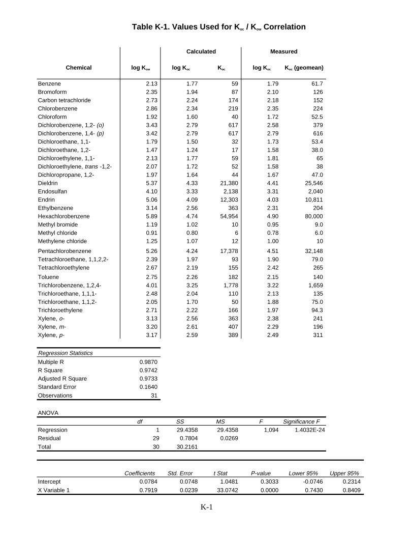
Table K-1. Values Used for Koc / Kow Correlation
Calculated Measured
Chemical log Kow log Koc Koc log Koc Koc (geomean)
Benzene 2.13 1.77 59 1.79 61.7Bromoform 2.35 1.94 87 2.10 126Carbon tetrachloride 2.73 2.24 174 2.18 152Chlorobenzene 2.86 2.34 219 2.35 224Chloroform 1.92 1.60 40 1.72 52.5Dichlorobenzene, 1,2- (o) 3.43 2.79 617 2.58 379Dichlorobenzene, 1,4- (p) 3.42 2.79 617 2.79 616Dichloroethane, 1,1- 1.79 1.50 32 1.73 53.4Dichloroethane, 1,2- 1.47 1.24 17 1.58 38.0Dichloroethylene, 1,1- 2.13 1.77 59 1.81 65Dichloroethylene, trans -1,2- 2.07 1.72 52 1.58 38Dichloropropane, 1,2- 1.97 1.64 44 1.67 47.0Dieldrin 5.37 4.33 21,380 4.41 25,546Endosulfan 4.10 3.33 2,138 3.31 2,040Endrin 5.06 4.09 12,303 4.03 10,811Ethylbenzene 3.14 2.56 363 2.31 204Hexachlorobenzene 5.89 4.74 54,954 4.90 80,000Methyl bromide 1.19 1.02 10 0.95 9.0Methyl chloride 0.91 0.80 6 0.78 6.0Methylene chloride 1.25 1.07 12 1.00 10
Pentachlorobenzene 5.26 4.24 17,378 4.51 32,148Tetrachloroethane, 1,1,2,2- 2.39 1.97 93 1.90 79.0Tetrachloroethylene 2.67 2.19 155 2.42 265
Toluene 2.75 2.26 182 2.15 140Trichlorobenzene, 1,2,4- 4.01 3.25 1,778 3.22 1,659Trichloroethane, 1,1,1- 2.48 2.04 110 2.13 135Trichloroethane, 1,1,2- 2.05 1.70 50 1.88 75.0Trichloroethylene 2.71 2.22 166 1.97 94.3Xylene, o- 3.13 2.56 363 2.38 241Xylene, m- 3.20 2.61 407 2.29 196Xylene, p- 3.17 2.59 389 2.49 311
Regression Statistics
Multiple R 0.9870R Square 0.9742Adjusted R Square 0.9733Standard Error 0.1640
Observations 31
ANOVA
df SS MS F Significance FRegression 1 29.4358 29.4358 1,094 1.4032E-24Residual 29 0.7804 0.0269
Total 30 30.2161
Coefficients Std. Error t Stat P-value Lower 95% Upper 95%Intercept 0.0784 0.0748 1.0481 0.3033 -0.0746 0.2314
X Variable 1 0.7919 0.0239 33.0742 0.0000 0.7430 0.8409
K-1
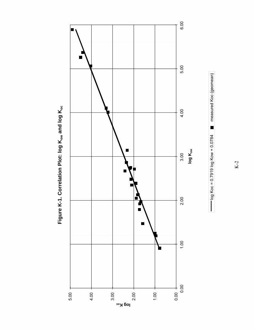
K-2
Fig
ure
K-1
. Co
rrel
atio
n P
lot:
log
Ko
w a
nd
log
Ko
c
0.00
1.00
2.00
3.00
4.00
5.00
0.00
1.00
2.00
3.00
4.00
5.00
6.00
log
Ko
w
log Koc
log
Koc
= 0
.791
9 lo
g K
ow +
0.0
784
mea
sure
d K
oc (
geom
ean)

Tab
le K
-2. C
olle
cted
Ko
c Val
ues
(H
ydro
ph
ob
ic O
rgan
ics)
Ch
emic
alC
AS
No
.K
oc
(L/k
g)
Lo
g K
oc
So
urc
eC
om
men
ts
Ace
nap
hth
ene
83-3
2-9
3,89
03.
59S
zabo
(19
90a)
RP
-HP
LC o
n P
IHA
C (
hum
ic a
cids
)
6,16
63.
79S
zabo
(19
90a)
RP
-HP
LC o
n C
IHA
C (
hum
ic a
cids
)
Ave
rag
e5,
028
3.70
Geo
met
ric
Mea
n4,
898
3.69
Ace
ton
e67
-64-
1
Ald
rin
309-
00-2
48,3
944.
68Lo
rd e
t al.
(198
0)"G
eesc
roft/
Rot
ham
sted
Far
m"
soil;
2.6
% O
M; p
H=
5.1;
sus
pect
48,9
784.
69B
riggs
(19
81)
Bat
com
be s
ilt lo
am (
Gr.
Br.
); 2
.05%
OC
; pH
=6.
1
Ave
rag
e48
,686
4.69
Geo
met
ric
Mea
n48
,685
4.69
An
thra
cen
e12
0-12
-7
14,5
004.
16M
cCar
thy
& J
imen
ez (
1985
)hu
mic
aci
ds
15,8
494.
20K
aric
hkof
f (19
81)
soil/
sedi
men
ts a
vera
ge; s
hake
-fla
sk U
V
19,5
624.
29La
ndru
m e
t al.
(198
4)su
rfac
e w
ater
(ge
omea
n 5
valu
es)
23,9
884.
38H
odso
n &
Will
iam
s (1
988)
cyan
opro
pyl c
olum
n; H
PLC
26,0
004.
41K
aric
khof
f et a
l. (1
979)
avg.
coa
rse
silt
frac
tion,
Doe
Run
& H
icko
ry H
ill s
edim
ents
26,3
034.
42S
zabo
et a
l. (1
990a
)R
P-H
PLC
on
PIH
AC
(hu
mic
aci
ds)
27,8
404.
44A
bdul
& G
ibso
n (1
986)
Flin
t aqu
ifer
sam
ple;
87%
san
d; fo
c =
0.0
187
31,3
294.
50La
ndru
m e
t al.
(198
4)hu
mic
aci
d (g
eom
ean
8 va
lues
)
33,8
844.
53S
zabo
et a
l. (1
990a
)R
P-H
PLC
on
CIH
AC
(hu
mic
aci
ds)
Ave
rag
e24
,362
4.39
Geo
met
ric
Mea
n23
,493
4.37
Ben
z(α)
anth
race
ne
56-5
5-3
150,
000
5.18
McC
arth
y &
Jim
enez
(19
85)
hum
ic a
cid
199,
526
5.30
Land
rum
et a
l. (1
984)
hum
ic a
cid
650,
000
5.81
Kar
ickh
off e
t al.
(197
9)av
g. c
oars
e si
lt fr
actio
n, D
oe R
un &
Hic
kory
Hill
sed
s.
840,
000
5.92
Sm
ith e
t al.
(197
8) a
s ci
ted
in D
i Tor
o et
al.
(198
5)40
% O
C
Ave
rag
e45
9,88
25.
66
Geo
met
ric
Mea
n35
7,53
75.
55
Ben
zen
e71
-43-
2
311.
50C
hiou
et a
l. (1
983)
Woo
dbur
n si
lt lo
am; f
om =
0.0
19; 2
1% c
lay
38.2
1.58
Sei
p et
al.
(198
6)fo
rest
soi
l with
0.2
% O
C; c
olum
n st
udy
43.5
1.64
Sei
p et
al.
(198
6)ag
ricul
tura
l soi
l with
2.2
% O
C; c
olum
n st
udy
491.
69A
bdul
et a
l. (1
987)
batc
h eq
uilib
rium
exp
erim
ents
; aqu
ifer
mat
eria
l; fo
c =
0.0
105
53.5
1.73
Sei
p et
al.
(198
6)fo
rest
soi
l with
3.7
% O
C; c
olum
n st
udy
601.
78K
aric
khof
f (19
81)
soils
/sed
imen
ts a
vera
ge; s
hake
flas
k U
V
K-3

Tab
le K
-2. C
olle
cted
Ko
c Val
ues
(H
ydro
ph
ob
ic O
rgan
ics)
Ch
emic
alC
AS
No
.K
oc
(L/k
g)
Lo
g K
oc
So
urc
eC
om
men
ts
Ben
zen
e71
-43-
2
(con
tinue
d)63
1.80
Piw
oni &
Ban
erje
e (1
989)
0.
19 p
erce
nt o
rgan
ic c
arbo
n
661.
82S
zabo
et a
l. (1
990a
)R
P-H
PLC
on
PIH
AC
(hu
mic
aci
ds)
741.
87S
zabo
et a
l. (1
990a
)R
P-H
PLC
on
CIH
AC
(hu
mic
aci
ds)
831.
92K
aric
khof
f et a
l. (1
979)
avg.
coa
rse
silt
frac
tion,
Doe
Run
& H
icko
ry H
ill s
eds.
921.
97R
oger
s et
al.
(198
0)H
astin
gs s
ilty
clay
loam
with
2.6
% O
C
981.
99P
avlo
u (1
987)
as
cite
d in
Mac
kay
et a
l. (1
992)
100
2.00
Rog
ers
et a
l. (1
980)
Ove
rton
silt
y cl
ay lo
am w
ith 1
.8%
OC
Ave
rag
e66
1.82
Geo
met
ric
Mea
n62
1.79
Ben
zo(a
)pyr
ene
50-3
2-8
478,
947
5.68
Sm
ith e
t al.
(197
8) a
s ci
ted
in D
i Tor
o (1
985)
3.
8% O
C
891,
251
5.95
Land
rum
et a
l. (1
984)
hum
ic a
cids
2,13
0,00
06.
33M
cCar
thy
& J
imen
ez (
1985
)hu
mic
aci
ds (
aver
age
8 va
lues
)
Ave
rag
e1,
166,
733
6.07
Geo
met
ric
Mea
n96
8,77
45.
99
Ben
zo(b
)flu
ora
nth
ene
205-
99-2
Ben
zo(k
)flu
ora
nth
ene
207-
08-9
Bis
(2-c
hlo
reth
yl)e
ther
111-
44-4
75.9
1.88
Wils
on e
t al.
(198
1)Li
ncol
n sa
nd; 0
.087
% O
C
Ave
rag
e76
1.88
Geo
met
ric
Mea
n76
1.88
Bis
(2-e
thyl
hex
yl)p
hth
alat
e11
7-81
-7
(Bis
(2-e
thyl
hexy
l)est
er)
87,4
204.
94R
usse
ll &
McD
uffie
(19
86)
Bro
ome
Co.
, NY
, com
posi
te s
oil;
1.59
% O
C; c
olum
n st
udy
141,
254
5.15
Car
ter
& S
uffe
t (19
83)
mea
sure
d ch
ange
in s
orpt
ion
in p
rese
nce
of h
umic
aci
ds
Ave
rag
e11
4,33
75.
06
Geo
met
ric
Mea
n11
1,12
35.
05
Bro
mo
dic
hlo
rom
eth
ane
75-2
7-4
Bro
mo
form
75-2
5-2
(Trib
rom
omet
hane
)12
62.
10H
utzl
er e
t al.
(198
6)co
lum
n, K
ewee
naw
7 s
oil;
0.85
% O
C
Ave
rag
e12
62.
10
Geo
met
ric
Mea
n12
62.
10
K-4

Tab
le K
-2. C
olle
cted
Ko
c Val
ues
(H
ydro
ph
ob
ic O
rgan
ics)
Ch
emic
alC
AS
No
.K
oc
(L/k
g)
Lo
g K
oc
So
urc
eC
om
men
ts
Bu
tyl b
enzy
l ph
thal
ate
85-6
8-7
16,9
814.
23R
usse
ll &
McD
uffie
(19
86)
Bro
ome
Cou
nty,
NY
, com
posi
te s
oil w
ith 1
.59%
OC
; col
umn
11,1
284.
05G
ledh
ill (
1980
)3
soils
; 1.2
-3.4
% O
C -
geo
mea
n va
lue
calc
ulat
ed fr
om r
ange
Ave
rag
e14
,055
4.15
Geo
met
ric
Mea
n13
,746
4.14
Car
baz
ole
86-7
4-8
Car
bo
n d
isu
lfid
e75
-15-
0
Car
bo
n t
etra
chlo
rid
e56
-23-
5
123
2.09
Koc
h (1
983)
sorp
tion
coef
ficie
nt (
assu
me
Kom
) fr
om u
npub
lishe
d so
urce
127
2.10
Rut
herf
ord
et a
l. (1
992)
extr
acte
d pe
at; 6
4% O
C
224
2.35
Abd
ul e
t al.
(198
7)
from
MS
thes
is
Ave
rag
e15
82.
20
Geo
met
ric
Mea
n15
22.
18
Ch
lord
ane
57-7
4-9
44,7
114.
65Jo
hnso
n-Lo
gan
et a
l. (1
992)
geol
ogic
mat
eria
l, N
. Hol
lyw
ood
dum
p (a
vg. 1
4 va
lues
)
58,8
844.
77C
hin
& W
eber
(19
89)
hum
ic a
cid
poly
mer
s
Ave
rag
e51
,798
4.71
Geo
met
ric
Mea
n51
,310
4.71
Ch
loro
ben
zen
e10
8-90
-7
831.
92C
hiou
et a
l. (1
983)
Woo
dbur
n si
lt lo
am; f
om =
0.0
19; 2
1% c
lay
117
2.07
Wils
on e
t al.
(198
1)Li
ncol
n sa
nd; 0
.087
% O
C
164
2.22
Sch
war
zenb
ach
& W
esta
ll (1
981)
K
S1
colle
cted
from
fiel
d si
te lo
catio
n; fo
c =
0.0
073
200
2.30
Sch
war
zenb
ach
& G
iger
(19
82)
as c
ited
in G
erst
l (19
90)
syst
em s
peci
fic in
form
atio
n no
t giv
en
219
2.34
Sch
war
zenb
ach
& G
iger
(19
82)
as c
ited
in G
erst
l (19
90)
syst
em s
peci
fic in
form
atio
n no
t giv
en
260
2.41
Sch
war
zenb
ach
& W
esta
ll (1
981)
av
erag
e of
six
mea
sure
men
ts;fo
c =
0.0
015
389
2.59
Rob
erts
et a
l. (1
980)
calc
ulat
ed fr
om fi
eld
data
ass
umin
g fo
c =
0.0
099
407
2.61
Sch
war
zenb
ach
& G
iger
(19
82)
as c
ited
in G
erst
l (19
90)
syst
em s
peci
fic in
form
atio
n no
t giv
en
500
2.70
Sch
war
zenb
ach
& W
esta
ll (1
981)
fie
ld s
ampl
e; 0
.08%
OC
Ave
rag
e26
02.
41
Geo
met
ric
Mea
n22
42.
35
Ch
loro
dib
rom
om
eth
ane
124-
48-1
Ch
loro
form
67-6
6-3
281.
44G
rath
woh
l (19
90)
20 C
; soi
l, sa
nd &
loes
s
401.
60H
utzl
er e
t al.
(198
3)av
erag
e of
two
soils
761.
88W
ilson
et a
l. (1
981)
Linc
oln
sand
; 0.0
87%
OC
591.
77Lo
ch e
t al.
(198
6)to
p 20
cm
, Eer
d so
il; 4
.06%
OC
(fr
om u
npub
lishe
d w
ork)
K-5
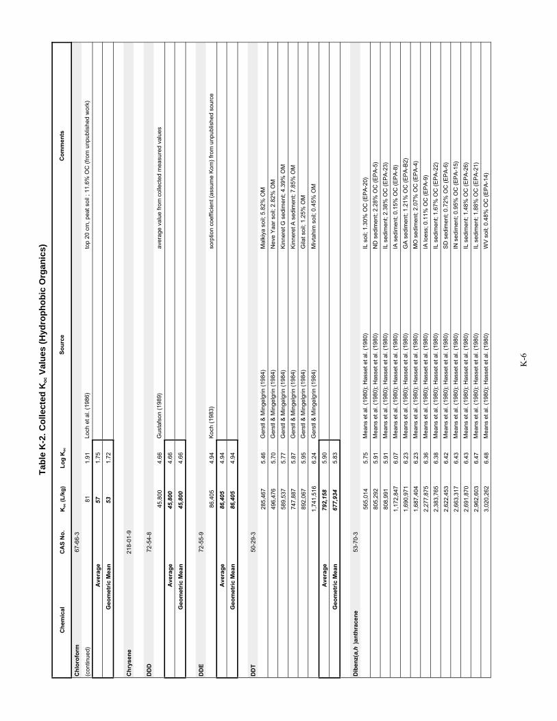
Tab
le K
-2. C
olle
cted
Ko
c Val
ues
(H
ydro
ph
ob
ic O
rgan
ics)
Ch
emic
alC
AS
No
.K
oc
(L/k
g)
Lo
g K
oc
So
urc
eC
om
men
ts
Ch
loro
form
67-6
6-3
(con
tinue
d)81
1.91
Loch
et a
l. (1
986)
top
20 c
m, p
eat s
oil ;
11.
6% O
C (
from
unp
ublis
hed
wor
k)
Ave
rag
e57
1.75
Geo
met
ric
Mea
n53
1.72
Ch
ryse
ne
218-
01-9
DD
D72
-54-
8
45,8
004.
66G
usta
fson
(19
89)
aver
age
valu
e fr
om c
olle
cted
mea
sure
d va
lues
Ave
rag
e45
,800
4.66
Geo
met
ric
Mea
n45
,800
4.66
DD
E72
-55-
9
86,4
054.
94K
och
(198
3)so
rptio
n co
effic
ient
(as
sum
e K
om)
from
unp
ublis
hed
sour
ce
Ave
rag
e86
,405
4.94
Geo
met
ric
Mea
n86
,405
4.94
DD
T50
-29-
3
285,
467
5.46
Ger
stl &
Min
gelg
rin (
1984
)M
alki
ya s
oil;
5.82
% O
M
496,
476
5.70
Ger
stl &
Min
gelg
rin (
1984
)N
eve
Yaa
r so
il; 2
.82%
OM
589,
537
5.77
Ger
stl &
Min
gelg
rin (
1984
)K
inne
ret G
sed
imen
t; 4.
39%
OM
747,
887
5.87
Ger
stl &
Min
gelg
rin (
1984
)K
inne
ret A
sed
imen
t; 7.
85%
OM
892,
067
5.95
Ger
stl &
Min
gelg
rin (
1984
)G
ilat s
oil;
1.25
% O
M
1,74
1,51
66.
24G
erst
l & M
inge
lgrin
(19
84)
Miv
tahi
m s
oil;
0.45
% O
M
Ave
rag
e79
2,15
85.
90
Geo
met
ric
Mea
n67
7,93
45.
83
Dib
enz(
a,h
)an
thra
cen
e53
-70-
3
565,
014
5.75
Mea
ns e
t al.
(198
0); H
asse
t et a
l. (1
980)
IL
soi
l; 1.
30%
OC
(E
PA
-20)
805,
292
5.91
Mea
ns e
t al.
(198
0); H
asse
t et a
l. (1
980)
N
D s
edim
ent;
2.28
% O
C (
EP
A-5
)
808,
991
5.91
Mea
ns e
t al.
(198
0); H
asse
t et a
l. (1
980)
IL
sed
imen
t; 2.
38%
OC
(E
PA
-23)
1,17
2,84
76.
07M
eans
et a
l. (1
980)
; Has
set e
t al.
(198
0)
IA s
edim
ent;
0.15
% O
C (
EP
A-8
)
1,69
0,97
16.
23M
eans
et a
l. (1
980)
; Has
set e
t al.
(198
0)
GA
sed
imen
t; 1.
21%
OC
(E
PA
-B2)
1,68
7,40
46.
23M
eans
et a
l. (1
980)
; Has
set e
t al.
(198
0)
MO
sed
imen
t; 2.
07%
OC
(E
PA
-4)
2,27
7,87
56.
36M
eans
et a
l. (1
980)
; Has
set e
t al.
(198
0)
IA lo
ess;
0.1
1% O
C (
EP
A-9
)
2,38
3,76
56.
38M
eans
et a
l. (1
980)
; Has
set e
t al.
(198
0)
IL s
edim
ent;
1.67
% O
C (
EP
A-2
2)
2,62
2,45
36.
42M
eans
et a
l. (1
980)
; Has
set e
t al.
(198
0)
SD
sed
imen
t; 0.
72%
OC
(E
PA
-6)
2,66
3,31
76.
43M
eans
et a
l. (1
980)
; Has
set e
t al.
(198
0)
IN s
edim
ent;
0.95
% O
C (
EP
A-1
5)
2,69
1,87
06.
43M
eans
et a
l. (1
980)
; Has
set e
t al.
(198
0)
IL s
edim
ent;
1.48
% O
C (
EP
A-2
6)
2,96
2,60
36.
47M
eans
et a
l. (1
980)
; Has
set e
t al.
(198
0)
IL s
edim
ent;
1.88
% O
C (
EP
A-2
1)
3,02
0,26
26.
48M
eans
et a
l. (1
980)
; Has
set e
t al.
(198
0)
WV
soi
l; 0.
48%
OC
(E
PA
-14)
K-6

Tab
le K
-2. C
olle
cted
Ko
c Val
ues
(H
ydro
ph
ob
ic O
rgan
ics)
Ch
emic
alC
AS
No
.K
oc
(L/k
g)
Lo
g K
oc
So
urc
eC
om
men
ts
Dib
enz(
a,h
)an
thra
cen
e53
-70-
3
(con
tinue
d)3,
059,
425
6.49
Mea
ns e
t al.
(198
0); H
asse
t et a
l. (1
980)
K
Y s
edim
ent;
0.66
% O
C (
EP
A-1
8)
Ave
rag
e2,
029,
435
6.31
Geo
met
ric
Mea
n1,
789,
101
6.25
1,2-
Dic
hlo
rob
enze
ne
(o)
95-5
0-1
267
2.43
Lee
et a
l. (1
989)
untr
eate
d M
arle
tte s
oil,
B+
hor
izon
; 0.3
% O
C
280
2.45
Lee
et a
l. (1
989)
untr
eate
d M
arle
tte s
oil,
A h
oriz
on; 2
.59%
OC
310
2.49
Chi
ou e
t al.
(197
9)W
illam
ette
silt
loam
; 0.9
28%
OC
; 3.5
deg
rees
Cel
sius
321
2.51
Chi
ou e
t al.
(198
3)W
oodb
urn
silt
loam
; 1.9
% O
M; 9
% s
and;
68%
silt
; 21%
cla
y
386
2.59
Sta
uffe
r &
Mac
Inty
re (
1986
)A
ppal
ache
e so
rben
t; 1.
4% O
C; p
H =
6.3
438
2.64
Sta
uffe
r &
Mac
Inty
re (
1986
)A
ppal
ache
e so
rben
t; 1.
4% O
C; p
H =
4.1
485
2.69
Frie
sel e
t al.
(198
4)pe
aty
soil;
29%
OM
497
2.70
Piw
oni &
Ban
erje
e (1
989)
sedi
men
t, 0.
19%
OC
; avg
. 2 v
alue
s
529
2.72
Frie
sel e
t al.
(198
4)fo
c re
port
ed a
s a
rang
e; a
vg. o
f sev
eral
exp
er.
Ave
rag
e39
02.
59
Geo
met
ric
Mea
n37
92.
58
1,4-
Dic
hlo
rob
enze
ne
(p)
106-
46-7
273
2.44
Chi
ou e
t al.
(198
3)W
oodb
urn
silt
loam
; fom
= 0
.019
; 21%
cla
y
280
2.45
Sou
thw
orth
& K
elle
r (1
986)
Dor
mon
t soi
l with
1.2
% O
C; 6
0% c
lay
300
2.48
Hut
zler
et a
l. (1
983)
co
lum
n; G
rayl
ing
soil;
1.5
2% O
C; B
21 h
oriz
on
398
2.60
Wils
on e
t al.
(198
1)Li
ncol
n sa
nd; 0
.087
% O
C
429
2.63
Frie
sel e
t al.
(198
4)re
port
ed a
s K
om; f
oc g
iven
as
a ra
nge
603
2.78
Sch
war
zenb
ach
& W
esta
ll (1
981)
K
S1
field
sam
ple;
0.7
3% O
C
665
2.82
Sou
thw
orth
& K
elle
r (1
986)
Api
son
soil
with
0.1
1% O
C; 8
6% c
lay
700
2.85
Hut
zler
et a
l. (1
983)
ba
tch;
ave
rage
of f
ive
soils
724
2.86
Sch
war
zenb
ach
& G
iger
(19
82)
as c
ited
in G
erst
l (19
90)
syst
em s
peci
fic in
form
atio
n no
t pro
vide
d
733
2.87
Sch
war
zenb
ach
& W
esta
ll (1
981)
aver
age
of s
ix m
easu
rem
ents
; aqu
ifer
mat
eria
l; fo
c =
0.0
015
832
2.92
Chi
n &
Web
er (
1989
)hu
mic
aci
d po
lym
ers
850
2.93
Sou
thw
orth
& K
elle
r (1
986)
Ful
lert
on s
oil w
ith 0
.06%
OC
911
2.96
Loch
et a
l. (1
986)
top
20 c
m o
f Eer
d so
il; 0
.06%
OC
; col
umn
1,02
43.
01W
u &
Gsc
hwen
d (1
986)
Cha
rles
Riv
er s
edim
ent;
8.5%
OC
1,25
93.
10S
chw
arze
nbac
h &
Gig
er (
1982
) as
cite
d in
Ger
stl (
1990
) sy
stem
spe
cific
info
rmat
ion
not p
rovi
ded
1,37
53.
14S
chw
arze
nbac
h &
Wes
tall
(198
1)fie
ld s
ampl
e; 0
.08%
OC
Ave
rag
e68
72.
84
Geo
met
ric
Mea
n61
62.
79
3,3-
Dic
hlo
rob
enzi
din
e91
-94-
1
K-7

Tab
le K
-2. C
olle
cted
Ko
c Val
ues
(H
ydro
ph
ob
ic O
rgan
ics)
Ch
emic
alC
AS
No
.K
oc
(L/k
g)
Lo
g K
oc
So
urc
eC
om
men
ts
1,1-
Dic
hlo
roet
han
e75
-34-
3
461.
66Ju
ry e
t al.
(199
0)so
il; s
elec
ted
621.
79R
oy e
t al.
(198
7)co
mpu
ted
from
an
isot
herm
; 4.0
4% O
C
Ave
rag
e54
1.73
Geo
met
ric
Mea
n53
1.73
1,2-
Dic
hlo
roet
han
e10
7-06
-2
221.
34Ju
ry e
t al.
(199
0)so
il; s
elec
ted
331.
52C
hiou
et a
l. (1
979)
Will
amet
te s
ilt lo
am; 0
.928
% O
C; 2
0 de
gree
s C
elsi
us
761.
88W
ilson
et a
l. (1
981)
Linc
oln
sand
; 0.0
87%
OC
Ave
rag
e44
1.64
Geo
met
ric
Mea
n38
1.58
1,1-
Dic
hlo
roet
hyl
ene
75-3
5-4
651.
81S
chw
ille
(198
8) (
seco
ndar
y)
Ave
rag
e65
1.81
Geo
met
ric
Mea
n65
1.81
cis
-1,2
-Dic
hlo
roet
hyl
ene
156-
59-2
tran
s-1
,2-D
ich
loro
eth
ylen
e15
6-60
-5
381.
58B
russ
eau
& R
ao (
1991
)T
ampa
san
dy a
quife
r m
ater
ial;
0.13
% O
C; <
2m
m
Ave
rag
e38
1.58
Geo
met
ric
Mea
n38
1.58
1,2-
Dic
hlo
rop
rop
ane
78-8
7-5
471.
67C
hiou
et a
l. (1
979)
Will
amet
te s
ilt lo
am; 0
.928
% O
C; 2
0 de
gree
s C
elsi
us
Ave
rag
e47
1.67
Geo
met
ric
Mea
n47
1.67
1,3-
Dic
hlo
rop
rop
ene
542-
75-6
241.
38Le
istr
a (1
970)
cis-
, av
g. 3
soi
ls; c
ompu
ted
from
vap
or p
hase
sor
ptio
n
261.
41Le
istr
a (1
970)
tran
s- ,
avg.
3 s
oils
; com
pute
d fr
om v
apor
pha
se s
orpt
ion
321.
51W
auch
ope
et a
l. (1
992)
tran
s-, p
erso
nal c
omm
. (un
publ
ishe
d so
urce
, Dow
Che
mic
al)
Ave
rag
e27
1.44
Geo
met
ric
Mea
n27
1.43
Die
ldri
n60
-57-
1
23,3
084.
37S
haro
m e
t al.
(198
0)B
ever
ly s
andy
loam
; 2.5
% O
M
26,1
064.
42S
haro
m e
t al.
(198
0)P
lain
field
san
d; 0
.7%
OM
27,3
994.
44S
haro
m e
t al.
(198
0)B
ig C
reek
sed
imen
t; 2.
8% O
M
Ave
rag
e25
,604
4.41
Geo
met
ric
Mea
n25
,546
4.41
K-8

Tab
le K
-2. C
olle
cted
Ko
c Val
ues
(H
ydro
ph
ob
ic O
rgan
ics)
Ch
emic
alC
AS
No
.K
oc
(L/k
g)
Lo
g K
oc
So
urc
eC
om
men
ts
Die
thyl
ph
thal
ate
84-6
6-2
691.
84R
usse
ll &
McD
uffie
(19
86)
Bro
ome
Cou
nty,
NY
, com
posi
te s
oil w
ith 1
.59%
OC
; col
umn
981.
99R
usse
ll &
McD
uffie
(19
86)
Con
klin
, NY
, san
d; 0
.26%
OC
; col
umn;
avg
. 4 v
alue
s
Ave
rag
e84
1.92
Geo
met
ric
Mea
n82
1.92
Dim
eth
yl p
hth
alat
e13
1-11
-3
7.6
0.88
Sei
p et
al.
(198
6)fo
rest
soi
l with
0.2
% O
C; c
olum
n st
udy
42.8
1.63
Sei
p et
al.
(198
6)ag
ricul
tura
l soi
l with
2.2
% O
C; c
olum
n st
udy
72.7
1.86
Sei
p et
al.
(198
6)fo
rest
soi
l with
3.7
% O
C; c
olum
n st
udy
Ave
rag
e41
1.61
Geo
met
ric
Mea
n29
1.46
Di-
n-b
uty
l ph
thal
ate
84-7
4-2
1,38
43.
14R
usse
ll &
McD
uffie
(19
86)
Bro
ome
Cou
nty,
NY
, com
posi
te s
oil w
ith 1
.59%
OC
; col
umn
1,77
53.
25R
usse
ll &
McD
uffie
(19
86)
Con
klin
, NY
, san
d; 0
.26%
OC
; ads
orp.
; avg
. 4 v
alue
s; c
olum
n
Ave
rag
e1,
580
3.20
Geo
met
ric
Mea
n1,
567
3.20
2,4-
Din
itro
tolu
ene
121-
14-2
2,6-
Din
itro
tolu
ene
606-
20-2
Di-
n-o
ctyl
ph
thal
ate
117-
84-0
En
do
sulf
an11
5-29
-7
2,04
03.
31G
usta
fson
(19
89)
aver
age
valu
e fr
om c
olle
cted
mea
sure
d va
lues
Ave
rag
e2,
040
3.31
Geo
met
ric
Mea
n2,
040
3.31
En
dri
n72
-20-
8
7,72
43.
89S
haro
m e
t al.
(198
0)B
ever
ly s
andy
loam
; 2.5
% O
M
7,79
33.
89S
haro
m e
t al.
(198
0)or
gani
c so
il; 7
5.3%
OM
14,2
854.
15S
haro
m e
t al.
(198
0)P
lain
field
san
d; 0
.7%
OM
15,8
854.
20S
haro
m e
t al.
(198
0)B
ig C
reek
sed
imen
t; 2.
8% O
M
Ave
rag
e11
,422
4.06
Geo
met
ric
Mea
n10
,811
4.03
Eth
ylb
enze
ne
100-
41-4
165
2.22
Chi
ou e
t al.
(198
3)W
oodb
urn
silt
loam
; fom
= 0
.019
; 21%
cla
y
184
2.27
Lee
et a
l. (1
989)
untr
eate
d S
t. C
lair
soil;
0.4
4% O
C; 4
4% c
lay;
B+
hor
izon
191
2.28
Lee
et a
l. (1
989)
untr
eate
d O
shte
mo
soil;
0.1
1% O
C; 6
.3%
cla
y; B
+ h
oriz
on
240
2.38
Hod
son
& W
illia
ms
(198
8)H
PLC
; cya
nopr
opyl
col
umn
K-9
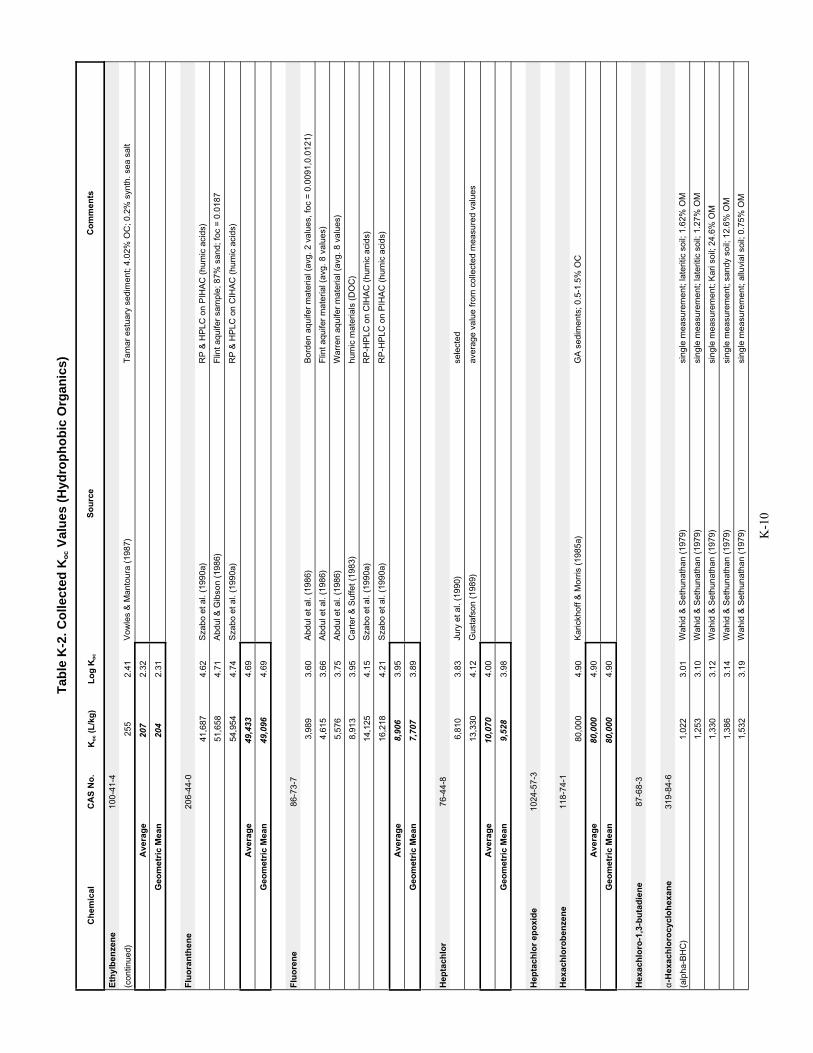
Tab
le K
-2. C
olle
cted
Ko
c Val
ues
(H
ydro
ph
ob
ic O
rgan
ics)
Ch
emic
alC
AS
No
.K
oc
(L/k
g)
Lo
g K
oc
So
urc
eC
om
men
ts
Eth
ylb
enze
ne
100-
41-4
(con
tinue
d)25
52.
41V
owle
s &
Man
tour
a (1
987)
Tam
ar e
stua
ry s
edim
ent;
4.02
% O
C; 0
.2%
syn
th. s
ea s
alt
Ave
rag
e20
72.
32
Geo
met
ric
Mea
n20
42.
31
Flu
ora
nth
ene
206-
44-0
41,6
874.
62S
zabo
et a
l. (1
990a
)R
P &
HP
LC o
n P
IHA
C (
hum
ic a
cids
)
51,6
584.
71A
bdul
& G
ibso
n (1
986)
Flin
t aqu
ifer
sam
ple;
87%
san
d; fo
c =
0.0
187
54,9
544.
74S
zabo
et a
l. (1
990a
)R
P &
HP
LC o
n C
IHA
C (
hum
ic a
cids
)
Ave
rag
e49
,433
4.69
Geo
met
ric
Mea
n49
,096
4.69
Flu
ore
ne
86-7
3-7
3,98
93.
60A
bdul
et a
l. (1
986)
Bor
den
aqui
fer
mat
eria
l (av
g. 2
val
ues,
foc
= 0
.009
1,0.
0121
)
4,61
53.
66A
bdul
et a
l. (1
986)
Flin
t aqu
ifer
mat
eria
l (av
g. 8
val
ues)
5,57
63.
75A
bdul
et a
l. (1
986)
War
ren
aqui
fer
mat
eria
l (av
g. 8
val
ues)
8,91
33.
95C
arte
r &
Suf
fet (
1983
)hu
mic
mat
eria
ls (
DO
C)
14,1
254.
15S
zabo
et a
l. (1
990a
)R
P-H
PLC
on
CIH
AC
(hu
mic
aci
ds)
16,2
184.
21S
zabo
et a
l. (1
990a
)R
P-H
PLC
on
PIH
AC
(hu
mic
aci
ds)
Ave
rag
e8,
906
3.95
Geo
met
ric
Mea
n7,
707
3.89
Hep
tach
lor
76-4
4-8
6,81
03.
83Ju
ry e
t al.
(199
0)se
lect
ed
13,3
304.
12G
usta
fson
(19
89)
aver
age
valu
e fr
om c
olle
cted
mea
sure
d va
lues
Ave
rag
e10
,070
4.00
Geo
met
ric
Mea
n9,
528
3.98
Hep
tach
lor
epo
xid
e10
24-5
7-3
Hex
ach
loro
ben
zen
e11
8-74
-1
80,0
004.
90K
aric
khof
f & M
orris
(19
85a)
GA
sed
imen
ts; 0
.5-1
.5%
OC
Ave
rag
e80
,000
4.90
Geo
met
ric
Mea
n80
,000
4.90
Hex
ach
loro
-1,3
-bu
tad
ien
e87
-68-
3
α-H
exac
hlo
rocy
clo
hex
ane
319-
84-6
(alp
ha-B
HC
)1,
022
3.01
Wah
id &
Set
huna
than
(19
79)
sing
le m
easu
rem
ent;
late
ritic
soi
l; 1.
62%
OM
1,25
33.
10W
ahid
& S
ethu
nath
an (
1979
) si
ngle
mea
sure
men
t; la
terit
ic s
oil;
1.27
% O
M
1,33
03.
12W
ahid
& S
ethu
nath
an (
1979
) si
ngle
mea
sure
men
t; K
ari s
oil;
24.6
% O
M
1,38
63.
14W
ahid
& S
ethu
nath
an (
1979
) si
ngle
mea
sure
men
t; sa
ndy
soil;
12.
6% O
M
1,53
23.
19W
ahid
& S
ethu
nath
an (
1979
) si
ngle
mea
sure
men
t; al
luvi
al s
oil;
0.75
% O
M
K-1
0

Tab
le K
-2. C
olle
cted
Ko
c Val
ues
(H
ydro
ph
ob
ic O
rgan
ics)
Ch
emic
alC
AS
No
.K
oc
(L/k
g)
Lo
g K
oc
So
urc
eC
om
men
ts
α-H
exac
hlo
rocy
clo
hex
ane
319-
84-6
(con
tinue
d)2,
004
3.30
Wah
id &
Set
huna
than
(19
79)
sing
le m
easu
rem
ent;
late
ritic
soi
l; 2.
88%
OM
2,02
43.
31W
ahid
& S
ethu
nath
an (
1979
) si
ngle
mea
sure
men
t; la
terit
ic s
oil;
1.00
% O
M
2,09
03.
32W
ahid
& S
ethu
nath
an (
1979
) si
ngle
mea
sure
men
t; P
okka
li so
il; 5
.52%
OM
2,12
33.
33W
ahid
& S
ethu
nath
an (
1979
) si
ngle
mea
sure
men
t; K
ari s
oil;
8.21
% O
M
2,16
83.
34W
ahid
& S
ethu
nath
an (
1979
) si
ngle
mea
sure
men
t; la
terit
ic s
oil;
0.60
% O
M
2,20
03.
34W
ahid
& S
ethu
nath
an (
1979
) si
ngle
mea
sure
men
t; la
terit
ic s
oil;
0.92
% O
M
2,89
13.
46W
ahid
& S
ethu
nath
an (
1979
) si
ngle
mea
sure
men
t; al
luvi
al s
oil;
0.70
% O
M
Ave
rag
e1,
835
3.26
Geo
met
ric
Mea
n1,
762
3.25
β-H
exac
hlo
rocy
clo
hex
ane
319-
85-7
(bet
a-B
HC
)1,
156
3.06
Wah
id &
Set
huna
than
(19
79)
sing
le m
easu
rem
ent;
late
ritic
soi
l; 1.
27%
OM
1,47
03.
17W
ahid
& S
ethu
nath
an (
1979
)si
ngle
mea
sure
men
t; la
terit
ic s
oil;
1.62
% O
M
1,68
13.
23W
ahid
& S
ethu
nath
an (
1979
)si
ngle
mea
sure
men
t; K
ari s
oil;
24.6
% O
M
1,79
43.
25M
ills
& B
igga
r (1
969b
)V
enad
o cl
ay; 3
.5%
OC
; 50%
mon
tmor
illon
ite; 2
0°
C; 1
/n=
0.86
1
1,82
13.
26W
ahid
& S
ethu
nath
an (
1979
)si
ngle
mea
sure
men
t; sa
ndy
soil;
12.
6% O
M
1,86
83.
27W
ahid
& S
ethu
nath
an (
1979
)si
ngle
mea
sure
men
t; la
terit
ic s
oil;
1.00
% O
M
1,95
83.
29W
ahid
& S
ethu
nath
an (
1979
)si
ngle
mea
sure
men
t; al
luvi
al s
oil;
0.75
% O
M
2,09
83.
32W
ahid
& S
ethu
nath
an (
1979
)si
ngle
mea
sure
men
t; al
luvi
al s
oil;
0.70
% O
M
2,41
53.
38W
ahid
& S
ethu
nath
an (
1979
)si
ngle
mea
sure
men
t; K
ari s
oil;
8.21
% O
M
2,54
83.
41W
ahid
& S
ethu
nath
an (
1979
)si
ngle
mea
sure
men
t; la
terit
ic s
oil;
0.60
% O
M
2,69
73.
43W
ahid
& S
ethu
nath
an (
1979
)si
ngle
mea
sure
men
t; la
terit
ic s
oil;
0.92
% O
M
3,14
33.
50W
ahid
& S
ethu
nath
an (
1979
)si
ngle
mea
sure
men
t; la
terit
ic s
oil;
2.88
% O
M
3,15
83.
50W
ahid
& S
ethu
nath
an (
1979
)si
ngle
mea
sure
men
t; P
okka
li so
il; 5
.52%
OM
3,56
33.
55M
ills
& B
igga
r (1
969b
)S
tate
n pe
aty
muc
k, 1
2.8%
OC
; 20
° C
; 1/n
= 0
.950
Ave
rag
e2,
241
3.35
Geo
met
ric
Mea
n2,
139
3.33
γ-H
exac
hlo
rocy
clo
hex
ane
58-8
9-9
(Lin
dane
)73
12.
86A
dam
s &
Li (
1971
)S
vea
sil,
A h
oriz
on ;
foc
= 0
.031
735
2.87
McC
all e
t al.
(198
0)av
erag
e fo
r th
ree
soils
, 0.6
8-2.
01%
OC
757
2.88
Hug
genb
erge
r et
al.
(197
2)G
ila s
ilt lo
am; f
oc =
0.0
038;
cou
lmn
stud
y
760
2.88
Kis
hi e
t al.
(199
0)cl
ay lo
am (
allo
phan
e); s
oil p
H =
4.8
9; fo
c =
0.1
04
760
2.88
Wah
id &
Set
huna
than
(19
80)
late
rtic
soi
l; 2.
88%
OM
; 1:1
764
2.88
Ada
ms
& L
i (19
71)
Heg
ne s
ic, A
hor
izon
; fo
c =
0.0
43
764
2.88
Ada
ms
& L
i (19
71)
Heg
ne s
ic, B
hor
izon
; fo
c =
0.0
06
769
2.89
Ada
ms
& L
i (19
71)
Far
go s
ic, A
hor
izon
; fo
c =
0.0
52
812
2.91
Ada
ms
& L
i (19
71)
Hub
bard
ls, A
hor
izon
; fo
c =
0.0
12
814
2.91
Ada
ms
& L
i (19
71)
Ont
onag
on c
, A h
oriz
on ;
foc
= 0
.035
826
2.92
Ada
ms
& L
i (19
71)
Mila
ca s
l, A
hor
izon
; fo
c =
0.0
17
852
2.93
Mill
s &
Big
gar
(196
9a)
1.1%
OC
; Ca
Col
umbi
a si
lt lo
am
K-1
1

Tab
le K
-2. C
olle
cted
Ko
c Val
ues
(H
ydro
ph
ob
ic O
rgan
ics)
Ch
emic
alC
AS
No
.K
oc
(L/k
g)
Lo
g K
oc
So
urc
eC
om
men
ts
γ-H
exac
hlo
rocy
clo
hex
ane
58-8
9-9
(con
tinue
d)85
52.
93A
dam
s &
Li (
1971
)K
ranz
burg
sic
l, B
hor
izon
; fo
c =
0.0
1
878
2.94
Ada
ms
& L
i (19
71)
Sve
a si
l, B
hor
izon
; fo
c =
0.0
08
960
2.98
Kis
hi e
t al.
(199
0)sa
ndy
loam
(al
loph
ane)
; soi
l pH
= 5
.41;
foc
= 0
.079
1
968
2.99
Kay
& E
lrick
(19
67)
Muc
k (3
8% O
C)
985
2.99
Ada
ms
& L
i (19
71)
Fay
ette
sil,
A h
oriz
on ;
foc
= 0
.023
986
2.99
Kay
& E
lrick
(19
67)
Hon
eyw
ood
loam
(2.
1% O
C)
1,00
53.
00A
dam
s &
Li (
1971
)C
anis
teo
cl, B
hor
izon
; fo
c =
0.0
06
1,01
03.
00R
ippe
n et
al.
(198
2)A
lfiso
l; U
dalf,
Par
a br
own
eart
h; 0
.76%
OC
; soi
l pH
= 7
.45
1,03
03.
01K
ay &
Elri
ck (
1967
)F
ox lo
amy
sand
(1.
7% O
C)
1,07
93.
03A
dam
s &
Li (
1971
)Le
ster
fsl,
A h
oriz
on ;
foc
= 0
.023
1,10
33.
04H
ugge
nber
ger
et a
l. (1
972)
Pac
happ
a sa
ndy
loam
; foc
= 0
.005
1,10
33.
04S
haro
m e
t al.
(198
0)B
ever
ly s
and
loam
; 2.5
% O
M
1,10
93.
04W
ahid
& S
ethu
nath
an (
1979
)si
ngle
mea
sure
men
t; sa
ndy
soil;
12.
6% O
C
1,12
53.
05A
dam
s &
Li (
1971
)Z
imm
erm
an s
, A h
oriz
on ;
foc
= 0
.007
1,13
03.
05H
ugge
nber
ger
et a
l. (1
972)
Ken
twoo
d sa
ndy
loam
; foc
= 0
.009
3
1,20
03.
08K
ishi
et a
l. (1
990)
light
cla
y (m
ontm
orill
onite
- il
lite)
; pH
= 5
.26;
foc
= 0
.032
3
1,20
43.
08W
ahid
& S
ethu
nath
an (
1979
)si
ngle
mea
sure
men
t; la
terit
ic s
oil;
1.27
% O
M
1,22
73.
09K
ay &
Elri
ck (
1967
)B
rook
ston
e sa
ndy
loam
(1.
9% O
C)
1,26
33.
10A
dam
s &
Li (
1971
)B
rain
erd
fsl,
A h
oriz
on ;
foc
= 0
.026
1,27
43.
11A
dam
s &
Li (
1971
)B
eard
en s
il, B
hor
izon
; fo
c =
0.0
02
1,30
03.
11K
ishi
et a
l. (1
990)
light
cla
y (m
ontm
orill
onite
); s
oil p
H =
5.1
8; fo
c =
0.0
151
1,30
03.
11M
cCal
l et a
l. (1
983)
Not
sta
ted
if th
ese
are
orig
inal
dat
a
1,31
83.
12M
iller
& W
eber
(19
86)
Ann
Arb
or s
oil;
1.14
% O
C
1,32
23.
12M
orea
le &
van
Bla
del (
1978
)Lu
bbee
k II
soil;
0.5
3% O
C; 1
0% c
lay
1,33
53.
13M
orea
le &
van
Bla
del (
1978
)Lu
bbee
k I s
oil;
0.07
% O
C; 2
% c
lay
1,45
23.
16M
ills
& B
igga
r (1
969a
) 3.
1% O
C; C
a V
enad
o cl
ay
1,45
53.
16A
dam
s &
Li (
1971
)B
rain
erd
sl, B
hor
izon
; fo
c =
0.0
01
1,45
83.
16M
iller
& W
eber
(19
86)
Del
ta s
oil;
0.12
% T
OC
1,47
83.
17S
haro
m e
t al.
(198
0)B
ig C
reek
sed
imen
t; 2.
8% O
M
1,52
53.
18W
ahid
& S
ethu
nath
an (
1978
)P
okka
li so
il; 5
.52%
OM
; 1:1
0; 5
min
eq.
1,58
03.
20W
ahid
& S
ethu
nath
an (
1980
)P
okka
li so
il; 5
.52%
OM
; 1:1
1,68
13.
23W
ahid
& S
ethu
nath
an (
1979
)si
ngle
mea
sure
men
t; K
ari s
oil;
24.6
% O
M
1,72
43.
24W
ahid
& S
ethu
nath
an (
1979
)si
ngle
mea
sure
men
t; la
terit
ic s
oil;
1.00
% O
M
1,83
03.
26A
dam
s &
Li (
1971
)B
lue
Ear
th s
il, A
hor
izon
; fo
c =
0.1
1
1,85
93.
27C
aron
et a
l. (1
985)
Pow
ervi
lle s
edim
ent (
NJ)
; 2-4
% O
C
1,89
63.
28W
ahid
& S
ethu
nath
an (
1979
)si
ngle
mea
sure
men
t; la
terit
ic s
oil;
2.88
% O
M
1,93
53.
29W
ahid
& S
ethu
nath
an (
1979
)si
ngle
mea
sure
men
t; al
luvi
al s
oil;
0.70
% O
M
1,97
03.
29S
haro
m e
t al.
(198
0)P
lain
field
san
d; 0
.7%
OM
1,97
63.
30W
ahid
& S
ethu
nath
an (
1979
)si
ngle
mea
sure
men
t; la
terit
ic s
oil;
1.62
% O
M
2,05
83.
31S
haro
m e
t al.
(198
0)or
gani
c so
il; 7
5.3%
OM
2,09
03.
32W
ahid
& S
ethu
nath
an (
1979
)si
ngle
mea
sure
men
t; P
okka
li so
il; 5
.52%
OM
2,12
23.
33W
ahid
& S
ethu
nath
an (
1979
)si
ngle
mea
sure
men
t; al
luvi
al s
oil;
0.75
% O
M
K-1
2

Tab
le K
-2. C
olle
cted
Ko
c Val
ues
(H
ydro
ph
ob
ic O
rgan
ics)
Ch
emic
alC
AS
No
.K
oc
(L/k
g)
Lo
g K
oc
So
urc
eC
om
men
ts
γ-H
exac
hlo
rocy
clo
hex
ane
58-8
9-9
(con
tinue
d)2,
123
3.33
Wah
id &
Set
huna
than
(19
79)
sing
le m
easu
rem
ent;
Kar
i soi
l; 8.
21%
OM
2,26
03.
35S
penc
er &
Clia
th (
1970
)G
ila s
ilt lo
am; 0
.35%
OC
; fro
m v
apor
pha
se d
esor
p.; 3
0° C
2,26
83.
36A
dam
s &
Li (
1971
)B
lue
Ear
th s
il, B
hor
izon
; fo
c =
0.0
83
2,29
03.
36W
ahid
& S
ethu
nath
an (
1979
)si
ngle
mea
sure
men
t; la
terit
ic s
oil;
0.92
% O
M
2,44
83.
39W
ahid
& S
ethu
nath
an (
1979
)si
ngle
mea
sure
men
t; la
terit
ic s
oil;
0.60
% O
M
2,58
43.
41M
ills
& B
igga
r (1
969a
)11
.9%
OC
; Sta
ten
peat
y m
uck
2,64
63.
42M
iller
& W
eber
(19
86)
Mic
hayw
e so
il; 0
.13%
TO
C
2,71
03.
43M
orea
le &
van
Bla
del (
1978
)Z
olde
r so
il; 0
.19%
OC
; 1%
cla
y
2,92
63.
47W
ahid
& S
ethu
nath
an (
1978
)al
luvi
al s
oil;
0.75
% O
M; 1
:20;
5 m
in e
qulib
ratio
n
2,98
33.
47C
hiou
et a
l. (1
979)
Will
amet
te s
ilt lo
am; 1
.6%
OM
; 26%
cla
y
3,24
93.
51A
dam
s &
Li (
1971
)U
len
sl, B
hor
izon
; fo
c =
0.0
03
Ave
rag
e1,
477
3.17
Geo
met
ric
Mea
n1,
352
3.13
Hex
ach
loro
cycl
op
enta
die
ne
77-4
7-4
Hex
ach
loro
eth
ane
67-7
2-1
Ind
eno
(1,2
,3-c
d)p
yren
e19
3-39
-5
Iso
ph
oro
ne
78-5
9-1
(Iso
octa
phen
one)
Met
ho
xych
lor
72-4
3-5
80,0
004.
90K
aric
khof
f et a
l. (1
979)
avg.
Doe
Run
and
Hic
kory
Hill
coa
rse
silt
sed.
frac
tions
Ave
rag
e80
,000
4.90
Geo
met
ric
Mea
n80
,000
4.90
Met
hyl
bro
mid
e74
-83-
9
(Bro
mom
etha
ne)
90.
95B
riggs
(19
81)
pres
ente
d as
a v
alue
for
seve
ral c
hem
ical
s
Ave
rag
e9
0.95
Geo
met
ric
Mea
n9
0.95
Met
hyl
ch
lori
de
75-0
9-2
(chl
orom
etha
ne)
60.
78Ju
ry e
t al.
(199
0)so
il; s
elec
ted
Ave
rag
e6
0.78
Geo
met
ric
Mea
n6
0.78
Met
hyl
ene
chlo
rid
e75
-09-
2
(Dic
hlor
omet
hane
)10
1.00
Dan
iels
et a
l. (1
985)
sele
cted
Ave
rag
e10
1.00
Geo
met
ric
Mea
n10
1.00
K-1
3

Tab
le K
-2. C
olle
cted
Ko
c Val
ues
(H
ydro
ph
ob
ic O
rgan
ics)
Ch
emic
alC
AS
No
.K
oc
(L/k
g)
Lo
g K
oc
So
urc
eC
om
men
ts
Nap
hth
alen
e91
-20-
3
830
2.92
Kis
hi e
t al.
(199
0)lig
ht c
lay;
1.5
1% O
C
843
2.93
Vow
les
& M
anto
ura
(198
7)T
amar
est
uary
sed
imen
t; 4.
02%
OC
; 0.2
% s
ynth
. sea
sal
t
871
2.94
Kar
ickh
off (
1981
)so
ils/s
edim
ents
ave
rage
; sha
ke fl
ask
UV
907
2.96
Sta
uffe
r &
Mac
Inty
re (
1986
)A
ppal
ache
e so
il; 1
.4%
OC
; pH
= 3
.1
912
2.96
Hod
son
& W
illia
ms
(198
8)un
publ
ishe
d ex
perim
enta
l res
ults
by
sam
e au
thor
s
960
2.98
Sou
thw
orth
& K
elle
r (1
986)
Ful
lert
on s
oil;
0.06
% O
C
1,00
03.
00S
outh
wor
th &
Kel
ler
(198
6)A
piso
n so
il; 0
.11%
OC
1,00
03.
00K
an &
Tom
son
(199
0)D
OM
1,09
63.
04M
cCar
thy
& J
imin
ez (
1985
)hu
mic
aci
d po
lym
ers
1,16
13.
06Lo
kke
(198
4)av
g. 1
0 va
lues
1,29
03.
11R
ippe
n et
al.
(198
2)A
lfiso
l; 0.
76%
OC
1,30
03.
11K
aric
khof
f et a
l. (1
979)
aver
age
of D
oe R
un &
Hic
kory
Hill
sed
imen
ts
1,33
33.
12K
aric
khof
f (19
82)
Mis
siss
ippi
Riv
er s
edim
ent;
foc
= 0
.015
1,40
03.
15P
odol
l et a
l. (1
989)
Men
lo P
ark
soil;
1.6
% O
C
1,41
33.
15S
zabo
et a
l. (1
990a
)R
P-H
PLC
on
CIH
AC
(hu
mic
aci
ds)
1,44
03.
16R
ippe
n et
al.
(198
2)E
ntis
ol; 1
.11%
OC
1,44
53.
16S
zabo
et a
l. (1
990a
)R
P-H
PLC
on
PIH
AC
(hu
mic
aci
ds)
1,61
03.
21R
ippe
n et
al.
(198
2)S
peye
r so
il, 0
.15-
0.5
mm
; 1.1
2% O
C
1,86
13.
27B
arre
tt et
al.
(199
4)so
il; 0
.13%
OC
1,95
03.
29W
ood
et a
l. (1
990)
Eus
tis s
and;
0.7
4% O
C; b
atch
& c
olum
n da
ta
Ave
rag
e1,
231
3.09
Geo
met
ric
Mea
n1,
191
3.08
Nit
rob
enze
ne
98-9
5-3
30.6
1.49
Sei
p et
al.
(198
6)fo
rest
soi
l with
0.2
% O
C; c
olum
n st
udy
761.
88W
ilson
et a
l. (1
981)
Linc
oln
sand
; 0.0
87%
OC
861.
93B
riggs
(19
81)
aver
age
for
four
soi
ls; 0
.6-2
.5%
OC
88.8
1.95
Sei
p et
al.
(198
6)ag
ricul
tura
l soi
l with
2.2
% O
C; c
olum
n st
udy
103
2.01
Sei
p et
al.
(198
6)fo
rest
soi
l with
3.7
% O
C; c
olum
n st
udy
142
2.15
Mill
er &
Web
er (
1986
)D
elta
soi
l with
foc
= 0
.001
2
190
2.28
Lokk
e (1
984)
Grib
skov
B h
oriz
on s
oil;
2.58
%O
C; a
vg. 2
val
ues
191
2.28
Wils
on e
t al.
(198
1)Li
ncol
n sa
nd; 0
.087
% O
C
229
2.36
Hod
son
& W
illia
ms
(198
8)un
publ
ishe
d ex
perim
enta
l res
ults
by
sam
e au
thor
s
270
2.43
Lokk
e (1
984)
Grib
skov
C h
oriz
on s
oil;
1.82
%O
C; a
vg. 2
val
ues
Ave
rag
e14
12.
15
Geo
met
ric
Mea
n11
92.
08
Pen
tach
loro
ben
zen
e60
8-93
-5
11,3
814.
06W
u &
Gsc
hwen
d (1
986)
Iow
a so
il; 2
.1%
OC
35,4
554.
55W
u &
Gsc
hwen
d (1
986)
Nor
th R
iver
sed
imen
ts; a
ppro
x. 4
.4%
OC
38,5
604.
59B
arbe
r et
al.
(199
2)sa
nd/g
rave
l aqu
ifer;
avg
, 2 m
easu
rem
ents
; 0.0
54, 0
.062
% O
C
40,0
004.
60K
aric
khof
f & M
orris
(19
85a)
GA
sed
imen
ts; 0
.5-1
.5%
OC
K-1
4

Tab
le K
-2. C
olle
cted
Ko
c Val
ues
(H
ydro
ph
ob
ic O
rgan
ics)
Ch
emic
alC
AS
No
.K
oc
(L/k
g)
Lo
g K
oc
So
urc
eC
om
men
ts
Pen
tach
loro
ben
zen
e60
8-93
-5
(con
tinue
d)55
,176
4.74
Wu
& G
schw
end
(198
6)C
harle
s R
iver
sed
imen
ts; a
ppro
x. 8
.5%
OC
Ave
rag
e36
,114
4.56
Geo
met
ric
Mea
n32
,148
4.51
Pyr
ene
129-
00-0
43,8
074.
64M
eans
et a
l. (1
980)
IL s
edim
ent w
ith 2
.38%
OC
(E
PA
-23)
45,7
094.
66A
bdul
et a
l. (1
987)
aqui
fer
mat
eria
l, 1.
05%
OC
48,2
364.
68M
eans
et a
l. (1
980)
IL s
edim
ent w
ith 1
.67%
OC
(E
PA
-22)
50,6
504.
70M
eans
et a
l. (1
980)
ND
sed
imen
t with
2.2
8% O
C (
EP
A-5
)
51,4
694.
71M
eans
et a
l. (1
980)
ND
sed
imen
t with
2.0
7% O
C (
EP
A-4
)
54,7
674.
74W
oodb
urn
et a
l. (1
989)
Web
ster
soi
l; 2.
23%
OC
; 14
C; 3
0:70
met
hano
l:wat
er
57,7
634.
76M
eans
et a
l. (1
980)
WV
soi
l with
0.4
8% O
C (
EP
A-1
4)
58,8
844.
77S
zabo
et a
l. (1
990a
)R
P-H
PLC
on
PIH
AC
(hu
mic
aci
ds)
59,5
154.
77M
eans
et a
l. (1
980)
IL s
edim
ent w
ith 1
.88%
OC
(E
PA
-21)
59,6
464.
78M
eans
et a
l. (1
980)
IL s
oil w
ith 1
.30%
OC
(E
PA
-20)
61,9
364.
79A
bdul
& G
ibso
n (1
986)
Flin
t aqu
ifer
sam
ple;
87%
san
d; fo
c =
0.0
187
62,8
604.
80M
eans
et a
l. (1
980)
GA
sed
imen
t with
1.2
1% O
C (
EP
A-B
2)
63,4
004.
80H
asse
tt et
al.
(198
0)fr
om r
egre
ssio
n of
14
sedi
men
ts/s
oil s
ampl
es
64,7
064.
81M
eans
et a
l. (1
980)
IA lo
ess
with
0.1
1% O
C (
EP
A-9
)
66,0
694.
82S
zabo
et a
l. (1
990a
)R
P-H
PLC
on
CIH
AC
(hu
mic
aci
ds)
67,1
894.
83M
eans
et a
l. (1
980)
IL s
edim
ent w
ith 1
.48%
OC
(E
PA
-26)
67,4
674.
83M
eans
et a
l. (1
980)
IA s
edim
ent w
ith 0
.15%
OC
(E
PA
-8)
67,6
084.
83K
aric
khof
f (19
81)
soils
/sed
imen
ts a
vera
ge
76,3
164.
88M
eans
et a
l. (1
980)
KY
sed
imen
t with
0.6
6% O
C (
EP
A-1
8)
82,4
214.
92M
eans
et a
l. (1
980)
IN s
edim
ent w
ith 0
.95%
OC
(E
PA
-15)
84,0
004.
92K
aric
khof
f et a
l. (1
979)
avg.
Doe
Run
, Hic
kory
Hill
coa
rse
silt
sedi
men
t fra
ctio
ns
84,0
004.
92K
aric
khof
f (19
82)
Mis
siss
ippi
R. s
edim
ent,
1.5%
OC
85,2
564.
93M
eans
et a
l. (1
980)
SD
sed
imen
t with
0.7
2% O
C (
EP
A-6
)
87,8
334.
94K
aric
khof
f & M
orris
(19
85b)
Mis
siss
ippi
R. s
edim
ent,
1.48
% O
C (
deso
rptio
n)
95,3
954.
98K
aric
khof
f & M
orris
(19
85b)
Ohi
o R
. sed
imen
t; 3.
04%
OC
(de
sorp
tion)
131,
325
5.12
Gau
thie
r et
al.
(198
6)flu
ores
c. q
uenc
h. te
ch.;
13 s
oil h
umic
& fu
lvic
aci
ds (
avg.
)
133,
590
5.13
Vow
les
& M
anto
ura
(198
7)T
amar
est
uary
sed
imen
t; 4.
02%
OC
; 0.2
% s
ynth
. sea
sal
t
Ave
rag
e70
,808
4.85
Geo
met
ric
Mea
n67
,992
4.83
Str
yen
e10
0-42
-5
912
2.96
Bed
ient
et a
l. (1
983)
as
cite
d in
Mey
lan
et a
l. (1
992)
ex
perim
enta
l mea
sure
men
t
Ave
rag
e91
22.
96
Geo
met
ric
Mea
n91
22.
96
K-1
5

Tab
le K
-2. C
olle
cted
Ko
c Val
ues
(H
ydro
ph
ob
ic O
rgan
ics)
Ch
emic
alC
AS
No
.K
oc
(L/k
g)
Lo
g K
oc
So
urc
eC
om
men
ts
1,1,
2,2-
Tet
rach
loro
eth
ane
79-3
4-5
791.
90C
hiou
et a
l. (1
979)
Will
amet
te s
ilt lo
am; 0
.928
% O
C; 2
0 de
gree
s C
elsi
us
Ave
rag
e79
1.90
Geo
met
ric
Mea
n79
1.90
Tet
rach
loro
eth
ylen
e12
7-18
-4
177
2.25
Sei
p et
al.
(198
6)fo
rest
soi
l with
0.2
% O
C; c
olum
n st
ufy
205
2.31
Sei
p et
al.
(198
6)ag
ricul
tura
l soi
l wtih
2.2
% O
C; c
olum
n st
udy
224
2.35
Sch
war
zenb
ach
& G
iger
(19
82)
as c
ited
in G
erst
l (19
90)
spec
ific
syst
em in
form
atio
n no
t pro
vide
d
224
2.35
Piw
oni &
Ban
erje
e (1
989)
n-
core
sed
imen
t; fo
c =
0.0
133
225
2.35
Wils
on e
t al.
(198
1)Li
ncol
n sa
nd; 0
.087
% O
C
235
2.37
Piw
oni &
Ban
erje
e (1
989)
av
g. 8
val
ues;
J-c
ore
sed.
; foc
= 0
.001
5 -
0.00
89; a
vg. 1
/n>
0.94
237
2.38
Frie
sel e
t al.
(198
4)re
port
ed a
s K
som
; foc
rep
orte
d as
a r
ange
; 32
soils
263
2.42
Abd
ul e
t al.
(198
7)eq
uilib
rium
bat
ch e
xper
imen
ts; a
quife
r m
ater
ial;
foc
= 0
.010
5
268
2.43
Pig
nate
llo (
1990
)A
gaw
am fi
ne s
andy
loam
soi
l; 2
.57%
OC
; avg
. 2 v
alue
s
269
2.43
Bru
ssea
u &
Rao
(19
91)
Tam
pa s
andy
aqu
ifer
mat
eria
l; 0.
13%
OC
; < 2
mm
311
2.49
Loch
et a
l. (1
986)
top
20 c
m o
f Pod
zol s
oil;
0.87
% O
C
348
2.54
Sei
p et
al.
(198
6)fo
rest
soi
l with
3.7
% O
C; c
olum
n st
udy
356
2.55
Pav
iost
athi
s &
Mat
hava
n (1
992)
coar
se s
and
with
0.0
9% O
C
362
2.56
Chi
ou e
t al.
(197
9)W
illam
ette
silt
loam
; 0.9
3% O
C; 2
0 de
gree
s C
elsi
us
373
2.57
Sch
war
zenb
ach
& W
esta
ll (1
981)
avg.
of 6
mea
s. w
/ diff
eren
t Co
& s
orbe
nts;
0.1
5% O
C
Ave
rag
e27
22.
43
Geo
met
ric
Mea
n26
52.
42
To
luen
e10
8-88
-3
94.4
1.97
Sei
p et
al.
(198
6)ag
ricul
tura
l soi
l wtih
2.2
% O
C; c
olum
n st
udy
992.
00V
owle
s &
Man
tour
a (1
987)
Tam
ar e
stua
ry s
edim
ent;
4.02
% O
C; 0
.2%
syn
th. s
ea s
alt
115
2.06
Abd
ul e
t al.
(198
7)eq
uilib
rium
bat
ch e
xper
imen
ts, a
quife
r m
ater
ial;
foc
= 0
.010
5
123
2.09
Gar
barin
i & L
ion
(198
6)ze
in; 5
7% O
C
126
2.10
Sza
bo e
t al.
(199
0a)
RP
-HP
LC o
n P
IHA
C (
avg.
, hum
ic a
cids
)
134
2.13
Sei
p et
al.
(198
6)fo
rest
soi
l with
3.7
% O
C; c
olum
n st
udy
150
2.18
Wils
on e
t al.
(198
1)Li
ncol
n sa
nd; 0
.087
% O
C
151
2.18
Gar
barin
i & L
ion
(198
6)S
apsu
cker
Woo
ds s
oil w
ith 7
.51%
C
151
2.18
Gar
barin
i & L
ion
(198
6)lig
nin;
65%
OC
164
2.21
Gar
barin
i & L
ion
(198
6)S
apsu
cker
Woo
ds e
ther
ext
ract
ed s
oil w
ith 7
.05%
C
182
2.26
Sza
bo e
t al.
(199
0a)
RP
-HP
LC o
n C
IHA
C (
avg.
, hum
ic a
cids
)
247
2.39
Sch
war
zenb
ach
& W
esta
ll (1
981)
avg.
of 6
mea
s. w
/ diff
eren
t Co
& s
orbe
nts;
0.1
5% O
C
Ave
rag
e14
52.
16
Geo
met
ric
Mea
n14
02.
15
K-1
6

Tab
le K
-2. C
olle
cted
Ko
c Val
ues
(H
ydro
ph
ob
ic O
rgan
ics)
Ch
emic
alC
AS
No
.K
oc
(L/k
g)
Lo
g K
oc
So
urc
eC
om
men
ts
To
xap
hen
e80
01-3
5-2
95,8
164.
98G
usta
fson
(19
89)
aver
age
valu
e fr
om c
olle
cted
mea
sure
d va
lues
Ave
rag
e95
,816
4.98
Geo
met
ric
Mea
n95
,816
4.98
1,2,
4-T
rich
loro
ben
zen
e12
0-82
-1
864
2.94
Chi
ou e
t al.
(198
3)W
oodb
urn
silt
loam
; fom
= 0
.019
; 21%
cla
y
885
2.95
Sou
thw
orth
& K
elle
r (1
986)
Dor
mon
t soi
l; 1.
2% O
C
1,03
33.
01S
cheu
nert
et a
l. (1
994)
soil;
2.0
6% O
C
1,30
03.
11S
outh
wor
th &
Kel
ler
(198
6)F
ulle
rton
soi
l; 0.
06%
OC
1,30
33.
11B
aner
jee
et a
l. (1
985)
aver
age
of 2
1 va
lues
; sub
surf
ace
allu
vial
soi
l
1,38
93.
14W
ilson
et a
l. (1
981)
av
erag
e of
two
valu
es
1,43
53.
16F
riese
l et a
l. (1
984)
peat
y so
il; 0
.29%
OM
1,44
13.
16F
riese
l et a
l. (1
984)
repo
rted
as
Kso
m; f
oc r
epor
ted
as a
ran
ge
1,55
43.
19Le
e et
al.
(198
9)un
trea
ted
Mar
lette
soi
l, A
hor
izon
; 2.5
9% O
C
1,86
73.
27Le
e et
al.
(198
9)un
trea
ted
Mar
lette
soi
l, B
t hor
izon
; 0.3
% O
C
1,98
63.
30S
chw
arze
nbac
h &
Wes
tall
(198
1)K
S1
field
mat
eria
l; fo
c =
0.0
073
1,99
53.
30S
chw
arze
nbac
h &
Gig
er (
1982
) as
cite
d in
Ger
stl (
1990
)sy
stem
spe
cific
info
rmat
ion
not p
rovi
ded
2,10
03.
32S
outh
wor
th &
Kel
ler
(198
6)A
piso
n so
il w
ith 0
.11%
OC
2,34
73.
37S
chw
arze
nbac
h &
Wes
tall
(198
1)av
g. o
f 6 m
eas.
w/ d
iffer
ent C
o &
sor
bent
s; 0
.15%
OC
2,57
03.
41S
chw
arze
nbac
h &
Gig
er (
1982
) as
cite
d in
Ger
stl (
1990
) sy
stem
spe
cific
info
rmat
ion
not p
rovi
ded
3,11
83.
49W
u &
Gsc
hwen
d (1
986)
Cha
rles
Riv
er s
edim
ent w
ith a
ppro
xim
atel
y 8.
8% O
C
3,12
53.
49S
chw
arze
nbac
h &
Wes
tall
(198
1)fie
ld s
ampl
e; 0
.8%
OC
Ave
rag
e1,
783
3.25
Geo
met
ric
Mea
n1,
659
3.22
1,1,
1-T
rich
loro
eth
ane
71-5
5-6
105.
92.
02Lo
ch e
t al.
(198
6)to
p 20
cm
of E
erd
soil;
4%
OC
107
2.03
Frie
sel e
t al.
(198
4)re
port
ed a
s K
som
; foc
rep
orte
d as
a r
ange
129
2.11
Hod
son
& W
illia
ms
(198
8)cy
anop
ropy
l col
umn,
HP
LC
172
2.24
Loch
et a
l. (1
986)
top
20 c
m o
f Pod
zol s
oil;
0.87
% O
C
179
2.25
Chi
ou e
t al.
(197
9)W
illam
ette
silt
loam
; 0.9
3% O
C; 3
.5 d
egre
es C
elsi
us
Ave
rag
e13
92.
14
Geo
met
ric
Mea
n13
52.
13
1,1,
2-T
rich
loro
eth
ane
79-0
0-5
60.0
1.78
Sei
p et
al.
(198
6)fo
rest
soi
l with
0.2
% O
C; c
olum
n st
udy
63.7
1.80
Sei
p et
al.
(198
6)ag
ricul
tura
l soi
l wtih
2.2
% O
C; c
olum
n st
udy
761.
88W
ilson
et a
l. (1
981)
Linc
oln
sand
; 0.0
87%
OC
108
2.03
Sei
p et
al.
(198
6)fo
rest
soi
l with
3.7
% O
C; c
olum
n st
udy
Ave
rag
e77
1.89
Geo
met
ric
Mea
n75
1.87
K-1
7

Tab
le K
-2. C
olle
cted
Ko
c Val
ues
(H
ydro
ph
ob
ic O
rgan
ics)
Ch
emic
alC
AS
No
.K
oc
(L/k
g)
Lo
g K
oc
So
urc
eC
om
men
ts
Tri
chlo
roet
hyl
ene
79-0
1-6
571.
76R
uthe
rfor
d &
Chi
ou (
1992
)pe
at; 5
7% O
C
631.
80S
mith
et a
l. (1
990)
so
il; 4
.02%
OC
(fr
om v
apor
pha
se e
xper
imen
ts)
651.
81A
bdul
et a
l. (1
987)
equi
libriu
m b
atch
exp
erim
ents
; aqu
ifer
mat
eria
l; fo
c =
0.0
105
691.
84B
russ
eau
& R
ao (
1991
)T
ampa
san
dy a
quife
r m
ater
ial;
0.13
% O
C; <
2m
m
72.5
1.86
Sei
p et
al.
(198
6)fo
rest
soi
l with
0.2
% O
C; c
olum
n st
udy
841.
92S
tauf
fer
& M
acIn
tyre
(19
86)
App
alac
hee
soil;
1.4
% O
C; p
H =
3.2
841.
93P
iwon
i & B
aner
jee
(198
9)
aqui
fer
solid
; 0.1
9% O
C
871.
94R
oger
s &
McF
arla
ne (
1981
)O
vert
on s
ilty
clay
loam
; foc
=0.
018;
1/n
=0.
93
921.
96W
ilson
et a
l. (1
981)
Linc
oln
sand
; 0.0
87%
OC
95.8
1.98
Sei
p et
al.
(198
6)ag
ricul
tura
l soi
l wtih
2.2
% O
C; c
olum
n st
udy
992.
00P
igna
tello
(19
90a)
Aga
wam
soi
l; 2.
57%
OC
(2
valu
es)
100
2.00
Dou
st &
Hua
ng (
1992
) as
cite
d in
Mac
kay
et a
l. (1
993)
orga
nic
carb
on s
oil
101
2.00
Frie
sel e
t al.
(198
4)re
port
ed a
s K
om; f
oc r
epor
ted
as a
ran
ge; 3
2 so
ils
103
2.01
Loch
et a
l. (1
986)
top
20 c
m o
f Eer
d so
il; 4
% O
C
106
2.03
Gar
barin
i & L
ion
(198
6)S
apsu
cker
Woo
ds s
oil w
ith 7
.51%
C
111
2.05
Gar
barin
i & L
ion
(198
6)ze
in; 5
7% O
C
120
2.08
Gar
barin
i & L
ion
(198
6)lig
nin;
65%
OC
122
2.09
Gar
barin
i & L
ion
(198
6)sa
psuc
ker
woo
ds e
ther
ext
ract
ed s
oil;
7.05
% O
C
123
2.09
Hut
zler
et a
l. (1
986)
colu
mn;
Kew
eena
w 7
soi
l; 0.
85%
OC
(av
g. 3
val
ues)
142
2.15
Sei
p et
al.
(198
6)fo
rest
soi
l with
3.7
% O
C; c
olum
n st
udy
150
2.17
Rog
ers
& M
cFar
lane
(19
81)
Has
tings
silt
y cl
ay lo
am; f
oc =
0.0
26; F
reun
dlic
h; 1
/n =
0.8
2
Ave
rag
e97
1.99
Geo
met
ric
Mea
n94
1.97
Vin
yl c
hlo
rid
e75
-01-
4
o-X
ylen
e95
-47-
6
222
2.35
Vow
les
& M
anto
ura
(198
7)T
amar
est
uary
sed
imen
t; 4.
02%
OC
; 0.2
% s
ynth
. sea
sal
t
234
2.37
Sza
bo e
t al.
(199
0a)
RP
-HP
LC, C
IHA
C (
hum
ic a
cids
)
251
2.40
Sza
bo e
t al.
(199
0a)
RP
-HP
LC, P
IHA
C (
hum
ic a
cids
)
258
2.41
Roy
et a
l. (1
987)
Cat
lin s
orbe
nt a
t 23
degr
ees
Cel
sius
; 4.0
4% O
C
Ave
rag
e24
12.
38
Geo
met
ric
Mea
n24
12.
38
m-X
ylen
e10
8-38
-3
158
2.20
Sei
p et
al.
(198
6)ag
ricul
tura
l soi
l with
2.2
% O
C; c
olum
n st
udy
166
2.22
Abd
ul e
t al.
(198
7)eq
uilib
rium
bat
ch e
xper
imen
ts; a
quife
r m
ater
ial;
foc
= 0
.010
5
289
2.46
Sei
p et
al.
(198
6)fo
rest
soi
l; 3.
7% O
C; c
olum
n st
udy
Ave
rag
e20
42.
31
Geo
met
ric
Mea
n19
62.
29
K-1
8

Tab
le K
-2. C
olle
cted
Ko
c Val
ues
(H
ydro
ph
ob
ic O
rgan
ics)
Ch
emic
alC
AS
No
.K
oc
(L/k
g)
Lo
g K
oc
So
urc
eC
om
men
ts
p-X
ylen
e10
6-42
-3
260
2.41
Vow
les
& M
anto
ura
(198
7)T
amar
est
uary
sed
.; 4.
02%
OC
; 0.2
% s
ynth
etic
sea
sal
t
333
2.52
Sch
war
zenb
ach
& W
esta
ll (1
984)
soil;
0.1
5% O
C; a
vg. 6
val
ues
347
2.54
Sch
war
zenb
ach
& G
iger
(19
82)
as c
ited
in G
erst
l (19
90)
syst
em s
peci
fic in
form
atio
n no
t pro
vide
d
Ave
rag
e31
32.
50
Geo
met
ric
Mea
n31
12.
49
K-1
9
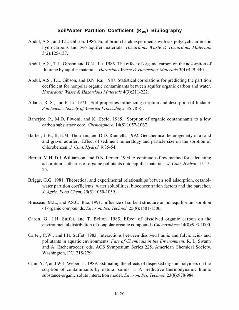
Soil/Water Partition Coefficient (Koc) Bibliography
Abdul, A.S., and T.L. Gibson. 1986. Equilibrium batch experiments with six polycyclic aromatichydrocarbons and two aquifer materials. Hazardous Waste & Hazardous Materials3(2):125-137.
Abdul, A.S., T.L. Gibson and D.N. Rai. 1986. The effect of organic carbon on the adsorption offluorene by aquifer materials. Hazardous Waste & Hazardous Materials 3(4):429-440.
Abdul, A.S., T.L. Gibson, and D.N. Rai. 1987. Statistical correlations for predicting the partitioncoefficient for nonpolar organic contaminants between aquifer organic carbon and water.Hazardous Waste & Hazardous Materials 4(3):211-222.
Adams, R. S., and P. Li. 1971. Soil properties influencing sorption and desorption of lindane.Soil Science Society of America Proceedings. 35:78-81.
Banerjee, P., M.D. Piwoni, and K. Ebeid. 1985. Sorption of organic contaminants to a lowcarbon subsurface core. Chemosphere. 14(8):1057-1067.
Barber, L.B., II, E.M. Thurman, and D.D. Runnells. 1992. Geochemical heterogeneity in a sandand gravel aquifer: Effect of sediment mineralogy and particle size on the sorption ofchlorobenzen. J. Cont. Hydrol. 9:35-54.
Barrett, M.H.,D.J. Williamson, and D.N. Lerner. 1994. A continuous flow method for calculatingadsorption isotherms of organic pollutants onto aquifer materials. J. Cont. Hydrol . 15:15-25.
Briggs, G.G. 1981. Theoretical and experimental relationships betwen soil adsorption, octanol-water partition coefficients, water solubilities, bioconcentration factors and the parachor.J. Agric. Food Chem. 29(5):1050-1059.
Brusseau, M.L., and P.S.C. Rao. 1991. Influence of sorbent structure on nonequilibrium sorptionof organic compounds. Environ. Sci. Technol. 25(8):1501-1506.
Caron, G., I.H. Suffet, and T. Belton. 1985. Effect of dissolved organic carbon on theenvironmental distribution of nonpolar organic compounds.Chemosphere.14(8):993-1000.
Carter, C.W., and I.H. Suffet. 1983. Interactions between disolved humic and fulvic acids andpollutants in aquatic environments. Fate of Chemicals in the Environment. R. L. Swannand A. Eschenroeder, eds. ACS Symposium Series 225. American Chemical Society,Washington, DC. 215-229.
Chin, Y.P, and W.J. Weber, Jr. 1989. Estimating the effects of dispersed organic polymers on thesorption of contaminants by natural solids. 1. A predictive thermodynamic humicsubstance-organic solute interaction model. Environ. Sci. Technol. 23(8):978-984.
K-20

Chiou, C.T., L.J. Peters, and V.H. Freed. 1979. A physical concept of soil-water equilibria fornonionic organic compounds. Science. 206:831-832.
Chiou, C.T., P.E. Porter, and D.W. Schmedding. 1983. Partition equilibria of nonionic organiccompounds between soil organic matter and water. Environ. Sci. Technol. 17(4):227-231.
Daniels, S. L., F. D. Hoerger, and R. J. Moolenar. 1985. Environmental exposure assessment:experience under the Toxics Substance Control Act. Environ. Toxicol. Chem. 4:107-117.
Di Toro, D.M. 1985. A particle interaction model of reversible organic chemical sorption.Chemosphere. 14(10):1503-1538.
Friesel, P., G. Milde, and B. Steiner. 1984. Interactions of halogenated hydrocarbons with soils.Fresenius Z. Anal. Chem. 319:160-164.
Garbarini, D.R., and L.W. Lion. 1986. Influence of the nature of soil organics on the sorptionof toluene and trichloroethylene. Environ. Sci. Technol. 20(12):1263-1269.
Gauthier, T.D., W.R. Seltz, and C.L. Grant. 1987. Effects of structural and compositionalvariations of dissolved humic materials on pyrene Koc values. Environ. Sci. Technol.21(3):243-248.
Gerstl, Z. 1990. Evaluating the Groundwater Pollution Hazard of Toxic Organics by MolecularConnectivity. Final Report. Institute of Soils and Water, The Volcani Center, Bet Dagan,Israel.
Gerstl, Z., and U. Mingelgrin. 1984. Sorption of organic substances by soils and sediments. J.Environ. Sci. Health B19(3):297-312.
Gledhill, W.E., R.G. Kaley, W.J. Adams, O. Hicks, P. R. Michael, V.W. Saeger, and G. A.LeBlanc. 1980. An environmental safety assessment of butyl benzyl phthalate. Environ.Sci. Technol. 14(3):301-305.
Grathwohl, P. 1990. Influence of organic matter from soils and sediments from various originson the sorption of some chlorinated aliphatic hydrocarbons: implications on Koc
correlations. Environ. Sci. Technol. 24(11):1687-1693.
Hassett, J.J., J.C. Means, W.L. Banwart, and S.G. Wood. 1980. Sorption Properties of Sedimentsand Energy-Related Pollutants. EPA 600/3-80-041. U.S. Environmental ProtectionAgency. Athens, GA.
Hodson, J., and N.A. Williams. 1988. The estimation of the adsorption coefficient (Koc) for soilsby high performance liquid chromatography. Chemosphere. 17(1):67-77.
K-21

Huggenberger, F.J. Letey, W.J. Farmer. 1972. Observed and calculated distribution of lindane insoil columns as influenced by water movement. Soil Sci. Soc. Am. Proc. 36:544-548.
Hutzler, N.J., J.C. Crittenden, J.L. Oravitz and P.A. Schaepe. 1983. Groundwater transport ofchlorinated organic compounds. In: American Chemical Society, Div. Environ. Chem.,186th National Meeting. 23:499-502.
Hutzler, N.J., J.C. Crittenden, and J. S. Gierke. 1986. Transport of organic compounds withsaturated groundwater flow: experimental results. Water Resources Res. 22(3):285-295.
Johnson-Logan, L.R., R.E. Broshears, and S.J. Klaine. 1992. Partitioning behavior and themobility of chlordane in groundwater. Environ. Sci. Technol. 26(11):2234-2239.
Jury, W.A., W.J. Farmer, and W.F. Spencer. 1984. Behavior assessment model for trace organicsin soil: II. Chemical classification and parameter sensitivity. J. Environ. Qual. 13(4):567-572.
Jury, W.A., D Russo, G.Streile, and H.E. Abd. 1990. Evaluation of volatilization by organicchemicals residing below the soil surface. Water Resources Res. 26(1):13-20.
Kan, A.T., and M.B.Tomson. 1990. Ground water transport of hydrophobic organic compoundsin the presence of dissolved organic matter. Environ. Toxicol. Chem. 9:253-263.
Karickhoff, S.W. 1981. Semi-empirical estimation of sorption of hydrophobic pollutants onnatural sediments and soils. Chemosphere. 10(8):833-846.
Karickhoff, S.W. 1982. Sorption kinetics of hydrophobic pollutants in natural sediments.Contaminants and Sediments. 2:193-205.
Karickhoff, S.W., D.S. Brown, and T.A. Scott. 1979. Sorption of hydrophobic pollutants onnatural sediments. Water Res. 13:241-248.
Karickhoff, S.W., and K.R.Morris. 1985a. Impact of tubificid oligochaetes on pollutant transportin bottom sediments. Environ. Sci. Tech. 19:51-56.
Karickhoff, S.W., and K.R. Morris. 1985b. Sorption dynamics of hydrophobic pollutants insediment suspensions. Environ. Toxicol. Chem. 4:469-479.
Kay, B.D., and D.E. Elrick. 1967. Adsorption and movement of lindane in soils. Soil Science.104:314.
Kishi, H., N. Kogure, and Y. Hashimoto. 1990. Contribution of soil constituents in adsorptioncoefficient of aromatic compounds, halogenated alicyclic and aromatic compounds to soil.Chemosphere. 21(7):867-876.
K-22

Koch, R. 1983. Molecular connectivity index for assessing ecotoxicological behaviour of organiccompounds. Toxicol. Environ. Chem. 6:87-96.
Landrum, P.F., S.R. Nihart, B.J. Eadie, and W.S. Gardner. 1984. Reverse-phase separationmethod for determining pollutant binding to aldrich humic acid and dissolved organiccarbon of natural waters. Environ. Sci. Technol. 18(3):187-192.
Lee, J.F., J.R. Crum, and S.A. Boyd. 1989. Enhances retention of organic contaminants by soilsexchanged with organic cations. Environ. Sci. Technol. 23(11):1365-1372.
Leistra, M. 1970. Distribution of 1,3-dichloropropene over the phases in soil. J.Agr. Food Chem.18(6):1124-1126.
Loch, J.P.G., H.J. Kool, P. Lagas, and J.H.A.M. Verheul. 1986. Removal and retention of volatilechlorinated hydrocarbons in the soils' unsaturated zone. In: Contaminated Soil. J.W.Assink and W.J. van der Brink, eds. Matinus Nijhoff Publishers, Dordrecht, Netherlands.63-77.
Lokke, H. 1984. Sorption of selected organic pollutants in Danish soils. Ecotoxicol. Environ.Safety 8:395-409.
Lord, K.A., G.G. Briggs, M.C. Neale, and R. Manlove. 1980. Uptake of pesticides from waterand soil by earthworms. Pest. Sci. 11:401-408.
Lotse, E.J., D.A. Graetz, G. Chesters, G.B. Lee, and L.W. Newland. 1968. Environ. Sci. Technol.2:353.
Mackay, D., W. Y. Shiu, and K. C. Ma. 1992. Illustrated Handbook of Physical-ChemicalProperties and Environmental Fate for Organic Chemicals. Volume I - MonoaromaticHydrocarbons, Chlorobenzenes, and PCB's. Lewis Publishers, Boca Raton, FL.
Mackay, D., W. Y. Shiu, and K. C. Ma. 1993. Illustrated Handbook of Physical-ChemicalProperties and Environmental Fate for Organic Chemicals. Volume III - Volatile OrganicChemicals. Lewis Publishers, Boca Raton, FL.
McCall, P.J., R.L. Swann, D.A. Laskowski, S.M. Unger, S.A. Vrona, and H.J. Dishburger. 1980.Estimation of chemical mobility in soil from liquid chromatographic retention times. Bull.Environ. Contam. Toxicol. 24:190-195.
McCall, P.J., R.L. Swann, D.A. Laskowski. 1983. Partition models for equilibrium distributionof chemicals in environmental compartments. In: Fate of Chemicals in the Environment.R. L. Swann and A. Eschenroeder, eds. ACS Symposium Series 225. American ChemicalSociety, Washington, DC. 105-123.
K-23

McCarthy, J.F., and B.D.Jimenez. 1985. Interactions between polycyclic aromatic hydrocarbonsand dissolved humic material: binding and dissociation. Environ. Sci. Technol.19(11):1072-1076.
Means, J.C., S.G. Wood, J.J. Hassett, and W.L. Banwart, 1980. Sorption of polynuclear aromatichydrocarbons by sediments and soils. Environ. Sci. Technol. 14(12):1524-1528.
Meylan, W., P.H. Howard, and R.S. Boethling. 1992. Molecular topology/fragment contributionmethod for predicting soil sorption coefficients. Environ. Sci. Technol., 26(8):1560-1567.
Miller, C.T., and W.J. Weber, Jr. 1986. Sorption of hydrophobic organic pollutants in saturatedsoil systems. J. Cont. Hydrol. 1(1/2):243-261.
Mills, A.C., and J.W. Biggar. 1969a. Adsorption of gamma-BHC from solutions on severalselected adsorbents. J. Agric. Food Chem. 17(3):604-608.
Mills, A.C., and J.W. Biggar. 1969b. Solubility-temperature effects on the adsorption of gamma-and beta-BHC from aqueous and hexane solutions by soil materials. Soil Sci. Soc. Amer.Proc. 33:210-216.
Moreale, A., and R. van Bladel. 1978. Adsorption et migration du lindane (1,2,3,4,5,6-hexachlorohexane) dans les sols. Parasitica. 34(4):233-255.
Paviostathis, S.G. , and K. Jaglal. 1991. Desorptive behavior of trichloroethylene in contaminatedsoil. Environ. Sci. Technol. 25(2):274-279.
Paviostathis, S.G., and G.N. Mathavan. 1992. Desorption kinetics of selected volatile organiccompounds from field contaminated soils. Environ. Sci. Technol. 26(3):532-538.
Pignatello, J.J. 1990. Slowly reversible sorption of aliphatic halocarbons in soils. I. formation ofresidual fractions. Environ. Toxicol. Chem. 9:1107-1115.
Pignatello, J.J. 1991. Desorption of tetrachloroethene and 1,2-dibromo-3-chloropropane fromaquifer sediments. Environ. Toxicol. Chem. 10:1399-1404.
Piwoni, M.D., and P. Banerjee. 1989. Sorption of volatile organic solvents from aqueous solutiononto subsurface solids. J. Contam. Hydrol. 4(2):163-179.
Podoll, R.T., K.C. Irwin, and H.J. Parish. 1989. Dynamic studies of naphthalene sorption on soilfrom aqueous solution. Chemosphere. 18(11/12):2399-2412.
Reinbold, K.A., J.J. Hassett, J.C. Means, and W.L. Banwart. 1979. Adsorption of Energy-RelatedOrganic Pollutants: A Literature Review. EPA 600/3-79-086. U.S. EnvironmentalProtection Agency. Washington, DC.
K-24

Rippen, G., M. Ilgenstein, W. Klopffer, and H.J. Poremski. 1982. Screening of the adsorptionbehavior of new chemicals: natural soils and model adsorbents. Ecotoxicol. Environ.Safety 6:236-245.
Roberts, P.V., P.L. McCarty, M. Reinhard, and J. Schreiner. 1980. Organic contaminant behaviorduring groundwater recharge. Water Poll. Control Fed. J. 52:161-172.
Rogers, R.D., J.C. McFarlane, and A.J. Cross. 1980. Adsorption and desorption of benzene intwo soils and montmorillonite clay. J. Am. Chem. Soc. 14(4):457-460.
Rogers, R.D., and J.C. McFarlane. 1981. Sorption of carbon tetrachloride, ethylene dibromide,and trichloroethylene on soil and clay. Environ. Monitoring and Assessment. 1:155-162.
Roy, W.R., I. G. Krapac, S. F. J. Chou, and R. A. Griffin. 1987. Batch-Type AdsorptionProcedures for Estimating Soil Attenuation of Chemicals. Draft Technical ResourceDocument. EPA/530-SW-87-006. U. S. Environmental Protection Agency. Office ofResearch and Development. Cincinnati, OH. NTIS PB87-146155.
Russell, D.J., and B. McDuffie. 1986. Chemodynamic properties of phthalate esters: partitioningand soil migration. Chemosphere. 15(8):1003-1021.
Rutherford, D.W., and C.T. Chiou. 1992. Effect of water saturation in soil organic matter on thepartition of organic compounds. Environ. Sci. Technol. 26:965-970.
Rutherford, D.W., C.T. Chiou, and D.E. Kile. 1992. Influence of soil organic matter compositionon the partition of organic compounds. Environ. Sci. Technol. 26:336-340.
Scheunert, I., E. Topp, A. Attar, and F. Korte. 1994. Uptake pathways of chlorobenzenes inplants and their correlation with n-octanol/water partition coefficients. Ecotoxicol.Environ. Safety. 27:90-104.
Schwarzenbach, R.P., and J. Westall. 1981. Transport of nonpolar organic compounds fromsurface water to groundwater. Laboratory sorption studies. Environ. Sci. Technol.15(11):1360-1367.
Schwille, F. 1988. Dense Chlorinated Solvents in Porous and Fractured Media. LewisPublishers, Chelsea, MI.
Seip, H.M., J. Alstad, G.E. Carlberg, K. Martinsen, and R. Skanne. 1986. Measurement ofmobility of organic compounds in soils. Sci. Total Environ. 50:87-101.
Sharom, M.S., J.R.W. Miles, C.R. Harris, and F.L. McEwen. 1980. Behaviour of 12 insecticidesin soil and aqueous suspensions of soil and sediment. Water Res. 14:1095-1100.
K-25
Smith, J.A., C.T. Chiou, J.A. Kammer, and D.E. Kile. 1990. Effect of soil moisture on sorptionof trichloroethene vapor to vadose-zone soil at Picatinny Arsenal, New Jersey. Environ.Sci. Technol. 24(5):676-698.
Smith, J.H., W.R. Mabey, N. Bohonos, B.R. Holt, S.S. Lee, T.-W. Chou, D.C. Bomberger, andT. Mill. 1978. Environmental Pathways of Selected Chemicals in Freshwater Systems.Part 2: Laboratory Studies. EPA-600/7-78-074. U.S. Environmental Protection Agency,Athens, GA.
Southworth, G.R., and J.L. Keller. 1986. Hydrophobic sorption of polar organics by low organiccarbon soils. Water, Air, and Soil Pollution. 28:239-248.
Spencer, W.F., and M.M. Cliath. 1970. Desorption of lindane from soil as related to vapordensity. Soil Sci. Soc. Am. Proc. 34:574-578.
Stauffer, T.B., and W.G. MacIntyre. 1986. Sorption of low-polarity organic compounds on oxideminerals and aquifer material. Environ. Toxicol. Chem. 5:949-955.
Szabo, G., S.L. Prosser, and R.A. Bulman. 1990a. Determination of the adsorption coefficient(Koc) of some aromatics for soil by RP-HPLC on two immobilized humic acid phases.Chemosphere. 21(6):777-788.
Szabo, G., S.L. Prosser, and R.A. Bulman. 1990b. Prediction of the adsorption coefficient (Koc)for soil by a chemically immobilized humic acid column using RP-HPLC. Chemosphere.21(6):729-739.
Vowles, P.D., and R.F.C. Mantoura. 1987. Sediment-water partition coefficients and HPLCretention factors of aromatic hydrocarbons. Chemosphere. 16(1):109-116.
Wahid, P.A., and N. Sethunathan. 1978. A simple method to study pesticide sorption in soils atshort time intervals. Soil Sci. 126(1):56-58.
Wahid, P.A., and N. Sethunathan. 1979. Sorption-desorption of α , β and γ isomers ofhexachlorocyclohexane in soils.J. Agric. Food Chem. 27(5):1050-1053
Wahid, P.A., and N. Sethunathan. 1980. Sorption-desorption of lindane by anaerobic and aerobicsoils. J. Agric. Food Chem. 28(3):623-625.
Wauchope, R.D., T.M. Buttler, A.G. Hornsby, P.W.M. Augustijn-Beckers, and J.P. Burt. 1992.The SRS/ARS/CES pesticide properties database for environmental decision-making. Rev.Environ. Contam. & Toxicol. 123:1-164.
Wilson, J.T., C.G. Enfield, W.J. Dunlap, R.L. Cosby, D.A. Foster, and L.B. Baskin. 1981.Transport and fate of selected organic pollutants in a sandy soil. J. Environ. Qual.10(4):501-506.
K-26

Wood, A.L., D.C.Bouchard, M.L. Brusseau, and P.S.C. Rao. 1990. Cosolvent effects on sorptionand mobility of organic contaminants in soils. Chemosphere. 21(4-5):575-587.
Woodburn, K.B., L.S. Lee, P. Suresh, C. Rao, and J.J. Delfino. 1989. Comparison of sorptionenergetics for hydrophobic organic chemicals by synthetic and natural sorbents frommethanol/water solvent mixtures. Environ. Sci. Technol. 23:407-413.
Wu, S., and P.M. Gschwend. 1986. Sorption kinetics of hydrophobic organic compounds tonatural sediments and soils. Environ. Sci. Technol. 20:717-725.
K-27

APPENDIX L
Koc Values for Ionizing Organicsas a Function of pH

Ap
pen
dix
L.
Ko
c V
alu
es f
or
Ion
izin
g O
rgan
ics
as a
Fu
nct
ion
of
pH
Ko
c,n
pHp
Ka
ΦK
oc,
iK
oc
log
Ko
c
324.
94.
180.
1600
0.5
5.5
0.74
325.
04.
180.
1315
0.5
4.6
0.67
325.
14.
180.
1073
0.5
3.9
0.59
325.
24.
180.
0872
0.5
3.2
0.51
325.
34.
180.
0705
0.5
2.7
0.43
325.
44.
180.
0568
0.5
2.3
0.36
325.
54.
180.
0457
0.5
1.9
0.29
325.
64.
180.
0366
0.5
1.7
0.22
325.
74.
180.
0293
0.5
1.4
0.15
325.
84.
180.
0234
0.5
1.2
0.09
325.
94.
180.
0187
0.5
1.1
0.04
326.
04.
180.
0149
0.5
1.0
-0.0
132
6.1
4.18
0.01
190.
50.
9-0
.06
326.
24.
180.
0095
0.5
0.8
-0.1
032
6.3
4.18
0.00
750.
50.
7-0
.13
326.
44.
180.
0060
0.5
0.7
-0.1
632
6.5
4.18
0.00
480.
50.
7-0
.19
326.
64.
180.
0038
0.5
0.6
-0.2
132
6.7
4.18
0.00
300.
50.
6-0
.23
326.
84.
180.
0024
0.5
0.6
-0.2
432
6.9
4.18
0.00
190.
50.
6-0
.25
327.
04.
180.
0015
0.5
0.5
-0.2
632
7.1
4.18
0.00
120.
50.
5-0
.27
327.
24.
180.
0010
0.5
0.5
-0.2
732
7.3
4.18
0.00
080.
50.
5-0
.28
327.
44.
180.
0006
0.5
0.5
-0.2
832
7.5
4.18
0.00
050.
50.
5-0
.29
327.
64.
180.
0004
0.5
0.5
-0.2
932
7.7
4.18
0.00
030.
50.
5-0
.29
327.
84.
180.
0002
0.5
0.5
-0.3
032
7.9
4.18
0.00
020.
50.
5-0
.30
328.
04.
180.
0002
0.5
0.5
-0.3
0
Ben
zoic
Aci
d
-0.4
-0.20.0
0.2
0.4
0.6
0.8
4.9
5.4
5.9
6.4
6.9
7.4
7.9
pH
log Koc
K-1

Ap
pen
dix
L.
Ko
c V
alu
es f
or
Ion
izin
g O
rgan
ics
as a
Fu
nct
ion
of
pH
Ko
c,n
pHp
Ka
ΦK
oc,
iK
oc
log
Ko
c
398
4.9
8.40
0.99
976
398
2.60
398
5.0
8.40
0.99
966
398
2.60
398
5.1
8.40
0.99
956
398
2.60
398
5.2
8.40
0.99
946
398
2.60
398
5.3
8.40
0.99
926
398
2.60
398
5.4
8.40
0.99
906
398
2.60
398
5.5
8.40
0.99
876
397
2.60
398
5.6
8.40
0.99
846
397
2.60
398
5.7
8.40
0.99
806
397
2.60
398
5.8
8.40
0.99
756
397
2.60
398
5.9
8.40
0.99
686
397
2.60
398
6.0
8.40
0.99
606
396
2.60
398
6.1
8.40
0.99
506
396
2.60
398
6.2
8.40
0.99
376
396
2.60
398
6.3
8.40
0.99
216
395
2.60
398
6.4
8.40
0.99
016
394
2.60
398
6.5
8.40
0.98
766
393
2.59
398
6.6
8.40
0.98
446
392
2.59
398
6.7
8.40
0.98
046
390
2.59
398
6.8
8.40
0.97
556
388
2.59
398
6.9
8.40
0.96
936
386
2.59
398
7.0
8.40
0.96
176
383
2.58
398
7.1
8.40
0.95
236
379
2.58
398
7.2
8.40
0.94
066
375
2.57
398
7.3
8.40
0.92
646
369
2.57
398
7.4
8.40
0.90
916
362
2.56
398
7.5
8.40
0.88
826
354
2.55
398
7.6
8.40
0.86
326
344
2.54
398
7.7
8.40
0.83
376
333
2.52
398
7.8
8.40
0.79
926
319
2.50
398
7.9
8.40
0.75
976
304
2.48
398
8.0
8.40
0.71
536
286
2.46
2-C
hlo
rop
hen
ol
2.44
2.46
2.48
2.50
2.52
2.54
2.56
2.58
2.60
4.9
5.4
5.9
6.4
6.9
7.4
7.9
pH
log Koc
K-2
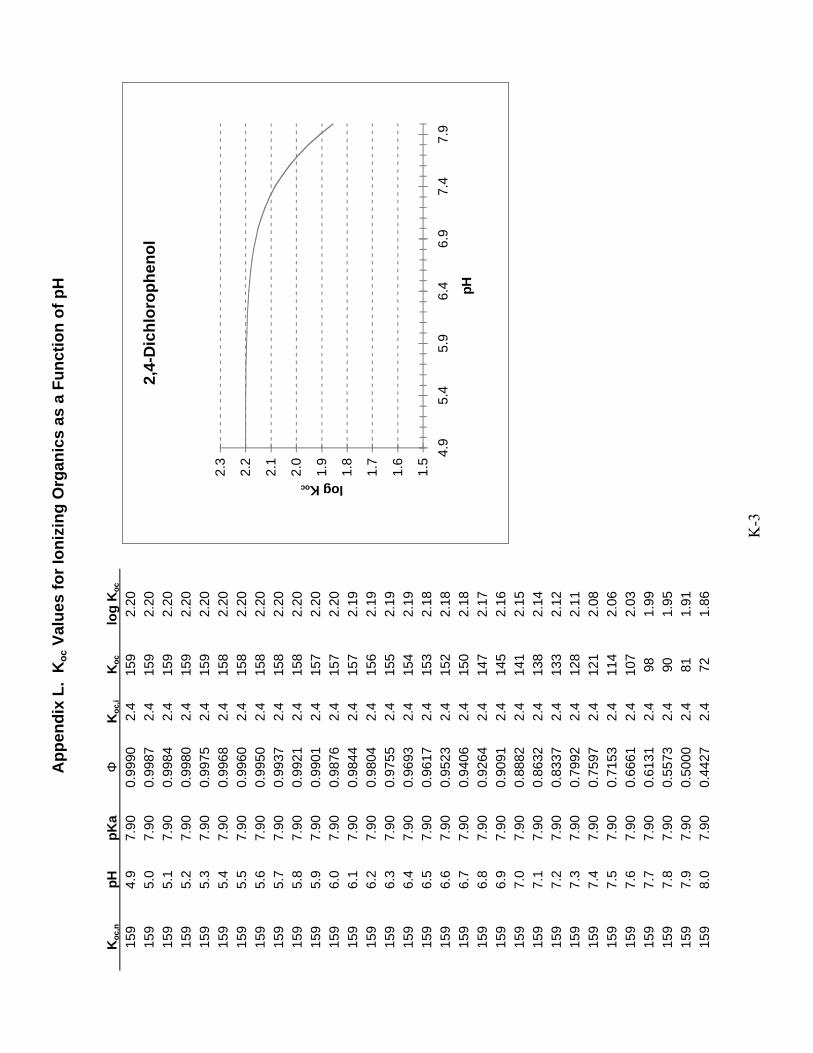
Ap
pen
dix
L.
Ko
c V
alu
es f
or
Ion
izin
g O
rgan
ics
as a
Fu
nct
ion
of
pH
Ko
c,n
pHp
Ka
ΦK
oc,
iK
oc
log
Ko
c
159
4.9
7.90
0.99
902.
415
92.
2015
95.
07.
900.
9987
2.4
159
2.20
159
5.1
7.90
0.99
842.
415
92.
2015
95.
27.
900.
9980
2.4
159
2.20
159
5.3
7.90
0.99
752.
415
92.
2015
95.
47.
900.
9968
2.4
158
2.20
159
5.5
7.90
0.99
602.
415
82.
2015
95.
67.
900.
9950
2.4
158
2.20
159
5.7
7.90
0.99
372.
415
82.
2015
95.
87.
900.
9921
2.4
158
2.20
159
5.9
7.90
0.99
012.
415
72.
2015
96.
07.
900.
9876
2.4
157
2.20
159
6.1
7.90
0.98
442.
415
72.
1915
96.
27.
900.
9804
2.4
156
2.19
159
6.3
7.90
0.97
552.
415
52.
1915
96.
47.
900.
9693
2.4
154
2.19
159
6.5
7.90
0.96
172.
415
32.
1815
96.
67.
900.
9523
2.4
152
2.18
159
6.7
7.90
0.94
062.
415
02.
1815
96.
87.
900.
9264
2.4
147
2.17
159
6.9
7.90
0.90
912.
414
52.
1615
97.
07.
900.
8882
2.4
141
2.15
159
7.1
7.90
0.86
322.
413
82.
1415
97.
27.
900.
8337
2.4
133
2.12
159
7.3
7.90
0.79
922.
412
82.
1115
97.
47.
900.
7597
2.4
121
2.08
159
7.5
7.90
0.71
532.
411
42.
0615
97.
67.
900.
6661
2.4
107
2.03
159
7.7
7.90
0.61
312.
498
1.99
159
7.8
7.90
0.55
732.
490
1.95
159
7.9
7.90
0.50
002.
481
1.91
159
8.0
7.90
0.44
272.
472
1.86
2,4-
Dic
hlo
rop
hen
ol
1.5
1.6
1.7
1.8
1.9
2.0
2.1
2.2
2.3
4.9
5.4
5.9
6.4
6.9
7.4
7.9
pH
log Koc
K-3

Ap
pen
dix
L.
Ko
c V
alu
es f
or
Ion
izin
g O
rgan
ics
as a
Fu
nct
ion
of
pH
Ko
c,n
pHp
Ka
ΦK
oc,
iK
oc
log
Ko
c
0.8
4.9
3.30
0.02
450.
010.
03-1
.53
0.8
5.0
3.30
0.01
960.
010.
03-1
.59
0.8
5.1
3.30
0.01
560.
010.
02-1
.65
0.8
5.2
3.30
0.01
240.
010.
02-1
.70
0.8
5.3
3.30
0.00
990.
010.
02-1
.75
0.8
5.4
3.30
0.00
790.
010.
02-1
.79
0.8
5.5
3.30
0.00
630.
010.
01-1
.82
0.8
5.6
3.30
0.00
500.
010.
01-1
.86
0.8
5.7
3.30
0.00
400.
010.
01-1
.88
0.8
5.8
3.30
0.00
320.
010.
01-1
.90
0.8
5.9
3.30
0.00
250.
010.
01-1
.92
0.8
6.0
3.30
0.00
200.
010.
01-1
.94
0.8
6.1
3.30
0.00
160.
010.
01-1
.95
0.8
6.2
3.30
0.00
130.
010.
01-1
.96
0.8
6.3
3.30
0.00
100.
010.
01-1
.97
0.8
6.4
3.30
0.00
080.
010.
01-1
.97
0.8
6.5
3.30
0.00
060.
010.
01-1
.98
0.8
6.6
3.30
0.00
050.
010.
01-1
.98
0.8
6.7
3.30
0.00
040.
010.
01-1
.99
0.8
6.8
3.30
0.00
030.
010.
01-1
.99
0.8
6.9
3.30
0.00
030.
010.
01-1
.99
0.8
7.0
3.30
0.00
020.
010.
01-1
.99
0.8
7.1
3.30
0.00
020.
010.
01-1
.99
0.8
7.2
3.30
0.00
010.
010.
01-2
.00
0.8
7.3
3.30
0.00
010.
010.
01-2
.00
0.8
7.4
3.30
0.00
010.
010.
01-2
.00
0.8
7.5
3.30
0.00
010.
010.
01-2
.00
0.8
7.6
3.30
0.00
010.
010.
01-2
.00
0.8
7.7
3.30
0.00
004
0.01
0.01
-2.0
00.
87.
83.
300.
0000
30.
010.
01-2
.00
0.8
7.9
3.30
0.00
003
0.01
0.01
-2.0
00.
88.
03.
300.
0000
20.
010.
01-2
.00
2,4-
Din
itro
ph
eno
l
-2.0
-1.9
-1.8
-1.7
-1.6
-1.5
4.9
5.4
5.9
6.4
6.9
7.4
7.9
pH
log Koc
K-4

Ap
pen
dix
L.
Ko
c V
alu
es f
or
Ion
izin
g O
rgan
ics
as a
Fu
nct
ion
of
pH
Ko
c,n
pHp
Ka
ΦK
oc,
iK
oc
log
Ko
c
1995
34.
94.
800.
4427
398
9055
3.96
1995
35.
04.
800.
3869
398
7964
3.90
1995
35.
14.
800.
3339
398
6927
3.84
1995
35.
24.
800.
2847
398
5965
3.78
1995
35.
34.
800.
2403
398
5097
3.71
1995
35.
44.
800.
2008
398
4325
3.64
1995
35.
54.
800.
1663
398
3650
3.56
1995
35.
64.
800.
1368
398
3073
3.49
1995
35.
74.
800.
1118
398
2584
3.41
1995
35.
84.
800.
0909
398
2176
3.34
1995
35.
94.
800.
0736
398
1837
3.26
1995
36.
04.
800.
0594
398
1560
3.19
1995
36.
14.
800.
0477
398
1331
3.12
1995
36.
24.
800.
0383
398
1147
3.06
1995
36.
34.
800.
0307
398
998
3.00
1995
36.
44.
800.
0245
398
877
2.94
1995
36.
54.
800.
0196
398
781
2.89
1995
36.
64.
800.
0156
398
703
2.85
1995
36.
74.
800.
0124
398
640
2.81
1995
36.
84.
800.
0099
398
592
2.77
1995
36.
94.
800.
0079
398
552
2.74
1995
37.
04.
800.
0063
398
521
2.72
1995
37.
14.
800.
0050
398
496
2.70
1995
37.
24.
800.
0040
398
476
2.68
1995
37.
34.
800.
0032
398
461
2.66
1995
37.
44.
800.
0025
398
447
2.65
1995
37.
54.
800.
0020
398
437
2.64
1995
37.
64.
800.
0016
398
429
2.63
1995
37.
74.
800.
0013
398
423
2.63
1995
37.
84.
800.
0010
398
418
2.62
1995
37.
94.
800.
0008
398
414
2.62
1995
38.
04.
800.
0006
398
410
2.61
Pen
tach
loro
ph
eno
l
2.00
2.25
2.50
2.75
3.00
3.25
3.50
3.75
4.00
4.9
5.4
5.9
6.4
6.9
7.4
7.9
pH
log Koc
K-5

Ap
pen
dix
L.
Ko
c V
alu
es f
or
Ion
izin
g O
rgan
ics
as a
Fu
nct
ion
of
pH
Ko
c,n
pHp
Ka
ΦK
oc,
iK
oc
log
Ko
c
1791
64.
96.
350.
9657
6717
304
4.24
1791
65.
06.
350.
9572
6717
152
4.23
1791
65.
16.
350.
9468
6716
966
4.23
1791
65.
26.
350.
9339
6716
736
4.22
1791
65.
36.
350.
9182
6716
456
4.22
1791
65.
46.
350.
8991
6716
115
4.21
1791
65.
56.
350.
8762
6715
706
4.20
1791
65.
66.
350.
8490
6715
221
4.18
1791
65.
76.
350.
8171
6714
651
4.17
1791
65.
86.
350.
7801
6713
991
4.15
1791
65.
96.
350.
7381
6713
241
4.12
1791
66.
06.
350.
6912
6712
404
4.09
1791
66.
16.
350.
6401
6711
492
4.06
1791
66.
26.
350.
5855
6710
518
4.02
1791
66.
36.
350.
5288
6795
063.
9817
916
6.4
6.35
0.47
1267
8477
3.93
1791
66.
56.
350.
4145
6774
653.
8717
916
6.6
6.35
0.35
9967
6491
3.81
1791
66.
76.
350.
3088
6755
793.
7517
916
6.8
6.35
0.26
1967
4742
3.68
1791
66.
96.
350.
2199
6739
923.
6017
916
7.0
6.35
0.18
2967
3332
3.52
1791
67.
16.
350.
1510
6727
623.
4417
916
7.2
6.35
0.12
3867
2277
3.36
1791
67.
36.
350.
1009
6718
683.
2717
916
7.4
6.35
0.08
1867
1527
3.18
1791
67.
56.
350.
0661
6712
473.
1017
916
7.6
6.35
0.05
3267
1017
3.01
1791
67.
76.
350.
0428
6783
12.
9217
916
7.8
6.35
0.03
4367
679
2.83
1791
67.
96.
350.
0274
6755
62.
7517
916
8.0
6.35
0.02
1967
458
2.66
2,3,
4,5-
Tet
rach
loro
ph
eno
l
2.6
3.0
3.4
3.8
4.2
4.6
4.9
5.4
5.9
6.4
6.9
7.4
7.9
pH
log Koc
K-6

Ap
pen
dix
L.
Ko
c V
alu
es f
or
Ion
izin
g O
rgan
ics
as a
Fu
nct
ion
of
pH
Ko
c,n
pHp
Ka
ΦK
oc,
iK
oc
log
Ko
c
6190
4.9
5.30
0.71
5393
4454
3.65
6190
5.0
5.30
0.66
6193
4154
3.62
6190
5.1
5.30
0.61
3193
3831
3.58
6190
5.2
5.30
0.55
7393
3491
3.54
6190
5.3
5.30
0.50
0093
3142
3.50
6190
5.4
5.30
0.44
2793
2792
3.45
6190
5.5
5.30
0.38
6993
2452
3.39
6190
5.6
5.30
0.33
3993
2129
3.33
6190
5.7
5.30
0.28
4793
1829
3.26
6190
5.8
5.30
0.24
0393
1558
3.19
6190
5.9
5.30
0.20
0893
1317
3.12
6190
6.0
5.30
0.16
6393
1107
3.04
6190
6.1
5.30
0.13
6893
927
2.97
6190
6.2
5.30
0.11
1893
775
2.89
6190
6.3
5.30
0.09
0993
647
2.81
6190
6.4
5.30
0.07
3693
542
2.73
6190
6.5
5.30
0.05
9493
455
2.66
6190
6.6
5.30
0.04
7793
384
2.58
6190
6.7
5.30
0.03
8393
327
2.51
6190
6.8
5.30
0.03
0793
280
2.45
6190
6.9
5.30
0.02
4593
242
2.38
6190
7.0
5.30
0.01
9693
213
2.33
6190
7.1
5.30
0.01
5693
188
2.27
6190
7.2
5.30
0.01
2493
169
2.23
6190
7.3
5.30
0.00
9993
153
2.19
6190
7.4
5.30
0.00
7993
141
2.15
6190
7.5
5.30
0.00
6393
131
2.12
6190
7.6
5.30
0.00
5093
123
2.09
6190
7.7
5.30
0.00
4093
117
2.07
6190
7.8
5.30
0.00
3293
113
2.05
6190
7.9
5.30
0.00
2593
108
2.03
6190
8.0
5.30
0.00
2093
105
2.02
2,3,
4,6-
Tet
rach
loro
ph
eno
l
1.8
2.2
2.6
3.0
3.4
3.8
4.9
5.4
5.9
6.4
6.9
7.4
7.9
pH
log Koc
K-7

Ap
pen
dix
L.
Ko
c V
alu
es f
or
Ion
izin
g O
rgan
ics
as a
Fu
nct
ion
of
pH
Ko
c,n
pHp
Ka
ΦK
oc,
iK
oc
log
Ko
c
2380
4.9
7.10
0.99
3736
2365
3.37
2380
5.0
7.10
0.99
2136
2361
3.37
2380
5.1
7.10
0.99
0136
2357
3.37
2380
5.2
7.10
0.98
7636
2351
3.37
2380
5.3
7.10
0.98
4436
2343
3.37
2380
5.4
7.10
0.98
0436
2334
3.37
2380
5.5
7.10
0.97
5536
2323
3.37
2380
5.6
7.10
0.96
9336
2308
3.36
2380
5.7
7.10
0.96
1736
2290
3.36
2380
5.8
7.10
0.95
2336
2268
3.36
2380
5.9
7.10
0.94
0636
2241
3.35
2380
6.0
7.10
0.92
6436
2207
3.34
2380
6.1
7.10
0.90
9136
2167
3.34
2380
6.2
7.10
0.88
8236
2118
3.33
2380
6.3
7.10
0.86
3236
2059
3.31
2380
6.4
7.10
0.83
3736
1990
3.30
2380
6.5
7.10
0.79
9236
1909
3.28
2380
6.6
7.10
0.75
9736
1817
3.26
2380
6.7
7.10
0.71
5336
1713
3.23
2380
6.8
7.10
0.66
6136
1597
3.20
2380
6.9
7.10
0.61
3136
1473
3.17
2380
7.0
7.10
0.55
7336
1342
3.13
2380
7.1
7.10
0.50
0036
1208
3.08
2380
7.2
7.10
0.44
2736
1074
3.03
2380
7.3
7.10
0.38
6936
943
2.97
2380
7.4
7.10
0.33
3936
819
2.91
2380
7.5
7.10
0.28
4736
703
2.85
2380
7.6
7.10
0.24
0336
599
2.78
2380
7.7
7.10
0.20
0836
507
2.70
2380
7.8
7.10
0.16
6336
426
2.63
2380
7.9
7.10
0.13
6836
357
2.55
2380
8.0
7.10
0.11
1836
298
2.47
2,4,
5-T
rich
loro
ph
eno
l
2.0
2.2
2.4
2.6
2.8
3.0
3.2
3.4
4.9
5.2
5.5
5.8
6.1
6.4
6.7
7.0
7.3
7.6
7.9
pH
log Koc
K-8

Ap
pen
dix
L.
Ko
c V
alu
es f
or
Ion
izin
g O
rgan
ics
as a
Fu
nct
ion
of
pH
Ko
c,n
pHp
Ka
ΦK
oc,
iK
oc
log
Ko
c
1070
4.9
6.40
0.96
9310
710
403.
0210
705.
06.
400.
9617
107
1033
3.01
1070
5.1
6.40
0.95
2310
710
243.
0110
705.
26.
400.
9406
107
1013
3.01
1070
5.3
6.40
0.92
6410
799
93.
0010
705.
46.
400.
9091
107
982
2.99
1070
5.5
6.40
0.88
8210
796
22.
9810
705.
66.
400.
8632
107
938
2.97
1070
5.7
6.40
0.83
3710
791
02.
9610
705.
86.
400.
7992
107
877
2.94
1070
5.9
6.40
0.75
9710
783
92.
9210
706.
06.
400.
7153
107
796
2.90
1070
6.1
6.40
0.66
6110
774
82.
8710
706.
26.
400.
6131
107
697
2.84
1070
6.3
6.40
0.55
7310
764
42.
8110
706.
46.
400.
5000
107
589
2.77
1070
6.5
6.40
0.44
2710
753
32.
7310
706.
66.
400.
3869
107
480
2.68
1070
6.7
6.40
0.33
3910
742
92.
6310
706.
86.
400.
2847
107
381
2.58
1070
6.9
6.40
0.24
0310
733
82.
5310
707.
06.
400.
2008
107
300
2.48
1070
7.1
6.40
0.16
6310
726
72.
4310
707.
26.
400.
1368
107
239
2.38
1070
7.3
6.40
0.11
1810
721
52.
3310
707.
46.
400.
0909
107
195
2.29
1070
7.5
6.40
0.07
3610
717
82.
2510
707.
66.
400.
0594
107
164
2.22
1070
7.7
6.40
0.04
7710
715
32.
1810
707.
86.
400.
0383
107
144
2.16
1070
7.9
6.40
0.03
0710
713
72.
1410
708.
06.
400.
0245
107
131
2.12
2,4,
6-T
rich
loro
ph
eno
l
2.00
2.20
2.40
2.60
2.80
3.00
3.20
4.9
5.4
5.9
6.4
6.9
7.4
7.9
pH
log Koc
K-9

APPENDIX M
Response to Peer-Review Comments on MINTEQA2Model Results

APPENDIX M
Response to Peer-Review Comments on MINTEQA2 Model Results
Peer review of the SSL MINTEQA2 model results identified several issues of concern, including
• The charge balance exceeds an acceptable margin of difference (5 percent) in most ofthe simulations. A variance in excess of 5 percent may indicate that the modelproblem is not correctly chemically poised and therefore the results may not bechemically meaningful.
• The model should not allow sulfate to adsorb to the iron oxide. Sulfate is a weaklyouter-sphere adsorbing species and by including the adsorption reaction, sulfate isremoved from the aqueous phase at pH values less than 7 and is prevented fromparticipating in precipitation reaction at these pH values.
• Modeled Kd values for barium and zinc could not be reproduced for all studied conditions.
The remainder of this Appendix addresses each of these issues.
Charge balance in the MINTEQA2 model runs
Although the charge imbalances (e.g., 6.8% at pH 8.0 and 54.9% at pH 4.9) are present especially athigh and low pH conditions, the conclusion that the charge imbalance makes the model results notchemically meaningful is not warranted.
MINTEQA2 uses two primary equations to solve chemical equilibrium problems: the mass actionequation (also called the mass law equation) and the mass balance equation. MINTEQA2 does not usethe charge balance equation to obtain the mathematical solution of the equilibrium problem. Thisdoes not mean that the charge balance equation has no meaning in MINTEQA2 calculations.
The reviewer's concern is understandable. It is logical that any chemical system whose charges arenot in balance must be incomplete or have erroneous concentrations for one or more components.However, the systems being modeled here are not "real" systems in the sense that they physicallyexist somewhere so that measurements can be made on them. Rather, they are generic,representative systems for ground water with variable (high, medium, low) concentrations of thoseparameters that most significantly impact Kd.
The modeled groundwater consists of national median concentrations of those major cations andanions that are most likely to impact the chemistry of the trace metal of interest by: (1) theircomplexation with the trace metal, (2) their competition with the trace metal for sorption sites,and/or (3) their effect on the ionic strength of the solution and thus, the activity coefficients of allspecies in solution including the trace metal. The settings of the three components of thisrepresentative system that have the greatest impact on the calculated Kd for various trace metals aresystematically varied. The three "master variable" components are pH, iron hydroxide sorption siteconcentration, and concentration of natural organic matter (particulate and dissolved).
M-1

No attempt was made to reconcile charge balances at the different settings of the three mastervariables. If reconciling charge balance had been attempted, it would have been accomplished byadjusting the concentrations of relatively inert anions and cations (e.g., NO3-, Na+) as needed tobalance the charge at equilibrium. It would be unwise to adjust the concentrations of more reactivecomponents (e.g., CO32-, Ca2+). To do so would be inconsistent with the initial assumption that thoseconstituents could be adequately represented by median concentrations observed in ground water andthat variability in the system could be captured by varying the three master components.
Table M-1 shows the result if the concentrations of the less reactive components NO3- and Na+ areadjusted in the high and low pH model runs so as to give a charge imbalance of <5% at equilibrium.The results shown pertain to the medium iron hydroxide and medium natural organic matter settingsfor zinc at the pH values listed. As shown in the table, the Kd values computed differ little fromthose presented in this report. The expected degree of error in the Kd values due to the manysimplifications and assumptions involved in generic modeling must surely exceed the variance due tocharge imbalance.
Table M-1. Kd values with and without counter ions (Na+ or NO3-) added to balance charge.
pH Kd1 (L/kg) No Counter Ion Added Kd
1 (L/kg) With Na+ or NO3- Added
4.9 1.61 1.51
8.0 16,161 16,135
1 Kd values shown correspond to the medium iron hydroxide, medium natural organic matter settings. Counter ionswere added to reduce charge imbalance to <5% at equilibrium.
Sulfate adsorption in MINTEQA2 model runs
The peer reviewer states that sulfate should not be allowed to adsorb to the iron oxide. The reviewerconcludes that by including the adsorption reactions "sulfate is removed from the aqueous phase atpH values less than 7 and is prevented from participating in precipitation reactions at these pHvalues".
The sulfate adsorption reactions on iron oxide included in the MINTEQA2 model runs were takenfrom a database of adsorption reactions that has been shown to give reliable results in predictingsulfate adsorption on pure phase iron oxide (Dzombak, 1986). The reviewer is correct in that freesulfate concentration is enhanced at low pH in runs without sulfate adsorption relative to runs withsulfate adsorption. However, for runs with low contaminant trace metal concentrations from whichthe SSL Kd's were taken, metal-sulfate precipitates do not form regardless of whether sulfateadsorption is included or not. Also, the Kd values over the entire range of trace metal concentrationsmodeled do not differ significantly when sulfate adsorption is included versus excluded.
Test runs were conducted on barium, zinc and cadmium at various settings of the three mastervariables (pH, natural organic matter (NOM) concentration, and iron oxide (FeOX) sorption siteconcentration). Table M-2 shows the Kd values for the lowest and highest trace metal concentrationfor model runs with and without sulfate adsorption. Results are shown for barium, zinc and cadmiumat the indicated settings of the master variables. Where results differ for the "with" and "without"
M-2

sulfate adsorption cases, it is most frequently due to the formation of aqueous complexes between thetrace metal and sulfate that compete with trace metal adsorption reactions, especially at low metalconcentrations.
Table M-2. Kd values calculated with and without sulfate adsorption reactions.
Metal (settings) Kd1 (L/kg) with SO4 adsorption Kd
1 (L/kg) without SO4 adsorption
Ba (MMH) 2.01 - 0.10 2.01 - 0.10
Ba (MMM) 1.37 - 0.04 1.37 - 0.04
Ba (LMM) 0.59 - 0.04 0.59 - 0.04
Ba (LLM) 0.12 - 0.01 0.12 - 0.01
Ba (LLL) 0.12 - 0.01 0.12 - 0.01
Zn (MMH) 1537 - 863 1478 - 830
Zn (LMM) 1.61 - 0.42 1.57 - 0.41
Zn (LML) 1.46 - 0.26 1.43 - 0.25
Cd (LMM) 0.94 - 0.01 0.91 - 0.01
1 Kd range shown corresponds to the lowest and highest trace metal concentrations. Master variable settings areindicated by a three letter code for each model run: the leftmost letter indicates pH, the middle letter represents theNOM concentration, and the rightmost letter indicates the concentration of FeOX adsorption sites (eg., HLMindicates high pH, low natural organic matter, medium and iron oxide site concentration).
Reproducing RTI results for barium and zinc
The peer reviewer had difficulty reproducing the Kd values computed for barium and zinc. Thereviewer included two sample input files for MINTEQA2 that had failed to produce results similar tothe SSL calculations.
The SSL results can be reproduced for all metals using the current version of MINTEQA2 (v3.11)distributed by EPA. As indicated in the 1994 Technical Background Document, a modified versionof this model was used to calculate SSL Kds. The current version can be used to calculate the sameresults by performing the following steps:
1) Edit the v3.11 component database file COMP.DBS to insert a component to representparticulate organic matter (POM). Use the 3-digit identifying number 251, a charge of -2.8, anda molar mass of zero.
2) Edit the v3.11 file THERMO.DBS to add the metal POM reactions shown in Appendix H of theRTI draft report. The file DATABASE.DOC included with MINTEQA2 v3.11 gives detailedinstructions for modifying the database file. After all reactions are added, del or rename thecurrent THERMO.UNF and TYPE6.UNF files and execute program UNFRMT (included withv3.11) to create new *.UNF files.
M-3

3) Observe that there were two modifications to v3.11 that make calculation of Kd in L/kg easier inthe version used by RTI. Since those modifications are not present in v3.11 itself, the user musttake care in computing Kd. The procedure is to first obtain the calculated concentration of themetal of interest (say, barium) bound with POM from PART 3 of the output file. If you have setthe solid precipitation flag to print a report each time a solid precipitates or dissolves, there willbe a series of PART 3 outputs each corresponding to a precipitation or dissolution event. Youmust be sure that the PART 3 output from which you obtain the metal-POM concentration isthe equilibrium output (i.e., it occurs prior to the PART 5 EQUILIBRATED MASSDISTRIBUTION with no intervening PROVISIONAL MASS DISTRIBUTION). After obtainingthe metal-POM concentration, locate the line corresponding to the trace metal of interest, saybarium in the PART 5 EQUILIBRATED MASS DISTRIBUTION section. Obtain the total sorbedconcentration value and to this value add the concentration of metal-POM species. This isnecessary because v3.11 recognizes only components with number 811 through 859 as sorptioncomponents. The metal-POM concentration will not have been added in the sorbed column. Itwill instead have been included in the dissolved column, so subtract the metal-POM concentrationfrom the dissolved total. Finally, to compute Kd, take the ratio of sorbed over dissolved (afterthe adjustment for metal-POM). The resulting Kd must be divided by 3.1778 kg/L (the mass ofsoil that one liter of solution is equilibrated with) to express the result in L/kg.
If the above three steps are followed, the v3.11 MINTEQA2 will give the same result as in the 1994Technical Background Document provided the data in the input file is correct. The two input filessent designed by the reviewer did not give correct results even when these steps were followed becauseof faulty values in the input file. The files supplied by the reviewer (SSLBA.INP and SSLZN.INP)were correct in all respects except two:
1) The site concentration for the POM component at the medium setting was entered as 1.930x10³
mg/L. This value was evidently obtained from the table on page 33 of the EPA report (US EPA,1992) after converting to mg/L. This is not the correct value for this the POM component. Thecorrect value is 9.31x10⁻⁴ mol/l and is found in the table on page 38 of EPA report.
2) The iron oxide adsorbent is represented by two site types (components 811 and 812). The highpopulation site has a lower affinity for the iron oxide surface for metals (expressed in a smallerlog K in the adsorption reactions involving metals). For a particular metal, say, zinc, it will benoted that there are two reactions in the database of 42 iron oxide adsorption reactions (FEW-DLM.DBS). This three-digit component number associated with the reaction having the smallerlog K of the two is the number to that must be used for the high population site. That is,component 812 should be entered at the higher site concentration and 811 at the lower siteconcentration. The set of site concentrations is given on page 44 of the EPA report. In thesample input files, component 811 was associated with the high site concentration and 812 withthe lower.
After correcting these two errors and observing the special requirements of using of v3.11 asindicated above, the Kd values obtained using MINTEQA2 v3.11 with the peer reviewer's files werevirtually identical to the SSL results.
M-4

References
Dzombak, D.A., 1986. Toward a Uniform Model for the Sorption of Inorganic Ions on HydrousOxides. Ph.D. Thesis, Massachusetts Institute of Technology, Cambridge, MA.
US EPA (Environmental Protection Agency), 1992. Background Document for Finite SourceMethodology for Wastes Containing Metals. HWEP-S0040. Office of Solid Waste,Washington, DC, 68 pages.
M-5