Sogachev Andrey Wind Energy Division, Risø National Laboratory for Sustainable Energy, DTU,...

Sogachev Andrey

Wind Energy Division, Risø National Laboratory for Sustainable Energy , DTU, Building 118, Box 49, DK-4000, Roskilde, Denmark, [email protected]

SCADIS (scalar distribution) model: overview

(Sogachev et al., 2002, 2004; Sogachev and Panferov, 2006; Sogachev et al., 2008, Sogachev 2009)

Basic equations:

momentum, heat,moisture,scalars (CO2, SO2, O3), turbulent kinetic energy (E)

One-and-a-half-order turbulence closurebased on equations of E and ε (dissipation rate) : ( E-l, E-ε.)

E-ω closure based on ω (ε/E) equation

Terrain-following coordinate system

Horizontal and vertical resolutions (depending on a specific problem)

SCADIS model: domain

q(t),T(t), C(t), V(t), U(t)

Clouds ( t )

T ( soil ), q ( soil ), FCO2

( soil ), V = 0 , U = 0

Q0

( t),

l o w e r b o u n d a r y c o n d i t i o n s

3 - 5 km

1 - 10 km

Upper boundary conditions


SCADIS model: physical processes in the model grid-cell

FCO2

E R H

G

y

f

x

f

¶

¶

¶

¶,

10 - 100 m

advection

y

f

x

f

,


Turbulence model: governing equations

.0

i

i

x

U

0

12 j ii i

j ijk j kj i j

u uU U PU U

t x x x

i

j

j

iijji x

U

x

UKEuu

3

2

E

iEijj P

x

EK

xx

EU

t

E

j

ijiE x

UuuP

iiuuE 21

l

EC

2343

EL P

CE

u 212

2 241 3 2 3Lu u u u u

iii uUU with

1 2jj i i

KU C P C

t x x x E

( , , )K f C E

( , , )l f C E

, ,El with

2

1 22 1

k

C C C

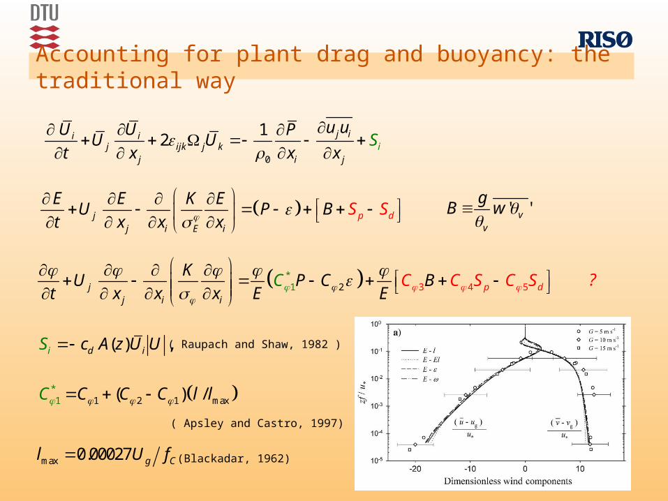
Accounting for plant drag and buoyancy: the traditional way

' 'vv

gB w

0

12 j ii i

j ijk j kj

ij i

u uU U PU U

x x xS

t

( Raupach and Shaw, 1982 )( ) ,i d iS c A z U U

?

j i

di

pjE

E E K EU P B

t x x xS S

*1 3 52 4 p dj

j i i

KU P C B

t x xC C S C S

EC

x E

1 2*1 1 max( ) /C C C C l l

( Apsley and Castro, 1997)

max 0.00027 g Cl U f (Blackadar, 1962)

Modelling of Askervein flow

Askervein Hill topographic map (brawn isolines) and dimensionless speed-up, ΔS estimated by SCADIS at z = 10 m above the ground (colored field). Figure 1 also shows the reference site (RS) (with ΔS = 0 ), the 210o wind direction in our simulations and the lines A, AA and B along which the measurements were made. Background of Figure 1 is taken from Castro et al., 2003.

Modelling of Askervein flow

Dimensionless speed-up, ΔS at z = 10 m above the ground along lines A (a) and AA (b). During measurements along line AA two different sets of instruments were used.

(a) (b)

Uncertainties: buoyancy

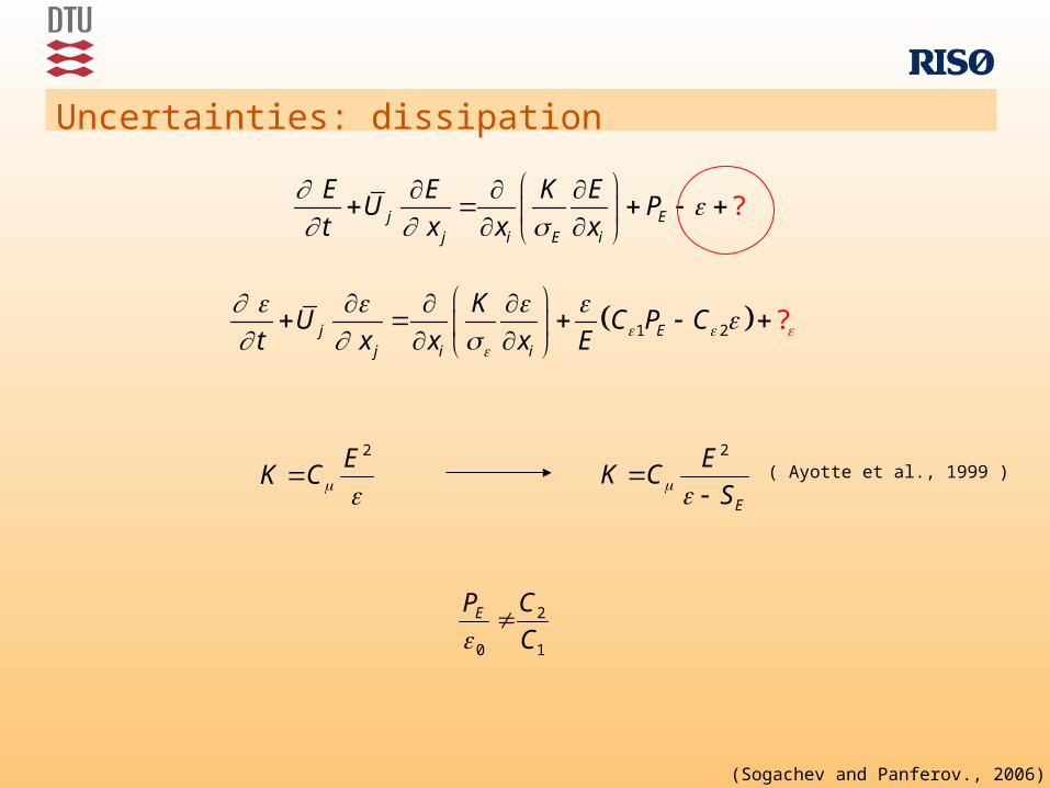
3 EB C BE

(Baumert and Peters, 2000)

?j Ej i E i

E E K EU P

t x x x

2ECK

ES

ECK

2

1 2 ?j Ej i i

KU C P C

t x x x E

1

2

0 C

CPE

( Ayotte et al., 1999 )

(Sogachev and Panferov., 2006)

Uncertainties: dissipation

Accounting for plant drag and buoyancy: the revised way

' 'vv

gB w

0

12 j ii i

j ijk j kj

ij i

u uU U PU U

x x xS

t

( Raupach and Shaw, 1982 )( ) ,i d iS c A z U U

1 2*1 1 max( ) /C C C C l l ( Apsley and Castro, 1997) max 0.00027 g Cl U f

0

dpS

jj i E i

S

E E K EU P B

t x x x

*1 2 1 2

*dj

j i i

KU P C C B

t x x x E EC C S

*15 2C CC *

13 2C CC 4 0C

1/ 212 ( )dd C cS A z U E (Sogachev and Panferov, 2006 )

(Blackadar, 1962)

(Sogachev 2009 )

dpS S (Seginer et al., 1976)

Accounting for plant drag and buoyancy: the revised way

... ?E

Pt

... ? ? ?E

Pt

*1 2? ?... P

t EC C

2*1

*21 ?

... PCt E

CC

C

E

2

2

1

2*

1

*

1

...

( )B d

P CCt E

C B a a SE

C

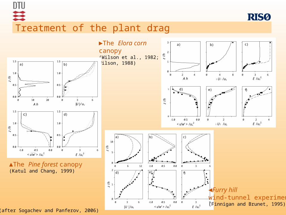
Treatment of the plant drag

a)

0 6 12

z / h

0

5

10

c)

0 3 6

b)

-1.0 -0.5 0.0

d)

| U | / u*

0 3 6

z / h

0

1

2e)

< u'w' > / u*2

-1.0 -0.5 0.0

f)

E / u*2

0 3 6

(after Sogachev and Panferov, 2006)

◄Furry hill wind-tunnel experiment(Finnigan and Brunet, 1995)

▲The Pine forest canopy (Katul and Chang, 1999)

►The Elora corn canopy (Wilson et al., 1982; Wilson, 1988)

a)

A h0 2 4

z / h

0

1

2

3

d)

< u'w' > / u*2

-1.0 -0.5 0.0

z / h

0

1

c)

E / u*2

0 3 6

b)

U / u*

0 4 8

e)

U / u*

0 2

f)

E / u*2

0 2 4

b)

|U| / u*

0 3 60.0

0.5

1.0

1.5

c)

< u'w' > / u*2

-1.0 -0.5 0.0

z / h

0.0

0.5

1.0

1.5d)

E / u*2

0 3 60.0

0.5

1.0

1.5

a)

A h

0 10 20

z / h

0.0

0.5

1.0

1.5

Treatment of the plant drag

(Sogachev and

Panferov, 2006)

4

2

6

x / h-10 0 10 20 30

z / h

0.0

0.5

1.0

1.5

2.0

2.5

3.0

1.0

0.5

1.5

1.0

0.5

x / h-10 0 10 20 30

10

5

x / h-10 0 10 20 30

U ( m s-1 ) l ( m ) E ( m2 s-2 )

a) E-l model

4

2

6

x / h-10 0 10 20 30

z / h

0.0

0.5

1.0

1.5

2.0

2.5

3.0

5

10

x / h

-10 0 10 20 30

1.0

1.00.5

1.0

0.5

0.5

x / h

-10 0 10 20 30

U ( m s-1 ) l ( m ) E ( m2 s-2 )

b) E- model

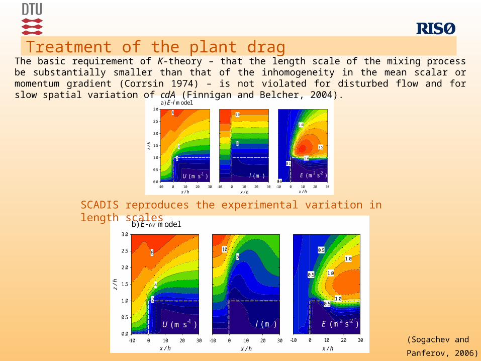
SCADIS reproduces the experimental variation in length scales

The basic requirement of K-theory – that the length scale of the mixing process be substantially smaller than that of the inhomogeneity in the mean scalar or momentum gradient (Corrsin 1974) – is not violated for disturbed flow and for slow spatial variation of cdA (Finnigan and Belcher, 2004).

Verification: low-roughness surface

Converse Prandtl number

1 4

1.35 /(1. 1.35Ri) for Ri 0

1.35 (1 15Ri ) for Ri 0

(Businger et al. 1971, Sogachev et al. 2002)

Wind speed ( m s-1 )Fig. 1 (a) ABL wind evolution and (b) surface characteristics: u* and Monin-Obukhov length, L, during fair weather over low-roughness land derived by E-ω model.

Uncertainties: Turbulent Prandtl number, Pr versus Ri

21Pr ( )z

UP B K Ri B

z

211 Pr ( )z Ri R

UP B K

zi

Verification: low-roughness surface

(Paulson, 1970)

0*

0

( ) lnzu z z

U zz L L

22ln 1 / 2 ln 1 / 2

2arctan / 2 0

5 0

X X

zz XLL

z z

L L

1 4

where 1 15z

XL

Fig. 2 (a) Wind evolutions and (b) wind profiles for different hours in the atmospheric surface layer during fair weather over low-roughness land derived by E-ω and analytical models.

Verification: forested surface

(Laakso et al., 2007)

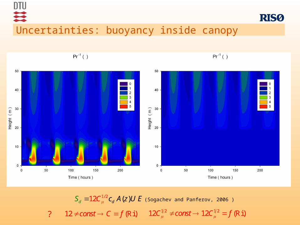
Uncertainties: buoyancy inside canopy


1/ 212 ( )dd cS A z U EC (Sogachev and Panferov, 2006 )

? 12 (Ri)const C f 1 2 1 212 12 (Ri)C const C f

Uncertainties: buoyancy inside canopyH =16 m, LAI = 1.38

(Christen and Novak, 2008)

ABL evolution

Energy budget above canopy layer

Ri in ABL

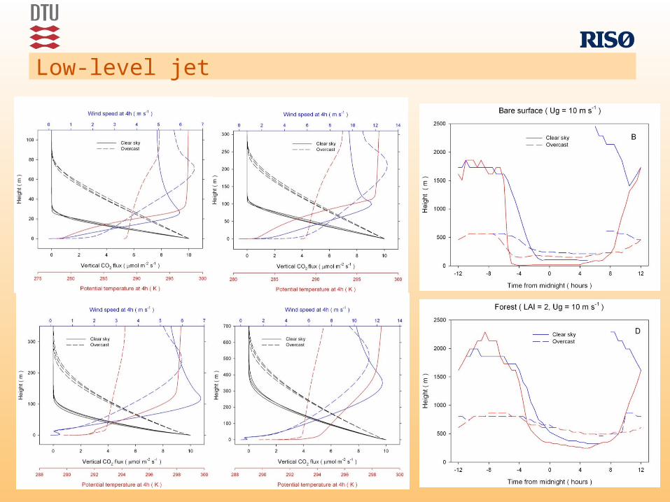
Low-level jet

Low-level jet effects on wind energy related variables

Summary

Much work remains to be done…

Sogachev Andrey Wind Energy Division, Risø National Laboratory for Sustainable Energy, DTU,...

Documents

Transcript of Sogachev Andrey Wind Energy Division, Risø National Laboratory for Sustainable Energy, DTU,...