Software Toolsfor

Discrete Mathematics

— User Manual —

Cordelia Hall and John O’Donnell

Last modified April 11, 2000

The Home Page for the book, from which you can obtain this document as well as thesoftware (Stfm.lhs) is available on the Web at

www.dcs.gla.ac.uk/~jtod/discrete-mathematics/

Copyright c© 2000 by Cordelia Hall and John O’Donnell

2

Contents

0 Getting Started 5Web Addresses . . . . . . . . . . . . . . . . . . . . . . . . . . . . . . . . . 5Instructor’s Guide . . . . . . . . . . . . . . . . . . . . . . . . . . . . . . . . 5Running Haskell 98 . . . . . . . . . . . . . . . . . . . . . . . . . . . . . . . 6

1 Introduction to Haskell 7

2 Propositional Logic 9Logical Operators . . . . . . . . . . . . . . . . . . . . . . . . . . . . . . . . . . . 9Using the Proof Checker . . . . . . . . . . . . . . . . . . . . . . . . . . . . . . . 10

Propositions . . . . . . . . . . . . . . . . . . . . . . . . . . . . . . . . . . . 10Theorems . . . . . . . . . . . . . . . . . . . . . . . . . . . . . . . . . . . . 11Inferences . . . . . . . . . . . . . . . . . . . . . . . . . . . . . . . . . . . . 12Assumptions . . . . . . . . . . . . . . . . . . . . . . . . . . . . . . . . . . . 12Inferences on the And operator . . . . . . . . . . . . . . . . . . . . . . . . 12Inferences on the Or operator . . . . . . . . . . . . . . . . . . . . . . . . . 13Inferences on Implication . . . . . . . . . . . . . . . . . . . . . . . . . . . . 14Inferences on Identity and False . . . . . . . . . . . . . . . . . . . . . . . . 14Represention of Proofs . . . . . . . . . . . . . . . . . . . . . . . . . . . . . 15

3 Predicate Logic 17

4 Set Theory 19

5 Recursion 23Recursion Over Lists . . . . . . . . . . . . . . . . . . . . . . . . . . . . . . . . . 23Higher Order Recursive Functions . . . . . . . . . . . . . . . . . . . . . . . . . . 24Recursion Over Trees . . . . . . . . . . . . . . . . . . . . . . . . . . . . . . . . . 24Peano Arithmetic . . . . . . . . . . . . . . . . . . . . . . . . . . . . . . . . . . . 26Data Recursion . . . . . . . . . . . . . . . . . . . . . . . . . . . . . . . . . . . . 28

6 Inductively Defined Sets 31

7 Induction 33

8 Relations 35

9 Functions 37

3

10 Digital Circuit Design 39

4

Chapter 0

Getting Started

Welcome to the User’s Manual for the Software Tools for Discrete Mathematics ! To usethis software, you should obtain:

• The book Discrete Mathematics Using a Computer, by Cordelia Hall and JohnO’Donnell. Published by Springer in January 2000 (£16.95, Softcover, 360 pages,ISBN 1-85233-089-9).

• The DMC Home Page on the Web, which contains general information as well asdirect links to the following items:

• The software Stdm.lhs, a source file in the Haskell 98 programming language.

• This manual, which is available on the web (in pdf format).

The software, this manual, and the web resources are intended to be used along with thebook. This isn’t a self-contained, standalone document!

Web Addresses

If you’re reading this document online, you can find everything you need by followingthe hyperlinks above. If you’re reading this on paper, however, you may need the WebURL addresses for (1) the DMC Home Page; (2 the software file Stfm.lhs; and (3) thismanual (pdf format):

www.dcs.gla.ac.uk/~jtod/discrete-mathematics/

www.dcs.gla.ac.uk/~jtod/discrete-mathematics/Stdm.lhs

www.dcs.gla.ac.uk/~jtod/discrete-mathematics/StdmMan.pdf

Instructor’s Guide

If you are teaching a course using these materials, you should also obtain access tothe Instructor’s Guide, whose URL is

www.dcs.gla.ac.uk/~jtod/discrete-mathematics/instructors-guide/

5

Running Haskell 98

The software tools are written in the standard language Haskell 98. Most of theimplementations of Haskell support experimental extensions to the language, as well asthe standard, so it’s important to tell the implementation to use Haskell 98.

The software uses the literate programming conventions of Haskell. This means thatevery line which begins with the > character will be compiled, but all other lines arecomments.

We recommend that you use the Haskell interpreter Hugs. To start Hugs in the Haskell98 mode, start it with the following command:

hugs +98

6

Chapter 1

Introduction to Haskell

Everything covered in this chapter is a feature of the Haskell 98 language, and Stdmdoesn’t contain any specific definitions relating to the chapter.

7

8

Chapter 2

Propositional Logic

Haskell uses the Bool type to represent propositional values. There are two constants oftype Bool, called True and False. (Be sure to make the first letter upper case!)

Logical Operators

Haskell provides several built-in logical operators using the Bool type. The (&&)

operator performs the logical and operation ∧:

(&&) :: Bool -> Bool -> Bool

False && False

==> False

False && True

==> False

True && False

==> False

True && True

==> True

The (||) operator performs the logical or operation ∨:

(||) :: Bool -> Bool -> Bool

False || False

==> False

False || True

==> True

True || False

==> True

True || True

==> True

Finally, the not function performs logical negation ¬:

not :: Bool -> Bool

not False

9

==> True

not True

==> False

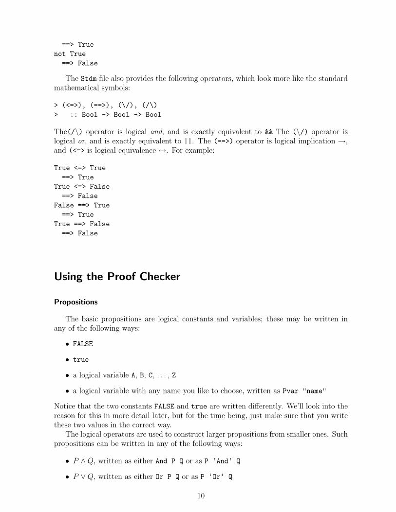
The Stdm file also provides the following operators, which look more like the standardmathematical symbols:

> (<=>), (==>), (\/), (/\)

> :: Bool -> Bool -> Bool

The(/\) operator is logical and, and is exactly equivalent to && The (\/) operator islogical or, and is exactly equivalent to ||. The (==>) operator is logical implication →,and (<=> is logical equivalence ↔. For example:

True <=> True

==> True

True <=> False

==> False

False ==> True

==> True

True ==> False

==> False

Using the Proof Checker

Propositions

The basic propositions are logical constants and variables; these may be written inany of the following ways:

• FALSE

• true

• a logical variable A, B, C, . . . , Z

• a logical variable with any name you like to choose, written as Pvar "name"

Notice that the two constants FALSE and true are written differently. We’ll look into thereason for this in more detail later, but for the time being, just make sure that you writethese two values in the correct way.

The logical operators are used to construct larger propositions from smaller ones. Suchpropositions can be written in any of the following ways:

• P ∧Q, written as either And P Q or as P ‘And‘ Q

• P ∨Q, written as either Or P Q or as P ‘Or‘ Q

10

Table 2.1: Examples of Proposition Representation

P P

P ∨Q Or P Q

P ‘Or‘ Q

P ∧Q And P Q

P ‘And‘ Q

(P ∧Q) ∨ (R ∧ S) Or (And P Q) (And R S)

((P ‘And‘Q) ‘Or‘ (R ‘And‘ S)

• P → Q, written as either Imp P Q or as P ‘Imp‘ Q

• ¬P , written as Not P

Parentheses are needed when the areguments to a logical operator are themselvesexpressions. For example, we can write P ∧Q as And P Q, without parentheses, but theexpression (P ∧Q) ∨R would be written as Or (And P Q) R, where the parentheses areessential. An alternative way to write this is (P ‘And‘ Q) ‘Or‘ R, but here again theparentheses are required to indicate the structure of the expression.

Theorems

A theorem in propositional logic always has a standard form: it says that a propositionp can be inferred from a set of assumptions a0, a1, . . . , ak−1. The mathematical notationfor this is

a0, a1, . . . , ak−1 ` p.

For example, the theorem

P,Q ` P ∧Q

has two assumptions P and Q, and the conclusion is P ∧Q. This statement means “giventhe assumptions P and Q, it is possible to infer the conclusion P ∧Q”. The number k ofassumptions may be 0; thus the theorem

` P → P

says that P → P can be proved without making any assumptions at all.To represent a theorem in Haskell, write Theorem, followed by a list of assumptions,

followed by the proposition which the theorem claims to hold. Thus the theorem

P,Q ` P ∧Q

would be represented as

Theorem [P,Q] (P ‘And‘ Q)

11

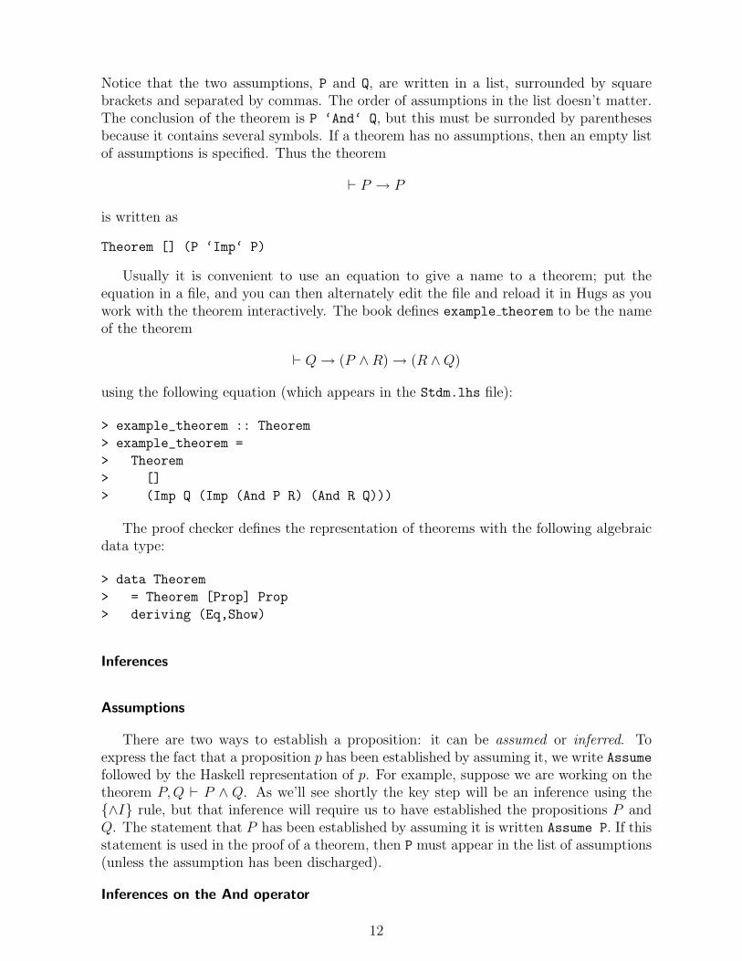
Notice that the two assumptions, P and Q, are written in a list, surrounded by squarebrackets and separated by commas. The order of assumptions in the list doesn’t matter.The conclusion of the theorem is P ‘And‘ Q, but this must be surronded by parenthesesbecause it contains several symbols. If a theorem has no assumptions, then an empty listof assumptions is specified. Thus the theorem

` P → P

is written as

Theorem [] (P ‘Imp‘ P)

Usually it is convenient to use an equation to give a name to a theorem; put theequation in a file, and you can then alternately edit the file and reload it in Hugs as youwork with the theorem interactively. The book defines example theorem to be the nameof the theorem

` Q→ (P ∧R)→ (R ∧Q)

using the following equation (which appears in the Stdm.lhs file):

> example_theorem :: Theorem

> example_theorem =

> Theorem

> []

> (Imp Q (Imp (And P R) (And R Q)))

The proof checker defines the representation of theorems with the following algebraicdata type:

> data Theorem

> = Theorem [Prop] Prop

> deriving (Eq,Show)

Inferences

Assumptions

There are two ways to establish a proposition: it can be assumed or inferred. Toexpress the fact that a proposition p has been established by assuming it, we write Assumefollowed by the Haskell representation of p. For example, suppose we are working on thetheorem P,Q ` P ∧ Q. As we’ll see shortly the key step will be an inference using the{∧I} rule, but that inference will require us to have established the propositions P andQ. The statement that P has been established by assuming it is written Assume P. If thisstatement is used in the proof of a theorem, then P must appear in the list of assumptions(unless the assumption has been discharged).

Inferences on the And operator

12

a b{∧I}

a ∧ ba ∧ b

{∧EL}a

a ∧ b{∧ER}

b

a{∨IL}

a ∨ bb{∨IR}

a ∨ ba ∨ b a ` c b ` c

{∨E}c

a ` b{→I}

a→ b

a a→ b{→E}

b

a{ID}

a

False{CTR}

a

¬a ` False{RAA}

a

Figure 2.1: Inference Rules of Propositional Logic.

The And-Introduction rule {∧I} says that if two propositions a and b have beenestablished, then their conjunction a ∧ b can be inferred.

a b{∧I}

a ∧ b

This inference is written in the form:

AndI (Proof,Proof) Prop

There are two And-Elimination rules, the “left” and “right” versions. In both casesthe rule’s assumption is that a conjunction of the form a ∧ b has been established. The“left” rule {∧EL} says that the leftmost part of the conjunction, a, can be inferred, whilethe “right” rule {∧ER} says that b may be inferred.

a ∧ b{∧EL}

a

a ∧ b{∧ER}

b

An inference using the {∧EL} rule is written as AndEL, followed by a proof of the con-junction a ∧ b, followed by the proposition a. The {∧ER} rule is similiar, using insteadthe AndER constructor.

Inferences on the Or operator

The Or-Introduction rule has two forms: the “left” form says that given a you caninfer a ∨ b for arbitrary b, and the “right” form says that you if you are given b then youcan infer a ∨ b.

13

a{∨IL}

a ∨ bb{∨IR}

a ∨ b

a ∨ b a ` c b ` c{∨E}

c

Inferences on Implication

a ` b{→I}

a→ b

a a→ b{→E}

b

Inferences on Identity and False

a{ID}

a

False{CTR}

a

¬a ` False{RAA}

a

The Proof Checker uses the following algebraic data type to represent inferences andproofs:

> data Proof

> = Assume Prop

> | AndI (Proof,Proof) Prop

> | AndEL Proof Prop

> | AndER Proof Prop

> | OrI1 Proof Prop

> | OrI2 Proof Prop

> | OrE (Proof,Proof,Proof) Prop

> | NotE (Proof,Proof) Prop

> | ImpI Proof Prop

> | ImpE (Proof,Proof) Prop

> deriving (Eq,Show)

14

Represention of Proofs

> proof1 =

> ImpI

> (ImpI

> (AndI

> ((AndER

> (Assume (And P R))

> R),

> Assume Q)

> (And R Q))

> (Imp (And P R) (And R Q)))

> (Imp Q (Imp (And P R) (And R Q)))

Valid proofs using And Introduction

Theorem 1. q, r ` q ∧ r

proof1 = AndI (Assume Q, Assume R) (And Q R)

Invalid proofs using And Introduction.

> p2 = -- q,r |- q&s

> AndI (Assume (Pvar "q"), Assume (Pvar "r"))

> (And (Pvar "q") (Pvar "s"))

Valid proofs using And Elimination (1)

> p3 = -- p&q |- p

> AndEL (Assume (And P Q)) P

> p4 = -- (P|Q)&R |- (P|Q)

> AndEL (Assume (And (Or P Q) R)) (Or P Q)

Invalid proofs using And Elimination (1)

> p5 = -- p&q |- p

> AndEL (Assume (Or P Q)) P

> p6 = -- p&q |- p

> AndEL (Assume (And P Q)) Q

> p7 = -- P&Q |- R

> AndEL (Assume (And P Q)) R

Valid proofs with Imp Introduction

> p81 = -- P,Q |- P&Q

> AndI (Assume P, Assume Q)

> (And P Q)

15

> p82 = -- Q |- (P => P&Q)

> ImpI (AndI (Assume P, Assume Q)

> (And P Q))

> (Imp P (And P Q))

> p83 = -- |- Q => (P => (P&Q))

> ImpI (ImpI (AndI (Assume P, Assume Q)

> (And P Q))

> (Imp P (And P Q)))

> (Imp Q (Imp P (And P Q)))

Valid proofs with Imp Elimination

> p9 = ImpE (Assume P, Assume (Imp P Q))

> Q

Here is the theorem and proofs that are used in the book; run them like this:

check_proof example_theorem proof1 (should be valid)

check_proof example_theorem proof2 (should give error message)

> example_theorem :: Theorem

> example_theorem =

> Theorem

> []

> (Imp Q (Imp (And P R) (And R Q)))

> proof1 =

> ImpI

> (ImpI

> (AndI

> ((AndER

> (Assume (And P R))

> R),

> Assume Q)

> (And R Q))

> (Imp (And P R) (And R Q)))

> (Imp Q (Imp (And P R) (And R Q)))

The following proof is incorrect proof, because QR was inferred where RQ was needed.

> proof2 =

> ImpI

> (ImpI

> (AndI

> (Assume Q,

> (AndER

> (Assume (And P R))

> R))

> (And R Q))

> (Imp (And P R) (And R Q)))

> (Imp Q (Imp (And P R) (And R Q)))

16

Chapter 3

Predicate Logic

Soon there will be more about this!

> forall :: [Int] -> (Int -> Bool) -> Bool

> exists :: [Int] -> (Int -> Bool) -> Bool

17

18

Chapter 4

Set Theory

A set will be represented as a list:

> type Set a = [a]

The subset function takes two sets as arguments, and returns True if the first is asubset of the second. (Note: the function does not reject non-sets.)

> subset :: (Eq a, Show a) => Set a -> Set a -> Bool

subset [4,3] [1,2,3,4,5]

==> True

subset [9,3] [1,2,3,4,5]

==> False

subset [1,2,3,4,5] [1,2,3,4,5]

==> True

subset [] []

==> True

The properSubset function implements ⊂; it is just like subset except that it returnsFalse if the first argument is equal to the second. (Note that properSubset does not rejectnon-sets.)

> properSubset :: (Eq a, Show a) => Set a -> Set a -> Bool

properSubset [4,3] [1,2,3,4,5]

==> True

properSubset [9,3] [1,2,3,4,5]

==> False

properSubset [1,2,3,4,5] [1,2,3,4,5]

==> False *** DIFFERENT FROM subset ***

properSubset [] []

==> True

The setEq function determines whether the two arguments represent the same set.They are equal if they contain the same elements, regardless of the order.

19

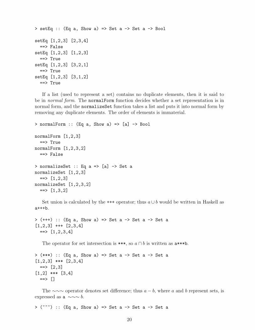
> setEq :: (Eq a, Show a) => Set a -> Set a -> Bool

setEq [1,2,3] [2,3,4]

==> False

setEq [1,2,3] [1,2,3]

==> True

setEq [1,2,3] [3,2,1]

==> True

setEq [1,2,3] [3,1,2]

==> True

If a list (used to represent a set) contains no duplicate elements, then it is said tobe in normal form. The normalForm function decides whether a set representation is innormal form, and the normalizeSet function takes a list and puts it into normal form byremoving any duplicate elements. The order of elements is immaterial.

> normalForm :: (Eq a, Show a) => [a] -> Bool

normalForm [1,2,3]

==> True

normalForm [1,2,3,2]

==> False

> normalizeSet :: Eq a => [a] -> Set a

normalizeSet [1,2,3]

==> [1,2,3]

normalizeSet [1,2,3,2]

==> [1,3,2]

Set union is calculated by the +++ operator; thus a∪ b would be written in Haskell asa+++b.

> (+++) :: (Eq a, Show a) => Set a -> Set a -> Set a

[1,2,3] +++ [2,3,4]

==> [1,2,3,4]

The operator for set intersection is ***, so a ∩ b is written as a***b.

> (***) :: (Eq a, Show a) => Set a -> Set a -> Set a

[1,2,3] *** [2,3,4]

==> [2,3]

[1,2] *** [3,4]

==> []

The ∼∼∼ operator denotes set difference; thus a− b, where a and b represent sets, isexpressed as a ∼∼∼ b.

> (~~~) :: (Eq a, Show a) => Set a -> Set a -> Set a

20

The !!! operator is used to calculate the complement of a set a with respect to auniverse u; this is expressed as u!!!a, and the value is equal to u ∼∼∼ s. If you’redoing many calculations with the same universe u, you can define a specific complementfunction specialised to that universe as compl = (u!!!).

> (!!!) :: (Eq a, Show a) => Set a -> Set a -> Set a

[2,4] !!! [1..5]

[1..5] !!! [2,4]

==> [1,3,5]

The powerset function returns the set of all subsets of its argument. If a set containsk elements, then its powerset will contain 2k elements.

> powerset :: (Eq a, Show a) => Set a -> Set (Set a)

powerset ([] :: [Int])

==> []

powerset [1]

==>[[1],[]]

powerset [1,2,3]

==> [[1,2,3],[1,2],[1,3],[1],[2,3],[2],[3],[]]

A minor point: in the first example above, where we take the powerset of the empty set, wedeclare the type of [] explicitly. This doesn’t have anything to do with the mathematics;it’s just a way of telling the Haskell typechecker what set type we are using.

The crossproduct function computes the set a × b, consisting of the set of all pairswhere the first element belongs to a and the second element belongs to b. That is,

a× b = {(x, y) | x ∈ a ∧ y ∈ b}.

> crossproduct

> :: (Eq a, Show a, Eq b, Show b)

> => Set a -> Set b -> Set (a,b)

crossproduct [1,2] [7,8,9]

==> [(1,7),(1,8),(1,9),(2,7),(2,8),(2,9)]

21

22

Chapter 5

Recursion

The factorial function is a typical example of a recursive definition. It has two equations;one for the base case 0, and one for the recursive case n+ 1.

> factorial :: Integer -> Integer

> factorial 0 = 1

> factorial (n+1) = (n+1) * factorial n

The first of these examples just uses the first equation, factorial 0 = 1; the othersrequire one or more applications of the second equation. In all cases, the evaluation stopswith the base case (the first equation).

factorial 0

==> 1

factorial 1

==> 1

factorial 5

==> 120

Recursion Over Lists

Here is the quicksort algorithm as presented in the book:

> quicksort :: Ord a => [a] -> [a]

> quicksort [] = []

> quicksort (splitter:xs) =

> quicksort [y | y <- xs, y<=splitter]

> ++ [splitter]

> ++ quicksort [y | y <- xs, y>splitter]

The following examples test quicksort on several input lists, but it is clear that testingcan never establish the correctness of the function; there are simply too many possibleinputs to try them all. We would need to prove its correctness mathematically, usinginduction.

23

quicksort [3,5,4]

==> [3,4,5]

quicksort [5,2,9,3,1,6,0,4,8,7]

==> [0,1,2,3,4,5,6,7,8,9]

quicksort ["bat","ant","mouse","dog"]

==> ["ant","bat","dog","mouse"]

Notice that quicksort is not restricted to sorting lists of numbers; the last exampleuses it to sort a list of strings. As the type says, quicksort can handle lists of any typea as long as a is in the Ord class (that is, the order operations can be applied to values oftype a). Compare this with what you have to do in conventional programming languages!

The book gives firsts as another example of recursion (here it’s called firsts1.However, the recursion pattern of firsts1 is expressed exactly by the map function, andit’s better programming style to use map directly, as in the alternative definition firsts2.

> firsts1, firsts2 :: [(a,b)] -> [a]

> firsts1 [] = []

> firsts1 ((a,b):ps) = a : firsts1 ps

> firsts2 xs = map fst xs

firsts1 [("cat",4), ("dog",8), ("mouse",2)]

==> ["cat","dog","mouse"]

firsts2 [("cat",4), ("dog",8), ("mouse",2)]

==> ["cat","dog","mouse"]

Higher Order Recursive Functions

Recursion Over Trees

There is really just one sensible way to define lists, so Haskell provides lists are a pre-defined type with a rich family of functions and operators. In contrast, there are manyways to define trees, and it isn’t reasonable to try to include them all in the standardlibraries. Consequently you need to define your own tree types when programming. Hereis the version of trees used in the book:

> data Tree a

> = Tip

> | Node a (Tree a) (Tree a)

> deriving Show

The following definition gives the names t1 and t2 to a couple of specific trees, whichwill be used in several of the following examples. Try evaluating t1 and t2 interactively.

24

> t1, t2 :: Tree Int

> t1 = Node 6 Tip Tip

> t2 = Node 5

> (Node 3 Tip Tip)

> (Node 8 (Node 6 Tip Tip) (Node 12 Tip Tip))

This function is a typical recursion over trees; it counts the number of Node con-structors in a tree. Notice that there is a base case and a recursion case, just as for listfunctions, but here the recursion case must call nodeCount twice, since there are twosubtrees under a Node.

> nodeCount :: Tree a -> Int

> nodeCount Tip = 0

> nodeCount (Node x t1 t2) = 1 + nodeCount t1 + nodeCount t2

nodeCount t1

==> 1

nodeCount t2

==> 5

The reflect function is a particularly elegant example of recursion.

> reflect :: Tree a -> Tree a

> reflect Tip = Tip

> reflect (Node a t1 t2) = Node a (reflect t2) (reflect t1)

reflect t1

==> Node 6 Tip Tip

reflect t2

==> Node 5 (Node 8 (Node 12 Tip Tip)

(Node 6 Tip Tip))

(Node 3 Tip Tip)

For any data structure we can define a map operation that applies some function f toevery element of the structure. Here is the mapTree function, which applies f :: a ->

b to every element in a Tree:

> mapTree :: (a->b) -> Tree a -> Tree b

> mapTree f Tip = Tip

> mapTree f (Node a t1 t2) =

> Node (f a) (mapTree f t1) (mapTree f t2)

mapTree (*10) t1

==> Node 60 Tip Tip

mapTree (*10) t2

==> Node 50 (Node 30 Tip Tip)

(Node 80 (Node 60 Tip Tip)

(Node 120 Tip Tip))

25

This tree stores a pair of type (Int,Int) in every Node, rather than just a singletonvalue. This gives us a little database.

> tree :: Tree (Int,Int)

> tree =

> Node (5,10)

> (Node (3,6) (Node (1,1) Tip Tip)

> (Node (4,8) Tip Tip))

> (Node (7,14) (Node (6,12) Tip Tip)

> (Node (8,16) Tip Tip))

The find function looks up a number in the database; if that number is found in thefirst element of a pair, then the second element is returned.

> find :: Int -> Tree (Int,a) -> Maybe a

> find n Tip = Nothing

> find n (Node (m,d) t1 t2) =

> if n==m then Just d

> else if n<m then find n t1

> else find n t2

find 6 tree

==> Just 12

find 7 tree

==> Just 14

find 20 tree

==> Nothing

Peano Arithmetic

Peano represents natural numbers; that is, the non-negative integers.

> data Peano = Zero | Succ Peano deriving Show

The following definitions will be used soon in several examples. Try evaluating theminteractively. Notice that that the Peano representation of k always contains exactly koccurrences of Succ.

> one = Succ Zero

> two = Succ one

> three = Succ two

> four = Succ three

> five = Succ four

> six = Succ five

The decrement function can be defined simply by pattern matching:

26

> decrement :: Peano -> Peano

> decrement Zero = Zero

> decrement (Succ a) = a

As an example, notice that decrement six produces the represenation of five.

five ==> Succ (Succ (Succ (Succ (Succ Zero))))

decrement six ==> Succ (Succ (Succ (Succ (Succ Zero))))

Most operations in Peano arithmetic must be defined using recursion; addition is atypical example:

> add :: Peano -> Peano -> Peano

> add Zero b = b

> add (Succ a) b = Succ (add a b)

add two three ==> Succ (Succ (Succ (Succ (Succ Zero))))

And here is subtraction:

> sub :: Peano -> Peano -> Peano

> sub a Zero = a

> sub Zero b = Zero

> sub (Succ a) (Succ b) = sub a b

sub six four

==> Succ (Succ Zero)

sub five one

==> Succ (Succ (Succ (Succ Zero)))

Testing for equality is similar. Notice that we don’t use the built-in Haskell (==)operator; instead we use recursion.

> equals :: Peano -> Peano -> Bool

> equals Zero Zero = True

> equals Zero b = False

> equals a Zero = False

> equals (Succ a) (Succ b) = equals a b

equals two three

==> False

equals four four

==> True

equals (add one two) (sub six three)

==> True

equals (sub four two) (add two three)

==> False

As one last example, here is the lt function, which computes the (<) relation:

27

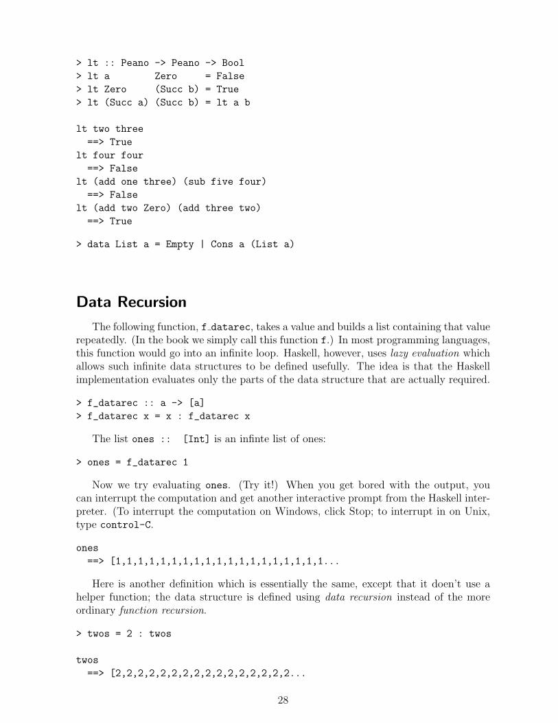
> lt :: Peano -> Peano -> Bool

> lt a Zero = False

> lt Zero (Succ b) = True

> lt (Succ a) (Succ b) = lt a b

lt two three

==> True

lt four four

==> False

lt (add one three) (sub five four)

==> False

lt (add two Zero) (add three two)

==> True

> data List a = Empty | Cons a (List a)

Data Recursion

The following function, f datarec, takes a value and builds a list containing that valuerepeatedly. (In the book we simply call this function f.) In most programming languages,this function would go into an infinite loop. Haskell, however, uses lazy evaluation whichallows such infinite data structures to be defined usefully. The idea is that the Haskellimplementation evaluates only the parts of the data structure that are actually required.

> f_datarec :: a -> [a]

> f_datarec x = x : f_datarec x

The list ones :: [Int] is an infinte list of ones:

> ones = f_datarec 1

Now we try evaluating ones. (Try it!) When you get bored with the output, youcan interrupt the computation and get another interactive prompt from the Haskell inter-preter. (To interrupt the computation on Windows, click Stop; to interrupt in on Unix,type control-C.

ones

==> [1,1,1,1,1,1,1,1,1,1,1,1,1,1,1,1,1,1,1...

Here is another definition which is essentially the same, except that it doen’t use ahelper function; the data structure is defined using data recursion instead of the moreordinary function recursion.

> twos = 2 : twos

twos

==> [2,2,2,2,2,2,2,2,2,2,2,2,2,2,2,2...

28

Any kind of circular data structure can be defined in a similar way:

> object = let a = 1:b

> b = 2:c

> c = [3] ++ a

> in a

object

==> [1,2,3,1,2,3,1,2,3,1,2,3,1,2,3,1,2,3...

29

30

Chapter 6

Inductively Defined Sets

31

32

Chapter 7

Induction

33

34

Chapter 8

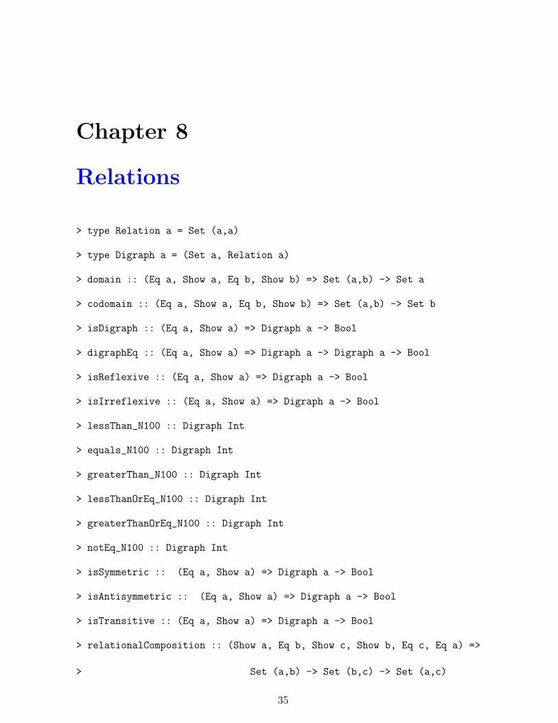
Relations

> type Relation a = Set (a,a)

> type Digraph a = (Set a, Relation a)

> domain :: (Eq a, Show a, Eq b, Show b) => Set (a,b) -> Set a

> codomain :: (Eq a, Show a, Eq b, Show b) => Set (a,b) -> Set b

> isDigraph :: (Eq a, Show a) => Digraph a -> Bool

> digraphEq :: (Eq a, Show a) => Digraph a -> Digraph a -> Bool

> isReflexive :: (Eq a, Show a) => Digraph a -> Bool

> isIrreflexive :: (Eq a, Show a) => Digraph a -> Bool

> lessThan_N100 :: Digraph Int

> equals_N100 :: Digraph Int

> greaterThan_N100 :: Digraph Int

> lessThanOrEq_N100 :: Digraph Int

> greaterThanOrEq_N100 :: Digraph Int

> notEq_N100 :: Digraph Int

> isSymmetric :: (Eq a, Show a) => Digraph a -> Bool

> isAntisymmetric :: (Eq a, Show a) => Digraph a -> Bool

> isTransitive :: (Eq a, Show a) => Digraph a -> Bool

> relationalComposition :: (Show a, Eq b, Show c, Show b, Eq c, Eq a) =>

> Set (a,b) -> Set (b,c) -> Set (a,c)

35

> equalityRelation :: (Eq a, Show a) => Set a -> Relation a

> relationalPower :: (Eq a, Show a) => Digraph a -> Int -> Relation a

> reflexiveClosure :: (Eq a, Show a) => Digraph a -> Digraph a

> inverse :: Set (a,b) -> Set (b,a)

> symmetricClosure :: (Eq a, Show a) => Digraph a -> Digraph a

> transitiveClosure :: (Eq a, Show a) => Digraph a -> Digraph a

> isPartialOrder :: (Eq a, Show a) => Digraph a -> Bool

> remTransArcs :: (Eq a, Show a) => Relation a -> Relation a

> isWeakest :: (Eq a, Show a) => Relation a -> a -> Bool

> isGreatest :: (Eq a, Show a) => Relation a -> a -> Bool

> weakestSet :: (Eq a, Show a) => Digraph a -> Set a

> greatestSet :: (Eq a, Show a) => Digraph a -> Set a

> isQuasiOrder :: (Eq a, Show a) => Digraph a -> Bool

> isChain :: (Eq a, Show a) => Set (a,a) -> Bool

> isLinearOrder :: (Eq a, Show a) => Digraph a -> Bool

> removeFromRelation :: (Eq a, Show a) => a -> Set (a,a) -> Set (a,a)

> removeElt :: (Eq a, Show a) => a -> Digraph a -> Digraph a

> topsort :: (Eq a, Show a) => Digraph a -> Set a

> isEquivalenceRelation

> :: (Eq a, Show a)

> => Digraph a -> Bool

36

Chapter 9

Functions

> isFun :: (Eq a, Eq b, Show a, Show b) =>

> Set a -> Set b -> Set (a,FunVals b) -> Bool

> data FunVals a = Undefined | Value a

> deriving (Eq, Show)

> isPartialFunction :: (Eq a, Eq b, Show a, Show b) => Set a -> Set b

> -> Set (a,FunVals b) -> Bool

> imageValues :: (Eq a, Show a) => Set (FunVals a) -> Set a

> isSurjective :: (Eq a, Eq b, Show a, Show b) => Set a ->

> Set b -> Set (a,FunVals b) -> Bool

> isInjective :: (Eq a, Eq b, Show a, Show b) => Set a ->

> Set b -> Set (a,FunVals b) -> Bool

> functionalComposition

> :: (Eq a, Eq b, Eq c, Show a, Show b, Show c)

> => Set (a,FunVals b)

> -> Set (b,FunVals c)

> -> Set (a,FunVals c)

> isBijective :: (Eq a, Eq b, Show a, Show b) => Set a -> Set b

> -> Set (a,FunVals b) -> Bool

> isPermutation

> :: (Eq a, Show a) => Set a -> Set a -> Set (a,FunVals a) -> Bool

> diagonal :: Int -> [(Int,Int)] -> [(Int,Int)]

> rationals :: [(Int, Int)]

37

38

Chapter 10

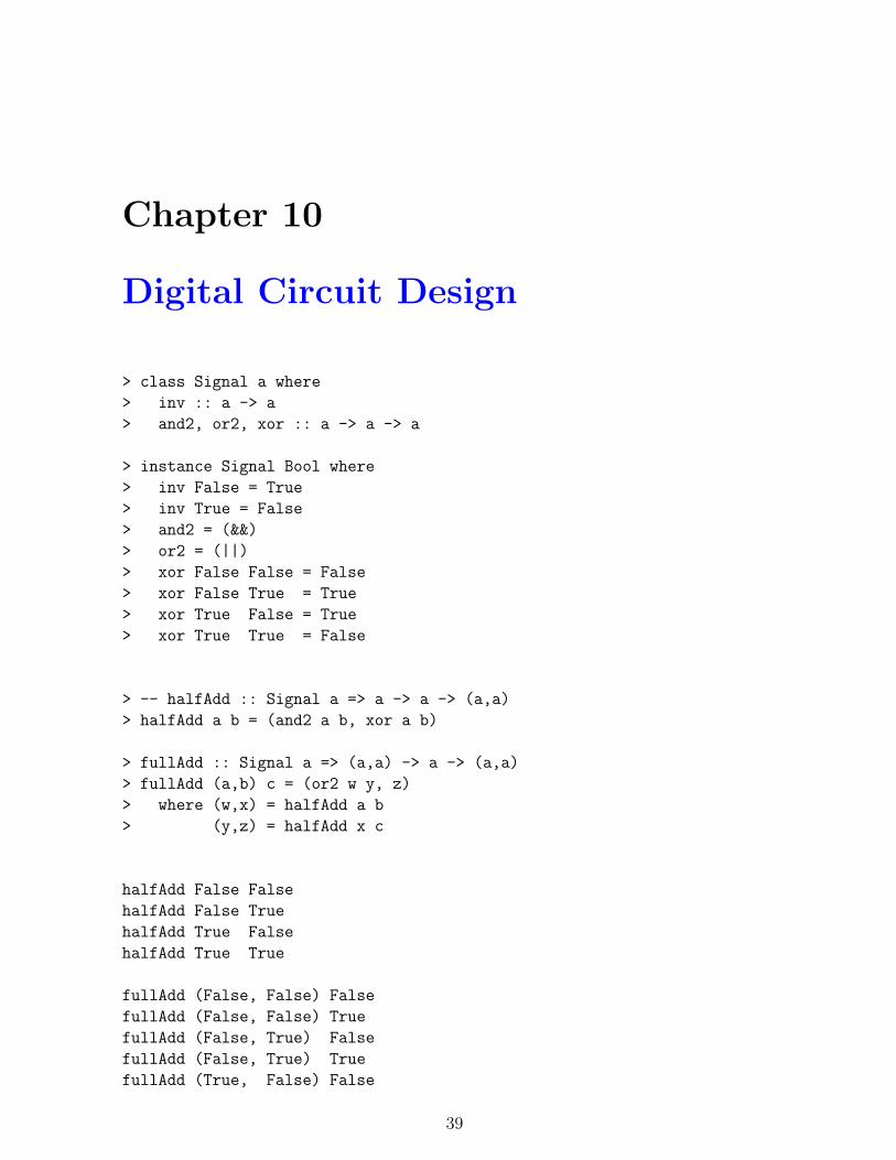
Digital Circuit Design

> class Signal a where

> inv :: a -> a

> and2, or2, xor :: a -> a -> a

> instance Signal Bool where

> inv False = True

> inv True = False

> and2 = (&&)

> or2 = (||)

> xor False False = False

> xor False True = True

> xor True False = True

> xor True True = False

> -- halfAdd :: Signal a => a -> a -> (a,a)

> halfAdd a b = (and2 a b, xor a b)

> fullAdd :: Signal a => (a,a) -> a -> (a,a)

> fullAdd (a,b) c = (or2 w y, z)

> where (w,x) = halfAdd a b

> (y,z) = halfAdd x c

halfAdd False False

halfAdd False True

halfAdd True False

halfAdd True True

fullAdd (False, False) False

fullAdd (False, False) True

fullAdd (False, True) False

fullAdd (False, True) True

fullAdd (True, False) False

39

fullAdd (True, False) True

fullAdd (True, True) False

fullAdd (True, True) True

> add4 :: Signal a => a -> [(a,a)] -> (a,[a])

> add4 c [(x0,y0),(x1,y1),(x2,y2),(x3,y3)] =

> (c0, [s0,s1,s2,s3])

> where (c0,s0) = fullAdd (x0,y0) c1

> (c1,s1) = fullAdd (x1,y1) c2

> (c2,s2) = fullAdd (x2,y2) c3

> (c3,s3) = fullAdd (x3,y3) c

Example: addition of 3 + 8

3 + 8

= 0011 ( 2+1 = 3)

+ 1000 ( 8 = 8)

= 1011 (8+2+1 = 11)

Calculate this by evaluating

add4 False [(False,True),(False,False),(True,False),(True,False)]

The expected result is

(False, [True,False,True,True])

> mscanr :: (b->a->(a,c)) -> a -> [b] -> (a,[c])

> mscanr f a [] = (a,[])

> mscanr f a (x:xs) =

> let (a’,ys) = mscanr f a xs

> (a’’,y) = f x a’

> in (a’’, y:ys)

> rippleAdd :: Signal a => a -> [(a,a)] -> (a, [a])

> rippleAdd c zs = mscanr fullAdd c zs

Example: addition of 23+11

23 + 11

= 010111 (16+4+2+1 = 23)

+ 001011 ( 8+2+1 = 11) with carry input = 0

= 100010 ( 32+2 = 34) with carry output = 0

Calculate with the circuit by evaluating

rippleAdd False [(False,False),(True,False),(False,True),

(True,False),(True,True),(True,True)]

The expected result is

(False, [True,False,False,False,True,False])

40