Software Reliability Model Deterministic Models Probabilistic Models Halstead’s software metric...
21
Software Reliability Model •Deterministic Models •Probabilistic Models Halstead’s software metric McCabe’s cyclomatic complexity metrix Error seeding Failure rate Curve fitting Reliability growth Program structure Input domain NHPP Markov
-
Upload
rudolf-mccarthy -
Category
Documents
-
view
223 -
download
0
Transcript of Software Reliability Model Deterministic Models Probabilistic Models Halstead’s software metric...

Software Reliability Model
•Deterministic Models
•Probabilistic Models
Halstead’s software metric
McCabe’s cyclomatic complexity metrix
Error seeding
Failure rate
Curve fitting
Reliability growth
Program structure
Input domain
NHPP
Markov

Software Reliability Model
Halstead’s Software Metric (1977)
nsinstructio machine ofnumber
program in the errors ofnumber
program theofvolumn
program theoflength
soccurrence operand ofnumber totalthe
soccurrenceoperator ofnumber totalthe
program ain appear that operandsdistinct of numbe the
program ain appear that operatorsdistinct of numbe the
2
1
2
1
I
B
V
N
N
N
n
n
3000
)(log)( 21221
21
VB
nnNNV
NNN

Software Reliability Model
McCabe’s Cyclomatic Complexity Metrix
One should start with 1 for the straight path through the module or subroutine . Then you should add 1 when each time you see one ofthe following keywords: IF, REPEAT, WHILE, FOR, OR, AND.Also you should add 1 for each case in a case statement. In addition,you also should add 1 more if the case statement lacks a default case.If the total score is less than 10, then the code is considered to be of high quality. (McConnel, 1993)

a
b c
ed
Software Reliability Model
McCabe’s Cyclomatic Complexity Metrix
The cyclomatic number V(G) = e - n + 2pwhere e is the number of edged in the control graph in which an edge is equivalent to a branching point in the program (IF, WHILE, REPEAT, and CASE) n is the number of vertices in the control graph and a vertex is equivalent to a sequential block of code in the program, and p is the number of connected elements usually 1
6-5+2*1=3
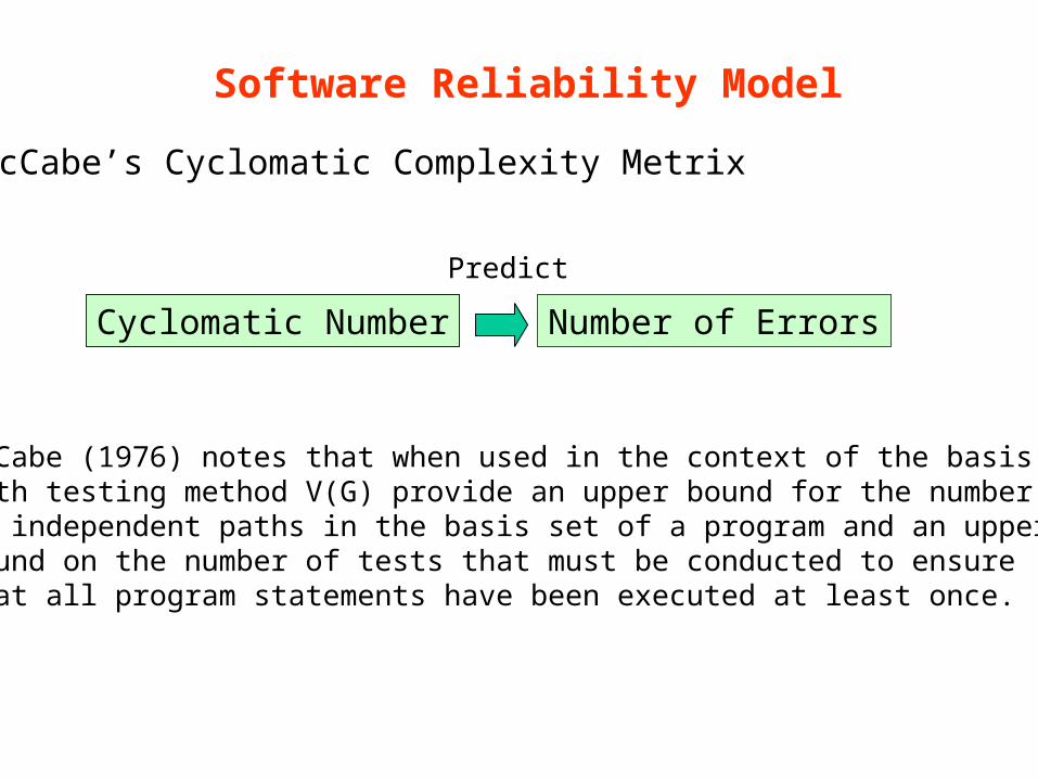
Software Reliability Model
McCabe’s Cyclomatic Complexity Metrix
McCabe (1976) notes that when used in the context of the basispath testing method V(G) provide an upper bound for the number of independent paths in the basis set of a program and an upper bound on the number of tests that must be conducted to ensurethat all program statements have been executed at least once.
Cyclomatic Number Number of Errors
Predict

Software Reliability Model
Error Seeding Models
Operation Profile
Indigenous Error
Pseudo(seeded) Error
Introducing pseudo errors into the program

Software Reliability Model
Error Seeding Models
r
nN
kr
N
k
n
rnnNkp1
1
11 ),,;(
Where N = number of indigenous errors n1= number of induced errors r = number of errors removed during debugging k = number of induced errors in r removed errors r-k = number of indigenous errors in r removed errors
The probability of k induced errors in r removed errors followsa hypergeometric distribution.

Software Reliability Model
Error Seeding Models
Mills, 1970
k
krnN
)(ˆ 1
Maximum likelihood estimate
Type, location, difficulty level
Indigenous errors
Induced errorsSame?

Software Reliability Model
Error Seeding Models
Basin (1980) – two step procedure
One programmer detects n1 errors and a second programmerindependently detects r errors from the same program. Let kbe the common errors found by two programmers.
r
N
kr
nN
k
n
rnNNkp
11
1 ),,;(k
rnN 1ˆ

Software Reliability Model
Failure Rate Models
Assumptions
•The program contains N initial faults•Each error in the program is independent and equally likely to cause a failure during test •Time intervals between occurrences of failure are independent of each other•Whenever a failure occurs, a corresponding fault is removed with certainty•The fault that causes a failure is assumed to be instantaneously removed and no new errors are introduced during the error removal process•The software failure rate during a failure interval is constant and is proportional to the number of faults remaining in the program

Software Reliability Model
Failure Rate Models
Jelinski and Moranda Model (1972)
The program failure rate at the ith failure interval is
)]1([)( iNti
ψ= a proportional constantN = the number of initial errors in the programti = the time between the (i-1)th and ith failure

Software Reliability Model
Failure Rate Models
Jelinski and Moranda Model (1972)
The pdf and cdf of ti are
)))1((())1(()( itiNi eiNtf
itiNi etF ))1((1)(

Software Reliability Model
Failure Rate Models
Jelinski and Moranda Model (1972)
itiNi etR )1()(
Note:
dtttR
tRtdt
tdRtRttf
tfdt
tdR
tR
tft
)()(ln
)()()(
)()()(
)()(
;)(
)()(

Software Reliability Model
Failure Rate Models
Jelinski and Moranda Model (1972)
Suppose that the failure data set {t1,t2,…,tn} is given and ψis known
n
ii
n
i
tiN 11 1
1 N can be solved by
If the parameter ψis also not known
0))1(()(ln
0)1(
1)(ln
1
1 1n
ii
n
i
n
ii
tiNnNL
tiNN
NL

Software Reliability Model
Failure Rate Models
Schick and Wolverton Model (1978)
Assume the failure rate at the ith time interval increases withtime since the last debugging. The program failure rate functionbetween the (I-1)th and the ith failure can be expressed as
ii tiNt )]1([)(
Note: ti is the test time since the (i-1)st failure

Software Reliability Model
Failure Rate Models
Schick and Wolverton Model (1978)
2
)1( 2
)1()(itiN
ii etiNtf
2
)1()(
2
0)(iit
iitiN
dtt
i eetR

Software Reliability Model
Failure Rate Models
Schick and Wolverton Model (1978)
Maximum likelihood estimate
n
ii
n
ii
n
i
tT
T
ti
T
nN
TiN
1
2
1
2
1
where
)1(2
)1(
12

Software Reliability Model
Failure Rate Models
Sukert Modified Schick and Wolverton Model (1977)
Allow more than one failure at each time interval.
iii tnNt ][)( 1
2][
2
1
)(i
it
nN
i etR

Software Reliability Model
Failure Rate Models
Jelinski-Moranda Geometric Model (1979)
Assume the program failure rate function is initially a constantD and decreases geometrically at failure time. The program failurerate and reliability function of time between failures at the ithfailure interval are
)(
)(1
1
ii tDK
i
ii
etR
Dkt
1)(0function geometric ofparameter
where
kk

Software Reliability Model
Failure Rate Models
Lipow Modified Version of the J-M Geometric Model
Allow multiple errors removal in a time interval. The programfailure rate becomes
1)( ini Dkt
where ni-1 is the cumulative number of errors found up to the(i-1)st time interval.

Software Reliability Model
Failure Rate Models
Goel and Okumoto Imperfect Debugging Model
Assume a fault is removed with probability p whenever a failureoccurs.
)]1([)( ipNti
itipNi etR )]1([)(