Software Module Clustering as a Multi–Objective Search Problem

Software Module Clustering as a Multi–Objective Search Problem

Kata Praditwong1, Mark Harman2 and Xin Yao1,3

1The Centre of Excellence for Research in Computational Intelligence and Applications(CERCIA), School of Computer Science, The University of Birmingham,

Edgbaston, Birmingham B15 2TT, UK

2Centre for Research on Evolution, Search and Testing (CREST),Department of Computer Science, King’s College London,

Strand, London WC2R 2LS, UK

3Nature Inspired Computation and Applications Laboratory,Department of Computer Science and Technology,University of Science and Technology of China,

Hefei, Anhui 230027, P. R. China.

May 28, 2009

Abstract

Software module clustering is the problem of automatically organising software units into modules toimprove program structure. There has been a great deal of recent interest in search based formulations ofthis problem, in which module boundaries are identified by automated search, guided by a fitness functionthat captures the twin objectives of high cohesion and low coupling in a single objective fitness function.This paper introduces two novel multi-objective formulations of the software module clustering problem,in which several different objectives (including cohesion and coupling) are represented separately. Inorder to evaluate the effectiveness of the multi-objective approach, a set of experiments were performedon 17 real-world module clustering problems. The results of this empirical study provide strong evidenceto support the claim that the multi-objective approach produces significantly better solutions than theexisting single objective approach.

1 Introduction

Software module clustering is an important and challenging problem in software engineering. It is widelybelieved that a well modularized software system is easier to develop and maintain [8, 27, 29]. Typically, agood module structure is regarded as one that has a high degree of cohesion and a low degree of coupling[8, 27, 29]. Sadly, as software evolves its modular structure tends to degrade [17], necessitating a process ofrestructuring to regain the cognitive coherence of previous incarnations. This paper is concerned with auto-mated techniques for suggesting software clusterings, delimiting boundaries between modules that maximizecohesion while minimizing coupling.

Many authors have considered the implications of software modularization on many software engineer-ing concerns. Badly modularised software is widely regarded as a source of problems for comprehension,increasing the time for on-going maintenance and testing [27, 29, 31]. The use of cohesion and coupling toassess module structure was first popularised by the work of Constantine and Yourdon [8], who introduceda seven-point scale of cohesion and coupling measurement. These levels of cohesion and their measurementhave formed the topic of much work which has sought to define metrics to compute them and to asses theirimpact on software development [1, 3, 25, 14].

There are many ways to approach the module clustering problem. Following Mancoridis et al. who firstsuggested the search based approach to module clustering [20], this paper follows the search based approach.

1

In the search-based approach the attributes of a good modular decomposition are formulated as objectives,the evaluation of which as a ‘fitness function’ guides a search based optimization algorithm.

The module clustering problem is essentially a graph-partitioning problem which is known to be NP-hard [11, 20], so there is no efficient algorithm for solving the problem to its exact optimum unless P=NP [11].This observation provided the motivation for previous work on this problem, which aimed to find a nearoptimal solution within a reasonable amount of time.

Without exception, all previous work on the module clustering problem [20, 19, 23, 10, 22, 18, 15]and other work inspired by it [7] has used a single objective formulation of the problem. That is, thetwin objectives of high cohesion and low coupling have been combined into a single objective called MQ(Modularization Quality) (using weights applied to the measurements of cohesion and coupling). In allstudies reported upon to date, the hill climbing algorithm has performed the best in terms of both thequality of solutions found (measured by MQ values) and in terms of the execution time required to computethem.

However, despite its success, this single objective approach raises the uncomfortable question:

“How much cohesiveness should be sacrificed for an improvement in coupling”

This question, and its converse, are uncomfortable for several reasons. Such questions ignore the factthat the measurements of cohesion and coupling are inherently ordinal scale metrics and so even attemptingto pose such a question contradicts sound measurement theory [28]. Even were it possible to compare thecohesion and coupling measurements on an interval or ratio scale, there is the additional problem that thisessentially requires the mistaken comparison of ‘applies and oranges’; it is not possible to normalise couplingand cohesion in a meaningful way so that each can be measured in comparable units, nor is it easy to decideupon the relative weights that should be applied to each.

There is a natural tension between the objective of achieving low coupling and the objective of achievinghigh cohesion when defining module boundaries. These two aspects of the system will often be in conflict.Therefore, any attempt to conflate cohesion and coupling into a single objective may yield suboptimalresults. In similar software engineering scenarios in which there are a set of two or more possibly conflictingobjectives, a natural step is the use of Pareto optimality [2, 30, 32].

This paper introduces the first Pareto optimal multi-objective formulation of automated software moduleclustering, presenting results that show how this approach can yield superior results to those obtained by thesingle objective formulation. The paper also explores the ways in which the richer solution space affordedby a Pareto optimal approach can be used to yield insight into the choices available to the software engineerfaced with the task of restructuring to improve modular cohesion and coupling.

The primary contributions of the paper are as follows:

1. The multi-objective paradigm for automated software module clustering is introduced. Two formula-tions of the multiple objective approach are studied: the Equal-size Cluster Approach (ECA) and theMaximizing Cluster Approach (MCA).

2. A novel two-archive Pareto optimal genetic algorithm is introduced for the solution of multi-objectivemodule clustering.

3. An empirical study into the effectiveness and performance of the single and multi-objective formulationsof the problem is presented. The primary findings of the study are:

(a) The multi-objective approach is able to produce very strong results for both weighted and un-weighted Module Dependency Graphs. For weighted Module Dependency Graphs, it producesbetter results than the single objective hill climbing approach even when measured against thehill climber’s own fitness function (MQ).

(b) Though the multi-objective approach performs well, there are still cases where the single objectiveapproach can produce good results for unweighted graphs, indicating that hybrid approaches maybe worthy of further consideration for unweighted graphs.

(c) For producing low cohesion and coupling, the Equal-size Cluster Approach to the multi-objectiveproblem produces the best results overall.

(d) The two multi-objective search formulations and the existing single objective formulation searchdifferent parts of the solution space.

2

(e) Though the multi-objective formulations produce far better results, they do so at a computationalcost; two orders of magnitude more effort are required in order to achieve the better results usingthe multi-objective approach. However, the paper argues that, in many practical situations, theadditional time required for better results is both available and also a worthwhile cost for theadditional quality of the modularizations identified.

The rest of this paper or organised as follows. Section 2 presents background material and related workon software module clustering. Section 3 introduces the multi–objective paradigm of module clustering.Section 4 describes the research questions and experiments performed in the empirical study that aims toassess the effectiveness and performance of the multi–objective approach, compared to the single objectiveformulation. Section 5 presents the findings of the empirical study and answers to the research questions.Section 6 discusses the ways in which this work could be used in order to assist the practicing softwareengineer. Section 7 considers threats to validity, while Section 8 concludes.

2 Automated Software Module Clustering

Many metaheuristic methods have been successfully applied to software module clustering. The field wasestablished by the seminal work of the Drexel group [20]. In this work, hill climbing was the primarysearch technique [20], leading to the development of a tool called Bunch [19] for automated software moduleclustering.

Several other metaheuristic search technologies have been applied, including simulated annealing andgenetic algorithms [13, 18, 22]. However, these experiments have all shown that other techniques are out-performed in both result quality and execution time by hill climbing.

In order to formulate software engineering problems as search problems, the representation and fitnessfunction need to be defined [6, 12]. In the case of module clustering, previous work has used the ModuleDependency Graph (MDG) as a representation of the problem [20]. The MDG is represented as a simplearray mapping modules (array indices) to clusters (array elements used to identify clusters) [20]. The array{2, 2, 3, 2, 4, 4, 2, 3} denotes a clustering of 8 modules into 3 clusters, identified by the numbers 2,3 and 4.For example, modules numbered 0,1,3 and 6 are all located in the same cluster (which is numbered 2). Thechoice of numbers of module identifier is arbitrary, so this clustering is equivalent to {1, 1, 3, 1, 4, 4, 1, 3} and{3, 3, 2, 3, 4, 4, 3, 2}.

The MDG can thus be thought of as a graph, in which modules are the nodes and their relationships arethe edges. Edges can be weighted to indicate a strength of relationship or unweighted, merely to indicate thepresence of absence of a relationship. As will be seen, the algorithms studied in this paper differ noticeablyin their performance on weighted MDGs when compared to the results obtained for unweighted MDGsand so this distinction between weighted and unweighted turns out to be an important aspect of problemcharacterisation. The choice of what constitutes a ‘module’ and what precisely can count as a ‘relationship’are parameters to the approach. In previous work (and in the present paper) a module is taken to be a fileand a relationship is an inclusion of reference relationship between files (e.g., a method invocation).

In order to guide the search towards a better modularization it is necessary to capture this notion of a‘better’ modularisation. Traditionally, single objective approaches used the Modularization Quality measure,MQ, introduced by Mancoridis et al. [20]. The intra–edges are those for which the source and target of theedge lie inside the same cluster. The inter–edges are those for which the source and target lie in distinctclusters. MQ is the sum of the ratio of intra-edges and inter-edges in each cluster, called ModularisationFactor (MFk) for cluster k. MFk can be defined as follows:

MFk =

{

0 if i = 0i

i+ 1

2j

if i > 0.(1)

where i is the weight of intra-edges and j is that of inter-edges, that is j is the sum of edge weights for alledges that originate or terminate in cluster k. The reason for the occurrence of the term 1

2j in the above

equation (rather than merely j) is to split the penalty of the inter-edge across the two clusters that connectedby that edge. If the MDG is unweighted then the weights are set to 1.

3

The MQ can be calculated in terms of MF as

MQ =

n∑

k=1

MFk (2)

where n is the number of clusters.The goal of MQ is to limit excessive coupling, but not to eliminate coupling altogether. That is, if we

simply regard coupling as bad, then a ‘perfect’ solution would have a single module cluster containing allmodules. Such a solution would have zero coupling. However, this is not an idea solution because the modulewould not have the best possible cohesion. The MQ measure attempts to find a balance between couplingand cohesion by combining them into a single measurement. The values produced by MQ may be arbitrarilylarge, because the value is a sum over the number of clusters present in a solution and so the MQ functionis not a metric. The aim is to reward increased cohesion with a higher MQ score and to punish increasedcoupling with a lower MQ score.

In order to handle weighted and unweighted graphs using the same approach, an unweighted graph isessentially treated as a weighted graph in which all edges have an identical weight.

3 Software Module Clustering as a Multi-objective Problem

Existing approaches to the twin objectives of high cohesion and low coupling have combined these twoobjectives into a single objective function, with all of the drawbacks to which the introduction of thispaper referred. Pareto optimality is an alternative approach to handling multiple objectives, that retainsthe character of the problem as a multi–objective problem. Using Pareto optimality, it is not possible tomeasure ‘how much’ better one solution is than another, merely to determine whether one solution is betterthan another. In this way, Pareto optimality combines a set of measurements into a single ordinal scalemetric.

The fitness F (x) of a candidate solution vector, x, is defined in terms of the fitness ascribed to x by eachof the constituent fitness functions, fi but this does not yield a single number for an ‘aggregated fitness’.Rather, a relationship is defined on candidate solution vectors, that defines when one solution is superiorto another. Under the Pareto interpretation of combined fitness ‘no overall fitness improvement occurs nomatter how much almost all of the fitness functions improve, should they do so at the slightest expense ofany one of their number’ [12]. More formally, the relation is defined as follows:

F (x1) > F (x2)⇔

∀i.fi(x1) ≥ fi(x2) ∧ ∃i.fi(x1) > fi(x2)

That is, solution x1 is better than another x2 if it is better according to at least one of the individualfitness functions and no worse according to all of the others. Such a solution x1 is said to ‘dominate’ x2. Ifno element of a set X dominates some solution x, then x is said to be non–dominated by X.

A Pareto optimal search yields a set of solutions that are mutually non–dominating and which form anapproximation to the Pareto front. The Pareto front is the set of elements that are not dominated by anypossible element of the solution space. The Pareto front thus denotes the best results achievable; it is theequivalent to the set of globally optimal points in a single objective search. As with the single objectiveformulation, it is not possible to guarantee to locate this globally optimal solution set, merely to attempt toapproximate it as closely as possible.

Each set of objectives leads to a different multi–objective formulation of the problem. In this paper,two sets of objectives will be considered: The Maximizing Cluster Approach and the Equal-size ClusterApproach. These are explained below.

3.1 The Maximizing Cluster Approach

The Maximizing Cluster Approach (MCA) uses the following set of objectives:

• the sum of intra-edges of all clusters (maximizing),

• the sum of inter-edges of all clusters (minimizing),

4

• the number of clusters (maximizing),

• MQ (maximizing),

• the number of isolated clusters (minimizing).

The inter-edges, the intra-edges, and the MQ are used to measure the quality of the system partitioned.An isolated cluster is a cluster that contains only one module. Experience and intuition dictate that isolatedsingle module clusters are uncommon on good modular decompositions and so they are deprecated in theMCA approach by including the number of isolated clusters and an objective to be minimized.

The aim of the MCA measure is to capture the attributes of a good clustering. That is, it will have max-imum possible cohesion (maximizing intra-edges) and minimal possible coupling (minimizing inter-edges).However, it should not put all modules into a single cluster (maximizing the number of clusters) and notproduce a series of isolated clusters (so the number of isolated clusters is minimized).

Since MQ is a well-studied objective function, this is also included as an objective for MCA. This isone of the attractive aspects of a multi–objective approach; one can always include other candidate singleobjectives as one of the multiple objectives to be optimized. The MQ value will tend to increase if there aremore clusters in the system, so it also makes sense to include the number of clusters in the modularizationas an objective. Notice that this objective is in partial conflict with the objective of minimizing the numberof isolated clusters. Furthermore, the relationship between cohesion and coupling is potentially in conflict,making this a non-trivial multi-objective problem.

To illustrate the MCA approach, consider the MDG in Figure 1. The objective values for MCA are asfollows:

• intra-edges of all clusters (cohesion): 6,

• inter-edges of all clusters (coupling): -6,

• the number of clusters: 3,

• MQ: 1.928571,

• the number of isolated clusters: 0.

The sum of inter-edge of all clusters is multiplied by −2 because each edge is counted twice. The numberof isolated clusters is multiplied by −1 (since it is to be minimized).

3.2 The Equal-size Cluster Approach

The Equal-size Cluster Approach (ECA) does not attempt to optimize for the number of clusters in themodularization. However, this does not mean that solutions may not emerge that happen to have a largenumber of clusters. Rather, the number of clusters is left as a implicit consequence of the other optimisationobjectives, allowing the search process the freedom to choose any number of clusters (large or small) thatbest suits the other explicit objectives.

However, the ECA does attempt to produce a modularisation that contains clusters of roughly equal size,thereby decomposing the software system into roughly equal size modules. This tends to mitigate againstsmall isolated clusters and also tends to avoid the presence of one larger ‘god class’ like structure.

The objectives of the ECA are as follows:

• the sum of intra-edges of all clusters (maximizing),

• the sum of inter-edges of all clusters (minimizing),

• the number of clusters (maximizing),

• MQ (maximizing),

• the difference between the maximum and minimum number of modules in a cluster (minimizing).

To illustrate the ECA approach, consider again the example MDG in Figure 1. The set of objectives forECA are assigned as follows:

5

cluster-2

cluster-4

cluster-5

M1

M3

M4

M5

M6

M7

M8

M2

Figure 1: The Module Dependency Graph (MDG) after Clustering by the Two-Archive Algorithm

• intra-edges of all clusters (cohesion): 6,

• inter-edges of all clusters (coupling): -6,

• the number of clusters: 3,

• MQ: 1.928571,

• the difference between the maximum and minimum number of modules in a cluster: 1.

In this paper, these two formulations of the multi–objective clustering problem will be implemented interms of the two-archive multi-objective evolutionary algorithm of Praditwong and Yao [26]. This algorithmhas been applied to other multi–objective problems, but this paper is the first to report on its applicationto the module clustering problem.

4 Experimental Setup

This section describes the experiments conducted to compare the multi-objective and single objective softwaremodule clustering problems.

4.1 Research Questions

1. MQ Value as Assessment Criterion: How well does the two-archive multi–objective search performwhen compared against the Bunch approach using the MQ value as the assessment criterion?

This question compares the two-archive approach to Bunch, using Bunch’s own fitness value. It wouldbe expected that Bunch, optimizing for the single objective of MQ, should be able to outperform thetwo-archive approach, which is optimizing for a balance between this and several other objectives.

2. Cohesion and Coupling: How well does the two-archive algorithm and the Bunch perform at opti-mising each of the two primary software engineering objectives of low coupling and high cohesion?

6

This research question focuses on the primary software engineering objectives of cohesion and cou-pling. Notwithstanding other interesting assessments, these two criteria are those for which automatedsoftware modularization was conceived, so they form a natural topic for investigation in this paper.

3. Pareto Optimality as Assessment Criterion: How good is the Pareto front achieved by the twoapproaches?

This question compares Bunch to the two-archive approach according to the goals of the two-archiveapproach. It would be expected that the two-archive approach would prevail in such a comparison,since it is designed to solve multi-objective problems.

4. Location of Solutions on the Approximated Pareto Front: What do the distributions of thesets of solutions produced by each algorithm look like?

This question is concerned with the qualitative evaluation of the solutions produced. As a qualitativequestion, it is naturally a little more subjective than the other questions. However, it does decomposeinto two related sub–questions, for which a quantitative analysis is possible:

(a) How diverse are the solutions produced?

(b) What is the relationship between the areas of the solution space covered by each approach?

5. Effort: What is the computational expense of executing each of the two approaches in terms of thenumber of fitness evaluations required.

As well as comparing each algorithm for the number of evaluations required, we shall also give eachthe same budget of fitness evaluations (i.e. the same effort) and see whether one out–performs theother for quality of results, as measured by the MQ values obtained and the intra– and extra-edgespresent in the solutions obtained. Finally, we shall also consider the relationship between the size ofthe problem and the effort (measured by the number of fitness evaluations required).

4.2 Test Problems

The experiment studies the application of the algorithms to 17 different MDGs. The numbers of modules varyfrom 20 to over 100. The MDG in this experiment has two types. The first type is unweighted edges and thesecond type is weighted edges as shown in Table 2. In unweighted graphs, an edge denotes a unidirectionalmethod or a variable passed between two modules. The weighted edge is assigned by considering the numberof the number of unidirectional method or variables passed between two modules; the greater the weight,the more dependency between two modules [18].

4.3 Genetic Algorithms

Genetic algorithms use concepts of population and of recombination inspired by Darwinian Evolution [16].A generic genetic algorithm [6] is presented in Figure 2.

An iterative process is executed, initialised by a randomly chosen population. The iterations are calledgenerations and the members of the population are called chromosomes, because of their analogs in naturalevolution. The process terminates when a population satisfies some pre-determined condition (or a certainnumber of generations have been exceeded).

At each iteration (that is each generation), some members of the population are recombined, crossingover elements of their chromosomes. A fraction of the offspring of this union are mutated and, from theoffspring and the original population a selection process is used to determine the new population. Crucially,recombination and selection are guided by the fitness function; fitter chromosomes having a greater chanceto be selected and recombined.

There are many variations on this overall process, but the crucial ingredients are the way in whichthe fitness guides the search, the recombinatory and the population based nature of the process. In theapplication of any genetic algorithm to any problem their is a need for a tuning phase to determine the bestchoice of parameter values governing the likelihood of mutation, crossover and the determintion of the sizeof the population.

7

Set generation number, m:= 0Choose the initial population of candidate solutions, P (0)Evaluate the fitness for each individual of P (0), F (Pi(0))loop

Recombine: P (m) := R(P (m))Mutate : P (m) := M(P (m))Evaluate: F (P (m))Select: P (m + 1) := S(P (m))m := m + 1exit when goal or stopping condition is satisfied

end loop;

Figure 2: A Generic Genetic Algorithm.

4.4 Algorithmic Parameters

The genetic encoding used here, employs the same system as that introduced by Doval et al. for the Bunchsystem [10]. The crossover operator uses single-point crossover and the mutation operator uses single-pointmutation [10].

Algorithmic parameters are dependent on the number of modules (N). The probability of crossover is0.8 if the population size is less than 100. Otherwise, the probability is 1.0. The probability of mutation is0.004log2(N). The population size is 10N and the maximum number of generations is 200N . The total sizeof archives is equal to the size of the population.

The hill-climbing algorithm used in the experiments reported upon here is the Bunch API [19]. Thealgorithm uses the hill-climbing method from the Bunch library with one individual. A first neighbour whichproduces a better result is accepted (this is the ‘first ascent’ hill climbing approach). The output files (indot format) were generated for the detailed level; this output is the lowest level of the Bunch cluster treeand the one that tends to produce the highest value of MQ.

Higher levels than the detailed level are essentially clusters of clusters, which produce a lower value ofMQ. While these meta–clusters may be very useful to engineer, they are not an appropriate choice for anunbiased empirical comparison with the multi–objective approach, because the multi–objective approachalways produces results at the detailed level.

The other parameters are set to their default settings. The information reported, such as the number ofintra-edges, the number of inter-edges, MQ, was calculated from the dot format file.

4.5 Collecting Results from Experiment

Each execution of each algorithm on each MDG was independently repeated 30 times. There are two differentways to calculate the average of the MQ. The hill-climbing algorithm gives only one solution in each run. Theaverage of MQ can calculated indirectly from the solutions. However, the two-archive algorithm producesthe set of solutions. The solution with the highest MQ is chosen to be the best solution in each run.Thus, the average of the MQ of obtained solutions from the two-Archive algorithm is estimated using therepresentatives from 30 runs. This is method to collect the MQ values from experiment.

Both algorithms, the hill-climbing algorithm and the two-archive algorithm, give clustered systems whenthey finish searching. The hill-climbing algorithm has only one system per run, while the two-Archivealgorithm selects the system which corresponds the highest MQ value. The numbers of intra-edges andinter-edges are calculated by analysis the clustered systems, yielded by the algorithms.

5 Results and Analysis

This section presents the results of the empirical study. Each subsection addresses one of the five researchquestions outlined in Section 4. The results concern three algorithms, the Bunch hill-climbing algorithm, andthe two multi-objective formulations of the clustering problem, ECA and MCA, described earlier in Section 3.Table 1 presents details of the subject MDGs studied. These systems are not necessarily ‘degraded’ systems

8

in terms of their modular structure, but they have been studied widely by other researchers to evaluate theiralgorithms for module clustering and so they denote reasonable choices for comparison.

5.1 The MQ Value as Assessment Criterion

This section presents the result of the experiments that compare the MQ values obtained for the threeapproaches. That is, the results assess how well the two multi–objective approaches perform when comparedwith Bunch, using Bunch’s sole criterion: MQ.

Tables 2 and 3 present the results comparing MCA and ECA respectively with the hill climbing approach,while Table 4 shows the comparison of results between the two multi objective approaches (MCA and ECA).Emboldened figures denote comparisons where there is a significant difference (at the 95% confidence level)in the means of MQ values found between the approaches (compared using a two tailed t-test).

In table 2, the results from two algorithms were comparable. There is good evidence to suggest that forthe unweighted problems, the hill-climbing algorithm outperformed the MCA approach. That is, the hill-climbing algorithm gives higher values for MQ in 6 from 7 problems, including 4 problems in which the resultsare statistically significant. However, for weighted MDG problems, the results provide evidence to suggestthat the MCA approach outperforms the hill climbing approach. That is, MCA beats the hill-climbingalgorithms in 7 from 10 problems, including 6 in which the results are statistically significant.

This finding was something of a surprise. One would expect the hill climbing approach to perform wellat optimizing for the single objective MQ, since this is its sole objective. However, there is evidence tosuggest that the multi-objective MCA approach outperforms hill climbing for weighted MDGs (though notunweighted MDGs).

Turning to the results for the ECA multi-objective approach the surprise was even greater. There is noevidence to suggest that the ECA approach is outperformed by the hill climbing approach for unweightedgraphs. However, there is very strong evidence to suggest that the ECA approach outperforms the hillclimber for weighted MDGs. That is, in no unweighted case did either approach outperform the other withstatistical significance. However, for weighted graphs, the ECA approach outperforms the hill climber in allproblems studied with statistically significant differences in the means in all cases.

This set of comparisons of the two multi-objective approaches with the single objective hill climber,provide evidence to suggest that both multi-objective algorithms can outperform the single objective hillclimber when compared using the hill climber’s own sole objective. The results also indicate that, of the twomulti-objective approaches, ECA is to be preferred over MCA. This is borne out by the comparison of theECA and MCA approaches (presented in Figure 4). In all cases the ECA approach outperforms the MCAapproach and, in all but the smallest two, the results are statistically significant.

To answer Research Question 1, the results of the study provide evidence to support the claim that theBunch hill climbing approach produces superior MQ values for unweighted graphs than the MCA approach.However, for weighted graphs, there is strong evidence (from the results in Tables 2 and 3) to suggest thatthe multi-objective research (and in particular the ECA version of the multi-objective search) can producesignificantly better results for MQ values of weighted MDGs compared to the Bunch Hill Climbing approach.There is also very strong evidence to suggest that the ECA approach is superior to the MCA approach interms of MQ values obtained.

One of the primary reasons for such good results is that the multi-objective algorithm always searchesfor a non-dominated set, rather than any single solution. The diversity among the solutions in the set isexplicitly encouraged by the algorithm. As a result, the multi-objective algorithm is more likely to explorewidely in the search landscape. The more complex the search landscape, the more likely the multi-objectivealgorithm performs better. This also explains why our algorithm outperformed the single-objective methodmore on weighted graphs.

It is interesting to speculate as to why the ECA approach should appear to outperform the MCA ap-proach. Clearly more experiments and further study would be required to provide a conclusive answer tothis subsidiary question. However, since the difference rests upon the way in which ECA seeks to normalizecluster size, favouring solutions that minimize the difference between cluster sizes, it must be assumed thatin software systems this is a helpful guide to modularization. By contrast, seeking to punish a solution forcontaining isolated clusters (the MCA approach) is less helpful. In order to explore this further, experi-ments would be required that compared software MDGs to dependence from other (non software) sources.It may turn out that such studies could help to explain what it is that makes a dependence graph a softwaredependence graph rather than a graph in general.

9

5.2 Cohesion and Coupling as Assessment Criteria

This section considers the answer to the second research question, which address the central role playedby cohesion and coupling in all work on module clustering. That is, which approach can produce thehighest cohesion and the lowest coupling? Cohesion is a measure of the number of intra edges in themodularization (those edges that lie inside a cluster), while coupling is measured by the number of interedges in the modularization (the edges that connect two clusters). Both of these objectives are construedas maximization problems in the formulation, so the number of inter edges is represented by the negative ofthe inter edges; the goal is to maximize this value (i.e. to reduce coupling).

Tables 10 to 12 present the results comparing the performance of {MCA, Hill Climbing}, { ECA, HillClimbing} and {MCA, ECA} respectively.

In Table 10, the Comparison of MCA and Hill climbing is somewhat inconclusive for unweighted graphswith each approach able to statistically significantly outperform the other in some cases. However, forweighted MDGs, the MCA approach outperforms the Hill climbing approach in all cases with statisticalsignificance.

In Table 11, the results provide strong evidence to suggest that the ECA approach outperforms the hillclimbing approach for both weighted and unweighted graphs. That is, in all but one of the problems studiedthe ECA approach outperforms the hill climbing approach with statistical significance.

Table 12, provides evidence to suggest that the ECA approach is preferable to the MCA approach; ECAstatistically significantly outperforms MCA in all but one case. However, it is interesting to note that inthe one case where MCA outperforms ECA it also does so with statistical significance. This indicates thatthere remains some residual merit in the MCA approach. This issue of complementarity of approaches isre-visited in Section 5.4.

To answer Research Question 2, there is strong evidence (from Tables 10 and 11) to support the claimthat the multi-objective approach (both the MCA and ECA versions) outperform the Hill Climbing approachin producing solution clusterings with both higher cohesion and lower coupling for weighted graphs. Further-more, there is also strong evidence (from Table 11) that the ECA multi-objective approach can outperformthe Bunch Hill Climbing approach on both weighted and unweighted graphs when aiming to produce solu-tions that minimize coupling, while maximizing cohesion. This provides strong empirical evidence to supportthe claim that the multi-objective approach is worthy of further consideration as an optimally performingapproach to module clustering.

5.3 Pareto Optimality as Assessment Criterion

This section compares the multi-objective formulations with the single objective formulation in terms ofhow well each performs at producing good approximations to the Pareto front. Here, the multi-objectiveformulations can be expected to outperform the single objective formulation, since they are designed toproduce good approximations to the Pareto front, whereas the single objective approach is not. Therefore,the more interesting part of this research question is which of the two multi objective formulations performsbest.

Tables 13 to 15 display the dominance relationship for the results obtained from all three approaches.This dominance relationship is used to compare any two solutions in multi-objective space.

The three software engineering objectives considered are the intra-edge and the inter-edge measurement,and, for backward compatibility with work on single objective formulations, the MQ value obtained. Theseobjectives can be thought of as collectively denoting the quality of the clustering produced.

In these tables, A denotes the hill-climbing algorithm, B denotes the MCA, and C denotes the ECA.The heading NXY denotes the number of solutions generated by X that are dominated by solution in Y . Incomparison, X is better than Y if NXY is small and NY X is large.

Table 13 shows that the number of solutions produced by hill-climbing outperforms MCA for unweightedproblems (6 from 7 problems), while in weighted systems, the MCA outperforms the hill-climbing algorithmin all problems. This indicates that hill climbing is effective, perhaps surprisingly so, for unweighted MDGs.

Table 14, provides strong evidence that ECA outperforms hill climbing for both weighted and unweightedMDGs. That is, the values of NAC are higher than NCA in 16 from 17 of the solutions..

These two findings, taken together, indicate the ECA is better than hill climbing, while MCA is only betterthan hill climbing for weighted graphs, leading to suspicion that ECA outperforms MCA. This suspicion

10

is confirmed by the results from Table 15, which compares ECA and MCA. This table shows that ECAcomfortably outperforms MCA in all of the problems studied.

To answer Research Question 3, as expected the single objective formulation implemented by Bunchis not well suited to finding non-dominated solutions for a set of objectives. The results are particularlycompelling for the ECA multi-objective approach, which comfortably outperforms the other approaches.

5.4 Location of Solutions

This section considers the location of solutions produced by the two approaches. In order to examine thelocation of solutions, it is convenient to compare two of the primary software engineering objectives. For thisreason, cohesion (intra edges) and the MQ value are chosen to see the trade off between these two objectives.The previous sets of experiments have indicated a strong degree of difference between the results of weightedand unweighted MDGs. Therefore, in considering location of solutions, the results are categorized into thosefor weighted MDGs and those for unweighted MDGs. Figure 4 shows the locations of solutions in this twoobjective space for unweighted MDGs, while Figure 5 show the location for unweighted MDGs.

In all figures, the two objectives are to be maximized, so the optimal solutions are located in the uppermostand rightmost areas of the two objective space, while the least optimal are located in the lower-most andleftmost areas of the space. The results in Figure 4 confirm the earlier findings that ECA is to be preferredover MCA for unweighted MDGs and also that hill climbing (labelled HC) is a strong performer on unweightedgraphs. The results in Figure 5 are perhaps a little more interesting. They reveal that each of the threealgorithms concentrates in a different region of the two objective search space. Visually, it is apparent thatthe hill climbing approach tends to concentrate on the less optimal areas of the space, while the both ECAand MCA are focused on more productive locations. However, of ECA and MCA it is not always possible tosay that ECA is the better of the two. This suggests that for optimal results both ECA and MCA should beused. Although the previous studies indicate that ECA will tend to outperform MCA, the visualisation ofresult locations in two dimensional objective space, indicate that the two approaches concentrate on differentareas of the solution space and that MCA is occasionally able to produce results that outperform ECA forone of the two objectives.

To answer Research Question 4, the resulting locations indicate that the three approaches produce solu-tions in different parts of the solution space. This indicates that no one solution should be preferred over theothers for a complete explanation of the module clustering problem. While the results for the ECA multi-objective approach indicate that it performs very well in terms of MQ value, non-dominated solutions andcohesion and coupling, this does not mean that the other two approaches are not worthy of consideration,because the results suggest that they search different areas of the solution space.

It is interesting to note how the different approaches produce solutions in different regions of the solutionspace according to the fitness function values obtained. This suggests that each technique also finds differentre-modularizations of the software, though more work is required to examine this is more detail.

5.5 Computational Effort

This section compares the effort required to solve the clustering problem using the traditional hill climbingapproach and the new multi-objective approaches introduced in this paper. The results indicate that thereis a trade-off between effort and quality of results. That is, the number of evaluations required to achievethe better results of the multi–objective approach is two orders of magnitude greater than that required forthe hill climber. However, even if we allow the Hill Climber the same number of fitness evaluations as themulti-objective approaches, the results for the multi-objective approach are still typically better than thoseobtained by the Hill Climber. Finally, we explore the relationship between the size of the problem and thenumber of fitness evaluations required by the multi-objective approach. This study indicates that there isno obvious relationship between size of problem and effort.

5.5.1 Number of Evaluations

An important factor for search algorithms is a number of evaluations. The number of evaluations indicatesthe computational cost of an algorithm. The numbers of evaluations of all algorithms are shown in Table 5.The two approaches (MCA and ECA) that use the two-archive algorithm use the same number of fixedevaluations. The hill-climbing algorithm will terminate when it can no longer find a neighbour that produces

11

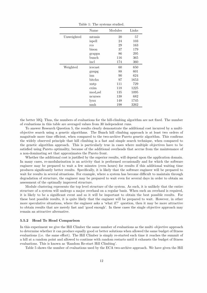
Table 1: The systems studied.

Name Modules Links

Unweighted mtunis 20 57ispell 24 103rcs 29 163bison 37 179grappa 86 295bunch 116 365incl 174 360

Weighted icecast 60 650gnupg 88 601inn 90 624bitchx 97 1653xntp 111 729exim 118 1225mod ssl 135 1095ncurses 138 682lynx 148 1745nmh 198 3262

the better MQ. Thus, the numbers of evaluations for the hill-climbing algorithm are not fixed. The numberof evaluations in this table are averaged values from 30 independent runs.

To answer Research Question 5, the results clearly demonstrate the additional cost incurred by a multi-objective search using a genetic algorithms. The Bunch hill climbing approach is at least two orders ofmagnitude more time efficient, when compared to the two-archive Pareto genetic algorithm. This confirmsthe widely observed principle that hill climbing is a fast and simple search technique, when compared tothe genetic algorithm approach. This is particularly true in cases where multiple objectives have to besatisfied using Pareto optimality, because of the additional overheads that accrue from the maintenance ofa non-dominating set that approximates the Pareto front.

Whether the additional cost is justified by the superior results, will depend upon the application domain.In many cases, re-modularisation is an activity that is performed occasionally and for which the softwareengineer may be prepared to wait a few minutes (even hours) for results if this additional waiting timeproduces significantly better results. Specifically, it is likely that the software engineer will be prepared towait for results in several situations. For example, where a system has become difficult to maintain throughdegradation of structure, the engineer may be prepared to wait even for several days in order to obtain anassessment of the optimally improved structure.

Module clustering represents the top level structure of the system. As such, it is unlikely that the entirestructure of a system will undergo a major overhaul on a regular basis. When such an overhaul is required,it is likely to be a significant event and so it will be important to obtain the best possible results. Forthese best possible results, it is quite likely that the engineer will be prepared to wait. However, in othermore speculative situations, where the engineer asks a ‘what if?’ question, then it may be more attractiveto obtain results that are merely fast and ‘good enough’. In these cases the single objective approach mayremain an attractive alternative.

5.5.2 Head To Head Comparison

In this experiment we give the Hill Climber the same number of evaluations as the multi–objective approachto determine whether it can produce equally good or better solutions when allowed the same budget of fitnessevaluations (i.e. the same effort). The Hill Climber is simply re-started each time it reaches the summit ofa hill at a random point and allowed to continue with random restarts until it exhausts the budget of fitnessevaluations. This is known as ‘Random Re-start Hill Climbing’.

Table 5 shows the number of evaluations used by the ECA two-archive approach. We have given the Hill

12

Table 2: Comparison of solutions found by the MCA approach and Bunch’s Hill Climbing Approach usinga two tailed t-test with 58 degrees of freedom. Figures in bold are significant at the 95% level.

Name MCA Hill-Climbing t-testMean STD Mean STD

Unweighted mtunis 2.294 0.013 2.249 0.060 0.914ispell 2.269 0.043 2.337 0.022 -1.461rcs 2.145 0.034 2.218 0.020 -1.726bison 2.416 0.038 2.639 0.041 -4.331

grappa 11.586 0.106 12.676 0.017 -16.977

bunch 12.145 0.225 13.536 0.054 -14.420

incl 11.811 0.351 13.568 0.035 -15.480

Weighted icecast 2.401 0.057 1.779 0.145 7.574

gnupg 6.259 0.072 4.869 0.168 15.549

inn 7.421 0.077 6.720 0.180 7.571

bitchx 3.572 0.055 2.465 0.200 11.988

xntp 6.482 0.110 6.655 0.151 -1.855exim 5.316 0.132 5.199 0.166 1.174mod ssl 8.832 0.097 7.906 0.293 8.129

ncurses 10.211 0.145 9.836 0.181 3.602

lynx 3.447 0.086 3.488 0.124 -0.494nmh 6.671 0.177 7.012 0.254 -2.847

Table 3: Comparison of solutions found by the ECA approach and Bunch’s Hill Climbing Approach using atwo tailed t-test with 58 degrees of freedom. Figures in bold are significant at the 95% level.

Name ECA Hill-Climbing t-testMean STD Mean STD

Unweighted mtunis 2.314 0.000 2.249 0.060 1.474ispell 2.339 0.022 2.337 0.022 0.042rcs 2.239 0.022 2.218 0.020 0.556bison 2.648 0.029 2.639 0.041 0.177grappa 12.578 0.053 12.676 0.017 -2.017bunch 13.455 0.088 13.536 0.054 -1.171incl 13.511 0.059 13.568 0.035 -1.018


gnupg 6.905 0.055 4.869 0.168 23.663

inn 7.876 0.046 6.72 0.180 13.320

bitchx 4.267 0.027 2.465 0.200 20.703

xntp 8.168 0.076 6.655 0.151 17.400

exim 6.361 0.084 5.199 0.166 12.734

mod ssl 9.749 0.071 7.906 0.293 16.735

ncurses 11.297 0.133 9.836 0.181 14.287

lynx 4.694 0.060 3.488 0.124 15.410

nmh 8.592 0.148 7.012 0.254 13.647

13

Table 4: The Averaged MQ Values of the Best Solutions Found by the Two-Archive Algorithm with Max-imizing Cluster Approach (MCA), and by the Two-Archive Algorithm with Equal-Size Cluster Approach(ECA) and the Value of a two-tailed t-test with 58 degrees of freedom.

Name ECA MCA t-testMean STD Mean STD

Unweighted mtunis 2.314 0.000 2.294 0.013 0.991ispell 2.339 0.022 2.269 0.043 1.496rcs 2.239 0.022 2.145 0.034 2.176

bison 2.648 0.029 2.416 0.038 4.873

grappa 12.578 0.053 11.586 0.106 13.625

bunch 13.455 0.088 12.145 0.225 12.830

incl 13.511 0.059 11.811 0.351 14.535


gnupg 6.905 0.055 6.259 0.072 9.932

inn 7.876 0.046 7.421 0.077 7.101

bitchx 4.267 0.027 3.572 0.055 13.267

xntp 8.168 0.076 6.482 0.110 21.451

exim 6.361 0.084 5.316 0.132 12.321

mod ssl 9.749 0.071 8.832 0.097 12.252

ncurses 11.297 0.133 10.211 0.145 11.288

lynx 4.694 0.060 3.447 0.086 17.870

nmh 8.592 0.148 6.671 0.177 18.476

Climber the same number of evaluations as used in all 30 runs of the ECA algorithm for complete fairness.That is, for example, considering mtunis problem, the number of evaluations of ECA is 800,000 and it isrepeated 30 times (to allow for a meaningful statistical comparison of results earlier in the paper). Thus,the total number of evaluations is 24,000,000. The Hill-Climbing approach was performed until the numberof evaluations passes 24,000,000. The number might slightly exceed this ‘fitness evaluation budget’ becausethe current hill climb is allowed to complete before the budget is checked. This ensures that the Hill Climberis afforded at least the same number of evaluations as the ECA approach. Table 6 shows the number ofevaluations and the number of runs performed by the Hill-Climbing approach.

Table 7 presents the MQ value obtained for each algorithm. Hill-Climbing cannot find better solutionsin terms of MQ when the number of evaluations allowed is increased to the total used by the multi-objectiveapproach. Only for three of the problems, grappa, bunch and incl, does the MQ obtained by Hill-Climbingoutperform that found by the ECA algorithm. In the other problems, the ECA algorithm find better MQvalues than the Hill-Climbing algorithm.

A comparison of intra-edge and inter-edge is shown in the Table 8. Hill-Climbing can find the solutionswith good intra-edge and inter-edge but it does not out-perform ECA for result quality when it has the samenumber of evaluations.

5.6 Exploration of the Relationship between Problem Size and Number of Fit-

ness Evaluations Required

In this section we consider the relationship between the size of the problem and the number of fitnessevaluations required. The results show that there is no apparent relationship between the two. That is,there is no strong correlation between the sizes of systems (listed in Table 1) and the effort expended by thesearch techniques (listed in Tables 5 and 6).

This provides some tentative evidence to suggest that that the difficulty of a problem (for the multi–objective approach) is not a function of problem’s size; the complexity of the problem may not be directlyrelated to its size. However, as one might expect, the larger systems do seem to take more fitness evaluations.More work is required with more systems in order to fully determine whether there is any relationship betweenthe size of the MDG and the number of fitness evaluations required.

14

Table 5: Number of Evaluations by the Two-Archive Algorithm and Hill-ClimbingName Two-Archive Algorithm Hill-Climbing

Mean STDmtunis 800000 934.367 204.558ispell 1152000 1823.333 509.483rcs 1682000 3291 884.664bison 2738000 5388.267 1453.368grappa 14792000 68429.867 27558.047bunch 26912000 138477.767 77102.844incl 60552000 125424.433 45517.068icecast 7200000 17371.733 4379.106gnupg 15488000 55475.033 17871.995inn 16200000 96498.633 43471.544bitchx 18818000 89179.033 34799.29xntp 24642000 126195.533 68732.167exim 27848000 132139.867 68820.241mod ssl 36450000 222008.367 112826.268ncurses 38088000 224815.733 97552.865lynx 43808000 126777.767 48318.278nmh 78408000 805155.400 511547.499

Table 6: Number of Evaluations by the Two-Archive Algorithm and Hill-ClimbingName Hill-Climbing Two-Archive Algorithm

No. of Runs No. of Evaluations No. of Evaluationsmtunis 26014 24000943 24000000ispell 19340 34560557 34560000rcs 15363 50461933 50460000bison 15408 82140104 82140000grappa 5817 443791973 443760000bunch 6346 807430167 807360000incl 12748 1816661431 1816560000icecast 12429 216006356 216000000gnupg 9083 464654717 464640000inn 5434 486010358 486000000bitchx 7264 564579101 564540000xntp 6162 739300758 739260000exim 6647 835468260 835440000mod ssl 4755 1093626809 1093500000ncurses 4965 1143087432 1142640000lynx 9778 1314294774 1314240000nmh 3107 2353426942 2352240000

15

Table 7: The Averaged MQ Values of the Best Solutions Found by the Two-Archive Algorithm with theEqual-Size Cluster Approach (ECA), and by Hill-Climbing (HC).

Name ECA Hill-Climbing T-test:Mean STD Mean STD ECA-HC

Not weighted mtunis 2.314 0 2.242 0.063 6.322

ispell 2.339 0.022 2.334 0.024 0.970rcs 2.239 0.022 2.220 0.022 4.655

bison 2.648 0.029 2.637 0.038 1.447grappa 12.578 0.053 12.677 0.019 -28.480

bunch 13.455 0.088 13.537 0.055 -8.000

incl 13.511 0.059 13.572 0.037 -9.107


gnupg 6.905 0.055 4.946 0.183 58.528

inn 7.876 0.046 6.676 0.188 34.893

bitchx 4.267 0.027 2.444 0.209 47.799

xntp 8.168 0.076 6.636 0.125 66.857

exim 6.361 0.084 5.207 0.172 36.816

mod ssl 9.749 0.071 7.934 0.306 32.523

ncurses 11.297 0.133 9.804 0.182 44.951

lynx 4.694 0.060 3.489 0.131 50.470

nmh 8.592 0.148 7.062 0.265 31.517

Table 8: The Average of the Intra-edges and the Inter-edges of the Best Solutions Found by the Two-ArchiveAlgorithm with the Equal-Size Cluster Approach (ECA), and by Hill-Climbing (HC)

Name ECA Hill-Climbing T-test: T-test:

Intra-edges Inter-edges Intra-edges Inter-edges Intra-edges Inter-edges

Mean STD Mean STD Mean STD Mean STD ECA-HC ECA-HC

Not weighted

mtunis 27 0 -60 0 22.643 3.489 -69.724 6.914 6.839 7.702

spell 30.033 2.798 -145.933 5.595 25.356 3.030 -156.299 5.984 8.449 9.481

rcs 47.567 7.859 -230.867 15.719 36.810 6.742 -253.372 13.446 8.727 9.156

bison 52.800 6.217 -252.400 12.434 40.225 5.944 -278.546 11.855 11.576 12.067

grappa 101.167 8.301 -387.667 16.601 82.167 3.175 -426.675 6.277 32.230 33.457

bunch 111.700 5.305 -504.600 10.611 100.632 5.707 -527.740 11.341 10.601 11.153

incl 140.200 3.836 -439.600 7.673 140.510 9.862 -439.992 19.710 -0.172 0.109

Weighted

icecast 1643.167 208.189 -7569.667 416.378 780.828 227.609 -9295.350 455.216 20.730 20.743

gnupg 1494.167 103.830 -4413.667 207.660 905.158 129.182 -5592.698 258.341 24.946 24.970

inn 1336.900 190.263 -5046.200 380.526 519.048 122.170 -6682.903 244.343 36.428 36.450

bitchx 7840.600 633.068 -35546.800 1266.136 3050.028 939.989 -45128.934 1879.96 27.887 27.890

xntp 1117.967 54.502 -3692.067 109.004 419.447 77.202 -5090.102 154.394 49.495 49.534

exim 3146.567 525.155 -12612.867 1050.310 1029.345 292.284 -16848.317 584.563 39.396 39.406

mod ssl 3476.800 244.174 -11008.400 488.348 1075.909 151.961 -15811.176 303.928 85.855 85.870

ncurses 806.3670 57.515 -2607.267 115.030 367.182 25.005 -3486.637 49.995 94.738 94.875

lynx 3730.633 478.016 -20546.733 956.032 1561.995 263.208 -24885.012 526.420 44.907 44.917

nmh 2704.600 236.782 -18576.800 473.564 1164.043 215.020 -21658.899 430.016 39.016 39.031

16

Problem Nodes Time (Sec.)Mean STD

mtunis 20 8.1 0.711967ispell 24 23.433333 0.773854rcs 29 24 1.144703bison 37 68.533333 10.852406grappa 86 697.7 166.593279bunch 116 1868.533333 409.992324incl 174 6652.4 2006.30093icecast 60 349.266667 29.657741gnupg 88 2900.766667 953.430564inn 90 1111.766667 265.050637bitchx 97 1375.2 116.074411xntp 111 3434.4 1005.104613exim 118 3631.966667 949.306007mod ssl 135 4219.6 740.464793ncurses 138 12298.46667 3617.612308lynx 148 5790.366667 1693.144972nmh 198 14021.46667 2114.663595

Table 9: The Relationship Between Size and ECA Computation Time.

It may be that search problem difficulty is related to problem complexity not problem size and that,should there turn out to be some correlation, then the difficulty of the search might act as some form ofguide as to the complexity of the problem. However, this remains purely speculation at this point.

6 Use of Automated and Semi-Automated Modularization Based

Cohesion and Coupling

Automated approaches to modularization, such as that presented in this paper focus on automated algorithmsthat seek out new partitions of software, maximizing cohesion and minimizing coupling. There have beenempirical studies that show that low coupling and high cohesion are desirable because they tend to becorrelated with a lower propensity to contain faults [4]. However, care is required in extrapolating from thesestudies to the work reported here; it cannot be assumed that automated re-modularization will necessarilyimprove quality attributes such as fault proneness.

Also, it would be wrong to assume that cohesion and coupling are the only requirements for softwaremodule quality. Many other factors have to be taken into account when deciding upon the quality of softwareand no attempt is made in this paper to claim that automatically re-modularized software will necessarilybe less fault prone, nor to suggest that it will have other desirable properties.

Finally, though the approach advocated here is automated, this does not mean that a practicing SoftwareEngineer should simply press a ‘modularize button’ and accept the results of automated modularizationwithout question. Rather, tools that use these automated techniques are more likely to be interactive; thetool merely suggesting candidates for re-modularization, perhaps indicating functions that could be movedto improve measurements of cohesion and coupling. The user of such a tool would then consider thesesuggestions and decide whether or not to accept them.

This paper adds to the previous work on cohesion and coupling by providing automated techniques thatcan be used to make such suggestions. It improves the measurements of cohesion and coupling that can beachieved so that, where there this is desirable, the user will have potentially more interesting suggestionsfrom the tool to consider.

A further interesting practical contribution of this work is the way in which the paper indicates thatmulti objective search techniques can be useful for improving the fitness scores obtained for single objectiveproblems. This is a phenomenon observed in the wider optimization community [5], but to the authorsknowledge, it is the first time that this phenomenon has been demonstrated in Search Based SoftwareEngineering problems.

17

20 40 60 80 100 120 140 160 180 2000

5000

10000

15000

Number of Nodes

Tim

e

Figure 3: The number of nodes and computation time by ECA.

That is, the search for solutions that maximize the widely studied MQ measurement can be improvedby searching for solutions that solve this and several other objectives, as the results in the present paperindicate. This finding seems surprising at first glance; how can adding objectives make a problem easierto solve? The resolution of this apparent paradox is to be found in the way in which the other objectivescontribute guidance to the solution of the primary objective (in this case MQ). This finding may be useful forother SBSE problems; it may be that even essentially single objective SBSE problems can be re-formulatedas multiple objective search problems in which the additional objectives provide guidance to the solution ofthe primary objective and a pareto optimal search can thereby find superior solutions that achieve higherscores for the primary objective.

The application of search based modularization is not merely a technique for application to systems thathave become degraded through ad hoc maintenance, thought it may be particularly useful for such systems.Like all tools to support Software Engineers in their decision making, the approach can be used to raisequestions about modularization choices, even for very well–maintained systems. Where the search basedapproach suggests a re-modularization that will produce a noticeable improvement in cohesion and couplingthis can be a starting point for investigation, even for well behaved systems.

Furthermore, where the automated approach produces a suggestion that is not followed, this may indi-cate a situation where there are hidden dependencies, not reflected in the MDG. These dependencies willbe hidden to the automated tool, but may be known to the engineer. They may cause the engineer toreject the modularization suggestions. In such cases, the tool may have flagged up a need for additionaldesign documentation to record and document such dependencies. The authors’ experience with code leveldependencies from industrial partners indicates that real code does contain many such hidden dependencies.

7 Threats to Validity

For an experiment not involving human subjects, there are two potential threats to validity that need tobe considered. These are threats to external validity and internal validity. External validity (or selectionvalidity) concerns the degree to which the findings can be generalized to the wider classes of subjects fromwhich the experimental work has drawn a sample.

In work on software engineering this is a particular important threat to validity of findings, because ofthe wide range of diverse programs available to any study of their properties. In the experiments reportedupon here, this threat to validity is somewhat mitigated by the fact that the study is concerned witha highly abstract representation of a program: the Module Dependency Graph (MDG). Since there is ahomomorphism that maps many individual programs into a single MDG, the results for a set of MDGs of

18

size C is relevant to a class of programs of cardinally far larger than C.Nonetheless, as with other empirical studies concerning software, care is required in extrapolation from

the results presented in the present paper to the wider class of programs and their weighted and unweightedMDGs. In order to attempt to cater for possible threats to external validity, the empirical study wasconstructed to use a range of MDGs, both weighted and unweighted and ranging in size from small to large.The systems under study were also varied in their application types. However, all systems considered camefrom open source programs and this may affect the degree to which results can be extrapolated. Naturally,it remains possible that non-open source programs will exhibit different behaviour.

Internal validity is the degree to which conclusions can be drawn about the causal effect of independentvariables on the dependent variables. In this experiment, potential threats come from inappropriate statisticaltests or violations of statistical assumptions, inaccurate underlying analysis, and the degree to which thevariables used in the study accurately measure the concepts they purport to measure (a form of constructvalidity).

In this paper the choice of subject MDGs and statistical tests was partly governed by the desire tosupport comparability with other studies. The statistical test used was the t-test. This has been widely usedby researchers comparing results from studies of metaheuristic search algorithms. The MDGs studied havealso been used in other studies [18, 21, 23], facilitating a degree of comparability.

It is important to use a statistical test for significance of results obtained because there is an inherentdegree of random selection in all metaheuristic search algorithms, that the experimental result must takeinto account. It is known that the t test is best suited to normally distributed data. However, there is strongstatistical evidence [9, 24] to suggest that the t–test is robust, even in the presence of significantly skewedand non-normally distributed data, provided the sample sizes are sufficiently large, which they are in thiscase.

It is also important to note that this work neither demonstrates nor implies any necessary associationbetween quality of systems and the modularization produced by the approach used in this paper. Indeed,module quality may depend on many factors, which may include cohesion and coupling, but which is unlikelyto be limited to merely these two factors.

8 Conclusion and Future Work

This paper introduces the multi-objective approach to software module clustering. It introduces two multi-objective formulations of the multi-objective problems and presented results for the application these tech-niques, comparing the results obtained with those from the existing single objective formulation on 17 realworld model clustering problems

The results indicate that one of the two approaches, the Equal Cluster size Approach, is able to producebetter solutions that the existing single objective solution, both in terms of the multiple objectives it aimsto satisfy, but also in terms of the single objective upon which all previous work has focused. This improvedperformance comes at a significantly increased computational cost. For problems in which the softwareengineer is prepared to wait for the optimal re-clustering of their system, the multi–objective approachtherefore has considerable merit.

The multi-objective approach lends itself to extensions to consider other possible objectives with respectto which modularization could take place. Future work could consider such additional objectives. Forexample, we could consider the foot print size of each module, the communications bandwidth (not merelynumber of inter-edges) the location of features found in module. Future work should also consider thedegree to which different approaches produce different kinds of clustering and the underlying reasons for thedifference in the results obtained using the ECA and MCA approach.

9 Acknowledgements

The authors are grateful to Spiros Mancoridis and Brian Mitchell for providing detailed feedback on an earlierversion of this paper and also for many valuable conversations about software module clustering over thepast six years. Spiros and Brian also kindly made available, both the Bunch tool and the MDGs used in thispaper. The authors also are grateful to Kiarash Mahdavi for providing references, discussions and comments.The anonymous referees also provided detailed, thoughtful and constructive advice which helped to improve

19

Table 10: The Average of the Intra-edges and the Inter-edges of the Best Solutions Found by the Two-ArchiveAlgorithm with Maximizing Cluster Approach (MCA), and by Hill-Climbing and the Value of a Two-TailedT-Test with 58 Degrees of Freedom. Figures in bold are significant at the 95% level.

Name MCA Hill-climbing T-test: T-test:Intra-edges Inter-edges Intra-edges Inter-edges Intra-edges Inter-edges

Mean STD Mean STD Mean STD Mean STD

Unweightedmtunis 24.633 2.092 -64.733 4.185 22.600 3.379 -68.800 6.759 4.761 6.733

ispell 23.100 3.220 -159.800 6.440 25.833 3.761 -154.333 7.522 -5.666 -8.013

rcs 45.133 15.335 -235.733 30.669 35.033 5.822 -255.933 11.644 12.027 17.009

bison 40.367 8.231 -277.267 16.463 40.600 6.683 -276.800 13.366 -0.331 -0.468grappa 84.767 11.190 -420.467 22.380 81.900 2.928 -426.200 5.857 4.179 5.910

bunch 73.567 8.324 -580.867 16.648 100.867 4.883 -526.267 9.766 -41.145 -58.188

incl 91.767 14.024 -536.467 28.048 140.967 11.758 -438.067 23.515 -53.073 -75.056

Weightedicecast 1609.900 294.921 -7636.200 589.843 733.467 238.111 -9389.070 476.222 207.923 294.048

gnupg 1104.733 167.834 -5192.530 335.669 887.200 150.659 -5627.600 301.318 66.763 94.417

inn 771.633 162.630 -6176.730 325.260 554.233 158.848 -6611.530 317.696 66.412 93.920

bitchx 7644.633 2703.349 -35938.700 5406.697 3166.267 861.843 -44895.500 1723.685 410.808 580.970

xntp 733.800 109.722 -4460.400 219.445 447.033 99.724 -5033.930 199.448 108.531 153.486

exim 3279.300 563.781 -12347.400 1127.563 1004.267 342.379 -16897.500 684.758 413.948 585.411

mod ssl 2911.733 310.981 -12138.500 621.962 1101.633 144.082 -15758.700 288.165 464.758 657.268

ncurses 574.433 94.392 -3071.130 188.785 368.700 22.927 -3482.600 45.855 104.035 147.128

lynx 2428.567 863.007 -23150.900 1726.014 1567.800 268.807 -24872.400 537.614 140.139 198.186

nmh 2032.267 438.220 -19921.500 876.440 1120.233 213.024 -21745.500 426.048 195.749 276.831

the presentation of the paper. This work is partially supported by EPSRC (Grant Nos. EP/D050863 andEP/0052785) and National Science Foundation of China (Grant No. 60428202).

References

[1] James M. Bieman and Linda M. Ott. Measuring functional cohesion. IEEE Transactions on SoftwareEngineering, 20(8):644–657, August 1994.

[2] Michael Bowman, Lionel Briand, and Yvan Labiche. Multi-objective genetic algorithms to support classresponsibility assignment. In 23rd IEEE International Conference on Software Maintenance (ICSM2007), Los Alamitos, California, USA, October 2007. IEEE Computer Society Press. To Appear.

[3] Lionel C. Briand, Jie Feng, and Yvan Labiche. Using genetic algorithms and coupling measures to deviseoptimal integration test orders. In Software Engineering and Knowledge Engineering (SEKE 02), pages43–50, 2002.

[4] Lionel C. Briand, Sandro Morasca, and Victor R. Basili. Defining and validating measures for object-based high-level design. IEEE Transactions on Software Engineering, 25(5):722–743, September 1999.

[5] Dimo Brockhoff, Tobias Friedrich, Nils Hebbinghaus, Christian Klein, Frank Neumann, and EckartZitzler. Do additional objectives make a problem harder? In Dirk Thierens, editor, Genetic andEvolutionary Computation COnference (GECCO 2007), volume 1, pages 765–772, London, UK, July2007. ACM Press.

[6] John Clark, Jose Javier Dolado, Mark Harman, Robert Mark Hierons, Bryan Jones, Mary Lumkin,Brian Mitchell, Spiros Mancoridis, Kearton Rees, Marc Roper, and Martin Shepperd. Reformulatingsoftware engineering as a search problem. IEE Proceedings — Software, 150(3):161–175, 2003.

[7] Myra Cohen, Shiu Beng Kooi, and Witawas Srisa-an. Clustering the heap in multi-threaded applicationsfor improved garbage collection. In Maarten Keijzer, Mike Cattolico, Dirk Arnold, Vladan Babovic,Christian Blum, Peter Bosman, Martin V. Butz, Carlos Coello Coello, Dipankar Dasgupta, Sevan G.Ficici, James Foster, Arturo Hernandez-Aguirre, Greg Hornby, Hod Lipson, Phil McMinn, Jason Moore,

20

Table 11: The Average of the Intra-edges and the Inter-edges of the Best Solutions Found by the Two-ArchiveAlgorithm with Equal-Size Cluster Approach (ECA), and by Hill-Climbing and the Value of a Two-TailedT-Test with 58 Degrees of Freedom. Figures in bold are significant at the 95% level.

Name ECA Hill-climbing T-test: T-test:Intra-edges Inter-edges Intra-edges Inter-edges Intra-edges Inter-edges



ispell 30.033 2.798 -145.933 5.595 25.833 3.761 -154.333 7.522 8.983 12.704

rcs 47.567 7.859 -230.867 15.719 35.033 5.822 -255.933 11.644 18.559 26.247

bison 52.800 6.217 -252.400 12.434 40.600 6.683 -276.800 13.366 18.605 26.311

grappa 101.167 8.301 -387.667 16.601 81.900 2.928 -426.200 5.857 31.491 44.536

bunch 111.700 5.305 -504.600 10.611 100.867 4.883 -526.267 9.766 18.590 26.290

incl 140.200 3.836 -439.600 7.673 140.967 11.758 -438.067 23.515 -1.063 -1.504


gnupg 1494.167 103.830 -4413.670 207.660 887.200 150.659 -5627.600 301.318 208.397 294.718

inn 1336.900 190.263 -5046.200 380.526 554.233 158.848 -6611.530 317.696 229.433 324.467

bitchx 7840.600 633.068 -35546.800 1266.136 3166.267 861.843 -44895.500 1723.685 662.175 936.457

xntp 1117.967 54.502 -3692.070 109.004 447.033 99.724 -5033.930 199.448 295.911 418.482

exim 3146.567 525.155 -12612.900 1050.310 1004.267 342.379 -16897.500 684.758 398.380 563.395

mod ssl 3476.800 244.174 -11008.400 488.348 1101.633 144.082 -15758.700 288.165 660.230 933.706

ncurses 806.367 57.515 -2607.270 115.030 368.700 22.927 -3482.600 45.855 267.277 377.987

lynx 3730.633 478.016 -20546.700 956.032 1567.800 268.807 -24872.400 537.614 433.486 613.041

nmh 2704.600 236.782 -18576.800 473.564 1120.233 213.024 -21745.500 426.048 409.170 578.654

Table 12: The Average of the Intra-edges and the Inter-edges of the Best Solutions Found by the Two-ArchiveAlgorithm with Equal-Size Cluster Approach (ECA), and by the Two-Archive Algorithm with MaximizingCluster Approach (MCA) and the Value of a Two-Tailed T-Test with 58 Degrees of Freedom. Figures inbold are significant at the 95% level.

Name ECA MCA T-test: T-test:Intra-edges Inter-edges Intra-edges Inter-edges Intra-edges Inter-edges



ispell 30.033 2.798 -145.933 5.595 23.100 3.220 -159.800 6.440 15.481 21.893

rcs 47.567 7.859 -230.867 15.719 45.133 15.335 -235.733 30.669 2.767 3.914

bison 52.800 6.217 -252.400 12.434 40.367 8.231 -277.267 16.463 17.916 25.337

grappa 101.167 8.301 -387.667 16.601 84.767 11.190 -420.467 22.380 20.346 28.774

bunch 111.700 5.305 -504.600 10.611 73.567 8.324 -580.867 16.648 56.575 80.009

incl 140.200 3.836 -439.600 7.673 91.767 14.024 -536.467 28.048 62.772 88.772


gnupg 1494.167 103.830 -4413.670 207.660 1104.733 167.834 -5192.530 335.669 129.413 183.017

inn 1336.900 190.263 -5046.200 380.526 771.633 162.630 -6176.730 325.260 164.813 233.081

bitchx 7840.600 633.068 -35546.800 1266.136 7644.633 2703.349 -35938.700 5406.697 18.582 26.280

xntp 1117.967 54.502 -3692.070 109.004 733.800 109.722 -4460.400 219.445 164.196 232.208

exim 3146.567 525.155 -12612.900 1050.310 3279.300 563.781 -12347.400 1127.563 -22.031 -31.157

mod ssl 3476.800 244.174 -11008.400 488.348 2911.733 310.981 -12138.500 621.962 131.357 185.767

ncurses 806.367 57.515 -2607.270 115.030 574.433 94.392 -3071.130 188.785 103.071 145.764

lynx 3730.633 478.016 -20546.700 956.032 2428.567 863.007 -23150.900 1726.014 194.749 275.417

nmh 2704.600 236.782 -18576.800 473.564 2032.267 438.220 -19921.500 876.440 141.740 200.451

21

Table 13: Results of Dominated Comparison. A: the hill-climbing algorithm and B: the Two-Archive algo-rithm with the maximizing cluster approach.

Name NAB NBA



Table 14: Results of Dominated Comparison. A: the hill-climbing algorithm and C: the Two-Archive algo-rithm with the equal-size cluster approach.

Name NAC NCA



22

16 18 20 22 24 26 282.14

2.16

2.18

2.2

2.22

2.24

2.26

2.28

2.3

2.32

2.34

Intra−edges

MQ

HCMCAECA

18 20 22 24 26 28 30 32 34 362.2

2.22

2.24

2.26

2.28

2.3

2.32

2.34

2.36

2.38

2.4

Intra−edges

MQ

HCMCAECA

mtunis ispell

20 30 40 50 60 70 80 902.05

2.1

2.15

2.2

2.25

2.3

Intra−edges

MQ

HCMCAECA

25 30 35 40 45 50 55 60 652.35

2.4

2.45

2.5

2.55

2.6

2.65

2.7

2.75

Intra−edges

MQ

HCMCAECA

rcs bison

50 60 70 80 90 100 110 120 13011.2

11.4

11.6

11.8

12

12.2

12.4

12.6

12.8

Intra−edges

MQ

HCMCAECA

50 60 70 80 90 100 110 120 13011.5

12

12.5

13

13.5

14

Intra−edges

MQ

HCMCAECA

grappa bunch

60 80 100 120 140 160 18011

11.5

12

12.5

13

13.5

14

Intra−edges

MQ

HCMCAECA

incl

Figure 4: Solutions in the Intra-edge and MQ Space for Unweighted MDGs

23

0 500 1000 1500 2000 25001.4

1.6

1.8

2

2.2

2.4

2.6

2.8

Intra−edges

MQ

HCMCAECA

600 800 1000 1200 1400 1600 18004

4.5

5

5.5

6

6.5

7

Intra−edges

MQ

HCMCAECA

icecast gnupg

200 400 600 800 1000 1200 1400 1600 18006.4

6.6

6.8

7

7.2

7.4

7.6

7.8

8

Intra−edges

MQ

HCMCAECA

0 5000 10000 150002

2.5

3

3.5

4

4.5

Intra−edgesM

Q

HCMCAECA

inn bitchx

300 400 500 600 700 800 900 1000 1100 1200 13006

6.5

7

7.5

8

8.5

Intra−edges

MQ

HCMCAECA

500 1000 1500 2000 2500 3000 3500 4000 4500 5000

5

5.2

5.4

5.6

5.8

6

6.2

6.4

6.6

Intra−edges

MQ

HCMCAECA

xntp exim

500 1000 1500 2000 2500 3000 3500 4000 45007

7.5

8

8.5

9

9.5

10

Intra−edges

MQ

HCMCAECA

300 400 500 600 700 800 900 10009.5

10

10.5

11

11.5

12

Intra−edges

MQ

HCMCAECA

mod ssl ncurses

1000 1500 2000 2500 3000 3500 4000 4500 50003.2

3.4

3.6

3.8

4

4.2

4.4

4.6

4.8

5

Intra−edges

MQ

HCMCAECA

500 1000 1500 2000 2500 3000 35006

6.5

7

7.5

8

8.5

9

Intra−edges

MQ

HCMCAECA

lynx nmh

Figure 5: Solutions in the Intra-edge and MQ Space for Weighted MDGs

24

Table 15: Results of Dominated Comparison. B: the Two-Archive algorithm with the maximizing clusterapproach and C: the Two-Archive algorithm with the equal-size cluster approach.

Name NBC NCB



Guenther Raidl, Franz Rothlauf, Conor Ryan, and Dirk Thierens, editors, GECCO 2006: Proceedingsof the 8th annual conference on Genetic and evolutionary computation, volume 2, pages 1901–1908,Seattle, Washington, USA, 8-12 July 2006. ACM Press.

[8] Larry L. Constantine and Edward Yourdon. Structured Design. Prentice Hall, 1979.

[9] L. Devroye. Non-Uniform Random Variate Generation. Springer-Verlag, New York, NY 10010, 1986.

[10] D. Doval, S. Mancoridis, and B. S. Mitchell. Automatic clustering of software systems using a ge-netic algorithm. In International Conference on Software Tools and Engineering Practice (STEP’99),Pittsburgh, PA, 30 August - 2 September 1999.

[11] M.R. Garey and D.S. Johnson. Computers and intractability. A Guide to the theory of NP-completeness.WH Freeman and Company, New York, 1979.

[12] Mark Harman. The current state and future of search based software engineering. In Lionel Briand andAlexander Wolf, editors, Future of Software Engineering 2007, Los Alamitos, California, USA, 2007.IEEE Computer Society Press. This volume.

[13] Mark Harman, Robert Hierons, and Mark Proctor. A new representation and crossover operator forsearch-based optimization of software modularization. In GECCO 2002: Proceedings of the Geneticand Evolutionary Computation Conference, pages 1351–1358, San Francisco, CA 94104, USA, 9-13 July2002. Morgan Kaufmann Publishers.

[14] Mark Harman, Margaret Okunlawon, Bala Sivagurunathan, and Sebastian Danicic. Slice-based mea-surement of coupling. In Rachel Harrison, editor, 19th ICSE, Workshop on Process Modelling andEmpirical Studies of Software Evolution, Boston, Massachusetts, USA, May 1997.

[15] Mark Harman, Stephen Swift, and Kiarash Mahdavi. An empirical study of the robustness of twomodule clustering fitness functions. In Genetic and Evolutionary Computation Conference (GECCO2005), pages 1029–1036, Washington DC, USA, June 2005. Association for Computer Machinery.

[16] John H. Holland. Adaption in Natural and Artificial Systems. MIT Press, Ann Arbor, 1975.

25

[17] M. M. Lehman. On understanding laws, evolution and conservation in the large program life cycle.Journal of Systems and Software, 1(3):213–221, 1980.

[18] Kiarash Mahdavi, Mark Harman, and Robert Mark Hierons. A multiple hill climbing approach tosoftware module clustering. In IEEE International Conference on Software Maintenance, pages 315–324, Los Alamitos, California, USA, September 2003. IEEE Computer Society Press.

[19] Spiros Mancoridis, Brian S. Mitchell, Yih-Farn Chen, and Emden R. Gansner. Bunch: A clustering toolfor the recovery and maintenance of software system structures. In Proceedings; IEEE InternationalConference on Software Maintenance, pages 50–59. IEEE Computer Society Press, 1999.

[20] Spiros Mancoridis, Brian S. Mitchell, C. Rorres, Yih-Farn Chen, and Emden R. Gansner. Using auto-matic clustering to produce high-level system organizations of source code. In International Workshopon Program Comprehension (IWPC’98), pages 45–53, Los Alamitos, California, USA, 1998. IEEE Com-puter Society Press.

[21] Brain S. Mitchell. A Heuristic Search Approach to Solving the Software Clustering Problem. PhD Thesis,Drexel University, Philadelphia, PA, January 2002.

[22] Brian S. Mitchell and Spiros Mancoridis. Using heuristic search techniques to extract design abstrac-tions from source code. In GECCO 2002: Proceedings of the Genetic and Evolutionary ComputationConference, pages 1375–1382, San Francisco, CA 94104, USA, 9-13 July 2002. Morgan Kaufmann Pub-lishers.

[23] Brian S. Mitchell and Sprios Mancoridis. On the automatic modularization of software systems usingthe bunch tool. IEEE Transactions on Software Engineering, 32(3):193–208, 2006.

[24] L. E. Moses. Think and Explain with Statistics. Addison-Wesley Publ. Co., Reading, MA, 1986.

[25] Keith Phalp and Steve Counsell. Coupling trends in industrial prototyping roles: An empirical investi-gation. Software Quality Journal, 9(4):223–240, 2001.

[26] K. Praditwong and X. Yao. A New Multi-objective Evolutionary Optimisation Algorithm: The Two-Archive Algorithm. In Y.-M. Cheung, Y. Wang, and H. Liu, editors, Proceedings of the 2006 Interna-tional Conference on Computational Intelligence and Security, volume 1, pages 286–291, Guangzhou,China, 2006.

[27] Roger Pressman. Software Engineering: A Practitioner’s Approach. McGraw-Hill Book CompanyEurope, Maidenhead, Berkshire, England, UK., 3rd edition, 1992. European adaptation (1994). Adaptedby Darrel Ince. ISBN 0-07-707936-1.

[28] Martin J. Shepperd. Foundations of software measurement. Prentice Hall, 1995.

[29] Ian Sommerville. Software Engineering. Addison-Wesley, 6th edition, 2001.

[30] Shin Yoo and Mark Harman. Pareto efficient multi-objective test case selection. In InternationalSymposium on Software Testing and Analysis (ISSTA’07), pages 140 – 150, London, United Kingdom,July 2007. Association for Computer Machinery.

[31] Liguo Yu, Stephen R. Schach, Kai Chen, and A. Jefferson Offutt. Categorization of common couplingand its application to the maintainability of the linux kernel. IEEE Transactions on Software Eng,30(10):694–706, 2004.

[32] Yunayuan Zhang, Mark Harman, and Afshin Mansouri. The multi-objective next release problem.In GECCO 2007: Proceedings of the 9th annual conference on Genetic and evolutionary computation,pages 1129 – 1137, London, UK, July 2007. ACM Press.

26

Software Module Clustering as a Multi–Objective Search Problem

Documents

Transcript of Software Module Clustering as a Multi–Objective Search Problem