SOCIAL INTERACTION AND URBAN SPRAWL

JAN K. BRUECKNER ANN G. LARGEY

CESIFO WORKING PAPER NO. 1843 CATEGORY 8: RESOURCES AND ENVIRONMENT

NOVEMBER 2006

An electronic version of the paper may be downloaded • from the SSRN website: www.SSRN.com • from the RePEc website: www.RePEc.org

• from the CESifo website: Twww.CESifo-group.deT

CESifo Working Paper No. 1843

SOCIAL INTERACTION AND URBAN SPRAWL

Abstract Various authors, most notably Putnam (2000), have argued that low-density living reduces social capital and thus social interaction, and this argument has been used to buttress criticisms of urban sprawl. If low densities in fact reduce social interaction, then an externality arises, validating Putnam’s critique. In choosing their own lot sizes, consumers would fail to consider the loss of interaction benefits for their neighbors when lot size is increased. Lot sizes would then be inefficiently large, and cities excessively spread out. The paper tests the premise of this argument (the existence of a positive link between interaction and density) using data from the Social Capital Benchmark Survey. In the empirical work, social interaction measures for individual survey respondents are regressed on census-tract density and a host of household characteristics, using an instrumental-variable approach to control for the potential endogeneity of density.

JEL Code: R1, J11.

Jan K. Brueckner Department of Economics

University of California, Irvine 3151 Social Science Plaza

Irvine, CA 92697 USA

jkbrueck@uci.edu

Ann G. Largey Dublin City University Business School

Dublin 9 Ireland

alargey@uci.edu

October 2006

Social Interaction and Urban Sprawl

by

Jan K. Brueckner and Ann G. Largey

1. Introduction

Urban sprawl has become a hot policy issue in the United States over the last decade.

Critics of sprawl argue that urban expansion leads to an undesirable sacrifice of farmland along

with a loss of amenity benefits from open space on the urban fringe. The longer commutes

caused by sprawl are thought to create excessive traffic congestion and air pollution, and

sprawl’s suburban focus is viewed as depressing the incentive to revitalize decaying downtown

areas. Finally, commentators such as Putnam (2000) argue that the low-density suburban

lifestyle associated with sprawl reduces social capital, leading to a less-healthy society.1

In response to these concerns, local governments have adopted a wide range of antisprawl

measures, including urban growth boundaries (UGBs) and other related zoning policies, public

land-purchase programs designed to protect vacant land, and price-based mechanisms such as

impact fees that are designed to slow the pace of development. See Brueckner (2001) for an

overview of such policies; Nechyba and Walsh (2005) and Glaeser and Kahn (2006) offer further

discussion.

In appraising the attack on sprawl, Brueckner (2000, 2001) argues that criticism of urban

spatial expansion is only justified in the presence of market failures or other distortions, which

bias the normal expansionary effects of population and income growth in an upward direction.

Such distortions might include a failure by developers to account for the amenity value of

fringe open space in their development decisions, and the failure of commuters to account for

the congestion externalities they generate. The first failure leads to excessive conversion of

agricultural land, while the second leads to overly long commute trips, and both effects imply

excessive spatial expansion of cities. The remedy for the first failure would be higher tax on

urban development, designed to charge the developer for lost open-space amenities, and the

remedy for the second would be congestion pricing of roadways.2

1

The purpose of the present paper is to consider a different market failure, one associated

with social interaction, and to assess whether this failure is empirically relevant as a basis

for criticism of urban sprawl. The starting point of the analysis is the above allegation that

sprawling, low-density development weakens social capital and thus the level of social interac-

tion. While such an effect, by itself, is not the basis of a proper anti-sprawl argument, the case

is different if the nexus between social interaction and density involves an externality.

To understand the argument, suppose that people value social interaction,3 and that the

extent of interaction in a neighborhood is an increasing function of the area’s average popula-

tion density. By putting people in close proximity, high average density could plausibly spur

interaction among them. Average density in a particular household’s neighborhood depends,

in turn, on its own consumption of living space as well as the space consumption levels of its

neighbors.

In choosing space consumption, a household would consider the direct gains from having

more room, along with the negative effect on the social interaction it enjoys, caused by the drop

in neighborhood population density due to its larger residence. But the household would fail to

consider the external effects of consuming more space, which consist of less social interaction

for all its neighbors, again a consequence of lower neighborhood density. The result is a density

externality, which makes space consumption inefficiently high for each household, an effect that

translates into an inefficiently low level of population density for the neighborhood. Because

this argument can be replicated city-wide, it implies inefficiently low density throughout the

urban area, and thus inefficient spatial expansion of the entire city. Thus, the existence of a

density externality based on social interaction can provide another basis for criticism of urban

sprawl.4

A simple model developing this idea is presented in section 2. But the main goal of

the paper is to appraise the empirical relevance of an anti-sprawl argument based on social

interaction. This task requires an empirical test of the underlying hypothesis, which asserts that

social interaction is an increasing function of population density. If this hypothesis is validated,

then the existence of a density externality follows naturally, leading to the conclusion that the

spatial expansion of cities is excessive.

2

The paper uses data from the Social Capital Benchmark Survey, which provides a number of

different measures of social interaction for individual survey respondents in a national sample,

while identifying the census tract where each respondent lives. With the tract identity known,

population density can be computed for each survey respondent’s “neighborhood.” This density

measure is then used as a right-hand variable in a regression explaining social interaction,

which also includes a variety of demographic indicators as covariates. The social interaction

measures that are used include a count of the respondent’s number of close friends, an indicator

of whether the respondent has someone to “confide in,” and related variables.

Similar exercises have been carried out by Glaeser and Gottlieb (2006) and Borck (2006),

focusing more broadly on the determinants of social capital, which includes political involve-

ment and civic engagement in addition to measures of social interaction. Glaeser and Gottlieb

relate their social capital indicators to suburban vs. city residence, and Borck investigates how

social capital is affected by city size.

In addition to its narrower focus, the present paper differs from both these studies by

measuring the key determinant of interaction (here, density) at a disaggregated, census-tract

level. This approach raises an econometric issue that was not a major factor in the previous

studies. In particular, with the census tract of residence being a choice variable of the sur-

vey respondent, it cannot be treated as an exogenous determinant of social interaction. For

example, if social interaction indeed rises with density, then an unusually interactive person

(one with unobservable characteristics highly favorable to interaction) might select a dense

census tract in seeking a congenial place of residence. With this behavior, density would be

positively correlated with the error term in a social-interaction regression, leading to a biased

and inconsistent estimate of its coefficient. Such correlation could also be generated by other

kinds of location behavior.

The empirical work uses an instrumental-variables approach to handle this endogeneity

problem. Since none of the demographic variables available in the survey can be plausibly ex-

cluded as a determinant of interaction, different instruments were sought. The chosen variables

are measures of population density at a more-aggregated level: the first is population density

for the urbanized area containing the census tract, and the second is density for the tract’s

3

MSA. These average density measures are strong determinants of population densities in in-

dividual census tracts. Their use, however, presumes that the endogeneity problem involving

tract density does not extend to the metro level. In other words, while people may self-select

across tracts in endogenous fashion, their choice of a metro area (and hence metro density) is

presumed to be unrelated to unobservable characteristics affecting social interaction.5

Following the theoretical discussion in the next section, the data and variables are described

in section 3, and empirical findings are presented in section 4. Section 5 offers conclusions.

2. Modeling the Density Externality

A density externality can be modeled in the context of a monocentric city, as seen in Fujita

(1989, Ch. 7). However, a simpler spatial structure comes from assuming that individual land

parcels are arbitrarily clustered together in space without the attractive force of a central

business district. For further simplification, suppose that people consume land directly, with

housing capital suppressed, and let consumer i’s land consumption (lot size) be denoted qi.

The spatial area of the city, denoted A, is then found by adding the individual lot sizes, so

that A =∑n

j=1 qj, where n is the number of consumers.

In addition to lot size, consumer i cares about non-land consumption expenditure, denoted

ci, and social interaction, denoted Ii. Preferences, assumed for simplicity to be the same for

all consumers, are given by the well-behaved utility function U(qi, ci, Ii). For simplicity, the

level of social interaction is also assumed to be uniform, and it depends on the city’s average

population density, which equals n/A. While under a more realistic approach, Ii might depend

only on the average densities of the lots near i’s, this change would only introduce inessential

complications in the model. As seen below, however, this local approach to measurement of

density is followed in the empirical work.

Given the above assumptions, the level of interaction can be written Ii = f(n/A), with

f being a smoothly increasing function under a positive density effect (so that f ′ > 0).6

For completeness, however, it is helpful to also consider the possibility that a higher density

reduces interaction, as assumed by Fujita (1989).7 In this case, f(·) is a decreasing function,

with f ′ < 0.

4

Land is assumed to be available at a fixed opportunity cost r, so that consumer i’s budget

constraint is ci + rqi = y, where y is the common level of income. Eliminating ci, the objective

function for consumer i is then given by

U[y − rqi, qi, f

(n/

∑qj

)]. (1)

The consumer chooses qi to maximize (1), taking the lot sizes of other consumers, qk, k �= i,

as parametric. The first-order condition is

−rUc + Uq − UI nf ′

(∑

qj)2= 0, (2)

where superscripts denote partial derivatives. Since consumers are identical, the resulting Nash

equilibrium is symmetric, with∑

qj = nq, where q is the common lot size. Rearranging and

imposing symmetry, (2) becomes

Uq

Uc= r +

f ′

nq2

UI

Uc. (3)

If the density effect is positive, this condition says that lot size is optimal when the consumption

benefit from a marginal increase in q, given by the MRS term on the left, is equal to the money

cost per unit of land, r, plus a cost from reduced interaction, as captured by the last term.

This cost is equal to the marginal benefit of interaction (the MRS term) times the reduction

in the interaction enjoyed by the consumer when his lot size increases (the f ′/nq2 term).

Because consumers ignore the density externality, the equilibrium characterized by (3)

is inefficient. The social optimum can be found by imposing symmetry at the outset and

maximizing the utility of a representative consumer. The objective function is then U [y −rq, q, f(1/q)], where density is given by n/nq = 1/q. The first-order condition for this

problem is

Uq

Uc= r +

f ′

q2

UI

Uc, (4)

5

where f ′/q2 gives the loss of interaction when lot size is increased simultaneously for all con-

sumers. Since the 1/n factor in the last term of (3) is smaller than unity, it follows that the

interaction-cost term in (4) is larger than the corresponding term in (3). As a result, the MRS

on the left-hand side is larger at the social optimum than at the Nash equilibrium, which will

tend to make the socially optimal lot size, denoted q∗, smaller than the equilibrium size, de-

noted qe. This conclusion is assured, for example, if preferences are additively separable in I ,

so that the MRS term on the left of (3) and (4) is independent of the level of social interaction.

Since qe > q∗, it follows the equilibrium spatial size of the city, denoted Ae ≡ nqe, is larger

than the optimal size, A∗ ≡ nq∗. Thus, the equilibrium is characterized by inefficient spatial

expansion of the urban area, providing a basis for criticism of urban sprawl.

The social optimum can be supported by a tax per unit of land consumption, denoted t,

which would appear as an extra term on the RHS of the equilibrium condition (3). This tax

must make (3)’s RHS equal to the RHS of (4), evaluated at the optimum. Equating the two

expressions, the tax is given by

t =(n − 1)f∗′

nq∗2U i∗

Uc∗ , (5)

where the asterisks on f and the marginal utilities indicate that these expressions are evaluated

at the social optimum. Recalling from above that the expression in (5), absent the n−1 factor,

gives one consumer’s loss from lower interaction when his lot size increases, it follows that the

tax serves to charge the consumer for the equivalent losses suffered by his n − 1 neighbors.

With the externality thus internalized, the equilibrium under taxation is efficient.

By contrast, if the density effect is negative, with f ′ < 0, then the second term in (4) is

negative, and qe < q∗. Individual lot sizes are thus too small, and the city is insufficiently spread

out rather than too large. In this case, t in (5) is negative, indicating that land consumption

should be subsidized, not taxed, to support the social optimum.

When the density effect is positive, an urban growth boundary can be used to generate

the optimum. An upper bound of A∗ would be imposed on the spatial size of the city via

zoning regulations, and this restriction in land supply would cause the land price to rise above

6

its opportunity cost. The new equilibrium would be characterized by (3), with r replaced by

an endogenous land rent r, along with the condition∑

qj = A∗. It is easy to see that the

equalities q = q∗ and r = r + t hold in equilibrium.

By contrast, a different type of quantity restriction is needed to address the inefficiency

caused by a negative density effect. In this case, a minimum-lot-size regulation, which requires

q ≥ q∗, must be imposed.

The preceding analysis shows that, if social interaction is an increasing function of pop-

ulation density, then the uncoordinated choices of consumers will lead to lot sizes that are

inefficiently large and a city that takes up too much space. The remainder of the paper is de-

voted to testing the premise of this argument, namely, that interaction increases with density.

3. Data and Variables

The data are drawn from the Social Capital Benchmark Survey, which was carried out

by the Saguaro Seminar at Harvard’s Kennedy School of Government and is disseminated by

the Roper Center for Public Opinion Research at the University of Connecticut (www.roper.

uconn.edu). The survey posed hundreds of social-capital questions to a nationwide sample of

over 30,000 respondents. A restricted version of the data identifies each respondent’s census

tract, allowing accurate measurement of local population density. Given the focus on urban

sprawl, attention is restricted to those respondents living in the urbanized-area portions of

MSAs (thus excluding rural areas), which reduces the sample size to 14,827 individuals. Be-

cause most of the social interaction variables, which are described next, have a small number

of missing values, the effective sample sizes are usually slightly smaller than this number.

The analysis focuses on variables narrowly measuring social interaction, not including

broader indicators of social capital. The variables, whose full definitions are given in Table 1

along with summary statistics, fall into two sets. The first set consists of variables measuring

the extent of the respondent’s neighborhood contacts and friendships. NEISOC measures

how often the respondent socializes with neighbors; NEITALK is a dummy variable indicating

whether this interaction occurs at least once a week; CONFIDE counts the number of people

the respondent can confide in; FRIENDS counts the number of close friends; FRNDHNG

7

measures the frequency of “hanging out” with friends in a public place; FRNDHOM measures

the frequency with which friends are invited to the respondent’s home.

The second set of variables measures the respondent’s group involvement. NEICOOP is a

dummy indicating cooperation with neighbors to get something fixed or improved; GRPHOB is

a dummy indicating membership in a hobby-oriented club; CCLUBMET counts the frequency

of attendance at any club meetings over the previous twelve months; GRPINVLV counts the

number of formal non-church groups to which the member belongs.

The various social-interaction measures are used as dependent variables in separate regres-

sions. In addition to tract-level population density, which is measured in log form and denoted

LNPDEN TRACT, many demographic covariates are used in these regressions. While full

details and variable names are listed in Table 1, these variables include the measures of the

respondent’s sex, age, race, income, education, region of residence, and marital, employment

and citizenship status. Other variables capture the presence of children in the household and

whether the respondent has lived in the area for more than 5 years. While the effects of many

of these variables on social interaction are hard to predict a priori, marriage (or living with

a partner) might lead to more interaction given that couples can benefit from one another’s

acquaintances. In addition, since many adult social bonds are made through child-related ac-

tivities, the presence of children should raise the level of interaction. Since long-time residents

have had more opportunity to build social linkages, they should exhibit higher interaction

than recent arrivals. Lacking social connections at work, unemployed respondents would be

expected to interact less than their employed counterparts. Since non-citizens may not be well

integrated into U.S. society, they may engage in less social interaction than citizens.

It could be argued that marital status (and thus ultimately the presence of children)

depends on the interactive tendencies of an individual, with weak interactors less likely to

become married. This view suggests that MAR PART and the two KIDS variables could

be viewed as endogenous, making them inappropriate as right-hand variables in an equation

explaining interaction. To address this possibility, specifications without these variables are

also estimated, with the results reported following presentation of the main estimates. The

HOMEMAKER variable is also dropped in these equations.

8

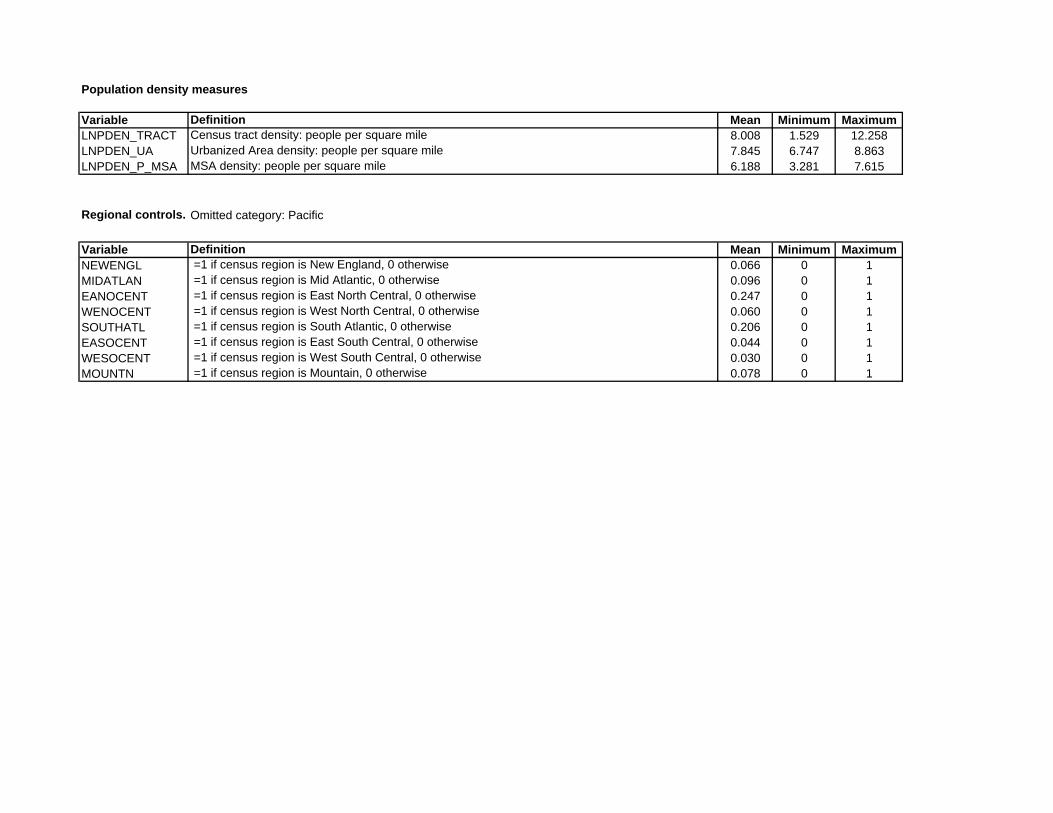
As indicated above, the instruments for tract population density are the log of average

density for the urbanized area containing the tract (LNPDEN UA), and the log of average

density for the tract’s MSA (LNPDEN MSA). While urbanized-area density may be most

relevant as a determinant of the densities of individual census tracts, all of which are in urban-

ized areas, MSA density provides additional information. In particular, holding LNPDEN UA

fixed, MSA density helps to capture population densities in the rural portions of an MSA, out-

side its urbanized areas. This role can be seen in Table 1, which reveals that MSA density

has a lower sample mean than urbanized-area density, reflecting the rural component. Rural

density, in turn, is a good predictor of the minimum density in the urbanized area, which is

achieved at the urban fringe. Thus, information on rural density (via LNPDEN MSA) and

average density for the urbanized-area pins down two points on the area’s spatial distribution

of population densities. As a result, use of both variables as instruments seems warranted. For

comparison purposes, however, the results from a model that uses LNPDEN UA by itself as

an instrument are also discussed following presentation of the main results. The number of

urbanized areas represented in the sample is 308, and only a few of these areas belonged to a

common MSA.

When the social interaction measure is a binary variable, the equation is estimated using

the maximum-likelihood version of Stata’s IVPROBIT routine. This routine jointly estimates

a probit regression and a linear equation determining LPDEN TRACT. For the continuous

dependent variables, the equations are estimated via two-stage least squares. In presenting the

estimates, the results of diagnostic tests related to the tract-density endogeneity issue are also

reported.

4. Empirical Findings

4.1. First-stage regression

The results of the first-stage regression used in the 2SLS estimations are shown in Table

2.8 Because the key population density covariates are constant within urbanized areas, the

coefficient standard errors in the regression are adjusted using a cluster correction. The results

show that average urbanized-area and MSA population densities are both significant deter-

9

minants of individual tract densities, suggesting that use of both variables as instruments is

appropriate. The coefficients are both less than one, indicating that tract densities respond

only partially to an increase in the level of aggregate density. Note also that the urbanized-area

density coefficient is larger, showing a stronger tract density response to the more-localized

aggregate measure.

The results also show that tract density is monotonically decreasing in household income,

with the income-class coefficients becoming increasingly negative as the class rises. These re-

sults confirm the well-known tendency of higher-income households to seek suburban locations.

Households containing married couples and those with children also live in less-dense tracts,

and other things equal, households with older heads follow the same pattern. But a higher

education level for the survey respondent has the opposite effect, pulling the household toward

denser census tracts. Unemployed respondents live in dense tracts, while U.S. citizens show

the opposite pattern. Finally, Black, Hispanic and Asian respondents tend to reside in denser

census tracts than non-minority households.

4.2. Results for friendship-oriented variables

Results for the friendship-oriented social-interaction variables are presented in Table 3.

Panel A of the table shows 2SLS results with NEISOC, a continuous measure, as the depen-

dent variable. Notably, the table shows that the coefficient on tract density is negative and

significant, indicating that the frequency of interaction with neighbors is lower in high-density

census tracts. This finding contradicts the main hypothesis, which says that such interaction

should increase with tract density.

The signs of some of other estimated coefficients match the expectations discussed above.

Interaction with neighbors is more frequent when the respondent is married (or living in a

partnership), when children are present, and when the respondent is a citizen. The coeffi-

cient of LIVG5, while positive, is not significant, indicating no effect of long-time residence

in a neighborhood. Unemployed status also has no effect, but being retired increases the re-

spondent’s interaction with neighbors. Among variables whose effects were hard to predict,

increases in age, income, and education lead to more frequent interaction, while Black and

Hispanic households show less interaction than non-minority respondents. The regional coeffi-

10

cients show that, relative to the omitted Pacific region, interaction with neighbors is stronger

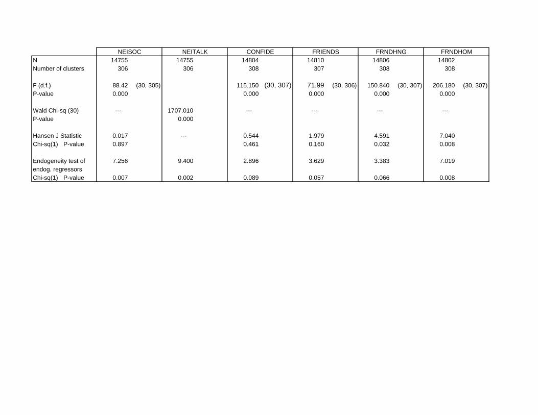
in the west-central part of the country, which corresponds to the Plains states. Finally, the test

for endogeneity of the tract density measure suggest that this variable is indeed endogenous,

and the overidentification J-test shows that the instruments are valid.

Panel B of Table 3 shows IVPROBIT results using the binary NEITALK measure as

dependent variable. This variable, which indicates that the respondent interacts with neighbors

at least once a week, is a less-precise measure than NEISOC. Apparently because of this

difference, the tract-density coefficient, while still negative, is now insignificant. The signs and

significance of the remaining coefficients mostly follow the pattern in panel A, except that none

of the income coefficients is significant. The Wald test rejects exogeneity of tract-density.9

Panel C of the table shows 2SLS results when CONFIDE is the dependent variable. The

tract-density coefficient is negative and significant, indicating that respondents living in dense

census tracts have fewer confidants. Once again, this result contradicts the hypothesis of

stronger interaction in denser areas. While the effects of income, education, minority status,

retirement, and citizenship match those in the NEISOC equation, marriage and children now

have significantly negative coefficients. Apparently, marriage and children increase superficial

contacts with neighbors, but reduce the formation of strong outside bonds by fostering an

inward orientation. While panel A showed that older respondents interact more with their

neighbors, panel C shows they have fewer confidants up to the quadratic minimum of 51

years, beyond which the age effect turns positive. Also, residence outside of the Pacific region

mostly reduces the number of confidants, in contrast to the findings for neighbor interaction.

Finally, male respondents have fewer confidants than do females, and unemployment now has

a significantly negative effect. While the endogeneity test now cannot reject exogeneity of tract

density, the overidentification J-test nevertheless indicates validity of the instruments.

Panel D shows 2SLS results when FRIENDS is the dependent variable. The tract-density

coefficient is again negative and significant, indicating that higher tract density reduces the

number of friends, which again contradicts the main hypothesis. The effects of age, marriage,

children, income, education, minority status, retirement, and unemployment match those in

panel C, but the sex effect is now reversed, with males having more friends than females.10

11

Long-time neighborhood residence shows its first significant impact, raising the number of

friends. The non-Pacific regional coefficients are mostly negative, but residence in the west-

north-central regional raises the number of friends. Both diagnostic tests are satisfactory.

Panel E shows 2SLS results when FRNDHNG is the dependent variable. The tract-density

coefficient, while negative, is now insignificant. The effects of age, marriage, children, income,

education, minority status, retirement, and long-time neighborhood residence match those

in panel D, but the male coefficient is now significantly negative.11 Evidently, while male

respondents have more friends, they spend less time hanging out with them in public places

than do females. Regional impacts are again mixed, but the effect of unemployment is no longer

significant. Exogeneity of tract density is rejected, but the J-test now rejects the overidentifying

restrictions. Therefore, there are grounds for questioning the suitability of the instruments for

this equation, despite their good performance in the other regressions.

Panel F of Table 3 shows 2SLS results when FRNDHOM is the dependent variable. The

tract-density coefficient is again negative but now significant, indicating that respondents invite

friends to their homes less frequently in denser census tracts. The other results mostly match

those in panel E, except that the male coefficient is insignificant.12 The diagnostic tests show

the same pattern as in panel E.

Table 3 also shows the tract-density coefficients when the various equations are estimated

without instrumental variables, using either OLS or regular probit. As can be seen, the density

coefficients are insignificant in the non-IV case in the NEISOC, CONFIDE, FRIENDS, FRND-

HOM equations, becoming significantly negative when IV estimation is used. By contrast, the

non-IV coefficients are significantly positive in the NEITALK and FRNDHNG equations, while

IV estimation leads to coefficients that are negative and insignificant. These comparison sug-

gest that, for each equation, IV methods eliminate an upward bias in the non-IV estimates.

This conclusion, in turn, suggests that tract density is positively correlated with the error term

in each equation, indicating that individuals whose unobservable attributes favor interaction

tend to reside in high-density census tracts. Note that, while this locational tendency is the

one predicted above, the earlier rationale for it is now absent. In other words, since interac-

tion decreases rather than increases with density, interactive individuals sacrifice something by

12

locating in dense tracts and therefore must have another reason to do so.

Note that, while the positive and significant non-IV coefficients in the NEITALK and

FRNDHNG equations would ordinarily be viewed as confirmation of the Putnam hypothesis,

the IV results show that these results are spurious, being the consequence of sorting by in-

dividuals across neighborhoods. In other words, the apparent tendency of interaction-prone

individuals to locate in dense neighborhoods leads to a positive correlation between density and

interaction, as reflected in the non-IV estimates. Controlling for this locational endogeneity,

the IV results show that, if a given individual (with a particular unobservable propensity to

interact) were relocated from a dense to a less dense census tract, the level of interaction for

this person would rise, not fall.

Summing up, the results in Table 3 strongly contradict the main hypothesis, showing that

social interaction tends to be weaker, not stronger, in high-density census tracts. While a

positive density effect might make sense given that people living in close proximity should find

interaction easier, the data disconfirm this logic. Possible reasons for the contrary findings are

discussed in section 4.5 below.

4.3. Results for group-involvement variables

Group involvement measures another dimension of social interaction, and Table 4 presents

results for the four variables in this set. Panel A of the table shows IVPROBIT results with

NEICOOP as the dependent variable. Note that, because of a large number of missing NE-

ICOOP values, the sample size for this estimation is only 7316. The tract-density variable is

positive but insignificant, indicating no effect of density on the likelihood of cooperating with

neighbors. But cooperation increases with age, marriage, the presence of children, income,

education, citizenship, long-time residence, and the respondent’s status as a homemaker.13

Interestingly, black respondents are more likely to cooperate with neighbors than non-minority

households, although the Hispanic and Asian coefficients are insignificant. Cooperation tends

to be more likely outside the Pacific region. The Wald test cannot reject exogeneity of tract

density.14

Panel B of Table 4 shows IVPROBIT results with GRPHOB as the dependent variable.

The tract density coefficient is significantly negative, indicating that membership in a hobby-

13

oriented club is less likely in a dense census tract. This finding again contradicts the main

hypothesis. Club membership is higher for males and rises with age, income, education, retire-

ment and citizenship, but falls with marriage and the presence of children.15 The coefficients

of the race and regional variables are now uniformly insignificant. Exogeneity of tract density

is rejected by the Wald test.16

Panel C shows 2SLS results with CCLUBMET as the dependent variable. The tract-

density coefficient is again negative, indicating that respondents living in dense census tracts

attend relatively few club meetings, again contradicting the main hypothesis. While the effects

of income, education, marriage, the presence of young children, education, retirement, and

citizenship are the same as in panel B, the presence of older children raises the frequency of

club attendance (perhaps a Boy Scout effect). In addition, males attend fewer meetings, age

and unemployment now have negative impacts, and long-time residence has a positive effect.17

Regional effects remain absent, and the diagnostic tests are satisfactory.

Panel D shows 2SLS results with GPRINVLV as the dependent variable. A negative

coefficient again emerges for tract density, showing that respondents in dense areas belong to

relatively few non-church groups. While the effects of income, education, the presence of older

children, and citizenship remain the same, the results show higher group membership for black

and Hispanic respondents and lower membership for Asians. Given the insignificant racial

effects for hobby-oriented club membership, this effect is apparently capturing membership

effects for other types of groups. Respondents who are unemployed or are homemakers also

belong to fewer groups, while sex, marriage, young children, and long-time residence have no

effect. Regional effects are again absent, and the diagnostic tests are satisfactory.

Table 4 again shows the tract-density coefficients from non-IV regressions, and they mostly

show the same pattern as in Table 3. In particular, the non-IV GRPHOB, CCLUBMET,

GRPINVLV density coefficients are all insignificant, while IV estimation leads to coefficients

that are significantly negative. Although both NEICOOP density coefficients are insignificant,

these other results suggest that IV estimation tends to eliminate an upward bias in the non-IV

coefficients, indicating a positive correlation between tract density and the error term.

Summing up, the estimates provide the same message as the results for the friendship-

14

oriented interaction measures. Group involvement tends to be weaker, not stronger, in high-

density census tracts, contradicting the main hypothesis.

4.4. Results for other specifications

Table 5 shows the estimated tract-density coefficients for two additional specifications.

The first column shows the consequences of dropping average MSA density as an instrumental

variable, using urbanized-area density as a single instrument. By comparison with the results

in Tables 3 and 4, it can be seen that, with the exception of the FRIENDS density coefficient,

which is only significant at the 10 percent level, the set of significant coefficients is unaffected

by use of the single instrument. In addition, the magnitudes of most density coefficients change

only slightly, although the FRNDHNG and FRNDHOM coefficients show nontrivial changes.

The coefficients for the other covariates, which are not reported, exhibit little change between

the two specifications.

The second column of Table 5 shows the consequences of dropping PART MAR, HOME-

MAKER and the KIDS variables as covariates, on the grounds of potential endogeneity. While

the coefficient signs remain the same, estimated magnitudes show more-substantial changes

than in column one, and two previously significant density coefficients (in the CONFIDE and

FRIENDS equations) now are significant only at the 10 percent level. However, the previ-

ously insignificant NEITALK coefficient is now nearly significant at the 5 percent level. The

estimate coefficients for most of the other covariates are not greatly affected by this change in

specification.

Overall, the results in Table 5 show that the main finding of the paper, density’s negative

effect on interaction, is reasonably robust to these two changes in the specification of the model.

In addition to considering these other specifications, it is useful to compare the present

results to selected findings from Gottlieb and Glaeser (2006) and Borck (2006). These papers

focus on broad sets of social-capital measures, but a few of their regressions involve social-

interaction measures like the present ones. Using a survey variable indicating whether the

respondent entertains friends at home, Glaeser and Gottlieb (2006) present a regression showing

that such behavior is less likely in cities than in suburbs. However, this result, which is

consistent with present findings, disappears in regressions for the period after 1990. Borck’s

15

results show that a survey respondent’s number of friends is unaffected by city size, while the

level of interaction with friends is greater in large cities. With a positive correlation between

density and city size, this latter result appears to contradict the present findings.18

4.5. Why is the density effect negative?

The paper’s maintained hypothesis, that social interaction is stronger in denser areas, arose

from the conjecture that high densities facilitate interaction by putting people in close prox-

imity. The results, however, show the opposite effect, and a question is why. One possibility

is that dense environments offer residents more sources of entertainment (museums, theaters,

etc.), lessening the need to interact with others in the pursuit of stimulation.19 Alternatively,

the crowding associated with a dense environment might spur a need for privacy, causing

people to draw inward. Such behavior could reflect the old saying: “good fences make good

neighbors.” Another possibility is that high densities may be associated with criminal activity,

making people suspicious of one another and reluctant to interact.

The latter conjecture might be testable by including a crime measure in the interaction

equation along with density. Comprehensive crime data are not available at the census tract

level, but even if they were, the tract crime level must be viewed as endogenous in the same

fashion as density (being the result of household’s locational choice). As a result, evaluating

crime as a root cause of the density effect is not at all straightforward.

Since crime may limit interaction by eroding trust between individuals, an alternative ap-

proach would be to include the survey’s trust variable as a covariate in the regression along

with density (the variable measures the degree of trust that the respondent feels toward oth-

ers). However, this approach is also problematic. The difficulty is that trust is endogenous,

presumably being dependent on life experiences such as crime victimization, which in turn

may be a function of density. As a result, trust seems inappropriate as an additional covariate

in an equation explaining interaction.

Given this discussion, it appears that isolating the root cause of the negative density effect

is a difficult task, one that is beyond the scope of the present paper. Indeed, the message

of this paper would be unaffected by the results of any such further inquiry. Whatever the

reason, density has been shown to exert a negative influence on social interaction, undermining

16

an important line of attack used by critics of urban sprawl.

5. Conclusion

Various authors, most notably Putnam (2000), have argued that low-density living reduces

social interaction, and this argument has been used to buttress criticisms of urban sprawl. But

urban expansion must involve market failures if it is to be inefficient, and this paper shows that

such a distortion indeed arises if low density depresses social interaction. Then, in appraising

the gains from greater individual consumption of living space, consumers fail to consider re-

duced interaction benefits for their neighbors, which arise through lower neighborhood density.

Space consumption is then too high, and cities are excessively spread out.

The key element in this argument is a positive link between social interaction and neigh-

borhood density, and the paper tests empirically for such a link. The results are unfavorable:

whether the focus is friendship-oriented social interaction or measures of group involvement,

the empirical results show a negative, rather than positive, effect of density on interaction.

The paper’s findings therefore imply that social-interaction effects cannot be credibly in-

cluded in the panoply of criticisms directed toward urban sprawl. In fact, the results suggest

an opposite line of argument. With a negative effect of density on interaction, individual space

consumption would tend to be too low rather than too high, tending to make cities inefficiently

compact, as explained in section 2. Thus, the empirical results suggest that social-interaction

effects may counteract, rather than exacerbate, the well-recognized forces (such as unpriced

traffic congestion) that cause cities to overexpand.

17

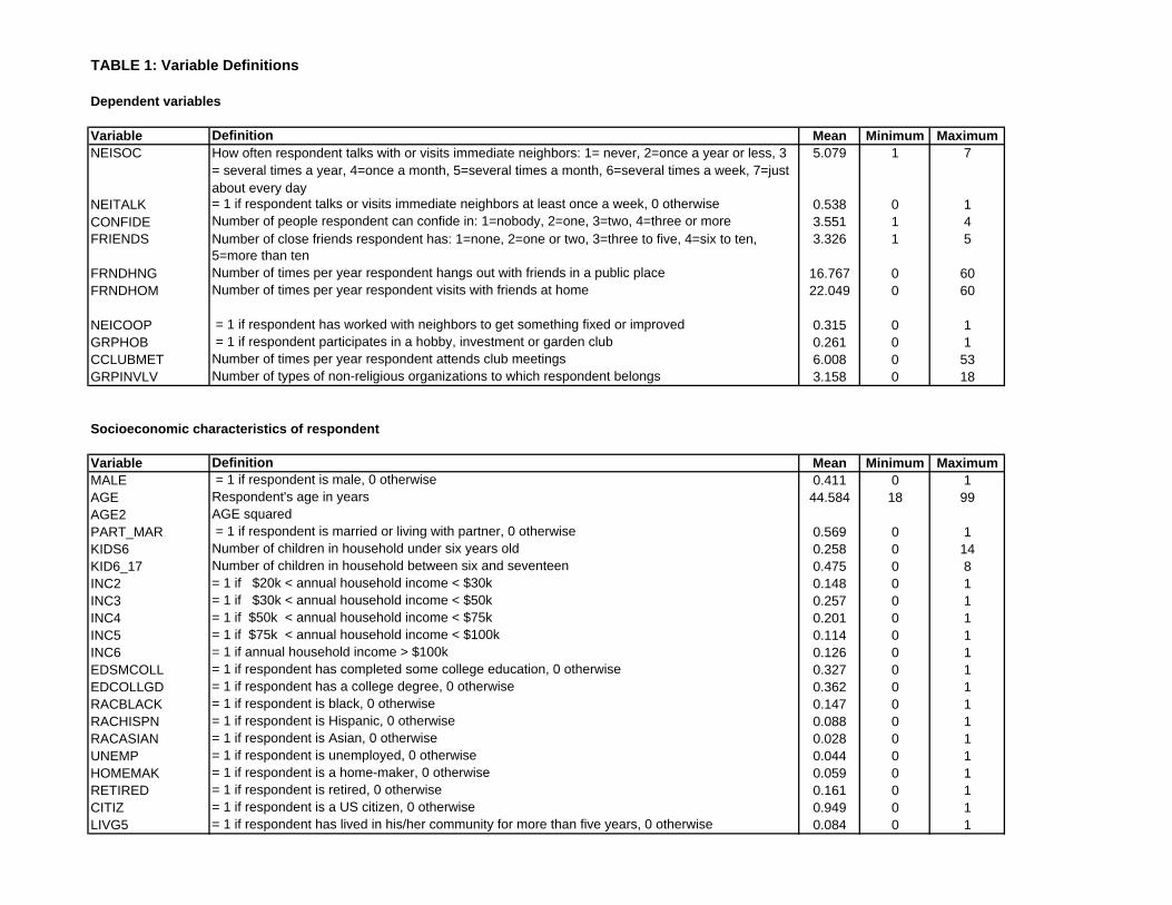
TABLE 1: Variable Definitions

Dependent variables

Variable Definition Mean Minimum MaximumNEISOC How often respondent talks with or visits immediate neighbors: 1= never, 2=once a year or less, 3

= several times a year, 4=once a month, 5=several times a month, 6=several times a week, 7=just about every day

5.079 1 7

NEITALK = 1 if respondent talks or visits immediate neighbors at least once a week, 0 otherwise 0.538 0 1CONFIDE Number of people respondent can confide in: 1=nobody, 2=one, 3=two, 4=three or more 3.551 1 4FRIENDS Number of close friends respondent has: 1=none, 2=one or two, 3=three to five, 4=six to ten,

5=more than ten3.326 1 5

FRNDHNG Number of times per year respondent hangs out with friends in a public place 16.767 0 60FRNDHOM Number of times per year respondent visits with friends at home 22.049 0 60

NEICOOP = 1 if respondent has worked with neighbors to get something fixed or improved 0.315 0 1GRPHOB = 1 if respondent participates in a hobby, investment or garden club 0.261 0 1CCLUBMET Number of times per year respondent attends club meetings 6.008 0 53GRPINVLV Number of types of non-religious organizations to which respondent belongs 3.158 0 18

Socioeconomic characteristics of respondent

Variable Definition Mean Minimum MaximumMALE = 1 if respondent is male, 0 otherwise 0.411 0 1AGE Respondent's age in years 44.584 18 99AGE2 AGE squaredPART_MAR = 1 if respondent is married or living with partner, 0 otherwise 0.569 0 1KIDS6 Number of children in household under six years old 0.258 0 14KID6_17 Number of children in household between six and seventeen 0.475 0 8INC2 = 1 if $20k < annual household income < $30k 0.148 0 1INC3 = 1 if $30k < annual household income < $50k 0.257 0 1INC4 = 1 if $50k < annual household income < $75k 0.201 0 1INC5 = 1 if $75k < annual household income < $100k 0.114 0 1INC6 = 1 if annual household income > $100k 0.126 0 1EDSMCOLL = 1 if respondent has completed some college education, 0 otherwise 0.327 0 1EDCOLLGD = 1 if respondent has a college degree, 0 otherwise 0.362 0 1RACBLACK = 1 if respondent is black, 0 otherwise 0.147 0 1RACHISPN = 1 if respondent is Hispanic, 0 otherwise 0.088 0 1RACASIAN = 1 if respondent is Asian, 0 otherwise 0.028 0 1UNEMP = 1 if respondent is unemployed, 0 otherwise 0.044 0 1HOMEMAK = 1 if respondent is a home-maker, 0 otherwise 0.059 0 1RETIRED = 1 if respondent is retired, 0 otherwise 0.161 0 1CITIZ = 1 if respondent is a US citizen, 0 otherwise 0.949 0 1LIVG5 = 1 if respondent has lived in his/her community for more than five years, 0 otherwise 0.084 0 1

Population density measures

Variable Definition Mean Minimum MaximumLNPDEN_TRACT Census tract density: people per square mile 8.008 1.529 12.258LNPDEN_UA Urbanized Area density: people per square mile 7.845 6.747 8.863LNPDEN_P_MSA MSA density: people per square mile 6.188 3.281 7.615

Regional controls. Omitted category: Pacific

Variable Definition Mean Minimum MaximumNEWENGL =1 if census region is New England, 0 otherwise 0.066 0 1MIDATLAN =1 if census region is Mid Atlantic, 0 otherwise 0.096 0 1EANOCENT =1 if census region is East North Central, 0 otherwise 0.247 0 1WENOCENT =1 if census region is West North Central, 0 otherwise 0.060 0 1SOUTHATL =1 if census region is South Atlantic, 0 otherwise 0.206 0 1EASOCENT =1 if census region is East South Central, 0 otherwise 0.044 0 1WESOCENT =1 if census region is West South Central, 0 otherwise 0.030 0 1MOUNTN =1 if census region is Mountain, 0 otherwise 0.078 0 1

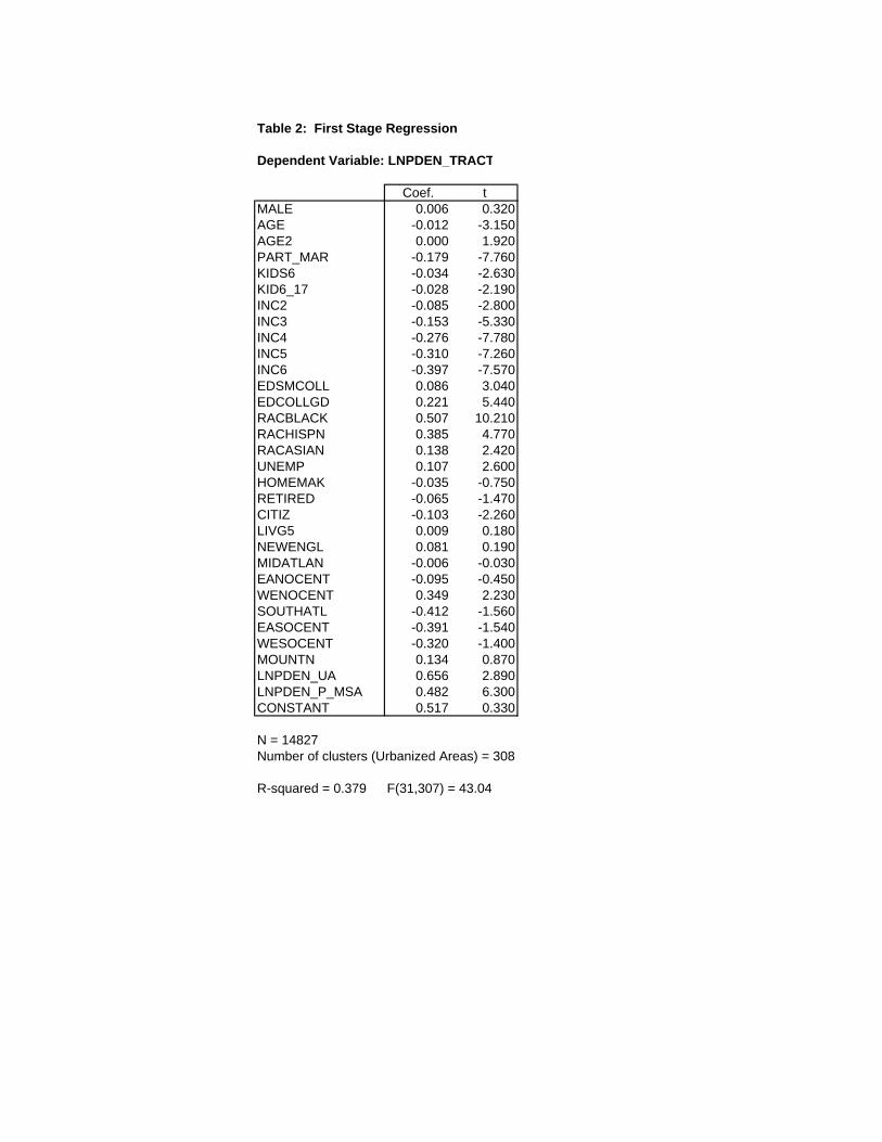
Table 2: First Stage Regression

Dependent Variable: LNPDEN_TRACT

Coef. tMALE 0.006 0.320AGE -0.012 -3.150AGE2 0.000 1.920PART_MAR -0.179 -7.760KIDS6 -0.034 -2.630KID6_17 -0.028 -2.190INC2 -0.085 -2.800INC3 -0.153 -5.330INC4 -0.276 -7.780INC5 -0.310 -7.260INC6 -0.397 -7.570EDSMCOLL 0.086 3.040EDCOLLGD 0.221 5.440RACBLACK 0.507 10.210RACHISPN 0.385 4.770RACASIAN 0.138 2.420UNEMP 0.107 2.600HOMEMAK -0.035 -0.750RETIRED -0.065 -1.470CITIZ -0.103 -2.260LIVG5 0.009 0.180NEWENGL 0.081 0.190MIDATLAN -0.006 -0.030EANOCENT -0.095 -0.450WENOCENT 0.349 2.230SOUTHATL -0.412 -1.560EASOCENT -0.391 -1.540WESOCENT -0.320 -1.400MOUNTN 0.134 0.870LNPDEN_UA 0.656 2.890LNPDEN_P_MSA 0.482 6.300CONSTANT 0.517 0.330

N = 14827Number of clusters (Urbanized Areas) = 308

R-squared = 0.379 F(31,307) = 43.04

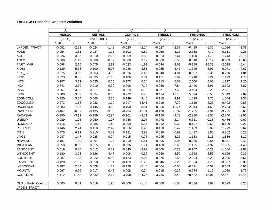
TABLE 3: Friendship-Oriented Variables

Coeff z Coeff z Coeff z Coeff z Coeff z Coeff zLNPDEN_TRACT -0.081 -2.51 -0.024 -1.48 -0.020 -2.14 -0.027 -2.37 -0.419 -1.36 -1.086 -3.38MALE 0.054 1.61 0.027 1.13 -0.102 -9.50 0.060 3.27 -2.358 -7.79 0.111 0.36AGE 0.024 3.35 0.010 2.10 -0.009 -3.80 -0.023 -6.41 -1.400 -21.73 -1.243 -20.76AGE2 0.000 -1.13 0.000 -0.07 0.000 3.17 0.000 6.53 0.010 15.12 0.009 13.63PART_MAR 0.098 2.75 0.075 2.92 -0.023 -1.91 -0.044 -2.62 -5.299 -15.39 -2.035 -5.44KIDS6 0.129 5.68 0.100 5.07 -0.036 -3.81 -0.055 -3.47 -1.649 -5.91 -0.971 -4.67KID6_17 0.075 3.59 0.053 4.09 -0.026 -3.46 -0.048 -4.81 -0.907 -5.33 -0.280 -1.04INC2 0.023 0.36 -0.035 -1.13 0.106 3.84 0.131 3.97 1.218 2.24 1.129 1.78INC3 0.207 3.72 0.025 0.66 0.173 6.24 0.213 6.68 2.500 5.08 1.877 3.20INC4 0.241 3.70 0.010 0.30 0.206 7.19 0.256 7.84 3.440 5.91 2.602 3.87INC5 0.257 3.55 0.011 0.23 0.219 8.10 0.271 7.58 4.404 6.23 2.591 3.10INC6 0.280 3.62 0.034 0.63 0.272 8.48 0.414 11.18 5.694 8.55 5.049 7.07EDSMCOLL 0.120 3.04 0.065 2.85 0.149 9.46 0.115 4.91 1.699 4.75 1.044 2.36EDCOLLGD 0.072 1.63 -0.033 -1.10 0.217 14.41 0.219 7.79 1.119 2.23 -0.402 -0.85RACBLACK -0.383 -7.05 -0.145 -4.12 -0.190 -8.81 -0.386 -12.74 -2.044 -4.69 -2.783 -5.62RACHISPN -0.467 -6.37 -0.195 -3.83 -0.294 -11.31 -0.198 -5.32 -1.285 -1.91 -3.725 -5.63RACASIAN -0.290 -3.11 -0.159 -2.94 -0.161 -3.71 -0.159 -3.73 -2.280 -3.56 -2.740 -2.90UNEMP -0.089 -1.03 -0.050 -1.07 -0.056 -2.08 -0.078 -2.14 -0.311 -0.35 0.486 0.60HOMEMAK 0.116 1.49 0.085 1.42 0.009 0.36 0.012 0.30 0.407 0.63 0.129 0.21RETIRED 0.146 2.24 0.110 2.47 0.016 0.48 0.120 3.42 1.463 2.09 1.773 2.62CITIZ 0.475 6.11 0.310 5.72 0.121 2.93 0.036 0.92 1.437 1.85 4.202 6.28LIVG5 0.087 1.47 0.028 0.74 -0.015 -0.77 0.095 3.27 1.183 2.13 1.886 3.17NEWENGL -0.181 -1.59 -0.091 -1.27 -0.010 -0.61 -0.096 -3.95 -0.335 -0.54 0.351 0.42MIDATLAN -0.050 -0.63 0.015 0.30 -0.096 -5.74 -0.108 -3.65 -1.165 -1.97 -1.355 -1.48EANOCENT 0.019 0.35 0.012 0.32 -0.045 -2.93 -0.006 -0.23 -0.107 -0.21 -1.556 -2.83WENOCENT 0.180 3.23 0.126 4.47 -0.008 -0.36 0.066 2.59 1.668 2.55 0.166 0.36SOUTHATL -0.087 -1.33 -0.022 -0.53 -0.123 -6.05 -0.076 -2.55 -2.294 -3.22 -3.095 -5.61EASOCENT -0.120 -1.37 -0.058 -1.04 -0.169 -5.23 -0.046 -1.26 -1.364 -1.78 -3.067 -3.30WESOCENT 0.187 2.84 0.078 1.73 -0.129 -5.46 -0.004 -0.08 -0.311 -0.52 0.609 0.93MOUNTN 0.097 0.99 0.017 0.45 -0.008 -0.34 0.015 0.32 0.784 1.12 1.039 1.75CONSTANT 4.112 11.43 -0.532 -2.64 3.708 34.76 3.736 28.40 60.422 18.01 62.561 19.46

OLS or Probit Coeff, z 0.005 0.31 0.019 1.96 -0.006 -1.46 -0.006 -1.03 0.334 2.67 0.029 0.20LPDEN_TRACT

FRNDHOMFRNDHNGFRIENDSCONFIDENEITALKNEISOCA B

(2SLS) (IVPROBIT)

C D E F

(2SLS) (2SLS) (2SLS) (2SLS)

N 14755 14755 14804 14810 14806 14802Number of clusters 306 306 308 307 308 308

F (d.f.) 88.42 (30, 305) 115.150 (30, 307) 71.99 (30, 306) 150.840 (30, 307) 206.180 (30, 307)P-value 0.000 0.000 0.000 0.000 0.000

Wald Chi-sq (30) --- 1707.010 --- --- --- ---P-value 0.000

Hansen J Statistic 0.017 --- 0.544 1.979 4.591 7.040Chi-sq(1) P-value 0.897 0.461 0.160 0.032 0.008

Endogeneity test of 7.256 9.400 2.896 3.629 3.383 7.019endog. regressorsChi-sq(1) P-value 0.007 0.002 0.089 0.057 0.066 0.008

NEISOC NEITALK CONFIDE FRIENDS FRNDHNG FRNDHOM

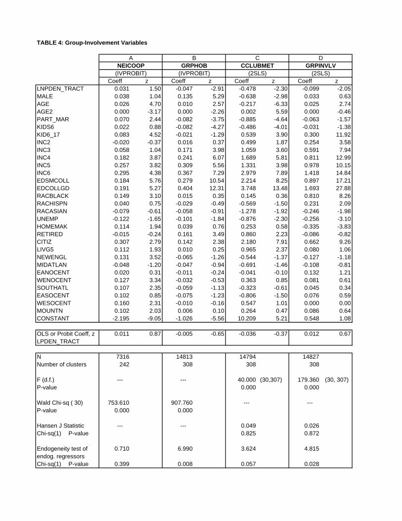
TABLE 4: Group-Involvement Variables

Coeff z Coeff z Coeff z Coeff zLNPDEN_TRACT 0.031 1.50 -0.047 -2.91 -0.478 -2.30 -0.099 -2.05MALE 0.038 1.04 0.135 5.29 -0.638 -2.98 0.033 0.63AGE 0.026 4.70 0.010 2.57 -0.217 -6.33 0.025 2.74AGE2 0.000 -3.17 0.000 -2.26 0.002 5.59 0.000 -0.46PART_MAR 0.070 2.44 -0.082 -3.75 -0.885 -4.64 -0.063 -1.57KIDS6 0.022 0.88 -0.082 -4.27 -0.486 -4.01 -0.031 -1.38KID6_17 0.083 4.52 -0.021 -1.29 0.539 3.90 0.300 11.92INC2 -0.020 -0.37 0.016 0.37 0.499 1.87 0.254 3.58INC3 0.058 1.04 0.171 3.98 1.059 3.60 0.591 7.94INC4 0.182 3.87 0.241 6.07 1.689 5.81 0.811 12.99INC5 0.257 3.82 0.309 5.56 1.331 3.98 0.978 10.15INC6 0.295 4.38 0.367 7.29 2.979 7.89 1.418 14.84EDSMCOLL 0.184 5.76 0.279 10.54 2.214 8.25 0.897 17.21EDCOLLGD 0.191 5.27 0.404 12.31 3.748 13.48 1.693 27.88RACBLACK 0.149 3.10 0.015 0.35 0.145 0.36 0.810 8.26RACHISPN 0.040 0.75 -0.029 -0.49 -0.569 -1.50 0.231 2.09RACASIAN -0.079 -0.61 -0.058 -0.91 -1.278 -1.92 -0.246 -1.98UNEMP -0.122 -1.65 -0.101 -1.84 -0.876 -2.30 -0.256 -3.10HOMEMAK 0.114 1.94 0.039 0.76 0.253 0.58 -0.335 -3.83RETIRED -0.015 -0.24 0.161 3.49 0.860 2.23 -0.086 -0.82CITIZ 0.307 2.79 0.142 2.38 2.180 7.91 0.662 9.26LIVG5 0.112 1.93 0.010 0.25 0.965 2.37 0.080 1.06NEWENGL 0.131 3.52 -0.065 -1.26 -0.544 -1.37 -0.127 -1.18MIDATLAN -0.048 -1.20 -0.047 -0.94 -0.691 -1.46 -0.108 -0.81EANOCENT 0.020 0.31 -0.011 -0.24 -0.041 -0.10 0.132 1.21WENOCENT 0.127 3.34 -0.032 -0.53 0.363 0.85 0.081 0.61SOUTHATL 0.107 2.35 -0.059 -1.13 -0.323 -0.61 0.045 0.34EASOCENT 0.102 0.85 -0.075 -1.23 -0.806 -1.50 0.076 0.59WESOCENT 0.160 2.31 -0.010 -0.16 0.547 1.01 0.000 0.00MOUNTN 0.102 2.03 0.006 0.10 0.264 0.47 0.086 0.64CONSTANT -2.195 -9.05 -1.026 -5.56 10.209 5.21 0.548 1.08

OLS or Probit Coeff, z 0.011 0.87 -0.005 -0.65 -0.036 -0.37 0.012 0.67LPDEN_TRACT

N 7316 14813 14794 14827Number of clusters 242 308 308 308

F (d.f.) --- --- 40.000 (30,307) 179.360 (30, 307)P-value 0.000 0.000

Wald Chi-sq ( 30) 753.610 907.760 --- ---P-value 0.000 0.000

Hansen J Statistic --- --- 0.049 0.026Chi-sq(1) P-value 0.825 0.872

Endogeneity test of 0.710 6.990 3.624 4.815endog. regressorsChi-sq(1) P-value 0.399 0.008 0.057 0.028

(IVPROBIT) (IVPROBIT) (2SLS) (2SLS)

A B C DNEICOOP GRPHOB CCLUBMET GRPINVLV

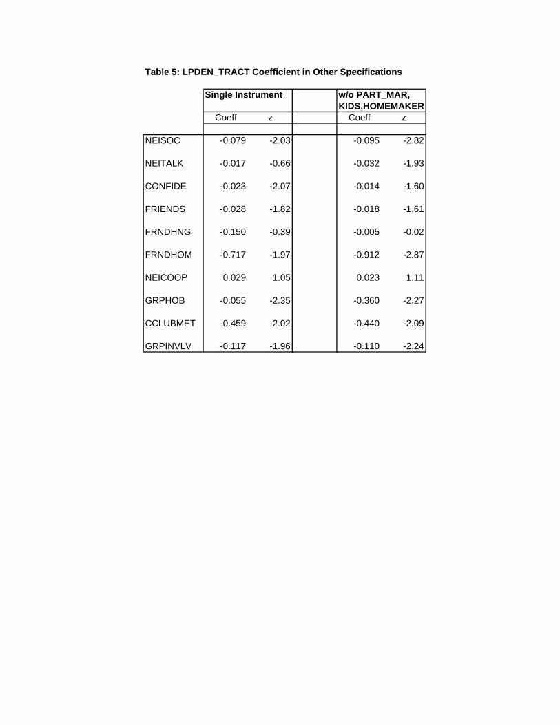
Table 5: LPDEN_TRACT Coefficient in Other Specifications

Single Instrument w/o PART_MAR,KIDS,HOMEMAKER

Coeff z Coeff z

NEISOC -0.079 -2.03 -0.095 -2.82

NEITALK -0.017 -0.66 -0.032 -1.93

CONFIDE -0.023 -2.07 -0.014 -1.60

FRIENDS -0.028 -1.82 -0.018 -1.61

FRNDHNG -0.150 -0.39 -0.005 -0.02

FRNDHOM -0.717 -1.97 -0.912 -2.87

NEICOOP 0.029 1.05 0.023 1.11

GRPHOB -0.055 -2.35 -0.360 -2.27

CCLUBMET -0.459 -2.02 -0.440 -2.09

GRPINVLV -0.117 -1.96 -0.110 -2.24

References

Borck, R., 2006. Social agglomeration externalities. Unpublished paper, DIW Berlin.

Brueckner, J.K., 2000. Urban sprawl: Diagnosis and remedies. International RegionalScience Review 23, 160-171.

Brueckner, J.K., 2001. Urban sprawl: Lessons from urban economics. In: Gale, W.G.,Pack, J.R. (Eds.), Brookings-Wharton Papers on Urban Affairs, Brookings Institution,Washington, D.C., pp. 65-89.

Brueckner, J.K., 2006. Urban growth boundaries: An effective second-best remedy forunpriced road congestion? Unpublished paper, University of California, Irvine.

Ewing, R., Schmid, T., Killingsworth R., Zlot A., Raudenbush, S., 2003. Relation-ship between urban sprawl and physical activity, obesity and morbidity, American Journalof Health Promotion 18, 47-57.

Fujita, M., 1989. Urban Economic Theory, Cambridge University Press, New York.

Glaeser, E.L., Kahn, M.E., 2004. Sprawl and urban growth. In: Henderson, J.V., Thisse,J.-F. (Eds.), Handbook of Urban Economics, Vol. IV, Elsevier, Amsterdam, forthcoming.

Glaeser, E.L., Gottlieb, J.D., 2006. Urban resurgence and the consumer city, UrbanStudies, forthcoming.

Lopez, R., 2004. Urban sprawl and the risk for being overweight or obese, American Journalof Public Health 94, 1574-1579.

Nechyba, T.J., Walsh, R., 2004. Urban sprawl. Journal of Economic Perspectives 18(4),177-200.

Powdthavee, N., 2005. Identifying causal effects with panel data: The case of friendshipand happiness, Unpublished paper, University of London.

Putnam, R.D., 2000. Bowling Alone, Simon and Schuster, New York.

18

Footnotes

∗We thank Rainald Borck, Ami Glazer, David Neumark, Stuart Rosenthal and Ken Small forhelpful comments. They are not responsible, however, for any shortcomings in the paper.

1For a good overview of these arguments, see the 12-article symposium published in the Fall1998 issue of the Brookings Review.

2A properly-set UGB is equivalent to a tax in dealing with the first failure. However, Brueck-ner (2006) shows that a UGB is a poor second-best instrument for dealing with unpricedroad congestion.

3See Powdthavee (2005) for evidence showing that friendships increase happiness.

4A potential connection between urban sprawl and obesity, which is thought to arise fromhigh auto usage and thus low exercise in sprawling cities, has been the focus of a numberof recent papers (see Ewing et al. (2003) and Lopez (2004)). However, even if low-densityliving contributes to obesity, there appears to be no externality involved and thus no basisfor claiming that the effect contributes to an inefficient spatial expansion of cities.

5In providing sensitivity analysis in his regressions relating social capital to city size, Borck(2006) presents IV results that treat city size as endogenous. His instrument is lagged citysize.

6Interaction may have social value as well as generating private benefits. For example, inter-action may insure the beneficial spread of information or foster socially responsible behavior.In this case, the average level of interaction in the city could enter individual i’s utility func-tion along with Ii. However, since interaction is constant across people under the aboveassumptions, this modification would have no effect on the model.

7In Fujita’s model, the density effect arises from the negative environmental impact of crowd-ing.

8Since the equation predicting tract density is estimated jointly with the interaction equationin the maximum likelihood IVPROBIT routine, the coefficients and standard errors differslightly from those in Table 2.

9To test for validity of the instruments, the probit equation was reestimated as a linear

19

probability model using 2SLS. The J-test failed to reject the overidentifying restrictions.

10The age effect turns positive beyond the quadratic minimum at 44 years.

11The age effect turns positive beyond 69 years.

12The age effect turns positive beyond 69 years.

13The age effect turns negative beyond 67 years.

14In a 2SLS linear probability model, the J-test did not reject the overidentifying restrictions.

15The age effect turns negative beyond 51 years.

16In a 2SLS linear probability model, the J-test did not reject the overidentifying restrictions.

17The age effect turns positive beyond 53 years.

18Glaeser and Gottlieb’s study relies on the DDB Needham Life Style Survey, while Borck’suses data from the German Socio-Economic Panel.

19Glaeser and Gottlieb (2006) present results showing how participation in various outsideentertainment activities is greater in central cities than in suburbs.

20

CESifo Working Paper Series (for full list see Twww.cesifo-group.de)T

___________________________________________________________________________ 1780 Gregory Ponthiere, Growth, Longevity and Public Policy, August 2006 1781 Laszlo Goerke, Corporate and Personal Income Tax Declarations, August 2006 1782 Florian Englmaier, Pablo Guillén, Loreto Llorente, Sander Onderstal and Rupert

Sausgruber, The Chopstick Auction: A Study of the Exposure Problem in Multi-Unit Auctions, August 2006

1783 Adam S. Posen and Daniel Popov Gould, Has EMU had any Impact on the Degree of

Wage Restraint?, August 2006 1784 Paolo M. Panteghini, A Simple Explanation for the Unfavorable Tax Treatment of

Investment Costs, August 2006 1785 Alan J. Auerbach, Why have Corporate Tax Revenues Declined? Another Look, August

2006 1786 Hideshi Itoh and Hodaka Morita, Formal Contracts, Relational Contracts, and the

Holdup Problem, August 2006 1787 Rafael Lalive and Alejandra Cattaneo, Social Interactions and Schooling Decisions,

August 2006 1788 George Kapetanios, M. Hashem Pesaran and Takashi Yamagata, Panels with

Nonstationary Multifactor Error Structures, August 2006 1789 Torben M. Andersen, Increasing Longevity and Social Security Reforms, August 2006 1790 John Whalley, Recent Regional Agreements: Why so many, why so much Variance in

Form, why Coming so fast, and where are they Headed?, August 2006 1791 Sebastian G. Kessing and Kai A. Konrad, Time Consistency and Bureaucratic Budget

Competition, August 2006 1792 Bertil Holmlund, Qian Liu and Oskar Nordström Skans, Mind the Gap? Estimating the

Effects of Postponing Higher Education, August 2006 1793 Peter Birch Sørensen, Can Capital Income Taxes Survive? And Should They?, August

2006 1794 Michael Kosfeld, Akira Okada and Arno Riedl, Institution Formation in Public Goods

Games, September 2006 1795 Marcel Gérard, Reforming the Taxation of Multijurisdictional Enterprises in Europe, a

Tentative Appraisal, September 2006

1796 Louis Eeckhoudt, Béatrice Rey and Harris Schlesinger, A Good Sign for Multivariate

Risk Taking, September 2006 1797 Dominique M. Gross and Nicolas Schmitt, Why do Low- and High-Skill Workers

Migrate? Flow Evidence from France, September 2006 1798 Dan Bernhardt, Stefan Krasa and Mattias Polborn, Political Polarization and the

Electoral Effects of Media Bias, September 2006 1799 Pierre Pestieau and Motohiro Sato, Estate Taxation with Both Accidental and Planned

Bequests, September 2006 1800 Øystein Foros and Hans Jarle Kind, Do Slotting Allowances Harm Retail Competition?,

September 2006 1801 Tobias Lindhe and Jan Södersten, The Equity Trap, the Cost of Capital and the Firm’s

Growth Path, September 2006 1802 Wolfgang Buchholz, Richard Cornes and Wolfgang Peters, Existence, Uniqueness and

Some Comparative Statics for Ratio- and Lindahl Equilibria: New Wine in Old Bottles, September 2006

1803 Jan Schnellenbach, Lars P. Feld and Christoph Schaltegger, The Impact of Referendums

on the Centralisation of Public Goods Provision: A Political Economy Approach, September 2006

1804 David-Jan Jansen and Jakob de Haan, Does ECB Communication Help in Predicting its

Interest Rate Decisions?, September 2006 1805 Jerome L. Stein, United States Current Account Deficits: A Stochastic Optimal Control

Analysis, September 2006 1806 Friedrich Schneider, Shadow Economies and Corruption all over the World: What do

we really Know?, September 2006 1807 Joerg Lingens and Klaus Waelde, Pareto-Improving Unemployment Policies,

September 2006 1808 Axel Dreher, Jan-Egbert Sturm and James Raymond Vreeland, Does Membership on

the UN Security Council Influence IMF Decisions? Evidence from Panel Data, September 2006

1809 Prabir De, Regional Trade in Northeast Asia: Why do Trade Costs Matter?, September

2006 1810 Antonis Adam and Thomas Moutos, A Politico-Economic Analysis of Minimum Wages

and Wage Subsidies, September 2006 1811 Guglielmo Maria Caporale and Christoph Hanck, Cointegration Tests of PPP: Do they

also Exhibit Erratic Behaviour?, September 2006

1812 Robert S. Chirinko and Hisham Foad, Noise vs. News in Equity Returns, September

2006 1813 Oliver Huelsewig, Eric Mayer and Timo Wollmershaeuser, Bank Behavior and the Cost

Channel of Monetary Transmission, September 2006 1814 Michael S. Michael, Are Migration Policies that Induce Skilled (Unskilled) Migration

Beneficial (Harmful) for the Host Country?, September 2006 1815 Eytan Sheshinski, Optimum Commodity Taxation in Pooling Equilibria, October 2006 1816 Gottfried Haber and Reinhard Neck, Sustainability of Austrian Public Debt: A Political

Economy Perspective, October 2006 1817 Thiess Buettner, Michael Overesch, Ulrich Schreiber and Georg Wamser, The Impact of

Thin-Capitalization Rules on Multinationals’ Financing and Investment Decisions, October 2006

1818 Eric O’N. Fisher and Sharon L. May, Relativity in Trade Theory: Towards a Solution to

the Mystery of Missing Trade, October 2006 1819 Junichi Minagawa and Thorsten Upmann, Labor Supply and the Demand for Child

Care: An Intertemporal Approach, October 2006 1820 Jan K. Brueckner and Raquel Girvin, Airport Noise Regulation, Airline Service Quality,

and Social Welfare, October 2006 1821 Sijbren Cnossen, Alcohol Taxation and Regulation in the European Union, October

2006 1822 Frederick van der Ploeg, Sustainable Social Spending in a Greying Economy with

Stagnant Public Services: Baumol’s Cost Disease Revisited, October 2006 1823 Steven Brakman, Harry Garretsen and Charles van Marrewijk, Cross-Border Mergers &

Acquisitions: The Facts as a Guide for International Economics, October 2006 1824 J. Atsu Amegashie, A Psychological Game with Interdependent Preference Types,

October 2006 1825 Kurt R. Brekke, Ingrid Koenigbauer and Odd Rune Straume, Reference Pricing of

Pharmaceuticals, October 2006 1826 Sean Holly, M. Hashem Pesaran and Takashi Yamagata, A Spatio-Temporal Model of

House Prices in the US, October 2006 1827 Margarita Katsimi and Thomas Moutos, Inequality and the US Import Demand

Function, October 2006 1828 Eytan Sheshinski, Longevity and Aggregate Savings, October 2006

1829 Momi Dahan and Udi Nisan, Low Take-up Rates: The Role of Information, October

2006 1830 Dieter Urban, Multilateral Investment Agreement in a Political Equilibrium, October

2006 1831 Jan Bouckaert and Hans Degryse, Opt In Versus Opt Out: A Free-Entry Analysis of

Privacy Policies, October 2006 1832 Wolfram F. Richter, Taxing Human Capital Efficiently: The Double Dividend of

Taxing Non-qualified Labour more Heavily than Qualified Labour, October 2006 1833 Alberto Chong and Mark Gradstein, Who’s Afraid of Foreign Aid? The Donors’

Perspective, October 2006 1834 Dirk Schindler, Optimal Income Taxation with a Risky Asset – The Triple Income Tax,

October 2006 1835 Andy Snell and Jonathan P. Thomas, Labour Contracts, Equal Treatment and Wage-

Unemployment Dynamics, October 2006 1836 Peter Backé and Cezary Wójcik, Catching-up and Credit Booms in Central and Eastern

European EU Member States and Acceding Countries: An Interpretation within the New Neoclassical Synthesis Framework, October 2006

1837 Lars P. Feld, Justina A.V. Fischer and Gebhard Kirchgaessner, The Effect of Direct

Democracy on Income Redistribution: Evidence for Switzerland, October 2006 1838 Michael Rauscher, Voluntary Emission Reductions, Social Rewards, and Environmental

Policy, November 2006 1839 Vincent Vicard, Trade, Conflicts, and Political Integration: the Regional Interplays,

November 2006 1840 Erkki Koskela and Mikko Puhakka, Stability and Dynamics in an Overlapping

Generations Economy under Flexible Wage Negotiation and Capital Accumulation, November 2006

1841 Thiess Buettner, Michael Overesch, Ulrich Schreiber and Georg Wamser, Taxation and

Capital Structure Choice – Evidence from a Panel of German Multinationals, November 2006

1842 Guglielmo Maria Caporale and Alexandros Kontonikas, The Euro and Inflation

Uncertainty in the European Monetary Union, November 2006 1843 Jan K. Brueckner and Ann G. Largey, Social Interaction and Urban Sprawl, November

2006